US6832134B2 - Coordination in multilayer process control and optimization schemes - Google Patents
Coordination in multilayer process control and optimization schemes Download PDFInfo
- Publication number
- US6832134B2 US6832134B2 US10/292,708 US29270802A US6832134B2 US 6832134 B2 US6832134 B2 US 6832134B2 US 29270802 A US29270802 A US 29270802A US 6832134 B2 US6832134 B2 US 6832134B2
- Authority
- US
- United States
- Prior art keywords
- dyn
- process control
- loads
- limits
- control method
- Prior art date
- Legal status (The legal status is an assumption and is not a legal conclusion. Google has not performed a legal analysis and makes no representation as to the accuracy of the status listed.)
- Expired - Lifetime
Links
Images
Classifications
-
- G—PHYSICS
- G05—CONTROLLING; REGULATING
- G05B—CONTROL OR REGULATING SYSTEMS IN GENERAL; FUNCTIONAL ELEMENTS OF SUCH SYSTEMS; MONITORING OR TESTING ARRANGEMENTS FOR SUCH SYSTEMS OR ELEMENTS
- G05B13/00—Adaptive control systems, i.e. systems automatically adjusting themselves to have a performance which is optimum according to some preassigned criterion
- G05B13/02—Adaptive control systems, i.e. systems automatically adjusting themselves to have a performance which is optimum according to some preassigned criterion electric
- G05B13/0205—Adaptive control systems, i.e. systems automatically adjusting themselves to have a performance which is optimum according to some preassigned criterion electric not using a model or a simulator of the controlled system
- G05B13/026—Adaptive control systems, i.e. systems automatically adjusting themselves to have a performance which is optimum according to some preassigned criterion electric not using a model or a simulator of the controlled system using a predictor
-
- F—MECHANICAL ENGINEERING; LIGHTING; HEATING; WEAPONS; BLASTING
- F22—STEAM GENERATION
- F22B—METHODS OF STEAM GENERATION; STEAM BOILERS
- F22B35/00—Control systems for steam boilers
- F22B35/008—Control systems for two or more steam generators
Definitions
- the present invention relates to dynamic load control.
- Controls have been developed for a variety of different load control processes. For example, in steam generation plants, several boilers and/or other types of steam generators generate steam and supply the steam to a common header. If individual pressure controllers with integral action running in parallel were used to control the boilers, instability in the operation of the boilers could result.
- pressure in the header is typically controlled by a single master pressure controller (MPC) that produces a total energy requirement (usually in terms of fuel feed) for the plant input.
- MPC master pressure controller
- An energy allocation module divides the total energy requirement into separate fuel feed demands (i.e., set points) for the individual boilers.
- the division of the total energy requirement implemented by the energy allocation module should be cost optimized according to varying economic conditions (such as price of fuels and electricity, environmental limits, etc.) and according to various constraints such as total production demand, technological constraints, runtime hours, and life time consumption.
- economic conditions such as price of fuels and electricity, environmental limits, etc.
- constraints such as total production demand, technological constraints, runtime hours, and life time consumption.
- the underlying optimization problem is well known and has been solved in a variety of ways and with various levels of complexity since the 1960's. For example, Real Time Optimizers have been implemented in order to optimize the cost of operating one or more loads.
- Real Time Optimizers have detected a steady state load requirement and then have provided control signals that optimize the cost of operating the loads based on this steady state load requirement. In order to operate in this fashion, the Real Time Optimizers have had to wait for transient process disturbances to settle out so that a steady state condition exists before such Optimizers can invoke their optimization procedures.
- the dependence of Real Time Optimizers on steady state information substantially deteriorates the performance of the control system, as no optimization is performed during the transients created by disturbances such as changes in set point and/or changes in load.
- predictive controllers have been used in the past, predictive controllers have not been used with Real Time Optimizers such that the Real Time Optimizers dynamically respond to target load values of the predicted process variables projected to the end of a prediction horizon.
- predictive controllers and Real Time Optimization are combined in this fashion in order to more effectively control loads during disturbances such as changes in set point and changes in load.
- a process control system for controlling a load comprises a predictive controller and a real time optimizer.
- FIG. 1 illustrates a control system according to an embodiment of the invention
- FIG. 2 illustrate graphs useful in explaining the present invention.
- FIG. 3 illustrates a flow chart depicting the operation of the control system shown in FIG. 1 .
- real-time, on-line, optimized dynamic allocation of time varying total demand among loads taking into account various constraints.
- the target allocation F i targ (k) is provided by a Real Time Optimizer using load cost curves which can be evaluated from efficiency or consumption curves, etc.
- the loads' dynamic weights w i dyn (k) may also be set by the Real Time Optimizer or by an operator.
- the algorithm that implements the optimized dynamic allocation is used with a model-based predictive controller.
- a steady state load balance at the end of a prediction horizon can be predicted as the target value for computation of the target economic allocation, and dynamic deviations in the transient part of the prediction period can be allocated in proportion to the dynamic weights.
- the system of the present invention need not wait for loads to achieve a steady state condition following a disturbance to economically control the loads.
- rate of change constraints in addition to the absolute constraints, are introduced so as to provide a positive impact on the stability of the control process and on the stresses and life time of the control system equipment.
- the algorithm that is implemented by the control system may be modular.
- the target allocation F i targ (k) is provided by an optimization routine using the loads' cost curves which can be evaluated from efficiency curves, etc.
- This modular structure allows the addition of new features that, for example, take into account burner configuration, fuel mixing, etc. without changing the basic algorithm.
- An off-line what-if analysis as a decision support tool is also possible using existing routines.
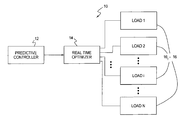
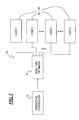
- a control system 10 includes a predictive controller 12 , a Real Time Optimizer 14 , and a plurality of loads 16 1 - 16 N .
- the loads 16 1 - 16 N can be boilers, turbines, compressors, chillers, etc.
- the predictive controller 12 suitably senses the load requirements (e.g., pressure, and/or fuel feed, and/or temperature, etc.) of the loads 16 1 - 16 N and provides a predicted total load energy demand F tot to the real time optimizer 14 that divides the total load energy demand F tot according to a predicted target allocation F i targ (k) into individual allocated fuel feed demands (or set points) F i dyn (k) for the individual loads 16 1 - 16 N .
- load requirements e.g., pressure, and/or fuel feed, and/or temperature, etc.
- the predictive controller 12 may be any of the controllers supplied by Honeywell under part numbers HT-MPC3L125, HT-MPC3L250, HT-MPC3L500, HT-MPC6L125, HT-MPC6L250, and HT-MPC6L500, or may be any other predictive controller that projects a system response to a set point, load, or other disturbance.
- the real time optimizer 14 may be any of the real time optimizers supplied by Honeywell under part numbers HT-ELA3L125, HT-ELA3L250, HT-ELA3L500, HT-ELA6L125, HT-ELA6L250, and HT-ELA6L500, or may be any other real time optimizer that can be modified so as to react to load change predictions in order to cost effectively allocate load demand among a plurality of loads.
- F tot ( F tot (1), F tot (2), . . . , F tot ( K )) (1)
- the dynamic allocation trajectories F i dyn (k) for the loads are determined by the real time optimizer 14 in two steps.
- First, the unconstrained allocation trajectories F i unconstr (k) are determined for the loads i 1, 2, . . . , N.
- the unconstrained allocation trajectories F i unconstr (k) are defined by means of two sets of parameters: (1) the target allocation F i targ (k), and (2) the dynamic weights w i dyn (k). Accordingly, the unconstrained allocation trajectories F i unconstr (k) are defined according to the following equation:
- the target allocation F i targ (k) corresponds to values around (or near) which the unconstrained allocation F i unconstr (k) varies, and the dynamic weights w i dyn (k) are an indication of the sensitivities of the loads 16 1 - 16 N to the changes in the total load demand.
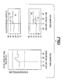
- FIG. 2 illustrates an example of dynamic fuel feed allocation with the samples on the left side of the vertical dashed line representing historical data and the samples on the right side of the vertical dashed line representing predicted (modeled) trajectories.
- the total load energy demand F tot shown in the left graph is allocated between a boiler (load) B 1 as shown in the top right graph and a boiler (load) B 2 as shown in the bottom right graph.
- the solid line curve in the graph on the left represents the total load energy demand F tot predicted by the predictive controller 12
- the horizontal dashed lines represent the target allocations F i targ (k). Moreover, for the example shown in FIG.
- the changes in total energy load demand ⁇ F tot (k) are divided into the loads 16 1 - 16 N proportionally to the dynamic weights so that the allocated load energy requirement (e.g., fuel feed value) is composed of the target value F i targ (k) plus a portion from the transient deviations ⁇ F tot (k).
- the dynamic weights may be provided by the operator. Alternatively, the dynamic weights may be calculated automatically. For example, they may be calculated automatically based on the number of running coal pulverizers, burners, etc.
- the target allocation F i targ (k) is the prediction horizon for load i and is allocated to load i by the real time optimizer 14 based upon various economic conditions.
- the target allocation F i targ (k) may be evaluated from offsets.
- the target allocation F i targ (k) is assumed to be constant during the prediction period unless the target allocation F i targ (k) is significantly changed, such as by the operator.
- the target allocation F i targ (k) is significantly changed, linear interpolation from the old value to the new one, instead of using the new value for the whole prediction period, may be used in order to assure bumpless operation.
- the target allocation F i targ (k) is set (such as by the operator as indicated above) so that it is time-invariant up to the next operator intervention, the sum of the target allocation F i targ (k) over all loads cannot follow the time-varying target of the total load energy demand F tot , i.e., the value of the total load energy demand F tot at the end of prediction horizon.
- the appreciable balance condition can be fulfilled if the target allocations F i targ (k) are evaluated using offsets F i off as given by the following equation:
- the dynamic weights w i dyn (k) may be set by the operator.
- the dynamic weights w i dyn (k) are assumed to be constant during the prediction period unless they are significantly changed by the operator. If they are changed, they may be ramped using a linear interpolation algorithm. Also, the dynamic weights w i dyn (k) are normalized to 1 as discussed above in relation to equation (6).
- the unconstrained allocation trajectories F i unconstr (k) do not need to satisfy constraints.
- the dynamic allocation trajectories F i dyn (k) are required to be constrained.
- Constraints imposed by the real time optimizer 14 may be generated by the operator. Alternatively and/or additionally, constraints may be algorithm-generated constraints that are propagated from slave controllers on all levels of a sub cascade. Also, constraints may be time varying.
- constraints may be absolute limits (such as low and high limits F i min (k) and F i min (k) on the dynamic allocation trajectories F i dyn (k)), and constraints may be rate of change limits (such as decremental and incremental limits F i ⁇ (k) and F i + (k), respectively).
- the dynamic allocation trajectories F i dyn (k) are calculated based on the unconstrained allocation trajectories F i unconstr (k).
- the dynamic allocation trajectories F i dyn (k) are constrained by the absolute constraints, considered as hard constraints, and the rate of change constraints, considered as soft constraints in that they can be violated by arbitrary (although highly penalized) values z 1 (k).
- F dyn ( F 1 dyn ⁇ F n dyn ) ( 13 )
- Expressions similar to expressions (12) can be written for F i min , F i max , F i ⁇ , F i + , and z i .
- Each of the vectors F i dyn , F i min , F i max , F i ⁇ , F i + , and Z i has a corresponding dimension K+1.
- expressions similar to expression (13) can be written for F min , F max , F ⁇ , and F + .
- Each of the vectors F dyn , F min , F max , F ⁇ , and F + has a corresponding dimension N(K+1).
- a difference vector ⁇ F i dyn is defined according to the following equation:
- D ( 1 - 1 1 - 1 1 ) ( 15 )
- the actual input energy requirements F i act may be sensed by appropriate sensors located at the energy inputs of the loads 16 1 - 16 N .
- Variables z i (k) are introduced in order to penalize violation of the rate of change constraints. If z i (k) is equal to zero (no penalty), ⁇ F i dyn (k) must lie within rate of change limits according to the inequalities (11). If ⁇ F i dyn (k) is not within corresponding limits, the variable z i (k) is equal to the deviation of ⁇ F i dyn (k) from the range ( ⁇ F i ⁇ (k),F i + (k)), and the limit violation penalty defined as the norm of z becomes non-zero.
- the dynamic demand allocation F dyn is obtained by minimizing the penalty for the deviation of F dyn from the unconstrained allocation F unconstr and for violation of the rate of change limits. That is, the dynamic allocation F dyn is obtained by minimizing the following function:
- the penalty weights w i (1) and w i (2) may be defined by the process engineer during the optimizer commissioning.
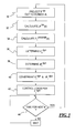
- the control algorithm as described above may be implemented by the control system 10 according to the flow chart shown in FIG. 3 .
- the total energy load demand F tot (k) is projected by the predictive controller 12 , at a block 30 of this flow chart, for each point k out to the horizon K.
- the change in F tot (k), i.e., ⁇ F tot (k) is calculated at a block 32 using equation (3) using the predicted steady state target allocations F i targ (k) set by the real time optimizer 14 as discussed above.
- the target allocations F i targ (k) may be determined in accordance with equations (7) and (8) as discussed above.
- the unconstrained allocation trajectories F i unconstr (k) are calculated at a block 34 using equation (2), where the target allocations F i targ (k) are as used at the block 32 , where the dynamic weights w i dyn (k) may be set, for example, by the operator, and where the total energy load demand F tot (k) is provided by the block 30 .
- the dynamic demand allocation trajectories F i dyn (k) are then determined at a block 36 in accordance with equations (17), (18), and (19), and the difference vector ⁇ F i dyn is determined at a block 38 in accordance with equations (14), (15), and (16). Constraints are applied to the dynamic allocation trajectories F i dyn (k) and the difference vector ⁇ F i dyn at a block 40 in accordance with equations (9), (10), and (11).
- the constrained dynamic demand allocation trajectories F i dyn (k) are used to control energy supplied to the respective loads 1 , . . . , N.
- the algorithm at a block 44 then waits for the next time k before repeating the operations of the blocks ( 30 )-( 44 ).
- the target allocation F i targ (k) is provided by a Real Time Optimizer.
- the target allocation F i targ (k) may be set by an operator.
Abstract
Loads 1, 2, . . . , N are controlled by predicting a total energy requirement for the loads 1, 2, . . . , N at prediction points k=0, 1, 2, . . . , K, by allocating the total energy requirement to the loads 1, 2, . . . , N at prediction points k=0, 1, 2, . . . , K, by determining a dynamic energy demand requirement for each of the loads 1, 2, . . . , N at prediction points k=0, 1, 2, . . . , K based on the allocated energy requirements, and by controlling the loads 1, 2, . . . , N based on the dynamic energy demand requirements.
Description
The present invention relates to dynamic load control.
Controls have been developed for a variety of different load control processes. For example, in steam generation plants, several boilers and/or other types of steam generators generate steam and supply the steam to a common header. If individual pressure controllers with integral action running in parallel were used to control the boilers, instability in the operation of the boilers could result.
Therefore, pressure in the header is typically controlled by a single master pressure controller (MPC) that produces a total energy requirement (usually in terms of fuel feed) for the plant input. An energy allocation module divides the total energy requirement into separate fuel feed demands (i.e., set points) for the individual boilers.
The division of the total energy requirement implemented by the energy allocation module should be cost optimized according to varying economic conditions (such as price of fuels and electricity, environmental limits, etc.) and according to various constraints such as total production demand, technological constraints, runtime hours, and life time consumption. The underlying optimization problem is well known and has been solved in a variety of ways and with various levels of complexity since the 1960's. For example, Real Time Optimizers have been implemented in order to optimize the cost of operating one or more loads.
These Real Time Optimizers have detected a steady state load requirement and then have provided control signals that optimize the cost of operating the loads based on this steady state load requirement. In order to operate in this fashion, the Real Time Optimizers have had to wait for transient process disturbances to settle out so that a steady state condition exists before such Optimizers can invoke their optimization procedures. However, for processes with slow dynamics and/or high levels of disturbances, the dependence of Real Time Optimizers on steady state information substantially deteriorates the performance of the control system, as no optimization is performed during the transients created by disturbances such as changes in set point and/or changes in load.
While predictive controllers have been used in the past, predictive controllers have not been used with Real Time Optimizers such that the Real Time Optimizers dynamically respond to target load values of the predicted process variables projected to the end of a prediction horizon. In one embodiment of the present invention, predictive controllers and Real Time Optimization are combined in this fashion in order to more effectively control loads during disturbances such as changes in set point and changes in load.
According to one aspect of the present invention, a process control system for controlling a load comprises a predictive controller and a real time optimizer. The predictive controller predicts an energy requirement for the load at prediction points k=0, 1, 2, . . . , K based on a steady state target energy requirement for the load. The real time optimizer determines an optimized dynamic energy demand requirement for the load at the prediction points k=0, 1, 2, . . . , K based on the predicted energy requirement, and controls the load based on the dynamic energy demand requirement.
According to another aspect of the present invention, a process control method for controlling loads 1, 2, . . . , N comprises the following: predicting, in a predictive controller, an energy requirement for each of the loads 1, 2, . . . , N at prediction points k=0, 1, 2, . . . , K based on a steady state target allocation for each of the loads 1, 2, . . . , N; determining, in a real time optimizer, a dynamic energy demand requirement for each of the loads 1, 2, . . . , N at prediction points k=0, 1, 2, . . . , K based on the predicted energy requirements; and, controlling the loads 1, 2, . . . , N based on the dynamic energy demand requirements.
According to yet another aspect of the present invention, a process control method for controlling loads 1, 2, . . . , N comprises the following: predicting, by way of a predictive controller, a total energy requirement for the loads 1, 2, . . . , N at prediction points k=0, 1, 2, . . . , K; allocating, by way of a real time optimizer, the total energy requirement to the loads 1, 2, . . . , N at the prediction points k=0, 1, 2, . . . , K based on a steady state target for each of the loads 1, 2, . . . , N; determining, by way of the real time optimizer, a dynamic energy demand requirement for each of the loads 1, 2, . . . , N at the prediction points k=0, 1, 2, . . . , K based on the allocated energy requirements; and, controlling the loads 1, 2, . . . , N based on the dynamic energy demand requirements.
These and other features and advantages will become more apparent from a detailed consideration of the invention when taken in conjunction with the drawings in which:
FIG. 1 illustrates a control system according to an embodiment of the invention;
FIG. 2 illustrate graphs useful in explaining the present invention; and,
FIG. 3 illustrates a flow chart depicting the operation of the control system shown in FIG. 1.
In one embodiment of the present invention, real-time, on-line, optimized dynamic allocation of time varying total demand among loads, taking into account various constraints, is provided. The resulting dynamic allocation is composed of a target allocation Fi targ(k) and a dynamic portion wi dyn(k)ΔFtot(k) that is proportional to the loads' dynamic weights wi dyn(k) for loads i=1, . . . , N. The target allocation Fi targ(k) is provided by a Real Time Optimizer using load cost curves which can be evaluated from efficiency or consumption curves, etc. Likewise, the loads' dynamic weights wi dyn(k) may also be set by the Real Time Optimizer or by an operator.
The algorithm that implements the optimized dynamic allocation is used with a model-based predictive controller. In this case, a steady state load balance at the end of a prediction horizon can be predicted as the target value for computation of the target economic allocation, and dynamic deviations in the transient part of the prediction period can be allocated in proportion to the dynamic weights. In this way, the system of the present invention need not wait for loads to achieve a steady state condition following a disturbance to economically control the loads.
Moreover, because a predictive controller is used, rate of change constraints, in addition to the absolute constraints, are introduced so as to provide a positive impact on the stability of the control process and on the stresses and life time of the control system equipment.
The algorithm that is implemented by the control system may be modular. For example, the target allocation Fi targ(k) is provided by an optimization routine using the loads' cost curves which can be evaluated from efficiency curves, etc. This modular structure allows the addition of new features that, for example, take into account burner configuration, fuel mixing, etc. without changing the basic algorithm. An off-line what-if analysis as a decision support tool is also possible using existing routines.
As shown in FIG. 1, a control system 10 includes a predictive controller 12, a Real Time Optimizer 14, and a plurality of loads 16 1-16 N. For example, the loads 16 1-16 N can be boilers, turbines, compressors, chillers, etc. Thus, if i=1, 2, . . . , N designates the loads 16 1-16 N in FIG. 1, then N designates the number of loads.
The predictive controller 12 suitably senses the load requirements (e.g., pressure, and/or fuel feed, and/or temperature, etc.) of the loads 16 1-16 N and provides a predicted total load energy demand Ftot to the real time optimizer 14 that divides the total load energy demand Ftot according to a predicted target allocation Fi targ(k) into individual allocated fuel feed demands (or set points) Fi dyn(k) for the individual loads 16 1-16 N.
The predictive controller 12 may be any of the controllers supplied by Honeywell under part numbers HT-MPC3L125, HT-MPC3L250, HT-MPC3L500, HT-MPC6L125, HT-MPC6L250, and HT-MPC6L500, or may be any other predictive controller that projects a system response to a set point, load, or other disturbance. The real time optimizer 14 may be any of the real time optimizers supplied by Honeywell under part numbers HT-ELA3L125, HT-ELA3L250, HT-ELA3L500, HT-ELA6L125, HT-ELA6L250, and HT-ELA6L500, or may be any other real time optimizer that can be modified so as to react to load change predictions in order to cost effectively allocate load demand among a plurality of loads.
Because the predictive controller 12 is a predictive controller, the total load energy demand Ftot is a trajectory, i.e., a sequence of values corresponding to a sequence of prediction times k up to a prediction horizon K, where k=0, 1, . . . , K. Accordingly, the total load energy demand Ftot may be given by the following equation:
The dynamic allocation trajectories Fi dyn(k) for the loads are determined by the real time optimizer 14 in two steps. First, the unconstrained allocation trajectories Fi unconstr(k) are determined for the loads i=1, 2, . . . , N. Second, the unconstrained allocation trajectories Fi unconstr(k) for the loads i=1, 2, . . . , N are modified to satisfy constraints and to approach the unconstrained allocation as much as possible (in the sense of minimum least squares of deviations) in order to obtain the dynamic allocation trajectories Fi dyn(k).
In the first step, the unconstrained allocation trajectories Fi unconstr(k) are defined by means of two sets of parameters: (1) the target allocation Fi targ(k), and (2) the dynamic weights wi dyn(k). Accordingly, the unconstrained allocation trajectories Fi unconstr(k) are defined according to the following equation:
where 
for each load i=1, 2, . . . , N and for each trajectory point k=0, 1, . . . , K.
The target allocation Fi targ(k) corresponds to values around (or near) which the unconstrained allocation Fi unconstr(k) varies, and the dynamic weights wi dyn(k) are an indication of the sensitivities of the loads 16 1-16 N to the changes in the total load demand.
FIG. 2 illustrates an example of dynamic fuel feed allocation with the samples on the left side of the vertical dashed line representing historical data and the samples on the right side of the vertical dashed line representing predicted (modeled) trajectories. The samples may be taken at time instants tk=kTs, where Ts is a given sampling period. The total load energy demand Ftot shown in the left graph is allocated between a boiler (load) B1 as shown in the top right graph and a boiler (load) B2 as shown in the bottom right graph. The dashed curves 20 and 22 represent the unconstrained allocation trajectories Fi=1 unconstr(k) and Fi=2 unconstr(k) for loads B1 and B2, respectively. The solid line curve in the graph on the left represents the total load energy demand Ftot predicted by the predictive controller 12, and the solid line curves in the graphs on the right represent the dynamically allocation fuel feeds (set points) Fi=1 dyn(k) and Fi=2 dyn(k) for loads B1 and B2, respectively, as produced by the real time optimizer 14. The horizontal solid lines represent absolute limits that are placed on the total load energy demand Ftot and the dynamically allocation fuel feeds (set points) Fi=1 dyn(k) and Fi=2 dyn(k), respectively. The horizontal dashed lines represent the target allocations Fi targ(k). Moreover, for the example shown in FIG. 2, the ratio of the dynamic weights used for loads B1 and B2 are assumed to be given by the following equation: 
Accordingly, the changes in total energy load demand ΔFtot(k) are divided into the loads 16 1-16 N proportionally to the dynamic weights so that the allocated load energy requirement (e.g., fuel feed value) is composed of the target value Fi targ(k) plus a portion from the transient deviations ΔFtot(k). The dynamic weights may be provided by the operator. Alternatively, the dynamic weights may be calculated automatically. For example, they may be calculated automatically based on the number of running coal pulverizers, burners, etc.
A balance condition exists where the sum over the loads 16 1-16 N of the target allocations 
is equal to total load energy demand Ftot(k) in equation (3). In the balance condition, ΔFtot(k) is zero, and the following relationship: 
is fulfilled for each trajectory point k, assuming that the non-negative dynamic weights are normalized to 1 according to the following equation: 
As discussed above, the target allocation Fi targ(k) is the prediction horizon for load i and is allocated to load i by the real time optimizer 14 based upon various economic conditions. The target allocation Fi targ(k) may be evaluated from offsets.
As indicated by FIG. 2, the target allocation Fi targ(k) is assumed to be constant during the prediction period unless the target allocation Fi targ(k) is significantly changed, such as by the operator. When the target allocation Fi targ(k) is significantly changed, linear interpolation from the old value to the new one, instead of using the new value for the whole prediction period, may be used in order to assure bumpless operation.
If the target allocation Fi targ(k) is set (such as by the operator as indicated above) so that it is time-invariant up to the next operator intervention, the sum of the target allocation Fi targ(k) over all loads cannot follow the time-varying target of the total load energy demand Ftot, i.e., the value of the total load energy demand Ftot at the end of prediction horizon. However, the appreciable balance condition can be fulfilled if the target allocations Fi targ(k) are evaluated using offsets Fi off as given by the following equation:
where Fav is determined from the following balance condition: 
Thus, even if offsets (defining differences between loads) are constant, the term 
is time varying and equal to Ftot(K).
As indicated above, the dynamic weights wi dyn(k) may be set by the operator. The dynamic weights wi dyn(k) are assumed to be constant during the prediction period unless they are significantly changed by the operator. If they are changed, they may be ramped using a linear interpolation algorithm. Also, the dynamic weights wi dyn(k) are normalized to 1 as discussed above in relation to equation (6).
As indicated above, the unconstrained allocation trajectories Fi unconstr(k) do not need to satisfy constraints. On the other hand, the dynamic allocation trajectories Fi dyn(k) are required to be constrained. Constraints imposed by the real time optimizer 14 may be generated by the operator. Alternatively and/or additionally, constraints may be algorithm-generated constraints that are propagated from slave controllers on all levels of a sub cascade. Also, constraints may be time varying. Moreover, constraints may be absolute limits (such as low and high limits Fi min(k) and Fi min(k) on the dynamic allocation trajectories Fi dyn(k)), and constraints may be rate of change limits (such as decremental and incremental limits Fi −(k) and Fi +(k), respectively).
While absolute constraints must not be violated, rate of change constraints can be violated. However, such a violation should be highly penalized so as to avoid undesired thermal stress, which may have a negative impact on the life of the control system equipment.
In the second step of calculating the dynamic allocation trajectories Fi dyn(k), the dynamic allocation trajectories Fi dyn(k) are calculated based on the unconstrained allocation trajectories Fi unconstr(k). The dynamic allocation trajectories Fi dyn(k) must satisfy the total load energy demand Ftot (as the unconstrained allocation trajectories Fi unconstr(k) must also do) according to the following equation: 
In addition, the dynamic allocation trajectories Fi dyn(k) are constrained by the absolute constraints, considered as hard constraints, and the rate of change constraints, considered as soft constraints in that they can be violated by arbitrary (although highly penalized) values z1(k).
These constraints are given by the following expressions:
where 
Expressions similar to expressions (12) can be written for Fi min, Fi max, Fi −, Fi +, and zi. Each of the vectors Fi dyn, Fi min, Fi max, Fi −, Fi +, and Zi has a corresponding dimension K+1. Also, expressions similar to expression (13) can be written for Fmin, Fmax, F−, and F+. Each of the vectors Fdyn, Fmin, Fmax, F−, and F+ has a corresponding dimension N(K+1).
A difference vector ΔFi dyn is defined according to the following equation:
where D is a (K+1) by (K+1) difference matrix given by the following equation: 
and where Fi act are (K+1) dimensional vectors having the corresponding loads' actual input energy requirements (such as boilers' actual fuel feed) in the first component and zeros elsewhere as given by the following equation: 
The actual input energy requirements Fi act may be sensed by appropriate sensors located at the energy inputs of the loads 16 1-16 N.
Variables zi(k) are introduced in order to penalize violation of the rate of change constraints. If zi(k) is equal to zero (no penalty), ΔFi dyn(k) must lie within rate of change limits according to the inequalities (11). If ΔFi dyn(k) is not within corresponding limits, the variable zi(k) is equal to the deviation of ΔFi dyn(k) from the range (−Fi −(k),Fi +(k)), and the limit violation penalty defined as the norm of z becomes non-zero.
The dynamic demand allocation Fdyn is obtained by minimizing the penalty for the deviation of Fdyn from the unconstrained allocation Funconstr and for violation of the rate of change limits. That is, the dynamic allocation Fdyn is obtained by minimizing the following function:
with respect to variables Fdyn and z, subject to constraints (9)-(11). It should be noted that the vector Funconstr in equation (17) has a dimension 2N(K+1) similar to the right hand side of equation (13). Function (17) is a quadratic programming problem with dimension 2N(K+1)
The square N(K+1) by N(K+1) norm matrices Q(1) and Q(2) can be chosen as diagonal matrices with elements depending only on boiler i, not on trajectory points k. Accordingly, these matrices may be given by the following equations: 
q i (j) =w i (j) I (19)
where j=1, 2, where I is a (K+1) by (K+1) unity matrix, and where wi (1) and wi (2) are penalty weights for i=1, . . . N. The penalty weights wi (1) and wi (2) may be defined by the process engineer during the optimizer commissioning.
The control algorithm as described above may be implemented by the control system 10 according to the flow chart shown in FIG. 3. With k equal to a current value, the total energy load demand Ftot(k) is projected by the predictive controller 12, at a block 30 of this flow chart, for each point k out to the horizon K. The change in Ftot(k), i.e., ΔFtot(k), is calculated at a block 32 using equation (3) using the predicted steady state target allocations Fi targ(k) set by the real time optimizer 14 as discussed above. Alternatively, the target allocations Fi targ(k) may be determined in accordance with equations (7) and (8) as discussed above. Also, the unconstrained allocation trajectories Fi unconstr(k) are calculated at a block 34 using equation (2), where the target allocations Fi targ(k) are as used at the block 32, where the dynamic weights wi dyn(k) may be set, for example, by the operator, and where the total energy load demand Ftot(k) is provided by the block 30.
The dynamic demand allocation trajectories Fi dyn(k) are then determined at a block 36 in accordance with equations (17), (18), and (19), and the difference vector ΔFi dyn is determined at a block 38 in accordance with equations (14), (15), and (16). Constraints are applied to the dynamic allocation trajectories Fi dyn(k) and the difference vector ΔFi dyn at a block 40 in accordance with equations (9), (10), and (11). At a block 42, the constrained dynamic demand allocation trajectories Fi dyn(k) are used to control energy supplied to the respective loads 1, . . . , N.
The algorithm at a block 44 then waits for the next time k before repeating the operations of the blocks (30)-(44).
Certain modifications of the present invention has been described above. Other modifications of the invention will occur to those skilled in the art. For example, although the present invention has been described above with specific reference to the control of loads such as boilers, the present invention may be used in connection with a variety of other control processes.
Also as described above, the target allocation Fi targ(k) is provided by a Real Time Optimizer. Alternatively, the target allocation Fi targ(k) may be set by an operator.
Accordingly, the description of the present invention is to be construed as illustrative only and is for the purpose of teaching those skilled in the art the best mode of carrying out the invention. The details may be varied substantially without departing from the spirit of the invention, and the exclusive use of all modifications which are within the scope of the appended claims is reserved.
Claims (51)
1. A process control system for controlling a load comprising:
a predictive controller that predicts an energy requirement for the load at prediction points k =0, 1, 2, . . , K based on a steady state target energy requirement for the load; and,
a real time cost optimizer that determines a cost optimized dynamic energy demand requirement for the load at the prediction points k =0, 1, 2, . . . , K based on the predicted energy requirement and that controls the load based on the dynamic energy demand requirement.
2. The process control system of claim 1 wherein the real time optimizer is arranged to constrain the dynamic energy demand requirement to a limit and controls the load based on the constrained dynamic energy demand requirement.
3. The process control system of claim 2 wherein the limit comprises a maximum limit.
4. The process control system of claim 2 wherein the limit comprises a minimum limit.
5. The process control system of claim 2 wherein the limit comprises a minimum limit and a maximum limit.
6. The process control system of claim 2 wherein the real time optimizer determines ΔFdyn according to the following equation:
wherein D is a (K+1) by (K+1) matrix given by the following equation: 
and wherein Fact is a (K+1) dimensional vector representing an actual energy consumption of the load in the first component and zeros elsewhere as given by the following equation: 
wherein Fdyn is the dynamic energy demand requirement, and wherein ΔFdyn is constrained to a limit.
7. The process control system of claim 6 wherein the limit for ΔFdyn comprises a maximum limit.
8. The process control system of claim 6 wherein the limit for ΔFdyn comprises a minimum limit.
9. The process control system of claim 6 wherein the limit for ΔFdyn comprises a minimum limit and a maximum limit.
10. The process control system of claim 1 wherein the predicted energy requirement is designated Funconstr, wherein the dynamic energy demand requirement is designated Fdyn, and wherein Fdyn is determined by minimizing a quadratic function based on a difference between Funconstr and Fdyn.
11. The process control system of claim 10 wherein Funconstr and Fdyn each have dimensions K+1.
12. The process control system of claim 10 wherein the real time controller is arranged to constrain Fdyn to a limit and to control the load based on the constrained Fdyn.
13. The process control system of claim 12 wherein the limit comprises a maximum limit.
14. The process control system of claim 12 wherein the limit comprises a minimum limit.
15. The process control system of claim 12 wherein the limit comprises a minimum limit and a maximum limit.
16. A process control method for controlling parallel loads 1, 2, . . . , N comprising:
predicting, in a predictive controller, an energy requirement for each of the loads 1, 2, . . . , N at prediction points k=0, 1, 2, . . . , K based on a steady state target allocation for each of the parallel loads 1, 2, . . . , N;
determining, in a real time optimizer, a dynamic energy demand requirement for each of the parallel loads 1, 2, . . . , N at prediction points k=0, 1, 2, . . . , K based on the predicted energy requirements so as to cost effectively allocate load demand among the parallel load 1, 2, . . . , N; and,
controlling the loads 1, 2, . . . , N based on the dynamic energy demand requirements.
17. The process control method of claim 16 wherein the controlling of the loads based on the dynamic energy demand requirements comprises:
constraining each of the dynamic energy demand requirements to a corresponding limit; and,
controlling the loads 1, 2, . . . , N based on the corresponding constrained dynamic energy demand requirements.
18. The process control method of claim 17 wherein the corresponding limits comprise corresponding maximum limits.
19. The process control method of claim 17 wherein the corresponding limits comprise corresponding minimum limits.
20. The process control method of claim 17 wherein the corresponding limits comprise corresponding minimum limits and corresponding maximum limits.
21. The process control method of claim 17 further comprising;
determining ΔFi dyn according to the following equation:
wherein D is a (K+1) by (K+1) matrix given by the following equation: 
and wherein Fi act is a (K+1) dimensional vector having an actual energy consumption of a corresponding one of the loads in the first component and zeros elsewhere as given by the following equation: 
wherein i=1, 2, . . . , N designates the loads, wherein Fi dyn designate the dynamic energy demand requirements of the loads 1, 2, . . . , N, and wherein ΔFi dyn are constrained to corresponding limits.
22. The process control method of claim 21 wherein the corresponding limits for ΔFi dyn comprise corresponding maximum limits.
23. The process control method of claim 21 wherein the corresponding limits for ΔFi dyn comprise corresponding minimum limits.
24. The process control method of claim 21 wherein the corresponding limits for ΔFi dyn comprise corresponding minimum limits and corresponding maximum limits.
25. The process control method of claim 16 wherein the predicted energy requirement for each of the loads 1, 2, . . . , N is designated Fi unconstr, wherein the dynamic energy demand requirement for each of the loads 1, 2, . . . , N is designated Fi dyn, wherein Fi dyn is determined by minimizing the following quadratic function:
with respect to variables Fdyn and z, wherein Fdyn and Funconstr are vectors each having a dimension 2N(K+1), wherein Q(1) and Q(2) are each square N(K+1) by N(K+1) norm matrices given by the following equations: 
q i (j) =w i (j) I
wherein I is a (K+1) by (K+1) unity matrix, wherein wi (1) and wi (2) are penalty weights for i=1, . . . , N, and wherein z is a penalty vector having a 2N(K+1) dimension.
26. The process control method of claim 25 wherein Funconstr and Fdyn each have dimensions K+1.
27. The process control method of claim 25 wherein the controlling of the loads 1, 2, . . . , N based on the dynamic energy demand requirements comprises:
constraining Fi dyn to corresponding limits; and,
controlling the load based on the constrained FI dyn.
28. The process control method of claim 27 wherein the corresponding limits comprise corresponding maximum limits.
29. The process control method of claim 27 wherein the corresponding limits comprise corresponding minimum limits.
30. The process control method of claim 27 wherein the corresponding limits comprise corresponding minimum limits and maximum limits.
31. A process control method for controlling parallel loads 1, 2, . . . , N comprising:
predicting, by way of a predictive controller, a total energy requirement for the parallel loads 1, 2, . . . , N at prediction points k=0, 1, 2, . . . , K;
allocating, on a cost effective basis by way of a real time optimizer, the total energy requirement to the parallel loads 1, 2, . . . , N at the prediction points k=0, 1, 2, . . . , K based on a steady state target for each of the parallel loads 1, 2, . . . , N;
determining, by way of the real time optimizer, a dynamic energy demand requirement for each of the parallel loads 1, 2, . . . , N at the prediction points k=0, 1, 2, . . . , K based on the allocated energy requirements; and,
controlling the parallel loads 1, 2, . . . , N based on the dynamic energy demand requirements.
32. The process control method of claim 31 wherein the allocating of the total energy requirement to the loads 1, 2, . . . , N comprises:
determining a change ΔFtot(k) in the total energy requirement according to the following equation: 
for each of the parallel loads i=1, 2, . . . , N and for each of the prediction points k=0, 1, . . . , K; and,
allocating the total energy requirement to the loads 1, 2, . . . , N at prediction points k=0, 1, 2, . . . , K according to the following equation:
wherein Fi targ(k) are the steady state targets for the loads 1, 2, . . . , N, and wherein wi dyn(k) are weights determining the allocation of the total energy requirement.
33. The process control method of claim 32 wherein wi dyn(k) are set by an operator.
34. The process control method of claim 32 wherein wi dyn(k) are set by an economic load allocation module.
35. The process control method of claim 32 wherein Fi targ(k) are set by an operator.
36. The process control method of claim 32 wherein Fi targ(k) are set by an economic load allocation module.
37. The process control method of claim 31 wherein the controlling of the loads 1, 2, . . . , N based on the dynamic energy demand requirements comprises:
constraining each of the dynamic energy demand requirements to a corresponding limit; and,
controlling the loads 1, 2, . . . , N based on the corresponding constrained dynamic energy demand requirements.
38. The process control method of claim 37 wherein the corresponding limits comprise corresponding maximum limits.
39. The process control method of claim 37 wherein the corresponding limits comprise corresponding minimum limits.
40. The process control method of claim 37 wherein the corresponding limits comprise corresponding minimum limits and corresponding maximum limits.
41. The process control method of claim 31 wherein the total energy requirements allocated to the loads 1, 2, . . . , N at prediction points k=0, 1, 2, . . . , K are designated Fi dyn, and wherein the process control method further comprises;
determining a change ΔFi dyn in the total energy requirements allocated to the loads 1, 2, . . . , N according to the following equation:
wherein D is a (K+1) by (K+1) matrix given by the following equation: 
and wherein Fi act is a (K+1) dimensional vector having an actual energy consumption of the corresponding loads in the first component and zeros elsewhere as given by the following equation: 
wherein i=1, 2, . . . , N designates the loads, and wherein ΔFi dyn is constrained to a corresponding limit.
42. The process control method of claim 41 wherein the corresponding limits for ΔFi dyn comprise corresponding maximum limits.
43. The process control method of claim 41 wherein the corresponding limits for ΔFi dyn comprise corresponding minimum limits.
44. The process control method of claim 41 wherein the corresponding limits for ΔFi dyn comprise corresponding minimum limits and corresponding maximum limits.
45. The process control method of claim 31 wherein the total energy requirement allocated to each of the loads 1, 2, . . . , N is designated Fi unconstr, wherein the dynamic energy demand requirement for each of the loads 1, 2, . . . , N is designated Fi dyn, and wherein Fi dyn is determined by minimizing the following quadratic function:
with respect to variables Fdyn and z, wherein Fdyn and Funconstr are vectors each having a dimension 2N(K+1), wherein Q(1) and Q(2) are each square N(K+1) by N(K+1) norm matrices given by the following equations: 
q i (j) =w i (j) I
wherein j =1, 2, wherein I is a (K+1) by (K+1) unity matrix, wherein wi (1) and wi (2) are penalty weights for i=1, . . . , N, and wherein z is a penalty vector having a 2N(K+1) dimension.
46. The process control method of claim 45 wherein Funconstr and Fdyn each have dimensions K+1.
47. The process control method of claim 45 wherein the controlling of the loads 1, 2, . . . , N based on the dynamic energy demand requirements comprises:
constraining Fi dyn to corresponding limits; and,
controlling the load based on the constrained Fi dyn.
48. The process control method of claim 47 wherein the corresponding limits comprise corresponding maximum limits.
49. The process control method of claim 47 wherein the corresponding limits comprise corresponding minimum limits.
50. The process control method of claim 47 wherein the corresponding limits comprise corresponding minimum limits and maximum limits.
51. A process control system for controlling loads comprising:
a predictive controller that predicts energy requirements for the loads by projecting the energy requirements out to the end of a prediction horizon; and,
a real time cost optimizer that dynamically responds to the predicted energy requirements by dynamically determining cost optimized dynamic energy demand requirements for the loads and by controlling the loads based on the dynamically determined energy demand requirements.
Priority Applications (6)
| Application Number | Priority Date | Filing Date | Title |
|---|---|---|---|
| US10/292,708 US6832134B2 (en) | 2002-11-12 | 2002-11-12 | Coordination in multilayer process control and optimization schemes |
| PCT/US2003/035569 WO2004044663A1 (en) | 2002-11-12 | 2003-11-07 | Coordination in multilayer process control and optimization schemes |
| DE60329521T DE60329521D1 (en) | 2002-11-12 | 2003-11-07 | COORDINATION OF MULTILAYER PROCESS CONTROL AND OPTIMIZATION PROCESS |
| CN200380108343.XA CN1735846A (en) | 2002-11-12 | 2003-11-07 | Coordination in multilayer process control and optimization schemes |
| EP03781818A EP1563347B1 (en) | 2002-11-12 | 2003-11-07 | Coordination in multilayer process control and optimization schemes |
| AU2003287573A AU2003287573A1 (en) | 2002-11-12 | 2003-11-07 | Coordination in multilayer process control and optimization schemes |
Applications Claiming Priority (1)
| Application Number | Priority Date | Filing Date | Title |
|---|---|---|---|
| US10/292,708 US6832134B2 (en) | 2002-11-12 | 2002-11-12 | Coordination in multilayer process control and optimization schemes |
Publications (2)
| Publication Number | Publication Date |
|---|---|
| US20040093124A1 US20040093124A1 (en) | 2004-05-13 |
| US6832134B2 true US6832134B2 (en) | 2004-12-14 |
Family
ID=32229510
Family Applications (1)
| Application Number | Title | Priority Date | Filing Date |
|---|---|---|---|
| US10/292,708 Expired - Lifetime US6832134B2 (en) | 2002-11-12 | 2002-11-12 | Coordination in multilayer process control and optimization schemes |
Country Status (6)
| Country | Link |
|---|---|
| US (1) | US6832134B2 (en) |
| EP (1) | EP1563347B1 (en) |
| CN (1) | CN1735846A (en) |
| AU (1) | AU2003287573A1 (en) |
| DE (1) | DE60329521D1 (en) |
| WO (1) | WO2004044663A1 (en) |
Cited By (8)
| Publication number | Priority date | Publication date | Assignee | Title |
|---|---|---|---|---|
| US20040257858A1 (en) * | 2003-05-13 | 2004-12-23 | Ashmin Mansingh | Dynamic economic dispatch for the management of a power distribution system |
| US20050228545A1 (en) * | 2002-03-28 | 2005-10-13 | Toshihiko Tanaka | Electric power plant general control system |
| US20060085098A1 (en) * | 2004-10-20 | 2006-04-20 | Childress Ronald L Jr | Predictive header pressure control |
| US20130297089A1 (en) * | 2011-09-12 | 2013-11-07 | Sheau-Wei J. Fu | Power management control system |
| US20150018985A1 (en) * | 2013-07-11 | 2015-01-15 | Honeywell International Inc. | Predicting responses of resources to demand response signals and having comfortable demand responses |
| US10324429B2 (en) | 2014-03-25 | 2019-06-18 | Honeywell International Inc. | System for propagating messages for purposes of demand response |
| US10541556B2 (en) | 2017-04-27 | 2020-01-21 | Honeywell International Inc. | System and approach to integrate and manage diverse demand response specifications for multi-site enterprises |
| US10762454B2 (en) | 2009-07-17 | 2020-09-01 | Honeywell International Inc. | Demand response management system |
Families Citing this family (25)
| Publication number | Priority date | Publication date | Assignee | Title |
|---|---|---|---|---|
| US7209838B1 (en) * | 2003-09-29 | 2007-04-24 | Rockwell Automation Technologies, Inc. | System and method for energy monitoring and management using a backplane |
| US7373222B1 (en) | 2003-09-29 | 2008-05-13 | Rockwell Automation Technologies, Inc. | Decentralized energy demand management |
| US7310572B2 (en) * | 2005-09-16 | 2007-12-18 | Honeywell International Inc. | Predictive contract system and method |
| US20070088448A1 (en) * | 2005-10-19 | 2007-04-19 | Honeywell International Inc. | Predictive correlation model system |
| JP5114026B2 (en) * | 2006-06-28 | 2013-01-09 | 三洋電機株式会社 | Demand control device |
| US8321800B2 (en) | 2007-07-26 | 2012-11-27 | Areva T & D, Inc. | Methods for creating dynamic lists from selected areas of a power system of a utility company |
| US8069359B2 (en) * | 2007-12-28 | 2011-11-29 | Intel Corporation | System and method to establish and dynamically control energy consumption in large-scale datacenters or IT infrastructures |
| US7937928B2 (en) * | 2008-02-29 | 2011-05-10 | General Electric Company | Systems and methods for channeling steam into turbines |
| US9760067B2 (en) | 2009-09-10 | 2017-09-12 | Honeywell International Inc. | System and method for predicting future disturbances in model predictive control applications |
| JP5510019B2 (en) * | 2010-04-16 | 2014-06-04 | 富士通株式会社 | Power control method, program and apparatus |
| US9558250B2 (en) * | 2010-07-02 | 2017-01-31 | Alstom Technology Ltd. | System tools for evaluating operational and financial performance from dispatchers using after the fact analysis |
| US9093840B2 (en) * | 2010-07-02 | 2015-07-28 | Alstom Technology Ltd. | System tools for integrating individual load forecasts into a composite load forecast to present a comprehensive synchronized and harmonized load forecast |
| US8538593B2 (en) | 2010-07-02 | 2013-09-17 | Alstom Grid Inc. | Method for integrating individual load forecasts into a composite load forecast to present a comprehensive synchronized and harmonized load forecast |
| US20110029142A1 (en) * | 2010-07-02 | 2011-02-03 | David Sun | System tools that provides dispatchers in power grid control centers with a capability to make changes |
| US20110071690A1 (en) * | 2010-07-02 | 2011-03-24 | David Sun | Methods that provide dispatchers in power grid control centers with a capability to manage changes |
| US9727828B2 (en) * | 2010-07-02 | 2017-08-08 | Alstom Technology Ltd. | Method for evaluating operational and financial performance for dispatchers using after the fact analysis |
| US8972070B2 (en) | 2010-07-02 | 2015-03-03 | Alstom Grid Inc. | Multi-interval dispatch system tools for enabling dispatchers in power grid control centers to manage changes |
| ES2395659B1 (en) * | 2011-06-30 | 2013-05-23 | Universidad Nacional De Educación A Distancia | METHOD AND GUIDANCE SYSTEM BY DERIVATIVE CONTROL. |
| US9163828B2 (en) * | 2011-10-31 | 2015-10-20 | Emerson Process Management Power & Water Solutions, Inc. | Model-based load demand control |
| CN103617548B (en) * | 2013-12-06 | 2016-11-23 | 中储南京智慧物流科技有限公司 | A kind of medium-term and long-term needing forecasting method of tendency, periodically commodity |
| NL2021038B1 (en) * | 2018-06-01 | 2019-12-10 | Stork Thermeq B V | Steam boiler assembly |
| JP7107073B2 (en) * | 2018-08-02 | 2022-07-27 | 三浦工業株式会社 | By-product gas utilization system |
| CN109870924B (en) * | 2019-01-18 | 2021-06-01 | 昆明理工大学 | Distributed system control method for model predictive control by applying multilayer steady-state target calculation |
| CN110794679A (en) * | 2019-11-08 | 2020-02-14 | 浙江大学 | Prediction control method and system for load regulation of industrial steam supply system |
| CN111290283B (en) * | 2020-04-03 | 2021-07-27 | 福州大学 | Additive manufacturing single machine scheduling method for selective laser melting process |
Citations (13)
| Publication number | Priority date | Publication date | Assignee | Title |
|---|---|---|---|---|
| US4110825A (en) * | 1977-04-28 | 1978-08-29 | Westinghouse Electric Corp. | Control method for optimizing the power demand of an industrial plant |
| US4532761A (en) | 1982-09-10 | 1985-08-06 | Tokyo Shibaura Denki Kabushiki Kaisha | Load control system and method of combined cycle turbine plants |
| GB2166198A (en) | 1984-10-25 | 1986-04-30 | Westinghouse Electric Corp | Improved steam turbine load control in a combined cycle electrical power plant |
| EP0465137A1 (en) | 1990-06-28 | 1992-01-08 | General Electric Company | Control of a combined cycle turbine |
| US5268835A (en) * | 1990-09-19 | 1993-12-07 | Hitachi, Ltd. | Process controller for controlling a process to a target state |
| US5704011A (en) * | 1994-11-01 | 1997-12-30 | The Foxboro Company | Method and apparatus for providing multivariable nonlinear control |
| US6438430B1 (en) * | 1996-05-06 | 2002-08-20 | Pavilion Technologies, Inc. | Kiln thermal and combustion control |
| US6439469B1 (en) | 1999-08-02 | 2002-08-27 | Siemens Building Technologies Ag | Predictive apparatus for regulating or controlling supply values |
| US20030018399A1 (en) * | 1996-05-06 | 2003-01-23 | Havener John P. | Method for optimizing a plant with multiple inputs |
| US6591225B1 (en) * | 2000-06-30 | 2003-07-08 | General Electric Company | System for evaluating performance of a combined-cycle power plant |
| US6597958B1 (en) * | 2001-03-22 | 2003-07-22 | Abb Automation Inc. | Method for measuring the control performance provided by an industrial process control system |
| US6681155B1 (en) * | 1998-08-31 | 2004-01-20 | Mitsubishi Chemical Corporation | Optimizing control method and optimizing control system for power plant |
| US6714899B2 (en) * | 1998-09-28 | 2004-03-30 | Aspen Technology, Inc. | Robust steady-state target calculation for model predictive control |
-
2002
- 2002-11-12 US US10/292,708 patent/US6832134B2/en not_active Expired - Lifetime
-
2003
- 2003-11-07 CN CN200380108343.XA patent/CN1735846A/en active Pending
- 2003-11-07 WO PCT/US2003/035569 patent/WO2004044663A1/en not_active Application Discontinuation
- 2003-11-07 AU AU2003287573A patent/AU2003287573A1/en not_active Abandoned
- 2003-11-07 EP EP03781818A patent/EP1563347B1/en not_active Expired - Fee Related
- 2003-11-07 DE DE60329521T patent/DE60329521D1/en not_active Expired - Lifetime
Patent Citations (13)
| Publication number | Priority date | Publication date | Assignee | Title |
|---|---|---|---|---|
| US4110825A (en) * | 1977-04-28 | 1978-08-29 | Westinghouse Electric Corp. | Control method for optimizing the power demand of an industrial plant |
| US4532761A (en) | 1982-09-10 | 1985-08-06 | Tokyo Shibaura Denki Kabushiki Kaisha | Load control system and method of combined cycle turbine plants |
| GB2166198A (en) | 1984-10-25 | 1986-04-30 | Westinghouse Electric Corp | Improved steam turbine load control in a combined cycle electrical power plant |
| EP0465137A1 (en) | 1990-06-28 | 1992-01-08 | General Electric Company | Control of a combined cycle turbine |
| US5268835A (en) * | 1990-09-19 | 1993-12-07 | Hitachi, Ltd. | Process controller for controlling a process to a target state |
| US5704011A (en) * | 1994-11-01 | 1997-12-30 | The Foxboro Company | Method and apparatus for providing multivariable nonlinear control |
| US6438430B1 (en) * | 1996-05-06 | 2002-08-20 | Pavilion Technologies, Inc. | Kiln thermal and combustion control |
| US20030018399A1 (en) * | 1996-05-06 | 2003-01-23 | Havener John P. | Method for optimizing a plant with multiple inputs |
| US6681155B1 (en) * | 1998-08-31 | 2004-01-20 | Mitsubishi Chemical Corporation | Optimizing control method and optimizing control system for power plant |
| US6714899B2 (en) * | 1998-09-28 | 2004-03-30 | Aspen Technology, Inc. | Robust steady-state target calculation for model predictive control |
| US6439469B1 (en) | 1999-08-02 | 2002-08-27 | Siemens Building Technologies Ag | Predictive apparatus for regulating or controlling supply values |
| US6591225B1 (en) * | 2000-06-30 | 2003-07-08 | General Electric Company | System for evaluating performance of a combined-cycle power plant |
| US6597958B1 (en) * | 2001-03-22 | 2003-07-22 | Abb Automation Inc. | Method for measuring the control performance provided by an industrial process control system |
Non-Patent Citations (2)
| Title |
|---|
| Havlena, V. and Findejs, J., "Application of MPC To Advanced Combustion Control", IFAC Symposium on Power Plants & Power Systems Control, Brussels, 2000. |
| Kratochvil, S., Havlena, V., Findejs J., and Jech J., "Boiler House Optimisation in the CHP Plant TOT Otrokovice", Euroheat & Power, European Technology Review 2002, pp. 12-15. |
Cited By (14)
| Publication number | Priority date | Publication date | Assignee | Title |
|---|---|---|---|---|
| US20050228545A1 (en) * | 2002-03-28 | 2005-10-13 | Toshihiko Tanaka | Electric power plant general control system |
| US7146257B2 (en) * | 2002-03-28 | 2006-12-05 | Kabushiki Kaisha Toshiba | Electric power plant general control system |
| US7454270B2 (en) * | 2003-05-13 | 2008-11-18 | Siemens Power Transmission & Distribution, Inc. | Dynamic economic dispatch for the management of a power distribution system |
| US20040257858A1 (en) * | 2003-05-13 | 2004-12-23 | Ashmin Mansingh | Dynamic economic dispatch for the management of a power distribution system |
| US20060085098A1 (en) * | 2004-10-20 | 2006-04-20 | Childress Ronald L Jr | Predictive header pressure control |
| US7469167B2 (en) * | 2004-10-20 | 2008-12-23 | Childress Jr Ronald L | Predictive header pressure control |
| US10762454B2 (en) | 2009-07-17 | 2020-09-01 | Honeywell International Inc. | Demand response management system |
| US20130297089A1 (en) * | 2011-09-12 | 2013-11-07 | Sheau-Wei J. Fu | Power management control system |
| US9811130B2 (en) * | 2011-09-12 | 2017-11-07 | The Boeing Company | Power management control system |
| US9989937B2 (en) * | 2013-07-11 | 2018-06-05 | Honeywell International Inc. | Predicting responses of resources to demand response signals and having comfortable demand responses |
| US20150018985A1 (en) * | 2013-07-11 | 2015-01-15 | Honeywell International Inc. | Predicting responses of resources to demand response signals and having comfortable demand responses |
| US10948885B2 (en) | 2013-07-11 | 2021-03-16 | Honeywell International Inc. | Predicting responses of resources to demand response signals and having comfortable demand responses |
| US10324429B2 (en) | 2014-03-25 | 2019-06-18 | Honeywell International Inc. | System for propagating messages for purposes of demand response |
| US10541556B2 (en) | 2017-04-27 | 2020-01-21 | Honeywell International Inc. | System and approach to integrate and manage diverse demand response specifications for multi-site enterprises |
Also Published As
| Publication number | Publication date |
|---|---|
| AU2003287573A1 (en) | 2004-06-03 |
| WO2004044663A1 (en) | 2004-05-27 |
| US20040093124A1 (en) | 2004-05-13 |
| DE60329521D1 (en) | 2009-11-12 |
| EP1563347B1 (en) | 2009-09-30 |
| EP1563347A1 (en) | 2005-08-17 |
| CN1735846A (en) | 2006-02-15 |
Similar Documents
| Publication | Publication Date | Title |
|---|---|---|
| US6832134B2 (en) | Coordination in multilayer process control and optimization schemes | |
| Kelley et al. | An MILP framework for optimizing demand response operation of air separation units | |
| US5873251A (en) | Plant operation control system | |
| Ordys et al. | Modelling and simulation of power generation plants | |
| Bechert et al. | Area automatic generation control by multi-pass dynamic programming | |
| Akimoto et al. | An optimal gas supply for a power plant using a mixed integer programming model | |
| JPH09179604A (en) | System and method for controlling operation of plant | |
| JP2008199825A (en) | Operation optimization method and device of power generation plant | |
| Baranski et al. | Comparative study of neighbor communication approaches for distributed model predictive control in building energy systems | |
| JP3299531B2 (en) | Power plant | |
| US5809488A (en) | Management system for a power station installation | |
| Gibson | A supervisory controller for optimization of building central cooling systems | |
| JPH03259302A (en) | Information processing system | |
| Herrmann et al. | A robust sliding-mode output tracking control for a class of relative degree zero and non-minimum phase plants: a chemical process application | |
| Sandou et al. | Short term optimization of cogeneration systems considering heat and electricity demands | |
| Rossiter et al. | Applying predictive control to a fossil-fired power station | |
| Prasad et al. | A hierarchical physical model-based approach to predictive control of a thermal power plant for ef” cient plant-wide disturbance rejection | |
| Kwon et al. | Steam temperature controller with LS-SVR-based predictor and PID gain scheduler in thermal power plant | |
| JPH09280503A (en) | Control for steam pressure in boiler steam supply system | |
| Kaya | Energy: Industrial energy control: The computer takes charge: Limited intelligence will suffice for local control, but computers are needed for overall system control | |
| Jun et al. | Supervisory-plus-regulatory control design for efficient operation of industrial furnaces | |
| Spinelli et al. | A hierarchical architecture for optimal unit commitment and control of an ensemble of steam generators | |
| Rivadeneira et al. | Dynamic allocation of industrial utilities as an optimal stochastic tracking problem | |
| Hansen et al. | A toolbox for simulation of multilayer optimisation system with static and dynamic load distribution | |
| Sunil et al. | Boiler controls and operation from the perspective of renewable energy integration to electrical grid |
Legal Events
| Date | Code | Title | Description |
|---|---|---|---|
| AS | Assignment |
Owner name: HONEYWELL INTERNATIONAL INC., NEW JERSEY Free format text: ASSIGNMENT OF ASSIGNORS INTEREST;ASSIGNOR:HAVIENA, VLADIMIR;REEL/FRAME:013494/0954 Effective date: 20021107 |
|
| STCF | Information on status: patent grant |
Free format text: PATENTED CASE |
|
| FPAY | Fee payment |
Year of fee payment: 4 |
|
| FPAY | Fee payment |
Year of fee payment: 8 |
|
| FPAY | Fee payment |
Year of fee payment: 12 |