WO2024201834A1 - 演算プログラム、演算方法、および情報処理装置 - Google Patents
演算プログラム、演算方法、および情報処理装置 Download PDFInfo
- Publication number
- WO2024201834A1 WO2024201834A1 PCT/JP2023/012942 JP2023012942W WO2024201834A1 WO 2024201834 A1 WO2024201834 A1 WO 2024201834A1 JP 2023012942 W JP2023012942 W JP 2023012942W WO 2024201834 A1 WO2024201834 A1 WO 2024201834A1
- Authority
- WO
- WIPO (PCT)
- Prior art keywords
- solution
- control point
- evaluation function
- pareto
- solutions
- Prior art date
- Legal status (The legal status is an assumption and is not a legal conclusion. Google has not performed a legal analysis and makes no representation as to the accuracy of the status listed.)
- Ceased
Links
Images






Classifications
-
- G—PHYSICS
- G06—COMPUTING OR CALCULATING; COUNTING
- G06F—ELECTRIC DIGITAL DATA PROCESSING
- G06F17/00—Digital computing or data processing equipment or methods, specially adapted for specific functions
- G06F17/10—Complex mathematical operations
- G06F17/11—Complex mathematical operations for solving equations, e.g. nonlinear equations, general mathematical optimization problems
- G06F17/12—Simultaneous equations, e.g. systems of linear equations
-
- G—PHYSICS
- G06—COMPUTING OR CALCULATING; COUNTING
- G06N—COMPUTING ARRANGEMENTS BASED ON SPECIFIC COMPUTATIONAL MODELS
- G06N3/00—Computing arrangements based on biological models
- G06N3/12—Computing arrangements based on biological models using genetic models
- G06N3/126—Evolutionary algorithms, e.g. genetic algorithms or genetic programming
-
- G—PHYSICS
- G06—COMPUTING OR CALCULATING; COUNTING
- G06N—COMPUTING ARRANGEMENTS BASED ON SPECIFIC COMPUTATIONAL MODELS
- G06N99/00—Subject matter not provided for in other groups of this subclass
Definitions
- This matter relates to a calculation program, a calculation method, and an information processing device.
- Patent Documents 1 and 2 disclose Technology related to multi-objective optimization, which simultaneously optimizes multiple objective functions.
- the present invention aims to provide an information processing device, a calculation method, and a calculation program that can dynamically change the direction of a solution search.
- the computation program causes the computer to execute a process of searching for a next-generation solution by controlling the solution search direction according to the distribution of the obtained Pareto solutions when repeating a process of searching for a solution using evolutionary computation based on an evaluation function that evaluates multiple objective functions.
- the direction of the solution search can be changed dynamically.
- FIG. 1 is a diagram illustrating a Pareto solution.
- FIG. 13 is a diagram illustrating a case where a genetic algorithm is used in a multi-objective optimization engine. 1 is a flowchart showing the processing steps of a genetic algorithm, which is an example of evolutionary computation.
- FIG. 13 is a diagram illustrating a case where there are two evaluation functions.
- FIG. 1 is a diagram for explaining a hyper volume.
- FIG. 11 is a diagram illustrating a result of evolutionary computation after a predetermined number of times.
- 1A is a functional block diagram illustrating an overall configuration of an information processing apparatus according to a first embodiment
- FIG. 1B is a hardware configuration diagram of the information processing apparatus.
- FIG. 11 is a diagram illustrating a flowchart of an optimization process.
- 13 is a flowchart showing details of step S3.
- 13A to 13C are diagrams illustrating an example of detection of an area where the distribution of solutions is sparse when the number of evaluation functions is two.
- 13A to 13C are diagrams illustrating an example of detection of an area where the distribution of solutions is sparse when the number of evaluation functions is three.
- FIG. 13 is a diagram illustrating a case where wide gaps occur in the distribution of exact solutions. This is a flowchart for the case where a wide gap occurs in the distribution of exact solutions that should be obtained in step S3.
- 13 is a flowchart showing details of step S34.
- 13A and 13B are diagrams illustrating a comparison of the search process for Pareto solutions.
- FIG. 13A and 13B are diagrams illustrating a comparison of the search process for Pareto solutions.
- 13A and 13B are diagrams illustrating a comparison of the search process for Pareto solutions.
- 13A and 13B are diagrams illustrating a comparison of the search process for Pareto solutions.
- FIG. 1 illustrates an exact solution to a standard problem.
- 13A and 13B are diagrams illustrating a comparison of the search process for Pareto solutions.
- 13A and 13B are diagrams illustrating a comparison of the search process for Pareto solutions.
- 13A and 13B are diagrams illustrating a comparison of the search process for Pareto solutions.
- FIG. 13 is a diagram showing the relationship between the number of generation evolutions and GD.
- FIG. 13 is a diagram illustrating a case where multi-objective optimization is performed after single-objective optimization is performed;
- optimization problems exist in a variety of industries, including manufacturing and distribution. For example, in the optimization of production plans at manufacturing sites, there are problems where there is a trade-off between the manufacturing time required for a certain production plan and the costs that arise in proportion to the operating time of the equipment. For example, there are problems where shortening the manufacturing time increases the operating time of legacy equipment with high operating costs, resulting in increased costs.
- a multi-objective optimization problem that simultaneously optimizes multiple objective functions that are in a trade-off relationship is generally a problem of finding a Pareto solution.
- the manufacturing time required for a certain production plan and the cost that occurs in proportion to the operating time of the equipment are each objective functions.
- the explanatory variables are the production plan, for example, the order in which each product is input into the production process.
- a Pareto solution is a solution in which at least one objective function is superior to any other solution among multiple objective functions.
- a multi-objective optimization calculation may be performed by setting multiple objective functions to be optimized as the evaluation function of a multi-objective optimization engine.
- Figure 2 is a diagram illustrating an example of a multi-objective optimization engine using evolutionary computation. Evolutionary computation is a method of searching for solutions over a wide range from an initial solution group so that each objective function is minimized. In the example of Figure 2, the search direction corresponds to moving left and downward from the initial solution.
- Figure 3 is a flowchart showing the processing steps of a genetic algorithm, which is an example of evolutionary computation.
- an initial population is generated.
- parent individuals are selected from the population.
- child individuals are generated from the parent individuals by crossover. Through crossover, child individuals that inherit the traits of each of the parent individual pairs selected through selection are generated.
- traits are changed randomly through mutation.
- individuals with high fitness (evaluation value) are allowed to survive into the next generation, and individuals with low fitness (evaluation value) are eliminated from the population and selected out. In this way, genetic elements are incorporated and the evaluation function is optimized to become better as generations progress.
- Each of the m objective functions is an evaluation function.
- the m evaluation functions are f 1 , f 2 , ..., f m .
- f(x) is the evaluation function value for solution x. Therefore, f 1 (x 1 ) is the evaluation function value of evaluation function f 1 for solution x 1 .
- a control point when controlling the direction of the solution search, a control point is set according to the density of the distribution of the Pareto solutions obtained up to that point, and the control point is reflected in the direction of the solution search.
- a region where the distribution of the Pareto solutions obtained up to that point is sparse is detected, and a control point is set within the range of that region.
- the set control point is set as a new evaluation function f m+1 .
- f m+1 can be expressed, for example, as in the following formula.
- f m+1 is the distance between each coordinate of the Pareto solution obtained up to that point and the control point. "n” means the number of times evolutionary calculation has been performed (the number of generations at the current time).
- FIG. 4 is a diagram illustrating a case where there are two evaluation functions.
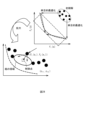
- a control point ( cf1 , cf2 ) in the rough region is set, and fm+1 is reflected in the evaluation function for searching for a solution, thereby controlling the solution search direction.
- fm+1 is reflected in the evaluation function for searching for a solution, thereby controlling the solution search direction.
- control points can be determined using the following procedure. First, Pareto solutions are extracted from the solutions obtained during the evolutionary computation. Next, the coordinates of the center of gravity of a random combination of m sets (the number of evaluation functions) of Pareto solutions are calculated. Next, each center of gravity is added to the Pareto solutions to find the hypervolume (HV), and the center of gravity with the maximum HV is detected as the control point. This is because, when the coordinates of the area with the coarsest solution are added to the Pareto solutions, the increase in HV is the largest.
- HV hypervolume
- HV is a performance index of Pareto solutions.
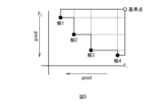
- HV represents the area or volume of the region formed by a certain reference point and a solution set obtained by an algorithm in the objective function space.
- the reference point can be set to (0,0) and the standardized values of each objective function can be used.
- the area shown in Figure 5 is the HV. The larger this HV is, the wider the solutions will be, so it can be determined that good results have been obtained.
- FIG. 6 is a diagram illustrating the result of a predetermined number of iterations of evolutionary calculation. It is assumed that four Pareto solutions are obtained by a predetermined number of iterations of evolutionary calculation.
- the coordinates of each Pareto solution are p1 , p2 , p3 , and p4 .
- the center of gravity c2,4 between p2 and p4 is calculated, and the center of gravity c1,2 between p1 and p2 is calculated, and so on.
- the HV is calculated from ( p1 , p2 , ..., p4 , c2,4 )
- the HV is calculated from ( p1 , p2 , ..., p4 , c1,2 ), and so on.
- the center of gravity c at which the HV is maximum is detected as the control point.
- FIG. 7(a) is a functional block diagram showing the overall configuration of an information processing device 100 according to the first embodiment.
- the information processing device 100 is, for example, a server for optimization processing. As illustrated in FIG. 7(a), the information processing device 100 functions as an evaluation function setting unit 10, an optimization execution unit 20, an intermediate progress recording unit 30, a result output unit 40, etc.
- FIG. 7(b) is a hardware configuration diagram of the information processing device 100. As illustrated in FIG. 7(b), the information processing device 100 includes a CPU 101, a RAM 102, a storage device 103, an input device 104, a display device 105, etc.
- the CPU (Central Processing Unit) 101 is a central processing unit.
- the CPU 101 includes one or more cores.
- the RAM (Random Access Memory) 102 is a volatile memory that temporarily stores the programs executed by the CPU 101 and the data processed by the CPU 101.
- the storage device 103 is a non-volatile storage device.
- a ROM Read Only Memory
- SSD solid state drive
- the storage device 103 stores an arithmetic program.
- the input device 104 is a device for a user to input necessary information, such as a keyboard or a mouse.
- the display device 105 is a display device that displays the results output by the result output unit 40 on a screen.
- Each part of the information processing device 100 is realized by the CPU 101 executing the arithmetic program.
- Each part of the information processing device 100 may be implemented using hardware such as a dedicated circuit.
- the evaluation function setting unit 10 sets a plurality of evaluation functions.
- the evaluation function setting unit 10 may set two evaluation functions, or may set three or more evaluation functions.
- the evaluation function setting unit 10 sets evaluation functions f 1 to f m for m objective functions.
- the optimization execution unit 20 executes optimization so that the evaluation function f for searching for a solution is optimized.
- the intermediate progress recording unit 30 records intermediate results as the optimization execution unit 20 executes optimization.
- the result output unit 40 outputs the results of the optimization executed by the optimization execution unit 20.
- Each evaluation function is, for example, the production completion time in a production process, the cost associated with production, etc. The shorter the production completion time, the better, and the lower the cost, the better.
- the optimization execution unit 20 sets an initial solution to a random value (step S2). There are multiple initial solutions.
- the initial solutions may be input by the user using the input device 104.
- step S3 the optimization execution unit 20 sets the (m+1)th evaluation function f m+1 (step S3). The details of step S3 will be described later.
- Step S4 is executed for the following reason.
- the evaluation function f is changed every time the control point is changed. Therefore, since the evaluation values from the (n-1)th generation and earlier that are referenced when calculating the solution for the nth evolutionary iteration are calculated using an evaluation function different from that for the nth generation, it is preferable to align the evaluation criteria. Therefore, by executing step S4, the evaluation function f for the solutions of generations (n-1) and below is matched to the evaluation function f when performing the nth generation evolutionary calculation.
- step S5 the optimization execution unit 20 performs generational evolution on the solutions obtained thus far (step S5).
- step S5 is executed the first time
- the initial solution is generationally evolved.
- step S5 is executed the second time onwards, the group of solutions that have not been selected so far and remain are the targets for evolution.
- step S6 judges whether the optimization has been completed. For example, it judges whether the number of generational evolutions has reached a predetermined number. If the judgment in step S6 is "No", execution is resumed from step S3. If the judgment in step S6 is "Yes", execution of the flowchart is terminated.
- FIG. 9 is a flowchart showing the details of step S3.
- the optimization execution unit 20 extracts Pareto solutions (step S11).
- step S11 is executed the first time, those that correspond to the Pareto solutions are extracted from the initial solutions.
- step S11 is executed the second or subsequent times, those that correspond to the Pareto solutions are extracted from the solutions that have been obtained up to that point.
- the optimization execution unit 20 calculates the center of gravity for m random combinations of the coordinates of the Pareto solutions extracted in step S11 (step S12).
- the optimization execution unit 20 adds the center of gravity to each coordinate of the Pareto solution to calculate the HV (step S13).
- the optimization execution unit 20 detects the center of gravity where HV is maximum as the control point (step S14).
- the optimization execution unit 20 reflects the distance f m+1 between the control point and each coordinate of the Pareto solution in the evaluation function f (step S15).
- the (m+1)th evaluation function can be set.
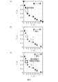
- FIGS. 10(a) to 10(c) are diagrams illustrating the detection of areas where the solution distribution is sparse when there are two evaluation functions. As illustrated in FIG. 10(a), assume that 10 Pareto solutions have been obtained. In this case, sparse areas have occurred. Next, as illustrated in FIG. 10(b), the centroid coordinates of a random combination (10 pairs) of the coordinates of the Pareto solutions are calculated. Next, as illustrated in FIG. 10(c), the centroid coordinates where HV is maximum can be detected as the control point.
- FIGS. 11(a) to 11(c) are diagrams illustrating the detection of areas where the solution distribution is sparse when there are three evaluation functions. As illustrated in FIG. 11(a), assume that 14 Pareto solutions have been obtained. In this case, sparse areas have occurred. Next, as illustrated in FIG. 11(b), the centroid coordinates of random combinations (50 pairs) of the coordinates of the Pareto solutions are calculated. Next, as illustrated in FIG. 11(c), the centroid coordinates where HV is maximum can be detected as the control point.
- the direction of the solution search is controlled according to the distribution of the Pareto solutions obtained, and the next generation of solutions is searched for. In this way, the direction of the solution search can be dynamically changed, making it possible to obtain Pareto solutions with high uniformity.
- control point condition a certain number of times
- the condition in (2) is met, it is decided to adopt it as a control point, this control point is stored and the process ends (3).
- the same control point appears consecutively for a certain number of times and does not satisfy the condition, its coordinates are registered in the NG list (4). Coordinates registered in the NG list are not used as control points.
- the center of gravity with the second largest HV is set as the control point candidate and the adoption conditions are judged (5). Next, the judgment result is obtained and the process returns to (3).
- FIG. 13 is a flowchart for the case where a wide gap occurs in the distribution of exact solutions that should have been obtained in step S3.
- the optimization execution unit 20 extracts Pareto solutions (step S31).
- step S31 is executed the first time, solutions that correspond to the Pareto solutions are extracted from the initial solutions.
- step S31 is executed the second or subsequent times, solutions that correspond to the Pareto solutions are extracted from the solutions that have been obtained up to that point.
- the optimization execution unit 20 calculates the center of gravity for m random combinations of the coordinates of the Pareto solutions extracted in step S31 (step S32).
- the optimization execution unit 20 adds the center of gravity to each coordinate of the Pareto solution to calculate the HV (step S33).
- the optimization execution unit 20 sets the control points based on the HV (step S34).
- the optimization execution unit 20 reflects the distance between the control point and each coordinate of the Pareto solution in the evaluation function f (step S35).
- the (m+1)th evaluation function fm+1 can be reflected in the evaluation function f.
- FIG. 14 is a flowchart showing the details of step S34. As shown in the example of FIG. 14, the optimization execution unit 20 sorts the HVs in descending order (step S41).
- the optimization execution unit 20 sets the centers of gravity as control point candidates in descending order of HV (step S42).
- step S43 the optimization execution unit 20 determines whether or not the control point candidate is present in the NG list (step S43). If the result of step S43 is "Yes,” the process is executed again from step S42. Therefore, the coordinates registered in the NG list will no longer be set as a control point.
- step S43 determines whether the control point candidate is the same as the previous generation (step S44).
- step S44 returns "No"
- the optimization execution unit 20 determines the control point candidate as the control point (step S45). Then, execution of the flowchart ends.
- step S44 returns "Yes," the optimization execution unit 20 counts the number of times the same control point appears consecutively (consecutive number) (step S46).
- the optimization execution unit 20 determines whether the number of consecutive occurrences counted in step S46 is equal to or greater than a threshold value (step S47).
- step S47 returns "No"
- the optimization execution unit 20 determines the control point candidate as the control point (step S48). Then, execution of the flowchart ends.
- step S47 returns "Yes," the optimization execution unit 20 adds the control point candidate to the NG list (step S49). Then, the process is executed again from step S42.
- Fig. 15(a) and Fig. 15(b) are diagrams comparing the search process for Pareto solutions.
- the number of generation evolutions was 240.
- Fig. 15(a) shows the result of searching for a solution without setting a control point.
- Fig. 15(b) shows the result of searching for a solution with a control point set.
- Fig. 15(b) shows that the bias in the distribution of solutions has been eliminated and the uniformity is higher.
- Figures 16(a) and 16(b) show a comparison of the search process for Pareto solutions. The number of generations of evolution was set to 720.
- Figure 16(a) shows the result of searching for a solution without setting a control point.
- Figure 16(b) shows the result of searching for a solution with a control point set. Compared to Figure 16(a), Figure 16(b) shows that the bias in the distribution of solutions has been eliminated and the uniformity is higher.
- Figures 17(a) and 17(b) show a comparison of the search process for Pareto solutions. The number of generations of evolution was set to 1,440.
- Figure 17(a) shows the result of searching for a solution without setting a control point.
- Figure 17(b) shows the result of searching for a solution with a control point set. Compared to Figure 17(a), Figure 17(b) shows that the bias in the distribution of solutions has been eliminated and the uniformity is higher.
- Figures 18(a) and 18(b) show a comparison of the search process for Pareto solutions. The number of generations of evolution was set to 2040.
- Figure 18(a) shows the result of searching for a solution without setting a control point.
- Figure 18(b) shows the result of searching for a solution with a control point set. Compared to Figure 18(a), Figure 18(b) shows that the bias in the distribution of solutions has been eliminated and the uniformity is higher.
- CR Cross Rate
- CR Cross Rate
- CR is calculated by dividing the area between the maximum and minimum values of the Pareto solutions for each objective function, and represents the proportion of solutions that exist within the divided area. The higher the CR, the more uniform the Pareto solutions that have been obtained.
- the CR in Figure 18(b) was 25% higher than the CR in Figure 18(a).
- Figure 19 shows the exact solution to this standard problem. As shown in Figure 19, there are large gaps in the distribution of exact solutions.
- Fig. 20(a) and Fig. 20(b) are diagrams comparing the search process for Pareto solutions.
- the number of generation evolutions was 760.
- Fig. 20(a) shows the result of searching for a solution without setting a control point.
- Fig. 20(b) shows the result of searching for a solution with a control point set.
- Fig. 20(b) shows that the bias in the distribution of solutions has been eliminated and the uniformity is higher.
- Figures 21(a) and 21(b) are diagrams comparing the search process for Pareto solutions. The number of generations of evolution was set to 1000.
- Figure 21(a) shows the result of searching for a solution without setting a control point.
- Figure 21(b) shows the result of searching for a solution with a control point set.
- Figure 21(b) shows that the bias in the distribution of solutions has been eliminated and the uniformity is higher.
- Figures 22(a) and 22(b) are diagrams comparing the search process for Pareto solutions. The number of generations of evolution was set to 1,370.
- Figure 22(a) shows the result of searching for a solution without setting a control point.
- Figure 22(b) shows the result of searching for a solution with a control point set. Compared to Figure 22(a), Figure 22(b) shows that the bias in the distribution of solutions has been eliminated and the uniformity is higher.
- the CR in Figure 22(b) was 18% higher than the CR in Figure 22(a).
- Figure 23 shows the relationship between the number of generations and GD (Generational Distance).
- GD represents the average value of the distance between each Pareto solution and the exact solution. The smaller the GD, the higher the convergence to the exact solution. As shown in Figure 23, when a control point is set, the GD is reduced by more than 99% from the initial value at the 1370th generation evolution, which indicates that all convergence occurred at that 1370th time.
- the multi-objective optimization is performed from the initial solution group, but the present invention is not limited thereto.
- the single-objective optimization may be performed for the initial solution by using each of the objective functions as an evaluation function to calculate a single-objective optimal solution having a better value than the initial solution, and the multi-objective optimization may be performed using the calculated single-objective optimal solution (Pareto solution) as a starting point.
- the Pareto solution is approached by the single-objective optimization with a small amount of calculation, and then the multi-objective optimization is performed, so that the amount of calculation required to reach the Pareto solution can be reduced.
- the optimization execution unit 20 is an example of an execution unit that executes a process of searching for a solution of the next generation by controlling the direction of the solution search according to the distribution of the obtained Pareto solutions when it repeats the process of searching for a solution by evolutionary computation based on an evaluation function that evaluates multiple objective functions.
Landscapes
- Engineering & Computer Science (AREA)
- Physics & Mathematics (AREA)
- General Physics & Mathematics (AREA)
- Mathematical Physics (AREA)
- Theoretical Computer Science (AREA)
- Pure & Applied Mathematics (AREA)
- Mathematical Optimization (AREA)
- Mathematical Analysis (AREA)
- Computational Mathematics (AREA)
- Data Mining & Analysis (AREA)
- General Engineering & Computer Science (AREA)
- Software Systems (AREA)
- Biophysics (AREA)
- Life Sciences & Earth Sciences (AREA)
- Health & Medical Sciences (AREA)
- Databases & Information Systems (AREA)
- Operations Research (AREA)
- Algebra (AREA)
- Evolutionary Biology (AREA)
- Computing Systems (AREA)
- Bioinformatics & Computational Biology (AREA)
- Bioinformatics & Cheminformatics (AREA)
- Molecular Biology (AREA)
- General Health & Medical Sciences (AREA)
- Evolutionary Computation (AREA)
- Computational Linguistics (AREA)
- Biomedical Technology (AREA)
- Artificial Intelligence (AREA)
- Genetics & Genomics (AREA)
- Physiology (AREA)
- Management, Administration, Business Operations System, And Electronic Commerce (AREA)
Priority Applications (4)
| Application Number | Priority Date | Filing Date | Title |
|---|---|---|---|
| EP23930472.8A EP4693111A1 (en) | 2023-03-29 | 2023-03-29 | Calculation program, calculation method, and information processing device |
| PCT/JP2023/012942 WO2024201834A1 (ja) | 2023-03-29 | 2023-03-29 | 演算プログラム、演算方法、および情報処理装置 |
| JP2025509447A JPWO2024201834A1 (https=) | 2023-03-29 | 2023-03-29 | |
| US19/336,727 US20260017338A1 (en) | 2023-03-29 | 2025-09-23 | Non-transitory computer-readable recording medium, calculation method and information processing device |
Applications Claiming Priority (1)
| Application Number | Priority Date | Filing Date | Title |
|---|---|---|---|
| PCT/JP2023/012942 WO2024201834A1 (ja) | 2023-03-29 | 2023-03-29 | 演算プログラム、演算方法、および情報処理装置 |
Related Child Applications (1)
| Application Number | Title | Priority Date | Filing Date |
|---|---|---|---|
| US19/336,727 Continuation US20260017338A1 (en) | 2023-03-29 | 2025-09-23 | Non-transitory computer-readable recording medium, calculation method and information processing device |
Publications (1)
| Publication Number | Publication Date |
|---|---|
| WO2024201834A1 true WO2024201834A1 (ja) | 2024-10-03 |
Family
ID=92903644
Family Applications (1)
| Application Number | Title | Priority Date | Filing Date |
|---|---|---|---|
| PCT/JP2023/012942 Ceased WO2024201834A1 (ja) | 2023-03-29 | 2023-03-29 | 演算プログラム、演算方法、および情報処理装置 |
Country Status (4)
| Country | Link |
|---|---|
| US (1) | US20260017338A1 (https=) |
| EP (1) | EP4693111A1 (https=) |
| JP (1) | JPWO2024201834A1 (https=) |
| WO (1) | WO2024201834A1 (https=) |
Cited By (1)
| Publication number | Priority date | Publication date | Assignee | Title |
|---|---|---|---|---|
| CN119357562A (zh) * | 2024-12-24 | 2025-01-24 | 北京炎黄国芯科技有限公司 | 集成电路高温环境下封装密封性评估方法及系统 |
Citations (5)
| Publication number | Priority date | Publication date | Assignee | Title |
|---|---|---|---|---|
| JP2002203228A (ja) | 2000-11-14 | 2002-07-19 | Honda R & D Europe (Deutschland) Gmbh | 多目的最適化方法 |
| JP2005285090A (ja) * | 2003-12-24 | 2005-10-13 | Yamaha Motor Co Ltd | 多目的最適化装置、多目的最適化方法および多目的最適化プログラム |
| JP2007172306A (ja) * | 2005-12-22 | 2007-07-05 | Yamaha Motor Co Ltd | 多目的最適化装置、多目的最適化方法および多目的最適化プログラム |
| JP2022077760A (ja) * | 2020-11-12 | 2022-05-24 | 富士通株式会社 | 情報処理プログラム、装置、及び方法 |
| JP2022106186A (ja) | 2021-01-06 | 2022-07-19 | 富士通株式会社 | 情報処理装置、情報処理方法、及び情報処理プログラム |
-
2023
- 2023-03-29 EP EP23930472.8A patent/EP4693111A1/en active Pending
- 2023-03-29 WO PCT/JP2023/012942 patent/WO2024201834A1/ja not_active Ceased
- 2023-03-29 JP JP2025509447A patent/JPWO2024201834A1/ja active Pending
-
2025
- 2025-09-23 US US19/336,727 patent/US20260017338A1/en active Pending
Patent Citations (5)
| Publication number | Priority date | Publication date | Assignee | Title |
|---|---|---|---|---|
| JP2002203228A (ja) | 2000-11-14 | 2002-07-19 | Honda R & D Europe (Deutschland) Gmbh | 多目的最適化方法 |
| JP2005285090A (ja) * | 2003-12-24 | 2005-10-13 | Yamaha Motor Co Ltd | 多目的最適化装置、多目的最適化方法および多目的最適化プログラム |
| JP2007172306A (ja) * | 2005-12-22 | 2007-07-05 | Yamaha Motor Co Ltd | 多目的最適化装置、多目的最適化方法および多目的最適化プログラム |
| JP2022077760A (ja) * | 2020-11-12 | 2022-05-24 | 富士通株式会社 | 情報処理プログラム、装置、及び方法 |
| JP2022106186A (ja) | 2021-01-06 | 2022-07-19 | 富士通株式会社 | 情報処理装置、情報処理方法、及び情報処理プログラム |
Cited By (1)
| Publication number | Priority date | Publication date | Assignee | Title |
|---|---|---|---|---|
| CN119357562A (zh) * | 2024-12-24 | 2025-01-24 | 北京炎黄国芯科技有限公司 | 集成电路高温环境下封装密封性评估方法及系统 |
Also Published As
| Publication number | Publication date |
|---|---|
| EP4693111A1 (en) | 2026-02-11 |
| US20260017338A1 (en) | 2026-01-15 |
| JPWO2024201834A1 (https=) | 2024-10-03 |
Similar Documents
| Publication | Publication Date | Title |
|---|---|---|
| US20060230018A1 (en) | Mahalanobis distance genetic algorithm (MDGA) method and system | |
| CN112597284B (zh) | 公司名称的匹配方法、装置、计算机设备及存储介质 | |
| CN113268936B (zh) | 一种基于多目标进化随机森林特征选择的关键质量特性识别方法 | |
| Falahiazar et al. | Determining the Parameters of DBSCAN Automatically Using the Multi-Objective Genetic Algorithm. | |
| CN115828011B (zh) | 基于大数据的数据分析方法和平台 | |
| US20260017338A1 (en) | Non-transitory computer-readable recording medium, calculation method and information processing device | |
| US7177863B2 (en) | System and method for determining internal parameters of a data clustering program | |
| Wahid et al. | An outlier detection algorithm based on KNN-kernel density estimation | |
| CN113806636A (zh) | 项目推荐方法、装置、电子设备和计算机存储介质 | |
| CN118469736A (zh) | 一种基于社区结构增强和多目标粒子群的社区发现方法 | |
| CN113869380B (zh) | 基于Kmeans聚类的数据分类方法、装置及电子设备 | |
| Aguilar-Ruiz | Class-specific feature selection for classification explainability | |
| Cai et al. | Fuzzy criteria in multi-objective feature selection for unsupervised learning | |
| US7542606B2 (en) | Use of Hausdorff distances in the earth mover linear program | |
| JP7488391B2 (ja) | 情報選択システム、情報選択方法及び情報選択プログラム | |
| CN113269217A (zh) | 基于Fisher准则的雷达目标分类方法 | |
| CN115758767B (zh) | 基于多基因多目标优化的发动机零部件选配方法及系统 | |
| Mohapatra et al. | Movie recommender system using improvised cuckoo search | |
| Chakraborty et al. | Selection of'K'in K-means clustering using GA and VMA | |
| CN116483030B (zh) | 一种三阶段混合算法求解柔性作业车间调度的方法 | |
| TWI912815B (zh) | 回歸模型之最佳化方法及其系統 | |
| CN115168237B (zh) | 一种跨项目软件缺陷预测方法及系统 | |
| Navajas-Guerrero et al. | A novel heuristic approach for the simultaneous selection of the optimal clustering method and its internal parameters for time series data | |
| Hamilton et al. | An evolutionary approach for constructing multi-stage classifiers | |
| Priya et al. | KMeans-NM-SalpEpi: Genetic Interactions Detection through K-Means Clustering with Nelder-Mead and Salp Optimization Techniques in Genome-Wide Association Studies |
Legal Events
| Date | Code | Title | Description |
|---|---|---|---|
| 121 | Ep: the epo has been informed by wipo that ep was designated in this application |
Ref document number: 23930472 Country of ref document: EP Kind code of ref document: A1 |
|
| ENP | Entry into the national phase |
Ref document number: 2025509447 Country of ref document: JP Kind code of ref document: A |
|
| WWE | Wipo information: entry into national phase |
Ref document number: 2025509447 Country of ref document: JP |
|
| WWE | Wipo information: entry into national phase |
Ref document number: 2023930472 Country of ref document: EP |
|
| NENP | Non-entry into the national phase |
Ref country code: DE |
|
| ENP | Entry into the national phase |
Ref document number: 2023930472 Country of ref document: EP Effective date: 20251029 |
|
| ENP | Entry into the national phase |
Ref document number: 2023930472 Country of ref document: EP Effective date: 20251029 |
|
| ENP | Entry into the national phase |
Ref document number: 2023930472 Country of ref document: EP Effective date: 20251029 |
|
| ENP | Entry into the national phase |
Ref document number: 2023930472 Country of ref document: EP Effective date: 20251029 |
|
| ENP | Entry into the national phase |
Ref document number: 2023930472 Country of ref document: EP Effective date: 20251029 |
|
| ENP | Entry into the national phase |
Ref document number: 2023930472 Country of ref document: EP Effective date: 20251029 |
|
| ENP | Entry into the national phase |
Ref document number: 2023930472 Country of ref document: EP Effective date: 20251029 |
|
| ENP | Entry into the national phase |
Ref document number: 2023930472 Country of ref document: EP Effective date: 20251029 |
|
| WWP | Wipo information: published in national office |
Ref document number: 2023930472 Country of ref document: EP |