WO2023248481A1 - データ符号化装置及びデータ符号化プログラム - Google Patents
データ符号化装置及びデータ符号化プログラム Download PDFInfo
- Publication number
- WO2023248481A1 WO2023248481A1 PCT/JP2022/025415 JP2022025415W WO2023248481A1 WO 2023248481 A1 WO2023248481 A1 WO 2023248481A1 JP 2022025415 W JP2022025415 W JP 2022025415W WO 2023248481 A1 WO2023248481 A1 WO 2023248481A1
- Authority
- WO
- WIPO (PCT)
- Prior art keywords
- axis
- data
- dependent data
- encoding
- approximation
- Prior art date
- Legal status (The legal status is an assumption and is not a legal conclusion. Google has not performed a legal analysis and makes no representation as to the accuracy of the status listed.)
- Ceased
Links
Images










Classifications
-
- G—PHYSICS
- G05—CONTROLLING; REGULATING
- G05B—CONTROL OR REGULATING SYSTEMS IN GENERAL; FUNCTIONAL ELEMENTS OF SUCH SYSTEMS; MONITORING OR TESTING ARRANGEMENTS FOR SUCH SYSTEMS OR ELEMENTS
- G05B19/00—Program-control systems
- G05B19/02—Program-control systems electric
- G05B19/18—Numerical control [NC], i.e. automatically operating machines, in particular machine tools, e.g. in a manufacturing environment, so as to execute positioning, movement or co-ordinated operations by means of program data in numerical form
- G05B19/404—Numerical control [NC], i.e. automatically operating machines, in particular machine tools, e.g. in a manufacturing environment, so as to execute positioning, movement or co-ordinated operations by means of program data in numerical form characterised by control arrangements for compensation, e.g. for backlash, overshoot, tool offset, tool wear, temperature, machine construction errors, load, inertia
-
- G—PHYSICS
- G05—CONTROLLING; REGULATING
- G05B—CONTROL OR REGULATING SYSTEMS IN GENERAL; FUNCTIONAL ELEMENTS OF SUCH SYSTEMS; MONITORING OR TESTING ARRANGEMENTS FOR SUCH SYSTEMS OR ELEMENTS
- G05B19/00—Program-control systems
- G05B19/02—Program-control systems electric
- G05B19/18—Numerical control [NC], i.e. automatically operating machines, in particular machine tools, e.g. in a manufacturing environment, so as to execute positioning, movement or co-ordinated operations by means of program data in numerical form
- G05B19/408—Numerical control [NC], i.e. automatically operating machines, in particular machine tools, e.g. in a manufacturing environment, so as to execute positioning, movement or co-ordinated operations by means of program data in numerical form characterised by data handling or data format, e.g. reading, buffering or conversion of data
-
- H—ELECTRICITY
- H03—ELECTRONIC CIRCUITRY
- H03M—CODING; DECODING; CODE CONVERSION IN GENERAL
- H03M7/00—Conversion of a code where information is represented by a given sequence or number of digits to a code where the same, similar or subset of information is represented by a different sequence or number of digits
- H03M7/30—Compression; Expansion; Suppression of unnecessary data, e.g. redundancy reduction
- H03M7/3059—Digital compression and data reduction techniques where the original information is represented by a subset or similar information, e.g. lossy compression
-
- H—ELECTRICITY
- H03—ELECTRONIC CIRCUITRY
- H03M—CODING; DECODING; CODE CONVERSION IN GENERAL
- H03M7/00—Conversion of a code where information is represented by a given sequence or number of digits to a code where the same, similar or subset of information is represented by a different sequence or number of digits
- H03M7/30—Compression; Expansion; Suppression of unnecessary data, e.g. redundancy reduction
- H03M7/60—General implementation details not specific to a particular type of compression
- H03M7/6041—Compression optimized for errors
Definitions
- the present disclosure relates to a data encoding device and a data encoding program.
- axis-dependent data that depends on the coordinate values of each axis of an industrial machine, such as the above-mentioned error amount, may have a white noise-like property with a uniform appearance frequency as a whole.
- it is difficult to compress data by entropy encoding because the above-mentioned small information entropy cannot be utilized.
- the present disclosure has been made in view of the above, and aims to provide a data encoding technique that can encode and compress axis-dependent data that depends on the coordinate values of each axis of an industrial machine.
- One aspect of the present disclosure is a data encoding device that encodes data, which includes a part of axis-dependent data that depends on the coordinate values of each axis of an industrial machine, and a part of the axis-dependent data that depends on the coordinate values of each axis of the industrial machine.
- the data encoding device includes a model approximation encoding unit that generates encoded axis-dependent data by encoding the axis-dependent data based on a linear combination model that is approximated as a linear combination of data.
- another aspect of the present disclosure is a data encoding program that encodes data, which includes a part of axis-dependent data that depends on the coordinate values of each axis of an industrial machine, and a part of the axis-dependent data that depends on the coordinate values of each axis of an industrial machine.
- a linear combination model that is approximated as a linear combination of each axis data; .
- FIG. 1 is a diagram showing the configuration of a data encoding device according to a first embodiment.
- FIG. 2 is a diagram showing an example of a text file containing only specific characters.
- FIG. 3 is a diagram illustrating an example of data expressed in a certain distribution of frequency of appearance of each value.
- FIG. 3 is a diagram showing data in which the frequency of appearance of each value is uniform. It is a figure which shows each axis error of the X-axis. It is a figure which shows each axis error of Y-axis. It is a figure showing the amount of errors in coordinate values (X 2 , Y 1 ).
- FIG. 7 is a diagram showing the amount of error when it cannot be represented by a linear combination of the errors of each axis.
- FIG. 9 is a partially enlarged view of FIG. 8.
- FIG. 3 is a diagram showing a bitmap image that visualizes an error map.
- FIG. 3 is a diagram showing an example of axis-dependent data.
- FIG. 12 is a diagram showing a linear combination model that approximates the axis-dependent data of FIG. 11 as a linear combination of errors in each axis of the industrial machine.
- FIG. 2 is a diagram showing the configuration of a data encoding device according to a second embodiment.
- FIG. 7 is a diagram showing axis-dependent data partitioned into a plurality of grid-like regions. It is a figure which shows an example of axis dependent data after division
- FIG. 3 is a diagram showing a bitmap image that visualizes an error map.
- FIG. 3 is a diagram showing an example of axis-dependent data.
- FIG. 12 is a diagram showing a linear combination model that approximates the axis-dependent data of FIG. 11
- FIG. 7 is a diagram showing the configuration of a data encoding device according to a third embodiment.
- 7 is a flowchart showing a procedure for dividing axis-dependent data by a dynamic programming processing unit.
- FIG. 7 is a diagram showing a divided section before expanding each axis data (each axis error) by one column in the positive X direction.
- FIG. 7 is a diagram showing divided sections after each axis data (each axis error) is expanded by one column in the positive X direction.
- FIG. 3 is a diagram showing the configuration of a data encoding device according to a fourth embodiment. It is a figure showing an approximation error (vector ⁇ [X][Y]).
- FIG. 7 is a diagram showing an approximation error (vector ⁇ [X][Y]) including an exceptional point larger than a predetermined tolerance.
- FIG. 6 is a diagram showing exceptional points that are excluded and retained because the approximation error (vector ⁇ [X][Y]) is larger than a predetermined tolerance.
- 3 is a flowchart showing the procedure of learning processing by the machine learning device 9.
- the data encoding device 1 encodes axis-dependent data that depends on the coordinate values of each axis of an industrial machine, such as the amount of error used for error correction of each axis of the industrial machine.
- This is a data encoding device that can compress data.
- axis-dependent data that depends on the coordinate values of each axis of an industrial machine may have a white noise-like property where the appearance frequency is uniform as a whole, so there may be a bias in the appearance frequency of values in the data, That is, it is difficult to compress data using conventional entropy encoding techniques that utilize small information entropy.
- the data encoding device 1 according to the present embodiment encodes and compresses axis-dependent data that depends on the coordinate values of each axis of an industrial machine.
- FIG. 1 is a diagram showing the configuration of a data encoding device 1 according to the first embodiment.
- the data encoding device 1 includes a model approximation encoding section 11.
- the model approximation encoding unit 11 generates encoded axis-dependent data by encoding the axis-dependent data based on the axis-dependent data and the linear combination model.
- a conventional data encoding technique will be explained.
- entropy encoding technique for example, an entropy encoding technique represented by a Huffman code is known.
- data is compressed by utilizing the bias in the frequency of occurrence of values in data, that is, the smallness of information entropy.
- FIG. 2 is a diagram showing an example of a text file containing only specific characters.
- FIG. 3 is a diagram showing an example of data represented by a certain distribution of appearance frequencies of each value.
- the horizontal axis indicates the bit value
- the vertical axis indicates the frequency of appearance of each value.
- a text file containing only 16 characters 0 to 9 and A to F as specific characters, as shown in Figure 2 normally requires 8 bits to represent one character, but due to entropy encoding, at most 4 bits per character. Since it can be expressed in bits, it is possible to compress the data by about half.
- data with uneven appearance frequencies as shown in Figure 3 can be processed by entropy encoding, which assigns short bit values to frequently occurring values, while assigning long bit values to less frequently occurring values. Compressible.
- FIG. 4 is a diagram showing data in which the appearance frequency of each value is uniform. Similar to FIGS. 2 and 3, in FIG. 4, the horizontal axis indicates bit values, and the vertical axis indicates the frequency of appearance of each value.
- White noise-like data with a uniform appearance frequency as shown in FIG. 4 cannot take advantage of the small information entropy described above, so it is difficult to compress the data by entropy encoding.
- examples of static error correction for each axis of industrial machinery include pitch error correction, straightness error correction, and three-dimensional error correction.
- Pitch error correction is correction of errors in the direction along the axial direction.
- Straightness error correction is correction of errors in a direction perpendicular to the axial direction.
- Three-dimensional error correction is correction of three-dimensional spatial errors.
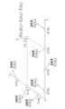
- FIG. 5 is a diagram showing each axis error on the X axis.
- Each axis error of the X axis is an error amount of each coordinate value measured when only the X axis is moved while the Y axis and the Z axis are fixed.
- the error amount of each coordinate value X 0 , X 1 , X 2 , and X 3 is represented by a vector having a different magnitude and direction.
- FIG. 6 is a diagram showing each axis error of the Y axis.
- Each Y-axis error is the amount of error in each coordinate value measured when only the Y-axis is moved while the X-axis and Z-axis are fixed.
- the error amount of each coordinate value Y 0 , Y 1 , and Y 2 is represented by a vector having a different magnitude and direction.
- each axis error is linearly independent. That is, assuming that the error amount (vector E[X 1 ]...[X L ]) at the coordinate values X 1 ,...X L is a linear combination of the errors in each axis, it is expressed as the following formula (1). is expressed in
- L represents the number of axes targeted for error correction.
- X l represents the lth correction target axis.
- FIG. 7 is a diagram showing the amount of error in the coordinate values (X 2 , Y 1 ).
- the error amount (vector E[X 2 ][Y 1 ]) in the coordinate value (X 2 , Y 1 ) is the error amount (vector E [X 2 ]) in the coordinate value X 2 and the error amount (vector E Y [Y 1 ]) of the coordinate value Y 1 can be regarded as a linear combination, and is expressed as in the following equation (2).
- each axis error is not linearly independent, and the error amount (vector E[X 1 ]...[X L ]) may be determined by the correlation of multiple axes.
- the error amount (vector E[X 1 ]...[ XL ]) is the correlation term (vector ⁇ [X 1 ]...[ XL ]). In some cases, it may not be expressed as a linear combination of errors in each axis.
- FIG. 8 is a diagram showing the amount of error when it cannot be represented by a linear combination of the errors of each axis.
- the error amount expressed by the above formula (1) is used as the error amount (vector E[X 1 ]...[X L ]). Instead, it is necessary to set the error amount to include the correlation term (vector ⁇ [X 1 ]...[X L ]) expressed by the above formula (3).
- the error amount hereinafter referred to as spatial error
- the control device for each space that has a correlation with the error amount and is corrected, it is called error correction for each space.
- the spatial error has the property that although it cannot be expressed as a linear combination of the errors of each axis as a whole, it can be regarded as a linear combination of errors of each axis locally, just like the errors of each axis. This is what the inventor discovered.
- FIG. 9 is a partial enlarged view of FIG . 8, and in the local area surrounded by the broken line in FIG .
- the spatial error can be expressed as a linear combination of errors in each axis.
- the spatial error (vector E[ X ][Y]) is calculated by the error of each axis (vector E It is expressed as the sum of This means that the spatial error (vector E[X][Y]) is the error amount in one row in the X-axis direction (vector E This means that it is possible to take out the error amount (vector E Y [Y]) and the error amount (vector E Y [Y]) in a row in the Y-axis direction and approximate it as a linear combination of these.
- the local area includes, for example, the central area of the movable range of the industrial machine.
- FIG. 10 is a diagram showing a bitmap image that visualizes the error map when the target axes for error correction are the X axis and the Y axis, and the RGB values of each pixel correspond to the error amount vector E. are doing. Further, the error amount (vector E[X][Y]) of each pixel is expressed as the sum of the vector E X [X] and the vector E Y [Y] according to the above equation (4).
- bitmap image shown in FIG. 10 has 10 ⁇ 10 pixels and is 374 bytes, it becomes 393 bytes when encoded using ZIP compression, which is a typical entropy encoding technique.
- ZIP compression which is a typical entropy encoding technique.
- the conventionally known entropy encoding has no compression effect and, in some cases, has the opposite effect of increasing the data size.
- the data encoding device 1 includes, for example, memories such as ROM (read only memory) and RAM (random access memory), and CPU (control processing) connected to each other via a bus. unit), operating means such as a keyboard, a display, and a communication control unit.
- memories such as ROM (read only memory) and RAM (random access memory)
- CPU control processing
- operating means such as a keyboard, a display, and a communication control unit.
- the data encoding device 1 may be provided, for example, in a numerical control device (CNC) corresponding to a control device for industrial machinery such as a machine tool or a robot, a robot control device, or the like. Alternatively, it may be provided in an external computer or the like so as to be able to communicate with these control devices.
- CNC numerical control device
- the model approximation encoding unit 11 included in the data encoding device 1 of the present embodiment converts a part of axis-dependent data that depends on the coordinate values of each axis of the industrial machine and axis-dependent data on each axis of the industrial machine (each The encoded axis-dependent data is generated by encoding the axis-dependent data based on a linear combination model that is approximated as a linear combination of axis errors).
- the axis-dependent data is input from, for example, the above-mentioned control device. Further, the linear combination model is stored in the storage unit of the data encoding device 1, for example.
- each axis of an industrial machine means, for example, each axis of a machine tool, that is, the X axis, Y axis, and Z axis.
- axis-dependent data includes, for example, the installation error amount of relatively large workpieces whose displacement varies depending on the coordinate value due to the influence of deflection due to their own weight. It will be done.
- error amounts and workpiece installation error amounts are both data that depend on the coordinate values of each axis of the industrial machine.
- model approximation encoding using a linear combination model by the model approximation encoding unit 11 of this embodiment will be described in detail with reference to FIGS. 11 and 12.
- FIG. 11 is a diagram showing an example of axis-dependent data.
- the example shown in FIG. 11 shows axis-dependent data when the target axes for error correction etc. are two axes, the X axis and the Y axis.
- the axis-dependent data shown in FIG. 11 is, for example, the amount of error in each axis of industrial machinery, etc., and is the axis-dependent data of a certain local area in the axis-dependent data in which there is no bias in the frequency of occurrence of values in the data as a whole. This is axis-dependent data that can be approximated by a linear combination model.
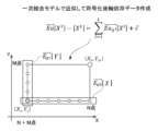
- the example of axis-dependent data shown in FIG. 11 has a total of N ⁇ M points of each axis data (each axis error).
- FIG. 12 is a diagram showing a linear combination model that approximates the axis-dependent data of FIG. 11 as a linear combination of errors in each axis of the industrial machine.
- the error amount (vector E[X 1 ]...[X L ]) follows the model expressed by the above formula (3), and as a whole, the correlation term (vector ⁇ [X 1 ]... Even if the influence of [X L ]) is considered to be strong, it is thought that locally there is a region that can be approximated by the linear combination model expressed by the above formula (1). For such an approximable region, as shown in FIG. The amount of error can be expressed.
- each axis data (each axis error) after approximation has a total of N+M points, indicating that axis-dependent data can be compressed.
- Equation (8) L represents the number of axes to be corrected for error
- Xl represents the lth axis to be corrected
- Nl represents the number of error amount points of the lth axis to be corrected.
- X represents a one-dimensional axial space
- x represents an element belonging to the space.
- p is any value from 1 to L.
- x 3 means a certain possible value of axis X 3 .
- the approximate model (vector Ea[X 1 ]...[X L ]) as the linear combination model is an evaluation function expressed by the following equation (9).
- the evaluation function J is calculated by combining the original error amount before approximation (vector E[X 1 ]...[X L ]) and the error amount after approximation (vector Ea[X 1 ]...[X L ]), and the approximate model as the above-mentioned linear combination model (vector Ea[X 1 ] ⁇ ...[ XL ]) is determined.
- the approximate model as a linear combination model determined in this manner is stored, for example, in the storage unit of the data encoding device 1, and is used for model approximation encoding by the model approximation encoding unit 11.
- a part of the axis-dependent data that depends on the coordinate values of each axis of the industrial machine and the axis-dependent data are linearly combined with each axis data (each axis error) of the industrial machine.
- a model approximation encoding unit 11 is provided which generates encoded axis-dependent data by encoding axis-dependent data based on the linear combination model to be approximated.
- axis-dependent data such as the amount of error in each axis of industrial machinery, which has a uniform appearance frequency as a whole and may resemble white noise, has a bias in the frequency of occurrence of values in the data, that is, information entropy.
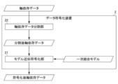
- FIG. 13 is a diagram showing the configuration of a data encoding device 2 according to the second embodiment.
- the data encoding device 2 according to the second embodiment differs from the data encoding device 1 according to the first embodiment in that it includes an axis-dependent data dividing section 22.
- the model approximation encoding unit 21 of the second embodiment executes model approximation encoding based on the divided axis-dependent data generated by dividing the axis-dependent data into a plurality of pieces and the above-mentioned linear combination model. This is different from the model approximation encoding unit 11 of the first embodiment in that.
- the configuration other than these differences is the same as the first embodiment.
- the data encoding device 1 performs a linear combination of each axis data (each axis error) and a part of the axis dependent data that has a uniform appearance frequency as a whole and may resemble white noise. It can be considered as performing a model approximation encoding of a linear combination model.
- the data encoding device 2 according to the present embodiment actively divides the axis-dependent data into multiple regions, thereby making it possible to treat each axis data (each axis error) as a linear combination. This method generates a plurality of possible regions, thereby making it possible to execute model approximation coding of a linear combination model more reliably.
- the axis-dependent data dividing unit 22 divides the axis-dependent data and generates a plurality of divided axis-dependent data.
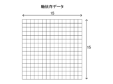
- FIG. 14 is a diagram showing axis-dependent data partitioned into a plurality of grid-like regions.
- the axis-dependent data input to the data encoding device 2 is divided into a plurality of grid-like regions according to each axis data (each axis error) on each coordinate value, for example. Ru.
- the axis-dependent data dividing unit 22 divides the axis-dependent data into a plurality of pieces, for example, along these sections.
- the method for dividing axis-dependent data by the axis-dependent data dividing unit 22 is not particularly limited, but the axis-dependent data is It is preferable to divide the In particular, it is preferable that the axis-dependent data dividing unit 22 divides the axis-dependent data into a plurality of regions that can best be approximated (compressed).
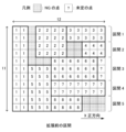
- FIG. 15 is a diagram showing an example of axis-dependent data after division.
- the axis-dependent data input to the data encoding device 2 is divided into five division sections 1 to 5 by the axis-dependent data dividing section 22.
- each data within each of these five divided sections 1 to 5 corresponds to the axis-dependent data after division
- each of these axis-dependent data after division is regarded as a linear combination of each axis data (each axis error). It is possible to perform model approximation encoding of a linear combination model by the model approximation encoding unit 21, which will be described later.
- the model approximation encoding unit 21 generates encoded axis-dependent data based on the plurality of divided axis-dependent data and the linear combination model. As described above, within each of the plurality of divided sections 1 to 5, the axis-dependent data can be regarded as a linear combination of each axis data (each axis error). Therefore, the model approximation encoding unit 21 generates model-approximated and compressed encoded axis-dependent data by executing model approximation encoding of the linear combination model for each axis-dependent data after division.
- the data encoding device 2 is provided with an axis-dependent data dividing unit 22 that divides axis-dependent data and generates a plurality of divided axis-dependent data. Furthermore, the model approximation encoding unit 21 is configured to generate encoded axis-dependent data based on the plurality of divided axis-dependent data and the linear combination model. As a result, according to this embodiment, by actively dividing the axis-dependent data into a plurality of regions, it is possible to generate a plurality of regions that can be regarded as a linear combination of each axis data (each axis error). By performing model approximation coding of a linear combination model for each region, axis-dependent data, which was difficult to compress in the past, can be more reliably compressed.
- FIG. 16 is a diagram showing the configuration of a data encoding device 3 according to the third embodiment.
- the data encoding device 3 according to the third embodiment differs from the axis-dependent data dividing unit 22 in the second embodiment in the configuration of the axis-dependent data dividing unit 32. It differs from the form. The configuration other than this difference is the same as the second embodiment.
- the method of dividing axis-dependent data is not particularly limited, but in the data encoding device 3 according to the third embodiment, dynamic programming is used. split axis-dependent data. That is, by using dynamic programming, it is possible to perform optimal division of axis-dependent data, and the axis-dependent data can be best approximated and compressed.
- the axis-dependent data division section 32 of this embodiment includes a dynamic programming processing section 33.
- the dynamic programming processing unit 33 generates optimal post-division axis-dependent data by executing dynamic programming.
- the dynamic programming processing unit 33 includes, as functional units for executing dynamic programming, an optimality evaluation unit 34 after model approximation coding, an axis-dependent data partial division unit 35, and a partial division unit 35 for axis-dependent data. and an axis-dependent data optimization result combination unit 36.
- Dynamic programming is a general-purpose algorithm for solving optimization problems. Dynamic programming is an algorithm that has the following two characteristics. The first feature is that it is solved recursively. That is, it is characterized by dividing into small-scale subproblems, recursively optimizing the subproblems, and combining the optimization results of the subproblems to obtain a solution to the larger-scale original problem. The second feature is that the processing load can be reduced by recording the optimization results. In other words, in the process of recursively solving problems, the same problem may appear many times, but in order to omit calculations for problems that have already been solved, the optimization results of the problem once solved are recorded. It is characterized by its ability to be stored and reused.
- the dynamic programming processing unit 33 of this embodiment includes a model approximation coding post-optimality evaluation unit 34 as a means for evaluating the optimality of the result. That is, the model approximation-encoded optimality evaluation unit 34 evaluates the optimality of the encoded axis-dependent data.
- the optimality of encoded axis-dependent data can be evaluated based on, for example, whether the approximation error amount after model approximation encoding is within a predetermined constraint tolerance.
- the approximation error amount after model approximation encoding is the original error amount before model approximation encoding described in the above-mentioned first embodiment, and the model approximation error amount, as described in detail in the fourth embodiment below. This is the difference from the amount of error after encoding.
- the constraint tolerance may be, for example, an approximation error tolerance or an allowable number of data points exceeding the approximation error tolerance.
- the dynamic programming processing unit 33 of this embodiment also includes an axis-dependent data partial division unit 35 as a means for dividing a problem into partial problems.
- the axis-dependent data partial division unit 35 divides the axis-dependent data into a plurality of parts to generate partial axis-dependent data.
- the axis-dependent data partial division unit 35 divides the axis-dependent data into predetermined specified sections according to a predetermined division criterion stored in advance, and then divides the axis-dependent data into sections in the + direction or - direction of each axis such as the X axis or the Y axis.
- the axis-dependent data is divided into multiple parts by optimizing downscaling one point in each direction. The division of axis-dependent data by the axis-dependent data partial division unit 35 will be described in detail later.
- the dynamic programming processing unit 33 of this embodiment also includes a partial axis-dependent data optimization result combination unit 36 as a means for combining (combining) the optimization results of partial problems.
- the partial axis-dependent data optimization result combination unit 36 generates optimal post-division axis-dependent data by expanding and combining the partial axis-dependent data.
- the partial axis-dependent data optimization result combining unit 36 for example, divides the partial axis-dependent data generated by dividing the axis-dependent data by the axis-dependent data partial dividing unit 35 into the X-axis, Y-axis, etc. Optimize by expanding one point in each axis in the + direction or - direction. The generation of optimal divided axis-dependent data by the partial axis-dependent data optimization result combination unit 36 will be described in detail later.
- axis-dependent data is divided into sections by the dynamic programming processing unit 33, divided axis-dependent data as shown in FIG. 15, for example, is obtained.
- the approximation error of each error amount is kept within the constraint tolerance when each region of the divided interval is approximated by the above-mentioned approximation model.
- points where the approximation error does not fall within the constraint tolerance are allowed up to the constraint tolerance. Nevertheless, the number of points that cannot be approximated and do not satisfy the constraints is minimized. As a result, the number of data points, for example, 225 can be compressed to 92 points, and the data size can be reduced.
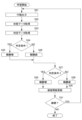
- FIG. 17 is a flowchart showing the procedure for dividing axis-dependent data by the dynamic programming processing unit 33.
- the division of the axis-dependent data by the dynamic programming processing unit 33 is performed by recursively searching for an optimal division section of the axis-dependent data using dynamic programming.
- step S1 the axis-dependent data is divided into predetermined designated sections. However, if the area has already been subjected to division processing of axis-dependent data by the dynamic programming processing unit 33, the held processing results may be reflected in this step. After that, the process advances to step S2.
- step S2 an approximate model of the region within the designated section (designated region) divided into sections in step S1 is generated. Specifically, for each specified region, an approximate model (vector Ea[X 1 ]...[X L ]) as a linear combination model described in the first embodiment is generated. After that, the process advances to step S3.
- step S3 it is determined whether the approximate model of the designated area generated in step S2 satisfies the all-point constraint.
- the constraints include whether the approximation errors of all points are within the allowable value, or whether the points whose approximation errors are not within the allowable value are within the allowable number of points. If this determination is YES, it is assumed that the axis-dependent data has been optimally divided and that the optimal axis-dependent data after division has been obtained, and the process ends. On the other hand, if this determination is NO, the process advances to step S4.
- n is set to an initial value of 1.
- the value of n represents each axis.
- the process advances to step S5.
- step S5 it is determined whether n is greater than L.
- L is the number of axes in the designated section of axis-dependent data. For example, if there are two axes, the X axis and the Y axis, L is 2. If this determination is YES, the process advances to step S11. On the other hand, if this determination is NO, the process advances to step S6.
- steps S6 to S10 is performed when n is less than or equal to L, and when there are two axes, the X and Y axes, if n is 1, it means processing for the X axis, and if n is 2, it means processing for the X axis. If it exists, it means processing for the Y axis.
- step S6 the axis-dependent data is divided into specified sections narrowed by one row of each axis data (each axis error) in the X n positive direction from the specified section in step S1. That is, a new section division is performed in which each axis data (each axis error) is reduced by one column in the Xn positive direction.
- the X n positive direction means the X-axis positive direction when n is 1.
- the result is output as an optimization result nP. When n is 1, the optimization result 1P is output. After that, the process advances to step S7.
- step S7 the optimization result nP obtained in step S6 is expanded by one column of each axis data (each axis error) in the Xn positive direction. The result is output as the optimization result nP + .
- n 1
- the optimization result 1P + is output. Since n can range from 1 to L, this step yields optimization results 1P to LP + .
- the process advances to step S8.
- step S8 the axis-dependent data is divided into specified sections narrowed by one row of each axis data (each axis error) in the negative direction of Xn from the specified section in step S1. That is, a new section division is performed in which each axis data (each axis error) is reduced by one column in the negative direction of Xn .
- the X n negative direction means the negative direction of the X axis when n is 1.
- the result is output as an optimization result nM. When n is 1, an optimization result of 1M is output. After that, the process advances to step S9.
- step S9 the optimization result nM obtained in step S8 is expanded by one column of each axis data (each axis error) in the negative direction of Xn .
- the result is output as the optimization result nM + .
- n 1
- an optimization result of 1M + is output. Since n can range from 1 to L, this step results in optimization results of 1M to LM + .
- the process advances to step S10.
- step S10 n is increased by 1. After that, the process returns to step S5.
- step S11 is performed when n is larger than L, and when the number of axes is two, the X-axis and the Y-axis, after the processing for the X-axis and Y-axis is completed in steps S6 to S10. It is processing.
- step S11 among the optimization results 1P to LP + and 1M to LM + obtained in steps S6 to S10, the one with the smallest number of non-approximable points is output. That is, for each of the optimization results 1P to LP + and 1M to LM + , the number of unapproximable points where the approximate model generated in step S3 does not satisfy the above constraints is calculated, and the number of unapproximable points is the smallest and best approximated. The data with the most compressed data is output, and the process ends.
- FIG. 18 is a diagram showing divided sections before each axis data (each axis error) is expanded by one column in the positive X direction.
- FIG. 19 is a diagram showing divided sections after each axis data (each axis error) is expanded by one column in the X positive direction. In FIGS. 18 and 19, different numbers are assigned to each divided section.
- sections 1 to 5 are extracted as continuous sections that appear at the end in the positive X direction of the section before each axis data (each axis error) is expanded by one column.
- each of the extracted sections 1 to 5 is expanded by one column of each axis data (each axis error) to generate expanded sections 1 to 5 as shown in FIG.
- post-expansion sections 1 to 5 it is checked whether the above-mentioned approximate model satisfies the above-mentioned constraints. If the constraints are satisfied, the section after expansion is set as a new section. In the example shown in FIG. 19, post-expansion sections 1 and 4 satisfy the constraints and are therefore set as new sections.
- the extended section will be an undetermined section.
- the extended section since post-expansion section 2 does not satisfy the constraints, it is set as an undetermined section.
- the undetermined section has a certain area (for example, 2 ⁇ 2) or more, it is checked whether the above-mentioned approximate model satisfies the above-mentioned constraints. In the example shown in FIG. 19, this determination is performed because post-expansion section 3 has a fixed area (for example, 2 ⁇ 2) or more. Until then, the expanded section will also be considered an undetermined section.
- a certain area for example, 2 ⁇ 2 or more
- the section before expansion is an NG section, that is, a section that does not satisfy the constraints and cannot be approximated
- the section for expansion is set as an undetermined section.
- post-expansion section 5 corresponds to this, and is therefore set as an undetermined section.
- Such an interval may ultimately be an NG interval, that is, an interval that does not satisfy the constraints and cannot be approximated.
- the data encoding device 3 is provided with a dynamic programming processing unit 33 that generates optimal post-division axis-dependent data by executing dynamic programming.
- the dynamic programming processing unit 33 also includes an optimality evaluation unit 34 that evaluates the optimality of the axis-dependent data after encoding, and an optimality evaluation unit 34 that divides the axis-dependent data into a plurality of parts to generate partial axis-dependent data. It is comprised of a partial division section 35 and an optimization result combination section 36 that combines optimization results of partial axis-dependent data to generate optimal post-division axis-dependent data.
- the axis-dependent data can be divided into optimal divided axis-dependent data that can be compressed by reducing the number of data to the greatest extent possible, so that it can be regarded as a linear combination of each axis data (each axis error).
- FIG. 20 is a diagram showing the configuration of a data encoding device 4 according to the fourth embodiment.
- the data encoding device 4 according to the fourth embodiment differs from the model approximation encoding unit 11 of the first embodiment in that the model approximation encoding unit 41 includes an approximation error calculation unit 42. differ.
- the data encoding device 4 according to the fourth embodiment differs from the data encoding device 1 according to the first embodiment in that it includes an approximate error encoding section 43.
- the configuration other than these differences is the same as the first embodiment.
- the approximation error calculation unit 42 calculates the amount of approximation error.
- the approximation error calculation unit 42 of this embodiment is provided in the model approximation encoding unit 41, and calculates an approximation error amount when the axis-dependent data is encoded by model approximation. This approximation error amount will be explained in detail later.
- the approximation error encoding unit 43 encodes the approximation error amount to generate an encoded approximation error amount.
- the amount of approximation error calculated by the approximation error calculation unit 42 is biased in the appearance frequency of values in the data, as will be described later, and the information entropy is often small. It is possible to compress. Alternatively, data may be compressed by encoding by model approximation encoding of a linear combination model executed by the model approximation encoding unit 41.
- vector E[X 1 ]...[ XL ] is the original error amount before model approximation
- vector Ea[X 1 ]...[ XL ] is the amount of error before model approximation. This is the amount of error after. From this formula (10), it can be seen that these differences are approximation errors (vector ⁇ [X 1 ]...[X L ]).
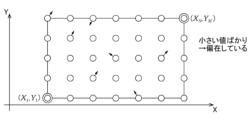
- FIG. 21 is a diagram showing the approximation error (vector ⁇ [X][Y]).
- the approximation error (vector ⁇ [X][Y]) has only small values unevenly distributed, and the frequency distribution of the values is also unevenly distributed. Therefore, data can be compressed by encoding the approximation errors (vectors ⁇ [X 1 ]...[X L ]).
- the approximation error (vector ⁇ [X 1 ]...[X L ]) may be encoded by the linear combination model approximation encoding described above, and the approximation error may be encoded by entropy encoding represented by the conventionally known Huffman code.
- the error (vector ⁇ [X 1 ]...[X L ]) may be encoded.
- the approximation error (vector ⁇ [X 1 ]...[ XL ]) and combining it with the approximate model (vector Ea[X 1 ]...[ XL ])
- the original error amount ( The vectors E[X 1 ]...[X L ]) can be compressed and reproduced without loss, and the total data size can also be reduced.
- the model approximation encoding unit 41 is provided with an approximation error calculation unit 42 that calculates the amount of approximation error. Furthermore, the data encoding device 4 is configured to further include an approximation error encoding unit 43 that encodes the approximation error amount and generates an approximation error amount after encoding.
- an approximation error encoding unit 43 that encodes the approximation error amount and generates an approximation error amount after encoding.
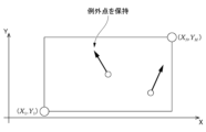
- FIG. 22 is a diagram showing the configuration of a data encoding device 5 according to the fifth embodiment.
- the data encoding device 5 according to the fifth embodiment differs from the data encoding device 4 according to the fourth embodiment in that it further includes an approximation error removal unit 53 having a predetermined tolerance or more.
- this embodiment is different from the approximation error encoding unit 43 of the fourth embodiment in that the approximation error encoding unit 54 encodes an approximation error amount within a predetermined tolerance.
- the configuration other than these differences is the same as the fourth embodiment.
- the approximation error removal unit 53 generates an approximation error amount within a predetermined tolerance by removing an approximation error amount that exceeds a predetermined tolerance from the approximation error amount.
- FIG. 23 is a diagram showing an approximation error (vector ⁇ [X][Y]) including an exceptional point larger than a predetermined tolerance.
- the approximation error (vector ⁇ [X][Y]) which is the difference between the original error amount before model approximation encoding and the error amount after model approximation encoding, has the following: Exception points larger than a predetermined tolerance may be included. In this embodiment, this exceptional point is removed by the approximation error removal unit 53.
- FIG. 24 is a diagram showing exceptional points that are excluded and retained because the approximation error (vector ⁇ [X][Y]) is larger than a predetermined tolerance.
- the approximation error removal unit 53 may separately retain the exceptional points where the approximation error is larger than the predetermined tolerance, that is, the approximation error amount that exceeds the predetermined tolerance, which is removed from the approximation error amount.
- axis-dependent data such as the original error amount can be compressed and reproduced without loss.
- the predetermined tolerance examples include an approximation error tolerance and a predetermined number of data points (tolerance) that exceed the approximation error tolerance.
- the approximation error removal unit 53 converts points exceeding a preset approximation error tolerance value or a predetermined number of points out of the points exceeding the approximation error tolerance value into an approximation error (vector ⁇ [X][Y]). Exclude from Note that the predetermined tolerance may include 0.
- the approximation error encoding unit 54 encodes the approximation error amount within a predetermined tolerance to generate an encoded approximation error amount. That is, in encoding the approximation error (vector ⁇ [X 1 ]...[X L ]), the approximation error encoding unit 54 of this embodiment excludes points where the approximation error is larger than a predetermined tolerance, and then , perform the encoding.
- the approximation error after excluding points larger than the predetermined tolerance from the approximation error amount becomes more biased and the information entropy becomes smaller, so that the data compression effect becomes more effective by encoding. It increases. Further, for example, the data size after encoding can be further reduced by retaining only the points where the approximation error is larger than a predetermined tolerance and not retaining the other approximation error amounts. Even in that case, it is possible to guarantee that the entire approximation error falls within the tolerance.
- the data encoding device 5 further includes an approximation error removal unit 53 that generates an approximation error amount within a predetermined tolerance by removing an approximation error amount exceeding a predetermined tolerance from the approximation error amount.
- the approximation error encoding unit 54 is configured to encode an approximation error amount within a predetermined tolerance to generate an approximation error amount after encoding.
- FIG. 25 is a diagram showing the configuration of a data encoding device 6 according to the sixth embodiment.
- the data encoding device 6 according to this embodiment differs from the data encoding device 1 according to the first embodiment in that it further includes a model approximation-encoded data encoding section 62.
- this embodiment has the same configuration as the first embodiment.
- the model approximation encoded data encoding unit 62 encodes the model approximation encoded axis-dependent data. In other words, in this embodiment, the model approximation encoded data encoding unit 62 executes re-encoding of axis-dependent data after model approximation encoding.
- the data encoding device 6 further includes a model approximation encoded data encoding unit 62 that encodes the encoded axis-dependent data.
- the encoded axis-dependent data is further encoded by the model approximation encoded data encoder 62, so that the data size can be further reduced.
- FIG. 26 is a diagram showing the configuration of a data encoding device 7 according to the seventh embodiment.
- the data encoding device 7 according to the present embodiment includes a learning result acquisition unit that acquires the reinforcement learning results by the machine learning device 9 instead of dynamic programming, and utilizes the learning results.
- This differs from the data encoding device 3 according to the third embodiment in that the axis-dependent data is divided into sections. The configuration other than this difference is the same as the third embodiment.
- the machine learning device 9 executes reinforcement learning for optimal division processing of axis-dependent data.
- the machine learning device 9 as an agent acquires axis-dependent data such as the error amount of industrial machinery as the state of the environment, and selects certain axis-dependent data after division as an action. Then, the environment changes based on the action. With this change in environment, the number of unapproximable points and the amount of data after approximation, which are obtained by model approximation coding of the axis-dependent data after division, are obtained as determination data.
- the machine learning device 9 as an agent learns the optimal post-division axis-dependent data for selecting a better action, that is, making a decision.
- the machine learning device 9 as an agent learns to select an action that maximizes the total reward over the future.
- Q learning which is a method of learning the value Q(s, a) of selecting action a under a certain environmental state s
- Q-learning in a certain state s, from among possible actions a, the action a with the highest value Q(s, a) is selected as the optimal action.
- the machine learning device 9 as an agent selects various actions a under a certain state s, and selects a better action for the action a at that time based on the reward given. We will learn the correct value Q(s, a).
- E[ ] represents the expected value
- t is time
- ⁇ is a parameter called a discount rate which will be described later
- r t is the reward at time t
- ⁇ is the sum at time t.
- the expected value in this equation is the expected value when the state changes according to the optimal action.
- reinforcement learning is performed while exploring by performing various actions.
- Such an update formula for the value Q(s, a) can be expressed, for example, as shown in Equation (11) below.
- s t represents the state of the environment at time t
- a t represents the behavior at time t. Due to the action a t , the state changes to s t+1 . r t+1 represents the reward obtained by changing the state.
- the term with max is the Q value when action a with the highest Q value known at that time is selected under state s t+1 multiplied by ⁇ .
- ⁇ is a parameter satisfying 0 ⁇ 1 and is called a discount rate.
- ⁇ is a learning coefficient and is in the range of 0 ⁇ 1.
- the above formula (11) represents a method of updating the value Q(s t , at ) of the action a t in the state s t based on the reward r t+1 returned as a result of the trial a t .
- This update formula shows that the value of the best action max a Q(s t +1 , a ) in the next state s t +1 due to action a t is greater than the value Q(s t , a t ) of action a t in state s t. If it is larger, Q(s t , a t ) is increased, and if it is smaller, Q(s t , at ) is decreased.
- Q learning there is a method of creating a table of Q(s, a) for all state-action pairs (s, a) and performing learning.
- the number of states is too large to obtain the values of Q(s, a) for all state-action pairs, and it may take a long time for Q-learning to converge.
- DQN Deep Q-Network
- the value of value Q (s, a) can be calculated by configuring value function Q using an appropriate neural network, adjusting the parameters of the neural network, and approximating value function Q with an appropriate neural network. It may be calculated.
- DQN it is possible to shorten the time required for Q learning to converge.
- non-patent literature "Human-level control through deep reinforcement learning", by Volodymyr Mnih1 [online], [searched on January 17, 2017], Internet ⁇ URL: http://files.davidqiu .com/research/nature14236.pdf> has a detailed description.
- the machine learning device 9 includes a state observation section 91, a determination data acquisition section 92, a learning section 93, and a decision making section 94, as shown in FIG. Be prepared. Further, the learning section 93 includes a remuneration calculation section 95 and a value function updating section 96.
- the state observation unit 91 acquires axis-dependent data as state data from the data encoding device 7. Further, the state observation unit 91 outputs the acquired axis-dependent data to the learning unit 93.
- the determination data acquisition unit 92 acquires the number of non-approximation points and the amount of data after approximation obtained by model approximation encoding of the post-division axis-dependent data from the data encoding device 7 as determination data.
- the divided axis-dependent data is obtained by dividing the axis-dependent data into predetermined specified sections according to a predetermined division criterion stored in advance. Further, the determination data acquisition unit 92 outputs the acquired number of unapproximable points and the amount of data after approximation to the learning unit 93.
- the reward calculation unit 95 of the learning unit 93 calculates the reward based on the acquired axis-dependent data, the number of points that cannot be approximated, and the amount of data after approximation. Specifically, the reward calculation unit 95 increases the reward when the number of points that cannot be approximated decreases, and decreases the reward when the number of points that cannot be approximated increases. Further, the reward calculation unit 95 increases the reward when the amount of data after approximation decreases, and decreases the reward when the amount of data after approximation increases.
- the value function updating unit 96 of the learning unit 93 calculates the number of unapproximable points, the amount of data after approximation, and the reward value obtained by model approximation encoding of the axis-dependent data as state data and the axis-dependent data after division as judgment data.
- the stored value function is updated by performing the above-mentioned Q learning based on .
- the value function stored by the value function update unit 96 can be shared by, for example, a plurality of machine learning devices that are communicably connected to each other.
- the decision making unit 94 obtains the updated value function from the value function updating unit 96. Furthermore, the decision-making unit 94 outputs the optimal post-division axis-dependent data to the data encoding device 7 as a behavior output based on the acquired value function.
- FIG. 27 is a flowchart showing the procedure of learning processing by the machine learning device 9.
- step S21 first, the machine learning device 9 outputs the divided axis-dependent data to the data encoding device 7 as a behavioral output.
- the divided axis-dependent data output in this step is obtained by dividing the axis-dependent data into predetermined specified sections according to a predetermined division criterion stored in advance.
- the data encoding device 7 generates the number of unapproximable points and the amount of data after approximation by executing model approximation encoding on the axis-dependent data after division. After that, the process advances to step S22.
- step S22 the machine learning device 9 acquires axis-dependent data as state data from the data encoding device 7. After that, the process advances to step S23.
- step S23 the machine learning device 9 acquires the number of unapproximable points after model approximation encoding and the amount of data after approximation of the axis-dependent data after division, which were generated in step S21, from the data encoding device 7 as determination data. After that, the process advances to step S24.
- step S24 as determination condition 1, it is determined whether or not the number of unapproximable points has decreased when the data encoding device 7 executes model approximation encoding on the divided axis-dependent data. If this determination is YES, the process proceeds to step S25 and the reward is increased. On the other hand, if this determination is NO, the process proceeds to step S26 and the reward is decreased. After that, the process advances to step S27.
- step S27 as determination condition 2, it is determined whether the amount of data after model approximation encoding is reduced when the data encoding device 7 executes model approximation encoding on the axis-dependent data after division. . If this determination is YES, the process proceeds to step S28 and the reward is increased. On the other hand, if this determination is NO, the process proceeds to step S29 and the reward is decreased. After that, the process advances to step S30.
- step S30 the value function stored in the value function update unit 96 is updated.
- the value function update unit 96 performs model approximation encoding of the axis-dependent data as state data and the divided axis-dependent data as judgment data, and calculates the number of points that cannot be approximated, the amount of data after approximation, and the reward value.
- the stored value function is updated by performing the above-mentioned Q learning based on . After that, the process advances to step S31.
- step S31 it is determined whether or not to continue the main learning process. If this determination is YES, the process returns to step S21. On the other hand, if this determination is NO, this process ends.
- the axis-dependent data dividing unit is configured to generate optimal divided axis-dependent data based on the reinforcement learning results by the machine learning device 9.
- the axis-dependent data can be divided into optimal divided axis-dependent data that can be compressed by reducing the number of data through reinforcement learning by the machine learning device 9, so each axis data (each axis error) It is possible to generate multiple optimal regions that can be regarded as linear combinations, and by performing model approximation encoding of the linear combination model for each region, axis-dependent data that was previously difficult to compress can be more easily compressed. Can be compressed.
- the first data encoding program includes a part of the axis-dependent data that depends on the coordinate values of each axis of the industrial machine, and a linear combination model that approximates the axis-dependent data as a linear combination of the axis data of the industrial machine.
- a data encoding program for causing a computer to execute a model approximation encoding step of generating encoded axis-dependent data by encoding axis-dependent data.
- the first data encoding program further includes an axis-dependent data division step of dividing the axis-dependent data to generate a plurality of divided axis-dependent data, and the model approximation encoding step generates a plurality of divided axis-dependent data.
- a second data encoding program that generates encoded axis-dependent data based on the linear combination model and the linear combination model can be provided.
- the second data encoding program includes a dynamic programming processing step for generating optimal divided axis-dependent data by executing dynamic programming, and evaluates the optimality of the encoded axis-dependent data.
- an optimality evaluation step a partial division step that generates partial axis-dependent data by dividing axis-dependent data into multiple parts, and optimal axis-dependent data after division by expanding and combining the partial axis-dependent data. It is possible to provide a third data encoding program for causing a computer to execute the optimization result combining step of generating.
- a fourth data encoding program for causing the computer to execute a step of generating optimal post-division axis-dependent data based on the reinforcement learning result by the machine learning device. can.
- a fifth data encoding program for causing a computer to execute an approximation error calculation step of calculating an approximation error amount, and a step of encoding the approximation error amount and generating an approximation error amount after encoding.
- a fifth data encoding program can be provided.
- the step of generating an approximation error amount within a predetermined tolerance by removing an approximation error amount exceeding a predetermined tolerance from the approximation error amount, and encoding the approximation error amount within a predetermined tolerance. It is possible to provide a sixth data encoding program for causing a computer to execute the step of generating an approximation error amount after encoding.
- a seventh data encoding program can be provided for causing a computer to execute a step of encoding axis-dependent data after encoding.
- the model approximation encoding unit 41 is configured to include the approximation error calculation unit 42, but for example, the model approximation encoding unit 4 encodes the axis-dependent data after model approximation encoding.
- the approximation error amount may be calculated based on the difference between the axis-dependent data decoded and decoded by the device and the original axis-dependent data.
- the configuration including the approximation error calculation unit 42 is applied to the first embodiment, but the configuration is not limited thereto, and can also be applied to the second embodiment and the third embodiment.
- the configuration including the model approximation encoded data encoding unit 62 is applied to the first embodiment, but the present invention is not limited to this and can be applied to other embodiments as well. In this way, the embodiments described above can be combined as appropriate as long as they do not interfere with each other's functions.
- the machine learning device 9 is provided separately from the data encoding device 7, but the present invention is not limited to this, and a machine learning device may be provided inside the data encoding device 7.
- Data encoding device 9 Machine learning device 11, 21, 31, 41, 51, 61 Model approximation encoding section 22, 32 Axis-dependent data division section 33 Dynamic programming Processing unit 34 Optimality evaluation unit after model approximation encoding (optimality evaluation unit) 35 Partial division part of axis-dependent data (partial division part) 36 Partial axis-dependent data optimization result combination part (optimization result combination part) 42 Approximation error calculation unit 43 Approximation error encoding unit 52 Approximation error calculation unit 53 Approximation error removal unit exceeding a predetermined tolerance (approximation error removal unit) 54 Approximate error encoding unit 62 Model approximation encoded data encoder (post-encoded data encoder)
Landscapes
- Engineering & Computer Science (AREA)
- Human Computer Interaction (AREA)
- Manufacturing & Machinery (AREA)
- Physics & Mathematics (AREA)
- General Physics & Mathematics (AREA)
- Automation & Control Theory (AREA)
- Image Processing (AREA)
Abstract
Description
第1実施形態に係るデータ符号化装置1は、産業機械の各軸の誤差補正に用いられる誤差量等に代表される、産業機械の各軸の座標値に依存する軸依存データを符号化して圧縮することが可能なデータ符号化装置である。上述した通り、産業機械の各軸の座標値に依存する軸依存データは、全体として出現頻度が一様なホワイトノイズ的な性質を有する場合があるため、データ上における値の出現頻度の偏り、即ち情報エントロピーの小ささを利用する従来のエントロピー符号化技術ではデータを圧縮することが困難である。これに対して本実施形態に係るデータ符号化装置1は、産業機械の各軸の座標値に依存する軸依存データを符号化して圧縮可能とするものである。






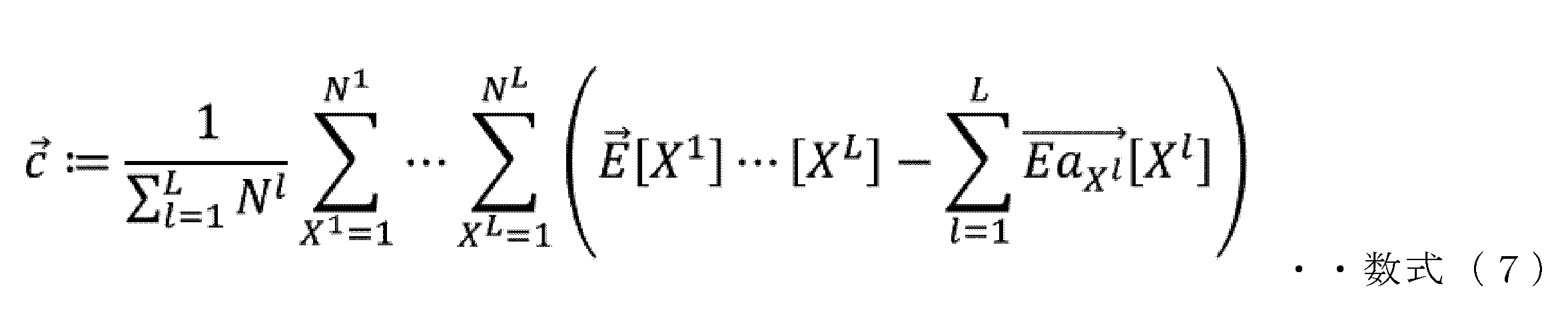
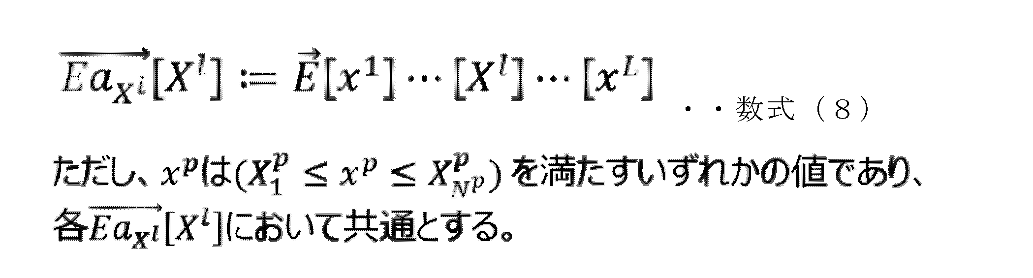

図13は、第2実施形態に係るデータ符号化装置2の構成を示す図である。図13に示されるように、第2実施形態に係るデータ符号化装置2は、軸依存データ分割部22を備える点において第1実施形態に係るデータ符号化装置1と相違する。また、第2実施形態のモデル近似符号化部21が、軸依存データを複数に分割して生成された分割後軸依存データと、上述の一次結合モデルと、に基づいてモデル近似符号化を実行する点において、第1実施形態のモデル近似符号化部11と相違する。これら相違点以外の構成については、第1実施形態と共通である。
図16は、第3実施形態に係るデータ符号化装置3の構成を示す図である。図16に示されるように、第3実施形態に係るデータ符号化装置3は、軸依存データ分割部32の構成が第2実施形態の軸依存データ分割部22と相違する点において、第2実施形態と相違する。この相違点以外の構成については、第2実施形態と共通である。
図20は、第4実施形態に係るデータ符号化装置4の構成を示す図である。図20に示されるように、第4実施形態に係るデータ符号化装置4は、モデル近似符号化部41が近似誤差算出部42を備える点において、第1実施形態のモデル近似符号化部11と相違する。また、第4実施形態に係るデータ符号化装置4は近似誤差符号化部43を備える点において、第1実施形態のデータ符号化装置1と相違する。これら相違点以外の構成については、第1実施形態と共通である。

図22は、第5実施形態に係るデータ符号化装置5の構成を示す図である。図22に示されるように、第5実施形態に係るデータ符号化装置5は、所定トレランス以上の近似誤差除去部53をさらに備える点において、第4実施形態のデータ符号化装置4と相違する。また、近似誤差符号化部54が所定トレランス以内の近似誤差量を符号化する点において、第4実施形態の近似誤差符号化部43と相違する。これら相違点以外の構成については、第4実施形態と共通である。
図25は、第6実施形態に係るデータ符号化装置6の構成を示す図である。図25に示されるように、本実施形態に係るデータ符号化装置6は、モデル近似符号化後データ符号化部62をさらに備える点において第1実施形態に係るデータ符号化装置1と相違する。この相違点以外は、第1実施形態と共通の構成である。
図26は、第7実施形態に係るデータ符号化装置7の構成を示す図である。図26に示されるように、本実施形態に係るデータ符号化装置7は、動的計画法の代わりに機械学習装置9による強化学習結果を取得する学習結果取得部を備え、該学習結果を利用して軸依存データを区間分割する点において、第3実施形態に係るデータ符号化装置3と相違する。この相違点以外の構成については、第3実施形態と共通である。

9 機械学習装置
11,21,31,41,51,61 モデル近似符号化部
22,32 軸依存データ分割部
33 動的計画法処理部
34 モデル近似符号化後の最適性評価部(最適性評価部)
35 軸依存データの部分分割部(部分分割部)
36 部分的軸依存データの最適化結果結合部(最適化結果結合部)
42 近似誤差算出部
43 近似誤差符号化部
52 近似誤差算出部
53 所定トレランスを超える近似誤差除去部(近似誤差除去部)
54 近似誤差符号化部
62 モデル近似符号化後データ符号化部(符号化後データ符号化部)
Claims (8)
- データを符号化するデータ符号化装置であって、
産業機械の各軸の座標値に依存する軸依存データの一部と、前記軸依存データを前記産業機械の各軸データの一次結合として近似する一次結合モデルと、に基づいて、前記軸依存データを符号化した符号化後軸依存データを生成するモデル近似符号化部を備える、データ符号化装置。 - 前記軸依存データを分割して複数の分割後軸依存データを生成する軸依存データ分割部をさらに備え、
前記モデル近似符号化部は、前記複数の分割後軸依存データと、前記一次結合モデルと、に基づいて、前記符号化後軸依存データを生成する、請求項1に記載のデータ符号化装置。 - 前記軸依存データ分割部は、動的計画法を実行することにより最適な前記分割後軸依存データを生成する動的計画法処理部を備え、
前記動的計画法処理部は、
前記符号化後軸依存データの最適性を評価する最適性評価部と、
前記軸依存データを複数の部分に分割して部分的軸依存データを生成する部分分割部と、
前記部分的軸依存データを拡張して結合することにより最適な前記分割後軸依存データを生成する最適化結果結合部と、を備える、請求項2に記載のデータ符号化装置。 - 前記軸依存データ分割部は、機械学習装置による強化学習結果に基づいて最適な前記分割後軸依存データを生成する、請求項2に記載のデータ符号化装置。
- 前記モデル近似符号化部は、近似誤差量を算出する近似誤差算出部を備え、
前記データ符号化装置は、前記近似誤差量を符号化して符号化後近似誤差量を生成する近似誤差符号化部をさらに備える、請求項1から4いずれかに記載のデータ符号化装置。 - 前記データ符号化装置は、前記近似誤差量から前記所定トレランスを超える近似誤差量を除去することにより、前記所定トレランス以内の近似誤差量を生成する近似誤差除去部をさらに備え、
前記近似誤差符号化部は、前記所定トレランス以内の近似誤差量を符号化して前記符号化後近似誤差量を生成する、請求項5に記載のデータ符号化装置。 - 前記データ符号化装置は、前記符号化後軸依存データを符号化する符号化後データ符号化部をさらに備える、請求項1から6いずれかに記載のデータ符号化装置。
- データを符号化するデータ符号化プログラムであって、
産業機械の各軸の座標値に依存する軸依存データの一部と、前記軸依存データを前記産業機械の各軸データの一次結合として近似する一次結合モデルと、に基づいて、前記軸依存データを符号化した符号化後軸依存データを生成させるステップをコンピュータに実行させるためのデータ符号化プログラム。
Priority Applications (5)
| Application Number | Priority Date | Filing Date | Title |
|---|---|---|---|
| CN202280097156.9A CN119404159A (zh) | 2022-06-24 | 2022-06-24 | 数据编码装置以及数据编码程序 |
| PCT/JP2022/025415 WO2023248481A1 (ja) | 2022-06-24 | 2022-06-24 | データ符号化装置及びデータ符号化プログラム |
| JP2024528258A JP7807543B2 (ja) | 2022-06-24 | 2022-06-24 | データ符号化装置及びデータ符号化プログラム |
| DE112022007089.7T DE112022007089T5 (de) | 2022-06-24 | 2022-06-24 | Datencodiervorrichtung und Datencodierprogramm |
| US18/872,020 US20250355417A1 (en) | 2022-06-24 | 2022-06-24 | Data encoding device and non-transitory computer-readable medium storing a data encoding program |
Applications Claiming Priority (1)
| Application Number | Priority Date | Filing Date | Title |
|---|---|---|---|
| PCT/JP2022/025415 WO2023248481A1 (ja) | 2022-06-24 | 2022-06-24 | データ符号化装置及びデータ符号化プログラム |
Publications (1)
| Publication Number | Publication Date |
|---|---|
| WO2023248481A1 true WO2023248481A1 (ja) | 2023-12-28 |
Family
ID=89379361
Family Applications (1)
| Application Number | Title | Priority Date | Filing Date |
|---|---|---|---|
| PCT/JP2022/025415 Ceased WO2023248481A1 (ja) | 2022-06-24 | 2022-06-24 | データ符号化装置及びデータ符号化プログラム |
Country Status (5)
| Country | Link |
|---|---|
| US (1) | US20250355417A1 (ja) |
| JP (1) | JP7807543B2 (ja) |
| CN (1) | CN119404159A (ja) |
| DE (1) | DE112022007089T5 (ja) |
| WO (1) | WO2023248481A1 (ja) |
Cited By (1)
| Publication number | Priority date | Publication date | Assignee | Title |
|---|---|---|---|---|
| CN118838292A (zh) * | 2024-09-20 | 2024-10-25 | 武汉优力克自动化系统工程股份有限公司 | 一种汽车生产线数据管理方法及系统 |
Citations (6)
| Publication number | Priority date | Publication date | Assignee | Title |
|---|---|---|---|---|
| JPH08339216A (ja) * | 1995-06-09 | 1996-12-24 | Mitsubishi Electric Corp | コンピュータ制御型数値制御装置のパラメータ設定方法およびコンピュータ制御型数値制御装置 |
| JP2000099123A (ja) * | 1998-09-22 | 2000-04-07 | Matsushita Electric Ind Co Ltd | 産業用ロボット |
| JP2011209897A (ja) * | 2010-03-29 | 2011-10-20 | Fanuc Ltd | 5軸加工機を制御する数値制御装置 |
| JP2014113674A (ja) * | 2012-12-12 | 2014-06-26 | Hirokiko Co Ltd | 補正プログラム及びその記憶媒体 |
| CN112558547A (zh) * | 2021-02-19 | 2021-03-26 | 成都飞机工业(集团)有限责任公司 | 一种五轴数控机床平动轴几何误差补偿数据快速优化方法 |
| JP2021092954A (ja) * | 2019-12-10 | 2021-06-17 | ファナック株式会社 | ワークモデルの修正量を学習する機械学習装置、制御装置、加工システム、及び機械学習方法 |
-
2022
- 2022-06-24 DE DE112022007089.7T patent/DE112022007089T5/de active Pending
- 2022-06-24 CN CN202280097156.9A patent/CN119404159A/zh active Pending
- 2022-06-24 US US18/872,020 patent/US20250355417A1/en active Pending
- 2022-06-24 JP JP2024528258A patent/JP7807543B2/ja active Active
- 2022-06-24 WO PCT/JP2022/025415 patent/WO2023248481A1/ja not_active Ceased
Patent Citations (6)
| Publication number | Priority date | Publication date | Assignee | Title |
|---|---|---|---|---|
| JPH08339216A (ja) * | 1995-06-09 | 1996-12-24 | Mitsubishi Electric Corp | コンピュータ制御型数値制御装置のパラメータ設定方法およびコンピュータ制御型数値制御装置 |
| JP2000099123A (ja) * | 1998-09-22 | 2000-04-07 | Matsushita Electric Ind Co Ltd | 産業用ロボット |
| JP2011209897A (ja) * | 2010-03-29 | 2011-10-20 | Fanuc Ltd | 5軸加工機を制御する数値制御装置 |
| JP2014113674A (ja) * | 2012-12-12 | 2014-06-26 | Hirokiko Co Ltd | 補正プログラム及びその記憶媒体 |
| JP2021092954A (ja) * | 2019-12-10 | 2021-06-17 | ファナック株式会社 | ワークモデルの修正量を学習する機械学習装置、制御装置、加工システム、及び機械学習方法 |
| CN112558547A (zh) * | 2021-02-19 | 2021-03-26 | 成都飞机工业(集团)有限责任公司 | 一种五轴数控机床平动轴几何误差补偿数据快速优化方法 |
Non-Patent Citations (1)
| Title |
|---|
| MNIH VOLODYMYR; KAVUKCUOGLU KORAY; SILVER DAVID; RUSU ANDREI A.; VENESS JOEL; BELLEMARE MARC G.; GRAVES ALEX; RIEDMILLER MARTIN; F: "Human-level control through deep reinforcement learning", NATURE, vol. 518, no. 7540, 25 February 2015 (2015-02-25), pages 529 - 533, XP037437579, DOI: 10.1038/nature14236 * |
Cited By (1)
| Publication number | Priority date | Publication date | Assignee | Title |
|---|---|---|---|---|
| CN118838292A (zh) * | 2024-09-20 | 2024-10-25 | 武汉优力克自动化系统工程股份有限公司 | 一种汽车生产线数据管理方法及系统 |
Also Published As
| Publication number | Publication date |
|---|---|
| DE112022007089T5 (de) | 2025-05-28 |
| CN119404159A (zh) | 2025-02-07 |
| JP7807543B2 (ja) | 2026-01-27 |
| JPWO2023248481A1 (ja) | 2023-12-28 |
| US20250355417A1 (en) | 2025-11-20 |
Similar Documents
| Publication | Publication Date | Title |
|---|---|---|
| CN101925925A (zh) | 基于预测的图像处理 | |
| CN116414094B (zh) | 一种焊接装配智能调度方法及系统 | |
| JP4210056B2 (ja) | 工具経路の作成装置及び方法 | |
| US20230088537A1 (en) | Generative design shape optimization based on a target part reliability for computer aided design and manufacturing | |
| JP6569497B2 (ja) | 予測装置、方法及びプログラム | |
| WO2009017583A1 (en) | Product developing method and system | |
| CN106157339A (zh) | 基于低秩顶点轨迹子空间提取的动画网格序列压缩算法 | |
| WO2022063542A1 (en) | Method and system for providing recommendations concerning a configuration process | |
| WO2023248481A1 (ja) | データ符号化装置及びデータ符号化プログラム | |
| Renaud et al. | Sequential global approximation in non-hierarchic system decomposition and optimization | |
| US20250308167A1 (en) | Mesh refinement | |
| EP0822516B1 (en) | Shape data compression method and apparatus | |
| Jolgaf et al. | Development of a CAD/CAM system for the closed-die forging process | |
| JP7807544B2 (ja) | データ復号化装置、誤差補正システム及びデータ復号化プログラム | |
| JP7410365B2 (ja) | 部材配置システム及び部材配置プログラム | |
| CN112958313A (zh) | 使用距离矩阵加权特征的智能区域补偿喷漆参数控制方法 | |
| WO2023248483A1 (ja) | 近似誤差検出装置及び近似誤差検出プログラム | |
| CN120802832A (zh) | 基于区域划分热图像的机床主轴热误差预测方法及系统 | |
| CN119537955A (zh) | 海工胶凝材料的耐久性评估方法、模型的训练方法及装置 | |
| JP4546755B2 (ja) | 解析モデルの作成支援装置 | |
| CN116802573B (zh) | 加工程序修正装置、加工程序修正方法及加工系统 | |
| CN117010666A (zh) | 一种汽修工具生产工作站智能管理方法及系统 | |
| JP2022045615A (ja) | 演算装置及び演算方法 | |
| US20250308051A1 (en) | System and method for vision measurement of object information based on deep learning | |
| CN118780011B (zh) | 一种变收缩率塑料螺旋伞齿的参数确定方法 |
Legal Events
| Date | Code | Title | Description |
|---|---|---|---|
| 121 | Ep: the epo has been informed by wipo that ep was designated in this application |
Ref document number: 22948040 Country of ref document: EP Kind code of ref document: A1 |
|
| WWE | Wipo information: entry into national phase |
Ref document number: 18872020 Country of ref document: US |
|
| WWE | Wipo information: entry into national phase |
Ref document number: 2024528258 Country of ref document: JP |
|
| WWE | Wipo information: entry into national phase |
Ref document number: 202280097156.9 Country of ref document: CN |
|
| WWE | Wipo information: entry into national phase |
Ref document number: 112022007089 Country of ref document: DE |
|
| WWP | Wipo information: published in national office |
Ref document number: 202280097156.9 Country of ref document: CN |
|
| WWP | Wipo information: published in national office |
Ref document number: 112022007089 Country of ref document: DE |
|
| 122 | Ep: pct application non-entry in european phase |
Ref document number: 22948040 Country of ref document: EP Kind code of ref document: A1 |
|
| WWP | Wipo information: published in national office |
Ref document number: 18872020 Country of ref document: US |