WO2020054087A1 - シミュレーション方法、物理量計算プログラム及び物理量計算装置 - Google Patents
シミュレーション方法、物理量計算プログラム及び物理量計算装置 Download PDFInfo
- Publication number
- WO2020054087A1 WO2020054087A1 PCT/JP2018/043836 JP2018043836W WO2020054087A1 WO 2020054087 A1 WO2020054087 A1 WO 2020054087A1 JP 2018043836 W JP2018043836 W JP 2018043836W WO 2020054087 A1 WO2020054087 A1 WO 2020054087A1
- Authority
- WO
- WIPO (PCT)
- Prior art keywords
- area
- divided
- region
- regions
- calculation
- Prior art date
- Legal status (The legal status is an assumption and is not a legal conclusion. Google has not performed a legal analysis and makes no representation as to the accuracy of the status listed.)
- Ceased
Links
Images

















Classifications
-
- G—PHYSICS
- G06—COMPUTING OR CALCULATING; COUNTING
- G06F—ELECTRIC DIGITAL DATA PROCESSING
- G06F30/00—Computer-aided design [CAD]
- G06F30/10—Geometric CAD
- G06F30/15—Vehicle, aircraft or watercraft design
-
- G—PHYSICS
- G06—COMPUTING OR CALCULATING; COUNTING
- G06F—ELECTRIC DIGITAL DATA PROCESSING
- G06F30/00—Computer-aided design [CAD]
- G06F30/20—Design optimisation, verification or simulation
- G06F30/23—Design optimisation, verification or simulation using finite element methods [FEM] or finite difference methods [FDM]
-
- G—PHYSICS
- G06—COMPUTING OR CALCULATING; COUNTING
- G06F—ELECTRIC DIGITAL DATA PROCESSING
- G06F2111/00—Details relating to CAD techniques
- G06F2111/10—Numerical modelling
-
- G—PHYSICS
- G06—COMPUTING OR CALCULATING; COUNTING
- G06F—ELECTRIC DIGITAL DATA PROCESSING
- G06F2113/00—Details relating to the application field
- G06F2113/28—Fuselage, exterior or interior
-
- G—PHYSICS
- G06—COMPUTING OR CALCULATING; COUNTING
- G06F—ELECTRIC DIGITAL DATA PROCESSING
- G06F2119/00—Details relating to the type or aim of the analysis or the optimisation
- G06F2119/08—Thermal analysis or thermal optimisation
Definitions
- the present invention relates to a simulation method, a physical quantity calculation program, and a physical quantity calculation device.
- a finite element method for example, a finite element method, a finite volume method, a voxel method, and a particle method are known as numerical analysis methods for obtaining a flow velocity distribution, a stress distribution, a temperature distribution, and the like by numerical analysis.
- Patent Document 1 a method of numerical analysis in Patent Document 1 has been proposed.
- the method of Patent Literature 1 does not require a mesh which is indispensable for a conventional numerical analysis method.
- the method of Patent Document 1 can numerically analyze a physical phenomenon while satisfying the conservation law of physical quantity in the physical phenomenon to be analyzed. Further, the method of Patent Document 1 can reduce the work and time required for generating a calculation data model while obtaining sufficient analysis accuracy.
- the problem to be solved by the present invention is to provide a technique capable of reducing the time required for solver processing in numerical analysis for numerically analyzing a physical phenomenon.
- One embodiment of the present invention is a simulation method for numerically analyzing a physical quantity in a physical phenomenon by a computer, wherein the computer divides an analysis region into a plurality of divided regions, and coordinates (Vertex) of vertices of the divided regions. And a volume of each of the divided regions based on a governing equation in the discretized divided regions derived based on the weighted residual integration method using only the amount that does not require the connectivity information (Connectivity) of the vertices. And a divided region characteristic amount indicating the characteristic of the adjacent divided regions for calculation in the divided region having the coordinates (Vertex) of the vertices of the divided region and the connectivity information (Connectivity) of the vertices as unnecessary amounts.
- a data model is generated, and a plurality of the divided areas are aggregated to generate a required number of aggregated areas.
- the coordinates (Vertex) of the vertices of the aggregated area and the vertices are generated.
- the volume adjacent to each set area is A calculation data model in the set area is generated that has a set area characteristic quantity indicating the property of the set areas as an amount that does not require the coordinates (Vertex) of the vertices of the set area and the connectivity information (Connectivity) of the vertices.
- a physical quantity that is an analysis result in the aggregate area is calculated based on a physical property value in the analysis area and a calculation data model in the aggregate area.
- One aspect of the present invention is to cause a computer to divide an analysis region into a plurality of divided regions, and use only an amount that does not require the coordinates (Vertex) of the vertices of the divided regions and the connectivity information (Connectivity) of the vertices.
- the division of a volume of each of the divided regions and a divided region characteristic amount indicating characteristics of adjacent divided regions is performed. This is required by generating a calculation data model in the divided region having the coordinates (Vertex) of the vertices of the region and the connectivity information (Connectivity) of the vertices as unnecessary amounts, and by grouping a plurality of the divided regions.
- the volume of each set area and the set area characteristic quantity indicating the characteristics of the adjacent set areas are represented by the coordinates (Vertex) of the vertex of the set area.
- generating a calculation data model in the set area having an amount that does not require the connection information (Connectivity) of the vertex based on the physical property values in the analysis area and the calculation data model in the set area. And calculating a physical quantity which is an analysis result in the set area.
- One embodiment of the present invention is a physical quantity calculation device that numerically analyzes a physical quantity in a physical phenomenon, and divides an analysis region into a plurality of divided regions and collects the plurality of divided regions to obtain a required number. And a discrete unit derived by the weighted residual integration method using only the coordinates that do not require the coordinates (Vertex) of the vertices of the divided region and the connectivity information (Connectivity) of the vertices. Derived by the weighted residual integration method using only the governing equations in the segmented divided region, the coordinates (Vertex) of the vertices of the set region, and the quantities that do not require the connectivity information (Connectivity) of the vertices.
- a storage unit for storing a governing equation in the discretized set region, and the calculation unit, based on the governing equation in the divided region stored in the storage unit, the volume of each of the divided regions and the neighboring A calculation data model in the divided region having a divided region characteristic amount indicating characteristics of the divided regions that match each other as an amount that does not require the coordinates (Vertex) of the vertex of the divided region and the connectivity information (Connectivity) of the vertex.
- a calculation data model in the set area having coordinates (Vertex) and connectivity information (Connectivity) of the vertices as unnecessary quantities is generated, and physical property values in the analysis area and calculation data in the set area are generated.
- a physical quantity calculation device which calculates a physical quantity that is an analysis result in the set area based on a model.
- the present invention provides a technique capable of reducing the time required for solver processing in numerical analysis for numerically analyzing a physical phenomenon.
- FIG. 6 is a diagram illustrating an example of a process of generating a set area in the numerical analysis method according to the embodiment.
- FIG. 6 is a diagram illustrating an example of a process of generating a set area in the numerical analysis method according to the embodiment.
- FIG. 6 is a diagram illustrating an example of a process of generating a set area in the numerical analysis method according to the embodiment.
- FIG. 6 is a diagram illustrating an example of a process of generating a set area in the numerical analysis method according to the embodiment.
- FIG. 6 is a diagram illustrating an example of a process of generating a set area in the numerical analysis method according to the embodiment.
- FIG. 7 is a diagram illustrating an example of a boundary surface characteristic amount of an aggregate region in the numerical analysis method according to the present embodiment.
- FIG. 7 is a diagram illustrating an example of a boundary surface characteristic amount of an aggregate region in the numerical analysis method according to the present embodiment.
- FIG. 7 is a diagram for describing an example of a boundary surface characteristic amount of an aggregate region at a boundary of an analysis region in the numerical analysis method according to the present embodiment.
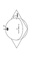
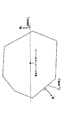
- FIG. 7 is a diagram for describing an example of a boundary surface characteristic amount of an aggregate region at a boundary of an analysis region in the numerical analysis method according to the present embodiment. It is a schematic diagram which shows the infinitely wide projection plane which has the unit normal vector of arbitrary directions which passes through the control point of a division area.
- FIG. 9 is a schematic diagram illustrating conditions that satisfy the conservation rule of physical quantity when considering a control volume of a divided region of a sphere. It is a schematic diagram which shows the infinitely wide projection plane which has the unit normal vector of arbitrary directions which passes through the control point of an aggregation area. It is a schematic diagram explaining the conditions which satisfy
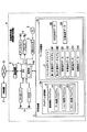
- FIG. 2 is a block diagram schematically illustrating a hardware configuration of a numerical analysis device according to the present embodiment.
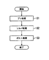
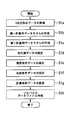
- 5 is a flowchart illustrating a numerical analysis method according to the embodiment.
- 5 is a flowchart illustrating pre-processing performed by the numerical analysis method according to the embodiment.
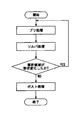
- 5 is a flowchart illustrating a solver process performed by the numerical analysis method according to the embodiment.
- 5 is a flowchart illustrating a numerical analysis method according to the present embodiment when the analysis area includes a moving boundary. It is a figure showing an example of a thermal fluid simulation result in a division field of this embodiment. It is a figure showing an example of a thermal fluid simulation result in a division field of this embodiment.
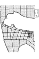
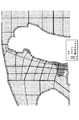
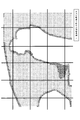
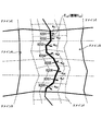
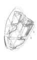
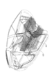
- thermofluid simulation in a collective field of this embodiment It is a figure showing an example of the generation result of the collective field (domain 6) of the thermal fluid simulation of this embodiment. It is a figure showing an example of a result (air temperature) of a thermofluid simulation in a collective field of this embodiment. It is a figure showing an example of a result (flow velocity vector) of a thermofluid simulation in a collective field of this embodiment. It is a figure showing an example of a result (air temperature) of a thermofluid simulation in a collective field of this embodiment. It is a figure showing an example of a result (flow velocity vector) of a thermofluid simulation in a collective field of this embodiment.
- thermofluid simulation in a collective field of this embodiment It is a figure showing an example of a result (air temperature) of a thermofluid simulation in a collective field of this embodiment. It is a figure showing an example of a result (flow velocity vector) of a thermofluid simulation in a collective field of this embodiment. It is a figure showing an example of a result (air temperature) of a thermofluid simulation in a collective field of this embodiment. It is a figure showing an example of a result (flow velocity vector) of a thermofluid simulation in a collective field of this embodiment.
- ⁇ The“ physical phenomenon ”in the present embodiment means a phenomenon that can be reproduced by simulation.
- a simulation related to the cabin of an automobile solar radiation from the sun passing through the window glass, heat taken from the outer surface of the window glass according to the vehicle speed, air blowing by air conditioning, heat convection in the cabin, heat radiation, etc. Heat transfer phenomenon.
- ⁇ The“ physical quantity ”in the present embodiment means a temperature, a heat flux, a stress, a pressure, a flow velocity, and other values, which are analysis results of a simulation of a physical phenomenon.
- the “analysis region” in the present embodiment means a target region of an analysis model set for simulating a physical phenomenon.
- the analysis area is a cabin space surrounded by an object such as an automobile body and window glass.
- the calculation load in the solver processing is reduced by increasing the size of the divided area.
- Increasing the size of the divided area means reducing the number of divisions of the analysis area. Therefore, if the size of the divided area is increased, the calculation load in the solver processing is reduced. Therefore, it can be said that the calculation load in the solver process is reduced by reducing the number of divisions of the analysis region. However, if the number of divisions is reduced, the analysis accuracy will deteriorate.
- the number of divisions of the analysis region is reduced to reduce the calculation load in the solver process, and the deterioration of analysis accuracy due to the decrease in the number of divisions of the analysis region is reduced. It is compatible with suppression.
- a calculation is performed on a division region characterized by an amount that does not require Vertex (vertex coordinates of the division region) and Connectivity (connection information).
- a data model for the first time hereinafter referred to as a “first calculation data model”.
- a data model for calculation hereinafter, referred to as a “second calculation data model” in a set area in which a plurality of the divided areas are set is generated.
- Aggregate regions are also characterized by quantities that do not require Vertex and Connectivity.
- the divided area for generating the aggregated area is characterized by an amount that does not require Vertex and Connectivity, so that the calculation load in the solver processing is reduced as described later.
- the calculation load in the solver processing is reduced by reducing the number of divided analysis areas. And the suppression of the deterioration of the analysis accuracy due to the reduction in the number of divisions of the analysis region can be achieved, and the analysis can be performed at a higher speed.
- the discretization governing equation used in the present embodiment is expressed in a format including coordinates (Vertex), which is a quantity defining the geometrical shape of the divided area, and connectivity information (Connectivity) of the vertex, as in the related art. However, it does not require coordinates (Vertex), which is an amount defining the geometric shape of the divided area, and connectivity information (Connectivity) of the vertex. In the present embodiment, the coordinates (Vertex), which is an amount defining the geometric shape, and the connection information (Connectivity) of the vertex are hereinafter simply referred to as “an amount defining the geometric shape”. Furthermore, the discretized governing equation used in the present embodiment does not require an amount that defines the geometric shape of a set area obtained by collecting a plurality of divided areas.
- the discretized governing equation used in the present embodiment can be obtained by intentionally stopping in the process of deriving the equation using the amount defining the conventional geometric shape based on the weighted residual integration method. it can.
- the discretization governing equation used in the present embodiment is represented by an amount that does not require the geometrical shape of the divided region and the aggregated region. For example, it depends only on the two of the volume of the divided region and the characteristic amount of the boundary surface.
- the format can be
- the discretization governing equation used in the present embodiment can be in a form that depends only on two of the volume of the aggregated region and the boundary surface characteristic amount.
- the object to be analyzed is divided into minute regions as a premise, and the discretized governing equation is assumed to be used on the assumption that the amount that defines the geometric shape of the minute region is used. Is being derived.
- the discretization governing equation used in the present embodiment is derived based on an idea different from these conventional methods.
- the present embodiment is characterized by using a discretized governing equation derived based on this idea, and does not depend on the quantity defining the geometric shape, unlike the conventional numerical analysis method. Further, the present embodiment has various remarkable effects such as a reduction in calculation time by enabling calculation in an aggregate area that aggregates divided areas, which is not disclosed or suggested in Patent Literature 1.
- the amount that does not require the amount defining the geometric shape is an amount that can be defined without using Vertex and Connectivity.
- the volume of a divided region when considering the volume of a divided region, there are a plurality of geometrical shapes of the divided region so that the volume of the divided region has a predetermined value. That is, the geometrical shape of the divided region whose volume takes a predetermined value may be a cube or a sphere. Then, for example, the volume of the divided area is proportional to the cube of the average distance to the adjacent divided area, for example, under the constraint that the sum of all the divided areas is equal to the volume of the entire analysis area. It can be defined by an optimization calculation as follows. Therefore, the volume of the divided region can be regarded as an amount that does not require a specific geometric shape of the divided region.
- volume of the divided region can be regarded as an amount that does not require an amount that defines a specific geometric shape of the aggregate area.
- the boundary surface characteristic amount of the divided region for example, the area of the boundary surface, the normal vector of the boundary surface, the perimeter of the boundary surface, and the like can be considered. There are a plurality of geometrical shapes of the divided area to become the values. Then, for example, the boundary surface characteristic amount of the divided region is calculated based on the boundary surface method under the constraint that the length of the area-weighted average vector of the normal vector is zero with respect to all the boundary surfaces surrounding each divided region. The direction of the line vector is made closer to the line segment connecting the control points (see FIG. 1) of the two adjacent divided areas, and the sum of all the boundary surface areas surrounding the divided areas is the cube of the volume of the divided area.
- the boundary surface characteristic amount of the divided region can be regarded as an amount that does not require an amount that defines a specific geometric shape of the divided region.
- Such a feature related to the boundary surface characteristic amount of the divided region similarly exists for the boundary surface characteristic amount of the aggregate region. Therefore, the boundary surface characteristic amount of the aggregated region can be regarded as an amount that does not require an amount defining a specific geometric shape of the aggregated region.
- the control points in the collective area are referred to as collective control points.
- the ⁇ discrete governing equation using only the amount that does not require the amount defining the geometric shape '' is a discrete value in which the value to be substituted is only the amount that does not require the vertex and connectivity. Means the governing equation.
- the volume of the aggregated region and the boundary surface characteristic amount of the aggregated region are used as amounts that do not require the amount defining the geometric shape. For this reason, the calculation data model created in the pre-processing does not have Vertex and Connectivity, but has the volume of the aggregated region, the boundary surface characteristic amount of the aggregated region, and other auxiliary data (for example, the aggregated region described later). And the coordinates of the set control point).
- the physical quantity in each area is determined based on the volume of the set area, which is an amount that does not require the quantity defining the geometric shape, and the boundary surface characteristic amount. Can be calculated. For this reason, it is possible to calculate the physical quantity without giving the second calculation data model an amount that defines the geometric shape of the aggregate area. Therefore, by using this embodiment, in the pre-processing, a second calculation data model having at least the volume of the aggregation region and the boundary surface characteristic amount (the area of the boundary surface and the normal vector of the boundary surface) is created. As a result, the physical quantity can be calculated without creating a calculation data model having a quantity defining the geometric shape.
- the second calculation data model having no amount defining the geometric shape does not require the amount defining the geometric shape of the aggregation region, it is bound to the amount defining the geometric shape of the aggregation region. It can be created without.
- the second calculation data model having no amount defining the geometric shape can be created much more easily than the calculation data model having the amount defining the geometric shape. Therefore, according to the present embodiment, the work load in creating the calculation data model can be reduced.
- an amount defining the geometric shape may be used. That is, the volume of the divided region, the boundary surface characteristic value, and the like may be calculated using the amount defining the geometric shape in the pre-processing. Even in such a case, in the solver processing, the physical quantity can be calculated if there is a volume of the aggregated area or the boundary surface characteristic value. Also, there is no restriction on the geometrical shape of the set area, for example, no restriction due to distortion or torsion of the divided area, and the work load in creating the calculation data model can be reduced.
- the present embodiment in the pre-processing, there is no restriction on the geometric shape of the aggregated region, so that the aggregated region can be changed to an arbitrary shape. For this reason, it is possible to easily fit the analysis region to the region to be actually analyzed without increasing the number of aggregation regions, and it is possible to improve the analysis accuracy without increasing the calculation load.
- the distribution density of the aggregation region can be arbitrarily changed, so that the analysis accuracy can be further improved while allowing the calculation load to increase within a necessary range.
- the information for associating the divided areas for exchanging the physical quantity includes connection information (link) between the adjacent divided areas and the distance between the adjacent divided areas.
- the divided areas associated by the link need not necessarily be spatially adjacent to each other, and may be spatially separated. Such a link is not related to the quantity defining the geometric shape, and can be created in a very short time when compared to the quantity defining the geometric shape.
- the coordinates of the control points arranged inside the divided area may be provided in the first calculation data model as needed.
- a required number of set areas is generated by collecting a plurality of divided areas.
- a second calculation data model having information for associating the aggregate regions for exchanging the volume of the aggregate region, the boundary surface characteristic amount (the area of the boundary surface, the normal vector of the boundary surface) and the physical quantity is created.
- the information for associating the set areas for exchanging the physical quantities and the link information (link) between the adjacent set areas also have the same features as the features for the divided areas.
- the coordinates of the control points arranged inside the aggregation area may be provided in the second calculation data model as needed.
- the first calculation data model of the divided region having the volume of the divided region, the boundary surface characteristic amount, the link, the coordinates of the control point, and the like, and the boundary condition and the initial condition are solved.
- a physical quantity is calculated by solving a discretized governing equation using the volume of the divided region, the boundary surface characteristic quantity, and the like included in the received first calculation data model.
- the second calculation data model having the volume of the set area, the boundary surface characteristic amount, the link, the coordinates of the control point, and the like, and the boundary conditions, the initial conditions, and the like are subjected to the solver processing. hand over.
- the solver processing a physical quantity is calculated by solving a discretized governing equation using the volume of the set area, the boundary surface characteristic quantity, and the like included in the received second calculation data model.
- the point that the physical quantity is calculated without using the quantity defining the geometric shape in the solver processing is greatly different from the conventional finite volume method, and this point is a great feature of the present embodiment. is there.
- Such features are obtained by using a discretized governing equation that uses only quantities that do not require quantities that define the geometric shape in the solver process.
- the calculation data model can be created much more easily than in the conventional finite volume method, and the work load in creating the calculation data model can be reduced.
- the numerical analysis method using the present embodiment has a process of dividing an analysis region into a plurality of divided regions (hereinafter, referred to as a “process of dividing into a plurality of divided regions”). Further, this numerical analysis method uses only the coordinates that do not require the coordinates (Vertex) of the vertices of the divided area and the connectivity information (Connectivity) of the vertices, and also uses the discretization derived based on the weighted residual integration method. Based on the governing equations for the divided regions, the coordinates of the vertices of the divided regions (Vertex) and the connection information (Connectivity) of the vertices are calculated based on the volume of each divided region and the divided region characteristic amount indicating the characteristics of the adjacent divided regions. (Hereinafter, referred to as “process for generating a first calculation data model in a divided area”).
- the numerical analysis method has a process of generating a required number of aggregate regions by grouping a plurality of divided regions (hereinafter, referred to as “process of generating aggregate regions”). Furthermore, the present numerical analysis method uses only the coordinates that do not require the coordinates (Vertex) of the vertices of the set area and the connectivity information (Connectivity) of the vertices, and also uses the discretization derived based on the weighted residual integration method. Based on the governing equation for the set area, the coordinates of the set area vertex (Vertex) and the connection information (Connectivity) of the set area are calculated based on the volume of each set area and the set area characteristic amount indicating the characteristics of the adjacent set areas.
- the numerical analysis method has a process of calculating a physical quantity based on a physical property value in the analysis area and a calculation data model in the aggregation area.
- a process of dividing the analysis region for creating the first calculation data model into a plurality of divided regions will be described.
- the analysis region is finely divided by cells that do not use the amount defining the geometric shape.
- cell R 1, R 2, R 3 ⁇ are divided regions obtained by dividing the analysis region, each having a volume V a, V b, the V c ⁇ ⁇ ⁇ .
- the boundary surface E is a surface replacement of physical quantity is performed between the cell R 1 and the cell R 2, corresponding to the boundary surface in the present embodiment.
- the area Sab indicates the area of the boundary surface E, and is one of the boundary surface characteristic amounts in the present embodiment.
- [N] ab indicates a normal vector of the boundary surface E, and is one of the boundary surface characteristic amounts in the present embodiment.
- control point a, b, c ⁇ ⁇ ⁇ are arranged inside each cell R 1, R 2, R 3, each cell R 1 in FIG. 1, R 2, R 3 ⁇ of It is located at the center of gravity.
- the control points a, b, c... Do not always need to be arranged at the positions of the centers of gravity of the cells R 1 , R 2 , R 3 .
- ⁇ indicates the distance from the control point a to the boundary E when the distance from the control point a to the control point b is 1, and the boundary E is a line segment connecting the control point a and the control point b. Is a ratio indicating at which subdivision point of the subscript exists. Note that the distance from the control point a to the control point b is an example of the distance between adjacent divided regions.
- the interface is not limited only between the cell R 1 and the cell R 2, exists between all adjacent cells. Then, the normal vector of the boundary surface and the area of the boundary surface are also given for each boundary surface.
- the first calculation data model in the actual divided area includes the arrangement data of the control points a, b, c,... And the cells R 1 , in which the control points a, b, c,. R 2, R 3 ⁇ volume V a, V b, and volume data indicative of the V c ⁇ ⁇ ⁇ , and the area data indicating the area of each boundary surface, the normal vector (hereinafter "normal of the boundary surface Vector ").
- the area of the boundary surface which is the boundary characteristic amount indicating the characteristics of the boundary surface between the cells R 1 , R 2 , R 3, ..., And the boundary surface between the adjacent cells R 1 , R 2 , R 3 ,.
- the normal vector of the boundary surface which is the characteristic amount of the boundary surface that indicates the characteristic of.
- Each cell R 1 , R 2 , R 3 ... Has control points a, b, c. Therefore, the volumes V a , V b , V c ... Of the cells R 1 , R 2 , R 3 ... Are virtually occupied by control points a, b, c. Can be regarded as the volume of
- the first calculation data model of the present numerical analysis method may use, as necessary, ratio data indicating a ratio ⁇ indicating which subdivision point of the line segment connecting the control points sandwiching the boundary surface exists. Have.
- the flow velocity at each control point is determined as the flow velocity at each cell.
- the present numerical analysis method uses the Navier-Stokes equation shown by the following equation (1) and the continuous equation shown by the following equation (2) in the case of fluid analysis.
- Expression (1) is expressed as Expression (3) below.
- Equation (2) is expressed as the following equation (4).
- V indicates the volume of the control volume
- ⁇ VdV indicates the integral with respect to the volume V
- S indicates the area of the control volume
- ⁇ SdS indicates the integral with respect to the area S
- [n] represents the normal vector of S
- ⁇ / ⁇ n indicates the normal derivative.
- the density ⁇ and the viscosity coefficient ⁇ of the fluid are constants.
- the following constantization can be extended to the case where the physical property value of the fluid changes with time, space, temperature, and the like.
- Niab is a component of [n] ab .
- m is the number of all control points that have a connection relationship (a relationship sandwiching the boundary surface) with the control point a.
- equation (5) dividing the (6) V a (volume control volume control point a)
- equation (6) is the following formula It is shown as (8).
- Expression (7) is expressed as Expression (10) below, and Expression (8) is expressed as Expression (11) below.
- [u] ab, u iab , P ab, ( ⁇ u i / ⁇ n) ab is an amount independent of the amount that defines the geometry of the boundary surface E.
- ⁇ ab defined by the equation (9) is also an amount (area / volume), which is irrelevant to the amount defining the geometric shape of the control volume.
- equations (10) and (11) can be used to calculate the physical quantity using only the quantity that does not require the quantity that defines the geometric shape that defines the cell shape. Is an arithmetic expression based on
- the above-mentioned first calculation data model is created prior to the physical quantity calculation (solver processing), and the first calculation data model and the discretized governing equations of equations (10) and (11) are calculated in the physical quantity calculation.
- the flow velocity can be calculated without using any quantity that defines the geometric shape of the control volume in the physical quantity calculation.
- the flow velocity can be calculated without using any amount defining the geometric shape in the physical quantity calculation, it is not necessary to provide the first calculation data model with the amount defining the geometric shape. . Therefore, when creating the first calculation data model, it is not necessary to be restricted by the geometric shape of the cell, and the shape of the cell can be set arbitrarily. For this reason, according to the present numerical analysis method, as described above, the restriction on the correction work of the three-dimensional shape data can be greatly eased.
- the physical quantity ⁇ ab can also be obtained by the following equation (13) by using the ratio ⁇ of which of the line segments connecting the control points sandwiching the boundary surface is present at the internally dividing point.
- the first calculation data model has the ratio data indicating the ratio ⁇
- the physical quantity on the boundary surface E is separated from the control point a and the control point b using Expression (13). It can be calculated using a weighted average according to the distance.
- the equation of the continuum model includes the first-order partial derivative (partial derivative) as shown in equation (1).
- the derivative of the equation of the continuum model is converted into the area using the partial integral, the Gaussian divergence theorem, or the generalized Green's theorem, and the order of the derivative is reduced.
- the first derivative can be made the zero-order derivative (scalar quantity or vector quantity).
- the first derivative term of the equation of the continuum model is treated as a scalar quantity or vector quantity on the boundary surface by converting the area integral from the volume integral. These values can be interpolated from the physical quantities on each control point by the above-described linear interpolation or the like.
- the partial derivative of the second order may be included.
- ⁇ / ⁇ n indicates the normal direction derivative
- ⁇ / ⁇ n ab indicates the [n] ab direction derivative
- the second derivative term of the equation of the continuum model is converted into a normal direction derivative of the physical quantity ⁇ (normal of S ab [n] ab in the ab direction), The form is obtained by multiplying the components niab and njab .
- the vector [r] ab between the control points a and b is obtained from the position vector [r] a of the control point a and the position vector [r] b of the control point b as shown in the following equation (18). Is defined as
- Equation (14) all linear partial differential equations are represented as linear sums of constants and terms obtained by multiplying first, second, and other partial derivatives by coefficients.
- Equation (15) to (19) when the physical quantity ⁇ is replaced by the first-order partial derivative of ⁇ , the volume integral of the higher-order partial derivative is converted to the lower-order partial derivative as in Equation (14). Can be determined by the area of.
- this procedure is sequentially repeated from a low-order partial differential, partial derivatives of all terms constituting the linear partial differential equation are calculated by the physical quantity ⁇ of the control point and the equation (12) or the equation (13).
- [psi ab is [psi on the boundary surface, the components of the normal vector of the control points the distance between which is determined from a control point between the vectors defined by equation (18), the area S ab of the boundary surface E, the boundary surface E n All can be obtained from iab and njab .
- this numerical analysis method does not require a quantity that defines a geometric shape in calculating a physical quantity. For this reason, when creating the first calculation data model, if the volume of the control volume, the area of the boundary surface, and the normal vector are obtained without using the quantities that define the geometric shape, the expression (10) is obtained. Using the discretized governing equation of equation (11), the flow velocity can be calculated without using any cell geometry, which is the geometry of the control volume.
- the volume of the control volume it is not always necessary to obtain the volume of the control volume, the area of the boundary surface, and the normal vector without using the specific geometric shape of the control volume.
- the conventional finite element method is used even if the specific geometric shape of the control volume, specifically, Vertex and Connectivity is used. Since there is no restriction on the divided region, such as the finite volume method, that is, there is no restriction on the distortion and twist of the divided region, the calculation data model can be easily created as described above.
- the geometric shape is derived from various equations (mass conservation equation, momentum conservation equation, energy conservation equation, advection diffusion equation, wave equation, etc.) based on the weighted residual integration method.
- Any discretionary governing equation that can calculate a physical quantity using only an amount that does not require a prescribed amount can be used in the present numerical analysis method.
- control volumes (cells) automatically generated in the analysis area are collected, and a newly set control volume is defined as a domain.
- the domain is a control volume and is a set sum of cells.
- a new domain may be set by collecting the set domains.
- a set sum of a plurality of domains is set.
- domains are indicated by thin lines.
- a new domain is set by grouping a plurality of domains.
- the newly set domain is indicated by a bold line.
- a newly set domain is also a control volume, and is a set sum of domains.
- the volume of the newly set domain and the coordinate vector of the control point of the newly set domain are calculated by Expressions (20) and (21). As shown in FIG. 6, control points are shown. Then, the newly set domain is handled in the same manner as the domain.
- the domain created by the union of the set of cells be domain 1
- the domain created by the union of the set of domain 1 be domain 2
- the domain created by the union of the set of domain 2 be domain 3.
- the domain can be set to a domain 1, domain 2, domain 3,...
- the domain can be set to a domain 1, domain 2, domain 3,..., Final domain, and a hierarchical structure type from the control volume (cell).
- the final domain may be set from domain 1 without going through domain 2 or domain 3.
- the domain is set in a hierarchical structure with the domain 1, domain 2, domain 3,..., The final domain from the control volume (cell), or the final domain is set from the domain 1 without passing through the domain 2. In this case, the cell division accuracy of the boundary shape of the first analysis region is not lost.
- the finite volume method is limited to an icosahedron, and the finite element method cannot define an intra-element interpolation function of a polyhedron exceeding 6 hexahedrons.
- the present embodiment is conceived from the point that there is no motivation or suggestion to form the aggregated area from the divided areas, and it has a remarkable effect which is impossible with the conventional method.
- the automatically generated control volume (cell) enables numerical analysis while satisfying the physical quantity conservation rules such as mass balance (mass conservation), momentum conservation, and energy conservation between cells. Therefore, even from the control volume (cell), domains 1, 2, 3,..., And the final domain are set in a hierarchical structure type. Even when the domain and the hierarchical structure are set, the conservation law of the physical quantity between the domains is satisfied.
- the analysis region is roughly divided into orthogonal lattice regions, and cells including the coordinates of the control points are collected in the orthogonal lattice.
- ⁇ ⁇ ⁇ ⁇ As shown in FIG. 8, set a domain control point in the analysis area. From the control points of the domain, cells including the coordinates of the control points are collected in a sphere having a radius specified in advance. The radius is gradually increased, and all cells in the analysis area are gathered in one of the domains.
- a voxel may be generated in a region including the analysis region by the voxel method, and the voxel may be used as a domain. In this case, cells including the coordinates of the control point are collected in the voxel.
- control volumes (cells) automatically generated in the analysis area When a domain is newly set by assembling control volumes (cells) automatically generated in the analysis area according to the control volume (cell) aggregation method, the cell division accuracy of the boundary shape of the first analysis area is set. Is not lost. Therefore, the control volumes (cells) automatically generated in the analysis area are aggregated according to the control volume (cell) aggregation method, and the numerical values are satisfied between the newly set domains while satisfying the physical quantity conservation rule. Can be analyzed.
- FIG. 9 is a conceptual diagram illustrating an example of a boundary surface characteristic amount in a set area according to the numerical analysis method of the present invention.
- FIG. 9 shows a plurality of divided regions for dividing the analysis region and a plurality of aggregated regions.
- the domain A and the domain B surrounded by a solid line are an aggregation area.
- a figure surrounded by a broken line is a divided area.
- the cells R201 to R208 are divided areas.
- the domain A is a set area obtained by collecting a plurality of divided areas including the cells R201 to R208.
- the boundary surface E AB is a surface on which a physical quantity is exchanged between the domain A and the domain B, and corresponds to a boundary surface in the second calculation data model.
- the area S AB indicates the area of the boundary surface E AB and is one of the boundary surface characteristic amounts of the aggregate region in the present embodiment.
- Each of [n] a1 to [n] a8 is a normal vector which is an amount indicating the characteristics of the boundary surface between cells that are in contact with each other at the boundary surface E AB .
- the domain A and the domain B in FIG. 10 are the domain A and the domain B in FIG.
- the control point Ac and the control point Bc are located inside the domain A and the domain B, respectively.
- NS AB is the total number of boundary surfaces of the cell b belonging to the domain B and in contact with the boundary surface E AB
- S AB of the boundary surface between the domain A and the domain B, and the boundary between the domain A and the domain B
- S ab is the area of the boundary surface of cell b belonging to domain B and in contact with boundary surface E AB .
- FIG. 11 illustrates a case where the domain A is in contact with the boundary with the external space in the analysis area.
- the set sum of the boundary surfaces of the cells a that are in contact with the domain B is calculated, whereby the equations (22) and ( Similarly to 23), the area S AB of the boundary between the domain A and the domain B and the normal vector [n] AB of the boundary between the domain A and the domain B can be derived.
- domains are generated by assembling control volumes (cells) automatically generated in the analysis area.
- the domain A is calculated using the interface characteristic amount (the area S ab of the interface, the normal vector [n] ab of the interface) at the interface S ab between the cell a and the cell b. and with respect to the boundary surface S AB between the domain B, by calculating the set union, interface characteristic amount at the interface S AB between domain a and domain B (of the boundary surface area S AB, the interface The normal vector [n] AB ) was determined.
- the continuum numerical analysis method using cells that do not use quantities defining the geometric shape was applied to the domain as exactly the same calculation method.
- the domain can be set in a hierarchical structure type including domain 1, domain 2, domain 3, ..., the final domain. Therefore, the continuum numerical analysis method can be applied to all of the domains set to the domain 1, domain 2, domain 3,..., The final domain, and the hierarchical structure type.
- the numerical analysis using the cells of the coarse division number is an analysis.
- the result may include many errors.
- cell division on the order of tens of millions to hundreds of millions of cells or more can be performed in a short time by a computer having a relatively low-capacity memory if only cells are automatically generated.
- domain 1, domain 2, domain 3,... can be divided into domains. If the number of domain divisions is on the order of thousands to tens of thousands, numerical analysis can be performed in a short time by a computer having a relatively low-capacity memory.
- the boundary shape of the domain in which the cells are aggregated is very complicated and multifaceted, but by using a numerical analysis method of the continuum using cells that does not use the quantity defining the geometric shape, the boundary of the analysis region is obtained.
- the numerical analysis of the continuum can be executed in a short time with a computer having a relatively low memory while suppressing errors included in the analysis result to a degree that does not cause a problem, while maintaining the cell division accuracy of the shape.
- equations (3) and (4) are derived.
- V indicates the volume of the set region
- ⁇ VdV indicates the integral related to the volume V of the set region
- S indicates the integral of the set region.
- ⁇ SdS indicates integration with respect to the boundary surface S of the set region
- [n] indicates a normal vector of the boundary surface S of the set region
- the component of the normal vector [n] of the boundary surface S is shown, and ⁇ / ⁇ n is the normal direction derivative of the boundary surface S of the set area.
- the density ⁇ and the viscosity coefficient ⁇ of the fluid are constants for the sake of simplicity.
- the following constantization can be extended to the case where the physical property value of the fluid changes with time, space, temperature, and the like.
- the subscript AB stick [n] AB, [u ] AB, u iAB, n iAB, P AB, ( ⁇ u i / ⁇ n) AB , the boundary between the collection region B the set region A It indicates that it is a physical quantity on the surface E AB .
- NiAB is a component of [n] AB .
- m A is the number of all sets control points in the coupling relationship between the set region A (relation sandwiching the boundary surface).
- Expressions (24) and (25) are divided by V A (the volume of the aggregation region A), Expression (24) is expressed as Expression (26), and Expression (25) is expressed as Expression (27) Is shown as
- [u] AB , u iAB , P AB , and ( ⁇ u i / ⁇ n) AB are weighted averages of physical quantities on the set control point A and the set control point B (the advection term Is approximately determined by a weighted average in consideration of the windward property, and the positional relationship between the distance and direction between the set control points A and B and the boundary surface E AB of the set area existing therebetween (the above ratio) ⁇ ) and the direction of the normal vector of the boundary surface E AB of the set area.
- [u] AB, u iAB , P AB, ( ⁇ u i / ⁇ n) AB is an amount independent of the amount that defines the geometry of the boundary surface E AB aggregate areas.
- ⁇ AB defined by Expression (28) is also an amount (area / volume), and is an amount irrelevant to the amount defining the geometric shape of the control volume of the aggregate area.
- equations (29) and (30) are computations based on the weighted residual integration method, in which the physical quantity can be calculated using only the vertices defining the shape of the aggregation area and the quantity that does not require connectivity. It is an expression.
- the above-described second calculation data model is created prior to the physical quantity calculation (solver processing), and the calculation data model and the discretized governing equations of equations (29) and (30) are used in the physical quantity calculation.
- the flow velocity without using any quantity that defines the geometric shape of the aggregate area in the physical quantity calculation.
- the data model for the second calculation is also used in the data model for the second calculation, similarly to the data model for the first calculation. There is no need to have a quantity defining the geometric shape.
- the physical quantities on the boundary surface E AB such as [u] AB and P AB are calculated by the calculation equations (12) to (19) in the first calculation data model.
- the physical quantity ⁇ is replaced from the physical quantity of the control point of the divided area to the physical quantity of the control point of the collective area, and the area of the boundary surface of the divided area and the normal vector are calculated by the equation (22) of the boundary area of the collective area and the normal
- the position (coordinate) vector of the control point in the divided area is replaced with the position (coordinate) vector (21) of the control point in the set area in the distance (18) between the control points in the divided area.
- the area of the boundary surface of the divided region between the control points in the continuous expression (6) representing the law of conservation of mass of the divided region is controlled even when viewed from the control point a side. Assuming that they are the same even from the point b side, the mass flux ( ⁇ [n] ⁇ [u]) ⁇ S between the control points is opposite in polarity on the control point a side and the control point b side, and their absolute values are equal. Become. Therefore, when the equation (6) is summed over all the divided regions in the analysis region, the mass flux between the divided regions is deducted to zero and canceled, and the mass inflow and outflow are calculated for the entire analysis region to be calculated. It indicates that the masses to be measured are equal.
- the condition that the area of the boundary surface between the two control points of the divided region matches and the normal vector of the boundary surface of the divided region is one of A condition is required that the positive and negative signs are opposite and the absolute values match when viewed from the control point side and when viewed from the other control point side.
- the unit normal vector is a normal vector having a unit length.
- S i represents the area of the boundary surface E i
- [n] i represents the unit first normal vector of the boundary surface E i
- m represents the total number of surfaces of the control volume.
- Expression (32) indicates that the polyhedron forming the control volume forms a closed space. This equation (32) holds even when a part of the polyhedron constituting the control volume is concave.
- Green's theorem is a fundamental theorem for discretization of continuum. Therefore, in the case where the volume integral is transformed into an area and discretized according to Green's theorem, the condition that the expression (32) is satisfied is essential to satisfy the conservation law.
- first calculation conditions When performing the numerical analysis using the first calculation data model and the physical quantity calculation, the following three conditions (hereinafter referred to as “first calculation conditions”) must be satisfied in order to satisfy the conservation law of the physical quantity. ”) Is required.
- the area of the boundary surface of the collective region between the collective control points in the continuous equation (25) representing the law of conservation of mass of the collective region is viewed from the collective control point A side.
- the control point B side the mass flux between the collective control points A and the collective control point B are opposite in sign and have the same absolute value. Therefore, when the equation (25) is summed over all the collective regions in the analysis region, the mass flux between the collective regions is deducted to zero and canceled, so that the mass inflow and outflow for the entire analysis region to be calculated are calculated. It indicates that the masses to be measured are equal.
- the unit second normal vector passing through the collective control point A and having an arbitrary direction [ it is necessary condition that the following equation (35) holds when considering an infinitely large projection plane P d with N] P.
- the unit second normal vector is a second normal vector having a unit length.
- Q i is the area of one boundary surface E di of the domain
- [N] i is the unit second normal vector of the boundary surface E di
- M is the total number of surfaces of the set control volume.
- the subscript i is an integer of 1 to M.
- Equation (35) shows that the polyhedrons forming the set control volume form a closed space. This equation (35) holds even when a part of the polyhedron constituting the collective control volume is concave.
- Green's theorem is a fundamental theorem for discretization of continuum. Therefore, in the case where the volume integral is transformed into an area and discretized according to Green's theorem, the condition that the expression (35) is satisfied is necessary to satisfy the conservation law.
- second calculation conditions In performing the numerical analysis using the above-described second calculation data model and the physical quantity calculation, the following three conditions (hereinafter referred to as “second calculation conditions”) must be satisfied in order to satisfy the conservation law of the physical quantity. ”) Is required.
- the conservation rule when the conservation rule is satisfied, it is necessary to create the first and second calculation data models so as to satisfy these conditions.
- the cell shape of the divided region when creating the calculation data model, the cell shape of the divided region can be arbitrarily modified, and the aggregated region is created by summing the divided region cells. Therefore, it is possible to easily create the first and second calculation data models so as to satisfy the above three conditions.
- this numerical analysis method has a feature that the analysis accuracy does not deteriorate even if the number of divisions of the analysis region is small.
- the geometric shape is derived from various equations (mass conservation equation, momentum conservation equation, energy conservation equation, advection diffusion equation, wave equation, etc.) based on the weighted residual integration method.
- Any discretionary governing equation that can calculate a physical quantity using only an amount that does not require a prescribed amount can be used in the present numerical analysis method.
- Patent Document 1 describes that a discretized governing equation can be derived for a case where an analysis region is divided by a divided region. However, a case where an analysis region is divided by a set region is similarly discretized. A governing equation can be derived.
- FIG. 17 is a block diagram schematically showing a hardware configuration of the numerical analysis device A of the present embodiment.
- the numerical analysis device A of the present embodiment is configured by a computer such as a personal computer or a workstation, and includes a CPU 1, a storage device 2, a DVD drive 3, an input device 4, an output device 5, and a communication device. 6 is provided.
- the CPU 1 is electrically connected to the storage device 2, the DVD drive 3, the input device 4, the output device 5, and the communication device 6, processes signals input from these various devices, and outputs a processing result. I do.
- the CPU 1 is a specific example of the operation unit 1op.
- the storage device 2 includes an internal storage device such as a memory and an external storage device such as a hard disk drive.
- the storage device 2 stores information input from the CPU 1 and outputs the stored information based on a command input from the CPU 1. .
- the storage device 2 includes a program storage unit 2a and a data storage unit 2b.
- the program storage unit 2a stores a numerical analysis program P.
- the numerical analysis program P is an application program that is executed in a predetermined OS (Operating System), and causes the numerical analysis apparatus A including a computer to function to perform numerical analysis. Then, the arithmetic unit 1op executes the numerical analysis program P, whereby each function of the numerical analysis device A of the present embodiment is realized.
- OS Operating System
- the numerical analysis program P has a pre-processing program P1, a solver processing program P2, and a post-processing program P3.
- the preprocessing program P1 causes the numerical analysis device A of the present embodiment to execute preprocessing (preprocessing) for executing a solver process, and uses the numerical analysis device A of the present embodiment as a first calculation data model creation unit. By having it function, a first calculation data model is created. Further, the pre-processing program P1 causes the numerical analysis device A of the present embodiment to function as a second calculation data model creation unit to create a second calculation data model. Further, the pre-processing program P1 causes the numerical analysis device A of the present embodiment to execute setting of conditions necessary for executing the solver processing, and furthermore, a solver that summarizes the calculation data model and the set conditions. The input data file F is created.
- the preprocessing program P1 causes the numerical analysis device A of the present embodiment to function as a first calculation data model creation unit, and after the first calculation data model is created, executes the numerical analysis device A of the present embodiment. Function as a second calculation data model creation unit.
- the preprocessing program P1 causes the numerical analysis device A of the present embodiment to function as the first calculation data model creation unit and the second calculation data model creation unit, the preprocessing program P1 Then, three-dimensional shape data including the cabin space of the vehicle is obtained, and an analysis region indicating the cabin space of the vehicle included in the obtained three-dimensional shape data is created.
- the discretized governing equation described in the numerical analysis method using the above-described embodiment is used.
- the discretized governing equations described in the numerical analysis method using the present embodiment are, specifically, using only the quantities that do not require the quantities that define the geometric shape and using the weighted residual integration This is a discretized governing equation derived based on the method. For this reason, when creating the first calculation data model and the second calculation data model, the shape of the divided region, the shape of the aggregated region based on the divided region, and the shape of the analysis region are arbitrarily changed under conditions that satisfy the conservation rule. it can. Therefore, a simple operation of correcting or changing the cabin space of the vehicle included in the three-dimensional shape data is sufficient.
- the pre-processing program P1 instructs the numerical analysis device A of the present embodiment to add a small closed curved surface to a hole or a gap existing in the cabin space of the automobile included in the acquired three-dimensional shape data.
- a repairing process is performed by a wrapping process that covers the device.
- the pre-processing program P1 forms the divided area on the numerical analysis device A of the present embodiment as described in the processing of dividing into the plurality of divided areas, and performs the entire cabin space repaired by the lapping process or the like. Execute the creation of the analysis area including the area. Subsequently, the pre-processing program P1 cuts an area that protrudes from the cabin space among the divided areas created for the numerical analysis device A of the present embodiment, thereby creating an analysis area indicating the cabin space. Let it run. Also in this case, since the above-described discretized governing equation is used in the solver process, a region that protrudes from the cabin space in the analysis region can be easily cut.
- the boundary with the external space does not become stair-like, and experience and the formation of an analysis region near the boundary of the external space such as the cut cell method of the voxel method have It does not require special modifications or processes involving a very large amount of manual work requiring trial and error. Therefore, in the present embodiment, there is no problem related to the processing of the boundary with the external space, which is a problem in the voxel method.
- the analysis region is configured by a divided region that does not depend only on the orthogonal lattice shape by filling a gap between the cabin space and the cut region with a new divided region of an arbitrary shape as described later.
- the analysis region is filled with the divided region without overlapping.
- the preprocessing program P1 when the preprocessing program P1 causes the numerical analysis device A of the present embodiment to function as a first calculation data model generation unit, the preprocessing program P1 converts the cabin space generated by the numerical analysis device A of the present embodiment into a cabin space. A process of virtually arranging one control point in each of the divided regions included in the analysis region shown is executed, and the arrangement information of the control points and the volume data of the control volume occupied by each control point are stored. .
- the preprocessing program P1 provides the numerical analysis device A according to the present embodiment with a boundary surface between the divided regions. The calculation of the area of the boundary surface and the first normal vector is executed, and the area of the boundary surface and the first normal vector are stored.
- the preprocessing program P1 creates control volume or control point connection information (link) and stores the link. Let it.
- the pre-processing program P1 sends, to the numerical analysis apparatus A of the present embodiment, the volume of the control volume occupied by each control point, the area of the boundary surface, the first normal vector, and the arrangement information of the divided area.
- the arrangement information of the control points to be represented and the link are combined to create a first calculation data model.
- the arrangement indicated by the arrangement information may be indicated using, for example, coordinates.
- the preprocessing program P1 When the preprocessing program P1 causes the numerical analysis device A of the present embodiment to function as a second calculation data model generation unit, the preprocessing program P1 generates a first calculation data model for the numerical analysis device A of this embodiment. Is used to collect control volumes (cells) by the method shown in FIG. 7 or FIG. 8, and an aggregate area is generated in the analysis area indicating the cabin space.
- the preprocessing program P1 when the preprocessing program P1 causes the numerical analysis device A of the present embodiment to function as a second calculation data model generation unit, the preprocessing program P1 converts the cabin space generated by the numerical analysis device A of the present embodiment into a cabin space.
- the process of virtually arranging one set control point inside each set area included in the analysis area shown is executed, the set control point arrangement information, and the volume of the domain in which each set control point is set Store the data.
- the pre-processing program P1 indicates a place where each set control point is arranged by causing the numerical analysis device A of the present embodiment to execute the set control point calculation processing in the processing of virtually arranging the set control points. Get information.
- the numerical analysis apparatus A of the present embodiment acquires the volume of the control volume and the arrangement information of the control points included in the first calculation data model, and calculates the equations (20) and (21). Is performed to calculate the arrangement location of the set control point.
- the preprocessing program P1 provides the numerical analysis device A of the present embodiment with a boundary surface between the set regions. (Hereinafter referred to as “set area boundary surface characteristic amount calculation process”), and the area of these boundary surfaces and the second normal vector are stored.
- the numerical analysis apparatus A of the present embodiment acquires information on the area of the boundary surface included in the first calculation data model and the first normal vector, and calculates the expression (22) and the expression This is a process of calculating the area of the boundary surface between the set regions and the second normal vector by executing the calculation of (23).
- the preprocessing program P1 creates connection information (link) of a domain or a set control point, and stores the link. Let it.
- the pre-processing program P1 sends, to the numerical analysis apparatus A of the present embodiment, the volume of the domain in which each of the set control points is arranged, the area of the boundary surface, the second normal vector, and the arrangement of the set area.
- the arrangement information of the set control points representing the information and the link are combined to create a second calculation data model.
- the arrangement indicated by the arrangement information may be indicated using, for example, coordinates.
- the preprocessing program P1 causes the numerical analysis device A of the present embodiment to set conditions necessary for executing the above-described solver processing, the physical property setting, the boundary condition setting, and the initial setting are performed. Set conditions and calculation conditions.
- the physical property values are air density, viscosity coefficient and the like in the cabin space.
- the boundary condition is a condition that defines a law of exchange of physical quantities between control points.
- the boundary condition includes information indicating a set area facing a boundary surface between the cabin space and the external space.
- the initial condition indicates an initial physical quantity at the time of executing the solver process, and is an initial value of the flow velocity in each of the divided region and the aggregated region.
- the calculation condition is a condition for calculation in the solver process, for example, the number of iterations or a convergence criterion.
- the pre-processing program P1 causes the numerical analysis device A of the present embodiment to form a GUI (Graphical User Interface). More specifically, the pre-processing program P1 displays a graphic on the display 5a of the output device 5 and makes it operable by the keyboard 4a and the mouse 4b of the input device 4.
- GUI Graphic User Interface
- the solver processing program P2 causes the numerical analysis device A of the present embodiment to execute a solver process, and causes the numerical analysis device A of the present embodiment to function as a physical quantity calculation device.
- the solver processing program P2 causes the solver input data file F to numerically calculate the physical quantity in the analysis area.
- the solver processing program P2 provides the numerical analysis device A of the present embodiment with the Navier-Stokes data included in the solver input data file F.
- the generation of the discretization coefficient matrix of the expression and the continuous expression is performed, and the generation of the data table for forming the matrix is performed.
- the solver processing program P2 provides the numerical analysis device A of the present embodiment with the Navier-Stokes equation (29) described above. From the discretized governing equation based on the above equation and the discretized governing equation based on the continuous equation shown in the above equation (30), a large-scale sparse matrix equation for matrix calculation shown in the following equation (37) is assembled. Let it.
- the solver processing program P2 performs not only the numerical calculation using the second calculation data model created from the set area as an input but also the numerical calculation using the first calculation data model created from the divided area as an input. You can also.
- a discretized governing equation based on the Navier-Stokes equation shown in the above-described equation (10) and a continuous equation shown in the above-described equation (11) From the discretized governing equation based on the following formula (37), a large-scale sparse matrix equation for matrix calculation is set up.
- [A] indicates a large-scale sparse matrix
- [B] indicates a boundary condition vector
- [X] indicates a solution of flow velocity
- the solver processing program P2 instructs the numerical analysis device A of the present embodiment to assemble the incidental conditions into a matrix equation. Let it run.
- the solver processing program P2 calculates the solution of the matrix equation by the CG method (conjugate gradient method) or the like and updates the solution using the following equation (38) for the numerical analysis device A of the present embodiment. , A convergence condition is determined, and a final calculation result is obtained.
- CG method conjuggate gradient method
- the post-processing program P3 causes the numerical analysis device A of the present embodiment to execute post-processing, and causes the numerical analysis device A of the present embodiment to execute a process based on the calculation result obtained in the solver process. .
- the post-processing program P3 causes the numerical analysis device A of the present embodiment to execute a calculation result visualization process and an extraction process.
- the visualization process is a process of causing the output device 5 to output, for example, cross-sectional contour display, vector display, isosurface display, and animation display.
- the extraction processing is to extract a quantitative value of an area designated by an operator and output the numerical value or a graph to the output device 5 as a numerical value or a graph, or to extract a quantitative value of an area designated by an operator and output a file. Is executed.
- the post-processing program P3 causes the numerical analysis device A of the present embodiment to execute automatic report creation, display and analysis of calculation residuals.
- the data storage unit 2b stores the first calculation data model M1, the second calculation data model M2, the boundary condition data D1 indicating the boundary condition, the calculation condition data D2 indicating the calculation condition, and the physical property values. It stores a solver input data file F having physical property value data D3 and initial condition data D4 indicating initial conditions, three-dimensional shape data D5, calculation result data D6, and the like. Further, the data storage unit 2b temporarily stores intermediate data generated during the processing of the CPU 1.
- the DVD drive 3 is configured to take in the DVD medium X, and outputs data stored in the DVD medium X based on a command input from the CPU 1.
- the numerical analysis program P is stored in the DVD medium X, and the DVD drive 3 outputs the numerical analysis program P stored in the DVD medium X based on a command input from the CPU 1. I do.
- the input device 4 is a man-machine interface between the numerical analysis device A of the present embodiment and an operator, and includes a keyboard 4a and a mouse 4b as pointing devices.
- the output device 5 visualizes and outputs a signal input from the CPU 1, and includes a display 5a and a printer 5b.
- the communication device 6 exchanges data between the numerical analysis device A of the present embodiment and an external device such as a CAD device C, and is electrically connected to a network B such as an in-house LAN (Local Area Network). ing.
- a network B such as an in-house LAN (Local Area Network).
- the numerical analysis method includes a pre-process (step S1), a solver process (step S2), and a post process (step S3).
- the CPU 1 Prior to performing the numerical analysis method of the present embodiment, the CPU 1 takes out the numerical analysis program P stored in the DVD medium X loaded in the DVD drive 3 from the DVD medium X, and stores the program in the program storage unit of the storage device 2. 2a.
- the CPU 1 executes the numerical analysis based on the numerical analysis program P stored in the storage device 2. More specifically, the CPU 1 executes pre-processing (step S1) based on the pre-processing program P1 stored in the program storage unit 2a, and performs solver processing based on the solver processing program P2 stored in the program storage unit 2a. (Step S2) is executed, and post processing (Step S3) is executed based on the post processing program P3 stored in the program storage unit 2a.
- the CPU 1 executes the pre-processing (step S1) based on the pre-processing program P1, whereby the numerical analysis device A of the present embodiment functions as a calculation data model creation unit.
- the CPU 1 executes the solver process (step S2) based on the solver process program P2, so that the numerical analysis device A of the present embodiment functions as a physical quantity calculation unit.
- FIG. 19 is a flowchart showing the pre-processing (step S1).
- the CPU 1 when the pre-processing (step S1) is started, the CPU 1 causes the communication device 6 to acquire the three-dimensional shape data D5 including the cabin space of the vehicle from the CAD device C via the network B. (Step S1a).
- the CPU 1 stores the acquired three-dimensional shape data D5 in the data storage unit 2b of the storage device 2.
- the CPU 1 creates a first calculation data model based on the three-dimensional shape data D5 acquired in step S1a (step S1b).
- the CPU 1 virtually arranges one control point in each divided area included in the analysis area indicating the cabin space.
- the CPU 1 calculates the center of gravity of the divided area, and virtually arranges one control point for each center of gravity. Then, the CPU 1 calculates the arrangement information of the control points, the volume of the control volume occupied by each control point (the volume of the divided area in which the control points are arranged), and temporarily stores the data in the data storage unit 2b of the storage device 2. .
- the CPU 1 calculates the area of the boundary surface that is the boundary surface between the divided areas and the first normal vector, and temporarily stores the area of the boundary surface and the first normal vector in the data storage unit 2b of the storage device 2. To memorize it.
- the CPU 1 creates a link between the divided areas, and temporarily stores the link between the divided areas in the data storage unit 2b of the storage device 2.
- the CPU 1 creates a database of the control point arrangement information, the volume of the control volume occupied by each control point, the area and the normal vector of the boundary surface, and the link stored in the data storage unit 2b.
- a first calculation data model is created, and the created first calculation data model is stored in the data storage unit 2b of the storage device 2.
- step S1b a configuration is adopted in which a divided area is formed first, control points are arranged thereafter, and the volume of the divided area in which the apparatus is arranged is allocated to each control point.
- control points in the analysis area first, and assign a volume to each control point later.
- weighting is performed on each control point based on the radius up to collision with a different control point and the distance to a control point in a connected relationship (associated with a link).
- the CPU 1 forms a GUI, and receives a command (for example, a command indicating the density of the divided area or a command indicating the shape of the divided area) from the GUI.
- a command for example, a command indicating the density of the divided area or a command indicating the shape of the divided area
- the operator can arbitrarily adjust the arrangement of the control points and the shape of the divided area by operating the GUI.
- the CPU 1 compares the command input from the GUI with the three conditions for satisfying the conservation rule stored in the numerical analysis program, and displays the fact on the display 5a if the condition is not satisfied. .
- the CPU 1 creates a second calculation data model based on the first calculation data model created in step S1b (step S1c).
- the CPU 1 uses the created first calculation data model to collect control volumes (cells) by the method shown in FIG. 7 or FIG. Generate Next, the CPU 1 virtually arranges one set control point in each set area included in the analysis area indicating the cabin space.
- the CPU 1 calculates the set control points by the equations (20) and (21), and virtually arranges one set control point for each set area. I do.
- the CPU 1 calculates the arrangement information of the collective control points, the volume of the collective control volume occupied by each collective control point (the volume of the collective area where the collective control points are arranged), and temporarily stores the information in the data storage unit 2b of the storage device 2. To memorize it.
- the CPU 1 calculates the area of the boundary surface, which is the boundary surface between the collective regions, and the second normal vector, and temporarily stores the area of the boundary surface and the second normal vector in the data storage unit 2b of the storage device 2. To memorize it.
- the CPU 1 creates a link of the set area, and temporarily stores the link of the set area in the data storage unit 2b of the storage device 2.
- the CPU 1 stores the arrangement information of the set control points, the volume of the set area having each set control point, the area of the boundary surface, the second normal vector, and the link stored in the data storage unit 2b in a database. Then, a second calculation data model is created, and the created second calculation data model is stored in the data storage unit 2b of the storage device 2.
- the CPU 1 forms a GUI, and receives a command (for example, a command indicating the density of the divided area or a command indicating the shape of the divided area) from the GUI.
- a command for example, a command indicating the density of the divided area or a command indicating the shape of the divided area
- the operator can arbitrarily adjust the arrangement of the set control points and the shape of the set area by operating the GUI.
- the set area is a set of control volumes (cells)
- the shape cannot be changed by ignoring the control volume (cell) in the set area.
- the CPU 1 compares the command input from the GUI with the three conditions for satisfying the conservation rule stored in the numerical analysis program, and displays the fact on the display 5a if the condition is not satisfied. .
- the CPU 1 sets physical property value data (step S1d). Specifically, the CPU 1 displays a physical property value input screen on the display 5a using the GUI, and outputs a signal indicating the physical property value input from the keyboard 4a or the mouse 4b as the physical property data D3 to the data storage unit 2b.
- the physical property value is set by temporarily storing the value in the.
- the physical property value is a characteristic value of air as a fluid in the cabin space, such as a density of air, a viscosity coefficient, and the like.
- the CPU 1 sets boundary condition data (step S1e). Specifically, the CPU 1 displays an input screen of the boundary condition on the display 5a using the GUI, and uses a signal indicating the boundary condition input from the keyboard 4a or the mouse 4b as the boundary condition data D1 in the data storage unit 2b.
- the boundary condition data is set by temporarily storing the data.
- the boundary conditions referred to here are the discretized governing equations governing the physical phenomena of the cabin space, the specific information of the set control points facing the interface between the cabin space and the external space, and the relationship between the cabin space and the external space. The conditions for heat transfer between the elements are shown.
- the numerical analysis method of the present embodiment aims to obtain the flow velocity in the cabin space by numerical analysis, the discretization governing equation based on the Navier-Stokes equation (29) is used as the discretization governing equation. And a discretized governing equation (30) based on the equation of continuity.
- these discretized governing equations are, for example, a plurality of discretized governing equations stored in the numerical analysis program P in advance by the operator from the plurality of discretized governing equations displayed on the display 5a. Is selected by using.
- the CPU 1 sets initial condition data (step S1f). Specifically, the CPU 1 displays an initial condition input screen on the display 5a using the GUI, and uses a signal indicating the initial condition input from the keyboard 4a or the mouse 4b as the initial condition data D4 as the data storage unit 2b. , The initial condition data is set.
- the initial conditions referred to here are an initial flow velocity at each control point (each divided area) and an initial flow velocity at each set control point (each set area).
- the CPU 1 sets calculation condition data (step S1g). Specifically, the CPU 1 displays a calculation condition input screen on the display 5a using the GUI, and outputs a signal indicating the calculation condition input from the keyboard 4a or the mouse 4b as the calculation condition data D2 in the data storage unit 2b.
- the calculation condition data is set by temporarily storing the calculation condition data.
- the calculation conditions here are the conditions for the calculation in the solver process (step S2), and indicate, for example, the number of iterations and the convergence criterion.
- step S1h the CPU 1 creates a solver input data file F (step S1h).
- the CPU 1 calculates the first calculation data model M1 created in step S1b, the second calculation data model M2 created in step S1c, and the physical property value data D3 set in step S1d.
- the boundary condition data D1 set in step S1e, the initial condition data D4 set in step S1f, and the calculation condition data D2 set in step S1g are stored in the solver input data file F, so that solver input is performed.
- step S1 When the pre-processing (step S1) as described above is completed, the CPU 1 executes the solver processing (step S2) shown in the flowchart of FIG. 18 based on the solver processing program P2.
- step S2a when the solver process (step S2) is started, the CPU 1 acquires the solver input data file F created in the pre-process (step S1) (step S2a).
- the solver input data is already stored in the data storage unit 2b. Since the file F is stored, step S2a can be omitted.
- the pre-process (step S1) and the solver process (step S2) are executed by different devices, it is necessary to acquire the solver input data file F carried by the network or the removable disk. S2a needs to be performed.
- the solver input data refers to data stored in the solver input data file F, and includes a first calculation data model M1, a second calculation data model M2, boundary condition data D1, calculation condition data D2, and property value data. D3 and initial condition data D4.
- the CPU 1 determines the consistency of the solver input data by analyzing whether all the solver input data capable of executing the physical quantity calculation in the solver processing is stored in the solver input data file F.
- the CPU 1 displays an error on the display 5a (step S2b +), and further displays a screen for inputting the data of the inconsistent portion. . Thereafter, the CPU 1 adjusts the solver input data based on the signal input from the GUI (Step S2c), and executes Step S2a again.
- step S2e the CPU 1 executes an initial calculation process
- the CPU 1 performs an initial calculation process by creating a discretized coefficient matrix from the discretized governing equations stored in the boundary condition data D1, and further creating a data table for matrix calculation.
- the discretized governing equations stored in the boundary condition data D1 are, for example, a discretized governing equation (29) based on the Navier-Stokes equation and a discretized governing equation (30) based on the continuous equation.
- the CPU 1 When performing the numerical calculation using the first calculation data model created from the divided area as the solver input data, the CPU 1 creates a discretized coefficient matrix from the discretized governing equation stored in the boundary condition data D1. Then, an initial calculation process is performed by creating a data table for matrix calculation.
- the discretized governing equations stored in the boundary condition data D1 are, for example, a discretized governing equation (10) based on the Navier-Stokes equation and a discretized governing equation (11) based on the continuous equation.
- the CPU 1 sets up a large-scale sparse matrix equation (step S2f). Specifically, the CPU 1 obtains a large-size matrix for the matrix calculation represented by the aforementioned equation (37) from the discretized governing equation (29) based on the Navier-Stokes equation and the discretized governing equation (30) based on the continuous equation. Build up a large-scale sparse matrix equation.
- the CPU 1 calculates the discretized governing equation (10) based on the Navier-Stokes equation and the continuous equation.
- a large-scale sparse matrix equation for matrix calculation represented by the above equation (37) is assembled from the discretized governing equation (11) based on the equation.
- the CPU 1 determines whether or not there are incidental conditions such as incompressibility and contact in the discretized governing equation. These incidental conditions are stored in the solver input data file F as boundary condition data, for example.
- the CPU 1 determines that an incidental condition exists in the discretized governing equation, the CPU 1 executes the incorporation of the large-scale matrix equation of the incidental condition (step S2h), and then executes the calculation of the large-scale matrix equation (step S2i). I do. On the other hand, if the CPU 1 determines that there is no incidental condition in the discretized governing equation, the CPU 1 performs the calculation of the large-scale matrix equation (step S2i) without executing the incorporation of the incidental condition large-scale matrix equation (step S2h). Execute.
- the CPU 1 solves the large-scale matrix equation by, for example, the CG method (conjugate gradient method), and updates the solution using the above-described equation (38) (step S2j).
- the CG method conjuggate gradient method
- the CPU 1 determines whether or not the residual of the equation (38) has reached the convergence condition (step S2k). Specifically, the CPU 1 calculates the residual of the equation (38), compares the residual with the convergence condition included in the calculation condition data D2, and thereby determines whether the residual of the equation (38) has reached the convergence condition. Is determined.
- the CPU 1 updates the physical property values and then executes step S2g again. That is, the CPU 1 repeats steps S2f to S2k while updating the physical property values until the residual of the equation (38) reaches the convergence condition.
- the CPU 1 obtains a calculation result (step S21). Specifically, the CPU 1 obtains a calculation result by storing the solution of the physical quantity calculated in the immediately preceding step S2i as calculation result data in the data storage unit 2b.
- step S2 the flow velocity of the air in the cabin space is obtained.
- step S2 corresponds to the physical quantity calculation method of the present embodiment.
- step S3 When the above-described solver processing (step S2) is completed, the CPU 1 executes post processing (step S3) based on the post processing program P3.
- the CPU 1 generates, for example, section contour data, vector data, iso-surface data, and animation data from the calculation result data based on a command input from the GUI, and outputs the data to the output device 5. To visualize.
- the CPU 1 extracts a quantitative value (calculation result) in a part of the cabin space into a numerical value or a graph based on a command input from the GUI, and makes the output device 5 visualize the numerical value or the graph. Output numerical values and graphs as a file. Further, based on a command input from the GUI, the CPU 1 generates an automatic report from the calculation result data, displays and analyzes the calculation residual, and outputs the result.
- the numerical analysis method, and the numerical analysis program of the present embodiment changes the three-dimensional shape data according to the result of the post-processing and repeats the processing of the flowchart of FIG. 18 again. Also, the calculation of the physical quantity can be performed within a realistic time.
- the user when the user evaluates the calculation result data obtained by the post-processing and determines that the desired result has been obtained from the three-dimensional shape data to be analyzed, the user may end the simulation. In addition, if the user evaluates the calculation result data obtained by the post-processing and determines that the desired result is not obtained by the three-dimensional shape data to be analyzed, the user corrects the three-dimensional shape data. Then, the simulation may be executed again.
- the simulation shows a desired result
- the physical entity represented by the three-dimensional shape data that was the object of the analysis such as a car cabin, cockpit, house, electrical equipment or industrial equipment that constitutes a closed space
- the design of the inside of the device, or the manufacturing device of glass, steel, etc. is satisfactory, and the physical entity may be manufactured and produced.
- the simulation does not show the desired result, it is determined that the design of the physical entity represented by the three-dimensional shape data to be analyzed is not satisfactory, and the design of the physical entity is changed. The simulation is executed again based on the changed three-dimensional shape data.
- the second calculation including the volume of the set control volume, the area of the boundary surface, and the second normal vector in the pre-processing A data model M2 is created, and the physical quantity in each set control volume is calculated by the solver process using the volume of the set control volume, the area of the boundary surface, and the second normal vector included in the second calculation data model M2. Is done.
- the numerical analysis method of the present embodiment is a physical phenomenon analysis method for numerically analyzing a physical phenomenon.
- the analysis region is filled with the divided region without overlapping. Therefore, the six conditions (a1) to (c1) and (a2) to (c2) for satisfying the storage side described above are satisfied, and the flow velocity can be calculated by satisfying the conservation rule.
- the numerical analysis device A of the present embodiment configured as described above is a calculation data model that does not have a quantity that defines a geometric shape, and creates a calculation data model that satisfies the conservation law. It is possible to achieve both a reduction in the calculation load in the solver process by reducing the number of divisions of the region and a reduction in the analysis accuracy even if the number of divisions of the analysis region is reduced.
- the workload of the first and second calculation data models in the pre-processing is significantly reduced, and the solver It is possible to reduce the calculation load in the processing.
- the analysis region includes the moving boundary and the shape of the analysis region changes in time series, as shown in the flowchart of FIG.
- the numerical analysis method, and the numerical analysis program of the present embodiment changes the three-dimensional shape data according to the post-processing result and repeats the processing of the flowchart in FIG. 21 again. Also, the calculation of the physical quantity can be performed within a realistic time.
- the user when the user evaluates the calculation result data obtained by the post-processing and determines that the desired result has been obtained from the three-dimensional shape data to be analyzed, the user may end the simulation. In addition, if the user evaluates the calculation result data obtained by the post-processing and determines that the desired result is not obtained by the three-dimensional shape data to be analyzed, the user corrects the three-dimensional shape data. Then, the simulation may be executed again.
- the simulation shows a desired result
- the physical entity represented by the three-dimensional shape data that was the object of the analysis such as a car cabin, cockpit, house, electrical equipment or industrial equipment that constitutes a closed space
- the design of the inside of the device, or the manufacturing device of glass, steel, etc. is satisfactory, and the physical entity may be manufactured and produced.
- the simulation does not show the desired result, it is determined that the design of the physical entity represented by the three-dimensional shape data to be analyzed is not satisfactory, and the design of the physical entity is changed. The simulation is executed again based on the changed three-dimensional shape data.
- the moving boundary refers to the boundary of an object that changes as the target object moves in the analysis area.
- the case where the analysis region includes the moving boundary and the shape of the analysis region changes in a time series includes, for example, a case where a phenomenon from a state where no person is present in the cabin until a person enters the cabin is reproduced. In addition, for example, there is a case where a phenomenon in which a heating target moves in a heating furnace is reproduced.
- the present embodiment is not limited to this, and discrete equations derived from at least one of mass conservation equation, momentum conservation equation, angular momentum conservation equation, energy conservation equation, advection diffusion equation and wave equation
- the physical quantity can be obtained by numerical analysis using the generalization governing equation.
- the present embodiment is not limited to this, and another amount (for example, the circumference of the boundary surface) can be used as the boundary surface characteristic amount.
- the present embodiment is not limited to this, and if it is not necessary to satisfy the conservation rule, it is not necessary to create the calculation data model so as to satisfy the above six conditions.
- the present embodiment is not limited to this, and it is not always necessary to arrange control points inside the divided area.
- numerical analysis can be performed by replacing the volume of the control volume occupied by the control points with the volume of the divided area.
- the analysis area is first divided into a plurality of control volumes (cells) to create a first calculation data model, and then an aggregate area (domain) in which the control volumes (cells) are aggregated
- the analysis region was divided by the above to create a second calculation data model.
- calculation was performed using the second calculation data model.
- the second calculation data model may be a calculation data model based on a domain in which cells are aggregated, and may be a calculation data model in a new domain in which domains in which cells are aggregated are further aggregated. Is also good.
- FIGS. 22 to 38 are diagrams illustrating an example of the results of a thermal fluid simulation performed using the first calculation data model (divided region) and the second calculation data model (aggregated region) in the present embodiment.
- the numerical calculation method using the Navier-Stokes equation shown in equation (1) and the continuous equation shown in equation (2) as basic equations for fluid analysis has been described.
- the discretization rule using only the quantity that does not require the quantity defining the geometric shape is used. It has been explained that the equation can be derived.
- heat advection The diffusion equation was used as the basic equation.
- an example of the analysis area is a cabin of an automobile, and an example of a boundary condition is summer and cooling and air conditioning conditions.
- the reference temperature outside the vehicle is 35 ° C.
- the heat transfer coefficient outside the vehicle is 40 W / m 2 K
- the number of passengers is 4
- the air-conditioning blow-out wind speed is 5 m / s
- the air-conditioner blow-out temperature is 8 ° C.
- the numerical analysis device A divides the analysis area (cabin of the automobile) into cells that do not require the coordinates (Vertex) of the vertices and the connectivity information (Connectivity) of the vertices.
- FIGS. 22 to 24 show an example of the results of a 3D thermo-fluid simulation performed using the first calculation data model in which the analysis area (car cabin) is divided into about 4.5 million cells.
- FIG. 22 is a temperature contour diagram on a vertical cross section at the center of the driver's seat in the cabin space, which is an analysis area.
- FIG. 23 is a diagram showing temperature values at seven sampling points on the vertical cross section (hereinafter, temperature values). Is expressed in K (Kelvin).)
- FIG. 24 is a flow rate contour diagram on a vertical cross section at the center of the driver's seat in the cabin space, which is an analysis area, where the direction of the flow rate is indicated by the arrow and the magnitude of the flow rate is indicated by the size of the arrow.
- the results shown in FIGS. 22 to 24 required about 30 hours of calculation time using a PC equipped with a CPU @ Xeon (2.6 GHz) manufactured by Intel Corporation until obtaining the calculation results in a steady state.
- the numerical analysis device A automatically generates approximately 4.5 million cells for the analysis area (cabin of the vehicle).
- the numerical analysis apparatus A generates 27 aggregated regions (domains) from approximately 4.5 million cells shown in FIGS. 25 to 32 by the above-described process of generating aggregated regions from cells.
- An example of a result of generating each of the 27 aggregation regions is shown in FIGS.
- DCP is a control point of an aggregation area (domain)
- CCP is one of the control points of a cell.
- 25 to 30 show domains 1 to 6 in order.
- the numerical analysis apparatus A acquires the outer surface of each set area.
- the numerical analysis device A acquires a boundary condition between the acquired outer surface and a member in contact with the outer surface. Boundary conditions may vary depending on the material of the member that the outer surface contacts.
- FIGS. 31 and 32 show an example of the results of a 3D thermo-fluid simulation performed using the second calculation data model including the above-mentioned 27 aggregation regions (domains).
- FIG. 31 is a temperature contour diagram on a vertical cross section at the center of the driver's seat in the cabin space, which is an analysis area, and shows temperature values at seven sampling points on the vertical cross section.
- the temperature values at the seven sampling points in FIG. 31 are shown separately for the upper temperature value and the lower temperature value in parentheses, respectively.
- the temperature values in parentheses at the bottom are the first calculation divided into about 4.5 million divided areas (cells) shown in FIG. Values of the results of 3D thermo-fluid simulation performed using the data model for simulation. Comparing the upper and lower temperature values, although there is a difference between the temperature values of several degrees, they agree well on average.
- FIG. 32 is a temperature contour diagram on a vertical cross section at the center of the driver's seat in the cabin space, which is an analysis area, and is a diagram in which a flow velocity vector is superimposed on the same vertical cross section. It can be seen that a circulating flow is formed in the cabin space by the air-conditioning blow-out flow, but a 3D thermal-fluid simulation result performed using the first calculation data model divided into about 4.5 million cells shown in FIG. In comparison with FIG. 32, it can be seen that the detailed distribution of the flow in the cabin space cannot be calculated in FIG.
- FIGS. 33 and 34 show an example of the results of a 3D thermofluid simulation performed using the second calculation data model including 792 aggregation regions (domains).
- FIG. 33 is a temperature contour diagram on a vertical section at the center of the driver's seat in the cabin space, which is an analysis area, and shows temperature values at seven sampling points on the vertical section. As in FIG. 31, the temperature values at the seven sampling points are shown separately for the upper temperature value and the lower temperature value in parentheses, respectively, and the upper row contains 792 aggregation regions (domains). It is a temperature value of the 3D thermo-fluid simulation result performed using the data model for the second calculation, and the temperature value in the lower parenthesis is the data model for the first calculation divided into about 4.5 million cells shown in FIG. 3 shows a temperature value of a result of a 3D thermal fluid simulation performed by using. Comparing the upper and lower temperature values, although there is a difference between the temperature values of several degrees, they agree well on average.
- FIG. 34 is a temperature contour diagram on a vertical cross section at the center of the driver's seat in the cabin space, which is an analysis area, and is a diagram in which a flow velocity vector is superimposed on the same vertical cross section. It can be seen that a circulating flow is formed in the cabin space by the air-conditioning blow-out flow, but it can be seen from FIG. 34 that the detail of the flow in the cabin space is improved in comparison with FIG. 32.
- FIGS. 35 and 36 show an example of the results of a 3D thermal fluid simulation performed using the second calculation data model including 16055 aggregated regions.
- FIG. 35 is a temperature contour diagram on a vertical section at the center of the driver's seat in the cabin space, which is an analysis area, and shows temperature values at seven sampling points on the vertical section. As in FIG. 31, the temperature values at the seven sampling points are shown separately for the upper temperature value and the lower temperature value in parentheses, however, the upper value includes 16055 aggregated regions (domains). It is a temperature value of the 3D thermo-fluid simulation result performed using the data model for the second calculation, and the temperature value in the lower parenthesis is the data model for the first calculation divided into about 4.5 million cells shown in FIG. 3 shows a temperature value of a result of a 3D thermal fluid simulation performed by using. Comparing the upper and lower temperature values, the difference between the temperature values is about 1 degree, which is in very good agreement.
- FIG. 36 is a temperature contour diagram on a vertical cross section at the center of the driver's seat in the cabin space, which is an analysis area, and is a diagram in which flow velocity vectors are superimposed on the same vertical cross section. It can be seen that a circulating flow is formed by the air-conditioning blow-off flow in the cabin space, but in comparison with FIGS. 32 and 34, in FIG. 36, the degree of detail of the flow in the cabin space is greatly improved, and in the cabin space It can be seen that the local flow and vortex of have been calculated.
- FIGS. 37 and 38 show an example of the results of a 3D thermo-fluid simulation performed using the second calculation data model including 66257 aggregate regions.
- FIG. 37 is a temperature contour diagram on a vertical cross section at the center of the driver's seat in the cabin space, which is an analysis area, and shows temperature values at seven sampling points on the vertical cross section. As in FIG. 31, the temperature values at the seven sampling points are shown separately for the upper temperature value and the lower temperature value in parentheses, respectively, and the upper value includes 66257 aggregated regions (domains). Temperature values in 3D thermo-fluid simulations performed using the second calculation data model. The temperature values in parentheses at the bottom are the first calculation data model divided into about 4.5 million cells shown in FIG. 3 shows a temperature value of a result of a 3D thermal fluid simulation performed by using. When the temperature values in the upper and lower stages are compared, the difference between the temperature values is zero, which is in very good agreement.
- FIG. 38 is a temperature contour diagram on a vertical cross section at the center of the driver's seat in the cabin space, which is an analysis area, and is a diagram in which a flow velocity vector is superimposed on the same vertical cross section. It can be seen that a circulating flow is formed in the cabin space by the air-conditioning blow-off flow, but in comparison with FIGS. 32 and 34, in FIG. 38, the degree of detail of the flow in the cabin space is greatly improved, and in the cabin space The local flow and vortex of can also be calculated. Compared with the 3D thermo-fluid simulation result performed using the first calculation data model divided into about 4.5 million cells shown in FIG. There is no difference.
- the 3D thermo-fluid simulation performed using the second calculation data model including the 66257 aggregation regions (domains) shown in FIGS. 37 and 38 indicates that the CPU @ Xeon manufactured by Intel Co., Ltd. It took about 12 minutes of calculation time using a PC equipped with (2.6 GHz). The numerical calculation is very fast compared to the fact that the 3D thermo-fluid simulation performed using the first calculation data model divided into about 4.5 million cells required about 30 hours of calculation time.
- the number of aggregation regions (domains) is 27, 792, 16055, and 66257.
- the results of the 3D thermo-fluid simulation performed using the second calculation data model including the aggregation regions (domains) are as follows. An example was given.
- a 3D thermo-fluid simulation result performed using the second calculation data model is compared with a 3D thermo-fluid simulation result performed using the first calculation data model divided into about 4.5 million cells.
- the accuracy of Furthermore, the 3D thermo-fluid simulation performed using the data model for the second calculation is much faster than the calculation speed of the 3D thermo-fluid simulation performed using the data model for the first calculation. showed that.
- the present embodiment is not limited to this, and may adopt a configuration in which the numerical analysis program P is stored in another removable medium and can be transported.
- the pre-processing program P1 and the solver processing program P2 may be stored in separate removable media so that they can be transported. Further, the numerical analysis program P can be transmitted via a network.
- the shape of an automobile body energy consumption in Heating Ventilation and Air Conditioning (HVAC) of an air conditioner, glass, presence of a person, external solar energy, humidity, vehicle speed, and the like are reflected in the simulation model. It may be used for thermal analysis of a cabin of an automobile.
- HVAC Heating Ventilation and Air Conditioning
- the present embodiment may be used for analysis of combustion of a car engine, analysis of exhaust efficiency of combustion gas of a car, analysis of heat of a car engine room, and the like, in addition to heat analysis of a cabin of a car. .
- the present embodiment may also be used for thermal analysis in fields other than automobiles.
- it may be used for thermal analysis of an internal space of an aircraft, a ship, a spacecraft, a space station cabin, a cockpit, and the like.
- it may be used for thermal analysis of an internal space such as a house, a building, and an atrium.
- it may be used for thermal analysis inside electrical equipment or industrial equipment.
- it may be used for thermal analysis of the apparatus itself of the manufacturing equipment such as glass and steel, or may be used for thermal analysis around the equipment of the manufacturing equipment.
- the first calculation data model is an example of a calculation data model of the divided area.
- the second calculation data model is an example of a calculation data model of the set area.
- the boundary surface characteristic amount of the divided region is an example of the divided region characteristic amount.
- the boundary surface characteristic amount of the collective region is an example of the collective region characteristic amount.
- the first normal vector is an example of a normal vector of a boundary surface of the divided area.
- the second normal vector is an example of a normal vector of the boundary surface of the set area.
- the physical quantity calculated by the discretized governing equation derived based on the weighted residual integration method, the volume of the set area, and the boundary surface characteristic quantity, and the air flow velocity are examples of the physical quantity that is the analysis result. is there.
- the numerical analysis method is an example of a simulation method.
- (Appendix 1) A simulation method for numerically analyzing a physical quantity in a physical phenomenon by a computer, wherein the computer acquires three-dimensional shape data of an analysis region from an external device, Dividing the analysis region into a plurality of divided regions, Dominance in the discretized divided region derived based on the weighted residual integration method using only the coordinates (Vertex) of the vertices of the divided region and the amount that does not require the connectivity information (Connectivity) of the vertex.
- the volume of each of the divided regions and the divided region characteristic amount indicating the characteristics of the adjacent divided regions are not required for the coordinates (Vertex) of the vertices of the divided regions and the connection information (Connectivity) of the vertices.
- Generate a data model for calculation in the set area having as a quantity Based on the physical property values in the analysis area and the calculation data model in the aggregation area, calculate a physical quantity that is an analysis result in the aggregation area, Generate visualization data of the physical quantity that is the analysis result and display it on the output device, A user of the simulation method changes the shape of the analysis area according to the content displayed on the output device, and again converts the three-dimensional shape data after the shape change of the analysis region to the output device. Simulation method that repeats until display.
- a simulation method for numerically analyzing physical quantities in a physical phenomenon by a computer A computer acquires three-dimensional shape data of the analysis region from an external device and divides the analysis region into a plurality of divided regions, Dominance in the discretized divided region derived based on the weighted residual integration method using only the coordinates (Vertex) of the vertices of the divided region and the amount that does not require the connectivity information (Connectivity) of the vertex. Based on the equation, the volume of each of the divided regions and the divided region characteristic amount indicating the characteristics of the adjacent divided regions are not required for the coordinates (Vertex) of the vertices of the divided regions and the connection information (Connectivity) of the vertices.
- Generate a data model for calculation in the set area having as a quantity Based on the physical property values in the analysis area and the calculation data model in the aggregation area, calculate a physical quantity that is an analysis result in the aggregation area,
- the analysis area includes a moving boundary, it is determined whether the shape of the analysis area has changed in a time series. If the shape has changed, generation of a calculation data model in the divided area, Generation of the calculation data model in the aggregate area, repeat the calculation of the physical quantity that is the analysis result in the aggregate area, If it does not change, a simulation method that generates visualization data of the physical quantity as the analysis result and displays the data on an output device.
- a simulation method for numerically analyzing physical quantities in a physical phenomenon by a computer A computer acquires three-dimensional shape data of the analysis region from an external device and divides the analysis region into a plurality of divided regions, Dominance in a discretized divided region derived based on the weighted residual integration method using only the coordinates (Vertex) of the vertices of the divided region and the amount that does not require the connectivity information (Connectivity) of the vertex. Based on the equation, the volume of each of the divided regions and the divided region characteristic amount indicating the characteristics of the adjacent divided regions are not required for the coordinates (Vertex) of the vertices of the divided regions and the connection information (Connectivity) of the vertices.
- the unit normal vector of an infinitely wide projection plane P passing through the set area is [N] P
- the area of the boundary plane is Q i
- the unit normal vector of the boundary plane is [N] i
- the divided region characteristic amount is a boundary surface characteristic amount indicating characteristics of a boundary surface between the adjacent divided regions, coupling information between the adjacent divided regions, and a distance between the adjacent divided regions
- the aggregate region characteristic amount is a boundary surface characteristic amount indicating the characteristic of the boundary surface between the adjacent aggregate regions, the connection information between the adjacent aggregate regions, and the distance between the adjacent aggregate regions, 6.
- the boundary surface characteristic amount indicating the characteristic of the boundary surface between the adjacent divided regions is a normal vector between the area of the boundary surface between the adjacent divided regions and the boundary surface
- the boundary surface characteristic amount indicating the characteristics of the boundary surface between the adjacent aggregate regions is an area of the boundary surface between the adjacent aggregate regions and a normal vector of the boundary surface.
- the method according to supplementary note 6. (Appendix 8) In generating the calculation data model in the divided region, the volume of the divided region and the divided region characteristic amount indicating the characteristic of the adjacent divided regions are represented by the coordinates (Vertex) of the vertex of the divided region and the vertex of the vertex. 8. The method according to any one of appendices 1 to 7, wherein the method is obtained from connectivity information (Connectivity).
- (Appendix 9) Causing the computer to acquire the three-dimensional shape data of the analysis region from an external device and to divide the analysis region into a plurality of divided regions; Dominance in the discretized divided region derived based on the weighted residual integration method using only the coordinates (Vertex) of the vertices of the divided region and the amount that does not require the connectivity information (Connectivity) of the vertex. Based on the equation, the volume of each of the divided regions and the divided region characteristic amount indicating the characteristics of the adjacent divided regions are not required for the coordinates (Vertex) of the vertices of the divided regions and the connection information (Connectivity) of the vertices.
- a required number of set areas is generated, Dominance in the discretized set area derived only based on the weighted residual integration method using only the coordinates (Vertex) of the vertices of the set area and the quantity that does not require the connectivity information (Connectivity) of the vertex Based on the equation, the volume of each of the set regions and the set region characteristic amount indicating the characteristics of the adjacent set regions are not required for the coordinates (Vertex) of the vertices of the set region and the connection information (Connectivity) of the vertices.
- a physical quantity calculation program for calculating a physical quantity which is an analysis result in the set area based on a physical property value in the analysis area and a calculation data model in the set area.
- a physical quantity calculation device for numerically analyzing a physical quantity in a physical phenomenon,
- An output device for displaying data;
- a communication device that exchanges data with an external device;
- An arithmetic unit for generating Using only the coordinates (Vertex) of the vertices of the divided area and the quantity that does not require the connectivity information (Connectivity) of the vertices, and the governing equations in the discretized divided area derived by the weighted residual integration method, , The governing equations in the discretized set area derived by the weighte
- a coordinate data (Vertex) and a connection data (Connectivity) of the vertex are generated as quantities that do not require a data model for calculation in the divided region, and based on the governing equation in the set region stored in the storage unit.
- the volume of each of the aggregated regions and the aggregated region characteristic amount indicating the characteristics of the adjacent aggregated regions as amounts that do not require the coordinates (Vertex) of the vertices of the aggregated region and the connectivity information (Connectivity) of the vertices.
- Generate a calculation data model in the aggregation area and based on the physical property values in the analysis area and the calculation data model in the aggregation area, calculate a physical quantity that is an analysis result in the aggregation area.
- a physical quantity calculation device wherein visualization data of a physical quantity as the analysis result is generated and displayed on the output device.
- P3 Post processing program M1 First calculation data model M2 Second calculation data model 1 CPU 2.
- Storage device 2a Program storage unit 2b Data storage unit 3 DVD drive 4 Input device 4a Keyboard 4b Mouse 5 Output device 5a Display 5b Printer
Landscapes
- Engineering & Computer Science (AREA)
- Physics & Mathematics (AREA)
- Theoretical Computer Science (AREA)
- Geometry (AREA)
- General Physics & Mathematics (AREA)
- Evolutionary Computation (AREA)
- General Engineering & Computer Science (AREA)
- Computer Hardware Design (AREA)
- Automation & Control Theory (AREA)
- Aviation & Aerospace Engineering (AREA)
- Computational Mathematics (AREA)
- Mathematical Analysis (AREA)
- Mathematical Optimization (AREA)
- Pure & Applied Mathematics (AREA)
- Management, Administration, Business Operations System, And Electronic Commerce (AREA)
Abstract
【課題】物理現象を数値的に解析する数値解析において、ソルバ処理に要する時間の削減が可能な技術を提供すること。 【解決手段】コンピュータが、解析領域を複数の分割領域に分割し、各分割領域の体積と隣り合う分割領域同士の特性を示す分割領域特性量とを分割領域の頂点の座標及び該頂点の連結情報を必要としない量として有する分割領域での計算用データモデルを生成し、分割領域を複数集合させることによって、要求される数の集合領域を生成し、各集合領域の体積と隣り合う集合領域同士の特性を示す集合領域特性量とを集合領域の頂点の座標及び該頂点の連結情報を必要としない量として有する集合領域での計算用データモデルを生成し、解析領域での物性値と、集合領域での計算用データモデルとに基づいて、集合領域での解析結果である物理量を計算する、ことを特徴とするシミュレーション方法。
Description
本発明は、シミュレーション方法、物理量計算プログラム及び物理量計算装置に関する。
従来から、流速分布、応力分布及び温度分布等を数値解析によって求めるための数値解析手法として、例えば、有限要素法、有限体積法、ボクセル法及び粒子法が知られている。
しかし、このような従来の数値解析手法は、大変よく知られているように、十分な解析精度を得ようとすると、計算用データモデルの作成とソルバ処理とにおいて、膨大な作業及び時間を必要とすることが問題であった。
このような問題を解決するため、特許文献1の数値解析の方法が提案されている。特許文献1の方法は、従来の数値解析手法にとって必須であったメッシュを必要としない。また、特許文献1の方法は、解析対象の物理現象における物理量の保存則を満たしつつ、物理現象を数値的に解析可能である。さらに、特許文献1の方法は、十分な解析精度を得つつ、計算用データモデルの生成に必要な作業及び時間を軽減することができる。
特許文献1の方法においては、十分な解析精度と計算用データモデルの生成に必要な作業の軽減とを維持して、ソルバ処理に要する時間のいっそうの削減が期待される。
本発明が解決しようとする課題は、物理現象を数値的に解析する数値解析において、ソルバ処理に要する時間の削減が可能な技術を提供することである。
本発明の一態様は、コンピュータによって物理現象での物理量を数値的に解析するシミュレーション方法であって、コンピュータが、解析領域を複数の分割領域に分割し、前記分割領域の頂点の座標(Vertex)及び該頂点の連結情報(Connectivity)を必要としない量のみを使用すると共に重み付き残差積分法に基づいて導出された離散化された分割領域での支配方程式に基づき、各前記分割領域の体積と隣り合う前記分割領域同士の特性を示す分割領域特性量とを前記分割領域の頂点の座標(Vertex)及び該頂点の連結情報(Connectivity)を必要としない量として有する前記分割領域での計算用データモデルを生成し、前記分割領域を複数集合させることによって、要求される数の集合領域を生成し、前記集合領域の頂点の座標(Vertex)及び該頂点の連結情報(Connectivity)を必要としない量のみを使用すると共に重み付き残差積分法に基づいて導出された離散化された集合領域での支配方程式に基づき、各前記集合領域の体積と隣り合う前記集合領域同士の特性を示す集合領域特性量とを前記集合領域の頂点の座標(Vertex)及び該頂点の連結情報(Connectivity)を必要としない量として有する前記集合領域での計算用データモデルを生成し、前記解析領域での物性値と、前記集合領域での計算用データモデルとに基づいて、前記集合領域での解析結果である物理量を計算する、ことを特徴とするシミュレーション方法である。
本発明の一態様は、コンピュータに、解析領域を複数の分割領域に分割させ、前記分割領域の頂点の座標(Vertex)及び該頂点の連結情報(Connectivity)を必要としない量のみを使用すると共に重み付き残差積分法に基づいて導出された離散化された分割領域での支配方程式に基づき、各前記分割領域の体積と隣り合う前記分割領域同士の特性を示す分割領域特性量とを前記分割領域の頂点の座標(Vertex)及び該頂点の連結情報(Connectivity)を必要としない量として有する前記分割領域での計算用データモデルを生成させ、前記分割領域を複数集合させることによって、要求される数の集合領域を生成させ、前記集合領域の頂点の座標(Vertex)及び該頂点の連結情報(Connectivity)を必要としない量のみを使用すると共に重み付き残差積分法に基づいて導出された離散化された集合領域での支配方程式に基づき、各前記集合領域の体積と隣り合う前記集合領域同士の特性を示す集合領域特性量とを前記集合領域の頂点の座標(Vertex)及び該頂点の連結情報(Connectivity)を必要としない量として有する前記集合領域での計算用データモデルを生成させ、前記解析領域での物性値と、前記集合領域での計算用データモデルとに基づいて、前記集合領域での解析結果である物理量を計算させる、ことを特徴とする物理量計算プログラムである。
本発明の一態様は、物理現象での物理量を数値的に解析する物理量計算装置であって、解析領域を複数の分割領域に分割し、前記分割領域を複数集合させることによって、要求される数の集合領域を生成する演算部と、前記分割領域の頂点の座標(Vertex)及び該頂点の連結情報(Connectivity)を必要としない量のみを使用すると共に重み付き残差積分法によって導出された離散化された分割領域での支配方程式と、前記集合領域の頂点の座標(Vertex)及び該頂点の連結情報(Connectivity)を必要としない量のみを使用すると共に重み付き残差積分法によって導出された離散化された集合領域での支配方程式とを記憶する記憶部とを備え、前記演算部は、前記記憶部に記憶された前記分割領域での支配方程式に基づき、各前記分割領域の体積と隣り合う前記分割領域同士の特性を示す分割領域特性量とを前記分割領域の頂点の座標(Vertex)及び該頂点の連結情報(Connectivity)を必要としない量として有する前記分割領域での計算用データモデルを生成し、前記記憶部に記憶された前記集合領域での支配方程式に基づき、各前記集合領域の体積と隣り合う前記集合領域同士の特性を示す集合領域特性量とを前記集合領域の頂点の座標(Vertex)及び該頂点の連結情報(Connectivity)を必要としない量として有する前記集合領域での計算用データモデルを生成し、前記解析領域での物性値と、前記集合領域での計算用データモデルとに基づいて、前記集合領域での解析結果である物理量を計算する、ことを特徴とする物理量計算装置である。
本発明は、物理現象を数値的に解析する数値解析において、ソルバ処理に要する時間の削減が可能な技術を提供する。
以下、図面を参照して、本発明に係るシミュレーション方法、物理量計算プログラム及び物理量計算装置について説明する。
以下で説明する実施形態は一例に過ぎず、本発明が適用される実施形態は、以下の実施形態に限られない。
なお、実施形態を説明するための全図において、同一の機能を有するものは同一符号を用い、繰り返しの説明は省略する。
本実施形態でいう「物理現象」とは、シミュレーションで再現可能な現象を意味する。例えば、自動車のキャビンに関するシミュレーションの場合には、窓ガラスを透過する太陽による日射や、車速に応じて窓ガラス外表面から奪われる熱や空調による空気の吹き出しやキャビン内の熱対流、熱輻射等の熱移動の現象が挙げられる。
本実施形態でいう「物理量」とは、物理現象のシミュレーションでの解析結果となる、温度、熱流束、応力、圧力、流速、その他の値を意味する。
本実施形態でいう「解析領域」とは、物理現象をシミュレーションするために設定した解析モデルの対象領域を意味する。例えば、自動車のキャビンであれば、解析領域は、自動車のボディや窓ガラス等の物体で囲まれるキャビン空間部分となる。
(概略)
まず、本実施形態が、解析精度の悪化を伴わずにソルバ処理における計算負荷の軽減を図る方法について、その方法の概略を説明する。
まず、本実施形態が、解析精度の悪化を伴わずにソルバ処理における計算負荷の軽減を図る方法について、その方法の概略を説明する。
一般に、数値解析手法においては、分割領域のサイズを大きくすればソルバ処理における計算負荷は軽くなる。分割領域のサイズを大きくするということは、解析領域の分割数を少なくするということである。そのため、分割領域のサイズを大きくすればソルバ処理における計算負荷は軽くなる。したがって、ソルバ処理における計算負荷は解析領域の分割数を少なくすることで軽減される、と言い換えることができる。しかしながら、分割数を少なくすれば、解析精度は悪くなる。
本実施形態においては、以下のようなプリ処理を行うことで、解析領域の分割数を少なくしてソルバ処理における計算負荷を軽減することと、解析領域の分割数の減少による解析精度の悪化を抑制することとを両立する。
本実施形態におけるプリ処理では、解析領域の分割数を少なくするために、まず、Vertex(分割領域の頂点座標)とConnectivity(連結情報)とを必要としない量によって特徴づけられる分割領域での計算用データモデル(以下「第一計算用データモデル」という。)を生成する。次にその分割領域を複数集合させた集合領域での計算用データモデル(以下「第二計算用データモデル」という。)を生成する。集合領域もVertexとConnectivityとを必要としない量によって特徴づけられる。本実施形態において、集合領域を生成するための分割領域が、VertexとConnectivityとを必要としない量によって特徴づけられるため、後述するように、ソルバ処理における計算負荷が軽減される。さらに、後述するように、本実施形態の処理においては、分割領域を複数集合させた集合領域で解析するため、従来の数値解析手法と異なり、解析領域の分割数の削減によってソルバ処理における計算負荷を軽減することと、解析領域の分割数の削減による解析精度の悪化を抑制することとが両立し、さらに解析をより高速で行うことを可能にする。
(原理)
以下、本実施形態が計算負荷を軽減することと解析精度の悪化を抑制することとを両立することについて、詳細を説明する。
以下、本実施形態が計算負荷を軽減することと解析精度の悪化を抑制することとを両立することについて、詳細を説明する。
本実施形態で用いられる離散化支配方程式は、従来のように分割領域の幾何学的形状を規定する量である座標(Vertex)及び該頂点の連結情報(Connectivity)を含んだ形式で表現されるものではなく、分割領域の幾何学的形状を規定する量である座標(Vertex)及び該頂点の連結情報(Connectivity)を必要としない。本実施形態では、以下、幾何学的形状を規定する量である座標(Vertex)及び該頂点の連結情報(Connectivity)を単に「幾何学的形状を規定する量」と呼ぶ。さらに、本実施形態で用いられる離散化支配方程式は、複数の分割領域を集合させた集合領域の幾何学的形状を規定する量をも必要としない。本実施形態で用いられる離散化支配方程式は、従来の幾何学的形状を規定する量を使用する方程式を重み付き残差積分法に基づいて導出する過程で敢えて途中にて留めることによって得ることができる。このような本実施形態で用いられる離散化支配方程式は、分割領域及び集合領域の幾何学的形状を必要としない量で表現され、例えば分割領域の体積と境界面特性量の2つのみに依存する形式とすることができる。また、例えば、本実施形態で用いられる離散化支配方程式は、集合領域の体積と境界面特性量の2つのみに依存する形式とすることができる。
つまり、従来の有限要素法や有限体積法では、前提として解析対象物を微小領域に分割するため、この微小領域の幾何学的形状を規定する量を用いることを前提にして離散化支配方程式の導出をしている。しかし、本実施形態で用いられる離散化支配方程式は、従来のこれらの方法と異なる発想に基づいて導出される。
そして、本実施形態は、この発想に基づいて導出された離散化支配方程式を用いることを特徴とし、従来の数値解析方法と異なり、幾何学的形状を規定する量に依存しない。さらに、本実施形態は、特許文献1に開示も示唆もない、分割領域を集合する集合領域で計算を可能としたことによって、計算時間の短縮等の種々の顕著な効果を奏する。
ここで、分割領域及び集合領域の体積と境界面特性量とが、分割領域の特定の幾何学的形状を規定する量を必要としない量であることについて説明する。なお、幾何学的形状を規定する量を必要としない量とは、VertexとConnectivityとを用いなくとも定義が可能な量である。
例えば、分割領域の体積について考えると、分割領域の体積がある所定の値となるための分割領域の幾何学的形状は複数存在する。つまり、体積がある所定の値をとる分割領域の幾何学的形状は、立方体である場合や球である場合も考えられる。そして、例えば、分割領域の体積は、全分割領域の総和が解析領域全体の体積と一致するという制約条件の下で、例えば分割領域の体積が隣接分割領域との平均距離の3乗にできるだけ比例するような最適化計算により定義することができる。したがって、分割領域の体積は、分割領域の特定の幾何学的形状を必要としない量と捉えることができる。
このような分割領域の体積に関する特徴は、集合領域の体積に関しても同様に存在する。そのため、集合領域の体積は、集合領域の特定の幾何学的形状を規定する量を必要としない量と捉えることができる。
また、分割領域の境界面特性量としては、例えば境界面の面積や、境界面の法線ベクトル、境界面の周長等が考えられるが、これらの分割領域の境界面特性量がある所定の値となるための分割領域の幾何学的形状は複数存在する。そして、例えば、分割領域の境界面特性量は、各分割領域を取り囲む全境界面に対して、法線ベクトルの面積加重平均ベクトルの長さがゼロとなる制約条件の下で、境界面の法線ベクトルの方向を隣接する2つの分割領域のコントロールポイント(図1参照)を結ぶ線分に近づけ、かつ、分割領域を取り囲む全境界面面積の総和が当該分割領域の体積の2分の3乗にできるだけ比例するような最適化計算により定義することができる。したがって、分割領域の境界面特性量は、分割領域の特定の幾何学的形状を規定する量を必要としない量と捉えることができる。このような分割領域の境界面特性量に関する特徴は、集合領域の境界面特性量に関しても同様に存在する。そのため、集合領域の境界面特性量は、集合領域の特定の幾何学的形状を規定する量を必要としない量と捉えることができる。なお、以下、集合領域のコントロールポイントを集合コントロールポイントという。
また、本実施形態において「幾何学的形状を規定する量を必要としない量のみを使用する離散化支配方程式」とは、代入される値がVertexとConnectivityとを必要としない量のみである離散化支配方程式を意味する。
本実施形態を用いる数値解析手法の場合には、ソルバ処理(本実施形態の物理量計算工程)にて、幾何学的形状を規定する量を必要としない量のみを使用する離散化支配方程式を用いて集合領域における物理量の算出が行われる。このため、離散化支配方程式を解くにあたり、プリ処理にて作成される第一及び第二計算用データモデルにVertexとConnectivityとを含める必要がない。
そして、本実施形態を用いる場合には、幾何学的形状を規定する量を必要としない量として、集合領域の体積と集合領域の境界面特性量とが使用される。このため、プリ処理にて作成される計算用データモデルは、VertexとConnectivityとを持たず、集合領域の体積と、集合領域の境界面特性量と、その他補助データ(例えば、後述する、集合領域の係合情報や集合コントロールポイントの座標等)とを有するものとなる。
このように本実施形態を用いた場合には、前述のように、幾何学的形状を規定する量を必要としない量である集合領域の体積と上記境界面特性量に基づいて各領域における物理量が計算可能とされる。このため、第二計算用データモデルに、集合領域の幾何学的形状を規定する量を持たせることなく物理量を算出することが可能となる。したがって、本実施形態を用いることにより、プリ処理において、少なくとも集合領域の体積と境界面特性量(境界面の面積及び境界面の法線ベクトル)とを有する第二計算用データモデルを作成すれば良くなり、幾何学的形状を規定する量を有する計算用データモデルを作成することなく物理量の計算を行うことが可能となる。
幾何学的形状を規定する量を持たない第二計算用データモデルは、集合領域の幾何学的形状を規定する量を必要としないため、集合領域の幾何学的形状を規定する量に縛られることなく作成することができる。
このため、3次元形状データの修正作業に対する規制も大幅に緩和される。よって、幾何学的形状を規定する量を持たない第二計算用データモデルは、幾何学的形状を規定する量を有する計算用データモデルと比較して遥かに容易に作成できる。したがって、本実施形態によれば、計算用データモデルの作成における作業負担を軽減できる。
また、本実施形態を用いる場合であっても、プリ処理においては、幾何学的形状を規定する量を使用しても構わない。つまり、プリ処理において幾何学的形状を規定する量を用いて分割領域の体積や境界面特性値等を算出しても良い。このような場合であっても、ソルバ処理においては集合領域の体積や境界面特性値があれば物理量の計算が可能であるため、プリ処理において幾何学的形状を規定する量を利用するにしても、集合領域の幾何学的形状に対する制約、例えば分割領域の歪みや捩じれ等に起因する制約がなく、計算用データモデルの作成における作業負担の軽減が可能である。
また、本実施形態を用いることによって、プリ処理において、集合領域の幾何学的形状に対する制約がなくなるため、集合領域を任意の形状に変更させることができる。このため、集合領域の数を増やすことなく、解析領域を実際に解析したい領域に容易にフィッティングさせることが可能となり、計算負荷を増大させることなく解析精度を向上させることが可能となる。
さらに、本実施形態を用いることによって集合領域の分布密度も任意に変更することができるため、必要な範囲で計算負荷の増大を許容しながらさらに解析精度を向上させることも可能である。
本実施形態では、プリ処理において、まず、任意に配置された分割領域の体積、境界面特性量(境界面の面積、境界面の法線ベクトル)及び物理量のやり取りを行う分割領域同士を関連付ける情報を有する分割領域の第一計算用データモデルを作成する。例えば、この物理量のやり取りを行う分割領域同士を関連付ける情報は、隣り合う分割領域同士の結合情報(link)と、隣り合う分割領域同士の距離からなる。そして、このlinkによって関連付けられる分割領域は、必ずしも空間的に隣接されている必要はなく、空間的に離間していても構わない。このようなlinkは、幾何学的形状を規定する量と関連するものではなく、幾何学的形状を規定する量と比較すると、極めて短時間で作成できる。また、後に詳説するが、本実施形態では、必要に応じて、分割領域の内部に配置されるコントロールポイントの座標を、第一計算用データモデルに持たせる場合もある。次に、本実施形態では、プリ処理において、分割領域を複数集合させることによって、要求される数の集合領域を生成する。そして、集合領域の体積、境界面特性量(境界面の面積、境界面の法線ベクトル)及び物理量のやり取りを行う集合領域同士を関連付ける情報を有する第二計算用データモデルを作成する。この物理量のやり取りを行う集合領域同士を関連付ける情報、隣り合う集合領域同士の結合情報(link)も、分割領域に対する特徴と同様の特徴を有する。また、後に詳説するが、本実施形態では、必要に応じて、集合領域の内部に配置されるコントロールポイントの座標を、第二計算用データモデルに持たせる場合もある。
そして、本実施形態では、プリ処理から、分割領域の体積、境界面特性量及びlink並びにコントロールポイントの座標等を有する分割領域の第一計算用データモデルと、境界条件や初期条件等とをソルバ処理に受け渡す。ソルバ処理では、受け渡されたその第一計算用データモデルに含まれる分割領域の体積、境界面特性量等を使用して離散化支配方程式を解くことによって物理量の算出を行う。
また、本実施形態では、プリ処理から、集合領域の体積、境界面特性量及びlink並びにコントロールポイントの座標等を有する第二計算用データモデルと、境界条件や初期条件等とをソルバ処理に受け渡す。ソルバ処理では、受け渡されたその第二計算用データモデルに含まれる集合領域の体積、境界面特性量等を使用して離散化支配方程式を解くことによって物理量の算出を行う。
そして、本実施形態では、ソルバ処理において、幾何学的形状を規定する量を使用しないで物理量を計算している点が従来の有限体積法と大きく異なり、この点が本実施形態の大きな特徴である。このような特徴は、ソルバ処理にて、幾何学的形状を規定する量を必要としない量のみを使用する離散化支配方程式を用いることによって得られる。
この結果、本実施形態では、ソルバ処理に幾何学的形状を規定する量を受け渡す必要がなくなり、プリ処理において、幾何学的形状を規定する量を持たない計算用データモデルを作成すればよい。したがって、従来の有限体積法と比較して本実施形態では、遥かに容易に計算用データモデルを作成でき、計算用データモデルの作成における作業負担を軽減できる。
まず、本実施形態を用いた数値解析手法における数値解析の処理の流れを簡単に説明する。
前述したように、本実施形態を用いた数値解析手法は、解析領域を複数の分割領域に分割する処理(以下「複数の分割領域に分割する処理」という)を有する。さらに、本数値解析手法は、分割領域の頂点の座標(Vertex)及び該頂点の連結情報(Connectivity)を必要としない量のみを使用すると共に重み付き残差積分法に基づいて導出された離散化された分割領域での支配方程式に基づき、各分割領域の体積と隣り合う分割領域同士の特性を示す分割領域特性量とを分割領域の頂点の座標(Vertex)及び該頂点の連結情報(Connectivity)を必要としない量として有する第一計算用データモデルを生成する処理(以下「分割領域での第一計算用データモデルを生成する処理」という)を有する。
さらに、本数値解析手法は、分割領域を複数集合させることによって、要求される数の集合領域を生成する処理(以下「集合領域を生成する処理」という)を有する。さらに、本数値解析手法は、集合領域の頂点の座標(Vertex)及び該頂点の連結情報(Connectivity)を必要としない量のみを使用すると共に重み付き残差積分法に基づいて導出された離散化された集合領域での支配方程式に基づき、各集合領域の体積と隣り合う集合領域同士の特性を示す集合領域特性量とを集合領域の頂点の座標(Vertex)及び該頂点の連結情報(Connectivity)を必要としない量として有する第二計算用データモデルを生成する処理(以下「集合領域での第二計算用データモデルを生成する処理」という)を有する。さらに、本数値解析手法は、解析領域での物性値と、集合領域での計算データモデルとに基づいて、物理量を計算する処理を有する。
(複数の分割領域に分割する処理)
第一計算用データモデルを作成するための解析領域を複数の分割領域に分割する処理について説明する。解析領域を複数の分割領域に分割する処理では、解析領域を幾何学的形状を規定する量を使用しないセルで細かく分割する。
第一計算用データモデルを作成するための解析領域を複数の分割領域に分割する処理について説明する。解析領域を複数の分割領域に分割する処理では、解析領域を幾何学的形状を規定する量を使用しないセルで細かく分割する。
(分割領域での第一計算用データモデルを生成する処理)
分割領域での第一計算用データモデルを生成する処理について説明する。なお、この分割領域での第一計算用データモデルを生成する処理は、特許文献1で開示されている処理と同様である。
分割領域での第一計算用データモデルを生成する処理について説明する。なお、この分割領域での第一計算用データモデルを生成する処理は、特許文献1で開示されている処理と同様である。
図1において、セルR1,R2,R3・・・は、解析領域を分割して得られる分割領域であり、各々が体積Va,Vb,Vc・・・を有している。また、境界面Eは、セルR1とセルR2との間において物理量の交換が行われる面であり、本実施形態における境界面に相当する。また、面積Sabは、境界面Eの面積を示し、本実施形態における境界面特性量の1つである。また、[n]abは、境界面Eの法線ベクトルを示し、本実施形態における境界面特性量の1つである。
また、コントロールポイントa,b,c・・・は、各セルR1,R2,R3の内部に配置されており、図1においては各セルR1,R2,R3・・・の重心位置に配置されている。ただし、コントロールポイントa,b,c・・・は、必ずしも各セルR1,R2,R3・・・の重心位置に配置される必要はない。また、αは、コントロールポイントaからコントロールポイントbまでの距離を1とした場合におけるコントロールポイントaから境界面Eまでの距離を示し、境界面Eがコントロールポイントaとコントロールポイントbとを結ぶ線分のどの内分点に存在するかを示す比率である。なお、コントロールポイントaからコントロールポイントbまでの距離は、隣り合う分割領域同士の距離の一例である。
なお、境界面は、セルR1とセルR2との間のみに限らず、隣り合う全てのセル間に存在する。そして、境界面の法線ベクトル及び境界面の面積も、境界面ごとに与えられる。
そして、実際の分割領域での第一計算用データモデルは、各コントロールポイントa,b,c・・・の配置データと、各コントロールポイントa,b,c・・・が存在するセルR1,R2,R3・・・の体積Va,Vb,Vc・・・を示す体積データと、各境界面の面積を示す面積データと、各境界面の法線ベクトル(以下「法線ベクトル」という。)を示す法線ベクトルデータとを有するデータ群として構築されている。
このことは、本数値解析手法の分割領域での第一計算用データモデルは、セルR1,R2,R3・・・の体積Va,Vb,Vc・・・と、隣り合うセルR1,R2,R3・・・同士の境界面の特性を示す境界面特性量である境界面の面積と、隣り合うセルR1,R2,R3・・・同士の境界面の特性を示す境界面特性量である境界面の法線ベクトルとを有して定義されていることを意味する。
なお、各セルR1,R2,R3・・・は、コントロールポイントa,b,c・・・を有している。このため、セルR1,R2,R3・・・の体積Va,Vb,Vc・・・は、コントロールポイントa,b,c・・・が仮想的に占める空間(コントロールボリューム)の体積として捉えることができる。
また、本数値解析手法の第一計算用データモデルは、必要に応じて、境界面が挟まれたコントロールポイント同士を結ぶ線分のどの内分点に存在するかの比率αを示す比率データを有する。
以下では、前述の第一計算用データモデルを用いて解析領域の各セルにおける流速を求める物理量計算例について説明する。なお、ここでは、各コントロールポイントにおける流速を各セルにおける流速として求める。
まず、本物理量計算において本数値解析手法は、流体解析の場合、下式(1)で示すナビエ・ストークスの式と、下式(2)で示す連続の式とを用いる。

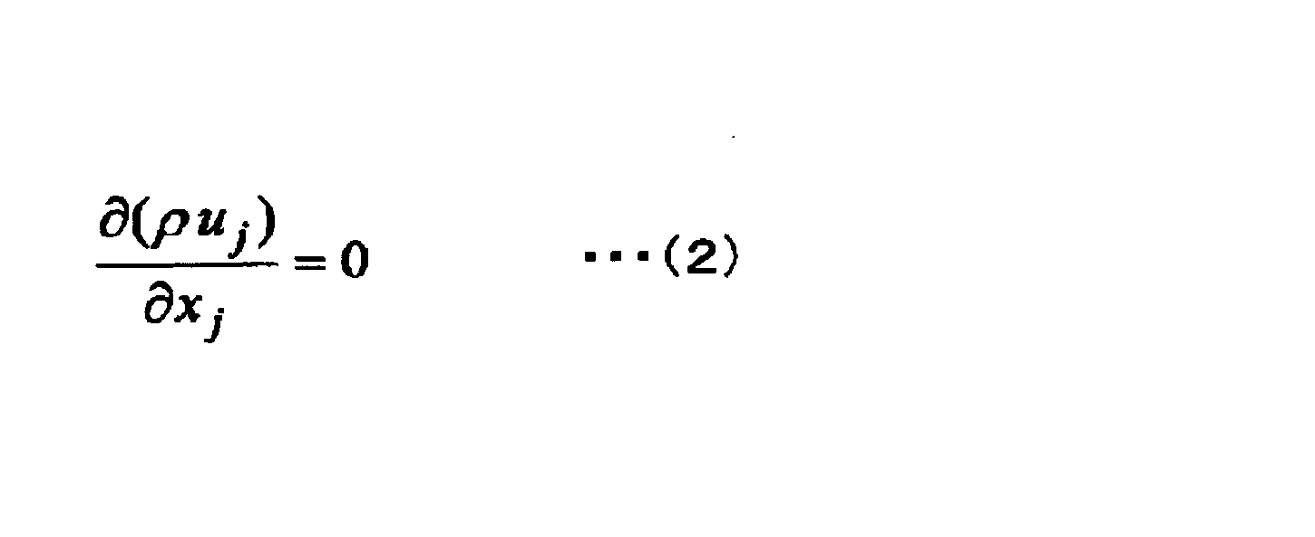
そして、式(1),(2)を、重み付き残差積分法に基づいて、分割領域のコントロールボリュームの体積に対して積分して示すと、式(1)が下式(3)のように示され、式(2)が下式(4)のように示される。
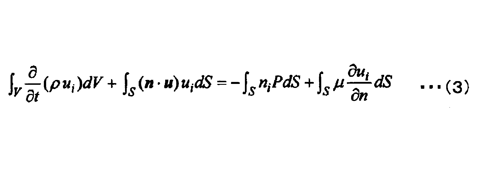
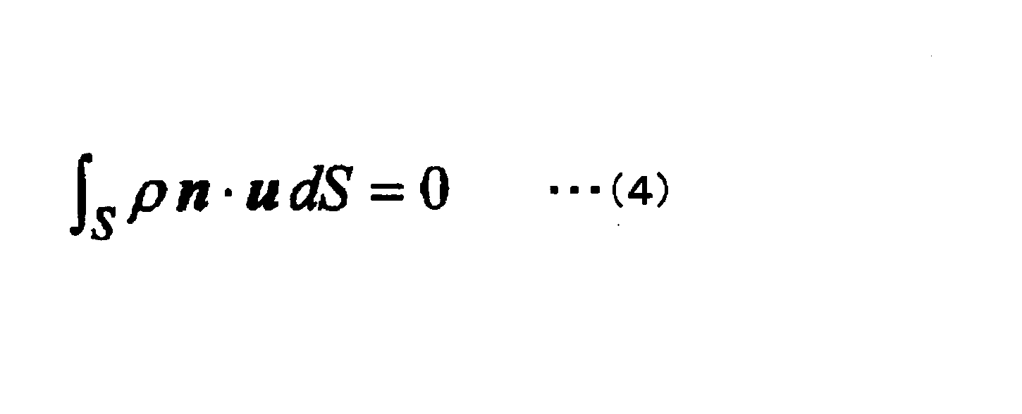
ここで、説明を簡単化するために、流体の密度ρと粘性係数μを定数とする。ただし、以下の定数化は、流体の物性値が、時間、空間、温度等によって変化する場合に対して拡張可能である。
そして、図1のコントロールポイントaについて、境界面Eの面積Sabについて離散化し、代数方程式による近似式に変換すると、式(3)が下式(5)、式(4)が下式(6)のように示される。
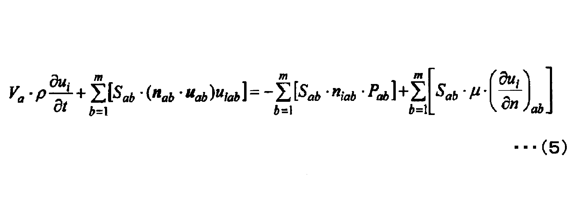

そして、式(5),(6)をVa(コントロールポイントaのコントロールボリュームの体積)で割ると、式(5)が下式(7)のように示され、式(6)が下式(8)のように示される。
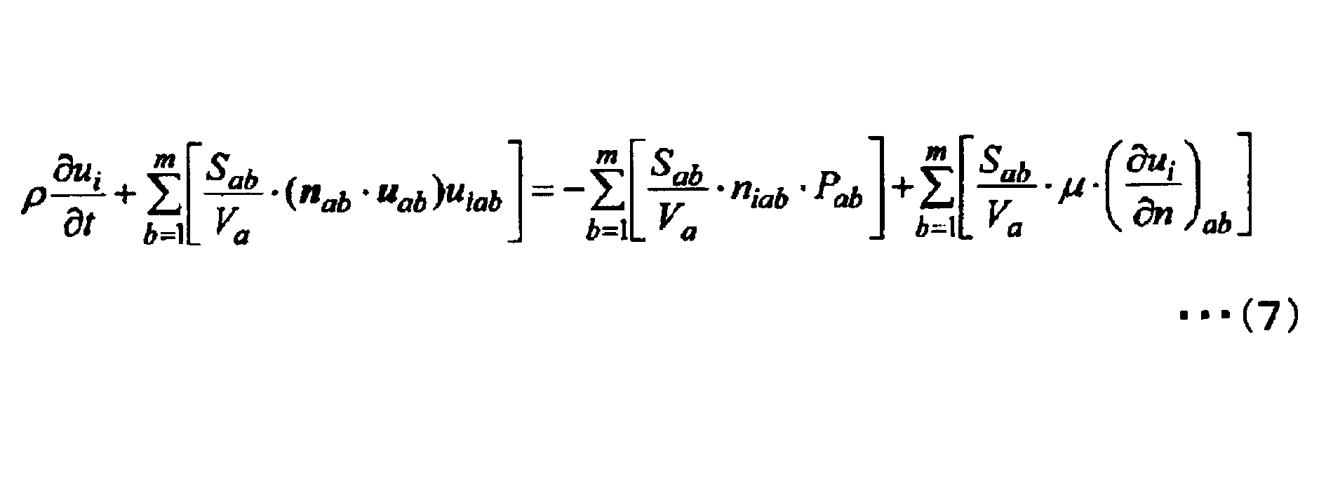


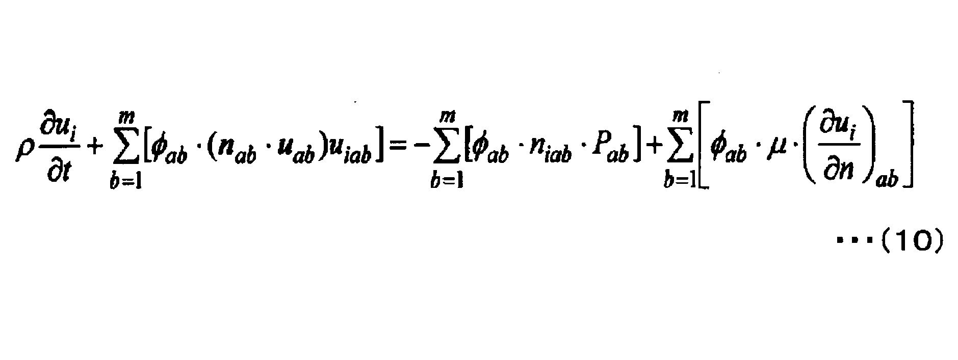
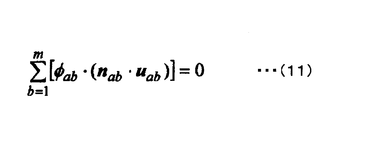
つまり、このような式(10)、(11)は、セル形状を規定する幾何学的形状を規定する量を必要としない量のみを使用して物理量が算出可能な、重み付き残差積分法に基づく演算式である。
このため、物理量計算(ソルバ処理)に先立って前述の第一計算用データモデルを作成し、物理量計算において当該第一計算用データモデルと、式(10)、(11)の離散化支配方程式とを用いることによって、物理量計算においてコントロールボリュームの幾何学的形状を規定する量を全く使用せずに、流速の計算を行うことができる。
このように、物理量計算において幾何学的形状を規定する量を全く使用せずに流速の計算が行えることから、第一計算用データモデルに幾何学的形状を規定する量を持たせる必要がなくなる。よって、第一計算用データモデルの作成にあたり、セルの幾何学的形状に縛られる必要がなくなるため、セルの形状を任意に設定することができる。このため、本数値解析手法によれば、前述のように3次元形状データの修正作業に対する規制を大幅に緩和することができる。
なお、実際に式(10)、(11)を解くにあたり、[u]ab、uiab、Pab等の境界面E上の物理量は、通常、線形補間によって補間される。例えば、コントロールポイントaの物理量をψa、コントロールポイントbの物理用をψbとすると、境界面E上の物理量ψabは、下式(12)によって求めることができる。
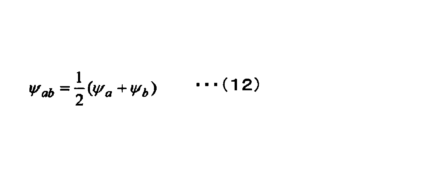
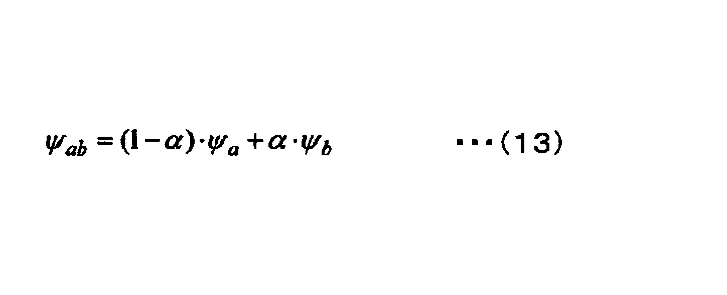
また、連続体モデルの方程式(ナビエ・ストークスの式等)には、式(1)に示すように、1階の偏導関数(偏微分)が含まれる。
ここで、連続体モデルの方程式の微係数を部分積分、ガウスの発散定理、あるいは一般化されたグリーンの定理を利用して、体積分を面積分に変換し、微分の次数を下げる。これによって1次微分は0次微分(スカラー量またはベクトル量)とすることができる。
例えば一般化されたグリーンの定理では、物理量をψとすると、下式(14)という関係が成り立つ。
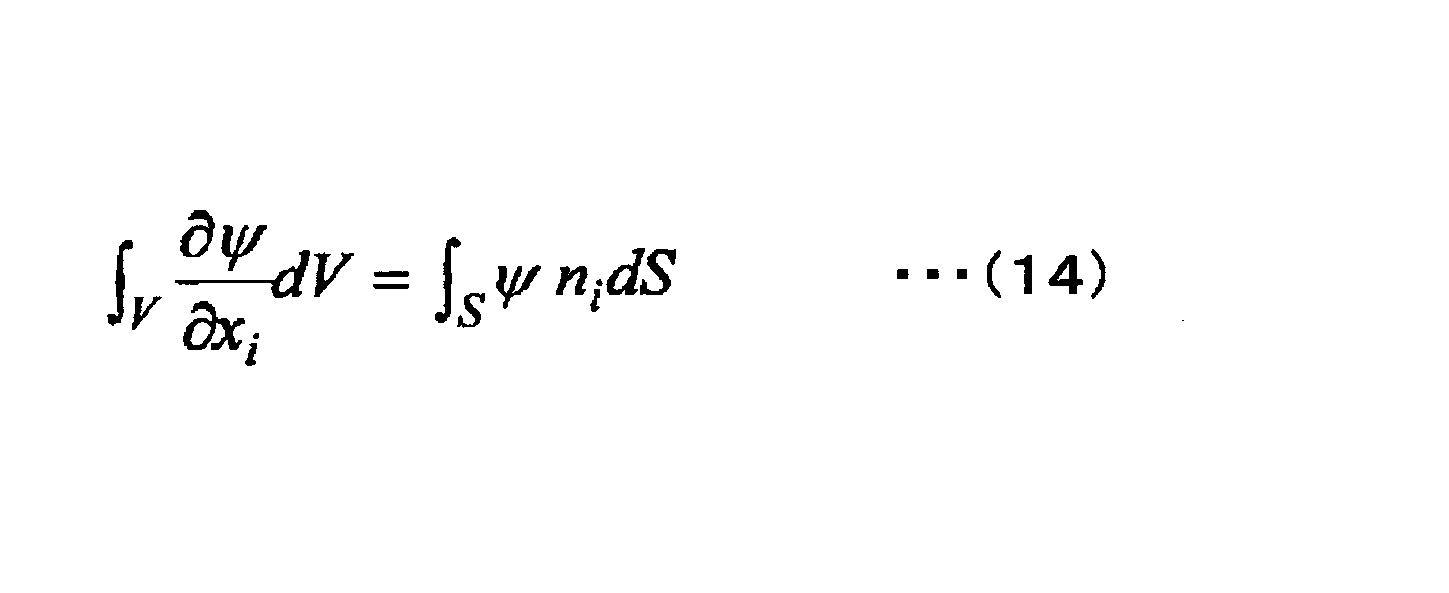
連続体モデルの方程式の1次微分項は、体積分から面積分の変換により、境界面上ではスカラー量またはベクトル量として取り扱われる。そして、これらの値は、前述の線形補間等によって、各コントロールポイント上の物理量から補間できる。
また、連続体モデルの方程式によっては、2階の偏導関数が含まれる場合もある。
式(14)の被積分関数をさらに1階微分した式は下式(15)となり、連続体モデルの方程式の2次微分項は、体積分から面積分の変換により境界面E上では下式(16)となる。
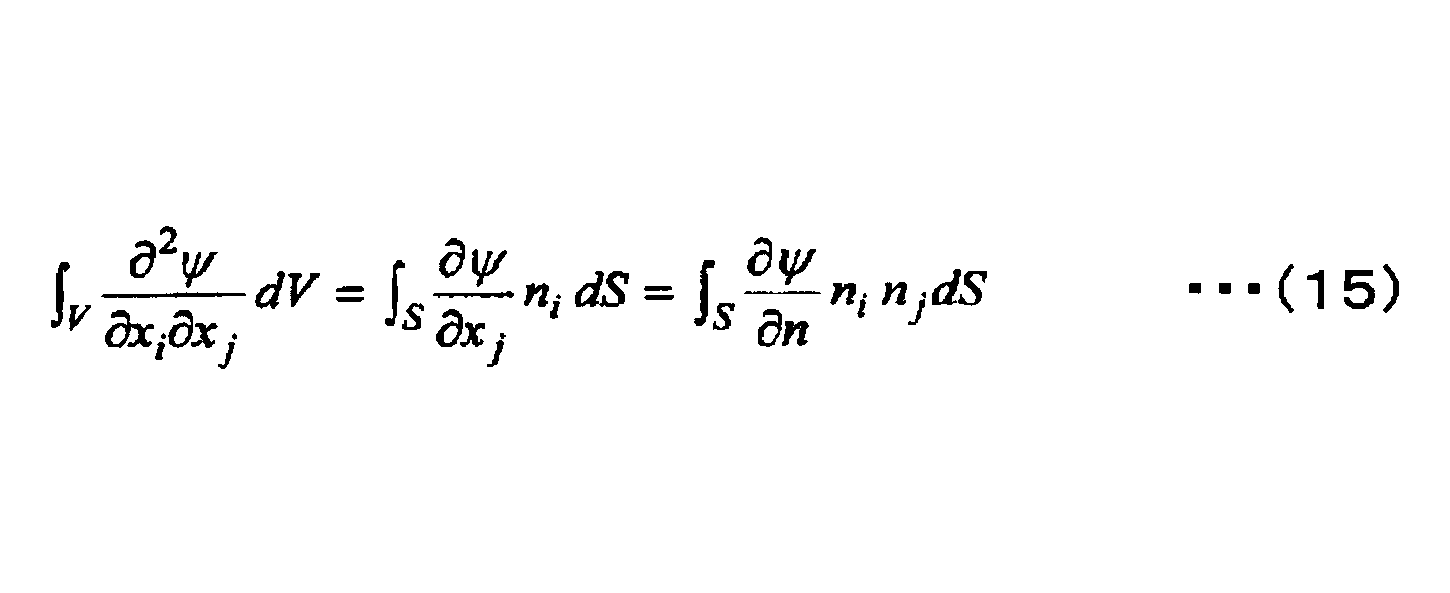
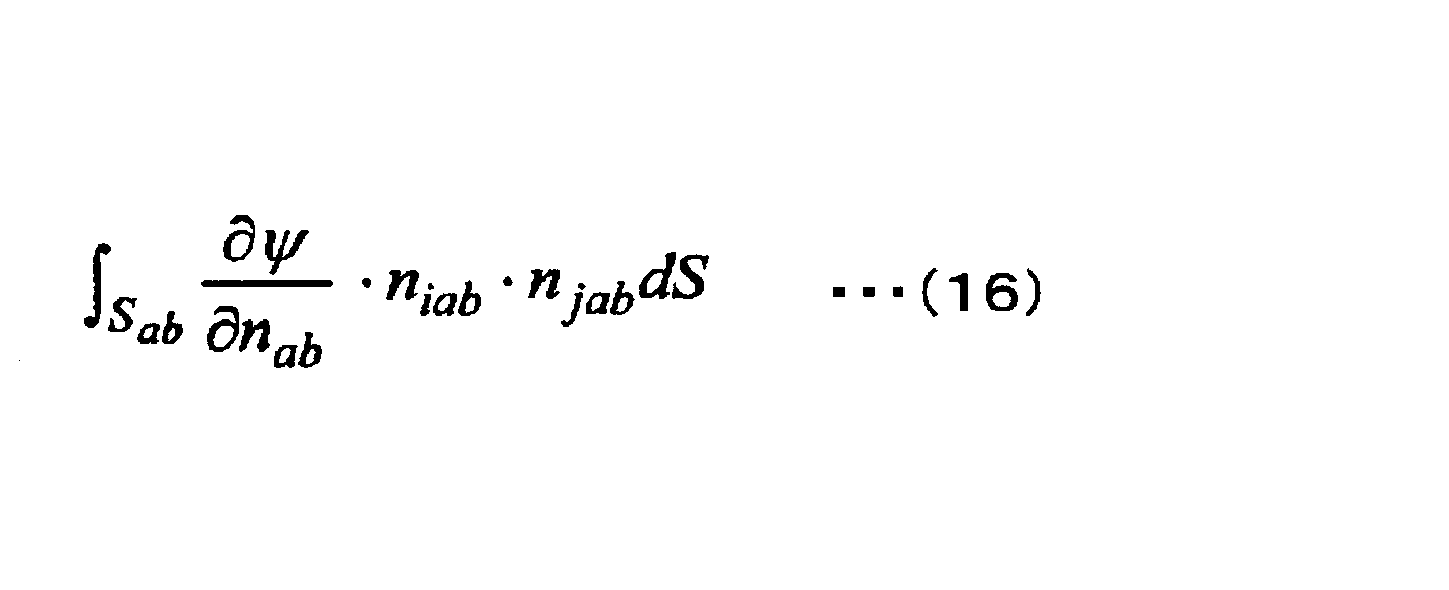
つまり、連続体モデルの方程式の2次微分項は、体積分から面積分の変換により、物理量ψの法線方向微分(Sabの法線[n]ab方向への微分)に、[n]の成分niab、njabを乗じた形となる。
ここで式(16)中の∂ψ/∂nabは、下式(17)と近似される。


すべての線形偏微分方程式は、定数と、1次、2次、その他の偏導関数に係数を乗じた項の線形和で表わされる。式(15)から式(19)において、物理量ψをψの1次偏導関数に置き換えると、より高次の偏導関数の体積分を、式(14)のように低次の偏導関数の面積分により求めることができる。この手順を、低次の偏微分から順次繰り返すと、線形偏微分方程式を構成するすべての項の偏導関数は、コントロールポイントの物理量ψと、式(12)又は式(13)で計算される境界面上のψであるψabと、式(18)で定義されるコントロールポイント間ベクトルから求められるコントロールポイント間距離と、境界面Eの面積Sab、境界面Eの法線ベクトルの成分niabとnjabから、すべて求めることができる。
本数値解析手法において物理量計算にあたり幾何学的形状を規定する量を必要としないことは前述した。このため、第一計算用データモデルの作成にあたり、コントロールボリュームの体積と、境界面の面積及び法線ベクトルとを、幾何学的形状を規定する量を使用しないで求めれば、式(10)と式(11)との離散化支配方程式を用いて、コントロールボリュームの幾何学的形状であるセルの幾何学的形状を全く使用せずに、流速の計算を行うことができる。
ただし、本数値解析手法においては、必ずしも、コントロールボリュームの体積と、境界面の面積及び法線ベクトルとを、コントロールボリュームの具体的な幾何学的形状を使用しないで求める必要はない。このように、ソルバ処理において幾何学的形状を規定する量を利用しないので、コントロールボリュームの具体的な幾何学的形状、具体的にはVertexとConnectivityとを利用するとしても、従来の有限要素法、有限体積法のような分割領域に関わる制約、すなわち分割領域の歪みや捩じれに対する制約がないため、前述のように容易に計算用データモデルの作成ができる。
なお、前述の説明においては、ナビエ・ストークスの式及び連続の式から重み付き残差積分法に基づいて導出した離散化支配方程式を用いる物理量の計算例について説明したが、本数値解析手法において用いられる離散化支配方程式はこれに限られるものではない。
つまり、種々の方程式(質量保存の方程式、運動量保存の方程式、エネルギ保存の方程式、移流拡散方程式、及び波動方程式等)から重み付き残差積分法に基づいて導出されると共に、幾何学的形状を規定する量を必要としない量のみを使用して物理量を算出可能な離散化支配方程式であれば本数値解析手法に用いることができる。
そして、このような離散化支配方程式の特性によって、従来の有限要素法や有限体積法のようにいわゆるメッシュを必要としない、メッシュレスでの計算が可能となる。また、たとえ、プリ処理において、セルの幾何学的形状を規定する量を利用するとしても、従来の有限要素法、有限体積法、ボクセル法のようなメッシュに対する制約がないため、第一計算用データモデルの作成に伴う作業負荷を軽減できる。
本実施形態では、質量保存の方程式、運動量保存の方程式、エネルギ保存の方程式、移流拡散方程式、及び波動方程式から、重み付き残差積分法に基づいて、幾何学的形状を規定する量を必要としない量のみを使用する離散化支配方程式が導出可能である。そのため、本数値解析手法において他の支配方程式を用いることができる。これについては、特許文献1に記載した理由と同様であるため、説明を省略する。
(集合領域を生成する処理)
次に、本数値解析手法の第二計算用データモデルを作成するための分割領域から集合領域を生成する処理について説明する。集合領域を生成する処理では、セルの集合和により集合領域を作成する。以下、集合領域は、ドメインと呼ぶこともある。ドメインが作成されることによって、解析領域はドメイン分割された状態となる。
次に、本数値解析手法の第二計算用データモデルを作成するための分割領域から集合領域を生成する処理について説明する。集合領域を生成する処理では、セルの集合和により集合領域を作成する。以下、集合領域は、ドメインと呼ぶこともある。ドメインが作成されることによって、解析領域はドメイン分割された状態となる。
図2で、集合領域を生成する処理では、解析領域内に自動生成されたコントロールボリューム(セル)を集合させ、新たに設定されたコントロールボリュームを、ドメインと定義する。ドメインは、コントロールボリュームであり、セルの集合和である。
図3に示される複数のドメインのうち、任意のドメインをドメインAとする。ドメインA内に存在するセルの総数をNVAとした場合、ドメインAの体積VAは式(20)で表され、ドメインAのコントロールポイントの座標ベクトル[r]Aは式(21)で表される。以下の式(20)、式(21)により、セルの集合和を計算し、ドメインを設定する。
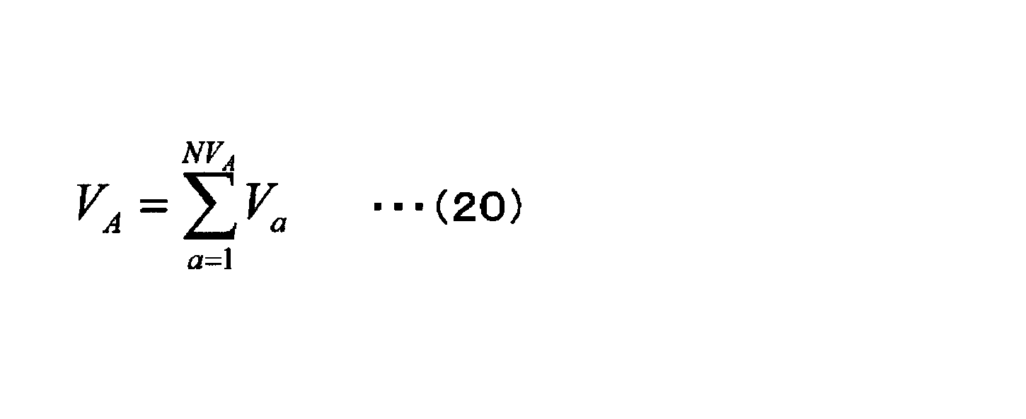

ここで、ドメインを設定した後に、設定したドメインを集合させることによって、新たにドメインを設定するようにしてもよい。
図4に示されるように、複数のドメインの集合和が設定される。図4に示される例では、細い線によってドメインが示されている。
図5に示されるように、ドメインを複数集合させることによって、新たにドメインが設定される。新たに設定されたドメインは、太線によって示されている。
新たに設定されたドメインも、コントロールボリュームであり、ドメインの集合和である。新たに設定されたドメインについても、式(20)、式(21)により、新たに設定されたドメインの体積と、新たに設定されたドメインのコントロールポイントの座標ベクトルが計算される。図6に示されるように、コントロールポイントが示される。そして、新たに設定されたドメインは、ドメインと同様に取り扱われる。
セルの集合和によって作成されたドメインをドメイン1とし、ドメイン1の集合和によって作成されたドメインをドメイン2とし、ドメイン2の集合和によって作成されたドメインをドメイン3とする。解析領域に自動生成されたコントロールボリューム(セル)に基づいて、ドメイン1、ドメイン2、ドメイン3、・・・、最終ドメインと階層構造型にドメインを設定できる。
要求される計算精度に合わせて、コントロールボリューム(セル)から、ドメイン1、ドメイン2、ドメイン3、・・・、最終ドメインと階層構造型にドメインを設定できる。ここで、ドメイン1から、ドメイン2やドメイン3を経ることなく、最終ドメインを設定してもよい。コントロールボリューム(セル)から、ドメイン1、ドメイン2、ドメイン3、・・・、最終ドメインと階層構造型にドメインを設定した場合や、ドメイン1から、ドメイン2を経ることなく、最終ドメインを設定した場合に、最初の解析領域の境界形状のセル分割精度が失われない。
従来の有限体積法や有限要素法では、初期の分割メッシュを集合させると、集合させたドメインの境界形状は複雑な多面となるため、計算を実行できない。具体的には、現状では、有限体積法では二十面体が限度であり、有限要素法では6面体を超える多面体の要素内補間関数を定義できない。このように、従来の方法においては、初期の分割メッシュを集合するという思想自体が存在しない。このことから、本実施形態は、分割領域から集合領域を形成することの動機づけも示唆もないところから着想され、従来の方法では不可能で、顕著な効果を奏する。
自動生成されたコントロールボリューム(セル)では、セル間でのマスバランス(質量保存)や運動量保存、エネルギ保存などの物理量の保存則を満足させながら数値解析ができる。従って、コントロールボリューム(セル)から、ドメイン1、ドメイン2、ドメイン3、・・・、最終ドメインと階層構造型に設定されたドメインでも、ドメイン1から、ドメイン2やドメイン3を経ることなく、最終ドメインと階層構造型に設定された場合でも、ドメイン間での物理量の保存則は満足される。
解析領域内に自動生成されたコントロールボリューム(セル)を集合させることによって、新たにドメインを設定するための、コントロールボリューム(セル)の集合方法について説明する。
図7に示されるように、解析領域を直交格子状の領域に粗く分割し、その直交格子内にコントロールポイントの座標が含まれるセルを集合させる。
図8に示されるように、解析領域内に、ドメインのコントロールポイントを設定する。ドメインのコントロールポイントから、予め指定された半径の球体内にコントロールポイントの座標が含まれるセルを集合させる。半径を徐々に拡大し、解析領域内のセルを全て、ドメインのいずれかに集合させる。
また、ボクセル法で、解析領域を包含する領域にボクセルを生成し、そのボクセルをドメインとしてもよい。この場合、ボクセル内にコントロールポイントの座標が含まれるセルを集合させる。
ここでは、セルの集合方法として、三例について説明したが、この例に限られない。例えば、ここに示した例以外の集合方法が使用されてもよい。
解析領域内に自動生成されたコントロールボリューム(セル)を、コントロールボリューム(セル)の集合方法にしたがって集合させることによって新たにドメインを設定した場合には、最初の解析領域の境界形状のセル分割精度が失われない。このため、解析領域内に自動生成されたコントロールボリューム(セル)を、コントロールボリューム(セル)の集合方法にしたがって集合させることによって新たに設定されたドメイン間で、物理量の保存則を満足させながら数値解析ができる。
(集合領域での第二計算用データモデルを生成する処理)
さらに、集合領域での第二計算用データモデルを生成する処理について説明する。
さらに、集合領域での第二計算用データモデルを生成する処理について説明する。
図9は、発明の数値解析手法の集合領域における境界面特性量の一例を示す概念図である。図9は解析領域を分割する複数の分割領域と、複数の集合領域とを表す。図9において、実線で囲まれたドメインA及びドメインBは、集合領域である。図9において、破線で囲まれた図形は分割領域である。例えば、セルR201~セルR208は、分割領域である。ドメインAは、セルR201~セルR208を含む複数の分割領域を集合して得られる集合領域である。境界面EABは、ドメインAとドメインBとの間において物理量の交換が行われる面であり、第二計算用データモデルにおける境界面に相当する。また、面積SABは、境界面EABの面積を示し、本実施形態における集合領域の境界面特性量の1つである。
[n]a1~[n]a8の各々は、境界面EABで互いに接するセル同士の境界面の特性を示す量である法線ベクトルである。
図10のドメインA及びドメインBは、図9のドメインA及びドメインBである。コントロールポイントAc及びコントロールポイントBcは、それぞれドメインA及びドメインBの内部に配置されている。
ドメインBに属し境界面EABに接するセルbの境界面の総数をNSABとすると、ドメインAとドメインBとの間の境界面の面積SABと、ドメインAとドメインBとの間の境界面の法線ベクトル[n]ABは、式(22)、式(23)で計算される。ここで、Sabは、ドメインBに属し境界面EABに接するセルbの境界面の面積である。
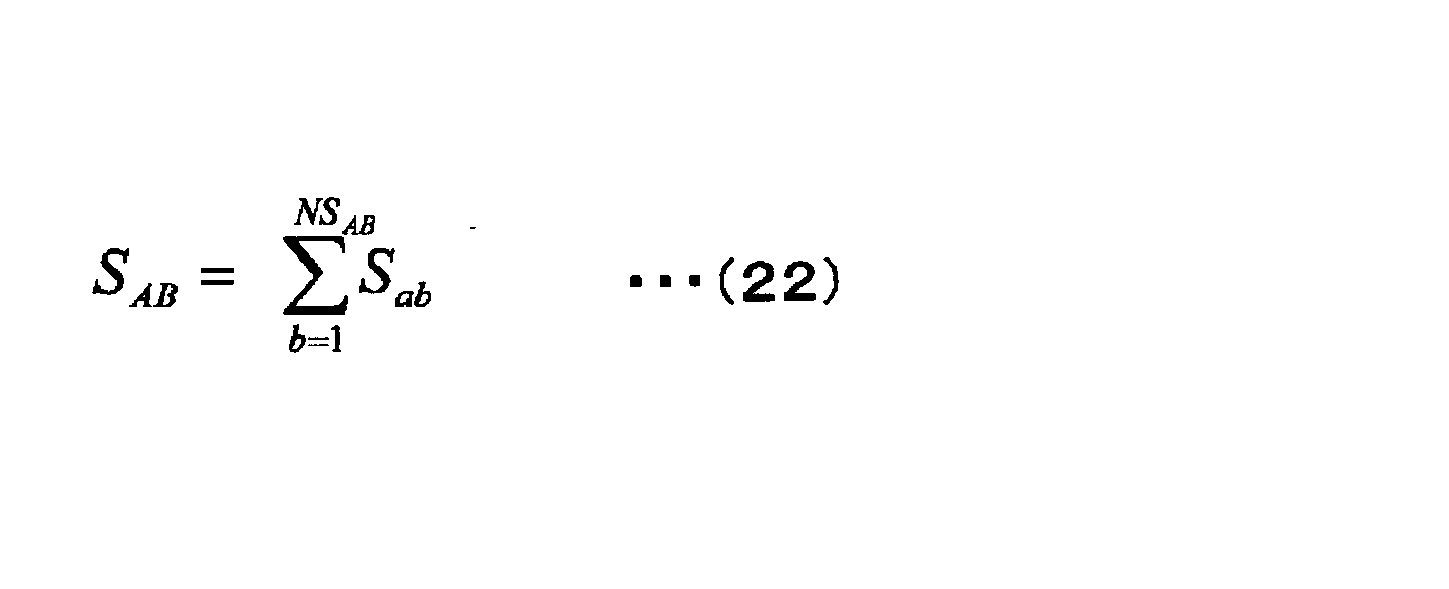
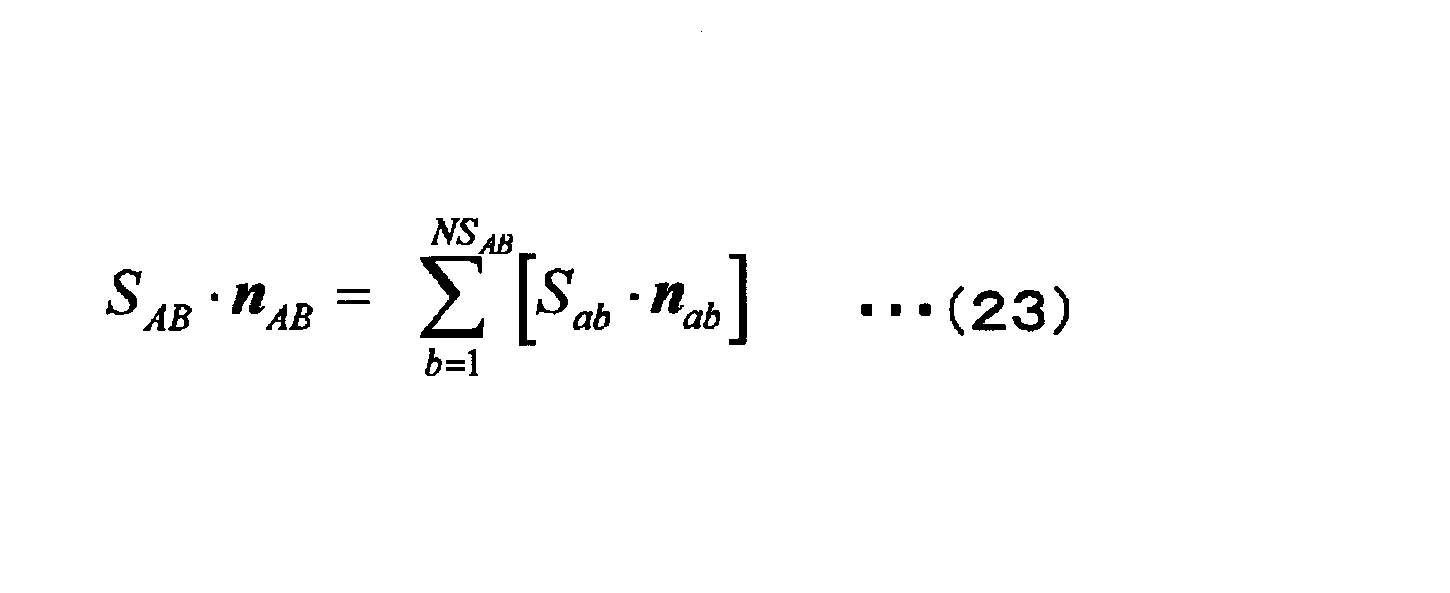
前述した数値解析手法では、解析領域内に自動生成されたコントロールボリューム(セル)を集合させることによって、ドメインを生成した。
さらに、数値解析手法では、セルaとセルbとの間の境界面Sabにおける境界面特性量(境界面の面積Sab、境界面の法線ベクトル[n]ab)を用いて、ドメインAとドメインBとの間の境界面SABに関して、集合和を計算することによって、ドメインAとドメインBとの間の境界面SABにおける境界面特性量(境界面の面積SAB、境界面の法線ベクトル[n]AB)を求めた。つまり、幾何学的形状を規定する量を使用しないセルによる連続体の数値解析手法を、ドメインに対しても全く同じ計算手法として適用した。
さらに、解析領域内に自動生成されたコントロールボリューム(セル)に基づいて、ドメイン1、ドメイン2、ドメイン3、・・・、最終ドメインと階層構造型にドメインを設定することができる。したがって、連続体の数値解析手法を、ドメイン1、ドメイン2、ドメイン3、・・・、最終ドメインと階層構造型に設定されたドメイン全てに対して適用できる。
コントロールボリューム(セル)から一度に最終ドメインを設定したときも、コントロールボリューム(セル)からドメイン1、ドメイン2、ドメイン3、・・・、最終ドメインと階層構造型にドメインを設定したときも、最初の解析領域の境界形状のセル分割精度は失われない。これは、熱流体解析のように伝熱面積を重要視する数値解析では、非常に大きなメリットである。
解析領域内に自動的に生成されたコントロールボリューム(セル)の分割数が、数10個~数1000個のオーダー以下の粗さの場合、その粗い分割数のセルを用いた数値解析は、解析結果に誤差を多く含むおそれがある。
一方、数1000万個~数億個以上のオーダーのセル分割による数値解析は、非常に高精度であるが、スーパーコンピュータを用いて行う計算レベルであり、大型のメモリ容量と、HDD容量との計算資源が必要であり、長大な計算時間、解析結果処理のための多大な計算コストの増大を招く。
しかし、数1000万個~数億セル以上のオーダーのセル分割に関しては、セルの自動生成だけなら、比較的低容量のメモリを備えるコンピュータで、短時間で実行できる。
そこで、数1000万個~数億個以上のオーダーのセル分割を、解析領域内で行い、そのセル分割に基づいて、ドメイン1、ドメイン2、ドメイン3、・・・、最終ドメインと階層構造型にドメイン分割を行うこともできる。ドメイン分割数が、数千~数万個のオーダーであれば、比較的低容量のメモリを備えるコンピュータで短時間に数値解析を実行できる。
この場合、セルを集合させたドメインの境界形状は非常に複雑な多面となるが、幾何学的形状を規定する量を使用しないセルによる連続体の数値解析手法を用いることによって、解析領域の境界形状のセル分割精度を維持した状態で、連続体の数値解析を、比較的低メモリのコンピュータで、解析結果に含まれる誤差を問題とならない程度に抑制しながら、短時間に実行できる。
次に、前述の第二計算用データモデルを用いて解析領域の集合領域における流速を求める物理量計算例について説明する。なお、ここでは、各集合コントロールポイントにおける流速を各集合領域における流速として求める。
第二計算用データモデルを用いる場合であっても、第一計算用データモデルを用いる場合と同様に、まずは、式(1)及び式(2)によって表されるナビエ・ストークスの式及び連続の式を重み付き残差積分法に基づいて集合領域の体積に対して積分する。
その結果、式(3)及び(4)が導出される。ただし、式(3)及び(4)において、第一計算用データモデルを用いる場合と異なり、Vが集合領域の体積を示し、∫VdVが集合領域の体積Vに関する積分を示し、Sが集合領域の面積を示し、∫SdSが集合領域の境界面Sに関する積分を示し、[n]が集合領域の境界面Sの法線ベクトルを示し、ni(i=1,2,3)が集合領域の境界面Sの法線ベクトル[n]の成分を示し、∂/∂nが集合領域の境界面Sの法線方向微分を示す。
第一計算用データモデルの場合と同様に、以下、説明を簡単化するために、流体の密度ρと粘性係数μを定数とする。ただし、第一計算用データモデルの場合と同様に、以下の定数化は、流体の物性値が、時間、空間、温度等によって変化する場合に対して拡張可能である。
集合コントロールポイントについて、図9と図10に示すように、境界面EABの面積SABについて離散化し、代数方程式による近似式に変換すると、式(3)が下式(24)、式(4)が下式(25)のように示される。

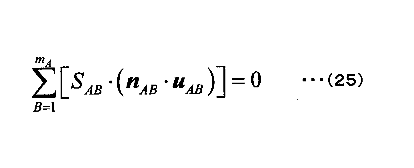
そして、式(24),(25)をVA(集合領域Aの体積)で割ると、式(24)が下式(26)のように示され、式(25)が下式(27)のように示される。
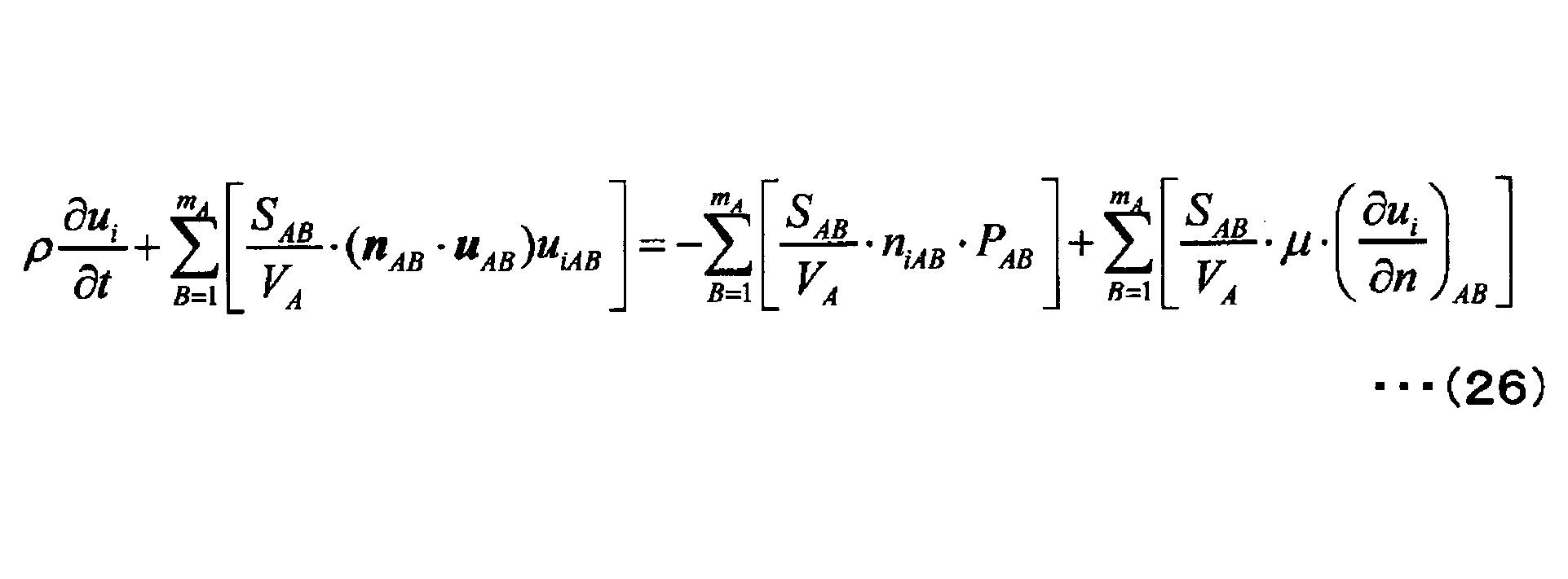
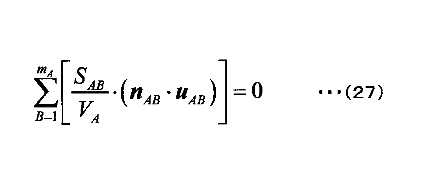

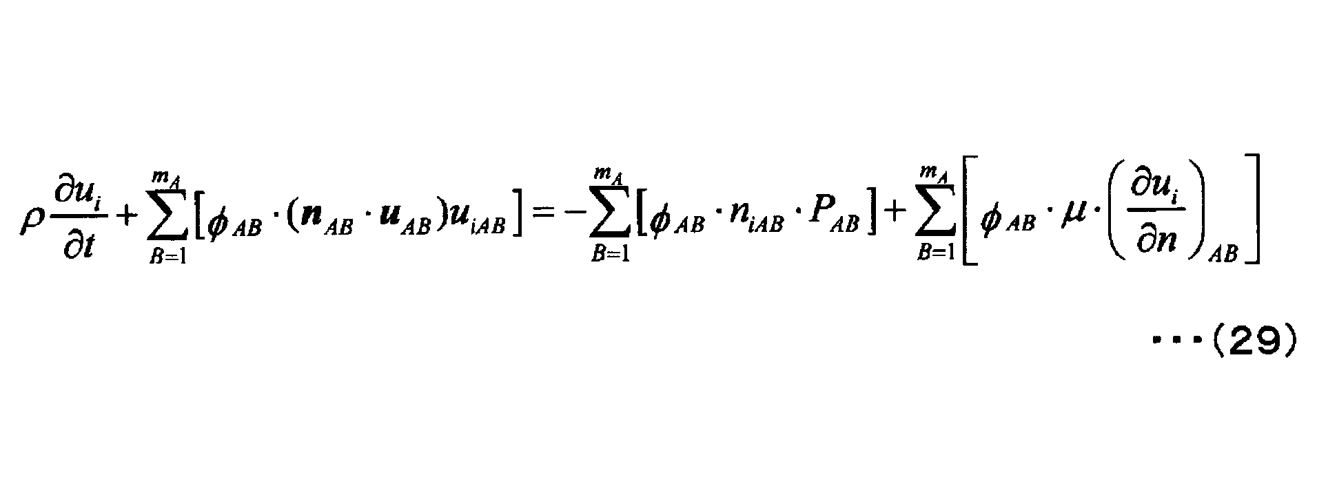
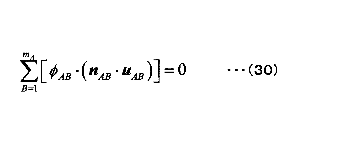
また、式(28)で定義されるφABも(面積/体積)という量であり、集合領域のコントロールボリュームの幾何学的形状を規定する量には無関係な量である。
つまり、このような式(29)、(30)は、集合領域の形状を規定するVertexとConnectivityを必要としない量のみを使用して物理量が算出可能な、重み付き残差積分法に基づく演算式である。
このため、物理量計算(ソルバ処理)に先立って前述の第二計算用データモデルを作成し、物理量計算において当該計算用データモデルと、式(29),(30)の離散化支配方程式とを用いることによって、物理量計算において集合領域の幾何学的形状を規定する量を全く使用せずに、流速の計算を行うことが可能である。
このように、物理量計算において集合領域の形状を規定するVertexとConnectivityとを全く使用せずに流速の計算が行えることから、第一計算用データモデルと同様に、第二計算用データモデルにおいても幾何学的形状を規定する量を持たせる必要がなくなる。
なお、実際に式(29),(30)を解くにあたり、[u]ABやPAB等の境界面EAB上の物理量は、第一計算用データモデルでの計算式(12)~(19)において、物理量Ψを分割領域のコントロールポイントの物理量から集合領域のコントロールポイントの物理量に置き換え、分割領域の境界面の面積と法線ベクトルを集合領域の境界面の面積(22)式と法線ベクトル(23)式に置き換え、分割領域のコントロールポイント間の距離(18)式において分割領域のコントロールポイントの位置(座標)ベクトルを集合領域のコントロールポイントの位置(座標)ベクトル(21)式に置き換えることで、第一計算用データモデルと同様に計算することができる。
次に、物理量計算にあたり、物理量の保存則が満足される条件について説明する。以下、まずは本数値解析における第一計算用データモデルを用いた計算において物理量の保存則が満足される条件を説明する。
第一計算用データモデルを用いた計算において、分割領域の質量保存則を表す連続の式(6)式におけるコントロールポイント間の分割領域の境界面の面積は、コントロールポイントa側から見てもコントロールポイントb側から見ても等しいとすると、コントロールポイント間の質量流束(ρ[n]・[u])・Sは、コントロールポイントa側とコントロールポイントb側で正負が逆で絶対値が等しくなる。従って、(6)式を解析領域内の全分割領域に対して総和を取ると、分割領域間の質量流束は差し引きゼロとなりキャンセルされ、計算する解析領域全体に対して、流入する質量と流出する質量が等しいことを示す。
よって、計算する解析領域全体についての質量保存則を満足するためには、分割領域の2つのコントロールポイント間の境界面の面積が一致するという条件及び分割領域の境界面の法線ベクトルが一方のコントロールポイント側から見た場合と他方のコントロールポイント側から見た場合とで正負が逆で絶対値が一致するという条件が必要である。
また、質量保存則を満足するためには、下式(31)に示される分割領域のコントロールボリュームの占める体積の総和が解析領域の全体積Vtotalと一致するという条件が必要である。なお、解析領域内の分割領域の総数はNである。
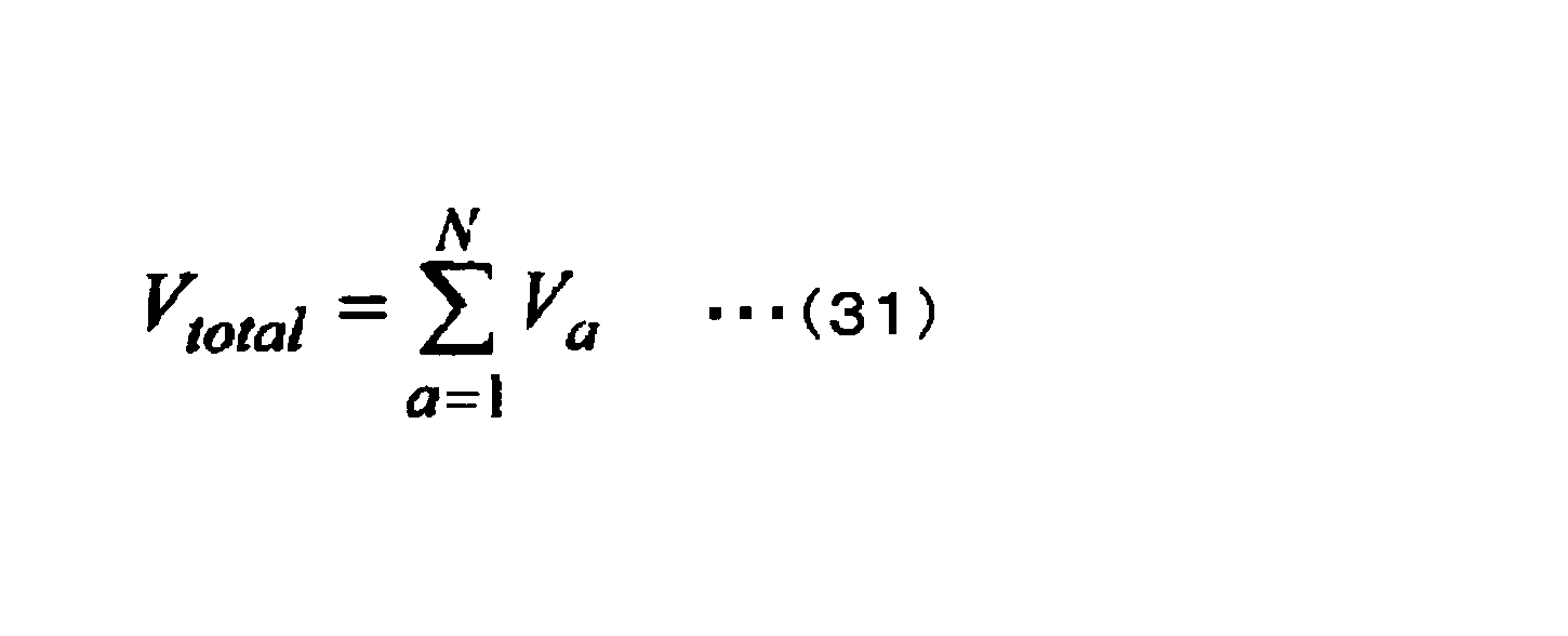
また、保存則を満たすためには、図13に示すように、分割領域のコントロールポイントaの占めるコントロールボリュームを考えた場合に、コントロールポイントaを通り、任意の向きの単位第一法線ベクトル[n]pを持つ無限に広い投影面Pを考えたときに下式(32)が成り立つという条件が必要である。単位法線ベクトルは、単位長さの法線ベクトルである。
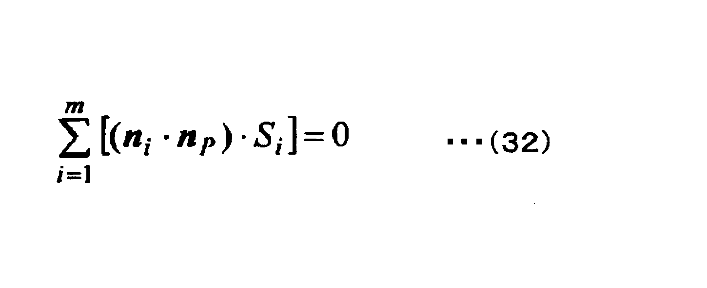
式(32)は、コントロールボリュームを構成する多面体が、閉包空間を構成することを示す。この式(32)は、コントロールボリュームを構成する多面体の一部が凹んでいる場合であっても成立する。
また、多面体の1つの面を微小面dSとし、mを∞とする極限を取ると、下式(33)となり、図14に示すような閉包曲面体についても成り立つことが分かる。
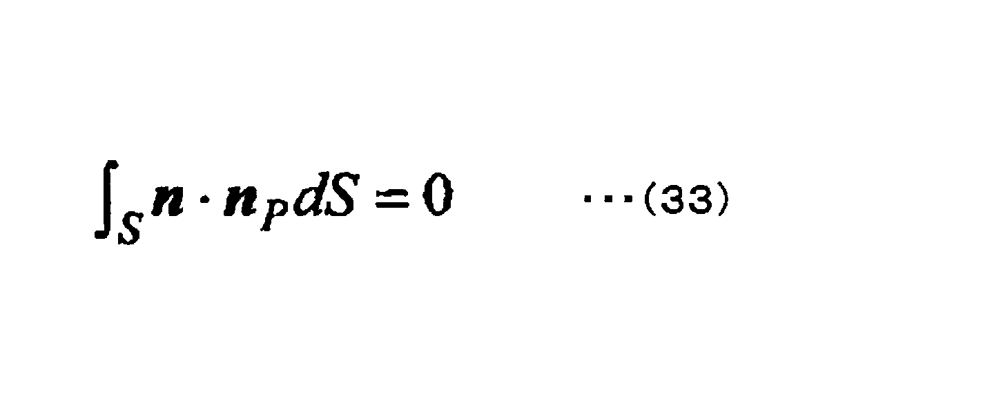
そして、一般化されたグリーンの定理は、連続体の離散化のための基本となる定理である。したがって、グリーンの定理にしたがって体積分を面積分に変形し離散化させる場合において、保存則を満足させるためには式(32)が成り立つという条件は必須となる。
このように、前述の第一計算用データモデル及び物理量計算を用いて数値解析を行う際に、物理量の保存則が満足されるためには、以下の3つの条件(以下「第一計算用条件」という。)が必要となる。
(a1)全コントロールポイントのコントロールボリュームの体積(全分割領域の体積)の総和が解析領域の体積と一致する。
(b1)2つのコントロールポイント間の境界面の面積が一致する及び第一法線ベクトルが一方のコントロールポイント側(境界面を挟む一方の分割領域)から見た場合と他方のコントロールポイント側(境界面を挟む他方の分割領域)から見た場合とで絶対値が一致する。
(c1)コントロールポイントを通り(分割領域を通り)、任意の向きの単位第一法線ベクトル[n]pを持つ無限に広い投影面Pを考えたときに式(32)が成り立つ。
第二計算用データモデルを用いた計算において、集合領域の質量保存則を表す連続の式(25)式における集合コントロールポイント間の集合領域の境界面の面積は、集合コントロールポイントA側から見てもコントロールポイントB側から見ても等しいとすると、集合コントロールポイント間の質量流束は、集合コントロールポイントA側と集合コントロールポイントB側で正負が逆で絶対値が等しくなる。従って、(25)式を解析領域内の全集合領域に対して総和を取ると、集合領域間の質量流束は差し引きゼロとなりキャンセルされ、計算する解析領域全体に対して、流入する質量と流出する質量が等しいことを示す。
よって、計算する解析領域全体についての質量保存則を満足するためには、集合領域の2つのコントロールポイント間の境界面の面積が一致するという条件及び集合領域の境界面の法線ベクトルが一方のコントロールポイント側から見た場合と他方のコントロールポイント側から見た場合とで正負が逆で絶対値が一致するという条件が必要である。
また、質量保存則を満足するためには、下式(34)に示される集合領域のコントロールボリュームの占める体積の総和が解析領域の全体積Vtotalと一致するという条件が必要である。解析領域内の集合領域の総数をNDとする。

また、保存則を満たすためには、図15に示すように、集合コントロールポイントAの占める集合コントロールボリュームを考えた場合に、集合コントロールポイントAを通り、任意の向きの単位第二法線ベクトル[N]Pを持つ無限に広い投影面Pdを考えたときに下式(35)が成り立つという条件が必要である。単位第二法線ベクトルは、単位長さの第二法線ベクトルである。
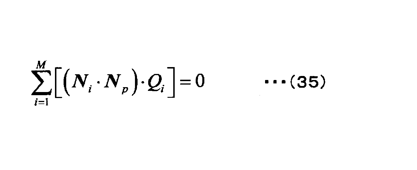
式(35)は、集合コントロールボリュームを構成する多面体が、閉包空間を構成することを示す。この式(35)は、集合コントロールボリュームを構成する多面体の一部が凹んでいる場合であっても成立する。
また、多面体の1つの面を微小面dQとし、Mを∞とする極限を取ると、下式(36)となり、図16に示すような閉包曲面体についても成り立つことが分かる。
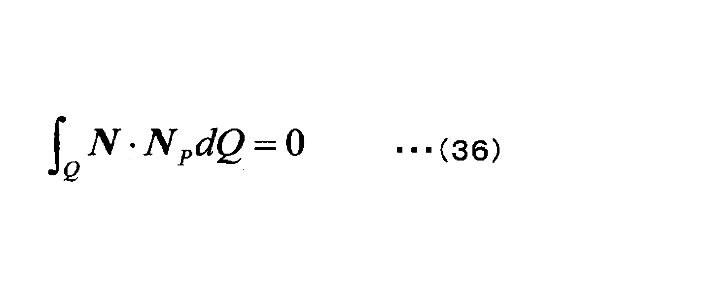
そして、一般化されたグリーンの定理は、連続体の離散化のための基本となる定理である。したがって、グリーンの定理にしたがって体積分を面積分に変形し離散化させる場合において、保存則を満足させるためには式(35)が成り立つという条件は必須となる。
このように、前述の第二計算用データモデル及び物理量計算を用いて数値解析を行う際に、物理量の保存則が満足されるためには、以下の3つの条件(以下「第二計算用条件」という。)が必要となる。
(a2)全集合領域の体積の総和が解析領域の体積と一致する。
(b2)2つの集合コントロールポイント間の境界面の面積が一致する及び第二法線ベクトルが一方の集合コントロールポイント側(境界面を挟む一方の集合領域)から見た場合と他方の集合コントロールポイント側(境界面を挟む他方の集合領域)から見た場合とで絶対値が一致する。
(c2)集合コントロールポイントを通り(集合領域を通り)、任意の向きの単位集合第二法線ベクトル[N]Pを持つ無限に広い投影面Pdを考えたときに上式(35)が成り立つ。
つまり、保存則を満足させる場合には、これらの条件を満足するように第一及び第二計算用データモデルを作成する必要がある。ただし、前述のように本数値解析手法においては、計算用データモデルの作成にあたり、分割領域のセル形状を任意に変形することができ、その分割領域セルを集合和させることにより集合領域を作成することから、容易に上記3つの条件を満足するように第一及び第二計算用データモデルを作成することができる。
このように、本数値解析手法においては、第一計算用データモデルだけでなく、第一計算用データモデルよりも解析領域の分割数が少ない第二計算用データモデルも保存則を満足する。そのため、本数値解析手法は、解析領域の分割数が少なくても解析精度が悪くならない、という特徴を有する。
なお、前述の説明においては、ナビエ・ストークスの式及び連続の式から重み付き残差積分法に基づいて導出した離散化支配方程式を用いる物理量の計算例について説明したが、本数値解析手法において用いられる離散化支配方程式はこれに限られるものではない。
つまり、種々の方程式(質量保存の方程式、運動量保存の方程式、エネルギ保存の方程式、移流拡散方程式、及び波動方程式等)から重み付き残差積分法に基づいて導出されると共に、幾何学的形状を規定する量を必要としない量のみを使用して物理量を算出可能な離散化支配方程式であれば本数値解析手法に用いることができる。
そして、このような離散化支配方程式の特性によって、従来の有限要素法や有限体積法のようにいわゆるメッシュを必要としない、メッシュレスでの計算が可能となる。また、たとえ、プリ処理において、セルの幾何学的形状を規定する量を利用するとしても、従来の有限要素法、有限体積法、ボクセル法のようなメッシュに対する制約がないため、計算用データモデルの作成に伴う作業負荷を軽減できる。具体的には、従来の有限要素法や有限体積法等に基づくソフトによる幾何学的形状を規定する量に基づいて、各分割領域の体積と隣り合う前記分割領域同士の特性を示す分割領域特性量を求めてもよい。
本実施形態では、質量保存の方程式、運動量保存の方程式、エネルギ保存の方程式、移流拡散方程式、及び波動方程式から、重み付き残差積分法に基づいて、幾何学的形状を規定する量を必要としない量のみを使用する離散化支配方程式が導出可能である。そのため、本数値解析手法において他の支配方程式を用いることができる。これについては、特許文献1に記載した理由と同様であるため、説明を省略する。
なお、特許文献1では、解析領域が分割領域によって分割される場合について離散化支配方程式が導出可能であることを説明するが、解析領域が集合領域によって分割される場合についても、同様に離散化支配方程式が導出可能である。
(適用例)
以下の説明においては、本実施形態に係る物理量計算方法を含む数値解析方法と、本実施形態に係る物理量計算プログラムを含む数値解析プログラムと、本実施形態に係る物理量計算装置を含む数値解析装置との具体的な適用例について説明する。
以下の説明においては、本実施形態に係る物理量計算方法を含む数値解析方法と、本実施形態に係る物理量計算プログラムを含む数値解析プログラムと、本実施形態に係る物理量計算装置を含む数値解析装置との具体的な適用例について説明する。
また、以下の具体的な適用例においては、自動車のキャビン空間における空気の流速を数値解析によって求める場合について説明する。
図17は、本実施形態の数値解析装置Aのハードウェア構成を概略的に示すブロック図である。
この図に示すように、本実施形態の数値解析装置Aは、パーソナルコンピュータやワークステーション等のコンピュータによって構成され、CPU1、記憶装置2、DVDドライブ3、入力装置4、出力装置5、及び通信装置6を備えている。
CPU1は、記憶装置2、DVDドライブ3、入力装置4、出力装置5、及び通信装置6と電気的に接続されており、これらの各種装置から入力される信号を処理すると共に、処理結果を出力する。なお、CPU1は、演算部1opの具体例である。
記憶装置2は、メモリ等の内部記憶装置及びハードディスクドライブ等の外部記憶装置によって構成されており、CPU1から入力される情報を記憶すると共にCPU1から入力される指令に基づいて記憶した情報を出力する。
そして、本実施形態において記憶装置2は、プログラム記憶部2aとデータ記憶部2bとを備えている。
プログラム記憶部2aは、数値解析プログラムPを記憶している。この数値解析プログラムPは、所定のOS(Operating System)において実行されるアプリケーションプログラムであり、コンピュータから構成される本実施形態の数値解析装置Aを、数値解析を行うように機能させる。そして、演算部1opが数値解析プログラムPを実行することによって、本実施形態の数値解析装置Aの各機能が実現される。
そして、図17に示すように、数値解析プログラムPは、プリ処理プログラムP1と、ソルバ処理プログラムP2と、ポスト処理プログラムP3とを有している。
プリ処理プログラムP1は、ソルバ処理を実行するための前処理(プリ処理)を本実施形態の数値解析装置Aに実行させ、本実施形態の数値解析装置Aを第一計算用データモデル作成部として機能させることによって第一計算用データモデルを作成させる。また、プリ処理プログラムP1は、本実施形態の数値解析装置Aを第二計算用データモデル作成部として機能させることによって第二計算用データモデルを作成させる。また、プリ処理プログラムP1は、本実施形態の数値解析装置Aに、ソルバ処理を実行するにあたり必要となる条件の設定を実行させ、さらには上記計算用データモデルや設定された条件を纏めたソルバ入力データファイルFの作成を実行させる。なお、プリ処理プログラムP1は、本実施形態の数値解析装置Aを第一計算用データモデル作成部として機能させ、第一計算用データモデルが作成された後、本実施形態の数値解析装置Aを第二計算用データモデル作成部として機能させる。
プリ処理プログラムP1は、本実施形態の数値解析装置Aを第一計算用データモデル作成部及び第二計算用データモデル作成部として機能させる場合に、まず本実施形態の数値解析装置Aに対して、自動車のキャビン空間を含む3次元形状データを取得させ、この取得させた3次元形状データに含まれる自動車のキャビン空間を示す解析領域の作成を実行させる。
なお、後に詳説するが、本実施形態においては、ソルバ処理において、前述の本実施形態を用いた数値解析手法にて説明した離散化支配方程式を用いる。前述の本実施形態を用いた数値解析手法にて説明した離散化支配方程式とは、具体的には、幾何学的形状を規定する量を必要としない量のみを使用すると共に重み付き残差積分法に基づいて導出された離散化支配方程式である。このため、第一計算用データモデル及び第二計算用データモデルの作成にあたり、保存則を満たす条件の下、分割領域の形状、分割領域に基づく集合領域の形状及び解析領域の形状を任意に変更できる。よって、3次元形状データに含まれる自動車のキャビン空間の修正あるいは変更作業は簡易的なもので充分となる。そこで、本実施形態においてプリ処理プログラムP1は、本実施形態の数値解析装置Aに対して、取得させた3次元形状データに含まれる自動車のキャビン空間に存在する穴や隙間に、微小な閉曲面を覆いかぶせるラッピング処理によって修繕する処理を実行させる。
その後、プリ処理プログラムP1は、本実施形態の数値解析装置Aに対して、複数の分割領域に分割する処理で説明したように分割領域を形成し、ラッピング処理等により修繕されたキャビン空間の全領域を含む解析領域の作成を実行させる。続いて、プリ処理プログラムP1は、本実施形態の数値解析装置Aに対して作成された分割領域のうちキャビン空間から食み出した領域をカットすることによって、キャビン空間を示す解析領域の作成を実行させる。ここでも、ソルバ処理において前述の離散化支配方程式を用いることから、解析領域のうちキャビン空間から食み出した領域を容易にカットすることができる。
これにより、ボクセル法のように、外部空間との境界が階段状になることがなく、また、ボクセル法のカットセル法のような外部空間の境界付近の解析領域の形成に対して、経験や試行錯誤を要する非常に膨大な手作業を伴う特別な修正または処理を必要としない。そのため、本実施形態では、ボクセル法で問題となる外部空間との境界の処理に関わる問題がない。
なお、本実施形態においては、後述のようにキャビン空間とカットした領域との隙間に新たな任意形状の分割領域を充填することによって、直交格子形状のみによらない分割領域で解析領域が構成されるようにし、さらには解析領域に分割領域を重なることなく充填させている。
次に、プリ処理プログラムP1は、本実施形態の数値解析装置Aを第一計算用データモデル作成部として機能させる場合に、本実施形態の数値解析装置Aに対して、作成させたキャビン空間を示す解析領域に含まれる分割領域の各々の内部に対して1つのコントロールポイントを仮想的に配置する処理を実行させ、コントロールポイントの配置情報、及び各コントロールポイントが占めるコントロールボリュームの体積データを記憶させる。
また、プリ処理プログラムP1は、本実施形態の数値解析装置Aを第一計算用データモデル作成部として機能させる場合に、本実施形態の数値解析装置Aに対して、上記分割領域同士の境界面である境界面の面積及び第一法線ベクトルの算出を実行させ、これらの境界面の面積及び第一法線ベクトルを記憶させる。
また、プリ処理プログラムP1は、本実施形態の数値解析装置Aを第一計算用データモデル作成部として機能させる場合に、コントロールボリューム又はコントロールポイントの結合情報(link)を作成させ、このlinkを記憶させる。
そして、プリ処理プログラムP1は、本実施形態の数値解析装置Aに対して、上記各コントロールポイントが占めるコントロールボリュームの体積と、境界面の面積及び第一法線ベクトルと、分割領域の配置情報を表すコントロールポイントの配置情報と、linkとを纏めさせて第一計算用データモデルを作成させる。配置情報が示す配置は、例えば座標を用いて示されてもよい。
プリ処理プログラムP1は、本実施形態の数値解析装置Aを第二計算用データモデル作成部として機能させる場合に、本実施形態の数値解析装置Aに対して、作成された第一計算用データモデルを用いて、図7あるいは図8に示す方法でコントロールボリューム(セル)を集合させ、キャビン空間を示す解析領域内に、集合領域を生成する。
次に、プリ処理プログラムP1は、本実施形態の数値解析装置Aを第二計算用データモデル作成部として機能させる場合に、本実施形態の数値解析装置Aに対して、作成させたキャビン空間を示す解析領域に含まれる集合領域の各々の内部に対して1つの集合コントロールポイントを仮想的に配置する処理を実行させ、集合コントロールポイントの配置情報、及び各集合コントロールポイントが配置されたドメインの体積データを記憶させる。
プリ処理プログラムP1は、上記集合コントロールポイントを仮想的に配置する処理において、本実施形態の数値解析装置Aにたいして、集合コントロールポイント算出処理を実行させることで、各集合コントロールポイントを配置する箇所を示す情報を取得する。集合コントロールポイント算出処理は、本実施形態の数値解析装置Aが第一計算用データモデルが有するコントロールボリュームの体積とコントロールポイントの配置情報とを取得し、式(20)及び式(21)の計算を行うことで、集合コントロールポイントの配置箇所を算出する処理である。
また、プリ処理プログラムP1は、本実施形態の数値解析装置Aを第二計算用データモデル作成部として機能させる場合に、本実施形態の数値解析装置Aに対して、上記集合領域同士の境界面の面積及び第二法線ベクトルの算出(以下「集合領域境界面特性量算出処理」という。)を実行させ、これらの境界面の面積及び第二法線ベクトルを記憶させる。
集合領域境界面特性量算出処理は、本実施形態の数値解析装置Aが第一計算用データモデルが有する境界面の面積と第一法線ベクトルとの情報を取得し、式(22)及び式(23)の計算を実行することで、集合領域同士の境界面の面積及び第二法線ベクトルを算出する処理である。
また、プリ処理プログラムP1は、本実施形態の数値解析装置Aを第二計算用データモデル作成部として機能させる場合に、ドメイン又は集合コントロールポイントの結合情報(link)を作成させ、このlinkを記憶させる。
そして、プリ処理プログラムP1は、本実施形態の数値解析装置Aに対して、上記各集合コントロールポイントが配置されたドメインの体積と、境界面の面積及び第二法線ベクトルと、集合領域の配置情報を表す集合コントロールポイントの配置情報と、linkとを纏めさせて第二計算用データモデルを作成させる。配置情報が示す配置は、例えば座標を用いて示されてもよい。
また、プリ処理プログラムP1は、本実施形態の数値解析装置Aに、前述のソルバ処理を実行するにあたり必要となる条件の設定を行わせる場合には、物性値の設定、境界条件の設定、初期条件の設定、計算条件の設定を行わせる。
ここで、物性値とは、キャビン空間における空気の密度、粘性係数等である。
境界条件とは、コントロールポイント間の物理量の交換の法則を規定する条件であり、、本実施形態においては前述した式(10)で示されるナビエ・ストークスの式に基づく離散化支配方程式、及び式(11)で示される連続の式に基づく離散化支配方程式である。
また、境界条件には、キャビン空間と外部空間との境界面に臨む集合領域を示す情報が含まれる。
初期条件とは、ソルバ処理を実行する際の最初の物理量を示すものであり、各分割領域及び集合領域の流速の初期値である。
計算条件とは、ソルバ処理における計算の条件であり、例えば反復回数や収束基準である。
また、プリ処理プログラムP1は、本実施形態の数値解析装置Aに、GUI(Graphical User Interface)を形成させる。より詳細には、プリ処理プログラムP1は、出力装置5が備えるディスプレイ5aに対してグラフィックを表示させると共に、入力装置4が備えるキーボード4aやマウス4bによって操作が可能な状態とさせる。
ソルバ処理プログラムP2(物理量計算プログラム)は、本実施形態の数値解析装置Aにソルバ処理を実行させるものであり、本実施形態の数値解析装置Aを物理量計算装置として機能させる。
そして、ソルバ処理プログラムP2は、本実施形態の数値解析装置Aを物理量計算部として機能させる場合に、ソルバ入力データファイルFを用いて、解析領域における物理量を数値計算させる。
そして、ソルバ処理プログラムP2は、本実施形態の数値解析装置Aを物理量計算部として機能させる場合に、本実施形態の数値解析装置Aに対して、ソルバ入力データファイルFに含まれるナビエ・ストークスの式及び連続の式の離散化係数行列の作成を実行させると共に、マトリックス形成用のデータテーブルの作成を実行させる。
また、ソルバ処理プログラムP2は、本実施形態の数値解析装置Aを物理量計算部として機能させる場合に、本実施形態の数値解析装置Aに対して、前述した式(29)で示されるナビエ・ストークスの式に基づく離散化支配方程式、及び前述した式(30)で示される連続の式に基づく離散化支配方程式から、下式(37)で示すマトリックス計算用の大規模疎行列方程式の組み上げを実行させる。
なお、ソルバ処理プログラムP2は、集合領域から作成される第二計算用データモデルを入力とする数値計算だけでなく、分割領域から作成される第一計算用データモデルを入力とする数値計算を実行することもできる。この場合は、本実施形態の数値解析装置Aに対して、前述した式(10)で示されるナビエ・ストークスの式に基づく離散化支配方程式、及び前述した式(11)で示される連続の式に基づく離散化支配方程式から、下式(37)で示すマトリックス計算用の大規模疎行列方程式の組み上げを実行させる。

また、ソルバ処理プログラムP2は、上記離散化支配方程式に非圧縮性等の付帯条件が存在する場合には、本実施形態の数値解析装置Aに対して、この付帯条件の行列方程式への組み上げを実行させる。
そして、ソルバ処理プログラムP2は、本実施形態の数値解析装置Aに対して、CG法(共役勾配法)等による行列方程式の解の計算、当該解の下式(38)を用いた解のアップデート、収束条件の判定を実行させ、最終的な計算結果を取得させる。
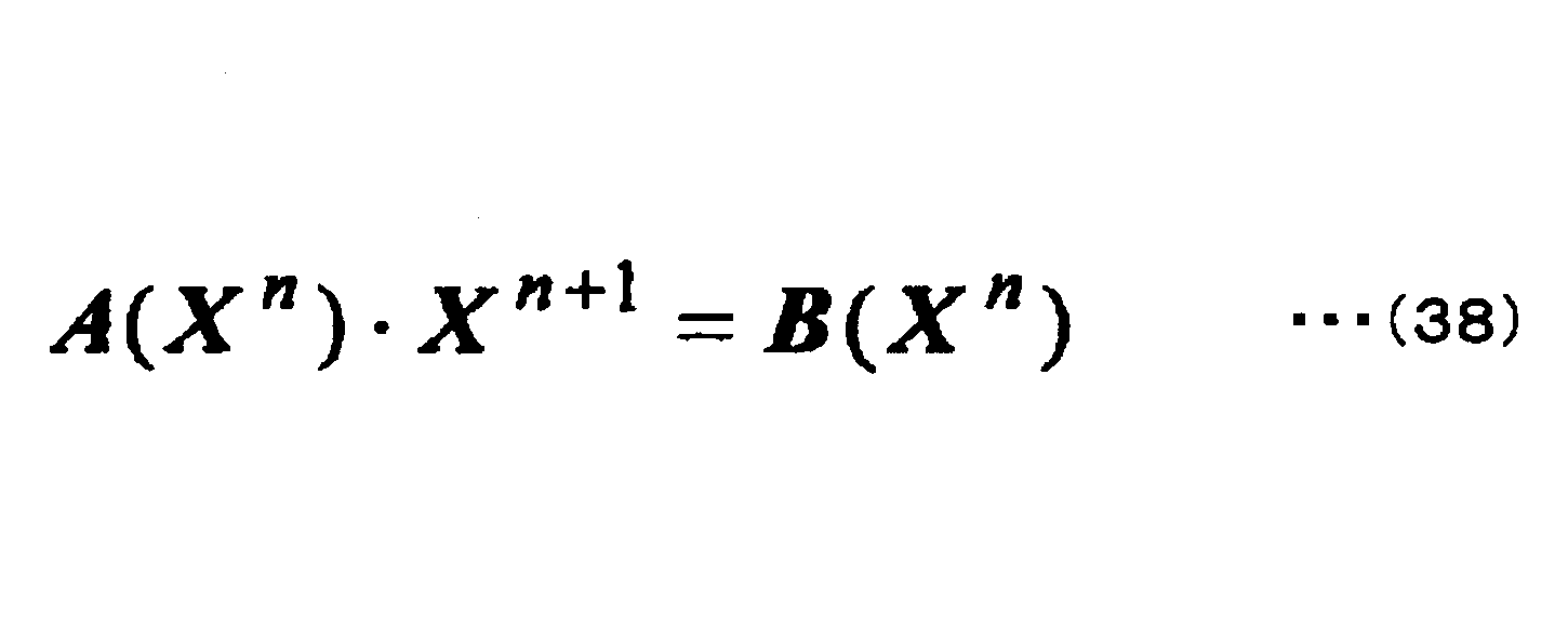
より詳細には、ポスト処理プログラムP3は、本実施形態の数値解析装置Aに対して、計算結果の可視化処理、抽出処理を実行させる。
ここで、可視化処理とは、例えば、断面コンター表示、ベクトル表示、等値面表示、アニメーション表示を出力装置5に出力させる処理である。また、抽出処理とは、作業者が指定する領域の定量値を抽出して数値やグラフとして出力装置5に出力させる、あるいは作業者が指定する領域の定量値を抽出してファイル化したものの出力を実行させる処理である。
また、ポスト処理プログラムP3は、本実施形態の数値解析装置Aに対して、自動レポート作成、計算残差の表示及び分析を実行させる。
データ記憶部2bは、図17に示すように、第一計算用データモデルM1、第二計算用データモデルM2、境界条件を示す境界条件データD1、計算条件を示す計算条件データD2、物性値を示す物性値データD3、及び初期条件を示す初期条件データD4を有するソルバ入力データファイルFと、3次元形状データD5と、計算結果データD6等を記憶するものである。また、データ記憶部2bは、CPU1の処理過程において生成される中間データを一時的に記憶する。
DVDドライブ3は、DVDメディアXを取り込み可能に構成されており、CPU1から入力される指令に基づいて、DVDメディアXに記憶されるデータを出力するものである。そして、本実施形態においては、DVDメディアXに数値解析プログラムPが記憶されており、DVDドライブ3は、CPU1から入力される指令に基づいて、DVDメディアXに記憶される数値解析プログラムPを出力する。
入力装置4は、本実施形態の数値解析装置Aと作業者とのマンマシンインターフェイスであり、ポインティングデバイスであるキーボード4aやマウス4bを備えている。
出力装置5は、CPU1から入力される信号を可視化して出力するものであり、ディスプレイ5a及びプリンタ5bを備えている。
通信装置6は、本実施形態の数値解析装置AとCAD装置C等の外部装置との間においてデータの受け渡しを行い、社内LAN(Local Area Network)等のネットワークBに対して電気的に接続されている。
次に、このように構成された本実施形態の数値解析装置Aを用いた数値解析方法(本実施形態の数値解析方法)について、図18~図20のフローチャートを参照して説明する。
図18のフローチャートに示すように、本実施形態の数値解析方法は、プリ処理(ステップS1)と、ソルバ処理(ステップS2)と、ポスト処理(ステップS3)とから構成されている。
なお、本実施形態の数値解析方法を行うより前に、CPU1は、DVDドライブ3に取り込まれたDVDメディアXに記憶された数値解析プログラムPをDVDメディアXから取り出し、記憶装置2のプログラム記憶部2aに記憶させる。
そして、CPU1は、入力装置4から数値解析の開始を指示する信号が入力されると、記憶装置2に記憶された数値解析プログラムPに基づいて数値解析を実行する。より詳細には、CPU1は、プログラム記憶部2aに記憶されたプリ処理プログラムP1に基づいてプリ処理(ステップS1)を実行し、プログラム記憶部2aに記憶されたソルバ処理プログラムP2に基づいてソルバ処理(ステップS2)を実行し、プログラム記憶部2aに記憶されたポスト処理プログラムP3に基づいてポスト処理(ステップS3)を実行する。なお、このようにCPU1がプリ処理プログラムP1に基づくプリ処理(ステップS1)を実行することによって、本実施形態の数値解析装置Aが計算用データモデル作成部として機能される。また、CPU1がソルバ処理プログラムP2に基づくソルバ処理(ステップS2)を実行することによって、本実施形態の数値解析装置Aが物理量計算部として機能される。
図19は、プリ処理(ステップS1)を示すフローチャートである。この図に示すように、プリ処理(ステップS1)が開始されると、CPU1は、通信装置6に、ネットワークBを介してCAD装置Cから自動車のキャビン空間を含む3次元形状データD5を取得させる(ステップS1a)。CPU1は、取得した3次元形状データD5を記憶装置2のデータ記憶部2bに記憶させる。
続いて、CPU1は、ステップS1aで取得した3次元形状データD5に基づいて、第一計算用データモデルの作成を実行する(ステップS1b)。
具体的には、CPU1は、キャビン空間を示す解析領域に含まれる各分割領域内に1つのコントロールポイントを仮想的に配置する。ここでは、CPU1は、分割領域の重心を算出し、各々の重心に対して1つのコントロールポイントを仮想的に配置する。そして、CPU1は、コントロールポイントの配置情報、各コントロールポイントが占めるコントロールボリュームの体積(コントロールポイントが配置される分割領域の体積)を算出し、記憶装置2のデータ記憶部2bに一時的に記憶させる。
また、CPU1は、分割領域同士の境界面である境界面の面積及び第一法線ベクトルを算出し、これらの境界面の面積及び第一法線ベクトルを記憶装置2のデータ記憶部2bに一時的に記憶させる。
また、CPU1は、分割領域間のlinkを作成し、この分割領域間のlinkを記憶装置2のデータ記憶部2bに一時的に記憶させる。
そして、CPU1は、データ記憶部2bに記憶された、コントロールポイントの配置情報と、各コントロールポイントが占めるコントロールボリュームの体積と、境界面の面積及び法線ベクトルと、linkとをデータベース化することによって第一計算用データモデルを作成し、作成した第一計算用データモデルを記憶装置2のデータ記憶部2b内に記憶させる。
また、本実施形態では、ステップS1bにおいて、先に分割領域を形成し、その後コントロールポイントを配置し、各コントロールポイントに対して、自らが配置された分割領域の体積を割り当てる構成を採用している。
しかしながら、本実施形態においては、先にコントロールポイントを解析領域に配置し、各コントロールポイントに対して後から体積を割り当てることも可能である。
具体的には、例えば、異なるコントロールポイントにぶつかるまでの半径や、結合関係にある(linkで関連付けられた)コントロールポイントまでの距離に基づいて、各コントロールポイントに対して重み付けを行う。
ここでコントロールポイントiの重みをwi、基準体積をV+とし、コントロールポイントiに割り当てられる体積Viを下式(39)とする。

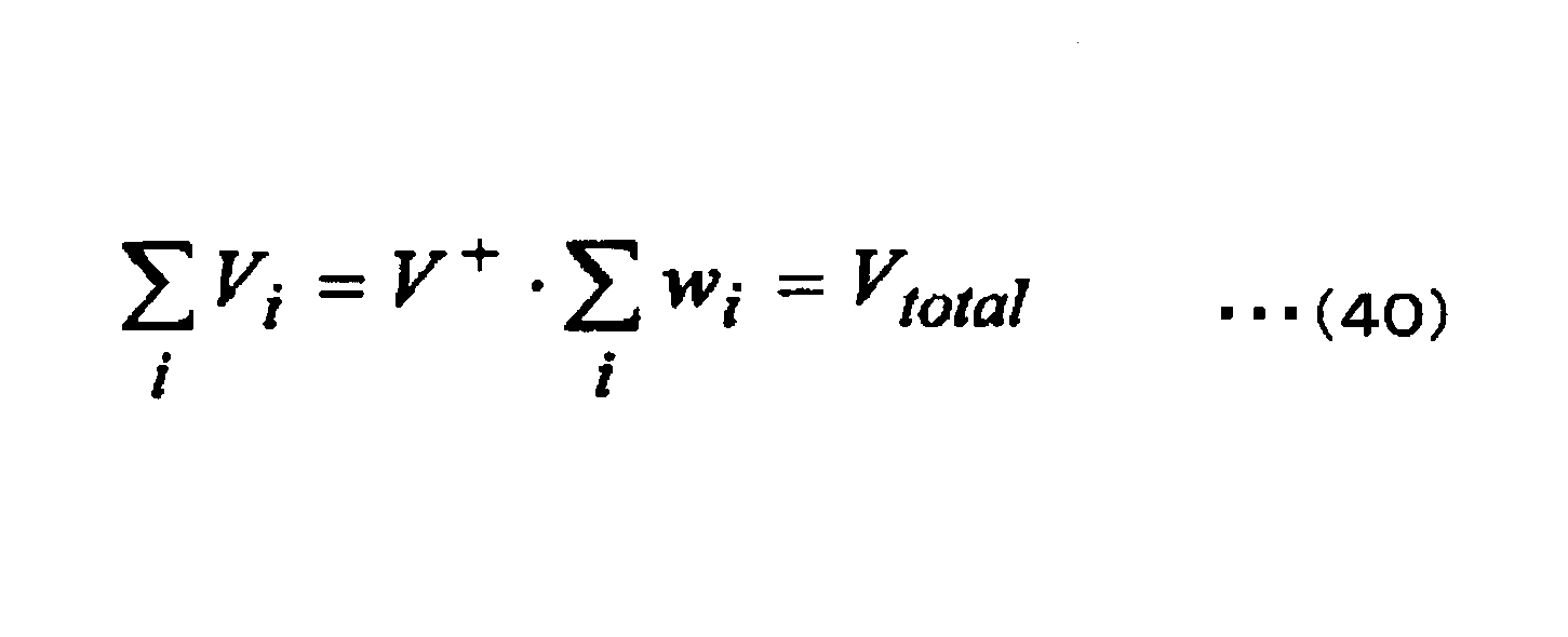

このような方法を用いれば、プリ処理において、幾何学的形状を規定する量を用いることなく、第一計算用データモデルに持たせる分割領域の体積を求めることができる。
また、当該第一計算用データモデルの作成(ステップS1b)において、CPU1は、GUIを形成し、GUIから指令(例えば分割領域の密度を示す指令や分割領域の形状を示す指令)が入力された場合には、当該指令を反映させた処理を実行する。したがって、作業者は、GUIを操作することによって、コントロールポイントの配置や分割領域の形状を任意に調節することが可能とされている。
ただし、CPU1は、数値解析プログラムに記憶された保存則を満足するための3つの条件に照らし合わせ、GUIから入力される指令が、当該条件から外れる場合には、その旨をディスプレイ5aに表示させる。
続いて、CPU1は、ステップS1bで作成した第一計算用データモデルに基づいて、第二計算用データモデルの作成を実行する(ステップS1c)。
具体的には、CPU1は、作成された第一計算用データモデルを用いて、図7あるいは図8に示す方法でコントロールボリューム(セル)を集合させ、キャビン空間を示す解析領域内に、集合領域を生成する。次に、CPU1は、キャビン空間を示す解析領域に含まれる各集合領域内に1つの集合コントロールポイントを仮想的に配置する。ここでは、CPU1は、第一計算用データモデルに基づいて、式(20)及び(21)によって、集合コントロールポイントを算出し、各々の集合領域に対して1つの集合コントロールポイントを仮想的に配置する。そして、CPU1は、集合コントロールポイントの配置情報、各集合コントロールポイントが占める集合コントロールボリュームの体積(集合コントロールポイントが配置される集合領域の体積)を算出し、記憶装置2のデータ記憶部2bに一時的に記憶させる。
また、CPU1は、集合領域同士の境界面である境界面の面積及び第二法線ベクトルを算出し、これらの境界面の面積及び第二法線ベクトルを記憶装置2のデータ記憶部2bに一時的に記憶させる。
また、CPU1は、集合領域のlinkを作成し、この集合領域のlinkを記憶装置2のデータ記憶部2bに一時的に記憶させる。
そして、CPU1は、データ記憶部2bに記憶された、集合コントロールポイントの配置情報と、各集合コントロールポイントを有する集合領域の体積と、境界面の面積及び第二法線ベクトルと、linkとをデータベース化することによって第二計算用データモデルを作成し、作成した第二計算用データモデルを記憶装置2のデータ記憶部2b内に記憶させる。
また、当該第二計算用データモデルの作成(ステップS1c)において、CPU1は、GUIを形成し、GUIから指令(例えば分割領域の密度を示す指令や分割領域の形状を示す指令)が入力された場合には、当該指令を反映させた処理を実行する。したがって、作業者は、GUIを操作することによって、集合コントロールポイントの配置や集合領域の形状を任意に調節することが可能とされている。なお、集合領域は、あくまでもコントロールボリューム(セル)の集合なので、集合領域に対してコントロールボリューム(セル)を無視して形状変更はできない。
ただし、CPU1は、数値解析プログラムに記憶された保存則を満足するための3つの条件に照らし合わせ、GUIから入力される指令が、当該条件から外れる場合には、その旨をディスプレイ5aに表示させる。
続いて、CPU1は、物性値データの設定(ステップS1d)を行う。具体的には、CPU1は、GUIを用いて、ディスプレイ5a上に物性値の入力画面を表示し、キーボード4aあるいはマウス4bから入力される物性値を示す信号を物性値データD3としてデータ記憶部2bに一時的に記憶させることで物性値の設定を行う。なお、ここで言う物性値とは、キャビン空間における流体である空気の特性値であり、空気の密度、粘性係数等である。
続いて、CPU1は、境界条件データの設定(ステップS1e)を行う。具体的には、CPU1は、GUIを用いて、ディスプレイ5a上に境界条件の入力画面を表示し、キーボード4aあるいはマウス4bから入力される境界条件を示す信号を境界条件データD1としてデータ記憶部2bに一時的に記憶させることで境界条件データの設定を行う。なお、ここで言う境界条件とは、キャビン空間の物理現象を支配する離散化支配方程式や、キャビン空間と外部空間との境界面に臨む集合コントロールポイントの特定情報、及びキャビン空間と外部空間との間における熱の伝熱条件等を示す。
なお、本実施形態の数値解析方法は、キャビン空間における流速を数値解析により求めることを目的とするため、上記離散化支配方程式として、前述のナビエ・ストークスの式に基づく離散化支配方程式(29)及び連続の式に基づく離散化支配方程式(30)が用いられる。
なお、これらの離散化支配方程式は、例えば、数値解析プログラムPに予め記憶された複数の離散化支配方程式をディスプレイ5a上に表示された複数の離散化支配方程式から作業者がキーボード4aやマウス4bを用いることによって選択される。
続いて、CPU1は、初期条件データの設定(ステップS1f)を行う。具体的には、CPU1は、GUIを用いて、ディスプレイ5a上に初期条件の入力画面を表示し、キーボード4aあるいはマウス4bから入力される初期条件を示す信号を初期条件データD4としてデータ記憶部2bに一時的に記憶させることで初期条件データの設定を行う。なお、ここ言う初期条件とは、各コントロールポイント(各分割領域)における初期流速、及び各集合コントロールポイント(各集合領域)における初期流速である。
続いて、CPU1は、計算条件データの設定(ステップS1g)を行う。具体的には、CPU1は、GUIを用いて、ディスプレイ5a上に計算条件の入力画面を表示し、キーボード4aあるいはマウス4bから入力される計算条件を示す信号を計算条件データD2としてデータ記憶部2bに一時的に記憶させることで計算条件データの設定を行う。なお、ここで言う計算条件とは、ソルバ処理(ステップS2)における計算の条件であり、例えば、反復回数や収束基準を示す。
続いて、CPU1は、ソルバ入力データファイルFの作成(ステップS1h)を行う。
具体的には、CPU1は、ステップS1bにて作成された第一計算用データモデルM1と、ステップS1cにて作成された第二計算用データモデルM2と、ステップS1dで設定された物性値データD3と、ステップS1eで設定された境界条件データD1と、ステップS1fで設定された初期条件データD4と、ステップS1gで設定された計算条件データD2とをソルバ入力データファイルFに格納することによってソルバ入力データファイルFを作成する。なお、このソルバ入力データファイルFは、データ記憶部2bに記憶される。
以上のようなプリ処理(ステップS1)が完了すると、CPU1は、ソルバ処理プログラムP2に基づいて、図18のフローチャートに示すソルバ処理(ステップS2)を実行する。
図20に示すように、ソルバ処理(ステップS2)が開始されると、CPU1は、プリ処理(ステップS1)で作成されたソルバ入力データファイルFを取得する(ステップS2a)。なお、本実施形態に示す数値解析方法のように、単一の装置(本実施形態の数値解析装置A)によってプリ処理及びソルバ処理を実行する場合には、既にデータ記憶部2bにソルバ入力データファイルFが記憶されているため、ステップS2aを省略することができる。ただし、プリ処理(ステップS1)とソルバ処理(ステップS2)とが異なる装置において実行される場合には、ネットワークやリムーバルディスクによって搬送されるソルバ入力データファイルFを取得する必要があるため、本ステップS2aを行う必要がある。
続いて、CPU1は、ソルバ入力データの整合性を判定する(ステップS2b)。なお、ソルバ入力データとは、ソルバ入力データファイルFに格納されたデータを示し、第一計算用データモデルM1、第二計算用データモデルM2、境界条件データD1、計算条件データD2、物性値データD3及び初期条件データD4である。
具体的には、CPU1は、ソルバ処理において物理量計算を実行可能なソルバ入力データがソルバ入力データファイルFに全て格納されているかを分析することによってソルバ入力データの整合性の判定を行う。
そして、CPU1は、ソルバ入力データが不整合であると判定した場合には、ディスプレイ5aにエラーを表示させ(ステップS2b+)、さらには不整合である部分のデータを入力するための画面を表示させる。その後、CPU1は、GUIから入力される信号に基づいてソルバ入力データの調整を行い(ステップS2c)、再度ステップS2aを実行する。
一方、CPU1は、ステップS2bにおいてソルバ入力データの整合性があると判定した場合には、初期計算処理(ステップS2e)を実行する。
具体的には、CPU1は、境界条件データD1に記憶された離散化支配方程式から離散化係数行列を作成し、さらにマトリクス計算用のデータテーブルの作成を行うことによって初期計算処理を行う。なお、境界条件データD1に記憶された離散化支配方程式とは、例えば、ナビエ・ストークスの式に基づく離散化支配方程式(29)及び連続の式に基づく離散化支配方程式(30)である。
なお、分割領域から作成される第一計算用データモデルをソルバ入力データとする数値計算を実行する場合は、CPU1は、境界条件データD1に記憶された離散化支配方程式から離散化係数行列を作成し、さらにマトリクス計算用のデータテーブルの作成を行うことによって初期計算処理を行う。なお、境界条件データD1に記憶された離散化支配方程式とは、例えば、ナビエ・ストークスの式に基づく離散化支配方程式(10)及び連続の式に基づく離散化支配方程式(11)である。
続いて、CPU1は、大規模疎行列方程式の組み上げ(ステップS2f)を行う。具体的には、CPU1は、ナビエ・ストークスの式に基づく離散化支配方程式(29)及び連続の式に基づく離散化支配方程式(30)から、前述の式(37)で示すマトリックス計算用の大規模疎行列方程式の組み上げを行う。
なお、分割領域から作成される第一計算用データモデルをソルバ入力データとする数値計算を実行する場合は、CPU1は、ナビエ・ストークスの式に基づく離散化支配方程式(10)及び連続の式に基づく離散化支配方程式(11)から、前述の式(37)で示すマトリックス計算用の大規模疎行列方程式の組み上げを行う。
続いて、CPU1は、離散化支配方程式に、非圧縮性や接触等の付帯条件が存在するかの判定を行う。この付帯条件は、例えば、境界条件データとしてソルバ入力データファイルFに格納されている。
そして、CPU1は、離散化支配方程式に付帯条件が存在すると判定した場合には当該付帯条件の大規模行列方程式の組み込み(ステップS2h)を実行した後に大規模行列方程式の計算(ステップS2i)を実行する。一方、CPU1は、離散化支配方程式に付帯条件が存在しないと判定した場合には付帯条件の大規模行列方程式の組み込み(ステップS2h)を実行することなく大規模行列方程式の計算(ステップS2i)を実行する。
そしてCPU1は、大規模行列方程式を例えば、CG法(共役勾配法)によって解き、前述の式(38)を用いて解のアップデート(ステップS2j)を行う。
続いて、CPU1は、式(38)の残差が収束条件に達したか否かの判定(ステップS2k)を行う。具体的には、CPU1は、式(38)の残差を計算し、計算条件データD2に含まれる収束条件と比較し、これによって式(38)の残差が収束条件に達したか否かの判定を行う。
そして、残差が収束条件に達していないと判定した場合には、CPU1は、物性値のアップデートを行った後、再度ステップS2gを実行する。つまり、CPU1は、式(38)の残差が収束条件に達するまで、物性値のアップデートを行いながらステップS2f~S2kを繰り返し行う。
一方、残差が収束条件に達したと判定した場合には、CPU1は、計算結果の取得を行う(ステップS2l)。具体的には、CPU1は、直前のステップS2iにおいて計算された物理量の解を計算結果データとしてデータ記憶部2bに記憶させることによって計算結果の取得を行う。
このようなソルバ処理(ステップS2)によって、キャビン空間における空気の流速が求められる。なお、このようなソルバ処理(ステップS2)は、本実施形態の物理量計算方法に相当する。
以上のようなソルバ処理(ステップS2)が完了すると、CPU1は、ポスト処理プログラムP3に基づいてポスト処理(ステップS3)を実行する。
具体的には、例えばCPU1は、GUIから入力される指令に基づいて、計算結果データから、例えば断面コンタデータ、ベクトルデータ、等値面データ、アニメーションデータを生成し、当該データを、出力装置5に可視化させる。
また、CPU1は、GUIから入力される指令に基づいて、キャビン空間の一部における定量値(計算結果)を抽出して数値やグラフとし、この数値やグラフを出力装置5に可視化させ、さらには数値やグラフをファイルとして纏めて出力する。また、CPU1は、GUIから入力される指令に基づいて、例えば計算結果データから自動レポート作成、計算残差の表示及び分析を行ってその結果を出力する。
さらに、本実施形態の数値解析装置A、数値解析方法及び数値解析プログラムの利用者が、ポスト処理の結果に応じて3次元形状データを変更して再度、図18のフローチャートの処理を繰り返す場合にも、現実的な時間内で物理量の計算が可能となる。
即ち、利用者は、ポスト処理により得られた計算結果データを評価することにより、解析対象である3次元形状データにより所望の結果が得られたと判断する場合には、シミュレーションを終了してよい。また利用者は、ポスト処理により得られた計算結果データを評価することにより、解析対象である3次元形状データにより所望の結果が得られていないと判断する場合には、3次元形状データを修正してから再度シミュレーションを実行してよい。
上記の動作において、シミュレーションが所望の結果を示す場合、その解析対象であった3次元形状データが表現する物理的実体(閉鎖された空間を構成する自動車キャビン、コックピット、住宅、若しくは電気機器や産業機器の内部等、又はガラスや鉄鋼等の製造装置等)の設計が満足できるものと判断し、当該物理的実体を製造・生産してよい。またシミュレーションが所望の結果を示さない場合、その解析対象で、あった3次元形状データが表現する物理的実体の設計が満足できないものと判断し、当該物理的実体の設計を変更し、この設計変更後の3次元形状データに基づいて再度シミュレーションを実行することになる。
以上のような本実施形態の数値解析装置A、数値解析方法及び数値解析プログラムによれば、プリ処理にて集合コントロールボリュームの体積と境界面の面積及び第二法線ベクトルとを有する第二計算用データモデルM2が作成され、ソルバ処理にて第二計算用データモデルM2に含まれる集合コントロールボリュームの体積と境界面の面積及び第二法線ベクトルとを用いて各集合コントロールボリュームにおける物理量が計算される。
このように、本実施形態の数値解析方法を用いることで、物理量を計算することができる。そのため、本実施形態の数値解析方法は、物理現象を数値的に解析する物理現象解析方法である。
なお、本実施形態の数値解析装置A、数値解析方法及び数値解析プログラムにおいては、解析領域に分割領域を重なることなく充填させている。このため、前述した保存側を満足するための6つの条件(a1)~(c1)及び(a2)~(c2)が満たされることとなり、保存則を満足して流速を計算することができる。
このように構成された本実施形態の数値解析装置Aは、幾何学的形状を規定する量を有さない計算用データモデルであって、保存則を満たす計算用データモデルを作成するため、解析領域の分割数を少なくしてソルバ処理における計算負荷を軽くすることと、解析領域の分割数を少なくしても解析精度を悪くしないこととを両立することが可能である。
また、本実施形態の数値解析装置A、数値解析方法及び数値解析プログラムによれば、前述のように、プリ処理における第一及び第二計算用データモデルの作業負担が大幅に減少し、またソルバ処理における計算負荷を軽減させることが可能となる。
したがって、解析領域が移動境界を含み解析領域の形状が時系列的に変化する場合であっても、本実施形態によれば、図21のフローチャートに示すように、解析領域が形状変化するたびにプリ処理とソルバ処理とを繰り返し行うことによって、現実的な時間内で物理量の計算が可能となる。 さらに、本実施形態の数値解析装置A、数値解析方法及び数値解析プログラムの利用者が、ポスト処理の結果に応じて3次元形状データを変更して再度、図21のフローチャートの処理を繰り返す場合にも、現実的な時間内で物理量の計算が可能となる。
即ち、利用者は、ポスト処理により得られた計算結果データを評価することにより、解析対象である3次元形状データにより所望の結果が得られたと判断する場合には、シミュレーションを終了してよい。また利用者は、ポスト処理により得られた計算結果データを評価することにより、解析対象である3次元形状データにより所望の結果が得られていないと判断する場合には、3次元形状データを修正してから再度シミュレーションを実行してよい。
上記の動作において、シミュレーションが所望の結果を示す場合、その解析対象であった3次元形状データが表現する物理的実体(閉鎖された空間を構成する自動車キャビン、コックピット、住宅、若しくは電気機器や産業機器の内部等、又はガラスや鉄鋼等の製造装置等)の設計が満足できるものと判断し、当該物理的実体を製造・生産してよい。またシミュレーションが所望の結果を示さない場合、その解析対象で、あった3次元形状データが表現する物理的実体の設計が満足できないものと判断し、当該物理的実体の設計を変更し、この設計変更後の3次元形状データに基づいて再度シミュレーションを実行することになる。
移動境界は、解析領域の中で、対象とする物体が移動することによって変化する物体の境界をいう。解析領域が移動境界を含み解析領域の形状が時系列的に変化する場合としては、例えば、キャビンにおいて、人がいない状態から、人がキャビン内に入るまでの現象を再現する場合が挙げられる。その他、例えば、加熱炉の中を加熱対象物が移動する現象を再現する場合が挙げられる。
以上、添付図面を参照しながら本実施形態の好適な実施形態について説明したが、本実施形態は、上記実施形態に限定されないことは言うまでもない。前述した実施形態において示した各構成部材の諸形状や組み合わせ等は一例であって、本実施形態の主旨から逸脱しない範囲において設計要求等に基づき種々変更可能である。
上記実施形態においては、運動量保存の方程式の変形例であるナビエ・ストークスの式及び連続の式から導出した離散化支配方程式を用いて空気の流速を数値解析によって求める構成について説明した。
しかしながら、本実施形態はこれに限定されるものではなく、質量保存の方程式、運動量保存の方程式、角運動量保存の方程式、エネルギ保存の方程式、移流拡散方程式及び波動方程式の少なくともいずれかから導出した離散化支配方程式を用いて物理量を数値解析によって求めることが可能である。
また、上記実施形態においては、本実施形態の境界面特性量として、境界面の面積と境界面の法線ベクトルとを用いる構成について説明した。
しかしながら、本実施形態はこれに限定されるものではなく、境界面特性量として他の量(例えば境界面の周長)を用いることもできる。
また、上記実施形態においては、保存則を満足するために前述の6つの条件を満たすように計算用データモデルを作成する構成について説明した。
しかしながら、本実施形態はこれに限定されるものではなく、保存則を満足させる必要がない場合には、計算用データモデルを必ずしも前述の6つの条件を満たすように作成する必要はない。
また、上記実施形態においては、分割領域の体積を、当該分割領域の内部に配置されるコントロールポイントが占めるコントロールボリュームの体積として捉えた構成について説明した。
しかしながら、本実施形態はこれに限定されるものではなく、分割領域の内部に対してコントロールポイントを配置する必要は必ずしもない。このような場合には、コントロールポイントが占めるコントロールボリュームの体積を分割領域の体積に置き換えることによって数値解析を行うことができる。
また、上記実施形態においては、解析領域をまずは複数のコントロールボリューム(セル)に分割して第一計算用データモデルを作成し、次に、コントロールボリューム(セル)を集合させた集合領域(ドメイン)によって解析領域を分割して第二計算用データモデルを作成した。そして、そのソルバ処理においては、第二計算用データモデルを用いて計算を行った。しかし、第二計算用データモデルは、セルを集合させたドメインに基づく計算用データモデルであればよく、セルを集合させたドメインをさらに集合させた新たなドメインでの計算用データモデルであってもよい。
図22~図38は、本実施形態における第一計算用データモデル(分割領域)及び第二計算用データモデル(集合領域)を使用して実施した熱流体シミュレーション結果の一例を示す図である。
本実施形態では、流体解析の基礎方程式として、式(1)で示すナビエ・ストークスの式と、式(2)で示す連続の式を用いた数値計算方法を説明したが、前述の通り、本実施形態では、ナビエ・ストークスの式だけでなく、移流拡散方程式に対しても重み付き残差積分法に基づいて、幾何学的形状を規定する量を必要としない量のみを使用する離散化支配方程式が導出可能であることを説明した。図22~図38に示す熱流体シミュレーションの実行では、熱流体解析の基礎方程式として、式(1)で示すナビエ・ストークスの式と、式(2)で示す連続の式に加え、熱の移流拡散方程式を基礎方程式として使用した。熱の移流拡散方程式に対する本実施形態での重み付き残差積分法に基づく幾何学的形状を規定する量を必要としない量のみを使用する離散化支配方程式の導出については、特許文献1に詳細が記載されているためここでは説明を省略する。
熱流体シミュレーションでは、解析領域の一例は自動車のキャビンであり、境界条件の一例は夏季で、冷房空調条件である。具体的には、車外参照温度は35度、車外熱伝達率は40W/m2K、乗車人員数は4名、空調吹出風速は5m/s、空調吹出温度は8℃である。なお、必要に応じて、境界条件として、エンジンルームの温度、トランクルームの温度、床下フロアーの温度、ダッシュボードの内側の温度、天井の温度、その他の少なくとも一つが含まれる場合等も解析可能である。
数値解析装置Aは、解析領域(自動車のキャビン)を、前述したように、頂点の座標(Vertex)及び該頂点の連結情報(Connectivity)を必要としないセルに分割する。
解析領域(自動車のキャビン)を、約450万個のセルに分割した第一計算用データモデルを使用して実施した3D熱流体シミュレーション結果の一例を、図22~図24に示す。図22は、解析領域であるキャビン空間内の運転席中央での垂直断面上の温度コンター図であり、図23は、その垂直断面上の7点のサンプリング点での温度値(以降、温度値の単位はK(ケルビン)で表示する。)を示す。また、図24は、解析領域であるキャビン空間内の運転席中央での垂直断面上の流速コンター図であり、流速の向きを矢印の向き、流速の大きさを矢印の大きさで示す。図22~図24に示す結果は、定常状態の計算結果を得るまでに、インテル社製CPU Xeon(2.6GHz)を搭載したPCを用いて、約30時間の計算時間を要した。
本実施形態では、数値解析装置Aは、解析領域(自動車のキャビン)に対して約450万個のセルを自動生成する。数値解析装置Aは、前述したセルから集合領域を生成する処理によって、図25~図32に示す約450万個のセルから27個の集合領域(ドメイン)を生成する場合について説明する。27個の集合領域の各々を生成した結果の一例を、図25~図30に示す。図25~図30の各々において、DCPは集合領域(ドメイン)のコントロールポイントであり、CCPはセルのコントロールポイントの一つである。図25~図30は、順番にドメイン1からドメイン6までを示す。また、図25~図30には、図示されていないが、数値解析装置Aは、各集合領域について、外表面を取得する。数値解析装置Aは、取得した外表面と、その外表面に接している部材との間の境界条件を取得する。境界条件は、外表面が接する部材の材料によって異なる場合がある。
図31と図32は、前述の27個の集合領域(ドメイン)を含む第二計算用データモデルを使用して実施した3D熱流体シミュレーション結果の一例を示す。
図31は、解析領域であるキャビン空間内の運転席中央での垂直断面上の温度コンター図であり、その垂直断面上の7点のサンプリング点での温度値を示す。図31の7点のサンプリング点での温度値は、それぞれ上段の温度値と下段の括弧内の温度値に分けて示しているが、上段は前述の27個の集合領域(ドメイン)を含む第二計算用データモデルを使用して実施した3D熱流体シミュレーション結果の温度値であり、下段の括弧内の温度値は図23に示す約450万個の分割領域(セル)に分割した第一計算用データモデルを使用して実施した3D熱流体シミュレーション結果の温度値を示す。上段と下段の温度値を比較すると、数度の温度値の差はあるものの平均的には良く一致している。
図32は、解析領域であるキャビン空間内の運転席中央での垂直断面上の温度コンター図であり、その同じ垂直断面上に流速ベクトルを重ねて示した図である。キャビン空間内に空調吹出流れによる循環流が形成されていることが分かるが、図24に示す約450万個のセルに分割した第一計算用データモデルを使用して実施した3D熱流体シミュレーション結果と比較すると、図32ではキャビン空間内の流れの詳細な分布までは計算できていないことが分かる。
図31と図32に示す27個の集合領域(ドメイン)を含む第二計算用データモデルを使用して実施した3D熱流体シミュレーションは、定常状態の計算結果を得るまでに、インテル社製CPU Xeon(2.6GHz)を搭載したPCを用いて、1秒以下の計算時間を要した。約450万個のセルに分割した第一計算用データモデルを使用して実施した3D熱流体シミュレーションに約30時間の計算時間を要したことと比較すると数値計算は非常に高速である。
図33と図34は、792個の集合領域(ドメイン)を含む第二計算用データモデルを使用して実施した3D熱流体シミュレーション結果の一例を示す。
図33は、解析領域であるキャビン空間内の運転席中央での垂直断面上の温度コンター図であり、その垂直断面上の7点のサンプリング点での温度値を示す。図31と同様に、7点のサンプリング点での温度値は、それぞれ上段の温度値と下段の括弧内の温度値に分けて示しているが、上段は792個の集合領域(ドメイン)を含む第二計算用データモデルを使用して実施した3D熱流体シミュレーション結果の温度値であり、下段の括弧内の温度値は図35に示す約450万個のセルに分割した第一計算用データモデルを使用して実施した3D熱流体シミュレーション結果の温度値を示す。上段と下段の温度値を比較すると、数度の温度値の差はあるものの平均的には良く一致している。
図34は、解析領域であるキャビン空間内の運転席中央での垂直断面上の温度コンター図であり、その同じ垂直断面上に流速ベクトルを重ねて示した図である。キャビン空間内に空調吹出流れによる循環流が形成されていることが分かるが、図32と比較すると、図34ではキャビン空間内の流れの詳細度が向上していることが分かる。
図33と図34に示す792個の集合領域(ドメイン)を含む第二計算用データモデルを使用して実施した3D熱流体シミュレーションは、定常状態の計算結果を得るまでに、インテル社製CPU Xeon(2.6GHz)を搭載したPCを用いて、約20秒の計算時間を要した。約450万個のセルに分割した第一計算用データモデルを使用して実施した3D熱流体シミュレーションに約30時間の計算時間を要したことと比較すると数値計算は非常に高速である。
図35と図36は、16055個の集合領域を含む第二計算用データモデルを使用して実施した3D熱流体シミュレーション結果の一例を示す。
図35は、解析領域であるキャビン空間内の運転席中央での垂直断面上の温度コンター図であり、その垂直断面上の7点のサンプリング点での温度値を示す。図31と同様に、7点のサンプリング点での温度値は、それぞれ上段の温度値と下段の括弧内の温度値に分けて示しているが、上段は16055個の集合領域(ドメイン)を含む第二計算用データモデルを使用して実施した3D熱流体シミュレーション結果の温度値であり、下段の括弧内の温度値は図35に示す約450万個のセルに分割した第一計算用データモデルを使用して実施した3D熱流体シミュレーション結果の温度値を示す。上段と下段の温度値を比較すると、温度値の差は1度程度であり非常に良く一致している。
図36は、解析領域であるキャビン空間内の運転席中央での垂直断面上の温度コンター図であり、その同じ垂直断面上に流速ベクトルを重ねて示した図である。キャビン空間内に空調吹出流れによる循環流が形成されていることが分かるが、図32、図34と比較すると、図36ではキャビン空間内の流れの詳細度が大きく向上しており、キャビン空間内の局所的な流れや渦も計算できていることが分かる。
図35と図36に示す16055個の集合領域(ドメイン)を含む第二計算用データモデルを使用して実施した3D熱流体シミュレーションは、定常状態の計算結果を得るまでに、インテル社製CPU Xeon(2.6GHz)を搭載したPCを用いて、約3分の計算時間を要した。約450万個のセルに分割した第一計算用データモデルを使用して実施した3D熱流体シミュレーションに約30時間の計算時間を要したことと比較すると数値計算は非常に高速である。
図37と図38は、66257個の集合領域を含む第二計算用データモデルを使用して実施した3D熱流体シミュレーション結果の一例を示す。
図37は、解析領域であるキャビン空間内の運転席中央での垂直断面上の温度コンター図であり、その垂直断面上の7点のサンプリング点での温度値を示す。図31と同様に、7点のサンプリング点での温度値は、それぞれ上段の温度値と下段の括弧内の温度値に分けて示しているが、上段は66257個の集合領域(ドメイン)を含む第二計算用データモデルを使用して実施した3D熱流体シミュレーション結果の温度値であり、下段の括弧内の温度値は図23に示す約450万個のセルに分割した第一計算用データモデルを使用して実施した3D熱流体シミュレーション結果の温度値を示す。上段と下段の温度値を比較すると、温度値の差はゼロであり非常に良く一致している。
図38は、解析領域であるキャビン空間内の運転席中央での垂直断面上の温度コンター図であり、その同じ垂直断面上に流速ベクトルを重ねて示した図である。キャビン空間内に空調吹出流れによる循環流が形成されていることが分かるが、図32、図34と比較すると、図38ではキャビン空間内の流れの詳細度が大きく向上しており、キャビン空間内の局所的な流れや渦も計算できており、図24に示す約450万個のセルに分割した第一計算用データモデルを使用して実施した3D熱流体シミュレーション結果と比較しても精度上差異のない結果である。
図37と図38に示す66257個の集合領域(ドメイン)を含む第二計算用データモデルを使用して実施した3D熱流体シミュレーションは、定常状態の計算結果を得るまでに、インテル社製CPU Xeon(2.6GHz)を搭載したPCを用いて、約12分の計算時間を要した。約450万個のセルに分割した第一計算用データモデルを使用して実施した3D熱流体シミュレーションに約30時間の計算時間を要したことと比較すると数値計算は非常に高速である。
前述の通り、集合領域(ドメイン)の個数が、27個、792個、16055個、66257個の集合領域(ドメイン)を含む第二計算用データモデルを使用して実施した3D熱流体シミュレーション結果の一例を示した。また、約450万個のセルに分割した第一計算用データモデルを使用して実施した3D熱流体シミュレーション結果と比較して、第二計算用データモデルを使用して実施した3D熱流体シミュレーション結果の精度を示した。さらに、第二計算用データモデルを使用して実施した3D熱流体シミュレーションは、第一計算用データモデルを使用して実施した3D熱流体シミュレーションの計算速度と比較して、非常に高速であることを示した。解析する目的や必要とされる精度に応じて、集合領域(ドメイン)の数を適切に選択することによって、特許文献1に相当するセルのみを使用した計算に比べ非常に高速に解析結果を得ることができることを示した。
また、上記実施形態においては、数値解析プログラムPがDVDメディアXに記憶されて搬送可能な構成について説明した。
しかしながら、本実施形態はこれに限定されるものではなく、数値解析プログラムPを他のリムーバブルメディアに記憶させて搬送可能とする構成を採用することもできる。
また、プリ処理プログラムP1とソルバ処理プログラムP2とを別々のリムーバブルメディアに記憶させて搬送可能とすることもできる。また、数値解析プログラムPは、ネットワークを介して伝達することも可能である。
なお、本実施形態は、例えば、自動車ボディの形状、エアコンなどのHeating Ventilation and Air Conditioning(HVAC)での消費エネルギ、ガラス、人の存在、外部日射エネルギ、湿度、車速等をシミュレーションモデルに反映した自動車のキャビンの温熱解析に用いられてもよい。
また、本実施形態は、自動車のキャビンの温熱解析以外にも、自動車のエンジンの燃焼解析や、自動車の燃焼ガスの排気効率の解析や、自動車のエンジンルームの温熱解析等に用いられてもよい。
また、本実施形態は、自動車以外の分野における温熱解析に用いられてもよい。例えば、航空機、船舶、宇宙船、宇宙ステーションのキャビン、コックピット等の内部空間の温熱解析に用いられてもよい。また、例えば、住宅、ビル、アトリウム等の内部空間の温熱解析に用いられてもよい。また、例えば、電気機器や産業機器の内部の温熱解析に用いられてもよい。また、例えば、ガラス、鉄鋼等の製造設備の装置自体の温熱解析に用いられてもよいし、それら製造設備の装置周辺の温熱解析に用いられてもよい。
なお、第一計算用データモデルは、分割領域の計算用データモデルの一例である。また、第二計算用データモデルは、集合領域の計算用データモデルの一例である。また、分割領域の境界面特性量は、分割領域特性量の一例である。また、集合領域の境界面特性量は、集合領域特性量の一例である。また、第一法線ベクトルは、分割領域の境界面の法線ベクトルの一例である。また、第二法線ベクトルは、集合領域の境界面の法線ベクトルの一例である。なお、重み付き残差積分法に基づいて導出された離散化支配方程式と集合領域の体積と境界面特性量とによって算出された物理量と、空気の流速とは、解析結果である物理量の一例である。なお、数値解析方法はシミュレーション方法の一例である。
本出願を詳細にまた特定の実施態様を参照して説明したが、本発明の精神と範囲を逸脱することなく様々な変更や修正を加えることができることは当業者にとって明らかである。
上述した実施の形態に関し、さらに以下の付記を開示する。
(付記1)
コンピュータによって物理現象での物理量を数値的に解析するシミュレーション方法であって、コンピュータが、外部装置から解析領域の3次元形状データを取得し、
前記解析領域を複数の分割領域に分割し、
前記分割領域の頂点の座標(Vertex)及び該頂点の連結情報(Connectivity)を必要としない量のみを使用すると共に重み付き残差積分法に基づいて導出された離散化された分割領域での支配方程式に基づき、各前記分割領域の体積と隣り合う前記分割領域同士の特性を示す分割領域特性量とを前記分割領域の頂点の座標(Vertex)及び該頂点の連結情報(Connectivity)を必要としない量として有する前記分割領域での計算用データモデルを生成し、
前記分割領域を複数集合させることによって、要求される数の集合領域を生成し、
前記集合領域の頂点の座標(Vertex)及び該頂点の連結情報(Connectivity)を必要としない量のみを使用すると共に重み付き残差積分法に基づいて導出された離散化された集合領域での支配方程式に基づき、各前記集合領域の体積と隣り合う前記集合領域同士の特性を示す集合領域特性量とを前記集合領域の頂点の座標(Vertex)及び該頂点の連結情報(Connectivity)を必要としない量として有する前記集合領域での計算用データモデルを生成し、
前記解析領域での物性値と、前記集合領域での計算用データモデルとに基づいて、前記集合領域での解析結果である物理量を計算し、
前記解析結果である物理量の可視化データを生成して出力装置に表示し、
当該シミュレーション方法の利用者が、前記出力装置に表示された内容に応じて前記解析領域の前記形状を変更して再度、前記解析領域の前記形状変更後の3次元形状データから前記出力装置への表示までを繰り返すシミュレーション方法。
(付記2)
コンピュータによって物理現象での物理量を数値的に解析するシミュレーション方法であって、
コンピュータが、外部装置から解析領域の3次元形状データを取得して前記解析領域を複数の分割領域に分割し、
前記分割領域の頂点の座標(Vertex)及び該頂点の連結情報(Connectivity)を必要としない量のみを使用すると共に重み付き残差積分法に基づいて導出された離散化された分割領域での支配方程式に基づき、各前記分割領域の体積と隣り合う前記分割領域同士の特性を示す分割領域特性量とを前記分割領域の頂点の座標(Vertex)及び該頂点の連結情報(Connectivity)を必要としない量として有する前記分割領域での計算用データモデルを生成し、
前記分割領域を複数集合させることによって、要求される数の集合領域を生成し、
前記集合領域の頂点の座標(Vertex)及び該頂点の連結情報(Connectivity)を必要としない量のみを使用すると共に重み付き残差積分法に基づいて導出された離散化された集合領域での支配方程式に基づき、各前記集合領域の体積と隣り合う前記集合領域同士の特性を示す集合領域特性量とを前記集合領域の頂点の座標(Vertex)及び該頂点の連結情報(Connectivity)を必要としない量として有する前記集合領域での計算用データモデルを生成し、
前記解析領域での物性値と、前記集合領域での計算用データモデルとに基づいて、前記集合領域での解析結果である物理量を計算し、
前記解析領域が移動境界を含む場合には、前記解析領域の形状が時系列的に変化したかどうかを判断し、変化した場合には、前記前記分割領域での計算用データモデルの生成、前記集合領域での計算用データモデルの生成、前記集合領域での解析結果である物理量の計算を繰り返し、
変化しない場合には、前記解析結果である物理量の可視化データを生成して出力装置に表示する、シミュレーション方法。
(付記3)
コンピュータによって物理現象での物理量を数値的に解析するシミュレーション方法であって、
コンピュータが、外部装置から解析領域の3次元形状データを取得して前記解析領域を複数の分割領域に分割し、
前記分割領域の頂点の座標(Vertex)及び該頂点の連結情報(Connectivity)を必要としない量のみを使用すると共に重み付き残差積分法に基づいて導出された離散化された分割領域での支配方程式に基づき、各前記分割領域の体積と隣り合う前記分割領域同士の特性を示す分割領域特性量とを前記分割領域の頂点の座標(Vertex)及び該頂点の連結情報(Connectivity)を必要としない量として有する前記分割領域での計算用データモデルを生成し、
前記分割領域を複数集合させることによって、要求される数の集合領域を生成し、
前記集合領域の頂点の座標(Vertex)及び該頂点の連結情報(Connectivity)を必要としない量のみを使用すると共に重み付き残差積分法に基づいて導出された離散化された集合領域での支配方程式に基づき、各前記集合領域の体積と隣り合う前記集合領域同士の特性を示す集合領域特性量とを前記集合領域の頂点の座標(Vertex)及び該頂点の連結情報(Connectivity)を必要としない量として有する前記集合領域での計算用データモデルを生成し、
前記解析領域での物性値と、前記集合領域での計算用データモデルとに基づいて、前記集合領域での解析結果である物理量を計算し、前記解析結果である物理量の可視化データを生成して出力装置に表示する、シミュレーション方法。
(付記4)
前記分割領域での計算用データモデルの生成において、
全分割領域の体積の総和が解析領域の体積と一致するという条件と、
前記分割領域同士の境界面の面積が一致するという条件及び法線ベクトルが当該境界面を挟む一方の分割領域から見た場合と他方の分割領域から見た場合とで絶対値が一致するという条件と、
前記分割領域を通る無限に広い投影面Pの任意の向きの単位法線ベクトルが[n]p、境界面の面積がSi、境界面の単位法線ベクトルが[n]i、分割領域の面の総数がm、前記[]で囲まれた文字がベクトルを示す太字であるときに下式(1)が成り立つという条件と、
(付記1)
コンピュータによって物理現象での物理量を数値的に解析するシミュレーション方法であって、コンピュータが、外部装置から解析領域の3次元形状データを取得し、
前記解析領域を複数の分割領域に分割し、
前記分割領域の頂点の座標(Vertex)及び該頂点の連結情報(Connectivity)を必要としない量のみを使用すると共に重み付き残差積分法に基づいて導出された離散化された分割領域での支配方程式に基づき、各前記分割領域の体積と隣り合う前記分割領域同士の特性を示す分割領域特性量とを前記分割領域の頂点の座標(Vertex)及び該頂点の連結情報(Connectivity)を必要としない量として有する前記分割領域での計算用データモデルを生成し、
前記分割領域を複数集合させることによって、要求される数の集合領域を生成し、
前記集合領域の頂点の座標(Vertex)及び該頂点の連結情報(Connectivity)を必要としない量のみを使用すると共に重み付き残差積分法に基づいて導出された離散化された集合領域での支配方程式に基づき、各前記集合領域の体積と隣り合う前記集合領域同士の特性を示す集合領域特性量とを前記集合領域の頂点の座標(Vertex)及び該頂点の連結情報(Connectivity)を必要としない量として有する前記集合領域での計算用データモデルを生成し、
前記解析領域での物性値と、前記集合領域での計算用データモデルとに基づいて、前記集合領域での解析結果である物理量を計算し、
前記解析結果である物理量の可視化データを生成して出力装置に表示し、
当該シミュレーション方法の利用者が、前記出力装置に表示された内容に応じて前記解析領域の前記形状を変更して再度、前記解析領域の前記形状変更後の3次元形状データから前記出力装置への表示までを繰り返すシミュレーション方法。
(付記2)
コンピュータによって物理現象での物理量を数値的に解析するシミュレーション方法であって、
コンピュータが、外部装置から解析領域の3次元形状データを取得して前記解析領域を複数の分割領域に分割し、
前記分割領域の頂点の座標(Vertex)及び該頂点の連結情報(Connectivity)を必要としない量のみを使用すると共に重み付き残差積分法に基づいて導出された離散化された分割領域での支配方程式に基づき、各前記分割領域の体積と隣り合う前記分割領域同士の特性を示す分割領域特性量とを前記分割領域の頂点の座標(Vertex)及び該頂点の連結情報(Connectivity)を必要としない量として有する前記分割領域での計算用データモデルを生成し、
前記分割領域を複数集合させることによって、要求される数の集合領域を生成し、
前記集合領域の頂点の座標(Vertex)及び該頂点の連結情報(Connectivity)を必要としない量のみを使用すると共に重み付き残差積分法に基づいて導出された離散化された集合領域での支配方程式に基づき、各前記集合領域の体積と隣り合う前記集合領域同士の特性を示す集合領域特性量とを前記集合領域の頂点の座標(Vertex)及び該頂点の連結情報(Connectivity)を必要としない量として有する前記集合領域での計算用データモデルを生成し、
前記解析領域での物性値と、前記集合領域での計算用データモデルとに基づいて、前記集合領域での解析結果である物理量を計算し、
前記解析領域が移動境界を含む場合には、前記解析領域の形状が時系列的に変化したかどうかを判断し、変化した場合には、前記前記分割領域での計算用データモデルの生成、前記集合領域での計算用データモデルの生成、前記集合領域での解析結果である物理量の計算を繰り返し、
変化しない場合には、前記解析結果である物理量の可視化データを生成して出力装置に表示する、シミュレーション方法。
(付記3)
コンピュータによって物理現象での物理量を数値的に解析するシミュレーション方法であって、
コンピュータが、外部装置から解析領域の3次元形状データを取得して前記解析領域を複数の分割領域に分割し、
前記分割領域の頂点の座標(Vertex)及び該頂点の連結情報(Connectivity)を必要としない量のみを使用すると共に重み付き残差積分法に基づいて導出された離散化された分割領域での支配方程式に基づき、各前記分割領域の体積と隣り合う前記分割領域同士の特性を示す分割領域特性量とを前記分割領域の頂点の座標(Vertex)及び該頂点の連結情報(Connectivity)を必要としない量として有する前記分割領域での計算用データモデルを生成し、
前記分割領域を複数集合させることによって、要求される数の集合領域を生成し、
前記集合領域の頂点の座標(Vertex)及び該頂点の連結情報(Connectivity)を必要としない量のみを使用すると共に重み付き残差積分法に基づいて導出された離散化された集合領域での支配方程式に基づき、各前記集合領域の体積と隣り合う前記集合領域同士の特性を示す集合領域特性量とを前記集合領域の頂点の座標(Vertex)及び該頂点の連結情報(Connectivity)を必要としない量として有する前記集合領域での計算用データモデルを生成し、
前記解析領域での物性値と、前記集合領域での計算用データモデルとに基づいて、前記集合領域での解析結果である物理量を計算し、前記解析結果である物理量の可視化データを生成して出力装置に表示する、シミュレーション方法。
(付記4)
前記分割領域での計算用データモデルの生成において、
全分割領域の体積の総和が解析領域の体積と一致するという条件と、
前記分割領域同士の境界面の面積が一致するという条件及び法線ベクトルが当該境界面を挟む一方の分割領域から見た場合と他方の分割領域から見た場合とで絶対値が一致するという条件と、
前記分割領域を通る無限に広い投影面Pの任意の向きの単位法線ベクトルが[n]p、境界面の面積がSi、境界面の単位法線ベクトルが[n]i、分割領域の面の総数がm、前記[]で囲まれた文字がベクトルを示す太字であるときに下式(1)が成り立つという条件と、
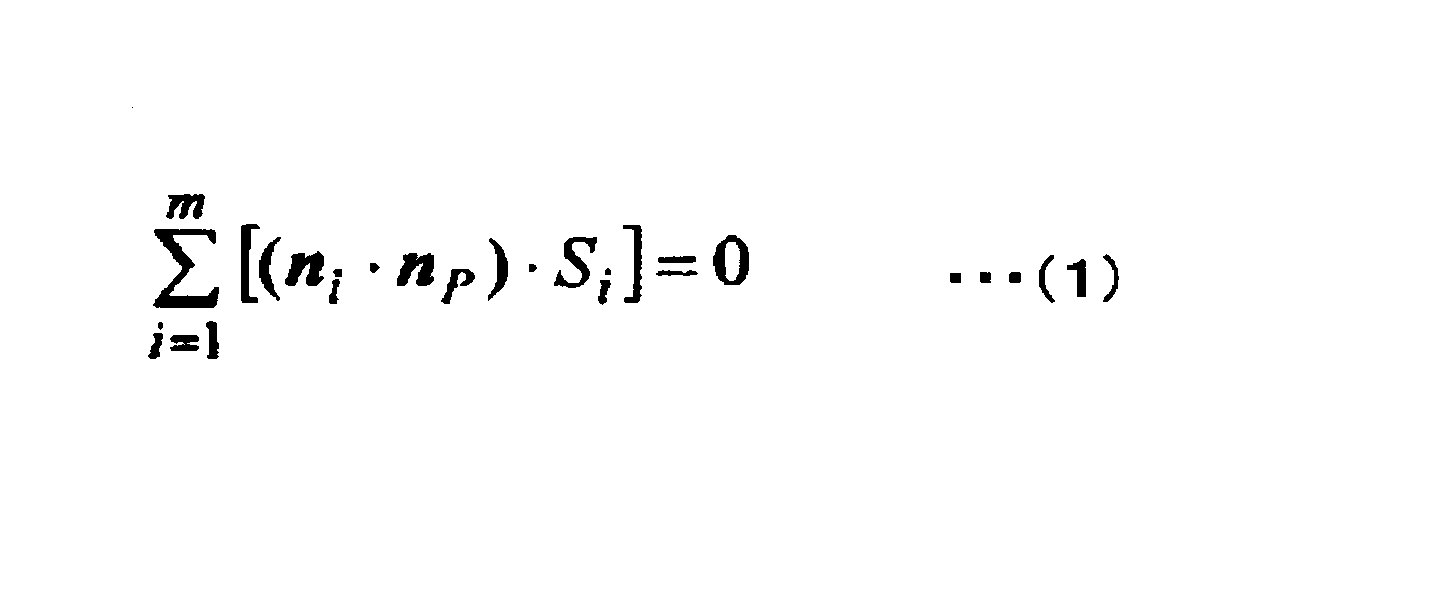
(付記5)
前記集合領域での計算用データモデルの生成において、
全集合領域の体積の総和が解析領域の体積と一致するという条件と、
隣り合う前記集合領域同士の境界面の面積が一致するという条件及び法線ベクトルが当該境界面を挟む一方の集合領域から見た場合と他方の集合領域から見た場合とで絶対値が一致するという条件と、
前記集合領域を通る無限に広い投影面Pの任意の向きの単位法線ベクトルが[N]P、境界面の面積がQi、境界面の単位法線ベクトルが[N]i、集合領域の面の総数がM、前記[]で囲まれた文字がベクトルを示す太字であるときに下式(2)が成り立つという条件と、
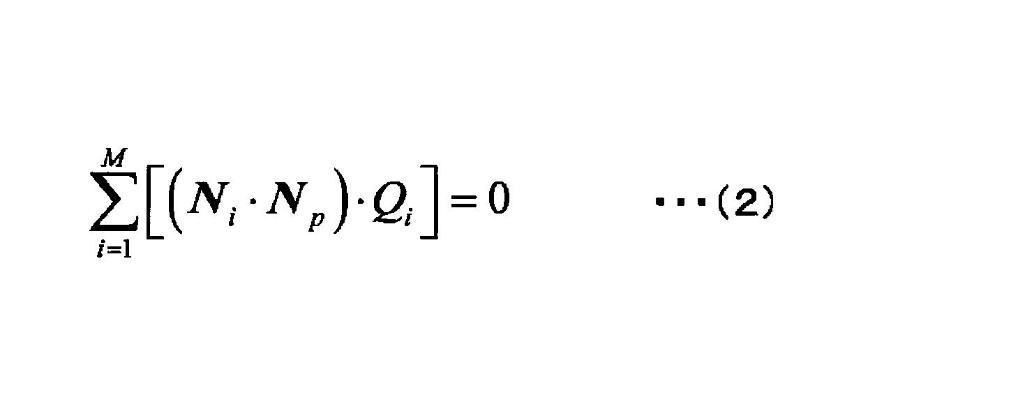
(付記6)
前記分割領域特性量は、隣り合う前記分割領域同士の境界面の特性を示す境界面特性量と、隣り合う前記分割領域同士の結合情報と、隣り合う前記分割領域同士の距離とからなり、
前記集合領域特性量は、隣り合う前記集合領域同士の境界面の特性を示す境界面特性量と、隣り合う前記集合領域同士の結合情報と、隣り合う前記集合領域同士の距離とからなる、
付記1から5のいずれか一項に記載の方法。
(付記7)
前記隣り合う前記分割領域同士の境界面の特性を示す境界面特性量は、前記隣り合う前記分割領域同士の境界面の面積と前記境界面との法線ベクトルであり、
前記隣り合う前記集合領域同士の境界面の特性を示す前記境界面特性量は、前記隣り合う前記集合領域同士の境界面の面積と前記境界面の法線ベクトルとである、
付記6に記載の方法。
(付記8)
前記分割領域での計算用データモデルの生成において、前記分割領域の体積と隣り合う前記分割領域同士の特性を示す前記分割領域特性量とを前記分割領域の頂点の座標(Vertex)及び該頂点の連結情報(Connectivity)から得る、付記1から7のいずれか一項に記載の方法。
(付記9)
コンピュータに、外部装置から解析領域の3次元形状データを取得させて前記解析領域を複数の分割領域に分割させ、
前記分割領域の頂点の座標(Vertex)及び該頂点の連結情報(Connectivity)を必要としない量のみを使用すると共に重み付き残差積分法に基づいて導出された離散化された分割領域での支配方程式に基づき、各前記分割領域の体積と隣り合う前記分割領域同士の特性を示す分割領域特性量とを前記分割領域の頂点の座標(Vertex)及び該頂点の連結情報(Connectivity)を必要としない量として有する前記分割領域での計算用データモデルを生成させ、
前記分割領域を複数集合させることによって、要求される数の集合領域を生成させ、
前記集合領域の頂点の座標(Vertex)及び該頂点の連結情報(Connectivity)を必要としない量のみを使用すると共に重み付き残差積分法に基づいて導出された離散化された集合領域での支配方程式に基づき、各前記集合領域の体積と隣り合う前記集合領域同士の特性を示す集合領域特性量とを前記集合領域の頂点の座標(Vertex)及び該頂点の連結情報(Connectivity)を必要としない量として有する前記集合領域での計算用データモデルを生成させ、
前記解析領域での物性値と、前記集合領域での計算用データモデルとに基づいて、前記集合領域での解析結果である物理量を計算させる、ことを特徴とする物理量計算プログラム。
(付記10)
物理現象での物理量を数値的に解析する物理量計算装置であって、
データを表示する出力装置と、
外部装置との間においてデータの受け渡しを行う通信装置と、
前記通信装置を介して前記外部装置から解析領域の3次元形状データを取得し、前記解析領域を複数の分割領域に分割し、前記分割領域を複数集合させることによって、要求される数の集合領域を生成する演算部と、
前記分割領域の頂点の座標(Vertex)及び該頂点の連結情報(Connectivity)を必要としない量のみを使用すると共に重み付き残差積分法によって導出された離散化された分割領域での支配方程式と、前記集合領域の頂点の座標(Vertex)及び該頂点の連結情報(Connectivity)を必要としない量のみを使用すると共に重み付き残差積分法によって導出された離散化された集合領域での支配方程式とを記憶する記憶部とを備え、
前記演算部は、前記記憶部に記憶された前記分割領域での支配方程式に基づき、各前記分割領域の体積と隣り合う前記分割領域同士の特性を示す分割領域特性量とを前記分割領域の頂点の座標(Vertex)及び該頂点の連結情報(Connectivity)を必要としない量として有する前記分割領域での計算用データモデルを生成し、前記記憶部に記憶された前記集合領域での支配方程式に基づき、各前記集合領域の体積と隣り合う前記集合領域同士の特性を示す集合領域特性量とを前記集合領域の頂点の座標(Vertex)及び該頂点の連結情報(Connectivity)を必要としない量として有する前記集合領域での計算用データモデルを生成し、前記解析領域での物性値と、前記集合領域での計算用データモデルとに基づいて、前記集合領域での解析結果である物理量を計算し、
前記解析結果である物理量の可視化データを生成して前記出力装置に表示することを特徴とする物理量計算装置。
A……数値解析装置(物理量計算装置)
P……数値解析プログラム
P1……プリ処理プログラム
P2……ソルバ処理プログラム(物理量計算プログラム)
P3……ポスト処理プログラム
M1……第一計算用データモデル
M2……第二計算用データモデル
1……CPU
2……記憶装置
2a……プログラム記憶部
2b……データ記憶部
3……DVDドライブ
4……入力装置
4a……キーボード
4b……マウス
5……出力装置
5a……ディスプレイ
5b……プリンタ
P……数値解析プログラム
P1……プリ処理プログラム
P2……ソルバ処理プログラム(物理量計算プログラム)
P3……ポスト処理プログラム
M1……第一計算用データモデル
M2……第二計算用データモデル
1……CPU
2……記憶装置
2a……プログラム記憶部
2b……データ記憶部
3……DVDドライブ
4……入力装置
4a……キーボード
4b……マウス
5……出力装置
5a……ディスプレイ
5b……プリンタ
Claims (8)
- コンピュータによって物理現象での物理量を数値的に解析するシミュレーション方法であって、
コンピュータが、解析領域を複数の分割領域に分割し、
前記分割領域の頂点の座標(Vertex)及び該頂点の連結情報(Connectivity)を必要としない量のみを使用すると共に重み付き残差積分法に基づいて導出された離散化された分割領域での支配方程式に基づき、各前記分割領域の体積と隣り合う前記分割領域同士の特性を示す分割領域特性量とを前記分割領域の頂点の座標(Vertex)及び該頂点の連結情報(Connectivity)を必要としない量として有する前記分割領域での計算用データモデルを生成し、
前記分割領域を複数集合させることによって、要求される数の集合領域を生成し、
前記集合領域の頂点の座標(Vertex)及び該頂点の連結情報(Connectivity)を必要としない量のみを使用すると共に重み付き残差積分法に基づいて導出された離散化された集合領域での支配方程式に基づき、各前記集合領域の体積と隣り合う前記集合領域同士の特性を示す集合領域特性量とを前記集合領域の頂点の座標(Vertex)及び該頂点の連結情報(Connectivity)を必要としない量として有する前記集合領域での計算用データモデルを生成し、
前記解析領域での物性値と、前記集合領域での計算用データモデルとに基づいて、前記集合領域での解析結果である物理量を計算する、ことを特徴とするシミュレーション方法。 - 前記分割領域での計算用データモデルの生成において、
全分割領域の体積の総和が解析領域の体積と一致するという条件と、
前記分割領域同士の境界面の面積が一致するという条件及び法線ベクトルが当該境界面を挟む一方の分割領域から見た場合と他方の分割領域から見た場合とで絶対値が一致するという条件と、
前記分割領域を通る無限に広い投影面Pの任意の向きの単位法線ベクトルが[n]p、境界面の面積がSi、境界面の単位法線ベクトルが[n]i、分割領域の面の総数がm、前記[]で囲まれた文字がベクトルを示す太字であるときに下式(1)が成り立つという条件と、
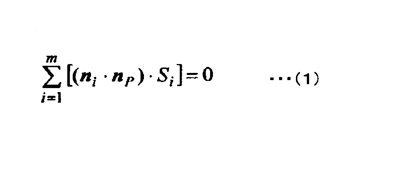
- 前記集合領域での計算用データモデルの生成において、
全集合領域の体積の総和が解析領域の体積と一致するという条件と、
隣り合う前記集合領域同士の境界面の面積が一致するという条件及び法線ベクトルが当該境界面を挟む一方の集合領域から見た場合と他方の集合領域から見た場合とで絶対値が一致するという条件と、
前記集合領域を通る無限に広い投影面Pの任意の向きの単位法線ベクトルが[N]P、境界面の面積がQi、境界面の単位法線ベクトルが[N]i、集合領域の面の総数がM、前記[]で囲まれた文字がベクトルを示す太字であるときに下式(2)が成り立つという条件と、

- 前記分割領域特性量は、隣り合う前記分割領域同士の境界面の特性を示す境界面特性量と、隣り合う前記分割領域同士の結合情報と、隣り合う前記分割領域同士の距離とからなり、
前記集合領域特性量は、隣り合う前記集合領域同士の境界面の特性を示す境界面特性量と、隣り合う前記集合領域同士の結合情報と、隣り合う前記集合領域同士の距離とからなる、
請求項1から3のいずれか一項に記載の方法。 - 前記隣り合う前記分割領域同士の境界面の特性を示す境界面特性量は、前記隣り合う前記分割領域同士の境界面の面積と前記境界面との法線ベクトルであり、
前記隣り合う前記集合領域同士の境界面の特性を示す前記境界面特性量は、前記隣り合う前記集合領域同士の境界面の面積と前記境界面の法線ベクトルとである、
請求項4に記載の方法。 - 前記分割領域での計算用データモデルの生成において、前記分割領域の体積と隣り合う前記分割領域同士の特性を示す前記分割領域特性量とを前記分割領域の頂点の座標(Vertex)及び該頂点の連結情報(Connectivity)から得る、請求項1から5のいずれか一項に記載の方法。
- コンピュータに、解析領域を複数の分割領域に分割させ、
前記分割領域の頂点の座標(Vertex)及び該頂点の連結情報(Connectivity)を必要としない量のみを使用すると共に重み付き残差積分法に基づいて導出された離散化された分割領域での支配方程式に基づき、各前記分割領域の体積と隣り合う前記分割領域同士の特性を示す分割領域特性量とを前記分割領域の頂点の座標(Vertex)及び該頂点の連結情報(Connectivity)を必要としない量として有する前記分割領域での計算用データモデルを生成させ、
前記分割領域を複数集合させることによって、要求される数の集合領域を生成させ、
前記集合領域の頂点の座標(Vertex)及び該頂点の連結情報(Connectivity)を必要としない量のみを使用すると共に重み付き残差積分法に基づいて導出された離散化された集合領域での支配方程式に基づき、各前記集合領域の体積と隣り合う前記集合領域同士の特性を示す集合領域特性量とを前記集合領域の頂点の座標(Vertex)及び該頂点の連結情報(Connectivity)を必要としない量として有する前記集合領域での計算用データモデルを生成させ、
前記解析領域での物性値と、前記集合領域での計算用データモデルとに基づいて、前記集合領域での解析結果である物理量を計算させる、ことを特徴とする物理量計算プログラム。 - 物理現象での物理量を数値的に解析する物理量計算装置であって、
解析領域を複数の分割領域に分割し、前記分割領域を複数集合させることによって、要求される数の集合領域を生成する演算部と、
前記分割領域の頂点の座標(Vertex)及び該頂点の連結情報(Connectivity)を必要としない量のみを使用すると共に重み付き残差積分法によって導出された離散化された分割領域での支配方程式と、前記集合領域の頂点の座標(Vertex)及び該頂点の連結情報(Connectivity)を必要としない量のみを使用すると共に重み付き残差積分法によって導出された離散化された集合領域での支配方程式とを記憶する記憶部とを備え、
前記演算部は、前記記憶部に記憶された前記分割領域での支配方程式に基づき、各前記分割領域の体積と隣り合う前記分割領域同士の特性を示す分割領域特性量とを前記分割領域の頂点の座標(Vertex)及び該頂点の連結情報(Connectivity)を必要としない量として有する前記分割領域での計算用データモデルを生成し、前記記憶部に記憶された前記集合領域での支配方程式に基づき、各前記集合領域の体積と隣り合う前記集合領域同士の特性を示す集合領域特性量とを前記集合領域の頂点の座標(Vertex)及び該頂点の連結情報(Connectivity)を必要としない量として有する前記集合領域での計算用データモデルを生成し、前記解析領域での物性値と、前記集合領域での計算用データモデルとに基づいて、前記集合領域での解析結果である物理量を計算する、ことを特徴とする物理量計算装置。
Priority Applications (3)
| Application Number | Priority Date | Filing Date | Title |
|---|---|---|---|
| CN201880063617.4A CN111247601A (zh) | 2018-09-12 | 2018-11-28 | 模拟方法、物理量计算程序及物理量计算装置 |
| JP2019506743A JP6504333B1 (ja) | 2018-09-12 | 2018-11-28 | シミュレーション方法、物理量計算プログラム及び物理量計算装置 |
| US16/285,261 US20200082035A1 (en) | 2018-09-12 | 2019-02-26 | Simulation method, physical quantity calculation program, and physical quantity calculation apparatus |
Applications Claiming Priority (2)
| Application Number | Priority Date | Filing Date | Title |
|---|---|---|---|
| JP2018-170766 | 2018-09-12 | ||
| JP2018170766 | 2018-09-12 |
Related Child Applications (1)
| Application Number | Title | Priority Date | Filing Date |
|---|---|---|---|
| US16/285,261 Continuation US20200082035A1 (en) | 2018-09-12 | 2019-02-26 | Simulation method, physical quantity calculation program, and physical quantity calculation apparatus |
Publications (1)
| Publication Number | Publication Date |
|---|---|
| WO2020054087A1 true WO2020054087A1 (ja) | 2020-03-19 |
Family
ID=66396952
Family Applications (1)
| Application Number | Title | Priority Date | Filing Date |
|---|---|---|---|
| PCT/JP2018/043836 Ceased WO2020054087A1 (ja) | 2018-09-12 | 2018-11-28 | シミュレーション方法、物理量計算プログラム及び物理量計算装置 |
Country Status (2)
| Country | Link |
|---|---|
| CN (1) | CN111247601A (ja) |
| WO (1) | WO2020054087A1 (ja) |
Families Citing this family (1)
| Publication number | Priority date | Publication date | Assignee | Title |
|---|---|---|---|---|
| CN114266179B (zh) * | 2021-12-23 | 2023-08-04 | 成都理工大学 | 基于有限单元的矿床钻探信息处理及分析方法和装置 |
Citations (2)
| Publication number | Priority date | Publication date | Assignee | Title |
|---|---|---|---|---|
| WO2010150758A1 (ja) * | 2009-06-25 | 2010-12-29 | 旭硝子株式会社 | 物理量計算方法、数値解析方法、物理量計算プログラム、数値解析プログラム、物理量計算装置及び数値解析装置 |
| WO2012026383A1 (ja) * | 2010-08-24 | 2012-03-01 | 旭硝子株式会社 | 計算用データ生成装置、計算用データ生成方法及び計算用データ生成プログラム |
Family Cites Families (8)
| Publication number | Priority date | Publication date | Assignee | Title |
|---|---|---|---|---|
| US5946211A (en) * | 1997-02-28 | 1999-08-31 | The Whitaker Corporation | Method for manufacturing a circuit on a circuit substrate |
| JP2004046379A (ja) * | 2002-07-09 | 2004-02-12 | Tadahiko Kawai | 無節点有限要素法 |
| US8295262B2 (en) * | 2006-08-15 | 2012-10-23 | Texas Instruments Incorporated | Uplink reference signal for time and frequency scheduling of transmissions |
| CN101784114B (zh) * | 2009-01-16 | 2012-07-25 | 电信科学技术研究院 | 多小区协同的数据传输方法、系统及装置 |
| JP2012118666A (ja) * | 2010-11-30 | 2012-06-21 | Iwane Laboratories Ltd | 三次元地図自動生成装置 |
| JP5487264B2 (ja) * | 2012-09-07 | 2014-05-07 | 三菱プレシジョン株式会社 | 生体データモデル作成方法及びその装置 |
| US20140222384A1 (en) * | 2013-02-04 | 2014-08-07 | Comsol Ab | Apparatus and method for defining coupled systems on spatial dimensions and extra dimensions |
| US10280722B2 (en) * | 2015-06-02 | 2019-05-07 | Baker Hughes, A Ge Company, Llc | System and method for real-time monitoring and estimation of intelligent well system production performance |
-
2018
- 2018-11-28 WO PCT/JP2018/043836 patent/WO2020054087A1/ja not_active Ceased
- 2018-11-28 CN CN201880063617.4A patent/CN111247601A/zh active Pending
Patent Citations (2)
| Publication number | Priority date | Publication date | Assignee | Title |
|---|---|---|---|---|
| WO2010150758A1 (ja) * | 2009-06-25 | 2010-12-29 | 旭硝子株式会社 | 物理量計算方法、数値解析方法、物理量計算プログラム、数値解析プログラム、物理量計算装置及び数値解析装置 |
| WO2012026383A1 (ja) * | 2010-08-24 | 2012-03-01 | 旭硝子株式会社 | 計算用データ生成装置、計算用データ生成方法及び計算用データ生成プログラム |
Non-Patent Citations (1)
| Title |
|---|
| OHATA, AKIRA: "Complex Physical Region Modeling for Model-Based Development. First Edition", 30 November 2012, TECHSHARE, ISBN: 978-4-906864-02-7, pages: 55 - 65, XP009514337 * |
Also Published As
| Publication number | Publication date |
|---|---|
| CN111247601A (zh) | 2020-06-05 |
Similar Documents
| Publication | Publication Date | Title |
|---|---|---|
| JP6516081B1 (ja) | シミュレーション方法、mbdプログラムによるシミュレーション方法、数値解析装置、mbd用数値解析システム、数値解析プログラムおよびmbdプログラム | |
| CN102804187B (zh) | 物理量计算方法、数值解析方法、物理量计算装置及数值解析装置 | |
| Gano et al. | Hybrid variable fidelity optimization by using a kriging-based scaling function | |
| JP5045853B2 (ja) | 計算用データ生成装置、計算用データ生成方法及び計算用データ生成プログラム | |
| JP6504333B1 (ja) | シミュレーション方法、物理量計算プログラム及び物理量計算装置 | |
| CN110852003B (zh) | 计算机辅助设计定义的几何形状中的对象间的间隙的检测 | |
| Gagnon et al. | Two-level free-form deformation for high-fidelity aerodynamic shape optimization | |
| EP4510034A1 (en) | Fluid flow simulation | |
| WO2020054086A1 (ja) | シミュレーション方法、mbdプログラムによるシミュレーション方法、数値解析装置、mbd用数値解析システム、数値解析プログラムおよびmbdプログラム | |
| Krakos et al. | Gpu-based and adaptive solution technology for the 5th aiaa high lift prediction workshop | |
| WO2017112581A1 (en) | Composite design direction | |
| CN111247601A (zh) | 模拟方法、物理量计算程序及物理量计算装置 | |
| Fenwick et al. | Development and validation of sliding and non-matching grid technology for control surface representation | |
| Liu et al. | Edge based viscous method for node-centered formulations | |
| CN110909511B (zh) | 一种无曲面体积分的无粘低速绕流数值模拟方法 | |
| Liatsikouras et al. | A coupled CAD‐free parameterization‐morphing method for adjoint‐based shape optimization | |
| Shen et al. | Towards a framework for parametric models and geometric sensitivity computations with SU2 and pyCAPS | |
| Lakshminarayan et al. | Fully Automated Surface Mesh Adaptation in Strand Grid Framework | |
| Tarsia Morisco et al. | Extension of the Vertex-Centered Mixed-Element-Volume MUSCL scheme to mixed-element meshes | |
| Tarsia Morisco et al. | Validation of the Spalart-Allmaras QCR2000-R Turbulence Model using anisotropic mesh adaptation on HFCFDV Workshop test cases | |
| McComas et al. | Automated Method for Rapid Estimation of Aeroelastic Wing Shapes–TLG StarBEAM | |
| Barutcu et al. | A Parametric Modeling Approach for Prediction of Load Distribution due to Fluid Structure Interaction on Aircraft Structures | |
| Kühner et al. | From a product model to visualization: Simulation of indoor flows with lattice‐Boltzmann methods | |
| Cella et al. | Integration within Fluid Dynamic Solvers of an Advanced Geometric Parameterization Based on Mesh Morphing. Fluids 2022, 7, 310 | |
| Poole et al. | Metric-based mathematical derivation of aerofoil design variables |
Legal Events
| Date | Code | Title | Description |
|---|---|---|---|
| ENP | Entry into the national phase |
Ref document number: 2019506743 Country of ref document: JP Kind code of ref document: A |
|
| ENP | Entry into the national phase |
Ref document number: 2018847205 Country of ref document: EP Effective date: 20190227 |
|
| NENP | Non-entry into the national phase |
Ref country code: DE |