WO2019026523A1 - クラスタリングの評価値算出方法及びクラスタ数決定方法 - Google Patents
クラスタリングの評価値算出方法及びクラスタ数決定方法 Download PDFInfo
- Publication number
- WO2019026523A1 WO2019026523A1 PCT/JP2018/025498 JP2018025498W WO2019026523A1 WO 2019026523 A1 WO2019026523 A1 WO 2019026523A1 JP 2018025498 W JP2018025498 W JP 2018025498W WO 2019026523 A1 WO2019026523 A1 WO 2019026523A1
- Authority
- WO
- WIPO (PCT)
- Prior art keywords
- cluster
- clusters
- evaluation value
- value
- data
- Prior art date
- Legal status (The legal status is an assumption and is not a legal conclusion. Google has not performed a legal analysis and makes no representation as to the accuracy of the status listed.)
- Ceased
Links
Images




Classifications
-
- G—PHYSICS
- G06—COMPUTING OR CALCULATING; COUNTING
- G06F—ELECTRIC DIGITAL DATA PROCESSING
- G06F16/00—Information retrieval; Database structures therefor; File system structures therefor
- G06F16/90—Details of database functions independent of the retrieved data types
- G06F16/906—Clustering; Classification
-
- G—PHYSICS
- G06—COMPUTING OR CALCULATING; COUNTING
- G06F—ELECTRIC DIGITAL DATA PROCESSING
- G06F18/00—Pattern recognition
- G06F18/20—Analysing
- G06F18/21—Design or setup of recognition systems or techniques; Extraction of features in feature space; Blind source separation
- G06F18/217—Validation; Performance evaluation; Active pattern learning techniques
-
- G—PHYSICS
- G06—COMPUTING OR CALCULATING; COUNTING
- G06F—ELECTRIC DIGITAL DATA PROCESSING
- G06F18/00—Pattern recognition
- G06F18/20—Analysing
- G06F18/23—Clustering techniques
- G06F18/232—Non-hierarchical techniques
-
- G—PHYSICS
- G06—COMPUTING OR CALCULATING; COUNTING
- G06F—ELECTRIC DIGITAL DATA PROCESSING
- G06F18/00—Pattern recognition
- G06F18/20—Analysing
- G06F18/24—Classification techniques
- G06F18/241—Classification techniques relating to the classification model, e.g. parametric or non-parametric approaches
- G06F18/2413—Classification techniques relating to the classification model, e.g. parametric or non-parametric approaches based on distances to training or reference patterns
- G06F18/24133—Distances to prototypes
- G06F18/24137—Distances to cluster centroïds
-
- G—PHYSICS
- G06—COMPUTING OR CALCULATING; COUNTING
- G06N—COMPUTING ARRANGEMENTS BASED ON SPECIFIC COMPUTATIONAL MODELS
- G06N20/00—Machine learning
Definitions
- the present invention relates to a method of calculating an evaluation value of clustering and a method of determining the number of clusters.
- Clustering that classifies a plurality of data sets to be classified into a plurality of clusters (data groups) is known, and in recent years, it is frequently used in image analysis, data mining, big data analysis, etc. .
- clustering similar data are classified into the same cluster, and classification is performed so that the data is not as similar as possible among the clusters, and data tendency or feature extraction is performed from the classification result.
- a clustering method for classifying a plurality of data into clusters and the k-means method is known as one of the representative clustering methods.
- the number k of clusters is set in advance, for example, arbitrary k data are selected from all the N data, and they are used as initial values of the centers of gravity of k clusters (Procedure 1) .
- each piece of data is classified into a cluster of centroids with the shortest distance to the data (Procedure 2).
- For each cluster set the average of the data in the cluster to the center of gravity of the new cluster (Procedure 3). Then, step 2 and step 3 are repeated until the center of gravity of each cluster does not change.
- the above-described clustering method classifies data into clusters of a preset number of clusters, and the number of clusters needs to be preset.
- the evaluation value for each of the results obtained by changing the number of clusters is determined, and the evaluation value is an extreme value or an optimum number of clusters with maximum to minimum values. It is a number.
- VRC (hereinafter referred to as evaluation value VRC) is known as one of representative ones (for example, Non-Patent Document 1).
- the evaluation value VRC is a ratio of the degree of external separation normalized by the number of clusters to the degree of internal coupling normalized by the total number of data.
- the value before normalization of the external separation degree in the evaluation value VRC is the sum of the respective values of the clusters weighted by the number of data in the cluster to the distance between the centroid of all the data and the centroid of the cluster. Further, the value before normalization of the degree of internal coupling in the evaluation value VRC is the sum of the distance between the center of gravity of the cluster and each data in the cluster for each cluster.
- the evaluation value VRC when used, if there is a large data grouping or a high data distribution density with respect to other data in all the data, the large range There is a tendency for the number of clusters to be large by excessively classifying data aggregation and data aggregation having high distribution density. That is, the evaluation value VRC tends to be larger in the case where classification of data in such a large range or data having a high distribution density is classified into a plurality of clusters rather than classification into a single cluster.
- the present invention has been made in view of the above circumstances, and an evaluation value calculation method of clustering capable of obtaining an evaluation value for evaluating a clustering state capable of suppressing excessive classification and a cluster using the evaluation value
- the purpose is to provide a number determination method.
- the present invention provides an evaluation value calculation method of clustering in which an evaluation value of a clustering state is calculated by the number of clusters when a plurality of data are clustered, an acquisition step of acquiring information on clustered data, and the acquired Calculating the evaluation value based on the information, wherein the calculating step sets a first index value for each of the clusters indicating the degree of dispersion of data in the cluster to the number of data of the cluster.
- the internal connectivity which is the sum of each cluster of values normalized by a first value based on the first value, and the total number of second index values for each of the clusters that is an index of the distance between the clusters And the external separation degree normalized by the second value based on That is from a predetermined arithmetic expression and calculates the evaluation value.
- evaluation values for the clustering results with different numbers of clusters are calculated using the above-mentioned evaluation value calculation method, and the extremum among the evaluation values, or the maximum value or the minimum value.
- the number of clusters corresponding to the evaluation value of the value is determined as the optimum value.
- the sum of values normalized by the first value based on the number of cluster data and the first index value for each cluster indicating the degree of internal coupling as the degree of dispersion of each data in the cluster. Since the evaluation value is calculated assuming that the external separation degree is the sum of the second index value for each cluster that is an index of the distance between clusters, with the second value based on the number of clusters. It is possible to obtain an evaluation value that can suppress excessive classification.
- FIG. 10 It is a block diagram which shows the structure of the arithmetic unit which implemented this invention. It is a flowchart which shows the process sequence which acquires the clustering result in which an evaluation value becomes local maximum. It is a flowchart which shows the process sequence which acquires the clustering result in which an evaluation value becomes the maximum value. It is explanatory drawing explaining each value in the case of calculating
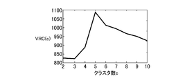
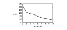
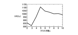
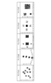
- 10 is an explanatory view showing a sample 3; It is a graph which shows change of evaluation value E1 (c) to the number of clusters of sample 1. It is a graph which shows change of evaluation value E2 (c) to the number of clusters of sample 1. It is a graph which shows change of evaluation value VRC (c) to the number of clusters of sample 1. It is a graph which shows change of evaluation value E1 (c) to the number of clusters of sample 2. It is a graph which shows change of evaluation value E2 (c) to the number of clusters of sample 2. It is a graph which shows change of evaluation value VRC (c) to the number of clusters of sample 2. It is a graph which shows change of evaluation value E1 (c) to the number of clusters of sample 3. It is a graph which shows change of evaluation value E2 (c) to the number of clusters of sample 3. It is a graph which shows change of evaluation value VRC (c) to the number of clusters of sample 3. It is explanatory drawing which shows samples AE.
- the arithmetic unit 10 performs clustering on a plurality of data, calculates an evaluation value for evaluating a clustering state, and obtains a clustering result with an optimal number of clustering based on the evaluation value. Configured In order to obtain an optimal clustering number, the arithmetic unit 10 performs clustering on a plurality of data a plurality of times by changing the number of clusters.
- the arithmetic device 10 is configured by, for example, a computer, and functions as an evaluation value arithmetic unit 11, a clustering unit 12, a control unit 13 that controls these overall, and a data storage unit 14.
- the data storage unit 14 is configured by a hard disk or a memory of a computer, and a plurality of data to be subjected to clustering are written in advance. These data are q (q is an integer of 1 or more) dimensional vectors, and for example, contents such as color, density, and color distribution of an image are q dimensional vectors.
- q is an integer of 1 or more
- contents such as color, density, and color distribution of an image are q dimensional vectors.
- the clustering unit 12 reads out data targeted for clustering from the data storage unit 14, performs clustering, and stores the result in the data storage unit 14.
- the clustering by the clustering unit 12 is performed using the k-means method described above in this example.
- the calculation method of the evaluation value by the evaluation value calculation unit 11 is not limited to the k-means method, and can be applied to hard clustering in which each data is classified to belong to one cluster. As such hard clustering, there are "k-means ++" method, spectral clustering, single connection method, Ward method and the like.
- the evaluation value calculation unit 11 calculates an evaluation value E1 (c) each time the clustering unit 12 performs clustering for one cluster number c (c is an integer of 2 or more).
- the evaluation value calculation unit 11 acquires a clustering result as information on data clustered from the data storage unit 14.
- the evaluation value calculator 11 calculates an evaluation value E1 (c) for evaluating a clustering state of the clustering result based on the acquired clustering result.
- the evaluation value calculator 11 outputs the evaluation value E1 (c) to the controller 13. The details of the calculation of the evaluation value E1 (c) will be described later.
- Information on the clustered data acquired by the evaluation value calculation unit 11 is, for example, generated during the calculation of clustering.
- the cluster centroid, intracluster distance, etc. As they are sought, they can be included and can be used to calculate the evaluation value E1 (c).
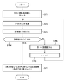
- the control unit 13 determines the optimal number of clusters c by comparing the evaluation values E1 (c) calculated by the evaluation value calculation unit 11. In this example, the control unit 13 determines that the number c of clusters corresponding to the evaluation value E1 (c) taking the extreme value (maximum value in this example) is the optimum one based on the procedure of the hill climbing method shown in FIG. Do. That is, each time the evaluation value E1 (c) is calculated, the calculated evaluation value E1 (c) is compared with the previously calculated evaluation value E1 (c), and the latter is smaller than the former. In addition, assuming that the evaluation value E1 (c) calculated at the previous time is the maximum value, the number of clusters c corresponding to the evaluation value E1 (c) is determined to be the optimum one.
- the control unit 13 initializes the number of clusters c at step ST1 and initializes the variable E0 indicating the previous evaluation value to “0”.
- the number of clusters c is set to “2” in the initialization of this example.
- the control unit 13 causes the clustering unit 12 to perform clustering by the k-means method under the set number of clusters, and at step ST3 thereafter, an evaluation value E1 for the number c of clusters based on the result of clustering. (C) is calculated by the evaluation value calculator 11.
- the number of clusters c is the number of clusters k in the k-means method described above.
- step ST4 the control unit 13 compares the evaluation value E1 (c) calculated this time with the variable E0. In this comparison, if the evaluation value E1 (c) is greater than or equal to the variable E0, the clustering unit 12 is made to perform clustering again in step ST2 after steps ST5 and ST6. In step ST5, the variable E0 is set to the evaluation value E1 (c) calculated this time, and in step ST6, the number c of clusters is incremented by "1". As a result, the cluster number c is increased by "1" and the next clustering is performed (step ST2), and the evaluation value E1 (c) newly obtained in step ST3 is compared with the previous one (step ST4) .
- the control unit 13 determines that the evaluation value E1 (c) has turned to a decrease, and corresponds to the number of clusters (c-1) in step ST7. Get the result of clustering. That is, it is determined that the number of clusters (c-1) with c being the number of clusters when clustering is last performed is an optimal value as the number of clusters.
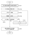
- the maximum number of clusters within the set number of clusters c may be determined as the optimum value.
- the range of the number c of clusters to be evaluated is set by initially setting the initial value and the set maximum value of the number c of clusters in step ST11.
- the control unit 13 sets the number of clusters c to an initial value.
- clustering is performed by the clustering unit 12 under the number c of clusters set in step ST12, and in step ST14 thereafter, the evaluation value E1 (c) for the number c of clusters based on the clustering result is evaluated value calculation Let part 11 calculate.
- step ST15 it is checked whether the number of clusters c is greater than or equal to the set maximum value.
- step ST16 If the number c of clusters does not reach the set maximum value, the number c of clusters is incremented by “1” in step ST16, and then clustering according to step ST13 is performed again. Thus, clustering is repeatedly performed while incrementing the number of clusters c by “1” until the number of clusters c reaches the set maximum value, and the evaluation value E1 (c) is calculated for each clustering. Then, after completion of clustering for the set maximum number of clusters c, the evaluation values E1 (c) for each cluster number c are compared, and the number of clusters c corresponding to the maximum evaluation value E1 (c) among them is compared. It is determined that the value is an optimal value, and the control unit 13 acquires a clustering result corresponding to the number of clusters c (step ST17).
- the evaluation value E1 (c) calculated by the evaluation value calculator 11 is expressed as equation (1).
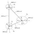
- FIG. 4 schematically shows an example of data x, i-th cluster c i , center of gravity v i of cluster c i , inter-cluster distance dist (v i , v j ), and intra-cluster distance dist (x, v i ) Shown in.
- n Number of data targeted for clustering (total number of data)
- x data
- data c number of clusters c i : i-th cluster
- n i number of data in cluster c i
- v i center of gravity of cluster c i (cluster center of gravity)
- the denominator on the right side of Equation (1) is an internal degree of coupling that indicates the degree of data distribution (similarity between data) in a cluster for all clusters.
- the first representative point is the cluster centroid
- the degree of internal coupling is obtained as the sum of the normalized values for each cluster by dividing the first index value for each cluster by the number of data in the cluster.
- the first index value of each cluster indicates the degree of dispersion of data in the corresponding cluster, and in this example, it is the sum of intra-cluster distance index values for each data in the corresponding cluster.
- the numerator on the right side of Equation (1) is an external degree of separation that indicates the degree of separation of clusters for all clusters.
- the degree of external separation is a value obtained by dividing the sum of the second index values for each cluster for each cluster by the number of clusters and normalizing the sum.
- the second index value is a degree of separation between one cluster and each of the other clusters, that is, a value indicative of the distance between clusters for the one cluster, and in this example, the cluster for each cluster This is the minimum value of the inter-distance index value.
- both the intra-cluster distance and the inter-cluster distance are Euclidean distances. Assuming that data which is two q-dimensional vectors are a (a 1 , a 2 ,... A q ) and b (b 1 , b 2 ,... B q ), the Euclidean distance between a and b is , Is expressed as equation (A).
- the external separation degree is a value obtained by normalizing the sum of the second index value serving as an index of the degree of separation of clusters for each cluster by the number of clusters
- the degree of internal coupling is a sum of values obtained by normalizing the first index value indicating the degree of dispersion of each data in each cluster to the number of data in each cluster. For this reason, even if there is a large area of data group or another high data distribution density with respect to other data groups in all the data, etc., within each cluster. The degree of dispersion of data is properly reflected in the degree of internal coupling. That is, when the classification is excessive, the evaluation value E1 (c) does not become larger and the excessive classification is suppressed.
- the number c of clusters may be determined so that the evaluation value E1 (c) takes the maximum value or the maximum value.
- the number c of clusters may be determined so that the evaluation value E1 (c) takes a minimum value or a minimum value.
- the second index value which is an index of the distance between clusters, is obtained using the inter-cluster distance index value, but as in the evaluation value E2 (c) shown in equation (2) Alternatively, a value determined using a reference point inter-cluster distance index value indicating the extent of the distance from a reference point set in advance to a cluster can be used as a second index value.
- the evaluation value E2 (c) will be described in detail later, the number of operations when obtaining it is smaller than that of the evaluation value E1 (c).
- each value in Formula (2) is as follows.
- the other values are the same as those of equation (1), and in this example, the reference point is the center of gravity of all n data to be subjected to clustering.
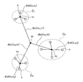
- 5 shows, the data x, i th cluster c i, cluster c i of the center of gravity v i, the reference point cluster distance dist (v i, m), schematically an example of a cluster within the distance dist (x, v i) Show.
- m a reference point D (vi, m): cluster c i of the reference point distance between clusters index value dist (vi, m): distance between the cluster centroids and the reference point of the cluster c i (distance between the reference point cluster)
- the numerator on the right side is the degree of external separation
- the denominator on the right side is the degree of internal coupling, as in the case of the equation (1) of the evaluation value E1 (c).
- the degree of external separation of the evaluation value E2 (c) is the sum of the second index values for each cluster, but the second inter-cluster distance index value is weighted by the number of data in the cluster. It is used as an index value.
- the reference point inter-cluster distance index value uses the center of gravity of all n pieces of data to be clustered (hereinafter referred to as the data center of gravity) as a reference point, and a second base point of the distance on the clustering side with respect to the reference point.
- the weighting value is not limited to the number of data in the cluster, and may be weighted based on the number of data in the cluster.
- the degree of external separation is the sum of the second index value for each cluster, which is an index of the distance between clusters.
- the evaluation value E2 (c) does not become larger, and the excessive classification is suppressed.
- the evaluation value E2 (c) increases in value according to the degree if the clustering state is good. Therefore, the number c of clusters may be determined so that the evaluation value E2 (c) takes the maximum value or the maximum value.
- the number c of clusters may be determined so that the evaluation value E2 (c) takes a minimum value or a minimum value.
- the corresponding Euclidean distance in-cluster distance as an intra-cluster distance index value, inter-cluster distance index value, reference point inter-cluster distance index value
- the corresponding Euclidean distance itself can also be used.
- the amount of calculation can be less than using the Euclidean distance itself.
- the intra-cluster distance, inter-cluster distance, and reference point inter-cluster distance in the evaluation value E1 (c) and the evaluation value E2 (c) are not limited to the Euclidean distance.
- the Manhattan distance shown in equation (B) or the Minkowski distance shown in equation (C) may be used.
- "Point symmetry distance" or the like may be used.
- the second representative points, which are the base points on the cluster side of the distances, are all at the cluster centroid, but this is not a limitation.
- the first representative point and the second representative point may be data closest to the cluster centroid within each cluster.
- the second representative point is a base point in measuring the distance (distance) between clusters or between the reference point and the cluster, the second representative point is in the adjacent cluster or in the cluster closest to or the farthest from the reference point. It is good also as data etc.
- the first representative point and the second representative point may be points or data in a cluster determined by a separately defined reference, or any points or data in a cluster.
- the reference point of the equation (2) can be set to any point or data, and in addition to the data centroid as described above, data closest to the data centroid, the second representative point of any cluster, the outside It may be a point or data determined according to a separately defined reference such as a point or data to be specified, data stored at an address of a storage device specified from the outside, data initially input, or the like.
- the first index value is normalized by the number n i of data of the cluster as the first value.
- the first value for normalization is not limited to this, and can be a value based on the number n i of data of the cluster.
- power of the data number n i of the cluster (n i 2, n i 3, n i 1/2, n i -2, etc.), the number of fixed data number n i constant multiple values, the number of data n i
- the second value is not limited to this, and a standard based on a value based on the number c of clusters Can be As a value based on the number of clusters other than the number c of clusters, similarly to the first value, for example, ⁇ ⁇ ⁇ ⁇ of the number c of clusters, a value obtained by multiplying the number c of clusters by a constant, a value obtained by subtracting or adding a fixed number to the number c of clusters.
- G (n, c) the second value.
- the evaluation value E1 (c) and the evaluation value E2 (c) are operations for obtaining the evaluation value as a ratio between the internal coupling degree and the external separation degree. It is not limited to.
- the degree of internal coupling determined as described above means that the smaller the value, the more clustered the data in each cluster is such that the similarity between the data in the cluster is higher.
- the degree of external separation determined as described above means that the larger the value is, the clustering states are separated from each other so that the similarity between clusters is lower.
- the operation for obtaining the evaluation value from the degree of internal coupling and the degree of external separation is evaluated when the degree of internal coupling changes in the direction of decreasing the degree of external coupling or in the direction of increasing the degree of external separation
- the value may be changed to either increase or decrease, and an arithmetic expression having as variables the internal coupling degree and the external separation degree capable of obtaining such a result may be used.
- the internal coupling degree and the external separation degree The evaluation value E is obtained by weighting and adding the reciprocals of one and the other to each other, and the evaluation value E is obtained by weighting and subtracting the other from one of the internal coupling degree and the external separation degree.
- the value Comp in the formula is the degree of internal coupling
- Sep is the degree of external separation
- Wa and Wb are weighting constants
- E Wb ⁇ Sep + Wa ⁇ (1 / Comp)
- first and second embodiments will be described in which the sample data is clustered and the optimal number of clusters is determined using the evaluation value E1 (c) and the evaluation value E2 (c).
- the k-means method is used as the clustering method, and the procedure shown in FIG. 3 is used as the procedure for determining the optimal number of clusters to maximize the evaluation value.
- the range of clustering number is 2-10.
- Comparative Example 1 under the same conditions, the optimal number of clusters was determined using the evaluation value VRC (c) described in Non-Patent Document 1.
- Equation (3) The equation for calculating the evaluation value VRC (c) is shown in equation (3).
- each value of Formula (3) is the same as the former of Formula (1) or Formula (2).
- the value of the denominator in equation (6) indicates the degree of internal coupling
- the value of the numerator indicates the degree of external separation.
- sample 1 data are distributed at the same density in a small area separated from each other and in a large area larger in size than this small area.
- the number of data in the small area is 100
- the number of data in the large area is 400
- the large area is four times the area of the small area.
- the evaluation value E1 (c) and the evaluation value E2 (c) becomes maximum when the cluster number c is "2", and the state of clustering at that time is shown in FIG. As shown, the data of the small area and the data of the large area are classified into one cluster each. This result is consistent with human sensory judgment on the distribution of the sample 1 data.
- the evaluation value VRC (c) when the cluster number c is “5”, the evaluation value is maximum, and the state of clustering at that time is as shown in FIG. The data is classified into one cluster, and the large area data is classified into four clusters.
- the state of clustering is any of evaluation value E1 (c), evaluation value E2 (c), and evaluation value VRC (c) It is the same.
- Sample 2 is data in which data is distributed to low density areas and high density areas of the same size separated from each other, and the density of data in high density areas is higher than that in low density areas.
- the number of data in the low density area is 50
- the number of data in the high density area is 500.
- data are distributed at different densities in small areas separated from each other and large areas larger than this small area, and the density of data in the large area is higher than that in the small area.
- the number of data is 50 in the small area and 400 in the large area, and the large area is four times the area of the small area.
- the evaluation values E1 (c) and E2 (c) become maximum when the number of clusters c is “2” as in the case of the above sample 2 and sample 3 as well as sample 1. It resulted in the data being classified into one cluster.
- the evaluation value VRC (c) is maximum for sample 2 and sample 3 when the number of clusters c is “5”, and the data of the low density region of sample 2 and the small region of sample 3 are respectively one cluster. The data in the high density area of sample 2 and the large area data of sample 3 are classified into four clusters.
- Table 1 shows the values of the evaluation values when the number of clusters c for samples 1 to 3 is “2” and “5”. In addition, the circle is put on the column of "Result” in Table 1 with respect to the evaluation value which became the maximum value.
- Table 2 shows details of the internal coupling degree and the external separation degree in the evaluation value E2 (c) and the VRC (c) when the number of clusters c is “2” and “5” for sample 1 .
- the degree of internal coupling in the evaluation value E2 (c) when the cluster number c is “5” is slightly smaller than that when the cluster number c is “2”, but the cluster number c
- the degree of internal coupling in the evaluation value VRC (c) in the case where “5” is “5” is a value which is 1/3 or less of that in the case where the number of clusters c is “2”, and is a considerably small value.
- the evaluation value E2 (c) is a sum of the intra-cluster distance index values for each cluster, that is, a value obtained by dividing the first index value for each cluster by the number n i of data in the clusters
- the sum for each cluster of is the internal coupling degree.
- the cluster number c is “2”
- the small area data and the large area data are each classified into one cluster (FIG. 6 (b))
- the cluster number c is “ In case of 5 "
- the data of the small area is classified into one cluster
- the data of the large area is classified into four clusters (FIG. 6 (c)).
- the number of clusters c is "5"
- the large area data is classified into four clusters, and the clusters for each data in those four clusters
- the internal distance index value becomes quite small.
- the internal connection degree of the evaluation value VRC (c) is a value obtained by normalizing the total sum of each cluster of the first index value by the total data number n, and the total data number n is a value that does not change. Therefore, as the number of clusters c increases and the sum of the first index values decreases considerably, the degree of internal coupling also decreases accordingly. Therefore, the degree of internal coupling in the evaluation value VRC (c) when the number of clusters c is “5” is 1/3 or less of that in the case where the number of clusters c is “2”.
- the point that the first index value is considerably reduced due to the increase of the cluster number c is exactly the same as in the case of obtaining the evaluation value E2 (c).
- the evaluation value E2 (c) as described above, the first index value for each cluster is divided by the number n i of data in the cluster and standardized, and the number n i of data is It becomes a small value by narrowing the range. Therefore, even if the first index value decreases as the cluster number c increases, the change in the degree of internal coupling is small. Therefore, as described above, the degree of internal coupling in the evaluation value E2 (c) when the number of clusters c is "5" is slightly smaller than that in the case where the number of clusters c is "2".
- the evaluation value E2 (c) and the evaluation value VRC (c) also change depending on the change of the external separation degree with the increase and decrease of the number of clusters, the evaluation value VRC (c) for the distribution of data like sample 1
- the number c of clusters is “5”
- the value is highest when the number c of clusters is “5” due to the tendency for the degree of internal coupling to greatly decrease when the number c of clusters increases, according to human sensory judgment It is considered that the result was too classified.
- the evaluation value E2 (c) when the number c of clusters increases, there is no tendency for the degree of internal coupling to largely decrease, so the highest value is obtained when the number c of clusters is "2" It is considered that the classification was suppressed and the result was consistent with human sensory judgment.
- the other samples 2 and 3 are the same as the sample 1, and the evaluation value E1 (c) is the same as the evaluation value E2 (c).
- Example 3 and Comparative Examples 2 and 3 were performed on Samples A to E shown in FIG.
- the evaluation value E1 (c) is used, in Comparative Example 2, the evaluation value VRC (c) is used, and in Comparative Example 3, a known DB index (hereinafter referred to as evaluation value DB (c)) is used.
- evaluation value DB (c) is calculated
- Each value in Formula (4) is as follows.
- the first index value for each cluster indicating the degree of dispersion of each data in the cluster is a first value based on the number of data of the cluster
- the sum of the values normalized in step be the internal coupling degree
- the sum of the second index value for each cluster that is an index of the distance between clusters be the value normalized with the second value based on the number of clusters
- the degree of separation is determined, and the evaluation values E1 (c) and E2 (c) are obtained as the ratio between their internal binding degree and external degree of separation.
- the evaluation value DB (c) the degree of data distribution in each cluster in combination with one other cluster whose clustering state is evaluated to be the worst with respect to a pair of clusters including one cluster The ratio to the degree of separation of one cluster and the other cluster is calculated for each cluster, and the evaluation value DB (c) is the average of the ratio of each cluster, the evaluation value E1 (c), It is different from E2 (c).
- the results of the optimal number of clusters determined using each evaluation value are shown in Table 3.
- the evaluation value E1 (c) and the evaluation value VRC (c) the number of clusters for which they are the maximum value is the optimum number of clusters
- the evaluation value DB (c) is the number of clusters for which it is the minimum value. The optimal number of clusters.
- Example 3 in any of the samples A to E, the result of the clustering including the number of clustering was the result in agreement with human sensory judgment.
- Comparative Example 2 the number of clusters increased in samples C to E as compared with the number of clusters determined by human sense, resulting in excessive division. Further, in Comparative Example 3, the division was not excessive as in Comparative Example 2 as compared to human's sensory judgment, but in the sample C, the clustering number was small. That is, the evaluation value DB (c) of Comparative Example 3 tends to have a high value when a plurality of groups of data are close to one another when they are grouped together into one cluster. I understand.
Landscapes
- Engineering & Computer Science (AREA)
- Theoretical Computer Science (AREA)
- Data Mining & Analysis (AREA)
- Physics & Mathematics (AREA)
- General Physics & Mathematics (AREA)
- General Engineering & Computer Science (AREA)
- Artificial Intelligence (AREA)
- Computer Vision & Pattern Recognition (AREA)
- Evolutionary Computation (AREA)
- Bioinformatics & Computational Biology (AREA)
- Evolutionary Biology (AREA)
- Bioinformatics & Cheminformatics (AREA)
- Life Sciences & Earth Sciences (AREA)
- Software Systems (AREA)
- Databases & Information Systems (AREA)
- Medical Informatics (AREA)
- Computing Systems (AREA)
- Mathematical Physics (AREA)
- Information Retrieval, Db Structures And Fs Structures Therefor (AREA)
- Image Analysis (AREA)
Abstract
過剰な分類を抑制することができるクラスタリング状態を評価する評価値を得ることができるクラスタリングの評価値算出方法及びその評価値を用いたクラスタ数決定方法を提供する。評価値演算部は、クラスタ内の各データの分散の程度を示す値を当該クラスタのデータ数で規格化した値の各クラスタについての総和を内的結合度として求めるとともに、クラスタの相互の分離の程度を示す値をクラスタ数で規格化した外的分離度を求め、内的結合度と外的分離度との比を評価値とする。クラスタ内の各データの分散の程度を示す値は、クラスタの重心と当該クラスタの各データとのクラスタ内距離の二乗和としている。外的分離度は、各クラスタについて求められる最小のクラスタ間距離の二乗和としている。
Description
本発明は、クラスタリングの評価値算出方法及びクラスタ数決定方法に関する。
分類対象の複数のデータの集合を複数のクラスタ(データ群)に分類するクラスタリング(クラスタ分析)が知られており、近年、画像解析、データマイニング、ビッグデータの解析等で頻繁に利用されている。クラスタリングでは、類似するデータ同士を同じクラスタに分類し、クラスタ間ではデータができるだけ類似しないように分類することによって、その分類結果からデータの傾向や特徴の抽出等を行うものである。
複数のデータをクラスタに分類するクラスタリング手法としては、種々の方法が知られており、代表的なクラスタリングの手法の1つとしてk-means法が知られている。k-means法では、予めクラスタ数kが設定され、例えばN個の全データのうちから任意のk個のデータが選択され、それらをk個のクラスタの重心の初期値とする(手順1)。次に、各データのそれぞれについて、当該データとの距離が最も短い重心のクラスタに分類する(手順2)。各クラスタについて、クラスタ内のデータの平均を新たなクラスタの重心に設定する(手順3)。そして、各クラスタの重心が変化しなくなるまで、手順2と手順3とを繰り返し行う。
上記のようなクラスタリング手法は、予め設定されたクラスタ数のクラスタにデータを分類するものであって、クラスタ数を予め設定する必要がある。通常、最適なクラスタ数を決定するために、クラスタ数を変化させてクラスタリングした各結果のそれぞれについての評価値を求め、評価値が極値、あるいは最大値ないし最小値のクラスタ数を最適なクラスタ数としている。評価値にも種々のものが提案されており、代表的なものの1つのとしてVRC(以下、評価値VRCという)が知られている(例えば、非特許文献1)。
評価値VRCは、全データ数で規格化された内的結合度に対するクラスタ数で規格化した外的分離度の比である。評価値VRCにおける外的分離度の規格化前の値は、全データの重心とクラスタの重心との距離に当該クラスタ内のデータ数で重み付けした各クラスタのそれぞれの値の総和である。また、評価値VRCにおける内的結合度の規格化前の値は、クラスタの重心と当該クラスタ内の各データとの距離のクラスタごとの和を、各クラスタについて合計したものである。
CALINSKI, Tadeusz; HARABASZ, Jerzy. A dendrite method for cluster analysis. Communications in Statistics-theory and Methods, 1974, 3.1:1-27.
ところで、上記評価値VRCを用いた場合、全データ内において、他のデータに対して、範囲の大きなデータのまとまりがある場合やデータの分布密度が高いデータのまとまりがある場合、その大きな範囲のデータのまとまりや分布密度が高いデータのまとまりを過剰に分類して、クラスタ数が大きくなる傾向がある。すなわち、そのような大きな範囲のデータのまとまりや分布密度が高いデータのまとまりを1個のクラスタに分類するよりも、複数のクラスタに分類した場合に、評価値VRCが大きくなる傾向にある。
本発明は、上記事情を鑑みてなされたものであり、過剰な分類を抑制することができるクラスタリング状態を評価する評価値を得ることができるクラスタリングの評価値算出方法及びその評価値を用いたクラスタ数決定方法を提供することを目的とする。
本発明は、複数のデータをクラスタリングしたときのクラスタ数によるクラスタリング状態の評価値を演算装置で算出するクラスタリングの評価値算出方法において、クラスタリングされたデータに関する情報を取得する取得ステップと、取得した前記情報に基づいて前記評価値を算出する算出ステップとを有し、前記算出ステップは、クラスタ内のデータの分散の程度を示す各々の前記クラスタについての第1の指標値を当該クラスタのデータ数に基づく第1の値で規格化した値の各前記クラスタの総和である内的結合度と、前記クラスタ間の距離の指標となる各々の前記クラスタについての第2の指標値の総和を前記クラスタ数に基づく第2の値で規格化した外的分離度とをそれぞれ求め、前記内的結合度と前記外的分離度とを変数とする所定の演算式から前記評価値を算出するものである。
また、本発明のクラスタ数決定方法は、上記評価値算出方法を用いて、クラスタ数の異なるクラスタリングの結果に対する評価値をそれぞれ算出し、各前記評価値のうちの極値、または最大値若しくは最小値の評価値に対応するクラスタ数を最適値として判定するものである。
本発明によれば、内的結合度をクラスタ内の各データの分散の程度を示す各々のクラスタについての第1の指標値をクラスタのデータ数に基づく第1の値で規格化した値の総和とし、外的分離度をクラスタ間の距離の指標となる各々のクラスタについての第2の指標値の総和をクラスタ数に基づく第2の値で規格化したものとして、評価値を算出するので、過剰な分類を抑制することができる評価値を得ることができる。
図1において、演算装置10は、複数のデータに対してクラスタリングを行うとともに、クラスタリング状態を評価する評価値を算出し、その評価値に基づいて最適なクラスタリング数でのクラスタリング結果を取得するように構成される。最適なクラスタリング数を得るために、演算装置10は、複数のデータに対して、クラスタ数を変えて複数回のクラスタリングを行う。演算装置10は、例えばコンピュータで構成されており、評価値演算部11、クラスタリング部12、これらを統括的に制御する制御部13、データ記憶部14として機能する。
データ記憶部14は、コンピュータのハードディスクやメモリで構成されており、クラスタリングの対象となる複数のデータが予め書き込まれている。これらデータは、q(qは、1以上の整数)次元ベクトルであり、例えば画像の色や濃淡、色の分布等の内容をq次元ベクトルにしたものである。データ記憶部14には、クラスタリング部12で実施されたクラスタリング結果や、クラスタリングの演算途中の結果等が書き込まれる。
クラスタリング部12は、データ記憶部14からクラスタリングの対象となるデータを読み出して、クラスタリングを行い、その結果をデータ記憶部14に保存する。クラスタリング部12によるクラスタリングは、この例では上述のk-means(k平均)法を用いて行われる。評価値演算部11による評価値の算出手法は、k-means法に限らず、各データを1つのクラスタに属するように分類するハードクラスタリングに適用することができる。このようなハードクラスタリングとしては、「k-means++」法、スペクトラルクラスタリング、単連結法、ウォード法等がある。
評価値演算部11は、クラスタリング部12が1つのクラスタ数c(cは、2以上の整数)についてクラスタリングを行うごとに、評価値E1(c)を算出する。評価値演算部11は、データ記憶部14からクラスタリングされたデータに関する情報としてのクラスタリング結果を取得する。評価値演算部11は、取得したクラスタリング結果に基づいて、そのクラスタリング結果についてのクラスタリング状態を評価する評価値E1(c)を算出する。評価値演算部11は、評価値E1(c)を制御部13に出力する。なお、この評価値E1(c)の算出の詳細については後述する。
評価値演算部11が取得するクラスタリングされたデータに関する情報としては、クラスタリングの演算途中に生成される結果、例えばk-means法では後述するようにクラスタの重心、クラスタ内距離等をクラスタリングの際に求めているので、それらを含めることができ、それを評価値E1(c)の算出に利用することができる。このようにクラスタリングの際にされる演算結果を評価値E1(c)の算出に利用することは演算時間の短縮等の点で好ましい。
制御部13は、評価値演算部11で算出された各評価値E1(c)を比べることにより、最適なクラスタ数cを判別する。この例では、制御部13は、図2に示す山登り方式の手順に基づいて、極値(この例では極大値)をとる評価値E1(c)に対応するクラスタ数cを最適なものと判別する。すなわち、評価値E1(c)が算出されるごとに、その算出された評価値E1(c)と前回に算出された評価値E1(c)とを比べ、後者が前者よりも小さくなった場合に、前回に算出された評価値E1(c)が極大値であるとして、その評価値E1(c)に対応するクラスタ数cを最適なものと判別する。
図2に示すように、制御部13は、ステップST1でクラスタ数cを初期化するとともに、前回の評価値を示す変数E0を「0」にして初期化する。クラスタ数cは、この例の初期化では「2」に設定される。ステップST2で、制御部13は、設定されたクラスタ数の下でk-means法によるクラスタリングをクラスタリング部12に実施させ、その後のステップST3でクラスタリングの結果に基づいたクラスタ数cについての評価値E1(c)を評価値演算部11に算出させる。なお、クラスタ数cは、上述のk-means法におけるクラスタ数kである。
ステップST4では、制御部13は、今回算出した評価値E1(c)と変数E0とを比較する。この比較において、評価値E1(c)が変数E0以上である場合には、ステップST5、ST6の後に、再びステップST2においてクラスタリング部12にクラスタリングを実施させる。ステップST5では、変数E0を今回算出された評価値E1(c)にし、ステップST6では、クラスタ数cを「1」だけインクリメントする。これにより、クラスタ数cを「1」だけ増加させて次のクラスタリングが行われ(ステップST2)、ステップST3で新たに得られる評価値E1(c)が前回のものと比較される(ステップST4)。
一方、評価値E1(c)が変数E0よりも小さい場合には、制御部13は、評価値E1(c)が減少に転じたものとして、ステップST7により、クラスタ数(c-1)に対応したクラスタリング結果を取得する。すなわち、クラスタリングを最後に行ったときのクラスタ数をcとしたときのクラスタ数(c-1)がクラスタ数として最適な値であると判定する。
なお、設定されたクラスタ数cの範囲内で最大となるクラスタ数を最適な値として判別してもよい。この場合は、図3に手順を示すように、まずステップST11でクラスタ数cの初期値と設定最大値が設定されることで、評価するクラスタ数cの範囲が設定される。制御部13は、ステップST12でクラスタ数cを初期値に設定する。ステップST13では、ステップST12で設定されたクラスタ数cの下でクラスタリングをクラスタリング部12で行い、その後のステップST14でクラスタリングの結果に基づいたクラスタ数cについての評価値E1(c)を評価値演算部11に算出させる。ステップST15では、クラスタ数cが設定された設定最大値以上であるか否かを調べる。クラスタ数cが設定最大値に達していない場合には、ステップST16でクラスタ数cを「1」だけインクリメントした後に、再びステップST13によるクラスタリングを行う。これにより、クラスタ数cが設定最大値に達するまで、クラスタ数cを「1」ずつインクリメントしながら繰り返しクラスタリングが行われ、クラスタリングごとに評価値E1(c)が算出される。そして、設定最大値のクラスタ数cについてのクラスタリングの終了後、各クラスタ数cについての評価値E1(c)が比較され、その中で最大の評価値E1(c)に対応するクラスタ数cを最適な値と判定し、そのクラスタ数cに対応したクラスタリング結果を制御部13が取得する(ステップST17)。
次に、評価値演算部11が算出する評価値について説明する。評価値演算部11が算出する評価値E1(c)は、式(1)のように表される。
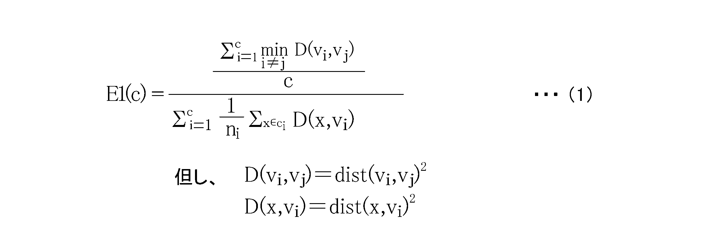
式(1)中の各値は、次の通りである。なお、i=1、2、・・・cである。また、クラスタ重心は、クラスタ内の各データの相加平均として求められる。図4には、データx、i番目のクラスタci、クラスタciの重心vi、クラスタ間距離dist(vi,vj)、クラスタ内距離dist(x、vi)の一例を模式的に示す。
n:クラスタリングの対象となるデータ数(全データ数)
x:データ
c:クラスタ数
ci:i番目のクラスタ
ni:クラスタciのデータ数
vi:クラスタciの重心(クラスタ重心)
D(x、vi):クラスタci内のデータxについてのクラスタ内距離指標値
D(vi,vj): クラスタciと他のクラスタcjとのクラスタ間距離指標値
dist(x、vi):クラスタci内のクラスタ重心とデータxとの距離(クラスタ内距離)
dist(vi,vj):クラスタciと他のクラスタcjとのクラスタ重心間の距離(クラスタ間距離)
n:クラスタリングの対象となるデータ数(全データ数)
x:データ
c:クラスタ数
ci:i番目のクラスタ
ni:クラスタciのデータ数
vi:クラスタciの重心(クラスタ重心)
D(x、vi):クラスタci内のデータxについてのクラスタ内距離指標値
D(vi,vj): クラスタciと他のクラスタcjとのクラスタ間距離指標値
dist(x、vi):クラスタci内のクラスタ重心とデータxとの距離(クラスタ内距離)
dist(vi,vj):クラスタciと他のクラスタcjとのクラスタ重心間の距離(クラスタ間距離)
式(1)の右辺の分母は、クラスタ内におけるデータの分散(データ同士の類似)の程度を全クラスタについて示す内的結合度になっている。クラスタ内距離指標値(=D(x、vi))は、クラスタ内に設定される距離の基点としての第1の代表点とクラスタ内のデータとの距離の程度(隔たりの大きさ)を示すものであり、クラスタ内の各々のデータについて求められる。この例では、第1の代表点をクラスタ重心とし、このクラスタ重心とデータとの距離であるクラスタ内距離(=dist(x、vi))の二乗の値をクラスタ内距離指標値にしている。
内的結合度は、クラスタごとの第1の指標値を当該クラスタ内のデータ数で除することで規格化した値の各クラスタについての総和として求められる。各クラスタの第1の指標値は、対応するクラスタ内のデータの分散の程度を示しており、この例では、対応するクラスタ内の各データについてのクラスタ内距離指標値の和である。
式(1)の右辺の分子は、クラスタの分離の程度を全クラスタについて示す外的分離度になっている。クラスタ間距離指標値(=D(vi,vj))は、1のクラスタと他の1のクラスタとの間の距離の程度を示しており、この例ではクラスタ間の距離の基点となる各クラスタの第2の代表点をクラスタ重心として、1のクラスタと他の1のクラスタとのクラスタ重心間の距離であるクラスタ間距離(=dist(vi,vj))の二乗の値である。
外的分離度は、クラスタごとの第2の指標値の各クラスタについての総和をクラスタ数で除して規格化した値である。第2の指標値は、1のクラスタと他の各クラスタとの分離の程度、すなわち当該1のクラスタについてのクラスタ間の距離の指標となる値であり、この例では、各々のクラスタについてのクラスタ間距離指標値の最小値である。
また、この例では、クラスタ内距離、クラスタ間距離をいずれもユークリッド距離としている。2つのq次元ベクトルであるデータをそれぞれa(a1,a2,・・・aq)、b(b1,b2,・・・bq)とすると、aとbとのユークリッド距離は、式(A)のように表される。

評価値E1(c)では、上記のように、外的分離度は、クラスタごとのクラスタの分離の程度の指標となる第2の指標値の各クラスタについての総和をクラスタ数で規格化した値であり、内的結合度は、クラスタごとのクラスタ内の各データの分散の程度を示す第1の指標値をクラスタ内のデータ数で規格化した値の各クラスタについての総和である。このため、全データ内において、他のデータのまとまりに対して、範囲の大きなデータのまとまりがある場合やデータの分布密度が高いデータのまとまりがある場合等であっても、個々のクラスタ内におけるデータの分散の程度が内的結合度に適正に反映される。すなわち、過剰な分類がされた場合に、評価値E1(c)がより大きくなるようなことがなく過剰な分類が抑制される。
評価値E1(c)は、クラスタリング状態が良好であれば、その程度に応じて値が大きくなる。したがって、評価値E1(c)が、極大値または最大値をとるようにクラスタ数cを決めればよい。なお、式(1)の右辺の逆数を評価値E1(c)とする場合には、評価値E1(c)が、極小値または最小値をとるようにクラスタ数cを決めればよい。また、クラスタ重心やクラスタ間距離は、k-means法の演算過程の途中結果を用いることができ演算数の削減に有利である。
上記評価値E1(c)では、クラスタ間の距離の指標である第2の指標値をクラスタ間距離指標値を用いて求めているが、式(2)に示す評価値E2(c)のように、予め設定された基準点からのクラスタまでの距離の程度を示す基準点クラスタ間距離指標値を用いて求めた値を第2の指標値とすることができる。評価値E2(c)は、詳細を後述するように、それを求める際の演算数が評価値E1(c)に比べて少なくなる。
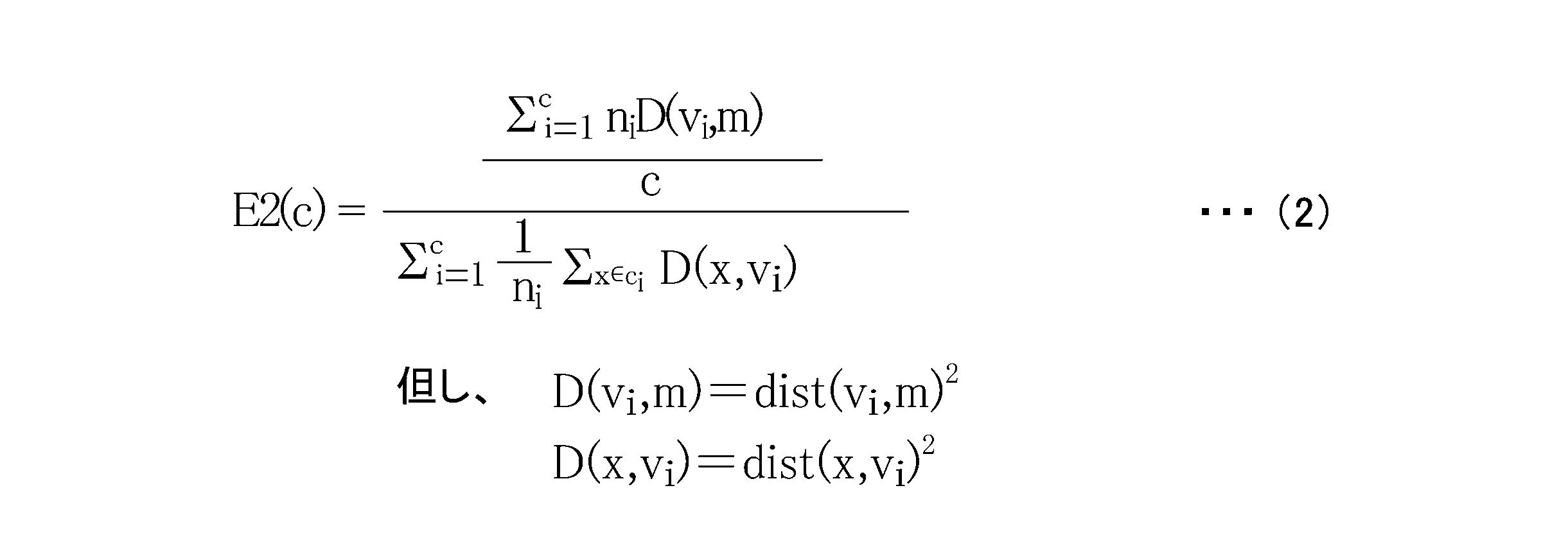
式(2)中の各値は、次の通りである。なお、その他の値は、式(1)のものと同じである、また、この例では、基準点をクラスタリングの対象となるn個の全データの重心としている。図5には、データx、i番目のクラスタci、クラスタciの重心vi、基準点クラスタ間距離dist(vi,m)、クラスタ内距離dist(x、vi)の一例を模式的に示す。
m:基準点
D(vi,m):クラスタciの基準点クラスタ間距離指標値
dist(vi,m):クラスタciのクラスタ重心と基準点との距離(基準点クラスタ間距離)
m:基準点
D(vi,m):クラスタciの基準点クラスタ間距離指標値
dist(vi,m):クラスタciのクラスタ重心と基準点との距離(基準点クラスタ間距離)
上記式(2)は、評価値E1(c)の式(1)と同じく、その右辺の分子が外的分離度であり、右辺の分母が内的結合度である。評価値E2(c)の外的分離度は、第2の指標値の各クラスタにつての総和であるが、基準点クラスタ間距離指標値をクラスタ内のデータ数で重み付けした値を第2の指標値としている。基準点クラスタ間距離指標値は、この例では、クラスタリング対象となるn個の全データの重心(以下、データ重心という)を基準点とし、基準点に対するクラスタリング側の距離の基点となる第2の代表点をクラスタ重心として、基準点とクラスタ重心との距離である基準点クラスタ間距離(=dist(vi,m))の二乗の値を基準点クラスタ間距離指標値としている。なお、基準点クラスタ間距離指標値に重み付けをする場合、重み付けする値は、クラスタ内のデータ数に限定されず、クラスタ内のデータ数に基づく値で重み付けしてもよい。
上記の評価値E2(c)においても、評価値E1(c)と同様に、外的分離度が、クラスタ間の距離の指標となるクラスタごとの第2の指標値の各クラスタについての総和をクラスタ数で規格化した値であり、内的結合度が、クラスタごとのクラスタ内の各データの分散の程度を示す第1の指標値をクラスタ内のデータ数で規格化した値の各クラスタについての総和になっているから、過剰な分類がされた場合に、評価値E2(c)がより大きくなるようなことがなく過剰な分類が抑制される。
評価値E2(c)は、評価値E1(c)と同じく、クラスタリング状態が良好であれば、その程度に応じて値が大きくなる。したがって、評価値E2(c)が、極大値または最大値をとるようにクラスタ数cを決めればよい。なお、式(2)の右辺の逆数を評価値E2(c)とする場合には、評価値E2(c)が、極小値または最小値をとるようにクラスタ数cを決めればよい。
なお、上記の評価値E1(c)、評価値E2(c)のように、クラスタ内距離指標値、クラスタ間距離指標値、基準点クラスタ間距離指標値として、対応するユークリッド距離(クラスタ内距離、クラスタ間距離、基準点クラスタ間距離)を二乗した値を用いる他に、対応するユークリッド距離そのものを用いることもできる。上記の例のように、対応するユークリッド距離を二乗した値を用いる場合には、ユークリッド距離そのものを用いるよりも、計算量を少なくすることができるという利点がある。
上記評価値E1(c)及び評価値E2(c)におけるクラスタ内距離、クラスタ間距離、基準点クラスタ間距離は、ユークリッド距離に限定されない。例えば、式(B)に示すマンハッタン距離や式(C)に示すミンコフスキー距離であってもよい。なお、式(C)におけるpは1以上の任意の値であるが、周知のようにp=1のときはマンハッタン距離に、p=2のときはユークリッド距離と同義である。また、この他にも「Point symmetry distance」等を用いてもよい。


さらに、評価値E1(c)、評価値E2(c)では、クラスタ内の各データについてのクラスタ内距離の基点である第1の代表点、クラスタ間距離の各クラスタの基点または基準点クラスタ間距離のクラスタ側の基点である第2の代表点をいずれもクラスタ重心にしているが、これに限定されない。例えば、第1の代表点、第2の代表点を各クラスタ内において、クラスタ重心に最も近いデータとしてもよい。また、第2の代表点は、クラスタ同士または基準点とクラスタとの離れた具合(距離)を測る上での基点であるから、隣接したクラスタあるいは基準点に最も近いまたは最も離れたクラスタ内のデータ等としてもよい。さらに、第1の代表点及び第2の代表点を、別途定めた基準によって決まるクラスタ内の点またはデータやクラスタ内の任意の点またはデータとしてもよい。
式(2)の基準点は、任意の点やデータに設定することができ、上記のようなデータ重心の他に、データ重心に最も近いデータ、いずれかのクラスタの第2の代表点、外部より指定する点やデータ、外部から指定された記憶装置のアドレスに格納されているデータ、最初に入力されたデータ等のように別途定めた基準によって決まる点やデータにしてもよい。
また、評価値E1(c)、評価値E2(c)では、内的結合度を求める際に、第1の指標値を、第1の値としての当該クラスタのデータ数niで規格化しているが、規格化するための第1の値は、これに限定されるものではなく、当該クラスタのデータ数niに基づく値とすることができる。例えば、当該クラスタのデータ数niの冪(ni
2、ni
3、ni
1/2、ni
-2等)、データ数niを定数倍した値、データ数niに一定数を減算または加算した値、データ数niとクラスタ数cとを予め決めた関数F(ni,c)、例えば「F(ni,c)=ni-c」、kを定数とした「F(ni,c)=k・ni-c」等に適用した結果等を第1の値として用いることができる。
また、外的分離度を求める際に、第2の値としてのクラスタ数cで規格化しているが、第2の値は、これに限定されるものではなく、クラスタ数cに基づく値で規格化することができる。クラスタ数c以外のクラスタ数に基づく値としては、第1の値と同様に、例えば、クラスタ数cの冪、クラスタ数cを定数倍した値、クラスタ数cに一定数を減算または加算した値、クラスタ数cと全データ数nとを予め決めた関数G(n,c)に適用した結果等を第2の値として用いることができる。
上記では、評価値E1(c)、評価値E2(c)は、評価値を求める演算を内的結合度と外的分離度との比とするものであるが、評価値を求める演算はこれに限定されない。上記のように求められる内的結合度は、その値が小さいほど、クラスタ内のデータ相互の類似性が高くなるように各クラスタ内のデータがまとまったクラスタリング状態となることを意味する。一方で、上記のように求められる外的分離度は、その値が大きいほど、クラスタ相互間の類似性が低くなるように各クラスタが相互に離れたクラスタリング状態となることを意味する。このため、内的結合度と外的分離度とから評価値を求める演算は、内的結合度が小さくなる方向に変化したとき、また外的分離度が大きくなる方向に変化したときに、評価値が増加または減少の一方に変化するようにすればよく、そのような結果が得られる内的結合度と外的分離度とを変数とする演算式を用いればよい。
評価値を求める演算としては、上述のように内的結合度と外的分離度との比とするものの他に、例えば、次の各式に示すように、内的結合度と外的分離度の一方の逆数と他方とをそれぞれ重み付けして加算することで評価値Eを求めるもの、内的結合度と外的分離度の一方から他方をそれぞれ重み付けして減算することで評価値Eを求めるもの等を用いることができる。なお、式中の値Compは内的結合度を、Sepは外的分離度を、Wa、Wbは重み付けの定数であり、Wa,Wb≠0である。
E=Wb・Sep+Wa・(1/Comp)
E=Wb・(1/Sep)+Wa・Comp
E=Wb・Sep-Wa・Comp
E=Wa・Comp-Wb・Sep
E=Wb・Sep+Wa・(1/Comp)
E=Wb・(1/Sep)+Wa・Comp
E=Wb・Sep-Wa・Comp
E=Wa・Comp-Wb・Sep
以下、サンプルのデータをクラスタリングし、評価値E1(c)、評価値E2(c)を用いて最適なクラスタ数を決定した実施例1、2について説明する。実施例1、2では、クラスタリング手法としてk-means法を用い、最適なクラスタ数の決定の手順としては、図3に示すものを用いて評価値が最大となるものとした。クラスタリング数の範囲は、2~10とした。また、比較例1として、同様な条件の下で、非特許文献1に記載された評価値VRC(c)を用いて最適なクラスタ数を決定した。
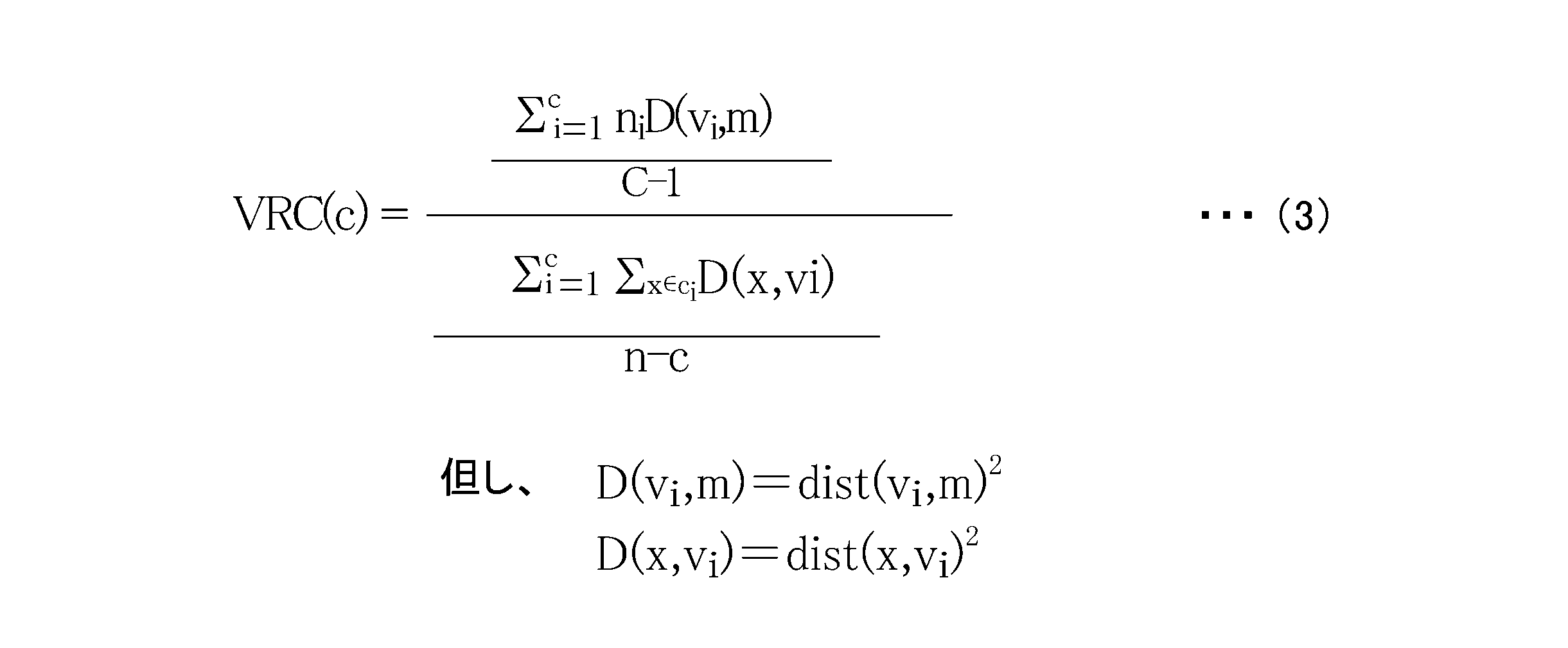
評価値VRC(c)の算出式を式(3)に示す。なお、式(3)の各値は、式(1)または式(2)のもとの同じである。評価値VRC(c)では、式(6)の分母の値が内的結合度を示しており、分子の値が外的分離度を示している。
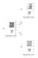
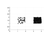
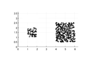
実施例1、2及び比較例1では、図6(a)に示すサンプル1、図7に示すサンプル2、図8に示すサンプル3に対してクラスタリングを実施した。これら図6(a)、図7、図8は、いずれも2次元ベクトルのデータの分布状態を示している。
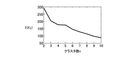
サンプル1では、データが互いに離れた小領域と、この小領域よりもサイズが大きい大領域にそれぞれ同じ密度で分布させている。小領域のデータ数は、100個、大領域のデータ数は、400個であり、大領域は、小領域の4倍の面積である。このサンプル1について、クラスタ数cを2~10の範囲で変化させてクラスタリングした場合の評価値E1(c)、評価値E2(c)及び評価値VRC(c)の変化を図9ないし図11にそれぞれ示す。
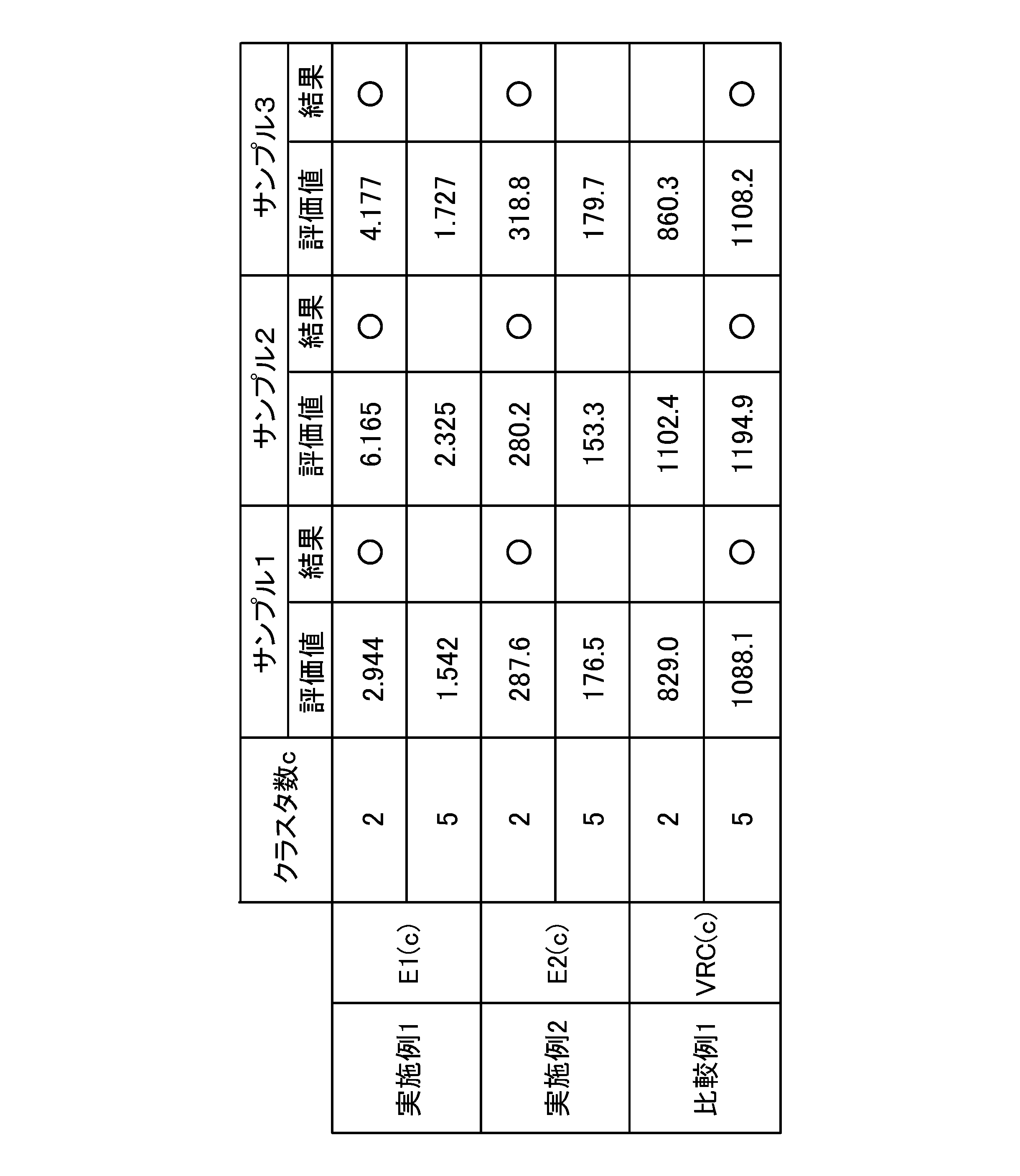
評価値E1(c)、評価値E2(c)のいずれの場合にも、クラスタ数cが「2」のときに評価値が最大となり、そのときのクラスタリングの状態は、図6(b)に示すようなものになり、小領域のデータと大領域のデータとがそれぞれ1つのクラスタに分類される結果となった。この結果は、サンプル1のデータの分布に対する人間の感覚的な判断と一致している。一方、評価値VRC(c)では、クラスタ数cが「5」のときに評価値が最大となり、そのときのクラスタリングの状態は、図6(c)に示すように、小領域のデータが1つのクラスタに分類され、大領域のデータは4つのクラスタに分類される結果になった。なお、クラスタリング手法として同じ手法を用いているため、クラスタ数cが同じであれば、評価値E1(c)、評価値E2(c)、評価値VRC(c)のいずれにおいてもクラスタリングの状態は同じである。
上記同様にして、サンプル2についての評価値E1(c)、評価値E2(c)、評価値VRC(c)の変化を調べた結果を図12ないし図14に、またサンプル3についての評価値E1(c)、評価値E2(c)、評価値VRC(c)の変化を調べた結果を図15ないし図17にそれぞれ示す。
サンプル2は、互いに離れた同じサイズの低密度領域と高密度領域にデータを分布させたものであり、低密度領域よりも高密度領域のデータの密度が高くなっている。サンプル2では、低密度領域のデータ数が50個であり、高密度領域のデータ数が500個である。サンプル3では、互いに離れた小領域とこの小領域よりもサイズが大きい大領域とに、異なる密度でデータを分布させたものであり、小領域よりも大領域のデータの密度が高くなっている。サンプル3では、データ数は、小領域が50個、大領域が400個であり、大領域は、小領域の4倍の面積である。
評価値E1(c)、E2(c)は、上記サンプル2、サンプル3についても、サンプル1と同じく、クラスタ数cが「2」のときに最大となり、サンプル2、3の領域ごとにそれらのデータが1つのクラスタに分類される結果となった。一方、評価値VRC(c)は、サンプル2、サンプル3についても、クラスタ数cが「5」のときに最大となり、サンプル2の低密度領域、サンプル3の小領域のデータがそれぞれ1つのクラスタに分類され、サンプル2の高密度領域、サンプル3の大領域のデータがそれぞれ4つのクラスタに分類された。
表1に、サンプル1~3についてのクラスタ数cが「2」と「5」の場合の各評価値の値を示す。なお、最大値となった評価値に対して表1中の「結果」の欄に丸印を付してある。
また、表2には、サンプル1について、クラスタ数cが「2」、「5」各場合の評価値E2(c)、VRC(c)における内的結合度及び外的分離度の詳細を示す。クラスタ数cが「5」のときの評価値E2(c)における内的結合度は、クラスタ数cが「2」のときのものに比べて僅かに小さな値になっているが、クラスタ数cが「5」のときの評価値VRC(c)における内的結合度は、クラスタ数cが「2」のものに比べて1/3以下の値であり、かなり小さな値になっている。
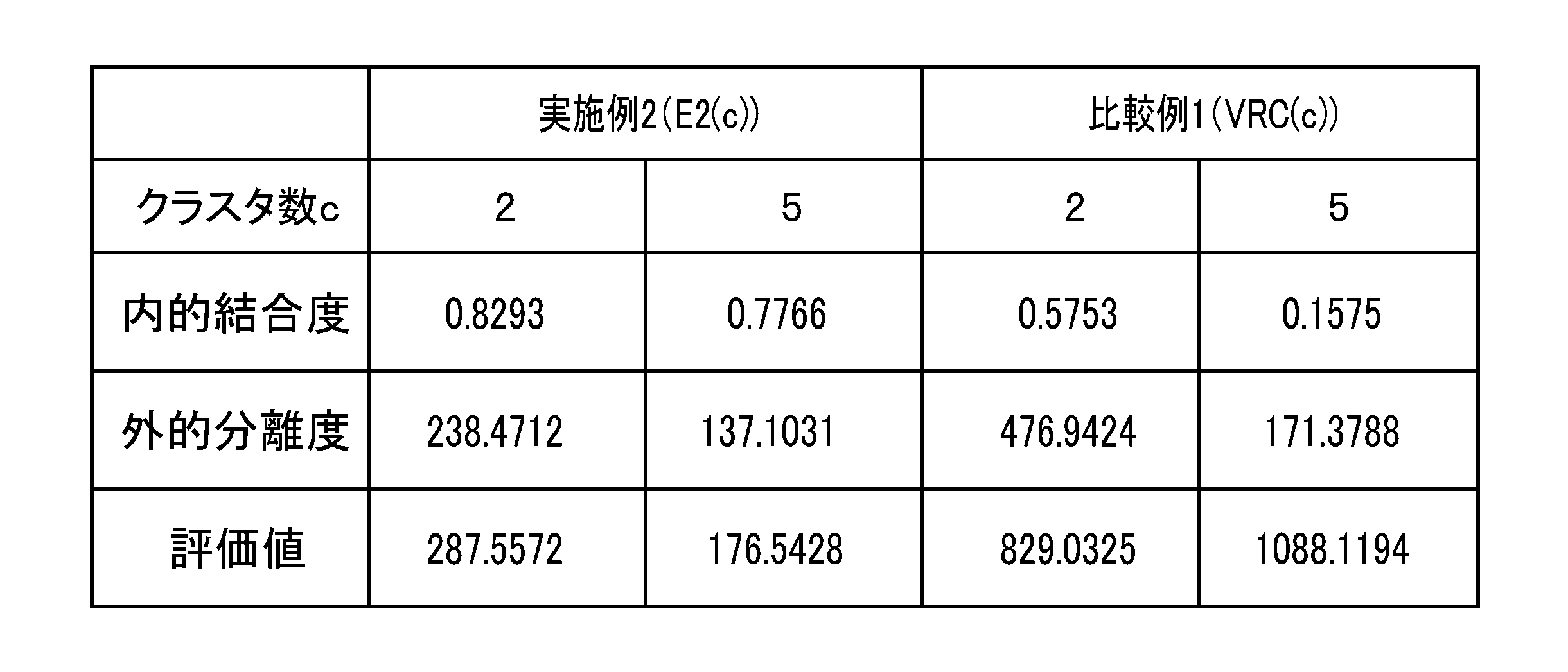
上述のように評価値E2(c)は、クラスタごとのクラスタ内距離指標値の和、すなわちクラスタごとの第1の指標値を、当該クラスタ内のデータ数niで除して規格化した値の各クラスタについての総和を内的結合度にしている。一方、評価値VRC(c)の内的結合度は、上記式(3)から分かるように、クラスタごとに求めた第1の指標値の各クラスタについての総和を「n-c(=全データ数-クラスタ数)」で除して規格化した値である。なお、全データ数nに対してクラスタ数cの変化量ないし値を無視しても問題ないので、便宜上、全データ数nで除して規格化しているものとして説明する。
上述のように、サンプル1は、クラスタ数cが「2」のときには、小領域のデータと大領域のデータとがそれぞれ1つのクラスタに分類され(図6(b))、クラスタ数cが「5」のときには、小領域のデータが1つのクラスタに分類され、大領域のデータは4つのクラスタに分類される(図6(c))。クラスタ数cが「2」のときに比べて、クラスタ数cが「5」ときには、大領域のデータは4つのクラスタに分類されることにともない、それら4個のクラスタ内の各データについてのクラスタ内距離指標値がかなり小さくなる。この結果、それら4個のクラスタのそれぞれについての第1の指標値(=クラスタ内距離指標値の和)もかなり小さくなり、第1の指標値の各クラスタについての総和もかなり小さくなる。
評価値VRC(c)の内的結合度は、第1の指標値の各クラスタについての総和を全データ数nで規格化した値であり、全データ数nは変化しない値である。したがって、クラスタ数cが大きくなって第1の指標値の総和がかなり小さくなると、それに応じて内的結合度もかなり小さくなる。このため、クラスタ数cが「5」のときの評価値VRC(c)における内的結合度は、クラスタ数cが「2」のものに比べて1/3以下の値になっている。
上記のようにクラスタ数cが大きくなることによって、第1の指標値がかなり小さくなる点については、評価値E2(c)を求める場合においても全く同じである。しかしながら、評価値E2(c)では、上記のように、クラスタごとの第1の指標値を当該クラスタ内のデータ数niで除して規格化しており、そのデータ数niは、クラスタの範囲が狭くなることによって小さな値になる。したがって、クラスタ数cが大きくなることによって第1の指標値が小さくなっても、内的結合度の変化は小さい。このため、上記のようにクラスタ数cが「5」のときの評価値E2(c)における内的結合度は、クラスタ数cが「2」のものに比べて僅かな減少になっている。
クラスタ数の増減にともなう外的分離度の変化によっても、評価値E2(c)、評価値VRC(c)は変化するが、サンプル1のようなデータの分布については、評価値VRC(c)では、上記のようにクラスタ数cが増大したときに内的結合度が大きく減少する傾向により、クラスタ数cが「5」のときに、その値が最も高くなり、人間の感覚的な判断よりも過剰に分類された結果になったと考えられる。これに対して、評価値E2(c)では、クラスタ数cが増大したときに内的結合度が大きく減少する傾向がないため、クラスタ数cが「2」のときに最も高くなり、過剰な分類が抑制されて人間の感覚的な判断と一致した結果になったと考えられる。なお、他のサンプル2、3についてもサンプル1と同様であり、評価値E1(c)についても評価値E2(c)と同様である。
また、図18に示すサンプルA~Eについて、実施例3、比較例2、3を実施した。実施例3では評価値E1(c)を、比較例2では評価値VRC(c)を、比較例3では、既知のDBインデックス(以下、評価値DB(c)と称する)をそれぞれ用いて、最適なクラスタ数を調べた。サンプルA~EのうちサンプルBは、データが三次元ベクトルであり、その他はデータが二次元ベクトルである。評価値DB(c)は、式(4)で求められる。
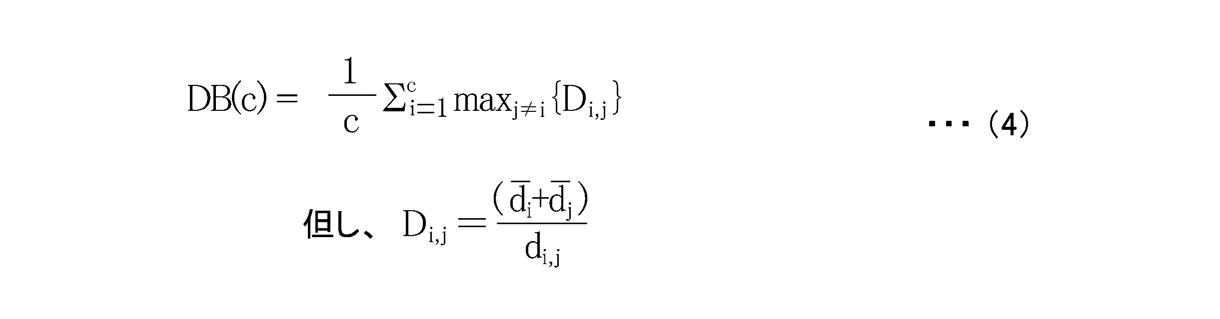
式(4)中の各値は、次の通りである。
di(上にバ-):i番目のクラスタにおけるクラスタ内距離の平均値
dj(上にバ-):j番目のクラスタにおけるクラスタ内距離の平均値
di,j:i番目とj番目の各クラスタの重心間の距離(クラスタ間距離)
di(上にバ-):i番目のクラスタにおけるクラスタ内距離の平均値
dj(上にバ-):j番目のクラスタにおけるクラスタ内距離の平均値
di,j:i番目とj番目の各クラスタの重心間の距離(クラスタ間距離)
上述のように、評価値E1(c)、E2(c)では、クラスタ内の各データの分散の程度を示す各々のクラスタについての第1の指標値をクラスタのデータ数に基づく第1の値で規格化した値の総和を内的結合度とし、クラスタ間の距離の指標となる各々のクラスタについての第2の指標値の総和をクラスタ数に基づく第2の値で規格化した値を外的分離度としており、評価値E1(c)、E2(c)は、それら内的結合度と外的分離度との比として求められる。これに対して、評価値DB(c)では、一のクラスタを含む一対のクラスタに関してクラスタリング状態が最も悪いと評価される他の一のクラスタとの組み合わせにおける各クラスタ内のデータ分散の程度と当該一のクラスタ及び当該の他の一のクラスタの分離の程度との比を各クラスタについてそれぞれ求め、評価値DB(c)は、それら各クラスタの比の平均であり、評価値E1(c)、E2(c)とは異なる。
各評価値を用いて判別された最適なクラスタ数の結果を表3に示す。なお、評価値E1(c)、評価値VRC(c)については、それらが最大値となるクラスタ数を最適なクラスタ数とし、評価値DB(c)は、それが最小値となるクラスタ数を最適なクラスタ数とした。

実施例3では、サンプルA~Eのいずれにおいても、クラスタリング数を含むクラスタリングの結果が人間の感覚的な判断と一致した結果となった。これに対して、比較例2は、サンプルC~Eにおいて、人間の感覚的な判断によるクラスタ数と比較してクラスタ数が多くなり過剰に分割される結果となった。また、比較例3では、人間の感覚的な判断と比較して、比較例2のように過剰な分割とはならなかったが、サンプルCにおいてクラスタリング数が少ない結果となった。すなわち、比較例3の評価値DB(c)は、データの複数のまとまりが相互に近接している場合には、それらをまとめて1つのクラスタに分類したときに値が高くなる傾向があることが分かる。
10 演算装置
11 評価値演算部
12 クラスタリング部
13 制御部
14 データ記憶部
E1(c) 評価値
E2(c) 評価値
11 評価値演算部
12 クラスタリング部
13 制御部
14 データ記憶部
E1(c) 評価値
E2(c) 評価値
Claims (11)
- 複数のデータをクラスタリングしたときのクラスタ数によるクラスタリング状態の評価値を演算装置で算出するクラスタリングの評価値算出方法において、
クラスタリングされたデータに関する情報を取得する取得ステップと、
取得した前記情報に基づいて前記評価値を算出する算出ステップと
を有し、
前記算出ステップは、
クラスタ内のデータの分散の程度を示す各々の前記クラスタについての第1の指標値を当該クラスタのデータ数に基づく第1の値で規格化した値の各前記クラスタの総和である内的結合度と、
前記クラスタ間の距離の指標となる各々の前記クラスタについての第2の指標値の総和を前記クラスタ数に基づく第2の値で規格化した外的分離度と
をそれぞれ求め、
前記内的結合度と前記外的分離度とを変数とする所定の演算式から前記評価値を算出する
ことを特徴とするクラスタリングの評価値算出方法。 - 各々の前記クラスタの前記第1の指標値は、当該クラスタ内の第1の代表点と当該クラスタ内の各データとの間のクラスタ内距離の和または二乗和であることを特徴とする請求項1に記載のクラスタリングの評価値算出方法。
- 前記第1の代表点は、前記クラスタ内のデータの重心であることを特徴とする請求項2に記載のクラスタリングの評価値算出方法。
- 前記第1の値は、前記クラスタ内のデータ数であることを特徴とする請求項1ないし3のいずれか1項に記載のクラスタリングの評価値算出方法。
- 各々の前記クラスタの前記第2の指標値は、当該クラスタ内の第2の代表点と他の前記クラスタ内の第2の代表点との間のクラスタ間距離のうち、最も小さい前記クラスタ間距離または最も小さい前記クラスタ間距離を二乗した値であることを特徴とする請求項1ないし4のいずれか1項に記載のクラスタリングの評価値算出方法。
- 各々の前記クラスタの前記第2の指標値は、全データの基準点と当該クラスタ内の第2の代表点との間の基準点クラスタ間距離または前記基準点クラスタ間距離を二乗した値であることを特徴とする請求項1ないし4のいずれか1項に記載のクラスタリングの評価値算出方法。
- 各々の前記クラスタの前記第2の指標値は、全データの基準点と当該クラスタ内の第2の代表点との間の基準点クラスタ間距離または前記基準点クラスタ間距離を二乗した値のいずれかに当該クラスタ内のデータ数に基づく重み付けをした値であることを特徴とする請求項1ないし4のいずれか1項に記載のクラスタリングの評価値算出方法。
- 前記基準点は、全データの重心であることを特徴とする請求項6または7に記載のクラスタリングの評価値算出方法。
- 前記第2の代表点は、前記クラスタ内のデータの重心であることを特徴とする請求項6ないし8のいずれか1項に記載のクラスタリングの評価値算出方法。
- 前記内的結合度と前記外的分離度との比を前記評価値として算出することを特徴とする請求項1ないし9のいずれか1項に記載のクラスタリングの評価値算出方法。
- 請求項1ないし10のいずれか1項に記載のクラスタリングの評価値算出方法を用いて、前記クラスタ数の異なるクラスタリングの結果に対する前記評価値をそれぞれ算出し、
各前記評価値のうちの極値、または最大値若しくは最小値の前記評価値に対応する前記クラスタ数を最適値として判定する
ことを特徴とするクラスタリング数決定方法。
Priority Applications (2)
| Application Number | Priority Date | Filing Date | Title |
|---|---|---|---|
| JP2019533991A JP7205908B2 (ja) | 2017-08-03 | 2018-07-05 | クラスタリングの評価値算出方法及びクラスタ数決定方法 |
| US16/634,512 US11610083B2 (en) | 2017-08-03 | 2018-07-05 | Method for calculating clustering evaluation value, and method for determining number of clusters |
Applications Claiming Priority (2)
| Application Number | Priority Date | Filing Date | Title |
|---|---|---|---|
| JP2017151146 | 2017-08-03 | ||
| JP2017-151146 | 2017-08-03 |
Publications (1)
| Publication Number | Publication Date |
|---|---|
| WO2019026523A1 true WO2019026523A1 (ja) | 2019-02-07 |
Family
ID=65233805
Family Applications (1)
| Application Number | Title | Priority Date | Filing Date |
|---|---|---|---|
| PCT/JP2018/025498 Ceased WO2019026523A1 (ja) | 2017-08-03 | 2018-07-05 | クラスタリングの評価値算出方法及びクラスタ数決定方法 |
Country Status (3)
| Country | Link |
|---|---|
| US (1) | US11610083B2 (ja) |
| JP (1) | JP7205908B2 (ja) |
| WO (1) | WO2019026523A1 (ja) |
Cited By (5)
| Publication number | Priority date | Publication date | Assignee | Title |
|---|---|---|---|---|
| WO2020189706A1 (ja) * | 2019-03-20 | 2020-09-24 | 株式会社日立産業制御ソリューションズ | クラスタ分割評価装置、クラスタ分割評価方法及びクラスタ分割評価プログラム |
| JP2021013048A (ja) * | 2019-07-03 | 2021-02-04 | 公立大学法人会津大学 | 3次元ネットワークオンチップによるスパイキングニューラルネットワーク |
| JP2021103398A (ja) * | 2019-12-25 | 2021-07-15 | 株式会社 日立産業制御ソリューションズ | クラスタ分割評価装置、クラスタ分割評価方法及びクラスタ分割評価プログラム |
| JP2022061690A (ja) * | 2020-10-07 | 2022-04-19 | 株式会社国際電気通信基礎技術研究所 | 学習用データ生成方法、信号種別分類システム、データ収集システム、および、プログラム |
| JP2022176899A (ja) * | 2021-05-17 | 2022-11-30 | 富士通株式会社 | 機械学習モデルを訓練するためのデータ要約 |
Families Citing this family (4)
| Publication number | Priority date | Publication date | Assignee | Title |
|---|---|---|---|---|
| WO2022067327A1 (en) * | 2020-09-25 | 2022-03-31 | Digital Realty Trust, Inc. | Pervasive data center architecture systems and methods |
| CN115311482B (zh) * | 2022-07-20 | 2025-10-21 | 西安电子科技大学杭州研究院 | 一种基于分离度的小样本半监督聚类方法 |
| CN117435900B (zh) * | 2023-11-10 | 2026-06-19 | 吉林大学 | 一种海洋可控源电磁数据质量评价方法 |
| CN118802615B (zh) * | 2024-07-02 | 2026-01-16 | 中国移动通信集团山西有限公司 | 专网质量评估方法、装置、设备、介质及计算机程序产品 |
Family Cites Families (9)
| Publication number | Priority date | Publication date | Assignee | Title |
|---|---|---|---|---|
| CA2785197A1 (en) * | 2009-12-23 | 2011-06-30 | The Governors Of The University Of Alberta | Automated, objective and optimized feature selection in chemometric modeling (cluster resolution) |
| WO2012055100A1 (en) * | 2010-10-27 | 2012-05-03 | Nokia Corporation | Method and apparatus for identifying a conversation in multiple strings |
| US8214365B1 (en) * | 2011-02-28 | 2012-07-03 | Symantec Corporation | Measuring confidence of file clustering and clustering based file classification |
| WO2017059250A1 (en) * | 2015-09-30 | 2017-04-06 | Hampton Creek, Inc. | Systems and methods for identifying entities that have a target property |
| US20170091270A1 (en) * | 2015-09-30 | 2017-03-30 | Linkedln Corporation | Organizational url enrichment |
| US10762439B2 (en) * | 2016-07-26 | 2020-09-01 | International Business Machines Corporation | Event clustering and classification with document embedding |
| CN107169417B (zh) * | 2017-04-17 | 2021-01-12 | 上海大学 | 基于多核增强和显著性融合的rgbd图像协同显著性检测方法 |
| CN107480694B (zh) * | 2017-07-06 | 2021-02-09 | 重庆邮电大学 | 基于Spark平台采用两次评价的加权选择集成三支聚类方法 |
| CN107368856B (zh) * | 2017-07-25 | 2021-10-19 | 深信服科技股份有限公司 | 恶意软件的聚类方法及装置、计算机装置及可读存储介质 |
-
2018
- 2018-07-05 US US16/634,512 patent/US11610083B2/en active Active
- 2018-07-05 JP JP2019533991A patent/JP7205908B2/ja active Active
- 2018-07-05 WO PCT/JP2018/025498 patent/WO2019026523A1/ja not_active Ceased
Non-Patent Citations (2)
| Title |
|---|
| ARBELAITZ, OLATZ ET AL.: "An extensive comparative study of cluster validity indices", PATTERN RECOGNITION, vol. 46, no. 1, January 2013 (2013-01-01), pages 243 - 256, XP055571755 * |
| SAITTA, S. ET AL.: "A comprehensive validity index for clustering", INTELLIGENT DATA ANALYSIS, vol. 12, no. 6, 2008, pages 529 - 548, XP055571762 * |
Cited By (10)
| Publication number | Priority date | Publication date | Assignee | Title |
|---|---|---|---|---|
| WO2020189706A1 (ja) * | 2019-03-20 | 2020-09-24 | 株式会社日立産業制御ソリューションズ | クラスタ分割評価装置、クラスタ分割評価方法及びクラスタ分割評価プログラム |
| JP2020154825A (ja) * | 2019-03-20 | 2020-09-24 | 株式会社 日立産業制御ソリューションズ | クラスタ分割評価装置、クラスタ分割評価方法及びクラスタ分割評価プログラム |
| CN113557538A (zh) * | 2019-03-20 | 2021-10-26 | 日立产业控制解决方案有限公司 | 聚类分割评价装置、聚类分割评价方法以及聚类分割评价程序 |
| JP2021013048A (ja) * | 2019-07-03 | 2021-02-04 | 公立大学法人会津大学 | 3次元ネットワークオンチップによるスパイキングニューラルネットワーク |
| JP7277682B2 (ja) | 2019-07-03 | 2023-05-19 | 公立大学法人会津大学 | 3次元ネットワークオンチップによるスパイキングニューラルネットワーク |
| JP2021103398A (ja) * | 2019-12-25 | 2021-07-15 | 株式会社 日立産業制御ソリューションズ | クラスタ分割評価装置、クラスタ分割評価方法及びクラスタ分割評価プログラム |
| JP2022061690A (ja) * | 2020-10-07 | 2022-04-19 | 株式会社国際電気通信基礎技術研究所 | 学習用データ生成方法、信号種別分類システム、データ収集システム、および、プログラム |
| JP7557861B2 (ja) | 2020-10-07 | 2024-09-30 | 株式会社国際電気通信基礎技術研究所 | 学習用データ生成方法、信号種別分類システム、データ収集システム、および、プログラム |
| JP2022176899A (ja) * | 2021-05-17 | 2022-11-30 | 富士通株式会社 | 機械学習モデルを訓練するためのデータ要約 |
| JP7800288B2 (ja) | 2021-05-17 | 2026-01-16 | 富士通株式会社 | 機械学習モデルを訓練するためのデータ要約 |
Also Published As
| Publication number | Publication date |
|---|---|
| JP7205908B2 (ja) | 2023-01-17 |
| US11610083B2 (en) | 2023-03-21 |
| US20200272861A1 (en) | 2020-08-27 |
| JPWO2019026523A1 (ja) | 2020-09-10 |
Similar Documents
| Publication | Publication Date | Title |
|---|---|---|
| JP7205908B2 (ja) | クラスタリングの評価値算出方法及びクラスタ数決定方法 | |
| CN113075129B (zh) | 一种基于近邻子空间划分高光谱影像波段选择方法及系统 | |
| CN105488809B (zh) | 基于rgbd描述符的室内场景语义分割方法 | |
| Meesrikamolkul et al. | Shape-based clustering for time series data | |
| JP5792747B2 (ja) | テキスト分類の方法及びシステム | |
| Zhou et al. | A novel internal validity index based on the cluster centre and the nearest neighbour cluster | |
| Reza et al. | ICA and PCA integrated feature extraction for classification | |
| Wang et al. | CLUES: A non-parametric clustering method based on local shrinking | |
| CN109871768B (zh) | 基于共享最近邻的高光谱最优波段选择方法 | |
| WO2018001384A1 (zh) | 数据处理、数据识别方法和装置、计算机设备 | |
| CN103914705B (zh) | 一种基于多目标免疫克隆的高光谱图像分类和波段选择的方法 | |
| CN106971091B (zh) | 一种基于确定性粒子群优化和支持向量机的肿瘤识别方法 | |
| CN103295014B (zh) | 基于像素位置排列直方图的图像局部特征描述方法 | |
| CN113222027A (zh) | 基于加权共享最近邻的自适应聚类中心密度峰值聚类算法 | |
| Gao et al. | James–stein shrinkage to improve k-means cluster analysis | |
| CN111791090A (zh) | 一种基于边缘计算与粒子群算法的刀具寿命磨损判定方法 | |
| Li et al. | On the implicit assumptions of gans | |
| TW201621754A (zh) | 多類別物件分類方法及系統 | |
| CN108921853B (zh) | 基于超像素和免疫稀疏谱聚类的图像分割方法 | |
| CN107704872A (zh) | 一种基于相对最离散维分割的K‑means聚类初始中心选取方法 | |
| JP2017129990A (ja) | 画像認識装置、画像認識方法、及び画像認識プログラム | |
| CN111027609B (zh) | 一种图像数据加权分类方法和系统 | |
| CN104504305B (zh) | 监督基因表达数据分类方法 | |
| CN110580498A (zh) | 一种数据采样方法及装置 | |
| EP2890043B1 (en) | Space division method, space division device, and space division program |
Legal Events
| Date | Code | Title | Description |
|---|---|---|---|
| DPE1 | Request for preliminary examination filed after expiration of 19th month from priority date (pct application filed from 20040101) | ||
| ENP | Entry into the national phase |
Ref document number: 2019533991 Country of ref document: JP Kind code of ref document: A |
|
| NENP | Non-entry into the national phase |
Ref country code: DE |
|
| 122 | Ep: pct application non-entry in european phase |
Ref document number: 18842310 Country of ref document: EP Kind code of ref document: A1 |