WO2019003644A1 - 希少事象解析装置、希少事象解析方法および希少事象解析プログラム記録媒体 - Google Patents
希少事象解析装置、希少事象解析方法および希少事象解析プログラム記録媒体 Download PDFInfo
- Publication number
- WO2019003644A1 WO2019003644A1 PCT/JP2018/017755 JP2018017755W WO2019003644A1 WO 2019003644 A1 WO2019003644 A1 WO 2019003644A1 JP 2018017755 W JP2018017755 W JP 2018017755W WO 2019003644 A1 WO2019003644 A1 WO 2019003644A1
- Authority
- WO
- WIPO (PCT)
- Prior art keywords
- parameters
- histogram
- class
- past
- parameter
- Prior art date
- Legal status (The legal status is an assumption and is not a legal conclusion. Google has not performed a legal analysis and makes no representation as to the accuracy of the status listed.)
- Ceased
Links
Images






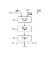


Classifications
-
- G—PHYSICS
- G06—COMPUTING OR CALCULATING; COUNTING
- G06F—ELECTRIC DIGITAL DATA PROCESSING
- G06F30/00—Computer-aided design [CAD]
Definitions
- the present invention relates to a rare event analysis device, a rare event analysis method, and a rare event analysis program recording medium.
- stray light is light that arises potentially in optical design and is caused by a rare incoherent ray that does not follow the design light path. That is, a light beam coming into the light receiving surface in an irregular path (optical path) is called stray light, which causes a decrease in image contrast and noise.
- Patent Document 1 splits one light beam into a transmitted light beam and a reflected light beam, and enables tracking of stray light by tracking both light beams, thereby achieving an "optical simulation apparatus" based on a more accurate light ray tracing method. Is realized.
- Patent Document 1 does not suggest or disclose at all a device for determining a combination of parameters (events) to be input to an optical simulation apparatus in order to efficiently detect a rare event of stray light.
- An object of the present invention is to provide a rare event analysis device, a rare event analysis method, and a rare event analysis program recording medium, which solve the problems described above.
- the rare event analyzer is a rare event analyzer for discovering the possibility of occurrence of a rare event, and N in each test k (1 ⁇ k ⁇ K) based on the proposed distribution Q (X).
- An evaluation function that determines N parameters X k each defining an event, which is used for the simulation of one cycle, and sequentially defines the possibility of the rare event occurring one by one the N parameters X k
- a parameter determination unit that supplies a simulator having C (X); and an evaluation value acquisition unit that acquires N evaluation values C (X k ) output from the simulator corresponding to the N parameters X k.
- the parameter determination unit includes N past parameters X k-1 used for N simulations of the past test (k-1) and the N past parameters X k-1 N times against N parameters X k to be used for N simulations in the current test k are determined based on the N past evaluation values C (X k-1 ) acquired in the simulation, and the parameter determination The part inputs the N past parameters X k-1 and the N past evaluation values C (X k-1 ), sets the evaluation value as a class, and counts the number of parameters of each class A histogram calculation unit for calculating a histogram to be; and a distribution of random numbers for generating N parameters X k used for N simulations in the current test k based on the calculated histogram.
- Histo frequency parameters of the threshold value C th or more of each class defined with respect to classes is such that more than the frequency of the parameters in the threshold C th following each class
- the random number distribution definition section for defining; based on the distribution of random numbers the definition, a parameter generating unit that generates the parameters X k to be used for each simulation in the present study k ;
- the rare event analysis method of the present invention is a rare event analysis method for finding out the possibility of occurrence of a rare event, and N in each test k (1 ⁇ k ⁇ K) based on the proposed distribution Q (X).
- An evaluation function that determines N parameters X k each defining an event, which is used for the simulation of one cycle, and sequentially defines the possibility of the rare event occurring one by one the N parameters X k Determining a parameter to be supplied to a simulator having C (X); and obtaining N evaluation values C (X k ) output from the simulator corresponding to the N parameters X k
- determining the parameters includes N past parameters X k-1 used for N simulations of the past test (k-1), and the N past parameters X k N for -1 N parameters X k to be used for N simulations in the current test k are determined based on N past evaluation values C (X k-1 ) obtained in The determination of the parameters may be performed by inputting the N past parameters X k-1 and the N
- the rare event analysis program recording medium of the present invention is a recording medium recording a rare event analysis program for finding out the possibility of occurrence of a rare event in a computer, wherein the rare event analysis program is proposed distribution in the computer Based on Q (X), determine N parameters X k each defining an event to be used for N simulations in each test k (1 ⁇ k ⁇ K), and determine the N parameters
- a parameter determination procedure for supplying to a simulator having an evaluation function C (X) which defines the possibility of occurrence of the rare event sequentially one by one X k ; and the simulator corresponding to the N parameters X k an evaluation value obtaining step of obtaining the output is the N evaluation value C (X k) from; to execute the said parameter determination procedure, the computer, in the past Test (k-1) and N times the simulation of N past parameters X k-1 used in the of the N pieces of past parameters X k-1 of N past acquired in N times of simulation for The N parameters X k to be used for N simulations in the current test
- FIG. 7 is a diagram showing an example of a histogram showing sampled events on a fatal degree (evaluation function) C (X) in the multicanonical MCMC method. It is a figure for explaining the Multicanonical MCMC method specialized for rare event search.
- FIG. 7 is a diagram showing an example of a histogram showing sampled events on a fatal degree (evaluation function) C (X) in the multicanonical MCMC method. It is a figure for explaining the Multicanonical MCMC method specialized for rare event search.
- FIG. 7 shows a comparison of the number of rays obtained that cause stray light to the number of histogram updates between the standard Multicanonical MCMC method (sm-MCMC) and the proposed Focused Multicanonical MCMC method (fm-MCMC) .
- FIG. 1 is a block diagram showing an optical system design support system according to a first embodiment of the present invention. It is a block diagram which shows in detail the structure of the parameter determination part used in the optical system design support system shown in FIG. It is a block diagram showing the optical system design support system by a 2nd example of the present invention. It is a block diagram which shows in detail the structure of the parameter determination part used for the optical system design support system shown in FIG. It is a block which shows the rare event analyzer according to the 3rd Example of this invention. It is a block diagram which shows the structure of the parameter determination part used for the rare event analyzer shown in FIG. 12 in detail.
- Markov chain Monte Carlo methods is a general term for an algorithm for sampling a probability distribution based on creating a Markov chain having the probability distribution to be determined as an equilibrium distribution.
- the MCMC method is a method combining "Markov chain” and "Monte Carlo method” as its name suggests.
- the MCMC method is a method of sampling from a probability distribution using properties of a stochastic process called Markov chain to perform various calculations.
- Multicanonical method is one of sampling methods in MCMC method, and is used when integrating an integrand having an arbitrary form by Metropolis Hasting method.
- sampling is performed according to the reciprocal of the density of states.
- the density of states is previously calculated by another method such as the One-Landau method.
- the Metropolis Hastings method (or MH algorithm) (Metropolis-Hastings algorithm) is used to construct Markov chains used to generate sequences of statistical samples from probability distributions that are difficult to sample directly It is a method. This arrangement is used as an approximation (histogram) of the target distribution in the MCMC method, or for those requiring integral calculations such as expected values.
- the Wang and Landau algorithm is one of the Monte Carlo methods used to calculate the density of states of a system.
- a non-Markov chain random walk is performed to quickly calculate the energy of all possible states of the system necessary for calculating the density of states.
- the One-Landau method is important for calculating the density of states, which is necessary for performing multicanonical methods.
- One of the gist of the present invention is that the Multicanonical MCMC method is applied to the application of discovery of stray light (rare event) at the design stage of an optical system such as a telescope.
- Multicanonical MCMC method is used in some scientific and mathematical fields for generating random numbers according to distributions with long tails, it is used for rare event analysis that does not generally have long tails in engineering fields It is because it is not done.
- the Multicanonical MCMC method has been applied in various fields in statistical mathematics, physics, and chemistry.
- the Multicanonical MCMC method has been used to sample random matrices, random graphs, very rare instances of chaotic dynamics.
- the Multicanonical MCMC method has been used to sample scarce noise to theoretically evaluate the ideal performance of error correction codes in telecommunications.
- the applicability and scalability of the Multicanonical MCMC method for practical real-world problems has not been demonstrated.
- the simulation of the light path (light ray) was started from the light receiving surface of the telescope designed by back propagation, and there was a light path (light ray) which ended in a place other than the regular light entrance.
- the optical path (ray) is a possibility of stray light.
- the light receiving surface is represented by points (x, y) in two-dimensional coordinates in the horizontal direction and the vertical direction, and light paths (light rays) are represented by angles ⁇ and ⁇ in the latitudinal direction and the longitudinal direction with respect to each point. That is, one light path (light ray) is represented by a set of parameter values consisting of four variables (x, y, ⁇ , ⁇ ). In other words, each light path (ray) is defined by four variables (a set of parameter values) (defined by a vector in a four-dimensional space having four parameters as coordinates). Therefore, in order to search for stray light, it is necessary to perform simulation on a huge number of optical paths (light rays) while sequentially changing the four variables (a set of parameter values).
- grid search refers to a method of searching for a parameter that generates an event (stray light in the example of the present stray light analysis) that is desired to search for a combination of parameters in a round-robin manner.
- stray light analysis is to determine if an unwanted ray has propagated to the light receiving surface of the imager and if its intensity is large enough to cause noise in the image.
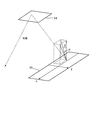
- the optical system 10 of the telescope shown in FIG. 1 has four mirrors.
- the optical system 10 of the telescope includes a first mirror 11, a second mirror 12, a third mirror 13, a plane mirror 14, and a light receiving surface 15.
- the solid line 16 represents the optical path of normal light designed to be focused on the light receiving surface 15 to form an image.
- the broken line 17 represents the optical path of the stray light that has reached the light receiving surface 15 in an irregular optical path.
- stray light analysis is to search an optical path that reaches the light receiving surface with a non-negligible light amount, following the optical path of regular light that occurs in a designed telescope.
- back propagation provides the same light path as forward propagation (forward propagation).
- forward propagation provides the same light path as forward propagation
- the third feature can not be ignored in the optical design task. Because a quantitative assessment of the probability of a fatal event occurring is often required in engineering design tasks. If the probability of occurrence of an event is very low, it can be ignored in the optical design task.
- the probabilistic sampling framework described next does not require any assumptions about the underlying fitting features, but by weighting the search space according to its fatality, it is a targeted and unknown rare
- the search is efficiently accomplished by focusing on deadly events. Furthermore, it efficiently obtains fair probability information of rare and fatal events by preserving their probability distributions throughout the search. Thus, this framework is sufficient to meet all three requirements.
- the histogram method, the multicanonical MCMC method, and the replica exchange MCMC method are representative methods of probabilistic sampling for efficiently generating events including rare and fatal events. These methods are mainly developed in the field of statistical physics, which require that events characterized by various features with their weights that preserve a given probability distribution accurately be analyzed.
- the histogram method simply samples events from events that have a distribution that is independent of their probability according to the reciprocal of their probability density function.
- the method requires a probability density function explicitly known as prior knowledge, and is supported on space with only a few dimensions for search efficiency.
- the Multicanonical MCMC method uses a single Markov Chain Monte Carlo (MCMC) method, and a single MCMC method seeks out sequential events from an implicit given probability distribution over the highest possible dimensional space. While repeating the sampling process, the Multicanonical MCMC method iteratively updates the weighting functions of the sampled events to ensure that they are uniformly distributed with respect to their fatality degree. Thus, the Multicanonical MCMC method efficiently lists various events, including targeted rare and fatal events, with their weights, which maintain their probability distribution accurately, without any bias. become.
- MCMC Markov Chain Monte Carlo
- the replica exchange MCMC method uses MCMC methods in layers in parallel, but is also known as parallel tempering or Metropolis-coupled MCMC.
- Each MCMC method follows the implicit probability distribution
- the MCMC method of the top layer follows the probability distribution of interest
- the MCMC method of the deep layer follows a flatter distribution.
- This technique exchanges, sequentially and randomly, events generated in one layer with other events in adjacent layers while meeting its detailed balance.
- the upper layer introduces events following the flatter distribution from the lower layer without disturbing its distribution, it acquires various events including rare and fatal events in the top MCMC method according to the probability distribution of interest .
- this exchange mechanism can generate rare and fatal events more efficiently than the Multicanonical MCMC method
- each step of the MCMC method is to check the fatality degree of the generated event.
- the parallel MCMC method including simulation, takes a lot of computation time.
- Multicanonical MCMC method We first describe the use of weighted sampling to find events by applying weights based on the proposed distribution. Subsequently, MCMC sampling with multi-canonical weights for efficiently sampling events including rare and fatal events will be described. Furthermore, an algorithm for obtaining an appropriate proposed distribution in the Multicanonical MCMC method is described.
- X ⁇ S is an event. It should be noted that the event space S may be discrete or continuous. When the event space S is continuous, the sum ⁇ on the subset of event space S is subsequently rewritten by ⁇ . Furthermore, the probability distribution that event X occurs is given by P (X).
- C th ⁇ [C min , C max ] is its fatality level of an event and its threshold level given to define a fatal event (hereinafter also referred to simply as “threshold”).
- threshold a threshold level given to define a fatal event
- we use a histogram consisting of the range C i , i 1,..., B on [C min , C max ].
- the height of the range C i is expressed by the following equation.
- P (C (X)) represents P (C i ).
- the fatal degree C (X) ⁇ C i .
- the fatal degree is also called an evaluation function or an energy function.
- the range C i is also called a class, and the height (number of events) of the range C i is also called a frequency.
- c is a constant
- Eq. 5 is obtained on ⁇ X ⁇ S
- C (X) ⁇ C i ⁇ for all value ranges C i , i 1,. .
- a Z ⁇ S P (X) / P (C (X)).
- the MCMC method is used to efficiently sample the event X from the proposed distribution Q (X), since the event X is generally a high-dimensional vector.
- the simplest algorithm is the entropic sampling method, in which all multi-canonical weights G (C i ) are updated after a sufficiently large number of sampled events have been accumulated in the range.
- the One Landau method updates the range directly after sample events are generated in the range by the MCMC method. This frequent update more efficiently estimates the objective multicanonical weight G (C (X)).
- I (C th ⁇ C (X i )) is an indicator function and is defined as the following equation 7.
- Equation 9 is used.
- event X by a vector that provides the operating conditions of the target system. It is assumed that the event X follows a given probability distribution P (X).
- the MCMC method is used to generate an event X that follows the proposed distribution Q (X) initially identical to the probability distribution P (X) under multi-canonical weights G (C i ).
- i 1,..., B, and all histograms are uniform (all bins are uniform).
- the simulation of the target system Sim (X) is derived using the event X generated as the input operating condition, and the fatal degree in the situation of the simulation result from the input event X is given to the heuristic It is evaluated by the measure (evaluation function) C (X).
- This fatality level updates the count in the range of the corresponding histogram Q (C i ) from the value of its initial zero, and the multi-canonical weight G (C i ) of the range by the one-Landau method between them Used to update.
- These updates provide updates of the proposed distribution as Q (X) ⁇ G (C (X)) P (X), and the generation and fatality of the next event X according to the new proposed distribution Q (X) by MCMC method
- a data set D consisting of M events with weights is generated, and the probability of fatal events P (R) is estimated from the data set D.
- the present invention relates to an optical system simulator Sim (X), which is commercially available and standard in the field of optical system design, including telescopes, as described below.
- This simulator shows the condition that event X is emitted from the light receiving surface 15 (see FIG. 1) of the imaging sensor by the method of back propagation (back propagation).
- ⁇ and ⁇ are, respectively, the latitudinal and longitudinal angles of the emitted light in orthogonal space.
- the normal vector of the light receiving surface 15 is 0 degrees.
- the range of angles is ⁇ [ ⁇ 90, 90] and ⁇ [ ⁇ 90, 90], respectively.
- the event (four variables) X is also called a parameter (input parameter).
- the probability distribution P (X) is given by the product of four independent Gaussian distributions as the following number 10.
- ⁇ x and ⁇ y are set as x range and y range , respectively, and ⁇ ⁇ and ⁇ ⁇ are each 90 degrees.
- the critical degree (evaluation function) C (X) is a heuristic but needs to be specified carefully. Because it defines a fatal event. In the analysis of the embodiment of the present invention, the fatal degree is due to the fact that the light beam emitted from the light receiving surface 15 under the condition X reaches the outside of the telescope through back propagation (back propagation). Mainly prescribed. cr (X) is 1 if this happens and 0 otherwise. However, cr (X) is not critical for a given condition X due to random reflections and refractions on the light path. Therefore, the intrinsic fatality degree of condition X is evaluated by obtaining the average of cr (X) for n tests such as the following equation 12.
- cr i (X) is the result in the i-th test.
- the fatal degree (evaluation function) C (X) monotonously increases with respect to the probabilistic approximation to the fatal situation, and the fatal degree (evaluation function) C (X) equal to or higher than the threshold level C th Condition X has a fatal event.
- the threshold level C th is set to 0.6, and most of the conditions X in n tests result in a fatal situation in this simulation.
- the value of n needs to be determined in consideration of the relationship between the computational cost of the critical degree (evaluation function) C (X) and the statistical stability.
- the fatal degree (evaluation function) C (X) follows the binomial distribution, and its relative standard error is approximately ⁇ (1-C (X)) / nC (X), which is It monotonously increases with n and the fatal degree (evaluation function) C (X).
- n is set to 100 in our experiments. The reason is that the error is sufficiently suppressed with respect to the fatal condition X in which the fatal degree (evaluation function) C (X) is close to one.
- the hyperparameter ⁇ governs the deviation of the new condition X ′ from the condition X. If the hyperparameter ⁇ is too large, the range in which the new condition X ′ deviates from the condition X misses the fatal event in which the new condition X ′ approaches the condition X. If the hyperparameter ⁇ is too small, then the new condition X 'remains mostly close to the condition X and hardly any fatal events away from the condition X can be found. Therefore, it is necessary to properly adjust the value of hyperparameter ⁇ using a trial and error approach method.
- the maximum number of histogram updates K max and the maximum number of MCMC steps M max were set to 10 and 5000, respectively, throughout all our experiments.
- the former is sufficient to bring F close to unity, and finely adjust the multicanonical weight G (C i ).
- the latter also allows sufficient relaxation of the MCMC process.
- th th The normalized energy of the configuration has become smaller than the threshold th th .
- This threshold th th is considered to be a non-negligible lower limit of relative light intensity. In practice, th th is set to 10 -4 times the original ray energy.
- the modes of reflection and refraction at the object are selected according to the parameters given to the object and its surface.
- angles of reflection and refraction at the object are selected stochastically according to the given parameters.
- Some rays do not split at any reflection point or any refraction point, and the incident light is attenuated to become reflected light.
- the main program including the above Algorithm 1 was implemented by Python as a programming language.
- the Light Tools Simulator was performed by the main program through the Excel VBA and Light Tools user interface for each step of the MCMC method. All calculations in our experiments were performed using a general purpose personal computer with a 3.4 GHz Intel Core i7 core processor and 16 MB of memory without additional hardware.
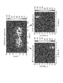
- FIG. 4 shows the result of the search for stray light in the four-dimensional parameter space.
- FIG. 4A shows a result histogram of the light ray 17 passing through an irregular path and the reaching position (x, y) on the light receiving surface 15. Higher ray counts are represented by lighter colors. This histogram shows two significant peaks that represent non-negligible non-normal rays, ie, sets of stray light.
- FIGS. 4 (b-1) and (b-2) respectively show histograms of rays belonging to the selected area around the two peaks. These are represented in the space of the incident direction ( ⁇ , ⁇ ), and clearly indicate that there are two light paths symmetrical with respect to ⁇ , which are each path that produced one of the two peaks. The results obtained for these positions and paths and the intensity of the stray light 17 correspond well to the stray light obtained in the experimental results of the full scale telescope.
- FIG. 5 (a) is a histogram showing sampled events on the critical degree (evaluation function) C (X) in the Multicanonical MCMC method of this analysis.
- the horizontal axis represents the evaluation function C (X)
- the vertical axis represents the sampled event.
- the total number of simulation tests and their calculation time to achieve this convergence and obtain the results shown in FIG. 4 were 5 ⁇ 10 4 and 17.3 hours, respectively.
- FIG. 5A shows a histogram in which the evaluation value is a class and the number of sampled events (parameters) in each class is a frequency.
- the histogram in FIG. 5A is normalized so that the maximum value of the class is 1.0.
- each event set is a meta-event for simplicity.
- Each fatal meta-event Ri is assumed to be well localized at a particular location and well separated from other fatal meta-events.
- Y) is the transition probability of event X from meta-event Y to another meta-event Y ′ in the MCMC process that generates events according to the proposed distribution Q (X). From the above assumption it is further assumed that discrete transitions between any fatal meta-events are ignored. Therefore, only non-zero transition probabilities between all R i and / R are considered. The next condition holds by the detailed balance between the state of the overall meta-event probability and R i and / R.
- c (C (X)) is represented by the following equation 24.
- Equation 6 Substituting Equations 3, 23 and 24 into Equation 6, the following Equation 26 is obtained.
- FIG. 7 shows a comparison of the number of rays obtained that cause stray light on the histogram update between the standard Multicanonical MCMC method (sm-MCMC) and the proposed Focused Multicanonical MCMC method (fm-MCMC).
- sm-MCMC standard Multicanonical MCMC method
- fm-MCMC proposed Focused Multicanonical MCMC method
- Table 2 shows the performance comparison of grid search, Bayesian optimization, standard Multicanonical MCMC method, and Focused Multicanonical MCMC method.
- Grid search is an exhaustive search algorithm of the entire event space, providing baseline performance. We have not evaluated genetic algorithms and simulated annealing. Because they are infeasible by requiring a huge number of simulations.
- the first and second columns of Table 2 indicate the probability of finding rare and fatal events for each simulation test, that is, the efficiency of the search.
- the first column shows the efficiency when searching for the direction [ ⁇ , ⁇ ] of the incident light causing the stray light by fixing the position [x, y] at the position where the stray light was observed.
- the efficiency of Bayesian optimization is one order of magnitude greater than that of grid search, while the efficiency of standard Multicanonical MCMC and Focused Multicanonical MCMC is two orders of magnitude higher.
- the second column of Table 2 shows the efficiency when searching the entire four-dimensional space. Due to the large search space, Bayesian optimization, in dealing with 10 5 number of tests, could not find any fatal events.
- the two Multicanonical MCMC methods can successfully find one rare and fatal event within 1000 trials, and this efficiency is five orders of magnitude higher than grid search.
- the efficiency of the Focused Multicanonical MCMC method is twice that of the standard Multicanonical MCMC method.
- the last column of Table 2 shows an estimate of the probability P (R) of rare and fatal events, ie the risk of stray light.
- Grid search estimates are expected to contain high uncertainty. Because grid search can only find a very limited number of rays that cause stray light, thus leading to large statistical errors. Bayesian optimization can not provide this probability. Because it does not possess probabilistic information in the search.
- the numbers 8 and 26 of the standard Multicanonical MCMC method and the Focused Multicanonical MCMC method provide estimates with the same order of magnitude as the probability obtained by the grid search.
- FIG. 8 is a block diagram showing an optical system design support system 100 according to the first embodiment of the present invention, which uses the above-mentioned optical system simulator Sim (X).
- the optical system design support system 100 is a system for discovering the possibility of generation of stray light in a designed optical system 10 such as a telescope as shown in FIG.
- the optical system design support system 100 includes a processing unit 200 and a storage unit 300.
- the processing unit 200 includes, for example, a processor such as a central processing unit (CPU), but is of course not limited to this.
- the storage unit 300 includes, for example, a random access memory (RAM) or a read only memory (ROM), but is of course not limited thereto.
- the processing unit 200 includes a parameter determination unit 210, a trajectory calculation unit 220, and an evaluation value calculation unit 230.
- the storage unit 300 includes a parameter storage unit 310, an optical model storage unit 320, and an evaluation value storage unit 330.
- the parameter determination unit 210 determines parameters as described later. As described above, the parameter determination unit 210 determines, as each parameter, a two-dimensional position (x, y) on the light receiving surface 15 of the designed optical system 10 and an angle ( ⁇ in two directions at which light enters the light receiving surface 15). , ⁇ ) to determine a combination of four dimensional variables in total.
- the parameter storage unit 310 stores the determined parameter.
- the locus calculation unit 220 uses the determined parameters to calculate the locus of the light beam in the designed optical system 10 as described later.
- the locus calculation unit 220 calculates a locus along which the light beam propagates backward from the light receiving surface 15 toward the light entrance.
- the optical model storage unit 320 stores an optical model in which a plurality of optical components are arranged on the optical path from the light entrance to the light receiving surface 15 in the designed optical system 10. This optical model corresponds to the designed optical system 10.
- the locus calculation unit 220 receives an input of the optical model stored in the optical model storage unit 320, and calculates a locus indicating the behavior of a light beam in the optical model.
- the evaluation value calculation unit 230 calculates an evaluation value indicating the possibility of generation of stray light with respect to the parameter based on comparison between the calculated locus and the locus expected under the parameter in the ideal optical system. Do. In other words, the evaluation value calculation unit 230 has an evaluation function C (X) uniquely defined according to the designed optical system 10 (optical model). That is, the optical system simulator Sim (X) has an evaluation function C (X). The evaluation value calculation unit 230 receives the calculated trajectory and the determined parameters, and calculates an evaluation value according to the evaluation function C (X). The evaluation value storage unit 330 stores the calculated evaluation value.
- the parameter storage unit 310 stores the parameters used to calculate the past trajectory.
- the evaluation value storage unit 330 stores the evaluation value calculated for the parameter.
- the parameter determination unit 210 uses for calculating the locus from the next time onward so that the higher the evaluation value, the closer to the parameter Determine the parameters.
- the parameter determination unit 210 defines a distribution of random numbers such that random numbers closer to the parameters can be obtained as the evaluation value is higher, and generates parameters to be used for calculating the next and subsequent trajectories based on this distribution.
- FIG. 9 is a block diagram showing the configuration of the parameter determination unit 210 used in FIG. 8 in detail.
- the parameter determination unit 210 includes a histogram calculation unit 212, a random number distribution definition unit 214, and a parameter generation unit 216.
- optical system design support system 100 The operation of the optical system design support system 100 will be described in more detail below with reference to FIGS. 8 and 9.
- the parameter storage unit 310 stores N parameters used to calculate a past trajectory.
- the parameter determination unit 210 determines N parameters to be used for calculating the trajectory N times from the next time on the basis of the distribution.
- the trajectory calculation unit 220 calculates N trajectories for each of the determined N parameters.
- the evaluation value calculator 230 calculates N evaluation values for each of the determined N parameters and the calculated N trajectories.
- the evaluation value storage unit 330 stores N evaluation values calculated for N parameters.
- the histogram calculation unit 212 receives N parameters used for calculation of the past trajectory from the parameter storage unit 310, and receives N evaluation values calculated for the N parameters from the evaluation value storage unit 330.
- the histogram calculation unit 212 calculates a histogram in which the evaluation value is a class and the number of parameters of each class is a frequency.
- the random number distribution definition unit 214 Based on the calculated histogram, the random number distribution definition unit 214 generates a distribution of random numbers for generating N parameters to be used for calculating N times of trajectories from the next time on, the random numbers such that the histogram becomes substantially flat. Define as obtained (see the figure on the left of FIG. 6).
- the parameter generation unit 216 generates each parameter to be used for calculation of each trajectory after the next time according to the defined distribution of random numbers. That is, as shown in FIG. 5A, the parameter generation unit 216 generates N parameters so that the histogram is substantially flat.
- the parameter determination unit 210 determines N parameters to be used for calculating N times of trajectories from next time using the standard Multicanonical MCMC method.
- the optical system design support system 100 may determine N parameters so that the histogram is finally substantially flat as shown in FIG. 5A by repeating the above operation a plurality of times. it can.
- substantially flat means that the frequency in each class falls within a predetermined error range with respect to the average frequency. This will be described by taking the case of FIG. 5 (a) as an example. It is assumed that the average frequency is 75 and the predetermined error is 15. In this case, the frequency in each class is in the range of 60 to 90.
- FIG. 10 is a block diagram showing an optical system design support system 100A according to a second embodiment of the present invention, which uses the above optical system simulator Sim (X).
- the optical system design support system 100A is also a system for discovering the possibility of generation of stray light in a designed optical system 10 such as a telescope as shown in FIG.
- the illustrated optical system design support system 100A has the same configuration as the optical system design support system 100 shown in FIG. 8 except that the configuration and operation of the processing unit are different as described later. Therefore, the processing unit is given the reference numeral 200A.
- the same reference numerals are assigned to components having the same functions as those shown in FIG. 8 and the description thereof will be omitted to simplify the description.
- the processing unit 200A has the same configuration as the processing unit 200 shown in FIG. 8 except that the configuration and the operation of the parameter determination unit are different as described later. Therefore, the parameter determination unit is given the reference numeral 210A.
- FIG. 11 is a block diagram showing in detail the configuration of the parameter determination unit 210A used in the optical system design support system 100A of FIG.
- the parameter determination unit 210A has the same configuration as the parameter determination unit 210 shown in FIG. 9 except that the configuration and operation of the random number distribution definition unit are different as described later. Therefore, the random number distribution definition unit is given the reference numeral 214A.
- the random number distribution definition unit 214A determines, based on the calculated histogram, the distribution of random numbers for generating N parameters to be used for calculating N times of trajectories from the next time, according to the threshold C th defined for the class of the histogram. It defines so that the random number which gives the histogram that the frequency of the parameter in each above class is higher than the frequency of the parameter in each class below threshold value Cth is obtained.
- the maximum value of the class of the histogram is normalized to be 1.0, and the threshold C th is equal to 0.6.
- Random distribution defining unit 214A is a random number that the total of the frequencies of the sum and the threshold value C th following parameters of the frequency threshold C th or more parameters determined for the class of the histogram and gives histogram as substantially equal Define the distribution so that Here, “substantially equal”, within a predetermined error range, it means that the threshold value C th or more in total with a threshold value C th following parameters of the frequency parameter frequency total and are equal.
- the parameter generation unit 216 generates, according to the defined distribution of random numbers, each parameter to be used for calculation of each locus after the next time, as shown in FIG. 5B. That is, as shown in FIG. 5B, the parameter generation unit 216 makes the histogram substantially equal to the sum of the frequencies of the parameters of the threshold C th or more and the sum of the frequencies of the parameters of the threshold C th or less. As such, N parameters are generated.
- the parameter determination unit 210A determines N parameters to be used for calculating the trajectory N times from the next time using the Focused Multicanonical MCMC method.
- the parameter determination unit 210A, the histogram, the sum of the frequencies of the sum and the threshold value C th following parameters of the frequency threshold C th or more parameters are substantially Determine N parameters to be equal.
- the optical system design support system 100A repeats the above operation a plurality of times to obtain the sum of the frequencies of parameters whose threshold is greater than or equal to the threshold C th and the frequencies of parameters whose threshold is less than the threshold C th as illustrated in FIG. N parameters can be generated such that the sum is substantially equal.
- the random number distribution definition unit 214A sets the threshold value C th to 0.6, but the random number distribution definition unit 214A may set the threshold value C th to a value larger than 0.5. However, it is preferable that the random number distribution definition unit 214A set the threshold C th within the range of 0.6 or more and 0.8 or less. However, more preferably, the random number distribution definition unit 214A sets the threshold C th to a value of 0.6. The reason is as follows.
- the number of stray lights is not limited to only one, and in most cases, there are a plurality of stray lights due to the above-described symmetry or the like.
- the threshold C th is set higher than 0.8, most of the random numbers (parameters) of evaluation values smaller than the threshold C th are discarded, and it is possible to search for other stray light It is because sex (probability) becomes very low.
- the threshold value C th is set lower than 0.6, a plurality of stray lights can not be searched efficiently. Therefore, it is preferable to set the threshold value C th to a value of 0.6.
- a plurality of stray lights in the optical system can be analyzed automatically and efficiently.
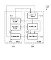
- FIG. 12 is a block diagram showing a rare event analyzer 100B according to a third embodiment of the present invention.
- the rare event analysis device 100B is a device that discovers the possibility of occurrence of a rare event. Specifically, the rare event analysis device 100B discovers, for example, stray light generated in a designed optical system 10 such as a telescope as shown in FIG. 1 as a rare event. However, the rare event analysis device 100B can be applied not only to the simulation of such a designed optical system 10 but also to the simulation of other target systems.
- the rare event analysis device 100B includes a processing unit 200B and a storage unit 300B.
- the processing unit 200 ⁇ / b> B includes, for example, a processor such as a CPU (Central Processing Unit), but of course is not limited to this.
- the storage unit 300B includes, for example, a random access memory (RAM) and a read only memory (ROM), but is of course not limited to these.
- the processing unit 200B includes a parameter determination unit 210B, a simulator 220B, and an evaluation value acquisition unit 230B.
- the storage unit 300 includes a parameter storage unit 310B and an evaluation value storage unit 330B.
- the simulator 220B may be, for example, the optical system simulator Sim (X).
- the simulator 220B can be realized by a combination of the optical model storage unit 320, the trajectory calculation unit 220, and the evaluation value calculation unit 230 shown in FIG.
- the simulator 220B is not limited to the optical system simulator Sim (X), and may be another simulator.
- the simulator 220B has an evaluation function C (X) that defines the possibility of occurrence of a rare event.
- the parameter determination unit 210B determines N parameters X k used for N simulations in each test k (1 ⁇ k ⁇ K) based on the proposed distribution Q (X). Each of the N parameters X k defines an event.
- the parameter determination unit 210B supplies the N parameters X k one by one to the simulator 220B.
- the parameter storage unit 310B stores the determined parameter.
- the evaluation value acquisition unit 230B acquires N evaluation values C (X k ) output from the simulator 220B in correspondence with the N parameters X k .
- the evaluation value storage unit 330B stores the N evaluation values.
- the parameter storage unit 310B stores N past parameters X k-1 used for N simulations of the past test (k-1).
- the evaluation value storage unit 330B stores N past evaluation values C (X k-1 ) obtained by N simulations for the N past parameters X k-1 .
- the parameter determination unit 210B compares the N past parameters X k-1 stored in the parameter storage unit 310B and the N past evaluation values C (X k-1 stored in the evaluation value storage unit 330B. And N parameters X k to be used for N simulations in the current test k, as described later.
- FIG. 13 is a block diagram showing in detail the configuration of parameter determination unit 210B used in FIG.
- the parameter determination unit 210B includes a histogram calculation unit 212B, a random number distribution definition unit 214B, and a parameter generation unit 216B.
- the histogram calculation unit 212B calculates N past parameters X k-1 stored in the parameter storage unit 310B and N past evaluation values C (X k-1 ) stored in the evaluation value storage unit 330B. Receive The histogram calculation unit 212B calculates a histogram in which the evaluation value is a class and the number of parameters of each class is a frequency.
- the random number distribution definition unit 214B determines the distribution of random numbers for generating N parameters X k used for N simulations of the current test k with respect to the class of the histogram. It is defined that a random number giving a histogram in which the frequency of the parameter in each class equal to or higher than the threshold C th is greater than the frequency of the parameter in each class lower than the threshold C th is obtained.
- the maximum value of the class of the histogram is normalized to be 1.0, and the threshold C th is equal to 0.6.
- Random distribution definition unit 214B generates a random number that the sum of the frequencies of the sum and the threshold value C th following parameters of the frequency threshold C th or more parameters determined for the class of the histogram and gives histogram as substantially equal Define the distribution so that Here, “substantially equal”, within a predetermined error range, it means that the threshold value C th or more in total with a threshold value C th following parameters of the frequency parameter frequency total and are equal.
- the parameter generation unit 216B generates each parameter X k used for each simulation in the current test k, as shown in FIG. 5 (b), based on the defined distribution of random numbers. That is, as shown in FIG. 5B, the parameter generation unit 216B makes the histogram substantially equal to the sum of the frequencies of the parameters of the threshold C th or more and the sum of the frequencies of the parameters of the threshold C th or less. Thus, N parameters X k to be used for N simulations in the current test k are generated.
- the parameter determination unit 210B determines N parameters X k to be used for N simulations in the current test k using the Focused Multicanonical MCMC method.
- the parameter determination unit 210B substantially determines that the sum of the frequencies of the parameters of the threshold C th or more and the sum of the frequencies of the parameters of the threshold C th or less To be equal, generate N parameters X k used for N simulations in the current test k.
- Rare event analysis apparatus 100B by repeating K times the test operation, as shown in FIG. 5 (b), histogram of the frequency threshold C th or more parameters sum threshold value C th following the frequency parameters N final parameters X K can be generated in the final round of testing K so that the sum is substantially equal.
- the random number distribution definition unit 214B sets the threshold value C th to 0.6, but the random number distribution definition unit 214 B may set the threshold value C th to a value larger than 0.5. However, it is preferable that the random number distribution definition unit 214B set the threshold C th within the range of 0.6 or more and 0.8 or less. However, more preferably, the random number distribution definition unit 214B sets the threshold value C th to a value of 0.6. The reason is as follows.
- the rare event is not limited to only one, and in many cases there are a plurality of rare events.
- the threshold C th is set higher than 0.8, most of the random numbers (parameters) of evaluation values (classes) smaller than the threshold C th are discarded, and other rare events
- the probability (probability) of being able to search for is extremely low.
- setting the threshold C th lower than 0.6 makes it impossible to efficiently search for a plurality of rare events. Therefore, it is preferable to set the threshold value C th to a value of 0.6.
- a plurality of rare events in the target system can be analyzed automatically and efficiently.
- Each part of the optical system design support system may be realized using a combination of hardware and software.
- an optical system design support (rare event analysis) program is developed in a RAM (random access memory), and based on the optical system design support (rare event analysis) program Each part is realized as various means by operating processor hardware such as processing unit).
- the optical system design support (rare event analysis) program may be recorded on a recording medium and distributed.
- the optical system design support (rare event analysis) program recorded in the recording medium is read into a memory via a wired, wireless, or recording medium itself to operate a processor (CPU) or the like.
- the recording medium include an optical disk, a magnetic disk, a semiconductor memory device, a hard disk and the like.
- the computer that operates as the optical system design support system is based on the optical system design support program developed in the RAM, the parameter determination unit 210, 210A, the locus This can be realized by operating as a combination of the calculation unit 220 and the evaluation value calculation unit 230.
- the computer that operates as the rare event analysis device is based on the rare event analysis program developed in the RAM, the parameter determination unit 210B, the simulator 220B, and the evaluation value acquisition unit It is possible to realize by operating as a combination of 230B.
- the present invention can be used in combination with an optical system simulator such as optical communication and a camera.
- the invention can also be used in conjunction with other simulators, such as ultimate condition search in engineering design.
- Designed optical system (telescope) 11 first mirror 12 second mirror 13 third mirror 14 plane mirror 15 light receiving surface 16 optical path of regular light 17 optical path of stray light 100, 100A optical system design support system 100B rare event analyzer 200, 200A, 200B processor 210 210A parameter determination unit 212, 212B histogram calculation unit 214, 214A, 214B random number distribution definition unit 216, 216B parameter generation unit 220 trajectory calculation unit 220B simulator 230 evaluation value calculation unit 230B evaluation value acquisition unit 300, 300B storage unit 310, 310B Parameter storage unit 320 Optical model storage unit 330, 330B Evaluation value storage unit
Landscapes
- Engineering & Computer Science (AREA)
- Physics & Mathematics (AREA)
- Theoretical Computer Science (AREA)
- Computer Hardware Design (AREA)
- Evolutionary Computation (AREA)
- Geometry (AREA)
- General Engineering & Computer Science (AREA)
- General Physics & Mathematics (AREA)
- Complex Calculations (AREA)
Abstract
目的系における極めて稀で致命的な事象を、自動的に確実に解析できる新規な方法を提供する。ヒストグラム算出部は、N個の過去のパラメータとN個の過去の評価値とを入力して、評価値を階級とし、各階級のパラメータの個数を度数とするヒストグラムを算出する。乱数分布定義部は、算出したヒストグラムに基づいて、今回の試験におけるN回のシミュレーションに使用するN個のパラメータを生成するための乱数の分布を、ヒストグラムの階級に対して定められた閾値以上の各階級でのパラメータの度数が、閾値以下の各階級でのパラメータの度数よりも多くなるようなヒストグラムを与える乱数が得られるように、定義する。パラメータ生成部は、定義した乱数の分布に基づいて、今回の試験における各シミュレーションに使用する各パラメータを生成する。
Description
本発明は、希少事象解析装置、希少事象解析方法および希少事象解析プログラム記録媒体に関する。
望遠鏡などの光学系を設計する際には、迷光が発生しないように設計する必要がある。ここで、「迷光」とは、光学設計において潜在的に起こるものであって、設計光路に従わない希少な非干渉性光線に起因して起こる光である。すなわち、非正規の経路(光路)で受光面に入ってくる光線は迷光と呼ばれ、像のコントラスト低下やノイズの原因となる。
しかしながら、非干渉性光線が複雑で大きな系において起こる条件は、非常に複雑であって、たとえ専門家が広範囲にわたる経験と優秀な直観とを持っていたとしても、迷光は稀に起こるものなので、専門家はときたまそれらを見落としてしまう。この事実は、設計されたシステムの性能低下をもたらすだけでなく、信用性と信頼性とを減少させてしまう。
一方、光学シミュレーションによって全ての可能な条件を適用して、非常に希少な条件を全て自動的に探索することは、実際問題として困難である。
迷光を解析するためのシミュレーション手法が知られている。例えば、特許文献1は、1本の光線を透過光線と反射光線とに分割し、その両方の光線を追跡することにより迷光を扱えるようにして、より正確な光線追跡法による「光学シミュレーション装置」を実現している。
しかしながら、特許文献1は、迷光という稀な事象を効率よく発見するために、光学シミュレーション装置への入力となるパラメータ(事象)の組み合わせを決定する工夫については何ら示唆も開示もしていない。
本発明の目的は、上述した課題を解決する、希少事象解析装置、希少事象解析方法および希少事象解析プログラム記録媒体を提供することにある。
本発明による希少事象解析装置は、希少事象が発生する可能性を発見する希少事象解析装置であって、提案分布Q(X)に基づいて、毎回の試験k(1≦k≦K)におけるN回のシミュレーションに使用する、各々が事象を規定するN個のパラメータXkを決定して、前記N個のパラメータXkを1つずつ順次、前記希少事象が発生する可能性を規定する評価関数C(X)を持つシミュレータに供給するパラメータ決定部と;前記N個のパラメータXkに対応して、該シミュレータから出力されるN個の評価値C(Xk)を取得する評価値取得部と;を備え、前記パラメータ決定部は、過去の試験(k-1)のN回のシミュレーションに使用したN個の過去のパラメータXk-1と、該N個の過去のパラメータXk-1に対するN回のシミュレーションで取得されたN個の過去の評価値C(Xk-1)とに基づいて、今回の試験kにおけるN回のシミュレーションに使用するN個のパラメータXkを決定し、前記パラメータ決定部は、前記N個の過去のパラメータXk-1と前記N個の過去の評価値C(Xk-1)とを入力して、評価値を階級とし、各階級のパラメータの個数を度数とするヒストグラムを算出するヒストグラム算出部と;該算出したヒストグラムに基づいて、前記今回の試験kにおけるN回のシミュレーションに使用するN個のパラメータXkを生成するための乱数の分布を、前記ヒストグラムの階級に対して定められた閾値Cth以上の各階級でのパラメータの度数が、前記閾値Cth以下の各階級でのパラメータの度数よりも多くなるようなヒストグラムを与える乱数が得られるように、定義する乱数分布定義部と;該定義した乱数の分布に基づいて、前記今回の試験kにおける各シミュレーションに使用する各パラメータXkを生成するパラメータ生成部と;を有する。
本発明の希少事象解析方法は、希少事象が発生する可能性を発見する希少事象解析方法であって、提案分布Q(X)に基づいて、毎回の試験k(1≦k≦K)におけるN回のシミュレーションに使用する、各々が事象を規定するN個のパラメータXkを決定して、前記N個のパラメータXkを1つずつ順次、前記希少事象が発生する可能性を規定する評価関数C(X)を持つシミュレータに供給する、パラメータを決定することと;前記N個のパラメータXkに対応して、該シミュレータから出力されるN個の評価値C(Xk)を取得することと;を含み、前記パラメータを決定することは、過去の試験(k-1)のN回のシミュレーションに使用したN個の過去のパラメータXk-1と、該N個の過去のパラメータXk-1に対するN回のシミュレーションで取得されたN個の過去の評価値C(Xk-1)とに基づいて、今回の試験kにおけるN回のシミュレーションに使用するN個のパラメータXkを決定することであり、前記パラメータを決定することは、前記N個の過去のパラメータXk-1と前記N個の過去の評価値C(Xk-1)とを入力して、評価値を階級とし、各階級のパラメータの個数を度数とするヒストグラムを算出することと;該算出したヒストグラムに基づいて、前記今回の試験kにおけるN回のシミュレーションに使用するN個のパラメータXkを生成するための乱数の分布を、前記ヒストグラムの階級に対して定められた閾値Cth以上の各階級でのパラメータの度数が、前記閾値Cth以下の各階級でのパラメータの度数よりも多くなるようなヒストグラムを与える乱数が得られるように、定義することと;該定義した乱数の分布に基づいて、前記今回の試験kにおける各シミュレーションに使用する各パラメータXkを生成することと:を含む。
本発明の希少事象解析プログラム記録媒体は、コンピュータに、希少事象が発生する可能性を発見する希少事象解析プログラムを記録した記録媒体であって、前記希少事象解析プログラムは、前記コンピュータに、提案分布Q(X)に基づいて、毎回の試験k(1≦k≦K)におけるN回のシミュレーションに使用する、各々が事象を規定するN個のパラメータXkを決定して、前記N個のパラメータXkを1つずつ順次、前記希少事象が発生する可能性を規定する評価関数C(X)を持つシミュレータに供給するパラメータ決定手順と;前記N個のパラメータXkに対応して、該シミュレータから出力されるN個の評価値C(Xk)を取得する評価値取得手順と;を実行させ、前記パラメータ決定手順は、前記コンピュータに、過去の試験(k-1)のN回のシミュレーションに使用したN個の過去のパラメータXk-1と、該N個の過去のパラメータXk-1に対するN回のシミュレーションで取得されたN個の過去の評価値C(Xk-1)とに基づいて、今回の試験kにおけるN回のシミュレーションに使用するN個のパラメータXkを決定させるものであり、前記パラメータ決定手順は、前記コンピュータに、前記N個の過去のパラメータXk-1と前記N個の過去の評価値C(Xk-1)とを入力して、評価値を階級とし、各階級のパラメータの個数を度数とするヒストグラムを算出するヒストグラム算出手順と;該算出したヒストグラムに基づいて、前記今回の試験kにおけるN回のシミュレーションに使用するN個のパラメータXkを生成するための乱数の分布を、前記ヒストグラムの階級に対して定められた閾値Cth以上の各階級でのパラメータの度数が、前記閾値Cth以下の各階級でのパラメータの度数よりも多くなるようなヒストグラムを与える乱数が得られるように、定義する乱数分布定義手順と;該定義した乱数の分布に基づいて、前記今回の試験kにおける各シミュレーションに使用する各パラメータXkを生成するパラメータ生成手順と;を実行させる。
本発明によれば、目的系における極めて稀で致命的な事象を、自動的に確実に解析できる。
まず、本発明の理解を容易にするために、本明細書中で使用する用語の意味に関して簡略的に説明する。
マルコフ連鎖モンテカルロ法(MCMC法:Markov chain Monte Carlo methods)とは、求める確率分布を均衡分布として持つマルコフ連鎖を作成することをもとに、確率分布のサンプリングを行うアルゴリズムの総称である。換言すれば、MCMC法は、その名の示す通り「マルコフ連鎖」と「モンテカルロ法」とを組み合わせた方法である。具体的には、MCMC法は、マルコフ連鎖(Markov chain)と呼ばれる確率過程の性質を利用して確率分布からサンプリングを行い、様々な計算を行う方法である。
マルチカノニカル法(Multicanonical algorithm)とは、MCMC法におけるサンプリング法の一つで、メトロポリス・ヘイスティング法により任意の形を持つ被積分関数を積分するときに用いられる。マルチカノニカル法では、サンプリングを状態密度の逆数に従って行う。マルチカノニカル法においては、状態密度はあらかじめワン・ランダウ法などの他の方法により計算しておく。
メトロポリス・ヘイスティング法(もしくはM-Hアルゴリズム)(Metropolis-Hastings algorithm)は、直接サンプリングするのが難しい確率分布から統計標本の配列を生成するのに用いられるマルコフ連鎖を構築するのに用いられる手法である。この配列は、MCMC法において、目標分布の近似(ヒストグラム)として用いられたり、期待値のような積分計算を必要とするものに用いられる。
ワン・ランダウ法(Wang and Landau algorithm)とは、系の状態密度を計算するために用いられるモンテカルロ法のひとつである。ワン・ランダウ法では状態密度の計算に必要な、系の取り得る全ての状態のエネルギを迅速に計算するため、非マルコフ連鎖ランダムウォークを行なう。ワン・ランダウ法は、マルチカノカル法の実行に必要となる、状態密度を計算するために重要である。
本発明の要旨の一つは、望遠鏡のような光学系の設計段階における迷光(希少事象)の発見という用途に、Multicanonical MCMC法を適用したことである。
しかしながら、両者を組み合わせることは次の理由により容易ではない。
何故なら、Multicanonical MCMC法は、長い尻尾を持つ分布に従う乱数を生成するためのいくつかの科学・数学分野においては使用されているが、工学分野における長い尻尾を一般に持たない希少事象解析には使用されていないからである。
また、Multicanonical MCMC法は、統計数学、物理、および化学における種々の分野において応用されてきた。例えば、Multicanonical MCMC法は、ランダム行列、ランダムグラフ、カオス動力学の非常に希少な実例をサンプリングするために使用された。より応用向けの側面において、Multicanonical MCMC法は、遠隔通信における誤り訂正符号の理想的な性能を理論的に評価するための希少雑音をサンプリングするために使用された。しかしながら、実用的な現実世界問題のための、Multicanonical MCMC法の適用可能性とスケーラビリティは、論証されていないからである。
一般に、迷光解析のためのシミュレーション手法では、逆伝播により設計された望遠鏡の受光面から光路(光線)のシミュレーションをスタートし、正規の入光口以外の場所に終着した光路(光線)があった場合(すなわち、正しい光路以外の光路があった場合)に、その光路(光線)を迷光の可能性があると判断する。
受光面は、水平方向および垂直方向の2次元座標の点(x、y)で表され、各点に対して光路(光線)が緯度方向および経度方向の角度α、βで表される。すなわち、一本の光路(光線)は、4つの変数(x、y、α、β)から成る一組のパラメータ値で表されることになる。換言すれば、各光路(光線)は、4つの変数(一組のパラメータ値)で規定される(4つのパラメータを座標とする4次元空間上のベクトルで規定される)。そのため、迷光を探索するには、上記4つの変数(一組のパラメータ値)を順次変えながら、膨大な数の光路(光線)に対してシミュレーションを行うことが必要となる。
[発明の概要の説明]
本発明者らは、この統計的サンプリング手法を、信用できかつ信頼できる工学設計のために、非常に希少で致命的な事象の探索に応用する。本発明の提案は次のように要約される。
本発明者らは、この統計的サンプリング手法を、信用できかつ信頼できる工学設計のために、非常に希少で致命的な事象の探索に応用する。本発明の提案は次のように要約される。
本発明者らは、Multicanonical MCMC法を使用して目的系における非常に希少で致命的な事象を自動的にかつ確実に解析する新規な手法を提案する。
本発明者らは、また、希少で致命的な事象のより効率的な探索を達成する目的のために、特に、Multicanonical MCMC法の拡張を提案する。
本発明者らは、望遠鏡の実スケールの設計を使用した実験において、本発明者らの方法の優れた能力を確認し、本発明者らの解析は、103のシミュレーション試験のオーダ内で、成功のうちに全ての迷光を発見できた。これは、公知のグリッドサーチに基づくシミュレーションによって必要な試験の数よりも、5桁も少ない大きさである。ここで、「グリッドサーチ」とは、パラメータの組み合わせを、総当たりで探して探索したい事象(本迷光解析の例では迷光)を発生させるパラメータを探索する方法をいう。
[迷光用の探索のための解析]
迷光解析の目的は、望まれない光線が撮像素子の受光面に伝搬したかどうか、その強度が画像における雑音を引き起こすのに十分に大きいかどうかを決定することである。例えば、図1に示される望遠鏡の光学系10は、4つの鏡を持つ。
迷光解析の目的は、望まれない光線が撮像素子の受光面に伝搬したかどうか、その強度が画像における雑音を引き起こすのに十分に大きいかどうかを決定することである。例えば、図1に示される望遠鏡の光学系10は、4つの鏡を持つ。
図1において、望遠鏡の光学系10は、第1の鏡11と、第2の鏡12と、第3の鏡13と、平面鏡14と、受光面15とを備える。
図1において、実線16は、画像を形成するために受光面15上に焦点を合わすように設計された正規光の光路を表す。他方、破線17は、受光面15に非正規の光路で到達した迷光の光路を表す。
迷光解析の目的は、設計された望遠鏡において起こる、正規光の光路以外をたどって無視できない光量で受光面に達する光路を探索することである。
迷光解析のためのツールは、2つのモンテカルロ原理の1つを使用することによって主に進展された。簡単な手法は、光線が与えられた光源においてあるランダムな位置からランダムな角度で出射される、前方伝播(順伝播)原理を使用することであり、望遠鏡の受光面での到達を評価する。この原理は、シミュレートされるべき出射の広い範囲の位置と角度とを必要とする。何故なら、光源は潜在的に望遠鏡を囲んでいるからである。したがって、前方伝播(順伝播)を使用する解析は、一般的には効率が悪くなる傾向がある。この困難さのために、迷光を解析するための大抵のツールは、光線が望遠鏡の受光面上のランダムな位置からランダムな角度で仮想的に出射される、後方伝播(逆伝播)原理を使用し、望遠鏡の外部へのそれらの存在をチェックする。分光計のような光の入出力特性が非対称な光学変換装置を除いて、望遠鏡の全ての光学要素は、光線の入射および出射に関して対称的である。したがって、後方伝播(逆伝播)は、前方伝播(順伝播)と同一の光路を提供する。後者の原理は、前者よりも効率的である。何故なら、光が受光面から放出される角度と位置の範囲は、ほとんどの場合において制限されるからである。
迷光の発生確率が非常に低い場合、後方伝播(逆伝播)原理を使用するツールの効率は、迷光のしらみつぶし探索を可能にするには不十分である。したがって、これらのツールは、専門家によって迷光の発生に向けて発見的に受光面に達する幾つかの光路をシミュレートするために使用される。専門家の知識とこのツールとを組み合わせた合成法を提案して、迷光解析の信頼性と効率性とを増加することを試みている。しかしながら、人間の専門家によって行われる解析は、専門家のスキルと知識とに依存し、ある場合にはすべての迷光を探索できない。何故なら、迷光の発生する条件は、非常に複雑で、稀に起こるからである。加えて、人間の解析は、熟練した専門家の制限された有用性を扱えない。
[工学設計のための希少で致命的な事象探索]
多くの工学設計のタスクにおいて与えられる、致命的な結果を引き起こす希少事象を発見するには、次の特徴が必要である。
多くの工学設計のタスクにおいて与えられる、致命的な結果を引き起こす希少事象を発見するには、次の特徴が必要である。
(1)多数の種類の希少で致命的な事象が、不連続かつ非線形と複雑性とによって特徴づけられる実世界システムにおいて効率的に探索される。
(2)暗黙に与えられかつ非常に低い発生に従う事象が、効率的に探索される。
(3)事象発生の確率が、定量的に評価される。
(2)暗黙に与えられかつ非常に低い発生に従う事象が、効率的に探索される。
(3)事象発生の確率が、定量的に評価される。
3番目の特徴を光学設計タスクでは無視することができない。何故なら、致命的な事象が発生する確率の定量的な評価は、工学設計タスクにおいてしばしば要求されるからである。事象の発生確率が非常に低い場合、光学設計タスクでは無視することがありうる。
(1)に関して、探索空間において目標関数のある特定の特徴を仮定する、凸状最適化のような方法は、この問題に適用できない。何故なら、特徴の種類が未知であるからである。この観点において、進化的最適化フレームワーク、確率的最適化フレームワーク、情報科学的最適化フレームワークが、迷光条件を探索するための候補となる。何故なら、それらは、多数の局所極大を探索できるからである。例えば、遺伝的アルゴリズムやシミュレーテッド・アニーリングが代表的なアルゴリズムであり、しばしば、種々の問題において多数の局所極大を見つけるためによく実行される。何故なら、これらのアルゴリズムは、理想的には、根本的な適合特徴についての何らの仮定も必要としないからである。近年、ベイズ最適化が、種々の工学応用においてしばしば使用されている。これは、未知で根本的な適合特徴が、ガウス過程のようないくつかの原理によって生成された代理のモデルによって良く近似されることを仮定しており、特徴推定の最も高い不確かさの点を評価することによって、特徴の局所極大を探す。この手法は、目的とする特徴関数が、評価するために費用が高く、微分不可能で、非凸で、かつ多峰性があるとき、効果的でかつ効率的である。
しかしながら、これらフレームワークの探索原理がご都合主義で、確率的であるために、それらは、その非常に低い未知の確率のために不測の出来事によって見つけられる必要がある、高く分離しかつ高く局所化された極大を容易に見落としてしまう。加えて、最適化手法は、一般的に、システムにおける希少で致命的な事象の発生の確率についての情報を提供しない。何故なら、それらはそれらの探索機構において事象発生の確率分布を評価しないからである。したがって、これらの手法は、要求(2)および(3)を満足しない。
対照的に、次に述べる確率的サンプリングフレームワークは、また根本的な適合特徴についてなんら仮定を必要とないが、その致命的な度合いに従って探索空間を重み付けることによって、目的のかつ未知の希少で致命的な事象に焦点を当てることによって、探索を効率的に達成する。更に、それは、探索の間じゅうそれらの確率分布を保存することによって希少で致命的な事象の公平な確率情報を効率的に獲得する。従って、このフレームワークは、3つの要求の全てを満たすのに十分である。
[希少で致命的な事象の効率的な確率論的なサンプリング]
ヒストグラム法、Multicanonical MCMC法、およびレプリカ交換MCMC法が、希少で致命的な事象を含む事象を効率的に生成するための確率論的なサンプリングの代表的な方法である。これらの方法は、主に、与えられた確率分布を正確に保存するそれらの重みを持つ種々の特徴によって特徴づけられた事象が解析されるのを必要とする、統計物理の分野において開発されてきた。
ヒストグラム法、Multicanonical MCMC法、およびレプリカ交換MCMC法が、希少で致命的な事象を含む事象を効率的に生成するための確率論的なサンプリングの代表的な方法である。これらの方法は、主に、与えられた確率分布を正確に保存するそれらの重みを持つ種々の特徴によって特徴づけられた事象が解析されるのを必要とする、統計物理の分野において開発されてきた。
ヒストグラム法は、簡単に、それらの確率密度関数の逆数に従って、それらの確率に独立な分布を持つ事象から、事象をサンプリングする。しかしながら、その方法は、先行知識として明示的に知られている確率密度関数を必要とし、探索効率のために少ない次元のみを持つ空間上で支持される。
Multicanonical MCMC法は、単一のマルコフ連鎖モンテカルロ(MCMC)法を使用し、単一のMCMC法は、できるかぎり高い次元空間上の黙示的に与えられた確率分布から順次事象を探し出す。サンプリング工程を繰り返している間、Multicanonical MCMC法は、サンプルされた事象の重み関数を反復して更新して、それらが致命的な度合いに関して一様に分布されるのを保証する。従って、Multicanonical MCMC法は、何らの片寄りなく、それらの確率分布を正確に維持するそれらの重みを持って、目標とする希少で致命的な事象を含む種々の事象を効率的に列挙することになる。
レプリカ交換MCMC法は、層状にMCMC法を並列に用いるが、parallel tempering又はMetropolis-coupled MCMCとしてもまた知られている。各MCMC法は、暗黙に与えられた確率分布に従い、最上層のMCMC法は、対象の確率分布に従い、深層のMCMC法は、より平坦な分布に従う。この技法は、それの詳細釣り合いを満たしている間、隣接する層において他の事象を持つ1つの層において生成された事象を、順次およびランダムに交換する。上位層が、それの分布を乱すことなく、低い層からのより平坦な分布に従う事象を導入するので、対象の確率分布に従う最上MCMC法における希少で致命的な事象を含む種々の事象を取得する。この交換メカニズムは、Multicanonical MCMC法よりも希少で致命的な事象をより効率的に発生することができるけれども、個々のMCMC法の各工程が生成された事象の致命的な度合いをチェックするためのシミュレーションを含む、並列MCMC法の為に、多大の計算時間がかかる。
ずっと、これらの技法は、統計数学、物理、および化学における種々の分野において応用されてきた。例えば、それらは、ランダム行列、ランダムグラフ、カオス動力学の非常に希少な実例をサンプリングするために使用された。より応用向けの側面において、これらの技法は、遠隔通信における誤り訂正符号の理想的な性能を理論的に評価するための希少雑音をサンプリングするために使用された。しかしながら、実用的な現実世界問題のためのこれらの技法の適用可能性とスケーラビリティは、論証されていない。
本発明者らが提案する、高い信頼性を要求する工業設計のための非常に希少で致命的な事象探索の手法は、Multicanonical MCMC法を使用し、この研究は、特に、非常に複雑で不連続な特徴を持つ、望遠鏡の迷光解析に適用する。この手法は、モンテカルロシミュレータによって生成された光学事象の確率分布が明白には知られておらず、かつシミュレータによる事象の生成が高価であるような問題に適している。
[Multicanonical MCMC法]
本発明者らは、最初に、提案分布に基づいて重みを適用することによって、事象を探し出すための重点サンプリングの使用について説明する。引き続いて、希少で致命的な事象を含む事象を効率的にサンプルためのマルチカノニカル重みを持つMCMCサンプリングを説明する。更に、Multicanonical MCMC法における適切な提案分布を得るアルゴリズムを説明する。
本発明者らは、最初に、提案分布に基づいて重みを適用することによって、事象を探し出すための重点サンプリングの使用について説明する。引き続いて、希少で致命的な事象を含む事象を効率的にサンプルためのマルチカノニカル重みを持つMCMCサンプリングを説明する。更に、Multicanonical MCMC法における適切な提案分布を得るアルゴリズムを説明する。
離散事象空間Sを与えたとき、X∈Sは事象である。事象空間Sは離散でも連続でもあってよいことに注意されたい。事象空間Sが連続であるとき、事象空間Sの部分集合上の総和Σは、以後∫によって書き直される。さらに、事象Xが起こる確率分布は、P(X)で与えられる。確率分布P(X)は、目的が人工システムである多くの工学設計問題において明示的に与えられるが、確率分布P(X)は、自然の物を伴う多くの問題において過去に観察された記録によって暗黙に与えられる。本発明者らは、致命的な事象R={X∈S|Cth≦C(X)}の集合を定義する。ここで、

およびCth∈[Cmin,Cmax]は、事象の致命的な度合いおよび致命的な事象を規定するために与えられたその閾値レベル(以下、単に「閾値」とも呼ぶ。)である。ここで、本発明者らは、[Cmin,Cmax]上での値域Ci、i=1、・・・、Bから成るヒストグラムを使用する。ここで、値域Ciの高さは、次式で表される。

事象Xが非常に低い確率で発生する確率分布P(X)を持つ致命的な事象であると仮定し、確率分布P(X)から直接探し出すことによっては、希少な事象Xをほとんど得ることができない。したがって、目的は、与えられた確率分布P(X)の下で閾値Cth≦C(X)を満足する希少で致命的な事象を効率的に導き出すことと、全体の希少で致命的な事象Rの確率:P(R)=P(Cth≦C(C))の良好な推定を得ることである。
[重点サンプリング]
与えられた確率分布P(X)に対して致命的な事象を効率的に生成するために、本発明者らは、事象がRにおいてマルチカノニカル重みG(C(X))によって人工的に引き上げられた提案分布Q(X)∝G(C(X))P(X)からサンプルされる、重点サンプリングを適用する。重点サンプリングとは、重みが付いたサンプルを用いて期待値を求める方法のことをいう。ここで、本発明者らは、確率分布P(X)≠0のときはいつでも提案分布Q(X)≠0であると仮定している。
与えられた確率分布P(X)に対して致命的な事象を効率的に生成するために、本発明者らは、事象がRにおいてマルチカノニカル重みG(C(X))によって人工的に引き上げられた提案分布Q(X)∝G(C(X))P(X)からサンプルされる、重点サンプリングを適用する。重点サンプリングとは、重みが付いたサンプルを用いて期待値を求める方法のことをいう。ここで、本発明者らは、確率分布P(X)≠0のときはいつでも提案分布Q(X)≠0であると仮定している。
[マルチカノニカル重みを持つMCMCサンプリング]
適切な提案分布Q(X)の選択は、重点サンプリングにおける希少で致命的な事象を含む事象の効率的な発生の鍵である。Multicanonical MCMC法は、近似的に次の数3および数4で表される提案分布Q(X)を選択する。
適切な提案分布Q(X)の選択は、重点サンプリングにおける希少で致命的な事象を含む事象の効率的な発生の鍵である。Multicanonical MCMC法は、近似的に次の数3および数4で表される提案分布Q(X)を選択する。


数4を数3に代入することによって、すべての値域Ci、i=1、・・・、Bに対して{X∈S|C(X)∈Ci}上で、数5が得られる。

[提案分布の反復推定]
前述したように、確率分布P(X)が与えられるが、確率分布P(X)は、多くの実際的な問題において直接には与えられず、したがって、数4は、マルチカノニカル重みG(C(X))を得るために直接的に適用されえない。したがって、本発明者らは、すべてのMCMCステップにおいて反復修正を使用してマルチカノニカル重みG(C(X))を効率的に推定するために、ワン・ランダウ法を適用する。
前述したように、確率分布P(X)が与えられるが、確率分布P(X)は、多くの実際的な問題において直接には与えられず、したがって、数4は、マルチカノニカル重みG(C(X))を得るために直接的に適用されえない。したがって、本発明者らは、すべてのMCMCステップにおいて反復修正を使用してマルチカノニカル重みG(C(X))を効率的に推定するために、ワン・ランダウ法を適用する。
鍵となるアイデアは、各値域Ci、i=1、・・・、BでG(C(X))を徐々に修正して、対応する提案分布Q(C(X))が区間[Cmin、Cmax]上で一様となることを保証することである。最も簡単なアルゴリズムは、すべてのマルチカノニカル重みG(Ci)が、十分に多数のサンプルされた事象が値域において蓄積された後に、更新される、エントロピック・サンプリング法である。対照的に、ワン・ランダウ法は、サンプル事象がMCMC法によって値域において生成された後に、直接的に値域を更新する。この頻繁な更新は、より効率的に、目的のマルチカノニカル重みG(C(X))を推定する。
ワン・ランダウ法は、次のように働く。MCMCプロセスの各ステップの後に、もし生成された事象が値域Ciに属するなら、対応するマルチカノニカル重みG(C(X))は、一定係数0<F<1によって乗算される。この更新は、ヒストグラムがほとんど平坦になるまで繰り返される。この点で、全てのヒストグラム値域が0にリセットされ、Fは√Fに修正される。それから、マルチカノニカル重みG(Ci)の上記更新は、ヒストグラムが十分に平坦になるまで、再び繰り返される。最後に、マルチカノニカル重みG(Ci)、i=1、・・・、Bを取得し、それは十分に一様な提案分布Q(C(X))を保証する。
[希少で致命的な事象の確率]
提案分布Q(X)から探し出されたサンプルXi、i=1、・・・、Mを与えると、致命的な事象の集合Rの確率が次の数6として与えられる。
提案分布Q(X)から探し出されたサンプルXi、i=1、・・・、Mを与えると、致命的な事象の集合Rの確率が次の数6として与えられる。




[希少迷光探索のための方法論]
本発明者らは、望遠鏡の工学設計のためのシミュレーションを基にした希少迷光探索の新しい方法論を提案する。この方法論は、上記Multicanonical MCMC法と目標とする望遠鏡のシミュレータとから成る。
本発明者らは、望遠鏡の工学設計のためのシミュレーションを基にした希少迷光探索の新しい方法論を提案する。この方法論は、上記Multicanonical MCMC法と目標とする望遠鏡のシミュレータとから成る。
本発明者らは、事象Xを、目標系の動作条件を提供するベクトルによって定義する。事象Xは、与えられた確率分布P(X)に従うと仮定する。MCMC法は、マルチカノニカル重みG(Ci)の下で確率分布P(X)と初期に同一な提案分布Q(X)に従う事象Xを生成するために使用される。ここで、i=1、・・・、Bで、全てのヒストグラムの階級で一様(ビン幅がすべて一様)である。それから、目的系Sim(X)のシミュレーションは、入力動作条件として生成された事象Xを使用して導かれ、入力事象Xからのシミュレーションの結果の状況における致命的な度合いは、ヒューリスティックに与えられた測度(評価関数)C(X)によって評価される。この致命的な度合いは、その初期ゼロの値から対応するヒストグラムQ(Ci)の値域におけるカウントを更新し、かつ、その間の上記ワン・ランダウ法によって値域のマルチカノニカル重みG(Ci)を更新するために使用される。これらの更新は、Q(X)∝G(C(X))P(X)として提案分布の更新を提供し、MCMC法による新しい提案分布Q(X)に従う次の事象Xの生成と致命的な度合い(評価関数)C(X)を提供する目的系のシミュレーションが繰り返される。このプロセスは、ヒストグラムQ(Ci)、i=1、・・・、Bがほとんど平坦になるまで続き、マルチカノニカル重みG(Ci)、i=1、・・・、Bが満足な程度に収束し、十分な数の事象Xが蓄積される。
次の表1のAlgorithm 1は、この方法の擬似コードを表す。それは、二重の’while’ループを含み、内側のループは、出力ヒストグラムQ(Ci)、i=1、・・・、Bが十分に一様になるまで、提案分布Q(X)に対してMCMC法を続けることを意図し、外側のループは、それが最終的に最適に達するまで、マルチカノニカル重みG(Ci)、i=1、・・・、Bの修正を繰り返すことを意図している。本発明者らは、遷移関数Tδ(X)を、標準MCMCアルゴリズムである、メトロポリス法を適用して、現在の事象Xから次の候補事象X’を生成する。マルチカノニカル重みG(Ci)の収束が最適になった後、重みを持つM事象から成るデータ集合Dが生成され、致命的な事象の確率P(R)はデータ集合Dから推定される。

以下、本発明を実施する形態について図面を参照して詳細に説明する。以下の各実施形態に記載されている構成は単なる例示であり、本発明の技術範囲はそれらには限定されない。
[発明の概略]
[発明の概略]
本発明は、光学系シミュレータSim(X)に係り、それは、後述するように、望遠鏡を含む、光学系設計の分野において商業上利用可能で、標準である。このシミュレータは、事象Xは、光線が後方伝播(逆伝播)の方法によって撮像センサの受光面15(図1参照)から放射される、条件を示している。従って、事象Xは条件とも呼ばれる。それは、図3に示されるような、4つ変数X=[x,y,α,β]Tから成る。図3において、xおよびyは、それぞれ、x∈[-xrange、xrange]、y∈[-yrange、yrange]として規定される受光面15上の出射の水平位置および垂直位置である。加えて、αおよびβは、それぞれ、直交空間における出射された光線の緯度方向および経度方向の角度である。受光面15の法線ベクトルは、0度である。角度の範囲は、それぞれ、α∈[-90、90]、β∈[-90、90]である。事象(4つの変数)Xは、パラメータ(入力パラメータ)とも呼ばれる。
確率分布P(X)は、次の数10として4つの独立ガウス分布の積によって与えられる。


この分布は、非常に広く、それは、中心でわずかに高いが、受光面の垂直方向において、ほとんど一様である。この確率分布P(X)の選択は、望遠鏡の対称幾何学と鏡構成を反映している。
致命的な度合い(評価関数)C(X)は、ヒューリスティックであるが注意深く指定される必要がある。何故なら、それは、致命的な事象を規定しているからである。本発明の実施の形態の解析において、致命的な度合いは、条件Xの下での受光面15から出射された光線が、後方伝播(逆伝播)を介して望遠鏡の外側へ到達するという事実によって主に規定される。cr(X)は、もしこれが起こったら1であり、それ以外は0である。しかしながら、cr(X)は、光路上のランダムな反射と屈折のために、与えられた条件Xに対して決定的でない。したがって、条件Xの本質的な致命的な度合いは、次の数12のようなn個の試験に対してcr(X)の平均を取得することによって評価される。

本発明者らは、出力X’が次の数13のように条件Xで中心に置かれる多変数の独立分布されたガウスによってランダムに与えられる、次の遷移関数Tδ(X)を使用する。


ヒストグラム更新の最大数KmaxとMCMC工程の最大数Mmaxを、本発明者らのすべての実験を通して、それぞれ、10および5000に設定した。前者は、Fを単位元に近づけるために十分であり、マルチカノニカル重みG(Ci)を細かく調整する。後者は、また、MCMCプロセスの十分な緩和を可能とする。調整されるべき最後のパラメータは、致命的な度合い(評価関数)C(X)上のヒストグラム値域の数Bである。最大数Mmax以下の事象は、これらB個の値域上に一様に分散されるので、1つの値域におけるすべての事象の起こる確率は同じであり、1つの値域における事象の数は、その相対的な標準偏差ε≦√(B/Mmax)を持つポアソン分布に従う。本発明者らは、B=20に設定し、それは適度に小さいε=0.05~0.10を維持する。
[実施の形態]
次に、実施の形態を用いて、本発明を実施するための形態を説明する。
次に、実施の形態を用いて、本発明を実施するための形態を説明する。
[実験セットアップ]
本発明者らは、シノプシス社(Synopsys, Inc)によって発売された、Light Toolsという名前の照明設計解析ソフトウェアを使用した。このソフトウェアは、光学設計および解析において広く利用されている。このソフトウェアはモンテカルロ光線追跡が可能である。目的の光学系は、設計された望遠鏡の本物スケールの実物大模型である。本発明者らは、経験的に、2つの光路が、望遠鏡の幾何学的対称性のために、受光面15の2つの対称領域で同様の強度の迷光を引き起こすことを知っている。
本発明者らは、シノプシス社(Synopsys, Inc)によって発売された、Light Toolsという名前の照明設計解析ソフトウェアを使用した。このソフトウェアは、光学設計および解析において広く利用されている。このソフトウェアはモンテカルロ光線追跡が可能である。目的の光学系は、設計された望遠鏡の本物スケールの実物大模型である。本発明者らは、経験的に、2つの光路が、望遠鏡の幾何学的対称性のために、受光面15の2つの対称領域で同様の強度の迷光を引き起こすことを知っている。
このシミュレーションの仮定と条件は、次の通りである。
・本発明者らは、シミュレーションにおいて使用されるモデルが、実際の世界の実物大模型の系の完全な複製であると仮定する。
・迷光を生成するためのメカニズムは、幾何学的光学のみによってよく近似される。
・すべての追跡された光線は、単一の波長によってよく近似される。
・「逆伝播法」が、すべの実験において効率的な解析のために使用される。
・光線追跡は、次の条件のどちらかで停止される。
・本発明者らは、シミュレーションにおいて使用されるモデルが、実際の世界の実物大模型の系の完全な複製であると仮定する。
・迷光を生成するためのメカニズムは、幾何学的光学のみによってよく近似される。
・すべての追跡された光線は、単一の波長によってよく近似される。
・「逆伝播法」が、すべの実験において効率的な解析のために使用される。
・光線追跡は、次の条件のどちらかで停止される。
-構成の正規化エネルギξが閾値ξthより小さくなった。この閾値ξthは、無視できない相対的光線強度の下限であるとみなされる。実際には、ξthは、元光線エネルギの10-4倍に設定される。
-光線が、何らかの障害物に遭遇することなく、望遠鏡の外側の無限空間へ到達する。
・反射と屈折は次のように計算される。
・反射と屈折は次のように計算される。
-物体での反射および屈折のモードは、その物体とその表面に与えられたパラメータに従って選択される。
-物体での反射および屈折の角度は、与えられたパラメータに従って確率的に選択される。
-ある光線は、どの反射点およびどの屈折点においても分岐せず、入射光が減衰して反射光となる。
上記Algorithm 1を含む主なプログラムを、プログラム言語であるパイソン(Python)によって実装した。MCMC法の各ステップを、Light Toolsシミュレータは、Excel VBAとLight Toolsのユーザインタフェースを介して主プログラムによって実行された。本発明者らの実験における全ての計算を、付加的なハードウェアなしで、3.4GHzのIntel Core i7コアプロセッサと16MBのメモリとを備えた汎用パーソナルコンピュータを使用した実行した。
[実験結果]
本発明者らは、上記[方法論]と上記[セットアップ]を使用して、迷光解析を実施した。図4は、4次元パラメータ空間における迷光の探索の結果を示す。
本発明者らは、上記[方法論]と上記[セットアップ]を使用して、迷光解析を実施した。図4は、4次元パラメータ空間における迷光の探索の結果を示す。
図4(a)は、非正規な経路を通過する光線17と受光面15上の到達位置(x,y)の結果ヒストグラムを示す。より高い光線カウントをより明るい色で表している。このヒストグラムは、無視できない非正規の光線、すなわち、迷光の組を表す、2つの重要なピークを示している。
図4(b-1)および(b-2)は、それぞれ、この2つのピークの周りの選択された領域に属する光線のヒストグラムを示す。これらは、入射方向(α,β)の空間において表され、明らかに、2つのピークの1つを生成した各経路である、βに関して対称な2つの光路が存在することを示している。これら位置、経路に対して得られた結果と迷光17の強度は、実物大模型の望遠鏡の実験結果で得られた迷光とよく対応する。
図5(a)は、この解析のMulticanonical MCMC法における致命的な度合い(評価関数)C(X)上のサンプルされた事象を示すヒストグラムである。図5(a)において、横軸は評価関数C(X)を示し、縦軸はサンプルされた事象を示す。この収束を達成して、図4に示される結果を得るための、シミュレーション試験の総数とそれらの計算時間は、それぞれ、5×10⁴と17.3時間であった。
図5(a)は、評価値を階級とし、各階級のサンプルされた事象(パラメータ)の個数を度数とするヒストグラムを示している。図5(a)のヒストグラムは、階級の最大値が1.0となるように正規化されている。
[希少事象探索のために特殊化されたMulticanonical MCMC法]
上述したように、この手法は、事象をサンプルするために標準Multicanonical MCMC法に従っており、与えられた確率分布を正確に維持する重みを持つ希少事象を含んでいる。これは、希少事象確率P(R)と、統計物理や他の応用分野におけるその関連する統計値とを正確に解析することが必要である。正確な重みは、統計偏差を避けるために致命的な度合いの領域[Cmin,Cmax]上で種々の事象を生成することによって取得され、したがって、目的ヒストグラムQ(Ci)、i=1、・・・、Bは、一様に設定される。
上述したように、この手法は、事象をサンプルするために標準Multicanonical MCMC法に従っており、与えられた確率分布を正確に維持する重みを持つ希少事象を含んでいる。これは、希少事象確率P(R)と、統計物理や他の応用分野におけるその関連する統計値とを正確に解析することが必要である。正確な重みは、統計偏差を避けるために致命的な度合いの領域[Cmin,Cmax]上で種々の事象を生成することによって取得され、したがって、目的ヒストグラムQ(Ci)、i=1、・・・、Bは、一様に設定される。
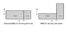
工学設計における本発明者らの現在の応用を含む、実用的な問題における代わりの目標は、正確な重みを持つ事象の派生物よりもむしろ、多くの希少で致命的な事象を発見することである。これは、図6に示されるように、致命的な事象の領域[Cth,Cmax]を他の領域[Cmin,Cth]よりも重点的に扱うことによって効率的に達成され得る。次の解析は、事象空間Sを全体にまんべんなく探索することなく、致命的な事象が観察される範囲を集中的にもっとも効率的に減らすことを示し、それによって致命的な事象上を重点的に扱う。
[最適な提案分布]
十分に緩和されたMCMCプロセスは詳細釣り合いを満たし、生成された事象Xは定常状態になっている。従って、最適な提案分布Q(C(X))の条件は、効率的に発生されるべき致命的な事象を、MCMCプロセスの単一の遷移工程の解析から推測するのを可能にする。
十分に緩和されたMCMCプロセスは詳細釣り合いを満たし、生成された事象Xは定常状態になっている。従って、最適な提案分布Q(C(X))の条件は、効率的に発生されるべき致命的な事象を、MCMCプロセスの単一の遷移工程の解析から推測するのを可能にする。
本発明者らの目標の致命的な事象は、上記[実験結果]において本発明者らの解析によって論証されたように、事象空間Sに属する多数の領域に位置付けられるのであるから、事象空間SはS=R∪/Rとしてモデル化され得る。ここで、Rは、次の数15

で表され、全てのi≠j、j、j=1、・・・、rに対して、Ri∩Rj=0であり、/R=S\Rである。Riは、致命的な事象の集合であり、/Rは、非致命的な事象の集合である。ここで、簡単のためのメタ事象として各事象集合を参照する。各致命的なメタ事象Riは、十分に特定の場所に局在化されており、他の致命的なメタ事象から十分に分離されているとする。
Q(Y’|Y)を、提案分布Q(X)に従う事象を生成するMCMCプロセスにおいて、メタ事象Yから他のメタ事象Y’への事象Xの遷移確率であると仮定する。上記仮定より、さらに任意の致命的なメタ事象の間の離散遷移は無視されると仮定する。したがって、すべてのRiと/Rとの間の非零の遷移確率のみを考察する。次の条件は、総合のメタ事象確率の状態とRiと/Rとの間の詳細釣り合いによって保持する。


任意の希少で致命的な事象を見過ごすのを避けるための最も効率的方法において事象空間Sを考察することは、トータルとしてRiと/Rとの間の最も大きい遷移確率を要求する。

数16を置換し、Q(Ri)によって微分することよって、最大値に対して次の条件を得る。

さらにこの式を数17に置換し、すべてのiでの合計をとり、数16の制約を適用することによって、次の簡単な条件を得る。

この結果は、Q(R)=Q(/R)=0.5、すなわち、次の数21を導き出す。

Q(C(X))の一様な分布は任意の統計推定の最小偏差を提供するので、上の条件を満足している間、それぞれ、Riと/Rとで一定である、Q(C(X))の次の目標ヒストグラムを使用する。

致命的な事象を規定するために与えられる、Cthは、[Cmin,Cmax]の上限に一般的に近いので、致命的な事象用のQ(C(X))の値は、非致命的な事象用のそれよりも大きい。
[Focused Multicanonical MCMC法]
前の[最適な提案分布]において与えられた結果に基づいて、本発明者らは、希少で致命的な事象を効率的に発見するために、「Focused Multicanonical MCMC法」と名づけられた、Multicanonical MCMC法の拡張を提案する。上記表1のAlgorithm 1において、Q(Ci)、i=1、・・・、Bが収束するために必要な目的のヒストグラムの形は、フラットではなく、数22によって与えられる階段関数状である。この変更を除いて、上記アルゴリズムに他の変更は必要ない。
前の[最適な提案分布]において与えられた結果に基づいて、本発明者らは、希少で致命的な事象を効率的に発見するために、「Focused Multicanonical MCMC法」と名づけられた、Multicanonical MCMC法の拡張を提案する。上記表1のAlgorithm 1において、Q(Ci)、i=1、・・・、Bが収束するために必要な目的のヒストグラムの形は、フラットではなく、数22によって与えられる階段関数状である。この変更を除いて、上記アルゴリズムに他の変更は必要ない。
希少で致命的な事象P(R)の確率は、また、容易に計算される。数22におけるQ(C(X))の階段状ヒストグラムは、次の数23によって提供される。



数3、数23および数24を、数6に代入することによって、次の数26が得られる。
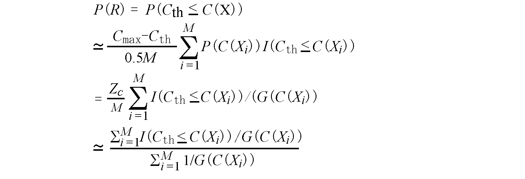

したがって、一度、G(C(Xi))がワン・ランダウ法によって得られると、希少で致命的な事象の確率P(R)は、標準的な方法と同様な方法で計算される。
[Focused Multicanonical MCMC法の実験結果]
図5(b)は、前述したように閾値Cth=0.6を使用した、本発明者らのFocused Multicanonical MCMC法におけるC(X)上でのサンプルされた事象のヒストグラムを示す。このヒストグラムは、階段状の形状をしており、閾値Cthでバランスされている。この収束を達成するための、シミュレーション実験の総数とそれらの計算時間は、それぞれ、6.1×10⁴と20.7時間であった。
図5(b)は、前述したように閾値Cth=0.6を使用した、本発明者らのFocused Multicanonical MCMC法におけるC(X)上でのサンプルされた事象のヒストグラムを示す。このヒストグラムは、階段状の形状をしており、閾値Cthでバランスされている。この収束を達成するための、シミュレーション実験の総数とそれらの計算時間は、それぞれ、6.1×10⁴と20.7時間であった。
図7は、標準的なMulticanonical MCMC法(sm-MCMC)と提案したFocused Multicanonical MCMC法(fm-MCMC)との間のヒストグラム更新上の迷光を引き起こす得られた光線の数の比較を示す。この図から容易に確認されるように、提案した方法によって希少迷光を得るための効率は、標準的なMulticanonical MCMC法のそれよりもほぼ2倍の高効率に収束する。
[他の方法との比較]
表2は、グリッドサーチ、ベイズ最適化、標準的なMulticanonical MCMC法、およびFocused Multicanonical MCMC法の性能比較を示す。グリッドサーチは、全体の事象空間の網羅探索アルゴリズムであって、ベースラインの性能を提供している。本発明者らは、遺伝的アルゴリズムと、シミュレーテッド・アニーシングを評価していない。何故なら、それらは膨大な数のシミュレーションを必要とすることによって実行不可能だからである。
表2は、グリッドサーチ、ベイズ最適化、標準的なMulticanonical MCMC法、およびFocused Multicanonical MCMC法の性能比較を示す。グリッドサーチは、全体の事象空間の網羅探索アルゴリズムであって、ベースラインの性能を提供している。本発明者らは、遺伝的アルゴリズムと、シミュレーテッド・アニーシングを評価していない。何故なら、それらは膨大な数のシミュレーションを必要とすることによって実行不可能だからである。

この表2の第1および第2の欄は、シミュレーション試験毎の希少で致命的な事象を発見する確率、すなわち、探索の効率を示す。第1の欄は、位置[x,y]を迷光を観察したところの位置に固定して、迷光を引き起こす入射光の方向[α,β]を探索するときの効率を示す。ベイズ最適化の効率は、グリッドサーチのそれよりも一桁高い大きさがあるのに対して、標準的なMulticanonical MCMC法およびFocused Multicanonical MCMC法の効率は二桁高い大きさがある。表2の第2の欄は、4次元空間の全体を探索するときの効率を示している。大きな探索空間のために、ベイズ最適化は、扱った105の試験数内において、いずれの致命的な事象を見つけることができなかった。これに対して、2つのMulticanonical MCMC法は、1000の試験数内で1つの希少で致命的な事象を成功裏に発見でき、この効率は、グリッドサーチよりも5桁高い大きさである。2次元および4次元の場合のいずれの場合においても、Focused Multicanonical MCMC法の効率は、標準的なMulticanonical MCMC法の2倍である。これらの結果は、[希少事象探索のために特殊化されたMulticanonical MCMC法]における議論に従っている。
表2の最後の欄は、希少で致命的な事象の確率P(R)の推定値、すなわち、迷光が起こるリスクを示している。グリッドサーチの推定値は、高い不確実性を含むことが予期される。何故なら、グリッドサーチは、迷光を引き起こす非常に制限された数の光線を発見できるだけで、したがって大きな統計的誤差を導くからである。ベイズ最適化は、この確率を提供できない。何故なら、それは、探索において確率的情報を保有しないからである。標準的なMulticanonical MCMC法およびFocused Multicanonical MCMC法の数8および数26は、グリッドサーチによって得られる確率と同じ位の大きさの持つ推定値を提供する。
図8は、上記光学系シミュレータSim(X)を用いる、本発明の第1の実施例による光学系設計支援システム100を示すブロック図である。光学系設計支援システム100は、図1に示すような、望遠鏡のような設計した光学系10において迷光が発生する可能性を発見するシステムである。
光学系設計支援システム100は、処理部200と、記憶部300とを備える。処理部200は、例えば、CPU(Central Processing Unit)などのプロセッサから成るが、これに限定されないのは勿論である。記憶部300は、例えば、RAM(random access memory)やROM(read only memory)などから成るが、これらに限定されないのは勿論である。
処理部200は、パラメータ決定部210と、軌跡算出部220と、評価値算出部230とを備える。記憶部300は、パラメータ記憶部310と、光学モデル記憶部320と、評価値記憶部330とを備える。
パラメータ決定部210は、後述するように、パラメータを決定する。パラメータ決定部210は、各パラメータとして、上述したように、設計した光学系10の受光面15における2次元の位置(x、y)および光線が受光面15に入光する2方向の角度(α、β)の計4次元の変数の組み合わせを決定する。パラメータ記憶部310は、決定したパラメータを記憶する。
軌跡算出部220は、決定したパラメータを使用して、後述するように、設計した光学系10における光線の軌跡を算出する。軌跡算出部220は、受光面15から入光口の方向に向けて、光線が逆伝播する軌跡を算出する。光学モデル記憶部320は、設計した光学系10における入光口から受光面15までの光路上に複数の光学部品を配置した光学モデルを記憶する。この光学モデルは、設計した光学系10に対応している。軌跡算出部220は、光学モデル記憶部320に記憶した光学モデルの入力を受け付け、光学モデルにおける光線の挙動を示す軌跡を算出する。
評価値算出部230は、算出した軌跡と、理想的な光学系においてパラメータのもとで期待される軌跡との比較に基づいて、パラメータに対して迷光が発生する可能性を示す評価値を算出する。換言すれば、評価値算出部230は、上記設計した光学系10(光学モデル)に応じて一意に規定される評価関数C(X)を持つ。すなわち、上記光学系シミュレータSim(X)は、評価関数C(X)を持つ。評価値算出部230は、算出した軌跡と決定したパラメータとを受け、評価関数C(X)に従って評価値を算出する。評価値記憶部330は、算出した評価値を記憶する。
したがって、パラメータ記憶部310は過去の軌跡の算出に使用したパラメータを記憶する。評価値記憶部330はそのパラメータに対して算出した評価値を記憶する。
パラメータ決定部210は、パラメータ記憶部310に記憶したパラメータおよび評価値記憶部330に記憶した評価値に基づいて、当該評価値が高いほどパラメータに近くなるように、次回以降の軌跡算出に使用するパラメータを決定する。
パラメータ決定部210は、評価値が高いほどパラメータに近い乱数が得られるような乱数の分布を定義し、この分布に基づいて次回以降の軌跡算出に使用するパラメータを生成する。
図9は、図8に使用されるパラメータ決定部210の構成を詳細に示すブロック図である。パラメータ決定部210は、ヒストグラム算出部212と、乱数分布定義部214と、パラメータ生成部216とから成る。
以下、図8および図9を参照して、光学系設計支援システム100の動作について更に詳細に説明する。
パラメータ記憶部310は、過去の軌跡の算出に使用したN個のパラメータを記憶する。
パラメータ決定部210は、上記分布に基づいて、次回以降N回の軌跡算出に使用するN個のパラメータをそれぞれ決定する。
軌跡算出部220は、決定したN個のパラメータに対してそれぞれN本の軌跡を算出する。
評価値算出部230は、決定したN個のパラメータおよび算出したN本の軌跡に対してそれぞれN個の評価値を算出する。評価値記憶部330は、N個のパラメータに対して算出されたN個の評価値を記憶する。
ヒストグラム算出部212は、パラメータ記憶部310から過去の軌跡の算出に使用したN個のパラメータを受け、評価値記憶部330からN個のパラメータに対して算出されたN個の評価値を受ける。ヒストグラム算出部212は、評価値を階級とし、各階級のパラメータの個数を度数とするヒストグラムを算出する。
乱数分布定義部214は、算出したヒストグラムに基づいて、次回以降N回の軌跡算出に使用するN個のパラメータを生成するための乱数の分布を、ヒストグラムが実質的に平坦になるような乱数が得られるように定義する(図6の左側の図参照)。
パラメータ生成部216は、定義した乱数の分布に従って、次回以降の各軌跡算出に使用する各パラメータを生成する。すなわち、パラメータ生成部216は、図5(a)に示されるように、ヒストグラムが実質的に平坦になるようにN個のパラメータを生成する。
したがって、パラメータ決定部210は、上記標準的なMulticanonical MCMC法を用いて次回以降N回の軌跡算出に使用するN個のパラメータを決定する。
より具体的に説明すると、ランダムに乱数(パラメータ)を発生すると、評価値としては、図2の左側の図のように、閾値Cth=0.6より小さい評価値のパラメータの度数が沢山得られることになる。そこで、パラメータ決定部210は、閾値Cth=0.6以上の評価値が得られる乱数(パラメータ)を全て採用するが、閾値Cth=0.6より小さい評価値が得られる乱数(パラメータ)についてはほとんどを破棄し、たまに採用することで、図2の右側の図のように、ヒストグラムが実質的に平坦になるようにN個のパラメータを決定する。
光学系設計支援システム100は、上記動作を複数回繰り返すことによって、図5(a)に示されるような、最終的にヒストグラムが実質的に平坦になるようにN個のパラメータを決定することができる。ここで、「実質的に平坦」とは、各階級における度数が、平均度数に対して所定の誤差の範囲内に入っていることを意味する。これを図5(a)の場合を例に挙げて説明する。平均度数が75であって、所定の誤差が15であるとする。この場合、各階級における度数は、60~90の範囲に入っている。
以上の説明から明らかなように、本第1の実施例によれば、光学系における迷光を自動的に確実に解析することができる。
図10は、上記光学系シミュレータSim(X)を用いる、本発明の第2の実施例による光学系設計支援システム100Aを示すブロック図である。光学系設計支援システム100Aも、図1に示すような、望遠鏡のような設計した光学系10において迷光が発生する可能性を発見するシステムである。
図示の光学系設計支援システム100Aは、処理部の構成および動作が後述するように相違する点を除いて、図8に示した光学系設計支援システム100と同様の構成を有し動作をする。従って、処理部に200Aの参照符号を付している。図8に示されたものと同様の機能を有するものには同一の参照符号を付して、説明の簡略化のためにそれらについて説明を省略する。
処理部200Aは、パラメータ決定部の構成および動作が後述するように相違する点を除いて、図8に示した処理部200と同様の構成を有し動作をする。従って、パラメータ決定部に210Aの参照符号を付している。
図11は、図10の光学系設計支援システム100Aに使用されるパラメータ決定部210Aの構成を詳細に示すブロック図である。パラメータ決定部210Aは、乱数分布定義部の構成および動作が後述するように相違する点を除いて、図9に示したパラメータ決定部210と同様の構成を有し動作をする。従って、乱数分布定義部に214Aの参照符号を付している。
乱数分布定義部214Aは、算出したヒストグラムに基づいて、次回以降N回の軌跡算出に使用するN個のパラメータを生成するための乱数の分布を、ヒストグラムの階級に対して定められた閾値Cth以上の各階級でのパラメータの度数が閾値Cth以下の各階級におけるパラメータの度数よりも高いようなヒストグラムを与える乱数が得られるように、定義する。
尚、図示の例では、ヒストグラムの階級の最大値が1.0となるように正規化されており、閾値Cthは0.6に等しい。
乱数分布定義部214Aは、ヒストグラムの階級に対して定められた閾値Cth以上のパラメータの度数の合計と閾値Cth以下のパラメータの度数の合計とが実質的に等しくなるようなヒストグラムを与える乱数が得られるように、分布を定義する。ここで、「実質的に等しい」とは、所定の誤差の範囲内において、閾値Cth以上のパラメータの度数の合計と閾値Cth以下のパラメータの度数の合計とが等しいことを意味する。
パラメータ生成部216は、定義した乱数の分布に従って、図5(b)に示されるように、次回以降の各軌跡算出に使用する各パラメータを生成する。すなわち、パラメータ生成部216は、図5(b)に示されるように、ヒストグラムが、閾値Cth以上のパラメータの度数の合計と閾値Cth以下のパラメータの度数の合計とが実質的に等しくなるように、N個のパラメータを生成する。
したがって、パラメータ決定部210Aは、上記Focused Multicanonical MCMC法を用いて次回以降N回の軌跡算出に使用するN個のパラメータを決定する。
より具体的に説明すると、ランダムに乱数(パラメータ)を発生すると、評価値としては、図2の左側の図のように、閾値Cth=0.6より小さい評価値においてパラメータの度数の高いものが沢山得られることになる。そこで、パラメータ決定部210Aは、閾値Cth=0.6以上の評価値が得られる乱数(パラメータ)を全て採用するが、閾値Cth=0.6より小さい評価値が得られる乱数(パラメータ)についてはほとんどを破棄し、たまに採用する。このことにより、図5(b)に示されるように、パラメータ決定部210Aは、ヒストグラムが、閾値Cth以上のパラメータの度数の合計と閾値Cth以下のパラメータの度数の合計とが実質的に等しくなるようにN個のパラメータを決定する。
光学系設計支援システム100Aは、上記動作を複数回繰り返すことによって、図5(b)に示されるような、ヒストグラムが閾値Cth以上のパラメータの度数の合計と閾値Cth以下のパラメータの度数の合計とが実質的に等しくなるようにN個のパラメータを生成することができる。
なお、本例では、乱数分布定義部214Aは閾値Cthを0.6に設定しているが、乱数分布定義部214Aは、閾値Cthを0.5より大きい値に設定すればよい。但し、乱数分布定義部214Aは、閾値Cthを0.6以上0.8以下の範囲の間に設定することが好ましい。しかしながら、乱数分布定義部214Aは、閾値Cthを0.6の値に設定することがより好ましい。その理由は次の通りである。
一般に、迷光は1つだけであるとは限らず、上述した対称性等に起因して、複数個ある場合がほとんどである。そのような状況において、もし閾値Cthを0.8より高く設定してしまうと、その閾値Cthより小さい評価値の乱数(パラメータ)のほとんどが破棄されてしまい、他の迷光を探索できる可能性(確率)が非常に低くなってしまうからである。また、閾値Cthを0.6より低く設定しまうと、効率的に複数の迷光を探索できなくなってしまうからである。よって、閾値Cthを0.6の値に設定することが好ましい。
以上の説明から明らかなように、本第2の実施例によれば、光学系における複数の迷光を自動的に効率的に解析することができる。
図12は、本発明の第3の実施例による希少事象解析装置100Bを示すブロック図である。希少事象解析装置100Bは、希少事象が発生する可能性を発見する装置である。具体的には、希少事象解析装置100Bは、例えば、図1に示すような、望遠鏡のような設計した光学系10において発生する迷光を希少事象として発見する。しかしながら、希少事象解析装置100Bは、そのような設計した光学系10のシミュレーションだけでなく、他の目的系のシミュレーションにも適用され得る。
希少事象解析装置100Bは、処理部200Bと、記憶部300Bとを備える。処理部200Bは、例えば、CPU(Central Processing Unit)などのプロセッサから成るが、これに限定されないのは勿論である。記憶部300Bは、例えば、RAM(random access memory)やROM(read only memory)などから成るが、これらに限定されないのは勿論である。
処理部200Bは、パラメータ決定部210Bと、シミュレータ220Bと、評価値取得部230Bとを備える。記憶部300は、パラメータ記憶部310Bと、評価値記憶部330Bとを備える。
シミュレータ220Bは、例えば、上記光学系シミュレータSim(X)であってよい。この場合、シミュレータ220Bは、図8に示されている、光学モデル記憶部320と軌跡算出部220と評価値算出部230との組み合わせで実現され得る。しかしながら、シミュレータ220Bは、上記光学系シミュレータSim(X)には限定されず、他のシミュレータであってよい。シミュレータ220Bは、希少事象が発生する可能性を規定する評価関数C(X)を持つ。
パラメータ決定部210Bは、提案分布Q(X)に基づいて、毎回の試験k(1≦k≦K)におけるN回のシミュレーションに使用するN個のパラメータXkを決定する。N個のパラメータXkの各々は、事象を規定する。パラメータ決定部210Bは、N個のパラメータXkを1つずつ順次、シミュレータ220Bに供給する。パラメータ記憶部310Bは、決定したパラメータを記憶する。
評価値取得部230Bは、N個のパラメータXkに対応してシミュレータ220Bから出力されるN個の評価値C(Xk)を取得する。評価値記憶部330Bは、このN個の評価値を記憶する。
パラメータ記憶部310Bは、過去の試験(k-1)のN回のシミュレーションに使用したN個の過去のパラメータXk-1を記憶する。評価値記憶部330Bは、それらN個の過去のパラメータXk-1に対するN回のシミュレーションで取得されたN個の過去の評価値C(Xk-1)を記憶する。
パラメータ決定部210Bは、パラメータ記憶部310Bに記憶されているN個の過去のパラメータXk-1と、評価値記憶部330Bに記憶されているN個の過去の評価値C(Xk-1)とに基づいて、後述するように、今回の試験kにおけるN回のシミュレーションに使用するN個のパラメータXkを決定する。
図13は、図12に使用されるパラメータ決定部210Bの構成を詳細に示すブロック図である。パラメータ決定部210Bは、ヒストグラム算出部212Bと、乱数分布定義部214Bと、パラメータ生成部216Bとから成る。
ヒストグラム算出部212Bは、パラメータ記憶部310Bに記憶されたN個の過去のパラメータXk-1と、評価値記憶部330Bに記憶されたN個の過去の評価値C(Xk-1)とを受ける。ヒストグラム算出部212Bは、評価値を階級とし、各階級のパラメータの個数を度数とするヒストグラムを算出する。
乱数分布定義部214Bは、算出したヒストグラムに基づいて、今回の試験kのN回のシミュレーションに使用するN個のパラメータXkを生成するための乱数の分布を、ヒストグラムの階級に対して定められた閾値Cth以上の各階級でのパラメータの度数が、閾値Cth以下の各階級でのパラメータの度数よりも多くなるようなヒストグラムを与える乱数が得られるように、定義する。
尚、図示の例では、ヒストグラムの階級の最大値が1.0となるように正規化されており、閾値Cthは0.6に等しい。
乱数分布定義部214Bは、ヒストグラムの階級に対して定められた閾値Cth以上のパラメータの度数の合計と閾値Cth以下のパラメータの度数の合計とが実質的に等しくなるようなヒストグラムを与える乱数が得られるように、分布を定義する。ここで、「実質的に等しい」とは、所定の誤差の範囲内において、閾値Cth以上のパラメータの度数の合計と閾値Cth以下のパラメータの度数の合計とが等しいことを意味する。
パラメータ生成部216Bは、定義した乱数の分布に基づいて、図5(b)に示されるように、今回の試験kにおける各シミュレーションに使用する各パラメータXkを生成する。すなわち、パラメータ生成部216Bは、図5(b)に示されるように、ヒストグラムが、閾値Cth以上のパラメータの度数の合計と閾値Cth以下のパラメータの度数の合計とが実質的に等しくなるように、今回の試験kにおけるN回のシミュレーションに使用するN個のパラメータXkを生成する。
したがって、パラメータ決定部210Bは、上記Focused Multicanonical MCMC法を用いて、今回の試験kにおけるN回のシミュレーションに使用するN個のパラメータXkを決定する。
より具体的に説明すると、ランダムに乱数(パラメータ)を発生すると、評価値としては、図2の左側の図のように、閾値Cth=0.6より小さい評価値においてパラメータの度数の高いものが沢山得られることになる。そこで、パラメータ決定部210Bは、閾値Cth=0.6以上の評価値が得られる乱数(パラメータ)を全て採用するが、閾値Cth=0.6より小さい評価値が得られる乱数(パラメータ)についてはほとんどを破棄し、たまに採用する。このことにより、図5(b)に示されるように、パラメータ決定部210Bは、ヒストグラムが、閾値Cth以上のパラメータの度数の合計と閾値Cth以下のパラメータの度数の合計とが実質的に等しくなるように、今回の試験kにおけるN回のシミュレーションに使用するN個のパラメータXkを生成する。
希少事象解析装置100Bは、上記試験動作をK回繰り返すことによって、図5(b)に示されるような、ヒストグラムが閾値Cth以上のパラメータの度数の合計と閾値Cth以下のパラメータの度数の合計とが実質的に等しくなるように、最終回の試験Kにおいて、N個の最終のパラメータXKを生成することができる。
なお、本例では、乱数分布定義部214Bは閾値Cthを0.6に設定しているが、乱数分布定義部214Bは、閾値Cthを0.5より大きい値に設定すればよい。但し、乱数分布定義部214Bは、閾値Cthを0.6以上0.8以下の範囲の間に設定することが好ましい。しかしながら、乱数分布定義部214Bは、閾値Cthを0.6の値に設定することがより好ましい。その理由は次の通りである。
一般に、希少事象は1つだけであるとは限らず、複数個ある場合がほとんどである。そのような状況において、もし閾値Cthを0.8より高く設定してしまうと、その閾値Cthより小さい評価値(階級)の乱数(パラメータ)のほとんどが破棄されてしまい、他の希少事象を探索できる可能性(確率)が非常に低くなってしまうからである。また、閾値Cthを0.6より低く設定しまうと、効率的に複数の希少事象を探索できなくなってしまうからである。よって、閾値Cthを0.6の値に設定することが好ましい。
以上の説明から明らかなように、本第3の実施例によれば、目的系における複数の希少事象を自動的に効率的に解析することができる。
なお、本発明は、上記実施例そのままに限定されるものではなく、実施段階ではその要旨を逸脱しない範囲で構成要素を変形して具体化できる。また、複数の構成要素の適宜な組合せにより種々の発明を形成できる。
尚、光学系設計支援システム(希少事象解析装置)の各部は、ハードウェアとソフトウェアとの組み合わせを用いて実現すればよい。ハードウェアとソフトウェアとを組み合わせた形態では、RAM(random access memory)に光学系設計支援(希少事象解析)プログラムが展開され、該光学系設計支援(希少事象解析)プログラムに基づいて、CPU(central processing unit)等のプロセッサのハードウェアを動作させることによって、各部を各種手段として実現する。また、該光学系設計支援(希少事象解析)プログラムは、記録媒体に記録されて頒布されても良い。当該記録媒体に記録された光学系設計支援(希少事象解析)プログラムは、有線、無線、又は記録媒体そのものを介して、メモリに読込まれ、プロセッサ(CPU)等を動作させる。尚、記録媒体を例示すれば、オプティカルディスクや磁気ディスク、半導体メモリ装置、ハードディスクなどが挙げられる。
上記第1および第2の実施例を別の表現で説明すれば、光学系設計支援システムとして動作させるコンピュータを、RAMに展開された光学系設計支援プログラムに基づき、パラメータ決定部210、210A、軌跡算出部220、および評価値算出部230の組み合わせとして動作させることで、実現することが可能である。
上記第3の実施例を別の表現で説明すれば、希少事象解析装置として動作させるコンピュータを、RAMに展開された希少事象解析プログラムに基づき、パラメータ決定部210B、シミュレータ220B、および評価値取得部230Bの組み合わせとして動作させることで、実現することが可能である。
また、本発明の具体的な構成は前述の実施例に限られるものではなく、この発明の要旨を逸脱しない範囲の変更があってもこの発明に含まれる。
以上、実施の形態を参照して本願発明を説明したが、本願発明は上記実施例に限定されるものではない。本願発明の構成や詳細には、本願発明のスコープ内で当業者が理解し得る様々な変更をすることができる。
本発明は、光通信やカメラ等の光学系シミュレータと併用して利用可能である。また、本発明は、工学設計における終局条件探索のような他のシミュレータと併用しても利用可能である。
この出願は、2017年6月30日に出願された日本出願特願2017-129002を基礎とする優先権を主張し、その開示の全てをここに取り込む。
10 設計した光学系(望遠鏡)
11 第1の鏡
12 第2の鏡
13 第3の鏡
14 平面鏡
15 受光面
16 正規光の光路
17 迷光の光路
100、100A 光学系設計支援システム
100B 希少事象解析装置
200、200A、200B 処理部
210、210A パラメータ決定部
212、212B ヒストグラム算出部
214、214A、214B 乱数分布定義部
216、216B パラメータ生成部
220 軌跡算出部
220B シミュレータ
230 評価値算出部
230B 評価値取得部
300、300B 記憶部
310、310B パラメータ記憶部
320 光学モデル記憶部
330、330B 評価値記憶部
11 第1の鏡
12 第2の鏡
13 第3の鏡
14 平面鏡
15 受光面
16 正規光の光路
17 迷光の光路
100、100A 光学系設計支援システム
100B 希少事象解析装置
200、200A、200B 処理部
210、210A パラメータ決定部
212、212B ヒストグラム算出部
214、214A、214B 乱数分布定義部
216、216B パラメータ生成部
220 軌跡算出部
220B シミュレータ
230 評価値算出部
230B 評価値取得部
300、300B 記憶部
310、310B パラメータ記憶部
320 光学モデル記憶部
330、330B 評価値記憶部
Claims (7)
- 希少事象が発生する可能性を発見する希少事象解析装置であって、
提案分布Q(X)に基づいて、毎回の試験k(1≦k≦K)におけるN回のシミュレーションに使用する、各々が事象を規定するN個のパラメータXkを決定して、前記N個のパラメータXkを1つずつ順次、前記希少事象が発生する可能性を規定する評価関数C(X)を持つシミュレータに供給するパラメータ決定部と、
前記N個のパラメータXkに対応して、該当シミュレータから出力されるN個の評価値C(Xk)を取得する評価値取得部と、を備え、
前記パラメータ決定部は、過去の試験(k-1)のN回のシミュレーションに使用したN個の過去のパラメータXk-1と、該N個の過去のパラメータXk-1に対するN回のシミュレーションで取得されたN個の過去の評価値C(Xk-1)とに基づいて、今回の試験kにおけるN回のシミュレーションに使用するN個のパラメータXkを決定し、
前記パラメータ決定部は、
前記N個の過去のパラメータXk-1と前記N個の過去の評価値C(Xk-1)とを入力して、評価値を階級とし、各階級のパラメータの個数を度数とするヒストグラムを算出するヒストグラム算出部と、
該算出したヒストグラムに基づいて、前記今回の試験kにおけるN回のシミュレーションに使用するN個のパラメータXkを生成するための乱数の分布を、前記ヒストグラムの階級に対して定められた閾値Cth以上の各階級でのパラメータの度数が、前記閾値Cth以下の各階級でのパラメータの度数よりも多くなるようなヒストグラムを与える乱数が得られるように、定義する乱数分布定義部と、
該定義した乱数の分布に基づいて、前記今回の試験kにおける各シミュレーションに使用する各パラメータXkを生成するパラメータ生成部と、
を有する、希少事象解析装置。 - 前記乱数分布定義部は、前記ヒストグラムの階級に対して定められた閾値以上のパラメータの度数の合計と前記閾値以下のパラメータの度数の合計とが実質的に等しくなるようなヒストグラムを与える乱数が得られるように、前記分布を定義する、請求項1に記載の希少事象解析装置。
- 前記階級の最大値が1.0となるように正規化されている場合、前記乱数分布定義部は、前記閾値を0.5より大きい値に設定する、請求項2に記載の希少事象解析装置。
- 前記乱数分布定義部は、前記閾値を0.6以上0.8以下の範囲の間に設定する、請求項3に記載の希少事象解析装置。
- 前記乱数分布定義部は、前記閾値を0.6の値に設定する、請求項4に記載の希少事象解析装置。
- 希少事象が発生する可能性を発見する希少事象解析方法であって、
提案分布Q(X)に基づいて、毎回の試験k(1≦k≦K)におけるN回のシミュレーションに使用する、各々が事象を規定するN個のパラメータXkを決定して、前記N個のパラメータXkを1つずつ順次、前記希少事象が発生する可能性を規定する評価関数C(X)を持つシミュレータに供給する、パラメータを決定することと、
前記N個のパラメータXkに対応して、該シミュレータから出力されるN個の評価値C(Xk)を取得することと、を含み、
前記パラメータを決定することは、過去の試験(k-1)のN回のシミュレーションに使用したN個の過去のパラメータXk-1と、該N個の過去のパラメータXk-1に対するN回のシミュレーションで取得されたN個の過去の評価値C(Xk-1)とに基づいて、今回の試験kにおけるN回のシミュレーションに使用するN個のパラメータXkを決定することであり、
前記パラメータを決定することは、
前記N個の過去のパラメータXk-1と前記N個の過去の評価値C(Xk-1)とを入力して、評価値を階級とし、各階級のパラメータの個数を度数とするヒストグラムを算出することと、
該算出したヒストグラムに基づいて、前記今回の試験kにおけるN回のシミュレーションに使用するN個のパラメータXkを生成するための乱数の分布を、前記ヒストグラムの階級に対して定められた閾値Cth以上の各階級でのパラメータの度数が、前記閾値Cth以下の各階級でのパラメータの度数よりも多くなるようなヒストグラムを与える乱数が得られるように、定義することと、
該定義した乱数の分布に基づいて、前記今回の試験kにおける各シミュレーションに使用する各パラメータXkを生成することと、
を含む、希少事象解析方法。 - コンピュータに、希少事象が発生する可能性を発見する希少事象解析プログラムを記録した記録媒体であって、前記希少事象解析プログラムは、前記コンピュータに、
提案分布Q(X)に基づいて、毎回の試験k(1≦k≦K)におけるN回のシミュレーションに使用する、各々が事象を規定するN個のパラメータXkを決定して、前記N個のパラメータXkを1つずつ順次、前記希少事象が発生する可能性を規定する評価関数C(X)を持つシミュレータに供給するパラメータ決定手順と、
前記N個のパラメータXkに対応して、該シミュレータから出力されるN個の評価値C(Xk)を取得する評価値取得手順と、を実行させ、
前記パラメータ決定手順は、前記コンピュータに、過去の試験(k-1)のN回のシミュレーションに使用したN個の過去のパラメータXk-1と、該N個の過去のパラメータXk-1に対するN回のシミュレーションで取得されたN個の過去の評価値C(Xk-1)とに基づいて、今回の試験kにおけるN回のシミュレーションに使用するN個のパラメータXkを決定させるものであり、
前記パラメータ決定手順は、前記コンピュータに、
前記N個の過去のパラメータXk-1と前記N個の過去の評価値C(Xk-1)とを入力して、評価値を階級とし、各階級のパラメータの個数を度数とするヒストグラムを算出するヒストグラム算出手順と、
該算出したヒストグラムに基づいて、前記今回の試験kにおけるN回のシミュレーションに使用するN個のパラメータXkを生成するための乱数の分布を、前記ヒストグラムの階級に対して定められた閾値Cth以上の各階級でのパラメータの度数が、前記閾値Cth以下の各階級でのパラメータの度数よりも多くなるようなヒストグラムを与える乱数が得られるように、定義する乱数分布定義手順と、
該定義した乱数の分布に基づいて、前記今回の試験kにおける各シミュレーションに使用する各パラメータXkを生成するパラメータ生成手順と、
を実行させる、希少事象解析プログラム記録媒体。
Priority Applications (1)
| Application Number | Priority Date | Filing Date | Title |
|---|---|---|---|
| JP2019526651A JP6874239B2 (ja) | 2017-06-30 | 2018-05-08 | 希少事象解析装置、希少事象解析方法および希少事象解析プログラム記録媒体 |
Applications Claiming Priority (2)
| Application Number | Priority Date | Filing Date | Title |
|---|---|---|---|
| JP2017-129002 | 2017-06-30 | ||
| JP2017129002 | 2017-06-30 |
Publications (1)
| Publication Number | Publication Date |
|---|---|
| WO2019003644A1 true WO2019003644A1 (ja) | 2019-01-03 |
Family
ID=64742906
Family Applications (1)
| Application Number | Title | Priority Date | Filing Date |
|---|---|---|---|
| PCT/JP2018/017755 Ceased WO2019003644A1 (ja) | 2017-06-30 | 2018-05-08 | 希少事象解析装置、希少事象解析方法および希少事象解析プログラム記録媒体 |
Country Status (2)
| Country | Link |
|---|---|
| JP (1) | JP6874239B2 (ja) |
| WO (1) | WO2019003644A1 (ja) |
Cited By (1)
| Publication number | Priority date | Publication date | Assignee | Title |
|---|---|---|---|---|
| WO2020153495A1 (ja) * | 2019-01-24 | 2020-07-30 | 日本電気株式会社 | 探索装置、探索システム、探索方法および記録媒体 |
Citations (2)
| Publication number | Priority date | Publication date | Assignee | Title |
|---|---|---|---|---|
| JPH09107370A (ja) * | 1995-08-08 | 1997-04-22 | Toshiba Corp | シミュレーション方法およびシミュレータ |
| US20090248387A1 (en) * | 2008-03-28 | 2009-10-01 | Carnegie Mellon University | Method and apparatus for sampling and predicting rare events in complex electronic devices, circuits and systems |
Family Cites Families (1)
| Publication number | Priority date | Publication date | Assignee | Title |
|---|---|---|---|---|
| JPH1022356A (ja) * | 1996-07-02 | 1998-01-23 | Sony Corp | デバイスシミュレーション方法 |
-
2018
- 2018-05-08 JP JP2019526651A patent/JP6874239B2/ja active Active
- 2018-05-08 WO PCT/JP2018/017755 patent/WO2019003644A1/ja not_active Ceased
Patent Citations (2)
| Publication number | Priority date | Publication date | Assignee | Title |
|---|---|---|---|---|
| JPH09107370A (ja) * | 1995-08-08 | 1997-04-22 | Toshiba Corp | シミュレーション方法およびシミュレータ |
| US20090248387A1 (en) * | 2008-03-28 | 2009-10-01 | Carnegie Mellon University | Method and apparatus for sampling and predicting rare events in complex electronic devices, circuits and systems |
Non-Patent Citations (1)
| Title |
|---|
| KISAMORI, KEIICHI ET AL.: "Integration of machine learning and simulation", JOURNAL OF THE JAPAN SOCIETY FOR COMPUTATIONAL ENGINEERING AND SCIENCE, vol. 22, no. 2, 30 April 2017 (2017-04-30), pages 3587 - 3591 * |
Cited By (3)
| Publication number | Priority date | Publication date | Assignee | Title |
|---|---|---|---|---|
| WO2020153495A1 (ja) * | 2019-01-24 | 2020-07-30 | 日本電気株式会社 | 探索装置、探索システム、探索方法および記録媒体 |
| JPWO2020153495A1 (ja) * | 2019-01-24 | 2021-12-02 | 日本電気株式会社 | 探索装置、探索システム、探索方法およびプログラム |
| JP7185853B2 (ja) | 2019-01-24 | 2022-12-08 | 日本電気株式会社 | 探索装置、探索システム、探索方法およびプログラム |
Also Published As
| Publication number | Publication date |
|---|---|
| JP6874239B2 (ja) | 2021-05-19 |
| JPWO2019003644A1 (ja) | 2019-12-12 |
Similar Documents
| Publication | Publication Date | Title |
|---|---|---|
| Gillet et al. | Deep learning from 21-cm tomography of the cosmic dawn and reionization | |
| Sabih et al. | Utilizing explainable AI for quantization and pruning of deep neural networks | |
| Tewes et al. | Weak-lensing shear measurement with machine learning-Teaching artificial neural networks about feature noise | |
| Lee et al. | Quantum-inspired multi-parameter adaptive Bayesian estimation for sensing and imaging | |
| Su et al. | Gaussian process machine-learning method for structural reliability analysis | |
| Carvalho et al. | Decoding neutron star observations: Revealing composition through Bayesian neural networks | |
| JP2008310828A (ja) | 電気光学画像システムのエンドツーエンド設計 | |
| JP6874238B2 (ja) | 光学系設計支援システム、光学系設計支援方法および光学系設計支援プログラム | |
| Bülte et al. | Probabilistic neural operators for functional uncertainty quantification | |
| JP2014081216A (ja) | 波面光学測定装置 | |
| Foldager et al. | On the role of model uncertainties in Bayesian optimisation | |
| Krippendorf et al. | The eROSITA Final Equatorial-Depth Survey (eFEDS): A machine learning approach to inferring galaxy cluster masses from eROSITA X-ray images | |
| Kumar et al. | Modeling submillimeter galaxies in cosmological simulations: Contribution to the cosmic star formation density and predictions for future surveys | |
| Balabanov et al. | Bayesian posterior approximation with stochastic ensembles | |
| Dahlqvist et al. | Auto-RSM: An automated parameter-selection algorithm for the RSM map exoplanet detection algorithm | |
| JP6874239B2 (ja) | 希少事象解析装置、希少事象解析方法および希少事象解析プログラム記録媒体 | |
| Guo et al. | An objective reduction algorithm using representative Pareto solution search for many-objective optimization problems | |
| Xu | Hybrid adaptive sequential sampling for reliability-based design optimization | |
| Kuntzer et al. | Detecting unresolved binary stars in Euclid VIS images | |
| Bom et al. | Deep learning in wide-field surveys: Fast analysis of strong lenses in ground-based cosmic experiments | |
| US12573193B2 (en) | Spatial mode processing for high-resolution imaging | |
| CN121014095A (zh) | 参数生成方法和离子注入机 | |
| Weddell et al. | Wavefront prediction with reservoir computing for minimizing the effects of angular anisoplanatism | |
| Bom et al. | Bayesian Deep Learning for Shower Parameter Reconstruction in Water Cherenkov Detectors | |
| Ntampaka et al. | The velocity distribution function of galaxy clusters as a cosmological probe |
Legal Events
| Date | Code | Title | Description |
|---|---|---|---|
| 121 | Ep: the epo has been informed by wipo that ep was designated in this application |
Ref document number: 18825416 Country of ref document: EP Kind code of ref document: A1 |
|
| ENP | Entry into the national phase |
Ref document number: 2019526651 Country of ref document: JP Kind code of ref document: A |
|
| NENP | Non-entry into the national phase |
Ref country code: DE |
|
| 122 | Ep: pct application non-entry in european phase |
Ref document number: 18825416 Country of ref document: EP Kind code of ref document: A1 |