WO2016107876A1 - Vehicular motion monitoring method - Google Patents
Vehicular motion monitoring method Download PDFInfo
- Publication number
- WO2016107876A1 WO2016107876A1 PCT/EP2015/081361 EP2015081361W WO2016107876A1 WO 2016107876 A1 WO2016107876 A1 WO 2016107876A1 EP 2015081361 W EP2015081361 W EP 2015081361W WO 2016107876 A1 WO2016107876 A1 WO 2016107876A1
- Authority
- WO
- WIPO (PCT)
- Prior art keywords
- feature vector
- feature
- motion
- indicator
- vector
- Prior art date
Links
- 230000033001 locomotion Effects 0.000 title claims abstract description 66
- 238000000034 method Methods 0.000 title claims abstract description 53
- 238000012544 monitoring process Methods 0.000 title claims abstract description 14
- 239000013598 vector Substances 0.000 claims abstract description 155
- 230000002547 anomalous effect Effects 0.000 claims abstract description 19
- 238000013507 mapping Methods 0.000 claims abstract description 11
- 238000004364 calculation method Methods 0.000 claims abstract description 6
- 238000012502 risk assessment Methods 0.000 claims abstract description 4
- 239000000872 buffer Substances 0.000 claims description 51
- 230000006870 function Effects 0.000 claims description 31
- 125000004122 cyclic group Chemical group 0.000 claims description 30
- 230000001133 acceleration Effects 0.000 claims description 23
- 230000036461 convulsion Effects 0.000 claims description 12
- 230000004927 fusion Effects 0.000 claims description 9
- 230000002159 abnormal effect Effects 0.000 claims description 7
- 230000005540 biological transmission Effects 0.000 claims description 4
- 238000012935 Averaging Methods 0.000 claims description 2
- 238000013213 extrapolation Methods 0.000 claims description 2
- 238000001914 filtration Methods 0.000 claims description 2
- 238000005070 sampling Methods 0.000 claims description 2
- 238000012549 training Methods 0.000 description 17
- 230000008569 process Effects 0.000 description 10
- 230000006399 behavior Effects 0.000 description 7
- 230000006866 deterioration Effects 0.000 description 5
- 230000000694 effects Effects 0.000 description 5
- 230000008901 benefit Effects 0.000 description 4
- 239000011159 matrix material Substances 0.000 description 4
- 238000013459 approach Methods 0.000 description 3
- 238000004891 communication Methods 0.000 description 3
- 230000002035 prolonged effect Effects 0.000 description 3
- 238000004458 analytical method Methods 0.000 description 2
- 238000013500 data storage Methods 0.000 description 2
- 230000001419 dependent effect Effects 0.000 description 2
- 238000001514 detection method Methods 0.000 description 2
- 230000007613 environmental effect Effects 0.000 description 2
- 239000000446 fuel Substances 0.000 description 2
- 238000013485 heteroscedasticity test Methods 0.000 description 2
- 230000000116 mitigating effect Effects 0.000 description 2
- 230000001360 synchronised effect Effects 0.000 description 2
- 238000012360 testing method Methods 0.000 description 2
- 230000007704 transition Effects 0.000 description 2
- 238000007476 Maximum Likelihood Methods 0.000 description 1
- 241001274660 Modulus Species 0.000 description 1
- 206010041349 Somnolence Diseases 0.000 description 1
- 230000002411 adverse Effects 0.000 description 1
- 238000013528 artificial neural network Methods 0.000 description 1
- 230000009286 beneficial effect Effects 0.000 description 1
- 230000001186 cumulative effect Effects 0.000 description 1
- 230000007423 decrease Effects 0.000 description 1
- 230000003247 decreasing effect Effects 0.000 description 1
- 238000011161 development Methods 0.000 description 1
- 238000010586 diagram Methods 0.000 description 1
- 238000005315 distribution function Methods 0.000 description 1
- 230000009189 diving Effects 0.000 description 1
- 238000011156 evaluation Methods 0.000 description 1
- 230000003116 impacting effect Effects 0.000 description 1
- 230000010354 integration Effects 0.000 description 1
- 238000002955 isolation Methods 0.000 description 1
- 238000010801 machine learning Methods 0.000 description 1
- 238000007726 management method Methods 0.000 description 1
- 230000007246 mechanism Effects 0.000 description 1
- 238000012986 modification Methods 0.000 description 1
- 230000004048 modification Effects 0.000 description 1
- 230000035515 penetration Effects 0.000 description 1
- 238000001556 precipitation Methods 0.000 description 1
- 238000012887 quadratic function Methods 0.000 description 1
- 238000010223 real-time analysis Methods 0.000 description 1
- 238000011160 research Methods 0.000 description 1
Classifications
-
- B—PERFORMING OPERATIONS; TRANSPORTING
- B60—VEHICLES IN GENERAL
- B60W—CONJOINT CONTROL OF VEHICLE SUB-UNITS OF DIFFERENT TYPE OR DIFFERENT FUNCTION; CONTROL SYSTEMS SPECIALLY ADAPTED FOR HYBRID VEHICLES; ROAD VEHICLE DRIVE CONTROL SYSTEMS FOR PURPOSES NOT RELATED TO THE CONTROL OF A PARTICULAR SUB-UNIT
- B60W40/00—Estimation or calculation of non-directly measurable driving parameters for road vehicle drive control systems not related to the control of a particular sub unit, e.g. by using mathematical models
- B60W40/08—Estimation or calculation of non-directly measurable driving parameters for road vehicle drive control systems not related to the control of a particular sub unit, e.g. by using mathematical models related to drivers or passengers
- B60W40/09—Driving style or behaviour
-
- B—PERFORMING OPERATIONS; TRANSPORTING
- B60—VEHICLES IN GENERAL
- B60W—CONJOINT CONTROL OF VEHICLE SUB-UNITS OF DIFFERENT TYPE OR DIFFERENT FUNCTION; CONTROL SYSTEMS SPECIALLY ADAPTED FOR HYBRID VEHICLES; ROAD VEHICLE DRIVE CONTROL SYSTEMS FOR PURPOSES NOT RELATED TO THE CONTROL OF A PARTICULAR SUB-UNIT
- B60W50/00—Details of control systems for road vehicle drive control not related to the control of a particular sub-unit, e.g. process diagnostic or vehicle driver interfaces
- B60W2050/0001—Details of the control system
- B60W2050/0019—Control system elements or transfer functions
- B60W2050/0028—Mathematical models, e.g. for simulation
-
- B—PERFORMING OPERATIONS; TRANSPORTING
- B60—VEHICLES IN GENERAL
- B60W—CONJOINT CONTROL OF VEHICLE SUB-UNITS OF DIFFERENT TYPE OR DIFFERENT FUNCTION; CONTROL SYSTEMS SPECIALLY ADAPTED FOR HYBRID VEHICLES; ROAD VEHICLE DRIVE CONTROL SYSTEMS FOR PURPOSES NOT RELATED TO THE CONTROL OF A PARTICULAR SUB-UNIT
- B60W50/00—Details of control systems for road vehicle drive control not related to the control of a particular sub-unit, e.g. process diagnostic or vehicle driver interfaces
- B60W2050/0062—Adapting control system settings
- B60W2050/0075—Automatic parameter input, automatic initialising or calibrating means
-
- B—PERFORMING OPERATIONS; TRANSPORTING
- B60—VEHICLES IN GENERAL
- B60W—CONJOINT CONTROL OF VEHICLE SUB-UNITS OF DIFFERENT TYPE OR DIFFERENT FUNCTION; CONTROL SYSTEMS SPECIALLY ADAPTED FOR HYBRID VEHICLES; ROAD VEHICLE DRIVE CONTROL SYSTEMS FOR PURPOSES NOT RELATED TO THE CONTROL OF A PARTICULAR SUB-UNIT
- B60W2420/00—Indexing codes relating to the type of sensors based on the principle of their operation
- B60W2420/90—Single sensor for two or more measurements
- B60W2420/905—Single sensor for two or more measurements the sensor being an xyz axis sensor
-
- B—PERFORMING OPERATIONS; TRANSPORTING
- B60—VEHICLES IN GENERAL
- B60W—CONJOINT CONTROL OF VEHICLE SUB-UNITS OF DIFFERENT TYPE OR DIFFERENT FUNCTION; CONTROL SYSTEMS SPECIALLY ADAPTED FOR HYBRID VEHICLES; ROAD VEHICLE DRIVE CONTROL SYSTEMS FOR PURPOSES NOT RELATED TO THE CONTROL OF A PARTICULAR SUB-UNIT
- B60W2520/00—Input parameters relating to overall vehicle dynamics
- B60W2520/06—Direction of travel
-
- B—PERFORMING OPERATIONS; TRANSPORTING
- B60—VEHICLES IN GENERAL
- B60W—CONJOINT CONTROL OF VEHICLE SUB-UNITS OF DIFFERENT TYPE OR DIFFERENT FUNCTION; CONTROL SYSTEMS SPECIALLY ADAPTED FOR HYBRID VEHICLES; ROAD VEHICLE DRIVE CONTROL SYSTEMS FOR PURPOSES NOT RELATED TO THE CONTROL OF A PARTICULAR SUB-UNIT
- B60W2520/00—Input parameters relating to overall vehicle dynamics
- B60W2520/10—Longitudinal speed
- B60W2520/105—Longitudinal acceleration
-
- B—PERFORMING OPERATIONS; TRANSPORTING
- B60—VEHICLES IN GENERAL
- B60W—CONJOINT CONTROL OF VEHICLE SUB-UNITS OF DIFFERENT TYPE OR DIFFERENT FUNCTION; CONTROL SYSTEMS SPECIALLY ADAPTED FOR HYBRID VEHICLES; ROAD VEHICLE DRIVE CONTROL SYSTEMS FOR PURPOSES NOT RELATED TO THE CONTROL OF A PARTICULAR SUB-UNIT
- B60W2520/00—Input parameters relating to overall vehicle dynamics
- B60W2520/12—Lateral speed
- B60W2520/125—Lateral acceleration
-
- B—PERFORMING OPERATIONS; TRANSPORTING
- B60—VEHICLES IN GENERAL
- B60W—CONJOINT CONTROL OF VEHICLE SUB-UNITS OF DIFFERENT TYPE OR DIFFERENT FUNCTION; CONTROL SYSTEMS SPECIALLY ADAPTED FOR HYBRID VEHICLES; ROAD VEHICLE DRIVE CONTROL SYSTEMS FOR PURPOSES NOT RELATED TO THE CONTROL OF A PARTICULAR SUB-UNIT
- B60W2556/00—Input parameters relating to data
- B60W2556/10—Historical data
-
- B—PERFORMING OPERATIONS; TRANSPORTING
- B60—VEHICLES IN GENERAL
- B60W—CONJOINT CONTROL OF VEHICLE SUB-UNITS OF DIFFERENT TYPE OR DIFFERENT FUNCTION; CONTROL SYSTEMS SPECIALLY ADAPTED FOR HYBRID VEHICLES; ROAD VEHICLE DRIVE CONTROL SYSTEMS FOR PURPOSES NOT RELATED TO THE CONTROL OF A PARTICULAR SUB-UNIT
- B60W2556/00—Input parameters relating to data
- B60W2556/45—External transmission of data to or from the vehicle
- B60W2556/50—External transmission of data to or from the vehicle for navigation systems
Definitions
- the invention generally relates to monitoring vehicular motion and assessing the riskiness of the driving style.
- the first application field is (car) fleet management, where real-time information on the driving behaviour may be used in taking measures aiming at motivating the drivers to adopt a more efficient driving style, to reduce their energy footprint and to save fuel. On the scale of the fleets, significant savings in terms of CO2 emissions and fleet depreciation may be achieved.
- the second important application field is the car insurance market. The calculation of car insurance premium may be enriched by or exclusively be based on individual parameters like the covered distance, the time spent on the road, the time of day, the roads used, etc.
- Pay-As-You-Drive PAYD
- UBI Usage-Based Insurance
- a first aspect of the invention relates to a vehicular motion monitoring method comprising:
- a riskiness indicator (a numerical score representing riskiness) to each feature vector, the calculation of the riskiness indicator being based upon an event severity indicator (or severity score) indicative of how anomalous each feature vector is in comparison to the modelled population and upon a position of the feature vector relative to one or more previous and/or subsequent feature vectors;
- the method according to the first aspect of the invention has, amongst others, the advantage that the severity of each event can be determined with a relatively small computational effort using the determinative parameters of the multivariate Gaussian probability density function (i.e. typically using the feature's mean and the covariance matrix). The discrete values of the collected feature vectors need not be used for the computation of the severity indicator.
- the severity indicator basically measures how unusual (anomalous) a driving situation (event) is. Due to the fact that newly collected feature vectors are used to update the model, the method progressively adapts itself to an individual's driving style. Past approaches relied on fixed thresholds to detect risky driving maneuvers. One of their shortcomings thus was that differences in the vehicles' performance and mechanical characteristics have an impact on the results. The present method is considered to provide a fairer and more representative assessment of an individual's driving style. [9] In the context of the present document, the following definitions apply.
- Vehicle designates an automobile road vehicle (e.g. a car, a bus or a truck).
- “Longitudinal” and “lateral” are used with implicit reference to the frame of the vehicle: “longitudinal” means along the direction that the vehicle's front is pointing; “lateral” means the direction from the left to the right of the vehicle (or vice versa).
- the term "determinative parameters" of a multivariate Gaussian probability density function designates any set of parameters that completely defines the multivariate Gaussian probability density function.
- the typical set of determinative parameters consists of the mean value (or barycenter) of the modelled population and the (elements of) the covariance matrix. It should be noted, however, that other (mathematically equivalent) sets of determinative parameters could be used as well.
- a "set of motion observations" that is mapped on a feature vector designates motion observations that relate to essentially the same moment in time, i.e. that belongs to a time interval the duration of which is the inverse of the refresh rate of the feature vectors.
- "Speed" means the (scalar) longitudinal velocity.
- updating the determinative parameters of the multivariate Gaussian probability density function comprises entering each feature vector into a buffer memory so as to update the population of collected feature vectors and recalculating the determinative parameters.
- Each set of motion observations preferably comprises a speed (v) observation, to which the respective feature vector is associated through the mapping.
- the buffer memory preferably comprises a plurality of cyclic buffers, of which each contains a sub-population of the collected feature vectors corresponding to a specific speed range.
- entering a feature vector into the buffer memory comprises entering the feature vector into the cyclic buffer that corresponds to the speed range, which the speed observation associated with the feature vector belongs to.
- Dynamically updating the population of collected feature vectors always bears the risk that the updated population is less representative of "ordinary" driving behaviour than the previous population. Prolonged monotonous driving on motorways, for instance, may lead to a narrowed population of feature vectors. In consequence, driving events following monotonous driving periods are more likely to be qualified as anomalous (i.e. to reach a higher severity score).
- the plurality of cyclic buffers helps to mitigate the deterioration problem.
- monotonous driving still leads to some loss of population diversity but this loss will typically be limited to one or two cyclic buffers, i.e. one or two speed categories. The remaining cyclic buffers remain essentially unaffected.
- the cyclic buffers may all be of the same size (i.e. contain the same number of collected feature vectors) or of different sizes. The latter option may be used to give more or less weight to specific speed categories. If this option should be implemented, care should be taken not to attribute too much relative weight to speed categories in which monotonous driving is particularly likely to occur.
- the severity indicator (or severity score) is calculated for each feature vector based on the determinative parameters of the multivariate Gaussian probability density function and a quantile threshold (Qiim) representative of a proportion of events considered anomalous.
- Qiim quantile threshold
- D(xi , X2) designates the Mahalanobis distance between two elements xi and X2 of the feature space
- the Mahalanobis distance is defined by:
- the quantile threshold may be fixed once for all and stored as a constant in the system implementing the method. Preferably, however, the quantile threshold is a monotonously varying function of the variance of the speed variation (or the variance of the longitudinal acceleration), such that a lower proportion of events are considered abnormal in case of low acceleration variance and a higher proportion of events are considered abnormal in case of high acceleration variance.
- the quantile threshold as a function of the acceleration variance may e.g. be stored in the system in the form of a lookup table. As will be appreciated, such a dynamic quantile threshold also contributes to the mitigation of effects caused by the deterioration of the diversity of the modelled population of feature vectors.
- the quantile threshold applied in the computation of the severity score is increased. More anomalous events are thus detected.
- the quantile threshold applied in the computation of the severity score is decreased. The system thus tends to detect less anomalous events.
- the variance of longitudinal acceleration might be expressed in a discrete-time system as the variance of the speed variation, i.e. the variance of the speed difference between subsequent time steps.
- the first vector component of the feature vector may be speed variation and the second vector component may be bearing variation.
- the first vector component is the product of speed variation ⁇ (longitudinal acceleration) and standard deviation of the modulus of jerk, noted o(j), and the second vector component is the product of bearing variation, noted Ab, and standard deviation of the modulus of jerk.
- jerk designates the derivative of the acceleration vector with respect to time.
- the speed variation and the bearing variation are preferably obtained through a GNSS receiver, while the jerk is preferably obtained by an accelerometer.
- the features (components of the feature vectors) will thus indicate whether there is constructive consensus between the GNSS data and the accelerometer data.
- the first vector component is the product of speed, speed variation and standard deviation of the norm of the jerk vector and the second vector component is the product of speed, bearing variation and standard deviation of the modulus of jerk.
- the products in this embodiment have the additional advantage of mitigating heteroscedasticity (i.e. heterogeneous variance) of the features.
- the Av o(j) term tends to exhibit lower variance at higher speeds than at lower speeds.
- the one or more sensors may be operated at the same or different acquisition rates.
- the sets of motion observations are preferably produced at the feature vector refresh rate by data fusion involving sampling and/or interpolation and/or extrapolation and/or filtering and/or averaging.
- Each sensor typically produces its data at a particular rate.
- Acceleration sensors may e.g. work at several tens of Hz or higher frequencies, whereas the data rate of GNSS navigators is typically of the order of 1 Hz.
- raw data arriving with lower rates may be upsampled while data arriving with higher rates may be downsampled.
- the fusion layer may also be used to process the data and to produce statistical data such as, e.g., variances, standard deviations, averages, etc. and other derived data such as, e.g., derivatives, ratios, products, moduluses, etc. Both the raw data and the data produced by the fusion layer are considered herein as motion observations.
- the motion observations are captured with at least one of a GNSS receiver (also: GNSS navigator), an accelerometer and a magnetometer.
- a GNSS receiver also: GNSS navigator
- an accelerometer also: GNSS navigator
- a magnetometer also: GNSS navigator
- the method according to the first aspect of the invention comprises the wireless transmission of at least the integrated riskiness indicator, e.g. to a data center. That transmission may be scheduled to recur at fixed times, after fixed time intervals, after each trip or after a defined distance travelled.
- the recipient of the data may e.g. be an insurance company, a fleet manager, a car leasing company, a social network, a public institution, etc.
- the transmitted data preferably include an identifier of the driver, the distance travelled during the integration period.
- One advantage of the method is that the amount of transmitted data may be kept very small. Furthermore, detailed information about specific driving events, the driver's location, the travel history, etc.
- any detailed logs are stored in an anonymized manner.
- a second aspect of the invention relates to a mobile electronic device application (an "app") comprising instructions, which, when executed by a processor of a mobile electronic device, such as, e.g. a smartphone, a tablet, a phablet, a notebook or the like, cause the mobile electronic device to carry out the method as described herein.
- a third aspect of the invention relates to a vehicular motion monitoring method comprising:
- mapping sets of motion observations onto a respective feature vector in a feature space, each set of motion observations corresponding to a driving event and comprising a speed observation, which the feature vector is associated to through the mapping;
- the buffer memory comprising a plurality of cyclic buffers, each cyclic buffer containing a sub-population of collected feature vectors corresponding to a specific speed range, and wherein entering the feature vector into the buffer memory comprises entering the feature vector into the cyclic buffer that corresponds to the speed range, which the speed observation of the feature vector belongs to.
- the vehicular motion monitoring method according to the third aspect of the invention does not necessarily comprise all limitations of the method according to the first aspect of the invention and could be claimed separately, e.g. via a divisional or continuation application.
- the vehicular motion monitoring method according to the third aspect of the invention may comprise one or more, but preferably not all, of the following characteristics I to V:
- the feature space is two-dimensional
- the feature vector has a first vector component representative of a longitudinal motion characteristic and a second vector component representative of a lateral motion characteristic;
- the probability density function is a multivariate Gaussian probability density function;
- a riskiness indicator (a numerical score representing riskiness) is assigned to each feature vector (or to each driving event), the calculation of the riskiness indicator being based upon an event severity indicator (or severity score) indicative of how anomalous each feature vector is in comparison to the modelled population and upon a position of the feature vector relative to one or more previous and/or subsequent feature vectors;
- the riskiness indicator is integrated over time (e.g. in a memory space allocated to that indicator) so that a risk assessment of the driving style of the driver of the vehicle is obtained.
- Particularly preferred combinations of characteristics I to V are: o I but not any one of II to V; o I and II but not any one of III to V; o III but not any one of I, II, IV and V; o III and at least one of I and II, but not at least one of IV and V; o IV but not any one of I, II, III and V; o IV and V but not at least one of I to III.
- entering a feature vector into the buffer memory comprises entering the feature vector into the cyclic buffer that corresponds to the speed range, which the speed observation associated with the feature vector belongs to.
- Dynamically updating the population of collected feature vectors always bears the risk that the updated population is less representative of "ordinary" driving behaviour than the previous population. Prolonged monotonous driving on motorways, for instance, may lead to a less diverse (and in that sense impoverished) population of feature vectors. In consequence, classifying driving events following monotonous driving periods may lead to different results than after diversified driving.
- the plurality of cyclic buffers helps to mitigate the deterioration problem.
- monotonous driving still leads to some loss of population diversity but this loss will typically be limited to one or two cyclic buffers, i.e. one or two speed categories. The remaining cyclic buffers remain essentially unaffected.
- the cyclic buffers may all be of the same size (i.e. contain the same number of collected feature vectors) or of different sizes. The latter option may be used to give more or less weight to specific speed categories. If this option should be implemented, care should be taken not to attribute too much relative weight to speed categories in which monotonous driving is particularly likely to occur.
- the step of classifying the driving event may comprise assigning the driving event to one of at least two riskiness categories.
- a crude classification would consist in classifying each driving event either as “safe” (or “unrisky” or the like) or “risky” (or “dangerous” or the like).
- a more subtle classification may be achieved by using one or more intermediate categories between those extremes. Classification could also rely on a severity score or a riskiness score as described above.
- Classification of a driving event may additionally be based upon data not necessarily (directly) related to vehicular motion, such as e.g. geographical position of the vehicle, time of day, weather conditions (temperature, precipitation, etc.), traffic conditions, speed limits and other traffic rules, etc. These additional data are preferably included into the feature vector. According to an advantageous embodiment of a method according to the third aspect of the invention, these additional data are used to take environmental conditions into account for classification of the driving events.
- the geographical position may e.g. be used to assign a higher severity score or riskiness score if a driving event occurred in a zone known to be particularly dangerous (based e.g. on accident statistics).
- Time of day or daylight information
- weather and traffic information could be used in a similar manner: somewhat risky driving events could be classified as even more risky if they occur at night time, in bad weather or in dense traffic. Cumulation of adverse environmental conditions preferably leads to a still higher riskiness class or score.
- Driving event classification could further be made dependent on the respect of traffic rules. If, for instance, it is detected that the vehicle is exceeding the speed limit an otherwise "unrisky" driving event could be classified as a (more) risky one.
- the vehicular motion monitoring method according to the third aspect of the invention is preferably implemented on a mobile (electronic) device, such as, e.g. a smartphone, a tablet, a phablet, a notebook or the like.
- a fourth aspect of the invention relates to a mobile electronic device application comprising instructions, which, when executed by a processor of a mobile electronic device, cause the mobile electronic device to carry out the method according to the third aspect of the invention.
- the vehicle is equipped with one or more assistant systems such as, e.g., a drowsiness detector, a lane departure warning assistant, a distance monitoring system (for monitoring the distance to a vehicle ahead), a traffic sign recognition system, a rain sensor, etc.
- assistant systems such as, e.g., a drowsiness detector, a lane departure warning assistant, a distance monitoring system (for monitoring the distance to a vehicle ahead), a traffic sign recognition system, a rain sensor, etc.
- the app is preferably configured to wirelessly connect the mobile device to the vehicle's onboard communication network or at least to attempt to establish such a connection, and in case of successful connection, listening to the messages of any assistant system installed on the vehicle.
- Fig. 1 is a schematic illustration of a mobile electronic device for running an app carrying out the method according to the first aspect of the invention
- Fig. 2 is a schematic flow chart of a preferred embodiment of the method
- Fig. 3 is an illustration of the conceptual structure of a buffer memory with several cyclic buffers storing each a sub-population of the collected feature vectors;
- Fig. 4 is a chart illustrating how the quantile threshold may be varied as a function of acceleration variance
- Fig. 5 is a chart illustrating severity scores obtained during test drives under controlled conditions
- Fig. 6 is a diagram of the evolution of the feature vectors during a slalom drive
- Fig. 7 is an illustration of the classification of driving events using normalized feature vectors
- Fig. 8 is a chart which compares two choices of features
- Fig. 9 is a schematic flow chart of a preferred embodiment of a method according to the third aspect of the invention.
- a multivariate normal (MVN) model is used to detect risky driving maneuvers and profile drivers. To the inventors' best knowledge, this is the first time an MVN approach is considered for driver profiling. While previous driver profiling methods considered high sensor outputs or pre-established patterns in order to declare a risky driving maneuver or event, given the heterogeneity of both mobile devices and vehicles, the inventors believe that a profiling system needs to adapt its parameters to each individual context.
- Traditional fixed threshold or supervised machine learning techniques e.g., neural networks or naive Bayes
- neural networks or naive Bayes may be suitable for designing such a driver profiling mechanism but require previous knowledge on the training samples, indicating the expected values of the input variables at the exact time a risky maneuver is performed. Then, the generation of such a training data set for risky driving maneuvers for different devices and vehicles becomes unfeasible in practice. Moreover, it cannot be a prerequisite of the application that the final users manually label risky driving maneuvers in a training phase.
- an MVN-based anomaly detection fits well with the problem to model.
- it provides a high flexibility by dynamically adapting to different driving conditions with recurring updates of its determinative parameters. Also, given that it does not require any preliminary knowledge on the driving events it has to detect, it can be applied to any type of vehicle and mobile device.
- the MVN model has many advantages over other approaches for anomaly detection: o There is no need to establish rule sets or thresholds to detect risky maneuvers.
- the probability of an observation enables the assessment of driver behaviour in a continuous or quasi-continuous fashion rather than binary classification (i.e., discerning merely between risky and non-risky driving events).
- the model can be estimated efficiently on a mobile phone or any other mobile electronic device and can be continuously retrained to improve the parameter estimates.
- the memory footprint may be held essentially constant in time, since the population of feature vectors may be stored in cyclic buffers. Also the computation time for the model fitting is bounded and the complexity does not increase over time.
- the model can represent covariance among features (which is expected to be seen in vehicular dynamics).
- Fig. 1 schematically illustrates a mobile electronic device 10, e.g. a smart phone, equipped with several sensors, in particular, a GNSS navigator 12, a three-axis acceleration sensor 14 and a three-axis magnetometer 16.
- the sensors are connected to the processor 18 of the mobile device 10.
- a communications module 20 allows the mobile device to establish and accept wireless connections.
- the mobile electronic device 10 may be used to execute an app that uses the data captured by the sensors 12, 14, and 16 to monitor vehicular motion and to assess the riskiness of the driving style in accordance with the present invention.
- FIG. 2 A flowchart illustrating a preferred embodiment of a method according to the invention is provided in Fig. 2. As illustrated, the mobile device collects input variables (motion observations) using the available sensors 12, 14 and 16.
- the motion observations are then transformed into respective elements (feature vectors) in a two- dimensional feature space that aims at representing the longitudinal and lateral axes of movement of the vehicle.
- feature vectors are stored in a training buffer.
- the feature vectors are accumulated in the training buffer until a critical size is reached and the first MVN model can be computed using e.g. the maximum likelihood estimator (MLE).
- MLE maximum likelihood estimator
- the app becomes fully operational and begins to determine the severity of driving events and to compute the riskiness indicator as detailed hereinafter.
- Newly arriving feature vectors continue to be collected in the training buffer and the MVN model adjusted in consequence, e.g. by using the above-mentioned MLE.
- the GNSS navigator 12 produces its data (position vector, velocity vector and time) typically at a rate of the order of 1 Hz, whereas the accelerometer 14 issues acceleration vectors at a significantly higher rate (typically 20 Hz to 50 Hz in smartphones) and the acquisition rate of the magnetometer lies typically in the range from 20 to 200 Hz.
- the raw data provided by the different sensors at the different rates are combined and synchronised by the processor.
- this corresponds to a fusion layer 22, as shown in Fig. 2.
- Data acquired from faster sensors are buffered between two consecutive inputs from the slowest sensor (in our example the navigator).
- Motion observations at the desired refresh rate (e.g. 10 Hz) are obtained by upsampling and downsampling data acquired at lower and higher rates, respectively.
- the fusion layer also makes available derived data.
- the motion observations made available at the desired refresh rate are: o(j) the standard deviation of the norm of the jerk vector.
- the jerk vector is computed as the derivative with respect to time of the acceleration vector output by the accelerometer 14.
- v the speed calculated based upon data from the navigator 12 (with interpolation)
- Each set of motion observations o ⁇ o(j), v, ⁇ , ⁇ ( ⁇ ), Ab ⁇ is then mapped onto an element (feature vector), x, of a two-dimensional feature space, X (x ⁇ X).
- feature vector has a first vector component (feature) representative of a longitudinal motion characteristic and a second vector component representative of a lateral motion characteristic, with the following properties: i) extreme values of the features represent risky or abnormal driving maneuvers, ii) feature distribution can be approximated by a Gaussian distribution.
- the mapping step is illustrated in Fig. 2 by step 24.
- the first feature is selected as the product of ⁇ and o(j) and the second feature is selected as the product of Ab and o(j):
- the MVN model can be defined by a multivariate Gaussian probability density function:
- the determinative parameters ⁇ and ⁇ are obtained through a training process (steps 26 and 28) in Fig. 2. [47] The training process is executed in parallel with the event assessment process, which includes computing the severity of events (step 30), computing the riskiness indicator (step 32) and integrating the riskiness indicator over time (step 34).
- the training process is preferably continuous but could also be intermittent.
- each feature vector obtained in the mapping step is fed to a buffer memory (step 26), in which a population of previously collected feature vectors is maintained.
- a multivariate Gaussian probability density function is fitted to the population using the MLE, which yields the determinative parameters ⁇ and ⁇ .
- the buffer memory comprises a plurality of cyclic buffers (represented as columns in Fig. 3). Each cyclic buffer contains a sub-population of the collected feature vectors corresponding to a specific speed range. In the illustrated example, there are 7 cyclic buffers, each corresponding to a speed range of 30 km/h. It is assumed that the entire speed range of the vehicle is covered by the buffers, otherwise the uppermost speed range may be open-ended. When a new feature vector is available, it is entered into the cyclic buffer that corresponds to the speed range of the speed observation v of the set of motion observations underlying the feature vector.
- a cyclic buffer is completely filled up, the newly added feature vector replaces or overwrites the oldest feature vector of that cyclic buffer.
- all cyclic buffers are of the same size, but that may be implemented differently. Prolonged monotonous driving may lead to an overly homogeneous population of feature vectors in one or two cyclic buffers. However, situations, in which the entire population of feature vectors (which is used for the computation of ⁇ and ⁇ ) would be degraded to an extent that it produces only meaningless results, are extremely unlikely due to the "isolation" of the cyclic buffers from each other. Monotonous driving still leads to some loss of population diversity on the scale of the entire population but the overall impact thereof on the severity score and on the riskiness score can be kept on a low level.
- a metric for the severity is computed.
- a cut-off quantile threshold, Qiim is proposed that marks the quantile limit between common observations and those that are considered to be anomalous.
- Qiim defines a cut-off probability value, piim, which can be used to classify the samples.
- pnm be the value of the model-dependent inverse cumulative distribution function (CDF) of Qiim
- Q(x) the (approximate) quantile of the feature transform x of observation o
- the severity indicator may be expressed as:
- the severity indicator s defines a normalised metric of how anomalous a set of motion observations o or the corresponding feature vector x is.
- Qiim is typically chosen in the range from 10 "5 to 10 "2 (1 %). Lower values of Qiim will result in in fewer feature vectors being considered anomalous (i.e. being assigned a severity score different from 0).
- Qiim may be a constant in the application but a way to dynamically vary Qnm will be presented further down in the text.
- a low quantile threshold of 10 "5 is assigned to feature vectors for a ⁇ ( ⁇ ) close to zero.
- Qiim remains 0.1 .
- Qiim as a function of ⁇ ( ⁇ ) is preferably stored as a lookup table in the app. For the computation of s(x), the applicable value of Qiim may thus be retrieved from that table.
- Fig. 5 illustrates severity scores obtained during test drives under controlled conditions. Phases of normal driving were alternated with phases of exceptionally stark accelerations and decelerations (shaded areas) both in longitudinal and lateral directions. The speed is shown in the top graph as a reference. The bottom graph illustrates the severity score as a function of time. It can be seen that the anomalous driving events could be reliably detected.
- the severity indicator indicates how anomalous an event is.
- a riskiness indicator is computed for each feature vector at step 32. In order to analyse riskiness, the evolution of the feature vectors over time is taken into account. [55] Using the severity metric s(x) defined above as well as the Mahalanobis distance D m , a risk function is defined by:
- Fig. 6 illustrates the evolution of the feature vectors over time during driving a slalom.
- the arrows show the transitions between consecutive feature vectors.
- the boundary separating ordinary from anomalous feature vectors is shown as a white line.
- the grey disks surrounding each feature vector have radii proportional to the corresponding riskiness indicator R(x).
- the slalom trace shows variance in both dimensions of the feature space, as it can be observed in the diagonal transition lines between subsequent observations This is because the driver needs to constantly adapt speed (i.e., accelerate and brake) in order to pass between two obstacles.
- the riskiness indicator is accumulated (integrated) over time (step 34 in Fig. 2), e.g. during a trip.
- the integrated riskiness indicator ⁇ £ ⁇ ( ⁇ : £) then serves as a basis for driver scoring.
- the integrated riskiness indicator is finally transmitted (step 36 in Fig. 2) to a data center, together with an identifier of the driver (and/or of the mobile device on which the app is executed) and further data, such as, e.g. the time and/or the distance over which was integrated.
- the scaled feature space may be divided into four
- the polar coordinate ⁇ of the scaled or normalized feature vectors z may be averaged over several (e.g. 4) consecutive events.
- the event category may be computed for every feature vector. Preferably, however, the event category is only calculated for anomalous events (having a nonzero severity score s).
- the app may be configured so as not to log the individual events.
- the integrated riskiness indicator ⁇ i R (Xi) will be transmitted without detailed information as to how the integrated score was reached.
- the app could be configured to log and transmit all events but that implies that a lot of data have to be processed, which are of little value.
- the app may be configured to log the anomalous events.
- the app could e.g. be configured to store and transmit the category of such events, their position and time, the severity score and the riskiness indicator. In that way, the relevant data can be transmitted to the data center while impacting the communication networks significantly less.
- maximum acceleration decreases with increasing speed. It follows that the statistical variance of ⁇ is lower at high speeds than at lower speeds.
- Av ⁇ a(j) and Ab ⁇ a(j) with the speed v that effect is compensated to some extent. This is illustrated in Fig.
- FIG. 9 A flowchart illustrating a further preferred embodiment of a method according to an aspect of the invention is provided in Fig. 9.
- the mobile device collects input variables (motion observations) using the sensors 1 12, 1 14 and 1 16.
- the motion observations are then transformed into respective elements (feature vectors) in a feature space that aims at representing characteristics of the movement of the vehicle.
- feature vectors are stored in a training buffer.
- the app is executed for the first time, the feature vectors are accumulated in the training buffer until a critical size is reached and the determinative parameters of a probability density function modelling the population can be computed using an appropriate estimator.
- the app becomes fully operational and begins to classify driving events as detailed hereinafter. Newly arriving feature vectors continue to be collected in the training buffer and the determinative parameters are adjusted in consequence.
- the raw data are provided by the sensors 1 12, 1 14, 1 16 at different rates, they are combined and synchronised by the processor.
- this corresponds to a fusion layer 122, as shown in Fig. 9.
- Data acquired from faster sensors are buffered between two consecutive inputs from the slowest sensor.
- Motion observations at the desired refresh rate are obtained by upsampling and downsampling data acquired at lower and higher rates, respectively.
- the fusion layer 122 also makes available derived data.
- Each set of motion observations corresponding to a driving event is mapped onto an element (feature vector), x, of a feature space, X (x ⁇ X).
- feature vector has one or more components corresponding to motion characteristics with the following properties: i) extreme values of the features represent risky or abnormal driving maneuvers, ii) feature distribution can be approximated by a parameterizable probability density function.
- the mapping step is illustrated in Fig. 9 by step 124.
- the determinative parameters of the probability density function are obtained through a training process (steps 126 and 128 in Fig. 9).
- the training process is executed in parallel with driving event classification (step 130).
- the training process is preferably continuous but could also be intermittent.
- each feature vector obtained in the mapping step is fed to a buffer memory (step 126), in which a population of previously collected feature vectors is maintained.
- a probability density function e.g. a multivariate Gaussian probability density function
- the feature vector population can be maintained as previously described with respect to Fig. 3.
- the classification results are transmitted (step 136 in Fig. 9) to a data center, together with an identifier of the driver (and/or of the mobile device on which the app is executed) and further data, such as, e.g. the time, the distance covered and/or the geographic position.
Abstract
A vehicular motion monitoring method comprises capturing motion observations on¬ board a vehicle with one or more sensors; mapping sets of motion observations onto a respective feature vector in an at least two-dimensional feature space, each feature vector having a first vector component representative of a longitudinal motion characteristic and a second vector component representative of a lateral motion characteristic; updating determinative parameters of a multivariate Gaussian probability density function modelling a population of collected feature vectors; assigning a riskiness indicator to each feature vector, the calculation of the riskiness indicator being based upon an event severity indicator indicative of how anomalous each feature vector is in comparison to the modelled population and upon a position of the feature vector relative to one or more previous and/or subsequent feature vectors; and integrating the riskiness indicator over time so as to obtain a risk assessment of driving style of the driver of the vehicle.
Description
VEHICULAR MOTION MONITORING METHOD
Acknowledgement
[1 ] Work underlying the invention was financed by Luxembourg's National Research Fund under grant number POC/13/07. Field of the Invention
[2] The invention generally relates to monitoring vehicular motion and assessing the riskiness of the driving style.
Background of the Invention
[3] Monitoring driving activity is gaining increasing attention. Two main application fields have been devised in which real-time analysis and evaluation of the driving behaviour will play a prominent role. The first application field is (car) fleet management, where real-time information on the driving behaviour may be used in taking measures aiming at motivating the drivers to adopt a more efficient driving style, to reduce their energy footprint and to save fuel. On the scale of the fleets, significant savings in terms of CO2 emissions and fleet depreciation may be achieved. The second important application field is the car insurance market. The calculation of car insurance premium may be enriched by or exclusively be based on individual parameters like the covered distance, the time spent on the road, the time of day, the roads used, etc. Those concepts are usually referred to as Pay-As-You-Drive (PAYD) or Usage-Based Insurance (UBI). An important parameter in such premium calculation schemes is the driving style (i.e. an indicator of how many and how important are risks the driver takes when diving).
[4] International patent application WO 2013/104805 A1 discloses an apparatus, a system and a method for calculating a driving behaviour risk indicator for a vehicle driver. The system uses a 3D inertial sensor with 3D gyroscope functionality and the risk indicator is based on events detected using the sensor, in particular on the count of events occurring in predetermined categories associated with dangerous and/or aggressive driving.
Summary of the Invention
[5] Traditionally, dedicated embedded systems have been mounted inside vehicles to monitor driving activity. Ubiquitous computing has been devised as a promising alternative to such systems. The increasing penetration of advanced mobile electronic devices (smartphones, phablets, tablets, notebooks and the like) equipped with a large range of sensors, such as, e.g., GNSS (global navigation satellite system) receiver, accelerometer, gyroscope, magnetometer, etc., and network interfaces allow developing connected applications that can be used to analyse and evaluate the driving behaviour in real time. Furthermore, mobile electronic devices can be fed with real-time vehicle information from the car through a (preferably wireless) On-Board Diagnostics (OBD-II) adapter. More advanced metrics such as fuel consumption, engine speed (RPM) or the vehicle's fault codes may in that case be used by the mobile device.
[6] A first aspect of the invention relates to a vehicular motion monitoring method comprising:
a) capturing motion observations on-board a vehicle with one or more sensors; b) mapping sets of motion observations onto a respective feature vector in an at least two-dimensional feature space, each feature vector having a first vector component representative of a longitudinal motion characteristic and a second vector component representative of a lateral motion characteristic;
c) updating (and at least temporarily memorizing in a computer data storage) determinative parameters of a multivariate Gaussian probability density function modelling a population of collected feature vectors;
d) assigning a riskiness indicator (a numerical score representing riskiness) to each feature vector, the calculation of the riskiness indicator being based upon an event severity indicator (or severity score) indicative of how anomalous each feature vector is in comparison to the modelled population and upon a position of the feature vector relative to one or more previous and/or subsequent feature vectors;
e) integrating the riskiness indicator over time (e.g. in a memory space allocated to that indicator) so as to obtain a risk assessment of driving style of the driver of the vehicle.
[7] The method according to the first aspect of the invention has, amongst others, the advantage that the severity of each event can be determined with a relatively small computational effort using the determinative parameters of the multivariate Gaussian probability density function (i.e. typically using the feature's mean and the covariance matrix). The discrete values of the collected feature vectors need not be used for the computation of the severity indicator.
[8] The severity indicator basically measures how unusual (anomalous) a driving situation (event) is. Due to the fact that newly collected feature vectors are used to update the model, the method progressively adapts itself to an individual's driving style. Past approaches relied on fixed thresholds to detect risky driving maneuvers. One of their shortcomings thus was that differences in the vehicles' performance and mechanical characteristics have an impact on the results. The present method is considered to provide a fairer and more representative assessment of an individual's driving style. [9] In the context of the present document, the following definitions apply.
[10] "Vehicle" designates an automobile road vehicle (e.g. a car, a bus or a truck).
[1 1 ] "Longitudinal" and "lateral" are used with implicit reference to the frame of the vehicle: "longitudinal" means along the direction that the vehicle's front is pointing; "lateral" means the direction from the left to the right of the vehicle (or vice versa). [12] The term "determinative parameters" of a multivariate Gaussian probability density function designates any set of parameters that completely defines the multivariate Gaussian probability density function. The typical set of determinative parameters consists of the mean value (or barycenter) of the modelled population and the (elements of) the covariance matrix. It should be noted, however, that other (mathematically equivalent) sets of determinative parameters could be used as well.
[13] A "set of motion observations" that is mapped on a feature vector designates motion observations that relate to essentially the same moment in time, i.e. that belongs to a time interval the duration of which is the inverse of the refresh rate of the feature vectors. [14] "Speed" means the (scalar) longitudinal velocity.
[15] According to a preferred embodiment of the invention, updating the determinative parameters of the multivariate Gaussian probability density function comprises entering each feature vector into a buffer memory so as to update the population of collected feature vectors and recalculating the determinative parameters. [16] Each set of motion observations preferably comprises a speed (v) observation, to which the respective feature vector is associated through the mapping. The buffer memory preferably comprises a plurality of cyclic buffers, of which each contains a sub-population of the collected feature vectors corresponding to a specific speed range. In that case, entering a feature vector into the buffer memory comprises entering the feature vector into the cyclic buffer that corresponds to the speed range, which the speed observation associated with the feature vector belongs to. Dynamically updating the population of collected feature vectors always bears the risk that the updated population is less representative of "ordinary" driving behaviour than the previous population. Prolonged monotonous driving on motorways, for instance, may lead to a narrowed population of feature vectors. In consequence, driving events following monotonous driving periods are more likely to be qualified as anomalous (i.e. to reach a higher severity score). More or less complex updating criteria may thus have to be put into place to ascertain that the modelled population does not deteriorate too much. The plurality of cyclic buffers helps to mitigate the deterioration problem. Each time a feature vector is added to the population, it is in fact added to the cyclic buffer corresponding to the same speed category (speed range). This means that each newly arrived feature vector does not automatically replace the oldest feature vector of the entire population but replaces the oldest feature vector within the same speed category. With those measures, monotonous driving still leads to some loss of population diversity but this loss will typically be limited to one or two cyclic buffers, i.e. one or two speed categories. The remaining cyclic buffers remain essentially unaffected. As all the sub-populations make up the modelled population, the overall impact of diversity deterioration on the severity score and on the riskiness score can be kept on a low level. The cyclic buffers may all be of the same size (i.e. contain the same number of collected feature vectors) or of different sizes. The latter option may be used to give more or less weight to specific speed categories. If this option should be implemented, care should be taken not to attribute too much relative weight to speed categories in which monotonous driving is particularly likely to occur.
[17] Preferably, the severity indicator (or severity score) is calculated for each feature vector based on the determinative parameters of the multivariate Gaussian probability density function and a quantile threshold (Qiim) representative of a proportion of events considered anomalous. One option for calculating the severity indicator s of a feature vector x is the following:

where μ designates the mean value of the multivariate Gaussian probability density function, D(xi , X2) designates the Mahalanobis distance between two elements xi and X2 of the feature space, and Dnm designates a distance threshold corresponding to the quantile threshold Qiim and is defined as: Dlim = J -2 log(l - Qiim . The Mahalanobis distance is defined by:
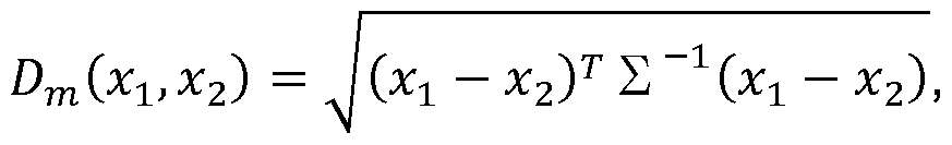
where ∑ is the covariance matrix of the multivariate Gaussian probability density function. [18] The quantile threshold may be fixed once for all and stored as a constant in the system implementing the method. Preferably, however, the quantile threshold is a monotonously varying function of the variance of the speed variation (or the variance of the longitudinal acceleration), such that a lower proportion of events are considered abnormal in case of low acceleration variance and a higher proportion of events are considered abnormal in case of high acceleration variance. The quantile threshold as a function of the acceleration variance may e.g. be stored in the system in the form of a lookup table. As will be appreciated, such a dynamic quantile threshold also contributes to the mitigation of effects caused by the deterioration of the diversity of the modelled population of feature vectors. When the driver drives in a very aggressive way (reflected by high statistical variance of the longitudinal acceleration), the quantile threshold applied in the computation of the severity score is increased. More anomalous events are thus detected. With the above formula for calculating the severity indicator, more events will obtain a non-zero severity score and the scores reaches will tend to be higher when the acceleration variance is high. In the opposite situation of monotonous driving (reflected by low statistical acceleration variance),
possible accompanied by the narrowing of the multivariate Gaussian distribution, the quantile threshold applied in the computation of the severity score is decreased. The system thus tends to detect less anomalous events. It should be noted that the variance of longitudinal acceleration might be expressed in a discrete-time system as the variance of the speed variation, i.e. the variance of the speed difference between subsequent time steps.
[19] The first vector component of the feature vector may be speed variation and the second vector component may be bearing variation.
[20] According to a more preferred embodiment of the method, the first vector component is the product of speed variation Δν (longitudinal acceleration) and standard deviation of the modulus of jerk, noted o(j), and the second vector component is the product of bearing variation, noted Ab, and standard deviation of the modulus of jerk. In the context of the present document, "jerk" designates the derivative of the acceleration vector with respect to time. The speed variation and the bearing variation are preferably obtained through a GNSS receiver, while the jerk is preferably obtained by an accelerometer. The features (components of the feature vectors) will thus indicate whether there is constructive consensus between the GNSS data and the accelerometer data.
[21 ] According to an alternative embodiment, the first vector component is the product of speed, speed variation and standard deviation of the norm of the jerk vector and the second vector component is the product of speed, bearing variation and standard deviation of the modulus of jerk. Compared to the above-mentioned option, the products in this embodiment have the additional advantage of mitigating heteroscedasticity (i.e. heterogeneous variance) of the features. The Av o(j) term tends to exhibit lower variance at higher speeds than at lower speeds.
[22] The one or more sensors may be operated at the same or different acquisition rates. In case of different acquisition rates, the sets of motion observations are preferably produced at the feature vector refresh rate by data fusion involving sampling and/or interpolation and/or extrapolation and/or filtering and/or averaging. Each sensor typically produces its data at a particular rate. Acceleration sensors may e.g. work at several tens of Hz or higher frequencies, whereas the data rate of GNSS navigators is typically of the order of 1 Hz. At the fusion layer, depending on the desired refresh rate of the feature vectors, raw data arriving with lower rates may be upsampled while data
arriving with higher rates may be downsampled. The fusion layer may also be used to process the data and to produce statistical data such as, e.g., variances, standard deviations, averages, etc. and other derived data such as, e.g., derivatives, ratios, products, moduluses, etc. Both the raw data and the data produced by the fusion layer are considered herein as motion observations.
[23] According to a preferred embodiment of the method, the motion observations are captured with at least one of a GNSS receiver (also: GNSS navigator), an accelerometer and a magnetometer.
[24] Preferably, the method according to the first aspect of the invention comprises the wireless transmission of at least the integrated riskiness indicator, e.g. to a data center. That transmission may be scheduled to recur at fixed times, after fixed time intervals, after each trip or after a defined distance travelled. The recipient of the data may e.g. be an insurance company, a fleet manager, a car leasing company, a social network, a public institution, etc. Further to the integrated riskiness indicator, the transmitted data preferably include an identifier of the driver, the distance travelled during the integration period. One advantage of the method is that the amount of transmitted data may be kept very small. Furthermore, detailed information about specific driving events, the driver's location, the travel history, etc. need not be transmitted, as it would be the case if the riskiness indicator had to be calculated on a remote site. The driver's privacy may thus be protected to a large extent. Nevertheless, more detailed information could be included into the transmitted data, such as, e.g., the number of risky events (events with a non-zero severity score), the locations of these events, their frequency, etc. A detailed log of the trips of the vehicle could also be achieved by the system and transmitted to the data center. Appropriate measures may be taken to guarantee the driver's privacy. These may include secure transmission and storage of the data. The storage of the data may furthermore be achieved such that access restrictions can be enforced. Preferably, any detailed logs are stored in an anonymized manner.
[25] A second aspect of the invention relates to a mobile electronic device application (an "app") comprising instructions, which, when executed by a processor of a mobile electronic device, such as, e.g. a smartphone, a tablet, a phablet, a notebook or the like, cause the mobile electronic device to carry out the method as described herein.
[26] A third aspect of the invention relates to a vehicular motion monitoring method comprising:
a) capturing motion observations on-board a vehicle with one or more sensors; b) mapping sets of motion observations onto a respective feature vector in a feature space, each set of motion observations corresponding to a driving event and comprising a speed observation, which the feature vector is associated to through the mapping;
c) classifying the driving event based upon, at least, the feature vector and a probability density function modelling a population of collected feature vectors, the classifying preferably comprising outputting and/or forwarding the identified event class;
d) updating (and at least temporarily memorizing in a computer data storage) determinative parameters of the probability density function, the updating comprising:
entering the feature vector into a buffer memory so as to update the population of collected feature vectors and recalculating the determinative parameters, the buffer memory comprising a plurality of cyclic buffers, each cyclic buffer containing a sub-population of collected feature vectors corresponding to a specific speed range, and wherein entering the feature vector into the buffer memory comprises entering the feature vector into the cyclic buffer that corresponds to the speed range, which the speed observation of the feature vector belongs to.
[27] It shall be noted that the vehicular motion monitoring method according to the third aspect of the invention does not necessarily comprise all limitations of the method according to the first aspect of the invention and could be claimed separately, e.g. via a divisional or continuation application. In particular, the vehicular motion monitoring method according to the third aspect of the invention may comprise one or more, but preferably not all, of the following characteristics I to V:
I. the feature space is two-dimensional;
II. the feature vector has a first vector component representative of a longitudinal motion characteristic and a second vector component representative of a lateral motion characteristic;
III. the probability density function is a multivariate Gaussian probability density function;
IV. a riskiness indicator (a numerical score representing riskiness) is assigned to each feature vector (or to each driving event), the calculation of the riskiness indicator being based upon an event severity indicator (or severity score) indicative of how anomalous each feature vector is in comparison to the modelled population and upon a position of the feature vector relative to one or more previous and/or subsequent feature vectors;
V. the riskiness indicator is integrated over time (e.g. in a memory space allocated to that indicator) so that a risk assessment of the driving style of the driver of the vehicle is obtained.
[28] Particularly preferred combinations of characteristics I to V are: o I but not any one of II to V; o I and II but not any one of III to V; o III but not any one of I, II, IV and V; o III and at least one of I and II, but not at least one of IV and V; o IV but not any one of I, II, III and V; o IV and V but not at least one of I to III.
[29] Any optional feature disclosed hereinbefore in the context of the description of the method according to the first aspect of the invention may equally be applied in the method according to the third aspect of the invention.
[30] The term "determinative parameters" of a probability density function designates any set of parameters that completely defines the probability density function. [31 ] As explained above in the context of the first aspect of the invention already, entering a feature vector into the buffer memory comprises entering the feature vector into the cyclic buffer that corresponds to the speed range, which the speed observation associated with the feature vector belongs to. Dynamically updating the population of collected feature vectors always bears the risk that the updated population is less representative of "ordinary" driving behaviour than the previous population. Prolonged
monotonous driving on motorways, for instance, may lead to a less diverse (and in that sense impoverished) population of feature vectors. In consequence, classifying driving events following monotonous driving periods may lead to different results than after diversified driving. More or less complex updating criteria may thus have to be put into place to ascertain that the modelled population does not deteriorate too much. The plurality of cyclic buffers helps to mitigate the deterioration problem. Each time a feature vector is added to the population, it is in fact added to the cyclic buffer corresponding to the same speed category (speed range). This means that each newly arrived feature vector does not automatically replace the oldest feature vector of the entire population but replaces the oldest feature vector within the same speed category. With those measures, monotonous driving still leads to some loss of population diversity but this loss will typically be limited to one or two cyclic buffers, i.e. one or two speed categories. The remaining cyclic buffers remain essentially unaffected. As all the sub-populations make up the modelled population, the overall impact of diversity deterioration on the classification can be kept on a low level. The cyclic buffers may all be of the same size (i.e. contain the same number of collected feature vectors) or of different sizes. The latter option may be used to give more or less weight to specific speed categories. If this option should be implemented, care should be taken not to attribute too much relative weight to speed categories in which monotonous driving is particularly likely to occur.
[32] In the vehicular motion monitoring method according to the third aspect of the invention, the step of classifying the driving event may comprise assigning the driving event to one of at least two riskiness categories. A crude classification would consist in classifying each driving event either as "safe" (or "unrisky" or the like) or "risky" (or "dangerous" or the like). A more subtle classification may be achieved by using one or more intermediate categories between those extremes. Classification could also rely on a severity score or a riskiness score as described above.
[33] Classification of a driving event may additionally be based upon data not necessarily (directly) related to vehicular motion, such as e.g. geographical position of the vehicle, time of day, weather conditions (temperature, precipitation, etc.), traffic conditions, speed limits and other traffic rules, etc. These additional data are preferably included into the feature vector. According to an advantageous embodiment of a method according to the third aspect of the invention, these additional data are used
to take environmental conditions into account for classification of the driving events. The geographical position may e.g. be used to assign a higher severity score or riskiness score if a driving event occurred in a zone known to be particularly dangerous (based e.g. on accident statistics). Time of day (or daylight information), weather and traffic information could be used in a similar manner: somewhat risky driving events could be classified as even more risky if they occur at night time, in bad weather or in dense traffic. Cumulation of adverse environmental conditions preferably leads to a still higher riskiness class or score. Driving event classification could further be made dependent on the respect of traffic rules. If, for instance, it is detected that the vehicle is exceeding the speed limit an otherwise "unrisky" driving event could be classified as a (more) risky one.
[34] The vehicular motion monitoring method according to the third aspect of the invention is preferably implemented on a mobile (electronic) device, such as, e.g. a smartphone, a tablet, a phablet, a notebook or the like. Accordingly, a fourth aspect of the invention relates to a mobile electronic device application comprising instructions, which, when executed by a processor of a mobile electronic device, cause the mobile electronic device to carry out the method according to the third aspect of the invention.
[35] If the vehicle is equipped with one or more assistant systems such as, e.g., a drowsiness detector, a lane departure warning assistant, a distance monitoring system (for monitoring the distance to a vehicle ahead), a traffic sign recognition system, a rain sensor, etc., a data link to between the mobile device and the car may be beneficial. Accordingly, the app is preferably configured to wirelessly connect the mobile device to the vehicle's onboard communication network or at least to attempt to establish such a connection, and in case of successful connection, listening to the messages of any assistant system installed on the vehicle.
Brief Description of the Drawings
[36] By way of example, preferred, non-limiting embodiments of the invention will now be described in detail with reference to the accompanying drawings, in which:
Fig. 1 : is a schematic illustration of a mobile electronic device for running an app carrying out the method according to the first aspect of the invention;
Fig. 2: is a schematic flow chart of a preferred embodiment of the method;
Fig. 3: is an illustration of the conceptual structure of a buffer memory with several cyclic buffers storing each a sub-population of the collected feature vectors;
Fig. 4: is a chart illustrating how the quantile threshold may be varied as a function of acceleration variance; Fig. 5: is a chart illustrating severity scores obtained during test drives under controlled conditions;
Fig. 6: is a diagram of the evolution of the feature vectors during a slalom drive;
Fig. 7: is an illustration of the classification of driving events using normalized feature vectors; Fig. 8: is a chart which compares two choices of features;
Fig. 9: is a schematic flow chart of a preferred embodiment of a method according to the third aspect of the invention.
Detailed Description of a Preferred Embodiment of the Invention
[37] A multivariate normal (MVN) model is used to detect risky driving maneuvers and profile drivers. To the inventors' best knowledge, this is the first time an MVN approach is considered for driver profiling. While previous driver profiling methods considered high sensor outputs or pre-established patterns in order to declare a risky driving maneuver or event, given the heterogeneity of both mobile devices and vehicles, the inventors believe that a profiling system needs to adapt its parameters to each individual context. Traditional fixed threshold or supervised machine learning techniques (e.g., neural networks or naive Bayes) may be suitable for designing such a driver profiling mechanism but require previous knowledge on the training samples, indicating the expected values of the input variables at the exact time a risky maneuver is performed. Then, the generation of such a training data set for risky driving maneuvers for different devices and vehicles becomes unfeasible in practice. Moreover, it cannot be a prerequisite of the application that the final users manually label risky driving maneuvers in a training phase.
[38] As it turned out during the development of the invention, an MVN-based anomaly detection fits well with the problem to model. First, it provides a high flexibility by dynamically adapting to different driving conditions with recurring updates of its determinative parameters. Also, given that it does not require any preliminary
knowledge on the driving events it has to detect, it can be applied to any type of vehicle and mobile device.
[39] In general, the MVN model has many advantages over other approaches for anomaly detection: o There is no need to establish rule sets or thresholds to detect risky maneuvers.
The probability of an observation enables the assessment of driver behaviour in a continuous or quasi-continuous fashion rather than binary classification (i.e., discerning merely between risky and non-risky driving events). o The model can be estimated efficiently on a mobile phone or any other mobile electronic device and can be continuously retrained to improve the parameter estimates. The memory footprint may be held essentially constant in time, since the population of feature vectors may be stored in cyclic buffers. Also the computation time for the model fitting is bounded and the complexity does not increase over time. o The model can represent covariance among features (which is expected to be seen in vehicular dynamics).
[40] Fig. 1 schematically illustrates a mobile electronic device 10, e.g. a smart phone, equipped with several sensors, in particular, a GNSS navigator 12, a three-axis acceleration sensor 14 and a three-axis magnetometer 16. The sensors are connected to the processor 18 of the mobile device 10. A communications module 20 allows the mobile device to establish and accept wireless connections. The mobile electronic device 10 may be used to execute an app that uses the data captured by the sensors 12, 14, and 16 to monitor vehicular motion and to assess the riskiness of the driving style in accordance with the present invention. [41 ] A flowchart illustrating a preferred embodiment of a method according to the invention is provided in Fig. 2. As illustrated, the mobile device collects input variables (motion observations) using the available sensors 12, 14 and 16. The motion observations are then transformed into respective elements (feature vectors) in a two- dimensional feature space that aims at representing the longitudinal and lateral axes of movement of the vehicle. These feature vectors are stored in a training buffer. When the app is executed for the first time, the feature vectors are accumulated in the training buffer until a critical size is reached and the first MVN model can be computed using
e.g. the maximum likelihood estimator (MLE). At the time the first MVN model has been computed, the app becomes fully operational and begins to determine the severity of driving events and to compute the riskiness indicator as detailed hereinafter. Newly arriving feature vectors continue to be collected in the training buffer and the MVN model adjusted in consequence, e.g. by using the above-mentioned MLE.
[42] The GNSS navigator 12 produces its data (position vector, velocity vector and time) typically at a rate of the order of 1 Hz, whereas the accelerometer 14 issues acceleration vectors at a significantly higher rate (typically 20 Hz to 50 Hz in smartphones) and the acquisition rate of the magnetometer lies typically in the range from 20 to 200 Hz. The raw data provided by the different sensors at the different rates are combined and synchronised by the processor. Conceptually, this corresponds to a fusion layer 22, as shown in Fig. 2. Data acquired from faster sensors are buffered between two consecutive inputs from the slowest sensor (in our example the navigator). Motion observations at the desired refresh rate (e.g. 10 Hz) are obtained by upsampling and downsampling data acquired at lower and higher rates, respectively. The fusion layer also makes available derived data. For the following description of a preferred example of the method, it will be assumed that the motion observations made available at the desired refresh rate are: o(j) the standard deviation of the norm of the jerk vector. The jerk vector is computed as the derivative with respect to time of the acceleration vector output by the accelerometer 14. v the speed calculated based upon data from the navigator 12 (with interpolation)
Δν the speed variation from one time step to the next σ(Δν) the standard deviation of Δν
Ab the bearing variation from one time step to the next, calculated based upon data from the navigator 12 (with interpolation) and from the magnetometer 16.
[43] Each set of motion observations o = {o(j), v, Δν, σ(Δν), Ab} is then mapped onto an element (feature vector), x, of a two-dimensional feature space, X (x ε X). Each feature vector has a first vector component (feature) representative of a longitudinal motion characteristic and a second vector component representative of a lateral motion characteristic, with the following properties: i) extreme values of the
features represent risky or abnormal driving maneuvers, ii) feature distribution can be approximated by a Gaussian distribution. The mapping step is illustrated in Fig. 2 by step 24.
[44] In the present example, the first feature is selected as the product of Δν and o(j) and the second feature is selected as the product of Ab and o(j): x = (x1, x2) = (Δν■ a(_j), Ab■ σ(/)) -
[45] Other possibilities would be (,x1, x2) = (Av, Ab) or (x1, x2) = (Δν■ σ( ) - v, Ab · σ( ) ■ v) but these are not discussed further hereinafter.
[46] The MVN model can be defined by a multivariate Gaussian probability density function:

where d denotes the dimension of the feature space X, μ the center of the distribution (mean vector) and∑ the so-called covariance matrix. The determinative parameters μ and∑ are obtained through a training process (steps 26 and 28) in Fig. 2. [47] The training process is executed in parallel with the event assessment process, which includes computing the severity of events (step 30), computing the riskiness indicator (step 32) and integrating the riskiness indicator over time (step 34). The training process is preferably continuous but could also be intermittent. In a continuous training process, each feature vector obtained in the mapping step is fed to a buffer memory (step 26), in which a population of previously collected feature vectors is maintained. A multivariate Gaussian probability density function is fitted to the population using the MLE, which yields the determinative parameters μ and∑.
[48] A preferred example of how the feature vector population can be maintained is illustrated in Fig. 3. The buffer memory comprises a plurality of cyclic buffers (represented as columns in Fig. 3). Each cyclic buffer contains a sub-population of the collected feature vectors corresponding to a specific speed range. In the illustrated example, there are 7 cyclic buffers, each corresponding to a speed range of 30 km/h. It is assumed that the entire speed range of the vehicle is covered by the buffers, otherwise the uppermost speed range may be open-ended. When a new feature vector is available, it is entered into the cyclic buffer that corresponds to the speed range of the speed observation v of the set of motion observations underlying the feature vector.
If a cyclic buffer is completely filled up, the newly added feature vector replaces or overwrites the oldest feature vector of that cyclic buffer. In Fig. 3 all cyclic buffers are of the same size, but that may be implemented differently. Prolonged monotonous driving may lead to an overly homogeneous population of feature vectors in one or two cyclic buffers. However, situations, in which the entire population of feature vectors (which is used for the computation of μ and∑) would be degraded to an extent that it produces only meaningless results, are extremely unlikely due to the "isolation" of the cyclic buffers from each other. Monotonous driving still leads to some loss of population diversity on the scale of the entire population but the overall impact thereof on the severity score and on the riskiness score can be kept on a low level.
[49] For every given set of motion observations o and its corresponding feature vector x, a metric for the severity (or risk factor) is computed. To this end, a cut-off quantile threshold, Qiim, is proposed that marks the quantile limit between common observations and those that are considered to be anomalous. Qiim defines a cut-off probability value, piim, which can be used to classify the samples. Let pnm be the value of the model-dependent inverse cumulative distribution function (CDF) of Qiim, and Q(x) the (approximate) quantile of the feature transform x of observation o, then the severity indicator may be expressed as:

[50] The severity indicator s defines a normalised metric of how anomalous a set of motion observations o or the corresponding feature vector x is. Qiim is typically chosen in the range from 10"5 to 10"2 (1 %). Lower values of Qiim will result in in fewer feature vectors being considered anomalous (i.e. being assigned a severity score different from 0). Qiim may be a constant in the application but a way to dynamically vary Qnm will be presented further down in the text.
[51 ] The above expression for s(x) may be rewritten in the following form:
 where Dlim = -2 log(l - Qlim) and Dm designates the Mahalanobis distance depending on the parameter∑.
[52] A dynamic quantile threshold Qiim is considered advantageous. When the user drives in an aggressive way, which is reflected by a high statistical variance of Δν (i.e. of the acceleration), the quantile threshold Qiim is increased, such that more anomalous events are detected. Lower variance of Δν will translate into a lower Qnm, such that less anomalous events are detected. Fig. 4 illustrates one possible relationship between σ(Δν) and 1 -Qum. A low quantile threshold of 10"5 is assigned to feature vectors for a σ(Δν) close to zero. Qiim then increases like a quadratic function up to 0.1 until σ(Δν) = 5.5 m/s2. For σ(Δν) > 5.5 m/s2 Qiim remains 0.1 . Qiim as a function of σ(Δν) is preferably stored as a lookup table in the app. For the computation of s(x), the applicable value of Qiim may thus be retrieved from that table.
where Dlim = -2 log(l - Qlim) and Dm designates the Mahalanobis distance depending on the parameter∑.
[52] A dynamic quantile threshold Qiim is considered advantageous. When the user drives in an aggressive way, which is reflected by a high statistical variance of Δν (i.e. of the acceleration), the quantile threshold Qiim is increased, such that more anomalous events are detected. Lower variance of Δν will translate into a lower Qnm, such that less anomalous events are detected. Fig. 4 illustrates one possible relationship between σ(Δν) and 1 -Qum. A low quantile threshold of 10"5 is assigned to feature vectors for a σ(Δν) close to zero. Qiim then increases like a quadratic function up to 0.1 until σ(Δν) = 5.5 m/s2. For σ(Δν) > 5.5 m/s2 Qiim remains 0.1 . Qiim as a function of σ(Δν) is preferably stored as a lookup table in the app. For the computation of s(x), the applicable value of Qiim may thus be retrieved from that table.
[53] Fig. 5 illustrates severity scores obtained during test drives under controlled conditions. Phases of normal driving were alternated with phases of exceptionally stark accelerations and decelerations (shaded areas) both in longitudinal and lateral directions. The speed is shown in the top graph as a reference. The bottom graph illustrates the severity score as a function of time. It can be seen that the anomalous driving events could be reliably detected.
[54] The severity indicator (or score) indicates how anomalous an event is. A riskiness indicator is computed for each feature vector at step 32. In order to analyse riskiness, the evolution of the feature vectors over time is taken into account. [55] Using the severity metric s(x) defined above as well as the Mahalanobis distance Dm, a risk function is defined by:

where the indexes i and i-1 denote the current feature vector and the previous one, respectively, where haversin(a) = (1 - cos(a))/2 and where a designates the Mahalanobis angle between x, and X subtended at μ:

[56] Fig. 6 illustrates the evolution of the feature vectors over time during driving a slalom. The arrows show the transitions between consecutive feature vectors. The boundary separating ordinary from anomalous feature vectors is shown as a white line. In the interior area the severity score and the riskiness scores of the feature vectors
are both 0. The grey disks surrounding each feature vector have radii proportional to the corresponding riskiness indicator R(x). The slalom trace shows variance in both dimensions of the feature space, as it can be observed in the diagonal transition lines between subsequent observations This is because the driver needs to constantly adapt speed (i.e., accelerate and brake) in order to pass between two obstacles.
[57] The riskiness indicator is accumulated (integrated) over time (step 34 in Fig. 2), e.g. during a trip. The integrated riskiness indicator∑£ Λ (Λ:£) then serves as a basis for driver scoring. The integrated riskiness indicator is finally transmitted (step 36 in Fig. 2) to a data center, together with an identifier of the driver (and/or of the mobile device on which the app is executed) and further data, such as, e.g. the time and/or the distance over which was integrated.
[58] The two-dimensional feature space with features vectors (x1, x2) = (Δν a(j),Ab ■ σ( )) or (x1, x2) = (Av, Ab) or (x1, x2) = (Δν■ a(j) - v, Ab - a(j)■ v) presented hereinabove distinguishes lateral and longitudinal motions. This may be used to identify different types of events (steering left, acceleration, steering right and braking). The feature vector components may be scaled by subtracting the mean of each feature and dividing it by its standard deviation:

Using the proposed scaling, the effects of different ranges for the different features is compensated. As illustrated in Fig. 7, the scaled feature space may be divided into four
90°-sectors representing acceleration events (^ < φ < y), braking events (y < φ < y) and steering events (y < φ < y) and (y i. e.1^ < φ < ^). Note that in Fig. 7, the roles of zi and∑2 are inverted.
[59] For the purpose of event classification, the polar coordinate φ of the scaled or normalized feature vectors z may be averaged over several (e.g. 4) consecutive events. The event category may be computed for every feature vector. Preferably, however, the event category is only calculated for anomalous events (having a nonzero severity score s).
[60] The app may be configured so as not to log the individual events. In this case, the integrated riskiness indicator ∑i R (Xi) will be transmitted without detailed
information as to how the integrated score was reached. As a first alternative, the app could be configured to log and transmit all events but that implies that a lot of data have to be processed, which are of little value. As a second alternative, the app may be configured to log the anomalous events. The app could e.g. be configured to store and transmit the category of such events, their position and time, the severity score and the riskiness indicator. In that way, the relevant data can be transmitted to the data center while impacting the communication networks significantly less.
[61 ] As briefly stated hereinabove, the feature vectors with (x1, x2) = (Av■ a(j)■ v,Ab■ a(j)■ v) may be used to mitigate heteroscedasticity. For all automotive vehicles, maximum acceleration decreases with increasing speed. It follows that the statistical variance of Δν is lower at high speeds than at lower speeds. By multiplying Av■ a(j) and Ab■ a(j) with the speed v, that effect is compensated to some extent. This is illustrated in Fig. 8, which shows a comparison of the features Av■ a(j) and Av■ a(j)■ v recorded over 30 s during which a car was accelerated from 20 km/h to about 150 km/h with the accelerator pedal fully pushed down.
[62] A flowchart illustrating a further preferred embodiment of a method according to an aspect of the invention is provided in Fig. 9. As illustrated, the mobile device collects input variables (motion observations) using the sensors 1 12, 1 14 and 1 16. The motion observations are then transformed into respective elements (feature vectors) in a feature space that aims at representing characteristics of the movement of the vehicle. These feature vectors are stored in a training buffer. When the app is executed for the first time, the feature vectors are accumulated in the training buffer until a critical size is reached and the determinative parameters of a probability density function modelling the population can be computed using an appropriate estimator. At the time the first parameter set has been computed, the app becomes fully operational and begins to classify driving events as detailed hereinafter. Newly arriving feature vectors continue to be collected in the training buffer and the determinative parameters are adjusted in consequence.
[63] When the raw data are provided by the sensors 1 12, 1 14, 1 16 at different rates, they are combined and synchronised by the processor. Conceptually, this corresponds to a fusion layer 122, as shown in Fig. 9. Data acquired from faster sensors are buffered between two consecutive inputs from the slowest sensor. Motion observations at the desired refresh rate are obtained by upsampling and downsampling data
acquired at lower and higher rates, respectively. The fusion layer 122 also makes available derived data.
[64] Each set of motion observations corresponding to a driving event is mapped onto an element (feature vector), x, of a feature space, X (x ε X). Each feature vector has one or more components corresponding to motion characteristics with the following properties: i) extreme values of the features represent risky or abnormal driving maneuvers, ii) feature distribution can be approximated by a parameterizable probability density function. The mapping step is illustrated in Fig. 9 by step 124.
[65] The determinative parameters of the probability density function are obtained through a training process (steps 126 and 128 in Fig. 9).
[66] The training process is executed in parallel with driving event classification (step 130). The training process is preferably continuous but could also be intermittent. In a continuous training process, each feature vector obtained in the mapping step is fed to a buffer memory (step 126), in which a population of previously collected feature vectors is maintained. A probability density function (e.g. a multivariate Gaussian probability density function) is fitted to the population using an appropriate estimator, which yields the determinative parameters of the probability density function. The feature vector population can be maintained as previously described with respect to Fig. 3. [67] The classification results are transmitted (step 136 in Fig. 9) to a data center, together with an identifier of the driver (and/or of the mobile device on which the app is executed) and further data, such as, e.g. the time, the distance covered and/or the geographic position.
[68] While specific embodiments have been described herein in detail, those skilled in the art will appreciate that various modifications and alternatives to those details could be developed in light of the overall teachings of the disclosure. Accordingly, the particular arrangements disclosed are meant to be illustrative only and not limiting as to the scope of the invention, which is to be given the full breadth of the appended claims and any and all equivalents thereof.
Claims
A vehicular motion monitoring method comprising
a) capturing motion observations on-board a vehicle with one or more sensors; b) mapping sets of motion observations onto a respective feature vector in an at least two-dimensional feature space, each feature vector having a first vector component representative of a longitudinal motion characteristic and a second vector component representative of a lateral motion characteristic; c) updating determinative parameters of a multivariate Gaussian probability density function modelling a population of collected feature vectors;
d) assigning a riskiness indicator to each feature vector, calculation of the riskiness indicator being based upon an event severity indicator indicative of how anomalous each feature vector is in comparison to the modelled population and upon a position of the feature vector relative to one or more previous and/or subsequent feature vectors;
e) integrating the riskiness indicator over time so as to obtain a risk assessment of driving style of the driver of the vehicle.
The vehicular motion assessment method as claimed in claim 1 , wherein updating the determinative parameters of the multivariate Gaussian probability density function comprises entering each feature vector into a buffer memory so as to update the population of collected feature vectors and recalculating said determinative parameters.
The vehicular motion assessment method as claimed in claim 2, wherein each set of motion observations comprises a speed observation, to which said feature vector is associated through said mapping, wherein said buffer memory comprises a plurality of cyclic buffers, each cyclic buffer containing a sub- population of collected feature vectors corresponding to a specific speed range, and wherein entering each feature vector into the buffer memory comprises entering said feature vector into the cyclic buffer that corresponds to the speed range, which the speed observation of said feature vector belongs to.
The vehicular motion assessment method as claimed in any one of claims 1 to 3, wherein said severity indicator is calculated for each feature vector based on the determinative parameters of the multivariate Gaussian probability density
function and a quantile threshold representative of a proportion of events considered abnormal.
5. The vehicular motion assessment method as claimed in claim 4, comprising adjusting said quantile threshold monotonously depending on acceleration variance such that a lower proportion of events are considered abnormal in case of low acceleration variance and a higher proportion of events are considered abnormal in case of high acceleration variance.
6. The vehicular motion assessment method as claimed in any one of claims 1 to 5, wherein said first vector component is the product of speed variation and standard deviation of the modulus of jerk and wherein the second vector component is the product of bearing variation and standard deviation of the modulus of jerk.
7. The vehicular motion assessment method as claimed in any one of claims 1 to 5, wherein said first vector component is the product of speed, speed variation and standard deviation of the modulus of jerk and wherein the second vector component is the product of speed, bearing variation and standard deviation of the modulus of jerk.
8. The vehicular motion assessment method as claimed in any one of claims 1 to 7, wherein said one or more sensors are operated at different acquisition rates and wherein said sets of motion observations are produced by data fusion involving sampling and/or interpolation and/or extrapolation and/or filtering and/or averaging.
9. The vehicular motion assessment method as claimed in any one of claims 1 to 8, wherein said motion observations are captured with at least one of a GNSS receiver, an accelerometer and a magnetometer.
10. The vehicular motion assessment method as claimed in any one of claims 1 to 8, comprising wireless transmission of at least the integrated riskiness indicator.
1 1 . Mobile electronic device application comprising instructions, which, when executed by a processor of a mobile electronic device, such as, e.g. a smartphone, a tablet, a phablet, a notebook or the like, cause the mobile electronic device to carry out the method as claimed in any one of claims 1 to 10.
Applications Claiming Priority (2)
| Application Number | Priority Date | Filing Date | Title |
|---|---|---|---|
| LU92628 | 2015-01-02 | ||
| LU92628A LU92628B1 (en) | 2015-01-02 | 2015-01-02 | Vehicular motion monitoring method |
Publications (1)
| Publication Number | Publication Date |
|---|---|
| WO2016107876A1 true WO2016107876A1 (en) | 2016-07-07 |
Family
ID=52355126
Family Applications (1)
| Application Number | Title | Priority Date | Filing Date |
|---|---|---|---|
| PCT/EP2015/081361 WO2016107876A1 (en) | 2015-01-02 | 2015-12-29 | Vehicular motion monitoring method |
Country Status (2)
| Country | Link |
|---|---|
| LU (1) | LU92628B1 (en) |
| WO (1) | WO2016107876A1 (en) |
Cited By (6)
| Publication number | Priority date | Publication date | Assignee | Title |
|---|---|---|---|---|
| IT201700061227A1 (en) * | 2017-06-05 | 2018-12-05 | Francesco Odori | SYSTEM AND METHOD FOR MONITORING AND REMOTE CONTROL OF THE VEHICLE OPERATING PARAMETERS |
| FR3070332A1 (en) * | 2017-08-31 | 2019-03-01 | Valeo Vision | LIGHTING DEVICE FOR A LUMINOUS BEAM WITH A DAMED CENTRAL ZONE |
| WO2019197345A1 (en) | 2018-04-09 | 2019-10-17 | Motion-S | Vehicular motion assessment method |
| CN111985850A (en) * | 2020-09-04 | 2020-11-24 | 吉林大学 | Driving risk control method, driving risk control device and computer storage medium |
| CN113635915A (en) * | 2021-08-24 | 2021-11-12 | 中国人民解放军陆军装甲兵学院 | Vehicle driving early warning method and device, electronic equipment and storage medium |
| CN114222689A (en) * | 2019-08-23 | 2022-03-22 | 沃尔沃卡车集团 | Method for quantifying extreme traffic behavior |
Citations (3)
| Publication number | Priority date | Publication date | Assignee | Title |
|---|---|---|---|---|
| US20090040054A1 (en) * | 2007-04-11 | 2009-02-12 | Nec Laboratories America, Inc. | Real-time driving danger level prediction |
| DE102009009975A1 (en) * | 2008-09-24 | 2010-04-01 | Audi Ag | Driver alertness determining method for use during motorway journey in car, involves statistically evaluating measured values to determine statistical value, and determining alertness value under consideration of statistical value |
| US20110029184A1 (en) * | 2009-07-31 | 2011-02-03 | Systems and Advances Technologies Engineering S.r.I. (S.A.T.E.) | Road Vehicle Drive Behaviour Analysis Method |
-
2015
- 2015-01-02 LU LU92628A patent/LU92628B1/en active
- 2015-12-29 WO PCT/EP2015/081361 patent/WO2016107876A1/en active Application Filing
Patent Citations (3)
| Publication number | Priority date | Publication date | Assignee | Title |
|---|---|---|---|---|
| US20090040054A1 (en) * | 2007-04-11 | 2009-02-12 | Nec Laboratories America, Inc. | Real-time driving danger level prediction |
| DE102009009975A1 (en) * | 2008-09-24 | 2010-04-01 | Audi Ag | Driver alertness determining method for use during motorway journey in car, involves statistically evaluating measured values to determine statistical value, and determining alertness value under consideration of statistical value |
| US20110029184A1 (en) * | 2009-07-31 | 2011-02-03 | Systems and Advances Technologies Engineering S.r.I. (S.A.T.E.) | Road Vehicle Drive Behaviour Analysis Method |
Non-Patent Citations (1)
| Title |
|---|
| IM SEONGSU ET AL: "Driver distraction detection by in-vehicle signal processing", 2014 IEEE SYMPOSIUM ON COMPUTATIONAL INTELLIGENCE IN VEHICLES AND TRANSPORTATION SYSTEMS (CIVTS), IEEE, 9 December 2014 (2014-12-09), pages 64 - 68, XP032720672, DOI: 10.1109/CIVTS.2014.7009479 * |
Cited By (9)
| Publication number | Priority date | Publication date | Assignee | Title |
|---|---|---|---|---|
| IT201700061227A1 (en) * | 2017-06-05 | 2018-12-05 | Francesco Odori | SYSTEM AND METHOD FOR MONITORING AND REMOTE CONTROL OF THE VEHICLE OPERATING PARAMETERS |
| FR3070332A1 (en) * | 2017-08-31 | 2019-03-01 | Valeo Vision | LIGHTING DEVICE FOR A LUMINOUS BEAM WITH A DAMED CENTRAL ZONE |
| WO2019042702A1 (en) * | 2017-08-31 | 2019-03-07 | Valeo Vision | Lighting device for a light beam with a dark central area |
| WO2019197345A1 (en) | 2018-04-09 | 2019-10-17 | Motion-S | Vehicular motion assessment method |
| CN114222689A (en) * | 2019-08-23 | 2022-03-22 | 沃尔沃卡车集团 | Method for quantifying extreme traffic behavior |
| CN111985850A (en) * | 2020-09-04 | 2020-11-24 | 吉林大学 | Driving risk control method, driving risk control device and computer storage medium |
| CN111985850B (en) * | 2020-09-04 | 2022-04-22 | 吉林大学 | Driving risk control method, driving risk control device and computer storage medium |
| CN113635915A (en) * | 2021-08-24 | 2021-11-12 | 中国人民解放军陆军装甲兵学院 | Vehicle driving early warning method and device, electronic equipment and storage medium |
| CN113635915B (en) * | 2021-08-24 | 2023-01-06 | 中国人民解放军陆军装甲兵学院 | Vehicle driving early warning method and device, electronic equipment and storage medium |
Also Published As
| Publication number | Publication date |
|---|---|
| LU92628B1 (en) | 2016-07-04 |
Similar Documents
| Publication | Publication Date | Title |
|---|---|---|
| US11836802B2 (en) | Vehicle operation analytics, feedback, and enhancement | |
| US11891071B2 (en) | Vehicle to vehicle telematics | |
| US11295391B1 (en) | Reward system related to a vehicle-to-vehicle communication system | |
| US11551309B1 (en) | Reward system related to a vehicle-to-vehicle communication system | |
| US11727495B1 (en) | Collision risk-based engagement and disengagement of autonomous control of a vehicle | |
| US20220244063A1 (en) | Data processing system communicating with a map data processing system to determine or alter a navigation path based on one or more road segments | |
| US10414407B1 (en) | Driving analysis using vehicle-to-vehicle communication | |
| US10332390B1 (en) | Driving event data analysis | |
| WO2016107876A1 (en) | Vehicular motion monitoring method | |
| US10664918B1 (en) | Insurance system related to a vehicle-to-vehicle communication system | |
| JP2023168361A (en) | Information processing system, information processing method, and program | |
| US20170372431A1 (en) | Autonomous or partially autonomous motor vehicles with automated risk-controlled systems and corresponding method thereof | |
| CN110807930B (en) | Dangerous vehicle early warning method and device | |
| Zeeman et al. | Combining speed and acceleration to detect reckless driving in the informal public transport industry | |
| JP2020521978A (en) | Systems and methods for determining safe routes | |
| US20240005411A1 (en) | Systems and methods for modeling telematics, positioning, and environmental data | |
| CN110827152A (en) | Insurance evaluation method, system and server | |
| US20240013310A1 (en) | Fully integrated and embedded measuring system directed to a score-indexing parameter essentially based on directly measured connected motor vehicle sensory data and method thereof | |
| CN115472040B (en) | Personalized anti-collision early warning method for networked vehicle based on collision probability field | |
| Zeeman et al. | PUBLIC TRANSPORT SECTOR DRIVER BEHAVIOUR: Measuring recklessness using speed and acceleration | |
| WO2023237486A1 (en) | Electronic vulnerability detection and measuring system and method for susceptibility or vulnerability of truck fleet to occurring accident events | |
| WO2023152239A1 (en) | Digital framework for autonomous or partially autonomous vehicle and/or electric vehicles risk exposure monitoring, measuring and exposure cover pricing, and method thereof | |
| CN116985846A (en) | Method, system and storage medium for adaptively reminding driver to take over in automatic driving | |
| Zeeman et al. | Informal public transport--Safety measures |
Legal Events
| Date | Code | Title | Description |
|---|---|---|---|
| 121 | Ep: the epo has been informed by wipo that ep was designated in this application |
Ref document number: 15817910 Country of ref document: EP Kind code of ref document: A1 |
|
| NENP | Non-entry into the national phase |
Ref country code: DE |
|
| 122 | Ep: pct application non-entry in european phase |
Ref document number: 15817910 Country of ref document: EP Kind code of ref document: A1 |