WO2013130286A1 - Drive systems including sliding mode observers and methods of controlling the same - Google Patents

Drive systems including sliding mode observers and methods of controlling the same Download PDF

Info

Publication number
WO2013130286A1
WO2013130286A1 PCT/US2013/026320 US2013026320W WO2013130286A1 WO 2013130286 A1 WO2013130286 A1 WO 2013130286A1 US 2013026320 W US2013026320 W US 2013026320W WO 2013130286 A1 WO2013130286 A1 WO 2013130286A1
Authority
WO
WIPO (PCT)
Prior art keywords
motor
sliding mode
current
drive system
mode observer
Prior art date
Legal status (The legal status is an assumption and is not a legal conclusion. Google has not performed a legal analysis and makes no representation as to the accuracy of the status listed.)
Ceased
Application number
PCT/US2013/026320
Other languages
French (fr)
Inventor
Long Wu
Yue Zhao
Wei QIAO
Current Assignee (The listed assignees may be inaccurate. Google has not performed a legal analysis and makes no representation or warranty as to the accuracy of the list.)
Deere and Co
University of Nebraska Lincoln
University of Nebraska System
Original Assignee
Deere and Co
University of Nebraska Lincoln
University of Nebraska System
Priority date (The priority date is an assumption and is not a legal conclusion. Google has not performed a legal analysis and makes no representation as to the accuracy of the date listed.)
Filing date
Publication date
Application filed by Deere and Co, University of Nebraska Lincoln, University of Nebraska System filed Critical Deere and Co
Priority to DE112013001249.9T priority Critical patent/DE112013001249T5/en
Priority to GB1411998.6A priority patent/GB2512002B/en
Publication of WO2013130286A1 publication Critical patent/WO2013130286A1/en
Anticipated expiration legal-status Critical
Ceased legal-status Critical Current

Links

Classifications

    • HELECTRICITY
    • H02GENERATION; CONVERSION OR DISTRIBUTION OF ELECTRIC POWER
    • H02PCONTROL OR REGULATION OF ELECTRIC MOTORS, ELECTRIC GENERATORS OR DYNAMO-ELECTRIC CONVERTERS; CONTROLLING TRANSFORMERS, REACTORS OR CHOKE COILS
    • H02P21/00Arrangements or methods for the control of electric machines by vector control, e.g. by control of field orientation
    • H02P21/13Observer control, e.g. using Luenberger observers or Kalman filters
    • HELECTRICITY
    • H02GENERATION; CONVERSION OR DISTRIBUTION OF ELECTRIC POWER
    • H02PCONTROL OR REGULATION OF ELECTRIC MOTORS, ELECTRIC GENERATORS OR DYNAMO-ELECTRIC CONVERTERS; CONTROLLING TRANSFORMERS, REACTORS OR CHOKE COILS
    • H02P21/00Arrangements or methods for the control of electric machines by vector control, e.g. by control of field orientation
    • H02P21/14Estimation or adaptation of machine parameters, e.g. flux, current or voltage
    • H02P21/18Estimation of position or speed
    • HELECTRICITY
    • H02GENERATION; CONVERSION OR DISTRIBUTION OF ELECTRIC POWER
    • H02PCONTROL OR REGULATION OF ELECTRIC MOTORS, ELECTRIC GENERATORS OR DYNAMO-ELECTRIC CONVERTERS; CONTROLLING TRANSFORMERS, REACTORS OR CHOKE COILS
    • H02P6/00Arrangements for controlling synchronous motors or other dynamo-electric motors using electronic commutation dependent on the rotor position; Electronic commutators therefor
    • H02P6/14Electronic commutators
    • H02P6/16Circuit arrangements for detecting position
    • H02P6/18Circuit arrangements for detecting position without separate position detecting elements
    • H02P6/182Circuit arrangements for detecting position without separate position detecting elements using back-emf in windings

Definitions

  • Example embodiments are related to electric drive device systems and/ or methods for controlling electric drive devices such as Interior Permanent Magnet (IPM) motors or machines.
  • IPM Interior Permanent Magnet
  • IPMSMs IPM synchronous motors
  • Rotor position of the IPMSM is used for high- performance traction or voltage control of the IPMSM.
  • Electromechanical type of position sensors e.g., resolvers, optical encoders, and hall-effect sensors, are used to obtain the rotor position and/or speed in IPMSM drive systems.
  • the use of these electromechanical sensors increases cost, size, weight, and hardware wiring complexity of the IPMSM drive systems.
  • mounting electromechanical sensors on a rotor of the motor affects the robustness of the IPMSM. Sensors are often subject to failures in harsh environments, such as excessive ambient temperature, super high-speed operation, and other adverse or heavy load conditions.
  • SMO sliding mode observer
  • a SMO is embodied in a specific purpose computer, mainly a microcontroller or digital signal processor specifically programmed to execute the SMO.
  • a SMO is an observer having inputs that are discontinuous functions of an error between estimated and measured outputs.
  • a manifold is designed such that a system state trajectory exhibits a certain behavior when confined to the manifold. The manifold may also be referred to as a sliding surface.
  • At least one example embodiment discloses an adaptive Quasi- SMO (QSMO) to estimate the rotor position from extended back electromagnetic force (EMF) quantities in an IPMSM.
  • QSMO Quasi- SMO
  • the QSMO parameters are adaptive to the load and rotor speed.
  • At least one example embodiment discloses an extended back EMF-based adaptive QSMO for rotor position estimation for a sensorless IPMSM drive.
  • a sensorless system is a position/ speed sensorless system, where position sensors may not be used to measure rotor position.
  • state trajectory may refer to a difference between measured current and estimated current.
  • a discrete-time sliding mode observer with conventional switching functions will keep tight regulation to force the state trajectory close to the sliding surface even when tracking error is within the width of the boundary layer. This could cause a chattering problem during a steady state.
  • a switching function may be implemented. The switching function leads to a quasi-sliding mode motion of the DSMO at steady state. Since the magnitude of the extended back EMF of the IPMSM changes with both load and speed variations, the parameters allow better performance than conventional SMOs.
  • At least another example embodiment discloses speed aided stabilizers to improve drive system stability and help the drive system go smoothly at load/ speed transients.
  • the inventors have discovered that commonly used methods to improve the stability are system state decoupling, which are used to disconnect direct input/ output relationship between each sub-system.
  • a second order IPMSM model is a simplified model and d-q axis equations are also coupling with each other.
  • the inductances change with stator current and a gamma angle, and the stator resistance changes with temperature.
  • These parameter variations are difficult to accurately model in a machine model.
  • the inverter and SMO are nonlinear, and linearization methods as well as other approximation methods are needed. So the whole sensorless control system is a high order, nonlinear, coupling system with unmodeled parameters and model uncertainties.
  • the transfer function and pole placement based decoupling methods are difficult for both analysis and implementation.
  • the speed aided stabilizers are based on the idea that motor rotor speed changes much slower than the position changes in medium and high speed ranges.
  • speed can be assumed as a constant value, and can be used to predict the position for a next step.
  • This predicted position for a next step can be used as a reference to adjust the estimated position, so as to help the system go through the transient with high accuracy.
  • At least one example embodiment discloses a drive system including a motor including a rotor, the motor configured to receive a measured current, a controller configured to generate a voltage command for the motor, a sliding mode observer configured to determine an estimated current for the motor based on the voltage command, determine a difference between the measured current and the estimated current, and determine a switching control vector and an estimator configured to estimate a rotor position based on the switching control vector, the switching control vector being determined based on the difference and adaptive parameters of the sliding mode observer, the controller being further configured to control the motor based at least in part on the estimated rotor position.
  • the sliding mode observer is configured to sample the measured current at a frequency of less than 10 kHz. In one example embodiment, the sliding mode observer is configured to sample the measured current at approximately 6 kHz.
  • the sliding mode observer comprises the estimator.
  • the controller is configured to drive the motor between 500 revolutions per minute (RPM) and 5000 RPM.
  • the sliding mode observer is configured to determine the switching control vector by
  • is the switching control vector
  • e[k] is the difference
  • Zo is one of the adaptive parameters
  • Ld is a direct axis inductance of the motor
  • f s is a sampling frequency
  • is a magnitude of extended back electromagnetic force (EMF) of the motor
  • R is a resistance of a stator of the motor.
  • a is between 1. 1 and 1.2.
  • the sliding mode observer is configured to determine an extended back electromagnetic force (EMF) of the motor and Z 0 is proportional to a magnitude of the extended back EMF of the motor.
  • EMF extended back electromagnetic force
  • the sliding mode observer is configured to produce a gain and a product of the gain and 0 is larger than the magnitude of the extended back EMF of the motor.
  • the sliding mode observer is configured to receive a command speed for the motor and an associated torque percentage and the sliding mode observer includes a three-dimensional lookup table configured to determine Zo based on the command speed and the torque percentage.
  • the drive system further includes an inverter configured to supply a three-phase current to the motor based on pulse width modulation (PWM).
  • PWM pulse width modulation
  • the sliding mode observer is configured to estimate a rotor position at a sampling frequency relatively greater than a PWM frequency.
  • the sliding mode observer is configured to estimate a rotor position at a sampling frequency double the PWM frequency.
  • the controller is configured to generate a voltage command and the sliding mode observer is configured to determine the estimated current based on the voltage command and the measured current.
  • At least one example embodiment discloses a method of estimating a rotor position in a motor.
  • the method includes, obtaining a measured current for the motor, determining an estimated current using a sliding mode observer, determining a difference between the measured current and the estimated current, generating a switching control vector based on the difference and adaptive parameters of the sliding mode observer, and estimating the rotor position based on the switching control vector.
  • the method further includes sampling the measured current a frequency of less than 10 kHz, wherein the determining of a difference determines the difference based on the sampled current.
  • the sampling samples the measured current at approximately 6 kHz.
  • the method further includes driving the motor between 500 revolutions per minute (RPM) and 5000 RPM.
  • RPM revolutions per minute
  • At least another example embodiment discloses a sliding mode observer configured to receive a measured current for a motor, determine an estimated current for a motor, determine a difference between the measured current and the estimated current, determine a switching control vector, and estimate a rotor position based on the switching control vector, the switching control vector being determined based on the difference and adaptive parameters of the sliding mode observer.
  • At least another example embodiment discloses a method of estimating a rotor position in a motor in a sensorless drive system.
  • the method includes generating a measured current for the motor, determining an estimated current using a sliding mode observer, determining a difference between the measured current and the estimated current, generating a switching control vector based on the difference and adaptive parameters of the sliding mode observer, estimating the rotor position based on the switching control vector, and controlling the motor based on the estimating.
  • FIGS. 1A-6 represent non-limiting, example embodiments as described herein.
  • FIG. 1A illustrates a drive system for controlling an IPM machine according to an example embodiment
  • FIG. IB illustrates a data processing system of the drive system of FIG. 1A according to an example embodiment
  • FIG. 2A illustrates an example embodiment of a QSMO shown in FIG. 1A
  • FIG. 2B illustrates an example embodiment of a variable switching function implemented by a switching block according to an example embodiment
  • FIG. 2C illustrates an example embodiment of a portion of the QSMO shown in FIG. 1A;
  • FIG. 2D illustrates an example embodiment of a portion of the QSMO shown in FIG. 1A;
  • FIG. 2E illustrates an example embodiment of a parameter lookup table
  • FIG. 3 illustrates a method of estimating a rotor position in a motor according to an example embodiment
  • FIGS. 4A-4D illustrate an implementation of a speed buffer for a speed aided stabilizer, according to an example embodiment
  • FIG. 5 illustrates a first method of stabilizing speed according to an example embodiment
  • FIG. 6 illustrates a second method of stabilizing speed according to an example embodiment.
  • tangible storage medium may be magnetic (e.g., a floppy disk or a hard drive) or optical (e.g., a compact disk read only memory, or "CD ROM”), and may be read only or random access.
  • CD ROM compact disk read only memory
  • a discrete-time sliding mode controller (DSMC) or observer, to facilitate DSP or micro-controller based applications, controller inputs are calculated once per sampling period and held constant during this interval.
  • DSMC discrete-time sliding mode controller
  • PWM pulse width modulation
  • the state trajectory is difficult to precisely move along the sliding surface, which will lead to a quasi- sliding mode motion only.
  • a magnitude of extended back electromagnetic force contains both a speed- related term and current-related terms, which means that both load and speed will affect the magnitude of the extended back EMF.
  • At least one example embodiment discloses an adaptive Quasi- SMO (QSMO) to estimate the rotor position from the extended back electromagnetic force (EMF) quantities in an IPMSM.
  • QSMO Quasi- SMO
  • the QSMO parameters are adaptive to the load and rotor speed.
  • FIGS. 1A-2D illustrate a drive system including a motor having a rotor, the motor configured to receive a measured current, a controller configured to generate a voltage command for the motor, a sliding mode observer configured to determine an estimated current for the motor based on the voltage command, determine a difference between the measured current and the estimated current, and determine a switching control vector and an estimator configured to estimate a rotor position based on the switching control vector, the switching control vector being determined based on the difference and adaptive parameters of the sliding mode observer.
  • the controller is configured to control the motor based at least in part on the estimated rotor position
  • FIG. 1A illustrates a drive system 100 for controlling an IPM machine such as a motor 155 (e.g., an interior permanent magnet synchronous motor (IPMSM)) or another alternating current machine.
  • IPMSM interior permanent magnet synchronous motor
  • the drive system 100 may also be referred to as an IPMSM drive system.
  • the drive system 100 may include additional features that are not illustrated in FIG. 1A.
  • the drive system 100 may include a rotor magnet temperature estimation module, a current shaping module, and a terminal voltage feedback module.
  • the features shown in FIG. 1A are illustrated for the convenience of describing the drive system 100 and it should be understood that the drive system 100 should not be limited to the features shown in FIG. 1A.
  • the system 100 includes electronic modules, software modules, or both.
  • the drive system 100 includes an electronic data processing system 101 to support storing, processing or execution of software instructions of one or more software modules.
  • the electronic data processing system 101 is indicated by the dashed lines in FIG. 1A and is shown in greater detail in FIG. IB.
  • the data processing system 101 is coupled to an inverter circuit 150.
  • the inverter circuit 150 may be a three-phase inverter.
  • the inverter circuit 150 includes a semiconductor drive circuit that drives or controls switching semiconductors (e.g., insulated gate bipolar transistors (IGBT) or other power transistors) to output control signals for the motor 155.
  • IGBT insulated gate bipolar transistors
  • the inverter circuit 150 is coupled to the motor 155.
  • the motor 155 is associated with sensors 180a and 180b.
  • the sensors 180a and 180b are referred to as current transducers. However, it should be understood that the sensors 180a and 180b may be another type of current sensor.
  • the current transducers 180a and 180b and the motor 155 are coupled to the data processing system 101 to provide feedback data (e.g., current feedback data, such as phase current values ia and ib), raw position signals, among other possible feedback data or signals, for example. While only two current transducers 180a and 180b are shown, it should be understood that the driver system 100 may implement three current transducers.
  • the data processing system 101 includes a software controller 102, converters 160, 165, a pulse width generation module 145, a QSMO 170 and a speed calculator 175.
  • the software controller 102, converters 160, 165, the pulse width generation module 145, the QSMO 170 and the speed calculator 175 are software modules. While the software controller 102, converters 160, 165, the pulse width generation module 145, the QSMO 170 and the speed calculator 175 are described as executing functions, it should be understood that a data processor, such as a digital signal processor or a microcontroller, is specifically programmed to execute the software controller 102, converters 160, 165, the pulse width generation module 145, the QSMO 170 and the speed calculator 175. For example, a data processor 264 is specifically programmed to execute the software controller 102, converters 160, 165, the pulse width generation module 145, the QSMO 170 and the speed calculator 175, as will be described in FIG. IB.
  • a data processor such as a digital signal processor or a microcontroller
  • the controller 102 includes a speed regulator 105, a base torque lookup table (LUT) 1 10, a torque processor 1 15, a ratio calculator 120, a q-axis current (iq) command LUT 125, a d-axis current (id) command LUT 130, a current regulator 135, a voltage compensator 137 and a converter 140.
  • a speed regulator 105 receives input data representing a difference between an estimated rotor speed (b r and a command rotor speed co r * as input.
  • the command rotor speed a> r * may be input by a controller (shown as 266 in FIG. IB) via a vehicle data bus 1 18. For example, if an operator wants the motor 155 to run at 5,000 RPM, the operator inputs 5,000 RPM into the controller and the vehicle data bus 1 18 inputs the command rotor speed ⁇ ⁇ to the controller 102.
  • the speed regulator 105 converts the received input data into a torque command Tcmd.
  • command refers to a target value.
  • the base torque LUT 1 10 determines a base torque value Tbase based on the estimated rotor speed co r .
  • base torque values are respectively associated with discrete speed points with a nominal dc bus voltage level.
  • the two-dimensional base torque LUT 1 10 is established from a motor characterization procedure.
  • each rotor shaft speed has a maximum output torque, which is defined as the base torque at that speed.
  • the base torque may also be referred to as peak torque.
  • the base torque LUT 1 10 outputs the associated base torque value as the base torque value Tbase to the torque processor 1 15.
  • the torque processor 1 15 receives the base torque value Tbase and the torque command T cm d.
  • the torque command T cm d may be in Nm.
  • the torque processor 1 15 is configured to determine an absolute value of the torque command T cm d.
  • the torque processor 1 15 is configured to convert the absolute value of the torque command T cm d into a percentage Torq_Perc of the base torque value Tbase.
  • the torque processor 1 15 outputs the percentage Torq_Perc to the q-axis current (iq) command LUT 125 and the d-axis current (id) command LUT 130.
  • the speed calculator 175 sends the estimated rotor speed co r to the ratio calculator 120.
  • the ratio calculator 120 is configured to receive the measured operating dc bus voltage value.
  • the measured operating dc bus voltage value is provided by a voltage sensor 185 which measures the DC bus in the inverter circuit 150.
  • the inverter circuit 150 is powered by a direct current (dc) voltage bus.
  • the ratio calculator 120 adjusts the operating DC bus voltage VDC by the voltage sensor 185 to the detected operating rotor shaft speed ratio as follows:
  • T ra tio is the adjusted detected operating DC bus voltage to the detected operating rotor shaft speed ratio and Y is a coefficient.
  • the coefficient Y may be 0.9.
  • the ratio T ra tio is output by the ratio calculator 120 to the d-q axis current command LUTs 125 and 130.
  • the q-axis current command (iq) LUT 125 and the d-axis current command (id) LUT 130 are configured to receive the ratio T ra tio.
  • the q-axis current command LUT 125 and the d-axis current command LUT 130 store q-axis and d-axis current commands, respectively, each of which is associated with a pair of ratio and torque percentage values.
  • the development of the q-axis current command LUT 125 and the d-axis current command LUT 130 may be done using any known method.
  • the d-q axis current refers to the direct axis current and the quadrature axis current as applicable in the context of vector- controlled alternating current machines, such as the motor 155.
  • the d-axis current command LUT 130 is configured to output a d-axis current command i d * that is associated with the received torque percentage Torq_Perc and the ratio T ra tio. As shown in FIG. 1A, the d- axis current command i d * is output to the current regulator 135.
  • the q-axis current command LUT 125 is configured to output a q-axis current command i * that is associated with the received torque percentage Torq_Perc and ratio T ra tio.
  • i d * and i * are current commands for a stator of the motor 155.
  • q-axis current command LUT 125 and d-axis current command LUT 130 are illustrated and described as LUTs, it should be understood that the q-axis current command LUT 125 and d-axis current command LUT 130 may be implemented as a set of equations that relate respective torque commands to corresponding direct and quadrature axes currents, or a set of rules (e.g., if-then rules) that relates respective torque commands to corresponding direct and quadrature axes currents.
  • the q-axis current command i * is output to the current regulator 135.
  • the current regulator 135 is capable of communicating with the pulse-width modulation (PWM) generation module 145 (e.g., space vector PWM generation module).
  • PWM pulse-width modulation
  • the current regulator 135 receives respective d-q axis current commands (e.g., i d * and i * ) and measured d-q axis currents (e.g., i d and i s ) for the stator and outputs corresponding pre-compensated d-q axis voltage commands v' d and v q ' to a voltage compensator 137.
  • the voltage compensator 137 provides voltage adjustment data to adjust the pre-compensated d-q axis voltage commands v' d and v q ' and outputs d-q axis voltage commands v d * and v * . It should be understood that the voltage compensator 137 may generate the d-q axis voltage commands (e.g., v d * and v * commands) using any known method such as current feed forward compensation.
  • the converter 140 receives the d-q axis voltage commands v d * and v * and performs an inverse Park transformation to generate ⁇ - ⁇ axis voltage commands v * and ⁇ ⁇ * . While at least one example embodiment is described using the ⁇ - ⁇ axis, it should be understood that example embodiments may be implemented using the d-q axis or three phase representation of a control vector.
  • the PWM generation module 145 converts the a axis voltage and ⁇ axis voltage data (voltage commands v * and ⁇ ⁇ * ) from two phase data representations into three phase representations (e.g. , three phase voltage representations, such as va*, vb* and vc*) for control of the motor 155, for example.
  • Outputs of the PWM generation module 145 are coupled to the inverter circuit 150.
  • the inverter circuit 150 includes power electronics, such as switching semiconductors to generate, modify and control pulse-width modulated signals or other alternating current signals (e.g. , pulse, square wave, sinusoidal, or other waveforms) applied to the motor 155.
  • the PWM generation module 145 provides inputs to a driver stage within the inverter circuit 150.
  • An output stage of the inverter circuit 150 provides a pulse-width modulated voltage waveform or other voltage signal for control of the motor 155.
  • the inverter 150 is powered by the direct current (dc) voltage bus voltage VDC
  • the current transducers 180a, 180b measure two of three phase current data ia and ib, respectively, applied to the motor 155. It should be understood that an additional current transducer may also measure a third phase current data ic.
  • the converter 160 may apply a Clarke transformation or other conversion equations (e.g. , certain conversion equations that are suitable and are known to those of ordinary skill in the art) to convert the measured three-phase representations of current into two-phase representations of current based on the current data ia and ib from the current transducers 180a, 180b and an estimated rotor position
  • the output of the converter 160 module ( i d , i q ) is coupled to the current regulator 135.
  • the converter 165 may apply a Park transformation or other conversion equations (e.g. , certain conversion equations that are suitable and are known to those of ordinary skill in the art) to convert the measured three-phase representations of current into two-phase representations of current based on the current data ia and ib from the current transducers 180a, 180b.
  • the output of the converter 160 module (measured currents ⁇ ⁇ , ⁇ ⁇ ) is coupled to the QSMO 170.
  • the QSMO 170 receives the measured currents ⁇ ⁇ , ⁇ ⁇ and the voltage commands v * and ⁇ ⁇ * . Based on the measured currents ⁇ ⁇ , ⁇ ⁇ and the voltage commands v * and ⁇ ⁇ * , the QSMO 170 is configured to output the estimated rotor position 6 re to the speed calculator 175 and the converter 160, as will be described in greater detail in FIG. 2.
  • the speed calculator 175 may convert the estimated rotor position 0 re provided by the QSMO 170 into the estimated rotor speed
  • the electronic data processing system 101 includes an electronic data processor 264, a data bus 262, a data storage device 260, and one or more data ports (268, 270, 272 and 274) .
  • the data processor 264, the data storage device 260 and one or more data ports are coupled to the data bus 262 to support communications of data between or among the data processor 264, the data storage device 260 and one or more data ports.
  • the data processor 264 may include an electronic data processor, a digital signal processor, microprocessor, a microcontroller, a programmable logic array, a logic circuit, an arithmetic logic unit, an application specific integrated circuit, a digital signal processor, a proportional-integral-derivative (PID) controller, or another data processing device.
  • PID proportional-integral-derivative
  • the data storage device 260 may include any magnetic, electronic, or optical device for storing data.
  • the data storage device 260 may include an electronic data storage device, an electronic memory, non-volatile electronic random access memory, one or more electronic data registers, data latches, a magnetic disc drive, a hard disc drive, an optical disc drive, or the like.
  • the data storage device 260 may store the controller 102, pulse width generation module 145, converters 160, 165, the QSMO 170 and the speed controller 175 to be used executed by the data processor 264.
  • the data processor 264 may access the data storage device 260 and execute the controller 102, pulse width generation module 145, converters 160, 165, the QSMO 170 and the speed controller 175 via the data bus 262.
  • the data ports include a first data port 268, a second data port 270, a third data port 272 and a fourth data port 274, although any suitable number of data ports may be used.
  • Each data port may include a transceiver and buffer memory, for example.
  • each data port may include any serial or parallel input/ output port.
  • the first data port 268 is coupled to the vehicle data bus 1 18.
  • the vehicle data bus 1 18 is coupled to a controller 266.
  • the second data port 270 may be coupled to the inverter circuit 150; the third data port 272 may be coupled to the voltage sensor 185; and the fourth data port 274 may be coupled to the transducers 180a and 180b.
  • the speed regulator 105 is associated with or supported by the first data port 268 of the electronic data processing system 101.
  • the first data port 268 may be coupled to a vehicle data bus 1 18, such as a controller area network (CAN) data bus.
  • vehicle data bus 1 18 may provide data bus messages with torque commands to the speed regulator 105 via the first data port 268.
  • the operator of a vehicle may generate the torque commands via a user interface, such as a throttle, a pedal, the controller 266, or other control device.
  • FIG. 2A illustrates an example embodiment of the QSMO 170 shown in FIG. 1A.
  • the QSMO 170 is configured to, receive a measured current for a motor, determine an estimated current for a motor, determine a difference between the measured current and the estimated current, determine a switching control vector, and estimate a rotor position based on the switching control vector, the switching control vector being determined based on the difference and adaptive parameters of the sliding mode observer.
  • the dynamics of the motor 155 can be modeled in the d-q rotating reference frame as:
  • the dynamic model of the motor 155 in the ⁇ - ⁇ stationary reference frame can be expressed as:
  • both the back EMF and the inductance matrix contain the information of the rotor position angle.
  • equation (3) contains both 2Q r e and 0 re terms.
  • equation (4) only the extended back EMF term contains the information of the rotor position.
  • the rotor position can be extracted by an inverse tangent method or angle tracking observer using an estimated extended back EMF.
  • extended back EMF may be defined as:
  • equation (6) may be written into a discrete-time model as follows:
  • T s is the sampling period
  • a QSMO 170a includes a sliding mode current estimator 205, a switching block 210, a low-pass filter 215, a position calculator 220 and a phase shift compensator 225.
  • the QSMO 170a may be executed by a digital signal processor or microcontroller.
  • the QSMO 170a may be software stored in a tangible computer readable medium and executed by the data processor 264.
  • the QSMO 170a receives the voltage commands v a and v and the measured currents 3 ⁇ 4 and zjp converted from measured phase currents 3 ⁇ 4, 3 ⁇ 4 and fc.
  • the sliding mode current estimator 205 receives the voltage commands v * and ⁇ ⁇ * and a switching control vector ⁇ ⁇ ⁇ . It should be understood that terms having " ⁇ " as subscripts represent a vector having both the a-axis term and the ⁇ -axis term. For example, voltage commands v * and ⁇ ⁇ * may be represented as ⁇ ⁇ * ⁇ such that ( ⁇ ⁇ ) ⁇ equals [v * a ⁇ ⁇ ] .
  • the sliding mode current estimator 205 samples the voltage commands v * and ⁇ ⁇ * and the switching control vector ⁇ ⁇ ⁇ and generates an estimated current value ⁇ ⁇ ⁇ [ i a and ⁇ ⁇ ) as follows:
  • equation (13) has the same form as equation (12). However, in equation (13), the voltage commands v * a and ⁇ " ⁇ are used, which are received from the converter 140, so that the terminal voltage does not need to be measured. However, if a dead-time effect is not fully compensated for, the voltage command will not equal the terminal voltage. This voltage mismatch will bring some error to the estimated position.
  • a comparator 207 receives the measured currents ia and zjp and the estimated currents i a and i p .
  • the comparator 207 determines errors « and between the measured currents ia and ⁇ and the estimated currents i a and i p , respectively.
  • the errors « and may be differences between the measured currents ia and zjp and the estimated currents i a and i p , respectively.
  • the comparator 207 sends the errors ⁇ ⁇ and ⁇ to the switching block 210. Based on the errors ⁇ ⁇ and ⁇ , the switching block 210 determines the switching control vector ⁇ ⁇ ⁇ .
  • the switching control vector ⁇ contains the information of back EMF. Since the switching control vector Zap is the output of switching block 210, it contains heavy switching noise.
  • the low-pass filter 215 receives the switching control vector Zap to smooth the estimated back EMF profile.
  • the low- pass filter 215 adds a phase delay to original signal input.
  • the phase shift compensator 225 compensates for the phase delay.
  • equation (15) can be obtained by subtracting (13) from (12):
  • the QSMO 170a has a sliding surface s[/c], which is designed to equal the tracking error z[k] and 0.
  • the switching block 210 implements a variable switching function as follows:
  • Zo is an adaptive parameter.
  • a boundary layer is formed between -Zo and Zo.
  • FIG. 2B illustrates an example embodiment of the variable switching function implemented by the switching block 210.
  • the switching block 210 if the tracking error [/c] is larger than the adaptive parameter Zo, the switching block 210 outputs Zo as the switching control vector Z a ⁇ . If the tracking error [/c] is smaller than - Zo, the switching block 210 outputs - Zo as the switching control vector Zap. If the tracking error z[k] is between - Zo and Zo, the output of switching function will be the tracking error [/d . In this case, the tracking error [/c] is the switching control vector Z a ⁇ .
  • the switching block 210 outputs the switching control vector Zap to the sliding mode current estimator 205 and the low-pass filter 215.
  • the state trajectory will approach the sliding surface.
  • the tracking error [/c] is limited within a boundary layer (e.g., between - Zo and Zo)
  • the output of the switching block 210 is equal to the extended back EMF with heavy noise.
  • Z a ⁇ equals the extended back EMF with high order harmonics.
  • variable switching function may be implemented as hardware or software used with an associated processor to execute the switching function.
  • the low-pass filter 2 15 receives the switching control vector ⁇ ⁇ ⁇ from the switching block 2 10 and filters the switching control vector ⁇ ⁇ ⁇ to remove noise.
  • the low-pass filter 2 15 may be a second order low pass Butterworth filter generated in the S-plane, for example.
  • the low-pass filter 2 15 outputs the filtered switching control vector ⁇ ⁇ ⁇ as an estimated back EMF e af ⁇ to the position calculator 220.
  • the output of the low-pass filter 2 15 has a same magnitude as the extended back EMF, however, the output of the low-pass filter 2 15 has a phase difference with respect to the extended back EMF.
  • the position calculator 220 determines a rotor position of the motor 155 based on the estimated back EMF ⁇ ⁇ .
  • the rotor position determined by the position calculator 220 is not compensated for the phase shift caused by the low-pass filter 2 15. Therefore, the phase shift compensator 225 adds a phase shift 0 re to the rotor position at a logic unit 227 to compensate for the phase shift. More specifically, the phase shift compensator 225 compensates for the phase difference caused by the low-pass filter 2 15 using the phase-frequency characteristic of the low-pass filter 2 15 determined by the phase shift compensator 225.
  • the QSMO 170 sums the output from the position calculator
  • the position calculator 220 and the phase shift compensator 225 may be referred to as an estimator configured to estimate a position of the rotor based on the switching control vector.
  • the switching control vector is determined by the QSMO 170a based on the difference between differences between the measured currents 3 ⁇ 4 and ip and the estimated currents i a and i , respectively, and the adaptive parameters Zo and I. Determination of the Adaptive Parameters
  • the QSMO 170a is configured to determine adaptive parameters Zo and I.
  • Equation ( 15) depicts dynamics of the state trajectory (difference between the measured current and the estimated current) of the QSMO 170.
  • the dynamic of state trajectory has a convergent behavior.
  • the adaptive parameter Zo and an adaptive parameter I satisfy this convergent condition.
  • the adaptive parameter I is the gain of the QSMO 170.
  • Alpha axis and beta axis equations have an identical structure in equation ( 15). Thus, if the convergence can be proved for the equation in alpha axis, the equation in beta axis can be identically proved.
  • the following procedures are implemented by the QSMO 170:
  • the tracking error [/c] is greater than Zo when the tracking error [/c+l] plus the tracking error [/c] is greater than 0; and when the tracking error [/c] is less than -Zo when the tracking error [/c+l] plus the tracking error [/c] is less than zero 0.
  • Condition (i) controls the direction of the state trajectory (error goes up then goes down) and condition (ii) controls the amount of change between two consecutive samples.
  • condition (i) and (ii) are implemented, the state trajectory can move from an initial condition to the sliding surface and remains in the boundary layer (between -Zo and Zo) .
  • equations (20) and (21) are satisfied:
  • IZo is greater than -E a [k], which means if IZo is greater than the an amplitude of the back EMF E a [/], the tracking error ⁇ ⁇ [k+1] is greater than the tracking error Za[k] can be satisfied when the tracking error z a [k] is less than -Zo.
  • condition (i) is satisfied.
  • the tracking error Za[k] is outside the width of the boundary layer, the state trajectory will move in the direction of the sliding surface.
  • equations (23) and (24) are satisfied:
  • Condition (i) provides a lower boundary for the product of the gain I and the adaptive parameter Zo; while condition (ii) provides an upper boundary for the product of the gain I and the adaptive parameter Zo.
  • the upper boundary is larger than the lower boundary, which can be formulated as:
  • the adaptive parameters Zo and I of the switching function satisfy the following:
  • IZo is a bounded value and is larger than the magnitude of the back EMF ⁇ in the current time sample k.
  • the speed co r increases, the magnitude of the back EMF will also increase.
  • the adaptive parameter Zo is proportional to the magnitude of the estimated back EMF ⁇ ⁇ . For example, when the magnitude of the estimated back EMF ⁇ ⁇ increases, the change in the back EMF between two consecutive samples will also increase; as a consequence, if the sampling frequency / s remains the same, the tracking error z[k ⁇ will increase.
  • FIG. 2C illustrates an example embodiment of a portion of the QSMO 170 shown in FIG. 1A.
  • a portion 170b includes the switching block 210 and sliding mode current estimator 205.
  • the QSMO 170a, shown in FIG. 2A may include the portion 170b, and the portion 170b is illustrated to show an example embodiment of how the adaptive parameters Zo and I may be determined by the QSMO 170.
  • a back EMF magnitude estimator 230 estimates the magnitude of back EMF ⁇ using equation (5).
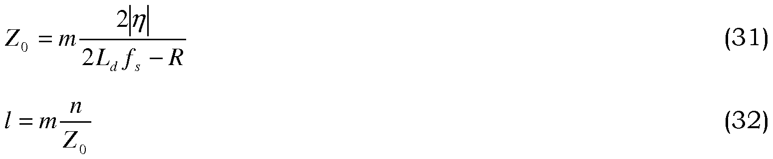
  • a parameter estimator 235 calculates the adaptive parameters Zo and I as follows:
  • m is a parameter used to satisfy equation (30), and can be between 1- 1.6, and preferably 1. 1 - 1.2, which means 10% ⁇ 20% larger than the minimum value of Zo.
  • the parameter m is a testing- tuned coefficient to provide margin for the adaptive parameters Zo and I.
  • Equation (5) indicates that the magnitude of the extended back EMF ⁇ is a function of the currents id and 3 ⁇ 4 as well as the rotor speed r. In steady state diq/ dt can be assumed 0. Thus, if the current id and the speed r are known, the value of ⁇ can be determined.
  • the back EMF magnitude estimator 230 determines the current id from the torque command T cm d.
  • a generated electromagnetic torque T e can be expressed as: l(L d - L q )i d + m ] (33) where p 0 is the number of magnetic pole pairs of the motor 155.
  • the relationship between id and 3 ⁇ 4 depends on the control algorithm used for the motor 155. For example, if a maximum torque per ampere (MTPA) control is used, the relationship between id and 3 ⁇ 4 can be obtained by taking Taylor's series expansion as follows:
  • the back EMF magnitude estimator 230 can determine the values of id and 3 ⁇ 4 using equations (33) and (34) .
  • the relationship between the command torque T cm d and currents id and 3 ⁇ 4 can be implemented by using a look-up table or a high-order polynomial.
  • the back EMF magnitude estimator 230 and the parameter estimator 235 may be software executed by digital signal processor or microcontroller, for example, to implement the EMF estimations and parameter estimations.
  • the back EMF magnitude estimator 230 and the parameter estimator 235 may be executed by the data processor 264.
  • FIG. 2D illustrates an example embodiment of a portion of the QSMO 170 shown in FIG. 1A.
  • a portion 170c includes the switching block 2 10 and sliding mode current estimator 205.
  • the QSMO 170a, shown in FIG. 2A may include the portion 170c and the portion 170c is illustrated to show an example embodiment of how the adaptive parameters Zo and I may be determined by the QSMO 170.
  • the portion 170c is the same as the portion 170b except the portion 170c includes a parameter LUT 240 instead of the back EMF magnitude estimator 230 and the parameter estimator 235.
  • the parameter LUT 240 receives the torque command T cm d and speed command ⁇ * .
  • the parameter LUT 240 is a 3-D lookup table. Based on equation (30), the parameter LUT 240 generates the adaptive parameters Zo and I as follows:
  • the product of QSMO gain I and adaptive parameter Zo are determined based on machine speed and torque command.
  • the QSMO gain I is a constant value, e.g. , 8000, for 5000 Hz sampling frequency.
  • FIG. 2E illustrates an example embodiment of the parameter
  • FIG. 2E illustrates a 3-D lookup table. Based on the torque percentage Torq_Perc and the speed command co r * , the parameter LUT 240 may determine the product of QSMO gain I and adaptive parameter Zo.
  • portion 2 100 represents a product between 200,000 and 400,000
  • portion 2200 represents a product between 400,000 and 600,000
  • portion 2300 represents a product between 600,000 and 800,000
  • portion 2400 represents a product between 800,000 and 1 ,000,000
  • portion 2500 represents a product between 1 ,000,000 and 1 ,200,000.
  • FIG. 2C the observer parameters (Zo and Z) are selected according to the command torque and speed, to manage both load/ speed variation and machine parameter variation from given values provided by a machine manufacturer.
  • the QSMO 170 achieves accurate position estimation without phase shift. While FIGS. 2C-2D illustrate the back EMF estimator 230 as configured to receive the torque command T cm d and the command speed ⁇ * , the percentage Torq_Perc may be directly used from the torque processor 1 15 instead of the torque command T cm d and the command speed ⁇ * .
  • the QSMO 170 is configured to sample the voltage command ⁇ ⁇ * ⁇ and the measured current ⁇ ⁇ at twice a frequency as the PWM frequency of the pulse width generation module 145.
  • a PWM frequency of 6,000 Hz is a relatively low switching frequency compared with 20 kHz.
  • the QSMO 170 with 6,000 Hz sampling frequency has good performance to limit a rotor position error within 3 electric degrees.
  • the sampling frequency is incremented.
  • FIG. 3 illustrates a method of estimating a rotor position in a motor according to an example embodiment. More specifically, FIG. 3 illustrates a method of estimating a rotor position in a motor.
  • the method includes obtaining a measured current for the motor, determining an estimated current using a sliding mode observer, determining a difference between the measured current and the estimated current, generating a switching control vector based on the difference and adaptive parameters of the sliding mode observer, and estimating the rotor position based on the switching control vector.
  • the method of FIG. 3 may be in implemented in a sensorless drive system such as the drive system 100, shown in FIG. 1.
  • the drive system generates a measured current.
  • the current transducers 180a, 180b measure current data ia and ib, respectively, applied to the motor 155.
  • the converter 160 may apply a Clarke transformation or other conversion equations (e.g., certain conversion equations that are suitable are known to those of ordinary skill in the art) to convert the measured three-phase representations of current into two-phase representations of current based on the three-phase current data ia and ib from the current transducers 180a, 180b and an estimated rotor position 6 re from the QSMO 170.
  • the output of the converter 160 module ( i sd , i sq ) is coupled to the current regulator 135.
  • the converter 165 may apply a Park transformation or other conversion equations (e.g., certain conversion equations that are suitable are known to those of ordinary skill in the art) to convert the measured three-phase representations of current into two-phase representations of current based on the current data ia and ib from the current transducers 180a, 180b.
  • a Park transformation or other conversion equations e.g., certain conversion equations that are suitable are known to those of ordinary skill in the art
  • the QSMO 170 receives the measured currents ⁇ ⁇ , ⁇ ⁇ and the voltage commands v * and ⁇ ⁇ * .
  • a QSMO determines an estimated current at S320.
  • the QSMO 170a generates estimated current value ⁇ ⁇ [ i a and i ) based on the voltage command ⁇ ⁇ * ⁇ ( v « an d ⁇ * ) and the switching control vector ⁇ ⁇ ⁇ .
  • the QSMO determines a difference between the measured current and the estimated current.
  • the comparator 207 receives the measured currents ia and i and the estimated current values i a and i p .
  • the comparator 207 determines errors « and between the measured currents ia and ⁇ and the estimated currents i a and i p , respectively.
  • the errors Za and may be differences between the measured currents ia and zjp and the estimated currents i a and i p , respectively.
  • the QSMO generates a switching control vector based on the difference and adaptive parameters of the QSMO.
  • the switching block 2 10 implements a variable switching function where Zo is an adaptive parameter.
  • FIG. 2B illustrates an example embodiment of the variable switching function implemented by the switching block 2 1 .
  • the switching block 2 10 if the tracking error z[k ⁇ is larger than Zo, the switching block 2 10 outputs Zo as the switching control vector Zap, and if the tracking error [/c] is smaller than -Zo, the switching block 2 10 outputs - Zo as the switching control vector Zap . If the tracking error z[k] is limited in a boundary layer between - Zo and Zo, the output of saturation function will be the tracking error [/c] as the switching control vector Zap.
  • the switching block 2 10 outputs the switching control vector Zap to the sliding mode current estimator 205 and the low-pass filter 2 15.
  • condition (i) provides a lower boundary for the product of the gain I and the adaptive parameter Zo; while condition (ii) provides an upper boundary for the product of the gain I and the adaptive parameter Zo.
  • the QSMO estimates the rotor position based on the switching control vector at S350.
  • the position calculator 220 determines a rotor position of the motor 155 based on the estimated back EMF ⁇ ⁇ .
  • the rotor position determined by the position calculator 220 is not compensated for the phase shift caused by the low-pass filter 215. Therefore, the phase shift compensator 225 adds a phase shift 0 re to the rotor position at the logic unit 227 to compensate for the phase shift.
  • the sum of the output from the position calculator 220 and the phase shift A0 re is the estimated rotor position 6 re .
  • the controller e.g., 102
  • the controller may control the motor based on the estimated rotor position.
  • a loop from the current regulator 135 to the inverter 150, to the QSMO 170 and back to the current regulator 135 may be referred to an inner position feedback loop.
  • QSMO 170, the controller 102 and motor 155 are coupling with each other.
  • the output of the QSMO 170 is the estimated rotor position 6 re without any reference value, and the estimated rotor position 0 re is used by the converters 140 and 160.
  • the pulse width generation module 145 receives the transformed voltage commands v * and ⁇ ⁇ * , which are used to generate three phase voltages/ currents for the motor 155.
  • the QSMO 170 receives the measured currents 3 ⁇ 4 and zjp and voltage commands v * and ⁇ ⁇ * , as input.
  • FIG. 1A shows a high order, nonlinear, and highly coupled system including error propagation and self-exciting oscillation.
  • the drive system 100 is configured to implement the speed aided stabilizers.
  • the speed aided stabilizers are based on the idea that motor rotor speed changes much slower than the position changes in medium and high speed ranges.
  • speed can be assumed as a constant value, and can be used to predict the position for a next sample. This predicted position for a next sample can be used as a reference to adjust the estimated position, so as to help the drive system 100 go through the transient with high accuracy.
  • FIGS. 4A-4C illustrate an implementation of a speed buffer for a speed aided stabilizer, according to an example embodiment.
  • FIG. 4D illustrates a structure of the speed buffer implemented in DSP RAM.
  • the QSMO 170 determines an estimated rotor position ⁇ [n] for every PWM cycle having a period of T s [n] .
  • a controller 400 is shown.
  • the controller 400 is the same as the controller 102 except the controller 400 includes a comparator 402 and a delay 405. While the comparator 402 and the delay 405 are illustrated as outside of the QSMO 170, it should be understood that the comparator 402 and the delay 405 may be implemented as a part of the QSMO 170.
  • the QSMO 170 supplies the estimated rotor position to the comparator 402 and the delay 405.
  • the delay 405 delays the estimated rotor position ⁇ [n] and outputs the delayed rotor position to the comparator 402, which is the estimated rotor position in the previous sample.
  • the comparator 402 determines a difference
  • ⁇ [n] between a current estimated rotor position ⁇ [n] and a subsequent estimated rotor position ⁇ [ ⁇ + 1 ⁇ .
  • the difference ⁇ [n] represents a position change.
  • the comparator 402 and the delay 405 may be software used executed by a digital signal processor or microcontroller.
  • the comparator 402 and the delay 405 may be software executed by the data processor 264.
  • the difference ⁇ [n] and associated time period T s [n] are sent to and stored in a speed buffer 410.
  • the speed buffer 410 may be stored in DSP RAM 415 or any other known type of tangible computer readable medium that is configured to be executed by a digital signal processor or microcontroller, for example.
  • Fig. 4C illustrates the speed buffer 410 in more detail. As shown, the speed buffer stores the difference ⁇ [n] and associated time period T s [n] and indexes the values according to n.
  • the buffer 410 is a rolling buffer, which means if a new position change ⁇ [n] is obtained, it will stored at buffer[0] , and original buffer[0] ⁇ buffer[N-2] will be shift right, and become stored at buffer[ l ] ⁇ buffer[N- l ] . Previous information stored in buffer [N- l ] will be lost.
  • N is the buffer size. The buffer size N may be determined based on the speed response, for example. If the size of the buffer 410 is small, the speed response will be fast, however, the estimated speed normally has larger oscillation. If the buffer size is large, the speed will be filtered smoothly, however, the speed response will be slower.
  • an output of the speed buffer 410 becomes similar to a moving average. More specifically, for each PWM cycle, the speed calculator 175 divides a sum of the differences stored in the speed buffer by a sum of the time periods. The speed calculator
  • an estimated speed ⁇ [n] based on estimated position ⁇ [n] can be expressed as:
  • the speed error between estimated and measured speed may be smaller than 1%.
  • FIGS. 5 and 6 illustrate methods of estimating a position of a rotor in a motor.
  • the methods include determining a first estimated position of the rotor using a first algorithm, determining a second estimated position of the rotor using a second algorithm, the second algorithm being different than the first algorithm, determining a first error based on the first estimated position and the second estimated position and determining a third estimated position of the rotor based on the first error.
  • the drive system 100 includes a controller configured to, determine a first estimated position of the rotor using a first algorithm, determine a second estimated position of the rotor using a second algorithm, the second algorithm being different than the first algorithm, determine a first error based on the first estimated position and the second estimated position, and determine a third estimated position of the rotor based on the first error.
  • FIG. 5 illustrates a first method of stabilizing speed according to an example embodiment.
  • the speed stabilizer determines if drive is enabled. If drive is not enabled, the speed stabilizer sets a selected position (third estimated position) ⁇ [n] and a second estimated position ⁇ 2 [ ⁇ ] to equal a first estimated position .
  • the first estimated position is the estimated rotor position output from the QSMO 170. The speed stabilizer returns to S505 to monitor if drive is enabled.
  • the QSMO 170 supplies the first estimated position at S515 and the speed stabilizer determines a first error ⁇ [ ⁇ ] at S520.
  • the speed stabilizer determines the first error ⁇ [ ⁇ ] by determining an absolute value of a difference between the second estimated position ⁇ 2 [ ⁇ ] and the first estimated position .
  • the speed stabilizer determines if the position error is smaller than the error margin E.
  • the error margin E indicates whether the QSMO 170 is stable. If the speed stabilizer determines that the first error ⁇ [ ⁇ ] is less than the error margin E, then the speed stabilizer sets the selected estimated position ⁇ [n] as the output of the QSMO , at S530. If the first error ⁇ [ ⁇ ] is larger than the error margin E, which means QSMO 170 is unstable or large transient occurs, then the speed stabilizer sets the selected estimated position
  • the controller controls the motor based on the selected estimated position ⁇ [n] .
  • the speed stabilizer determines a second estimated position ⁇ 2 [ ⁇ ] for a next PWM cycle based on a speed prediction algorithm.
  • the second estimated position ⁇ 2 [ ⁇ ] may be determined by the speed stabilizer as:
  • the error margin E is a design parameter that is determined based on empirical data.
  • FIG. 6 illustrates a second method of stabilizing speed according to an example embodiment. It should be understood that the QSMO 170 is configured to implement the method shown in FIG. 6.
  • the speed stabilizer implements a position error rolling sum ⁇ £[n] .
  • the position error rolling sum ⁇ [ ⁇ ] adds each sample error ⁇ [ ⁇ ] between ⁇ 2 [ ⁇ ] and together.
  • the position error rolling sum £[n] may be referred to as the first error.
  • the speed stabilizer determines if drive is enabled. If drive is not enabled, the speed stabilizer sets a selected position (third estimated position) ⁇ [n] and the second estimated position ⁇ 2 [ ⁇ ] equal the first estimated position The first estimated position is the estimated rotor position output from the QSMO 170. The speed stabilizer returns to S605 to monitor if drive is enabled.
  • the QSMO 170 supplies the first estimated position at S615 and the speed stabilizer determines a current error ⁇ [ ⁇ ] at S620.
  • the speed stabilizer determines the current error ⁇ [ ⁇ ] by determining an absolute value of a difference between the second estimated position ⁇ 2 [ ⁇ ] and the first estimated position
  • the speed stabilizer determines if the current error ⁇ [ ⁇ ] is smaller than an error margin for a single sample E .
  • the error margin E indicates whether the QSMO 170 is stable. If the speed stabilizer determines that the current error ⁇ [ ⁇ ] is larger than the error margin for a single sample E , then the speed stabilizer sets the selected the second estimated position ⁇ 2 [ ⁇ ] , at S630.
  • the speed stabilizer adds the current error ⁇ [ ⁇ ] to a sum of previous errors ⁇ [ ⁇ - ⁇ ] to determine the position error rolling
  • the speed stabilizer determines if the position error rolling sum is smaller than the error margin E.
  • the error margin E indicates whether the QSMO 170 is stable. If the speed stabilizer determines that the position error rolling sum is less than the error margin E, then the speed stabilizer sets the selected estimated position ⁇ [n] as the output of the QSMO at S645. If position error rolling sum is larger than the error margin E, which means QSMO 170 is unstable or large transient occurs, then the speed stabilizer sets the selected estimated position ⁇ [n] as second estimated position ⁇ 2 [ ⁇ ] minus the position error rolling sum
  • the controller controls the motor based on the selected estimated position ⁇ [n] .
  • the speed stabilizer determines a second estimated position ⁇ 2 [ ⁇ ] for a next PWM cycle based on a speed prediction algorithm.
  • the step S660 is the same as S550 and, thus, will not be described in greater detail for the sake of clarity.
  • the error margin for a single sample £ is a small value, and normally generally within 0.5 electric degree. Moreover, the error margin E may be selected as 3 electric degrees.
  • QSMO Quasi-SMO
  • EMF extended back electromagnetic force
  • a discrete-time sliding mode observer with conventional switching functions, e.g., a sign function, will keep tight regulation to force the state trajectory close to the sliding surface even when tracking error is within the width of the boundary layer. This could cause a chattering problem during steady state.
  • a switching function may be implemented. The switching function leads to a quasi-sliding mode motion of the DSMO at steady state. Since the magnitude of the extended back EMF of the IPMSM changes with both load and speed variations, the parameters allow better performance than conventional SMOs.
  • At least another example embodiment discloses speed aided stabilizers to improve the drive system stability and help the drive system go through smoothly at load/ speed transients.
  • the speed aided stabilizers are based on the idea that motor rotor speed changes much slower than the position changes in medium and high speed ranges.
  • speed can be assumed as a constant value, and can be used to predict the position for a next sample. This predicted position for a next sample can be used as a reference to adjust the estimated position, so as to help the system go through the transient with high accuracy.

Landscapes

  • Engineering & Computer Science (AREA)
  • Power Engineering (AREA)
  • Control Of Ac Motors In General (AREA)
  • Control Of Motors That Do Not Use Commutators (AREA)
  • Control Of Electric Motors In General (AREA)

Description

DRIVE SYSTEMS INCLUDING SLIDING MODE OBSERVERS AND METHODS OF CONTROLLING THE SAME
FIELD
Example embodiments are related to electric drive device systems and/ or methods for controlling electric drive devices such as Interior Permanent Magnet (IPM) motors or machines.
BACKGROUND IPM synchronous motors (IPMSMs) are used in hybrid and electric vehicle systems. Rotor position of the IPMSM is used for high- performance traction or voltage control of the IPMSM.
Electromechanical type of position sensors, e.g., resolvers, optical encoders, and hall-effect sensors, are used to obtain the rotor position and/or speed in IPMSM drive systems. The use of these electromechanical sensors increases cost, size, weight, and hardware wiring complexity of the IPMSM drive systems. Moreover, mounting electromechanical sensors on a rotor of the motor affects the robustness of the IPMSM. Sensors are often subject to failures in harsh environments, such as excessive ambient temperature, super high-speed operation, and other adverse or heavy load conditions.
As an alternative to sensors, sensorless drives including observers are used. One type of an art recognized observer is a sliding mode observer (SMO). A SMO is embodied in a specific purpose computer, mainly a microcontroller or digital signal processor specifically programmed to execute the SMO. In general, a SMO is an observer having inputs that are discontinuous functions of an error between estimated and measured outputs. In a SMO, a manifold is designed such that a system state trajectory exhibits a certain behavior when confined to the manifold. The manifold may also be referred to as a sliding surface. SUMMARY
At least one example embodiment discloses an adaptive Quasi- SMO (QSMO) to estimate the rotor position from extended back electromagnetic force (EMF) quantities in an IPMSM. The QSMO parameters are adaptive to the load and rotor speed.
At least one example embodiment discloses an extended back EMF-based adaptive QSMO for rotor position estimation for a sensorless IPMSM drive. In the context of the present application, a sensorless system is a position/ speed sensorless system, where position sensors may not be used to measure rotor position.
In the present application, state trajectory may refer to a difference between measured current and estimated current.
The inventors have discovered that a discrete-time sliding mode observer (DSMO) with conventional switching functions will keep tight regulation to force the state trajectory close to the sliding surface even when tracking error is within the width of the boundary layer. This could cause a chattering problem during a steady state. To mitigate this chattering problem and achieve a bounded motion within a limited boundary layer, a switching function may be implemented. The switching function leads to a quasi-sliding mode motion of the DSMO at steady state. Since the magnitude of the extended back EMF of the IPMSM changes with both load and speed variations, the parameters allow better performance than conventional SMOs.
At least another example embodiment discloses speed aided stabilizers to improve drive system stability and help the drive system go smoothly at load/ speed transients. The inventors have discovered that commonly used methods to improve the stability are system state decoupling, which are used to disconnect direct input/ output relationship between each sub-system. However, a second order IPMSM model is a simplified model and d-q axis equations are also coupling with each other. The inductances change with stator current and a gamma angle, and the stator resistance changes with temperature. These parameter variations are difficult to accurately model in a machine model. For other modules in a close-loop system, the inverter and SMO are nonlinear, and linearization methods as well as other approximation methods are needed. So the whole sensorless control system is a high order, nonlinear, coupling system with unmodeled parameters and model uncertainties. The transfer function and pole placement based decoupling methods are difficult for both analysis and implementation.
The speed aided stabilizers are based on the idea that motor rotor speed changes much slower than the position changes in medium and high speed ranges. Thus, during the time interval of consecutive two sampling points, speed can be assumed as a constant value, and can be used to predict the position for a next step. This predicted position for a next step can be used as a reference to adjust the estimated position, so as to help the system go through the transient with high accuracy.
At least one example embodiment discloses a drive system including a motor including a rotor, the motor configured to receive a measured current, a controller configured to generate a voltage command for the motor, a sliding mode observer configured to determine an estimated current for the motor based on the voltage command, determine a difference between the measured current and the estimated current, and determine a switching control vector and an estimator configured to estimate a rotor position based on the switching control vector, the switching control vector being determined based on the difference and adaptive parameters of the sliding mode observer, the controller being further configured to control the motor based at least in part on the estimated rotor position.
In one example embodiment, the sliding mode observer is configured to sample the measured current at a frequency of less than 10 kHz. In one example embodiment, the sliding mode observer is configured to sample the measured current at approximately 6 kHz.
In one example embodiment, the sliding mode observer comprises the estimator.
In one example embodiment, the controller is configured to drive the motor between 500 revolutions per minute (RPM) and 5000 RPM.
In one example embodiment, the sliding mode observer is configured to determine the switching control vector by
Z0 £[k] > Z0
£[k] - Z0 < e[k] < Z{
<*β ~
-Z0 £[k] < -Z0
wherein Ζαβ is the switching control vector, e[k] is the difference and Zo is one of the adaptive parameters.
In one example embodiment, Zo is
2\η\
Z0 >
2Ld fs - R wherein Ld is a direct axis inductance of the motor, fs is a sampling frequency, η is a magnitude of extended back electromagnetic force (EMF) of the motor and R is a resistance of a stator of the motor.
In one example embodiment,
Figure imgf000006_0001
wherein a is between 1. 1 and 1.2.
In one example embodiment, the sliding mode observer is configured to determine an extended back electromagnetic force (EMF) of the motor and Z0 is proportional to a magnitude of the extended back EMF of the motor.
In one example embodiment, the sliding mode observer is configured to produce a gain and a product of the gain and 0 is larger than the magnitude of the extended back EMF of the motor.
In one example embodiment, the sliding mode observer is configured to receive a command speed for the motor and an associated torque percentage and the sliding mode observer includes a three-dimensional lookup table configured to determine Zo based on the command speed and the torque percentage.
In one example embodiment, the drive system further includes an inverter configured to supply a three-phase current to the motor based on pulse width modulation (PWM).
In one example embodiment, the sliding mode observer is configured to estimate a rotor position at a sampling frequency relatively greater than a PWM frequency.
In one example embodiment, the sliding mode observer is configured to estimate a rotor position at a sampling frequency double the PWM frequency.
In one example embodiment, the controller is configured to generate a voltage command and the sliding mode observer is configured to determine the estimated current based on the voltage command and the measured current.
At least one example embodiment discloses a method of estimating a rotor position in a motor. The method includes, obtaining a measured current for the motor, determining an estimated current using a sliding mode observer, determining a difference between the measured current and the estimated current, generating a switching control vector based on the difference and adaptive parameters of the sliding mode observer, and estimating the rotor position based on the switching control vector. In one example embodiment, the method further includes sampling the measured current a frequency of less than 10 kHz, wherein the determining of a difference determines the difference based on the sampled current.
In one example embodiment, the sampling samples the measured current at approximately 6 kHz.
In one example embodiment, the method further includes driving the motor between 500 revolutions per minute (RPM) and 5000 RPM.
At least another example embodiment discloses a sliding mode observer configured to receive a measured current for a motor, determine an estimated current for a motor, determine a difference between the measured current and the estimated current, determine a switching control vector, and estimate a rotor position based on the switching control vector, the switching control vector being determined based on the difference and adaptive parameters of the sliding mode observer.
At least another example embodiment discloses a method of estimating a rotor position in a motor in a sensorless drive system. The method includes generating a measured current for the motor, determining an estimated current using a sliding mode observer, determining a difference between the measured current and the estimated current, generating a switching control vector based on the difference and adaptive parameters of the sliding mode observer, estimating the rotor position based on the switching control vector, and controlling the motor based on the estimating.
BRIEF DESCRIPTION OF THE DRAWINGS
Example embodiments will be more clearly understood from the following detailed description taken in conjunction with the accompanying drawings. FIGS. 1A-6 represent non-limiting, example embodiments as described herein.
FIG. 1A illustrates a drive system for controlling an IPM machine according to an example embodiment;
FIG. IB illustrates a data processing system of the drive system of FIG. 1A according to an example embodiment;
FIG. 2A illustrates an example embodiment of a QSMO shown in FIG. 1A;
FIG. 2B illustrates an example embodiment of a variable switching function implemented by a switching block according to an example embodiment;
FIG. 2C illustrates an example embodiment of a portion of the QSMO shown in FIG. 1A;
FIG. 2D illustrates an example embodiment of a portion of the QSMO shown in FIG. 1A;
FIG. 2E illustrates an example embodiment of a parameter lookup table;
FIG. 3 illustrates a method of estimating a rotor position in a motor according to an example embodiment;
FIGS. 4A-4D illustrate an implementation of a speed buffer for a speed aided stabilizer, according to an example embodiment;
FIG. 5 illustrates a first method of stabilizing speed according to an example embodiment; and
FIG. 6 illustrates a second method of stabilizing speed according to an example embodiment.
DETAILED DESCRIPTION
Various example embodiments will now be described more fully with reference to the accompanying drawings in which some example embodiments are illustrated.
Accordingly, while example embodiments are capable of various modifications and alternative forms, embodiments thereof are shown by way of example in the drawings and will herein be described in detail. It should be understood, however, that there is no intent to limit example embodiments to the particular forms disclosed, but on the contrary, example embodiments are to cover all modifications, equivalents, and alternatives falling within the scope of the claims. Like numbers refer to like elements throughout the description of the figures.
It will be understood that, although the terms first, second, etc. may be used herein to describe various elements, these elements should not be limited by these terms. These terms are only used to distinguish one element from another. For example, a first element could be termed a second element, and, similarly, a second element could be termed a first element, without departing from the scope of example embodiments. As used herein, the term "and/ or" includes any and all combinations of one or more of the associated listed items.
It will be understood that when an element is referred to as being "connected" or "coupled" to another element, it can be directly connected or coupled to the other element or intervening elements may be present. In contrast, when an element is referred to as being "directly connected" or "directly coupled" to another element, there are no intervening elements present. Other words used to describe the relationship between elements should be interpreted in a like fashion (e.g., "between" versus "directly between," "adjacent" versus "directly adjacent," etc.) .
The terminology used herein is for the purpose of describing particular embodiments only and is not intended to be limiting of example embodiments. As used herein, the singular forms "a," "an" and "the" are intended to include the plural forms as well, unless the context clearly indicates otherwise. It will be further understood that the terms "comprises," "comprising," "includes" and/ or "including," when used herein, specify the presence of stated features, integers, steps, operations, elements and/ or components, but do not preclude the presence or addition of one or more other features, integers, steps, operations, elements, components and/ or groups thereof.
It should also be noted that in some alternative implementations, the functions/ acts noted may occur out of the order noted in the figures. For example, two figures shown in succession may in fact be executed substantially concurrently or may sometimes be executed in the reverse order, depending upon the functionality/ acts involved.
Unless otherwise defined, all terms (including technical and scientific terms) used herein have the same meaning as commonly understood by one of ordinary skill in the art to which example embodiments belong. It will be further understood that terms, e.g., those defined in commonly used dictionaries, should be interpreted as having a meaning that is consistent with their meaning in the context of the relevant art and will not be interpreted in an idealized or overly formal sense unless expressly so defined herein.
Portions of example embodiments and corresponding detailed description are presented in terms a processor specifically programmed to execute software, or algorithms and symbolic representations of operation on data bits within a computer memory. These descriptions and representations are the ones by which those of ordinary skill in the art effectively convey the substance of their work to others of ordinary skill in the art. An algorithm, as the term is used here, and as it is used generally, is conceived to be a self-consistent sequence of steps leading to a result. The steps are those requiring physical manipulations of physical quantities. Usually, though not necessarily, these quantities take the form of optical, electrical, or magnetic signals capable of being stored, transferred, combined, compared, and otherwise manipulated. It has proven convenient at times, principally for reasons of common usage, to refer to these signals as bits, values, elements, symbols, characters, terms, numbers, or the like. In the following description, illustrative embodiments will be described with reference to acts and symbolic representations of operations (e.g., in the form of flowcharts) that may be implemented as program modules or functional processes including routines, programs, objects, components, data structures, etc., that perform particular tasks or implement particular abstract data types and may be implemented using existing hardware. Such existing hardware may include one or more Central Processing Units (CPUs), digital signal processors (DSPs), application-specific-integrated-circuits, field programmable gate arrays (FPGAs) computers or the like.
It should be borne in mind, however, that all of these and similar terms are to be associated with the appropriate physical quantities and are merely convenient labels applied to these quantities. Unless specifically stated otherwise, or as is apparent from the discussion, terms such as "processing" or "computing" or "calculating" or "determining" or "displaying" or the like, refer to the action and processes of a computer system, or similar electronic computing device, that manipulates and transforms data represented as physical, electronic quantities within the computer system's registers and memories into other data similarly represented as physical quantities within the computer system memories or registers or other such information storage, transmission or display devices.
Note also that the software implemented aspects of example embodiments are typically encoded on some form of tangible (or recording) storage medium or implemented over some type of transmission medium. The tangible storage medium may be magnetic (e.g., a floppy disk or a hard drive) or optical (e.g., a compact disk read only memory, or "CD ROM"), and may be read only or random access.
In a discrete-time sliding mode controller (DSMC) or observer, to facilitate DSP or micro-controller based applications, controller inputs are calculated once per sampling period and held constant during this interval. The inventors have discovered that due to a finite sampling period or PWM switching frequency, the state trajectory is difficult to precisely move along the sliding surface, which will lead to a quasi- sliding mode motion only. For IPMSM drive applications, limitations in control loop frequency and CPU loading make it challenging to achieve high accuracy in position estimation. Moreover, a magnitude of extended back electromagnetic force (EMF) contains both a speed- related term and current-related terms, which means that both load and speed will affect the magnitude of the extended back EMF.
At least one example embodiment discloses an adaptive Quasi- SMO (QSMO) to estimate the rotor position from the extended back electromagnetic force (EMF) quantities in an IPMSM. The QSMO parameters are adaptive to the load and rotor speed.
FIGS. 1A-2D illustrate a drive system including a motor having a rotor, the motor configured to receive a measured current, a controller configured to generate a voltage command for the motor, a sliding mode observer configured to determine an estimated current for the motor based on the voltage command, determine a difference between the measured current and the estimated current, and determine a switching control vector and an estimator configured to estimate a rotor position based on the switching control vector, the switching control vector being determined based on the difference and adaptive parameters of the sliding mode observer. The controller is configured to control the motor based at least in part on the estimated rotor position
In accordance with an example embodiment, FIG. 1A illustrates a drive system 100 for controlling an IPM machine such as a motor 155 (e.g., an interior permanent magnet synchronous motor (IPMSM)) or another alternating current machine. The drive system 100 may also be referred to as an IPMSM drive system.
It should be understood that the drive system 100 may include additional features that are not illustrated in FIG. 1A. For example, the drive system 100 may include a rotor magnet temperature estimation module, a current shaping module, and a terminal voltage feedback module. The features shown in FIG. 1A are illustrated for the convenience of describing the drive system 100 and it should be understood that the drive system 100 should not be limited to the features shown in FIG. 1A.
The system 100 includes electronic modules, software modules, or both. In an example embodiment, the drive system 100 includes an electronic data processing system 101 to support storing, processing or execution of software instructions of one or more software modules. The electronic data processing system 101 is indicated by the dashed lines in FIG. 1A and is shown in greater detail in FIG. IB.
The data processing system 101 is coupled to an inverter circuit 150. The inverter circuit 150 may be a three-phase inverter. The inverter circuit 150 includes a semiconductor drive circuit that drives or controls switching semiconductors (e.g., insulated gate bipolar transistors (IGBT) or other power transistors) to output control signals for the motor 155. In turn, the inverter circuit 150 is coupled to the motor 155. The motor 155 is associated with sensors 180a and 180b.
Throughout the specification, the sensors 180a and 180b are referred to as current transducers. However, it should be understood that the sensors 180a and 180b may be another type of current sensor.
The current transducers 180a and 180b and the motor 155 are coupled to the data processing system 101 to provide feedback data (e.g., current feedback data, such as phase current values ia and ib), raw position signals, among other possible feedback data or signals, for example. While only two current transducers 180a and 180b are shown, it should be understood that the driver system 100 may implement three current transducers.
The data processing system 101 includes a software controller 102, converters 160, 165, a pulse width generation module 145, a QSMO 170 and a speed calculator 175.
The software controller 102, converters 160, 165, the pulse width generation module 145, the QSMO 170 and the speed calculator 175 are software modules. While the software controller 102, converters 160, 165, the pulse width generation module 145, the QSMO 170 and the speed calculator 175 are described as executing functions, it should be understood that a data processor, such as a digital signal processor or a microcontroller, is specifically programmed to execute the software controller 102, converters 160, 165, the pulse width generation module 145, the QSMO 170 and the speed calculator 175. For example, a data processor 264 is specifically programmed to execute the software controller 102, converters 160, 165, the pulse width generation module 145, the QSMO 170 and the speed calculator 175, as will be described in FIG. IB.
The controller 102 includes a speed regulator 105, a base torque lookup table (LUT) 1 10, a torque processor 1 15, a ratio calculator 120, a q-axis current (iq) command LUT 125, a d-axis current (id) command LUT 130, a current regulator 135, a voltage compensator 137 and a converter 140.
In an example embodiment, a speed regulator 105 receives input data representing a difference between an estimated rotor speed (br and a command rotor speed cor * as input.
The command rotor speed a>r * may be input by a controller (shown as 266 in FIG. IB) via a vehicle data bus 1 18. For example, if an operator wants the motor 155 to run at 5,000 RPM, the operator inputs 5,000 RPM into the controller and the vehicle data bus 1 18 inputs the command rotor speed ωτ to the controller 102. The speed regulator 105 converts the received input data into a torque command Tcmd.
While the term command is used throughout the specification, it should be understood that command refers to a target value. The base torque LUT 1 10 determines a base torque value Tbase based on the estimated rotor speed cor .
From the estimated rotor speed γ , base torque values are respectively associated with discrete speed points with a nominal dc bus voltage level. In other words, the two-dimensional base torque LUT 1 10 is established from a motor characterization procedure. During the IPM motor characterization procedure, each rotor shaft speed has a maximum output torque, which is defined as the base torque at that speed. Thus, the base torque may also be referred to as peak torque.
The base torque LUT 1 10 outputs the associated base torque value as the base torque value Tbase to the torque processor 1 15.
The torque processor 1 15 receives the base torque value Tbase and the torque command Tcmd. The torque command Tcmd may be in Nm.
The torque processor 1 15 is configured to determine an absolute value of the torque command Tcmd. The torque processor 1 15 is configured to convert the absolute value of the torque command Tcmd into a percentage Torq_Perc of the base torque value Tbase. The torque processor 1 15 outputs the percentage Torq_Perc to the q-axis current (iq) command LUT 125 and the d-axis current (id) command LUT 130.
In addition to sending the estimated rotor speed cbr to the base torque LUT 1 10, the speed calculator 175 sends the estimated rotor speed cor to the ratio calculator 120.
In addition to receiving the estimated rotor speed cbr , the ratio calculator 120 is configured to receive the measured operating dc bus voltage value. The measured operating dc bus voltage value is provided by a voltage sensor 185 which measures the DC bus in the inverter circuit 150. The inverter circuit 150 is powered by a direct current (dc) voltage bus. The ratio calculator 120 adjusts the operating DC bus voltage VDC by the voltage sensor 185 to the detected operating rotor shaft speed ratio as follows:
1 ratio — (i)
where Tratio is the adjusted detected operating DC bus voltage to the detected operating rotor shaft speed ratio and Y is a coefficient. For example, the coefficient Y may be 0.9. The ratio Tratio is output by the ratio calculator 120 to the d-q axis current command LUTs 125 and 130.
The q-axis current command (iq) LUT 125 and the d-axis current command (id) LUT 130 are configured to receive the ratio Tratio. The q-axis current command LUT 125 and the d-axis current command LUT 130 store q-axis and d-axis current commands, respectively, each of which is associated with a pair of ratio and torque percentage values. The development of the q-axis current command LUT 125 and the d-axis current command LUT 130 may be done using any known method.
The d-q axis current refers to the direct axis current and the quadrature axis current as applicable in the context of vector- controlled alternating current machines, such as the motor 155.
The d-axis current command LUT 130 is configured to output a d-axis current command id * that is associated with the received torque percentage Torq_Perc and the ratio Tratio. As shown in FIG. 1A, the d- axis current command id * is output to the current regulator 135.
The q-axis current command LUT 125 is configured to output a q-axis current command i* that is associated with the received torque percentage Torq_Perc and ratio Tratio.
It should be understood that id * and i* are current commands for a stator of the motor 155.
While the q-axis current command LUT 125 and d-axis current command LUT 130 are illustrated and described as LUTs, it should be understood that the q-axis current command LUT 125 and d-axis current command LUT 130 may be implemented as a set of equations that relate respective torque commands to corresponding direct and quadrature axes currents, or a set of rules (e.g., if-then rules) that relates respective torque commands to corresponding direct and quadrature axes currents.
As shown in FIG. 1A, the q-axis current command i* is output to the current regulator 135.
The current regulator 135 is capable of communicating with the pulse-width modulation (PWM) generation module 145 (e.g., space vector PWM generation module). The current regulator 135 receives respective d-q axis current commands (e.g., id * and i* ) and measured d-q axis currents (e.g., id and is ) for the stator and outputs corresponding pre-compensated d-q axis voltage commands v'd and vq' to a voltage compensator 137.
The voltage compensator 137 provides voltage adjustment data to adjust the pre-compensated d-q axis voltage commands v'd and vq' and outputs d-q axis voltage commands vd * and v* . It should be understood that the voltage compensator 137 may generate the d-q axis voltage commands (e.g., vd * and v* commands) using any known method such as current feed forward compensation.
The converter 140 receives the d-q axis voltage commands vd * and v* and performs an inverse Park transformation to generate α-β axis voltage commands v* and νβ * . While at least one example embodiment is described using the α-β axis, it should be understood that example embodiments may be implemented using the d-q axis or three phase representation of a control vector.
In an example embodiment, the PWM generation module 145 converts the a axis voltage and β axis voltage data (voltage commands v* and νβ * ) from two phase data representations into three phase representations (e.g. , three phase voltage representations, such as va*, vb* and vc*) for control of the motor 155, for example. Outputs of the PWM generation module 145 are coupled to the inverter circuit 150.
The inverter circuit 150 includes power electronics, such as switching semiconductors to generate, modify and control pulse-width modulated signals or other alternating current signals (e.g. , pulse, square wave, sinusoidal, or other waveforms) applied to the motor 155. The PWM generation module 145 provides inputs to a driver stage within the inverter circuit 150. An output stage of the inverter circuit 150 provides a pulse-width modulated voltage waveform or other voltage signal for control of the motor 155. In an example embodiment, the inverter 150 is powered by the direct current (dc) voltage bus voltage VDC
The current transducers 180a, 180b measure two of three phase current data ia and ib, respectively, applied to the motor 155. It should be understood that an additional current transducer may also measure a third phase current data ic.
The converter 160 may apply a Clarke transformation or other conversion equations (e.g. , certain conversion equations that are suitable and are known to those of ordinary skill in the art) to convert the measured three-phase representations of current into two-phase representations of current based on the current data ia and ib from the current transducers 180a, 180b and an estimated rotor position
6re from the QSMO 170. The output of the converter 160 module ( id , iq ) is coupled to the current regulator 135.
The converter 165 may apply a Park transformation or other conversion equations (e.g. , certain conversion equations that are suitable and are known to those of ordinary skill in the art) to convert the measured three-phase representations of current into two-phase representations of current based on the current data ia and ib from the current transducers 180a, 180b. The output of the converter 160 module (measured currents ίαβ) is coupled to the QSMO 170.
The QSMO 170 receives the measured currents ίαβ and the voltage commands v* and νβ * . Based on the measured currents ίαβ and the voltage commands v* and νβ * , the QSMO 170 is configured to output the estimated rotor position 6re to the speed calculator 175 and the converter 160, as will be described in greater detail in FIG. 2.
The speed calculator 175 may convert the estimated rotor position 0re provided by the QSMO 170 into the estimated rotor speed
In FIG. I B, the electronic data processing system 101 includes an electronic data processor 264, a data bus 262, a data storage device 260, and one or more data ports (268, 270, 272 and 274) . The data processor 264, the data storage device 260 and one or more data ports are coupled to the data bus 262 to support communications of data between or among the data processor 264, the data storage device 260 and one or more data ports.
In an example embodiment, the data processor 264 may include an electronic data processor, a digital signal processor, microprocessor, a microcontroller, a programmable logic array, a logic circuit, an arithmetic logic unit, an application specific integrated circuit, a digital signal processor, a proportional-integral-derivative (PID) controller, or another data processing device.
The data storage device 260 may include any magnetic, electronic, or optical device for storing data. For example, the data storage device 260 may include an electronic data storage device, an electronic memory, non-volatile electronic random access memory, one or more electronic data registers, data latches, a magnetic disc drive, a hard disc drive, an optical disc drive, or the like. Moreover, in one example embodiment the data storage device 260 may store the controller 102, pulse width generation module 145, converters 160, 165, the QSMO 170 and the speed controller 175 to be used executed by the data processor 264. The data processor 264 may access the data storage device 260 and execute the controller 102, pulse width generation module 145, converters 160, 165, the QSMO 170 and the speed controller 175 via the data bus 262.
As shown in FIG. IB, the data ports include a first data port 268, a second data port 270, a third data port 272 and a fourth data port 274, although any suitable number of data ports may be used. Each data port may include a transceiver and buffer memory, for example. In an example embodiment, each data port may include any serial or parallel input/ output port.
In an example embodiment as illustrated in FIG. IB, the first data port 268 is coupled to the vehicle data bus 1 18. In turn, the vehicle data bus 1 18 is coupled to a controller 266. In one configuration, the second data port 270 may be coupled to the inverter circuit 150; the third data port 272 may be coupled to the voltage sensor 185; and the fourth data port 274 may be coupled to the transducers 180a and 180b.
In an example embodiment of the data processing system 101 , the speed regulator 105 is associated with or supported by the first data port 268 of the electronic data processing system 101. The first data port 268 may be coupled to a vehicle data bus 1 18, such as a controller area network (CAN) data bus. The vehicle data bus 1 18 may provide data bus messages with torque commands to the speed regulator 105 via the first data port 268. The operator of a vehicle may generate the torque commands via a user interface, such as a throttle, a pedal, the controller 266, or other control device.
FIG. 2A illustrates an example embodiment of the QSMO 170 shown in FIG. 1A. The QSMO 170 is configured to, receive a measured current for a motor, determine an estimated current for a motor, determine a difference between the measured current and the estimated current, determine a switching control vector, and estimate a rotor position based on the switching control vector, the switching control vector being determined based on the difference and adaptive parameters of the sliding mode observer.
The dynamics of the motor 155 can be modeled in the d-q rotating reference frame as:
vd R + pLd -coreLq
(2) wreLd R + pL(
Figure imgf000022_0002
where p is the derivative operator, vsd, vsq, isd, and isq are the stator voltages and currents, respectively, Qre is the rotor electrical speed, and Ψτη is the magnetic flux linkage of the motor 155, Ld and Lq are the d-axis and q-axis inductances, respectively; and R is the stator resistance. As should be understood, core is the rotor electrical speed and ωΓ is the mechanical speed and core is cor multiplied by the pole- pairs number.
Using the inverse Park transformation, the dynamic model of the motor 155 in the α-β stationary reference frame can be expressed as:
L + AL cos(2<9re )
ALsin fl
Figure imgf000022_0003
Figure imgf000022_0001
(3) where L = D Q ; AL = d q ; and Qre is the rotor position angle. While the electrical quantity 0re is used described as the rotor position angle, it should be understood that a mechanical quantity may be used where the mechanical quantity is the electrical quantity 0re divided by a number of magnetic pole pairs p0 of the motor 155.
Due to the saliency of the motor (i.e., Ld≠ Lq) , both the back EMF and the inductance matrix contain the information of the rotor position angle. Moreover, equation (3) contains both 2Qre and 0re terms. To facilitate rotor position observation, an extended back EMF- based model for the motor 155 may be used as follows:
-sin <9re
{L - La ){G)J - piq ) + G)re /m
Figure imgf000023_0001
cos #
(4)
In equation (4) only the extended back EMF term contains the information of the rotor position. Thus, the rotor position can be extracted by an inverse tangent method or angle tracking observer using an estimated extended back EMF.
Back EMF is defined as:
®re n.
cos #.„
Whereas extended back EMF may be defined as:
-sin <9re
(L a , - L q ) /((0 re i a, - p ^i q ) + ω re ψ' m
cos #.„
A magnitude of the extended back EMF may be: η = (Ld - Lq) ( C retd ~ piq) + Οτβψη (5) The dynamic current equations of the motor 155 can be expressed in matrix form: X= AX + BV + E where
Figure imgf000024_0001
which is selected as the system state;
L q - L d. .
L . -
(0„ d L q .
(10) and
Figure imgf000024_0002
Using the first-order Euler method, equation (6) may be written into a discrete-time model as follows:
[k + iR [k +
Figure imgf000024_0003
wherein Ts is the sampling period.
Referring back to FIG. 2A, a QSMO 170a includes a sliding mode current estimator 205, a switching block 210, a low-pass filter 215, a position calculator 220 and a phase shift compensator 225. The QSMO 170a may be executed by a digital signal processor or microcontroller. For example, the QSMO 170a may be software stored in a tangible computer readable medium and executed by the data processor 264.
The QSMO 170a receives the voltage commands va and v and the measured currents ¾ and zjp converted from measured phase currents ¾, ¾ and fc.
The sliding mode current estimator 205 receives the voltage commands v* and νβ * and a switching control vector Ζαβ. It should be understood that terms having "αβ" as subscripts represent a vector having both the a-axis term and the β-axis term. For example, voltage commands v* and νβ * may be represented as να * β such that (ι αβ)τ equals [v* a ι β] .
Using equation (12), the sliding mode current estimator 205 samples the voltage commands v* and νβ * and the switching control vector Ζαβ and generates an estimated current value ί αβ [ i a and ί β ) as follows:
L - L , T R
[k + i] = T 0)„— i„[k] + lZ k] k]
-d j
Figure imgf000025_0001
As should be noted, equation (13) has the same form as equation (12). However, in equation (13), the voltage commands v* a and ν"β are used, which are received from the converter 140, so that the terminal voltage does not need to be measured. However, if a dead-time effect is not fully compensated for, the voltage command will not equal the terminal voltage. This voltage mismatch will bring some error to the estimated position.
A comparator 207 receives the measured currents ia and zjp and the estimated currents i a and i p . The comparator 207 determines errors « and between the measured currents ia and Ζ and the estimated currents i a and i p , respectively. The errors « and may be differences between the measured currents ia and zjp and the estimated currents i a and i p , respectively.
The comparator 207 sends the errors εα and ε to the switching block 210. Based on the errors εα and ε , the switching block 210 determines the switching control vector Ζαβ. The switching control vector Ζαβ contains the information of back EMF. Since the switching control vector Zap is the output of switching block 210, it contains heavy switching noise. The low-pass filter 215 receives the switching control vector Zap to smooth the estimated back EMF profile. The low- pass filter 215 adds a phase delay to original signal input. The phase shift compensator 225 compensates for the phase delay.
Thus, a tracking error between the measured current and estimated current is:
Figure imgf000026_0001
More specifically, equation (15) can be obtained by subtracting (13) from (12):
Figure imgf000026_0002
The QSMO 170a has a sliding surface s[/c], which is designed to equal the tracking error z[k] and 0.
The switching block 210 implements a variable switching function as follows:
Figure imgf000027_0001
where Zo is an adaptive parameter. A boundary layer is formed between -Zo and Zo.
FIG. 2B illustrates an example embodiment of the variable switching function implemented by the switching block 210. As shown in FIG. 2B, if the tracking error [/c] is larger than the adaptive parameter Zo, the switching block 210 outputs Zo as the switching control vector Za§. If the tracking error [/c] is smaller than - Zo, the switching block 210 outputs - Zo as the switching control vector Zap. If the tracking error z[k] is between - Zo and Zo, the output of switching function will be the tracking error [/d . In this case, the tracking error [/c] is the switching control vector Za§. The switching block 210 outputs the switching control vector Zap to the sliding mode current estimator 205 and the low-pass filter 215.
If the reaching condition can be satisfied, the state trajectory will approach the sliding surface. When the tracking error [/c] is limited within a boundary layer (e.g., between - Zo and Zo), the output of the switching block 210 is equal to the extended back EMF with heavy noise. In other words, Za§ equals the extended back EMF with high order harmonics. The determination of the adaptive parameter Zo is described in greater detail below.
It should be understood that the variable switching function may be implemented as hardware or software used with an associated processor to execute the switching function. The low-pass filter 2 15 receives the switching control vector Ζαβ from the switching block 2 10 and filters the switching control vector Ζαβ to remove noise. The low-pass filter 2 15 may be a second order low pass Butterworth filter generated in the S-plane, for example.
The low-pass filter 2 15 outputs the filtered switching control vector Ζαβ as an estimated back EMF eaf} to the position calculator 220.
The output of the low-pass filter 2 15 has a same magnitude as the extended back EMF, however, the output of the low-pass filter 2 15 has a phase difference with respect to the extended back EMF.
The position calculator 220 determines a rotor position of the motor 155 based on the estimated back EMF εαβ . The rotor position determined by the position calculator 220 is not compensated for the phase shift caused by the low-pass filter 2 15. Therefore, the phase shift compensator 225 adds a phase shift 0re to the rotor position at a logic unit 227 to compensate for the phase shift. More specifically, the phase shift compensator 225 compensates for the phase difference caused by the low-pass filter 2 15 using the phase-frequency characteristic of the low-pass filter 2 15 determined by the phase shift compensator 225.
The QSMO 170 sums the output from the position calculator
220 and the phase shift 0re to produce the estimated rotor position
The position calculator 220 and the phase shift compensator 225 may be referred to as an estimator configured to estimate a position of the rotor based on the switching control vector. As described above, the switching control vector is determined by the QSMO 170a based on the difference between differences between the measured currents ¾ and ip and the estimated currents i a and i , respectively, and the adaptive parameters Zo and I. Determination of the Adaptive Parameters
The QSMO 170a is configured to determine adaptive parameters Zo and I.
Equation ( 15) depicts dynamics of the state trajectory (difference between the measured current and the estimated current) of the QSMO 170. In order to ensure the state trajectory can move from an initial point to the sliding surface after a finite time step, the dynamic of state trajectory has a convergent behavior. Thus, the adaptive parameter Zo and an adaptive parameter I satisfy this convergent condition. The adaptive parameter I is the gain of the QSMO 170.
Alpha axis and beta axis equations have an identical structure in equation ( 15). Thus, if the convergence can be proved for the equation in alpha axis, the equation in beta axis can be identically proved. In one example embodiment, the following procedures are implemented by the QSMO 170:
(i) The state trajectory moves in the direction of the sliding surface when the error is outside the width of the boundary layer ( I z[k] I is greater than Zo). Consequently, when the tracking error z[k] is greater than the adaptive parameter Zo, the tracking error [/c+l] is less than the tracking error z[k\; while when the tracking error z[k\ is less than -Zo, the tracking error [/c+l] is greater than the tracking error z[k\ .
(ii) In order to reduce the state trajectory change between the kth and (k+l)th samples, the tracking error [/c] is greater than Zo when the tracking error [/c+l] plus the tracking error [/c] is greater than 0; and when the tracking error [/c] is less than -Zo when the tracking error [/c+l] plus the tracking error [/c] is less than zero 0.
Condition (i) controls the direction of the state trajectory (error goes up then goes down) and condition (ii) controls the amount of change between two consecutive samples. Hence, when both conditions (i) and (ii) are implemented, the state trajectory can move from an initial condition to the sliding surface and remains in the boundary layer (between -Zo and Zo) .
For example, in condition (i), if the tracking error Za[k] is greater than the adaptive parameter Zo, such that Za equals the adaptive parameter Zo, the tracking error α would be less than the tracking error a[/], which can be formulated based on equation (15) as:
£a[k] + TsEa[k]-T Z0 <0 (17)
which can also be formulated as:
,[k] + Ea[k] (18)
because the adaptive parameter Zo is less than the tracking error za[k]
R R
and greater than 0, and -— z0 >-— ea[k] .
If the following inequality is satisfied, equations (17) and (18) are satisfied:
Figure imgf000030_0001
Because R/Ld is positive, a stronger condition can be obtained as IZo is greater than the amplitude Ea[/], which means if IZo is greater than the magnitude of the extended back EMF n, the tracking error εα [k+1] being greater than the tracking error za[k] can be satisfied when the tracking error za[k] is greater than adaptive parameter Zo.
If the tracking error Za[k] is less than -Zo, such that Za equals -Zo, the tracking error α would be greater than the tracking error a[/], which can be formulated based on equation (15) as:
ea[k + l]-ea[k] = -^ea[k] + TsEa[k] + T Z0>0 (20)
and can also be formulated lZ0 >^ea[k]-Ea[k]
because the tracking error Za[k] is greater than -Zo and less than 0,
R R
-— z0 >— ea[k]. If the following inequality is satisfied, equations (20) and (21) are satisfied:
Figure imgf000031_0001
Since R/Ld is positive, a stronger condition can also be proposed as IZo is greater than -Ea[k], which means if IZo is greater than the an amplitude of the back EMF Ea[/], the tracking error εα [k+1] is greater than the tracking error Za[k] can be satisfied when the tracking error za[k] is less than -Zo.
Thus, if the product of the QSMO gain I and the adaptive parameter Zo is greater than the magnitude of the extended back EMF n, condition (i) is satisfied. When the tracking error Za[k] is outside the width of the boundary layer, the state trajectory will move in the direction of the sliding surface.
In condition (ii), if the tracking error Za[k] is greater than the adaptive parameter Zo, such that Za equals Zo, the sum of tracking errors [/c+ l] + z[k\ is greater than 0, which can be formulated based on equation ( 15) as:
£a[k] + TsEa[k] - T Z0 > 0 (23)
Figure imgf000032_0001
and can also be formulated as:
Figure imgf000032_0002
because the tracking error za[k] is greater than the adaptive parameter
Figure imgf000032_0003
If the following inequality is satisfied, equations (23) and (24) are satisfied:
Figure imgf000032_0004
If the tracking error Za[k] is less than -Zo, such that a = -Zo, the sum tracking errors [/c+ l] and [/c] is less than 0, which can be formulated based on equation ( 15) as: £ k + l]+£ k] = £ k] + TE k] + TlZ()<0 (26)
Figure imgf000033_0001
and can also be formulated as:
Figure imgf000033_0002
because the tracking error za[k] is less than -Zo < 0,
___._ r 2L- R If the following inequality is satisfied, equations (26) and (27) are satisfied:
/Z0 < _____ R Z0-Ea[k] (28)
If IZo is smaller than I _ ]z0 , where |Ea[/]| is the amplitude of the extended back EMF n, the condition (ii) is satisfied and the change in the state trajectory between the kth and (k+l)th samples will also be limited.
The amplitude of the extended back EMF | Ea[k] \ may be related to the magnitude of the EMF η as follows: I Ea[k] I = η* I sin01
Condition (i) provides a lower boundary for the product of the gain I and the adaptive parameter Zo; while condition (ii) provides an upper boundary for the product of the gain I and the adaptive parameter Zo. In one example embodiment, the upper boundary is larger than the lower boundary, which can be formulated as:
Figure imgf000034_0001
where /s is the sampling frequency. According to the discussion above, in order to converge the state trajectory to the sliding surface s[k] from the initial state after finite time steps, the adaptive parameters Zo and I of the switching function satisfy the following:
Figure imgf000034_0002
In one example embodiment, based on equation (30), IZo is a bounded value and is larger than the magnitude of the back EMF η in the current time sample k. When the speed cor increases, the magnitude of the back EMF will also increase.
The adaptive parameter Zo is proportional to the magnitude of the estimated back EMF βαβ . For example, when the magnitude of the estimated back EMF εαβ increases, the change in the back EMF between two consecutive samples will also increase; as a consequence, if the sampling frequency /s remains the same, the tracking error z[k\ will increase.
If the sampling frequency /s increases, the sampling time Ts will decrease, and the minimum value of the adaptive parameter Zo will also decrease, which indicates that increasing the sampling frequency s will maintain the state trajectory in a smaller boundary layer and improve the tracking performance. FIG. 2C illustrates an example embodiment of a portion of the QSMO 170 shown in FIG. 1A. As shown in FIG. 2C, a portion 170b includes the switching block 210 and sliding mode current estimator 205. It should be understood, that the QSMO 170a, shown in FIG. 2A, may include the portion 170b, and the portion 170b is illustrated to show an example embodiment of how the adaptive parameters Zo and I may be determined by the QSMO 170.
As shown in FIG. 2C, a back EMF magnitude estimator 230 estimates the magnitude of back EMF η using equation (5).
Based on the magnitude of back EMF η, a parameter estimator 235 calculates the adaptive parameters Zo and I as follows:
Figure imgf000035_0001
where m is a parameter used to satisfy equation (30), and can be between 1- 1.6, and preferably 1. 1 - 1.2, which means 10%~20% larger than the minimum value of Zo. The parameter m is a testing- tuned coefficient to provide margin for the adaptive parameters Zo and I.
Equation (5) indicates that the magnitude of the extended back EMF η is a function of the currents id and ¾ as well as the rotor speed r. In steady state diq/ dt can be assumed 0. Thus, if the current id and the speed r are known, the value of η can be determined.
The back EMF magnitude estimator 230 determines the current id from the torque command Tcmd. For an IPMSM such as the motor 155, a generated electromagnetic torque Te can be expressed as: l(Ld - Lq )id + m] (33) where p0 is the number of magnetic pole pairs of the motor 155. The relationship between id and ¾ depends on the control algorithm used for the motor 155. For example, if a maximum torque per ampere (MTPA) control is used, the relationship between id and ¾ can be obtained by taking Taylor's series expansion as follows:
Figure imgf000036_0001
Therefore, once the back EMF magnitude estimator 230 receives the torque command Tcmd and the estimated speed ω* , the back EMF magnitude estimator 230 can determine the values of id and ¾ using equations (33) and (34) . The relationship between the command torque Tcmd and currents id and ¾ can be implemented by using a look-up table or a high-order polynomial.
The back EMF magnitude estimator 230 and the parameter estimator 235 may be software executed by digital signal processor or microcontroller, for example, to implement the EMF estimations and parameter estimations. The back EMF magnitude estimator 230 and the parameter estimator 235 may be executed by the data processor 264.
FIG. 2D illustrates an example embodiment of a portion of the QSMO 170 shown in FIG. 1A. As shown in FIG. 2D, a portion 170c includes the switching block 2 10 and sliding mode current estimator 205. It should be understood, that the QSMO 170a, shown in FIG. 2A may include the portion 170c and the portion 170c is illustrated to show an example embodiment of how the adaptive parameters Zo and I may be determined by the QSMO 170.
The portion 170c is the same as the portion 170b except the portion 170c includes a parameter LUT 240 instead of the back EMF magnitude estimator 230 and the parameter estimator 235. The parameter LUT 240 receives the torque command Tcmd and speed command ω* . The parameter LUT 240 is a 3-D lookup table. Based on equation (30), the parameter LUT 240 generates the adaptive parameters Zo and I as follows:
"l - (35)
2Ld f, - R
Figure imgf000037_0001
In an example of the parameter LUT 240, the product of QSMO gain I and adaptive parameter Zo are determined based on machine speed and torque command. For example, for a constant sampling frequency, the QSMO gain I is a constant value, e.g. , 8000, for 5000 Hz sampling frequency.
FIG. 2E illustrates an example embodiment of the parameter
LUT 240. FIG. 2E illustrates a 3-D lookup table. Based on the torque percentage Torq_Perc and the speed command cor * , the parameter LUT 240 may determine the product of QSMO gain I and adaptive parameter Zo. In FIG. 2E, portion 2 100 represents a product between 200,000 and 400,000, portion 2200 represents a product between 400,000 and 600,000, portion 2300 represents a product between 600,000 and 800,000, portion 2400 represents a product between 800,000 and 1 ,000,000 and portion 2500 represents a product between 1 ,000,000 and 1 ,200,000.
By using the lookup table shown in FIG. 2E or the portion in
FIG. 2C, the observer parameters (Zo and Z) are selected according to the command torque and speed, to manage both load/ speed variation and machine parameter variation from given values provided by a machine manufacturer. The QSMO 170 achieves accurate position estimation without phase shift. While FIGS. 2C-2D illustrate the back EMF estimator 230 as configured to receive the torque command Tcmd and the command speed ω* , the percentage Torq_Perc may be directly used from the torque processor 1 15 instead of the torque command Tcmd and the command speed ω* .
Double Sampling Frequency In one example embodiment, the QSMO 170 is configured to sample the voltage command να * β and the measured current ίαβ at twice a frequency as the PWM frequency of the pulse width generation module 145.
For example, a PWM frequency of 6,000 Hz is a relatively low switching frequency compared with 20 kHz. For motor speeds around 3,000 RPM, the QSMO 170 with 6,000 Hz sampling frequency has good performance to limit a rotor position error within 3 electric degrees. However, for a much wider speed operation range, e.g., 5,000 RPM, and heavy load conditions, the sampling frequency is incremented.
Although the PWM frequency may be limited, high sampling frequency or control loop rate can be achieved by increasing the execution rate of the QSMO 170 and controller 102. For example, doubling the execution rate per PWM cycle improves the performance of the QSMO 170 while maintaining the same level of switching losses. FIG. 3 illustrates a method of estimating a rotor position in a motor according to an example embodiment. More specifically, FIG. 3 illustrates a method of estimating a rotor position in a motor. The method includes obtaining a measured current for the motor, determining an estimated current using a sliding mode observer, determining a difference between the measured current and the estimated current, generating a switching control vector based on the difference and adaptive parameters of the sliding mode observer, and estimating the rotor position based on the switching control vector.
The method of FIG. 3 may be in implemented in a sensorless drive system such as the drive system 100, shown in FIG. 1.
At S310, the drive system generates a measured current. For example, with reference to FIG. 1 , the current transducers 180a, 180b measure current data ia and ib, respectively, applied to the motor 155.
The converter 160 may apply a Clarke transformation or other conversion equations (e.g., certain conversion equations that are suitable are known to those of ordinary skill in the art) to convert the measured three-phase representations of current into two-phase representations of current based on the three-phase current data ia and ib from the current transducers 180a, 180b and an estimated rotor position 6re from the QSMO 170. The output of the converter 160 module ( isd , isq ) is coupled to the current regulator 135.
The converter 165 may apply a Park transformation or other conversion equations (e.g., certain conversion equations that are suitable are known to those of ordinary skill in the art) to convert the measured three-phase representations of current into two-phase representations of current based on the current data ia and ib from the current transducers 180a, 180b.
The QSMO 170 receives the measured currents ία , ίβ and the voltage commands v* and νβ * .
Referring back to FIG. 3, a QSMO determines an estimated current at S320. For example, in FIG. 2A, the QSMO 170a generates estimated current value ί αβ [ i a and i ) based on the voltage command να*β (v « and νβ* ) and the switching control vector Ζαβ.
At S330, the QSMO determines a difference between the measured current and the estimated current. For example, in FIG. 2A, the comparator 207 receives the measured currents ia and i and the estimated current values i a and i p . The comparator 207 determines errors « and between the measured currents ia and Ζ and the estimated currents i a and i p , respectively. The errors Za and may be differences between the measured currents ia and zjp and the estimated currents i a and i p , respectively.
At S340, the QSMO generates a switching control vector based on the difference and adaptive parameters of the QSMO. For example, The switching block 2 10 implements a variable switching function where Zo is an adaptive parameter.
FIG. 2B illustrates an example embodiment of the variable switching function implemented by the switching block 2 1 . As shown in FIG. 2B, if the tracking error z[k\ is larger than Zo, the switching block 2 10 outputs Zo as the switching control vector Zap, and if the tracking error [/c] is smaller than -Zo, the switching block 2 10 outputs - Zo as the switching control vector Zap . If the tracking error z[k] is limited in a boundary layer between - Zo and Zo, the output of saturation function will be the tracking error [/c] as the switching control vector Zap. The switching block 2 10 outputs the switching control vector Zap to the sliding mode current estimator 205 and the low-pass filter 2 15.
Moreover, condition (i) provides a lower boundary for the product of the gain I and the adaptive parameter Zo; while condition (ii) provides an upper boundary for the product of the gain I and the adaptive parameter Zo.
Back to FIG. 3, the QSMO estimates the rotor position based on the switching control vector at S350. For example, as shown in FIG. 2A, the position calculator 220 determines a rotor position of the motor 155 based on the estimated back EMF βαβ . The rotor position determined by the position calculator 220 is not compensated for the phase shift caused by the low-pass filter 215. Therefore, the phase shift compensator 225 adds a phase shift 0re to the rotor position at the logic unit 227 to compensate for the phase shift. The sum of the output from the position calculator 220 and the phase shift A0re is the estimated rotor position 6re . Once the rotor position is estimated, the controller (e.g., 102) may control the motor based on the estimated rotor position.
Speed Aided Stabilizers
In FIG. 1A, a loop from the current regulator 135 to the inverter 150, to the QSMO 170 and back to the current regulator 135 may be referred to an inner position feedback loop. In the inner position feedback loop, QSMO 170, the controller 102 and motor 155 are coupling with each other.
The output of the QSMO 170 is the estimated rotor position 6re without any reference value, and the estimated rotor position 0re is used by the converters 140 and 160.
As described above, the pulse width generation module 145 receives the transformed voltage commands v* and νβ * , which are used to generate three phase voltages/ currents for the motor 155. The QSMO 170 receives the measured currents ¾ and zjp and voltage commands v* and νβ * , as input. Thus, FIG. 1A shows a high order, nonlinear, and highly coupled system including error propagation and self-exciting oscillation.
In order to improve the drive system 100 stability and help the drive system 100 go through smoothly at a load/ speed transient, the inventors propose speed aided stabilizers.
The drive system 100 is configured to implement the speed aided stabilizers. The speed aided stabilizers are based on the idea that motor rotor speed changes much slower than the position changes in medium and high speed ranges. Thus, during the time interval of each two sampling points, speed can be assumed as a constant value, and can be used to predict the position for a next sample. This predicted position for a next sample can be used as a reference to adjust the estimated position, so as to help the drive system 100 go through the transient with high accuracy.
FIGS. 4A-4C illustrate an implementation of a speed buffer for a speed aided stabilizer, according to an example embodiment. FIG. 4D illustrates a structure of the speed buffer implemented in DSP RAM.
In FIGS. 4A and 4B, the QSMO 170 determines an estimated rotor position Θ [n] for every PWM cycle having a period of Ts[n] . As shown in FIG. 4D, a controller 400 is shown. The controller 400 is the same as the controller 102 except the controller 400 includes a comparator 402 and a delay 405. While the comparator 402 and the delay 405 are illustrated as outside of the QSMO 170, it should be understood that the comparator 402 and the delay 405 may be implemented as a part of the QSMO 170.
The QSMO 170 supplies the estimated rotor position to the comparator 402 and the delay 405. The delay 405 delays the estimated rotor position Θ [n] and outputs the delayed rotor position to the comparator 402, which is the estimated rotor position in the previous sample. Thus, the comparator 402 determines a difference
ΑΘ [n] between a current estimated rotor position Θ [n] and a subsequent estimated rotor position θ [η + 1\ . The difference ΑΘ [n] represents a position change.
The comparator 402 and the delay 405 may be software used executed by a digital signal processor or microcontroller. For example, the comparator 402 and the delay 405 may be software executed by the data processor 264. The difference ΑΘ [n] and associated time period Ts[n] are sent to and stored in a speed buffer 410. As shown, the speed buffer 410 may be stored in DSP RAM 415 or any other known type of tangible computer readable medium that is configured to be executed by a digital signal processor or microcontroller, for example.
Fig. 4C illustrates the speed buffer 410 in more detail. As shown, the speed buffer stores the difference ΑΘ [n] and associated time period Ts[n] and indexes the values according to n.
The buffer 410 is a rolling buffer, which means if a new position change ΑΘ [n] is obtained, it will stored at buffer[0] , and original buffer[0] ~buffer[N-2] will be shift right, and become stored at buffer[ l ] ~buffer[N- l ] . Previous information stored in buffer [N- l ] will be lost. N is the buffer size. The buffer size N may be determined based on the speed response, for example. If the size of the buffer 410 is small, the speed response will be fast, however, the estimated speed normally has larger oscillation. If the buffer size is large, the speed will be filtered smoothly, however, the speed response will be slower.
As shown in FIG. 4D, an output of the speed buffer 410 becomes similar to a moving average. More specifically, for each PWM cycle, the speed calculator 175 divides a sum of the differences stored in the speed buffer by a sum of the time periods. The speed calculator
175 outputs the divided result as an estimated speed s [n\ . In more detail, an estimated speed ω [n] based on estimated position Θ [n] can be expressed as:
Figure imgf000043_0001
When the controller 400 implements equation (37), the speed error between estimated and measured speed may be smaller than 1%.
FIGS. 5 and 6 illustrate methods of estimating a position of a rotor in a motor. The methods include determining a first estimated position of the rotor using a first algorithm, determining a second estimated position of the rotor using a second algorithm, the second algorithm being different than the first algorithm, determining a first error based on the first estimated position and the second estimated position and determining a third estimated position of the rotor based on the first error.
It should be understood that the QSMO 170 in the data processing system 101 of the drive system 100 is configured to implement the methods shown in FIGS. 5-6. Therefore, the drive system 100 includes a controller configured to, determine a first estimated position of the rotor using a first algorithm, determine a second estimated position of the rotor using a second algorithm, the second algorithm being different than the first algorithm, determine a first error based on the first estimated position and the second estimated position, and determine a third estimated position of the rotor based on the first error.
First Stabilizer
FIG. 5 illustrates a first method of stabilizing speed according to an example embodiment.
At S505, the speed stabilizer determines if drive is enabled. If drive is not enabled, the speed stabilizer sets a selected position (third estimated position) Θ [n] and a second estimated position θ2[η] to equal a first estimated position . The first estimated position is the estimated rotor position output from the QSMO 170. The speed stabilizer returns to S505 to monitor if drive is enabled.
If drive is enabled at S505, the QSMO 170 supplies the first estimated position
Figure imgf000045_0001
at S515 and the speed stabilizer determines a first error ε[η] at S520. The speed stabilizer determines the first error ε[η] by determining an absolute value of a difference between the second estimated position θ2[η] and the first estimated position
Figure imgf000045_0002
.
At S525, the speed stabilizer determines if the position error is smaller than the error margin E. The error margin E indicates whether the QSMO 170 is stable. If the speed stabilizer determines that the first error ε[η] is less than the error margin E, then the speed stabilizer sets the selected estimated position Θ [n] as the output of the QSMO
Figure imgf000045_0003
, at S530. If the first error ε[η] is larger than the error margin E, which means QSMO 170 is unstable or large transient occurs, then the speed stabilizer sets the selected estimated position
Θ [n] as second estimated position θ2[η] , at S535.
At S540, the controller controls the motor based on the selected estimated position Θ [n] .
At S550, the speed stabilizer determines a second estimated position θ2[η] for a next PWM cycle based on a speed prediction algorithm. The second estimated position θ2[η] may be determined by the speed stabilizer as:
e2[n + l] = e[n] + O[n]xTs (38) The error margin E is a design parameter that is determined based on empirical data.
Second Stabilizer
FIG. 6 illustrates a second method of stabilizing speed according to an example embodiment. It should be understood that the QSMO 170 is configured to implement the method shown in FIG. 6.
In the method of FIG. 6, the speed stabilizer implements a position error rolling sum ^ £[n] . The position error rolling sum ε[η] adds each sample error ε[η] between θ2[η] and
Figure imgf000046_0001
together. In the method of FIG. 6, the position error rolling sum £[n] may be referred to as the first error.
At S605, the speed stabilizer determines if drive is enabled. If drive is not enabled, the speed stabilizer sets a selected position (third estimated position) Θ [n] and the second estimated position θ2[η] equal the first estimated position The first estimated position is the estimated rotor position output from the QSMO 170. The speed stabilizer returns to S605 to monitor if drive is enabled.
If drive is enabled at S605, the QSMO 170 supplies the first estimated position
Figure imgf000046_0002
at S615 and the speed stabilizer determines a current error ε[η] at S620. The speed stabilizer determines the current error ε[η] by determining an absolute value of a difference between the second estimated position θ2[η] and the first estimated position
Figure imgf000046_0003
At S625, the speed stabilizer determines if the current error ε[η] is smaller than an error margin for a single sample E . The error margin E indicates whether the QSMO 170 is stable. If the speed stabilizer determines that the current error ε[η] is larger than the error margin for a single sample E , then the speed stabilizer sets the selected the second estimated position θ2 [η] , at S630.
If the current error ε[η] is less than error margin for a single sample E , then the speed stabilizer adds the current error ε[η] to a sum of previous errors ε[η - ϊ] to determine the position error rolling
Figure imgf000047_0001
At S640, the speed stabilizer determines if the position error rolling sum is smaller than the error margin E. The error margin E indicates whether the QSMO 170 is stable. If the speed stabilizer determines that the position error rolling sum is less than the error margin E, then the speed stabilizer sets the selected estimated position Θ [n] as the output of the QSMO at S645. If position error rolling sum is larger than the error margin E, which means QSMO 170 is unstable or large transient occurs, then the speed stabilizer sets the selected estimated position Θ [n] as second estimated position θ2 [η] minus the position error rolling sum
Figure imgf000047_0002
At S655, the controller controls the motor based on the selected estimated position Θ [n] .
At S660, the speed stabilizer determines a second estimated position θ2 [η] for a next PWM cycle based on a speed prediction algorithm. The step S660 is the same as S550 and, thus, will not be described in greater detail for the sake of clarity.
The error margin for a single sample £ is a small value, and normally generally within 0.5 electric degree. Moreover, the error margin E may be selected as 3 electric degrees.
As described above, the inventors have discovered an adaptive Quasi-SMO (QSMO) to estimate the rotor position from the extended back electromagnetic force (EMF) quantities in an IPMSM. The QSMO parameters are adaptive to the load and rotor speed.
At least one example embodiment discloses an extended back
EMF-based adaptive QSMO for rotor position estimation for a sensorless IPMSM drive. The inventors have discovered that a discrete-time sliding mode observer (DSMO) with conventional switching functions, e.g., a sign function, will keep tight regulation to force the state trajectory close to the sliding surface even when tracking error is within the width of the boundary layer. This could cause a chattering problem during steady state. To mitigate this chattering problem, and to reach a global stability as well as a bounded motion within a limited boundary layer, a switching function may be implemented. The switching function leads to a quasi-sliding mode motion of the DSMO at steady state. Since the magnitude of the extended back EMF of the IPMSM changes with both load and speed variations, the parameters allow better performance than conventional SMOs.
At least another example embodiment discloses speed aided stabilizers to improve the drive system stability and help the drive system go through smoothly at load/ speed transients. The speed aided stabilizers are based on the idea that motor rotor speed changes much slower than the position changes in medium and high speed ranges. Thus, during the time interval of each two sampling points, speed can be assumed as a constant value, and can be used to predict the position for a next sample. This predicted position for a next sample can be used as a reference to adjust the estimated position, so as to help the system go through the transient with high accuracy.
Example embodiments being thus described, it will be obvious that the same may be varied in many ways. Such variations are not to be regarded as a departure from the spirit and scope of example embodiments, and all such modifications as would be obvious to one skilled in the art are intended to be included within the scope of the claims.

Claims

CLAIMS What is claimed is:
1. A drive system comprising:
a motor including a rotor, the motor configured to receive a measured current;
a controller configured to generate a voltage command for the motor;
a sliding mode observer configured to determine an estimated current for the motor based on the voltage command, determine a difference between the measured current and the estimated current, and determine a switching control vector; and
an estimator configured to estimate a rotor position based on the switching control vector, the switching control vector being determined based on the difference and adaptive parameters of the sliding mode observer,
the controller being further configured to control the motor based at least in part on the estimated rotor position.
2. The drive system of claim 1 , wherein the sliding mode observer is configured to sample the measured current at a frequency of less than 10 kHz.
3. The drive system of claim 2, wherein the sliding mode observer is configured to sample the measured current at approximately 6 kHz.
4. The drive system of claim 2, wherein the sliding mode observer comprises the estimator.
5. The drive system of claim 1 , wherein the controller is configured to drive the motor between 500 revolutions per minute (RPM) and 5000 RPM.
6. The drive system of claim 1 , wherein the sliding mode observer is configured to determine the switching control vector by
Figure imgf000051_0001
wherein Ζαβ is the switching control vector, e[k] is the difference and Zo is one of the adaptive parameters.
7. The drive system of claim 6, wherein Zo is
Figure imgf000051_0002
wherein Ld is a direct axis inductance of the motor, fs is a sampling frequency, η is a magnitude of extended back electromagnetic force (EMF) of the motor and R is a resistance of a stator of the motor.
8. The drive system of claim 7, wherein
z0 = a- 2M
2Ldf, - R wherein a is between 1. 1 and 1.2.
9. The drive system of claim 6, wherein the sliding mode observer is configured to receive a command speed for the motor and an associated torque percentage and the sliding mode observer includes, a three-dimensional lookup table configured to determine Zo based on the command speed and the torque percentage.
10. The drive system of claim 6, wherein the sliding mode observer is configured to determine an extended back electromagnetic force (EMF) of the motor and 0 is proportional to a magnitude of the extended back EMF of the motor.
1 1. The drive system of claim 10, wherein the sliding mode observer is configured to produce a gain and a product of the gain and 0 is larger than the magnitude of the extended back EMF of the motor.
12. The drive system of claim 1 , further comprising:
an inverter configured to supply a three-phase current to the motor based on pulse width modulation (PWM).
13. The drive system of claim 12, wherein the sliding mode observer is configured to estimate a rotor position at a sampling frequency relatively greater than a PWM frequency.
14. The drive system of claim 12, wherein the sliding mode observer is configured to estimate a rotor position at a sampling frequency double a PWM frequency.
15. The drive system of claim 1 , wherein the controller is configured to generate a voltage command and the sliding mode observer is configured to determine the estimated current based on the voltage command and the current command.
16. A method of estimating a rotor position in a motor, the method comprising:
obtaining a measured current for the motor; determining an estimated current using a sliding mode observer;
determining a difference between the measured current and the estimated current;
generating a switching control vector based on the difference and adaptive parameters of the sliding mode observer; and
estimating the rotor position based on the switching control vector.
17. The method of claim 16, further comprising:
sampling the measured current a frequency of less than 10 kHz, wherein the determining of a difference determines the difference based on the sampled measured current.
18. The method of claim 17, wherein the sampling samples the measured current at approximately 6 kHz.
19. The method of claim 17, further comprising:
driving the motor between 500 revolutions per minute (RPM) and 5000 RPM.
20. The method of claim 16, further comprising:
driving the motor between 500 revolutions per minute (RPM) and 5000 RPM.
21. A sliding mode observer configured to,
receive a measured current for a motor,
determine an estimated current for a motor,
determine a difference between the measured current and the estimated current,
determine a switching control vector, and estimate a rotor position based on the switching control vector, the switching control vector being determined based on the difference and adaptive parameters of the sliding mode observer.
22. A method of estimating a rotor position in a motor in a sensorless drive system, the method comprising:
generating a measured current for the motor;
determining an estimated current using a sliding mode observer;
determining a difference between the measured current and the estimated current;
generating a switching control vector based on the difference and adaptive parameters of the sliding mode observer;
estimating the rotor position based on the switching control vector; and
controlling the motor based on the estimating.
PCT/US2013/026320 2012-03-02 2013-02-15 Drive systems including sliding mode observers and methods of controlling the same Ceased WO2013130286A1 (en)

Priority Applications (2)

Application Number Priority Date Filing Date Title
DE112013001249.9T DE112013001249T5 (en) 2012-03-02 2013-02-15 Drive systems comprising sliding mode observers and methods of controlling the same
GB1411998.6A GB2512002B (en) 2012-03-02 2013-02-15 Drive systems including sliding mode observers and methods of controlling the same

Applications Claiming Priority (2)

Application Number Priority Date Filing Date Title
US13/410,792 US9088241B2 (en) 2012-03-02 2012-03-02 Drive systems including sliding mode observers and methods of controlling the same
US13/410,792 2012-03-02

Publications (1)

Publication Number Publication Date
WO2013130286A1 true WO2013130286A1 (en) 2013-09-06

Family

ID=47833363

Family Applications (1)

Application Number Title Priority Date Filing Date
PCT/US2013/026320 Ceased WO2013130286A1 (en) 2012-03-02 2013-02-15 Drive systems including sliding mode observers and methods of controlling the same

Country Status (4)

Country Link
US (1) US9088241B2 (en)
DE (1) DE112013001249T5 (en)
GB (1) GB2512002B (en)
WO (1) WO2013130286A1 (en)

Cited By (7)

* Cited by examiner, † Cited by third party
Publication number Priority date Publication date Assignee Title
CN104443022A (en) * 2014-11-11 2015-03-25 深圳职业技术学院 Four-wheeled independently-driven electric automobile stability control method and system
CN105048921A (en) * 2014-04-11 2015-11-11 操纵技术Ip控股公司 Phase current measurement diagnostic
CN107181437A (en) * 2017-06-29 2017-09-19 贵州电网有限责任公司电力调度控制中心 A kind of synchronous generator exciting control method
CN110350841A (en) * 2019-07-31 2019-10-18 沈阳工业大学 A kind of permanent magnet linear synchronous motor control device and method of high-grade, digitally controlled machine tools
RU2706416C1 (en) * 2018-12-03 2019-11-19 Федеральное государственное бюджетное образовательное учреждение высшего образования "Казанский национальный исследовательский технический университет им. А.Н. Туполева-КАИ" (КНИТУ-КАИ) Valve electric drive
CN110504888A (en) * 2019-09-17 2019-11-26 河南工业大学 A Position Sensorless Permanent Magnet Synchronous Motor Control Method Based on Adaptive Sliding Mode Observer
WO2021203589A1 (en) * 2020-04-08 2021-10-14 西安热工研究院有限公司 Permanent magnet direct-current electric motor commutation control apparatus and method based on sliding mode observer

Families Citing this family (53)

* Cited by examiner, † Cited by third party
Publication number Priority date Publication date Assignee Title
US9142234B1 (en) 2012-06-08 2015-09-22 Western Digital Technologies, Inc. Disk drive employing model-based feed-forward compensation during seek settling
US8937784B1 (en) * 2012-08-01 2015-01-20 Western Digital Technologies, Inc. Disk drive employing feed-forward compensation and phase shift compensation during seek settling
KR102273139B1 (en) * 2014-02-11 2021-07-05 삼성전자주식회사 Power apparatus, motor driving apparatus therein
US9577555B2 (en) 2014-04-02 2017-02-21 Deere & Company Methods of estimating a position of a rotor in a motor under transient and systems thereof
US20150381091A1 (en) * 2014-06-26 2015-12-31 Nidec Motor Corporation System and method for estimating motor resistance and temperature
KR101583951B1 (en) * 2014-07-02 2016-01-08 현대자동차주식회사 Control device and method for improving inverter output of green car
CN107210702B (en) * 2015-02-16 2019-08-13 三菱电机株式会社 power conversion device
KR101684538B1 (en) * 2015-06-18 2016-12-08 현대자동차 주식회사 Inverter control method for hybrid vehicle
CN105141200B (en) * 2015-08-04 2019-04-09 矽力杰半导体技术(杭州)有限公司 A drive circuit and drive method of a permanent magnet synchronous motor
JP6414109B2 (en) * 2016-03-18 2018-10-31 株式会社安川電機 AC motor rotation control device and AC motor rotation control method
US11018610B2 (en) 2017-01-27 2021-05-25 Franklin Electric Co., Inc. Motor drive system and method
CN107707168B (en) * 2017-11-02 2020-06-30 宁波工程学院 Permanent magnet synchronous motor control method based on double-current observer
US10807638B2 (en) * 2018-03-29 2020-10-20 Mitsubishi Electric Research Laboratories, Inc. Methods and systems for balanced feasible and stable control
CN108649853A (en) * 2018-04-17 2018-10-12 浙江大学 Electric machine without sensor control method based on rotating speed adaptive kernel time-frequency distribution
CN108964535A (en) * 2018-07-03 2018-12-07 南京信息工程大学 A kind of control method for brushless direct current motor based on algorithm based on sliding mode prediction
DE102018116442A1 (en) * 2018-07-06 2020-01-09 Wobben Properties Gmbh Method and wind turbine for damping low-frequency vibrations in an electrical supply network
CN108880372B (en) * 2018-07-06 2021-08-03 西南交通大学 A Speed Sensorless Control Method for Linear Traction Motor Based on Sliding Mode Observer
DE102018213939A1 (en) * 2018-08-17 2020-02-20 Continental Teves Ag & Co. Ohg Method for operating a permanent magnet synchronous motor, electronic control device, motor arrangement and storage medium
US10632999B2 (en) 2018-08-21 2020-04-28 Deere & Company Observer based load power estimation method for hybrid electric vehicles
CN109412487A (en) * 2018-10-12 2019-03-01 天津恒天新能源汽车研究院有限公司 Induction machine speed observation method
CN109586637B (en) * 2018-12-04 2021-06-01 南京工程学院 A PMSLM Current Control Method Based on Improved Dual Vector MPC
CN109450318B (en) * 2018-12-11 2021-03-16 广东工业大学 A DC motor speed control method and system
CN109600091A (en) * 2018-12-20 2019-04-09 青岛大学 A kind of high precision velocity requires the Speed Sensorless Control Method of motor
CN110011583B (en) * 2019-04-12 2020-11-17 中国矿业大学 Permanent magnet synchronous motor sliding mode control system based on singular perturbation theory and modeling method
US11303235B2 (en) 2019-04-25 2022-04-12 Black & Decker Inc. Dual-controller system for a sensorless brushless motor control
DE102019206074A1 (en) * 2019-04-29 2020-10-29 Robert Bosch Gmbh Method for operating an electrical machine, device
CN110190793B (en) * 2019-05-31 2020-12-25 东南大学 Two-degree-of-freedom numerical control machine tool and control system and positioning method thereof
EP4489291A3 (en) 2019-06-10 2025-03-12 Black & Decker, Inc. Field-oriented sensorless brushless motor control in a power tool
CN110429881B (en) * 2019-07-26 2021-04-20 江苏大学 A kind of active disturbance rejection control method of permanent magnet synchronous motor
CN111147002B (en) * 2019-08-12 2021-09-03 东南大学 Matrix motor driving system based on bidirectional wireless power transmission
CN110460280A (en) * 2019-08-29 2019-11-15 西安理工大学 A Control Method of Permanent Magnet Synchronous Motor Based on Sliding Mode Load Torque Observer
CN110635734B (en) * 2019-09-24 2021-01-26 南京工业大学 A Fractional Sliding Mode Control Method of Permanent Magnet Synchronous Motor Speed
CN110739901A (en) * 2019-10-08 2020-01-31 郑州大学 high-reliability brushless direct current motor driving and position-free control system
CN110712539A (en) * 2019-10-12 2020-01-21 南通大学 A sliding mode control method for an electric drive reconfigurable charger for electric vehicles
CN110971152B (en) * 2019-11-26 2023-03-24 湖南工业大学 Multi-motor anti-saturation sliding mode tracking control method based on total quantity consistency
CN112422014B (en) * 2020-10-19 2022-04-29 中国人民解放军火箭军工程大学 Speed Prediction Method of Permanent Magnet Synchronous Motor Based on Higher Order Sliding Mode Compensation
CN112448632B (en) * 2020-11-12 2022-05-27 湘潭大学 A dual sliding mode observer SPMSM sensorless composite control method
CN113162501B (en) * 2021-01-28 2022-07-29 清华大学 Synchronous control method and device for double-winding permanent magnet synchronous motor
CN113098345B (en) * 2021-03-20 2022-05-27 西北工业大学 Permanent magnet motor control method based on sliding mode switching
CN113162490B (en) * 2021-04-19 2022-07-08 杭州海康威视数字技术股份有限公司 Motor back electromotive force control method, system and equipment
CN113241986B (en) * 2021-05-11 2023-12-08 广东美的白色家电技术创新中心有限公司 A motor control method, control system and storage medium
CN113472226B (en) * 2021-07-07 2022-10-21 郑州轻工业大学 Grid-connected inverter dual-vector model-free prediction control method based on sliding-mode observer
CN113437912B (en) * 2021-07-09 2022-11-01 中南大学 Prediction control method and system for strong robustness model of permanent magnet synchronous motor
CN113671838B (en) * 2021-08-25 2023-02-24 西南交通大学 A Train Tracking Method Based on Iterative Sliding Mode Control
CN113922724B (en) * 2021-11-16 2023-08-01 新风光电子科技股份有限公司 A method for controlling a permanent magnet synchronous motor
CN114336644B (en) * 2021-11-27 2023-05-30 国网辽宁省电力有限公司锦州供电公司 Island alternating-current micro-grid voltage integration sliding mode control method
CN114598207B (en) * 2022-03-21 2024-08-02 安徽理工大学 Sliding mode variable structure control method based on logarithmic approach rate
CN114785208B (en) * 2022-05-18 2022-10-25 哈尔滨工业大学 Method for observing position error of rotor controlled by permanent magnet synchronous motor without position sensor
CN116208035B (en) * 2023-04-28 2023-07-14 泉州装备制造研究所 A method for controlling a brushed DC motor
FR3163511A1 (en) * 2024-10-31 2025-12-19 Valeo Systemes D Essuyage Method for controlling an electrical system with a motor
CN119834662B (en) * 2025-01-06 2025-11-21 哈尔滨工业大学 An Adaptive Sliding Mode Observation Method Based on Variable Boundary Layer under Low Carrier Ratio
CN119937314A (en) * 2025-01-22 2025-05-06 兰州理工大学 A Sliding Mode Predictive Control Method for Hypersonic Vehicle
CN121566973B (en) * 2026-01-22 2026-04-10 深圳市众擎机器人科技有限公司 Sliding mode observation method and system for sensorless control of permanent magnet synchronous motor

Family Cites Families (3)

* Cited by examiner, † Cited by third party
Publication number Priority date Publication date Assignee Title
US7211984B2 (en) * 2004-11-09 2007-05-01 General Motors Corporation Start-up and restart of interior permanent magnet machines
US8760098B2 (en) * 2011-04-01 2014-06-24 Texas Instruments Incorporated Sensorless motor control
US9106177B2 (en) * 2012-01-05 2015-08-11 GM Global Technology Operations LLC Method and system for sensorless control of an electric motor

Non-Patent Citations (4)

* Cited by examiner, † Cited by third party
Title
CHI ET AL: "Position-sensorless control of permanent magnet synchronous machines over wide speed range", POSITION-SENSORLESS CONTROL OF PERMANENT MAGNET SYNCHRONOUS MACHINES OVER WIDE SPEED RANGE, OHIO STATE UNIVERSITY, US, 1 January 2007 (2007-01-01), pages 1 - 186, XP008163468 *
LI YU-ZHOU ET AL: "Adaptive Back-stepping Control of Permanent Magnetic Synchronous Motor Based on Slide Mode Observer", MEASURING TECHNOLOGY AND MECHATRONICS AUTOMATION (ICMTMA), 2011 THIRD INTERNATIONAL CONFERENCE ON, IEEE, 6 January 2011 (2011-01-06), pages 326 - 330, XP031918538, ISBN: 978-1-4244-9010-3, DOI: 10.1109/ICMTMA.2011.83 *
SHI TINGNA ET AL: "Sensorless control for brushless DC motors using adaptive sliding mode observer", CONTROL CONFERENCE (CCC), 2010 29TH CHINESE, IEEE, PISCATAWAY, NJ, USA, 29 July 2010 (2010-07-29), pages 338 - 342, XP031753426, ISBN: 978-1-4244-6263-6 *
SONG CHI ET AL: "Sliding-Mode Sensorless Control of Direct-Drive PM Synchronous Motors for Washing Machine Applications", IEEE TRANSACTIONS ON INDUSTRY APPLICATIONS, IEEE SERVICE CENTER, PISCATAWAY, NJ, US, vol. IA-22, no. 2, 18 March 2009 (2009-03-18), pages 582 - 590, XP011253774, ISSN: 0093-9994 *

Cited By (8)

* Cited by examiner, † Cited by third party
Publication number Priority date Publication date Assignee Title
CN105048921A (en) * 2014-04-11 2015-11-11 操纵技术Ip控股公司 Phase current measurement diagnostic
CN105048921B (en) * 2014-04-11 2017-12-05 操纵技术Ip控股公司 Phase current measurement diagnostics
CN104443022A (en) * 2014-11-11 2015-03-25 深圳职业技术学院 Four-wheeled independently-driven electric automobile stability control method and system
CN107181437A (en) * 2017-06-29 2017-09-19 贵州电网有限责任公司电力调度控制中心 A kind of synchronous generator exciting control method
RU2706416C1 (en) * 2018-12-03 2019-11-19 Федеральное государственное бюджетное образовательное учреждение высшего образования "Казанский национальный исследовательский технический университет им. А.Н. Туполева-КАИ" (КНИТУ-КАИ) Valve electric drive
CN110350841A (en) * 2019-07-31 2019-10-18 沈阳工业大学 A kind of permanent magnet linear synchronous motor control device and method of high-grade, digitally controlled machine tools
CN110504888A (en) * 2019-09-17 2019-11-26 河南工业大学 A Position Sensorless Permanent Magnet Synchronous Motor Control Method Based on Adaptive Sliding Mode Observer
WO2021203589A1 (en) * 2020-04-08 2021-10-14 西安热工研究院有限公司 Permanent magnet direct-current electric motor commutation control apparatus and method based on sliding mode observer

Also Published As

Publication number Publication date
GB2512002A (en) 2014-09-17
GB2512002B (en) 2019-08-28
DE112013001249T5 (en) 2014-11-27
US20130229135A1 (en) 2013-09-05
GB201411998D0 (en) 2014-08-20
US9088241B2 (en) 2015-07-21

Similar Documents

Publication Publication Date Title
GB2512001B (en) Drive systems including sliding mode observers and methods of controlling the same
GB2512002B (en) Drive systems including sliding mode observers and methods of controlling the same
CN104335476B (en) Motor control device and motor control method
US9442029B2 (en) Methods of torque estimation and compensation and systems thereof
US10333439B2 (en) Methods of estimating a position of a rotor in a motor under transient and systems thereof
JP4655871B2 (en) Field weakening vector control device and module for permanent magnet synchronous motor
CN106685304B (en) Optimizing regenerative braking control of an electric motor using a lookup table
US20140306638A1 (en) Methods of determining machine terminal voltage and systems thereof
EP2957030A1 (en) Methods of determining initial position of rotor
CN114465543A (en) Permanent magnet synchronous motor position sensorless control method
US12339295B2 (en) Systems, methods and computer-readable mediums for detecting position sensor faults
JP6206767B2 (en) Motor control device and generator control device
JP6374037B2 (en) Motor control device
JP2014509822A (en) Embedded permanent magnet machine system and method for controlling an embedded permanent magnet machine
CN105024604B (en) A kind of method and a device for controlling weak magnetism of permagnetic synchronous motor
JP2018523462A (en) Motor controller and motor system
CN111900908B (en) A method for estimating rotor position and speed of permanent magnet synchronous motor based on deadbeat back-EMF predictor
Zhao et al. Position extraction from a discrete sliding-mode observer for sensorless control of IPMSMs
JP2011050178A (en) Motor control device and generator control device
JP7699908B2 (en) Power Conversion Equipment
WO2022239307A1 (en) Power conversion device
JP7251424B2 (en) INVERTER DEVICE AND INVERTER DEVICE CONTROL METHOD
JP2013183558A (en) Motor controller
CN115833688A (en) Dead zone compensation method, dead zone compensation device, computer equipment and computer readable storage medium
JP2010142047A (en) Device for estimating position of magnetic pole in motor

Legal Events

Date Code Title Description
121 Ep: the epo has been informed by wipo that ep was designated in this application

Ref document number: 13707964

Country of ref document: EP

Kind code of ref document: A1

ENP Entry into the national phase

Ref document number: 1411998

Country of ref document: GB

Kind code of ref document: A

Free format text: PCT FILING DATE = 20130215

WWE Wipo information: entry into national phase

Ref document number: 1411998.6

Country of ref document: GB

WWE Wipo information: entry into national phase

Ref document number: 1120130012499

Country of ref document: DE

Ref document number: 112013001249

Country of ref document: DE

122 Ep: pct application non-entry in european phase

Ref document number: 13707964

Country of ref document: EP

Kind code of ref document: A1