WO2013008573A1 - 画像分類方法 - Google Patents
画像分類方法 Download PDFInfo
- Publication number
- WO2013008573A1 WO2013008573A1 PCT/JP2012/064975 JP2012064975W WO2013008573A1 WO 2013008573 A1 WO2013008573 A1 WO 2013008573A1 JP 2012064975 W JP2012064975 W JP 2012064975W WO 2013008573 A1 WO2013008573 A1 WO 2013008573A1
- Authority
- WO
- WIPO (PCT)
- Prior art keywords
- image
- distribution
- function
- energy
- expansion coefficient
- Prior art date
- Legal status (The legal status is an assumption and is not a legal conclusion. Google has not performed a legal analysis and makes no representation as to the accuracy of the status listed.)
- Ceased
Links
Images




Classifications
-
- G—PHYSICS
- G06—COMPUTING OR CALCULATING; COUNTING
- G06F—ELECTRIC DIGITAL DATA PROCESSING
- G06F16/00—Information retrieval; Database structures therefor; File system structures therefor
- G06F16/50—Information retrieval; Database structures therefor; File system structures therefor of still image data
- G06F16/58—Retrieval characterised by using metadata, e.g. metadata not derived from the content or metadata generated manually
- G06F16/583—Retrieval characterised by using metadata, e.g. metadata not derived from the content or metadata generated manually using metadata automatically derived from the content
- G06F16/5838—Retrieval characterised by using metadata, e.g. metadata not derived from the content or metadata generated manually using metadata automatically derived from the content using colour
-
- G—PHYSICS
- G06—COMPUTING OR CALCULATING; COUNTING
- G06F—ELECTRIC DIGITAL DATA PROCESSING
- G06F16/00—Information retrieval; Database structures therefor; File system structures therefor
- G06F16/50—Information retrieval; Database structures therefor; File system structures therefor of still image data
- G06F16/58—Retrieval characterised by using metadata, e.g. metadata not derived from the content or metadata generated manually
- G06F16/583—Retrieval characterised by using metadata, e.g. metadata not derived from the content or metadata generated manually using metadata automatically derived from the content
- G06F16/5854—Retrieval characterised by using metadata, e.g. metadata not derived from the content or metadata generated manually using metadata automatically derived from the content using shape and object relationship
-
- G—PHYSICS
- G06—COMPUTING OR CALCULATING; COUNTING
- G06F—ELECTRIC DIGITAL DATA PROCESSING
- G06F16/00—Information retrieval; Database structures therefor; File system structures therefor
- G06F16/50—Information retrieval; Database structures therefor; File system structures therefor of still image data
- G06F16/58—Retrieval characterised by using metadata, e.g. metadata not derived from the content or metadata generated manually
- G06F16/583—Retrieval characterised by using metadata, e.g. metadata not derived from the content or metadata generated manually using metadata automatically derived from the content
- G06F16/5862—Retrieval characterised by using metadata, e.g. metadata not derived from the content or metadata generated manually using metadata automatically derived from the content using texture
-
- G—PHYSICS
- G06—COMPUTING OR CALCULATING; COUNTING
- G06T—IMAGE DATA PROCESSING OR GENERATION, IN GENERAL
- G06T7/00—Image analysis
- G06T7/90—Determination of colour characteristics
-
- G—PHYSICS
- G06—COMPUTING OR CALCULATING; COUNTING
- G06V—IMAGE OR VIDEO RECOGNITION OR UNDERSTANDING
- G06V10/00—Arrangements for image or video recognition or understanding
- G06V10/40—Extraction of image or video features
- G06V10/52—Scale-space analysis, e.g. wavelet analysis
-
- G—PHYSICS
- G06—COMPUTING OR CALCULATING; COUNTING
- G06V—IMAGE OR VIDEO RECOGNITION OR UNDERSTANDING
- G06V10/00—Arrangements for image or video recognition or understanding
- G06V10/40—Extraction of image or video features
- G06V10/56—Extraction of image or video features relating to colour
-
- G—PHYSICS
- G06—COMPUTING OR CALCULATING; COUNTING
- G06V—IMAGE OR VIDEO RECOGNITION OR UNDERSTANDING
- G06V20/00—Scenes; Scene-specific elements
- G06V20/35—Categorising the entire scene, e.g. birthday party or wedding scene
Definitions
- the present invention relates to an image classification method.
- Non-Patent Document 1 uses a color histogram to roughly quantize those bins by uniformly integrating them, and use the values themselves as feature quantities to extract similar images by measuring the distance of similarity in the feature quantity space. Techniques to do this are disclosed.
- Non-Patent Document 2 proposes a system that searches for similar images from the respective sides of color, texture, and shape, and features similar to non-patent document 1 for color and completely different for other aspects. A feature value is defined.
- Non-Patent Document 3 discloses a method for retrieving similar images based on texture feature amounts.
- the image is subjected to Gabor wavelet transform, and a set of the average value and standard deviation of the values of each generated high-frequency subband is used as a feature vector. Then, a technique for extracting an image similar to the texture shown in Brodatz texture database by distance comparison in the feature amount space is disclosed.
- Patent Document 1 discloses a technique that can be called a sensitivity search in which photographs are classified by sensitivity adjectives.
- the photograph is approximated to three representative colors, and collated with a database that describes the relationship between a three-color color model and impression words using adjectives prepared in advance for color designers who create clothing, interior, and cityscapes.
- This describes the sensitivity of the photo. That is, instead of describing the method of Non-Patent Document 1 more roughly and determining a representative color, a plurality of 1 to 10 pattern models are prepared for one term.
- Non-Patent Document 4 clarifies the relationship between images and glossiness. That is, it is pointed out that there is a deep relationship between the asymmetry of the luminance histogram of an image and the mechanism by which humans perceive glossiness. Specifically, the relationship between the skewness of the luminance histogram and the glossiness is clarified.
- a psychological experiment is performed by assuming a beta function that is easily correlated with the skewness as a histogram model and changing the parameters.
- Non-Patent Documents 1 to 3 have the ability to collect similar images of scenes that match the color histogram and texture pattern of the presented image or presentation pattern very accurately, but the same sensibility even in scenes of different colors and textures There is a problem that it does not have the ability to capture the features common to images that evoke the image. On the other hand, even if the concept of the representative three-color approximation in Patent Document 1 is valid in a certain aspect, it cannot be said that the entire sensitivity of a photograph is accurately described.
- Non-patent document 4 is extremely remarkable, but only points out the relationship between the degree of distortion and glossiness, and the relationship between various sensibilities is completely unknown.
- the main object of the present invention is to provide an image classification method for classifying images by adjectives.
- the relationship between the image observation amount and the psychophysical amount is investigated, and a physical quantity that characterizes the sensitivity in a sophisticated form that more closely matches the sensitivity mechanism.
- the purpose is to introduce a quantitative description method.
- the image classification method of the present invention includes a two-dimensional color distribution function input step for inputting a two-dimensional distribution function of a color plane image, and a high-frequency subband image having a plurality of resolutions sequentially by filtering the color plane image. , And sequentially integrate the high-frequency subband images from a low resolution to generate a high-frequency image integrated into one, and square each pixel value of the high-frequency image integrated into the one
- a two-dimensional edge distribution function creating step for creating a two-dimensional distribution function of an image of an edge surface defined by a distribution of values of zero or more, a two-dimensional distribution function of the image of the color surface, and a Legendre function x Expansion into a two-dimensional Legendre series with orthogonal basis functions in the direction y and y-direction, describing a two-dimensional color distribution of the image of the color plane by a Legendre expansion coefficient, and second order of the image of the edge plane
- a description step for describing a two-dimensional edge distribution of the image of
- a two-dimensional distribution function is series-expanded using an orthogonal basis function suitable for the characteristics of the signal distribution, thereby projecting to a uniform recognition space that behaves linearly with human shape recognition. Enable expression.
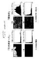
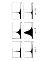
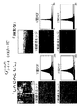
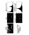
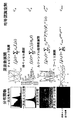
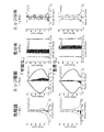
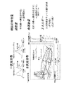
- the extremes of the aligned image group distribution Is an example showing the shape of the distribution function. It is a figure which shows the color histogram shape of the HVC surface of a "striking" image and a "mysterious" image. It is a figure which shows the distribution function of a color and a texture. It is a conceptual diagram of the higher order momentum space at the time of performing a Fourier transform. It is an image figure which shows the sensitivity group in a phase space. It is a figure explaining the relationship between a position and momentum and an uncertainty relationship.
- the texture PDF refers to a histogram of edge images. PDF is an abbreviation for Probability Density Function, and a high frequency band is extracted from an image, and its histogram is conventionally called PDF.
- texture PDF is not related to one existing high-frequency sub-band, but by integrating the high-frequency sub-band extracted with multi-resolution that was originally introduced in order to mimic a cognitive mechanism that makes visual judgment in an instant. It is a histogram of the obtained integrated edge image. In the histogram, the correlation of the spatial arrangement relationship of the contrast is reflected, and various shapes different from the generalized Gaussian function taken by the normal PDF shape of one high frequency band appear.
- the color histogram points out the importance of simultaneous description of the trend of the overall shape difference pattern in the combination of the V and C planes. Points out the importance of the difference in shape.
- the measure tentatively taken to extract the ambiguous shape was a statistic on the kurtosis and skewness of the V-plane and C-plane histograms in the case of color histograms.
- One important factor is whether it is possible to judge whether one of the VC planes has a two-band structure and one of them has a one-band structure, and the shape of the axis gradually changing between them. It was.
- the asymmetry of the histogram shape was evaluated using two indices, skewness and uniquely defined eviction.
- the evaluation of one characteristic in two dimensions by using two indices, the index sensitive to the base and the insensitive index shows the property of the duality. It also led to the consequence that it was important to get a connection with the adjectives that it had.
- the duality of adjectives is that the meaning of one adjective is divided into two major classification elements that distinguish the meaning between a major major classification element and the other adjectives contained in it. It means having both at the same time.
- kurtosis and skewness can be used to discuss the shape of asymmetry and kurtosis as parameters that represent deviations from the Gaussian distribution. Not prepared for. Therefore, unless the kurtosis, skewness, standard deviation, average value, etc. are used in combination, it is difficult to grasp the characteristics of the shape of the histogram and deal with the adjectives. Even if they are combined, for example, the kurtosis value does not have the ability to distinguish between two band structures and a uniform distribution structure. In addition, only a few adjectives can be explained.
- a sensitivity feature amount in the lowest layer in the lowest dimension there can be considered a scalar quantity-related element such as “representative hue, representative luminance, representative saturation” of a photographic image.
- a photograph is represented by the hue, brightness, and saturation with the largest area ratio, it is an overall “red” or “green” image, or an overall “under-exposed” “dark” image.
- HVC color distribution structure the vector quantity element related to color described by “HVC color distribution structure” is located. That is, when the HVC histogram is in a specific characteristic state, it is estimated that a slightly higher order sensitivity is evoked. Adjectives that fall under this hierarchy are considered to be “fresh” or “slow”, for example. An image having these impressions behaves strongly as a conspicuous sensibility prior to the previous low-order impression. However, the low-order impressions do not disappear and their properties remain. It is considered that the next feature is related to “edge, texture, contrast”. At the present time, it is estimated that the vector elements of the structure factor reduced one-dimensionally with respect to the texture correspond. Depending on the number of edges and textures and the strength of the contrast, it is thought that it gives an impression that the image is a “brilliant” image or a “rough” image.
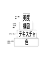
- composition that is, “spatial distribution” is located above. This is because “color” and “texture” described above can be discussed by extracting one-dimensional information from each color plane of HVC, but the spatial distribution must be discussed by extracting two-dimensional information from each plane. Then, it is considered that adjectives such as “noisy” and “dense” can be discriminated. It is thought that there is a structure like a universal aesthetic sense that is located above. However, it is presumed that it greatly affects the individual's sensitivity. It is estimated that an adjective such as “beautiful” can be discriminated from among them.
- the superiority of the obvious additive property is proved by the thought experiment in the case of the feature value of the non-additive property described later.
- the affective feature quantity must have an additive property as a description form that can reflect the hierarchy of adjectives in principal axis synthesis.
- Adjective ⁇ 1 F 1 + ⁇ 2 F 2 + ... + ⁇ 1 G 1 + ⁇ 2 G 2 + ... + ⁇ 1 H 1 + ⁇ 2 H 2 + ...
- a method for constructing a feature quantity having such an additive property will be specifically described below with respect to F i and G i in the following embodiments.
- the fact that the additive properties work well generates the same kind of invariants in each of hue, luminance, and saturation, and takes an arithmetic average among them. This also proves from the fact that more stable experimental results are born.
- the classification index has the following properties. For example, it is assumed that a certain feature amount has no similarity in color. At that time, even if the texture and the shape are similar, if the feature amount having no similarity acts and is placed at a distance away from the Euclidean distance, it can no longer be approached. That is, there is no superiority or inferiority relationship between feature amounts, and all are treated in the same row. Therefore, the higher-order feature quantity cannot overturn the result of the lower-order feature quantity. This property is therefore incompatible with the hierarchy of adjectives.
- the weight function that defines the orthogonality must be determined by selecting an optimal basis function according to the characteristics of the distribution function so as to be as close as possible to the human recognition process.
- Functions that are orthogonal by integration are generally called special functions, and many of them are defined by hypergeometric differential equations that are linear differential equations or confluent hypergeometric differential equations. Also, in order to be able to expand series, it must have completeness in the sense that the original function can be represented equivalently. Since the special function that forms such an orthogonal system does not necessarily have completeness, the special function that has both the selection function of the weight function and the completeness is limited.
- the first guideline for selection is the determination of whether the basis function group is similar to the shape of the distribution function currently targeted and the consistency of the interval region.
- Hypergeometric differential equation x (1-x) y "(x) + [c- (a + b + 1) x] y '(x) -aby (x) 0
- Confluent hypergeometric differential equation x y "(x) + [cx] y '(x) -ay (x) 0
- the description form of series expansion of the solution of the equation of motion satisfied by the state function by the function system having orthogonality and completeness is regarded as being the same as the expression in the Hilbert space.
- quantum mechanics the description of the equation of motion shifts to a matrix form by Hilbert space representation. Therefore, the construction of a Hilbert space requires expansion by a special function with complete orthogonality (see Document B1).
- the basis functions that make up the distribution function formulate one aspect of sensibility that at least the differential equation selected below is satisfied as the equation of motion. That is, it is considered that the hypergeometric differential equation is satisfied in the projection surface of the color distribution function and the confluent hypergeometric differential equation is satisfied in the projection surface of the texture distribution function.
- These linear differential equations are generic names of differential equation types and are located in different types.
- many inclusive types of differential equations can be derived by introducing parameter placement and variable transformation.
- a hypergeometric function that is a solution of a hypergeometric differential equation can handle a Chebyshev function, a Legendre function, or the like as a special case of parameters.
- confluent hypergeometric function that is the solution of the confluent hypergeometric differential equation leads to a Bessel function, a modified Bessel function, a Hermitian function, a Laguerre function, and the like as special cases. Furthermore, a spherical Bessel function and a spherical deformation Bessel function are derived by variable transformation of the Bessel differential equation (see Document B2).
- the Chebyshev function for the one-dimensional distribution function of the color and the spherical Bessel function for the one-dimensional distribution function of the texture. Therefore, if a sensuous differential equation exists in the brain, the linear differential equation is satisfied, and one of the projected surfaces of the color is a hypergeometric function describing the Chebyshev function, and another edge From the side of the confluent hypergeometric function that describes the spherical Bessel function, it can be said that the texture projection surface corresponds to the description on two different projection planes.
- the basis functions of the differential equations to be satisfied by the respective distribution functions play a role of simulating the coordinates of the wave type signal processing system called the brain by the Hilbert space.
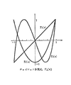
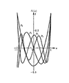
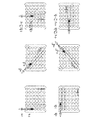
- FIG. 1 shows a graph of T 1 (x), T 2 (x), and T 3 (x) in the Chebyshev polynomial T n (x).
- T 1 (x) the exact orthogonal relationship including normalization conditions is given below.
- the orthogonality of the Chebyshev function places an extremely high density on the rising and falling parts of the distribution function. That is, when dealing with a function system that has a characteristic that suddenly occurs in a finite interval and ends suddenly like a histogram, the rising and falling parts are very important as the shape of the function. It shows that it cannot be approximated in a true sense unless it is accurately described.
- the spherical Bessel function can be described analytically.
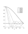
- FIG. 3 shows a graph of j 0 (x), j 1 (x), j 2 (x) of the spherical Bessel function.
- the orthogonality relation for the exact root including the normalization conditions is given below.
- the spherical Bessel function is a function having the maximum intensity at the origin in the case of a zero-order function, when the distribution function having the maximum frequency at the origin is approximated, the origin weight is always removed and the shape of the base is emphasized.
- various Bessel functions are functions suitable for description when light or waves diffuse from the origin toward the periphery, or when there is a singular point such as a light source at the origin.
- the spherical Bessel function is suitable for describing the wave of the radial component in the spherical coordinate system, and its strength decreases more rapidly as the distance from the origin is larger than that of the cylindrical coordinate system.
- the one-dimensional distribution function of the edge image to be handled now is close to the property of a spherical Bessel function because of its rapid intensity decrease rate.
- the spherical Bessel function always has a peak at the origin when a zero-order function is used, the weight of the origin is removed in order to evaluate the shape of the distribution function with the property that the peak always appears at the origin as in the histogram of the edge image. Therefore, focusing on the nature of the base is a very compatible method. As a result, it plays the role of creating a foundation that creates a linear relationship with the essence of the event.
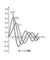
- the spherical Bessel function is a function that normally describes motion in the radial direction, it is usually defined in the positive region, but by expanding it to the negative region, Orthogonality also appears between functions of different orders. This is because the spherical Bessel function has the property that the even order is an even function and the odd order is an odd function.
- FIG. 4 shows a graph of spherical Bessel functions j 0 (x) to j 5 (x) defined to be enlarged in the negative region. Orthogonality of the order of spherical Bessel functions
- the positive region and the negative region of the distribution function can be developed simultaneously. Since root expansion always has completeness, it expands into a double series of orders and roots. For the time being, there is only one odd function for extracting the asymmetric component, so root expansion using two of the zeroth-order even function and the first-order odd function is sufficient.
- the expansion coefficient means that there are many components having a waveform and a frequency corresponding to the basis function in the distribution function.
- the expansion coefficient c i itself is suitable for the sensitivity feature quantity”.
- Dynamical system “Even if the motion state (momentum pi ) of each particle changes, there is a conserved amount (energy E) that characterizes the entire motion system.”
- Image system “Even if the pixel value distribution (state component c i ) of each image changes, there should be an invariant (I) that characterizes the sensitivity of the entire image.”
- the sum of the quadratic form of the expansion coefficient means that even if the distribution function changes variously, it is possible to extract the common features among the distribution functions of the image group that recall the same sensitivity.
- This summing operation alleviates the requirement for strict similarity between individual elements and aggregates a group of generally similar features, thereby deriving a function that collates features that are vaguely similar in shape.
- Kansei invariants must take the quadratic form is that the theoretical background in the process of deriving the equation of motion from the action function based on the principle of minimum action in theoretical physics and the process of building the Hamiltonian Is deeply involved. That is, assuming that one aspect of the kinematic field equation of motion satisfies the linear differential equation, the Lagrangian, which is the integrand of the action function, has a quadratic expression for the sensitivity field. Because it is required. This is because the equation of motion is derived based on the variational principle by putting the first derivative of the action integral equal to zero, and the superposition principle is maintained by dropping one order at that time.
- Integrating motion includes energy, momentum, and angular momentum, and it has been clarified by mechanics that these all have an important property of additiveity (see Document A2).
- the signal distribution of an image whose sensitivity is a problem is an image having a number of pixels on the order of 10 6 to 8 and a statistical group consisting of hundreds and thousands of images. It is necessary to use statistical physics.
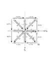
- n * n ground states ⁇ i ⁇ k represented by the direct product of a composite system are reducible expressions, and n (n + 1) / 2 symmetric products and n (n-1) It can be divided into two ground states represented by / 2 antisymmetric products (see Document A4).
- the characteristics of the shape of the distribution function in the same color plane are The shape of the distribution function between the color planes can be measured by the waveform expansion component created by the basis function, and the waveform expansion generated by the basis function of the antisymmetric product is combined with the waveform expansion component generated by the basis function of the symmetric product. It can also be measured by ingredients. Since the expansion components due to the waveforms of these synthesis systems are guaranteed to be orthogonal to each other in the ground state before synthesis, the expansion coefficients due to the ground state of the synthesis system are matrices in the form of symmetric products and antisymmetric products. It can be expressed as an element.
- Kansei invariants are defined by taking a matrix spur.
- spur usually refers only to the sum of diagonal elements, but here it is a new extended type that takes the diagonal sum of non-diagonal components with only a constant quantum number difference between the row and column positions.
- a spur the ratio of the components of the composite waveform of the two ground states that maintain a constant quantum number difference in the distribution function can be summed over all the composite waveforms that can be created. It can be detected in the taken state. Between two distribution functions with different color planes, the proportion of combinations of different ground states with a certain quantum number is present in two proportions: symmetric state and antisymmetric state of the combination. It is evaluated with the composite waveform.
- the sensitivity invariant defined above will be compared with the field invariant in the electromagnetic field.
- the document A5 there are two types of invariants for the Lorentz transformation of the electric field E and the magnetic field H: a true scalar and a pseudoscalar.
- a sensitivity invariant that gives the same sensitivity even when moving from one image to another has a configuration very similar to the field invariant when converted from one reference system to another reference system in an electromagnetic field.
- sensitivity invariants corresponding to kinetic energy, but there are more than two types of “sensitivity fields”, and it is more straightforward to think that field energy is transmitted. is there.
- the components of the electromagnetic field are four-dimensional in time and space, but it is presumed that there are at least elements of the order necessary for describing the distribution function in the sensitivity component.
- an electric signal circuit induced in the field is constructed against these sensitive fields, or the neural circuit that is excited instantaneously in energy. It is a natural idea to acquire energy levels.
- FIG. 5 is a block diagram illustrating an image classification apparatus according to the embodiment.
- the image classification device is realized by the personal computer 10.
- the personal computer 10 is connected to a digital camera or other computer, receives image data from the digital camera or other computer, or receives image data from a memory card installed in a memory card slot, and receives a hard disk device ( (Not shown).
- the personal computer 10 performs image classification processing described below on the stored image data.
- the loading of the image classification program into the personal computer 10 may be performed from a storage medium such as a CD-ROM storing the program, or may be performed via the network 12 or the like.
- the program read from the hard disk device 16 connected to the server 14 is loaded.
- the personal computer 10 includes a CPU and peripheral circuits controlled by the CPU, and performs image classification processing shown in the flowchart of FIG. 6 based on a program in which the CPU is installed.
- Conversion to Munsell HVC color space (step S1 in FIG. 6)
- the input image is converted into a Munsell color space with high human perceptual color uniformity.
- the Munsell color space is a color space that is divided so that the hue H is divided by 100 degrees around the circle, the luminance V is distributed between 0 and 10, and the saturation C is distributed between 0 and 25.
- This is a color space designed so as to satisfy an equal rate of perceiving C color difference 2 as 1 as an equivalent color difference.
- the region where the C value is 1 or less, the V value is 0.5 or less, and the region where 9.5 or more is defined as N (neutral hue).
- the input image is, for example, an image expressed in an sRGB color space with an output gamma characteristic
- it is first converted to a linear gradation and then converted into an XYZ space according to the sRGB standard.
- a hue surface is prepared as an N (neutral) separation surface.
- step S2 in FIG. 6 Create a histogram for each HVC plane.
- the number of bins in the histogram should be set to about 200 for all of H, V, and C.
- the hue surface is a surface on which N separation is performed. Therefore, the area ratio classified into N is not included in the histogram of the H plane even if it is integrated with the hue circle.
- N is distributed randomly in the hue circle, so a random and uniform offset distribution is excluded from the histogram of the hue plane, and the original chromatic color histogram shape remains.
- the histogram value is normalized by the number of pixels, a one-dimensional distribution function representing the probability density of the pixel value is obtained.
- the distribution function schematically created is expressed as follows.
- f (H), f (V), f (C) 3. Hilbert space representation of distribution function (step S3 in FIG. 6) 3-1.
- Variable transformation If the horizontal axis of the histogram is [a, b] and the vertical axis is [fa, fb], the horizontal axis is [-1,1] and the vertical axis is [-1,1].
- Variable conversion is performed in the interval that fits in. For convenience only in this section, if the variable on the horizontal axis is converted from x to y and the variable on the vertical axis is converted from fx to fy, the conversion formula is as follows.
- the constant factor in the series expansion coefficient shown below is added depending on the definition of variable transformation on the vertical axis. Assuming that the expansion coefficient corresponds to the momentum as explained in the introduction, the constant factor remaining by the statistical average of the image group depends on how the Hilbert space coordinate system of the entire image group is selected. It is equivalent to remaining as a translational movement.
- the expansion coefficient c n is obtained by the following equation using the orthogonality of the basis functions.
- variable conversion is introduced.
- Step S4 in FIG. 6 The shape of the distribution function of the H, V, C histogram is extracted by a synthesis system of two Chebyshev basis functions. That is, the sensibilities that appear due to the structure taken by the HVC distribution function are extracted as feature quantities.
- ⁇ ⁇ ⁇ ⁇ Kansei invariants are defined by spurs of matrix elements having a certain quantum number difference for matrix elements created by the quadratic form of expansion coefficients.
- An example of creating quantum numbers up to 0, 1, 2 is shown.
- it is standardized and defined so that all invariant values fall within [-1,1].
- An invariant with a plus sign indicates the proportion of the waveform that is signed due to the symmetry of the composite system in the distribution function of the image, and an invariant with a minus sign is in the distribution function of the image. It shows the existence ratio of the waveform with the sign due to the antisymmetric state of the synthetic system.
- the value of the invariant is close to zero, it means that there is no component of the composite waveform, and if it is close to +1, it means that there are many components in the form of the composite waveform. If it is close to 1, it means that there are many components of the waveform obtained by inverting the sign of the composite waveform.
- the symmetric state and the antisymmetric state are conjugated with each other.
- the sensitivity invariants of the symmetric product and antisymmetric product of the same quantum number difference when examining the degree of alignment of the image group related to the invariant, it is unclear what sensitivity is gathered near zero in the symmetric product.
- a group of images appears at both ends of the index distribution in the antisymmetric product.
- an image group that is unknown in the anti-symmetric product index appears at both ends of the image distribution in the symmetric product index. This fact is a natural consequence of the following mathematical formula.
- step S5 in FIG. 6 Linear combination of Kansei invariants Creates a new index Q i that linearly combines Kansei invariants using the additive property of Kansei invariants as an index for searching for Kansei adjectives (i) .
- the adjectives that can be represented by the index Q i are not only one adjective but also a pair of adjectives that have adjectives of the opposite nature.
- Q i ⁇ 1 F 1 + ⁇ 2 F 2 + ...
- the value of the linear coupling parameter ⁇ i is normalized so that Q i becomes an index in the range of [ ⁇ 1, 1] again.
- Parameter setting for search target adjectives Linear combination parameters corresponding to predetermined adjectives are learned in advance, and the model parameters are set.
- Image classification process (step S6 in FIG. 6) The images are classified based on the adjective discrimination index. For each image in the image database group to be input, an adjective discrimination index Q i is calculated and rearranged in order of the value of Q i .
- the frequency distribution of the image group with respect to the discriminant index Q i is shaped like a Gaussian distribution or Poisson distribution, so it is unique to the adjective discrimination index at a level that is statistically significant at the both ends. An image showing sex is presented.
- the range of effective quantum number difference is that when the non-diagonal component of the matrix element is smaller than the value that the diagonal component can take, that is, when it is relatively smaller than ⁇ 1, there is no longer a meaningful sensitivity classification ability. It is appropriate to think of it not. That is, when the distribution range of the values of the sensitivity invariant, which is a spur of the matrix elements, is wide, alignment with high correspondence with sensitivity can be obtained, but when the distribution range becomes small, the correspondence relationship can no longer be seen. This has been confirmed experimentally.
- FIG. 8 shows an example of the color histogram shape of the HVC plane of an image located near both ends of the image distribution.
- the color histogram of a “static” image is collective with a shape like one band structure in which all of the H, V, and C planes are collected in one basis function state component.
- a “dynamic” image has many complex peak shapes on each of the H, V, and C planes, and has a histogram structure that is unlikely to be described with a simple waveform and is dispersive.
- the sensitivity images of the adjective pair “tightened-open” are aligned.
- images having many shadows are collected.
- a lot of images with a little brightness and spatial extent are gathered in the “open” image as a whole.
- FIG. 9 shows an example of the color histogram shape of the HVC plane of an image located near both ends of the image distribution.
- the color histogram of the “tight” image is very similar in shape between VCs.
- the color histogram of the “open” image has completely different shapes on the V and C planes.
- This sensitivity invariant aligns the sensitivity images of the adjective pair “excited-sedated”.
- This adjective pair is positioned in a conjugate relationship with the “tight-open” adjective pair derived from the symmetric product.
- “Excited” images include fancy gingko and maple trees and leaves, or a photo that captures the pink glow of a moment in the evening of a landscape photo and a moment when clouds appear. Many photographs that capture the movement of On the other hand, the “calm” image captures the moment when the movement is completely stopped and collects photographs with deeper colors.
- ⁇ Model learning of sensitivity adjectives> The value of the sensitivity invariant is uniquely determined from the observed amount of the distribution function of the image. It is necessary to determine a linear combination parameter for each adjective in order to obtain a correspondence with the adjective by pre-learning.
- Least square method For one or more adjectives, an image having the impression is selected from a group of images for learning data. A square error function for measuring the reproducibility of the parameters is introduced, and each coupling parameter is determined in such a manner that each parameter is partially differentiated to find a minimum point, assuming that the linear coupling parameter is unknown. This is a coefficient fitting by the least square method.
- the coordinate position obtained by simply statistically averaging the selected image group within each sensibility invariant gamut is used as the adjective.
- the learning result of the linear combination parameter for If a group of images selected for a given sensitivity invariant is scattered, the value of the parameter ⁇ i approaches zero by statistical averaging, which means that the sensitivity invariant is irrelevant for the adjective.
- the selected images are gathered in the same direction, even if statistical averaging is performed, a significant value remains in the parameter ⁇ i , and the sensitivity invariant is important for the adjective. In this way, a sensibility invariant that works specially for an adjective can be derived very simply.
- the model learning method described above can be commonly used in all the embodiments described below.
- the method of taking the one-dimensional coordinates in the hue circle may be to make the red that is the origin of the Munsell hue circle around the starting point, and to make the end point red magenta again, but more preferably as in the first embodiment. It is preferable to cut a point where the hue distribution frequency is minimum in each image and set a start point and an end point there. This is because the signal intensity fluctuates at both ends due to the division of the hue ring, and adverse effects due to overestimation of edge components when edges are extracted within the color plane are minimized.
- edge image 2-1 Multi-resolution transformation and edge extraction
- Wavelet transformation The wavelet transformation is used to project a high-frequency edge component of each color plane of HVC by projecting to the frequency space expressed in multi-resolution.
- LH, HL, and HH the wavelet-decomposed high-frequency subbands LH, HL, and HH are used as they are as edge components. If you write this state schematically, when disassembling to resolution M stages It becomes. Since the LL component is sequentially decomposed into high-frequency subbands with low resolution, the only remaining LL component is the lowest resolution. For example, the following 5/3 filter is used as the wavelet transform.
- the one-dimensional wavelet transform defined above is subjected to wavelet decomposition by performing two-dimensional separation filter processing independently in the horizontal and vertical directions.
- the coefficient s is collected on the L plane, and the coefficient d is collected on the H plane.
- Laplacian pyramid In addition to wavelet transform, there is another method of multiresolution conversion that uses a Laplacian pyramid.
- a Laplacian pyramid once create a reduced image (vertical / horizontal) * (1/2), restore it to the original size by bilinear scaling, and take the difference from the image before reduction.
- a high-frequency image Laplacian component
- smoothing for preventing aliasing may be performed before a reduced image is created. If this is repeated one after another, a Laplacian pyramid with a series of high-frequency images is formed. As with the wavelet transform, only one low frequency image (Gaussian component) remains at the lowest resolution.
- Document D1 describes that a histogram of high-frequency band signal values generated by multi-resolution conversion in this manner (called a probability density function, abbreviated as PDF) has a Gaussian distribution or a Laplace distribution.
- PDF distribution can be approximated by symmetrical Generalized Gaussian.
- the value of the multi-resolution conversion stage number M may be decomposed to a point where the PDF histogram of each band has a pixel number that is not rough. For example, it may be about 5 stages for Quad VGA size (1280x960) images, about 3 stages for QVGA size (320x240) images, and about 7 stages for 20 million pixel images.
- FIG. 10 is a diagram showing a state of subband division by four-stage wavelet transform.
- high-pass component data and low-pass component data are first extracted from all rows in the horizontal direction with respect to real space image data.
- the data of the high-pass component and the low-pass component with half the number of images in the horizontal direction are extracted.
- the high-pass component is stored on the right side of the memory area where the real-space image data was stored, and the low-pass component is stored on the left side.
- high-pass component data and low-pass component data are extracted for all columns in the vertical direction.
- data of a high-pass component and a low-pass component are further extracted from each of the high-pass component on the right side of the memory area and the low-pass component on the left side.
- the high-pass component and the low-pass component are stored in the lower side and the upper side of the memory area where the respective data exist.
- the data extracted as the high-pass component in the vertical direction from the data extracted as the high-pass component in the horizontal direction is represented as HH
- the data extracted as the low-pass component in the vertical direction from the data extracted as the high-pass component in the horizontal direction Is represented as HL
- data extracted as a high-pass component in the vertical direction from data extracted as a low-pass component in the horizontal direction is represented as LH
- the data is denoted as LL.
- the vertical direction and the horizontal direction are independent, it is equivalent even if the order of extraction is changed.
- the high-pass component and the low-pass component are similarly applied to the data LL extracted as the low-pass component in the vertical direction from the data extracted as the low-pass component in the horizontal direction in the first-stage wavelet transform. Perform extraction. If this is repeated up to four stages, the result is as shown in FIG.
- PDF is a histogram of edge strength, it has a distribution with the peak at the origin with the same degree of positive and negative frequency integration area.
- a symmetric PDF distribution shape in each layer is integrated into a symmetric PDF distribution shape as it is.
- the state of the correlation can be projected in the form of a PDF distribution shape.
- a one-dimensional distribution function representing the probability density of the pixel value is obtained.
- the distribution function schematically created is expressed as follows.
- the Laplacian symbol ⁇ is used because the integrated edge image describes the secondary differential aspect of the pixel value of the original image.
- Hilbert space representation of distribution function The distribution function of the integrated edge image is series-expanded with a spherical Bessel function, and the shape can be evaluated by the expansion coefficient.
- right development and left development are performed separately, but in the third embodiment described later, left and right simultaneous development is performed.
- Variable transformation For the portion on the right side of the peak of the histogram, the distribution area on the horizontal axis is [a, b] (a ⁇ b), and the distribution area on the vertical axis is [fa, fb]. Variable conversion is performed in the interval where the horizontal axis is in [0,1] and the vertical axis is in [0,1]. Similarly, the left side of the histogram peak is set to [b, a] (b ⁇ a) on the horizontal axis and [fa, fb] on the vertical axis, and the same conversion is performed. Usually takes values a to 0 and fa to 0.
- variable on the horizontal axis is converted from x to y and the variable on the vertical axis is converted from fx to fy
- the conversion formula is as follows.
- Variable transformation on the horizontal axis: y
- Variable conversion on the vertical axis: fy (fx-fa) / (fb-fa) 4-2.
- Series expansion by the root of the spherical Bessel function The distribution range of the horizontal axis subjected to the above-described variable transformation is represented by x regardless of ⁇ H, ⁇ V, and ⁇ C.
- each HVC color plane is expanded with a basis function based on the roots of N zeroth-order spherical Bessel functions.
- the meaning of the symbol a used here is different from the above, and means the outermost contour point that is the target of development of the distribution area.
- the expansion coefficient c n is obtained by the following equation using the orthogonality of the basis functions.
- ⁇ nm means the value of the mth zero of the nth order function.
- the root of the zeroth order function can be given analytically.
- the spherical Bessel function is a complete system with respect to root expansion, the original function can be completely reproduced by taking a sufficiently large value of N.
- the method of creating a quadratic invariant is more than that of the first embodiment.
- the number of types increases more than twice.
- the following shows an example of how to create an invariant when the quantum difference is 0 and 1 in the case of a symmetric product, and how to make an invariant when the difference is 1 in the case of an antisymmetric product.
- a composite system can be created in the same way as in the first embodiment from the combination of two basis functions in the same quadrant on the HVC3 plane, and between different quadrants.
- a composite system can also be created from a combination of two basis functions. Since the former handles only the radial direction, the symbol “r” is given. The latter gives the symbol “z” in the sense that it crosses zero.
- the expansion coefficient on the right be c k ( ⁇ +) and the expansion coefficient on the left be c k ( ⁇ ) .
- it is standardized and defined so that all invariant values fall within [-1,1].
- Image Classification Processing Based on the adjective discrimination index, images are classified as in the first embodiment. In the following, a specific example is given to show what kind of sensibility is actually given. Similarly to the first embodiment, in the case of texture, from each sensitivity invariant, it was possible to obtain an image alignment having a very deep relationship and linearity with high-order adjective pairs used in color psychology.
- the situation is slightly different from that of the color distribution function of the first embodiment.
- the edge distribution function a large value remains even when the element of the off-diagonal component is away from the diagonal region, and the former is Compared to the short-range correlation whose strength decreases rapidly when leaving the angular range, it has a long-range correlation property. This can be interpreted as indicating that the number of emotions induced by the texture distribution structure is greater than the number of emotions induced by the color distribution structure.
- This sensitivity invariant aligns the sensitivity images that are the combination of two adjective pairs, “lively-lonely” and “gorgeous-clean”. “Buzzy, gorgeous” images are a collection of images of various scenes that include many large and small structures. On the other hand, the “lonely, neat” image contains many photographs that contain dark-colored structures and dark shaded scenes with an area specific gravity that has some visual influence.
- the sensitivity images of the adjective pair “Smudged-Mysterious” are aligned. Many images with trees and shades are gathered in the “smeared” image.
- the "mysterious” image is accompanied by a picture of a large area, a section of landscape, a dyed pink, orange, yellow, etc. at dusk, or a series of strange clouds. Many images like steam and haze are collected.
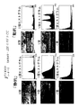
- FIG. 12 shows a typical edge image and distribution function of images selected at both ends.
- the V plane and the C plane both have a lot of edges and textures, giving a familiar impression.
- the distribution function of the V-plane edge image shows a strong value with a slight frequency, that is, if there is a small base in the distribution function, the original picture is divided into sections such as mountain ridges. It is considered that a ghostly impression is given by the fact that the change of the saturation plane is woven with a thick contrast width larger than the contrast change of the luminance component.
- Hilbert Space Representation of Distribution Function A distribution function is represented in Hilbert space by a double series of root expansion by a zero-order spherical Bessel function that is an even function and a root expansion by a first-order spherical Bessel function that is an odd function. Then, all the symmetric components of the distribution function shape are collected in the expansion coefficient of the zero-order function, and all the asymmetric components are collected in the expansion coefficient of the linear function. Further, the double series may be expanded to an infinite order by further development.
- Variable transformation Let r be the distance from the peak position p of the histogram to the extreme end of the distribution area that extends to the farthest right or left.
- the distribution range on the horizontal axis is [-r + p, r + p].
- Variable transformation is performed on the horizontal axis in the interval [-1,1].
- Variable transformation on the horizontal axis: y (xp) / r
- the vertical axis is the same as in the second embodiment.
- the expansion coefficient c nk is obtained by the following equation using the orthogonality of the basis functions.
- the product of the zero-order and first-order function since the internal variable is an odd function be how scaled, and further consideration of the even function of [rho 2, left and right
- the relational expression of the orthogonality regarding the order is not limited to the case where the weighting function is 1 as long as it is defined between the even-order function and the odd-order function, and can be applied even if the weight of an arbitrary even function is added.
- the constant factor of normalization will vary but, (described in the portion of the outline description) that already have been given by the equation according to the roots in the case of [rho 2.
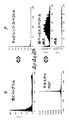
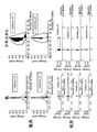
- FIG. 13 is a diagram illustrating a distribution function of color and texture. As described so far, the sensitivity of the image and the shape of the distribution function are very related, and the shape similar to the ambiguity tends to give the same sensitivity. Physical techniques have been introduced to quantify the shape recognition of this distribution function.
- Quantum mechanical method The contents explained so far are to try to describe by quantum mechanics. That is, it can be summarized as follows. 1) The distribution function f is projected onto the Hilbert space and the momentum p is displayed. 2) constructing an additive energy E n of the quadratic form with group theory. The method adopted here actually introduces the concept of quantum mechanics, and describes the state of a multi-system with a large number of pixels and a large number of gradations as a statistical mechanics through a distribution function f. Also included. This will be described in detail below.
- Image signal S (x, y) Sub system information f (p, q) Energy information ⁇ 10 ⁇ 23 pcs Color: (256) ⁇ 3-10 ⁇ 7 ⁇ 2000 pcs Texture: ( ⁇ 256) ⁇ 3-10 ⁇ 8-2000 Composition: Number of pixels-10 ⁇ 7 (-2000)
- the variables p and q are symbols that represent the independent variables p1, p2, ..., pi, ..., q1, q2, ..., qi, ... Used as
- a quantum mechanical description based on an incomplete set of data about a system is done using a density matrix.
- the expected value of any physical quantity can be calculated using the density matrix.
- ⁇ ⁇ n c n ⁇ n
- Substituting this into the expression of the density matrix gives the density matrix in energy display: c m * c n ⁇ w mn Can guide you.
- the diagonal component of the energy display density matrix represents a steady state.
- One off-diagonal component represents an unsteady state.
- Statistic average also calculates expected value in steady state.
- the sensitivity of the image is not limited to the steady state, and the non-steady state needs to be considered. Therefore, it is necessary to calculate the expected value in consideration of both the steady state and the unsteady state.
- the steady state is defined as one energy level state (E 0 ) by taking the diagonal sum of all steady states.
- the unsteady state is described by the energy level (E n ) of how far away from the steady state to the unsteady state by taking the diagonal sum of the non-diagonal components. Take the way.
- the image variables corresponding to the position coordinates q and the momentum p, which are mechanical variables, are defined differently for each sub-system.
- the color represents the distribution of signal values with an interval width of "zero to positive finite value” and describes the distribution of the original signal itself. Therefore, a function that satisfies the linear differential equation suitable for the description is a hypergeometric function. Any function included.
- the texture represents the distribution of the signal value with the interval width from “negative finite value to positive finite value” from which the edge component is extracted, and describes the distribution of another aspect from which the original signal information is dropped.
- the function satisfying the linear differential equation suitable for description is any function included in the confluent hypergeometric function. Since the composition represents a two-dimensional distribution of signal values with an interval width of “zero to positive finite value” and describes the distribution of the original signal itself, the function satisfying the linear differential equation suitable for the description is Any function included in the hypergeometric function.
- the hypergeometric function represented by a differential equation having three singular points is suitable for representing the distribution of the signal value of the image itself, and the image signal that comes to the argument of the distribution function is zero as the pixel value. It is suitable for describing the property that an image signal composed of the above values can be uniformly distributed.
- the confluent hypergeometric function expressed by a differential equation having two singularities in total by merging the two singularities into one has the aspect of reducing the amount of information about the signal value of the image by one. Suitable for description, as an image signal that comes to the argument of the distribution function, an image signal that spans positive and negative values, such as an edge signal value from which one piece of information has been dropped by differentiation, is localized near zero. Suitable for describing properties to be
- the hypergeometric function suitable for describing the one-dimensional color distribution function is the Chebyshev function. Since this function forms a complete system with a single series of even and odd functions, the even function is angular momentum 0 and the odd function is angular. If it is regarded as momentum 1, it can be considered that the spin coordinates of spin 1, which is the same Bose particle as light, are described. Therefore, it can be considered that the one-dimensional distribution function of color describes a wave function of a spin system among the wave functions.
- the confluent hypergeometric function suitable for describing the one-dimensional distribution function of the texture is a spherical Bessel function.
- the spherical Bessel function is the only function that can be expanded and defined in the negative region of the Bessel function. Therefore, it can be understood that the one-dimensional distribution function of the texture describes the radial wave function among the wave functions. Since the radial wavefunction can be described by a double series of two series related to the order and root of the even and odd functions, the angular momentum 0, 1, 2, 3, ... They can be mapped to what are called s, p, d, f, ... orbitals in atomic orbitals.
- the hypergeometric function suitable for the description of the two-dimensional distribution function of the composition is considered to be a Legendre function or a spherical harmonic function that is a product of the Fourier function with the Legendre function. Therefore, it can be considered that the two-dimensional distribution function of the composition describes a wave function corresponding to the two-dimensional system coordinates of the zenith angle and the azimuth in the spherical coordinate display.
- the statistical average for deriving the statistical properties of the image system has two meanings. That is, one point is that a huge amount of information on color, texture, and composition is reduced to a macroscopic physical quantity by a statistical average. Another point is that a definite value is obtained by taking an average of image groups in the sense that a large number of model image groups have a common sensitivity.
- the former includes a quantum mechanical average operation and a statistical average operation at the same time, accompanied by a conversion process from a microscopic physical quantity to a macroscopic physical quantity.
- the latter is mainly regarded as including a statistical averaging operation for determining a statistical property by determining an amount corresponding to an average value of fluctuations of a macroscopic physical quantity. Therefore, the former makes a signal that makes a macroscopic action on the brain through the visual system, and the latter plays a role of knowing the average element of the distribution of actions in the brain of the sensation received by a person.
- the momentum and angular momentum of a closed system are related to the uniform translational motion and uniform rotational motion of the entire system. It does not describe the statistical properties of the system. However, it is meaningful in the sense to distinguish it from the uniform translational motion and rotational motion of other images. That is, if a coordinate system in which the translational and rotational motions of a closed system of a single image are stationary is taken, only the energy determines the statistical properties of the single image, but the coordinate system common to other images Since the momentum and the angular momentum are different from those of the image group, they are recognized as different images. However, when describing the macroscopic properties common to many images, that is, sensibility, the momentum and angular momentum are information that disappears to zero or a constant value when the statistical average of the image group increases.
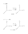
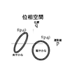
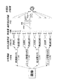
- FIG. 15 is a pictorial diagram showing the sensitivity group in the phase space.
- Sensitivity description is also a question of how to describe ambiguity quantitatively.
- the locus of the phase space where the distribution function satisfies a certain condition describes the state distribution that evokes the same sensitivity.
- the constant condition represents a trajectory on the phase space that satisfies a condition in which energy, which is a mechanical invariant, is constrained to a constant value.
- the ambiguity of sensibility is described as a collection in which the distribution function can take various states as an image, but they are all on the locus of a blurred range in the same phase space.
- the logarithm of the distribution function is an integral of motion, which is a mechanical invariant, and is described by an integral of additive motion.
- the distribution function of a composite system which represents the probability that the distribution function of one subsystem and the distribution function of another subsystem simultaneously take that state, is represented by the product of the distribution functions of the subsystem, and its logarithm is an additive property. Because it has.
- the momentum and angular momentum which are other mechanical invariants, play a role as additional constraints for that purpose, and in addition to energy, the trajectories on the phase space satisfying the constant momentum and angular momentum respectively.
- the distribution range exerts a sensibility effect common to a small number of model images. As a limit of the minority model, a similar image search of a single image is applicable.
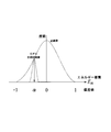
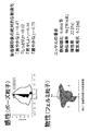
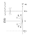
- FIG. 16 is a diagram for explaining a situation in which the relationship between the position and the momentum satisfies the uncertainty principle in the projection onto the high-order space regarding the color and texture of the image system. That is, as in the case of the texture PDF illustrated in FIG. 16, when a sharp peak is raised with respect to the position and the accuracy of position coordinates is high, any frequency can be obtained by trying to realize the waveform in a momentum space obtained by spherical Bessel-Fourier transform. Since it cannot be achieved without overlapping a large number of momentums, the momentum becomes uncertain and has a very wide distribution.
- the value of the plank constant h is related to the concept of a histogram bin that defines the gradation width with respect to quantization in the gradation direction and one pixel that defines the pixel interval with respect to quantization in the spatial direction. . Therefore, when the number of gradations of an image system is reduced or a reduced image is generated, the Planck constant value needs to be changed according to the quantization method of the system, and changes depending on the situation to be considered. This is different from the situation where the entire system can be treated as a constant regardless of the subsystem, such as physical constants. However, the Planck's constant in the image system can be treated as a fixed value in a sub-system in which a certain width is projected and the quantization width is defined.
- the kind of substance is composed of 118 kinds of elements, their compounds, alloys, etc. as a simple substance, and exists in the order of thousands to 10,000. For example, when the number of combinations of 2 to 3 elements out of 118 elements is calculated, this number is obtained.
- the number of elements and the basis of their properties are defined by the radial wave functions s, p, d, f orbits that can exist as atomic orbitals and the degenerate numbers of those states.
- Such dihedral properties are also present in the properties of materials.
- the wave function in the radial direction is s orbital and p orbital in the upper direction in the vertical axis direction.
- Different things are lined up.
- elements present in the same row in the vertical direction exhibit chemically very similar properties, and exhibit similar properties when present adjacent in the horizontal direction.
- the energy level in the low-order subspace is the discrete energy level, which is the field energy created by the mean field approximation of statistical physics. That is, construct a discrete scalar invariant.
- the energy level in the higher-order subspace is considered as a continuous energy level in the process of gradually separating from the stationary state of the diagonal component of the energy matrix to the unsteady state of the non-diagonal component. That is, construct a continuous vector invariant.
- the momentum distribution has a highly variable characteristic that varies very randomly depending on the image, and even if a statistical average is taken for a group of images with the same sensitivity, a common factor Almost no elements remain.
- a factor that acts in common in an image group having the same sensitivity tends to remain.
- an image that is “killing scenery” has a high probability that the average luminance ⁇ V> and the average saturation ⁇ C> have a small value at the same time, and the kinetic energy ⁇ V> ⁇ C> shows a small value in common.
- the average luminance ⁇ V> and the average saturation ⁇ C> have a small value at the same time
- the kinetic energy ⁇ V> ⁇ C> shows a small value in common.
- the value of ⁇ V> may be larger, in which case ⁇ C> is balanced by showing a smaller value.
- ⁇ V> and ⁇ C> are taken separately, the average of the momentum tends to disappear as information in the average value of the general image. This is shown below.
- Momentum p energy E n Hue H Statistical average ⁇ V> ⁇ C> Luminance V ⁇ ⁇ V> ⁇ V> Saturation C Residual information ⁇ H> ⁇ V ⁇ C ⁇ C ... (Random distribution) (Simultaneous alignment) 1)
- Momentum Examples of the momentum element pn include the following. ⁇ H>, ⁇ V>, ⁇ C>, ⁇ H , ⁇ V , ⁇ C Note that the portion of ⁇ may be treated as an element M n of angular momentum.
- the elements E n of Energy Energy include the following. Energy elements E n, because different energy elements are calculated, will be represented their state ellipsize the following as a symbol for distinguishing them.
- the symbol a is used for the ⁇ plane, b for the ⁇ plane, m for the average value, and s for the standard deviation value.
- 21 + 5 26 types of scalar invariants are derived as energy elements of low-order invariants of color. These are each correspond to discrete energy levels E n, represents the value itself of E n. This is a macroscopic physical quantity that has been reduced in the lower-order subsystem of the color.
- ⁇ H> is expressed as a complex number and separated into two components to realize the description. Moreover, the ratio which subtracted the neutral part which remains in the hue ring by the magnitude
- size of the absolute value of a complex number at that time is represented. ⁇ H> (1-pop (N)) exp (2 ⁇ i ⁇ H ( ⁇ N)> / 100) ⁇ H calculates the spread width of only the distribution function in the hue circle. Therefore, it remains one component. This strength is also evaluated by multiplying the frequency ratio remaining in the hue ring in conjunction with the absolute value of ⁇ H>. That is, when all flow into neutral, ⁇ H is always defined to be zero.
- ⁇ H (1-pop (N)) ⁇ H ( ⁇ N) ⁇ Lower-order invariants of texture>
- the edge surface representing the texture the integrated edge surface described in the second embodiment, in which each Munsell HVC surface is subjected to multi-resolution conversion and only high-frequency subband images are integrated by inverse conversion, is used.
- the edge strength of the edge surface is schematically expressed as ⁇ H, ⁇ V, ⁇ C using a Laplacian symbol ⁇ .
- the values of the edge strengths ⁇ H, ⁇ V, and ⁇ C of the HVC surface represent the momentum.
- the average value and the standard deviation value of the momentum are obtained from the distribution function f (p) representing the momentum distribution. That is, it is obtained from the histograms f ( ⁇ H), f ( ⁇ V), f ( ⁇ C) of the edge intensity of ⁇ H, ⁇ V, ⁇ C.
- the low-order invariant of the texture is obtained by the same procedure as that for the low-order invariant of color.
- 1) Momentum Examples of the momentum element pn include the following. ⁇ H>, ⁇ V>, ⁇ C>, ⁇ ⁇ H , ⁇ ⁇ V , ⁇ ⁇ C Note that the portion of ⁇ may be treated as an element M n of angular momentum.
- the elements E n of Energy Energy include the following. Energy elements E n, because different energy elements are calculated, will be represented their state ellipsize the following as a symbol for distinguishing them.
- the symbol a is used for the ⁇ plane, b for the ⁇ plane, m for the average value, and s for the standard deviation value.
- the edge component of the hue plane shall take the edge of the color plane displayed with a value where the Munsell value is always 0 as the origin of the hue circle. This is because, rather than experimentally changing the cut point of the hue ring to a point where the distribution function is minimized for each image, it is better to observe the hue plane in a fixed manner at the origin of the same Munsell value as the iridescent spectrum distribution This is because it has been found that the edge is preferable. Further, neutral is not treated separately, but is a hue plane distributed at any point of the hue circle. Therefore, the neutral component behaves like random noise on the hue plane.
- ⁇ Higher-order invariants of color The Chebyshev expansion of the color distribution function.
- the variable x takes each value of H, V, and C.
- f ( ⁇ x) obtained by inverting the axis of the distribution function f (x) is also added to the consideration.
- the physical meaning of axis inversion corresponds to gradation inversion.
- the concept of angular momentum is introduced. That is, the basis function group is divided into subgroups according to the difference in properties between the even function and the odd function, and an angular momentum quantum number is assigned to each subgroup.
- the basis functions of odd-numbered angular momentum quantum numbers are inverted in sign, and the basis functions of even-numbered angular momentum quantum numbers are unchanged.
- parity in quantum mechanics Such a property relating to the axis inversion of the wave function of the angular momentum unit is called parity in quantum mechanics.
- Even-function basis functions have even parity and are invariant to axis inversion, and odd-function basis functions have odd parity and invert the sign with respect to axis inversion.
- this angular momentum quantum number describes a spin system
- the Chebyshev function is defined only by a single series expansion, the even function and the odd function describe the states of spin 0 and spin 1, respectively, and a state in which the parity of the state of spin 1 is inverted by axis inversion can be generated.
- the Chebyshev function is suitable for describing a spin-1 system that is a Bose particle.
- the momentum element p n the angular momentum element M n , and the energy element E n when the axis of the angular momentum describing the system is not reversed are constructed, and then each of them is constructed.
- the element of about twice the angular momentum inversion is derived.
- the linear combination coefficient is derived from the viewpoint of describing a meaningful independent component. That is, when only the sign of the element changes, it does not make sense because the same system is described if the sign of the linear combination coefficient is changed.
- momentum falls into this category, but angular momentum and energy can be derived as separate components.
- the linear sum of the expansion coefficient of the odd function can be a macroscopic index for evaluating the asymmetry of the distribution function.
- M rxp
- the above definition takes the product in a coordinate space with the angular momentum quantum number of the Hilbert space coordinates as the distance from the origin for the partial sum of the momentum.
- 1x3 3.
- an energy matrix (i, k) of a symmetric product and an antisymmetric product can be constructed from the product of the ( ⁇ ) plane and the ( ⁇ ) plane.
- c i ( ⁇ ) c k ( ⁇ ) + c k ( ⁇ ) c i ( ⁇ ) c k ( ⁇ ) -c k ( ⁇ ) c i ( ⁇ ) Each of these is a square matrix arranged vertically and horizontally by the number of basis functions.
- a diagonal sum that is, a spur is taken.
- the number of elements to be spured must be defined to be the same as the number of elements in the diagonal sum, and the basis functions used in one of the products must lick all the basis functions that make up the complete system once. Build in shape.
- an energy matrix (i, k) of a symmetric product and an antisymmetric product can be constructed from the product of the ( ⁇ ) plane and the ( ⁇ ) plane.
- an energy matrix (i, k) of a symmetric product and an antisymmetric product can be constructed from the product of the ( ⁇ ) plane and the ( ⁇ ) plane.
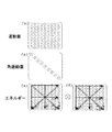
- the basis functions when subgroups based on angular momentum can be defined when taking the extended spur of the energy matrix shown in the table or the extended spur of the energy matrix of the back. That is, the first is a method in which the angular momentum quantum numbers are arranged in ascending order. The second is a method in which the main quantum numbers are arranged in ascending order. Given these in turn, ⁇ i and a one-dimensional index, and creating a symmetric product and an anti-symmetric product ⁇ i ⁇ k ⁇ ⁇ k ⁇ i as a two-dimensional matrix product, the first and second terms I and k are exchanged across a diagonal component.
- i and k are expressed using two indexes of angular momentum quantum number and main quantum number, in the case of the first arrangement, the main quantum number is simply within the submatrix of the same combination of angular momentum quantum numbers.
- the second arrangement is adopted, the expression will be slightly different from this, so care must be taken.
- the first arrangement is better when creating the product of the ( ⁇ ) and ( ⁇ ) planes, and the second arrangement when creating the product of the ( ⁇ ) and ( ⁇ ) planes. Turned out to be excellent. This is based on the premise that the first arrangement can be treated as an independent system between different angular momentum quantum numbers, and that it is satisfied by the expansion of the basis function of the completely orthogonal system in the same plane. means. On the other hand, the second way of arrangement shows that even if it is between different angular momentum quantum numbers, it is possible to describe how the basis functions between the adjacent main quantum numbers are more closely related. This is probably because the HVC surface does not describe a completely independent system.
- a specific example of a submatrix sum for actually dividing an energy matrix into submatrices of angular momentum to form an extended spur will be shown.
- the following is expressed in the form of a composite system of two basis functions forming a submatrix, and the sum of the submatrix and submatrix is also shown.
- the symbol e is used when the angular momentum coordinate axis is in the standard state
- the symbol i is used when the angular momentum coordinate axis is inverted.
- the standard state and the inverted state will be described simultaneously using ⁇ symbols. Since the axis inversion operation of the angular momentum for describing the back view is performed only on one basis function constituting the matrix, only the odd function on one color plane side is inverted. Components that disappear through these operations are not described.
- the energy matrix is displayed as a partial matrix in the unit of angular momentum as described above, and the submatrix of the eigenstate with the same angular momentum quantum number is different in the diagonal position. If the submatrix of the mixed state (hybridization term) with the angular motion quantum number appears in the off-diagonal position, the results consistent with the physical meaning can be obtained. In other words, when comparing the image alignment for energy elements made from diagonal submatrices and the image alignment for energy elements made from off-diagonal submatrices, clouds emerge from the mountains in the mixed state of off-diagonal components. It was found that it has the ability to capture very dynamic pictures such as scenes.
- ⁇ Higher-order invariants of texture> Expand the texture distribution function into a spherical Bessel.
- the spherical Bessel function is extended to the negative region and expanded to a double series of roots and orders that form a complete system. Since the spherical Bessel function represents a radial wave function, the expansion relating to the root corresponds to the principal quantum number n, and the expansion relating to the order corresponds to the orientation quantum number (orbital angular momentum quantum number) l.
- These orbits form the periodic table of elements
- the d orbital corresponds to the transition metal
- the f orbit corresponds to the description of the electron system of the lanthanoid and actinoid elements.
- the variable x takes the values of ⁇ H, ⁇ V, and ⁇ C.
- ( ⁇ ) is used to represent the difference in color plane, but ⁇ ln in the spherical Bessel function is used to represent the root position.
- Smirnov's "Higher Mathematics Curriculum” contains an approximate expression for the zero point of the Bessel function. Then, by deducting it into an approximate expression to represent the zero of the spherical Bessel function, and introducing a correction factor of 1/2 with respect to the second term without changing the first term, an error within 3% at all zeros Since it was found that the expansion coefficient can be approximated by the following equation, the following equation is used to calculate the expansion coefficient over the p orbit.
- angular momentum, and energy which are mechanical invariants, from the distribution function, derive as much as possible components that can be evaluated independently to describe the shape of the distribution function. That is, as in the case of color, in constructing energy and angular momentum, f ( ⁇ x) obtained by axially inverting the distribution function f (x) is also added to the consideration.
- the physical meaning of axis inversion corresponds to edge code inversion.
- the axis inversion operation corresponds to an operation to invert the parity of angular momentum.
- the angular momentum quantum numbers are classified into subgroups based on the difference between the properties of the even function and the odd function, and an orientation quantum number is assigned to each subgroup.
- the wave function of the s and d orbits has an even parity
- the wave function of the p and f orbits has an odd parity.
- a basis function group represented by a spherical Bessel function has a parity represented by ( ⁇ 1) ⁇ l using an angular momentum quantum number l with respect to inversion of coordinate axes.
- the momentum element p n the angular momentum element M n , and the energy element E n when the axis of the angular momentum describing the system is not reversed are first constructed.
- each of them is led to an element of about twice the axis of angular momentum inverted.
- the number N of expansion coefficients is set to 100.
- Angular momentum element M n examples include the following.
- (In case of expansion by s, p, d, f orbit) 1 (c 11 ( ⁇ ) + c 12 ( ⁇ ) + ... + c 1N ( ⁇ ) ) +2 (c 21 ( ⁇ ) + c 22 ( ⁇ ) + ...
- the linear sum of the expansion coefficient of the odd function gives a macroscopic index for evaluating how far the asymmetry of the distribution function extends to show its properties
- the expansion coefficient of the even function gives a macroscopic index for evaluating the extent to which the distribution function spreads in a tail-extracting manner, and preserves the overall spread property as angular momentum It can be a macroscopic physical quantity.
- the first bundling method represents the intrinsic state of angular momentum.
- the second to fourth bundling methods represent a mixed state of angular momentum.
- the mixed state is a state in which the angular momentum has a hybrid orbit, for example, a subgroup called sd hybridization is created between sd.
- 17A to 17D are matrix diagrams showing how the following four expanded spurs are configured. These are defined to include the case of only s, p orbitals.
- the spin angular momentum S defined by the color of the higher-order system the energy element E n by the inner product of the orbital angular momentum L defined order based texture.
- the symbol S is used for the higher-order color subsystem and L is used for the higher-order texture subsystem.
- Rotational energy of low-order color system The low-order system has already been introduced as a product of ⁇ and ⁇ , which is the quadratic form of the fluctuation term of the model Hamiltonian. 3) Rotational energy of higher order system of texture In the same way as the above-mentioned spin-spin interaction, rotational energy by the orbital angular momentum of the coordinate system can be defined.
- an angular momentum L ′ vector independent of the coordinate axis inversion is defined.
- the case where both angular momentums are reversed is an independent energy element. Therefore, the number of energy elements is three times six.
- the intensity Qi of the sensibility impression regarding a certain adjective i is represented by a linear sum of individual energy elements emitted by each image.
- the size and sign of the energy element that is regarded as important for each adjective is different, and it appears in the form of a linear coupling coefficient as a property that characterizes the adjective.
- mechanical invariants which are image features, are physical quantities converted from purely microscopic image information to macroscopic image information, and what needs to be modeled is aggregated in the linear combination coefficient.
- the prior learning of the model for determining the linear combination coefficient is also based on the statistical average of the statistical group of the image group, following the basic concept of statistical physics.
- each subsystem is described with additive features, so the number of combined features when integrating subsystems such as inter-spindle synthesis is the most reduced. It is expressed by a simple simple sum. The number is on the order of 10,000, which is about the same as the total number of sensitivity adjectives.
- the linear coupling coefficient also plays a role in matching energy and physical dimensions. Therefore, when all the mechanical invariants are used, after determining the factor structure of the linear coupling coefficient in energy unit, momentum unit, and angular momentum unit during model learning, the coupling coefficient for scaling the whole between the three It is necessary to decide again. In addition to matching the dimensions, this also determines which invariants play an important role among the three. In general, the role of momentum and angular momentum decreases when statistical averaging is performed on many model images.
- ⁇ State density and adjective model> If macroscopic energy is derived from image information and has a value at a certain energy level, the energy at that energy level is emitted by that amount, and a state exists at that energy level. Means. If the value of an energy element at an energy level is zero, the image does not emit that energy element at all, and no state exists at that level. The energy value may take a negative value.
- ⁇ > in the denominator represents a statistical average of images that are models of general images
- ⁇ > i represents a statistical average of all adjectives prepared by the image search system.
- the adjective impression of how strong an image is with respect to the average image It is possible to quantify whether or not it is emitting on an absolute basis. Therefore, an absolute impression that includes not only a relative impression evaluation within a single image or only within one adjective but also an evaluation criterion for the mutual magnitude relationship between adjectives from an absolute image criterion. It becomes possible to evaluate the sensitivity. Therefore, the standardization of Qi is only standardized so that it falls within the [-1,1] interval in the average range, and sometimes it may exceed that range.
- the deviation value itself is directly Represents the importance of the energy element for that adjective.
- the average value of the distribution of the general image is set to zero and the deviation value represented by the interval of [-1,1] at both ends is used, it can be directly used as a linear combination coefficient.
- This deviation value is assumed to be a normal distribution whose width is given by the standard deviation value of the general image distribution, and is given in the form of an integral value of the distribution function of the interval from the average value of the general distribution to the average value of the model image .
- the error of the deviation value can be calculated by giving the average value and the standard deviation value of the general image distribution and the model image distribution, respectively.
- the distribution of energy values in the adjective model image means that the energy values fluctuate. Therefore, it can be said that the sensitivity description method that determines the sensitivity using a large number of images has a correspondence with the Gibbs distribution (canonical distribution) of statistical physics that describes the macroscopic physical quantity of the fluctuation distribution of energy values ( Reference E4).
- the model adjective image is reduced to the limit of only one image, the macroscopic energy of the system without the fluctuation of the energy value is fixed in the general image distribution.
- a single similar image search corresponds to a macroscopic physical quantity energy value of the image, and a description of the microcanonical distribution of statistical physics in which each of momentum and angular momentum is described by a delta function.
- the method of dynamically describing sensibility has the capability of seamlessly describing a sensibility image search composed of a plurality of images from a single similar image search. The method only changes the number of model images for determining the linear combination coefficient to the number of target image groups.
- FIG. 19 is an imaginary diagram of a hierarchical structure of pyramids. The energy factor of the additional factor plays a role in separating states by solving the conventional energy level degeneracy.
- the adjective energy Pi, j of the subsystem defined as the inner product of the state density function ⁇ (E n ) and the linear coupling coefficient ⁇ (E n ) (here, a symbol to distinguish from the adjective energy Qi of the entire system is introduced)
- the linear combination coefficient k can be determined through exactly the same process that has been performed for each energy element in the subsystem until now. In other words, regarding the energy index obtained by partial summation of the linear combination, it is examined how the image group of the general image model is distributed, and the deviation value indicates where the image group of the adjective model is distributed. Is used to determine the linear combination coefficient k.
- the linear combination coefficient k obtained in this way elucidates the effect ratio of the subsystem, which subsystem element of color, texture, and composition actually determines the impression of the adjective by acting strongly on the adjective. Will lead to.
- a value in the range of [-1,1] can be taken for the linear combination coefficient k of the subsystem, but when an experiment is actually performed, a result that takes only a positive value is given. This is in accord with the mystery of the role inherent in the subsystem that only changes the rate of action of the factor structure.
- FIG. 20 is an energy band diagram for color and texture. If the state density function is illustrated in the order of energy levels, a scalar invariant of a lower order system becomes a discrete energy level, and a vector invariant of a higher order system becomes a continuous energy level. This is an aggregate of atoms that has an Avogadro number, for example, a metallic material, the inner electron orbit is in a discrete energy level close to the atomic orbit, and the outer electron orbit is the electron orbit of an adjacent atom.
- a state density diagram similar to a system with an energy band structure in a conduction band consisting of dense energy levels with the overlapping of layers is completed.
- the energy band diagram describing the sensitivity of one image looks different. That is, a state taking a positive energy value (state density diagram on the right side of FIG. 21) and a state taking a negative energy value (state density diagram on the left side of FIG. 21) go right or left at an arbitrary level.
- the state density is allowed to be arbitrarily packed. This can be interpreted as describing the nature of the Bose particle in a sense. Therefore, condensation in which the state concentrates at a certain energy level may occur as a state system of the image.
- the Chebyshev function chosen to be optimal for describing higher-order invariants of color is actually a special function that can only describe the state of angular momentum 1 systems. It matches exactly what is there.
- the photon forming the image is a system having a spin angular momentum of 1 in terms of quantum mechanics. From the state of the energy band diagram, it can be seen that the color spin system describes a very detailed factor structure.
- the texture system described using a spherical Bessel function suitable for describing a radial wave function on one side can be seen to describe a very rough energy structure. This is because when considering the energy level of a material atom, the radial wave function determines the large energy level, and then the wave function in the direction of the zenith angle and azimuthal angle has the next fine energy level. This is very similar to the relationship in which the spin system determines a finer energy level. However, when it comes to the electronic structure of a substance such as a solid, the spin system begins to play a major role in ferromagnets, for example, so the magnitude relationship of the degree of separation of the energy levels is agglomeration of atoms. The system cannot be described in general.
- ⁇ Image temperature> In an image system, the temperature of the system including both steady state and unsteady state is defined. Temperature is positioned as the sum of the number of energy states. Therefore, the quantum state E n of the energy, the temperature norm of a vector when the vector representation for state n. This corresponds to the denominator normalization factor when the energy density of states is defined. The number of energy states that each image can take is different, and the temperature is also different for each image. Therefore, the concept of image temperature can be defined. It is necessary to first define the temperature of the image in the subsystem unit that shares the accounting method of the number of states. Also, the image temperature has the same dimension as energy.
- the vector norm takes a value greater than or equal to zero, which satisfies the condition that the temperature satisfies. Also, when there is no energy state number, the image system is at absolute zero. However, since a conjugate space in which the uncertainty principle works is described as the projection plane of the subsystem at the same time, it is difficult to create an image that has absolute zero.
- the entropy of the entire system can be defined. If a represents a subsystem,
- Entropy is a dimensionless quantity.
- the entropy of subsystem a is calculated by the following formula. Integration is performed only in the interval where the value of the distribution function is finite. The interval with zero value shall be skipped. However, the number of states of the distribution function is assumed to be standardized. Therefore, it always takes a value greater than or equal to zero to satisfy the entropy requirement.
- thermodynamic invariant of heat quantity Q TS
- the low temperature system is close to a monochrome image and cool
- the image of the impression is colorful in the high temperature system, and the image of the hot impression including the red system and the highland scenery in midsummer is divided.
- images with tightly packed uniform texture are low-temperature systems, and summary images with proper composition and main subjects are displayed. It is characterized by gathering in high temperature systems.
- the low-order invariant subsystems of the texture are divided into a low-temperature system with a quiet and quiet impression, and a high-temperature system that has a lot of objects and people gathered together and is full of emotion and emotion.
- the high-order invariant subsystem of color is divided into a low-temperature system with a vivid impression often found in Japanese structures and sunny clothes, and a high-temperature system with a deep, dark hue.
- TS invariants play an important role in determining the properties of subsystems and verifying whether they are dealing with independent subsystems.
- the value of the energy E n is expressed as an n-dimensional vector for the energy level n, and a scalar invariant TS is further added to define the free energy F.
- thermodynamic physical quantity that represents the macroscopic properties of the image system itself. From the macroscopic nature of this image, it is possible to measure how much the nature of a certain adjective is emitted by taking the inner product with the linear combination coefficient ⁇ vector that is a model of the adjective.
- 1 / ⁇ S> represents the Boltzmann constant k defined in the subsystem unit. This is because the Planck's constant h for measuring the number of states in each subsystem is different, so that it plays an important role in matching both scales when integrating subsystems.
- the denominator standardization method plays a very important role. The basic idea is that it should be brought to the denominator with the statistical average as much as possible. If the purpose is to fit the inner product to the interval [-1,1], it may be possible to bring the absolute value of the numerator to the denominator. The energy measurement as the whole system will fail.
- E-TS means the thermodynamic work done through them (see reference E6).
- the microscopic state of the image system pixel value distribution
- E and heat quantity TS energy E and heat quantity TS
- thermodynamic work F is performed on the human brain. Induces sensitivity. Therefore, the energy band diagram calculated from only the signal value distribution of the image system represents the macroscopic nature of the image itself, whereas the state distribution diagram obtained by multiplying them by the linear combination coefficient ⁇ vector It is considered that the distribution map of sensibility in the brain is visually quantified.
- ⁇ Correlation matrix of adjectives> An example of an adjective correlation matrix w ij clarified in the fifth embodiment for clarifying a correlation between adjectives based on a certain person will be shown. It is a value in the range that handles the subsystems up to color and texture. i and j are assigned adjective numbers in the order of “fresh”, “lively”, “rough”, “moist”.
- the average is calculated with an equal weight for the model image.
- the weight of 0.2 sheets applies to the psychological degree 1
- the weight of 0.4 sheets corresponds to the psychological degree 2
- the calculation is performed so that the one with a psychological degree of 5 receives the weight evaluation for one sheet.
- the error of the average value can be evaluated by evaluating the average value of the model image and the spread width of the distribution with the standard deviation. That is, in the process of calculating the deviation value indicating the position of the average value of the model image with respect to the distribution of the general image, by combining these values, the average value of the general image, and the standard deviation thereof, an error of the deviation value based on the definition is calculated. If it is also evaluated, it is possible to obtain data that combines the evaluation reliability of the deviation value.
- a stable sensibility retrieval system when there are a large number of adjective model images will be described.
- a sensitivity search system capable of dealing with a small number of adjective model images will be described.
- a similar image search system for a single image will be described.
- f (H) the probability density of the neutral hue is described in one bin called f (N).
- the entropy S is calculated from the distribution function f (x). When the value of the distribution function is 0, it is excluded from the integration interval in the sense that the state is not taken. When the color surface of the distribution function is distinguished by ( ⁇ ), entropy is calculated from the distribution functions of the H, V, and C surfaces, and the sum of those is projected to the lower-order system of the color. To express. This value is S Fo .
- the average value and the deviation value are calculated on the axis in which the hue circle is made one-dimensional using the distribution function excluding the neutral component.
- the calculated energy elements E n of the energy elements E n of is defined as follows. The values of energy elements are all described in the range [-1,1].
- Subsystem temperature calculation When the energy element values are collectively expressed as a vector, the energy vector of the subsystem can be defined. By calculating the norm of the energy vector of the subsystem, the image temperature T for the subsystem can be defined.
- ⁇ > represents a statistical average regarding an arbitrary general image. Therefore, for ⁇ S>, it is necessary to calculate the entropy of an image for a large number of arbitrary general images prepared in advance and to calculate the average value thereof in advance.
- 1 / ⁇ S> serves as a Boltzmann constant k for linking the number of microscopic states in the phase space to a macroscopic physical quantity called entropy based on the Planck constant h defined in this subsystem. That is, the number of states in the phase space
- the temperature is measured by kT via the Boltzmann constant k to connect the temperature with the energy amount.
- the definition of the Planck constant varies depending on the subsystem, such an absolutely invariant physical constant cannot be defined.
- the entropy S is calculated from the distribution function f (k). When the value of the distribution function is 0, it is excluded from the integration interval in the sense that the state is not taken. When the color surface of the distribution function is distinguished by ( ⁇ ), the entropy is calculated from the distribution functions of the H, V, and C surfaces, and the sum of these is projected into the higher-order system of the color. To express. This value to S F.
- a pure spur of the energy matrix i.e. the sum of the diagonal elements, using a relationship guaranteed by the Schwarz inequality so that each of them falls within the range [-1,1]. Standardize with. Therefore, the normalization operation cannot be performed only in the steady state constructed only by pure spurs. Standardize all other energy elements and define an extended spur. Since the value of the pure diagonal sum is defined in the range of [-1,1] for each expansion coefficient of the distribution function, the value in the range of [0,1] may be slightly extended. I want.
- the energy eigenvalue represents the absolute amount of energy
- the energy eigenvalue must have a finite value and the linear combination coefficient must have a non-zero value when finally taking these linear combinations. So it makes a different meaning.
- the energy eigenvalue indicates the presence or absence of an energy element emitted from the image itself, and the linear combination coefficient merely indicates whether or not it is an important element for a certain adjective.
- the energy eigenvalue must therefore be measured on an absolute basis.
- the zero-point energy ⁇ 0 is added to the diagonal-sum energy from the beginning, and it corresponds to the zero-point energy. You may make it define by subtracting a minute.
- the number of elements of the expansion coefficient is divided into N half.
- Subsystem temperature calculation In the same way as described above, the energy vector of the subsystem and the temperature T of the subsystem can be defined.
- the number of bins in the histogram is 200.
- the distribution function is quantized in bin units and cannot be described with higher accuracy.
- the distribution function is also expressed as follows. f ( ⁇ H), f ( ⁇ V), f ( ⁇ C)
- the entropy S is calculated from the distribution function f (x). When the value of the distribution function is 0, it is excluded from the integration interval in the sense that the state is not taken. When the color surface of the distribution function is distinguished by ( ⁇ ), entropy is calculated from the distribution functions of the edge images on the H, V, and C planes, and the sum of these is projected onto the lower order system of the texture. Represents the entropy of. This value is S Go .
- the calculated energy elements E n of the energy elements E n of is defined as follows. These values are all defined by real numbers.
- the Boltzmann constant of this subsystem is measured by the reciprocal of the statistical average of any image of the entropy of this subsystem.
- the entropy S is calculated from the distribution function f (l, k). When the value of the distribution function is 0, it is excluded from the integration interval in the sense that the state is not taken. When the color plane of the distribution function is represented by ( ⁇ ), the entropy is calculated from the distribution functions of the edge images on the H, V, and C planes, and the sum of these is projected onto the higher order system of the texture. Represents the entropy of. This value is S G.
- the Boltzmann constant of this subsystem is measured by the reciprocal of the statistical average of any image of the entropy of this subsystem.
- Distribution function p (x) represents the image frequency of the general image can take in unit energy interval taken by the real-valued E n, by delimiting energy interval as the bottle, the frequency distribution function.
- Adjective Model Image For each of the prepared general image models, psychological impression evaluation is performed as to whether or not it corresponds to the i th adjective, and distribution data of the adjective model image is created. There are two ways to create this, and either one can be used. That is, in the case of simply corresponding or not applicable, an integer of 1 or 0 is assigned, and an image assigned 1 is used as an image having the same weight. Then, the distribution function q (x) of the adjective model image group is constructed using the corresponding image group. The other is a method in which a non-applicable case is set to 0, and a psychological absolute impression degree in the applicable case is evaluated on a 5-level scale of 1-5.
- a weight of 1.0 is assigned to an image of 5 evaluations
- a weight of 0.8 is applied to an image of 4 evaluations
- a weight of 0.6 is applied to an image of 3 evaluations.
- a frequency distribution q (x) described below is constructed by assigning a weight of 0.4 to an image of 2 evaluations and a weight of 0.2 to an image of 1 evaluation.
- the linear combination coefficients for the energy elements E n corresponding to the i-th adjective alpha i (E n) can be expressed as follows using the error function erf (x).
- the linear combination coefficient is defined to be 0 when positioned at the same position as the average value of the general model image, and ⁇ 1 when positioned at both ends. Further, the fluctuation of the deviation value of the adjective model image group, that is, the error ⁇ i (E n ) of the linear combination coefficient can be evaluated.
- a1 corresponds to a low-order system of color
- a2 corresponds to a high-order system of color
- a3 corresponds to a low-order system of texture
- a4 corresponds to a high-order system of texture, and the like.
- ⁇ > a represents the statistical average between all subsystems. That is, if the number of subsystems considered is n a
- the standardization of the denominator follows the idea that statistical averaging should be performed as much as possible.
- the difference in the number of states that is, the difference in entropy due to the difference in the number of bins of the distribution function that is defined differently depending on the subsystem is absorbed, and different subsystems can be put on the common earth. That is, the definition of the Planck constant and the Boltzmann constant that differ depending on the subsystem is absorbed here, and the energy physical quantity Pi on a scale that can be handled in the same way is calculated.
- the term of the square root of the denominator can be interpreted as a correction term that is required when the physical constant varies depending on the subsystem.
- the norm average of the average temperature and adjective vector is a standardization to absorb the difference in the number of energy elements that can be defined by the subsystem.
- the normalization by the norm statistical average for placing the subsystems on the common earth plays an extremely important role in defining the absolute physical quantity.
- a large amount of arbitrary general images are prepared, and the entropy value and temperature value are experimentally examined for each subsystem. These numbers show how important the standardization procedure is to integrate subsystems.
- Steps for determining the linear combination coefficient is performed by the same procedure as conducted in order to determine one single ⁇ i relative energy elements E n described above. That is, with the partial sum Pi, j as a variable x, the average value for the distribution of the general model image is m p , its standard deviation ⁇ p , the average value for the adjective model image distribution is m q , and its standard deviation ⁇ q is determined and the linear combination coefficient is determined in the same manner.
- ⁇ > represents an average for a general model image
- ⁇ > i represents an average for an adjective.
- the energy band diagrams shown so far are drawn using ⁇ (E n ) in a form including the weighting coefficient k of this subsystem.
- the density of states is considered as ⁇ (E n ) ⁇ max (E n ) as the maximum for the gamut region ⁇ max (E n ) that swings to the maximum in the energy elements used in the general model image.
- the range is painted as an energy band model.
- Adjective search processing when an energy band model is constructed by combining a general model and an adjective model for learning, an image with an impression similar to that of the i-th adjective is used as an adjective energy for another database image.
- images are arranged in the order of Qi, it becomes a shape close to a normal distribution, and a region having a high deviation value of the upper group can be presented as a target image.
- energy band model an average model common to all people can be taken, and models specific to those cultural spheres can be constructed according to differences in countries, cultures, and languages. Alternatively, an individual energy band model that reflects differences in personal-level preferences can be constructed. Therefore, the energy band structure model adopted by this image retrieval system can be used as a tool for quantitatively elucidating the structure of human sensitivity.
- the idea of obtaining the linear combination coefficient by the deviation value is extended, and the final obtained Qi value is a model once more whether or not the adjective model image is gathered in the upper group compared to the general model image. This can be confirmed by obtaining the deviation value of the image group from the general model of Qi. As a result, the validity of the theoretical model and the sufficiency of the feature amount to be handled can be verified.
- the correlation matrix of the adjective shows a value close to a symmetric matrix is to verify the validity of whether or not the image group selected in the model construction process selects a general random image.
- it is desirable that all diagonal components are 1 as described above. If the diagonal component has not been reached, the feature amount for capturing the adjective is insufficient, or the portion where the theoretical model hypothesis does not hold. Since it means that it exists, it gives a good evaluation index for building a search system.
- the image temperatures T E , T p , T M related to the subsystem can be defined in units of mechanical invariants.
- model adjective vectors are determined for each of the free energy vector, free momentum vector, and free angular momentum vector. It is assumed that the deviation value is determined through the same process for the TS invariant. That is,
- the adjective energy P i of the subsystem is expressed by taking these inner products.
- Adjective retrieval processing (seventh embodiment] (Similar image search of single image: 3 steps integration of “energy + momentum + angular momentum”)
- Similar image search of single image 3 steps integration of “energy + momentum + angular momentum”
- an example of constructing an adjective model using a minority model has been described. If you take this to the limit, you can use it to search for a single similar image. That is, it is possible to extract an image having a similar overall impression of one illustrated image through description of energy, momentum, and angular momentum, which are macroscopic physical quantities.
- the method of the sixth embodiment includes the method of the fifth embodiment. This is because as the number of model images increases, the role of momentum and angular momentum decreases, and their linear combination coefficients converge to a value close to zero automatically by statistical averaging. Therefore, the method of the sixth embodiment can be seamlessly realized from single image search to small-model sensitivity search, and further to multiple-model sensitivity search.
- the Munsell color space is a uniform color space that guarantees perceptual equality. Therefore, the Munsell value itself in the real space description provides a color space in which the uniformity of the space is guaranteed.
- a shape such as a one-dimensional histogram
- there is a constraint condition that the distribution function of the histogram must satisfy and humans recognize the difference in the shape of the part where the degree of freedom exists, taking the constraint condition into consideration.
- the frequency expansion is performed using a basis function having the same property as the constraint condition, the expansion coefficient can be regarded as being converted into a space that recognizes the difference in the shape of the portion where the degree of freedom exists. That is, the basis function space in the frequency space description provides a recognition space in which the uniformity of the space is guaranteed.
- the expansion coefficient defines the momentum.
- the mass is assumed to be a constant of 1, it can be understood that the momentum represents velocity. Therefore, in image recognition, the Munsell value and frequency expansion coefficient taken by each image can be regarded as momentum, and can be a feature quantity that satisfies the conservation of momentum between images.
- the Munsell value taken by each image or the angular momentum derived from the frequency expansion coefficient can be a feature quantity that can preserve the angular momentum between the images.
- the uniformity of time in the image system is positioned as any scene can be generated with equal probability as an image capturing an arbitrary scene. Therefore, if the physical quantity of energy expressed in the quadratic form of momentum or velocity is defined, the energy conservation law is established, so that the feature quantity of the image is between images that cause the same image recognition and the same image sensitivity. This means that it can be an effective feature amount having a common value.
- the quantity can be a physical quantity that is effectively stored between images.
- These are all additive physical quantities, and it can be assumed that the final image recognition strength and impression impression are expressed by a linear combination of these physical quantities. This is the “linear model of sensitivity” hypothesis.
- a distribution function representing an independent subsystem such as color and edge is derived from an image, and the distribution function is projected onto a real space or a frequency space equal recognition space, and further projected onto a feature quantity consisting of energy, momentum, and angular momentum.
- the operation is performed on each of a specific image group causing a certain common sensibility and a certain common object recognition at the same time as a general image group of a general large amount of images.
- projective expression is expressed in a perceptual space and linear space for image recognition, and it is investigated how the specific image group is distributed in the general image group on the projection plane, and the specificity is determined by the degree of the bias.
- the final impression level of the individual image can be converted into an absolute value.
- the one-dimensional distribution of gradations has two main axes, the one-dimensional distribution function of the color already handled and the one-dimensional distribution function of the edge.
- the two-dimensional distribution of the composition has been treated as one principal axis in the description up to the sixth embodiment, but actually two two-dimensional distribution functions of color and edge exist as principal axes. Accordingly, the four principal axis systems are basically composed of the one-dimensional distribution of gradation and the two-dimensional distribution of composition.
- the sub-system that has been called texture until now will be called edge again.
- both one-dimensional color histograms and edge histograms represent frequency distributions, they are all defined as positive values. If normalized by the sum of the frequencies, they are expressed by probability density and can be called distribution functions. Since all pixel values of the two-dimensional color plane are defined as positive values, a distribution function can be obtained by normalizing the sum of pixel values. However, since the value of the edge surface of the two-dimensional system has both positive and negative values, it is not simply a distribution function. Therefore, the distribution function of the edge surface of the two-dimensional system is defined by squaring the value of the edge surface integrated with multiple resolutions so that all are defined as zero or more values, and the probability density of the edge surface distribution function is defined as The distribution function.
- the frequency space description of one-dimensional distribution function first, only the range where the distribution function is actually distributed as values is taken out, the coordinates of the start point and end point are defined in that section, and the contrast is maximized. To evaluate the distribution shape. Therefore, the frequency description plays a role of evaluating the shape of the distribution function on a relative scale.
- the absolute signal value of the gradation value is used as it is, as in the case of the one-dimensional distribution function, for the coordinate setting relating to the signal intensity of the brightness level.
- the absolute length is defined as it is. That is, the information regarding the difference in aspect ratio is defined in the real space, and the position can be identified.
- the distance is relativized in the vertical and horizontal directions, and the contrast is also relativized in the distribution range of the gradation, and plays the role of evaluating the shape of the distribution function.
- the real space representation it plays the role of defining the absolute position in the vertical and horizontal directions and the strength of the absolute signal within the gradation range.
- the value of the expansion coefficient that is frequency-expanded by the basis function after being relativized within the distribution range of the value of the distribution function in the frequency expression can always fall within the range of [-1,1]. If the expansion coefficient in the frequency space is positioned as speed, there is a limit point in the range that the speed can take, and this can be considered in correspondence with the speed of light.
- H (x, y), V (x, y), and C (x, y) representing the two-dimensional Munsell value distribution represent the momentum value distribution.
- symbol of momentum schematically Is used to represent a physical quantity having a dimension of (brightness intensity) ⁇ (space position vector).
- the average term and the fluctuation term are described by the product of the brightness direction and the spatial direction, respectively, the average term is actually described by a vector and the fluctuation term is described by a tensor. Details are defined in the embodiment.
- the motion described by this model Hamiltonian is captured in association with the motion of a rigid body on a two-dimensional plane.
- the distribution of intensity values in the brightness direction is positioned as having a dimension relating to the motion of the rigid body, that is, a dimension of the rate of change per unit time.
- the distribution in the spatial direction describes the form factor in a stationary state of the rigid body, and is positioned as having a dimension related to distance.
- the average term is a description about the translational motion of the rigid body
- the fluctuation term is a description about the rotational motion of the rigid body.
- the momentum, angular momentum, and energy related to the motion of the rigid body are defined in the following forms. That is, the momentum and the angular momentum are in the primary form of intensity in the brightness direction, and the energy is in the secondary form of intensity in the brightness direction.
- FIG. 25 is a diagram showing the relationship of elements related to the construction of a low-order invariant of composition.
- the momentum corresponds to an average term
- the angular momentum corresponds to a spread term or a fluctuation term.
- the relationship between the feature amount derived from the one-dimensional distribution function of the gradation and the feature amount derived from the two-dimensional distribution function of the composition will be described.
- the subsystem defined by the one-dimensional distribution function is described with a correlation through the brightness factor portion.
- the one-dimensional color distribution system and the two-dimensional color distribution system derive a feature amount that overlaps the brightness factor.
- a feature amount having an overlap in the brightness factor portion is also derived for the one-dimensional distribution subsystem of the edge and the two-dimensional distribution of the edge.
- information about spatial factors is newly added to the feature quantity derived from the two-dimensional distribution, and elements that are independent of the feature quantity derived from the one-dimensional distribution are described.
- the Chebyshev function is used to describe the frequency by projecting the one-dimensional color distribution function to the Hilbert space
- the spherical vessel is used to describe the frequency by projecting the one-dimensional distribution function of the edge to the Hilbert space.
- Functions have been used. This is because a basis function that equalizes shape recognition suitable for the constraint conditions that the shape of the distribution function can take is selected.
- the shape of the distribution function with an expansion coefficient representing the frequency distribution of the basis function, the shape is mapped to the uniform recognition space.
- the color side should be described by a special function belonging to the hypergeometric function
- the edge side should be described by a special function belonging to the confluent hypergeometric function.
- This principle is applied to the selection of basis functions when expressing the remaining two principal axes, the two-dimensional color distribution function and the two-dimensional edge distribution function, in the Hilbert space.
- the Legendre function is selected as a basis function suitable for expressing the frequency of the two-dimensional color distribution function.
- a Fourier function is selected as a basis function suitable for expressing the frequency of the two-dimensional distribution function of the edge. The reason for selection is described below.
- the Legendre ⁇ function is a kind of hypergeometric function and is suitable for describing color distribution.
- the Legendre function P m l (x) is defined by two indices, the magnetic quantum number m and the orientation quantum number l. Between basis functions with different orientation quantum numbers l, the orthogonality of the basis functions has a uniform spatial weight. Have orthogonality.
- the relational expression of the orthogonality of the Legendre function and the specific expression on the low frequency side of the basis function of the Legendre function are given.
- FIG. 26 is a graph of P 2 (x), P 3 (x,) P 4 (x), P 5 (x) in the Legendre polynomial.
- the Legendre function is a function suitable for describing the properties of the electric multipole distribution when a charge is placed at the position of this singular point.
- a notch of framing the composition is added to a uniformly distributed subject image.
- This cut point becomes a singular point as an image, and acts as a framing effect when the shape is recognized from the compositional side of the image.
- the shape distribution seen from the singular point enables high-dimensional moment analysis in the frequency space of the spatial distribution using the Legendre power function including the concept of multipole.
- the image has singular points that correspond to the north and south poles on the earth on the right and left ends, or the upper and lower ends, but the space between them is nevertheless treated uniformly. This matches the property of framing the space and cutting out the composition.
- the color distribution has the property that gradation appears like a blue sky.
- the Legendre function is a function suitable for expressing the two-dimensional color distribution function in a very compact frequency because the first wave has the basis function. Refer to Document B3 for a detailed explanation of the Legendre function.
- the Fourier function is a differential equation without singularities. It corresponds to the function of classification.
- the two-dimensional distribution function of the edge is not described as an edge surface having positive and negative values, but is described by a distribution of values obtained by squaring them.
- the edge surface is detected from the color surface, the image has a value close to zero at most. Since it is squared on it, the distribution of values has the property of a very smooth waveform.
- the image obtained in this way is mostly black except for the high-contrast edge. If the right and left edges are connected to form a cylinder, or the top and bottom images are connected to form a cylinder. Even if it is shaped, it is an image having the property of connecting smoothly without recognizing an abnormal cut due to a difference in distribution. This means that it is suitable to describe an infinitely wide waveform having no singular points at both ends of the image.
- a Fourier function that has no singularity and has a property that the boundary condition at both ends has a value of zero or a derivative is zero matches the characteristics of the waveform distribution of this image. Furthermore, the Fourier function also has the property of uniformly handling the space, which is an important property when dealing with composition. The relational expression of the orthogonality of the Fourier function by a uniform weight function is described.
- the variables of the image are separated, the one-dimensional distribution function of the color is the property related to one independent variable of the spin system, the one-dimensional distribution function of the edge is one of the radial direction Position the properties related to the independent variables as the two-dimensional distribution function of the color describes the properties of the two independent variables in the zenith angle direction, and the two-dimensional distribution function of the edge describes the properties of the two independent variables in the azimuth direction. .
- the two-dimensional distribution function of the edge describes the properties of the two independent variables in the azimuth direction.
- the spherical Bessel expansion coefficient is determined so as to satisfy only the orthogonality related to the root of the quantum number n independently in a closed state in this subsystem.
- the orthogonality with respect to the order m bears the orthogonality of the basis function with respect to the quantum number m of the Fourier function that expands the two-dimensional distribution of edges. Therefore, the expansion coefficient of the Legendre power function is determined so as to satisfy only the orthogonality with respect to the quantum number l alone in a closed state in this subsystem.
- the edge one-dimensional distribution function subsystem and the color two-dimensional distribution function subsystem and further, the color two-dimensional distribution function subsystem and the edge two-dimensional distribution function.
- the edge two-dimensional distribution function subsystem and the edge two-dimensional distribution function There is a correlation between the subsystems in which the orthogonality of the basis function is reflected on one side by simultaneously describing the distribution function between the subsystems.
- the distribution function of the entire image is represented by the product of the distribution functions of the subsystems, so that each subsystem maintains statistical independence.
- the energy eigenvalue E n is derived.
- the eigenvalues of energy are derived from the differential equations that each subsystem satisfies.
- the energy eigenvalues of the entire system are represented by the sum of the energy eigenvalues derived in the respective subsystems. Therefore, the energy level which has been degenerated in a certain subsystem is solved by the action of other subsystems, and split energy levels are given.
- an image feature is described using only energy elements related to colors and edges in a one-dimensional system, it does not have the ability to distinguish the distribution of the two-dimensional composition, but the energy elements related to the composition are two-dimensional.
- the energy element can split and distinguish the energy levels of the previous one-dimensional system.
- the energy eigenvalues When deriving the energy eigenvalues when the axis is inverted, the energy eigenvalues are determined independently for each sub-system due to the statistical independence of the sub-systems. Therefore, as for the property of axis reversal, the energy element may be obtained by examining the property when the axis is reversed independently for each subsystem.
- the examination of the property of axis reversal is a unique matter only for the subsystem that describes the frequency space using a basis function consisting of an even function and an odd function. There is no such operation in the real space description.
- the energy element En is defined from the viewpoint of the energy dispersion relation in the frequency space (k space) and the irreducible expression.
- the two-dimensional expansion coefficient c ij projected onto the frequency space is converted into a one-dimensional array c i by some method, and a quadratic form of a symmetric product and an antisymmetric product is obtained from the product of the expansion coefficient of the ⁇ plane and the expansion coefficient of the ⁇ plane.
- energy is defined for the sake of clarity.
- the quadratic form sum is the sum of the products of all the elements of the two-dimensional plane of the ⁇ plane and the ⁇ plane.
- the problem of which point on the two-dimensional coefficient surface is the starting point and the direction of one ⁇ plane is selected in which direction, and how the other ⁇ surface is aligned with what is aligned in which direction is the starting point. is there.
- the question is whether there is an irreducible expression that most efficiently and compactly expresses the property of the coefficient distribution of the two-dimensional coefficient surface described by the product of the combination of the ⁇ and ⁇ surfaces. . This is constructed by comparing it with the method used to describe the nature of the energy band formed by the periodic crystal structure of solid state physics.
- the frequency-expanded two-dimensional expansion coefficient can be considered as extending a two-dimensional k-space represented by wave vectors kx and ky. It is defined that the highest frequency component in the x-axis direction is connected to the lowest frequency component in the x-axis direction. Similarly, in the y direction, it is defined that the highest frequency component in the y axis direction is connected to the lowest frequency component in the y axis direction. That is, the concept of super high frequency is that it recognizes as much as ultra low frequency as a whole because there are too many wave vibrations. This is a concept that is also introduced when energy elements are defined by extended spurs from the basis functions of the one-dimensional distribution function.
- n ⁇ 1 is c 00
- these two components can be considered as substantially equivalent points with a quantum number shifted by one.
- the connectivity-related properties of these expansion coefficients are the same as having a square Brillouin zone in k-space.
- cn -1, n-1 corresponds to (2 ⁇ / a, 2 ⁇ / a) in k-space To do.
- the definition of connecting the low frequency next to the highest frequency is equivalent to the property that the high frequency component is folded back as a low frequency component.
- n ⁇ n expansion coefficients have the same properties as the Brillouin zone of a square lattice in solid state physics.
- Is defined as a vector that defines the position and direction of the starting point of the rearrangement of the coefficients of the ⁇ plane.
- the energy dispersion relationship shifted by n pieces without shifting all n ⁇ n pieces is expressed as ⁇ for each direction combination, that is, for each of 12 ⁇ 12 combinations.
- the starting point on the plane side is fixed, and the energy dispersion relationship between the symmetric product and the antisymmetric product is obtained when the starting point on the ⁇ plane side is gradually shifted from the special point along the special line.
- FIG. 28 is a diagram showing a conceptual state of energy dispersion relation.
- FIG. 29 is a diagram showing a state of examining energy characteristics on special points and lines in k-space, and rearranging in 12 directions and then changing the quantum number of ij along a special line from there. The state of the position being examined on the k-space when shifted is shown.
- ⁇ v, ⁇ h, ⁇ d, ⁇ d ′, + h / 2 ⁇ v, + v / 2 ⁇ h are used as symbols representing rearrangement in 12 directions.
- FIG. 30 is a diagram showing the relationship between the two-dimensional expansion coefficient and the momentum, angular momentum, and energy.
- the energy dispersion relation that takes the quadratic form sum of the expansion coefficients describes the union of image distributions that give the same sensitivity that takes the same trajectory in the phase space, considering the expansion coefficient itself as momentum. Yes. That is, a background gradation such as the sky tends to appear in the horizontal direction, and a texture band tends to appear in the mountains in the horizontal direction. Sensitivity ambiguity is described as a comprehensive index in which the information regarding the overall frequency distribution is matched even if the individual frequency distributions do not match the property related to the frequency.
- the left end is the first row and the first column
- the right end is the nth row and the nth column.
- the rearrangement in the + v direction is performed by extracting n items from the top in the first row, then taking n items from the top in the second column, and repeating until the end.
- the nth column is extracted in order from the bottom
- the n-1th column is extracted in the order from the bottom, and it is repeated to the end.
- n lines are extracted from the first line in order from the left, then n lines are extracted from the second line in order from the left, and the process is repeated to the end.
- n lines are extracted from the right in order from the right, then n lines are extracted from the n-1 line in order from the right, and repeated to the end. Sorting in the + h / 2 + v direction takes n / 2 columns in order from the top, then takes n / 2 + 1 columns in order from the top, and the nth column When finished, go to the first row and repeat until the n / 2-1 row.
- Sorting in the + d direction takes out n items in the lower right direction starting from the first row and first column, then taking n items in the lower right direction starting from the second row and first column, and the first row and first column. Repeat until n starts.
- the line number that protrudes from the domain in the positive direction is the corresponding point obtained by subtracting n number of lines.
- Sorting in the -d direction takes out n items in the order of n-1 rows and n columns in the upper left direction starting from the start point, then takes out n items in the order of n-2 rows and n columns in the upper left direction, After taking out n items starting from the first row and nth column, n items are taken out starting from the nth row and nth column. At this time, the line number that protrudes in the negative direction from the domain is the sum of n lines corresponding to the corresponding point.
- Sorting in the + d 'direction takes out n items in order from the first row and nth column in the lower left direction, then takes n items in the second row and nth column in the lower left direction, and takes n rows and n columns. Repeat until n eyes are taken out. At this time, the line number that protrudes from the domain in the positive direction is the corresponding point obtained by subtracting n number of lines. Sorting in the -d 'direction takes out n items in the upper right direction starting from the n-1 row and 1st column, and then takes n items in the upper right direction starting from the n-2 row and 1st column.
- n items are taken out starting from the nth row and first column.
- the line number that protrudes in the negative direction from the domain is the sum of n lines corresponding to the corresponding point.
- the angular momentum is defined.
- the angular momentum can be a constant of motion only for a central force field represented by a spherically symmetric potential (see Document H4).
- a spherically symmetric potential see Document H4.
- the features of the centrally symmetric shape are conserved in terms of spatial isotropy.
- the diagonal component exhibits a centrosymmetric property.
- the angular momentum can be described by the sum of the diagonal components multiplied by the quantum number.
- Examples of images that can be described as an exercise constant with meaningful angular momentum include an image group with a circle at the center, such as national flags, and an image with a shooting composition in which a main subject is placed at the center.
- this feature value has an effective effect when central symmetry is important. In other cases, this feature amount disappears by a statistical average with an image having no central symmetry.
- the energy dispersion relationship created from the axis-inverted color plane shares the special points at both ends, sharing the dispersion relationship between special points and special points not described in the original state energy dispersion relationship without axis inversion There is a descriptive effect that fills up. That is, the state is degenerated at special points at both ends.
- the product of the average term and the fluctuation term is accompanied by a factor of two. Assuming that the state exists twice, when calculating the value of the energy element, either define the same energy element twice or define the value of the energy element twice. Therefore, it is more appropriate to perform a correction taking into account the number of degenerate states. Doubling the energy element defined by the product of the ( ⁇ ) plane and the ( ⁇ ) plane also applies to higher-order invariants that perform frequency space description.
- ⁇ Construction method of adjective model distribution When constructing an adjective model distribution that has been evaluated in five levels on a psychologically linear scale, the impression received from the image is multiplied by 1 for the 5 levels, 0.8 for the 4 levels, and 3 levels. We have multiplied the weight of 0.6 times by 2 times, 0.4 times by 2 steps, and 0.2 times by 1 step.
- the combination of selecting two of the four orientation quantum numbers is arbitrary as long as the condition for selecting an even function and an odd function is satisfied.
- the coefficient at that time is defined by the following development.
- the orthogonality between the azimuthal quantum numbers l is the one-dimensional distribution function of the histogram of the integrated edge image.
- 2D distribution function of color plane Is simultaneously expanded by the product of two distribution functions, it is guaranteed by the orthogonality of the Legendre function of the two-dimensional distribution function of the color plane.
- the expansion coefficient c ln used for calculating the invariant of this subsystem is equal to the expansion coefficient c l n obtained by a double series using one even function and one odd function.
- c l n is treated as c ln .
- a low-frequency component of the original image that is, an image corresponding to a reduced image is generated by a series of LL components. ing. Since the number of stages of multi-resolution is decomposed to the extent that the minimum resolution falls within the image range of about 40 ⁇ 30 to 80 ⁇ 60, the LL component of about 320 ⁇ 240 pixels located at the high resolution of about 3 stages from the minimum resolution. Extract as the color plane of the reduced image.
- Each HVC color plane is extracted, and each signal plane is represented as H (x, y), V (x, y), C (x, y).
- the hue plane used here is a color plane that is not subjected to neutral separation. That is, all the images are described only by the value of the hue circle.
- the distribution of these color plane images is regarded as a rigid body surface, and a two-dimensional distribution function for examining the properties of the rigid body concerning spatial factors is defined as follows.
- the above three distribution functions are fundamental, but in order to calculate an inertia tensor that defines the intersection between the color planes, the distribution function that intersects the color planes is exceptionally defined.
- the entropy S is calculated from the distribution function f (x, y) of the color plane. When the value of the distribution function is 0, it is excluded from the integration interval in the sense that the state is not taken. When the color plane of the distribution function is distinguished by ( ⁇ ), the entropy is calculated from the distribution functions of the H, V, and C planes, and the sum of these is projected onto the low-order system of the two-dimensional color distribution. Represents the entropy of. This value is S Ho .
- the coordinate axis and coordinate scale can be taken arbitrarily, but if the center of the image is taken as the origin and the length on the long side in the vertical and horizontal directions is defined as 1, the position of the center of gravity and the value of the inertia tensor are It is convenient because it fits all in [-1,1].
- the average change in the brightness level of the image is examined by dividing it into two components when projected onto the x-axis side and when projected onto the y-axis side.
- H (x) An image that is averaged in the y-axis direction and projected on the x-axis
- H (y) an image that is averaged in the x-axis direction and projected on the y-axis
- the average value ⁇ H> of the entire color plane is also calculated.
- the average value of the whole image and the fluctuation width in the projection axis to x and y are obtained for the brightness factor.
- the average value of brightness plays the role of the translational speed of the center of gravity system
- the fluctuation component of brightness plays the role of the angular velocity of rotation of the rigid body, and these brightness factors move the rigid body Describe the factors related to the speed of movement.
- the angular velocity vector ⁇ is defined as follows. Since the brightness fluctuation component is allowed to have both a positive value and a negative value, there are four states that are allowed as the angular velocity vector.
- the momentum is defined as follows using the obtained spatial factor in the stationary state of the rigid body and the brightness factor representing the motion of the rigid body. It gives a vector component, but decomposes into a single scalar quantity one as elements p n of momentum. Therefore, there are six independent momentum elements.
- the physical picture where the brightness factor represents the speed of movement is based on the following concept. Assuming that an image is presented on the paper, when the lighting environment is completely dark, the nature of the image on the paper itself does not change, but nothing is recognized by human eyes. When an illumination bulb is attached, the impression of the image jumps into the eye at a different speed depending on the brightness of the color of the image, but the area of interest as the color is the center of the brightness of the image for each color plane. Jump into the. However, it can be seen as a rigid body motion with various speed differences around it. In the case of the V plane, it is considered that the higher the brightness portion, the stronger the speed is. In the case of the C plane, the higher the saturation portion, the stronger the speed will be.
- the angular momentum is defined as follows using a spatial factor in the stationary state of the rigid body and a brightness factor representing the motion of the rigid body. There are four states as angular velocity vectors, but only those that give independent elements as angular momentum vectors remain. That is, an object having only + and ⁇ signs in the entire angular momentum vector is not regarded as an independent state.
- the tensor symbol means that the sum of all k is reduced when the i-th vector element is obtained. These also give vector components, but are decomposed into individual scalar quantities as the elements M n of the angular momentum. Therefore, there are twelve independent momentum elements.
- the angular momentum is defined as follows using the spatial factor in the stationary state of the rigid body and the brightness factor representing the motion of the rigid body. There are four states as the angular velocity vector, but only those that give independent elements as energy remain.
- a term consisting of the product of the ( ⁇ ) plane and the ( ⁇ ) plane, where a factor twice as many as the number of states appears is When the value is doubled with respect to the definition, the number of states is considered.
- the combination of I 22 and ⁇ 2 has a large value in landscape photography, and the combination of I 11 and ⁇ 1 tends to take a small value.
- Such a tendency is described as a rotational energy term or an angular momentum element. In the human system, these tend to have different values. Therefore, a low-order invariant in the composition of the two-dimensional color distribution is a good feature quantity for distinguishing scenes.
- the entropy used when defining free energy, free momentum, and free angular momentum measures the number of states in a common phase space. Use things. That is, the cross-distribution function between the color planes introduced exceptionally for calculating the energy component does not contribute to entropy.
- the expansion coefficient c ll ′ is obtained as follows using the orthogonality of the basis functions. That is, an image obtained by obtaining the expansion coefficient obtained by orthogonally transforming the two-dimensional distribution function for each row with respect to the one-dimensional direction is generated, and this time, for each column in the one-dimensional direction orthogonal to the plane, the same By repeating the conversion, the completed surface becomes the two-dimensional expansion coefficient surface c ll ′ .
- the development in the one-dimensional direction for each row and each column is performed using the following relational expression.
- the expansion coefficient values all fall within the range [-1,1] due to variable conversion.
- the entropy S is calculated from the distribution function f (l, l ').
- the entropy is calculated from the distribution functions of the H, V, and C planes, and the sum of these is projected onto the higher-order system of the two-dimensional color distribution. Represents the entropy of. This value to S H.
- the offset of zero energy is included, it means that the number of states is described as it is even if the value of 1 is exceeded. Actually, it is better to use the autocorrelation value as it is without adding such correction. . The same idea applies to the case of energy created from the Chebyshev expansion coefficient and the spherical Bessel expansion coefficient.
- the expansion coefficient is switched as follows for each of the four states of the ⁇ and ⁇ planes, so the energy dispersion relationship defined above is further independent by 4 ⁇ 4 times. Can be defined.
- multi-resolution high-frequency subbands are generated by performing wavelet transform, and edge integration is performed by performing inverse wavelet transform on only the high-frequency subband from the lowest resolution.
- the number of multi-resolution stages is decomposed to the extent that the minimum resolution falls within the image range of about 40 x 30 to 80 x 60, so an integrated edge image of about 320 x 240 pixels located at a high resolution of about 3 stages from the minimum resolution. Is taken out as an edge surface.
- Each HVC color plane is extracted, and each signal plane is represented as ⁇ H (x, y), ⁇ V (x, y), ⁇ C (x, y).
- the hue plane used here is also a color plane that is not subjected to neutral separation.
- edge plane images have positive and negative values, they cannot be called distribution functions.
- the square of the edge surface is defined as a two-dimensional distribution function of the edge surface, and these distributions are regarded as rigid body surfaces, and are used to investigate the properties of spatial factors of the rigid body. Unlike the case of the two-dimensional color distribution, the rigid surface is a skeleton image having intensity only at the contour line.
- Distribution functions f (HV) (x, y), f (VC) (x, y), and f (CH) (x, y) intersecting between the color planes are defined in the same manner as in Procedure 7-1.
- Brightness factor An image that is averaged in the y-axis direction and projected onto the x-axis is ⁇ H (x), and an image that is averaged in the x-axis direction and projected onto the y-axis is ⁇ H (y). Furthermore, the average value ⁇ H> of the entire ⁇ H surface is also calculated.
- the expansion coefficients A mm ′ , B mm ′ , C mm ′ and D mm ′ are obtained as follows using the orthogonality of the basis functions. That is, an image obtained by obtaining the expansion coefficient obtained by orthogonally transforming the two-dimensional distribution function for each row with respect to the one-dimensional direction is generated, and this time, for each column in the one-dimensional direction orthogonal to the plane, the same By repeating the conversion, the completed surfaces become the two-dimensional expansion coefficient surfaces A mm ′ , B mm ′ , C mm ′ , and D mm ′ .
- the expansion coefficient values all fall within the range [-1,1] due to variable conversion.
- D 00 is placed at the top left
- B 00 is placed right next to it
- C 00 is placed under D 00
- a 00 is placed under B 00.
- These four units are the basic and vertical directions. There is also a way of increasing the number one by one and increasing it by 2 rows and 2 columns. This also has the property that the lowest frequency and the highest frequency are connected. In both cases, what is expressed in k-space expressed by positive quantum numbers in both matrices is folded back at half the point, and the protruding part is described as a negative region, which is completely equivalent. This is the nature of the Brillouin zone.
- the entropy S is calculated from the distribution function f (m, m ').
- the entropy is calculated from the distribution functions of the H, V, and C planes, and the sum is projected onto the higher-order system of the two-dimensional edge distribution. Represents the entropy of. This value is S I.
- the momentum element pn is the expansion coefficient A mm ′ , B mm ′ , C mm ′ , and D mm ′ itself.
- the Fourier function has the following axis reversal.
- the expansion coefficient for each of the four states of the ⁇ and ⁇ planes are interchanged as follows, so that the energy dispersion relationship defined above can be independently defined as a 4 ⁇ 4 times energy dispersion relationship.
- En the number of energy elements.
- a one-dimensional distribution related to color and edge gradation and a sensitivity invariant derived from a two-dimensional distribution related to color and edge composition, or an invariant related to image recognition are described as additive features in common ground. That's right.
- the feature amount is described with a large deviation from the general image. Since the concept of projective space representation is taken, it is possible to visualize human recognition structure and sensitivity structure. Part of the energy band diagram in the frequency description is shown comparing two adjectives.
- the equivalent expression is expressed by m ⁇ m ′ single magnetic series expansion concerning the magnetic quantum number.
- the expansion coefficient c mm ll ′ is obtained using the orthogonality of the basis functions.
- the development in the one-dimensional direction for each row and each column is performed using the following relational expression.
- the weight a mm ′ between the magnetic quantum numbers when the double series is expanded is assumed to be equal to 1.
- the orthogonality between the magnetic quantum numbers m is the two-dimensional distribution function of the color plane.
- edge surface two-dimensional distribution function Is simultaneously expanded by the product of two distribution functions, it is guaranteed by the orthogonality of the Fourier function of the two-dimensional distribution function of the edge surface.
- the expansion coefficient c mm'll ' used to calculate the invariant of this subsystem is equal to the expansion coefficient c mm ll' obtained by a single series.
- m ⁇ m ′ that is, 4 ⁇ 4 square matrices with respect to the magnetic quantum number are generated.
- the Legendre function has the following axis inversion. There are four cases of axis inversion, but only ( ⁇ ) (x, y) and ( ⁇ ′) (x, ⁇ y) give independent elements. ( ⁇ ") (-x, y) is the same state as ( ⁇ ') (x, -y), ( ⁇ "') (-x, -y) is the same state as ( ⁇ ) (x, y) Is only described.
- Two-dimensional expansion coefficient Is a schematic representation of a one-dimensional array that is rearranged in 12 directions with respect to l, l 'on the m, m' plane It shall be expressed as In the same way as before, the value of the level E n of the energy dispersion relation on the m, m ′ plane is created. However, the normalization factor is used when creating the final energy level element later.
- the energy levels defined in the eighth embodiment are divided into four by taking the sum of energy dispersion relations on the four surfaces so that each of m and m ′ licks the complete system. That is, the final energy level element is split into four levels when each of the magnetic quantum numbers m and m ′ takes up to four.
- the expansion coefficient is switched as follows for each of the four states of the ⁇ and ⁇ planes, so the energy dispersion relationship defined above is further independent by 4 ⁇ 4 times.
- step 8-5 of the eighth embodiment and step 9-5 of the ninth embodiment energy is calculated from the two-dimensional expansion coefficient.
- the product of ( ⁇ ) plane and ( ⁇ ) plane is the energy dispersion relation for the combination of 12 ⁇ 12 directions Led.
- rearrangement in 12 directions takes two types, a positive direction and a negative direction, there is also an idea of selecting only rearrangement in 6 directions including only the positive direction.
- the average energy dispersion relation for the 6 ⁇ 6 direction combination is obtained, the average energy dispersion relation of the antisymmetric product remains, unlike the case of the 12 ⁇ 12 direction combination.
- the definition of the momentum in the frequency description is the momentum, which is the expansion coefficient itself obtained by expanding the distribution function with the basis function. Therefore, there are a number of momentum elements equal to the number of expansion coefficients. However, this can be further reduced and the total momentum obtained by summing all the expansion coefficients in units of color planes in each subsystem can be defined as the momentum. Alternatively, if it is divided by the number of expansion coefficients, it can also be said to be the average momentum in units of color planes. If axis reversal is not considered, the definition of momentum in this case derives one momentum element from one color plane. However, since the axis reversal is meaningful, the number of elements is related to the number of angular momentum. The relationship is similar to the number of elements reduced in derivation.
- the average value is used as the representative value, as the momentum adopted in the real space description is derived from the concept of the mean field approximation of the model Hamiltonian. It becomes the description method of the idea of letting you.
- each of the two-dimensional image distribution functions f ( ⁇ ) (x, y), f ( ⁇ ) (x, y) for at least two color planes ⁇ , ⁇ (including the case where ⁇ ⁇ )
- a distribution function input step, and each of the two distribution functions is expressed as 2 using n basis functions ⁇ n (n: quantum number) that form a complete system and are orthogonal to each other in each distribution region in the x and y directions.
- Dimension series expansion f ( ⁇ ) (x, y) c 00 ( ⁇ ) ⁇ 0 (y) ⁇ 0 (x) + ...
- An image classification comprising: an evaluation step for evaluating a feature of the shape of a two-dimensional distribution function of the image; and a classification step for classifying the image into at least two categories of images based on the evaluation result Method, (2)
- An image classification method characterized by generating for a difference in quantum number, (3)
- a physical quantity Em ik ( ⁇ ) ( ⁇ ) + generated for each of the 144 direction combinations is changed to a constant quantum number.
- the element generation step further includes a two-dimensional distribution obtained by inverting the y-axis together with the expansion coefficient of the two-dimensional distribution function f ( ⁇ ) (x, y) of the ⁇ plane.
- Em ik ( ⁇ ) ( ⁇ ⁇ ) + for each of the 144 direction combinations.
- Each of the two-dimensional distribution functions f ( ⁇ ) (x, y) and f ( ⁇ ) (x, y) of the image relating to at least two color planes ⁇ and ⁇ (including the case where ⁇ ⁇ ) is input.
- a distribution function input step, and each of the two distribution functions is expressed as 2 using n basis functions ⁇ n (n: quantum number) that form a complete system and are orthogonal to each other in each distribution region in the x direction and the y direction.
- an evaluation step for evaluating the characteristics of the shape of the two-dimensional distribution function of the image based on at least one of the generated physical quantities, and the image is classified into at least two categories of images based on the evaluation result.
- the element generation step further includes a two-dimensional distribution obtained by inverting the y axis together with the expansion coefficient of the two-dimensional distribution function f ( ⁇ ) (x, y) of the ⁇ plane.
- An image classification method characterized by evaluating a feature of a shape of a two-dimensional distribution function of an image; (10) A distribution function input step for inputting a two-dimensional distribution function f ( ⁇ ) (x, y) of an image relating to at least one color plane ⁇ , and the distribution function is completely completed in each distribution region in the x direction and the y direction.
- Two-dimensional series expansion using n basis functions ⁇ n (n: quantum number) that form a system and are orthogonal to each other f ( ⁇ ) (x, y) c 00 ( ⁇ ) ⁇ 0 (y) ⁇ 0 (x ) + ... + c 0, n-1 ( ⁇ ) ⁇ 0 (y) ⁇ n-1 (x) + ...
- An image classification method characterized by comprising: a classification step for classifying into (11)
- the description step includes the basis function An image classification method characterized by using a Legendre power function, (13) In the image classification method according to (1), (5), or (10), when the distribution function input step inputs an edge
- the two-dimensional distribution function is equalized when the shape is recognized by expanding the series using orthogonal basis functions that match the characteristics of the signal distribution.
- a one-dimensional image creation step for calculating a one-dimensional image A (y) projected on the y-axis by taking an average of pixel values in the x-axis direction, and brightness of the pixel values of the entire image Calculating calculates the average value ⁇ A>, spreading width of the brightness of the x-axis projection viewed from the average value ⁇ A> of the brightness with the x-axis projection of images A (x) ⁇ 1 a (alpha)
- the y-axis projection image A (y) is used to calculate the brightness spread ⁇ 2 ( ⁇ ) of the brightness of the y-axis projection as seen from the average value ⁇ A> of the brightness.
- Brightness factor description step that describes the factor of the vertical direction, and a physical quantity in a quadratic form related to the brightness factor from the quantities obtained in the spatial factor description step and the brightness factor description step ( ⁇ x A > 2 + ⁇ y A > 2 ) ⁇ A> ⁇ A>, I 11 ( ⁇ ) ⁇ 1 ( ⁇ ) ⁇ 1 ( ⁇ ) + I 12 ( ⁇ ) ⁇ 1 ( ⁇ ) ⁇ 2 ( ⁇ ) + I 21 ( ⁇ ) ⁇ 2 ( ⁇ ) ⁇ 1 ( ⁇ ) + I 22 ( ⁇ ) ⁇ 2 ( ⁇ ) ⁇ 2 ( ⁇ ) , I 11 ( ⁇ ) ⁇ 1 ( ⁇ ) ⁇ 1 ( ⁇ ) + I 12 ( ⁇ ) ⁇ 1 ( ⁇ ) ⁇ 2 ( ⁇ ) -I 21 ( ⁇ ) ⁇ 2 ( ⁇ ) ⁇ 1 ( ⁇ ) -I 22 ( ⁇ ) ⁇ 2 ( ⁇ ) ⁇ 2 ( ⁇ ) , I 11 ( ⁇ ) ⁇ 1 ( ⁇ ) ⁇ 1 ( ⁇ ) -I 12 ( ⁇ ) ⁇ 1 ( ⁇ ) ⁇ 2 ( ⁇
- An image classification method characterized by being a high-frequency image integrated sequentially from resolution and integrated into one, (19)
- a composite distribution function creation step for creating a composite distribution function f ( ⁇ ) (x, y) of the ⁇ plane and the ⁇ plane normalized by the obtained value
- a ⁇ -plane one-dimensional image creation step for calculating an image B (x) and a one-dimensional image B (y) projected on the y-axis by taking an average of pixel values in the x-axis direction, Calculate the average brightness ⁇ A> of the pixel values and use the image A (x) of the x-axis projection of the ⁇ plane to determine the brightness of the x-axis projection as seen from the average brightness ⁇ A>.
- calculating a spreading width ⁇ 1 ( ⁇ ) use the alpha plane y-axis projection of images a (y) Te by calculating the spread width sigma 2 in the brightness of the y-axis projection (alpha) when viewed from the average value ⁇ A> of the brightness, the alpha face of the pixel values of the brightness direction factor of the alpha plane which describes Brightness factor description step, calculating the average value ⁇ B> of the pixel values of the entire ⁇ -plane image, and using the ⁇ -axis projected image B (x) of the ⁇ -plane, the average value of the brightness
- the brightness spread width ⁇ 1 ( ⁇ ) of the x-axis projection viewed from ⁇ B> is calculated, and the brightness average value ⁇ B> is calculated using the image B (y) of the y-axis projection of the ⁇ plane.
- the ⁇ plane brightness factor description step describing the brightness direction factor of the pixel value of the ⁇ plane, and the space of the composite plane
- the image classification is characterized in that each pixel value is squared and converted into a distribution of pixel values defined in a range of zero or more, and then a distribution function normalized by the sum of all pixel values is created.
- Method, (22) In the image classification method according to (21), for the image related to the edge component, the image is filtered to sequentially generate a high-frequency subband image having a plurality of resolutions, and the high-frequency subband image is reduced.
- An image classification method characterized by being a high-frequency image integrated sequentially from resolution and integrated into one, (23) An image input step of inputting an image A (x, y) relating to at least one color plane ⁇ , and a distribution function f ( ⁇ ) in which the pixel values of the ⁇ plane image are normalized by the sum of all pixel values.
- a one-dimensional image creation step for calculating a one-dimensional image A (y) projected on the y-axis by taking an average of pixel values in the x-axis direction, and brightness of the pixel values of the entire image Calculating calculates the average value ⁇ A>, spreading width of the brightness of the x-axis projection viewed from the average value ⁇ A> of the brightness with the x-axis projection of images A (x) ⁇ 1 a (alpha)
- the y-axis projection image A (y) is used to calculate the brightness spread ⁇ 2 ( ⁇ ) of the brightness of the y-axis projection as seen from the average value ⁇ A> of the brightness.
- Brightness factor description step that describes the factor of the light direction, and a physical quantity in the primary form related to the brightness factor from the respective quantities obtained in the spatial factor description step and the brightness factor description step I 11 ( ⁇ ) ⁇ 1 ( ⁇ ) + I 12 ( ⁇ ) ⁇ 2 ( ⁇ ) , I 21 ( ⁇ ) ⁇ 1 ( ⁇ ) + I 22 ( ⁇ ) ⁇ 2 ( ⁇ ) , I 11 ( ⁇ ) ⁇ 1 ( ⁇ ) -I 12 ( ⁇ ) ⁇ 2 ( ⁇ ) , I 21 ( ⁇ ) ⁇ 1 ( ⁇ ) -I 22 ( ⁇ ) ⁇ 2 ( ⁇ )
- An image classification method comprising: a physical quantity calculating step for calculating each of the image data; and a classification step for classifying the image into at least two categories of images based on the calculated at least one physical quantity; (24) In the image classification method according to (23), the physical quantity calculation step further calculates a physical quantity of one linear sum represented by each linear combination of the calculated physical quantities in the primary form, and the classification A step of classifying the image into at
- An image classification method characterized by being a high-frequency image integrated sequentially from resolution and integrated into one, (27)
- the distribution function f ( ⁇ ) (x, y) to ⁇ f ( ⁇ ) (x, y) log (f ( ⁇ ) (x, y) ) Is calculated for the pixel position (x, y) where the distribution function has a positive value, and the calculated secondary form physical quantities are grouped into one vector.
- a quantity T corresponding to the norm at the time is calculated, and the product TS is generated.
- the physical quantity calculation step further includes a linear combination of the generated product TS with respect to the calculated one linear sum.
- An image classification method characterized by calculating one linear sum by adding (28) In the image classification method according to (24), the distribution function f ( ⁇ ) (x, y) to ⁇ f ( ⁇ ) (x, y) log (f ( ⁇ ) (x, y) ), And the entropy S obtained by integrating the pixel function (x, y) having a positive distribution function is calculated, and each of the calculated physical quantities in the primary form is collectively expressed as one vector.
- the amount T corresponding to the norm of the time is calculated to generate the product TS, and the physical quantity calculation step further includes a linear combination of the generated product TS with respect to the calculated one linear sum.
- an image classification method characterized by calculating one linear sum is provided.
- the characteristics related to the attention area and the spread are expressed in the form of a common image with a very clear physical image. It is possible to describe quantitatively as a feature that does not disappear even if a statistical average is taken between images that generate common recognition. In addition, a description that facilitates the elucidation of the psychological structure of what elements of image feature values strongly evoke the effect of psychological impression by guaranteeing the additive nature of these feature values. It has become possible.
Landscapes
- Engineering & Computer Science (AREA)
- Theoretical Computer Science (AREA)
- Physics & Mathematics (AREA)
- General Physics & Mathematics (AREA)
- Library & Information Science (AREA)
- Multimedia (AREA)
- Data Mining & Analysis (AREA)
- Databases & Information Systems (AREA)
- General Engineering & Computer Science (AREA)
- Computer Vision & Pattern Recognition (AREA)
- Image Analysis (AREA)
- Information Retrieval, Db Structures And Fs Structures Therefor (AREA)
Abstract
色面の画像の2次元分布関数を入力する2次元色分布関数入力ステップと、前記色面の画像をフィルタリングして逐次的に複数の解像度からなる高周波サブバンド画像を生成し、前記高周波サブバンド画像を低い解像度から逐次的に統合して、1つに統合されたた高周波画像を生成し、前記1つに統合された高周波画像の各画素値を2乗することによって零以上の値の分布で定義されるエッジ面の画像の2次元分布関数を作成する2次元エッジ分布関数作成ステップと、前記色面の画像の2次元分布関数を、ルジャンドル陪関数をx方向とy方向の直交基底関数とする2次元ルジャンドル級数に展開し、ルジャンドル展開係数によって前記色面の画像の2次元色分布を記述するとともに、前記エッジ面の画像の2次元分布関数を、余弦関数と正弦関数をx方向とy方向の直交基底関数とする2次元フーリエ級数に展開し、フーリエ展開係数によって前記エッジ面の画像の2次元エッジ分布を記述する記述ステップと、前記ルジャンドル展開係数と前記フーリエ展開係数に基づき、前記色面の画像の分布の特徴を評価する評価ステップと、前記評価結果に基づいて前記色面の画像を少なくとも2つの範疇の画像に分類する分類ステップとを備える。
Description
本発明は、画像分類方法に関するものである。
従来、ユーザーが提示する1つのモデル画像に対して、類似画像を検索する類似画像検索という技術分野が存在する。非特許文献1には色ヒストグラムを用いて、それらのビンを均等に統合することによって粗く量子化し、その値自体を特徴量とし、特徴量空間で類似度の距離を測ることによって類似画像を抽出する技術が開示されている。非特許文献2では色とテキスチャと形のそれぞれの側面から類似する画像を検索するシステムを提案しており、色については非特許文献1と同様な特徴量を、また他の側面については全く異なる特徴量を定義している。非特許文献3には、テキスチャ特徴量による類似画像検索の方法が示されている。ここでは、画像をガボール・ウェーブレット変換し、生成された各々の高周波サブバンドの値の平均値と標準偏差のセットを特徴量ベクトルとする。それから、Brodatz texture databaseに示されたテキスチャに類似する画像を、特徴量空間における距離比較で抽出する技術が開示されている。
一方、類似画像検索とは異なり、写真を感性的な形容詞で分類する感性検索とも呼べる技術が特許文献1に開示されている。ここでは、写真を代表3色に近似し、服飾やインテリア、都市景観を制作するカラーデザイナーのために予め用意された、3色配色モデルと形容詞による印象語との関係を記述したデータベースと照合することによって、写真の感性を記述している。すなわち、非特許文献1の方法を更に粗く記述して代表色を決める代わりに、1つの用語に対してそのパターン・モデルを1~10個程度の複数用意している。
更に、非特許文献4では画像と光沢感の関係を明らかにしている。すなわち、画像の輝度ヒストグラムの非対称性と人間が光沢感を知覚判断する機構との間に深い関連性があると指摘している。具体的には、輝度ヒストグラムの歪度と光沢感の関係を解明している。そのための心理実験を行うシミュレーション画像を作るため、ヒストグラムのモデルとして歪度との対応関係がとりやすいベータ関数を仮定し、そのパラメータを変更することによって心理実験を行っている。
Y. Gong, C.H. Chuan, and G. Xiaoyi, "Image Indexing and Retrieval Based on Color Histograms," Multimedia Tools and Applications 2, 133-156(1996).
W. Niblack, R. Barber, W. Equitz, M. Flickner, E. Glasman, D. Petkovic, P. Ynaker, C. Faloutsos, and G. Taubin, "The QBIC Project: Querying Images By Content Using Color, Texure, and Shape," SPIE Vol. 1908, 173-187(1993).
B. S. Manjunath and W. Y. Ma, "Texuter Features for Browsing and Retrieval of Image Data," IEEE Transactions on Pattern Analysis and Machine Intelligence, Vol.18, No.8, August 1996.
I. Motoyoshi, S. Nishida, L. Sharan, and E. H. Adelson, "Image statistics and the perception of surface qualities," Nature, 2007, May 10; Vol.447(7141), pp.206-209.
上述の非特許文献1~3の手法は、提示画像あるいは提示パターンの色ヒストグラムやテキスチャパターンと極めて正確に一致したシーンの類似画像を集める能力は有するが、異なる色やテキスチャのシーンでも同一の感性を呼び起こすような画像に共通した特徴を捉える能力を有さないという問題があった。一方、特許文献1の代表3色近似という考え方は、ある側面では通用しても、写真の感性全体を正確に記述しているとはいいがたい。また、非特許文献4は極めて注目に値するが、歪度と光沢感の関係を指摘したにとどまり、多様な感性との関係は全く未知である。
本発明は、形容詞によって画像を分類する画像分類方法を提供することを主たる目的とする。また、感性のメカニズムについて仮説を導入して数学的にモデル化することによって、画像観測量と心理物理量との間の関係を究明し、より感性メカニズムに即した高度な形で感性を特徴づける物理量の定量的な記述方法を導入することを目的とする。
本発明の画像分類方法は、色面の画像の2次元分布関数を入力する2次元色分布関数入力ステップと、前記色面の画像をフィルタリングして逐次的に複数の解像度からなる高周波サブバンド画像を生成し、前記高周波サブバンド画像を低い解像度から逐次的に統合して、1つに統合されたた高周波画像を生成し、前記1つに統合された高周波画像の各画素値を2乗することによって零以上の値の分布で定義されるエッジ面の画像の2次元分布関数を作成する2次元エッジ分布関数作成ステップと、前記色面の画像の2次元分布関数を、ルジャンドル陪関数をx方向とy方向の直交基底関数とする2次元ルジャンドル級数に展開し、ルジャンドル展開係数によって前記色面の画像の2次元色分布を記述するとともに、前記エッジ面の画像の2次元分布関数を、余弦関数と正弦関数をx方向とy方向の直交基底関数とする2次元フーリエ級数に展開し、フーリエ展開係数によって前記エッジ面の画像の2次元エッジ分布を記述する記述ステップと、前記ルジャンドル展開係数と前記フーリエ展開係数に基づき、前記色面の画像の分布の特徴を評価する評価ステップと、前記評価結果に基づいて前記色面の画像を少なくとも2つの範疇の画像に分類する分類ステップとを備えたことを特徴とする。
本発明によれば、2次元分布関数を、それらの信号分布の性質に合った直交基底関数を用いて級数展開することにより、人間の形状認識と線形な振る舞いをする、均等認識空間への射影表現を可能にした。それによって、同一の感性を生み出す画像や同一の認識を引き起こす画像間で共通する特徴量の記述が、極めて扱いやすい線形な記述を可能にする空間を提供することができるようになった。
本発明の実施の形態についての具体的な説明の前にそれに至る原理説明を行う。
[1]本出願人のこれまでの実験による知見
上述のような課題に対応すべく、本出願人がこれまでに明らかにしてきた試みをここに要約する。その中の多くの部分は本発明者が既に出願した特願2008-23469号(先願1)及び特願2008-235578号(先願2)にも記載されている。
[1]本出願人のこれまでの実験による知見
上述のような課題に対応すべく、本出願人がこれまでに明らかにしてきた試みをここに要約する。その中の多くの部分は本発明者が既に出願した特願2008-23469号(先願1)及び特願2008-235578号(先願2)にも記載されている。
まず実験環境を整えるため、画像約200枚に対して各々の画像から受ける感性を言い表す形容詞を付与した。それらの画像をマンセルHVC色空間に変換し、色ヒストグラム、及びテキスチャPDFと付加形容詞との対応関係を全ての実験画像について比較調査した。ここに、テキスチャPDFとは、エッジ画像のヒストグラムのことを指す。PDFはProbability Density Functionの略で、画像から高周波帯域を抽出し、そのヒストグラムをPDFと呼ぶことが慣用的にあるので、その用語を用いた。
なお、テキスチャPDFは従来から存在する1つの高周波サブバンドに関するものではなく、視覚的に一瞬で判断する認知機構を模するべく、独自に導入した多重解像度で抽出した高周波サブバンドを統合することによって得た統合エッジ画像のヒストグラムである。そのヒストグラムには、コントラストの空間的な配置関係の相関が反映され、通常の1つの高周波帯域のPDF形状がとる一般化されたガウシアン関数とは異なる様々な形状が出現することになる。
<感性分類に於ける曖昧性の記述の重要性について>
実験用に用いた画像の感性を記述する形容詞を命名して明確になった点は、平均的あるいは代表的な色相・輝度・彩度が違う画像であっても同じ感性を呼び起こす一方で、平均的あるいは代表的な色相・輝度・彩度が同じであっても他の要素が強いために全く異なる感性を与えることが、ごく普通の事象として生じるということである。更にこの事実を別の側面から見れば、形容詞には階層構造があり、画像に付与する形容詞としては最上位概念に近いものだけが主に残るということにも関連する。形容詞の階層性の概念は、神経心理学等の分野で知られている事実と符合するとともに、形容詞の特徴量の記述が、類似画像検索で扱うような場合に比べて単純でないことも示している。
実験用に用いた画像の感性を記述する形容詞を命名して明確になった点は、平均的あるいは代表的な色相・輝度・彩度が違う画像であっても同じ感性を呼び起こす一方で、平均的あるいは代表的な色相・輝度・彩度が同じであっても他の要素が強いために全く異なる感性を与えることが、ごく普通の事象として生じるということである。更にこの事実を別の側面から見れば、形容詞には階層構造があり、画像に付与する形容詞としては最上位概念に近いものだけが主に残るということにも関連する。形容詞の階層性の概念は、神経心理学等の分野で知られている事実と符合するとともに、形容詞の特徴量の記述が、類似画像検索で扱うような場合に比べて単純でないことも示している。
本出願人が上述のように形容詞と色ヒストグラム及びテキスチャPDFとの関係を調査した結果、これらの分布関数から曖昧に読みとれる似通った形状に関する特徴が、感性と直接的に結びついている可能性が高いとの確信を持つに至った。したがって、感性画像検索では、類似画像検索のようにヒストグラムの絶対的な形状の類似性を測るのが重要なのではなく、相対的にある部分の形状に関する特徴が際立っているということの類似性を、人間の感覚と合うように曖昧な特徴としてどのようにして捉えるかが重要な点である。
上述の先願1では、特に色ヒストグラムはV面とC面の組み合せにおける全体的な形状差パターンの傾向の同時記述の重要性を指摘し、先願2ではテキスチャPDFは非対称性の評価や裾野の形の違いの重要性を指摘している。その中で、曖昧な形状抽出のために暫定的に採った方策は、色ヒストグラムの場合、V面とC面のヒストグラムの尖度と歪度に関する統計量を評価した。それによって、VC面の一方が2バンド構造で一方が1バンド構造であるか否かを判断し、その間を徐々に形状が遷移する軸の様子が評価できるかが、1つの重要な要素となっていた。テキスチャPDFの場合は、ヒストグラム形状の非対称性を歪度と独自定義のエボシ度の2つの指標を用いて評価した。この中で、同じ非対称性という特徴を評価するにあたって、裾野に敏感な指標と鈍感な指標の2つの指標を用いることによって、1つの特徴を2面的に評価することが2面性の性質を持つ形容詞との結びつきを得るには、重要であるとの帰結も導いた。形容詞の2面性とは、1つの形容詞が持つ意味には、大きな主要分類的な要素と、その中に含まれる他の形容詞との間の意味を区別する微細分類的な要素の2つを同時に兼ね備えていることを意味する。
[2]課題と対策の指針
<分布関数の形状認識の多様化と定量化>
1)課題
上述のような、尖度や歪度等の統計学的な量には、実際には以下のような問題点がある。
a)単独の統計量では、形容詞との間の直接的な結びつきが希薄である。
b)感性に関する心理量との間で線型な定量関係にない。
c)ヒストグラム形状認識の多様化への対応には限界がある。
<分布関数の形状認識の多様化と定量化>
1)課題
上述のような、尖度や歪度等の統計学的な量には、実際には以下のような問題点がある。
a)単独の統計量では、形容詞との間の直接的な結びつきが希薄である。
b)感性に関する心理量との間で線型な定量関係にない。
c)ヒストグラム形状認識の多様化への対応には限界がある。
具体的に説明を行うと、尖度や歪度といった統計量は、ガウス分布からのずれを表すパラメータとして、非対称性や尖り度に関して形状を議論することができるが、それ以上の能力を基本的に備えていない。したがって、尖度、歪度、標準偏差、平均値等を複合的に用いなければ、ヒストグラムの形状の特徴をつかんで形容詞との間で対応をとりにくい。また、それらを複合化したとしても、例えば尖度の値には、2つのバンド構造と一様な分布構造とを区別する能力がない。その上、説明できる範囲の形容詞はごく一部に限られる。
また、これらの統計量は、その定義からして標準偏差で規格化されていても、零近辺の±1近くまでの値のみならず、例えば尖り度では+20といった極端な値も画像によっては導き出す。試しに色ヒストグラムについて実験的に検証した結果、1つの指標単独では高次の形容詞とは直接的に結びつきにくいばかりでなく、心理的なスケールともかけ離れていた。
2)対応策の方針
上述の課題を解決するため、全く新しい考え方を導入する。すなわち、物理学的な見地から感性を捉え、力学を展開することにより、数学的に簡潔に感性を記述しようと試みるものである。以下、ヒストグラムという呼び名を一般化して、画像から観測可能な物理量であることから、統計物理学的な用語である分布関数と呼ぶ。次節で明示されるように分布関数の指す意味は、ヒストグラムの範囲に留まらない。
上述の課題を解決するため、全く新しい考え方を導入する。すなわち、物理学的な見地から感性を捉え、力学を展開することにより、数学的に簡潔に感性を記述しようと試みるものである。以下、ヒストグラムという呼び名を一般化して、画像から観測可能な物理量であることから、統計物理学的な用語である分布関数と呼ぶ。次節で明示されるように分布関数の指す意味は、ヒストグラムの範囲に留まらない。
分布関数の形状認識を多様化かつ定量化するため、量子力学的な手法を導入する。ここで、その根拠となる推論を列記する。
・写真の像形成と感光過程の光子と電子は量子論に従う。
・人間の視覚系も同じで、更に脳内の神経回路も量子現象である。
・写真の像形成と感光過程の光子と電子は量子論に従う。
・人間の視覚系も同じで、更に脳内の神経回路も量子現象である。
2つ目に挙げた内容の証拠として感性はゆらぐという事実が存在する。同じ視界の外界物や写真となった画像を見ても日によってその印象は違うことがよくある。このような事実を考え合わせると、感性について量子論的記述ができれば感性と画像の特徴との間に線型な対応関係が生まれると考えられる。
[3]目標とする感性の記述形態
<形容詞構造の階層性>
一般に、脳内の形容詞の認知機構にはピラミッド型の階層性があることが知られている。この事実に対して、画像信号からContent-basedの形容詞検索を行おうとするとき、画像の感性に関する特徴量は何を捉えて、それらは如何なる構造を持つべきかであるが、画像に関する特徴量もやはりピラミッド型の階層性をなしていると推測するのが自然である。
<形容詞構造の階層性>
一般に、脳内の形容詞の認知機構にはピラミッド型の階層性があることが知られている。この事実に対して、画像信号からContent-basedの形容詞検索を行おうとするとき、画像の感性に関する特徴量は何を捉えて、それらは如何なる構造を持つべきかであるが、画像に関する特徴量もやはりピラミッド型の階層性をなしていると推測するのが自然である。
ここに、本出願人が想定する感性特徴量とその階層構造について記す。まず、最も低次元の最下位層の感性特徴量として、写真画像の「代表色相、代表輝度、代表彩度」のような色に関するスカラー量的な要素が考えられる。すなわち、写真を最も面積率の大きい色相や輝度や彩度で代表させると、全体的に「赤っぽい」とか「緑色の」画像であるとか、全体的に露出不足で「暗い」画像とかの印象を呼び起こす極めて低次の特徴量がある。
次に「HVCの色の分布構造」によって記述される、色に関するベクトル量的な要素が位置すると考えられる。すなわち、HVCのヒストグラムがある固有の特徴的な状態にあるとき、やや高次の感性を呼び起こすと推定される。この階層に該当するような形容詞は例えば「爽やかな」であったり、「のどかな」であると考えられる。これらの印象を備える画像は先ほどの低次の印象よりも先に目立った感性として強く振る舞う。ただし、低次の印象が消滅するわけではなくその性質も残り続ける。その次に位置するのは「エッジ、テキスチャ、コントラスト」に関する特徴であると考えられる。現時点では、テキスチャに関して一次元的に縮約した構造因子のベクトル的な要素が対応していると推定している。エッジやテキスチャの多さやコントラストの強さによって「凛々しい」画像であるとか、「荒々しい」画像であるというような印象を与えると考えられる。
そしてその上に位置するのは「構図」すなわち「空間分布」であると推定する。先に述べた「色」と「テキスチャ」はHVC各色面から一次元の情報を引き出せば議論できるが、空間分布は各面から2次元の情報を引き出して議論しなければならないからである。そして、そのような中から「のびやかな」や「どっしりとした」といった形容詞が判別できるようになると考えられる。そして更に上に位置するのは普遍的な美意識のような構造が存在していると考えられる。ただし、個人の感性にも大きく作用されると推定している。その中から「美しい」というような形容詞が判別できるようになると推定される。
<感性に固有の特徴量の記述形態:相加性>
上述の階層構造の特質として、低次の段階の感性は消滅せずに残存し続け、更に高次の感性がある場合はそれが優先してその画像に対する印象概念として残るということができる。また、高次の概念を意図的に排除して、低次の段階での特徴の優劣をつけようと思えば、実際には可能であるともいえる。このような性質をもつ特徴量は、特徴量の間で相加的な性質を備えていれば見事に記述できることが考察によって示される。相加的な性質は、高次の因子追加を行うことを常に許し、それまでの低次の因子を凌ぐ入れ替えを可能にする機構を備えるからである。
上述の階層構造の特質として、低次の段階の感性は消滅せずに残存し続け、更に高次の感性がある場合はそれが優先してその画像に対する印象概念として残るということができる。また、高次の概念を意図的に排除して、低次の段階での特徴の優劣をつけようと思えば、実際には可能であるともいえる。このような性質をもつ特徴量は、特徴量の間で相加的な性質を備えていれば見事に記述できることが考察によって示される。相加的な性質は、高次の因子追加を行うことを常に許し、それまでの低次の因子を凌ぐ入れ替えを可能にする機構を備えるからである。
また、後述する相加的でない性質の特徴量の場合の思考実験によって、明らかな相加的な性質の優位性が立証される。すなわち、性質の異なる特徴量間では特徴量を独立にユークリッド幾何学的に扱う必要があり、相乗的な性質の特徴量では相加的な性質と違ってどのような事態が生じうるか、ということを考察することによる。したがって、主軸合成において形容詞の階層性を反映しうる記述形態としては、感性特徴量が相加的な性質を持たなければならないと結論される。
相加的な感性特徴量の間で線形結合を行うとき、最高次の特徴量因子に重点を置いた特徴量の加算を行えば、低次の因子のバランスもある程度反映しつつ、形容詞で最上位概念の言葉がもっとも支配的に導かれる人の感情の機構を再現するようになる。そのためには、感性主軸が異なっても全く同質の相加性を備えた感性特徴量を生み出さなければならない。換言すると、感性特徴量は相加性を備えた同じ次元の物理量で記述されなければならない。これは感性主軸内においても主軸間においても等しく満たされなければならない条件である。
<感性の線型モデル>
分布関数fから読みとれる高次の感性特徴量を以下のように定義する。すなわち、分布関数が変化しても同一の感性の画像群の間で共通に現れる分布関数の形状の特徴が、種別及び階層の異なる各々の分布関数について複数個あるものとする。番号iはi=1,2,...の値をとるものとする。
分布関数fから読みとれる高次の感性特徴量を以下のように定義する。すなわち、分布関数が変化しても同一の感性の画像群の間で共通に現れる分布関数の形状の特徴が、種別及び階層の異なる各々の分布関数について複数個あるものとする。番号iはi=1,2,...の値をとるものとする。
色ヒストグラム分布・・・Fi
テキスチャPDF分布 ・・・Gi
画素値の空間分布 ・・・Hi
感性の線型モデルを次式のように成り立つと仮定する。
テキスチャPDF分布 ・・・Gi
画素値の空間分布 ・・・Hi
感性の線型モデルを次式のように成り立つと仮定する。
形容詞=α1F1+α2F2+・・・
+β1G1+β2G2+・・・
+γ1H1+γ2H2+・・・
このような相加的な性質をもつ特徴量を構築する方法を、具体的にFiとGiについて、以下及び実施形態で説明する。後述の実施形態で定義する感性不変量において、相加的な性質がうまく機能することが、同種の不変量を色相と輝度と彩度の各々で生成し、それらの間で相加平均をとることによって、より安定した実験結果が生まれてくる事実からも実証される。
+β1G1+β2G2+・・・
+γ1H1+γ2H2+・・・
このような相加的な性質をもつ特徴量を構築する方法を、具体的にFiとGiについて、以下及び実施形態で説明する。後述の実施形態で定義する感性不変量において、相加的な性質がうまく機能することが、同種の不変量を色相と輝度と彩度の各々で生成し、それらの間で相加平均をとることによって、より安定した実験結果が生まれてくる事実からも実証される。
<相加的でない他の方式との比較>
1)特徴量ベクトルのユークリッド距離による表現
従来の類似画像検索技術では色、テキスチャ、形を個別に扱い、各々の特徴量空間で類似度の距離比較を行っている。例えば、文献2の方法を例にとる。各軸の特徴量は軸間で全く異なる形式の特徴量を定義している。主軸合成する方法の明確な記載はないが、色とテキスチャと形の特徴量を併用して類似画像検索を行う場合は、3つの主軸の全ての特徴量を1つのベクトルにし、特徴量空間におけるユークリッド距離を測って、色とテキスチャと形が共になるべく近い画像を検索を行うのが普通である。
1)特徴量ベクトルのユークリッド距離による表現
従来の類似画像検索技術では色、テキスチャ、形を個別に扱い、各々の特徴量空間で類似度の距離比較を行っている。例えば、文献2の方法を例にとる。各軸の特徴量は軸間で全く異なる形式の特徴量を定義している。主軸合成する方法の明確な記載はないが、色とテキスチャと形の特徴量を併用して類似画像検索を行う場合は、3つの主軸の全ての特徴量を1つのベクトルにし、特徴量空間におけるユークリッド距離を測って、色とテキスチャと形が共になるべく近い画像を検索を行うのが普通である。
このようなユークリッド距離を用いると分類指標は次のような性質を持つことになる。ある特徴量に例えば、色について類似性がないとする。そのとき、たとえテキスチャや形に類似性があったとしても、類似性のない特徴量が作用して、ユークリッド距離の中で一度離れた距離に置いてしまうと、もはやそれ以上近づくことができない。すなわち、特徴量の間に優劣関係はなく、全てが同列に扱われる。よって、高次の特徴量が低次の特徴量の結果を覆すことができない。したがって、この性質は形容詞の階層性とは相容れない。
2)相乗的な特徴量による表現
各々の特徴量が仮に相乗的な性質をもって表されたとする。このような場合、分類指標は次のような性質を持つことになる。ある特徴量が極めて類似していて、特徴量のモデルと検索対象画像の値が一致したとする。その特徴量の類似度の差がゼロとなり、他の特徴量に類似性が全くなくても相乗平均の結果はゼロで、最終的に極めて類似となる。すなわち、相乗的な性質をもつ特徴量は1つでも合致すれば、他の判断は全て作用しなくなる。1つの特徴量が突出する意味では高次因子による入れ替えの性質をもつが、他の低次の特徴が作用しなくなるところは形容詞の性質に合致しない。つまり、低次の平均色だけで判断された、例えば「緑色の画像」という判断が覆される類いのものではなく、その性質はいくら低次であっても残り続ける。
各々の特徴量が仮に相乗的な性質をもって表されたとする。このような場合、分類指標は次のような性質を持つことになる。ある特徴量が極めて類似していて、特徴量のモデルと検索対象画像の値が一致したとする。その特徴量の類似度の差がゼロとなり、他の特徴量に類似性が全くなくても相乗平均の結果はゼロで、最終的に極めて類似となる。すなわち、相乗的な性質をもつ特徴量は1つでも合致すれば、他の判断は全て作用しなくなる。1つの特徴量が突出する意味では高次因子による入れ替えの性質をもつが、他の低次の特徴が作用しなくなるところは形容詞の性質に合致しない。つまり、低次の平均色だけで判断された、例えば「緑色の画像」という判断が覆される類いのものではなく、その性質はいくら低次であっても残り続ける。
[4]分布関数の量子力学的記述
<ヒルベルト空間表現>
線型微分方程式を満たす基底関数によって分布関数を級数展開する。ただし、これらの基底関数系は相互に直交し、もとの分布関数を完全に再現できる意味で完全性を備えるものとする。数式で表せば以下のようになる。
<ヒルベルト空間表現>
線型微分方程式を満たす基底関数によって分布関数を級数展開する。ただし、これらの基底関数系は相互に直交し、もとの分布関数を完全に再現できる意味で完全性を備えるものとする。数式で表せば以下のようになる。
分布関数の級数展開

基底関数の直交性

ここに、これらの根底にある考えを述べる。分布関数から読みとれる感性特徴量が相加的な性質を満たすためには、まず分布関数の構成要素が線型微分方程式を満足していなければならない。この線型微分方程式は、その構成要素が満たす運動方程式と位置づけられる。この運動方程式が、力学や電磁気学、量子力学の世界で多くの物理現象が満たす微分方程式に近いほど、脳内で起きている物理現象に近いという仮説に立っている。
直交性を規定する重み関数は、人間の認識過程にできるだけ近くなるようにするために、分布関数の特質に応じて最適な基底関数を選定することによって決めなければならない。積分によって直交性を持つ関数は一般に特殊関数と呼ばれ、その多くは線型微分方程式である超幾何微分方程式か、もしくは合流型超幾何微分方程式によって規定される。また、級数展開できるためには、元の関数を等価表現しうるという意味で完全性を持ち合わせていなければならない。このような直交系を作る特殊関数は必ずしも完全性を持ち合わせていないので、重み関数の選定条件と完全性の2つを兼ね備えた特殊関数は、限られた選択になる。選択の第1の目安となるのは、基底関数群が現在対象としている分布関数の形状に似ているかどうかという判断と区間域の整合性である。
2階同次微分方程式
P(y)=y"+p(x)y'+q(x)y=0
の解yは、任意の定数Cに対して線型性
P(Cy)=CP(y), P(C1y1+C2y2)=C1P(y1)+C2P(y2)
をもつ。したがって、この形の線型微分方程式で表される運動方程式には、重ね合わせの原理が成り立つため、一般解は級数展開で表される。
P(y)=y"+p(x)y'+q(x)y=0
の解yは、任意の定数Cに対して線型性
P(Cy)=CP(y), P(C1y1+C2y2)=C1P(y1)+C2P(y2)
をもつ。したがって、この形の線型微分方程式で表される運動方程式には、重ね合わせの原理が成り立つため、一般解は級数展開で表される。
超幾何微分方程式と合流型超幾何微分方程式は共に上述の型の2階線型微分方程式で表され、超幾何微分方程式はx=0,1,∞に確定特異点を、合流型超幾何微分方程式はx=0に確定特異点をx=∞に不確定特異点を有する。各々の方程式を記載する(文献B2参照)。
超幾何微分方程式
x(1-x) y"(x)+[c-(a+b+1)x]y'(x)-aby(x)=0
合流型超幾何微分方程式
x y"(x)+[c-x]y'(x)-ay(x)=0
直交性と完全性をもつ関数系によって、状態関数が満たす運動方程式の解を級数展開する記述形態は、ヒルベルト空間による表現と同じであると位置づけられる。量子力学では、ヒルベルト空間表現によって、運動方程式の記述が行列形式に移行する。ゆえに、ヒルベルト空間の構築には、完全直交性を持つ特殊関数による展開を必要とする(文献B1参照)。
x(1-x) y"(x)+[c-(a+b+1)x]y'(x)-aby(x)=0
合流型超幾何微分方程式
x y"(x)+[c-x]y'(x)-ay(x)=0
直交性と完全性をもつ関数系によって、状態関数が満たす運動方程式の解を級数展開する記述形態は、ヒルベルト空間による表現と同じであると位置づけられる。量子力学では、ヒルベルト空間表現によって、運動方程式の記述が行列形式に移行する。ゆえに、ヒルベルト空間の構築には、完全直交性を持つ特殊関数による展開を必要とする(文献B1参照)。
感性を力学的に記述する上で、分布関数を構成する基底関数が、少なくとも以下に選定する微分方程式を運動方程式として満足しているという、感性の1つの側面を方程式化しているものと考える。すなわち、色の分布関数の射影面では超幾何微分方程式を、テキスチャの分布関数の射影面では合流超幾何微分方程式を満たしていると考える。これらの線型微分方程式は、微分方程式の型の総称であり、異なる型に位置する。それらに対して、パラメータの置き方や変数変換を導入することによって、多くの包含する型の微分方程式を導くことができる。例えば、超幾何微分方程式の解である超幾何関数は、チェビシェフ関数、ルジャンドル関数などをパラメータの特別な場合として扱える。また、合流型超幾何微分方程式の解である合流超幾何関数は、ベッセル関数や変形ベッセル関数、エルミート関数、ラゲール関数等を特別な場合として導く。さらにベッセルの微分方程式の変数変換によって、球ベッセル関数、球変形ベッセル関数を導く(文献B2参照)。
実際には、色の一次元分布関数にはチェビシェフ関数を、テキスチャの一次元分布関数には球ベッセル関数を用いるのが適切である。したがって、脳内で感性の微分方程式が存在しているならば線型微分方程式を満足し、その1つである色の射影面ではチェビシェフ関数を記述する超幾何関数の側面から、もう1つのエッジ・テキスチャの射影面では球ベッセル関数を記述する合流超幾何関数の側面から、2つの異なる投影面で記述していることに相当している、ということができる。また、各々の分布関数が満たすべき微分方程式の基底関数は、脳という波動型の信号処理系の座標を、模擬的にヒルベルト空間によって規定する役割を果たす。
[文献B1]シッフ「量子力学」(第3版、1970)、第6章「量子力学の行列形式」
[文献B2]ジョージ・アルフケン基礎物理数学第3巻「特殊関数と積分方程式」(第2版、1970;日本語訳1978)、第1章「ベッセル関数」及び第3章「特殊関数」
<各分布関数のヒルベルト空間表現>
1)色ヒストグラムの場合
基底関数

[文献B2]ジョージ・アルフケン基礎物理数学第3巻「特殊関数と積分方程式」(第2版、1970;日本語訳1978)、第1章「ベッセル関数」及び第3章「特殊関数」
<各分布関数のヒルベルト空間表現>
1)色ヒストグラムの場合
基底関数
直交性の重み関数
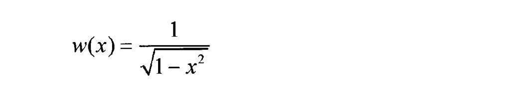
ここにチェビシェフ多項式は解析的に記述できる。n=0,1,2,...の値をとる。
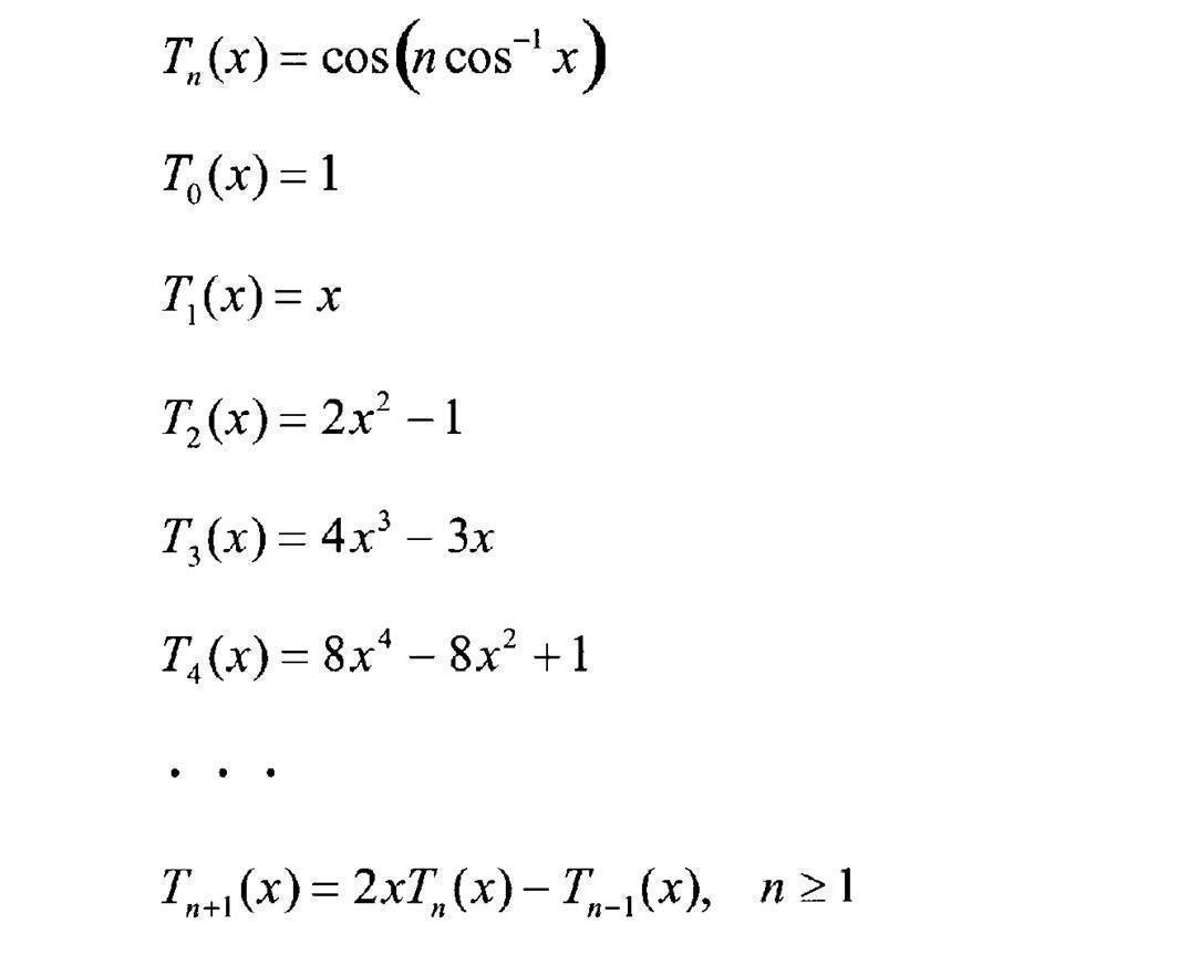
ここで図1にチェビシェフ多項式Tn(x)におけるT1(x),T2(x),T3(x)のグラフを示す。
規格化条件を含めた正確な直交性の関係式は以下で与えられる。
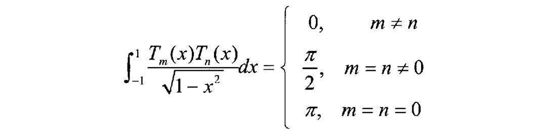
規格化条件を含めた正確な直交性の関係式は以下で与えられる。
チェビシェフ関数の直交性は、分布関数の立ち上がり部と立ち下がり部に極めて密度の高い重点を置いている。すなわち、ヒストグラムのように有限の区間で急激に事象が生じて急激にその事象が終わるような性質の関数系を扱う場合、その関数の形状として立ち上がり部と立ち下がり部が非常に重要な性質を担っており、そこを正確に記述しない限り本当の意味でうまく近似することができないことを示している。
2)テキスチャPDFの場合
球ベッセル関数は1つの次数について取り出すと、[0,a]の区間に存在す根の数によって低周波から高周波までスケーリングされた関数群は根に関して直交性をなすとともに完全系をなす。原点にピークがあるのは0次関数であるので、0次関数の根による一重級数展開を行う。そのとき、テキスチャPDFの分布関数をピークの右区間と左区間の別々に展開をしなければならない。
球ベッセル関数は1つの次数について取り出すと、[0,a]の区間に存在す根の数によって低周波から高周波までスケーリングされた関数群は根に関して直交性をなすとともに完全系をなす。原点にピークがあるのは0次関数であるので、0次関数の根による一重級数展開を行う。そのとき、テキスチャPDFの分布関数をピークの右区間と左区間の別々に展開をしなければならない。
2-1)一重級数展開の場合
基底関数

基底関数
ここで図2に、n=1~5のグラフを示す。
直交性の重み関数

ここに球ベッセル関数は解析的に記述できる。
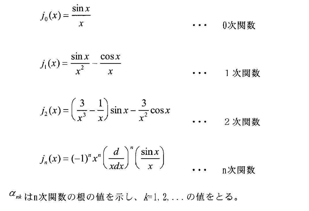

ここで図3に球ベッセル関数のj0(x),j1(x),j2(x)のグラフを示す。
規格化条件を含めた正確な根に関する直交性の関係式は以下で与えられる。

規格化条件を含めた正確な根に関する直交性の関係式は以下で与えられる。
球ベッセル関数は0次関数の場合、原点に最大強度をもつ関数だから、原点に最大度数をもつ分布関数を近似したとき、常に原点の重みを外して、裾野の形を重視する。
ところで、種々のベッセル関数は原点から周辺に向かって光や波が拡散したり、原点に光源のような特異点がある場合の記述に適した関数である。球ベッセル関数は球面座標系における動径成分の波動を記述するのに適しており、円筒座標系のベッセル関数に比べ原点から離れるに従ってその強度の低下が速い。今、扱おうとしているエッジ画像の一次元分布関数は、その急激な強度の低下速度からいって球ベッセル関数の性質に近い。なぜならば、レンズを通して写真が撮られる集光過程を考えても、半球面から降り注いでくる光は球面波であり、それの動径成分は球ベッセル関数で記述され、とくに円筒座標にすべき非等方性の理由が見つからないからである。
球ベッセル関数は、0次関数を用いると常に原点にピークが存在するので、エッジ画像のヒストグラムのように常に原点にピークが現れる性質の分布関数の形状を評価するのに、原点の重みを外して、裾野の性質に焦点を当てるというのは、極めて相性のよい方法となる。それによって、事象の本質との間に線型な関係を生む素地をつくる役割を果たす。
2-2)二重級数展開の場合
球ベッセル関数は、通常動径方向の運動を記述する関数であるので、普通は正の領域で定義されるが、負の領域に拡大定義することによって、異なる次数の関数の間でも直交性が現れるようになる。これは球ベッセル関数には偶数次は偶関数となり、奇数次は奇関数となる性質があるためである。

球ベッセル関数は、通常動径方向の運動を記述する関数であるので、普通は正の領域で定義されるが、負の領域に拡大定義することによって、異なる次数の関数の間でも直交性が現れるようになる。これは球ベッセル関数には偶数次は偶関数となり、奇数次は奇関数となる性質があるためである。
ここで図4に負の領域に拡大定義された球ベッセル関数j0(x)~j5(x)のグラフを示す。
球ベッセル関数の次数に関する直交性

球ベッセル関数の次数に関する直交性
次数に関する直交性と根に関する直交性を合わせて考えれば、分布関数の正の領域と負の領域は同時に展開することができる。根展開に関しては常に完全性を持っていることから、次数と根の二重級数に展開する。差し当たり、非対称性の成分を抽出する奇関数が1つあればよいので、0次の偶関数と1次の奇関数の2つを用いた根展開でよい。

[5]展開係数と力学との対応関係
<問題提起>
展開係数は分布関数のなかで、基底関数に対応する波形及び振動数をもった成分が多いことを意味する。ここで、「展開係数ciそのものは感性特徴量にふさわしいか」という問題がある。
<問題提起>
展開係数は分布関数のなかで、基底関数に対応する波形及び振動数をもった成分が多いことを意味する。ここで、「展開係数ciそのものは感性特徴量にふさわしいか」という問題がある。
<実データにおける展開係数の傾向>
実際に分布関数を展開した係数ciの値は、各々の分布関数の絶対的な形状に直接的に左右されやすい。したがって、値としては画像による変動が極めて大きい。同じ形容詞を付与したもの同士の画像の分布関数について、展開係数を直接比べてみると少しの相関傾向は認められるものの、それ以上にばらつく傾向が強い。仮に同じ形容詞が付与された画像同士で展開係数の統計平均をとる学習を行って、その展開係数をその形容詞に対応するモデルとしようとしても、ほとんどの展開係数がゼロに消滅するか、他の形容詞でも共通の意味のないある定数に収束してしまいそうな傾向である。
実際に分布関数を展開した係数ciの値は、各々の分布関数の絶対的な形状に直接的に左右されやすい。したがって、値としては画像による変動が極めて大きい。同じ形容詞を付与したもの同士の画像の分布関数について、展開係数を直接比べてみると少しの相関傾向は認められるものの、それ以上にばらつく傾向が強い。仮に同じ形容詞が付与された画像同士で展開係数の統計平均をとる学習を行って、その展開係数をその形容詞に対応するモデルとしようとしても、ほとんどの展開係数がゼロに消滅するか、他の形容詞でも共通の意味のないある定数に収束してしまいそうな傾向である。
<力学との対応関係の構築>
ここで以下のような力学と画像系を対応させた仮説を立てる。
ここで以下のような力学と画像系を対応させた仮説を立てる。
力学系:
「各々の粒子の運動状態(運動量pi)が変化しても運動系全体を特徴づける保存量(エネルギーE)が存在する。」
画像系:
「各画像の画素値分布(状態成分ci)が変化しても画像全体の感性を特徴づける不変量(I)が存在するはずである。」
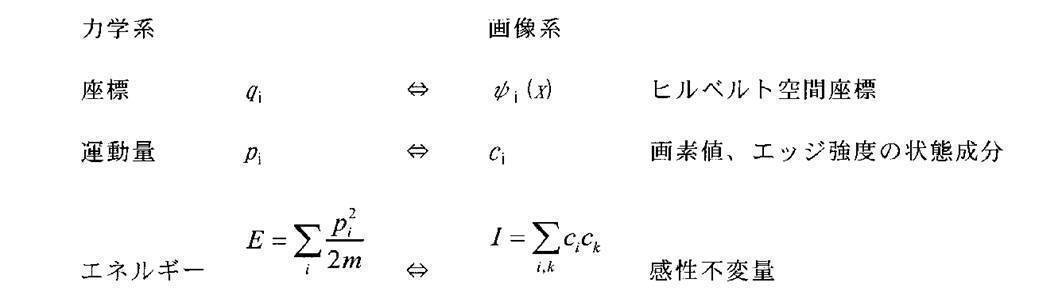
「各々の粒子の運動状態(運動量pi)が変化しても運動系全体を特徴づける保存量(エネルギーE)が存在する。」
画像系:
「各画像の画素値分布(状態成分ci)が変化しても画像全体の感性を特徴づける不変量(I)が存在するはずである。」
画像の信号分布、あるいは外界の視覚野に映った像を人が知覚したとき、そこにある種の感性の「場」のエネルギーのようなものを感じとって、瞬時にその種類の場のエネルギーに対応する脳内の神経状態が励起されて形容詞が想起されるというメカニズムを、この仮説はモデルとして含んでいる。
展開係数の2次形式の和が、分布関数が様々に変化しても、同一の感性を想起させる画像群の分布関数の間で共通に備えた特徴を抽出しうることを意味する。この和をとる操作が、個々の要素の厳密な類似性の要求を緩和し、総体的に類似した特徴群を集約するため、曖昧に形状が似通った特徴を照合する機能を導き出す。
<2次形式と加法性について>
感性不変量が2次形式をとらなければならないとの結論に至った理由には、理論物理学における最小作用の原理に基づく作用関数からの運動方程式の導出過程やハミルトニアンの構築過程における理論的背景とに深く関わっている。すなわち、感性の場の運動方程式の1つの側面が線型微分方程式を満足していると仮定するとき、その作用関数の被積分関数であるラグランジアンには感性の場について2次の表式がくることを要求されるからである。なぜならば、運動方程式は変分原理に基づいて作用積分の一階の全微分がゼロに等しいと置くことによって導かれ、その時に次数を1つ落とすことによって重ね合わせの原理が保たれるからである(文献A1参照)。そして、運動方程式の第1積分である力学的不変量は運動の積分と呼ばれ、運動の間一定の値を保つ。これが感性の場合は、画像の信号分布が変わっても同一の感性を与え続けることに対応すると考える。
感性不変量が2次形式をとらなければならないとの結論に至った理由には、理論物理学における最小作用の原理に基づく作用関数からの運動方程式の導出過程やハミルトニアンの構築過程における理論的背景とに深く関わっている。すなわち、感性の場の運動方程式の1つの側面が線型微分方程式を満足していると仮定するとき、その作用関数の被積分関数であるラグランジアンには感性の場について2次の表式がくることを要求されるからである。なぜならば、運動方程式は変分原理に基づいて作用積分の一階の全微分がゼロに等しいと置くことによって導かれ、その時に次数を1つ落とすことによって重ね合わせの原理が保たれるからである(文献A1参照)。そして、運動方程式の第1積分である力学的不変量は運動の積分と呼ばれ、運動の間一定の値を保つ。これが感性の場合は、画像の信号分布が変わっても同一の感性を与え続けることに対応すると考える。
運動の積分にはエネルギーと運動量と角運動量があり、これらは全て加法性という重要な性質を持っていることが、力学によって明らかにされている(文献A2参照)。また、感性が問題とするような画像の信号分布は、10の6乗から8乗のオーダーの画素数からなる画像とそれらの何百枚、何千枚という画像群からなる統計集団を相手とするので、統計物理学を用いる必要がある。
統計物理学によると相加的な運動の積分の中で、統計平均後に系全体の統計的な性質、すなわち系の統計分布を決めるのはエネルギーだけであるとの結論が導かれている。運動量と角運動量は、単に系全体の一様な並進運動と一様な回転運動だけに帰されて、系の記述には役立たない(文献A3参照)。この事情は、感性を記述するために分布関数から導いた運動量に対応する展開係数ciが、同一感性の画像群の間で統計平均を行うと、意味のない定数に収束する傾向にある事実と符合する。
分布関数fと力学的不変量、すなわちエネルギーの次元を有した2次形式の物理量との対応関係を上記と同じくまとめると、
力学系 画像系
f=f(E) ⇔ I=I(f)
ここでは、観測量である分布関数から感性不変量を導出することになるので、力学系とは逆の表式となる。また、2次形式の感性不変量は、次節で説明するように拡張定義することにより種々の感性を扱えるようにした。
力学系 画像系
f=f(E) ⇔ I=I(f)
ここでは、観測量である分布関数から感性不変量を導出することになるので、力学系とは逆の表式となる。また、2次形式の感性不変量は、次節で説明するように拡張定義することにより種々の感性を扱えるようにした。
こうして、全ての感性不変量は加法性を備え、感性の線型モデルの相加性の要件を満たすことになり、色もテキスチャも構図も共通の土俵で扱えるようになる。すなわち、感性主軸の異なる特徴量が全て相加的に扱えるようになる。なお、構図から導出する感性不変量も同じ指針に基づいて同じ要領で構築するものとする。
なお、上述のように感性不変量を2次形式にする必要があると至った過程には、実験的な試行錯誤を経てきた上で、上述の理論的な背景が内在すると判断したためである。すなわち、実験的に、展開係数の絶対値や比など考えられうる多くの指標を作って試してみても、全く感性との間で感覚に合致するような画像の整列が得られず何度も失敗を繰り返し、2次形式の和の表式によって初めて感性との整合性の高い整列が得られたことに基づく。
[文献A1]ランダウ=リフシッツ理論物理学教程第2巻「場の古典論」(原書第6版、1973年)、第4章「場の方程式」、第27節「電磁場の作用関数」
[文献A2]ランダウ=リフシッツ理論物理学教程第1巻「力学」(増訂第3版、1973年)、第1章「運動方程式」と第2章「保存法則」
[文献A3]ランダウ=リフシッツ理論物理学教程第5巻「統計物理学第1部」(第3版、1976年)、第1章「統計の基礎原理」、第4節「エネルギーの役割」
[6]感性不変量の2次形式表現
<2つの基底状態の合成>
2次形式の感性不変量を作るには、分布関数の形状認識するという視点に立ち返って、2つの基底状態ψi,ψkの合成系によって分布関数fの形状を抽出する。一般に、任意の関数f(α)がn個の基底関数による展開で表されるものとする。
[文献A2]ランダウ=リフシッツ理論物理学教程第1巻「力学」(増訂第3版、1973年)、第1章「運動方程式」と第2章「保存法則」
[文献A3]ランダウ=リフシッツ理論物理学教程第5巻「統計物理学第1部」(第3版、1976年)、第1章「統計の基礎原理」、第4節「エネルギーの役割」
[6]感性不変量の2次形式表現
<2つの基底状態の合成>
2次形式の感性不変量を作るには、分布関数の形状認識するという視点に立ち返って、2つの基底状態ψi,ψkの合成系によって分布関数fの形状を抽出する。一般に、任意の関数f(α)がn個の基底関数による展開で表されるものとする。
f(α)=c1
(α)ψ1
(α)+c2
(α)ψ2
(α)+...+cn
(α)ψn
(α)
群論によれば、合成系の直積で表されるn*n個の基底状態ψiψkは簡約可能な表現で、n(n+1)/2個の対称積とn(n-1)/2個の反対称積で表される2つの基底状態に分割することができる(文献A4参照)。

群論によれば、合成系の直積で表されるn*n個の基底状態ψiψkは簡約可能な表現で、n(n+1)/2個の対称積とn(n-1)/2個の反対称積で表される2つの基底状態に分割することができる(文献A4参照)。
色相面(H)と輝度面(V)と彩度面(C)の各々の分布関数を同じ基底関数を用いて級数展開すると、同一色面内の分布関数の形状の特徴は、対称積の基底関数が作る波形の展開成分によって測ることができ、色面間の分布関数の形状の特徴は、対称積の基底関数が作る波形の展開成分とともに、反対称積の基底関数が作る波形の展開成分によっても測ることができる。これらの合成系の波形による展開成分は、合成前の基底状態が相互に直交することが保証されているから、合成系の基底状態による展開係数は、対称積と反対称積の形をした行列要素として表現できる。
感性不変量を行列のシュプール(跡)をとることによって定義する。ただし、通常シュプールは対角要素の和のみを指すが、ここでは行と列の位置が一定の量子数の差だけを保った非対角成分同士の斜め方向の和をとる新たな拡張型のシュプールを定義する。これによって、一定の量子数の差を保った2つの基底状態による合成波形の成分が、分布関数のなかにどれだけの割合で存在しているかが、作りうる全ての合成波形に渡って総和をとった状態で検出することができる。色面の異なる2つの分布関数の間では、一定の量子数の異なった基底状態の組み合せが、どの程度の割合で存在しているかということを、その組み合わせの対称状態と反対称状態の2種類の合成波形で評価していることになる。

ここに、ciを色ヒストグラムのチェビシェフ展開係数にとった場合は、Ii=Fiとなり、ciをテキスチャPDFの球ベッセル展開係数にとった場合は、Ii=Giとなる。ただし、番号iは対称、反対称の区別なく、複数個求まった不変量の要素に対して順番に割り当てるものとする。
ここで上記定義の感性不変量を、電磁場における場の不変量と比較してみることにする。文献A5によると、電場Eと磁場Hのローレンツ変換に対する不変量として、真のスカラーと擬スカラーの2種類が存在する。
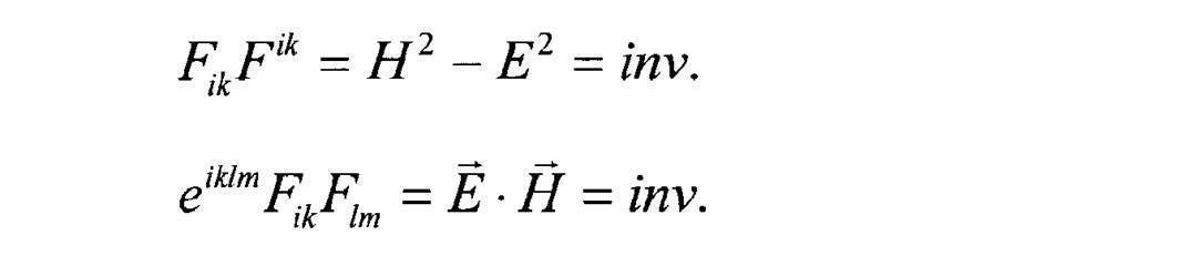
両者とも4次元の電磁場テンソルFikの2次形式のシュプールで求められ、後者には完全反対称な単位テンソルeiklmが付随し、前者にはそれが付随しない。ただし、テンソルに関する和の記号は、アインシュタイン規約によって省略されている。
したがって、1つの画像から別の画像に移っても同一の感性を与える感性不変量は、電磁場における1つの基準系から他の基準系に変換したときの場の不変量と極めて似た構成になる。前節では、感性不変量を運動エネルギーに対応させて議論したが、むしろ2種類にとどまらない複数種類の「感性場」というものが存在し、場のエネルギーが伝わってくると考えた方が素直である。また、電磁場の構成要素は時間と空間の4次元であるが、感性の構成要素には少なくとも分布関数の記述に必要な次数以上の要素が存在していると推測される。しかし、人間の脳の神経回路が成育過程の学習の中で、これらの感性場に対して、場に誘起される電気信号回路が構築される、あるいはエネルギー的に瞬時に励起される神経回路のエネルギー準位を獲得していくというのは自然な考えである。
[文献A4]Landau and Lifshitz, Course of Theoretical Physics, Volume 3 "Quantum Mechanics (Non-Relativistic Theory)," (Third revised edition, 1977), Chapter 12 "The Theory of Symmetry," Section 94 "Representations of groups."
[文献A5]ランダウ=リフシッツ理論物理学教程第2巻「場の古典論」(原書第6版、1973年)、第3章「場のなかの電荷」、第23節「電磁場テンソル」、第24節「ローレンツ変換」、及び第25節「場の不変量」
[第1の実施形態]
(色ヒストグラムのヒルベルト空間表現と感性不変量の線形和)
以下、図面を参照して、第1の実施形態に係る画像分類装置の説明を行う。図5は、実施の形態に係る画像分類装置を示すブロック図である。ここで画像分類装置は、パーソナルコンピュータ10により実現される。パーソナルコンピュータ10は、デジタルカメラや他のコンピュータと接続され、デジタルカメラや他のコンピュータから画像データの提供を受け、またはメモリーカードスロットに装着されたメモリカードから画像データの提供を受け、ハードディスク装置(図示せず)へ蓄積する。パーソナルコンピュータ10は、蓄積された画像データに対して以下に説明する画像分類処理を行う。
パーソナルコンピュータ10に対する画像分類プログラムのローディングは、プログラムを格納したCD-ROMなどの記憶媒体から行ってもよいし、ネットワーク12などを介して行ってもよい。ネットワーク12を介する場合には、サーバ14に接続されているハードディスク装置16から読み出したプログラムをローディングする。パーソナルコンピュータ10は、CPU及びCPUにより制御される周辺回路から構成され、CPUがインストールされたプログラムに基づいて図6のフローチャートに示す画像分類処理を行う。
<検索対象画像への処理>
1.マンセルHVC色空間への変換(図6ステップS1)
入力画像を人間の知覚的な均等色性が高いマンセル色空間へ変換する。マンセル色空間は、色相Hが一周100度で分割され、輝度Vが0~10のレベルに、彩度Cが0~25程度のレベルに分布するように刻まれた色空間で、Vの色差1に対してCの色差2が同等の色差として知覚する等歩度性を満たすように設計された色空間である。その内のCの値が1以下の領域とVの値が0.5以下、及び9.5以上の領域がN(ニュートラル色相)と定義されている。RGB空間で表された色空間からHVC色空間へはXYZ空間への変換を介して近似的に数式変換できる。これは、均等色空間の1つであるL*a*b*ないしはL*C*H*の定義を利用して、その均等色性の不十分であるところを修正する式を導入することによって実現されている。
入力画像が例えば出力ガンマ特性の掛かったsRGB色空間で表された画像である場合、まず、線形階調に戻した後、XYZ空間へsRGB規格に従って変換する。

第1の実施形態では、色相面はN(ニュートラル)の分離を行った面を用意するものとする。
2.色の一次元分布関数の作成(図6ステップS2)
HVC面各々のヒストグラムを作成する。ヒストグラムのビン数はH,V,C共に200程度に設定するとよい。このとき、色相面はNの分離を行った面を使う。したがって、H面のヒストグラムは、色相環で積分してもNに分類された面積率は含まれないことになる。通常Nは色相環ではランダムに分布するから、乱雑に一様なオフセット状の分布が色相面のヒストグラムから除外され、本来の有彩色のヒストグラム形状が残ることになる。便宜上、画素数でヒストグラムの値を規格化しておけば、画素値の確率密度を表す一次元分布関数になる。模式的に作成した分布関数を次のように表す。
f(H), f(V), f(C)
3.分布関数のヒルベルト空間表現(図6ステップS3)
3-1.変数変換
ヒストグラムの横軸の分布域を[a,b]、縦軸の分布域を[fa,fb]とすると、横軸を[-1,1]に、縦軸を[-1,1]に収まる区間に変数変換を行う。この節の中だけ便宜的に、横軸の変数をxからyへ、縦軸の変数をfxからfyへ変換して表記すると、変換式は以下のようになる。
横軸の変数変換:y={x-(b+a)/2}/{(b-a)/2}
縦軸の変数変換:fy={fx-(fb+fa)/2}/{(fb-fa)/2}
色相面のヒストグラムの分布域は色相環のため、始まりの区切り点を設け、そこから一周して同じ点に戻る分布域を設定する。始まり点aは固定点ではなく、各々の画像毎に分布関数の密度が最小となる点を探して、そこに区切り点を入れるものとする。
縦軸の変数変換:fy={fx-(fb+fa)/2}/{(fb-fa)/2}
色相面のヒストグラムの分布域は色相環のため、始まりの区切り点を設け、そこから一周して同じ点に戻る分布域を設定する。始まり点aは固定点ではなく、各々の画像毎に分布関数の密度が最小となる点を探して、そこに区切り点を入れるものとする。
縦軸の変数変換の定義の仕方によって、以下に示す級数展開係数にある定数要因が加わる。これは概論説明で行ったように展開係数が運動量に相当すると考えると、画像群の統計平均によって残留するその定数因子は、画像群系全体のヒルベルト空間座標系の選択の仕方によって系全体の一様な並進運動となって残ることに相当する。
3-2.チェビシェフ多項式による級数展開
上述の変数変換がなされた横軸の分布域をH,V,Cに関係なくxで表す。HVCの各分布関数をN個の次数のチェビシェフ関数で展開する。
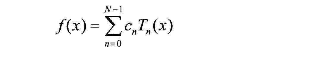
上述の変数変換がなされた横軸の分布域をH,V,Cに関係なくxで表す。HVCの各分布関数をN個の次数のチェビシェフ関数で展開する。
展開係数cnは、基底関数の直交性を利用して、以下の式で求められる。

ただし、n=0のときは特別にc0=c0/2とする。
ここで変数変換を導入する。

こうすると展開係数は以下のように簡略に求まる。

色ヒストグラムのビンの数が200程度のときは、展開の次数をN=50程度に設定するとよい。
4.感性不変量の生成(図6ステップS4)
2つのチェビシェフ基底関数の合成系によって、H,V,Cヒストグラムの分布関数の形状を抽出する。すなわち、HVCの分布関数がとる構造によって現れる感性を特徴量として抽出する。
2つのチェビシェフ基底関数の合成系によって、H,V,Cヒストグラムの分布関数の形状を抽出する。すなわち、HVCの分布関数がとる構造によって現れる感性を特徴量として抽出する。
展開係数の2次形式によって作られる行列要素に対して、一定の量子数の差を持つ行列要素のシュプールによって感性不変量を定義する。量子数差mは対称状態の場合、m=0,1,2,...,N/2まで定義でき、反対称状態の場合、m=1,2,...,N/2-1まで定義できる。量子数の差が0,1,2までの作成例を示す。ここに、1つの例外を除いては、不変量の値が全て[-1,1]に収まるように規格化して定義する。また、和の範囲がk=0,1,...,N-1の範囲をはみ出した場合は、k=N-1の次にk=0が環状につながっているものとして扱う。
同じ色面内の基底関数の合成系による評価

異なる色面間の基底関数の合成系による評価
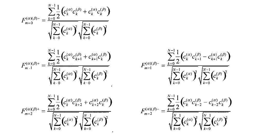
プラス記号のついた不変量は、画像の分布関数の中に占める、合成系の対称状態による波形の符号付きの存在割合を示し、マイナス記号のついた不変量は、画像の分布関数の中に占める、合成系の反対称状態による波形の符号付きの存在割合を示す。
不変量の値がゼロに近ければその合成波形の成分が全く存在しないということを意味し、+1に近ければその合成波形の形のままの成分が多く存在していることを意味し、-1に近ければ合成波形の符号を反転させた波形の成分が多く存在していることを意味する。例として、Fm=2 (α)(α)+のシュプールをとる対象の1つの成分である、対称状態の合成波T1T3とT2T4の波形図(図7参照)を示す。
別の色面間で量子数差がゼロと異なる感性不変量が有意な値を示すとき、ある色面の分布関数と別の色面の分布関数は常に何らかの特有の形状差を伴っているといえる。その反対に、別の色面間で量子数差がゼロの感性不変量が有意な値を示すとき、2つの色面の分布関数の形状は極めて似ているといえる。
Fm=0 (α)(α)+だけは規格化ができない。分布関数の値の区間を[-1,1]に変数変換しているので、実際の値はゼロに近い値、あるいは0.4程度から約1.5程度までの値をとる。この値が意味する内容は、値が大きいほど、分布関数の中である基底状態に一極集中して表現される割合が高く、値が小さいほどいろんな基底状態に分散して表現される割合が高いということを示す。Fm≠0 (α)(α)+についても同様に、値の絶対値が大きければ合成系の基底状態の内、ある1つの合成波形への一極集中度が高く、値の絶対値が小さければ合成系の基底状態の多くに分散して表現されるか、もしくは、この合成系の基底状態で表される波形成分はあまり存在していないことを意味する。
対称状態と反対称状態は互いに共役な関係にある。同じ量子数差の対称積と反対称積の感性不変量について、その不変量に関する画像群の整列度を調べてみると、対称積では値が零付近に集まって何の感性をもっているのか不明であった画像群が、反対称積ではその指標の分布の中の両端部に現れる。また、その逆も真で、反対称積の指標では不明な画像群が対称積の指標では画像分布の両端部に現れる。この事実は数式的に次のように考えれば当然の帰結である。すなわち、対称積の値がゼロのときci
(α)ck
(β)=-ck
(α)ci
(β)であるので、反対称積の値ci
(α)ck
(β)-ck
(α)ci
(β)=2ci
(α)ck
(β)=-2ck
(α)ci
(β)となって±のどちらかにもっとも大きな値をとりやすい。
5.形容詞判別指標の作成(図6ステップS5)
5-1.感性不変量の線形結合
ある感性形容詞(i)を検索するための指標として、感性不変量の加法性の性質を利用して、各々の感性不変量を線形結合した新たな指標Qiを作成する。指標Qiが表しうる形容詞は、1つの形容詞だけではなく、正反対の性質の形容詞を備えた一対の形容詞であるものとする。
Qi=α1F1+α2F2+...
ここで、Qiは再度[-1,1]の範囲の指標となるように、線型結合パラメータαiの値を規格化する。
5-2.検索対象形容詞のパラメータ設定
所定の形容詞に対応する線形結合パラメータを事前に学習しておき、そのモデル・パラメータを設定する。
5-1.感性不変量の線形結合
ある感性形容詞(i)を検索するための指標として、感性不変量の加法性の性質を利用して、各々の感性不変量を線形結合した新たな指標Qiを作成する。指標Qiが表しうる形容詞は、1つの形容詞だけではなく、正反対の性質の形容詞を備えた一対の形容詞であるものとする。
Qi=α1F1+α2F2+...
ここで、Qiは再度[-1,1]の範囲の指標となるように、線型結合パラメータαiの値を規格化する。
5-2.検索対象形容詞のパラメータ設定
所定の形容詞に対応する線形結合パラメータを事前に学習しておき、そのモデル・パラメータを設定する。
6.画像分類処理(図6ステップS6)
形容詞判別指標に基づいて、画像を分類する。入力する画像データベース群に対して各々の画像について、形容詞判別指標Qiを計算し、Qiの値の大きさ順に並び替える。判別指標Qiに対して画像群の度数分布は、ガウス分布やポアッソン分布のような形をするので、両端で他の画像群よりも統計的に有意なレベルでその形容詞判別指標に対して特異性を示す画像を提示する。
形容詞判別指標に基づいて、画像を分類する。入力する画像データベース群に対して各々の画像について、形容詞判別指標Qiを計算し、Qiの値の大きさ順に並び替える。判別指標Qiに対して画像群の度数分布は、ガウス分布やポアッソン分布のような形をするので、両端で他の画像群よりも統計的に有意なレベルでその形容詞判別指標に対して特異性を示す画像を提示する。
実際にどのような感性を与える画像が抽出されるか具体例を示す。最も単純な線形結合は、1つの感性不変量に対してのみ係数パラメータが有限で、その他は全て零となる場合である。それらの各々の性質についてのみ示す。複数の係数パラメータが残るときの決め方は、後述のモデル学習の欄で説明する。
実際にこのようにして物理現象の記述がしやすいヒルベルト空間に投影され、さらに画像の信号分布の変化に対して不変に作用し続け、相加的な性質を備えた2次形式の感性不変量からは、色彩心理学で一般性のある高次の形容詞対(文献C1参照)と極めて深い関連性と線型性を示すことが実験的に確認することができた。その深い関連性を示すために、以下に各々の感性不変量から整列することのできる形容詞対の用語の例を記載する。
また、同じ型の感性不変量で量子数差の値を変えたもの同士の間では、感性軸が段々と遷移していく様子が実験的に認められた。これは形容詞の2面性の性質と非常に相性のよい記述方法になっている。すなわち、形容詞には例えば「賑やかな」という大分類に対して、「華やかな」や「派手な」や「騒がしい」といった微細分類の同次表現性が存在し、その細やかな分類能力も感性検索には不可欠となる。
有効な量子数差の範囲は、行列要素の非対角成分が対角成分のとりうる値に対して、すなわち±1に比べて相対的に小さくなるところでは、もはや意味のある感性分類能力がないと考えるのが適当である。すなわち、行列要素のシュプールである感性不変量の値の分布範囲が広いと、感性との対応性が高い整列が得られるが、その分布範囲が小さくなるともはや対応関係は見えてこない。これは実験的にも確認している。
[文献C1]日本色彩学会編、色科学講座第1巻「カラーサイエンス」(朝倉書店、2004年)、第3章「色彩の心理学」、第3.2節「感覚・知覚・認知の測定法」、表3.4「色彩のイメージ測定によく使用される形容詞対」及び第3.4節「色彩の認知」、表3.13「日米学生の色に対する因子分析の比較」
以下に具体例を示す。

以下に具体例を示す。
これは、3つの色面の各々で生成した感性不変量の相加平均である。この感性不変量からは「静的-動的」という形容詞対の感性画像が整列する。「静的な」画像には遠景の風景写真で時が一瞬止まったような画像が集まる。一方の「動的な」画像にはお祭りで多数の人物が踊っていたりする写真や都会の喧騒が伝わってくる写真が集まる。
図8に画像分布の両端近くに位置する画像のHVC面の色ヒストグラム形状の例を示す。「静的な」画像の色ヒストグラムはH,V,C面のいずれもが1つの基底関数の状態成分に集まった1つのバンド構造のような形状をして集団的であるのに対し、「動的な」画像ではH,V,C面の各々で多くの複雑なピーク形状を有し、単純な波形では記述できそうにもないヒストグラム構造をしていて分散的である。

この感性不変量からは「引き締まった-開放的な」という形容詞対の感性画像が整列する。「引き締まった」画像には陰影を多くもつ画像が集まる。一方の「開放的な」画像には全体的に少し明るさと空間的な広がりをもった画像が多く集まる。
図9に画像分布の両端近くに位置する画像のHVC面の色ヒストグラム形状の例を示す。「引き締まった」画像の色ヒストグラムは、VC間で極めて形状の類似性が高い。一方の「開放的な」画像の色ヒストグラムはV面とC面で全く異なる形状をしている。

この感性不変量からは「興奮した-沈静した」という形容詞対の感性画像が整列する。この形容詞対は対称積から導き出された「引き締まった-開放的な」の形容詞対と共役な関係にあると位置づけられる。「興奮した」画像には色が派手な銀杏やもみじの木や葉からなる紅葉の写真であったり、風景写真の夕方の一瞬のピンク色の輝きを捉えた写真や雲が湧き立つような一瞬の動きを捉えた写真が多く集まる。一方の「沈静した」画像には動きが完全に止まった瞬間を捉え、更に深い色を兼ね備えた写真が集まる。
<感性形容詞のモデル学習>
感性不変量の値は、画像の分布関数の観測量から一意的に決まるものである。事前学習することによって形容詞との対応関係をとるのに必要なのは、各々の形容詞について線形結合パラメータを決めることである。
感性不変量の値は、画像の分布関数の観測量から一意的に決まるものである。事前学習することによって形容詞との対応関係をとるのに必要なのは、各々の形容詞について線形結合パラメータを決めることである。
1)最小二乗法
一人もしくは複数人がある形容詞に対して、その印象を備える画像を学習データ用の画像群の中から選択する。それの再現性を測る二乗誤差の関数を導入し、線形結合パラメータを未知であるとして、1つ1つのパラメータを偏微分して極小点を求めていく形で、各々の結合パラメータを決める。これは最小自乗法による係数のフィッティングである。
一人もしくは複数人がある形容詞に対して、その印象を備える画像を学習データ用の画像群の中から選択する。それの再現性を測る二乗誤差の関数を導入し、線形結合パラメータを未知であるとして、1つ1つのパラメータを偏微分して極小点を求めていく形で、各々の結合パラメータを決める。これは最小自乗法による係数のフィッティングである。
2)画像分布のガマットにおける位置関係からの決定
ある画像の分布関数から複数の感性不変量を生成したとき、その画像が画像データベース群全ての画像についても求めた感性不変量のなかで、どの位置を占めていているかということは、その画像が発する感性そのものの性質を表している。すなわち、1つ1つの感性不変量に対する画像群の分布の端の境界線を、自然画像の信号分布がとりうるガマットと見なすことができる。このガマットの端に位置している画像は、その不変量に対しては極めて重要な信号を発していると考えてよく、真ん中に位置している画像はその不変量に対して無関係な性質であるといえる。したがって、そのガマット内におけるその画像が存在している位置をそのまま、線型結合パラメータの値として[-1,1]の範囲の数値を設定すればよい。ただし、全線型結合パラメータの間の規格化は最後に行うものとする。
ある画像の分布関数から複数の感性不変量を生成したとき、その画像が画像データベース群全ての画像についても求めた感性不変量のなかで、どの位置を占めていているかということは、その画像が発する感性そのものの性質を表している。すなわち、1つ1つの感性不変量に対する画像群の分布の端の境界線を、自然画像の信号分布がとりうるガマットと見なすことができる。このガマットの端に位置している画像は、その不変量に対しては極めて重要な信号を発していると考えてよく、真ん中に位置している画像はその不変量に対して無関係な性質であるといえる。したがって、そのガマット内におけるその画像が存在している位置をそのまま、線型結合パラメータの値として[-1,1]の範囲の数値を設定すればよい。ただし、全線型結合パラメータの間の規格化は最後に行うものとする。
前述のように1つの形容詞に対して複数の画像が学習用として選択されているとき、選択された画像群について、各々の感性不変量のガマット内で単純に統計平均した座標位置を、その形容詞に対する線形結合パラメータの学習結果とすればよい。もしある感性不変量に対して選択された画像群がバラバラに散らばっているときは統計平均によってパラメータαiの値はゼロに近づき、その形容詞にとってその感性不変量は無関係であるということになる。その反対に、選択された画像群で同じ方向に集まってくる場合は、統計平均してもパラメータαiには有意な値が残り、その感性不変量はその形容詞にとって重要である。こうして、ある形容詞にとって特別な働きをする感性不変量が極めて単純に導き出される。なお、上述のモデル学習の方法は以下に説明する全ての実施形態で共通に使用することができる。
[第2の実施形態]
(テキスチャPDFのヒルベルト空間表現と感性不変量の線形和)
次に、第2の実施形態に係る感性不変量の生成について説明する。なお、第2の実施形態においては、第1の実施形態における感性不変量の生成方法を以下の方法に変更した。
(テキスチャPDFのヒルベルト空間表現と感性不変量の線形和)
次に、第2の実施形態に係る感性不変量の生成について説明する。なお、第2の実施形態においては、第1の実施形態における感性不変量の生成方法を以下の方法に変更した。
<検索対象画像への処理>
1.マンセルHVC色空間への変換
色相面はNの分離を行わない面を用意するものとする。N領域の色相面は、色相面内でランダムノイズのように振る舞うことになるが、以下のエッジ抽出過程ではそれが他の有彩色の色相と異なる特徴として検知される役割を果たす。
1.マンセルHVC色空間への変換
色相面はNの分離を行わない面を用意するものとする。N領域の色相面は、色相面内でランダムノイズのように振る舞うことになるが、以下のエッジ抽出過程ではそれが他の有彩色の色相と異なる特徴として検知される役割を果たす。
色相環における一次元座標の採り方は、マンセル色相環の原点である赤色を始点に一周して終点を赤紫を経てもう一度赤色にしてもよいが、より望ましくは第1の実施形態と同様に各々の画像で色相の分布度数が最小となる点に切り込みを入れてそこに始点と終点を設定するとよい。そうすると色相環の分断によって信号強度が両端に振れ、その色面内でエッジ抽出したときのエッジ成分の過大評価による悪影響が最小限に抑えられるためである。
2.エッジ画像の作成
2-1.多重解像度変換とエッジ抽出
1)ウェーブレット変換
ウェーブレット変換を用いて多重解像度表現された周波数空間に射影して、HVC各色面の高周波のエッジ成分を抽出する。ここではエッジ成分として、ウェーブレット分解された高周波サブバンドLH,HL,HHをそのまま使うものとする。この様子を模式的に書けば、解像度M段まで分解するとき

となる。なお、LL成分は順次解像度の低い高周波サブバンドに分解されていくので、最終的に残るLL成分は最低解像度のみとなる。ウェーブレット変換としては、例えば以下のような5/3フィルタなどを用いる。
2-1.多重解像度変換とエッジ抽出
1)ウェーブレット変換
ウェーブレット変換を用いて多重解像度表現された周波数空間に射影して、HVC各色面の高周波のエッジ成分を抽出する。ここではエッジ成分として、ウェーブレット分解された高周波サブバンドLH,HL,HHをそのまま使うものとする。この様子を模式的に書けば、解像度M段まで分解するとき
となる。なお、LL成分は順次解像度の低い高周波サブバンドに分解されていくので、最終的に残るLL成分は最低解像度のみとなる。ウェーブレット変換としては、例えば以下のような5/3フィルタなどを用いる。
<ウェーブレット変換:Analysis/Decompositionプロセス>
ハイパス成分:d[n]=x[2n+1]-(x[2n+2]+x[2n])/2
ローパス成分:s[n]=x[2n]+(d[n]+d[n-1])/4
上記定義の1次元ウェーブレット変換を、横方向と縦方向に独立に2次元分離型フィルタ処理を行うことによって、ウェーブレット分解する。係数sをL面に集め、係数dをH面に集める。
ハイパス成分:d[n]=x[2n+1]-(x[2n+2]+x[2n])/2
ローパス成分:s[n]=x[2n]+(d[n]+d[n-1])/4
上記定義の1次元ウェーブレット変換を、横方向と縦方向に独立に2次元分離型フィルタ処理を行うことによって、ウェーブレット分解する。係数sをL面に集め、係数dをH面に集める。
2)ラプラシアン・ピラミッド
さらに多重解像度変換の別の方法として、ウェーブレット変換以外にラプラシアン・ピラミッドを使う方法もある。ラプラシアン・ピラミッドを作る場合は、一旦縦横(1/2)*(1/2)の縮小画像を作ってバイリニア変倍により元の大きさの画像に戻し、縮小前の画像との差分をとることによりその解像度の高周波画像(ラプラシアン成分)を得る。なお、縮小画像を作る前にエイリアジングを防ぐための平滑化を行ってもよい。これを次々に繰り返せば、高周波画像が連なったラプラシアン・ピラミッドができる。ウェーブレット変換の場合と同じく、最低解像度に1つだけ低周波画像(ガウシアン成分)が残る。
こうして多重解像度変換によって生成された高周波バンドの信号値のヒストグラム(確率密度関数と呼ばれ、PDFで略される)が、ガウス分布やラプラス分布をすることが文献D1に記載されている。一般に、PDFの分布形状は対称なGeneralized Gaussianで近似できる。
多重解像度変換の段数Mの値は、各バンドのPDFのヒストグラムが荒れない程度の画素数を有するところまで分解するとよい。例えば、Quad VGAサイズ(1280x960)の画像に対しては5段程度、QVGAサイズ(320x240)の画像に対しては3段程度、2000万画素の画像に対しては7段程度にするとよい。
なお、図10は4段のウェーブレット変換によるサブバンド分割の様子を示す図である。たとえば、第1段のウェーブレット変換では、実空間の画像データに対し、まず横方向にすべての行についてハイパスの成分及びローパス成分のデータを抽出する。その結果、横方向に半分の画像数のハイパス成分及びローパス成分のデータが抽出される。それを、たとえば実空間の画像データがあったメモリ領域右側にハイパス成分、左側にローパス成分を格納する。
なお、図10は4段のウェーブレット変換によるサブバンド分割の様子を示す図である。たとえば、第1段のウェーブレット変換では、実空間の画像データに対し、まず横方向にすべての行についてハイパスの成分及びローパス成分のデータを抽出する。その結果、横方向に半分の画像数のハイパス成分及びローパス成分のデータが抽出される。それを、たとえば実空間の画像データがあったメモリ領域右側にハイパス成分、左側にローパス成分を格納する。
次に、メモリ領域右側に格納されたハイパス成分及び左側に格納されたローパス成分のデータに対して、それぞれ縦方向にすべての列について、ハイパス成分及びローパス成分のデータを抽出する。その結果、メモリ領域右側のハイパス成分及び左側のローパス成分のそれぞれから、さらにハイパス成分及びローパス成分のデータが抽出される。それらを、それぞれのデータがあったメモリ領域下側にハイパス成分、上側にローパス成分を格納する。
その結果、横方向にハイパス成分として抽出されたデータから縦方向にハイパス成分として抽出されたデータをHHと表し、横方向にハイパス成分として抽出されたデータから縦方向にローパス成分として抽出されたデータをHLと表し、横方向にローパス成分として抽出されたデータから縦方向にハイパス成分として抽出されたデータをLHと表し、横方向にローパス成分として抽出されたデータから縦方向にローパス成分として抽出されたデータをLLと表す。ただし、縦方向と横方向は独立であるので、抽出の順序を入れ替えても等価である。
次に、第2段のウェーブレット変換では、第1段のウェーブレット変換で横方向にローパス成分として抽出されたデータから縦方向にローパス成分として抽出されたデータLLに対し、同様にハイパス成分及びローパス成分の抽出を行う。これを4段まで繰り返し行うと図10のようになる。
[文献D1]Michael J. Gormish, "Source coding with channel, distortion, and complexity constraints," Doctor thesis, Stanford Univ., March 1994, Chapter 5: "Quantization and Computation-Rate- Distortion."
2-2.多重解像度統合
上述のようにして抽出された高周波サブバンドは、各解像度スケールにおけるエッジ、テキスチャ、コントラストに関する情報を表している。これらの情報を統括的に扱うため、高周波サブバンドのみによる多重解像度逆変換を行い、エッジ統合を行なう。すなわち、最低解像度の低周波サブバンドLLMを除外し、それらの値を全て零に設定した後に、残りの高周波サブバンドを順次逆ウェーブレット変換を行なう。この様子を模式的に書くと、入力画像と同じ解像度を持つ統合エッジ成分をEとして、以下のような式になる。

2-2.多重解像度統合
上述のようにして抽出された高周波サブバンドは、各解像度スケールにおけるエッジ、テキスチャ、コントラストに関する情報を表している。これらの情報を統括的に扱うため、高周波サブバンドのみによる多重解像度逆変換を行い、エッジ統合を行なう。すなわち、最低解像度の低周波サブバンドLLMを除外し、それらの値を全て零に設定した後に、残りの高周波サブバンドを順次逆ウェーブレット変換を行なう。この様子を模式的に書くと、入力画像と同じ解像度を持つ統合エッジ成分をEとして、以下のような式になる。
この統合段階において、階層の異なるエッジ、テキスチャ、コントラストの情報が空間的な位置関係を考慮して別の階層へ伝達されることになる。なお、ラプラシアン・ピラミッドを用いた場合は、最低解像度のガウシアン面を零に設定し、残りのラプラシアン面を逐次統合することになる。
3.統合エッジの一次元分布関数の作成
HVC各色面から抽出された統合エッジ画像のヒストグラム(PDF)を作成する。ヒストグラムのビン数はH,V,C共に、原点を挟んで-128~128程度に設定するとよい。ただし、HVC各色面が200ビン程度の階調で表されているものとする。
HVC各色面から抽出された統合エッジ画像のヒストグラム(PDF)を作成する。ヒストグラムのビン数はH,V,C共に、原点を挟んで-128~128程度に設定するとよい。ただし、HVC各色面が200ビン程度の階調で表されているものとする。
PDFはエッジ強度のヒストグラムであるので、正と負に同程度の度数積分面積をもつ原点をピークとする分布になる。一般に、解像度間で無相関のメモリレス・ソースである場合、各階層で対称なPDF分布形状をしていたものは、統合してもそのまま対称なPDF分布形状となって統合される。しかしながら、解像度間で相関がある場合、その相関の様子がPDF分布の形状という形で投影されうる。
このように各々の高周波サブバンド面のPDFは、通常「一般化されたガウシアン:exp(-|x|α)」に近似できるが、逐次統合したエッジ面には空間的なコントラストの相関が反映されて、非対称性を含めて多様な形状に変化する。
このような統合エッジのPDF分布の特徴的な形状は、最低解像度からおよそ3段分ぐらいのエッジ成分を統合するとほぼその形が現れてくることが実験的に確認された。したがって、もし簡略に済ませたいような場合は、最後の実解像度まで統合しなくても、統合途中段階のPDF分布形状を評価するようにしてもよい。
便宜上、画素数でヒストグラムの値を規格化しておけば、画素値の確率密度を表す一次元分布関数になる。模式的に作成した分布関数を次のように表す。ラプラシアン記号△を用いたのは、統合エッジ画像が元画像の画素値の2次微分の側面を記述しているからである。
f(△H), f(△V), f(△C)
4.分布関数のヒルベルト空間表現
統合エッジ画像の分布関数を球ベッセル関数で級数展開し、展開係数によって形状を評価できるようにする。第2の実施形態では、右展開と左展開を個別に行うが、後述する第3の実施形態では左右同時展開を行う。そのとき、第2の実施形態では、0次の球ベッセル関数の根による展開を行う。展開区域の最外郭点を固定して、その中に含まれる根の数を増やすことが周波数成分の高い基底関数を生むことに対応する。
f(△H), f(△V), f(△C)
4.分布関数のヒルベルト空間表現
統合エッジ画像の分布関数を球ベッセル関数で級数展開し、展開係数によって形状を評価できるようにする。第2の実施形態では、右展開と左展開を個別に行うが、後述する第3の実施形態では左右同時展開を行う。そのとき、第2の実施形態では、0次の球ベッセル関数の根による展開を行う。展開区域の最外郭点を固定して、その中に含まれる根の数を増やすことが周波数成分の高い基底関数を生むことに対応する。
4-1.変数変換
ヒストグラムのピークから右側の部分について、横軸の分布域を[a,b](a<b)、縦軸の分布域を[fa,fb]とする。横軸を[0,1]に、縦軸を[0,1]に収まる区間に変数変換を行う。ヒストグラムのピークから左側の部分についても同様に、横軸の分布域を[b,a](b<a)、縦軸の分布域を[fa,fb]とし、同様な変換を行う。通例a~0、fa~0の値をとる。この節の中だけ便宜的に、横軸の変数をxからyへ、縦軸の変数をfxからfyへ変換すると表記すると、変換式は以下のようになる。
横軸の変数変換:y=|x-a|/|b-a|
縦軸の変数変換:fy=(fx-fa)/(fb-fa)
4-2.球ベッセル関数の根による級数展開
上述の変数変換がなされた横軸の分布域を△H,△V,△Cに関係なくxで表す。HVC各色面の分布関数をN個の0次の球ベッセル関数の根による基底関数で展開する。ここで用いる記号aの意味は前述までと異なり、分布域の展開対象となる最外郭点を意味する。

ヒストグラムのピークから右側の部分について、横軸の分布域を[a,b](a<b)、縦軸の分布域を[fa,fb]とする。横軸を[0,1]に、縦軸を[0,1]に収まる区間に変数変換を行う。ヒストグラムのピークから左側の部分についても同様に、横軸の分布域を[b,a](b<a)、縦軸の分布域を[fa,fb]とし、同様な変換を行う。通例a~0、fa~0の値をとる。この節の中だけ便宜的に、横軸の変数をxからyへ、縦軸の変数をfxからfyへ変換すると表記すると、変換式は以下のようになる。
横軸の変数変換:y=|x-a|/|b-a|
縦軸の変数変換:fy=(fx-fa)/(fb-fa)
4-2.球ベッセル関数の根による級数展開
上述の変数変換がなされた横軸の分布域を△H,△V,△Cに関係なくxで表す。HVC各色面の分布関数をN個の0次の球ベッセル関数の根による基底関数で展開する。ここで用いる記号aの意味は前述までと異なり、分布域の展開対象となる最外郭点を意味する。
展開係数cnは、基底関数の直交性を利用して、以下の式で求められる。

ここに、αnmはn次関数のm番目の零点の値を意味する。

0次関数の根の場合は、解析的に与えることができる。
α0m=πm, m=1,2,3,...
したがって、級数展開に用いた0次関数のm番目の基底関数は、[0,a]の区間内にm個の零点(根)が存在する。すなわち、0次の球ベッセル関数の最初の零点の位置にaを設定したものをその次数における最低周波数の基底関数とし、その関数を原点方向に向かって縮め、2番目の零点がaの位置に来たときに止め、それをその次数における2番目に周波数の低い基底関数とし、これを次々に繰り返して、分布域内[0,a]の区間で高周波の基底関数を生成し、完全系をなすようにする。これはn次関数の場合も全く同様である。
α0m=πm, m=1,2,3,...
したがって、級数展開に用いた0次関数のm番目の基底関数は、[0,a]の区間内にm個の零点(根)が存在する。すなわち、0次の球ベッセル関数の最初の零点の位置にaを設定したものをその次数における最低周波数の基底関数とし、その関数を原点方向に向かって縮め、2番目の零点がaの位置に来たときに止め、それをその次数における2番目に周波数の低い基底関数とし、これを次々に繰り返して、分布域内[0,a]の区間で高周波の基底関数を生成し、完全系をなすようにする。これはn次関数の場合も全く同様である。
球ベッセル関数は根展開に関しては完全系であるので、十分な大きさのNの値をとると元の関数を完全に再現できる。ヒストグラムのビンの数が片側128程度のときは、展開の次数をN=100程度に設定するとよい。
5.感性不変量の生成
2つの基底関数の合成系によって、HVC各面のテキスチャPDFの分布関数の形状を抽出する。すなわち、HVC統合エッジ画像の各分布関数がとる構造によって現れる感性を特徴量として抽出する。
2つの基底関数の合成系によって、HVC各面のテキスチャPDFの分布関数の形状を抽出する。すなわち、HVC統合エッジ画像の各分布関数がとる構造によって現れる感性を特徴量として抽出する。
同じ色面内のエッジ成分から得た1つの分布関数を、同じ基底関数を用いて右展開と左展開を行ったので、2次形式の不変量の作り方は第1の実施形態の場合よりも種類が約2倍以上に増える。以下に対称積の場合は量子数差が0と1のとき不変量の作り方を、反対称積の場合は量子数差が1のときの作り方の例を示すが、同様な生成方法によって、対称積は量子数差がm=0,1,...,N/2まで、反対称積は量子数差がm=1,2,...,N/2-1まで定義できる。
分布関数の右区間と左区間を異なる象限と考えると、HVC3面の同一象限同士の2つの基底関数の組み合せから合成系を第1の実施形態と同様に作ることができ、また異なる象限間の2つの基底関数の組み合せからも合成系を作ることができる。前者は動径方向のみを扱うので記号「r」を付与する。後者はゼロをまたぐという意味で記号「z」を付与する。右側の展開係数をck
(α+)、左側の展開係数をck
(α-)とする。
ここに、1つの例外を除いては、不変量の値が全て[-1,1]に収まるように規格化して定義する。また、和の範囲がk=1,...,Nの範囲をはみ出した場合は、k=Nの次にk=1が環状につながっているものとして扱う。色面は(α),(β)=H,V,Cとする。
ここに、1つの例外を除いては、不変量の値が全て[-1,1]に収まるように規格化して定義する。また、和の範囲がk=1,...,Nの範囲をはみ出した場合は、k=Nの次にk=1が環状につながっているものとして扱う。色面は(α),(β)=H,V,Cとする。
同じ色面内の基底関数の合成系による評価
1)同一象限内の組み合せ
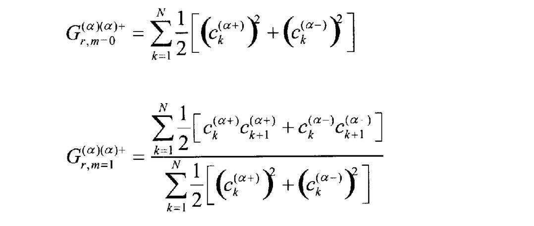
1)同一象限内の組み合せ
2)異なる象限の組み合せ
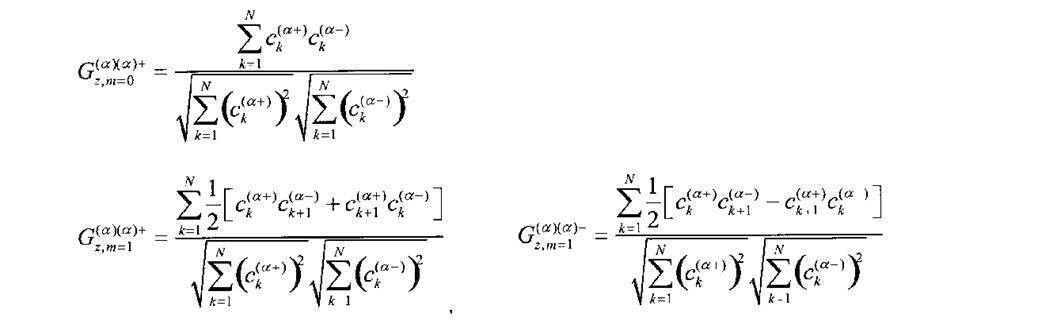
異なる色面間の基底関数の合成系による評価
1)同一象限内の組み合せ
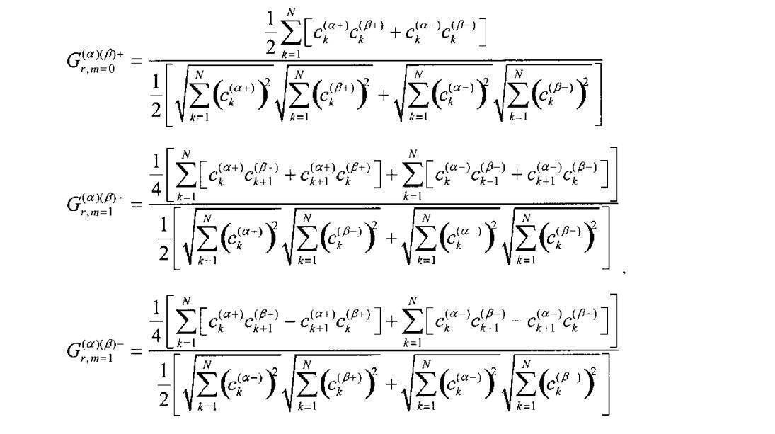
1)同一象限内の組み合せ
2)異なる象限の組み合せ
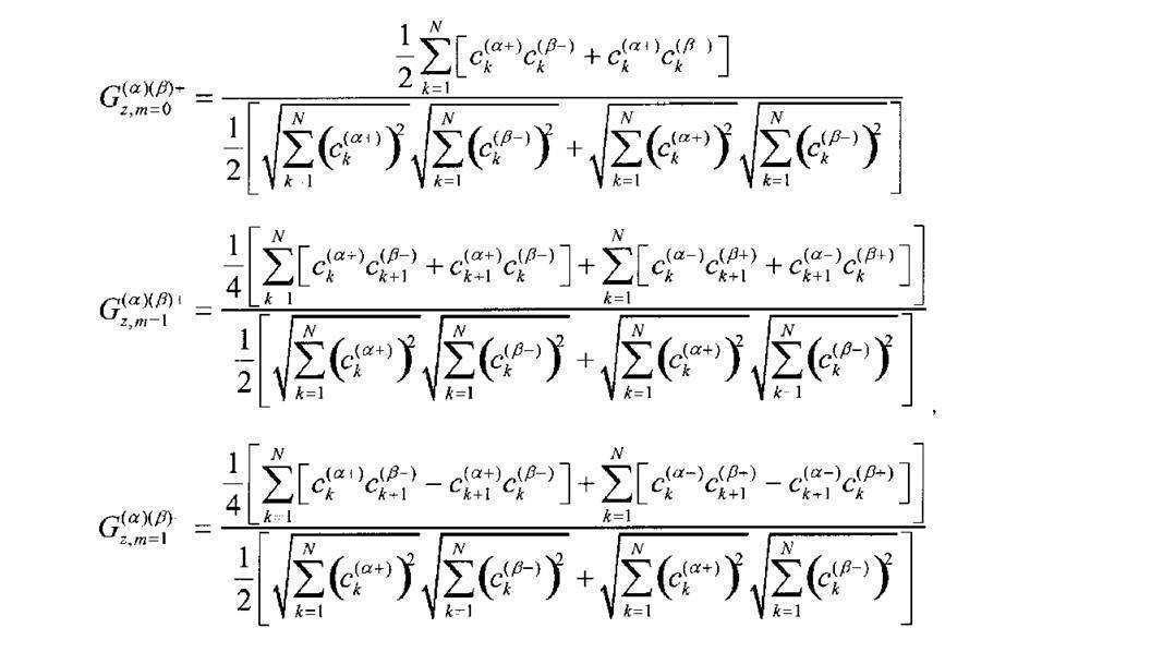
不変量のとりうる値とその性質は、第1の実施形態で説明した内容と全く同じであるので、ここでは省略する。
6.形容詞判別指標の作成
6-1.感性不変量の線形結合
ある感性形容詞(i)を検索するための指標として、感性不変量の加法性の性質を利用して、各々の感性不変量を線形結合した新たな指標Qiを作成する。指標Qiが表しうる形容詞は、1つの形容詞だけではなく、正反対の性質の形容詞を備えた一対の形容詞であるものとする。
Qi=β1G1+β2G2+...
ここに、Qiは再度[-1,1]の範囲の指標となるように、線型結合パラメータβiの値を規格化しておく。
6-1.感性不変量の線形結合
ある感性形容詞(i)を検索するための指標として、感性不変量の加法性の性質を利用して、各々の感性不変量を線形結合した新たな指標Qiを作成する。指標Qiが表しうる形容詞は、1つの形容詞だけではなく、正反対の性質の形容詞を備えた一対の形容詞であるものとする。
Qi=β1G1+β2G2+...
ここに、Qiは再度[-1,1]の範囲の指標となるように、線型結合パラメータβiの値を規格化しておく。
6-2.検索対象形容詞のパラメータ設定
所定の形容詞に対応する線形結合パラメータを事前に学習しておき、そのモデル・パラメータを設定する。
所定の形容詞に対応する線形結合パラメータを事前に学習しておき、そのモデル・パラメータを設定する。
7.画像分類処理
形容詞判別指標に基づいて、第1の実施形態と同様にして画像を分類する。以下に、実際にどのような感性を与える画像が抽出されるか具体例を挙げて示す。第1の実施形態と同様にテキスチャの場合も各々の感性不変量からは色彩心理学で用いられる高次の形容詞対と極めて深い関連性と線型性がある画像の整列を得ることができた。
形容詞判別指標に基づいて、第1の実施形態と同様にして画像を分類する。以下に、実際にどのような感性を与える画像が抽出されるか具体例を挙げて示す。第1の実施形態と同様にテキスチャの場合も各々の感性不変量からは色彩心理学で用いられる高次の形容詞対と極めて深い関連性と線型性がある画像の整列を得ることができた。
感性不変量の性質について全体を概観すると、異なる象限の基底関数を組み合わせることによって、分布関数の非対称性の要素が入った不変量の方が、感情的な要素が相当強く入ってくる。他方、同一象限内の基底関数を組み合わせた場合は、画像の被写体構造の多重性や一体性のような分離は可能であるものの、かなり中性的な側面も強い。以下に形容詞を割り当てながら例に挙げるのは主に異なる象限を組み合わせた場合を中心とする。
第1の実施形態の色の分布関数のときと少し事情が異なるのは、エッジの分布関数のときは非対角成分の要素が対角域から離れたところでも大きな値が残り、前者が対角域から離れると急速に強度が低下する短距離相関であるのに比べ、長距離相関の性質をもっているということである。これはテキスチャの分布構造によって誘起される感情の数のほうが色の分布構造によって誘起される感情の数よりも多いということを示していると解釈できる。
図11には

の相加平均をとった場合に、展開の次数がN=100で量子数差mをm=0,8,50とずらしたとき、整列させた画像群分布の両極端にはどのような分布関数の形状が該当するかを示した例である。上段は一方の端に位置する画像のV面のエッジ画像の分布関数の様子を、下段はもう一方の端に位置する画像の同様の様子を示している。
の相加平均をとった場合に、展開の次数がN=100で量子数差mをm=0,8,50とずらしたとき、整列させた画像群分布の両極端にはどのような分布関数の形状が該当するかを示した例である。上段は一方の端に位置する画像のV面のエッジ画像の分布関数の様子を、下段はもう一方の端に位置する画像の同様の様子を示している。
図11に対応する画像群の傾向として、m=0の上段には画像内で大柄な要素が存在して「豊かな」印象を与える画像が集まり、下段には「神妙な」印象を与える画像が集まる傾向が認められた。また、m=8からは上段には前後に2つの被写体が重なり、背景と主要被写体の2つの要素が存在するような複合的な画像が多く、下段には木々の葉や草が全面に映ったような細かなテキスチャ構造の一体的な画像が多く集まる。

この感性不変量からは「賑やかな-寂しい」と「華やかな-清楚な」という2つの形容詞対を合わせたような感性画像が整列する。「賑やかな、華やかな」画像には大柄な構造と小柄な構造が多数含まれるような様々なシーンの画像が集まる。一方の「寂しい、清楚な」画像には黒っぽい色の構造や暗い陰のシーンがある程度視覚的な影響力のある面積比重を伴って含まれている写真が多く集まる。

この感性不変量からは「しみじみとした-幽玄な」という形容詞対の感性画像が整列する。「しみじみとした」画像には木立と陰を伴った画像が多く集まる。一方の「幽玄な」画像には大面積の区分的な風景描写の上に、夕暮れ時のピンク色、オレンジ色、黄色などに染まった写真や、変わった雲の連なりの描写を伴っていたり、蒸気やもやが立ちこめたような画像が多く集まる。
図12に両端に選ばれた画像の典型例のエッジ画像と分布関数を示す。分布関数の形状から解説すると図12左側のようにV面とC面が共にエッジやテキスチャが多いとしみじみとした印象を与える。一方、図12右側のようにV面エッジ画像の分布関数がわずかな頻度で強い値を示す、すなわち分布関数に小さな裾野が存在していると元絵は山の稜線などで区分的に分断された画像構造を伴い、その上に輝度成分のコントラスト変化以上の太いコントラスト幅を伴って彩度面の変化が織りなすことによって幽玄な印象を与えると考えられる。

この感性不変量からは形容詞対を当てはめにくいが、「夏や昼の風景」と「秋・春や夕方の風景」という画像の対に明確に分離される。「夏や昼の風景」の画像は緑色や青色の面積が多く、コントラストが強い。「秋・春や夕方の風景」の画像は暖色系の色が含まれ、やや変化に乏しい画像が多い。
[第3の実施形態]
(テキスチャPDFのヒルベルト空間表現と感性不変量の線形和)
次に、第3の実施形態について説明する。第2の実施形態では統合エッジ画像のヒストグラムを右側と左側に分けて展開したが、左右同時展開するほうが対称性の議論もしやすく、望ましいので以下にその変更すべき点だけを記述する。そこから得られる感性不変量は、第2の実施形態よりも、感性との対応関係がとりやすく、より整列度の高いものとなると考えられる。
(テキスチャPDFのヒルベルト空間表現と感性不変量の線形和)
次に、第3の実施形態について説明する。第2の実施形態では統合エッジ画像のヒストグラムを右側と左側に分けて展開したが、左右同時展開するほうが対称性の議論もしやすく、望ましいので以下にその変更すべき点だけを記述する。そこから得られる感性不変量は、第2の実施形態よりも、感性との対応関係がとりやすく、より整列度の高いものとなると考えられる。
4.分布関数のヒルベルト空間表現
偶関数である0次の球ベッセル関数による根展開と、奇関数である1次の球ベッセル関数による根展開の二重級数によって、分布関数をヒルベルト空間表現する。そうすると分布関数形状の対称な成分は全て0次関数の展開係数に集まり、非対称な成分は全て1次関数の展開係数に集まることになる。なお、更に発展させて無限次数まで二重級数展開してもよい。
偶関数である0次の球ベッセル関数による根展開と、奇関数である1次の球ベッセル関数による根展開の二重級数によって、分布関数をヒルベルト空間表現する。そうすると分布関数形状の対称な成分は全て0次関数の展開係数に集まり、非対称な成分は全て1次関数の展開係数に集まることになる。なお、更に発展させて無限次数まで二重級数展開してもよい。
4-1.変数変換
ヒストグラムのピーク位置pから右側ないしは左側の最も遠くまで広がっている分布域の最端点までの距離をrとする。横軸の分布域は[-r+p, r+p]となる。この横軸を[-1,1]の区間に変数変換を行う。
横軸の変数変換:y=(x-p)/r
縦軸は第2の実施形態と同様。
ヒストグラムのピーク位置pから右側ないしは左側の最も遠くまで広がっている分布域の最端点までの距離をrとする。横軸の分布域は[-r+p, r+p]となる。この横軸を[-1,1]の区間に変数変換を行う。
横軸の変数変換:y=(x-p)/r
縦軸は第2の実施形態と同様。
4-2.球ベッセル関数の根と次数による二重級数展開
HVC各色面の分布関数をN個の0次と1次の球ベッセル関数の根による基底関数で展開する。ここで用いる記号aの意味は第2の実施形態と同様に、分布域の展開対象となる最外郭点を意味する。

HVC各色面の分布関数をN個の0次と1次の球ベッセル関数の根による基底関数で展開する。ここで用いる記号aの意味は第2の実施形態と同様に、分布域の展開対象となる最外郭点を意味する。
展開係数cnkは、基底関数の直交性を利用して、以下の式で求められる。

ここに、展開係数の算出式を導くにあたり、0次と1次関数の積は内部変数がいかにスケーリングされていても奇関数であることから、更にρ2の偶関数性を考慮して、左右対称区間で積分すると積分値がゼロになる性質を用いた。すなわち、次数に関する直交性の関係式は、偶数次と奇数次の関数の間で定義する限りにおいては重み関数が1の場合に留まらず、任意の偶関数の重みを加えても成り立つ。ただし、正規化の定数因子は変わるが、ρ2の場合は既に根による関係式で与えられている(概論説明の部分で記載)。
5.感性不変量の生成
二重展開係数cnkを1つのベクトルとして一重展開係数と同じように扱えば、第1の実施形態の色の感性不変量Fiと全く同様の形式の感性不変量Giを構築することができる。したがって、FをGに置き換えるだけでよい。ただし、和のとる範囲が2倍になり、k=1,2,...,N,N+1,...,2Nと変更することになる。このようにして求めた感性不変量を用いて第1及び第2の実施形態と同様に画像の分類を行うことができる。
二重展開係数cnkを1つのベクトルとして一重展開係数と同じように扱えば、第1の実施形態の色の感性不変量Fiと全く同様の形式の感性不変量Giを構築することができる。したがって、FをGに置き換えるだけでよい。ただし、和のとる範囲が2倍になり、k=1,2,...,N,N+1,...,2Nと変更することになる。このようにして求めた感性不変量を用いて第1及び第2の実施形態と同様に画像の分類を行うことができる。
[第4の実施形態]
(色とテキスチャの感性不変量の線形和)
次に、第4の実施形態について説明する。第1の実施形態で示した、画像の色信号分布に関する一次元分布関数から導いた感性不変量Fiと、第2、第3の実施形態で示した、エッジ画像の色信号分布に関する一次元分布関数から導いた感性不変量Giは、全く同じ次元の物理量であり相加的な性質を持っていることから、線形結合をすることにより両者は共通に扱うことができる。これは一次元分布関数に留まらず、構図の要素が絡んだ画像の色信号分布自体の2次元分布関数や更に高次の感性要素についても、同じ要領で感性不変量を構築すれば全く共通の土台に乗り、形容詞の階層構造で上位概念が最も強く残るという性質を感性の線型モデルによって説明することができるようになる。
<検索対象画像への処理>
1.マンセルHVC色空間への変換
この第4の実施形態においては、色相面はNの分離を行った面と行わない面の2つを用意する。その後の処理は第1~3の実施形態と同様である。
1.マンセルHVC色空間への変換
この第4の実施形態においては、色相面はNの分離を行った面と行わない面の2つを用意する。その後の処理は第1~3の実施形態と同様である。
5.形容詞判別指標の作成
Qi=α1G1+α2G2+...
+β1G1+β2G2+...
<感性形容詞モデル学習>
第1の実施形態とまったく同様の手法によって線型結合パラメータを決定する。
Qi=α1G1+α2G2+...
+β1G1+β2G2+...
<感性形容詞モデル学習>
第1の実施形態とまったく同様の手法によって線型結合パラメータを決定する。
ここでもう一度、これまでの説明を総括するとともに、更に新たな概念を導くための全体の概論説明を行う。その後にそれらを実現する第5~第7の実施形態について説明する。
[1]感性の定式化の描像
<基本概念>
感性の定式化の描像として次のように考える。1つ1つの画像がある感性に共通のエネルギー要素を発する。それを脳が知覚する。
[1]感性の定式化の描像
<基本概念>
感性の定式化の描像として次のように考える。1つ1つの画像がある感性に共通のエネルギー要素を発する。それを脳が知覚する。
<分布関数の形状特性>
図13は、色とテキスチャの分布関数を示す図である。これまで説明してきたように、画像の感性と分布関数の形状とは非常に関連性が深く、曖昧に似た形状が同一の感性を与える傾向にある。この分布関数の形状認識の定量化するために物理学的手法を導入してきた。
図13は、色とテキスチャの分布関数を示す図である。これまで説明してきたように、画像の感性と分布関数の形状とは非常に関連性が深く、曖昧に似た形状が同一の感性を与える傾向にある。この分布関数の形状認識の定量化するために物理学的手法を導入してきた。
<量子力学的手法>
これまでに説明してきた内容は、量子力学によって記述を試みるというものである。すなわち、次のように要約することができる。
1)分布関数fをヒルベルト空間に投影して運動量pを表示する。
2)群論を用いて2次形式の相加的なエネルギーEnを構築する。
ここでとった方法は実際には量子力学の概念を導入するとともに、画像という多数の画素と多数の階調を持った多体系のとる状態を、分布関数fを通して統計力学的に記述するという内容も含んでいる。それについて次に詳述する。
これまでに説明してきた内容は、量子力学によって記述を試みるというものである。すなわち、次のように要約することができる。
1)分布関数fをヒルベルト空間に投影して運動量pを表示する。
2)群論を用いて2次形式の相加的なエネルギーEnを構築する。
ここでとった方法は実際には量子力学の概念を導入するとともに、画像という多数の画素と多数の階調を持った多体系のとる状態を、分布関数fを通して統計力学的に記述するという内容も含んでいる。それについて次に詳述する。
<統計物理学的な意味>
上述の記述法の意味は、画像の信号値S(x,y)というミクロな性質の物理量から、感性という巨視的な性質の物理量への変換である。すなわち、ミクロな量の統計平均をとることによって、運動量と角運動量とエネルギーという力学的不変量のみが有効な成分として残り、その中でも画像群の統計平均をとることによって、エネルギーのみが有効な画像系を特徴づける役割を果たす。統計集団の作用によって、画像系はエネルギーバンドの構造とういう形に情報集約される。このように画像系のインフォメーションボリュームを縮約することによって、ミクロな性質からマクロな性質への変換を行う。統計力学的な記述法が、その統計的性質を記述するための橋渡しの役割を担う。
以下に、情報の縮約の様子を示す。構図系は未完であるが予測も含めて記述する。
画像信号S(x,y) 部分系情報f(p,q) エネルギー情報
~10^23個 色:(256)^3~10^7個 ~2000個
テキスチャ:(±256)^3~10^8個 ~2000個
構図:画素数~10^7個 (~2000個)
ここに、変数p,qは独立変数p1,p2,...,pi,...,q1,q2,...,qi,...から構成されているときでも、それらを代表する記号として用いる。
~10^23個 色:(256)^3~10^7個 ~2000個
テキスチャ:(±256)^3~10^8個 ~2000個
構図:画素数~10^7個 (~2000個)
ここに、変数p,qは独立変数p1,p2,...,pi,...,q1,q2,...,qi,...から構成されているときでも、それらを代表する記号として用いる。
<量子統計の密度行列による記述>
力学的記述をするに当たり、画像信号S(x,y)に対して何が位置座標q、運動量pに対応するかの考察が必要になる。その前に、画像系と量子統計との関わりについて説明する。
感性は、未知のハミルトニアン系で、かつ統計集団がなす力学系を取り扱う。統計力学で知られているように、巨視的な系全体を記述する波動関数は存在し得ない(文献E1参照)。画像系も巨視的な系を記述している。
力学的記述をするに当たり、画像信号S(x,y)に対して何が位置座標q、運動量pに対応するかの考察が必要になる。その前に、画像系と量子統計との関わりについて説明する。
感性は、未知のハミルトニアン系で、かつ統計集団がなす力学系を取り扱う。統計力学で知られているように、巨視的な系全体を記述する波動関数は存在し得ない(文献E1参照)。画像系も巨視的な系を記述している。
系に関する不完全なデータの組に基づく量子力学的記述は、密度行列を使って行われる。密度行列を使って任意の物理量の期待値が計算できるようになる。座標に関する密度行列は
ρ(q,q')=Σm,n wm,nψm*(q')ψn(q)
で表される。ある画像のある側面に関する部分系は、波動関数ψで完全に記述される状態にあるとすると、波動関数ψは完全系を作る関数ψn(q)で展開できる。
ψ=Σn cnψn
これを密度行列の表式に代入すると、エネルギー表示における密度行列
cm*cn→ wmn
を導くことができる。
ρ(q,q')=Σm,n wm,nψm*(q')ψn(q)
で表される。ある画像のある側面に関する部分系は、波動関数ψで完全に記述される状態にあるとすると、波動関数ψは完全系を作る関数ψn(q)で展開できる。
ψ=Σn cnψn
これを密度行列の表式に代入すると、エネルギー表示における密度行列
cm*cn→ wmn
を導くことができる。
エネルギー表示の密度行列の対角成分は定常状態を表す。一方の非対角成分は非定常状態を表す。画像はある瞬間のダイナミズムを捉えている。常に定常状態とは限らない。したがって、密度行列から導くエネルギー準位は非対角成分も考慮する必要がある。これは、非対角成分の記述は、密度行列を記述する波動関数の選び方に依存することを意味する。対角成分の定常状態ができるだけコンパクトに記述される波動関数系を選ぶのが、感性を記述する上で適切な選択である。統計物理学では、通常定常状態を考察の対象とするので、n番目の定常状態にある確率をwn=wnnと書く。
統計平均も定常状態による期待値を計算する。しかしながら、画像の感性は、定常状態にとどまらず、非定常状態も考察の対象とする必要がある。したがって、統計平均も定常状態と非定常状態の両方を考慮した期待値の計算が必要となる。
幾つもの画像群が同一の感性を与えるという、感性の曖昧性を扱うに当たり、感性の記述では全ての定常状態を対角和をとることによって定常状態を1つのエネルギー準位状態(E0)として扱い、また、非定常状態も同様に非対角成分同士の斜め和をとることによって、その定常状態から非定常状態へどれだけ離れた状態にあるかというエネルギー準位(En)によって記述する方法をとる。そのエネルギー準位への励起確率の統計分布をwn=w(En)で表す。物理的意味から、nの値が大きくなると画像系の中の運動の、より動的な状態、エネルギー遷移幅の大きい変化過程にある画像状態を記述しているといえる。この議論は、エネルギー行列を構築する過程においてもそのまま当てはめて定義を行う。
なお、エネルギーを定義してそれらの状態密度分布がρ(En)で表されたとすると、エネルギー準位への励起確率w(En)と合わせて、実際のエネルギーの確率分布はρ(En)w(En)で表される。
なお、エネルギーを定義してそれらの状態密度分布がρ(En)で表されたとすると、エネルギー準位への励起確率w(En)と合わせて、実際のエネルギーの確率分布はρ(En)w(En)で表される。
[文献E]ランダウ、リフシッツ理論物理学教程第5巻「統計物理学第1部」(第3版、1976年)、第1章「統計の基礎原理」、第2章「熱力学的諸量」、及び第3章「ギブス分布」
[文献E1]ランダウ、リフシッツ理論物理学教程第5巻「統計物理学第1部」(第3版、1976年)、第1章「統計の基礎原理」、第5節「統計行列」
[2]分布関数と感性の関連性について
<部分系と分布関数>
感性の記述にあたり、部分系に対する統計分布を見つけ出すことが重要な課題となる。感性における座標と運動量の力学変数q,pは、力学で定義されるような唯一のものとは限らない。感性の部分系として、画像のある側面を射影して、画像の性質を記述するに当たり、かなり独立性の高い側面を捉えた系と位置づける。
[文献E1]ランダウ、リフシッツ理論物理学教程第5巻「統計物理学第1部」(第3版、1976年)、第1章「統計の基礎原理」、第5節「統計行列」
[2]分布関数と感性の関連性について
<部分系と分布関数>
感性の記述にあたり、部分系に対する統計分布を見つけ出すことが重要な課題となる。感性における座標と運動量の力学変数q,pは、力学で定義されるような唯一のものとは限らない。感性の部分系として、画像のある側面を射影して、画像の性質を記述するに当たり、かなり独立性の高い側面を捉えた系と位置づける。
その側面の大分類として、色とテキスチャと構図の3主軸が考えられる。ただし、同じ画像を元に射影しているので、完全に独立ではないが、画像の情報を規定するに当たり、これらの3つの側面の分布関数が規定されると、統計的性質はほぼ記述するに足る情報を備えることになる。
ここでは、力学系の素朴な記述レベルにとどめ、更に高度な記述が必要となったときに、その完全独立でない記述法を考案する。これはある意味で、物理学の非相対論的な記述と相対論的な記述の関係に近い関係にある。すなわち、非相対論的記述では、位置座標系とスピン座標系は完全な独立系として記述されるが、相対論的記述ではその区別が不可能になり、位置座標とスピン座標が混合する座標系のスピノールによる記述に移行する必要があるという事情に相似しているためである。これらの部分系を各々記述した後に、統合することによって画像系の全体の感性を記述する。
<部分系の分布関数の記述と力学変数>
部分系毎に、力学変数である位置座標qと運動量pに対応する画像変数が異なって定義される。色は「零から正の有限値」の区間幅をもつ信号値の分布を表し、原信号そのものの分布を記述するから、その記述に適した線形微分方程式を満足する関数は、超幾何関数に含まれる何れかの関数である。テキスチャはエッジ成分を抽出した「負の有限値から正の有限値」の区間幅をもつ信号値の分布を表し、原信号の情報を1つ落とした別の側面の分布を記述するから、その記述に適した線形微分方程式を満足する関数は、合流型超幾何関数に含まれる何れかの関数である。構図は「零から正の有限値」の区間幅をもつ2次元的な信号値の分布を表し、原信号そのものの分布を記述するから、その記述に適した線形微分方程式を満足する関数は、超幾何関数に含まれる何れかの関数である。
部分系毎に、力学変数である位置座標qと運動量pに対応する画像変数が異なって定義される。色は「零から正の有限値」の区間幅をもつ信号値の分布を表し、原信号そのものの分布を記述するから、その記述に適した線形微分方程式を満足する関数は、超幾何関数に含まれる何れかの関数である。テキスチャはエッジ成分を抽出した「負の有限値から正の有限値」の区間幅をもつ信号値の分布を表し、原信号の情報を1つ落とした別の側面の分布を記述するから、その記述に適した線形微分方程式を満足する関数は、合流型超幾何関数に含まれる何れかの関数である。構図は「零から正の有限値」の区間幅をもつ2次元的な信号値の分布を表し、原信号そのものの分布を記述するから、その記述に適した線形微分方程式を満足する関数は、超幾何関数に含まれる何れかの関数である。
超幾何関数と合流型超幾何関数で記述される系は、側面の違う部分系を捉えていると考えることができる。すなわち、3つの特異点をもつ微分方程式で表される超幾何関数は、画像の信号値そのものの分布を表すのに適しており、分布関数の引数に来る画像信号として、画素値のように零以上の値で構成される画像信号が均質に分布しうる性質の記述に適している。一方、その内の2つの特異点を1つに合流させて合計2つの特異点をもつ微分方程式で表される合流型超幾何関数は、画像の信号値に関する情報量を1つ減らした側面を記述するのに適しており、分布関数の引数に来る画像信号として、微分操作によって1つの情報が落とされたエッジ信号値のように正と負の値にまたがる画像信号が零付近に局在化する性質の記述に適している。
<力学変数の変数分離の描像>
画像の部分系の側面を、物理学の物体粒子の記述における変数分離した座標系に対応させた描像を描いて記述する。色の一次元分布関数の記述に適した超幾何関数は、チェビシェフ関数であり、この関数は偶関数と奇関数の一重級数で完全系をなすため、偶関数を角運動量0、奇関数を角運動量1と捉えると、光と同じボーズ粒子であるスピン1のスピン座標を記述していると考えることができる。したがって、色の一次元分布関数は、波動関数のうちスピン系の波動関数を記述していると考えることができる。
画像の部分系の側面を、物理学の物体粒子の記述における変数分離した座標系に対応させた描像を描いて記述する。色の一次元分布関数の記述に適した超幾何関数は、チェビシェフ関数であり、この関数は偶関数と奇関数の一重級数で完全系をなすため、偶関数を角運動量0、奇関数を角運動量1と捉えると、光と同じボーズ粒子であるスピン1のスピン座標を記述していると考えることができる。したがって、色の一次元分布関数は、波動関数のうちスピン系の波動関数を記述していると考えることができる。
テキスチャの一次元分布関数の記述に適した合流型超幾何関数は、球ベッセル関数である。通常正の領域で定義される動径方向の波動関数の中でも、球ベッセル関数はベッセル関数のうち唯一負の領域に拡張定義できる関数である。したがって、テキスチャの一次元分布関数は、波動関数のうち動径方向の波動関数を記述していると捉えることができる。動径方向の波動関数は、偶関数と奇関数の次数と根に関する2つの級数の二重級数で記述することができるから、小さい方から角運動量0、1、2、3、...と割り当てることができ、それらは原子軌道ではs、p、d、f、...軌道と呼ばれているものに対応づけることができる。
構図の2次元分布関数の記述に適した超幾何関数は、ルジャンドル陪関数、ないしはそれとのフーリエ関数との合成積である球面調和関数が該当すると考えられる。したがって、構図の2次元分布関数は、球面座標表示における天頂角と方位角の2次元系座標に対応した波動関数を記述していると考えることができる。
<観測データの組と分布関数>
画像情報のある側面は、分布関数f(p,q)によって記述される。画像情報として観測されるデータと分布関数との間の関係を、次のように位置づける。すなわち、色:ヒストグラムをとって画素位置に関する情報を消失した分布関数、テキスチャ:エッジの側面のヒストグラムをとって画素位置に関する情報を消失した分布関数、構図:領域平均をとって画素数、すなわち画素位置に関する情報を減らした分布関数のように位置づける。この3つの分布関数を併せると、ほぼ画像S(x,y)というものの統計的性質を正確に反映する。印象の異なる別の画像が同値表現される確率は低い。ここに、画素位置と述べたものは力学変数p,qの位置座標qに対応するものとは一概には言えない。その対応関係を色とテキスチャについて、それぞれ2つずつの空間が定義できることを以下に述べる。
画像情報のある側面は、分布関数f(p,q)によって記述される。画像情報として観測されるデータと分布関数との間の関係を、次のように位置づける。すなわち、色:ヒストグラムをとって画素位置に関する情報を消失した分布関数、テキスチャ:エッジの側面のヒストグラムをとって画素位置に関する情報を消失した分布関数、構図:領域平均をとって画素数、すなわち画素位置に関する情報を減らした分布関数のように位置づける。この3つの分布関数を併せると、ほぼ画像S(x,y)というものの統計的性質を正確に反映する。印象の異なる別の画像が同値表現される確率は低い。ここに、画素位置と述べたものは力学変数p,qの位置座標qに対応するものとは一概には言えない。その対応関係を色とテキスチャについて、それぞれ2つずつの空間が定義できることを以下に述べる。
<座標空間と運動量空間>
(A)低次空間の側面
(A-1)色
マンセル色空間は色の強度分布を表す運動量空間とみなすことができる。
色ヒストグラム = f1(p)
(A-2)テキスチャ
多重解像度エッジ統合したエッジ画像のHVC各色面の色空間は、エッジの強度分布を表す運動量空間とみなすことができる。
テキスチャPDF = f3(p)
(B)高次空間の側面
(B-1)色
色ヒストグラムをチェビシェフ変換した場合、元の色ヒストグラム側を位置座標q、チェビシェフ展開係数側を運動量pとみなすことができる。高次運動量空間に投影した分布関数としては確率密度を表す必要があり、負の値をとらないので、展開係数側は係数を自乗したパワースペクトルをとる。
色ヒストグラム = f2(q) = f1(p)
チェビシェフ・スペクトル = f2(p)
(B-2)テキスチャ
テキスチャPDFを球ベッセル変換した場合、元のPDF側を位置座標q、球ベッセル展開係数側を運動量pとみなすことができる。同じく高次運動量空間の分布関数としては、パワースペクトルをとる。
テキスチャPDF = f4(q) = f3(p)
球ベッセル・スペクトル = f4(p)
図14は、これらの間の関係を分かりやすくするための概念図である。後に定義する各部分系のエントロピーの計算には、これらの分布関数を用いる。なお、エネルギー構築で2次形式を作る際に、通常のデカルト座標(x,y,z)における運動エネルギーの記述((px^2+py^2+pz^2)/(2m))とは違って、それに対応する色面内の相関の他に、色面間でも相関の要素を作って評価することに意味があるのは、マンセルHVCが完全に独立な成分ではないという事情が働いている。ただし、マンセルHVC色空間は心理量に対して等歩度になる均等色空間に設計されているので、各々の2次項の間の係数は伴わずに済む。
<統計平均に関する2つの意味>
画像系の統計的性質を導くための統計平均には2つの意味がある。すなわち、色、テキスチャ、構図の膨大な情報量が統計平均によって巨視的な物理量に縮約される点が1つである。また、多数のモデル画像群が共通の感性をなす意味において、画像群平均をとることによって、確定値を得る点がもう1つである。
画像系の統計的性質を導くための統計平均には2つの意味がある。すなわち、色、テキスチャ、構図の膨大な情報量が統計平均によって巨視的な物理量に縮約される点が1つである。また、多数のモデル画像群が共通の感性をなす意味において、画像群平均をとることによって、確定値を得る点がもう1つである。
前者は微視的な物理量から巨視的な物理量への変換過程に伴う、量子力学的な平均操作と統計的な平均操作を同時に含むものである。後者は巨視的な物理量のゆらぎの平均値に相当する量を決めて統計的性質を確定するための、統計的な平均操作を主に含むものと位置づけられる。したがって、前者は視覚系を通して脳に対して巨視的な働きかけを行う信号を作り、後者は人が受けた感覚の脳内の働きの分布の平均的要素を知る役割を担う。
[3]感性の記述とギブス分布
<画像群がなすエネルギーのゆらぎ>
多数画像群の共通感性の統計的性質を見いだす方法は、統計物理学のギブス分布(カノニカル分布)に対応する。すなわち、エネルギーのゆらぎを考慮した系の記述法である。一方、一枚画像の統計的性質を記述する方法は、ミクロカノニカル分布に対応する。これは、エネルギーのゆらぎを無視した系の記述法である。
<画像群がなすエネルギーのゆらぎ>
多数画像群の共通感性の統計的性質を見いだす方法は、統計物理学のギブス分布(カノニカル分布)に対応する。すなわち、エネルギーのゆらぎを考慮した系の記述法である。一方、一枚画像の統計的性質を記述する方法は、ミクロカノニカル分布に対応する。これは、エネルギーのゆらぎを無視した系の記述法である。
閉じた系(一枚画像)の運動量と角運動量はその系全体としての一様な並進運動と一様な回転運動に関係する。系の統計的性質を記述することにはならない。しかし、他の画像がもつ一様な並進運動と回転運動と区別する意味では意味を持つ。すなわち、一枚画像の閉じた系の並進運動と回転運動が静止する座標系をとれば、一枚画像の統計的性質を決定するのはエネルギーのみになるが、他の画像と共通の座標系で記述するとき、それらの画像群とは運動量と角運動量も異なっているので、それらが異なる画像と認識される。ただし、多数画像に共通の巨視的性質、すなわち、感性を記述するときには、運動量と角運動量は画像群の統計平均をとる量が増えると平均零あるいは定数値へと消滅する情報である。
<感性の曖昧性の記述と位相空間>
図15は、位相空間における感性群を示す描像図である。感性の記述は曖昧性を如何に定量的に記述するかという問題でもある。その統計物理学的な記述法の描像として、分布関数が一定の条件を満たす位相空間の軌跡が、同じ感性を呼び起こす状態分布を記述すると考える。一定の条件とは、力学的不変量であるエネルギーが一定値に拘束された条件を満たす位相空間上の軌道を表す。感性の曖昧性は、画像としては分布関数は様々な状態をとりうるが、それらが何れも同じ位相空間上のぼやけた範囲の軌跡上にある集合体として記述する。すなわち、分布関数から導かれる1つ1つのエネルギー要素が同じでなくても、それらの総和が同じ条件を満たしていれば、同じ感性を呼び起こすと考える。また、エネルギーのゆらぎをもつので、位相空間上では一定の幅をもったトラジェクトリーが同一の感性群に該当すると考える。その様子が図15では太線で広がるようにして描かれている。
図15は、位相空間における感性群を示す描像図である。感性の記述は曖昧性を如何に定量的に記述するかという問題でもある。その統計物理学的な記述法の描像として、分布関数が一定の条件を満たす位相空間の軌跡が、同じ感性を呼び起こす状態分布を記述すると考える。一定の条件とは、力学的不変量であるエネルギーが一定値に拘束された条件を満たす位相空間上の軌道を表す。感性の曖昧性は、画像としては分布関数は様々な状態をとりうるが、それらが何れも同じ位相空間上のぼやけた範囲の軌跡上にある集合体として記述する。すなわち、分布関数から導かれる1つ1つのエネルギー要素が同じでなくても、それらの総和が同じ条件を満たしていれば、同じ感性を呼び起こすと考える。また、エネルギーのゆらぎをもつので、位相空間上では一定の幅をもったトラジェクトリーが同一の感性群に該当すると考える。その様子が図15では太線で広がるようにして描かれている。
一般に分布関数の対数は、力学的不変量である運動の積分であり、相加的な運動の積分で記述される。すなわち、ある部分系の分布関数と別の部分系の分布関数が同時にその状態をとる確率を表す合成系の分布関数は部分系の分布関数の積で表され、その対数は相加的な性質を持つからである。そのような相加的な運動の積分は、力学で知られているように、エネルギーと運動量と角運動量のみが対応する。従って、分布関数の対数は、定数項αとそれらの各々にかかる定係数β、γ、δの一次結合によって記述されうる(文献E2=文献A3参照)。
[文献E2]ランダウ、リフシッツ理論物理学教程第5巻「統計物理学第1部」(第3版、1976年)、第1章「統計の基礎原理」、第4節「エネルギーの役割」
<少数モデルの位相空間軌道>
同一の感性を呼び起こす画像群の母集団画像が統計的に十分多い場合は、拘束条件はエネルギーのみとなる。これは、統計的性質の記述にはエネルギーだけが唯一相加的な運動の積分として残ることに由来する(文献E2=文献A3参照)。
<少数モデルの位相空間軌道>
同一の感性を呼び起こす画像群の母集団画像が統計的に十分多い場合は、拘束条件はエネルギーのみとなる。これは、統計的性質の記述にはエネルギーだけが唯一相加的な運動の積分として残ることに由来する(文献E2=文献A3参照)。
しかしながら、それらが少数の場合は、対応する感性の印象としては、それらの少数のモデルの細かな分布状態にも合致するような更に強い拘束条件が必要となる。そのための付加的拘束条件として役割を果たすのが、他の力学的不変量である運動量と角運動量であり、エネルギーに加えて運動量と角運動量もそれぞれが一定を満たす位相空間上の軌跡が、それら少数モデル画像に共通する感性作用を及ぼす分布範囲となる。少数モデルの極限として、一枚画像の類似画像検索が該当することになる。
<運動量表示と不確定性原理>
図16は、画像系の色とテキスチャに関する高次空間への投影で、位置と運動量の間の関係が不確定性原理を満たしている状況を説明する図である。すなわち、図16に例示したテキスチャPDFの場合のように、位置に関して鋭いピークが立って位置座標の確定精度が高いと、その波形を球ベッセル・フーリエ変換した運動量空間で実現しようとすると、あらゆる周波数を広く多く重ね合わせなければ達成できないため、運動量は不確定になり非常に広がった分布となる。一方、図16に例示した色ヒストグラムの場合のように、運動量空間であるチェビシェフ・フーリエ・スペクトルが極めて集中して表現されている場合、それを実空間表現すると、ある周波数の波が、この場合は低周波の波が全空間に渡って広がっている分布を表すことになる。したがって、位置が不確定となり、その広がり幅は大きい。すなわち、画像系においても周波数解析を行おうとすると、実空間において十分な区間幅の波形を見ない限り、そこに含まれる周波数成分は特定し得なくなる事実を記述した関係であると言い換えることができる。
図16は、画像系の色とテキスチャに関する高次空間への投影で、位置と運動量の間の関係が不確定性原理を満たしている状況を説明する図である。すなわち、図16に例示したテキスチャPDFの場合のように、位置に関して鋭いピークが立って位置座標の確定精度が高いと、その波形を球ベッセル・フーリエ変換した運動量空間で実現しようとすると、あらゆる周波数を広く多く重ね合わせなければ達成できないため、運動量は不確定になり非常に広がった分布となる。一方、図16に例示した色ヒストグラムの場合のように、運動量空間であるチェビシェフ・フーリエ・スペクトルが極めて集中して表現されている場合、それを実空間表現すると、ある周波数の波が、この場合は低周波の波が全空間に渡って広がっている分布を表すことになる。したがって、位置が不確定となり、その広がり幅は大きい。すなわち、画像系においても周波数解析を行おうとすると、実空間において十分な区間幅の波形を見ない限り、そこに含まれる周波数成分は特定し得なくなる事実を記述した関係であると言い換えることができる。
このような位置と運動量との間の拡張されたフーリエ変換の概念を通して、位置における波束と運動量における波束がそれぞれ一定幅以上に同時に実現することができないという不確定性関係は、量子力学において論じられている不確定性の原理に他ならない。量子力学におけるこの原理の説明は、例えば文献F1においてなされている。
プランク定数hの値は、画像系では、階調方向の量子化に関しては階調幅を規定するヒストグラムのビンが、空間方向の量子化に関しては画素間隔を規定する1画素という概念が関係している。したがって、画像系の階調数を減らしたり、縮小画像を生成したりするとプランク定数の値はその系の量子化の仕方に合わせて変更する必要があり、考察対象の状況によって変わる。この点は、物理定数のように部分系に関わらず、全系で一定として扱える状況とは異なる。しかし、画像系におけるプランク定数は、ある側面を投影した、量子化幅の規定された部分系においては固定値として扱える。
[文献F1] Landau and Lifshitz, Course of Theoretical Physics, Volume 3 "Quantum Mechanics (Non-Relativistic Theory)," (Third revised edition, 1977), Chapter 2 "Energy and Momentum," Section 16 "Uncertainty relations."
<位相空間と量子統計>
統計物理学の基礎的概念である位相空間上の軌跡は、量子力学的対応として状態数の概念を導入することが可能となり、画像から観測される物理量の状態数、あるいはそれらを規格化して密度表現した状態密度によって、画像感性の定量化が可能となる。
<位相空間と量子統計>
統計物理学の基礎的概念である位相空間上の軌跡は、量子力学的対応として状態数の概念を導入することが可能となり、画像から観測される物理量の状態数、あるいはそれらを規格化して密度表現した状態密度によって、画像感性の定量化が可能となる。
量子論的に位相空間上で、プランク定数で運動量と座標の両者の不確定量の数を割った量子状態数が定義できるようになると、巨視的な性質としてその対数で表される相加的な物理量であるエントロピーという概念が必然的に統計的に現れる。このエントロピーの概念を通して、巨視的体系のエネルギースペクトルの準位密度を決定することが、統計物理学的に理論的基礎づけされており、粒子数(ここでは画像系では画素数や階調数が対応)の増大に伴って準位間隔が指数関数的に減少し、連続的なエネルギーバンド構造になることが説明できる(文献E3参照)。
実際に実験によって連続的なエネルギー準位Enを算出した結果は、隣り合うエネルギー準位との間ではほとんど似通った性質を示すエネルギー要素に関する画像整列が見られるが、その中でもある性質の画像についてはエネルギー要素の分布内で遠距離に及ぶ順序の入れ替えが始まっており、エネルギー準位を端から端まで順にこの性質の様子を見て行くと、高エネルギー準位では低エネルギー準位とは全く異なる性質の画像整列が得られる。これはエネルギー準位密度が高密度化して、準位間の状態の区別がつかないエネルギーバンド構造の性質そのものを表している。なお、エントロピーとプランク定数との関係で結ばれるボルツマン定数に関しても、ある側面を投影した部分系においては固定値として扱えるが、異なる部分系の間では一般に定義は異なってくる。
[文献E3]ランダウ、リフシッツ理論物理学教程第5巻「統計物理学第1部」(第3版、1976年)、第1章「統計の基礎原理」、第7節「エントロピー」
<統計集団とエネルギー準位のバンド構造>
巨視的物体(ここでは画像)のエネルギー固有値のスペクトルにおける準位分布の異常な緻密さに帰着する(文献E1参照)。よって、画像系はエネルギーバンドの構造という形に情報集約される。
<統計集団とエネルギー準位のバンド構造>
巨視的物体(ここでは画像)のエネルギー固有値のスペクトルにおける準位分布の異常な緻密さに帰着する(文献E1参照)。よって、画像系はエネルギーバンドの構造という形に情報集約される。
ここで、物性と感性の理論構造の類似性について説明する。
純鉄と鉄の合金との性質の違いは、電子のエネルギーバンド構造の違いとして表現される(文献G1、G2、G3参照)。あるいは、強磁性体の鉄、ニッケル、コバルトの性質の違いがどのようにして生まれるのかは、電子構造を解明することによって記述することができる。また更に常磁性金属と強磁性金属の違い、あるいは常磁性金属のアルミニウムや銅などの性質の違いについても同様である。そして、物質の種類は、単体としては118種類の元素、それらの化合物、及び合金などからなり、数としては数千から一万個のオーダーで存在する。例えば、118個の元素の中から2~3個の元素の組み合わせ方の数を計算するとこのオーダーの数字になる。元素の数とその性質の根底を規定しているのが、原子軌道として存在しうる動径方向の波動関数s,p,d,f軌道とそれらの状態の縮退数である。
純鉄と鉄の合金との性質の違いは、電子のエネルギーバンド構造の違いとして表現される(文献G1、G2、G3参照)。あるいは、強磁性体の鉄、ニッケル、コバルトの性質の違いがどのようにして生まれるのかは、電子構造を解明することによって記述することができる。また更に常磁性金属と強磁性金属の違い、あるいは常磁性金属のアルミニウムや銅などの性質の違いについても同様である。そして、物質の種類は、単体としては118種類の元素、それらの化合物、及び合金などからなり、数としては数千から一万個のオーダーで存在する。例えば、118個の元素の中から2~3個の元素の組み合わせ方の数を計算するとこのオーダーの数字になる。元素の数とその性質の根底を規定しているのが、原子軌道として存在しうる動径方向の波動関数s,p,d,f軌道とそれらの状態の縮退数である。
同様に、感性形容詞も日本語の色感情を表す言葉として473語が代表的に存在し、それらの言葉で区別し得ないが、わずかに違うと心の中で感じる区別は、同様に数千から一万のオーダーで存在すると考えられる。この代表的473語の言葉の意味は、常にそれぞれが明確に違っているというものではなく、微妙な違いを表す表現も多く存在している。例えば、「賑やかな」に対しては「賑々しい」や「華やかな」、「華々しい」といった違う表現が存在する。一方、「爽やかな」と「賑やかな」という大分類の観点でかなり違う形容詞群も存在している。このように形容詞には大分類と微細分類の2面性が存在している。
このような2面性の性質は、物質の性質にも存在し、例えば元素の周期表でみれば、縦軸方向には上の方が、動径方向の波動関数がs軌道、p軌道と順に詰まった軽い電子系で、中間地帯はd軌道が詰まった遷移金属系、下の方はf軌道が詰まった重い電子系で、横軸方向にはそれらの軌道の電子の縮退数が1つずつ違うものが並ぶ。物質的な性質としては、縦方向に同列に存在する元素は化学的に極めて似た性質を示し、横方向に隣接して存在する場合も近い性質を示す。これらは、物質が固体としてアボガドロ数(~10^23)に及ぶ大集団として凝集するとき、統計的にエネルギーバンド構造をとり、それらの状態密度分布の違いとして、大きな性質の違いも小さな性質の違いも表現しうる。
したがって、感性もこのようなエネルギーバンドモデルで記述されることが最適な表現方法となる。なお、形容詞の2面性を位相空間上で表現すると、大分類で異なっている感性は、大きく軌跡が異なっているもの同士の状態分布の違い、微細分類でのみ異なっている感性は軌跡がかなり近いもの同士の状態分布の違いを表現しているものと考えられる。
したがって、感性もこのようなエネルギーバンドモデルで記述されることが最適な表現方法となる。なお、形容詞の2面性を位相空間上で表現すると、大分類で異なっている感性は、大きく軌跡が異なっているもの同士の状態分布の違い、微細分類でのみ異なっている感性は軌跡がかなり近いもの同士の状態分布の違いを表現しているものと考えられる。
[文献G1]Masako Akai, Hisazumi Akai and Junjiro Kanamori, "Electronic Structure of Impurities in Ferromagnetic Iron. I.s, p Valence Impurities," Journal of Physical Society of Japan, Vol.54, No.11, November, 1985, pp.4246-4256.
[文献G2]Masako Akai, Hisazumi Akai and Junjiro Kanamori, "Electronic Structure of Impurities in Ferromagnetic Iron. II. 3d and 4d Impurities," Journal of Physical Society of Japan, Vol.54, No.11, November, 1985, pp.4257-4264.
[文献G3]Masako Akai, Hisazumi Akai and Junjiro Kanamori, "Electronic Structure of Impurities in Ferromagnetic Iron. III. Light Interstitials," Journal of Physical Society of Japan, Vol.56, No.3, November, 1987, pp.1064-1077.
[4]巨視的物理量の記述
<エネルギー準位の描像モデル>
部分系への射影によって定義されるそれぞれの部分空間における運動量と位置の定義に基づいて、エネルギーを定義することができる。また、他の力学的不変量である角運動量も定義できる。エネルギーの構築方法として、低次の部分空間への射影の場合と高次の部分空間への射影の場合の2通りを各感性主軸について導入する。低次の部分空間への射影の場合は、エネルギーのモデルハミルトニアンを提案する方法をとる。一方の高次の部分空間への射影の場合は、エネルギー行列を構築し、定常状態から非定常状態に至るエネルギー固有値を定義する方法をとる。
低次の部分空間におけるエネルギー準位は、統計物理学の平均場近似によって作られる場のエネルギーを離散的なエネルギー準位と捉える。すなわち、離散的なスカラー不変量を構築する。高次の部分空間におけるエネルギー準位は、エネルギー行列の対角成分の定常状態から非対角成分の非定常状態へと徐々に離していく過程を、連続的なエネルギー準位と捉える。すなわち、連続的なベクトル不変量を構築する。
<色の低次不変量>
マンセルH,V,Cの値そのものが運動量を表していると考える。
モデル・ハミルトニアンを次のように構築する。
H=(H+V+C)^2
これは色の値の強度を表す運動エネルギーを表している。あるいは場のエネルギーを表している。
方程式
Hlψn>=Enlψn>
に対し、エネルギー固有値Enを求める。
エネルギー固有値の算出にあたり、統計物理学の平均場近似を用いる。
各運動量を平均項とゆらぎ項に分けて、ゆらぎ項も平均的なゆらぎ幅によって記述する。すなわち、ゆらぎ項として標準偏差をとり、平均値と同じ運動量pの次元を持つようにする。
√<(H-<H>)^2> ~= σH
√<(V-<V>)^2> ~= σV
√<(C-<C>)^2> ~= σC
これらの運動量の平均値と標準偏差値は、運動量分布を表す分布関数f(p)から求める。すなわち、H,V,Cの色ヒストグラムf(H),f(V),f(C)から求める。
H=(H+V+C)^2
={(<H>+(H-<H>)+(<V>+(V-<V>)+<C>+(C-<C>)}^2
~={(<H>+σH)+(<V>+σV)+(<C>+σC)}^2
=(<H><H>+<V><V>+<C><C>)
+2(<H><V>+<V><C>+<C><H>)
+2(<H>σH+<V>σV+<C>σC)
+2(<H>σV+<V>σC+<C>σH)
+2(σH<V>+σV<C>+σC<H>)
+(σHσH+σVσV+σCσC)
+2(σHσV+σVσC+σCσH)
このようにハミルトニアンを平均場とゆらぎ場に近似して2次形式として導出される要素が、1つ1つのエネルギー要素に対応し、離散的なエネルギー準位を作る。各画像によって、それらのエネルギー要素がとる値は異なってくるが、ある感性をもつ画像群の間では、あるエネルギー要素が共通に強く作用する因子として、作用していることが画像群の分布を調べることによって見えてくることになる。
一般に、画像の色ヒストグラムをとってみれば分かるように、運動量の分布は画像によって極めてランダムに変化する変動性の強い特性をもち、同一の感性をもつ画像群で統計平均をとっても、共通因子の要素はほとんど残らない。しかしながら、エネルギーの形である2次形式という状態で分布を観察すると、同一の感性を持つ画像群で共通に作用する因子が残留しやすくなる。例えば、「殺風景な」という画像は、平均輝度<V>と平均彩度<C>が同時に小さな値をとっている確率が高く、<V><C>という運動エネルギーは共通に小さな値を示していることが多い。ただし、ある場合は<V>の値が大きめに出ている場合もあり、そのときは<C>側がもっと小さな値を示すことによってバランスをとる。このようなとき<V>と<C>を個別に統計平均をとると、それらの運動量平均は、値として一般画像の平均値に情報として消滅してしまいやすい。この様子を以下に示す。
運動量p エネルギーEn
色相H 統計平均 <V><C>
輝度V ⇒ <V><V>
彩度C 残存情報 <H>σV
σCσC
...
(ランダム分布) (同時性の整列)
1)運動量
運動量の要素pnとしては以下のものが挙げられる。
<H>, <V>, <C>, σH, σV, σC
なお、σの部分は角運動量の要素Mnとして扱ってもよい。
運動量p エネルギーEn
色相H 統計平均 <V><C>
輝度V ⇒ <V><V>
彩度C 残存情報 <H>σV
σCσC
...
(ランダム分布) (同時性の整列)
1)運動量
運動量の要素pnとしては以下のものが挙げられる。
<H>, <V>, <C>, σH, σV, σC
なお、σの部分は角運動量の要素Mnとして扱ってもよい。
2)エネルギー
エネルギーの要素Enとしては以下のものが挙げられる。エネルギー要素Enについて、種類の異なるエネルギー要素が算出されるので、それらを区別するための記号として以下のような省略記号でそれらの状態を表すことにする。α面にはa、β面にはb、平均値にはm、標準偏差値にはsの記号を用いる。
(α)(α)
amam: <H><H>, <V><V>, <C><C>,
amas: <H>σH, <V>σV, <C>σC,
asas: σHσH, σVσV, σCσC,
(α)(β)
ambm: <H><V>, <V><C>, <C><H>,
ambs: <H>σV, <V>σC, <C>σH,
asbm: σH<V>, σV<C>, σC<H>,
asbs: σHσV, σVσC, σCσH
色の低次不変量に関しては、下記に記す注意点を考慮すると<H>を伴う項は、2つの要素に分離する。したがって、色の低次不変量のエネルギー要素としては、21+5=26種類のスカラー不変量が導出される。これらは各々、離散的なエネルギー準位Enに対応し、Enの値そのものを表す。これが、色の低次部分系で縮約されてきた巨視的な物理量である。
3)色の低次不変量の場合の特殊事項
色相Hはマンセル色空間変換時にニュートラルNとそれ以外の色相環H(≠N)によって表される。分布関数f(H)は、第1の実施形態で説明したように色相環のヒストグラム・ビンとNのヒストグラム・ビンに分かれたヒストグラムを用いる。また、色相環で平均値を算出するとき、第1の実施形態でチェビシェフ展開するときの色相環の起点を定義したのと同様に、色相環内で分布関数が最小となる点に切り込みを入れ、それより値の小さい領域は、色相環の角度の最大値側の端点に2π角度分の値を追加する形で値を大きく延ばして領域を確保し、その軸上で平均マンセル色相値を算出する。その値が元のマンセル色相値の値範囲を超えている場合は、2π角度分に相当する値を引いて元に戻す。
色相Hはマンセル色空間変換時にニュートラルNとそれ以外の色相環H(≠N)によって表される。分布関数f(H)は、第1の実施形態で説明したように色相環のヒストグラム・ビンとNのヒストグラム・ビンに分かれたヒストグラムを用いる。また、色相環で平均値を算出するとき、第1の実施形態でチェビシェフ展開するときの色相環の起点を定義したのと同様に、色相環内で分布関数が最小となる点に切り込みを入れ、それより値の小さい領域は、色相環の角度の最大値側の端点に2π角度分の値を追加する形で値を大きく延ばして領域を確保し、その軸上で平均マンセル色相値を算出する。その値が元のマンセル色相値の値範囲を超えている場合は、2π角度分に相当する値を引いて元に戻す。
色相環を表すために<H>は複素数表現して2成分に分離し、その記述を実現する。また、そのときに複素数の絶対値の大きさによって色相環に残っているニュートラル分を差し引いた割合を表す。
<H>=(1-pop(N))exp(2πi<H(≠N)>/100)
σHは色相環内の分布関数のみの広がり幅を計算する。したがって、1成分のままである。こちらの強度も<H>の絶対値の大きさと連動して、色相環に残っている度数割合を掛け算して評価する。すなわち、全てがニュートラルに流れ込んだ場合は、必ずσHが零になるように定義する。
σH=(1-pop(N)) σH(≠N)
<テキスチャの低次不変量>
テキスチャを表すエッジ面として、第2の実施形態で説明した、マンセルHVC面の各々を多重解像度変換し、高周波サブバンド画像だけを逆変換によって統合した統合エッジ面を利用する。そのエッジ面のエッジ強度は、模式的にラプラシアン記号△を用いて、△H,△V,△Cと表す。
今度はHVC面のエッジ強度△H,△V,△Cの値そのものが運動量を表していると考える。
モデル・ハミルトニアンを次のように構築する。
H=(△H+△V+△C)^2
これは色のエッジ成分の値の強度を表す運動エネルギー、あるいは場のエネルギーを表している。
エネルギー固有値Enを色の低次不変量のときと同様に平均場近似によって求める。運動量の平均値と標準偏差値は、運動量分布を表す分布関数f(p)から求める。すなわち、△H,△V,△Cのエッジ強度のヒストグラムf(△H),f(△V),f(△C)から求める。
色の低次不変量のときと同様の手続きによって、テキスチャの低次不変量が求まる。
1)運動量
運動量の要素pnとしては以下のものが挙げられる。
<△H>, <△V>, <△C>, σ△H, σ△V, σ△C
なお、σの部分は角運動量の要素Mnとして扱ってもよい。
色の低次不変量のときと同様の手続きによって、テキスチャの低次不変量が求まる。
1)運動量
運動量の要素pnとしては以下のものが挙げられる。
<△H>, <△V>, <△C>, σ△H, σ△V, σ△C
なお、σの部分は角運動量の要素Mnとして扱ってもよい。
2)エネルギー
エネルギーの要素Enとしては以下のものが挙げられる。エネルギー要素Enについて、種類の異なるエネルギー要素が算出されるので、それらを区別するための記号として以下のような省略記号でそれらの状態を表すことにする。α面にはa、β面にはb、平均値にはm、標準偏差値にはsの記号を用いる。
(α)(α)
amam: <△H><△H>, <△V><△V>, <△C><△C>,
amas: <△H>σ△H, <△V>σ△V, <△C>σ△C,
asas: σ△Hσ△H, σ△Vσ△V, σ△Cσ△C,
(α)(β)
ambm: <△H><△V>, <△V><△C>, <△C><△H>,
ambs: <△H>σ△V, <△V>σ△C, <△C>σ△H,
asbm: σ△H<△V>, σ△V<△C>, σ△C<△H>,
asbs: σ△Hσ△V, σ△Vσ△C, σ△Cσ△H,
テキスチャの低次不変量のエネルギー要素としては、21種類のスカラー不変量が導出される。これらは各々、離散的なエネルギー準位Enに対応し、Enの値そのものを表す。これが、テキスチャの低次部分系で縮約されてきた巨視的な物理量である。
3)テキスチャの低次不変量の場合の特殊事項
色相面のエッジ成分は、マンセル値が0の点を常に色相環の原点とした値で表示した色面のエッジをとるものとする。なぜならば、実験的に色相環の切り込み点を画像毎に分布関数が最小となる点に変化させるよりも、虹色のスペクトル分布と同じマンセル値の原点で固定的に観測した方が色相面のエッジとしては好ましいことが判明したからである。また、ニュートラルは別扱いせずに色相環の何れかの点に分布する色相面とする。よって、ニュートラル成分は色相面上のランダムノイズのように振る舞う。
色相面のエッジ成分は、マンセル値が0の点を常に色相環の原点とした値で表示した色面のエッジをとるものとする。なぜならば、実験的に色相環の切り込み点を画像毎に分布関数が最小となる点に変化させるよりも、虹色のスペクトル分布と同じマンセル値の原点で固定的に観測した方が色相面のエッジとしては好ましいことが判明したからである。また、ニュートラルは別扱いせずに色相環の何れかの点に分布する色相面とする。よって、ニュートラル成分は色相面上のランダムノイズのように振る舞う。
<色の高次不変量>
色の分布関数をチェビシェフ展開する。変数xは、H,V,Cの各々の値をとる。

分布関数から力学的不変量である運動量、角運動量、エネルギーを導くにあたり、分布関数の形状を記述するのに独立な形状評価をしうる成分を可能な限り導き出す。すなわち、エネルギーや角運動量を構築するに当たり、分布関数f(x)を軸反転したf(-x)も考察対象に加える。色の場合は、軸反転することの物理的意味は階調反転することに相当する。そのために角運動量の概念を導入する。すなわち、基底関数群を偶関数と奇関数の性質の違いによって部分群に分け、各々の部分群に角運動量量子数を割り当てる。
色の分布関数をチェビシェフ展開する。変数xは、H,V,Cの各々の値をとる。
分布関数から力学的不変量である運動量、角運動量、エネルギーを導くにあたり、分布関数の形状を記述するのに独立な形状評価をしうる成分を可能な限り導き出す。すなわち、エネルギーや角運動量を構築するに当たり、分布関数f(x)を軸反転したf(-x)も考察対象に加える。色の場合は、軸反転することの物理的意味は階調反転することに相当する。そのために角運動量の概念を導入する。すなわち、基底関数群を偶関数と奇関数の性質の違いによって部分群に分け、各々の部分群に角運動量量子数を割り当てる。
チェビシェフ基底は、偶数番目の基底が偶関数でψ(-x)=ψ(x)の関係を満たし、奇数番目の基底が奇関数でψ(-x)=-ψ(x)の関係を満たす。よって、偶関数群には角運動量量子数l=0、奇関数群には角運動量量子数l=1を割り当てる。軸反転x→-xすることによって、奇数番目の角運動量量子数の基底関数は符号反転し、偶数番目の角運動量子数の基底関数は符号は不変である。このような角運動量単位の波動関数の軸反転に関する性質を量子力学ではパリティと呼ぶ。偶関数の基底関数は偶のパリティを持ち、軸反転に対して不変であり、奇関数の基底関数は奇のパリティを持ち、軸反転に対して符号を反転する。
この角運動量量子数がスピン系を記述していると考えると、色はスピン角運動量量子数s=1の系を記述していることになる。チェビシェフ関数は、一重級数展開のみで定義され、偶関数と奇関数はそれぞれスピン0とスピン1の状態を記述し、軸反転によりスピン1の状態のパリティが反転した状態を生み出すことができる。チェビシェフ関数はボーズ粒子であるスピン1の系の記述に適している。
独立な成分を考察するにあたり、まず最初に系を記述する角運動量の軸反転しない場合の運動量の要素pn、角運動量の要素Mn、エネルギーの要素Enを構築した上で、それらの各々を角運動量の軸反転した約倍の要素を導く。そのとき、全要素を線形結合したときに線形結合係数が意味のある独立成分を記述する否かの観点で導く。すなわち、要素の符号が変わるだけのときは、線形結合係数の符号を変えれば同じ系を記述するため、意味をなさない。一般に運動量はこの部類に入るが、角運動量とエネルギーは別の独立な成分が導き出せる。
具体例を挙げるために、展開係数の数2Nを200とする。すなわちN=100とする。
具体例を挙げるために、展開係数の数2Nを200とする。すなわちN=100とする。
1)運動量
運動量の要素pnとしては以下のものが挙げられる。
cn (α) ここに、(α)=H,V,C。
2N=200のとき運動量の要素の数は3面分あるから、200x3=600個である。
運動量の要素pnとしては以下のものが挙げられる。
cn (α) ここに、(α)=H,V,C。
2N=200のとき運動量の要素の数は3面分あるから、200x3=600個である。
2)角運動量
以下では、cnを角運動量単位の部分群に分けて考える場合は、角運動量量子数l=0の展開係数をc0n、角運動量量子数l=1の展開係数をc1nと表すことにする。したがって、展開係数の要素数は半々のN個ずつに分かれる。部分群の要素番号はn=1,2,...,Nで数えるものとする。
角運動量の要素Mnとしては以下のものが挙げられる。
0*(c01 (α)+c02 (α)+...+c0N (α))+1*(c11 (α)+c12 (α)+...+c1N (α))
=(c11 (α)+c12 (α)+...+c1N (α)) ここに、(α)=H,V,C。
以下では、cnを角運動量単位の部分群に分けて考える場合は、角運動量量子数l=0の展開係数をc0n、角運動量量子数l=1の展開係数をc1nと表すことにする。したがって、展開係数の要素数は半々のN個ずつに分かれる。部分群の要素番号はn=1,2,...,Nで数えるものとする。
角運動量の要素Mnとしては以下のものが挙げられる。
0*(c01 (α)+c02 (α)+...+c0N (α))+1*(c11 (α)+c12 (α)+...+c1N (α))
=(c11 (α)+c12 (α)+...+c1N (α)) ここに、(α)=H,V,C。
角運動量がl=1までしか存在しない場合は、独立な成分は上記の1つだけとなる。なぜならば、角運動量の軸を反転した
0*(c01 (α)+c02 (α)+...+c0N (α))-1*(c11 (α)+c12 (α)+...+c1N (α))=-(c11 (α)+c12 (α)+...+c1N (α))は上と同じ系を記述しているにすぎないからである。
0*(c01 (α)+c02 (α)+...+c0N (α))-1*(c11 (α)+c12 (α)+...+c1N (α))=-(c11 (α)+c12 (α)+...+c1N (α))は上と同じ系を記述しているにすぎないからである。
このように奇関数の展開係数の一次和は、分布関数の非対称性を評価するための巨視的な指標となりうる。古典的な角運動量の定義はM=rxpであるが、それと対比すると上述の定義は運動量の部分和に対してヒルベルト空間座標の角運動量量子数を原点からの距離とする座標空間で積をとることで、分布関数のモーメントを記述していることになる。
角運動量の要素の数は3面分あるから1x3=3個である。
角運動量の要素の数は3面分あるから1x3=3個である。
3)エネルギー
α面とβ面の運動量の積をとって、運動エネルギーを構築する。運動量の積cm*cnは群論では直積あるいはクロネッカー積と呼ばれる行列を作るが、同じ基底関数で表された2つの系の積行列は可約な表現で、より小さな次元の2つの表現に分解することができる。
すなわち、対称積と反対称積の行列表現に分解することができ、
(α)面と(α)面の積からは対称積のエネルギー行列(i,k)が構築できる。
ci (α)ck (α)+ck (α)ci (α)
また、(α)面と(β)面の積からは対称積と反対称積のエネルギー行列(i,k)が構築できる。
ci (α)ck (β)+ck (α)ci (β)
ci (α)ck (β)-ck (α)ci (β)
なお、これらは何れも基底関数の数だけ縦と横に並んだ正方行列である。
エネルギーの固有値を算出するため、対角和、すなわちシュプールをとるものとする。定常状態のエネルギー固有値は純粋に対角和をとったものである。これがn=0すなわちi=kの場合のエネルギー要素Enである。非定常状態のエネルギー固有値を算出するため、n=i-kだけ対角成分から離れた行列要素の和をとる拡張シュプールを定義する。通常のシュプールとは異なるためSp’という記号を用いる。このときシュプールをとる要素の数は、必ず対角和の要素の数と同じになるように定義して、積の一方で用いられる基底関数群は、必ず完全系をなす基底関数を全て一度なめる形で構築する。これは対称積と反対称積に分解するときの規則として課される要件である。そのために、n=i-kを満たす行列要素群で和をとる操作をしたとき、行列の端ではみ出してしまう要素については、考察対象の行列あるいは部分行列の大きさをNとするとそれらの行列内でn+N=i-kとなるように対角成分を挟んで反対側の領域で残りの要素数だけ斜め和をとるように定義する。こうしてエネルギー要素Enが順次算出される。なお、具体例は第1の実施形態と第3の実施形態に記述済みである。
エネルギー要素の数は、1つのエネルギー行列に対して基底関数の展開係数の数の半分に相当する数だけ存在する。半分になる理由は行列からはみ出した成分を行列幅に等しい数だけずらしてもう一度織り込んでくるから、それらが順になめていった場合2重定義となるから、有効なのは半分に減ずるためである。すなわち、拡張シュプールをとることによって2次元の行列要素は各行と列をなす一次元の要素の数の半分に等しい数にまでエネルギー要素の数は縮約する。
次に角運動量の軸を反転した状態を考察する。上述の3つのエネルギー行列の定義は、(α)面と(α)面、及び(α)面と(β)面からなる表面と表面の積による表の姿の描写をしている。それに対して一方の分布関数を軸反転することによって裏面の(-α)面や(-β)面を作ることができる。行列積を作るときに一方を表面にとりもう一方を裏面にとることによって、裏の姿の描写をすることが可能になる。これによって、独立なエネルギー要素の導出が可能になる。すなわち、パリティの概念を導入することによって、独立な合成系の基底関数を構築する。なお、パリティは古典力学では出てこない概念である。
ここで、(α)面と(-α)面の積からは対称積と反対称積のエネルギー行列(i,k)が構築できる。
ci (α)ck (-α)+ck (α)ci (-α)
ci (α)ck (-α)-ck (α)ci (-α)
また、(α)面と(-β)面の積からは対称積と反対称積のエネルギー行列(i,k)が構築できる。
ci (α)ck (-β)+ck (α)ci (-β)
ci (α)ck (-β)-ck (α)ci (-β)
これらのエネルギー行列の要素の各々はck (-α)のうちのkが奇関数に相当している場合だけは、ck (-α)=-ck (α)と符号が反転し、偶関数に相当している場合はck (-α)=ck (α)のように符号を変えないようなエネルギー行列を構築する。このように一部の要素で符号反転した裏の姿の行列内で、表の姿の行列と同様な拡張シュプールをとっていくと、個別に出てくるエネルギー要素として独立な成分が導出できる。
これらの表の姿のエネルギー行列の拡張シュプールや、裏の姿のエネルギー行列の拡張シュプールをとるに当たり、角運動量による部分群が定義できるときの基底関数の並べ方には2通りが考えられる。すなわち、第1番目は角運動量量子数の低い順から先に並べる方法である。

第2番目は主量子数の低い順番から先に並べる方法である。

これらを順番にψiと一次元の指標を与え、2次元の行列積として対称積と反対称積ψiψk±ψkψiを作ると、第1番目の項と第2番目の項のiとkは対角成分を挟んで交換することになる。これらのエネルギー行列をもう一度、角運動量単位で部分行列に分けて並べると、部分行列内でn=i-kを満たす拡張シュプールをとることと等価になる。ただし、i,kを角運動量量子数と主量子数の2つのインデックスを用いて表した場合、第1番目の並べ方の場合は単純に同じ角運動量量子数の組み合せの部分行列内で主量子数のiとkを交換した形で表せるが、第2番目の並べ方を採用した場合、少しそれとは異なる表現となるので注意を要する。すなわち、同じ距離の非対角位置に存在する部分行列の要素との間でi,kを交換するとき、第1項目のψiψkのψi側がψk側よりも大きな角運動量量子数の場合は、n=i-k個だけ右側に来るψの主量子数はψi側の主量子数よりも1つだけ繰り上がったk+1として表記しなければならない。その後に、どちらの並べ替えをした場合であっても、要素を交換した2つの部分行列の間で、部分行列単位で要素をまとめる操作を行って部分行列表現する。
第2番目は主量子数の低い順番から先に並べる方法である。
これらを順番にψiと一次元の指標を与え、2次元の行列積として対称積と反対称積ψiψk±ψkψiを作ると、第1番目の項と第2番目の項のiとkは対角成分を挟んで交換することになる。これらのエネルギー行列をもう一度、角運動量単位で部分行列に分けて並べると、部分行列内でn=i-kを満たす拡張シュプールをとることと等価になる。ただし、i,kを角運動量量子数と主量子数の2つのインデックスを用いて表した場合、第1番目の並べ方の場合は単純に同じ角運動量量子数の組み合せの部分行列内で主量子数のiとkを交換した形で表せるが、第2番目の並べ方を採用した場合、少しそれとは異なる表現となるので注意を要する。すなわち、同じ距離の非対角位置に存在する部分行列の要素との間でi,kを交換するとき、第1項目のψiψkのψi側がψk側よりも大きな角運動量量子数の場合は、n=i-k個だけ右側に来るψの主量子数はψi側の主量子数よりも1つだけ繰り上がったk+1として表記しなければならない。その後に、どちらの並べ替えをした場合であっても、要素を交換した2つの部分行列の間で、部分行列単位で要素をまとめる操作を行って部分行列表現する。
実験的に(α)面と(α)面の積を作るときは第1番目の並べ方の方が優れ、(α)面と(β)面の積を作るときは第2番目の並べ方の方が優れるということが判明した。これは、第1番目の並べ方は異なる角運動量量子数の間は完全に独立系と扱えることを前提としており、同一面内では完全直交系の基底関数の展開によってそれが満たされていることを意味する。一方の第2番目の並べ方は異なる角運動量量子数との間であっても近接した主量子数の間の基底関数で記述した方がその密接に関与し合っている様子を記述できることを表しており、HVC面が完全な独立な系を記述していないことに起因すると考えられる。
このような部分行列を組み合わせる方法としては、拡張シュプールが完全系をなす全ての基底関数をなめるように部分行列の間で和をとる必要がある。すなわち、運動量の要素が、角運動量量子数が0と1の系からなる2つの部分群に分かれているときは、エネルギー行列は角運動量の固有状態を表す2つの部分行列と角運動量の混合状態を表す2つの部分行列に分けて考えることができる。このとき、完全系をなすようになめる拡張シュプールの取り方として、2つの対角部分行列のシュプールをつなげる場合と、2つの非対角部分行列のシュプールをつなげる場合と2通りが存在する。このように角運動量単位でエネルギー行列を分けて考えた方が物理的意味が明確になる。
この様子を模式的に表すと以下のようになる。
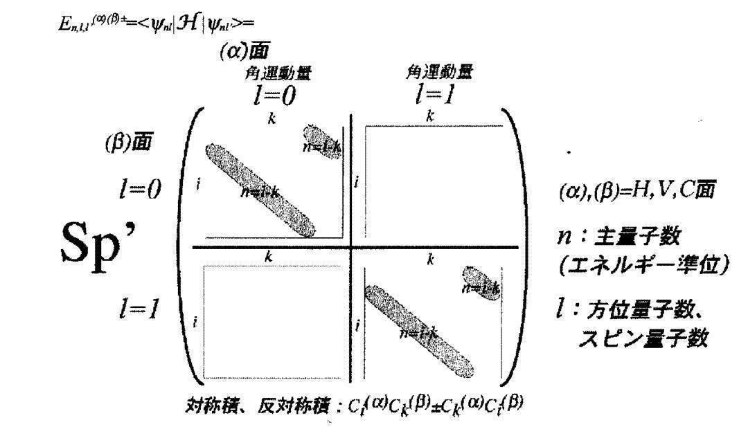
この様子を模式的に表すと以下のようになる。
同じサフィックスが出てきたときには、それらについて和をとるものとする。
実際にエネルギー行列を角運動量の部分行列に分けて拡張シュプールを組むための部分行列和の具体例を示す。以下には部分行列をなす2つの基底関数の合成系の形式で表現し、部分行列と部分行列の和も同時に示す。各部分行列はこれらの基底関数ψikをcikに置き換えるだけで得られる。したがって、各部分行列が(i,k)で定義されると、エネルギー要素Enを算出するには、それぞれの部分行列内でn=i-kを満たす行列要素についてシュプールをとる。
実際にエネルギー行列を角運動量の部分行列に分けて拡張シュプールを組むための部分行列和の具体例を示す。以下には部分行列をなす2つの基底関数の合成系の形式で表現し、部分行列と部分行列の和も同時に示す。各部分行列はこれらの基底関数ψikをcikに置き換えるだけで得られる。したがって、各部分行列が(i,k)で定義されると、エネルギー要素Enを算出するには、それぞれの部分行列内でn=i-kを満たす行列要素についてシュプールをとる。
エネルギー要素Enについてシュプールを実行する部分群単位で、種類の異なるエネルギー要素が算出されるので、それらを区別するための記号として以下のような省略記号でそれらの状態を表すことにする。α面にはa、β面にはb、角運動量が固有状態の(l,l')=(0,0)+(1,1)の組み合せに対しては00記号を、角運動量が混合状態の(l,l')=(0,1)+(1,0)の組み合せに対しては01記号を、対称行列にはプラスのp記号を、反対称行列にはマイナスのm記号を、角運動量の座標軸が標準状態に対してはe記号を、角運動量の座標軸が反転状態に対してはi記号を用いる。
角運動量の座標軸が標準状態と反転状態に関しては±記号を用いて、同時に記述することにする。裏の姿を記述するための角運動量の軸反転操作は行列を構成する一方の基底関数のみに対して行うので、一方の色面側の奇関数のみが符号反転する。これらの操作を通じて消滅してしまう成分は記載しない。
角運動量の座標軸が標準状態と反転状態に関しては±記号を用いて、同時に記述することにする。裏の姿を記述するための角運動量の軸反転操作は行列を構成する一方の基底関数のみに対して行うので、一方の色面側の奇関数のみが符号反転する。これらの操作を通じて消滅してしまう成分は記載しない。
(α)(α)
a0a0p,e/i: (ψ0i (α)ψ0k (α)+ψ0k (α)ψ0i (α))±(ψ1i (α)ψ1k (α)+ψ1k (α)ψ1i (α))
a0a1p,e : (ψ0i (α)ψ1k (α)+ψ0k (α)ψ1i (α))+(ψ1i (α)ψ0k (α)+ψ1k (α)ψ0i (α))
a0a1m,i : -(ψ0i (α)ψ1k (α)-ψ0k (α)ψ1i (α))+(ψ1i (α)ψ0k (α)-ψ1k (α)ψ0i (α)) (i≠k)
(α)(β)
a0b0p,e/i: (ψ0i (α)ψ0k (β)+ψ0k (α)ψ0i (β))±(ψ1i (α)ψ1k (β)+ψ1k (α)ψ1i (β))
a0b0m,e/i: (ψ0i (α)ψ0k (β)-ψ0k (α)ψ0i (β))±(ψ1i (α)ψ1k (β)-ψ1k (α)ψ1i (β)) (i≠k)
a0b1p,e/i: ±(ψ0i (α)ψ1k (β)+ψ0,k+1 (α)ψ1i (β))+(ψ1i (α)ψ0,k+1 (β)+ψ1k (α)ψ0i (β))
a0b1m,e/i: ±(ψ0i (α)ψ1k (β)-ψ0,k+1 (α)ψ1i (β))+(ψ1i (α)ψ0,k+1 (β)-ψ1k (α)ψ0i (β))
2N=200のときそれぞれの括弧で閉じられた部分行列は100x100で構成されるから、それぞれの種類からシュプールによって定義されてくるエネルギー要素Enの数は、50個である。上記に定義した種類の数は、同色面間の積が4種類、異色面間の積が8種類ある。さらに、(α)(α)の取り方としては、HHとVVとCCがあるから3種類、(α)(β)の取り方としてはHVとVCとCHの3種類がある。したがって、角運動量が0と1で記述される系のエネルギー要素の数は、(3x4+3x8)x50=36x50=1800個となる。エネルギーバンドとしては、36種類について、それぞれが50個のエネルギー準位をもった図が描けることになる。
実際に画像を用いて実験してみた結果は、上述のようにエネルギー行列を、角運動量の単位で部分行列表示し、同じ角運動量量子数をもつ固有状態の部分行列を対角位置に、異なる角運動量子数をもつ混合状態(hybridization項)の部分行列は非対角位置に現れるようにすると、物理的な意味と整合する結果を得ることができた。すなわち、対角部分行列から作ったエネルギー要素に関する画像整列の様子と非対角部分行列から作ったエネルギー要素に関する画像整列の様子を比較すると、非対角成分の混合状態では山並みから雲が湧き立つようなシーンなどの非常にダイナミズムのある写真を捉える能力を備えていることが分かった。
<テキスチャの高次不変量>
テキスチャの分布関数を球ベッセル展開する。球ベッセル関数は負の領域にも拡張定義し、完全系をなす根と次数の二重級数に展開する。球ベッセル関数は動径方向の波動関数を表すので、根に関する展開は主量子数nが対応し、次数に関する展開は方位量子数(軌道角運動量量子数)lが対応する。方位量子数の展開係数がl=0,1の場合とl=0,1,2,3の場合の2通りを考える。原子物理学ではl=0,1,2,3に対応する軌道には別の呼び名を付けてs軌道、p軌道、d軌道、f軌道と順に呼ぶ。そして、これらの軌道が元素の周期表を形作り、d軌道は遷移金属を、f軌道はランタノイド元素やアクチノイド元素の電子系を記述することに対応する。物性を記述する電子系との対応関係を考察すれば、感性を記述する画像系でもf軌道まで展開すれば十分であると考えられる。変数xは、△H,△V,△Cの各々の値をとる。
テキスチャの分布関数を球ベッセル展開する。球ベッセル関数は負の領域にも拡張定義し、完全系をなす根と次数の二重級数に展開する。球ベッセル関数は動径方向の波動関数を表すので、根に関する展開は主量子数nが対応し、次数に関する展開は方位量子数(軌道角運動量量子数)lが対応する。方位量子数の展開係数がl=0,1の場合とl=0,1,2,3の場合の2通りを考える。原子物理学ではl=0,1,2,3に対応する軌道には別の呼び名を付けてs軌道、p軌道、d軌道、f軌道と順に呼ぶ。そして、これらの軌道が元素の周期表を形作り、d軌道は遷移金属を、f軌道はランタノイド元素やアクチノイド元素の電子系を記述することに対応する。物性を記述する電子系との対応関係を考察すれば、感性を記述する画像系でもf軌道まで展開すれば十分であると考えられる。変数xは、△H,△V,△Cの各々の値をとる。
s,p軌道による展開の場合

s,p,d,f軌道による展開の場合

なお、ここに(α)は色面の違いを表すために用いているが、球ベッセル関数の中のαlnは根の位置を表すために用いている。零点の位置は一般に解析的には表せないが、スミルノフ「高等数学教程」にはベッセル関数の零点の近似式が載っている。そこから演繹で球ベッセル関数の零点を表すための近似式に変形して第1項はそのままで第2項に対して1/2の補正係数を導入すると、全ての零点において3%以内の誤差で近似できることが判明したので、p軌道以上の展開係数を算出するためには以下の式を用いる。

分布関数から力学的不変量である運動量、角運動量、エネルギーを導くにあたり、分布関数の形状を記述するのに独立な形状評価をしうる成分を可能な限り導き出す。すなわち、色の場合と同様に、エネルギーや角運動量を構築するに当たり、分布関数f(x)を軸反転したf(-x)も考察対象に加える。テキスチャの場合は、軸反転するということの物理的意味はエッジ符号反転することに相当する。軸反転操作は角運動量のパリティを反転する操作に対応する。球ベッセル関数では、角運動量量子数が基底関数群を偶関数と奇関数の性質の違いによって部分群に分類されており、各々の部分群に方位量子数が割り当てられている。
球ベッセル基底は、偶数番目の方位量子数をもつ基底が偶関数でψ(-x)=ψ(x)の関係を満たし、奇数番目の方位量子数をもつ基底が奇関数でψ(-x)=-ψ(x)の関係を満たす。軸反転x→-xすることによって、奇数番目の方位量子数の基底関数は符号反転し、偶数番目の方位量子数の基底関数は符号は不変である。
よって、s,d軌道の波動関数は偶のパリティを、p,f軌道の波動関数は奇のパリティを持つ。一般に、球ベッセル関数で表される基底関数群は、座標軸の反転に対して、角運動量量子数lを用いて(-1)^lで表されるパリティを持つ。
前述と同様に、独立な成分を考察するにあたり、まず最初に系を記述する角運動量の軸反転しない場合の運動量の要素pn、角運動量の要素Mn、エネルギーの要素Enを構築した上で、それらの各々を角運動量の軸反転した約倍の要素を導く。具体例を挙げるために、展開係数の数Nを100にとる。
1)運動量
運動量の要素pnとしては以下のものが挙げられる。
cln (α) ここに、(α)=H,V,C。
s,p軌道による展開の場合、N=100のとき運動量の要素の数は3面分あるから、2x100x3=600個である。s,p,d,f軌道による展開の場合、N=100のとき運動量の要素の数は3面分あるから、4x100x3=1200個である。
運動量の要素pnとしては以下のものが挙げられる。
cln (α) ここに、(α)=H,V,C。
s,p軌道による展開の場合、N=100のとき運動量の要素の数は3面分あるから、2x100x3=600個である。s,p,d,f軌道による展開の場合、N=100のとき運動量の要素の数は3面分あるから、4x100x3=1200個である。
2)角運動量
角運動量の要素Mnとしては以下のものが挙げられる。
(s,p軌道による展開の場合)
色のチェビシェフ展開の場合と全く同様である。すなわち、
(c11 (α)+c12 (α)+...+c1N (α)) ここに、(α)=H,V,C。
角運動量の要素の数は3面分あるから1x3=3個である。
(s,p,d,f軌道による展開の場合)
1(c11 (α)+c12 (α)+...+c1N (α))+2(c21 (α)+c22 (α)+...+c2N (α))+3(c31 (α)+c32 (α)+...+c3N (α))
角運動量の軸を反転すると別の独立成分が出てくる。
-1(c11 (α)+c12 (α)+...+c1N (α))+2(c21 (α)+c22 (α)+...+c2N (α))-3(c31 (α)+c32 (α)+...+c3N (α))
角運動量の要素の数は3面分あるから2x3=6個である。
このように奇関数の展開係数の一次和は、分布関数の非対称性をどれだけ外側にまで広がってその性質を示しているかを評価するための巨視的な指標を与え、更に偶関数の展開係数の一次和は、分布関数がどれだけ外側に尾を引くような形で広がっているかという性質を評価するための巨視的な指標を与え、それらの総合的な広がりの性質が角運動量として保存する巨視的な物理量となりうる。
3)エネルギー
エネルギーの要素Enとしては以下のものが挙げられる。
(s,p軌道による展開の場合)
色のチェビシェフ展開の場合と全く同様である。したがって、N=100のときそれぞれの括弧で閉じられた部分行列は100x100で構成されるから、それぞれの種類からシュプールによって定義されてくるエネルギー要素Enの数は50個である。よって色の場合と全く同様に、角運動量が0と1で記述される系のエネルギー要素の数は、(3x4+3x8)x50=36x50=1800個である。エネルギーバンドとしては、36種類について、それぞれが50個のエネルギー準位をもった図が描けることになる。
エネルギーの要素Enとしては以下のものが挙げられる。
(s,p軌道による展開の場合)
色のチェビシェフ展開の場合と全く同様である。したがって、N=100のときそれぞれの括弧で閉じられた部分行列は100x100で構成されるから、それぞれの種類からシュプールによって定義されてくるエネルギー要素Enの数は50個である。よって色の場合と全く同様に、角運動量が0と1で記述される系のエネルギー要素の数は、(3x4+3x8)x50=36x50=1800個である。エネルギーバンドとしては、36種類について、それぞれが50個のエネルギー準位をもった図が描けることになる。
(s,p,d,f軌道による展開の場合)
角運動量単位のエネルギー部分行列を対角方向につなげて完全系をなすようにする方法は、以下の4つの場合が存在する。第1の束ね方は角運動量の固有状態を表す。第2から第4の束ね方は角運動量の混合状態を表す。混合状態とは角運動量が混成軌道をなしている状態で、例えばsd間ではsd hybridizationと呼ぶ部分群を作る。下記4つの拡張シュプールを構成する様子を表す行列図を図17(a)~(d)に示す。これらは、s,p軌道だけの場合を包含するように定義されている。すなわち、d,f軌道による展開を省略した場合にs,p軌道による展開と同じ式になる。
s2+p2+d2+f2
sp+ps+df+fd
sd+ds+pf+fp
sf+fs+pd+dp
実際にエネルギー行列を角運動量の部分行列に分けて拡張シュプールを組むための部分行列和の具体例を示す。角運動量が固有状態の(l,l')=(0,0)+(1,1)+(2,2)+(3,3)の組み合せに対しては00記号を、角運動量が混合状態の(l,l')=(0,1)+(1,0)+(2,3)+(3,2)の組み合せに対しては01記号を、角運動量が混合状態の(l,l')=(0,2)+(2,0)+(1,3)+(3,1)の組み合せに対しては02記号を、角運動量が混合状態の(l,l')=(0,3)+(3,0)+(1,2)+(2,1)の組み合せに対しては03記号を用いる。
(α)(α)
a0a0p,e/i: (ψ0i (α)ψ0k (α)+ψ0k (α)ψ0i (α))±(ψ1i (α)ψ1k (α)+ψ1k (α)ψ1i (α))+(ψ2i (α)ψ2k (α)+ψ2k (α)ψ2i (α))±(ψ3i (α)ψ3k (α)+ψ3k (α)ψ3i (α))
a0a1p,e : (ψ0i (α)ψ1k (α)+ψ0k (α)ψ1i (α))+(ψ1i (α)ψ0k (α)+ψ1k (α)ψ0i (α))+(ψ2i (α)ψ3k (α)+ψ2k (α)ψ3i (α))+(ψ3i (α)ψ2k (α)+ψ3k (α)ψ2i (α))
a0a1m,i : -(ψ0i (α)ψ1k (α)-ψ0k (α)ψ1i (α))+(ψ1i (α)ψ0k (α)-ψ1k (α)ψ0i (α))-(ψ2i (α)ψ3k (α)-ψ2k (α)ψ3i (α))+(ψ3i (α)ψ2k (α)-ψ3k (α)ψ2i (α)) (i≠k)
a0a2p,e/i: (ψ0i (α)ψ2k (α)+ψ0k (α)ψ2i (α))+(ψ2i (α)ψ0k (α)+ψ2k (α)ψ0i (α))±(ψ1i (α)ψ3k (α)+ψ1k (α)ψ3i (α))±(ψ3i (α)ψ1k (α)+ψ3k (α)ψ1i (α))
a0a3p,e : (ψ0i (α)ψ3k (α)+ψ0k (α)ψ3i (α))+(ψ3i (α)ψ0k (α)+ψ3k (α)ψ0i (α))+(ψ1i (α)ψ2k (α)+ψ1k (α)ψ2i (α))+(ψ2i (α)ψ1k (α)+ψ2k (α)ψ1i (α))
a0a3m,i : -(ψ0i (α)ψ3k (α)-ψ0k (α)ψ3i (α))+(ψ3i (α)ψ0k (α)-ψ3k (α)ψ0i (α))+(ψ1i (α)ψ2k (α)-ψ1k (α)ψ2i (α))-(ψ2i (α)ψ1k (α)-ψ2k (α)ψ1i (α)) (i≠k)
(α)(β)
a0b0p,e/i: (ψ0i (α)ψ0k (β)+ψ0k (α)ψ0i (β))±(ψ1i (α)ψ1k (β)+ψ1k (α)ψ1i (β))+(ψ2i (α)ψ2k (β)+ψ2k (α)ψ2i (β))±(ψ3i (α)ψ3k (β)+ψ3k (α)ψ3i (β))
a0b0m,e/i: (ψ0i (α)ψ0k (β)-ψ0k (α)ψ0i (β))±(ψ1i (α)ψ1k (β)-ψ1k (α)ψ1i (β))+(ψ2i (α)ψ2k (β)-ψ2k (α)ψ2i (β))±(ψ3i (α)ψ3k (β)-ψ3k (α)ψ3i (β)) (i≠k)
a0b1p,e/i: ±(ψ0i (α)ψ1k (β)+ψ0,k+1 (α)ψ1i (β))+(ψ1i (α)ψ0,k+1 (β)+ψ1k (α)ψ0i (β))±(ψ2i (α)ψ3k (β)+ψ2,k+1 (α)ψ3i (β))+(ψ3i (α)ψ2,k+1 (β)+ψ3k (α)ψ2i (β))
a0b1m,e/i: ±(ψ0i (α)ψ1k (β)-ψ0,k+1 (α)ψ1i (β))+(ψ1i (α)ψ0,k+1 (β)-ψ1k (α)ψ0i (β))±(ψ2i (α)ψ3k (β)-ψ2,k+1 (α)ψ3i (β))+(ψ3i (α)ψ2,k+1 (β)-ψ3k (α)ψ2i (β))
a0b2p,e/i: (ψ0i (α)ψ2k (β)+ψ0,k+1 (α)ψ2i (β))+(ψ2i (α)ψ0,k+1 (β)+ψ2k (α)ψ0i (β))±(ψ1i (α)ψ3k (β)+ψ1,k+1 (α)ψ3i (β))±(ψ3i (α)ψ1,k+1 (β)+ψ3k (α)ψ1i (β))
a0b2m,e/i: (ψ0i (α)ψ2k (β)-ψ0,k+1 (α)ψ2i (β))+(ψ2i (α)ψ0,k+1 (β)-ψ2k (α)ψ0i (β))±(ψ1i (α)ψ3k (β)-ψ1,k+1 (α)ψ3i (β))±(ψ3i (α)ψ1,k+1 (β)-ψ3k (α)ψ1i (β))
a0b3p,e/i: ±(ψ0i (α)ψ3k (β)+ψ0,k+1 (α)ψ3i (β))+(ψ3i (α)ψ0,k+1 (β)+ψ3k (α)ψ0i (β))+(ψ1i (α)ψ2k (β)+ψ1,k+1 (α)ψ2i (β))±(ψ2i (α)ψ1,k+1 (β)+ψ2k (α)ψ1i (β))
a0b3m,e/i: ±(ψ0i (α)ψ3k (β)-ψ0,k+1 (α)ψ3i (β))+(ψ3i (α)ψ0,k+1 (β)-ψ3k (α)ψ0i (β))+(ψ1i (α)ψ2k (β)-ψ1,k+1 (α)ψ2i (β))±(ψ2i (α)ψ1,k+1 (β)-ψ2k (α)ψ1i (β))
N=100のときそれぞれの括弧で閉じられた部分行列は100x100で構成されるから、それぞれの種類からシュプールによって定義されてくるエネルギー要素Enの数は、50個である。上記に定義した種類の数は、同色面間の積が8種類、異色面間の積が16種類ある。さらに、(α)(α)の取り方としては、HHとVVとCCがあるから3種類、(α)(β)の取り方としてはHVとVCとCHの3種類がある。したがって、角運動量が0,1,2,3で記述される系のエネルギー要素の数は、(3x8+3x16)x50=72x50=3600個となる。エネルギーバンドとしては、72種類についてそれぞれが50個のエネルギー準位をもった図が描けることになる。
<ハミルトニアンの相対論的効果の補正>
1)色とテキスチャの高次系の組み合せエネルギー
色はスピン座標系、テキスチャは動径方向の位置座標系であると仮定した。非相対論的記述ではスピン座標系と位置座標系は独立で、スピン角運動量と軌道角運動量は個別に保存量として働くが、相対論的記述では、スピン座標と位置座標の区別ができなくなる。相対論的効果の影響は、スピノール記述しなくても、非相対論的な記述のハミルトニアンに対して、スピン・軌道相互作用のエネルギーを付け加えれば、ある程度取り込める(文献F2参照)。したがって、色の高次系で定義したスピン角運動量Sと、テキスチャの高次系で定義した軌道角運動量Lとの内積によるエネルギー要素Enを構築することができる。ただし、これまで各部分系で定義してきた角運動量Mに対し、色の高次の部分系はS、テキスチャの高次の部分系はLという記号を用いる。

1)色とテキスチャの高次系の組み合せエネルギー
色はスピン座標系、テキスチャは動径方向の位置座標系であると仮定した。非相対論的記述ではスピン座標系と位置座標系は独立で、スピン角運動量と軌道角運動量は個別に保存量として働くが、相対論的記述では、スピン座標と位置座標の区別ができなくなる。相対論的効果の影響は、スピノール記述しなくても、非相対論的な記述のハミルトニアンに対して、スピン・軌道相互作用のエネルギーを付け加えれば、ある程度取り込める(文献F2参照)。したがって、色の高次系で定義したスピン角運動量Sと、テキスチャの高次系で定義した軌道角運動量Lとの内積によるエネルギー要素Enを構築することができる。ただし、これまで各部分系で定義してきた角運動量Mに対し、色の高次の部分系はS、テキスチャの高次の部分系はLという記号を用いる。
(α)=H,V,Cが独立であると仮定した場合の上述の定義は、(α)面と(α)面の内積であり、角運動量の軸反転を考慮しない場合のエネルギー要素の数は1つだけである。しかし、HVCは独立ではない側面があるので、一般的には、(α)面と(β)面の内積であり、次の3つのエネルギー要素が定義できる。

角運動量の軸反転をした場合も、同じく別のL'ベクトルとS'ベクトル(=Sベクトル)を定義して、次のハミルトニアンも加えればよい。エネルギー要素の数として上述と合わせて2倍の6つになる。

2)色とテキスチャの低次系の組み合せエネルギー
色の低次系で導入した運動量の位置座標方向への広がりσH, σV, σCは角運動量と捉えることもできる。同様にテキスチャの低次系で導入した運動量の広がりσ△H, σ△V, σ△Cも角運動量と捉えることができる。したがって、高次系の場合と同様にスピン・軌道相互作用のエネルギーが定義できる。

色の低次系で導入した運動量の位置座標方向への広がりσH, σV, σCは角運動量と捉えることもできる。同様にテキスチャの低次系で導入した運動量の広がりσ△H, σ△V, σ△Cも角運動量と捉えることができる。したがって、高次系の場合と同様にスピン・軌道相互作用のエネルギーが定義できる。
低次系では角運動量の軸を反転しても元と同じ系を表すだけなので、エネルギー要素の数は3つである。
[文献F2]Landau and Lifshitz, Course of Theoretical Physics, Volume 3 "Quantum Mechanics (Non-Relativistic Theory)," (Third revised edition, 1977), Chapter 10 "The Atom," Section 72 "Fine Structure of Atomic levels."
<回転の内部エネルギーの追加>
1)色の高次系の回転エネルギー
上述のスピン・軌道相互作用と同様にして、スピン系の回転エネルギーに相当するスピン・スピン相互作用を定義することができる。

<回転の内部エネルギーの追加>
1)色の高次系の回転エネルギー
上述のスピン・軌道相互作用と同様にして、スピン系の回転エネルギーに相当するスピン・スピン相互作用を定義することができる。
(α)=H,V,Cが独立ではないと仮定した場合の組み合わせとして、次の2つのエネルギー要素が定義できる。

2)色の低次系の回転エネルギー
低次系はモデルハミルトニアンのゆらぎ項の2次形式であるσとσの積として既に導入済みである。
3)テキスチャの高次系の回転エネルギー
上述のスピン・スピン相互作用と同様にして、座標系の軌道角運動量による回転エネルギーを定義することができる。

低次系はモデルハミルトニアンのゆらぎ項の2次形式であるσとσの積として既に導入済みである。
3)テキスチャの高次系の回転エネルギー
上述のスピン・スピン相互作用と同様にして、座標系の軌道角運動量による回転エネルギーを定義することができる。
(α)=H,V,Cが独立ではないと仮定した場合の組み合わせとして、次の2つのエネルギー要素が定義できる。

s,p,d,f展開している場合は、座標軸反転に対して独立な角運動量L'ベクトルが規定される。この組み合わせ方として、一方の角運動量を反転する場合の他に、両方の角運動量を反転する場合も独立なエネルギー要素となる。したがって、エネルギー要素の数としては3倍の6つになる。

4)テキスチャの低次系の回転エネルギー
色の低次系と同様に既に導入済みである。
色の低次系と同様に既に導入済みである。
<感性の線形モデル>
このように定義した力学不変量は、全て相加的な性質を備えるので、部分系への射影という異次元空間の間の世界を分け隔てなく、全て線形結合で結んで記述することができる。すなわち、力学的不変量を構築することにより、感性の主軸間やその中の低次・高次射影の間に関する部分系を共通土俵に乗せることができる。
部分系毎に定義の異なるプランク定数hなど物理定数の違いは、部分系単位で全体をスケーリングする線形結合係数として含まれることになる。すなわち、感性は線形モデルのままで記述できる。
このように定義した力学不変量は、全て相加的な性質を備えるので、部分系への射影という異次元空間の間の世界を分け隔てなく、全て線形結合で結んで記述することができる。すなわち、力学的不変量を構築することにより、感性の主軸間やその中の低次・高次射影の間に関する部分系を共通土俵に乗せることができる。
部分系毎に定義の異なるプランク定数hなど物理定数の違いは、部分系単位で全体をスケーリングする線形結合係数として含まれることになる。すなわち、感性は線形モデルのままで記述できる。
ある形容詞iに関する感性の印象度合いの強さQiは、各々の画像が発する個々のエネルギー要素の線形和で表される。形容詞毎に重要視されるエネルギー要素の大きさと符号は異なり、それが形容詞を特徴づける性質として線形結合係数という形で現れる。すなわち、画像の特徴量である力学的不変量は、純粋に微視的な画像情報から巨視的な画像情報へと変換された物理量であり、モデル化が必要なのは線形結合係数の中に集約される。線形結合係数を決定するためのモデルの事前学習も、統計物理学の基礎概念を踏襲して、画像群の統計集団に対する統計平均によって行うことを基本とする。
Qi=α1F1+α2F2+... (色)
+β1G1+β2G2+... (テキスチャ)
+γ1H1+γ2H2+... (構図)
ピラミッド型の階層構造において、各層で一度モデル化した因子構造は、そのまま不変のまま他の因子を付け加えることができる。その際に変更すべき点は、部分系と部分系の間を結ぶスケーリングのみであり、部分系内の比率、すなわち因子構造は不変である。
+β1G1+β2G2+... (テキスチャ)
+γ1H1+γ2H2+... (構図)
ピラミッド型の階層構造において、各層で一度モデル化した因子構造は、そのまま不変のまま他の因子を付け加えることができる。その際に変更すべき点は、部分系と部分系の間を結ぶスケーリングのみであり、部分系内の比率、すなわち因子構造は不変である。
さらに線形モデルの重要な点は、各部分系が相加的な特徴量で記述されているため、主軸間合成などの部分系の統合を行ったときの合成特徴量の数は、最も縮約度の高い単純和で表されるということである。その数は一万のオーダーとなり、感性形容詞の総数と同程度となる。
エネルギーのみの線形結合に限らず、残りの相加的な力学的不変量である運動量と角運動量もQiに対して線形結合できる。そのとき線形結合係数はエネルギーと物理的な次元を合わせるための役割も果たす。したがって、全ての力学的不変量を用いる場合は、モデル学習時に、エネルギー単位、運動量単位、角運動量単位で線形結合係数の因子構造を決めた後、3者間で全体をスケーリングするための結合係数をもう一度決める必要がある。これは、次元を合わせることの他に、その3者間でどの不変量が重要な役割を担うかを決めることにもつながる。一般的には、多くのモデル画像で統計平均をとると運動量と角運動量の役割は低下する。
次の節では、話を分かりやすくするためエネルギーだけを扱う場合に限定する。
<状態密度と形容詞モデル>
画像情報から巨視的なエネルギーを導出し、あるエネルギー準位で値を持っているならば、そのエネルギー準位のエネルギーをその分だけ発しており、そのエネルギー準位に状態が存在していることを意味する。もし仮にあるエネルギー準位のエネルギー要素の値が零だとすると、その画像はそのエネルギー要素を全く発せず、その準位に状態は存在していないということになる。エネルギーの値は、負の値をとってもよい。
画像情報から巨視的なエネルギーを導出し、あるエネルギー準位で値を持っているならば、そのエネルギー準位のエネルギーをその分だけ発しており、そのエネルギー準位に状態が存在していることを意味する。もし仮にあるエネルギー準位のエネルギー要素の値が零だとすると、その画像はそのエネルギー要素を全く発せず、その準位に状態は存在していないということになる。エネルギーの値は、負の値をとってもよい。
ある形容詞iにとって、エネルギー要素の値と線形結合係数の積の値が正に作用する場合は、その要素に関しては形容詞iに正の作用を及ぼし、反対に積の値が負の場合は、負の作用を及ぼす。一枚の画像から導出されるエネルギー要素の分布図、すなわち、エネルギー準位の状態の存在状況を表す図と、線形結合のモデル係数分布図との内積の総和が正の値をもつとき、その画像は形容詞iの印象をその値の分だけ持っているということになる。反対に負の値を持つとき、その画像は形容詞iの印象とは反対の方向の印象をその値の分だけ発しているということができる。したがって、モデル形容詞の線形結合係数とエネルギー要素との内積の総和Qiは、形容詞エネルギーを表している。
エネルギー要素の分布図をエネルギー系全体の状態数で規格化すると、状態の存在確率を表す状態密度関数を表すことになる。正のエネルギーの値を持つものは正の状態ρ+(E)が正の存在確率を持つ。反対に、負のエネルギー値を持つものは負の状態ρ-(E)が正の存在確率も持つ。規格化は、

となるように行う。しかし、状態密度を図示するときや、実際に状態密度と線形結合係数との間で線形結合をとるときの状態密度の表記法としては、このように2つの部分に分けなくてもよい。すなわち、エネルギー値の符号をそのまま採用して、その大きさとしてρ+(E)ないしはρ-(E)の該当する方の値を使ってρ(E)と表しておけば、記号を分けなくてもよいのである。また、線形結合係数の方も規格化しておくと下式のようになる。

となるように行う。しかし、状態密度を図示するときや、実際に状態密度と線形結合係数との間で線形結合をとるときの状態密度の表記法としては、このように2つの部分に分けなくてもよい。すなわち、エネルギー値の符号をそのまま採用して、その大きさとしてρ+(E)ないしはρ-(E)の該当する方の値を使ってρ(E)と表しておけば、記号を分けなくてもよいのである。また、線形結合係数の方も規格化しておくと下式のようになる。
ここに、分母の<>は、一般画像のモデルとなる画像の統計平均を、<>iは画像検索システムが用意した全ての形容詞に関する統計平均を表す。ここのnについて、同じサフィックスが出てきたときには、それらについて和をとるものとする。
このように分母のノルムを可能な限りの範囲に渡って画像群や形容詞群の統計平均を用いて規格化しておくと、ある画像が平均的な画像に対してどれぐらいの強度でその形容詞印象を発しているかを、絶対的な基準で数値化することが可能になる。したがって、一枚画像の中だけや、1つの形容詞の中だけに閉じた相対的な印象評価ではなく、絶対的な画像基準からの形容詞間の相互の大小関係の評価基準も備えた、絶対印象の感性を評価することが可能になる。そのため、Qiの規格化は平均的な範囲で[-1,1]の区間に収まるように規格化されるだけであり、時にはその範囲を超えることも起こりうる。
<線形結合係数の決め方>(図18参照)
十分に多くの一般画像モデルの中から、ある形容詞iのモデル画像を選び出して、1つ1つのエネルギー要素Enについて、それらのエネルギー値に関する頻度分布を見てみると、通常、一般画像は正規分布をし、モデル画像もその中で正規分布をしていると考えられる。ただし、統計学的に考えられうる分布の歪みも、正規分布のモデルの範囲内で記述する。
十分に多くの一般画像モデルの中から、ある形容詞iのモデル画像を選び出して、1つ1つのエネルギー要素Enについて、それらのエネルギー値に関する頻度分布を見てみると、通常、一般画像は正規分布をし、モデル画像もその中で正規分布をしていると考えられる。ただし、統計学的に考えられうる分布の歪みも、正規分布のモデルの範囲内で記述する。
モデル画像の分布の平均値が、一般画像の分布の中でどの位置に存在しているかを、一般画像の分布に対するモデル画像の偏差値という形で評価すれば、その偏差値自体が直接、そのエネルギー要素のその形容詞にとっての重要度を表す。そのとき、一般画像の分布の平均値を零として両端が[-1,1]の区間で表される偏差値を用いれば直接、線形結合係数として用いることができる。
この偏差値は、幅が一般画像分布の標準偏差値で与えられる正規分布になることを仮定し、一般分布の平均値からモデル画像の平均値までの区間の分布関数の積分値の形で与える。また、偏差値の誤差も一般画像分布とモデル画像分布のそれぞれの平均値と標準偏差値を与えれば計算できる。
この偏差値は、幅が一般画像分布の標準偏差値で与えられる正規分布になることを仮定し、一般分布の平均値からモデル画像の平均値までの区間の分布関数の積分値の形で与える。また、偏差値の誤差も一般画像分布とモデル画像分布のそれぞれの平均値と標準偏差値を与えれば計算できる。
一般画像の分布が必ずしも正規分布でないことがあるため、モデルの分布位置の表し方には、統計学的に他にも実際の分布そのものを使ってpercentile rankを定義する指標も存在する。実験を行ったところ、分布の中央値から実分布を積分したpercentile rankよりも、正規分布を仮定した誤差関数による積算値で与える偏差値のほうが線形結合係数として優れていることが判明したので、通常はそちらを用いる。
形容詞のモデル画像のエネルギー値が分布しているということは、エネルギー値がゆらいでいることを意味する。したがって、多数の画像群を用いて感性を確定する感性の記述法は、エネルギー値のゆらぐ分布の巨視的な物理量を記述する統計物理学のギブス分布(カノニカル分布)と対応関係にあるといえる(文献E4参照)。
一方、モデル形容詞の画像を減らして一枚画像のみになる極限をとると、一般画像分布の中でその画像がもつ巨視的なエネルギー値に確定した、エネルギー値のゆらがない系の巨視的な物理量を比較する記述に置き換わる。その意味で一枚の類似画像検索は、その画像の巨視的な物理量のエネルギー値、また運動量と角運動量のそれぞれがデルタ関数で記述された統計物理学のミクロカノニカル分布の記述と対応している。
その意味で、感性を力学的に記述する方法は、一枚の類似画像検索から多数枚によって構成する感性画像検索をシームレスに記述しうる性能を備える。その方法は、線形結合係数を決めるためのモデル画像の数を目的の画像集団の数に変えるだけである。
その意味で、感性を力学的に記述する方法は、一枚の類似画像検索から多数枚によって構成する感性画像検索をシームレスに記述しうる性能を備える。その方法は、線形結合係数を決めるためのモデル画像の数を目的の画像集団の数に変えるだけである。
[文献E4]ランダウ、リフシッツ理論物理学教程第5巻「統計物理学第1部」(第3版、1976年)、第3章「ギブス分布」第28節「ギブス分布」、及び第35節「粒子数の変わりうるギブス分布」
<部分系の統合>
形容詞エネルギーは、部分系単位で上述のようにして期待値が確定しているので、次にその統合方法を考える必要がある。一般に、全系を記述するハミルトニアンが、部分系のハミルトニアンの線形結合で表されるとき、すなわち、感性の線形モデルが成り立っているとき、全系のハミルトニアンの解である波動関数は、部分系のハミルトニアン解の波動関数の線形結合で表される。したがって、その波動関数に対応する固有値に関しても同様に、全系のエネルギー固有値Enは部分系のエネルギー固有値の線形結合で表される。この関係を式で表すと、
H=k1H1+k2H2+k3H3+k4H4+...
H1:色の低次不変量
H2:色の高次不変量
H3:テキスチャの低次不変量
H4:テキスチャの高次不変量
図19は、ピラミッドの階層構造の想像図である。
追加因子のエネルギー要素が、これまでのエネルギー準位の縮退を解いて、状態分離する役割を果たす。
すなわち、些細な状態の違いも、実数値というエネルギー値の表現を通して、連続的に数値化することを可能とする。部分系として構図系に関するエネルギーを加えると、これまで構図に関して縮退していたエネルギーが解けて、構図に起因した感性の違いを区別することが可能になる。
<線形結合係数kの決め方>
部分系毎に状態密度関数ρ(En)と線形結合係数α(En)の内積として定義された部分系の形容詞エネルギーPi,j(ここでは全系の形容詞エネルギーQiと区別する記号を導入しておく)は、これまで部分系内で1つ1つのエネルギー要素に対して行ってきたのと全く同じ過程を経て、それらに対する線形結合係数kを決めることができる。すなわち、線形結合の部分和をとったエネルギー指標に関して、一般画像モデルの画像群がどのように分布するのかを調べ、その中で形容詞モデルの画像群がどの位置に分布しているのかを偏差値で評価することにより、線形結合係数kが決まる。
部分系毎に状態密度関数ρ(En)と線形結合係数α(En)の内積として定義された部分系の形容詞エネルギーPi,j(ここでは全系の形容詞エネルギーQiと区別する記号を導入しておく)は、これまで部分系内で1つ1つのエネルギー要素に対して行ってきたのと全く同じ過程を経て、それらに対する線形結合係数kを決めることができる。すなわち、線形結合の部分和をとったエネルギー指標に関して、一般画像モデルの画像群がどのように分布するのかを調べ、その中で形容詞モデルの画像群がどの位置に分布しているのかを偏差値で評価することにより、線形結合係数kが決まる。
こうして求まった線形結合係数kは、ある形容詞にとって色とテキスチャと構図のどの部分系要素が、実際には強く作用してその形容詞の印象を決定しているのかという、部分系の作用割合を解明することにつながる。方法論としては、部分系の線形結合係数kに対して[-1,1]の範囲の値をとりうるが、実際に実験を行ってみると、正の値しかとらない結果を与える。これは、因子構造の作用割合しか変えないという部分系が本来持っている役割と不思議と合致する。
このように部分系が全て相加的なエネルギーという性質を持っている場合は部分系を区切ることによって、部分和単位で線形結合係数を再度決定して部分系を統合することができる。エネルギーのみを扱う系では、他の部分空間との間で統合する2段階統合を経ることになる。
同様の考えで、運動量と角運動量とエネルギーの全てを扱う系では、それらの力学的不変量の間に部分系の区切り概念が存在するので、3段階統合をする必要がある。すなわち、最初に運動量内、角運動量内、エネルギー内の要素間で因子構造を決めた後、線形和をとった運動量と角運動量とエネルギーの内のどの力学的不変量が実際には支配的役割を果たすかを決定し、それらの線形和で表された部分系の代表エネルギーが、今度は部分系間でどれだけの重要度にあるかを決定することになる。
線形結合係数を決める過程を学習と呼ぶと、部分系単位の多段階学習をするシステムであるともいうことができる。
線形結合係数を決める過程を学習と呼ぶと、部分系単位の多段階学習をするシステムであるともいうことができる。
<エネルギーバンド図>
図20は、色及びテキスチャにおけるエネルギーバンド図である。エネルギー準位の順に状態密度関数を図示すると、低次系のスカラー不変量は離散的なエネルギー準位に、高次系のベクトル不変量は連続的なエネルギー準位になる。これはあたかもアボガドロ数に及ぶ原子の集合体である、例えば金属物質が、内殼の電子軌道は原子軌道に近い離散的エネルギー準位に、外殻の電子軌道は、隣接する原子の電子軌道とが重なり合って緻密なエネルギー準位からなる伝導帯でエネルギーバンド構造をもつような系と類似した状態密度図ができあがる。
図20は、色及びテキスチャにおけるエネルギーバンド図である。エネルギー準位の順に状態密度関数を図示すると、低次系のスカラー不変量は離散的なエネルギー準位に、高次系のベクトル不変量は連続的なエネルギー準位になる。これはあたかもアボガドロ数に及ぶ原子の集合体である、例えば金属物質が、内殼の電子軌道は原子軌道に近い離散的エネルギー準位に、外殻の電子軌道は、隣接する原子の電子軌道とが重なり合って緻密なエネルギー準位からなる伝導帯でエネルギーバンド構造をもつような系と類似した状態密度図ができあがる。
ある人物が選択した「爽やかな」という形容詞モデルから作り上げたエネルギーバンド図の様子を例示する。比較のため典型的な遷移金属であるニッケルの伝導帯におけるエネルギーバンド図を示す(図21参照)。
物質の電子構造を決めるのは、その担い手である電子がスピン1/2のフェルミ粒子の系である。したがって、パウリの排他原理が作用して、上向きスピンと下向きスピンが混合することはない。したがって、図21右側の状態密度と図21左側の状態密度が混合することなく、低いエネルギー準位の下から順に状態が詰まって行き、フェルミエネルギー準位まで埋まる構造となる。
一方の画像の感性を記述するエネルギーバンド図はそれとは違った様子になっている。すなわち、正のエネルギー値をとる状態(図21右側の状態密度図)と負のエネルギー値をとる状態(図21左側の状態密度図)が任意の準位で右へ行ったり左へ行ったりすることを許し、その状態密度の大きさも任意だけ詰まることを許している。これは、ある意味でボーズ粒子の性質を記述していると解釈することができる。したがって、画像の状態系として、あるエネルギー準位に状態が集中する凝縮も生じうる。
もし仮に色がスピン系を記述しているとするならば、色の高次不変量を記述するのに最適と選択したチェビシェフ関数は、実は角運動量1の系しか状態記述しえない特殊関数であることと丁度符合する。画像を形作る光子は、量子力学的にスピン角運動量が1の系である。なお、エネルギーバンド図の様子から、色のスピン系は非常にきめ細やかな因子構造を記述している様子が伺える。
一方の動径方向の波動関数を記述するのに適した球ベッセル関数を用いて記述したテキスチャ系は非常に大雑把なエネルギー構造を記述している様子が伺える。これは、物質原子のエネルギー準位を考えたとき、動径方向の波動関数が大きなエネルギー準位を決定し、次に天頂角と方位角の方向の波動関数が次に微細なエネルギー準位を決定し、さらに微細なエネルギー準位をスピン系が決定するという関係と非常な相似した関係にある。ただし、固体などの物質の電子構造となると、例えば強磁性体ではスピン系が大きな役割を果たし始めたりするので、そのエネルギー準位の分離の大きさの程度の大小関係は、原子が集まった凝集系では一概に述べることができない。
これらのエネルギー準位構造の関係は、形容詞系が持っているとされるピラミッド構造とそれに関連して予測した特徴量のピラミッド構造の在り方との対応関係を比較すると、力学的記述法における相加的なエネルギーの性質が、新たな主軸のエネルギー要素の追加によって、今まで考察していた系のみのエネルギー準位の縮退を解いていく様子と極めて類似した関係にある。
<画像の温度>
画像系において、定常状態と非定常状態の両方を含む系の温度を定義する。温度は、エネルギー状態数の総和であると位置づけられる。したがって、エネルギーの量子状態Enを、状態nについてベクトル表現したときのベクトルのノルムを温度とする。これは、エネルギー状態密度を定義したときの分母の規格化因子に相当する。各々の画像がとりうるエネルギー状態の数は違っており、温度もそれぞれの画像で異なる。したがって、画像の温度という概念を定義できることになる。画像の温度は、状態数の勘定方法が共通な部分系単位で最初に定義する必要がある。また、画像の温度は、エネルギーと同じ次元を持つ。
画像系において、定常状態と非定常状態の両方を含む系の温度を定義する。温度は、エネルギー状態数の総和であると位置づけられる。したがって、エネルギーの量子状態Enを、状態nについてベクトル表現したときのベクトルのノルムを温度とする。これは、エネルギー状態密度を定義したときの分母の規格化因子に相当する。各々の画像がとりうるエネルギー状態の数は違っており、温度もそれぞれの画像で異なる。したがって、画像の温度という概念を定義できることになる。画像の温度は、状態数の勘定方法が共通な部分系単位で最初に定義する必要がある。また、画像の温度は、エネルギーと同じ次元を持つ。
ベクトルのノルムは、零以上の値をとるから温度が満たす条件を満足する。また、エネルギーの状態数が存在しないとき、その画像系は絶対零度となる。しかし、部分系の投影面として不確定性原理の働く共役な空間を同時に記述しているので、絶対零度になる画像を作るのは困難である。
<画像のエントロピー>
画像のエントロピーを、部分系に射影された運動量pと位置qの位相空間における分布関数f(p,q)の定義に基づいて状態数を勘定し、部分系単位で定義する。この意味でエントロピーSをS=S(f)=S(p,q)と表記できる。
画像のエントロピーを、部分系に射影された運動量pと位置qの位相空間における分布関数f(p,q)の定義に基づいて状態数を勘定し、部分系単位で定義する。この意味でエントロピーSをS=S(f)=S(p,q)と表記できる。
部分系単位で定義されたエントロピーは各々相加的な性質を持つので、全系のエントロピーを定義することもできる。aを部分系を表すものとすると

エントロピーは無次元の量である。
部分系aのエントロピーを以下の式で計算する。積分は分布関数の値が有限の区間でのみ実行するものとする。値が零の区間は飛ばすものとする。ただし、分布関数の状態数は規格化されているものとする。したがって、必ず零以上の値をとり、エントロピーの要件を満たす。

部分系の分布関数f(p,q)が運動量pだけの関数に投影されている場合は、下式を用いる。積分方法については同様である。ただし、分布関数の状態数は規格化されているものとする。

部分系の分布関数f(p,q)が位置qだけの関数に投影されている場合にも同様な定義ができる。全ての部分系での分布関数が、1つの状態に集中したときエントロピーは零になる。ただし、分布関数として不確定性関係にある共役な分布関数の両方を見ているので、この条件を満足する画像は容易に存在しない。エントロピーは画像の乱雑度を表す物理量である。
エントロピーSと合わせて熱量Q=TSという熱力学的な不変量を作る実験を行ってみると、例えば色の低次不変量のエネルギーのみを扱った部分系では、低温系ではモノクロ画像に近く涼しい印象の画像が、高温系では全面的にカラフルで、赤系のこともあれば真夏の高原風景のようなものも含む暑い印象の画像が分かれる。また、他の部分系では、例えばテキスチャの高次不変量を扱った部分系では、一様なテキスチャがびっしり詰まった画像が低温系に、適正な構図と主要被写体を伴った要約的な画像が高温系に集まるという特徴がある。他の部分系についても概略を述べておくと、テキスチャの低次不変量の部分系では、のっぺりと静かな印象の低温系と、物体や人物が多数集まったごわごわと情感のこもる高温系に分かれる。色の高次不変量の部分系では、日本的な構造物や晴れ着などに多い精悍な印象の低温系と深く濃い色合いの印象の高温系に分かれる。このようにTS不変量は、部分系の性質を見極める上でも、独立な部分系を扱っているかどうかを検証する上でも重要な役割を果たす。
<自由エネルギー>
エネルギーEnの値をエネルギー準位nについてn次元のベクトル表記し、更にスカラー不変量TSを付け加えて自由エネルギーFを定義する。

エネルギーEnの値をエネルギー準位nについてn次元のベクトル表記し、更にスカラー不変量TSを付け加えて自由エネルギーFを定義する。
これは画像系自身がもつ巨視的な性質を表す熱力学的物理量である。この画像の巨視的性質から、ある形容詞の性質をどれだけ発しているかを、形容詞のモデルとなる線形結合係数αベクトルとの内積をとることによって計測することができる。

したがって、エネルギーバンドの状態密度を説明したときの形容詞エネルギーQiの定義に対して、若干の変更を加えた定義を用いていることになる。
1/<S>は、部分系単位で定義されるボルツマン定数kを表している。なぜなら、部分系単位で状態の数を数えるためのプランク定数hの測り方が異なるから、部分系を統合するとき両者のスケールを合わせるための重要な役割を果たす。このように、部分系統合をするときは、その分母の規格化の仕方が非常に大切な役割を果たす。その基本的考え方として、可能な限りの統計平均をとったものを分母に持ってくるべきであるというのが、実験的に明らかになった事実である。内積を[-1,1]の区間に納めるだけの目的ならば、分母に分子の絶対値の最大値を持ってくるようなことも考えられるが、実際にそのようなことを行ってみると、全系としてのエネルギー計測には失敗することになる。
1/<S>は、部分系単位で定義されるボルツマン定数kを表している。なぜなら、部分系単位で状態の数を数えるためのプランク定数hの測り方が異なるから、部分系を統合するとき両者のスケールを合わせるための重要な役割を果たす。このように、部分系統合をするときは、その分母の規格化の仕方が非常に大切な役割を果たす。その基本的考え方として、可能な限りの統計平均をとったものを分母に持ってくるべきであるというのが、実験的に明らかになった事実である。内積を[-1,1]の区間に納めるだけの目的ならば、分母に分子の絶対値の最大値を持ってくるようなことも考えられるが、実際にそのようなことを行ってみると、全系としてのエネルギー計測には失敗することになる。
このように変更を加えた第1の理由は、形容詞エネルギーを求めるときの内積演算の形が、ギブス分布の引数の形に酷似しているからである。すなわち、ギブス分布のエネルギー状態Enに対する励起確率は

と表され、自由エネルギーは確率分布の規格化因子の役割を果たす(文献E5参照)。そして、感性という画像系の巨視的な性質が、エネルギー関数の拘束条件E=E(p,q)のゆらぎ分布の中で、位相空間上の状態数がエントロピーS(p,q)=S(E)を通して、エネルギー状態密度分布ρ(En)によって記述される対応関係にあると考える。
と表され、自由エネルギーは確率分布の規格化因子の役割を果たす(文献E5参照)。そして、感性という画像系の巨視的な性質が、エネルギー関数の拘束条件E=E(p,q)のゆらぎ分布の中で、位相空間上の状態数がエントロピーS(p,q)=S(E)を通して、エネルギー状態密度分布ρ(En)によって記述される対応関係にあると考える。
第2の理由は、自由エネルギーF=E-TSは、それらを通してなす熱力学的な仕事量を意味する(文献E6参照)。これを次のように解釈する。画像系の微視的な状態(画素値の分布)は、巨視的な状態を表す物理量であるエネルギーE、熱量TSという形で、人の脳に対して、熱力学的な仕事Fをして、感性を誘起する。したがって、画像系の信号値分布のみから算出されたエネルギーバンド図は、画像自身の巨視的な性質を表すのに対し、それらに対して線形結合係数αベクトルを掛けた状態分布図は、人の脳内の感性の分布図を視覚的に定量化していると位置づけられる。
実際に、このような描像をとってみると、視覚心理量の面白い事実も説明できるようになる。すなわち、写真を真っ白な背景色の額縁をもつ絵と、真っ黒な背景色の額縁を持つ絵の印象の違いが生じることが、自由エネルギーの違いによって説明できる。真っ白な背景色と真っ黒な背景色がもつ自由エネルギーの値はそれぞれ計算でき、値は違っている。その背景色から額縁内に絵を示したときの自由エネルギーの変化量に相当する感性を誘起し、前者と後者ではその変化量が異なるため、誘起する感性も違ってくると考えられる。
自由エネルギーで測る形容詞エネルギーが、視覚心理量と実際に実験を行ってみると、極めて線形な関係で画像の順番が並ぶ様子が確認される。このひとつの解釈として、人間の視覚心理量は、光量に対して対数的な応答特性を持っており、ギブス分布の励起確率の引数に対して、線形なスケールの印象を受けることになっていると考えられる。
[文献E5]ランダウ、リフシッツ理論物理学教程第5巻「統計物理学第1部」(第3版、1976年)、第3章「ギブス分布」、第28節「ギブス分布」、及び第31節「ギブス分布における自由エネルギー」
[文献E6]ランダウ、リフシッツ理論物理学教程第5巻「統計物理学第1部」(第3版、1976年)、第2章「熱力学的諸量」、第13節「仕事と熱量」、第15節「自由エネルギーと熱力学ポテンシャル」、及び第20節「外部の環境体の中におかれた物体によってなされる最大仕事」
[5]記述モデルの評価と性能
<形容詞の絶対印象の出力>
ある画像を表示して、ある人物の形容詞モデルでの絶対印象をエネルギーバンド図に基づいて数値評価した例を示す。値の大きい順に並び替えて、例えば、「爽やかな」=+0.47、「しっとりとした」=+0.02、「荒々しい」=-0.16、「賑やかな」=-0.75のように記述する。
[文献E6]ランダウ、リフシッツ理論物理学教程第5巻「統計物理学第1部」(第3版、1976年)、第2章「熱力学的諸量」、第13節「仕事と熱量」、第15節「自由エネルギーと熱力学ポテンシャル」、及び第20節「外部の環境体の中におかれた物体によってなされる最大仕事」
[5]記述モデルの評価と性能
<形容詞の絶対印象の出力>
ある画像を表示して、ある人物の形容詞モデルでの絶対印象をエネルギーバンド図に基づいて数値評価した例を示す。値の大きい順に並び替えて、例えば、「爽やかな」=+0.47、「しっとりとした」=+0.02、「荒々しい」=-0.16、「賑やかな」=-0.75のように記述する。
<形容詞の相関行列>
第5の実施の形態で定義する、ある人物に基づいて形容詞と形容詞との間の相関関係を解明する形容詞の相関行列wijの例を示す。色とテキスチャまでの部分系を扱った範囲での値である。iとjは、「爽やかな」、「賑やかな」、「荒々しい」、「しっとりした」の順に形容詞番号を割り当てている。

第5の実施の形態で定義する、ある人物に基づいて形容詞と形容詞との間の相関関係を解明する形容詞の相関行列wijの例を示す。色とテキスチャまでの部分系を扱った範囲での値である。iとjは、「爽やかな」、「賑やかな」、「荒々しい」、「しっとりした」の順に形容詞番号を割り当てている。
<再現性>
一般画像のモデルとなる母集団画像と、その中から選んだ形容詞モデルの画像群について、心理的な印象度合いを例えば5段階評価したリストを用意しておけば、各々の不変量に対して形容詞モデルを構築するための線形結合係数を決めることにも使え、更にはその部分和である部分系の線形結合係数を決めることができる。この考え方を更に進めれば、全系の総和であるQiについても、一般画像のQiの値の分布に対して、モデル形容詞画像群のQiの分布の平均値が、偏差値としてどの位置にまで上位群に抽出することができたかを計測することができる。これは客観的な再現率を見るための指標となりうる。
一般画像のモデルとなる母集団画像と、その中から選んだ形容詞モデルの画像群について、心理的な印象度合いを例えば5段階評価したリストを用意しておけば、各々の不変量に対して形容詞モデルを構築するための線形結合係数を決めることにも使え、更にはその部分和である部分系の線形結合係数を決めることができる。この考え方を更に進めれば、全系の総和であるQiについても、一般画像のQiの値の分布に対して、モデル形容詞画像群のQiの分布の平均値が、偏差値としてどの位置にまで上位群に抽出することができたかを計測することができる。これは客観的な再現率を見るための指標となりうる。
モデル画像の選び方として、該当と非該当の0、1判断する手法と、心理的な印象度合いを段階分けして評価する方法がある。5段階評価の場合は、心理学でいうSD法(Semantic Differential法)という手法に従い、0を非該当、1-5までの整数を該当度合いの高さで表すことにする。
平均値や偏差値などの統計データを計算する場合、0-1判断の場合は、モデル画像に関して均等な重みで平均を計算する。一方、5段階評価する場合は、モデル平均する場合に、心理度1のものには0.2枚分の重みだけ該当、心理度2のものには0.4枚分の重みだけ該当、…、のように、心理度5のものが1枚分の重み評価を受けるようにして、計算する。
このように計算すると、モデル画像の平均値とその分布の広がり幅を標準偏差で評価すれば、平均値の誤差も評価できる。すなわち、これらの値と一般画像の平均値とその標準偏差と合わせて、モデル画像の平均値の一般画像の分布に対する位置を示す偏差値を計算する過程で、その定義に基づいて偏差値の誤差も評価すれば、偏差値の評価信頼度も合わせたデータを出すことができる。
一般画像のモデル254枚の中から、被験者に対して「爽やかな」、「賑やかな」、「荒々しい」、「しっとりとした」の4つの形容詞モデルを選んだ結果における再現率を示す。第5の実施形態の方法の場合、複数人の統計平均結果は、順におよそ次のような偏差値となり、極めて高い再現率を実現することを意味している。それぞれ0-100%定義の偏差値で、85±12%、86±7%、98±2%、84±12%のようになる。線形性についても、心理評価値とQi値との間の関係を調べれば数値化できる。
まず、第5の実施形態では形容詞モデルの画像が多数存在する場合の安定的な感性検索システムを述べる。次に、第6の実施形態では形容詞モデル画像が少数の場合にも対応できる感性検索システムを述べる。次に、第7の実施形態では一枚画像の類似画像検索システムを述べる。
[第5の実施形態]
(感性検索:「エネルギー」のみの2段階統合)
1.マンセルHVC色空間への変換
第1~第4の実施形態と同様で、色相面の作り方として、第4の実施形態に記述したようにニュートラルの分離を行った面と行わない面の両方を用意し、分離を行った面は色の側面を記述するために使い、分離を行わない面はテキスチャの側面を記述するために用いる。
(感性検索:「エネルギー」のみの2段階統合)
1.マンセルHVC色空間への変換
第1~第4の実施形態と同様で、色相面の作り方として、第4の実施形態に記述したようにニュートラルの分離を行った面と行わない面の両方を用意し、分離を行った面は色の側面を記述するために使い、分離を行わない面はテキスチャの側面を記述するために用いる。
色相環を一次元軸として見なす場合の扱い方として、本実施形態の前の冒頭説明でしたように、色の場合はヒストグラムの度数が最小となる点に切り込みを入れて一次元化する。テキスチャの場合は、マンセル値の原点に固定して切り込みを入れる。そのようにして次のHVC各色面のエッジ面を作成する。第1~第4の実施形態についてもこれに準じるものとする。
2.HVC面のエッジ画像の作成
第2~第3の実施形態の説明と同様である。
3.色の低次不変量の作成
この部分系を区別するための記号として不変量に対してFoという記号を用いる場合がある。
3-1.低次系の分布関数の作成
第1の実施形態と同様に、ヒストグラムのビン数は200とする。分布関数はビンの単位で量子化されていて、それ以上の精度で記述できない。分布関数を同じく以下のように表す。
f(H), f(V), f(C)
分布関数f(x)の変数x=H,V,Cの値は、ビン数に関係なく、マンセル値で定義した上で、HVC間で等歩度性を満たすようにマンセル値の基準最大値を用いて[0,1]に規格化しているものとする。ただし、Cの値には上限がないため、滅多にはないが1の値を超えることもある。すなわち、
H≡H/100,
V≡V/10,
C≡C/20。
また、分布関数は規格化の条件を満たす。よって、確率密度を記述する。

f(H)に関して、ニュートラル色相の確率密度は、f(N)という1つのビンに記述されているものとする。
3-2.エントロピーの計算
分布関数f(x)からエントロピーSを計算する。分布関数の値が0のところは、その状態をとらないという意味で、積分区間から排除するものとする。分布関数の色面を(α)で区別して表すと、H,V,C面の各々の分布関数からエントロピーが算出され、それらの和が色の低次系に射影された部分系のエントロピーを表す。

この値をSFoとする。
分布関数f(x)からエントロピーSを計算する。分布関数の値が0のところは、その状態をとらないという意味で、積分区間から排除するものとする。分布関数の色面を(α)で区別して表すと、H,V,C面の各々の分布関数からエントロピーが算出され、それらの和が色の低次系に射影された部分系のエントロピーを表す。
この値をSFoとする。
3-3.運動量の要素pnの計算
分布関数f(x)から平均値<x>と標準偏差値σxを計算する。

分布関数f(x)から平均値<x>と標準偏差値σxを計算する。
色相面であってもニュートラル成分を除いた分布関数を用いて、色相環を一次元化した軸上で平均値と偏差値を計算するものとする。ただし、色相の平均値<H>は半径が1の色相環上で、大きさは常にl<H≠N>l=1を満たす複素数exp(2πi<H≠N>)で2成分表記されるものとする。そのとき、色相の大きさを表す半径にニュートラルを除外した影響を加味するものとする。そのために、ニュートラルの割合pop(N)を計算しておく。すなわち、

x=H,V,Cであるので、それぞれを運動量の要素pnとして対応させる。
<H>, <V>, <C>, σH, σV, σC
色相に関連する部分は、下記のように定義する必要がある。2つに分離した成分には別の要素番号nを割り当てるものとする。

なお、運動量の要素の値は全て[0,1]の範囲で記述される。
x=H,V,Cであるので、それぞれを運動量の要素pnとして対応させる。
<H>, <V>, <C>, σH, σV, σC
色相に関連する部分は、下記のように定義する必要がある。2つに分離した成分には別の要素番号nを割り当てるものとする。
なお、運動量の要素の値は全て[0,1]の範囲で記述される。
3-4.エネルギーの要素Enの計算
エネルギー要素Enとしては以下のものが定義される。
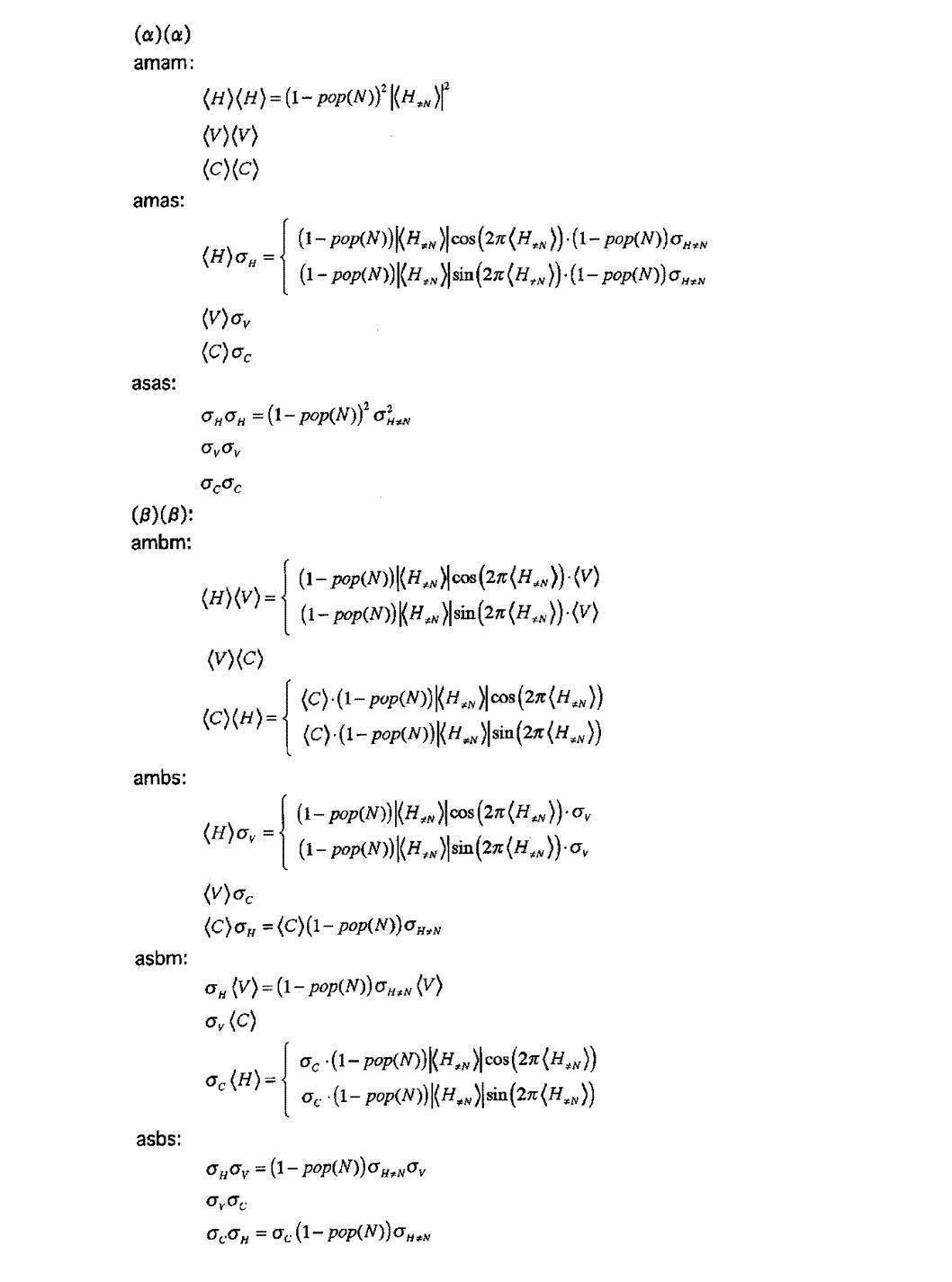
なお、エネルギーの要素の値は全て[-1,1]の範囲で記述される。
エネルギー要素Enとしては以下のものが定義される。
なお、エネルギーの要素の値は全て[-1,1]の範囲で記述される。
3-5.部分系の温度の計算
エネルギー要素の値をまとめてベクトル表記すると、部分系のエネルギーベクトルが定義できる。

部分系のエネルギーベクトルのノルムを計算すると部分系に関する画像の温度Tを定義できる。

エネルギー要素の値をまとめてベクトル表記すると、部分系のエネルギーベクトルが定義できる。
部分系のエネルギーベクトルのノルムを計算すると部分系に関する画像の温度Tを定義できる。
3-6.部分系の自由エネルギーの計算
このように算出されてきたエネルギー要素Enのベクトル、画像の温度T、エントロピーSの巨視的物理量を用いて、熱力学的不変量である自由エネルギーを定義する。自由エネルギーは、エネルギーベクトルに対してスカラー量を1つ加えたベクトルである。

このように算出されてきたエネルギー要素Enのベクトル、画像の温度T、エントロピーSの巨視的物理量を用いて、熱力学的不変量である自由エネルギーを定義する。自由エネルギーは、エネルギーベクトルに対してスカラー量を1つ加えたベクトルである。
ここに、<>は任意の一般画像に関する統計平均を表す。したがって、<S>は予め用意しておいた多量の任意の一般画像に関して、画像のエントロピーを計算し、それらの平均値を事前に算出しておく必要がある。物理的に1/<S>は、この部分系で規定されるプランク定数hに基づいて位相空間上の微視的状態数をエントロピーという巨視的物理量に結びつけるためのボルツマン定数kの役割を果たす。すなわち、位相空間上での状態数

(sは系の自由度の数)に対して、エントロピーはS=lnΔΓの関係で結ばれている(文献E3参照)。そして、温度をエネルギー量と結びつけるにはボルツマン定数kを介して、kTによって測られる。なお通常、ボルツマン定数はエントロピーの側に含めて定義し、温度はエネルギーと同じスケールの大きさで記述できるようにする定義が採用されることが多い(文献E7参照)。すなわち、S=klnΔΓ。画像系の量子状態は、部分系によってプランク定数の定義が変わるため、このような絶対的に不変な物理定数を定義できない。そこで、その部分系の中で一般画像がとりうる平均的な状態数を基準として、各々の画像がとっている状態数を絶対基準で計測するための規格化を行う操作をしている。これがボルツマン定数と同じ役割を果たす。この部分系のボルツマン定数は、下式で表すことができる。

[文献E7]ランダウ、リフシッツ理論物理学教程第5巻「統計物理学第1部」(第3版、1976年)、第2章「熱力学的諸量」、第9節「温度」
4.色の高次不変量の作成
この部分系を区別するための記号として不変量に対してFという記号を用いる場合がある。
4.色の高次不変量の作成
この部分系を区別するための記号として不変量に対してFという記号を用いる場合がある。
4-0.低次系の分布関数のヒルベルト空間表現
HVC面の色のヒストグラムを、色の低次系の分布関数と位置づける。低次系の分布関数は、元の座標系で測ることのできる座標空間qとも解釈することができる。これをチェビシェフ変換して周波数表現し、運動量空間pに投影する。これは元の分布関数を別の側面から見た等価表現である。ヒルベルト空間をなす基底関数として、低次系の分布関数の性質を加味して、できるだけコンパクトに表現する完全直交系の関数を選ぶ。しかし、座標空間と運動量空間の不確定性原理

によって、一方でコンパクト表現されているときは他方はブロードな表現となる関係にもある。その両者の不確定性が最小となるような関数系を選ぶのが最適である。
HVC面の色のヒストグラムを、色の低次系の分布関数と位置づける。低次系の分布関数は、元の座標系で測ることのできる座標空間qとも解釈することができる。これをチェビシェフ変換して周波数表現し、運動量空間pに投影する。これは元の分布関数を別の側面から見た等価表現である。ヒルベルト空間をなす基底関数として、低次系の分布関数の性質を加味して、できるだけコンパクトに表現する完全直交系の関数を選ぶ。しかし、座標空間と運動量空間の不確定性原理
によって、一方でコンパクト表現されているときは他方はブロードな表現となる関係にもある。その両者の不確定性が最小となるような関数系を選ぶのが最適である。
第1の実施形態と同様に、このとき展開係数の値が[-1,1]の範囲に収まるように定義されているものとする。

(α)がHのときx=H、(α)がVのときx=V、(α)がCのときx=Cである。Nの値はN=100とする。
(α)がHのときx=H、(α)がVのときx=V、(α)がCのときx=Cである。Nの値はN=100とする。
4-1.高次系の分布関数の作成
チェビシェフ展開された係数のパワースペクトルを、色に関する高次系の分布関数と定義する。H,V,C3面について、高次系の分布関数が定義できる。確率密度を表すように規格化しておく。

色の高次系の分布関数も2N=200のとき、kの値は200個のビンに量子化される。
チェビシェフ展開された係数のパワースペクトルを、色に関する高次系の分布関数と定義する。H,V,C3面について、高次系の分布関数が定義できる。確率密度を表すように規格化しておく。
色の高次系の分布関数も2N=200のとき、kの値は200個のビンに量子化される。
4-2.エントロピーの計算
分布関数f(k)からエントロピーSを計算する。分布関数の値が0のところは、その状態をとらないという意味で、積分区間から排除するものとする。分布関数の色面を(α)で区別して表すと、H,V,C面の各々の分布関数からエントロピーが算出され、それらの和が色の高次系に射影された部分系のエントロピーを表す。

この値をSFとする。
分布関数f(k)からエントロピーSを計算する。分布関数の値が0のところは、その状態をとらないという意味で、積分区間から排除するものとする。分布関数の色面を(α)で区別して表すと、H,V,C面の各々の分布関数からエントロピーが算出され、それらの和が色の高次系に射影された部分系のエントロピーを表す。
この値をSFとする。
4-3.運動量の要素pnの計算
チェビシェフ展開係数はヒルベルト空間における運動量と捉えることができる。したがって、運動量の要素pnは展開係数そのものである。
pn (α)=cn (α) (α)=H,V,C。
異なる色面の運動量についても順にpnでまとめて表すことにする。これらがこの部分系の位相空間の運動量p=(p1,p2,…,pi,…)を構成する。
チェビシェフ展開係数はヒルベルト空間における運動量と捉えることができる。したがって、運動量の要素pnは展開係数そのものである。
pn (α)=cn (α) (α)=H,V,C。
異なる色面の運動量についても順にpnでまとめて表すことにする。これらがこの部分系の位相空間の運動量p=(p1,p2,…,pi,…)を構成する。
4-4.エネルギーの要素Enの計算
運動量の積によって運動エネルギーを表すエネルギー行列を構築する際に、第5の実施形態では角運動量の単位で部分行列を作って、完全系をなすように拡張シュプールをとる。それによってエネルギーの固有値を求める。それらがエネルギーの要素となる。基本的に第1の実施形態と同じ要領でエネルギー不変量を構築する。
運動量の積によって運動エネルギーを表すエネルギー行列を構築する際に、第5の実施形態では角運動量の単位で部分行列を作って、完全系をなすように拡張シュプールをとる。それによってエネルギーの固有値を求める。それらがエネルギーの要素となる。基本的に第1の実施形態と同じ要領でエネルギー不変量を構築する。
エネルギーの要素を定義するとき、それらの各々が[-1,1]の範囲に収まるように、シュワルツの不等式で保証された関係を用いて、エネルギー行列の純粋なシュプール、すなわち対角要素の和で規格化しておく。したがって、純粋なシュプールのみで構築される定常状態のみが、規格化操作ができない。それ以外のエネルギー要素については全て規格化して拡張シュプールを定義する。純粋な対角和の値は、分布関数の展開係数の各々が[-1,1]の範囲で定義されることから、少々はみ出すことはあってもおよそ[0,1]の範囲の値が求まる。
エネルギー固有値は、絶対的なエネルギー量を表すので、最終的にこれらの線形結合をとるにあたっても、エネルギー固有値が有限の値を持っていることと、線形結合係数が零でない値を持っていることでは異なる意味をなす。エネルギー固有値は、その画像自体が発しているエネルギー要素の存在の有無を表し、線形結合係数は、ある形容詞にとって重要な要素か否かを表すだけである。したがって、エネルギー固有値は、絶対基準で計測されなければならない。上述の対角和が[0,1]の範囲を超えて少々はみ出すことがある問題については、元から対角和のエネルギーについては零点エネルギーε0が加わっていたものとして、零点エネルギーに相当する分を引き算して定義するようにしてもよい。零点エネルギーを導入しても線形結合係数に対しては何の影響も与えない。ここで、色の高次系のチェビシェフ展開係数の場合は、零点エネルギーとして1/3=0.333程度の値を導入する。また、後述するテキスチャの高次系の球ベッセル展開係数の場合は、対角和が[0,1]の範囲を超えないので、零点エネルギーを導入する必要はない。
以下では、cnを角運動量単位の部分群に分けて考える場合は、角運動量量子数l=0の展開係数をc0n、角運動量量子数l=1の展開係数をc1nと表すことにする。したがって、展開係数の要素数は半々のN個ずつに分かれる。部分群の要素番号はn=1,2,...,Nで数えるものとする。また、純粋な対角和を表す1つのエネルギー要素のみを別定義で与える。
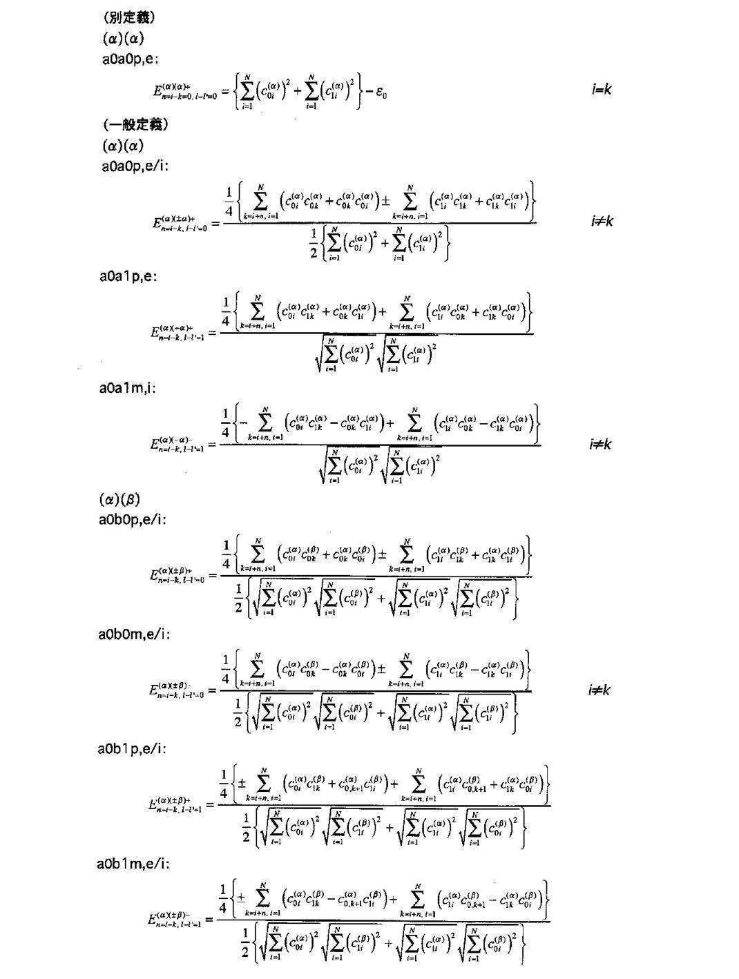
ここに、c0k=c0,N+nのような値をとった時、c0,N+n=c0,nのように同一角運動量の部分群内でベクトル{c0k}を円環につないで、最初の地点に戻って定義し直すものとする。同様にc1,N+n=c1,nである。これらのエネルギー要素をまとめてEnで表すことにする。
4-5.部分系の温度の計算
前述と同様にして、部分系のエネルギーベクトルと部分系の温度Tが定義できる。

前述と同様にして、部分系のエネルギーベクトルと部分系の温度Tが定義できる。
4-6.部分系の自由エネルギーの計算
前述と同様に、部分系の自由エネルギーが定義できる。

この部分系のボルツマン定数は、この部分系のエントロピーの任意の画像の統計平均の逆数で測る。

前述と同様に、部分系の自由エネルギーが定義できる。
この部分系のボルツマン定数は、この部分系のエントロピーの任意の画像の統計平均の逆数で測る。
5.テキスチャの低次不変量の作成
この部分系を区別するための記号として不変量に対してGoという記号を用いる場合がある。
5-1.低次系の分布関数の作成
第3の実施形態と同様に、ヒストグラムのビン数は200とする。分布関数はビンの単位で量子化されていて、それ以上の精度で記述できない。分布関数を同じく以下のように表す。
f(△H), f(△V), f(△C)
分布関数f(x)の変数x=△H,△V,△Cの値は、ビン数に関係なく、マンセル値で定義した上で、HVC間で等歩度性を満たすように微分値として[-1,1]に規格化しているものとする。
すなわち、
△H≡△H/100,
△V≡△V/10,
△C≡△C/20。
この部分系を区別するための記号として不変量に対してGoという記号を用いる場合がある。
5-1.低次系の分布関数の作成
第3の実施形態と同様に、ヒストグラムのビン数は200とする。分布関数はビンの単位で量子化されていて、それ以上の精度で記述できない。分布関数を同じく以下のように表す。
f(△H), f(△V), f(△C)
分布関数f(x)の変数x=△H,△V,△Cの値は、ビン数に関係なく、マンセル値で定義した上で、HVC間で等歩度性を満たすように微分値として[-1,1]に規格化しているものとする。
すなわち、
△H≡△H/100,
△V≡△V/10,
△C≡△C/20。
また、分布関数は規格化の条件を満たす。よって、確率密度を記述する。

5-2.エントロピーの計算
分布関数f(x)からエントロピーSを計算する。分布関数の値が0のところは、その状態をとらないという意味で、積分区間から排除するものとする。分布関数の色面を(α)で区別して表すと、H,V,C面の各々のエッジ画像の分布関数からエントロピーが算出され、それらの和がテキスチャの低次系に射影された部分系のエントロピーを表す。

この値をSGoとする。
分布関数f(x)からエントロピーSを計算する。分布関数の値が0のところは、その状態をとらないという意味で、積分区間から排除するものとする。分布関数の色面を(α)で区別して表すと、H,V,C面の各々のエッジ画像の分布関数からエントロピーが算出され、それらの和がテキスチャの低次系に射影された部分系のエントロピーを表す。
この値をSGoとする。
5-3.運動量の要素pnの計算
分布関数f(x)から平均値<x>と標準偏差値σxを計算する。

x=△H,△V,△Cであるので、それぞれを運動量の要素pnとして対応させる。
<△H>, <△V>, <△C>, σ△H, σ△V, σ△C
なお、運動量の要素の値は全て[-1,1]の範囲で記述される。
分布関数f(x)から平均値<x>と標準偏差値σxを計算する。
x=△H,△V,△Cであるので、それぞれを運動量の要素pnとして対応させる。
<△H>, <△V>, <△C>, σ△H, σ△V, σ△C
なお、運動量の要素の値は全て[-1,1]の範囲で記述される。
5-4.エネルギーの要素Enの計算
エネルギー要素Enとしては以下のものが定義される。これらの値は全て実数で定義される。
(α)(α)
amam:
<△H><△H>
<△V><△V>
<△C><△C>
amas:
<△H>σ△H
<△V>σ△V
<△C>σ△C
asas:
σ△Hσ△H
σ△Vσ△V
σ△Cσ△C
(β)(β):
ambm:
<△H><△V>
<△V><△C>
<△C><△H>
ambs:
<△H>σ△V
<△V>σ△C
<△C>σ△H
asbm:
σ△H<△V>
σ△V<△C>
σ△C<△H>
asbs:
σ△Hσ△V
σ△Vσ△C
σ△Cσ△H
なお、エネルギーの要素の値は全て[-1,1]の範囲で記述される。
5-5.部分系の温度の計算
前述と同様にして、部分系のエネルギーベクトルと部分系の画像の温度Tが定義できる。
5-6.部分系の自由エネルギーの計算
前述と同様に、部分系の自由エネルギーが定義できる。

前述と同様にして、部分系のエネルギーベクトルと部分系の画像の温度Tが定義できる。
5-6.部分系の自由エネルギーの計算
前述と同様に、部分系の自由エネルギーが定義できる。
この部分系のボルツマン定数は、この部分系のエントロピーの任意の画像の統計平均の逆数で測る。

6.テキスチャの高次不変量の作成
この部分系を区別するための記号として不変量に対してGという記号を用いる場合がある。
6-0.低次系の分布関数のヒルベルト空間表現
HVC面のエッジ画像のヒストグラムを、テキスチャの低次系の分布関数と位置づける。低次系の分布関数は、元の座標系で測ることのできる座標空間qとも解釈することができる。これを球ベッセル変換して周波数表現し、運動量空間pに投影する。これは元の分布関数を別の側面から見た等価表現である。ヒルベルト空間をなす基底関数として、低次系の分布関数の性質を加味して、できるだけコンパクトに表現する完全直交系の関数を選ぶ。しかし、座標空間と運動量空間の不確定性原理

によって、一方でコンパクト表現されているときは他方はブロードな表現となる関係にもある。その両者の不確定性が最小となるような関数系を選ぶのが最適である。
この部分系を区別するための記号として不変量に対してGという記号を用いる場合がある。
6-0.低次系の分布関数のヒルベルト空間表現
HVC面のエッジ画像のヒストグラムを、テキスチャの低次系の分布関数と位置づける。低次系の分布関数は、元の座標系で測ることのできる座標空間qとも解釈することができる。これを球ベッセル変換して周波数表現し、運動量空間pに投影する。これは元の分布関数を別の側面から見た等価表現である。ヒルベルト空間をなす基底関数として、低次系の分布関数の性質を加味して、できるだけコンパクトに表現する完全直交系の関数を選ぶ。しかし、座標空間と運動量空間の不確定性原理
によって、一方でコンパクト表現されているときは他方はブロードな表現となる関係にもある。その両者の不確定性が最小となるような関数系を選ぶのが最適である。
第3の実施形態と同様に、本実施形態では、s,p軌道による展開の場合の説明を行う。なお、s,p,d,f軌道による展開の場合も、冒頭説明したように同様に展開していくことができる。

(α)がHのときx=△H、(α)がVのときx=△V、(α)がCのときx=△Cである。Nの値はN=100とする。
(α)がHのときx=△H、(α)がVのときx=△V、(α)がCのときx=△Cである。Nの値はN=100とする。
6-1.高次系の分布関数の作成
球ベッセル展開された係数のパワースペクトルを、テキスチャに関する高次系の分布関数と定義する。H,V,C3面について、高次系の分布関数が定義できる。確率密度を表すように規格化しておく。

球ベッセル展開された係数のパワースペクトルを、テキスチャに関する高次系の分布関数と定義する。H,V,C3面について、高次系の分布関数が定義できる。確率密度を表すように規格化しておく。
テキスチャの高次系の分布関数はN=100のとき、1つの角運動量につき、kの値は100個のビンに量子化される。lの値は0と1をとるから合計で2x100=200個のビンに量子化される。
6-2.エントロピーの計算
分布関数f(l,k)からエントロピーSを計算する。分布関数の値が0のところは、その状態をとらないという意味で、積分区間から排除するものとする。分布関数の色面を(α)で区別して表すと、H,V,C面の各々のエッジ画像の分布関数からエントロピーが算出され、それらの和がテキスチャの高次系に射影された部分系のエントロピーを表す。

この値をSGとする。
分布関数f(l,k)からエントロピーSを計算する。分布関数の値が0のところは、その状態をとらないという意味で、積分区間から排除するものとする。分布関数の色面を(α)で区別して表すと、H,V,C面の各々のエッジ画像の分布関数からエントロピーが算出され、それらの和がテキスチャの高次系に射影された部分系のエントロピーを表す。
この値をSGとする。
6-3.運動量の要素pnの計算
球ベッセル展開係数はヒルベルト空間における運動量と捉えることができる。したがって、運動量の要素pnは展開係数そのものである。
pn (α)=c0n (α)
pN+n (α)=c1n (α) (α)=H,V,C。
異なる色面の運動量についても順にpnでまとめて表すことにする。これらがこの部分系の位相空間の運動量p=(p1,p2,…,pi,…)を構成する。
球ベッセル展開係数はヒルベルト空間における運動量と捉えることができる。したがって、運動量の要素pnは展開係数そのものである。
pn (α)=c0n (α)
pN+n (α)=c1n (α) (α)=H,V,C。
異なる色面の運動量についても順にpnでまとめて表すことにする。これらがこの部分系の位相空間の運動量p=(p1,p2,…,pi,…)を構成する。
6-4.エネルギーの要素Enの計算
s,p軌道までの展開のときは、色の高次系であるチェビシェフ展開係数について定義した式と全く同様である。チェビシェフ展開係数を球ベッセル展開係数に置き換えるだけでよい。なお、テキスチャの高次系の場合は、零点エネルギーにつてはε0=0と置いてよい。
s,p軌道までの展開のときは、色の高次系であるチェビシェフ展開係数について定義した式と全く同様である。チェビシェフ展開係数を球ベッセル展開係数に置き換えるだけでよい。なお、テキスチャの高次系の場合は、零点エネルギーにつてはε0=0と置いてよい。
6-5.部分系の温度の計算
前述と同様にして、部分系のエネルギーベクトルと部分系の画像の温度Tが定義できる。
6-6.部分系の自由エネルギーの計算
前述と同様に、部分系の自由エネルギーが定義できる。

前述と同様にして、部分系のエネルギーベクトルと部分系の画像の温度Tが定義できる。
6-6.部分系の自由エネルギーの計算
前述と同様に、部分系の自由エネルギーが定義できる。
この部分系のボルツマン定数は、この部分系のエントロピーの任意の画像の統計平均の逆数で測る。

7.部分系の形容詞エネルギーへの統合
7-1.形容詞の設定
形容詞をキーワードとする感性検索システムで提示する形容詞を決め、それらを区別するための記号として、i番目の形容詞と割り当てる。形容詞として、例えば、「爽やかな」、「賑やかな」、「荒々しい」、「しっとりとした」などである。
7-1.形容詞の設定
形容詞をキーワードとする感性検索システムで提示する形容詞を決め、それらを区別するための記号として、i番目の形容詞と割り当てる。形容詞として、例えば、「爽やかな」、「賑やかな」、「荒々しい」、「しっとりとした」などである。
7-2.一般画像モデルの構築
任意の一般画像を多数枚ランダムに集めて、それらを一般画像のモデルとする。通常、数百枚以上のオーダーの画像を用意する。更に正確を期するならば万のオーダーとなり、多ければ多いほど統計が安定する。これらを用いて以下に述べる一般モデル画像群の分布関数p(x)を構築する。分布関数p(x)は実数値Enのとる単位エネルギー区間内で一般画像がとりうる画像頻度を表し、エネルギー区間をビンとして区切れば、度数分布関数となる。
任意の一般画像を多数枚ランダムに集めて、それらを一般画像のモデルとする。通常、数百枚以上のオーダーの画像を用意する。更に正確を期するならば万のオーダーとなり、多ければ多いほど統計が安定する。これらを用いて以下に述べる一般モデル画像群の分布関数p(x)を構築する。分布関数p(x)は実数値Enのとる単位エネルギー区間内で一般画像がとりうる画像頻度を表し、エネルギー区間をビンとして区切れば、度数分布関数となる。
7-3.形容詞モデル画像の構築
上記用意した一般画像モデルの各々に対し、i番目の形容詞に該当するか否かの心理的な印象評価を行い、形容詞モデル画像の分布データを作成する。この作成方法には2通りがあり、どちらを使ってもよい。すなわち、単なる該当、非該当の場合は1、0の整数を割り振り、1が割り当てられた画像を、同じ重みの画像として用いる。そして、該当画像群を用いて形容詞モデル画像群の分布関数q(x)を構築する。もう1つは、非該当の場合を0とし、該当の場合の心理的な絶対印象度合いを1-5の5段階評価をする方法である。この場合には、モデルの分布データを構築するに当たり、5評価の画像には1.0の重みを、4評価の画像には0.8の重みを、3評価の画像には0.6の重みを、2評価の画像には0.4の重みを、1評価の画像には0.2の重みをつけて以下に述べる度数分布q(x)を構築する。
上記用意した一般画像モデルの各々に対し、i番目の形容詞に該当するか否かの心理的な印象評価を行い、形容詞モデル画像の分布データを作成する。この作成方法には2通りがあり、どちらを使ってもよい。すなわち、単なる該当、非該当の場合は1、0の整数を割り振り、1が割り当てられた画像を、同じ重みの画像として用いる。そして、該当画像群を用いて形容詞モデル画像群の分布関数q(x)を構築する。もう1つは、非該当の場合を0とし、該当の場合の心理的な絶対印象度合いを1-5の5段階評価をする方法である。この場合には、モデルの分布データを構築するに当たり、5評価の画像には1.0の重みを、4評価の画像には0.8の重みを、3評価の画像には0.6の重みを、2評価の画像には0.4の重みを、1評価の画像には0.2の重みをつけて以下に述べる度数分布q(x)を構築する。
7-4.要素内の分布における偏差値の算出
上記定義してきた部分系の各々のエネルギー要素Enについて1つ1つ個別に、一般モデル画像がとるEnの値の分布と形容詞モデル画像がとるEnの値の分布とを調べ、形容詞モデル画像が一般モデル画像の平均とは異なる位置に分布しているとき、そのエネルギー要素はその形容詞にとって特異な働きをしているものとして、エネルギー和をとるときの線形結合係数の形で、その重みを与える。その特異な働きの具合は、一般モデル画像の分布に対して、形容詞モデル画像の分布が位置している偏差値で与えることができる。
上記定義してきた部分系の各々のエネルギー要素Enについて1つ1つ個別に、一般モデル画像がとるEnの値の分布と形容詞モデル画像がとるEnの値の分布とを調べ、形容詞モデル画像が一般モデル画像の平均とは異なる位置に分布しているとき、そのエネルギー要素はその形容詞にとって特異な働きをしているものとして、エネルギー和をとるときの線形結合係数の形で、その重みを与える。その特異な働きの具合は、一般モデル画像の分布に対して、形容詞モデル画像の分布が位置している偏差値で与えることができる。
エネルギー要素Enを変数xで表し、一般モデル画像の分布関数がp(x)、形容詞モデル画像の分布関数がq(x)であるとする。一般モデル画像のエネルギー要素Enの平均値をmp、その標準偏差σp、形容詞モデル画像のエネルギー要素Enの平均値をmq、その標準偏差σqとする。そのとき、i番目の形容詞に対応するエネルギー要素Enに対する線形結合係数αi(En)は、誤差関数erf(x)を用いて以下のように表すことができる。線形結合係数は、一般モデル画像の平均値と同じところに位置するときは0、両端に位置するときは±1となるように定義する。また、形容詞モデル画像群の偏差値のゆらぎ、すなわち線形結合係数の誤差δαi(En)も評価できる。
各エネルギー要素Enに対して
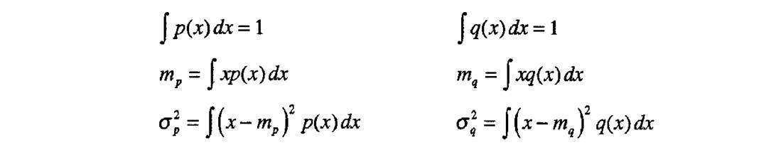
偏差値およびその誤差
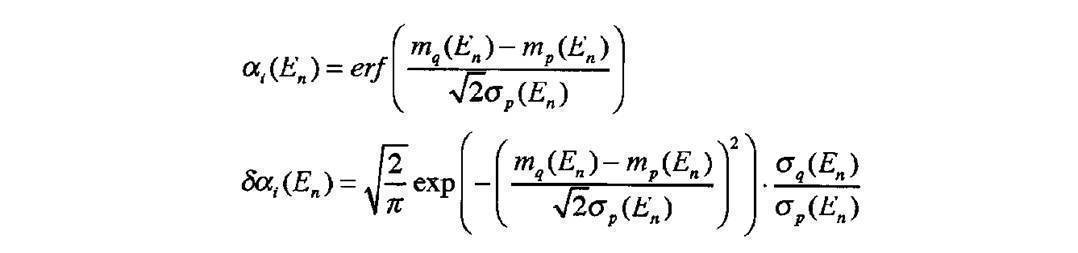
ここに、

であり、erf(±∞)=±1、erf(0)=0の値を返す。
であり、erf(±∞)=±1、erf(0)=0の値を返す。
7-5.部分系単位の部分エネルギーの算出
ある画像を入力し、それがi番目の形容詞の印象を備えているか否かを調べるために、その入力された画像に対して、各部分系のエネルギー要素を算出し、形容詞モデルによって確定された線形結合係数を用いて、その形容詞エネルギーの絶対量の総和を求める。その総和を求めるに当たって、まず部分系単位で部分和をとる。ここに部分系の自由エネルギーベクトルに対して、線形結合係数をベクトル表記したモデル形容詞ベクトルとの内積をとって部分和を定義する。そのとき、自由エネルギーとして熱量-TSというスカラー量を1つ付け加えた成分に対しても、対応する線形結合係数を定義する。すなわち、
自由エネルギーベクトル

ある画像を入力し、それがi番目の形容詞の印象を備えているか否かを調べるために、その入力された画像に対して、各部分系のエネルギー要素を算出し、形容詞モデルによって確定された線形結合係数を用いて、その形容詞エネルギーの絶対量の総和を求める。その総和を求めるに当たって、まず部分系単位で部分和をとる。ここに部分系の自由エネルギーベクトルに対して、線形結合係数をベクトル表記したモデル形容詞ベクトルとの内積をとって部分和を定義する。そのとき、自由エネルギーとして熱量-TSというスカラー量を1つ付け加えた成分に対しても、対応する線形結合係数を定義する。すなわち、
自由エネルギーベクトル
モデル形容詞ベクトル

部分系をa1,a2,...のように区別するインデックスを付けて部分系単位のエネルギー和Piを内積によって求める。a1は色の低次系、a2は色の高次系、a3はテキスチャの低次系、a4はテキスチャの高次系などと対応する。

しかしながら、これらの線形結合をとって、全形容詞エネルギーQiを求めるにあたって、上述の単なる内積では、定義しうるエネルギー要素の数が多い系ほどPiの値は大きな値をとってしまう。部分系は独立な側面を記述しており、部分系の統合を行う時点では、均等な扱いをする必要がある。そのために部分和Piの値がおよそ[-1,1]の範囲に入るように規格化をしておく必要がある。すなわち、
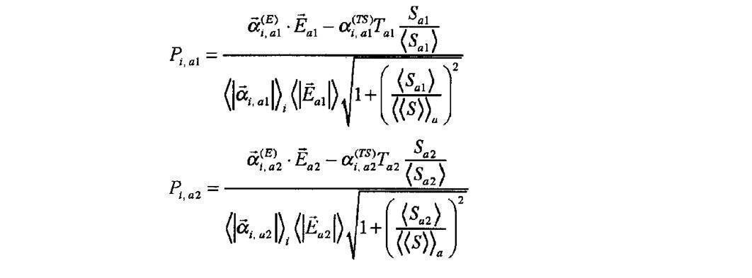
ここに<>aは全ての部分系の間に関する統計平均を表す。すなわち、考察した部分系の数をnaとすると、

ここでも分母の規格化においては可能な限り統計平均を行うべきであるという考え方に準じている。これによって、部分系によって違って定義される分布関数の量子化のビン数の違いによる状態数の違い、すなわちエントロピーの違いは吸収され、異なる部分系を共通土俵に乗せることができる。すなわち、部分系によって異なるプランク定数やボルツマン定数の定義がここで吸収され、同等の扱いをすることができるスケールのエネルギー物理量Piが算出される。物理的には分母の平方根の項は、部分系によって物理定数が異なるときに必要になる補正項と解することができる。一方の平均温度や形容詞ベクトルのノルム平均は、部分系によって定義しうるエネルギー要素の数の違いを吸収するための規格化である。このように部分系を共通土俵に乗せるためのノルムの統計平均量による規格化は、絶対物理量を規定する上で極めて重要な役割を果たす。
参考のために、任意の一般画像を多量に用意して、それらのエントロピーの値と温度の値をそれぞれの部分系について実験的に調べた結果を示す。これらの数値を見れば、規格化の手続きが部分系を統合する上で如何に重要であるかがわかる。
エントロピー
7.97≦~SFo≦~14.30 <SFo>=12.51
2.49≦ ~SF≦~6.05 <SF>=4.67
8.75≦ ~SGo≦~14.39 <SGo>=12.19
7.49≦ ~SG≦~13.82 <SG>=10.81
温度
0.18≦ ~TFo≦~1.37 <TFo>=0.73
2.68≦ ~TF≦~3.31 <TF>=2.91
0.003≦ ~TGo≦~0.10 <TGo>=0.03
5.75≦ ~TG≦~20.63 <TG>=12.31
したがって、1/<S>~0.1のオーダーの数値であり、分母の平方根は1.1~1.6程度の値である。
8.全系の形容詞エネルギーへの統合
次に部分系のエネルギーを統合する。全系の形容詞エネルギーQiを求めるために、部分和エネルギーPiを線形結合する。このときの線形結合係数は、ある形容詞iにとって色の低次系、色の高次系、テキスチャの低次系、テキスチャの高次系などの何れが重要な役割を占めているかを決めることになる。更に部分系として構図を加えたときは、構図の要素の重要度も加味されることになる。
次に部分系のエネルギーを統合する。全系の形容詞エネルギーQiを求めるために、部分和エネルギーPiを線形結合する。このときの線形結合係数は、ある形容詞iにとって色の低次系、色の高次系、テキスチャの低次系、テキスチャの高次系などの何れが重要な役割を占めているかを決めることになる。更に部分系として構図を加えたときは、構図の要素の重要度も加味されることになる。
線形結合係数を決定するためのステップは、前述の1つ1つのエネルギー要素Enに対してαiを決定するために行ったのと同様の手続きにより行われる。すなわち、部分和Pi,jを変数xとして、一般モデル画像の分布に対して平均値をmp、その標準偏差σp、形容詞モデル画像の分布に対して平均値をmq、その標準偏差σqを求め、同様に線形結合係数を決定する。
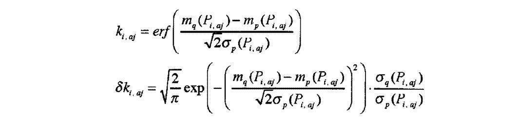
これらの線形結合係数を用いて、形容詞iに関する全系のエネルギー和Qiを求める。このときもおよそ[-1,1]の範囲に収まるように規格化を行っておく。

ここに<>は一般モデル画像に関する平均、<>iは形容詞に関する平均を表す。なお、これまでに示したエネルギーバンド図はこの部分系の重み係数kについても内包する形のα(En)を用いて描いた図である。また、状態密度については一般モデル画像に用いたエネルギー要素の中でプラスマイナスに最大に振れるガマット領域ρmax(En)に対して、α(En)ρmax(En)として最大考慮される範囲をエネルギーバンドモデルとして塗りつぶしている。
9.形容詞検索処理
このように学習用として一般モデルと形容詞モデルを組んで、エネルギーバンドモデルを構築すると、別のデータベースの画像に対して、i番目の形容詞をキーワードとして、それに近い印象の画像を形容詞エネルギーQiに基づいて検索をすることができる。Qiの順に画像を並べると、またそれは正規分布に近い形となり、上位群の偏差値の高い領域を目的の画像として提示することができる。また、更には下位群の偏差値が低い領域をこの形容詞とは反対構造をもった印象の画像であるとして提示することもできる。すなわち、ユーザーとしては反対の意味の感性画像の分類結果についても知ることができる。
このように学習用として一般モデルと形容詞モデルを組んで、エネルギーバンドモデルを構築すると、別のデータベースの画像に対して、i番目の形容詞をキーワードとして、それに近い印象の画像を形容詞エネルギーQiに基づいて検索をすることができる。Qiの順に画像を並べると、またそれは正規分布に近い形となり、上位群の偏差値の高い領域を目的の画像として提示することができる。また、更には下位群の偏差値が低い領域をこの形容詞とは反対構造をもった印象の画像であるとして提示することもできる。すなわち、ユーザーとしては反対の意味の感性画像の分類結果についても知ることができる。
更には、ある一枚の画像を入力し、予め用意した形容詞モデルの形容詞全てについてQiを計算しておけば、そのモデルとなった人物にとって、その画像から受ける絶対印象の度合いを、全ての形容詞について数値化することができる。これを値の大きい順に並び替えて表示すれば、この画像は「爽やかさ」が0.8で「のどかさ」も0.7と高く、「賑やかさ」は-0.7と反対方向に低いためその印象は全く感じないといった結果を提示することができる。
形容詞のエネルギーバンドモデルとしては、万人に共通する平均モデルにとることもでき、国、文化、言語の違いに応じてそれらの文化圏に特有のモデルを構築することもできる。あるいは、個人レベルの嗜好の違いを反映した個性的なエネルギーバンドモデルも構築することができる。したがって、この画像検索システムが採用するエネルギーバンド構造のモデルは、人の感性の構造を定量的に解明するツールとしても使うことができる。
実験的に、個性の違いが区別できるか試してみたところ、「荒々しい」という形容詞に対して、一人目は山肌の木々が鋭く林立した風景と川の流れが激しくしぶきを上げる様子と半々程度に選んだモデルに対して、感性検索結果はそれらの要素を複合的に捉えて上位群に集めてくる効果を示した。また、別の人は川の流れが激しくしぶきを上げる様子を主なモデル画像として選んだのに対しては、形容詞エネルギーQiはきっちりと川の流れの特徴をつかんで、モデルに近い画像を抽出する性能を示した。ゆえに、特徴量として用いたエネルギー要素Enは、画像全体に写り込んだ物体を識別する能力を備えているということができる。
なお、偏差値によって線形結合係数を求める考え方を延長して、最終的に求めたQiの値が、一般モデル画像に対して形容詞モデル画像は、上位群に集まってきているか否かは、もう一度モデル画像群のQiの一般モデルに対する偏差値を求めておけば確認することができる。これによって、理論モデルの正当性と扱う特徴量の十分性を検証することができる。
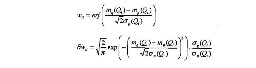
この考え方を拡張して、最終的に求めた各々の形容詞に関するQiに対して、j番目の形容詞エネルギーQjの一般モデル画像分布に対して、i番目の形容詞エネルギーQiの形容詞モデル画像分布がどこに位置しているかを見ることによって、j番目の形容詞にとってi番目の形容詞の絶対印象がどれだけ含まれているかが分かり、i番目の形容詞はj番目の形容詞と近い印象を与える同類群に属するような形容詞なのか、あるいはi番目の形容詞はj番目の形容詞と正反対の印象を与える遠くはなれた形容詞群に属する形容詞なのかを表現する形容詞間の相関行列wijを求めることができる。これにより、万人に共通の形容詞構造のマップが明らかになるとともに、文化圏の違いや、個性の違いに関する形容詞のマップ構造も解明することができる。
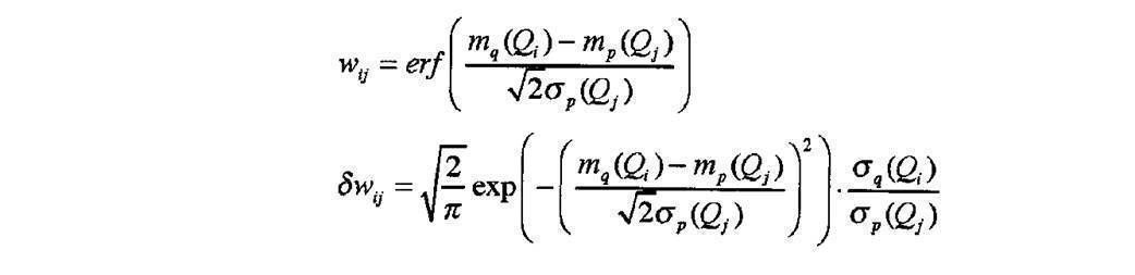
iとjの関係を入れ替えて、i番目の形容詞エネルギーQiの一般モデル分布画像に対して、j番目の形容詞エネルギーQjの形容詞モデル画像分布の偏差値も同様に別経路で計算することができる。定義からして形容詞の相関行列は対称行列である。すなわち、
wij = wji
しかしながら、別経路をたどって計算したものは、母集団画像の性質に偏りがある場合等には必ずしも一致しない。したがって、形容詞の相関行列が対称行列に近い値を示すか否かは、モデル構築過程に選んだ画像群が一般性の高いランダムな画像を選定しているか否かに関する妥当性を検証するためのよい指標を与える。また、対角成分は前述したように全てが1になるのが望ましく、そこに到達していない場合は、その形容詞を捉えるための特徴量が不足しているか、理論モデル仮説の成り立たない部分が存在することを意味するので、検索システムを構築する上でよい評価指標を与える。
wij = wji
しかしながら、別経路をたどって計算したものは、母集団画像の性質に偏りがある場合等には必ずしも一致しない。したがって、形容詞の相関行列が対称行列に近い値を示すか否かは、モデル構築過程に選んだ画像群が一般性の高いランダムな画像を選定しているか否かに関する妥当性を検証するためのよい指標を与える。また、対角成分は前述したように全てが1になるのが望ましく、そこに到達していない場合は、その形容詞を捉えるための特徴量が不足しているか、理論モデル仮説の成り立たない部分が存在することを意味するので、検索システムを構築する上でよい評価指標を与える。
[第6の実施形態]
(感性検索:「エネルギー+運動量+角運動量」の3段階統合)
第5の実施形態では、個性を反映した形容詞検索も可能であると述べた。しかし、個人の形容詞モデルを構築するに当たっては、ある程度多くの画像が用意されていることが望ましい。それに対して、もっと少数の3~5枚程度の画像を提示して、それらの画像感性に近い画像をデータベースから選び出したいというような目的のときには、統計平均による情報の消失過程が不完全状態となるので、第5の実施形態で省略した力学的不変量も考察対象に加える必要が生じる。それに伴って新たに付け加える過程だけ以下に述べる。
(感性検索:「エネルギー+運動量+角運動量」の3段階統合)
第5の実施形態では、個性を反映した形容詞検索も可能であると述べた。しかし、個人の形容詞モデルを構築するに当たっては、ある程度多くの画像が用意されていることが望ましい。それに対して、もっと少数の3~5枚程度の画像を提示して、それらの画像感性に近い画像をデータベースから選び出したいというような目的のときには、統計平均による情報の消失過程が不完全状態となるので、第5の実施形態で省略した力学的不変量も考察対象に加える必要が生じる。それに伴って新たに付け加える過程だけ以下に述べる。
1.マンセルHVC色空間への変換
2.HVC面のエッジ画像の作成
3.色の低次不変量の作成
3-1.低次系の分布関数の作成
3-2.エントロピーの計算
3-3.運動量の要素pnの計算
第5の実施形態で定義した運動量の内、平均値<H>、<V>、<C>のみを運動量の要素とする。
3-4.角運動量の要素Mnの計算
第5の実施形態で定義した運動量の内、標準偏差値σH、σV、σCを角運動量の要素とする。
3-5.エネルギーの要素Enの計算
3-6.部分系の温度の計算
色の高次系で後述する内容と同じ手続きを踏む。ここでは詳細を述べない。
3-7.部分系の自由エネルギーの計算
色の高次系で後述する内容と同じ手続きを踏む。ここでは詳細を述べない。
4.色の高次不変量の作成
4-0.低次系の分布関数のヒルベルト空間表現
4-1.高次系の分布関数の作成
4-2.エントロピーの計算
4-3.運動量の要素pnの計算
4-4.角運動量の要素Mnの計算
チェビシェフ展開係数は角運動量量子数l=0と1に分かれるから、角運動量量子数と運動量の積をとって角運動量を計算する。角運動量の要素Mnは次のようになる。
(c11 (α)+c12 (α)+...+c1N (α)) (α)=H,V,C。
4-5.エネルギーの要素Enの計算
4-6.部分系の温度の計算
エネルギー要素の値をエネルギーの単位でまとめてベクトル表記し、同様に運動量の要素の値も運動量の単位で、角運動量の要素の値も角運動量の単位でまとめてベクトル表記すると、部分系のエネルギーベクトルと運動量ベクトルと角運動量ベクトルが定義できる。
部分系のエネルギーベクトル、運動量ベクトル、角運動量ベクトルのそれぞれのノルムを計算すると、部分系に関する画像の温度TE,Tp,TMが力学的不変量の単位で定義できる。

4-7.部分系の自由エネルギーの計算
エネルギーの場合の類推から、部分系の自由エネルギー、自由運動量、自由角運動量を定義する。
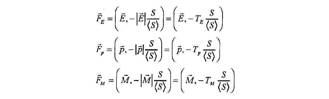
エネルギーの場合の類推から、部分系の自由エネルギー、自由運動量、自由角運動量を定義する。
5.テキスチャの低次不変量の作成
「3.色の低次不変量の作成」で述べた要領と全く同様である。
6.テキスチャの高次不変量の作成
s,p軌道による球ベッセル展開を行うときは、「4.色の高次不変量の作成」で述べた要領と全く同様であるので記述は省略する。
7.部分系の力学的不変量単位の統合
7-1.形容詞の設定
7-2.一般画像モデルの構築
7-3.形容詞モデル画像の構築
7-4.要素内の分布における偏差値の算出
第5の実施形態では各エネルギー要素Enについて偏差値とその誤差の算出を行ったが、第6の実施形態では同様のことを運動量の要素pnと角運動量の要素Mnについても行う。記号を変えて、エネルギー要素に対する偏差値をβi、運動量の要素に対する偏差値をγi、角運動量の要素に対する偏差値をδiとする。
7-5.部分系の力学的不変量単位の部分エネルギー、部分運動量、部分角運動量の算出
上述のようにして、自由エネルギーベクトル、自由運動量ベクトル、自由角運動量ベクトルの各々に対してモデル形容詞ベクトルが定まる。なお、TS不変量に対しても同様の過程を経て偏差値を定めているものとする。すなわち、
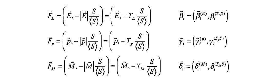
上述のようにして、自由エネルギーベクトル、自由運動量ベクトル、自由角運動量ベクトルの各々に対してモデル形容詞ベクトルが定まる。なお、TS不変量に対しても同様の過程を経て偏差値を定めているものとする。すなわち、
両者の内積をとって形容詞iの印象に関する部分系の力学的不変量単位の部分エネルギーEi、部分運動量pi、部分角運動量Miに統合する。規格化によって、全ての力学的不変量の次元が揃う。
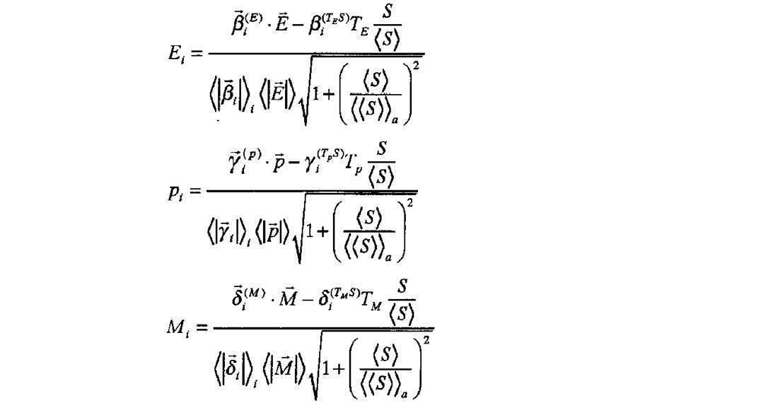
8.部分系の形容詞エネルギーへの統合
部分系の中で求まった3つの力学的不変量は、部分系内における形容詞iに関する統計平均されたエネルギーの期待値、運動量の期待値、角運動量の期待値を表す。それらの巨視的な物理量のうち、少数画像モデルの場合、どれが重要な役割を果たすかを、3つの力学的不変量を線形結合するときの結合係数によって表す。それらの結合係数は同様に、一般モデル画像と形容詞モデル画像の分布関数の位置関係から偏差値によって記述することができる。各々の結合係数をαi(Ei),αi(pi),αi(Mi)によって表す。
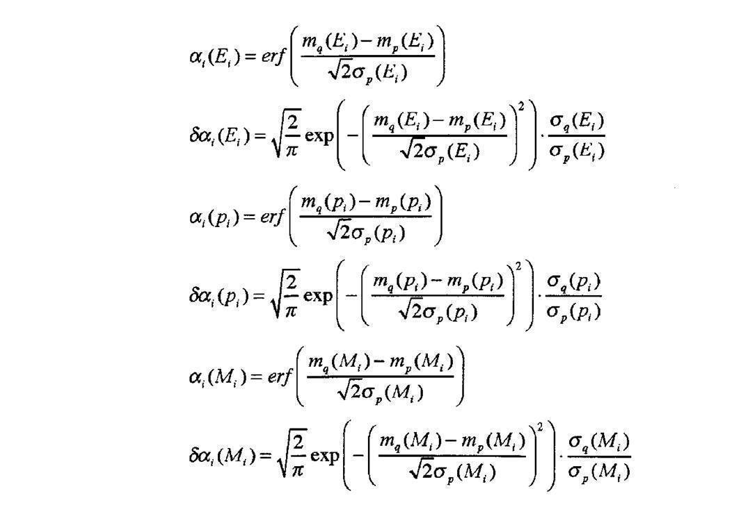
部分系の中で求まった3つの力学的不変量は、部分系内における形容詞iに関する統計平均されたエネルギーの期待値、運動量の期待値、角運動量の期待値を表す。それらの巨視的な物理量のうち、少数画像モデルの場合、どれが重要な役割を果たすかを、3つの力学的不変量を線形結合するときの結合係数によって表す。それらの結合係数は同様に、一般モデル画像と形容詞モデル画像の分布関数の位置関係から偏差値によって記述することができる。各々の結合係数をαi(Ei),αi(pi),αi(Mi)によって表す。
3つの線形結合係数をαiのベクトルとして、3つの力学的不変量をE'のベクトルとして表記する。

部分系の形容詞エネルギーPiはこれらの内積をとって表される。

9.全系の形容詞エネルギーへの統合
後は第5の実施形態と全く同様である。
10.形容詞検索処理
[第7の実施形態]
(一枚画像の類似画像検索:「エネルギー+運動量+角運動量」の3段階統合)
第6の実施形態では、少数モデルによる形容詞モデルを構築する例を示した。これを極限にまで持って行けば、一枚の類似画像検索に使うことができる。すなわち、例示された一枚の画像の全体の印象が近い画像を、巨視的な物理量であるエネルギー、運動量、角運動量の記述を通して抽出することが可能になる。
後は第5の実施形態と全く同様である。
10.形容詞検索処理
[第7の実施形態]
(一枚画像の類似画像検索:「エネルギー+運動量+角運動量」の3段階統合)
第6の実施形態では、少数モデルによる形容詞モデルを構築する例を示した。これを極限にまで持って行けば、一枚の類似画像検索に使うことができる。すなわち、例示された一枚の画像の全体の印象が近い画像を、巨視的な物理量であるエネルギー、運動量、角運動量の記述を通して抽出することが可能になる。
第6の実施形態の方法は、第5の実施形態の方法を包含している。なぜならば、モデル画像が多数になると、運動量と角運動量の役割が減って、自動的に統計平均によって、それらの線形結合係数は零に近い値に収束するからである。したがって、第6の実施形態の方法は、一枚画像検索から少数モデルの感性検索、更には多数モデルの感性検索までシームレスに実現することができる。
<均等認識空間への射影>
これまでの実施形態で定義してきた一次元の分布関数から導いた運動量、角運動量、エネルギーという概念についてもう一度、人間の認識の関わりの観点から議論する。
これまで低次系、高次系と呼んでいたのは、前者がマンセル色空間で表される実空間記述を表し、後者がマンセル値で表される実空間の分布関数を基底関数を用いて周波数空間に投影した周波数空間記述を表す。
これまでの実施形態で定義してきた一次元の分布関数から導いた運動量、角運動量、エネルギーという概念についてもう一度、人間の認識の関わりの観点から議論する。
これまで低次系、高次系と呼んでいたのは、前者がマンセル色空間で表される実空間記述を表し、後者がマンセル値で表される実空間の分布関数を基底関数を用いて周波数空間に投影した周波数空間記述を表す。
マンセル色空間は知覚的な等歩度性が保証された均等色空間である。従って、実空間記述におけるマンセル値そのものは空間の一様性が保証された色空間を提供している。他方、一次元ヒストグラムなどの形状を認識するとき、そのヒストグラムの分布関数が満たすべき拘束条件が存在し、人間はその拘束条件を加味した上で、自由度の存在する部分の形状の違いを認識する。その拘束条件と同じ性質を備える基底関数を用いて周波数展開すると、その展開係数は自由度の存在する部分の形状の違いを均等に認識する空間へ変換していると位置づけることができる。すなわち、周波数空間記述における基底関数空間は、空間の一様性が保証された認識空間を提供している。
従って、知覚的な色の認識の一様性を保証するマンセル色空間が提供する実空間も、分布関数の形状認識の一様性を保証する基底関数のヒルベルト空間が提供する周波数空間も、一様な認識を保証した均等認識空間をなしていると見なすことができる。すなわちマンセル色空間は「色の知覚」における均等認識空間を、ヒルベルト空間は「形の認識」における均等認識空間を提供する。
物理学では、「空間の一様性」から「運動量の保存則」が導かれる。更に「空間の等方性」から「角運動量の保存則」が導かれ、「時間の一様性」から「エネルギーの保存則」が導かれる(文献A2-2参照)。
これを画像系に対応させると画像認識において、実空間記述におけるマンセル値の座標系は空間の一様性を保証しているから、マンセル色空間を運動量の保存側が成り立つ空間と位置づけることができる。そこではマンセル値そのものの大きさと出現頻度が運動量を定義する。また、周波数空間記述における基底関数の座標系も空間の一様性を保証しているから、周波数空間を運動量の保存則が成り立つ空間と位置づけることができる。そこでは展開係数が運動量を定義する。ただし、質量は1の定数と仮定すると、運動量は速度を表しているとも捉えることができる。従って、画像認識において、各々の画像がとるマンセル値や、周波数展開係数は運動量と捉えることができ、画像間で運動量の保存則が成り立つ特徴量になりうる。
これを画像系に対応させると画像認識において、実空間記述におけるマンセル値の座標系は空間の一様性を保証しているから、マンセル色空間を運動量の保存側が成り立つ空間と位置づけることができる。そこではマンセル値そのものの大きさと出現頻度が運動量を定義する。また、周波数空間記述における基底関数の座標系も空間の一様性を保証しているから、周波数空間を運動量の保存則が成り立つ空間と位置づけることができる。そこでは展開係数が運動量を定義する。ただし、質量は1の定数と仮定すると、運動量は速度を表しているとも捉えることができる。従って、画像認識において、各々の画像がとるマンセル値や、周波数展開係数は運動量と捉えることができ、画像間で運動量の保存則が成り立つ特徴量になりうる。
空間の一様性が保証された空間では空間の等方性も保証されているため、この空間における座標を定義すれば、運動量と座標の積の形で角運動量が定義され、角運動量の保存則も成り立つ。従って、角運動量に相当する物理量を定義すると、各々の画像がとるマンセル値や、周波数展開係数から導かれた角運動量は、画像間で角運動量の保存が成り立つ特徴量になりうる。
画像系における時間の一様性は、任意の画像が任意のシーンを捉えた画像として、どんな場面をも等確率で生じうると位置づけられる。従って、運動量あるいは速度の2次形式で表されたエネルギーという物量を定義すれば、エネルギーの保存則が成り立つことからその画像の特徴量は、同一の画像認識や同一の画像感性を呼び起こす画像間で、共通の値を持った有効な特徴量になりうることを意味している。
従って、実空間記述におけるマンセル値や周波数空間における展開係数を運動量と位置づけ、そこから角運動量やエネルギーを定義すると、画像認識において複数の画像間で共通な認識や感性を呼び起こす画像の特徴を記述する量として、有効に画像間で保存する物理量になりうることを意味する。これらは全て相加的な物理量であり、最終的な画像認識の強度や感性の印象度合いはこれらの物理量の線形結合で表されると仮定することができる。これが「感性の線形モデル」仮説である。
画像から色とエッジなどの独立な部分系を表す分布関数を導き、その分布関数を実空間や周波数空間の均等認識空間に射影し、さらにエネルギー、運動量、角運動量からなる特徴量に射影するという操作を、一般の大量の画像の一般画像群と同時に、ある共通の感性やある共通の物体認識を生じさせる特定画像群のそれぞれに行う。すなわち、画像認識の知覚空間と線形な空間に射影表現し、射影面で特定画像群が一般画像群の中でどのような偏りを持って分布しているかを調べて、その偏り度でその特定画像群の中で特に保存する特徴量の重要度合いを決めることができれば、最終的な個別画像の印象度合いを絶対数値化することができる。また、相加的な特徴量が記述される空間で、人間の心理構造や物体の認識に作用を及ぼす特徴構造を視覚的に表現することができるようになる。この様子を以下に述べる構図系を含め、図22、図23、図24に合わせて示す。
[文献A2-2]ランダウ=リフシッツ理論物理学教程第1巻「力学」(増訂第3版、1973年)、第2章「保存法則」
<4主軸の存在>
互いに独立性の高い分布関数として、図13のV面の例で示すように、4つの主軸をなす分布関数が存在する。実際には、H,V,C3つの色面が主軸毎の分布関数として存在している。
<4主軸の存在>
互いに独立性の高い分布関数として、図13のV面の例で示すように、4つの主軸をなす分布関数が存在する。実際には、H,V,C3つの色面が主軸毎の分布関数として存在している。
階調の一次元分布は、既に扱ってきた色の一次元分布関数とエッジの一次元分布関数の2つの主軸が存在する。構図の2次元分布は、第6の実施形態までの説明では1つの主軸として扱ってきたが、実際には色とエッジの2つの2次元分布関数が主軸として存在する。従って、階調の一次元分布と構図の2次元分布を合わせて4つの主軸系が基本となる。 なお、これまでテキスチャと呼んでいた部分系は、これ以降ではエッジと呼び直すことにする。
一次元系の色のヒストグラムもエッジのヒストグラムも度数分布を表すから全て正の値で定義され、度数の総和で規格化すれば確率密度で表され、分布関数と呼べる。2次元系の色面の値も全て画素値が正の値で定義されるから、画素値の総和で規格化すれば分布関数となる。しかし、2次元系のエッジ面の値は正と負の値の両方をもつから単純に分布関数とはならない。そこで、2次元系のエッジ面の分布関数は、多重解像度統合したエッジ面の値を2乗して全てが零以上の値で定義されるようにし、これを確率密度化したものをエッジ面の分布関数とする。エッジの2次元分布に関する主軸は、実空間表現と周波数空間表現の2つをとるが、周波数空間表現のときは常にこの定義を採用する。実空間表現のときは分布関数の定義が必要なところで、この定義を採用し、一方の元のエッジ強度の正負の値が必要なところでは元の2乗する前の統合エッジ面を使う。
<実空間表現と周波数表現との間の役割>
ここで、各々の主軸で同一の分布関数を記述するために実空間表現と周波数空間表現するときの空間座標の取り方に関する役割の違いについて説明する。
一次元分布関数の実空間記述においては、階調がとりうる範囲のHVC値、あるいはそのエッジに関するHVCの微分値の信号の絶対量を規定する役割を担う。すなわち、例えばV面の色ヒストグラムの場合、明るさレベルがマンセル値の0-10までの全ての値をとっていなくて5-10の範囲に分布していたとしても、0-10の範囲における平均値やゆらぎ幅を規定する。ゆえに、実空間記述では、分布関数の絶対的なスケールでの位置関係を定める役割を担う。
ここで、各々の主軸で同一の分布関数を記述するために実空間表現と周波数空間表現するときの空間座標の取り方に関する役割の違いについて説明する。
一次元分布関数の実空間記述においては、階調がとりうる範囲のHVC値、あるいはそのエッジに関するHVCの微分値の信号の絶対量を規定する役割を担う。すなわち、例えばV面の色ヒストグラムの場合、明るさレベルがマンセル値の0-10までの全ての値をとっていなくて5-10の範囲に分布していたとしても、0-10の範囲における平均値やゆらぎ幅を規定する。ゆえに、実空間記述では、分布関数の絶対的なスケールでの位置関係を定める役割を担う。
一方の一次元分布関数の周波数空間記述においては、最初に分布関数が実際に値として分布している範囲のみを取り出して、その区間に始点と終点の座標を定義し、コントラストを最大化した上で分布形状を評価する。従って、周波数記述では、分布関数の形状の相対的なスケールでの評価を行う役割を担う。
2次元分布関数において実空間表現と周波数空間表現の役割を規定するに当たっても、同様の観点から拡張を行う。
2次元分布関数の実空間記述においては、明るさレベルの信号強度に関する座標設定に関しては、一次元分布関数の場合と同様、階調値の絶対信号の値をそのまま用いる。x軸とy軸の空間的な距離に関する座標設定に関しては、絶対的な長さをそのまま規定する。すなわち、縦横比の違いに関する情報は実空間で規定され位置を同定することができる。
2次元分布関数の実空間記述においては、明るさレベルの信号強度に関する座標設定に関しては、一次元分布関数の場合と同様、階調値の絶対信号の値をそのまま用いる。x軸とy軸の空間的な距離に関する座標設定に関しては、絶対的な長さをそのまま規定する。すなわち、縦横比の違いに関する情報は実空間で規定され位置を同定することができる。
一方の2次元分布関数の周波数記述においては、分布関数の値に関する座標設定に関しては、一次元分布関数の場合と同様、最大値と最小値の範囲のみを取り出して、その区間の中での分布形状を評価する。更にx軸とy軸の空間的な位置座標に関しても、実空間では縦横比が異なっていても周波数空間では縦と横に用いる展開係数の数を同数に設定して、常に2次元展開係数を正方行列として表現する。すなわち、常に縦横比の異なる画像も1:1に相対化して記述する。
従って、周波数表現では、距離も縦横で相対化し、コントラストも階調の分布域内で相対化して分布関数の形状を評価する役割を果たす。実空間表現では、縦横における絶対位置を規定し、階調域内で絶対信号の強度を規定する役割を果たす。
なお、周波数表現で、分布関数の値の分布域内に相対化した上で、基底関数によって周波数展開した展開係数の値は必ず[-1,1]の値の範囲に収めることができる。周波数空間における展開係数を速度と位置づけると、速度のとりうる範囲に限界点があることになり、これを光速度と対応させて考えることもできる。
なお、周波数表現で、分布関数の値の分布域内に相対化した上で、基底関数によって周波数展開した展開係数の値は必ず[-1,1]の値の範囲に収めることができる。周波数空間における展開係数を速度と位置づけると、速度のとりうる範囲に限界点があることになり、これを光速度と対応させて考えることもできる。
<構図の低次不変量>
色の構図の低次不変量の組み方について考察する。エネルギーに関する不変量を、色の一次元分布関数から導いたときのようにモデル・ハミルトニアンを構築する。
色の構図の低次不変量の組み方について考察する。エネルギーに関する不変量を、色の一次元分布関数から導いたときのようにモデル・ハミルトニアンを構築する。
マンセル値の2次元分布を表すH(x,y),V(x,y),C(x,y)が運動量の値の分布を表している。ここで、模式的に運動量の記号

を用いて、(明るさ強度)×(空間の位置ベクトル)の次元を持つ物理量を表しているとする。
モデル・ハミルトニアンを次のように設定する。形式的に運動エネルギーを表している。

を用いて、(明るさ強度)×(空間の位置ベクトル)の次元を持つ物理量を表しているとする。
モデル・ハミルトニアンを次のように設定する。形式的に運動エネルギーを表している。
これを平均項とゆらぎ項に分けて分解する。平均項について、(明るさの平均強度)×(空間の平均位置ベクトル)の次元を持つ物理量を

によって模式的に表す。ゆらぎ項についても、(明るさのゆらぎ幅)×(空間の広がり幅)の次元をもつ物理量を

によって模式的に表す。モデル・ハミルトニアンを展開すると
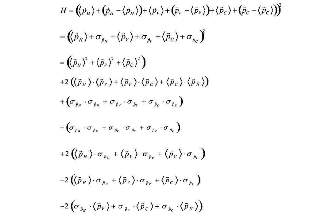
となる。さらに平均場近似の考え方を導入して、このモデル・ハミルトニアンに対して平均を取ると、ゆらぎの一次の項をもつ最後の3つの括弧でくくられた式は、ゆらぎ項の空間の広がり方向に関するベクトル成分が相殺し合い、ゆらぎ項の期待値は

となるので全て消滅する。従って、残るのは最初の4つの括弧でくくられた式のみとなる
。
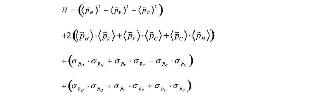
によって模式的に表す。ゆらぎ項についても、(明るさのゆらぎ幅)×(空間の広がり幅)の次元をもつ物理量を
によって模式的に表す。モデル・ハミルトニアンを展開すると
となる。さらに平均場近似の考え方を導入して、このモデル・ハミルトニアンに対して平均を取ると、ゆらぎの一次の項をもつ最後の3つの括弧でくくられた式は、ゆらぎ項の空間の広がり方向に関するベクトル成分が相殺し合い、ゆらぎ項の期待値は
となるので全て消滅する。従って、残るのは最初の4つの括弧でくくられた式のみとなる
。
平均項とゆらぎ項はそれぞれ明るさ方向と空間方向の積によって記述しているので、実際には平均項はベクトルによって、ゆらぎ項はテンソルによって記述することになる。詳細は実施形態の中で定義する。
このモデル・ハミルトニアンで記述した運動を、2次元平面の剛体の運動と対応づけて捉える。明るさ方向の強度値の分布が、剛体の運動に関する次元、すなわち単位時間当たりの変化率の次元を持つと位置づける。空間方向の分布は、剛体の静止した状態における形状因子を記述していて、距離に関する次元を持つと位置づける。
平均項が剛体の並進運動に関する記述を、ゆらぎ項が剛体の回転運動に関する記述をしていると捉える。剛体の運動に関する運動量、角運動量、エネルギーはそれぞれ次のような次元を持った形式で定義する。すなわち、運動量と角運動量は明るさ方向の強度の一次形式、エネルギーは明るさ方向の強度の2次形式となる。
運動量=(平均項)=(空間重心)×(明るさ平均)
角運動量=(広がり項)=(空間広がり)^2×(明るさ広がり)
エネルギー=(平均項の並進運動エネルギー)+(広がり項の回転運動エネルギー)
=(空間重心の距離)^2×(明るさ平均)^2+(空間広がり)^2×(明るさ広がり)^2
運動量=(平均項)=(空間重心)×(明るさ平均)
角運動量=(広がり項)=(空間広がり)^2×(明るさ広がり)
エネルギー=(平均項の並進運動エネルギー)+(広がり項の回転運動エネルギー)
=(空間重心の距離)^2×(明るさ平均)^2+(空間広がり)^2×(明るさ広がり)^2
モデル・ハミルトニアンを展開して平均場近似によって残った最初の2つの括弧でくくられた項が並進運動エネルギーを、最後の2つの括弧でくくられた項が回転運動エネルギーを表す。(空間広がり)^2は重心位置からの2次のモーメントの平均的広がりを表す慣性テンソルによって記述される。このように空間広がりを重心系を中心にした記述にすると、エネルギーの平均項とゆらぎ項の交差項の成分が消滅する。剛体運動に関する詳しい説明は文献H1においてなされている。また、H,V,C間でHV,VC,CHの組み合わせの交差項が出てくるのは、HVCが完全に独立な成分を記述していないことに由来して、その交差エネルギーを持つようにモデル・ハミルトニアンを構築したためである。
モデル・ハミルトニアンの展開によって導出された項の対応する具体的表式は、本実施形態の中で定義する。図25は構図の低次不変量の構築に関わる要素の関わりを示す図である。一次元分布で定義したときと同様にその延長で2次元分布のときも、運動量は平均項、角運動量は広がり項、あるいはゆらぎ項に対応している。
ここで、階調の一次元分布関数から導く特徴量と、構図の2次元分布関数から導く特徴量との間の関わりについて説明する。一次元分布関数で規定される部分系とは、明るさ因子の部分を通じて相互に相関をもって記述されている。すなわち、色の一次元分布の部分系と色の2次元分布の部分系は明るさ因子の部分に重なりを持った特徴量を導出する。エッジの一次元分布の部分系とエッジの2次元分布の部分系も明るさ因子の部分に重なりを持った特徴量を導出する。しかし、2次元分布から導いた特徴量には、空間因子に関する情報が新たに付け加わっており、一次元分布から導いた特徴量とは相互に独立な要素を記述していることになる。
[文献H1]ランダウ=リフシッツ理論物理学教程第1巻「力学」(増訂第3版、1973年)、第6章「剛体の運動」、第31節「角速度」、第32節「慣性テンソル」、及び第33節「剛体の角運動量」
<周波数記述による均等認識空間への写像>
これまで4つの主軸うち、色の一次元分布関数をヒルベルト空間に射影して周波数記述を行うときにはチェビシェフ関数を用い、エッジの一次元分布関数をヒルベルト空間に射影して周波数記述を行うときには球ベッセル関数を用いてきた。これは、分布関数の形状がとりうる拘束条件に適した形状認識を均等化する基底関数を選定しているためである。分布関数の形状を、基底関数の周波数分布を表す展開係数で記述することにより、均等認識空間へ写像していることになる。一般に、色の側面は超幾何関数に属する特殊関数によって記述し、エッジの側面は合流型超幾何関数に属する特殊関数によって記述するのがよいという原則を述べてきた。
これまで4つの主軸うち、色の一次元分布関数をヒルベルト空間に射影して周波数記述を行うときにはチェビシェフ関数を用い、エッジの一次元分布関数をヒルベルト空間に射影して周波数記述を行うときには球ベッセル関数を用いてきた。これは、分布関数の形状がとりうる拘束条件に適した形状認識を均等化する基底関数を選定しているためである。分布関数の形状を、基底関数の周波数分布を表す展開係数で記述することにより、均等認識空間へ写像していることになる。一般に、色の側面は超幾何関数に属する特殊関数によって記述し、エッジの側面は合流型超幾何関数に属する特殊関数によって記述するのがよいという原則を述べてきた。
残りの2つの主軸である色の2次元分布関数とエッジの2次元分布関数をヒルベルト空間表現するときの基底関数の選定にあたってもこの原則を当てはめる。実際には色の2次元分布関数の周波数表現に適した基底関数としてはルジャンドル陪関数を選ぶ。また、エッジの2次元分布関数の周波数表現に適した基底関数としてはフーリエ関数を選ぶ。以下にその選定理由を述べる。
1)色の2次元分布関数に対するルジャンドル陪関数の選定理由
ルジャンドル陪関数は超幾何関数の一種で、色の分布の記述に適している。ルジャンドル陪関数Pm l(x)は磁気量子数mと方位量子数lの2つの指数によって定義され、方位量子数lの異なる基底関数間では、基底関数の直交性は空間的な重みが均質な直交性を有する。磁気量子数m=0の最低次の方位量子数lがなす関数群P0 l(x)=Pl(x)はルジャンドル関数と呼ばれる。ルジャンドル陪関数の直交性の関係式と、ルジャンドル関数の基底関数の低周波側の具体式を挙げる。

ルジャンドル陪関数は超幾何関数の一種で、色の分布の記述に適している。ルジャンドル陪関数Pm l(x)は磁気量子数mと方位量子数lの2つの指数によって定義され、方位量子数lの異なる基底関数間では、基底関数の直交性は空間的な重みが均質な直交性を有する。磁気量子数m=0の最低次の方位量子数lがなす関数群P0 l(x)=Pl(x)はルジャンドル関数と呼ばれる。ルジャンドル陪関数の直交性の関係式と、ルジャンドル関数の基底関数の低周波側の具体式を挙げる。
ここで、図26はルジャンドル多項式におけるP2(x),P3(x,)P4(x),P5(x)のグラフである。ルジャンドル関数は、両端のx=-1とx=1に特異点を持っている。ルジャンドル関数は、この特異点の位置に電荷をおいたときの電気多重極子の分布に関する性質を記述するのに適した関数である。さらに、ルジャンドル関数の低周波側の第一波の関数はP1(x)=xでグラデーションを記述する。
これらの性質を画像に当てはめてみると、均質に分布している被写体像に対して、構図のフレーミングをするという切り込みを入れる。この切り込み点が画像として特異点となり、画像の構図的な側面から形状を認識するときにフレーミング効果として作用する。その特異点から見た形状分布に対して、多重極子の概念を含んだルジャンドル陪関数を用いて空間分布の周波数空間での高次元のモーメント解析を可能にする。画像としては、右端と左端、あるいは上端と下端に対して、地球でいえば北極と南極に相当するような特異点を持ちつつ、それにも関わらずその間の空間は一様に扱われる。これは空間をフレーミングして構図を切り取るという性質に合致する。更に、色の分布は青空のようにグラデーションが現れる性質を持っている。この点においてもルジャンドル関数は、その第1波がその基底関数を備えている点で、色の2次元分布関数を極めてコンパクトに周波数表現することに適した関数である。
なお、ルジャンドル陪関数の詳しい性質に関する説明は文献B3参照。
なお、ルジャンドル陪関数の詳しい性質に関する説明は文献B3参照。
[文献B3]ジョージアルフケン基礎物理数学第3巻「特殊関数と積分方程式」(第2版、1970;日本語訳 1978)、第2章「ルジャンドル関数」及び第3章「特殊関数」
2)エッジの2次元分布関数に対するフーリエ関数の選定理由
フーリエ関数は、特異点を3つ持つ超幾何関数や、特異点を2つ持つ合流型超幾何関数と異なり、特異点を持たない微分方程式の分類の関数に相当する。エッジの2次元分布関数は、正と負の値を持つエッジ面そのままの性質ではなく、それらを2乗した値の分布によって記述している。色面からエッジ面を検出した段階で、その画像は大部分で零に近い値を持つ。その上に2乗しているので、値の分布は極めて滑らかな波形形状となる性質がある。
フーリエ関数は、特異点を3つ持つ超幾何関数や、特異点を2つ持つ合流型超幾何関数と異なり、特異点を持たない微分方程式の分類の関数に相当する。エッジの2次元分布関数は、正と負の値を持つエッジ面そのままの性質ではなく、それらを2乗した値の分布によって記述している。色面からエッジ面を検出した段階で、その画像は大部分で零に近い値を持つ。その上に2乗しているので、値の分布は極めて滑らかな波形形状となる性質がある。
そうして得られた画像はコントラストの高いエッジ部分以外は大部分が真っ黒の画像で、仮に右端と左端の画像を接続して円筒形にしても、あるいは上端と下端の画像を接続して円筒形にしても、分布の違いによる異常な切れ込みは認識されずに、滑らかに接続する性質を備えた画像である。これは画像の両端で特異点を持たない無限に広がる波形で記述することが適していることを意味している。特異点を持たずに、両端での境界条件が値が零、ないし微分が零で接続する性質を持つフーリエ関数がこの画像の波形分布の特徴に極めて合致する。さらに、構図を扱うときに重要な性質となる空間を一様に扱う性質もフーリエ関数は備えている。一様な重み関数によるフーリエ関数の直交性の関係式を記しておく。

<周波数記述における部分系の間の相関>
4つの主軸の分布関数を周波数展開した各々の部分系の式を並べると、次のようになる。

4つの主軸の分布関数を周波数展開した各々の部分系の式を並べると、次のようになる。
主軸の分布関数に射影するという操作によって、画像の変数が変数分離され、色の一次元分布関数がスピン系の1つの独立変数に関する性質を、エッジの一次元分布関数が動径方向の1つの独立変数に関する性質を、色の2次元分布関数が天頂角方向の2つの独立変数に関する性質を、エッジの2次元分布関数が方位角方向の2つの独立変数に関する性質をそれぞれ記述していると位置づける。独立変数の軸としては6つあることになる。
エッジの一次元分布関数の球ベッセル展開を二重級数で行ったとき、次数lに関する直交性は、色の2次元分布を展開したルジャンドル陪関数の量子数lに関する基底関数の直交性が担う。従って、球ベッセル展開係数は、この部分系の中で閉じた状態で単独に、量子数nの根に関する直交性だけを満たすように決める。
色の2次元分布関数のルジャンドル陪関数展開を二重級数で行ったとき、次数mに関する直交性は、エッジの2次元分布を展開したフーリエ関数の量子数mに関する基底関数の直交性が担う。従って、ルジャンドル陪関数の展開係数は、この部分系の中で閉じた状態で単独に、量子数lに関する直交性だけを満たすように決める。
このように周波数記述においては、エッジの一次元分布関数の部分系と色の2次元分布関数の部分系との間で、更には色の2次元分布関数の部分系とエッジの2次元分布関数の部分系との間で、分布関数を同時記述することによって、基底関数の直交性が一方に反映されるという、部分系の間の相関が存在する。
このように周波数記述においては、エッジの一次元分布関数の部分系と色の2次元分布関数の部分系との間で、更には色の2次元分布関数の部分系とエッジの2次元分布関数の部分系との間で、分布関数を同時記述することによって、基底関数の直交性が一方に反映されるという、部分系の間の相関が存在する。
色面とエッジ面の2つの2次元分布関数を同時に展開すると、ルジャンドル陪関数とフーリエ関数の積が基底関数となるので、これらの基底関数はx方向とy方向のそれぞれについて球面調和関数を構成する。
<部分系の統計的独立性とエネルギー準位の分裂>
このように画像全体の分布関数は、部分系の分布関数の積で表されるので、それぞれの部分系は統計的独立性を保っている。それぞれの部分系である感性の1つの側面についてエネルギーに関する線形微分方程式を満たしていて、それからエネルギー固有値Enが導かれる。各々の部分系でそれぞれが満たす微分方程式からエネルギーの固有値が導かれてくる。そのとき全系のエネルギー固有値は、各部分系で導出されたエネルギー固有値の和で表される。従って、ある部分系では縮退していたエネルギー準位が、他の部分系の作用によって縮退した状態を解き、分裂したエネルギー準位を与えることになる。
このように画像全体の分布関数は、部分系の分布関数の積で表されるので、それぞれの部分系は統計的独立性を保っている。それぞれの部分系である感性の1つの側面についてエネルギーに関する線形微分方程式を満たしていて、それからエネルギー固有値Enが導かれる。各々の部分系でそれぞれが満たす微分方程式からエネルギーの固有値が導かれてくる。そのとき全系のエネルギー固有値は、各部分系で導出されたエネルギー固有値の和で表される。従って、ある部分系では縮退していたエネルギー準位が、他の部分系の作用によって縮退した状態を解き、分裂したエネルギー準位を与えることになる。
例えば、一次元系の色とエッジに関するエネルギー要素のみを用いて画像の特徴を記述していた場合、2次元の構図の分布に関して区別する能力を持たないが、構図に関連したエネルギー要素が2次元系で記述されると、そのエネルギー要素が今までの一次元系のエネルギー準位を分裂させ、区別することが可能になる。
軸反転した場合のエネルギー固有値を導く場合、部分系の統計的独立性からエネルギー固有値はそれぞれの部分系で独立に定まる。従って、軸反転性の性質については、各部分系単位で独立に軸反転した場合の性質を調べて、エネルギー要素を求めればよい。なお、軸反転性の性質を調べるのは、偶関数と奇関数からなる基底関数を用いて周波数空間記述する部分系に対してだけの特有の事項である。実空間記述では、このような操作は存在しない。
<構図の高次不変量>
まず、エネルギー要素Enについて、周波数空間(k空間)におけるエネルギー分散関係と既約表現の観点から定義を行っていく。周波数空間に投影された2次元展開係数cijを何らかの方法で一次元化して配列ciとし、α面の展開係数とβ面の展開係数との積から対称積と反対称積の2次形式エネルギーを定義する。ここでは話を分かりやすくするため対称積の場合だけを扱う。

ここに、2次形式和はα面とβ面の2次元面の全ての要素の積の和をとる。
すなわち、2次元係数面でどの点を始点としてどの方向に一方のα面の並べ方を選び、もう一方のβ面の並べ方もどの点を始点としてどの方向に並べたものと組み合わせるか、という課題がある。そのときの並べ方として、α面とβ面の組み合わせの積によって記述される2次元係数面の係数分布の性質を、最も効率よくコンパクトに表現する既約表現は存在しないか、という問題提起である。これを固体物理学の周期的な結晶構造がなすエネルギーバンドの性質を記述するときの方法になぞらえて構築する。
まず、エネルギー要素Enについて、周波数空間(k空間)におけるエネルギー分散関係と既約表現の観点から定義を行っていく。周波数空間に投影された2次元展開係数cijを何らかの方法で一次元化して配列ciとし、α面の展開係数とβ面の展開係数との積から対称積と反対称積の2次形式エネルギーを定義する。ここでは話を分かりやすくするため対称積の場合だけを扱う。
ここに、2次形式和はα面とβ面の2次元面の全ての要素の積の和をとる。
すなわち、2次元係数面でどの点を始点としてどの方向に一方のα面の並べ方を選び、もう一方のβ面の並べ方もどの点を始点としてどの方向に並べたものと組み合わせるか、という課題がある。そのときの並べ方として、α面とβ面の組み合わせの積によって記述される2次元係数面の係数分布の性質を、最も効率よくコンパクトに表現する既約表現は存在しないか、という問題提起である。これを固体物理学の周期的な結晶構造がなすエネルギーバンドの性質を記述するときの方法になぞらえて構築する。
周波数展開された2次元展開係数は、波動ベクトルのkx,kyで表された2次元のk空間を張っていると考えることができる。

x軸方向の最も高周波の成分が、x軸方向の最も低周波の成分と接続していると定義する。y方向についても同様に、y軸方向の最も高周波の成分が、y軸方向の最も低周波の成分と接続していると定義する。すなわち、超高周波は波の振動が多すぎて全体としては超低周波と同等に認識するという考え方である。これは一次元分布関数の基底関数から拡張シュプールによってエネルギー要素を定義するときにも導入している考え方である。
x軸方向の最も高周波の成分が、x軸方向の最も低周波の成分と接続していると定義する。y方向についても同様に、y軸方向の最も高周波の成分が、y軸方向の最も低周波の成分と接続していると定義する。すなわち、超高周波は波の振動が多すぎて全体としては超低周波と同等に認識するという考え方である。これは一次元分布関数の基底関数から拡張シュプールによってエネルギー要素を定義するときにも導入している考え方である。
そうすると、c0,n-1の次の高周波成分はc00となり、この2つの成分は量子数が1つだけずれたほぼ等価点と考えることができる。n×n個の展開係数で表されているとき、これらの展開係数の接続性に関する性質は、k空間で正方形のブリルアンゾーンを張っていることと同じになる。c00はk空間では(kx,ky)=(0,0)に対応し、c0,n-1はk空間では(kx,ky)=(2π/a,0)に対応し、cn-1,0はk空間では(kx,ky)=(0,2π/a)に対応し、cn-1,n-1はk空間では(2π/a,2π/a)の点に対応する。
最高周波の次に低周波を接続するという定義は、高周波成分が低周波成分として折り返す性質と同等で、一次元のk空間の場合は、kx=0~2π/aの周波数帯域を、kx=0~π/aの区間をそのまま残し、kx=π/a~2π/aの区間を左側にそのまま-2π/a分ずらしてkx=0=2π/aの等価点として接続し、kx=-π/a~π/aの範囲の区間で表現し直すことができる。これはブリルアンゾーンの性質そのものである。2次元のブリルアンゾーンとして、kx=0~2π/a,ky=0~2π/aで張る空間と、正の半分の区間を負の区間で表現して、kx=-π/a~π/a,ky=-π/a~π/aで張る空間と等価である。すなわち、n×n個の展開係数は、固体物理学における正方格子のブリルアンゾーンと同じ性質を持つ。
固体物理学において結晶構造のエネルギーバンドの性質、すなわちエネルギー分散関係E(k)を調べるとき、全てのk空間上の点の性質を調べなくても、ある特別な点と線上の性質だけを調べれば十分であることが空間群の既約表現という群論の考え方によって示される(文献H1、H2参照)。
文献H2によると正方格子のブリルアンゾーンの中には6個の特別の型の点もしくは直線が存在する。すなわち、ブリルアンゾーンが|kx|≦π/a、|ky|≦π/aの範囲で表されているとき、(kx,ky)=(0,0)のΓ点、(kx,ky)=(π/a,π/a)のM点、(kx,ky)=(π/a,0)のX点、Γ点とM点を結ぶΣ線、Γ点とX点を結ぶΔ線、M点とX点を結ぶZ線がそれに相当する。
これと同様の演繹から2次元係数面上で一次元化するとき、

をα面の係数の並べ替えの始点の位置と方向を規定するベクトルと定義する。このように並べ替えられた二つの係数からi番目の展開係数とj番目の展開係数を交換して互いにj=i+nの関係を保ったもの同士の間で対称積の和をとり、対称積の和が作るエネルギー分散関係

を調べたい。反対称積の和についても同様である。
これと同様の演繹から2次元係数面上で一次元化するとき、
をα面の係数の並べ替えの始点の位置と方向を規定するベクトルと定義する。このように並べ替えられた二つの係数からi番目の展開係数とj番目の展開係数を交換して互いにj=i+nの関係を保ったもの同士の間で対称積の和をとり、対称積の和が作るエネルギー分散関係
を調べたい。反対称積の和についても同様である。
無数にある並進ベクトルの選び方

の組み合わせでできる

が作る2次形式のエネルギーの性質を表すための既約表現は、正方格子のブリルアンゾーンが持つ空間群の既約表現と一致すると仮定する。その並べ替えの方法は、図27に示す6通りとその反対向きの負の方向を含めた12通りとなる。すなわち、正方格子のブリルアンゾーンの特別の点から特別の直線がのびる方向に向かって並び替える。
の組み合わせでできる
が作る2次形式のエネルギーの性質を表すための既約表現は、正方格子のブリルアンゾーンが持つ空間群の既約表現と一致すると仮定する。その並べ替えの方法は、図27に示す6通りとその反対向きの負の方向を含めた12通りとなる。すなわち、正方格子のブリルアンゾーンの特別の点から特別の直線がのびる方向に向かって並び替える。
更に、2つの係数面から対称積と反対称積を作るときのiとjを交換するときのずらし量n=i-jは特別の直線上の点だけずらした性質を調べればよい。n×n個の展開係数があるときは、n×n個全てずらさなくてもn個分だけずらしたエネルギー分散関係を、各々の方向組み合わせ、すなわち、12×12通りの組み合わせのそれぞれについて、α面側の始点は固定して、β面側の始点を特別の点から徐々に特別の線上に沿ってずらしていったときの、対称積と反対称積のエネルギー分散関係を求める。
図28はエネルギー分散関係の概念的な様子を示す図である。図29はk空間上での特別な点と線上でのエネルギーの性質を調べている様子を示す図であって12方向の並び替えとそこから特別の直線上に沿って、i-jの量子数をずらしていったときのk空間上で調べている位置の様子を示している。ここで12方向の並び替えを表す記号として、±v,±h,±d,±d',+h/2±v,+v/2±hを用いる。図30は2次元展開係数と運動量、角運動量、エネルギーの関係を示す図である。
このように展開係数の2次形式和をとったエネルギー分散関係は、展開係数そのものを運動量と考えると、位相空間上での同一の軌道をとる同一感性を与える画像分布の和集合を記述している。すなわち、空などの背景は横方向にのっぺりとしたグラデーション地帯が現れやすく、山々には横方向にテキスチャ帯が現れやすい。このような周波数に関する性質を個別の周波数分布が一致していなくても全体的な周波数の分布に関する情報が一致している包括的な指標として、感性の曖昧性を記述している。
それと共にk空間で1/2の周波数を始点とした並び替えと最低次周波数、あるいは最高次周波数を始点とした並び替えとの組み合わせの性質を調べているので、縦方向や横方向、斜め方向との間でスケールが半分になっても似たような周波数構造を持つパターンが存在しているか否かの性質をも表している。すなわち、2次元形状分布の中の構造に関して、フラクタル性の存在を評価している指標でもある。
並び替え方の詳細についてもう一度説明する。以下の説明では左端を一行一列目、右端をn行n列目とする。
+v方向の並び替えは、一列目を上から順にn個分を取り出し、次に2列目を上から順にn個分を取り出して、最後まで繰り返す。-v方向の並び替えは、n列目を下から順にn個分を取り出し、次にn-1列目を下から順にn個分取り出して、最後まで繰り返す。
+v方向の並び替えは、一列目を上から順にn個分を取り出し、次に2列目を上から順にn個分を取り出して、最後まで繰り返す。-v方向の並び替えは、n列目を下から順にn個分を取り出し、次にn-1列目を下から順にn個分取り出して、最後まで繰り返す。
+h方向の並び替えは、一行目を左から順にn個分を取り出し、次に2行目を左から順にn個分を取り出して、最後まで繰り返す。-h方向の並び替えは、n行目を右から順にn個分を取り出し、次にn-1行目を右から順にn個分取り出して、最後まで繰り返す。
+h/2+v方向の並び替えは、n/2列目を上から順にn個分を取り出し、次にn/2+1列目を上から順にn個分を取り出し、n列目が終わった次は1列目を取り出しに行き、n/2-1列目まで繰り返す。+h/2-v方向の並び替えは、n/2-1列目を下から順にn個分を取り出し、次にn/2-2列目を下から順にn個分取り出して、1列目が終わった次はn列目を取り出しに行き、n/2列目まで繰り返す。
+h/2+v方向の並び替えは、n/2列目を上から順にn個分を取り出し、次にn/2+1列目を上から順にn個分を取り出し、n列目が終わった次は1列目を取り出しに行き、n/2-1列目まで繰り返す。+h/2-v方向の並び替えは、n/2-1列目を下から順にn個分を取り出し、次にn/2-2列目を下から順にn個分取り出して、1列目が終わった次はn列目を取り出しに行き、n/2列目まで繰り返す。
+v/2+h方向の並び替えは、n/2行目を左から順にn個分を取り出し、次にn/2+1行目を左から順にn個分を取り出し、n行目が終わった次は1行目を取り出しに行き、n/2-1行目まで繰り返す。+h/2-v方向の並び替えは、n/2-1行目を右から順にn個分を取り出し、次にn/2-2行目を右から順にn個分取り出して、1行目が終わった次はn行目を取り出しに行き、n/2行目まで繰り返す。
+d方向の並び替えは、一行一列目を始点に右下方向に順にn個分を取り出し、次に2行一列目を始点に右下方向に順にn個分を取り出し、n行1列目を始点にn個分を取り出すまで繰り返す。このとき、定義域から正の方向にはみ出した行番号はn個分引き算したところを対応点とする。-d方向の並び替えは、n-1行n列目を始点に左上方向に順にn個分を取り出し、次にn-2行n列目を始点に左上方向に順にn個分を取り出し、1行n列目を始点にn個分を取り出した後、n行n列目を始点にn個分を取り出す。このとき、定義域から負の方向にはみ出した行番号はn個分足し算したところを対応点とする。
+d'方向の並び替えは、一行n列目を始点に左下方向に順にn個分を取り出し、次に2行n列目を始点に左下方向に順にn個分を取り出し、n行n列目を始点にn個分を取り出すまで繰り返す。このとき、定義域から正の方向にはみ出した行番号はn個分引き算したところを対応点とする。-d'方向の並び替えは、n-1行1列目を始点に右上方向に順にn個分を取り出し、次にn-2行1列目を始点に右上方向に順にn個分を取り出し、1行1列目を始点にn個分を取り出した後、n行1列目を始点にn個分を取り出す。このとき、定義域から負の方向にはみ出した行番号はn個分足し算したところを対応点とする。
次に角運動量に関して定義する。物体の運動の記述において、角運動量が運動の恒量になりうるのは、球対称なポテンシャルで表される中心力場に対してのみである(文献H4参照)。これを画像の分布に当てはめてみると、中心対称な形状の特徴だけが、空間の等方性に関して保存量となる。2次元展開係数の中で中心対称な性質を示すのは対角成分だけである。
古典的な角運動量の定義に従って、展開係数を運動量と捉え、座標を展開係数の量子数を表すヒルベルト空間座標に対応づけると、角運動量は対角成分を量子数倍した和で記述できる。
古典的な角運動量の定義に従って、展開係数を運動量と捉え、座標を展開係数の量子数を表すヒルベルト空間座標に対応づけると、角運動量は対角成分を量子数倍した和で記述できる。
角運動量が意味のある運動の恒量として記述されうる画像の例としては、各国の国旗のような中心に丸があるような画像群や中心に主要被写体を配置した撮影構図の画像がある。ある印象を発する形容詞にとって、中心対称性が重要視される場合には、この特徴量が有効な作用を及ぼす。それ以外の場合は中心対称性を備えない画像との統計平均によってこの特徴量は消滅する。
[文献H2]キッテル「固体の量子論」(1963)、第10章「ブリルアン・ゾーンと結晶対称性」
[文献H3]ランダウ=リフシッツ理論物理学教程第5巻「統計物理学第一部」(第3版、1976年)、第13章「結晶の対称性」、第134節「空間群の既約表現」
[文献H4]シッフ「量子力学」(第3版、1970)、第4章「離散的な固有値:束縛状態」、第14節「三次元の球対称なポテンシャル」
[文献H3]ランダウ=リフシッツ理論物理学教程第5巻「統計物理学第一部」(第3版、1976年)、第13章「結晶の対称性」、第134節「空間群の既約表現」
[文献H4]シッフ「量子力学」(第3版、1970)、第4章「離散的な固有値:束縛状態」、第14節「三次元の球対称なポテンシャル」
<高次不変量の軸反転性に対する不変性>
上述のように基底関数を用いて周波数空間に投影した展開係数から作成した2次形式のエネルギーなどの高次不変量は、(α)(x,y)、(β)(x,y)の元の2次元分布面そのものの展開係数で構成される。2次元分布の構図系においても、一次元分布の周波数記述の時に導入したのと同じようにして、軸反転した場合も独立なエネルギー要素を生み出すので、これらも新たな特徴量とする。
上述のように基底関数を用いて周波数空間に投影した展開係数から作成した2次形式のエネルギーなどの高次不変量は、(α)(x,y)、(β)(x,y)の元の2次元分布面そのものの展開係数で構成される。2次元分布の構図系においても、一次元分布の周波数記述の時に導入したのと同じようにして、軸反転した場合も独立なエネルギー要素を生み出すので、これらも新たな特徴量とする。
軸反転の仕方として、α面とβ面のそれぞれで4通りずつ存在するので、独立なエネルギー要素は、軸反転性を考慮しない場合の4×4倍の要素が生み出される。
(α)(x,y)、
(α)(x,-y)=(α')(x,y)、
(α)(-x,y)=(α")(x,y)、
(α)(-x,-y)=(α"')(x,y)、
(β)(x,y)、
(β)(x,-y)=(β')(x,y)、
(β)(-x,y)=(β")(x,y)、
(β)(-x,-y)=(β"')(x,y)
(α)(x,y)、
(α)(x,-y)=(α')(x,y)、
(α)(-x,y)=(α")(x,y)、
(α)(-x,-y)=(α"')(x,y)、
(β)(x,y)、
(β)(x,-y)=(β')(x,y)、
(β)(-x,y)=(β")(x,y)、
(β)(-x,-y)=(β"')(x,y)
これらのエネルギー要素を全て固有値として持つハミルトニアンによって、部分系が記述されているならば、同一の感性を表す画像群が、ハミルトニアンの軸反転性に対する不変性をもって記述されていることになる。すなわち、軸反転すると奇関数の展開係数として、異なる係数分布が生じるので、たまたまある画像と軸反転した画像が同じ係数分布をしていたとしても、軸反転前同士のエネルギー要素と、軸反転後同士のエネルギー要素の振る舞いの違いをみるので、これらの画像は形容詞の印象として別物に属すると区別することができる。
軸反転した色面から作られるエネルギー分散関係は、軸反転なしの元の状態のエネルギー分散関係で記述されていない特別の点と特別の点の間の分散関係を、両端の特別の点を共有しながら埋めていくような記述効果がある。すなわち、両端の特別の点では状態は縮退している。
なお、ここで第7の実施形態まで行ってきた説明に対して、共通して補足説明を行う。
<状態数の勘定方法>
状態数の勘定方法について、実空間記述を行うときの低次不変量のエネルギーを作成するときにモデル・ハミルトニアンを導入した。そのモデル・ハミルトニアンを展開すると異なる色面の(α)面と(β)面の積からなる項は、同じ色面の(α)面と(α)面の積からなる項の2倍因子を伴う。これは2つの組み合わせ状態を選ぶとき、(α)面と(β)面の積が(α)(β)と(β)(α)の等価な2つの選び方が存在していることに伴う。また、同様にして、平均項とゆらぎ項との積には2倍因子を伴っている。これらは、本来状態が2倍存在するものとして、エネルギー要素の値を計算したとき、同じエネルギー要素を2度定義するか、エネルギー要素の値を2倍して定義するかのどちらかを採用して、状態の縮退数分を加味した補正を行っておくのがより適切である。
(α)面と(β)面の積で定義されるエネルギー要素を2倍にするのは、周波数空間記述を行う高次系不変量に対しても当てはまる。
<形容詞モデル分布の構築法>
これまで画像から受ける印象を心理的に線形なスケールで5段階で評価したものを、形容詞モデル分布として構築するとき、5段階のものを1倍、4段階のものを0.8倍、3段階のものを0.6倍、2段階のものを0.4倍、1段階のものを0.2倍という重みを掛けてきた。この重みの付け方の他に、例えば、5段階評価を自然対数の値と解釈して、5段階評価の画像のそれぞれに5段階のものから順に、exp(0)倍=1、exp(-1)倍、exp(-2)倍、exp(-3)倍、exp(-4)倍の重みを付けて形容詞モデル分布を構築するようにしてもよい。
これまで画像から受ける印象を心理的に線形なスケールで5段階で評価したものを、形容詞モデル分布として構築するとき、5段階のものを1倍、4段階のものを0.8倍、3段階のものを0.6倍、2段階のものを0.4倍、1段階のものを0.2倍という重みを掛けてきた。この重みの付け方の他に、例えば、5段階評価を自然対数の値と解釈して、5段階評価の画像のそれぞれに5段階のものから順に、exp(0)倍=1、exp(-1)倍、exp(-2)倍、exp(-3)倍、exp(-4)倍の重みを付けて形容詞モデル分布を構築するようにしてもよい。
[第8の実施形態]
第6の実施形態では、色とエッジの一次元分布関数から作られる実空間表現と周波数空間表現の4部分系までを「感性の線形モデル」によって記述したが、第8の実施形態ではこれらの上に、更に構図に関する色とエッジの2次元部分布関数から作られる実空間表現と周波数空間表現の4部分系を追加した系を記述する。なお、ここでも、これまでテキスチャと呼んでいた部分系は、これ以降ではエッジと呼び直すことにする。
第6の実施形態では、色とエッジの一次元分布関数から作られる実空間表現と周波数空間表現の4部分系までを「感性の線形モデル」によって記述したが、第8の実施形態ではこれらの上に、更に構図に関する色とエッジの2次元部分布関数から作られる実空間表現と周波数空間表現の4部分系を追加した系を記述する。なお、ここでも、これまでテキスチャと呼んでいた部分系は、これ以降ではエッジと呼び直すことにする。
第6の実施形態と異なる部分だけ記載する。第6の実施形態では「一次元」と付いていなかったタイトルには、本実施形態では付いているものが対応する。「二次元」と付いているタイトルの部分が新たに付け加える部分である。
1.マンセルHVC色空間への変換
2.HVC面のエッジ画像の作成
3.一次元色分布の低次不変量の作成
4.一次元色分布の高次不変量の作成
5.一次元エッジ分布の低次不変量の作成
6.一次元エッジ分布の高次不変量の作成
1.マンセルHVC色空間への変換
2.HVC面のエッジ画像の作成
3.一次元色分布の低次不変量の作成
4.一次元色分布の高次不変量の作成
5.一次元エッジ分布の低次不変量の作成
6.一次元エッジ分布の高次不変量の作成
spdf展開する場合について説明する。
6-0.低次系の分布関数のヒルベルト空間表現
6-0-1.変数変換
第3の実施形態の手順4-1と同じ。
6-0.低次系の分布関数のヒルベルト空間表現
6-0-1.変数変換
第3の実施形態の手順4-1と同じ。
6-0-2.球ベッセル関数による級数展開
H,V,C各色面の一次元分布関数をN個の根による係数と4個の次数からなる球ベッセル関数で2重級数展開して等価表現する。

H,V,C各色面の一次元分布関数をN個の根による係数と4個の次数からなる球ベッセル関数で2重級数展開して等価表現する。
まず、方位量子数lに関しては、l=0~3の中の偶関数と奇関数の2つの量子数だけを用い、主量子数nに関する根による二重級数展開によって等価表現を行なう。方位量子数4つの中からの2つを選ぶ組み合わせについては、偶関数と奇関数を必ず選ぶ条件を満たせば、任意性がある。例えばl=0,1の組み合わせとl=2,3の組み合わせもどちらも一次元分布関数を等価表現しうる。そのときの係数は以下の展開で規定される。

展開係数cl
nは、基底関数の直交性を利用して以下の式で求められる。なおαlnは前記の[数50]で示した式によって与えられる。

l=0~3までの二重級数展開するときの方位量子数間の重みblは均等配分の1とする。方位量子数lの間の直交性は、統合エッジ画像のヒストグラムの一次元分布関数

と色面の2次元分布関数

を2つの分布関数の積によって同時展開したとき、色面の2次元分布関数のルジャンドル陪関数の直交性によって保証される。
と色面の2次元分布関数
を2つの分布関数の積によって同時展開したとき、色面の2次元分布関数のルジャンドル陪関数の直交性によって保証される。
この部分系の不変量の計算に使う展開係数clnは、偶関数と奇関数を1つずつ用いた二重級数で求まった展開係数cl
nと等しくなる。以後では、cl
nをclnとして扱う。
6-1.高次系の分布関数の作成
第5の実施形態の6-1で示した手順と同様である。
6-2.エントロピーの計算
第5の実施形態の6-2で示した手順と同様である。
6-3.運動量の要素pnの計算
第5の実施形態の6-3で示した手順と同様である。
第5の実施形態の6-1で示した手順と同様である。
6-2.エントロピーの計算
第5の実施形態の6-2で示した手順と同様である。
6-3.運動量の要素pnの計算
第5の実施形態の6-3で示した手順と同様である。
6-4.角運動量の要素Mnの計算
角運動量の要素Mnとしては以下のものが挙げられる。

軸反転した場合の独立成分

角運動量の要素の数は3面分あるから2×3=6個である。
角運動量の要素Mnとしては以下のものが挙げられる。
軸反転した場合の独立成分
角運動量の要素の数は3面分あるから2×3=6個である。
6-5.エネルギーの要素Enの計算
spdf展開したときの実際に用いる規格化を含めたエネルギーの要素を以下に示す。

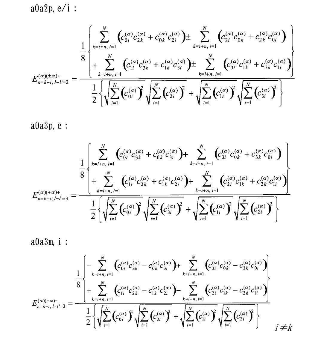
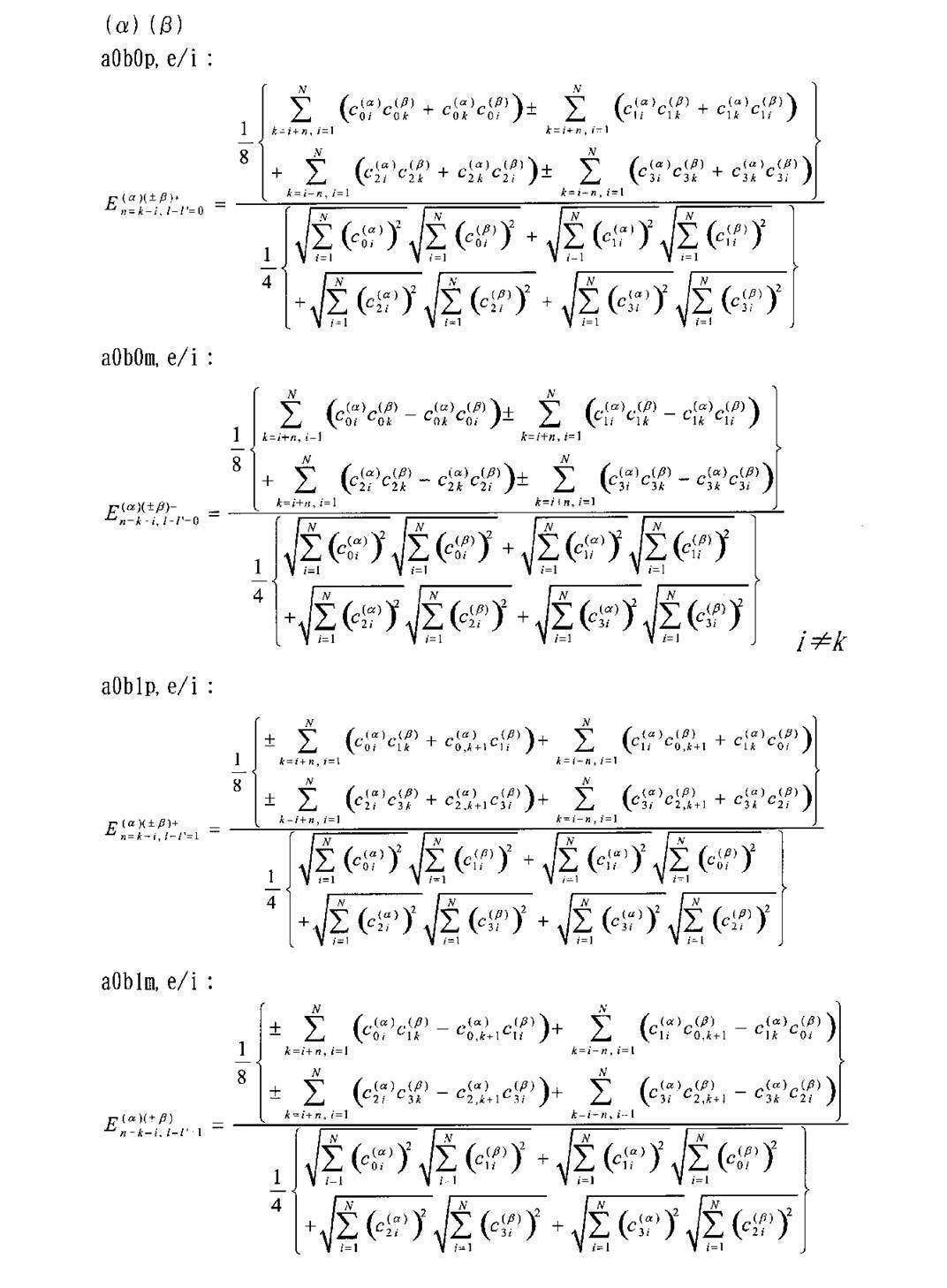
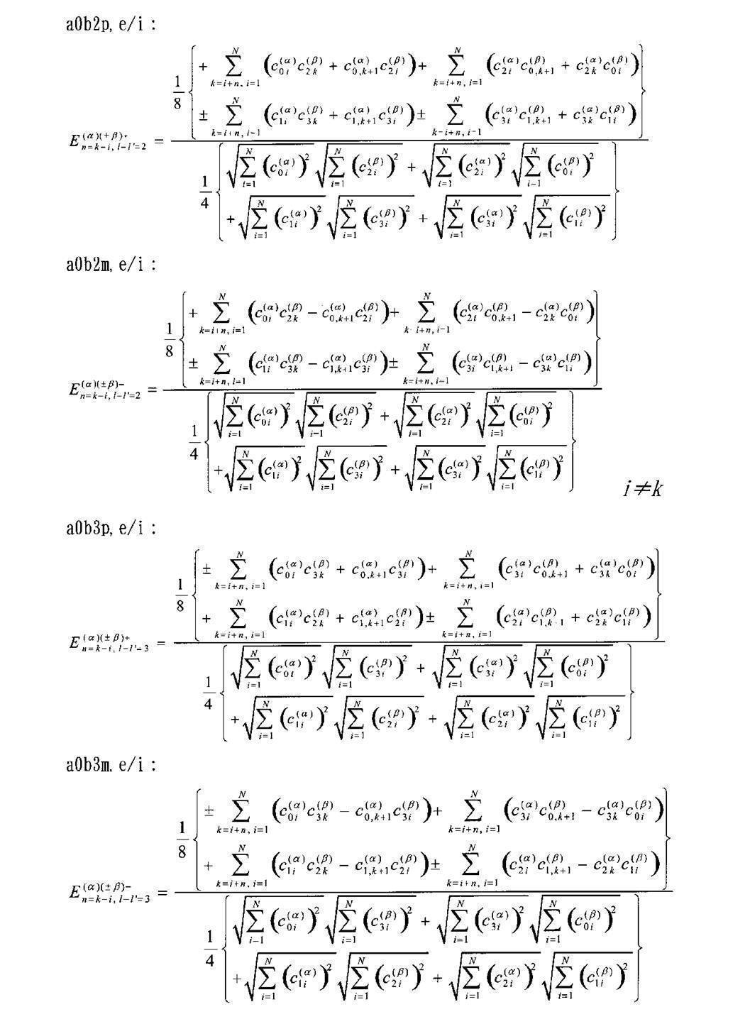
spdf展開したときの実際に用いる規格化を含めたエネルギーの要素を以下に示す。
なお、上述のsp展開からspdf展開へ拡張したのと同様の手続きをとれば、更に二重級数における角運動量量子数の展開次数を上げたときも同様に定義できる。角運動量量子数l=0,1,...,15までの展開を行ったときのα面とβ面の部分行列(l,l')の組み合わせ方だけを以下に示しておく。
00型 (l,l')=(0,0)+(1,1)+(2,2)+(3,3)+(4,4)+(5,5)+(6,6)+(7,7)
+(8,8)+(9,9)+(10,10)+(11,11)+(12,12)+(13,13)+(14,14)+(15,15)
01型 (l,l')=(0,1)+(1,0)+(2,3)+(3,2)+(4,5)+(5,4)+(6,7)+(7,6)
+(8,9)+(9,8)+(10,11)+(11,10)+(12,13)+(13,12)+(14,15)+(15,14)
02型 (l,l')=(0,2)+(2,0)+(1,3)+(3,1)+(4,6)+(6,4)+(5,7)+(7,5)
+(8,10)+(10,8)+(9,11)+(11,9)+(12,14)+(14,12)+(13,15)+(15,13)
03型 (l,l')=(0,3)+(3,0)+(2,5)+(5,2)+(4,7)+(7,4)+(6,9)+(9,6)
+(8,11)+(11,8)+(10,13)+(13,10)+(12,15)+(15,12)+(14,1)+(1,14)
04型 (l,l')=(0,4)+(4,0)+(1,5)+(5,1)+(2,6)+(6,2)+(3,7)+(7,3)
+(8,12)+(12,8)+(9,13)+(13,9)+(10,14)+(14,10)+(11,15)+(15,11)
05型 (l,l')=(0,5)+(5,0)+(2,7)+(7,2)+(4,9)+(9,4)+(6,11)+(11,6)
+(8,13)+(13,8)+(10,15)+(15,10)+(12,1)+(1,12)+(14,3)+(3,14)
06型 (l,l')=(0,6)+(6,0)+(1,7)+(7,1)+(4,10)+(10,4)+(5,11)+(11,5)
+(8,14)+(14,8)+(9,15)+(15,9)+(12,2)+(2,12)+(13,3)+(3,13)
07型 (l,l')=(0,7)+(7,0)+(2,9)+(9,2)+(4,11)+(11,4)+(6,13)+(13,6)
+(8,15)+(15,8)+(10,1)+(1,10)+(12,3)+(3,12)+(14,5)+(5,14)
08型 (l,l')=(0,8)+(8,0)+(1,9)+(9,1)+(2,10)+(10,2)+(3,11)+(11,3)
+(4,12)+(12,4)+(5,13)+(13,5)+(6,14)+(14,6)+(7,15)+(15,7)
09型 (l,l')=(0,9)+(9,0)+(2,11)+(11,2)+(4,13)+(13,4)+(6,15)+(15,6)
+(8,1)+(1,8)+(10,3)+(3,10)+(12,5)+(5,12)+(14,7)+(7,14)
10型 (l,l')=(0,10)+(10,0)+(1,11)+(11,1)+(4,14)+(14,4)+(5,15)+(15,5)
+(8,2)+(2,8)+(9,3)+(3,9)+(12,6)+(6,12)+(13,7)+(7,13)
11型 (l,l')=(0,11)+(11,0)+(2,13)+(13,2)+(4,15)+(15,4)+(6,1)+(1,6)
+(8,3)+(3,8)+(10,5)+(5,10)+(12,7)+(7,12)+(14,9)+(9,14)
12型 (l,l')=(0,12)+(12,0)+(1,13)+(13,1)+(2,14)+(14,2)+(3,15)+(15,3)
+(4,8)+(8,4)+(5,9)+(9,5)+(6,10)+(10,6)+(7,11)+(11,7)
13型 (l,l')=(0,13)+(13,0)+(2,15)+(15,2)+(4,1)+(1,4)+(6,3)+(3,6)
+(8,5)+(5,8)+(10,7)+(7,10)+(12,9)+(9,12)+(14,11)+(11,14)
14型 (l,l')=(0,14)+(14,0)+(1,15)+(15,1)+(4,2)+(2,4)+(5,3)+(3,5)
+(8,6)+(6,8)+(9,7)+(7,9)+(12,10)+(10,12)+(13,11)+(11,13)
15型 (l,l')=(0,15)+(15,0)+(2,1)+(1,2)+(4,3)+(3,4)+(6,5)+(5,6)
+(8,7)+(7,8)+(10,9)+(9,10)+(12,11)+(11,12)+(14,13)+(13,14)
6-6.部分系の温度の計算
第6の実施形態の4-6で示した手順と同様である。
6-7.部分系の自由エネルギーの計算
第6の実施形態の4-7で示した手順と同様である。
第6の実施形態の4-6で示した手順と同様である。
6-7.部分系の自由エネルギーの計算
第6の実施形態の4-7で示した手順と同様である。
7.二次元色分布の低次不変量の作成
この部分系を区別するための記号として不変量に対してHoという記号を用いる場合がある。
7-1.低次系の分布関数の作成
第2の実施形態でウェーブレット変換を用いた多重解像度変換することによって、LL成分の連なりによって元の画像の低周波成分、すなわち、縮小画像に相当する画像が生成されている。多重解像度の段数は、最低解像度が40×30~80×60程度の画像範囲に入る程度まで分解しているので、最低解像度から3段程度高解像度に位置する320×240画素程度のLL成分を縮小画像の色面として取り出す。HVC各色面について取り出し、それぞれの信号面をH(x,y),V(x,y),C(x,y)と表す。ここで用いている色相面はニュートラルの分離を行っていない色面である。すなわち、全て色相環の値のみで記述されている画像である。
これらの色面の画像の分布を剛体面と捉えて、剛体が持つ空間的な因子に関する性質を調べるための2次元分布関数を以下のように定義する。
剛体の分布関数
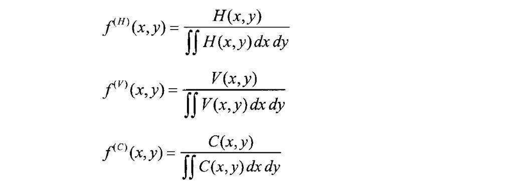
剛体の分布関数
2次元系では上記の3つの分布関数が基本であるが、後の色面間で交差定義する慣性テンソルの計算をするために、例外的に色面間の交差する分布関数を定義する。
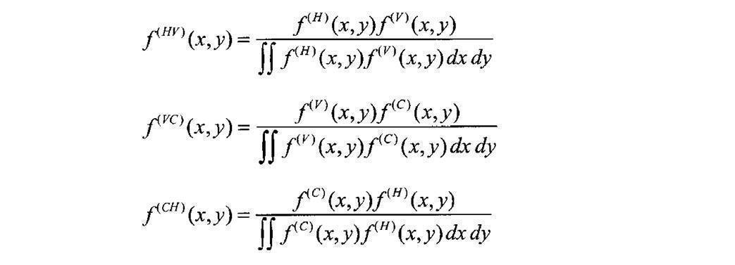
7-2.エントロピーの計算
色面の分布関数f(x,y)からエントロピーSを計算する。分布関数の値が0のところは、その状態をとらないという意味で、積分区間から排除するものとする。分布関数の色面を(α)で区別して表すと、H,V,C面の各々の分布関数からエントロピーが算出され、それらの和が2次元色分布の低次系に射影された部分系のエントロピーを表す。

この値をSHoとする。
色面の分布関数f(x,y)からエントロピーSを計算する。分布関数の値が0のところは、その状態をとらないという意味で、積分区間から排除するものとする。分布関数の色面を(α)で区別して表すと、H,V,C面の各々の分布関数からエントロピーが算出され、それらの和が2次元色分布の低次系に射影された部分系のエントロピーを表す。
この値をSHoとする。
7-3.運動量の要素pnの計算
まず、剛体面の空間的な形状因子に関する性質を調べる。すなわち、分布関数を用いて各色面の一次モーメントの平均である重心位置と、2次モーメントの平均を表す慣性テンソルを求める。重心は空間的な平均を表し、慣性テンソルは空間的な広がりを表す指標である。なお、H面の場合を例に示すが、V面、C面についても全く同様である。

まず、剛体面の空間的な形状因子に関する性質を調べる。すなわち、分布関数を用いて各色面の一次モーメントの平均である重心位置と、2次モーメントの平均を表す慣性テンソルを求める。重心は空間的な平均を表し、慣性テンソルは空間的な広がりを表す指標である。なお、H面の場合を例に示すが、V面、C面についても全く同様である。
2つの色面間で交差する分布に関しても同様に、重心位置と慣性テンソルを求める。なお、HV間の場合の例を示すが、VC間、CH間についても全く同様である。
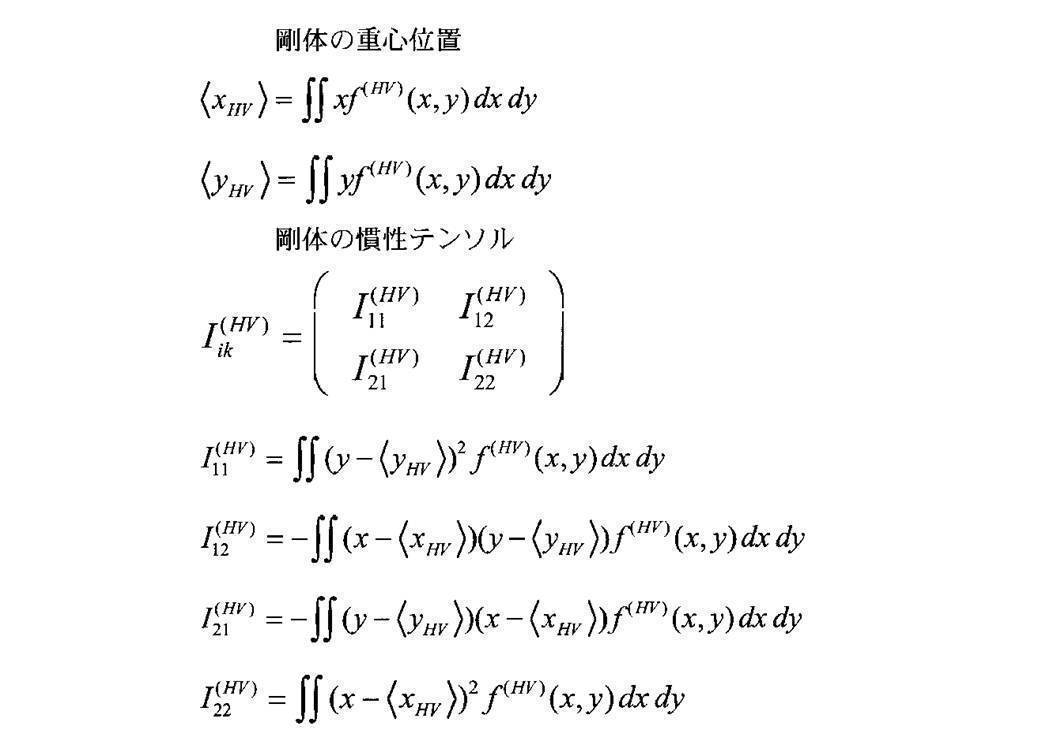
なお、座標軸と座標スケールの取り方は任意であるが、画像の中心を原点にとり、縦×横の長辺側の長さを1となるように定義すれば、重心位置や慣性テンソルの値は全て[-1,1]に収まるので便利である。
次に、速度、あるいは運動量の次元を持つ画像の明るさ因子に関する性質を調べる。画像の明るさレベルの平均的変化をx軸側に射影した場合と、y軸側に射影した場合の2つの成分に分けて調べる。なお、ここでもH面の場合の例だけを示す。
y軸方向に平均操作をしてx軸に射影した画像をH(x)、x軸方向に平均操作をしてy軸に射影した画像をH(y)とする。さらに色面全体の平均値<H>も算出する。

y軸方向に平均操作をしてx軸に射影した画像をH(x)、x軸方向に平均操作をしてy軸に射影した画像をH(y)とする。さらに色面全体の平均値<H>も算出する。
明るさの因子に関して画像全体の平均値とx,yへの射影軸におけるゆらぎ幅を求める。空間因子として計算した剛体系に対して、明るさの平均値は重心系の並進速度、明るさのゆらぎ成分は剛体の回転の角速度の役割を果たし、これらの明るさの因子は剛体が運動したときの運動の速度に関する因子を記述する。
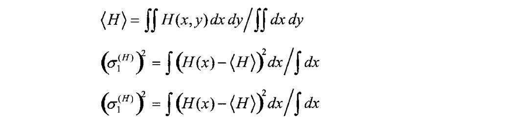
角速度ベクトルΩを次のように定義する。明るさのゆらぎ成分は+の値も-の値もどちらの値もとることが許されるので、角速度ベクトルとして許されるのは4つの状態が存在する。

このようにして、求めた剛体の静止状態における空間的な因子と剛体の運動を表す明るさの因子を用いて運動量を次のように定義する。
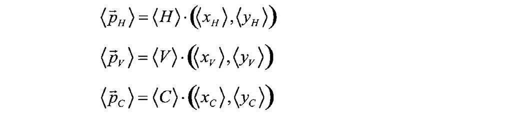
これらはベクトル成分を与えるが、運動量の要素pnとしては1つ1つのスカラー量に分解する。したがって、独立な運動量の要素の数は6つあることになる。
これらはベクトル成分を与えるが、運動量の要素pnとしては1つ1つのスカラー量に分解する。したがって、独立な運動量の要素の数は6つあることになる。
明るさの因子が運動の速度を表す物理的描像は次のような考え方である。ある画像を紙面上に提示したとすると、照明環境が真っ暗のとき、紙面上の画像そのものの性質は変わらないものの、人間の目には何も認識しない状態となる。そこへ照明電球をつけると、画像の色の明るさによって違った速度で目に画像の印象が飛び込んでくるが、その色としての着目領域は、画像の明るさの重心を中心として各色面毎に飛び込んでくる。ただし、その周りではいろいろな速度の違いを持った剛体の運動のように捉える。V面の場合は高輝度部ほど速い速度で強く目に飛び込んでくると考える。C面の場合は高彩度部ほど速い速度で強く目に飛び込んでくると考える。
7-4.角運動量の要素Mnの計算
剛体の静止状態における空間的な因子と剛体の運動を表す明るさの因子を用いて角運動量を次のように定義する。角速度ベクトルとして4つの状態が存在するが、その内、角運動量ベクトルとして独立な要素を与えるものだけを残す。すなわち、角運動量ベクトル全体に+、-の符号を付けるだけのものは、独立な状態と見なさない。テンソル記号はi番目のベクトル要素を求めるとき、全てのkについて和をとって縮約することを意味する。
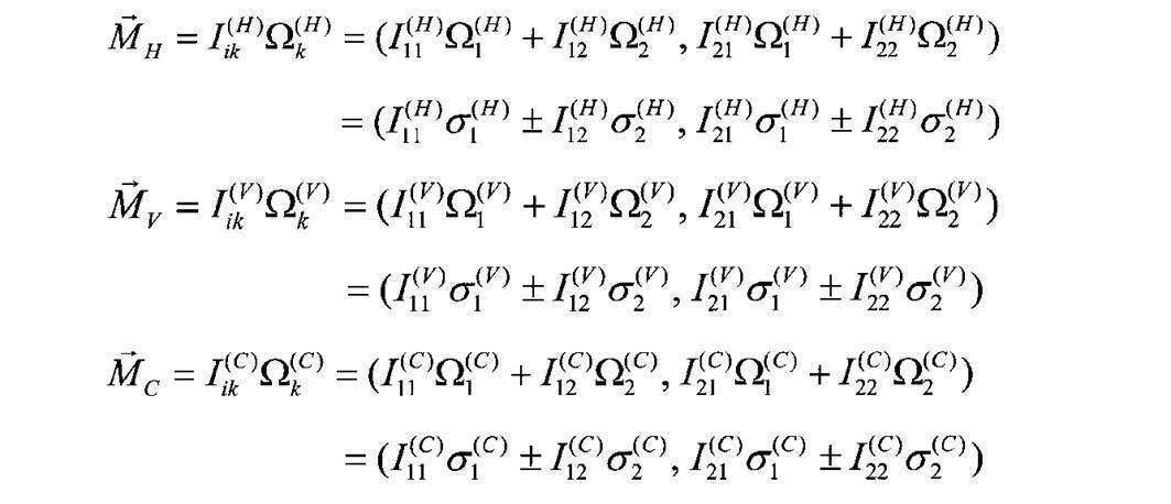
これらもベクトル成分を与えるが、角運動量の要素Mnとしては1つ1つのスカラー量に分解する。従って、独立な運動量の要素の数は12個あることになる。
剛体の静止状態における空間的な因子と剛体の運動を表す明るさの因子を用いて角運動量を次のように定義する。角速度ベクトルとして4つの状態が存在するが、その内、角運動量ベクトルとして独立な要素を与えるものだけを残す。すなわち、角運動量ベクトル全体に+、-の符号を付けるだけのものは、独立な状態と見なさない。テンソル記号はi番目のベクトル要素を求めるとき、全てのkについて和をとって縮約することを意味する。
これらもベクトル成分を与えるが、角運動量の要素Mnとしては1つ1つのスカラー量に分解する。従って、独立な運動量の要素の数は12個あることになる。
7-5.エネルギーの要素Enの計算
剛体の静止状態における空間的な因子と剛体の運動を表す明るさの因子を用いて角運動量を次のように定義する。角速度ベクトルとして4つの状態が存在するが、その内、エネルギーとして独立な要素を与えるものだけを残す。
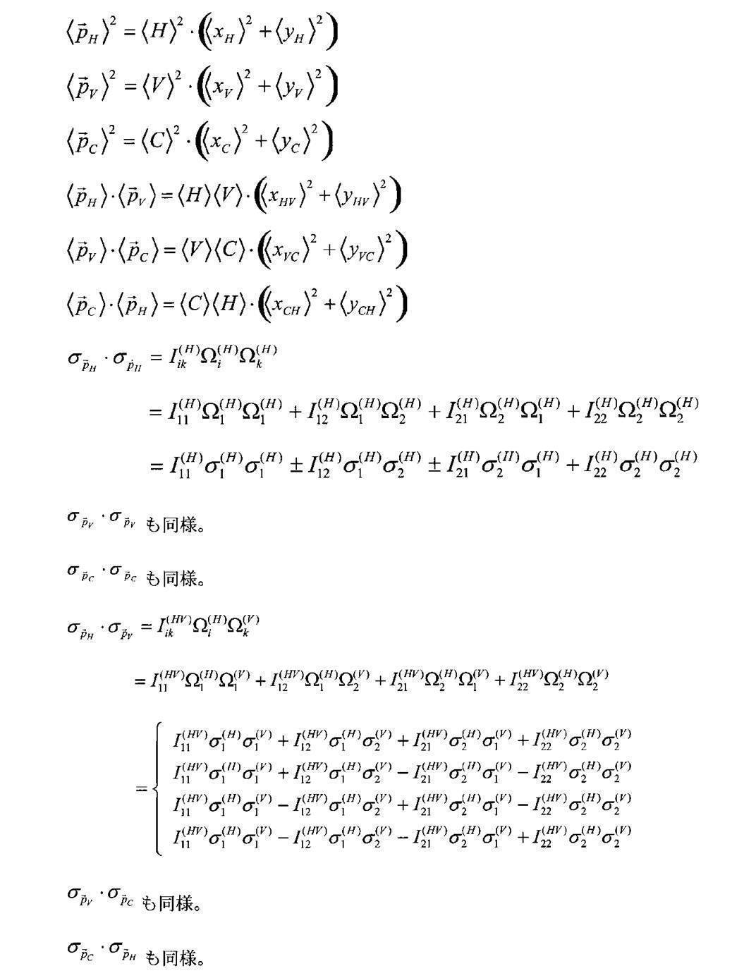
剛体の静止状態における空間的な因子と剛体の運動を表す明るさの因子を用いて角運動量を次のように定義する。角速度ベクトルとして4つの状態が存在するが、その内、エネルギーとして独立な要素を与えるものだけを残す。
独立なエネルギーの要素Enの数は、並進運動エネルギーを表す部分から6個、回転運動エネルギーを表す部分から18個で、合計24個となる。
第8の実施形態の冒頭で、モデル・ハミルトニアンを導いて展開したときに、状態の数として2倍の因子が出てくる(α)面と(β)面の積からなる項は、これらの定義に対して値を2倍にすると状態数を考慮したことになる。
第8の実施形態の冒頭で、モデル・ハミルトニアンを導いて展開したときに、状態の数として2倍の因子が出てくる(α)面と(β)面の積からなる項は、これらの定義に対して値を2倍にすると状態数を考慮したことになる。
これらの物理量が不変量になる性質を持っているのは次のような画像の性質を記述していることと関係する。風景写真の場合は、山々の連なりと青空が横方向に広がっていることが多い。すると、空間的な因子の慣性テンソルはx軸方向の広がりを表すI22が大きな値をとり、y軸方向の広がりを表すI11は小さな値をとりやすい。一方で、明るさ因子のゆらぎ幅に関して、青空と山との信号の大きさは随分と違う値をとるので、y軸に射影した方向のゆらぎ幅σ2は大きな値をとり、x軸方向に射影した方向のゆらぎ幅σ1は同質の画像領域で構成されるので小さな値をとりやすい。従って、I22とσ2との組み合わせは風景写真では大きな値となり、I11とσ1の組み合わせは小さな値をとりやすい。このような傾向が回転エネルギーの項や角運動量の要素として記述されることになる。また、人物系ではこれらは異なった値の傾向を示すことになる。従って、2次元色分布の構図の低次不変量はシーンを区別するよい特徴量となる。
7-6.部分系の温度の計算
第6の実施形態の3-6で示した手順と同様である。
7-7.部分系の自由エネルギーの計算
第6の実施形態の3-7で示した手順と同様である。
この部分系のボルツマン定数は、この部分系のエントロピーの任意の画像の統計平均の逆数で測る。

第6の実施形態の3-6で示した手順と同様である。
7-7.部分系の自由エネルギーの計算
第6の実施形態の3-7で示した手順と同様である。
この部分系のボルツマン定数は、この部分系のエントロピーの任意の画像の統計平均の逆数で測る。
なお、自由エネルギー、自由運動量、自由角運動量を定義するときに用いるエントロピーは、共通の位相空間上での状態数を測るものであるから、これまでの定義と同様に3者の間で共通のものを用いる。すなわち、エネルギーの要素を計算するために、例外的に導入した色面間の交差分布関数は、エントロピーへは関与しない。
8.二次元色分布の高次不変量の作成
この部分系を区別するための記号として不変量に対してHという記号を用いる場合がある。
8-0.低次系の分布関数のヒルベルト空間表現
HVC面の色面の2次元分布関数を、色の低次系の分布関数と位置づける。手順7-1で求めた剛体の分布関数である。低次系の分布関数は、元の座標系で測ることのできる座標空間qとも解釈することができる。これをルジャンドル陪関数で変換して周波数表現し、運動量空間pに投影する。これは元の分布関数を別の側面から見た等価表現である。ヒルベルト空間をなす基底関数として、低次系の分布関数の性質を加味して、できるだけコンパクトに表現する完全直交系の関数を選ぶ。しかし、座標空間と運動量空間の不確定性原理

によって、一方でコンパクト表現されているときは他方はブロードな表現となる関係にもある。その両者の不確定性が最小となるような関数系を選ぶのが最適である。
この部分系を区別するための記号として不変量に対してHという記号を用いる場合がある。
8-0.低次系の分布関数のヒルベルト空間表現
HVC面の色面の2次元分布関数を、色の低次系の分布関数と位置づける。手順7-1で求めた剛体の分布関数である。低次系の分布関数は、元の座標系で測ることのできる座標空間qとも解釈することができる。これをルジャンドル陪関数で変換して周波数表現し、運動量空間pに投影する。これは元の分布関数を別の側面から見た等価表現である。ヒルベルト空間をなす基底関数として、低次系の分布関数の性質を加味して、できるだけコンパクトに表現する完全直交系の関数を選ぶ。しかし、座標空間と運動量空間の不確定性原理
によって、一方でコンパクト表現されているときは他方はブロードな表現となる関係にもある。その両者の不確定性が最小となるような関数系を選ぶのが最適である。
本実施形態では、簡単のため二重級数展開を与えるルジャンドル陪関数の場合ではなく、その最低次(磁気量子数m=0)のみを扱い一重級数展開をあたえるルジャンドル関数の場合を示す。ルジャンドル陪関数の実施例は第9の実施形態で拡張して示す。
8-0-1.変数変換
2次元分布関数のx軸の座標範囲[xa,xb]、y軸の座標範囲[ya,yb]、分布関数の値(z軸とする)の範囲を[fa,fb]とすると、x軸を[-1,1]、y軸を[-1,1]、z軸を[-1,1]に収まる区間に変数変換を行う。この節の中だけ便宜的に、x軸の変数をXからxへ、y軸の変数をYからyへ、z軸の変数をfZからfzへ変換して表記すると、変換式は以下のようになる。
x軸の変数変換:x={X-(xb+xa)/2}/{(xb-xa)/2}
y軸の変数変換:y={Y-(yb+ya)/2}/{(yb-ya)/2}
z軸の変数変換:fz={fZ-(fb+fa)/2}/{(fb-fa)/2}
2次元分布関数のx軸の座標範囲[xa,xb]、y軸の座標範囲[ya,yb]、分布関数の値(z軸とする)の範囲を[fa,fb]とすると、x軸を[-1,1]、y軸を[-1,1]、z軸を[-1,1]に収まる区間に変数変換を行う。この節の中だけ便宜的に、x軸の変数をXからxへ、y軸の変数をYからyへ、z軸の変数をfZからfzへ変換して表記すると、変換式は以下のようになる。
x軸の変数変換:x={X-(xb+xa)/2}/{(xb-xa)/2}
y軸の変数変換:y={Y-(yb+ya)/2}/{(yb-ya)/2}
z軸の変数変換:fz={fZ-(fb+fa)/2}/{(fb-fa)/2}
8-0-2.ルジャンドル関数による級数展開
H,V,C各色面の2次元分布関数をN×N個の係数でルジャンドル関数で展開して等価表現する。

H,V,C各色面の2次元分布関数をN×N個の係数でルジャンドル関数で展開して等価表現する。
展開係数cll'は、基底関数の直交性を利用して、次のように求める。すなわち、2次元分布関数を一次元方向に対して各行毎に、直交変換した展開係数を求めた画像を生成し、今度はその面に対して直交する一次元方向の各列毎に、同様の変換を繰り返して、出来上がった面が2次元展開係数面cll'となる。各行毎、各列毎の一次元方向の展開は以下の関係式を用いて行う。
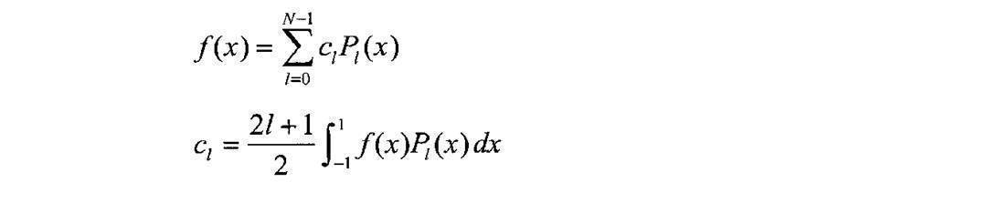
変数変換により展開係数の値は全て[-1,1]の範囲に収まる。展開係数の数は、色面の画像の画素数が360×240程度に対して、N=50程度に設定するとよい。x軸とy軸の展開の数は同じ値に設定しているので、展開係数は正方行列をなす。
8-1.高次系の分布関数の作成
ルジャンドル展開された係数のパワースペクトルを、構図の色に関する高次系の分布関数と定義する。H,V,C3面について、高次系の分布関数が定義できる。確率密度を表すように規格化しておく。

ルジャンドル展開された係数のパワースペクトルを、構図の色に関する高次系の分布関数と定義する。H,V,C3面について、高次系の分布関数が定義できる。確率密度を表すように規格化しておく。
8-2.エントロピーの計算
分布関数f(l,l')からエントロピーSを計算する。分布関数の色面を(α)で区別して表すと、H,V,C面の各々の分布関数からエントロピーが算出され、それらの和が2次元色分布の高次系に射影された部分系のエントロピーを表す。

この値をSHとする。
分布関数f(l,l')からエントロピーSを計算する。分布関数の色面を(α)で区別して表すと、H,V,C面の各々の分布関数からエントロピーが算出され、それらの和が2次元色分布の高次系に射影された部分系のエントロピーを表す。
この値をSHとする。
8-3.運動量の要素pnの計算
ルジャンドル関数による展開係数はヒルベルト空間における運動量と捉えることができる。従って、運動量の要素pnは展開係数

そのものである。
ルジャンドル関数による展開係数はヒルベルト空間における運動量と捉えることができる。従って、運動量の要素pnは展開係数
そのものである。
運動量の要素の数は、[]が配列を表すものとすると、
[α面の数][lの数][l'の数]=3x50x50
となる。これらを順にまとめてpnで表す。
[α面の数][lの数][l'の数]=3x50x50
となる。これらを順にまとめてpnで表す。
8-4.角運動量の要素Mnの計算
中心対称な形状の性質を与えるのは、展開係数の対角成分である。ルジャンドル関数の方位量子数l,l'がヒルベルト空間座標を規定するので、角運動量M=r×pをヒルベルト空間座標と運動量の積として定義する。
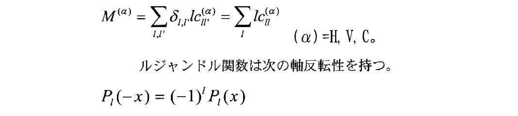
中心対称な形状の性質を与えるのは、展開係数の対角成分である。ルジャンドル関数の方位量子数l,l'がヒルベルト空間座標を規定するので、角運動量M=r×pをヒルベルト空間座標と運動量の積として定義する。
軸反転として4つの場合が存在するが、その内独立な要素を与えるのは、(α)(x,y)と(α')(x,-y)のみである。(α")(-x,y)は(α')(x,-y)と同じ状態を、(α"')(-x,-y)は(α)(x,y)と同じ状態を記述するにすぎない。y軸を反転したもう1つの独立な要素は以下の式で書ける。

角運動量の要素の数は、[]が配列を表すものとすると、
[α面の数][軸反転性の数]=3×2
となる。これらを順にまとめてMnで表す。
[α面の数][軸反転性の数]=3×2
となる。これらを順にまとめてMnで表す。
8-5.エネルギーの要素Enの計算
2次元展開係数

を12方向に並び替えた一次元配列を模式的に

で表すものとする。ベクトルkは並び替えの始点と方向を表し、それぞれに定義された並び替えの始点位置から係数を順に並び替え、0~N×N-1個の展開係数のi番目の展開係数をiによって表している。(α)面のi番目の展開係数ciと(β)面のj番目の展開係数cjを交換することによって、対称積と反対称積を作り、j-i=nの一定の量子数差をもったものの間で、全ての展開係数の和をとることによって、エネルギー準位Enの要素の値を作る。

2次元展開係数
を12方向に並び替えた一次元配列を模式的に
で表すものとする。ベクトルkは並び替えの始点と方向を表し、それぞれに定義された並び替えの始点位置から係数を順に並び替え、0~N×N-1個の展開係数のi番目の展開係数をiによって表している。(α)面のi番目の展開係数ciと(β)面のj番目の展開係数cjを交換することによって、対称積と反対称積を作り、j-i=nの一定の量子数差をもったものの間で、全ての展開係数の和をとることによって、エネルギー準位Enの要素の値を作る。
ここに、cjの値がcN×N-1+iのように0~N×N-1個の定義域からはみ出したとき、一次元化した展開係数の最後と最初を円環につないで、最初の地点に戻って定義し直すものとする。すなわち、cN×N-1+i=ciとする。
エネルギー準位数nは2次元展開係数のライン上の性質だけを調べるので、量子数の差がn=0,1,...,N-1までのものをとる。

は12×12通りの組み合わせのエネルギー分散関係、すなわち、kiとkjの組み合わせを表すk空間上の点n=j-iにおいて、そのk点上で如何なるエネルギー値をとっているかという関係式を記述する。
エネルギー準位数nは2次元展開係数のライン上の性質だけを調べるので、量子数の差がn=0,1,...,N-1までのものをとる。
は12×12通りの組み合わせのエネルギー分散関係、すなわち、kiとkjの組み合わせを表すk空間上の点n=j-iにおいて、そのk点上で如何なるエネルギー値をとっているかという関係式を記述する。
(α)面と(α)面の対称積の定義に対して、12×12方向の組み合わせが全く同じ方向同士になる12通りの組み合わせの内、n=j-i=0の点だけは分子と分母が同じ値になるので、例外的に分子だけの定義とする。すなわち、

零点エネルギーのオフセットを入れているが、1の値を超えてもそのまま状態の数を記述しているという意味で、実際にはこのような補正は入れずに、自己相関値をそのまま使うとよい。同じ考え方は、チェビシェフ展開係数や球ベッセル展開係数から作成したエネルギーの場合についても当てはまる。
軸反転性に関して、α面とβ面のそれぞれの4つの状態に対して、展開係数が以下のように入れ替わるので、上述の定義のエネルギー分散関係は、さらに4×4倍のエネルギー分散関係が独立に定義できる。
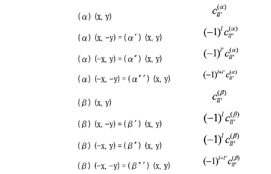
エネルギーの要素の数は、[]が配列を表すものとすると、
[α面とβ面の組み合わせの数][α面の軸反転性の数][β面の軸反転性の数][α面の並び替え方の数][β面の並び替え方の数][対称積か反対称積かの種別][エネルギー準位数]
=6×4×4×12×12×2×50
となる。これらを順にまとめてEnで表す。
[α面とβ面の組み合わせの数][α面の軸反転性の数][β面の軸反転性の数][α面の並び替え方の数][β面の並び替え方の数][対称積か反対称積かの種別][エネルギー準位数]
=6×4×4×12×12×2×50
となる。これらを順にまとめてEnで表す。
α面とβ面の組み合わせとしてはHH,VV,CC,HV,VC,CHの6通りであるが、HV,VC,CHはVH,CV,HCの組み合わせと共通であるので、独立な要素ではないが、状態数としては(α)(α)に対して(α)(β)が2倍存在しているので、エネルギー値としては定義値に対して後から2倍する。
これらのエネルギー要素をそのまま用いてもよいが、もっと縮約されたエネルギー分散関係を求める方が実用的な場合がある。その場合の方法を述べる。

は12×12通りの組み合わせのエネルギー分散関係を導出しているが、これらの方向組み合わせに関して、同じエネルギー準位En同士で平均的なエネルギー分散関係を求める。このような操作をすると、反対称積の平均的なエネルギー分散関係は恒等的に零となる。従って、対称積側のエネルギー分散関係だけが残ることになる。
は12×12通りの組み合わせのエネルギー分散関係を導出しているが、これらの方向組み合わせに関して、同じエネルギー準位En同士で平均的なエネルギー分散関係を求める。このような操作をすると、反対称積の平均的なエネルギー分散関係は恒等的に零となる。従って、対称積側のエネルギー分散関係だけが残ることになる。

このようにすると、エネルギー要素の数は、
[α面とβ面の組み合わせの数][α面の軸反転性の数][β面の軸反転性の数][エネルギー準位数]
=6×4×4×50
となる。これらを順にまとめてEnで表す。
例として、VV面同士の対称積のエネルギー準位n=0付近のエネルギー要素に関して、どのような画像を区別する能力を有するのかを、画像整列によって調べてみると、一方には社寺などの構造物系の写真画像が集まりやすく、他方には湖沼などの自然風景の写真画像が集まりやすいという分類能力を有する。また、軸反転したものは異なった性質の画像を分類する能力を有する。
8-6.部分系の温度の計算
第6の実施形態の4-6で示した手順と同様である。
8-7.部分系の自由エネルギーの計算
第6の実施形態の4-7で示した手順と同様である。
この部分系のボルツマン定数は、この部分系のエントロピーの任意の画像の統計平均の逆数で測る。

第6の実施形態の4-6で示した手順と同様である。
8-7.部分系の自由エネルギーの計算
第6の実施形態の4-7で示した手順と同様である。
この部分系のボルツマン定数は、この部分系のエントロピーの任意の画像の統計平均の逆数で測る。
9.二次元エッジ分布の低次不変量の作成
この部分系を区別するための記号として不変量に対してIoという記号を用いる場合がある。
9-1.低次系の分布関数の作成
第2の実施形態でウェーブレット変換することによって多重解像度の高周波サブバンドを生成し、高周波サブバンドのみを最低解像度より逆ウェーブレット変換を行いエッジ統合する説明をしている。多重解像度の段数は、最低解像度が40×30~80×60程度の画像範囲に入る程度まで分解しているので、最低解像度から3段程度高解像度に位置する320×240画素程度の統合エッジ画像をエッジ面として取り出す。HVC各色面について取り出し、それぞれの信号面をΔH(x,y),ΔV(x,y),ΔC(x,y)と表す。ここで用いている色相面もニュートラルの分離を行っていない色面である。
これらのエッジ面の画像は正と負の値を持っているので分布関数とは呼べない。エッジ面を2乗したものをエッジ面の2次元分布関数として定義し、これらの分布を剛体面と捉えて、剛体が持つ空間的な因子に関する性質を調べるために用いる。この剛体面は、色の2次元分布の場合と異なり、輪郭線にのみ強度を持つスケルトン画像である。

色面間の交差する分布関数f(HV)(x,y)、f(VC)(x,y)、f(CH)(x,y)は手順7-1と同様に定義する。
色面間の交差する分布関数f(HV)(x,y)、f(VC)(x,y)、f(CH)(x,y)は手順7-1と同様に定義する。
9-2.エントロピーの計算
エッジ面の分布関数f(x,y)からエントロピーSを計算する。分布関数の値が0のところは、その状態をとらないという意味で、積分区間から排除する。エッジ面の分布関数の色面を(α)で区別して表すと、H,V,C面の各々の分布関数からエントロピーが算出され、それらの和が2次元エッジ分布の低次系に射影された部分系のエントロピーを表す。

この値をSIoとする。
エッジ面の分布関数f(x,y)からエントロピーSを計算する。分布関数の値が0のところは、その状態をとらないという意味で、積分区間から排除する。エッジ面の分布関数の色面を(α)で区別して表すと、H,V,C面の各々の分布関数からエントロピーが算出され、それらの和が2次元エッジ分布の低次系に射影された部分系のエントロピーを表す。
この値をSIoとする。
9-3.運動量の要素pnの計算
空間的な形状因子に関する計算は、統合エッジ面を2乗した面を用いて計算するが、明るさ因子に関する計算は、統合エッジ面の値そのものを用いて計算する。なぜならば、明るさ因子に関しては、正負の値自体に意味があり、エッジ強度が正の領域はこちらに向かって正の速度で目に飛び込んでくるが、負の領域は後退する速度で逆方向に向かっていると認識するのが知覚の記述に合致しているからである。
空間的な形状の重心位置は、エッジ面としての注目領域を与えるが、この注目領域は色面の重心位置と異なる。すなわち、色とエッジでは着目している領域が異なる。
以下に、エッジ面の場合の対応式を羅列する。手順9-5まで続けて行う。
空間的な形状因子に関する計算は、統合エッジ面を2乗した面を用いて計算するが、明るさ因子に関する計算は、統合エッジ面の値そのものを用いて計算する。なぜならば、明るさ因子に関しては、正負の値自体に意味があり、エッジ強度が正の領域はこちらに向かって正の速度で目に飛び込んでくるが、負の領域は後退する速度で逆方向に向かっていると認識するのが知覚の記述に合致しているからである。
空間的な形状の重心位置は、エッジ面としての注目領域を与えるが、この注目領域は色面の重心位置と異なる。すなわち、色とエッジでは着目している領域が異なる。
以下に、エッジ面の場合の対応式を羅列する。手順9-5まで続けて行う。
空間的な形状因子
1つの色面内の分布に関する重心位置と慣性テンソルの記述の場合。
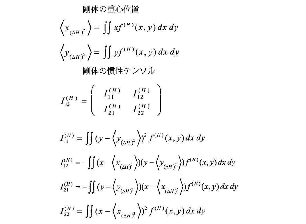
2つの色面間で交差する分布に関する重心位置と慣性テンソルの記述の場合。
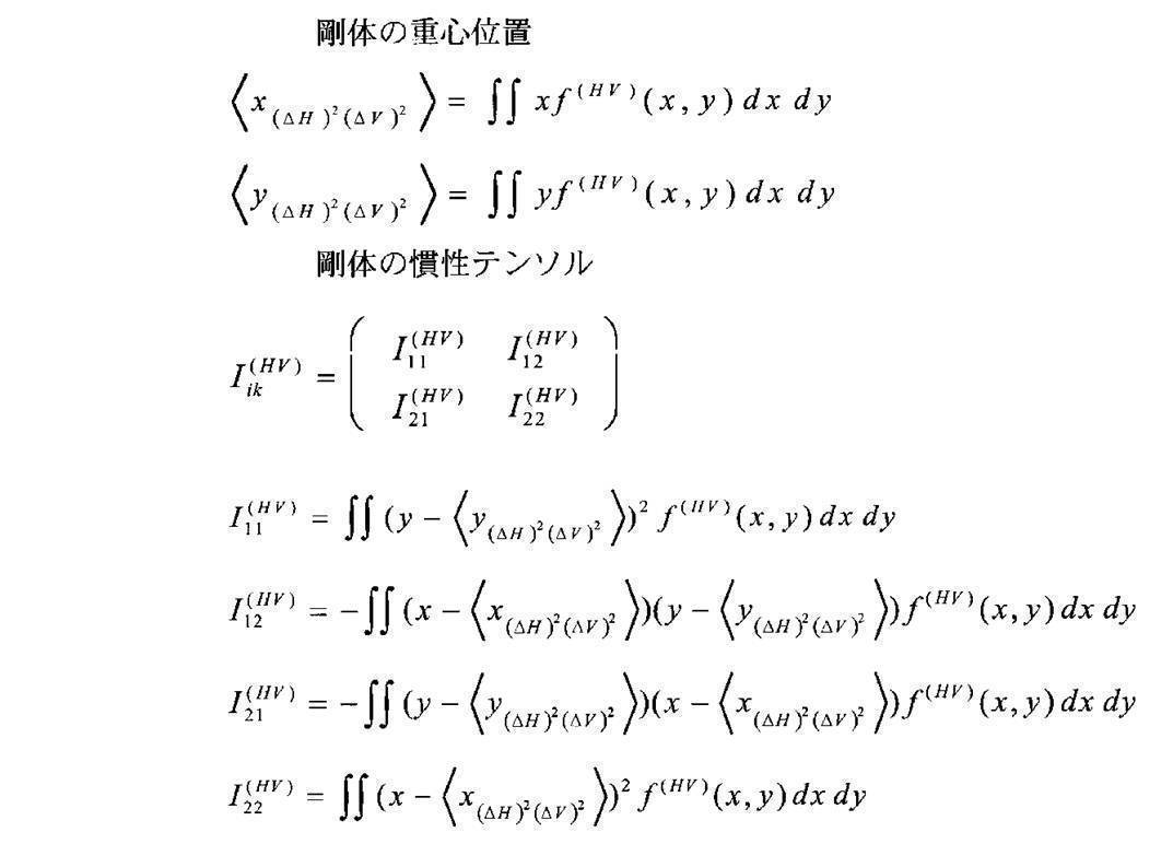
1つの色面内の分布に関する重心位置と慣性テンソルの記述の場合。
2つの色面間で交差する分布に関する重心位置と慣性テンソルの記述の場合。
明るさの因子
y軸方向に平均操作をしてx軸に射影した画像を△H(x)、x軸方向に平均操作をしてy軸に射影した画像を△H(y)とする。さらに△H面全体の平均値<△H>も算出する。
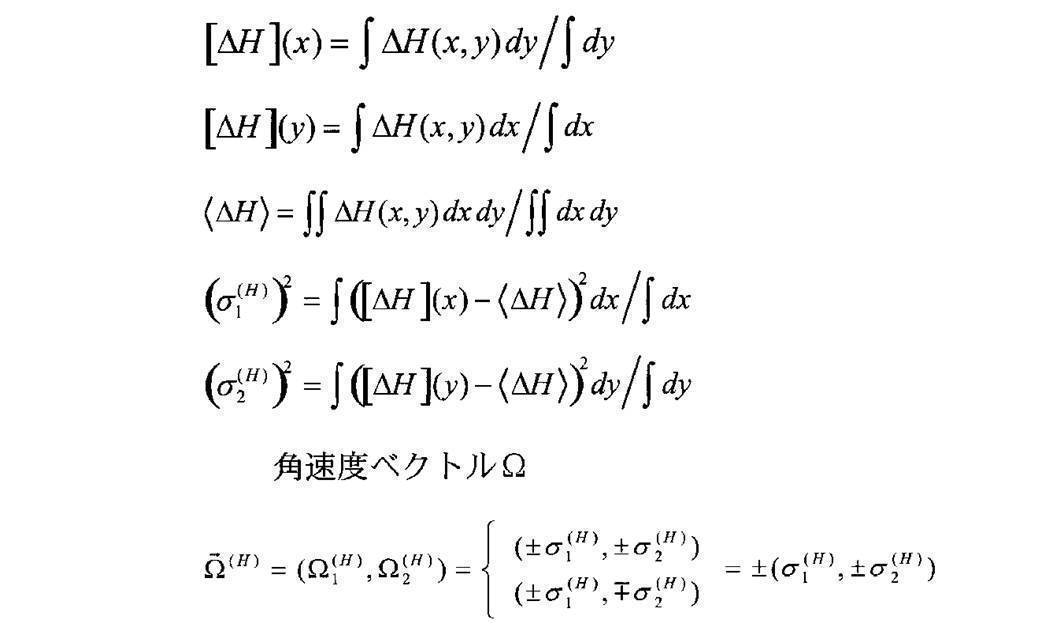
y軸方向に平均操作をしてx軸に射影した画像を△H(x)、x軸方向に平均操作をしてy軸に射影した画像を△H(y)とする。さらに△H面全体の平均値<△H>も算出する。
運動量の要素の計算
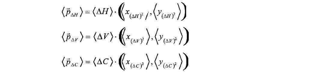
9-4.角運動量の要素Mnの計算

9-5.エネルギーの要素Enの計算

9-6.部分系の温度の計算
第6の実施形態の手順5と同様である。
9-7.部分系の自由エネルギーの計算
第6の実施形態の手順5と同様である。
この部分系のボルツマン定数は、この部分系のエントロピーの任意の画像の統計平均の逆数で測る。

第6の実施形態の手順5と同様である。
9-7.部分系の自由エネルギーの計算
第6の実施形態の手順5と同様である。
この部分系のボルツマン定数は、この部分系のエントロピーの任意の画像の統計平均の逆数で測る。
10.二次元エッジ分布の高次不変量の作成
この部分系を区別するための記号として不変量に対してIという記号を用いる場合がある。
10-0.低次系の分布関数のヒルベルト空間表現
HVC面のエッジ面の2次元分布関数を、エッジの低次系の分布関数と位置づける。手順9-1で求めた剛体の分布関数である。低次系の分布関数は、元の座標系で測ることのできる座標空間qとも解釈することができる。これをフーリエ関数で変換して周波数表現し、運動量空間pに投影する。これは元の分布関数を別の側面から見た等価表現である。ヒルベルト空間をなす基底関数として、低次系の分布関数の性質を加味して、できるだけコンパクトに表現する完全直交系の関数を選ぶ。しかし、座標空間と運動量空間の不確定性原理

によって、一方でコンパクト表現されているときは他方はブロードな表現となる関係にもある。その両者の不確定性が最小となるような関数系を選ぶのが最適である。
この部分系を区別するための記号として不変量に対してIという記号を用いる場合がある。
10-0.低次系の分布関数のヒルベルト空間表現
HVC面のエッジ面の2次元分布関数を、エッジの低次系の分布関数と位置づける。手順9-1で求めた剛体の分布関数である。低次系の分布関数は、元の座標系で測ることのできる座標空間qとも解釈することができる。これをフーリエ関数で変換して周波数表現し、運動量空間pに投影する。これは元の分布関数を別の側面から見た等価表現である。ヒルベルト空間をなす基底関数として、低次系の分布関数の性質を加味して、できるだけコンパクトに表現する完全直交系の関数を選ぶ。しかし、座標空間と運動量空間の不確定性原理
によって、一方でコンパクト表現されているときは他方はブロードな表現となる関係にもある。その両者の不確定性が最小となるような関数系を選ぶのが最適である。
10-0-1.変数変換
2次元分布関数のx軸の座標範囲[xa,xb]、y軸の座標範囲[ya,yb]、分布関数の値(z軸とする)の範囲を[fa,fb]とすると、x軸を[-π,π]、y軸を[-π,π]、z軸を[0,1]に収まる区間に変数変換を行う。この節の中だけ便宜的に、x軸の変数をXからxへ、y軸の変数をYからyへ、z軸の変数をfZからfzへ変換して表記すると、変換式は以下のようになる。
x軸の変数変換:x=π{X-(xb+xa)/2}/{(xb-xa)/2}
y軸の変数変換:y=π{Y-(yb+ya)/2}/{(yb-ya)/2}
z軸の変数変換:fz=(fZ-fa)/(fb-fa)
通常fa=0の値をとる。
2次元分布関数のx軸の座標範囲[xa,xb]、y軸の座標範囲[ya,yb]、分布関数の値(z軸とする)の範囲を[fa,fb]とすると、x軸を[-π,π]、y軸を[-π,π]、z軸を[0,1]に収まる区間に変数変換を行う。この節の中だけ便宜的に、x軸の変数をXからxへ、y軸の変数をYからyへ、z軸の変数をfZからfzへ変換して表記すると、変換式は以下のようになる。
x軸の変数変換:x=π{X-(xb+xa)/2}/{(xb-xa)/2}
y軸の変数変換:y=π{Y-(yb+ya)/2}/{(yb-ya)/2}
z軸の変数変換:fz=(fZ-fa)/(fb-fa)
通常fa=0の値をとる。
10-0-2.フーリエ関数による級数展開
H,V,C各色面の2次元分布関数を(2M+2)×(2M+2)個の係数で余弦関数と正弦関数の組からなるフーリエ関数で展開して等価表現する。

H,V,C各色面の2次元分布関数を(2M+2)×(2M+2)個の係数で余弦関数と正弦関数の組からなるフーリエ関数で展開して等価表現する。
展開係数Amm',Bmm',Cmm',Dmm'は、基底関数の直交性を利用して、次のように求める。すなわち、2次元分布関数を一次元方向に対して各行毎に、直交変換した展開係数を求めた画像を生成し、今度はその面に対して直交する一次元方向の各列毎に、同様の変換を繰り返して、出来上がった面が2次元展開係数面Amm',Bmm',Cmm',Dmm'となる。各行毎、各列毎の一次元方向の展開は以下の関係式を用いて行う。
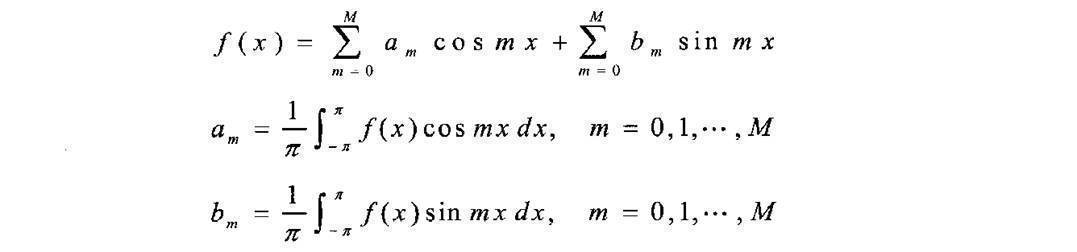
ただし、a0=a0/2とする。b0=0である。従って、Bm0=0、C0m'=0、Dm0=D0m'=0である。
ただし、a0=a0/2とする。b0=0である。従って、Bm0=0、C0m'=0、Dm0=D0m'=0である。
変数変換により展開係数の値は全て[-1,1]の範囲に収まる。展開係数の数は、エッジ面の画像の画素数が360×240程度に対して、M=25程度に設定するとよい。x軸とy軸の展開の数は同じ値に設定しているので、展開係数は正方行列をなす。
ここで、4つの展開係数の行列Amm',Bmm',Cmm',Dmm'をamm'として1つの行列にまとめてしまうのが便利である。x軸、y軸のそれぞれの最も高い周波数が最も低い周波数と接続して同じ性質を表すというk空間におけるブリルアンゾーンの性質を備えた並び替え方としては、次のようなまとめ方がある。本実施形態では、通常これを用いる。
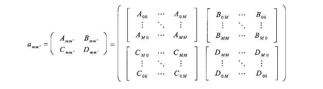
他にも、最も左上にD00を、その右隣にB00を、D00の下にC00を、B00の下にA00を並べ、この4つを基本単位として縦方向と横方向に数を1つずつ繰り上げ、2行2列ずつ増やしていく並べ方も存在する。これも最低周波数と最高周波数が接続する性質を持つ。
両者とも行列共に正の量子数で表されたk空間で表現されているものを、半分の地点で折り返して、はみ出した部分を負の領域として記述しても全く等価な表現となる。これがブリルアンゾーンの性質である。
両者とも行列共に正の量子数で表されたk空間で表現されているものを、半分の地点で折り返して、はみ出した部分を負の領域として記述しても全く等価な表現となる。これがブリルアンゾーンの性質である。
10-1.高次系の分布関数の作成
フーリエ展開された係数のパワースペクトルを、構図のエッジに関する高次系の分布関数と定義する。H,V,C3面について、高次系の分布関数が定義できる。確率密度を表すように規格化しておく。

フーリエ展開された係数のパワースペクトルを、構図のエッジに関する高次系の分布関数と定義する。H,V,C3面について、高次系の分布関数が定義できる。確率密度を表すように規格化しておく。
10-2.エントロピーの計算
分布関数f(m,m')からエントロピーSを計算する。分布関数の色面を(α)で区別して表すと、H,V,C面の各々の分布関数からエントロピーが算出され、それらの和が2次元エッジ分布の高次系に射影された部分系のエントロピーを表す。

この値をSIとする。
分布関数f(m,m')からエントロピーSを計算する。分布関数の色面を(α)で区別して表すと、H,V,C面の各々の分布関数からエントロピーが算出され、それらの和が2次元エッジ分布の高次系に射影された部分系のエントロピーを表す。
この値をSIとする。
10-3.運動量の要素pnの計算
フーリエ関数による展開係数はヒルベルト空間における運動量と捉えることができる。したがって、運動量の要素pnは展開係数Amm',Bmm',Cmm',Dmm'そのものである。
運動量の要素の数は、[]が配列を表すものとすると、
[α面の数][ABCDの種類][mの数][m'の数]=3×4×26×26
となる。これらを順にまとめてpnで表す。
フーリエ関数による展開係数はヒルベルト空間における運動量と捉えることができる。したがって、運動量の要素pnは展開係数Amm',Bmm',Cmm',Dmm'そのものである。
運動量の要素の数は、[]が配列を表すものとすると、
[α面の数][ABCDの種類][mの数][m'の数]=3×4×26×26
となる。これらを順にまとめてpnで表す。
10-4.角運動量の要素Mnの計算
中心対称な形状の性質を与えるのは、展開係数amm'の対角成分である。フーリエ関数の磁気量子数m,m'がヒルベルト空間座標を規定するので、角運動量M=rxpをヒルベルト空間座標と運動量の積として定義する。

中心対称な形状の性質を与えるのは、展開係数amm'の対角成分である。フーリエ関数の磁気量子数m,m'がヒルベルト空間座標を規定するので、角運動量M=rxpをヒルベルト空間座標と運動量の積として定義する。
フーリエ関数は次の軸反転性を持つ。

軸反転として4つの場合が存在するが、その内独立な要素を与えるのは、(α)(x,y)と(α')(x,-y)のみである。(α")(-x,y)は(α')(x,-y)と同じ状態を、(α"')(-x,-y)は(α)(x,y)と同じ状態を記述するにすぎない。y軸を反転したもう1つの独立な要素は以下の式で書ける。

角運動量の要素の数は、[]が配列を表すものとすると、
[α面の数][軸反転性の数]=3×2
となる。これらを順にまとめてMnで表す。
角運動量の要素の数は、[]が配列を表すものとすると、
[α面の数][軸反転性の数]=3×2
となる。これらを順にまとめてMnで表す。
10-5.エネルギーの要素Enの計算
2次元展開係数

を12方向に並び替えた一次元配列を模式的に

で表すものとする。ベクトルkは並び替えの始点と方向を表し、それぞれに定義された並び替えの始点位置から係数を順に並び替え、0~(2M+2)×(2M+2)-1個の展開係数のi番目の展開係数をiによって表している。(α)面のi番目の展開係数aiと(β)面のj番目の展開係数ajを交換することによって、対称積と反対称積を作り、j-i=nの一定の量子数差をもったものの間で、全ての展開係数の和をとることによって、エネルギー準位Enの要素の値を作る。

2次元展開係数
を12方向に並び替えた一次元配列を模式的に
で表すものとする。ベクトルkは並び替えの始点と方向を表し、それぞれに定義された並び替えの始点位置から係数を順に並び替え、0~(2M+2)×(2M+2)-1個の展開係数のi番目の展開係数をiによって表している。(α)面のi番目の展開係数aiと(β)面のj番目の展開係数ajを交換することによって、対称積と反対称積を作り、j-i=nの一定の量子数差をもったものの間で、全ての展開係数の和をとることによって、エネルギー準位Enの要素の値を作る。
ここに、ajの値がa(2M+2)×(2m+2)-1+iのように0~(2M+2)x(2M+2)-1個の定義域からはみ出したとき、一次元化した展開係数の最後と最初を円環につないで、最初の地点に戻って定義し直すものとする。すなわち、a(2M+2)x(2m+2)-1+i=aiとする。
エネルギー準位数nは2次元展開係数のライン上の性質だけを調べるので、量子数の差がn=0,1,...,(2M+2)-1までのものをとる。

は12×12通りの組み合わせのエネルギー分散関係、すなわち、kiとkjの組み合わせを表すk空間上の点n=j-iにおいて、そのk点上で如何なるエネルギー値をとっているかという関係式を記述する。
エネルギー準位数nは2次元展開係数のライン上の性質だけを調べるので、量子数の差がn=0,1,...,(2M+2)-1までのものをとる。
は12×12通りの組み合わせのエネルギー分散関係、すなわち、kiとkjの組み合わせを表すk空間上の点n=j-iにおいて、そのk点上で如何なるエネルギー値をとっているかという関係式を記述する。
(α)面と(α)面の対称積の定義に対して、12×12方向の組み合わせが全く同じ方向同士になる12通りの組み合わせの内、n=j-i=0の点だけは分子と分母が同じ値になるので、例外的に分子だけの定義とする。すなわち、

零点エネルギーのオフセットを入れているが、1の値を超えてもそのまま状態の数を記述しているという意味で、実際にはこのような補正は入れずに、自己相関値をそのまま使うとよい。
軸反転性に関して、α面とβ面のそれぞれの4つの状態に対して、展開係数

が以下のように入れ替わるので、上述の定義のエネルギー分散関係は、さらに4x4倍のエネルギー分散関係が独立に定義できる。
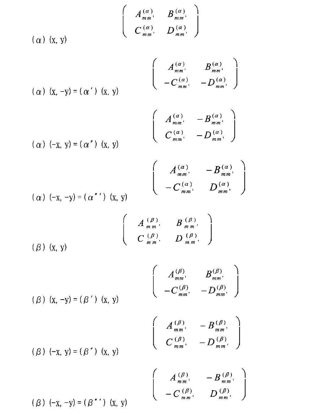
軸反転性に関して、α面とβ面のそれぞれの4つの状態に対して、展開係数
が以下のように入れ替わるので、上述の定義のエネルギー分散関係は、さらに4x4倍のエネルギー分散関係が独立に定義できる。
エネルギーの要素の数は、[]が配列を表すものとすると、
[α面とβ面の組み合わせの数][α面の軸反転性の数][β面の軸反転性の数][α面の並び替え方の数][β面の並び替え方の数][対称積か反対称積かの種別][エネルギー準位数]
=6×4×4×12×12×2×52
となる。これらを順にまとめてEnで表す。
[α面とβ面の組み合わせの数][α面の軸反転性の数][β面の軸反転性の数][α面の並び替え方の数][β面の並び替え方の数][対称積か反対称積かの種別][エネルギー準位数]
=6×4×4×12×12×2×52
となる。これらを順にまとめてEnで表す。
この場合も、もっと縮約されたエネルギー分散関係を求める。

は12×12通りの組み合わせのエネルギー分散関係を導出しているが、これらの方向組み合わせに関して、同じエネルギー準位En同士で平均的なエネルギー分散関係を求める。このような操作をすると、反対称積の平均的なエネルギー分散関係は恒等的に零となる。従って、対称積側のエネルギー分散関係だけが残ることになる。

は12×12通りの組み合わせのエネルギー分散関係を導出しているが、これらの方向組み合わせに関して、同じエネルギー準位En同士で平均的なエネルギー分散関係を求める。このような操作をすると、反対称積の平均的なエネルギー分散関係は恒等的に零となる。従って、対称積側のエネルギー分散関係だけが残ることになる。
こうすると、エネルギー要素の数は、
[α面とβ面の組み合わせの数][α面の軸反転性の数][β面の軸反転性の数][エネルギー準位数]
=6×4×4×52
となる。これらを順にまとめてEnで表す。
例として、VV面同士の対称積のエネルギー準位n=0付近のエネルギー要素に関して、どのような画像を区別する能力があるのかを、画像整列によって調べてみると、一方には風景などの自然系の写真画像が集まりやすく、他方には人物などの雑踏系の写真画像が集まりやすいという分類能力を有する。また、軸反転したものはまた異なった性質の画像を分類する能力を持つ。
[α面とβ面の組み合わせの数][α面の軸反転性の数][β面の軸反転性の数][エネルギー準位数]
=6×4×4×52
となる。これらを順にまとめてEnで表す。
例として、VV面同士の対称積のエネルギー準位n=0付近のエネルギー要素に関して、どのような画像を区別する能力があるのかを、画像整列によって調べてみると、一方には風景などの自然系の写真画像が集まりやすく、他方には人物などの雑踏系の写真画像が集まりやすいという分類能力を有する。また、軸反転したものはまた異なった性質の画像を分類する能力を持つ。
10-6.部分系の温度の計算
第6の実施形態の4-6で示した手順と同様である。
10-7.部分系の自由エネルギーの計算
第6の実施形態の4-7で示した手順と同様である。
この部分系のボルツマン定数は、この部分系のエントロピーの任意の画像の統計平均の逆数で測る。

第6の実施形態の4-6で示した手順と同様である。
10-7.部分系の自由エネルギーの計算
第6の実施形態の4-7で示した手順と同様である。
この部分系のボルツマン定数は、この部分系のエントロピーの任意の画像の統計平均の逆数で測る。
11.部分系の力学的不変量単位の統合
11-1.形容詞の設定
11-2.一般画像モデルの構築
11-3.形容詞モデル画像の構築
11-4.要素内の分布における偏差値の算出
11-5.部分系の力学的不変量単位の部分エネルギー、部分運動量、部分角運動量の算出
12.部分系の形容詞エネルギーへの統合
13.全系の形容詞エネルギーへの統合
14.形容詞検索処理
手順11から14までは、第6の実施形態と全く同じ手順を踏む。
11-1.形容詞の設定
11-2.一般画像モデルの構築
11-3.形容詞モデル画像の構築
11-4.要素内の分布における偏差値の算出
11-5.部分系の力学的不変量単位の部分エネルギー、部分運動量、部分角運動量の算出
12.部分系の形容詞エネルギーへの統合
13.全系の形容詞エネルギーへの統合
14.形容詞検索処理
手順11から14までは、第6の実施形態と全く同じ手順を踏む。
こうして、色とエッジの階調に関する一次元分布と、色とエッジの構図に関する2次元分布から導かれる感性不変量、あるいは画像認識に関わる不変量が共通土俵で相加的な特徴量として記述されたことになる。ある形容詞の認識においてある特徴が深く関わる場合には、その特徴量が一般画像に対して大きな偏差をもって記述されることになる。射影空間表現という考え方をとっているので、人間の認識構造、感性構造を可視化することができる。周波数記述におけるエネルギーバンド図の一部を2つの形容詞を比較して示している。
[第9の実施形態]
第8の実施形態に対して、色の2次元分布関数の高次系不変量を記述するときに、ルジャンドル陪関数展開がm=0,1,2,3の場合の例を示す。
8.二次元色分布の高次不変量の作成
8-0.低次系の分布関数のヒルベルト空間表現
8-0-1.変数変換
8-0-2.ルジャンドル陪関数による級数展開
H,V,C各色面の2次元分布関数をN×N個の係数でルジャンドル陪関数で2重級数展開して等価表現する。

第8の実施形態に対して、色の2次元分布関数の高次系不変量を記述するときに、ルジャンドル陪関数展開がm=0,1,2,3の場合の例を示す。
8.二次元色分布の高次不変量の作成
8-0.低次系の分布関数のヒルベルト空間表現
8-0-1.変数変換
8-0-2.ルジャンドル陪関数による級数展開
H,V,C各色面の2次元分布関数をN×N個の係数でルジャンドル陪関数で2重級数展開して等価表現する。
まず、磁気量子数に関するm×m'通りの一重級数展開による等価表現をする。

展開係数cmm ll'は、基底関数の直交性を利用して求める。各行毎、各列毎の一次元方向の展開は以下の関係式を用いて行う。
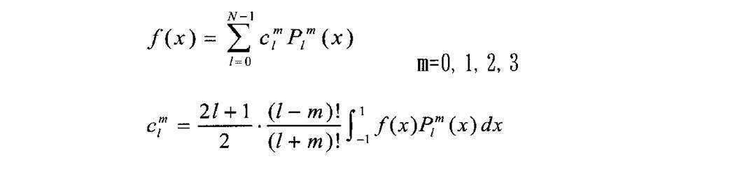
展開係数cmm ll'は、基底関数の直交性を利用して求める。各行毎、各列毎の一次元方向の展開は以下の関係式を用いて行う。
二重級数展開するときの磁気量子数間の重みamm'は均等配分の1とする。磁気量子数mの間の直交性は、色面の2次元分布関数

とエッジ面の2次元分布関数

を2つの分布関数の積によって同時展開したとき、エッジ面の2次元分布関数のフーリエ関数の直交性によって保証される。
とエッジ面の2次元分布関数
を2つの分布関数の積によって同時展開したとき、エッジ面の2次元分布関数のフーリエ関数の直交性によって保証される。
この部分系の不変量の計算に使う展開係数cmm'll'は、一重級数で求まった展開係数cmm
ll'と等しくなる。こうして、m×m'通り、すなわち磁気量子数に関して4×4通りの正方行列が生成される。
8-1.高次系の分布関数の作成

8-2.エントロピーの計算

8-3.運動量の要素pnの計算
運動量の要素pnは展開係数

そのものである。
運動量の要素の数は、[]が配列を表すものとすると、
[α面の数][mの数][m'の数][lの数][l'の数]=3×4×4×50×50
となる。これらを順にまとめてpnで表す。
運動量の要素pnは展開係数
そのものである。
運動量の要素の数は、[]が配列を表すものとすると、
[α面の数][mの数][m'の数][lの数][l'の数]=3×4×4×50×50
となる。これらを順にまとめてpnで表す。
8-4.角運動量の要素Mnの計算
ルジャンドル陪関数の展開係数の中で、中心対称な形状の性質を与えるのは、磁気量子数m,m'が共に等しく、その磁気量子数の組における方位量子数l,l'に関する展開係数の対角成分であるとする。ルジャンドル陪関数の方位量子数l,l'がヒルベルト空間座標を規定するとして、角運動量M=r×pをヒルベルト空間座標と運動量の積として定義する。

ルジャンドル陪関数の展開係数の中で、中心対称な形状の性質を与えるのは、磁気量子数m,m'が共に等しく、その磁気量子数の組における方位量子数l,l'に関する展開係数の対角成分であるとする。ルジャンドル陪関数の方位量子数l,l'がヒルベルト空間座標を規定するとして、角運動量M=r×pをヒルベルト空間座標と運動量の積として定義する。
ルジャンドル陪関数は次の軸反転性を持つ。

軸反転として4つの場合が存在するが、その内独立な要素を与えるのは、(α)(x,y)と(α')(x,-y)のみである。(α")(-x,y)は(α')(x,-y)と同じ状態を、(α"')(-x,-y)は(α)(x,y)と同じ状態を記述するにすぎない。y軸を反転したもう1つの独立な要素は以下の式で書ける。

角運動量の要素の数は、[]が配列を表すものとすると、
[α面の数][軸反転性の数]=3×2
となる。これらを順にまとめてMnで表す。
軸反転として4つの場合が存在するが、その内独立な要素を与えるのは、(α)(x,y)と(α')(x,-y)のみである。(α")(-x,y)は(α')(x,-y)と同じ状態を、(α"')(-x,-y)は(α)(x,y)と同じ状態を記述するにすぎない。y軸を反転したもう1つの独立な要素は以下の式で書ける。
角運動量の要素の数は、[]が配列を表すものとすると、
[α面の数][軸反転性の数]=3×2
となる。これらを順にまとめてMnで表す。
8-5.エネルギーの要素Enの計算
2次元展開係数

をm,m'面上でl,l'に関して12方向に並び替えた一次元配列を模式的に

で表すものとする。これまでと同様にしてm,m'面上でのエネルギー分散関係の準位Enの値を作る。ただし、規格化の因子は後の最終的なエネルギー準位の要素を作るときに行う。

2次元展開係数
をm,m'面上でl,l'に関して12方向に並び替えた一次元配列を模式的に
で表すものとする。これまでと同様にしてm,m'面上でのエネルギー分散関係の準位Enの値を作る。ただし、規格化の因子は後の最終的なエネルギー準位の要素を作るときに行う。
これからm,m'の各々が完全系をなめるように4つの面上のエネルギー分散関係の和をとって、第8の実施形態で定義したエネルギー準位が4つに分裂すると考える。すなわち、最終的なエネルギー準位の要素は磁気量子数m,m'がそれぞれ4つまでとるとき4つの準位に分裂する。
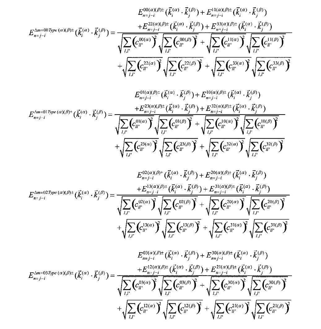
分子が自己相関となる時の例外定義は以下のようになる。
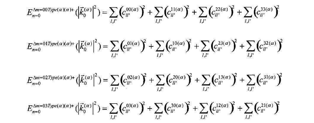
軸反転性に関して、α面とβ面のそれぞれの4つの状態に対して、展開係数が以下のように入れ替わるので、上述の定義のエネルギー分散関係は、さらに4×4倍のエネルギー分散関係が独立に定義できる。

エネルギーの要素の数は、[]が配列を表すものとすると、
[α面とβ面の組み合わせの数][Δmの型の数][α面の軸反転性の数][β面の軸反転性の数][α面の並び替え方の数][β面の並び替え方の数][対称積か反対称積かの種別][エネルギー準位数]
=6×4×4×4×12×12×2×50
となる。
エネルギーの要素の数は、[]が配列を表すものとすると、
[α面とβ面の組み合わせの数][Δmの型の数][α面の軸反転性の数][β面の軸反転性の数][α面の並び替え方の数][β面の並び替え方の数][対称積か反対称積かの種別][エネルギー準位数]
=6×4×4×4×12×12×2×50
となる。
方向組み合わせに関する平均的エネルギー分散関係への縮約については、同様の考え方が成り立つ。このときのエネルギー要素の数は、
[α面とβ面の組み合わせの数][Δmの型の数][α面の軸反転性の数][β面の軸反転性の数][エネルギー準位数]
=6×4×4×4×50
となる。
[α面とβ面の組み合わせの数][Δmの型の数][α面の軸反転性の数][β面の軸反転性の数][エネルギー準位数]
=6×4×4×4×50
となる。
[第10の実施形態]
6×6方向組み合わせで、方向組み合わせ平均によって対称積、反対称積が共に残る場合
第8の実施形態の手順8-5と第9の実施形態の手順9-5では、2次元展開係数からエネルギーの要素を作るとき、一次元配列への並び替えを12方向にとり、(α)面と(β)面の積を12×12方向の組み合わせに関してエネルギー分散関係

を導いた。しかしながら、12方向の並び替えは正の方向と負の方向の2種類をとっているので、正の方向のみの6方向の並び替えだけを選択するという考え方も存在する。
6×6方向組み合わせで、方向組み合わせ平均によって対称積、反対称積が共に残る場合
第8の実施形態の手順8-5と第9の実施形態の手順9-5では、2次元展開係数からエネルギーの要素を作るとき、一次元配列への並び替えを12方向にとり、(α)面と(β)面の積を12×12方向の組み合わせに関してエネルギー分散関係
を導いた。しかしながら、12方向の並び替えは正の方向と負の方向の2種類をとっているので、正の方向のみの6方向の並び替えだけを選択するという考え方も存在する。
第8の実施形態の手順8-5の場合だけを例に説明する。
8-5.エネルギーの要素Enの計算

は6×6通りの組み合わせのエネルギー分散関係を記述しているものとする。
8-5.エネルギーの要素Enの計算
は6×6通りの組み合わせのエネルギー分散関係を記述しているものとする。
このときのエネルギーの要素の数は、[]が配列を表すものとすると、
[α面とβ面の組み合わせの数][α面の軸反転性の数][β面の軸反転性の数][α面の並び替え方の数][β面の並び替え方の数][対称積か反対称積かの種別][エネルギー準位数]
=6×4×4×6×6×2×50
となる。
[α面とβ面の組み合わせの数][α面の軸反転性の数][β面の軸反転性の数][α面の並び替え方の数][β面の並び替え方の数][対称積か反対称積かの種別][エネルギー準位数]
=6×4×4×6×6×2×50
となる。
6×6方向組み合わせに関する平均的エネルギー分散関係を求めると、12×12方向組み合わせの場合と違って、反対称積の平均的エネルギー分散関係も残ることになる。

このときのエネルギー要素の数は、
[α面とβ面の組み合わせの数][α面の軸反転性の数][β面の軸反転性の数][対称積か反対称積かの種別][エネルギー準位数]
=6×4×4×2×50
となる。
このときのエネルギー要素の数は、
[α面とβ面の組み合わせの数][α面の軸反転性の数][β面の軸反転性の数][対称積か反対称積かの種別][エネルギー準位数]
=6×4×4×2×50
となる。
実験的に確認したところ平均的エネルギー分散関係を用いてエネルギー要素を定義した場合、第8の実施形態と第10の実施形態の特徴を捕まえる能力はほとんど同じである。
従って、どちらを使ってもよい。
従って、どちらを使ってもよい。
なお、これまでの実施形態では、周波数記述における運動量の定義を、分布関数を基底関数で展開した展開係数そのものを運動量としてきた。従って、展開係数の個数に等しい運動量の要素の数が存在していた。しかしながら、これをもっと縮約して考え、各々の部分系で色面単位で展開係数の全ての和をとった全運動量を運動量の定義とすることもできる。あるいは、展開係数の数で割っておけば、色面単位での平均運動量ということもできる。軸反転性を考慮しなければ、この場合の運動量の定義は、1つの色面から1つの運動量の要素が導出されるが、軸反転性に意味があるので要素数の数に関しては角運動量の導出で縮約される要素数と似た関係になる。
このように、全運動量で代表させた場合は、軸反転性によって、別の独立な代表値を導くことができる。一次元分布の部分系の場合は、一軸反転だけが可能なので2倍の独立要素となる。二次元分布の部分系の場合は、2軸反転が可能なのでその組み合わせから4倍の独立要素が生まれる。
このように周波数記述における運動量も平均値で記述することにすれば、実空間記述において採用した運動量が、モデル・ハミルトニアンの平均場近似の考え方から導いたのと同じく、平均値を代表値に採用させるという考え方の記述法になる。
また、上述の各実施形態によれば、
(1) 少なくとも2つの色面α,β(α=βの場合を含む)に関する画像の2次元分布関数f(α)(x,y),f(β)(x,y)の各々を入力する分布関数入力ステップと、前記2つの分布関数の各々を、x方向とy方向の各分布域内で完全系をなし互いに直交するn個の基底関数ψn(n:量子数)を用いて2次元級数展開
f(α)(x,y)=c00 (α)ψ0(y)ψ0(x)+...+c0,n-1 (α)ψ0(y)ψn-1(x)
+...
+cn-1,0 (α)ψn-1(y)ψ0(x)+...+cn-1,n-1 (α)ψn-1(y)ψn-1(x),
f(β)(x,y)=c00 (β)ψ0(y)ψ0(x)+...+c0,n-1 (β)ψ0(y)ψn-1(x)
+...
+cn-1,0 (β)ψn-1(y)ψ0(x)+...+cn-1,n-1 (β)ψn-1(y)ψn-1(x)
し、2次元展開係数cij (α),cij (β)(i=0,1,…,n-1; j=0,1,…,n-1)によって前記2つの分布関数の各々を記述する記述ステップと、前記展開係数の2次元平面において、iが増える方向を+ky方向、jが増える方向を+kx方向、iとjが同時に増える方向を+kd方向、iが増えてjが減る方向を+kd’方向、更に(i,j)=(0,0)の座標点を(kx,ky)=(0,0), (i,j)=(n-1,0)の座標点を(kx,ky)=(0,2π/a), (i,j)=(0,n-1)の座標点を(kx,ky)=(2π/a,0), (i,j)=(n-1,n-1)の座標点を(kx,ky)=(2π/a,2π/a)と定義するとき、前記2次元展開係数cij (α),cij (β)の各々を
1) (kx,ky)=(0,0)を始点とする+ky方向、
2) (kx,ky)=(0,0)を始点とする+kx方向、
3) (kx,ky)=(0,0)を始点とする+kd方向、
4) (kx,ky)=(2π/a,0)を始点とする+kd’方向、
5) (kx,ky) =(π/a,0)を始点とする+ky方向、
6) (kx,ky) =(0,π/a)を始点とする+kx方向、
7) (kx,ky) =(2π/a,2π/a)を始点とする-ky方向、
8) (kx,ky) =(2π/a,2π/a)を始点とする-kx方向、
9) (kx,ky) =(2π/a,2π/a)を始点とする-kd方向、
10) (kx,ky) =(0,2π/a)を始点とする-kd’方向、
11) (kx,ky) =(π/a,2π/a)を始点とする-ky方向、
12) (kx,ky) =(2π/a,π/a)を始点とする-kx方向
の順に12通りの一次元配列の展開係数ci (α),ci (β)(i=0,1,…,n×n-1)に並び替える並び替えステップと、前記2つの分布関数の各々12通りに並び替えられたi番目とk番目の展開係数を相互に掛け合わせることにより、対称積で表される2次形式の要素
ci (α)ck (β)+ck (α)ci (β)
を12×12通りの並び替えの方向組み合わせについてそれぞれ生成する要素生成ステップと、前記生成された144通りの2次形式の要素の各々について、一定の量子数の差m=i-kを持った全ての要素の和をとった物理量Em=i-k (α)(β)+を、複数の量子数の差に対して生成する物理量生成ステップと、前記生成された各々の物理量の少なくとも1つに基づき、前記画像の2次元分布関数の形状の特徴を評価する評価ステップと、前記評価結果に基づいて前記画像を少なくとも2つの範疇の画像に分類する分類ステップと、を備えたことを特徴とする画像分類方法、
(2) (1)に記載の画像分類方法において、前記物理量算出ステップは、物理量Em=i-k (α)(β)+をm=0,1,...,n-1のn個の量子数の差に対して生成することを特徴とする画像分類方法、
(3) (1)に記載の画像分類方法において、前記物理量生成ステップは、前記144通りの方向組み合わせについてそれぞれ生成された物理量Em=i-k (α)(β)+を、一定の量子数の差を持つもの同士の間で144通りの方向組み合わせに関して平均した物理量< Em=i-k (α)(β)+>を生成することを特徴とする画像分類方法、
(4) (1)に記載の画像分類方法において、前記要素生成ステップは更に、前記α面の2次元分布関数f(α)(x,y)の展開係数とともにy軸を反転した2次元分布関数f(α)(x,-y)=f(α’)(x,y)、x軸を反転した2次元分布関数f(α)(-x,y)=f(α’’)(x,y)、x軸とy軸を両反転した2次元分布関数f(α)(-x,-y)=f(α’’’)(x,y)の各展開係数を合わせた計4種類の場合のα面の展開係数と、前記β面の2次元分布関数f(β)(x,y)の展開係数とともにy軸を反転した2次元分布関数f(β)(x,-y)=f(β’)(x,y)、x軸を反転した2次元分布関数f(β)(-x,y)=f(β’’)(x,y)、x軸とy軸を両反転した2次元分布関数f(β)(-x,-y)=f(β’’’)(x,y)の各展開係数を合わせた計4種類の場合のβ面の展開係数についても同様に、4×4倍の2次形式の要素を生成し、 前記物理量生成ステップは軸反転に伴って増えた4×4倍の場合についても同様に、前記144通りの方向組み合わせのそれぞれについて物理量Em=i-k (α)(-β)+を生成することを特徴とする画像分類方法、
(5) 少なくとも2つの色面α,β(α=βの場合を含む)に関する画像の2次元分布関数f(α)(x,y),f(β)(x,y)の各々を入力する分布関数入力ステップと、前記2つの分布関数の各々を、x方向とy方向の各分布域内で完全系をなし互いに直交するn個の基底関数ψn(n:量子数)を用いて2次元級数展開
f(α)(x,y)=c00 (α)ψ0(y)ψ0(x)+...+c0,n-1 (α)ψ0(y)ψn-1(x)
+...
+cn-1,0 (α)ψn-1(y)ψ0(x)+...+cn-1,n-1 (α)ψn-1(y)ψn-1(x),
f(β)(x,y)=c00 (β)ψ0(y)ψ0(x)+...+c0,n-1 (β)ψ0(y)ψn-1(x)
+...
+cn-1,0 (β)ψn-1(y)ψ0(x)+...+cn-1,n-1 (β)ψn-1(y)ψn-1(x)
し、2次元展開係数cij (α),cij (β)(i=0,1,…,n-1; j=0,1,…,n-1)によって前記2つの分布関数の各々を記述する記述ステップと、前記展開係数の2次元平面において、iが増える方向を+ky方向、jが増える方向を+kx方向、iとjが同時に増える方向を+kd方向、iが増えてjが減る方向を+kd’方向、更に(i,j)=(0,0)の座標点を(kx,ky)=(0,0), (i,j)=(n-1,0)の座標点を(kx,ky)=(0,2π/a), (i,j)=(0,n-1)の座標点を(kx,ky)=(2π/a,0), (i,j)=(n-1,n-1)の座標点を(kx,ky)=(2π/a,2π/a)と定義するとき、前記2次元展開係数cij (α),cij (β)の各々を
1) (kx,ky)=(0,0)を始点とする+ky方向、
2) (kx,ky)=(0,0)を始点とする+kx方向、
3) (kx,ky)=(0,0)を始点とする+kd方向、
4) (kx,ky)=(2π/a,0)を始点とする+kd’方向、
5) (kx,ky)=(π/a,0)を始点とする+ky方向、
6) (kx,ky)=(0,π/a)を始点とする+kx方向
の順に6通りの一次元配列の展開係数ci (α),ci (β) (i=0,1,…,nxn-1)に並び替える並び替えステップと、前記2つの分布関数の各々6通りに並び替えられたi番目とk番目の展開係数を相互に掛け合わせることにより、対称積と反対称積で表される2つの型の2次形式の要素
ci (α)ck (β)+ck (α)ci (β),
ci (α)ck (β)-ck (α)ci (β)
を6×6通りの並び替えの方向組み合わせについてそれぞれ生成する要素生成ステップと、前記生成された36通りの2つの型の2次形式の要素の各々について、一定の量子数の差m=i-kを持った全ての要素の和をとった物理量Em=i-k (α)(β)+, Em=i-k (α)(β)-を、複数の量子数の差に対して生成する物理量生成ステップと、前記生成された各々の物理量の少なくとも1つに基づき、前記画像の2次元分布関数の形状の特徴を評価する評価ステップと、前記評価結果に基づいて前記画像を少なくとも2つの範疇の画像に分類する分類ステップと、を備えたことを特徴とする画像分類方法、
(6) (5)に記載の画像分類方法において、前記物理量算出ステップは、物理量Em=i-k (α)(β)+, Em=i-k (α)(β)-をm=0,1,...,n-1のn個の量子数の差に対して生成することを特徴とする画像分類方法、
(7) (5)に記載の画像分類方法において、前記物理量生成ステップは、前記36通りの方向組み合わせについてそれぞれ生成された物理量Em=i-k (α)(β)+, Em=i-k (α)(β)-を、一定の量子数の差を持つもの同士の間で36通りの方向組み合わせに関して平均した物理量<Em=i-k (α)(β)+>,<Em=i-k (α)(β)->を生成することを特徴とする画像分類方法、
(8) (5)に記載の画像分類方法において、前記要素生成ステップは更に、前記α面の2次元分布関数f(α)(x,y)の展開係数とともにy軸を反転した2次元分布関数f(α)(x,-y)= f(α’)(x,y)、x軸を反転した2次元分布関数f(α)(-x,y) = f(α’’)(x,y)、x軸とy軸を両反転した2次元分布関数f(α)(-x,-y) = f(α’’’)(x,y)の各展開係数を合わせた計4種類の場合のα面の展開係数と、前記β面の2次元分布関数f(β)(x,y)の展開係数とともにy軸を反転した2次元分布関数f(β)(x,-y) = f(β’)(x,y)、x軸を反転した2次元分布関数f(β)(-x,y) = f(β’’)(x,y)、x軸とy軸を両反転した2次元分布関数f(β)(-x,-y) = f(β’’’)(x,y)の各展開係数を合わせた計4種類の場合のβ面の展開係数についても同様に、4×4倍の2次形式の要素を生成し、前記物理量生成ステップは軸反転に伴って増えた4×4倍の場合についても同様に、前記36通りの方向組み合わせのそれぞれについて物理量Em=i-k (α)(-β)+,Em=i-k (α)(-β)-を生成することを特徴とする画像分類方法、
(9) (1)又は(5)に記載の画像分類方法において、前記評価ステップは、前記生成された各々の物理量全ての線形結合で表される、1つの線形和の物理量に基づいて、前記画像の2次元分布関数の形状の特徴を評価することを特徴とする画像分類方法、
(10) 少なくとも1つの色面αに関する画像の2次元分布関数f(α)(x,y)を入力する分布関数入力ステップと、前記分布関数を、x方向とy方向の各分布域内で完全系をなし互いに直交するn個の基底関数ψn(n:量子数)を用いて2次元級数展開
f(α)(x,y)=c00 (α)ψ0(y)ψ0(x)+...+c0,n-1 (α)ψ0(y)ψn-1(x)
+...
+cn-1,0 (α)ψn-1(y)ψ0(x)+...+cn-1,n-1 (α)ψn-1(y)ψn-1(x)
し、2次元展開係数cij (α) (i=0,1,…,n-1; j=0,1,…,n-1)によって前記分布関数を記述する記述ステップと、前記2次元展開係数cij (α)のi=jを満たす対角成分の全ての係数について、対応する基底関数の量子数iと展開係数cii (α)との積をとった対角和に相当する物理量を生成する物理量生成ステップと、前記生成された物理量に基づき、前記画像の2次元分布関数の形状の特徴を評価する評価ステップと、前記評価結果に基づいて前記画像を少なくとも2つの範疇の画像に分類する分類ステップと、を備えたことを特徴とする画像分類方法、
(11) (10)に記載の画像分類方法において、前記物理量生成ステップは更に、前記α面の2次元分布関数をy軸を反転した2次元分布関数f(α)(x,-y) = f(α’)(x,y)の2次元展開係数cij (α’)についても同様に、対角和に相当する物理量を生成することを特徴とする画像分類方法、
(12) (1)、(5)又は(10)に記載の画像分類方法において、前記分布関数入力ステップが、色面の画像の分布関数を入力するとき、前記記述ステップは、前記基底関数としてルジャンドル陪関数を用いることを特徴とする画像分類方法、
(13) (1)、(5)又は(10)に記載の画像分類方法において、前記分布関数入力ステップが、色面のエッジ成分に関するエッジ画像の分布関数を入力するとき、前記記述ステップは、前記基底関数としてフーリエ関数を用いることを特徴とする画像分類方法、
(14) (13)に記載の画像分類方法において、前記エッジ画像の分布関数は、前記画像をフィルタリングして逐次的に複数の解像度からなる高周波サブバンド画像を生成し、前記高周波サブバンド画像を低い解像度から逐次的に統合して、一つに統合されたた高周波画像を生成し、前記1つに統合された高周波画像の各画素値を2乗することによって零以上の値で定義されるエッジ面の画像の分布関数であることを特徴とする画像分類方法が提供される。
(1)~(14)記載の画像分類方法によれば、2次元分布関数を、それらの信号分布の性質に合った直交基底関数を用いて級数展開することにより、形を認識するときの均等な認識空間へ射影する周波数表現をした上で、その周波数面の係数分布の性質を展開係数の2次形式の特徴量として既約表現したことにより、最もコンパクトでスケール不変でかつ方向性に関する不変性を備えつつ、同一の感性を呼び起こす画像の間で、あるいは共通の認識を持つ物体構造が映った画像の間で保存する、同一感性の画像間の統計平均によっても消滅しない情報量に変換することを可能とした。また、これらの特徴量の相加的な性質を保証したことにより、画像の特徴量のどのような要素が心理的な印象の作用を強く呼び起こすのかについての心理構造の解明も容易にする記述が可能となった。
さらに、上述の各実施形態によれば、
(15) 少なくとも1つの色面αに関する画像A(x,y)を入力する画像入力ステップと、前記α面の画像の画素値を全ての画素値の和で規格化した分布関数f(α)(x,y)を作成する分布関数作成ステップと、前記分布関数を用いて、空間分布の重心位置(<xA>,<yA>)と、重心位置からの空間方向に関する2次モーメントの平均的な広がり幅<(y-<yA>)2>, -<(x-<xA>)(y-<yA>)>, -<(y-<yA>)(x-<xA>)>, <(x-<xA>)2> を表す慣性テンソルI11 (α),I12 (α),I21 (α),I22 (α)の各々を求めて、空間的な形状因子を記述する空間因子記述ステップと、前記α面の画像A(x,y)をy軸方向に関して画素値の平均をとってx軸に射影した一次元画像A(x)と、x軸方向に関して画素値の平均をとってy軸に射影した一次元画像A(y)とを算出する一次元画像作成ステップと、画像全体の画素値の明るさの平均値<A>を算出するとともに、x軸射影の画像A(x)を用いて前記明るさの平均値<A>から見たx軸射影の明るさの広がり幅σ1 (α)を算出し、y軸射影の画像A(y)を用いて前記明るさの平均値<A>から見たy軸射影の明るさの広がり幅σ2 (α)を算出することによって、画素値の明るさ方向の因子を記述する明るさ因子記述ステップと、前記空間因子記述ステップと前記明るさ因子記述ステップで求めた各々の量から明るさ因子に関する2次形式の物理量
(<xA>2+<yA>2)<A><A>,
I11 (α)σ1 (α)σ1 (α)+I12 (α)σ1 (α)σ2 (α)+I21 (α)σ2 (α)σ1 (α)+I22 (α)σ2 (α)σ2 (α),
I11 (α)σ1 (α)σ1 (α)+I12 (α)σ1 (α)σ2 (α)-I21 (α)σ2 (α)σ1 (α)-I22 (α)σ2 (α)σ2 (α),
I11 (α)σ1 (α)σ1 (α)-I12 (α)σ1 (α)σ2 (α)+I21 (α)σ2 (α)σ1 (α)-I22 (α)σ2 (α)σ2 (α),
I11 (α)σ1 (α)σ1 (α)-I12 (α)σ1 (α)σ2 (α)-I21 (α)σ2 (α)σ1 (α)+I22 (α)σ2 (α)σ2 (α)
の各々を算出する物理量算出ステップと、前記算出された少なくとも1つの物理量に基づいて、前記画像を少なくとも2つの範疇の画像に分類する分類ステップと、を備えたことを特徴とする画像分類方法、
(16) (15)に記載の画像分類方法において、前記物理量算出ステップは、更に前記算出された2次形式の物理量の各々の線形結合で表される1つの線形和の物理量を算出し、前記分類ステップは、前記算出された1つの線形和の物理量に基づいて、前記画像を少なくとも2つの範疇の画像に分類することを特徴とする画像分類方法、
(17) (15)に記載の画像分類方法において、前記画像入力ステップが、色面のエッジ成分に関する正負の値を持つ画像を入力するとき、前記分布関数作成ステップは、前記エッジ成分に関する画像の画素値を2乗して零以上の範囲で定義される画素値の分布に変換した上で、全ての画素値の和で規格化した分布関数を作成することを特徴とする画像分類方法、
(18) (17)に記載の画像分類方法において、前記エッジ成分に関する画像は、前記画像をフィルタリングして逐次的に複数の解像度からなる高周波サブバンド画像を生成し、前記高周波サブバンド画像を低い解像度から逐次的に統合して、一つに統合されたた高周波画像であることを特徴とする画像分類方法、
(19) 少なくとも2つの色面α,β(α≠β)に関する画像A(x,y),B(x,y)を入力する画像入力ステップと、前記α面の画像の画素値をα面の全ての画素値の和で規格化したα面の分布関数f(α)(x,y)と、前記β面の画像の画素値をβ面の全ての画素値の和で規格化したβ面の分布関数f(β)(x,y)を作成する分布関数作成ステップと、前記α面の分布関数と前記β面の分布関数の積で表された値を、全ての画素について和をとった値で規格化したα面とβ面の合成分布関数f(αβ)(x,y)を作成する合成分布関数作成ステップと、前記合成分布関数を用いて、合成色面の空間分布の重心位置(<xAB>,<yAB>)と、重心位置からの空間方向に関する2次モーメントの平均的な広がり幅<(y-<yAB>)2>, -<(x-<xAB>)(y-<yAB>)>, -<(y-<yAB>)(x-<xAB>)>, <(x-<xAB>)2> を表す慣性テンソルI11 (αβ),I12 (αβ),I21 (αβ),I22 (αβ)の各々を求めて、合成面の空間的な形状因子を記述する合成面の空間因子記述ステップと、前記α面の画像A(x,y)をy軸方向に関して画素値の平均をとってx軸に射影した一次元画像A(x)と、x軸方向に関して画素値の平均をとってy軸に射影した一次元画像A(y)とを算出するα面の一次元画像作成ステップと、前記β面の画像B(x,y)をy軸方向に関して画素値の平均をとってx軸に射影した一次元画像B(x)と、x軸方向に関して画素値の平均をとってy軸に射影した一次元画像B(y)とを算出するβ面の一次元画像作成ステップと、α面の画像全体の画素値の明るさの平均値<A>を算出するとともに、α面のx軸射影の画像A(x)を用いて前記明るさの平均値<A>から見たx軸射影の明るさの広がり幅σ1 (α)を算出し、α面のy軸射影の画像A(y)を用いて前記明るさの平均値<A>から見たy軸射影の明るさの広がり幅σ2 (α)を算出することによって、α面の画素値の明るさ方向の因子を記述するα面の明るさ因子記述ステップと、β面の画像全体の画素値の明るさの平均値<B>を算出するとともに、β面のx軸射影の画像B(x)を用いて前記明るさの平均値<B>から見たx軸射影の明るさの広がり幅σ1 (β)を算出し、β面のy軸射影の画像B(y)を用いて前記明るさの平均値<B>から見たy軸射影の明るさの広がり幅σ2 (β)を算出することによって、β面の画素値の明るさ方向の因子を記述するβ面の明るさ因子記述ステップと、前記合成面の空間因子記述ステップとα面の前記明るさ因子記述ステップとβ面の前記明るさ因子記述ステップで求めた各々の量から明るさ因子に関する2次形式の物理量
(<xAB>2+<yAB>2)<A><B>,
I11 (αβ)σ1 (α)σ1 (β)+I12 (αβ)σ1 (α)σ2 (β)+I21 (αβ)σ2 (α)σ1 (β)+I22 (αβ)σ2 (α)σ2 (β),
I11 (αβ)σ1 (α)σ1 (β)+I12 (αβ)σ1 (α)σ2 (β)-I21 (αβ)σ2 (α)σ1 (β)-I22 (αβ)σ2 (α)σ2 (β),
I11 (αβ)σ1 (α)σ1 (β)-I12 (αβ)σ1 (α)σ2 (β)+I21 (αβ)σ2 (α)σ1 (β)-I22 (αβ)σ2 (α)σ2 (β),
I11 (αβ)σ1 (α)σ1 (β)-I12 (αβ)σ1 (α)σ2 (β)-I21 (αβ)σ2 (α)σ1 (β)+I22 (αβ)σ2 (α)σ2 (β)
の各々を算出する物理量算出ステップと、前記算出された少なくとも1つの物理量に基づいて、前記画像を少なくとも2つの範疇の画像に分類する分類ステップと、を備えたことを特徴とする画像分類方法、
(20) (19)に記載の画像分類方法において、前記物理量算出ステップは、更に前記算出された2次形式の物理量の各々の線形結合で表される1つの線形和の物理量を算出し、前記分類ステップは、前記算出された1つの線形和の物理量に基づいて、前記画像を少なくとも2つの範疇の画像に分類することを特徴とする画像分類方法、
(21) (19)に記載の画像分類方法において、前記画像入力ステップが、色面のエッジ成分に関する正負の値を持つ画像を各々入力するとき、前記分布関数作成ステップは、前記エッジ成分に関する画像の画素値を2乗して零以上の範囲で定義される画素値の分布に各々変換した上で、全ての画素値の和で規格化した分布関数を各々作成することを特徴とする画像分類方法、
(22) (21)に記載の画像分類方法において、前記エッジ成分に関する画像は、前記画像をフィルタリングして逐次的に複数の解像度からなる高周波サブバンド画像を生成し、前記高周波サブバンド画像を低い解像度から逐次的に統合して、一つに統合されたた高周波画像であることを特徴とする画像分類方法、
(23) 少なくとも1つの色面αに関する画像A(x,y)を入力する画像入力ステップと、前記α面の画像の画素値を全ての画素値の和で規格化した分布関数f(α)(x,y)を作成する分布関数作成ステップと、前記分布関数を用いて、空間分布の重心位置(<xA>,<yA>)と、重心位置からの空間方向に関する2次モーメントの平均的な広がり幅<(y-<yA>)2>, -<(x-<xA>)(y-<yA>)>, -<(y-<yA>)(x-<xA>)>, <(x-<xA>)2> を表す慣性テンソルI11 (α),I12 (α),I21 (α),I22 (α)の各々を求めて、空間的な形状因子を記述する空間因子記述ステップと、前記α面の画像A(x,y)をy軸方向に関して画素値の平均をとってx軸に射影した一次元画像A(x)と、x軸方向に関して画素値の平均をとってy軸に射影した一次元画像A(y)とを算出する一次元画像作成ステップと、画像全体の画素値の明るさの平均値<A>を算出するとともに、x軸射影の画像A(x)を用いて前記明るさの平均値<A>から見たx軸射影の明るさの広がり幅σ1 (α)を算出し、y軸射影の画像A(y)を用いて前記明るさの平均値<A>から見たy軸射影の明るさの広がり幅σ2 (α)を算出することによって、画素値の明るさ方向の因子を記述する明るさ因子記述ステップと、前記空間因子記述ステップと前記明るさ因子記述ステップで求めた各々の量から明るさ因子に関する一次形式の物理量
I11 (α) σ1 (α)+ I12 (α) σ2 (α),
I21 (α) σ1 (α)+ I22 (α) σ2 (α),
I11 (α) σ1 (α)- I12 (α) σ2 (α),
I21 (α) σ1 (α)- I22 (α) σ2 (α)
の各々を算出する物理量算出ステップと、前記算出された少なくとも1つの物理量に基づいて、前記画像を少なくとも2つの範疇の画像に分類する分類ステップと、を備えたことを特徴とする画像分類方法、
(24) (23)に記載の画像分類方法において、前記物理量算出ステップは、更に前記算出された一次形式の物理量の各々の線形結合で表される1つの線形和の物理量を算出し、前記分類ステップは、前記算出された1つの線形和の物理量に基づいて、前記画像を少なくとも2つの範疇の画像に分類することを特徴とする画像分類方法、
(25) (24)に記載の画像分類方法において、前記画像入力ステップが、色面のエッジ成分に関する正負の値を持つ画像を入力するとき、前記分布関数作成ステップは、前記エッジ成分に関する画像の画素値を2乗して零以上の範囲で定義される画素値の分布に変換した上で、全ての画素値の和で規格化した分布関数を作成することを特徴とする画像分類方法、
(26) (25)に記載の画像分類方法において、前記エッジ成分に関する画像は、前記画像をフィルタリングして逐次的に複数の解像度からなる高周波サブバンド画像を生成し、前記高周波サブバンド画像を低い解像度から逐次的に統合して、一つに統合されたた高周波画像であることを特徴とする画像分類方法、
(27) (16)に記載の画像分類方法において、更に、前記分布関数f(α)(x,y)から- f(α)(x,y)log(f(α)(x,y))からなる値を、分布関数が正の値を持つ画素位置(x,y)について積分したエントロピーSを算出するとともに、前記算出された2次形式の物理量の各々を1つのベクトルにまとめて表記したときのノルムに相当する量Tを算出して、その積TSを生成し、前記物理量算出ステップは、前記算出された1つの線形和に対して、更に前記生成した積TSを線形結合したものを加えることによって、1つの線形和を算出することを特徴とする画像分類方法、
(28) (24)に記載の画像分類方法において、更に、前記分布関数f(α)(x,y)から- f(α)(x,y)log(f(α)(x,y))からなる値を、分布関数が正の値を持つ画素位置(x,y)について積分したエントロピーSを算出するとともに、前記算出された一次形式の物理量の各々を1つのベクトルにまとめて表記したときのノルムに相当する量Tを算出して、その積TSを生成し、前記物理量算出ステップは、前記算出された1つの線形和に対して、更に前記生成した積TSを線形結合したものを加えることによって、1つの線形和を算出することを特徴とする画像分類方法
が提供される。
(15)~(28)記載の画像分類方法によれば、画像の信号分布の色やエッジに関する知覚認識において、注目領域や広がりに関する性質を、物理的な描像が極めて明快な形で、共通感性や共通認識を生む画像間で統計平均をとっても消滅しない特徴量として定量的に記述することを可能にした。また、これらの特徴量の相加的な性質を保証したことにより、画像の特徴量のどのような要素が心理的な印象の作用を強く呼び起こすのかについての心理構造の解明も容易にする記述が可能となった。
Claims (6)
- 色面の画像の2次元分布関数を入力する2次元色分布関数入力ステップと、
前記色面の画像をフィルタリングして逐次的に複数の解像度からなる高周波サブバンド画像を生成し、前記高周波サブバンド画像を低い解像度から逐次的に統合して、1つに統合されたた高周波画像を生成し、前記1つに統合された高周波画像の各画素値を2乗することによって零以上の値の分布で定義されるエッジ面の画像の2次元分布関数を作成する2次元エッジ分布関数作成ステップと、
前記色面の画像の2次元分布関数を、ルジャンドル陪関数をx方向とy方向の直交基底関数とする2次元ルジャンドル級数に展開し、ルジャンドル展開係数によって前記色面の画像の2次元色分布を記述するとともに、前記エッジ面の画像の2次元分布関数を、余弦関数と正弦関数をx方向とy方向の直交基底関数とする2次元フーリエ級数に展開し、フーリエ展開係数によって前記エッジ面の画像の2次元エッジ分布を記述する記述ステップと、
前記ルジャンドル展開係数と前記フーリエ展開係数に基づき、前記色面の画像の分布の特徴を評価する評価ステップと、
前記評価結果に基づいて前記色面の画像を少なくとも2つの範疇の画像に分類する分類ステップと、
を備えたことを特徴とする画像分類方法。 - 請求項1に記載の画像分類方法において、
更に、前記1つに統合された高周波画像を用いて、エッジ強度の値に関する一次元分布関数を作成する一次元エッジ分布関数作成ステップと、
前記エッジ強度に関する一次元分布関数を、球ベッセル関数を直交基底関数とする球ベッセル級数に展開し、球ベッセル展開係数によって前記エッジ強度の一次元分布を記述する記述ステップとを備え、
前記評価ステップは、前記ルジャンドル展開係数と前記フーリエ展開係数に合わせて、前記球ベッセル展開係数も用いて前記色面の画像の分布の特徴を評価することを特徴とする画像分類方法。 - 請求項2に記載の画像分類方法において、
更に、前記色面の画像を用いて、画素値に関する一次元分布関数を作成する一次元色分布関数作成ステップと、
前記画素値に関する一次元分布関数を、チェビシェフ関数を直交基底関数とするチェビシェフ級数に展開し、チェビシェフ展開係数によって前記画素値の一次元分布を記述する記述ステップとを備え、
前記評価ステップは、前記ルジャンドル展開係数と前記フーリエ展開係数、前記球ベッセル展開係数に合わせて、前記チェビシェフ展開係数も用いて前記色面の画像の分布の特徴を評価することを特徴とする画像分類方法。 - 請求項1に記載の画像分類方法において、
前記評価ステップは、前記ルジャンドル展開係数から該展開係数の2次形式で表される特徴量と、前記フーリエ展開係数から該展開係数の2次形式で表される特徴量とを生成し、更にこれらの特徴量の線形和で表される1つの特徴量を生成し、前記線形和で表された1つの特徴量に基づいて前記色面の画像の分布の特徴を評価することを特徴とする画像分類方法。 - 請求項2に記載の画像分類方法において、
前記評価ステップは、前記ルジャンドル展開係数から該展開係数の2次形式で表される特徴量と、前記フーリエ展開係数から該展開係数の2次形式で表される特徴量と、前記球ベッセル展開係数から該展開係数の2次形式で表される特徴量とを生成し、更にこれらの特徴量の線形和で表される1つの特徴量を生成し、前記線形和で表された1つの特徴量に基づいて前記色面の画像の分布の特徴を評価することを特徴とする画像分類方法。 - 請求項3に記載の画像分類方法において、
前記評価ステップは、前記ルジャンドル展開係数から該展開係数の2次形式で表される特徴量と、前記フーリエ展開係数から該展開係数の2次形式で表される特徴量と、前記球ベッセル展開係数から該展開係数の2次形式で表される特徴量と、前記球チェビシェフ展開係数から該展開係数の2次形式で表される特徴量とを生成し、更にこれらの特徴量の線形和で表される1つの特徴量を生成し、前記線形和で表された1つの特徴量に基づいて前記色面の画像の分布の特徴を評価することを特徴とする画像分類方法。
Priority Applications (2)
| Application Number | Priority Date | Filing Date | Title |
|---|---|---|---|
| CN201280030264.0A CN103620647A (zh) | 2011-07-08 | 2012-06-12 | 图像分类方法 |
| US14/130,188 US20140348423A1 (en) | 2011-07-08 | 2012-06-12 | Image sorting method |
Applications Claiming Priority (2)
| Application Number | Priority Date | Filing Date | Title |
|---|---|---|---|
| JP2011-151622 | 2011-07-08 | ||
| JP2011151622A JP2013020335A (ja) | 2011-07-08 | 2011-07-08 | 画像分類方法 |
Publications (1)
| Publication Number | Publication Date |
|---|---|
| WO2013008573A1 true WO2013008573A1 (ja) | 2013-01-17 |
Family
ID=47505871
Family Applications (1)
| Application Number | Title | Priority Date | Filing Date |
|---|---|---|---|
| PCT/JP2012/064975 Ceased WO2013008573A1 (ja) | 2011-07-08 | 2012-06-12 | 画像分類方法 |
Country Status (4)
| Country | Link |
|---|---|
| US (1) | US20140348423A1 (ja) |
| JP (1) | JP2013020335A (ja) |
| CN (1) | CN103620647A (ja) |
| WO (1) | WO2013008573A1 (ja) |
Cited By (1)
| Publication number | Priority date | Publication date | Assignee | Title |
|---|---|---|---|---|
| WO2024018590A1 (ja) * | 2022-07-21 | 2024-01-25 | 日本電信電話株式会社 | 主観補正装置、主観補正方法及び主観補正プログラム |
Families Citing this family (24)
| Publication number | Priority date | Publication date | Assignee | Title |
|---|---|---|---|---|
| US11080318B2 (en) * | 2013-06-27 | 2021-08-03 | Kodak Alaris Inc. | Method for ranking and selecting events in media collections |
| JP6242098B2 (ja) * | 2013-07-16 | 2017-12-06 | 株式会社キーエンス | 三次元画像処理装置、三次元画像処理方法及び三次元画像処理プログラム並びにコンピュータで読み取り可能な記録媒体及び記録した機器 |
| US10120879B2 (en) * | 2013-11-29 | 2018-11-06 | Canon Kabushiki Kaisha | Scalable attribute-driven image retrieval and re-ranking |
| KR20160017954A (ko) * | 2014-08-07 | 2016-02-17 | 삼성전자주식회사 | 전자장치 및 전자장치의 전송 제어 방법 |
| CN104486608B (zh) * | 2014-12-31 | 2016-07-20 | 深圳市华星光电技术有限公司 | 图像数据处理方法及装置 |
| CN105426543A (zh) * | 2015-12-28 | 2016-03-23 | 辽宁师范大学 | 基于贝塞尔统计模型的图像检索方法 |
| CN106503143B (zh) * | 2016-10-21 | 2020-02-07 | 广东工业大学 | 一种图像检索方法及装置 |
| CN108206910B (zh) * | 2016-12-20 | 2021-04-06 | 北京小米移动软件有限公司 | 图像拍摄的方法及装置 |
| CN107657037A (zh) * | 2017-09-29 | 2018-02-02 | 郑州云海信息技术有限公司 | 一种高效图像检索方法 |
| CN108986180B (zh) * | 2018-06-07 | 2022-09-16 | 创新先进技术有限公司 | 一种调色板的生成方法、装置及电子设备 |
| CN110136146B (zh) * | 2019-05-17 | 2021-01-08 | 浙江理工大学 | 基于正弦spf分布和水平集模型的sar图像水域分割方法 |
| JP7403253B2 (ja) * | 2019-07-19 | 2023-12-22 | Lineヤフー株式会社 | 学習装置、学習方法および学習プログラム |
| CN110955830B (zh) * | 2019-11-22 | 2021-02-19 | 拉扎斯网络科技(上海)有限公司 | 信息处理方法、装置、电子设备及计算机可读存储介质 |
| CN111175318A (zh) * | 2020-01-21 | 2020-05-19 | 上海悦易网络信息技术有限公司 | 屏幕划痕碎裂检测方法及设备 |
| CN111426648B (zh) * | 2020-03-19 | 2023-04-07 | 甘肃省交通规划勘察设计院股份有限公司 | 一种红外谱图的相似度确定方法及系统 |
| CN111526371B (zh) * | 2020-04-30 | 2022-12-06 | 华侨大学 | 一种基于Gabor特征和灰度共生矩阵的视频帧内编码快速算法 |
| WO2022130498A1 (ja) * | 2020-12-15 | 2022-06-23 | 三菱電機株式会社 | 類似度算出装置、類似度算出方法、及び、類似度算出プログラム |
| US11849469B2 (en) | 2021-06-18 | 2023-12-19 | Qualcomm Incorporated | Orbital angular momentum capability in millimeter wave and higher frequency bands |
| US11757516B2 (en) | 2021-06-18 | 2023-09-12 | Qualcomm Incorporated | Beam management procedure for OAM in MMW and higher bands |
| US11616555B2 (en) * | 2021-06-18 | 2023-03-28 | Qualcomm Incorporated | Spatial misalignment tracking for orbital angular momentum beams in millimeter wave and higher frequency bands |
| US12231912B2 (en) | 2021-06-18 | 2025-02-18 | Qualcomm Incorporated | System and method for reporting orbital angular momentum waveform misalignment |
| CN116360603A (zh) * | 2023-05-29 | 2023-06-30 | 中数元宇数字科技(上海)有限公司 | 基于时序信号匹配的交互方法、设备、介质及程序产品 |
| CN116577061B (zh) * | 2023-07-14 | 2023-09-15 | 常州市建筑科学研究院集团股份有限公司 | 金属屋面抗风性能的检测方法、计算机设备及介质 |
| CN117746000B (zh) * | 2023-12-27 | 2024-09-27 | 广东瑞永密封制品有限公司 | 橡胶密封圈多类表面缺陷分类定位方法 |
Citations (3)
| Publication number | Priority date | Publication date | Assignee | Title |
|---|---|---|---|---|
| JP2010072699A (ja) * | 2008-09-16 | 2010-04-02 | Nikon Corp | 画像分類装置および画像処理装置 |
| JP2011040050A (ja) * | 2009-07-15 | 2011-02-24 | Nikon Corp | 画像分類装置 |
| JP2011040049A (ja) * | 2009-07-15 | 2011-02-24 | Nikon Corp | 画像分類装置 |
Family Cites Families (8)
| Publication number | Priority date | Publication date | Assignee | Title |
|---|---|---|---|---|
| JP3708621B2 (ja) * | 1996-04-15 | 2005-10-19 | 富士写真フイルム株式会社 | 画像読み取り装置 |
| JP3031613B2 (ja) * | 1996-11-12 | 2000-04-10 | 株式会社つくばソフト研究所 | カラー/濃淡画像入力出力装置と入力出力方法 |
| US7457435B2 (en) * | 2004-11-17 | 2008-11-25 | Euclid Discoveries, Llc | Apparatus and method for processing video data |
| US7457472B2 (en) * | 2005-03-31 | 2008-11-25 | Euclid Discoveries, Llc | Apparatus and method for processing video data |
| US7436981B2 (en) * | 2005-01-28 | 2008-10-14 | Euclid Discoveries, Llc | Apparatus and method for processing video data |
| US8600149B2 (en) * | 2008-08-25 | 2013-12-03 | Telesecurity Sciences, Inc. | Method and system for electronic inspection of baggage and cargo |
| JP4840426B2 (ja) * | 2008-09-24 | 2011-12-21 | ソニー株式会社 | 電子機器、ぼけ画像選別方法及びプログラム |
| US8478053B2 (en) * | 2009-07-15 | 2013-07-02 | Nikon Corporation | Image sorting apparatus |
-
2011
- 2011-07-08 JP JP2011151622A patent/JP2013020335A/ja not_active Withdrawn
-
2012
- 2012-06-12 CN CN201280030264.0A patent/CN103620647A/zh active Pending
- 2012-06-12 US US14/130,188 patent/US20140348423A1/en not_active Abandoned
- 2012-06-12 WO PCT/JP2012/064975 patent/WO2013008573A1/ja not_active Ceased
Patent Citations (3)
| Publication number | Priority date | Publication date | Assignee | Title |
|---|---|---|---|---|
| JP2010072699A (ja) * | 2008-09-16 | 2010-04-02 | Nikon Corp | 画像分類装置および画像処理装置 |
| JP2011040050A (ja) * | 2009-07-15 | 2011-02-24 | Nikon Corp | 画像分類装置 |
| JP2011040049A (ja) * | 2009-07-15 | 2011-02-24 | Nikon Corp | 画像分類装置 |
Non-Patent Citations (1)
| Title |
|---|
| YAP P.-T.: "Content-based image retrieval using Legendre chromaticity distribution moments", IEE PROCEEDINGS ON VISION, IMAGE AND SIGNAL PROCESSING, vol. 153, no. ISS.1, 9 February 2006 (2006-02-09), pages 17 - 24 * |
Cited By (1)
| Publication number | Priority date | Publication date | Assignee | Title |
|---|---|---|---|---|
| WO2024018590A1 (ja) * | 2022-07-21 | 2024-01-25 | 日本電信電話株式会社 | 主観補正装置、主観補正方法及び主観補正プログラム |
Also Published As
| Publication number | Publication date |
|---|---|
| US20140348423A1 (en) | 2014-11-27 |
| JP2013020335A (ja) | 2013-01-31 |
| CN103620647A (zh) | 2014-03-05 |
Similar Documents
| Publication | Publication Date | Title |
|---|---|---|
| JP2013020335A (ja) | 画像分類方法 | |
| US8478053B2 (en) | Image sorting apparatus | |
| Wolter et al. | Wavelet-packets for deepfake image analysis and detection | |
| Li et al. | Learning disentangled feature representation for hybrid-distorted image restoration | |
| JP5041041B2 (ja) | 画像分類装置 | |
| Saydjari et al. | Classification of magnetohydrodynamic simulations using wavelet scattering transforms | |
| Khosla et al. | Evaluation of Euclidean and Manhanttan metrics in content based image retrieval system | |
| Hu et al. | Decouple the object: Component-level semantic recognizer for point clouds classification | |
| Gong et al. | C3NN: cosmological correlator convolutional neural network an interpretable machine-learning framework for cosmological analyses | |
| JP2013020336A (ja) | 画像分類方法 | |
| JP5007758B2 (ja) | 画像分類装置 | |
| JP5041040B2 (ja) | 画像分類装置 | |
| JP2013020337A (ja) | 画像分類方法 | |
| JP5007757B2 (ja) | 画像分類装置 | |
| Bespalov and et al. | Scale-space representation and classification of 3d models | |
| Ignatowicz et al. | Evaluation and comparison of emotionally evocative image augmentation methods | |
| Xue et al. | Investigation of the role of aesthetics in differentiating between photographs taken by amateur and professional photographers | |
| San-Martin-Jimenez et al. | Depthwise convolutional neural network for multiband automatic quasars classification in ATLAS | |
| Singhal et al. | Photozilla: An image dataset of photography styles and its application to visual embedding and style detection | |
| Patria et al. | A Comparative Study of MobileNetV2 and ResNet50 for Multi-Class AI-Generated and Real Image Classification | |
| Guan et al. | Spectral images and features co-clustering with application to content-based image retrieval | |
| Han et al. | Explainable interactive projections for image data | |
| Li et al. | Kernel-based spectral color image segmentation | |
| Shi et al. | Image two-classification algorithm based on continuous-time quantum walk | |
| Landre´ et al. | Automatic building of a visual interface for content-based multiresolution retrieval of paleontology images |
Legal Events
| Date | Code | Title | Description |
|---|---|---|---|
| 121 | Ep: the epo has been informed by wipo that ep was designated in this application |
Ref document number: 12811777 Country of ref document: EP Kind code of ref document: A1 |
|
| NENP | Non-entry into the national phase |
Ref country code: DE |
|
| WWE | Wipo information: entry into national phase |
Ref document number: 14130188 Country of ref document: US |
|
| 122 | Ep: pct application non-entry in european phase |
Ref document number: 12811777 Country of ref document: EP Kind code of ref document: A1 |