WO2006057359A1 - 直交基底気泡関数要素数値解析方法、直交基底気泡関数要素数値解析プログラムおよび直交基底気泡関数要素数値解析装置 - Google Patents
直交基底気泡関数要素数値解析方法、直交基底気泡関数要素数値解析プログラムおよび直交基底気泡関数要素数値解析装置 Download PDFInfo
- Publication number
- WO2006057359A1 WO2006057359A1 PCT/JP2005/021727 JP2005021727W WO2006057359A1 WO 2006057359 A1 WO2006057359 A1 WO 2006057359A1 JP 2005021727 W JP2005021727 W JP 2005021727W WO 2006057359 A1 WO2006057359 A1 WO 2006057359A1
- Authority
- WO
- WIPO (PCT)
- Prior art keywords
- equation
- analysis
- bubble function
- mass matrix
- matrix
- Prior art date
- Legal status (The legal status is an assumption and is not a legal conclusion. Google has not performed a legal analysis and makes no representation as to the accuracy of the status listed.)
- Ceased
Links
Classifications
-
- G—PHYSICS
- G06—COMPUTING OR CALCULATING; COUNTING
- G06F—ELECTRIC DIGITAL DATA PROCESSING
- G06F30/00—Computer-aided design [CAD]
- G06F30/20—Design optimisation, verification or simulation
- G06F30/23—Design optimisation, verification or simulation using finite element methods [FEM] or finite difference methods [FDM]
-
- G—PHYSICS
- G06—COMPUTING OR CALCULATING; COUNTING
- G06F—ELECTRIC DIGITAL DATA PROCESSING
- G06F2111/00—Details relating to CAD techniques
- G06F2111/10—Numerical modelling
Definitions
- Orthogonal basis bubble function element numerical analysis method orthogonal basis bubble function element numerical solution prayer program and orthogonal basis bubble function element numerical analysis device
- the present invention provides a highly reliable numerical simulation using a mass matrix that has only a diagonal term with high computational efficiency for analysis by a finite element method using a bubble function element (finite element analysis).
- the present invention relates to an orthogonal basis bubble function element numerical analysis method, an orthogonal basis bubble function element numerical analysis program, and an orthogonal basis bubble function element numerical analysis apparatus.
- FIG. 47 is an explanatory diagram showing a conventional two-dimensional bubble function element
- FIG. 48 is an explanatory diagram showing a conventional three-dimensional bubble function element.
- the bubble function element using a triangle (tetrahedron) element consists of 3 (4) points that form a triangle (tetrahedron) in each element and 4 (5) nodes of the center of gravity.
- the isoparametric coordinate system [r, S ] ( ⁇ r, s, t ⁇ ) for example, Non-Patent Document 1, Non-Patent Document 2, Non-Patent Reference 3).
- Equation (1) ⁇ ⁇ , ⁇ are the shape functions of the bubble function elements, and u a, u are the apexes of the triangle (tetrahedron).
- the value of the point (analysis physical quantity), the value of the center of gravity (analysis physical quantity), and N represents the number of spatial dimensions. If described in the vector format, the shape function is expressed by the following equations (3) to (6).
- ⁇ a in equation (2) is a shape function using a two-dimensional and three-dimensional primary element.
- ⁇ is called the bubble function.
- the bubble function is defined for each element so that its value ⁇ on the element boundary is 1 and the value is 1 at the center of gravity.
- the finite element equation using the bubble function element for discretization in the spatial direction can be expressed as the following equation (9).
- Equation (9) u is the unknown physical quantity to be obtained (contaminant concentration, temperature, flow rate, water depth, flow velocity, pressure, displacement, etc.), M is the mass matrix, and F (u) is other than the time derivative term This is a summarizing term.
- Equation (10) a four-stage solution based on the Tiller expansion is expressed as Equation (10) to Equation (13) below (for example, see Non-Patent Document 4 below).
- Equation (10) to Equation (13) represents the known analysis physical quantity at the current time n
- n + 1 represents the unknown analysis physical quantity after a lapse of a minute time ⁇ t from time n.
- Non-Patent Document 1 DNArnold, F. Brezzi and M. Fortin, "A Stable Finite Element for the Stokes Equations", Calcolo, Vol.23, 1984, pp.337— pp.344 (Di ⁇ ⁇ ⁇ J. Arnold, F. Brizi, and M. Fortin, “Assurable Huaynite Element for the Stusts Equisions” Chalkoguchi 23 ⁇ 1984 pp. 337 p. 344)
- Special Reference 2 J. ; mo, F. Armero and A.
- Non-Patent Document 3 Junichi Matsumoto, “Two Levels for Incompressible Viscous Flow Analysis Using Bubble Functions” "Bell-3 Level Finite Element Method", Journal of Applied Mechanics (Japan Society of Civil Engineers), 7 ⁇ , August 2004, 339—3 46
- Non-Patent Literature 4 Katsunori Hatanaka, “Computational Mechanics Study on Forward / Inverse Analysis of Incompressible Viscous Fluids by Multistage Finite Element Method”, Chuo University Doctoral Dissertation, March 1993
- Fig. 49 is an explanatory diagram showing the analysis model used for the analysis of the conventional Rotating Cone problem.
- Fig. 50 is an explanatory diagram showing the contour lines of the initial conditions used for the analysis of the conventional Rotating Cone problem.
- FIG. 10 is an explanatory diagram showing contour lines of an analysis result of a Rotating Cone problem calculated by a conventional matched mass matrix (see Non-Patent Document 4).
- the analysis model 4900 in Fig. 49 is assumed to be in an initial state (at 0 lap). Then, by using the inverse matrix of the mass matrix and rotating it from the initial state (0 lap) for a predetermined lap, for example, 5 laps, the contour model 5000 in the initial state of the analytical model 4900 shown in FIG.
- the analysis results are as shown in Fig. 1.
- the above-described mass matrix is generally a sparse distribution matrix (matched mass matrix) because it uses bubble function elements for discretization in the time direction. Therefore, obtaining the inverse matrix of this distribution matrix (consistent mass matrix) requires a large amount of storage capacity and calculation time for numerical analysis, which increases the cost of the device itself and delays the analysis process. there were.
- an approximate matrix (concentrated mass matrix) is usually used that adds the components in each row of the mass matrix (concentrates) and has the components only in the diagonal terms. Is done.
- the inverse matrix is a matrix with each diagonal component being an inverse number. Compared to the case of using a matrix, the analysis can be executed with very little storage capacity and calculation time.
- the concentrated mass matrix is not the same matrix as the original mass matrix but an approximate matrix. Therefore, when the analysis model 4900 shown in FIG. 49 is rotated from the initial state (0 lap) for a predetermined lap, for example, 5 laps, the contour model 5000 in the initial state of the analysis model 4900 shown in FIG.
- the analysis results are as shown in Fig. 52. In this way, the contour model 5200 after five revolutions of the analysis model 4900 is significantly deformed compared to the contour model 5000 in the initial state and the contour model 5100 shown in Fig. 51. There was a problem that the reliability of the results was low.
- the present invention eliminates the problems caused by the prior art described above, and an orthogonal basis bubble function element numerical analysis method and orthogonal basis bubble function element numerical analysis capable of realizing a simple and reliable finite element analysis. It is an object of the present invention to provide a program and an apparatus for numerical analysis of orthogonal basis bubble function elements.
- the orthogonal basis bubble function element numerical analysis method, the orthogonal basis bubble function element numerical analysis program, and the orthogonal basis bubble function element numerical analysis apparatus of the present invention are provided as follows:
- the matching mass matrix of each element to be analyzed was acquired, and the matching mass matrix of each element acquired by the second acquisition step was diagonalized based on the bubble function of each element to be analyzed.
- a diagonal mass matrix of each element is generated, and the behavior of the analysis target is analyzed based on the known analysis physical quantity of the analysis target and the generated diagonal mass matrix of each element.
- the diagonal mass matrix of each element may be generated by substituting the integral value of the bubble function in each element into the matched mass matrix of each element. Further, based on the generated diagonal mass matrix of the element, a diagonal mass matrix of the entire analysis target is calculated, an inverse matrix of the diagonal mass matrix of the entire analysis target is calculated, and the known analysis of the analysis target is calculated. The behavior of the analysis target may be analyzed based on the physical quantity, the diagonal mass matrix of the entire analysis target, and the inverse matrix.
- the bubble function satisfying the following conditional expression (14) in which the mass matrix is a diagonal matrix is used without performing the approximation of the mass matrix in the finite element analysis using the bubble function element.
- orthogonal basal bubble function element numerical analysis method According to the orthogonal basal bubble function element numerical analysis method, orthogonal basal bubble function element numerical analysis program, and orthogonal basal bubble function element numerical analysis device that are useful in the present invention, analysis processing is performed easily and with high accuracy. As a result, the reliability of the behavior analysis of the analysis target can be improved. In addition, if an efficient analysis method (orthogonal basal bubble function element numerical analysis method), such as a reduction in storage capacity and a reduction in analysis time, can be realized!
- FIG. 1 is a block diagram showing a hardware configuration of a numerical analysis apparatus that is useful for an embodiment of the present invention.
- FIG. 2 is a block diagram showing a functional configuration of a numerical analysis device according to an embodiment of the present invention.
- FIG. 3 is an explanatory diagram showing an analysis physical quantity information table stored in the data storage unit of the numerical analysis apparatus according to the embodiment of the present invention.
- FIG. 4 is a flowchart showing a numerical analysis processing procedure in the numerical analysis apparatus according to the embodiment of the present invention.
- FIG. 5 is an explanatory view showing a two-dimensional bubble function element.
- FIG. 6 is an explanatory view showing a three-dimensional bubble function element.
- FIG. 7 is an explanatory diagram showing a shape ⁇ of a triangular bubble function forming an orthogonal basis.
- FIG. 8 is an explanatory view showing a shape ⁇ 2 of a triangular bubble function forming an orthogonal basis.
- FIG. 9 is an explanatory diagram showing the shape ⁇ of the triangular bubble function forming the orthogonal basis.
- FIG. 10 is an explanatory diagram showing a triangular bubble function shape ⁇ 2 forming an orthogonal basis.
- FIG. 11 is an explanatory diagram showing a two-dimensional bubble function.
- FIG. 12 is an explanatory diagram showing a three-dimensional bubble function.
- FIG. 13 is an explanatory diagram showing a calculation area in the analysis of the Rotating Cone problem.
- FIG. 14 is an explanatory diagram showing an analysis model mesh in the analysis of the Rotating Cone problem.
- FIG. 15 is an explanatory diagram showing the flow velocity (flow state) of the analysis model in the analysis of the Rotating Cone problem.
- FIG. 16 is a bird's-eye view showing initial conditions in the analysis of the Rotating Cone problem.
- FIG. 17 is an explanatory diagram showing contour lines of initial conditions in the analysis of the Rotating Cone problem.
- FIG. 18 is a bird's eye view showing the calculation result using the matched mass matrix with the bubble function (Equation (47)).
- FIG. 19 is an explanatory diagram showing the contour lines of the calculation results using the matched mass matrix with the bubble function (Equation (47)).
- FIG. 20 is a bird's-eye view showing the calculation result using the concentrated mass matrix in the bubble function equation ((47)).
- Figure 21 shows the contour of the calculation result using the concentrated mass matrix with the bubble function (Equation (47)). It is explanatory drawing which shows a line.
- FIG. 22 is a bird's-eye view showing a calculation result using a matched mass matrix with a bubble function (equation (48)).
- FIG. 23 is an explanatory diagram showing contour lines of a calculation result using a matched mass matrix with a bubble function (equation (48)).
- FIG. 24 is a bird's-eye view showing a calculation result using a concentrated mass matrix with a bubble function (equation (48)).
- FIG. 25 is an explanatory diagram showing contour lines of a calculation result using a concentrated mass matrix with a bubble function (equation (48)).
- FIG. 26 is a bird's eye view showing a calculation result using a diagonal mass matrix with a bubble function (equation (49)).
- FIG. 27 is an explanatory diagram showing contour lines of a calculation result using a diagonal mass matrix with a bubble function (equation (49)).
- FIG. 28 is an explanatory diagram showing an analysis model mesh (number of nodes: 4 38 413, number of elements: 2539200) in the analysis of the Rotating Cone problem.
- FIG. 41 is an explanatory diagram (part 1) illustrating an isoparametric coordinate system r.
- FIG. 42 is an explanatory diagram (part 2) illustrating the isoparametric coordinate system r.
- FIG. 43 is an explanatory diagram showing the shape ⁇ of the triangular bubble function using equations (81) and (93).
- FIG 44 is a formula (81), an explanatory view showing the shape phi 2 triangular bubble function using (93)
- FIG. 45 is an explanatory diagram showing a shape of a triangular three-level bubble function using the equation (132).
- FIG. 46 shows a triangular bubble function using equations (81) and (93) and a triangle using equation (132).
- FIG. 47 is an explanatory view showing a conventional two-dimensional bubble function element.
- FIG. 48 is an explanatory view showing a conventional three-dimensional bubble function element.
- FIG. 49 is an explanatory diagram showing an analysis model used for analysis of a conventional Rotating Cone problem.
- FIG. 50 is an explanatory diagram showing contour lines of initial conditions used for analysis of a conventional Rotating Cone problem.
- Figure 51 shows the analysis of the Rotating Cone problem calculated by the conventional matched mass matrix. It is explanatory drawing which shows the contour line of a result.
- FIG. 52 is an explanatory diagram showing the contour lines of the analysis result of the Rotating Cone problem calculated by the conventional concentrated mass matrix.
- FIG. 1 is a block diagram showing a hardware configuration of a numerical analysis apparatus that is useful for an embodiment of the present invention.
- An FD (flexible disk) 107, a display 108, an IZF (interface) 109, a keyboard 110, a mouse 111, a scanner 112, and a printer 113 are provided.
- Each component is connected by a bus 100.
- the CPU 101 governs overall control of the numerical analysis device.
- the ROM 102 considers programs such as a boot program.
- RAM103 is the work area of CPU101 Used.
- the HDD 104 controls data read / write to the HD 105 according to the control of the CPU 101.
- the HD 105 performs data written under the control of the HDD 104. .
- the FDD 106 controls the read Z write of data to the FD 107 according to the control of the CPU 101.
- the FD 107 stores data written under the control of the FDD 106, and causes the numerical analysis device to read data stored in the FD 107.
- the power of FD107 CD-ROM (CD-R, CD-RW), MO, DVD (Digital Versatile Disk), memory card, etc. may be used.
- the display 108 displays data such as a document, an image, and function information as well as a cursor, an icon, or a tool box.
- a CRT, a TFT liquid crystal display, a plasma display or the like can be adopted.
- the IZF 109 is connected to a network such as the Internet through a communication line, and is connected to other devices via this network.
- the IZF 109 controls a network and an internal interface, and controls data input / output from an external device.
- a modem or a LAN adapter can be used as the IZF 109.
- the keyboard 110 includes keys for inputting characters, numbers, various instructions, and the like, and inputs data. Alternatively, a touch panel type input pad or a numeric keypad may be used.
- the mouse 111 is used to move the cursor, select a range, or move and change the size of windows. A track ball or a joystick may be used as long as they have the same function as a pointing device.
- the scanner 112 optically reads an image and takes in the image data into the numerical analysis device.
- the printer 113 prints image data and document data.
- a laser printer or an ink jet printer can be adopted.
- FIG. 2 is a block diagram showing a functional configuration of a numerical analysis apparatus that is useful in the embodiment of the present invention.
- the numerical analysis device 200 includes a data storage unit 201, a first acquisition unit 202, a second acquisition unit 203, a generation unit 204, a first calculation unit 205, 2 calculation unit 206 and The analysis unit 207 and the force are configured.
- the data storage unit 201 has an analysis physical quantity information table used for numerical analysis of an analysis target.
- the analysis physical quantity information table will be described.
- FIG. 3 is an explanatory diagram showing an analysis physical quantity information table that is useful for the embodiment of the present invention.
- the analysis physical quantity information table stores the analysis physical quantity ID, the analysis physical quantity name (contaminant, heat, fluid, structure, etc.), and the known analysis physical quantity for the analysis target. . Further, as the known analysis physical quantity, a known physical property value, a boundary analysis physical quantity, and an initial analysis physical quantity are stored.
- the analysis physical quantity ID and the analysis physical quantity name are information specified by a user input operation.
- the analysis physical quantity ID and the analysis physical quantity name are specified, the associated physical property value, boundary analysis physical quantity, and An initial analysis physical quantity can be extracted.
- the known physical property value is information for determining what kind of substance is the analysis target for which the analysis physical quantity ID or the analysis physical quantity name is designated by the user input operation.
- Examples of known physical property values include diffusion coefficient, density, specific heat, heat conduction coefficient, viscosity coefficient, water bottom friction coefficient, Young's modulus, Poisson's ratio, and the like.
- the boundary analysis physical quantity represents the analysis conditions under which the analysis region (mesh divided into triangles and tetrahedrons) consisting of each element to be analyzed is analyzed! Information.
- Examples of physical quantities for boundary analysis include substance concentration, temperature, flow velocity, pressure, flow rate, water depth, and displacement.
- an initial analysis physical quantity as an initial condition is further required.
- the initial analysis physical quantity is the value of the analysis physical quantity at the start of analysis.
- information such as the time increment and the number of calculation steps are also stored in the analysis physical quantity information table in order to perform sequential analysis calculation in the time direction.
- mesh information such as the division width, the number of nodes, the number of elements, the node coordinate value corresponding to the node number, and the element combination information corresponding to the element number are also stored.
- This mesh is a triangular element when the analysis target range is a two-dimensional space, and a tetrahedral element when the analysis target range is a three-dimensional space.
- the mesh can also be captured by reading it with the scanner 112 shown in FIG.
- the data storage unit 201 realizes its function by, for example, the RAM 103, HD 105, or FD 107 shown in FIG.
- the first acquisition unit 202 acquires a known analysis physical quantity to be analyzed. Specifically, by operating the input device (for example, the keyboard 110 or the mouse 111 shown in FIG. 1), the analysis physical quantity ID of the physical quantity to be analyzed is selected, and the known analysis physical quantity is extracted from the data storage unit 201. . Specifically, the first acquisition unit 202 is executed by the CPU 101 executing a program stored in the ROM 102, the RAM 103, the HD 105, the FD 107, or the like shown in FIG. 1, or by the IZF 109 shown in FIG. Realize its function.
- the second acquisition unit 203 acquires the matched mass matrix of each element (mesh) to be analyzed.
- the second acquisition unit 203 executes the program stored in the ROM 102, RAM 103, HD 105, FD 107, etc. shown in FIG. 1 by the CPU 101, or by the IZF 109 shown in FIG. Realize the function.
- the generation unit 204 diagonalizes the matched mass matrix of each element acquired by the second acquisition unit 203 based on the bubble function of each element to be analyzed. Generate a matrix. Specifically, the generation unit 204 realizes its function by, for example, the CPU 101 executing a program stored in the ROM 102, RAM 103, HD 105, FD 107, etc. shown in FIG. 1, and by the IZF 109 shown in FIG. To do.
- the first calculation unit 205 calculates a diagonal mass matrix for the entire analysis target based on the diagonal mass matrix of each element generated by the generation unit 204. Specifically, for example, the first calculation unit 205 is executed by the CPU 101 executing a program stored in the ROM 102, RAM 103, HD 105, FD 107, or the like shown in FIG. 1, or in the IZF 109 shown in FIG. Yo The function is realized.
- the second calculation unit 206 calculates the inverse matrix of the diagonal mass matrix calculated by the first calculation unit 205 over the entire area to be analyzed. Specifically, the second calculation unit 206 is executed by, for example, the CPU 101 executing the program stored in the ROM 102, RAM 103, HD 105, FD 107, etc. shown in FIG. 1, or by the IZF 109 shown in FIG. This function is realized.
- the analysis unit 207 analyzes the behavior of the analysis target based on the known analysis physical quantity acquired by the first acquisition unit 202 and the diagonal mass matrix of each element generated by the generation unit 2004. To do. Specifically, the known analysis physical quantity acquired by the first acquisition unit 202, the diagonal mass matrix of the entire analysis target calculated by the first calculation unit 205, and the second calculation unit 206 Based on the inverse matrix, the behavior of the analysis target is analyzed. There is a solution that does not require a diagonal mass matrix for the entire analysis target, but analyzes the behavior of the analysis target using only the diagonal mass matrix of each element (for example, OCZienkiewicz, R ⁇ . Tay lor, bJSherwin and J.
- the generator 204 and the first calculator It is also possible to identify 205 and proceed to the second calculation unit 206.
- the analysis unit 207 realizes its functions by the CPU 101 executing the program stored in the ROM 102, RAM 103, HD 105, FD 107, etc. shown in FIG. 1, and by the IZF 109 shown in FIG. To do.
- FIG. 4 is a flowchart showing the numerical analysis processing procedure of the numerical analysis apparatus 200 according to the embodiment of the present invention.
- the first acquisition unit 202 acquires a known analysis physical quantity to be analyzed (step S401).
- the second acquisition unit 203 acquires a matched mass matrix for each element (element level) (step S402).
- step S403 the bubble function is integrated (step S403), and the value integrated in step S403 is substituted into the matching mass matrix of each element (element level), whereby each element (element Level) diagonal mass matrix is calculated (step S404).
- step S404 each element (element Level) diagonal mass matrix is calculated.
- the diagonal mass matrix of the entire analysis target is calculated by summing (superimposing) the diagonal mass matrix of each element (element level). (Step S405).
- an inverse matrix of the diagonal mass matrix is calculated (step S406), and the analysis target is calculated based on the known analysis physical quantity to be analyzed, the diagonal mass matrix of the entire analysis target, and the inverse matrix thereof. Analyzing the behavior of Specifically, for example, it can be analyzed by substituting into the above formulas (10) to (13).
- the mass matrix M appears when a function obtained by interpolating a certain analysis physical quantity is multiplied by a weight function and integration is performed in the target region for analysis by the finite element method (finite element analysis).
- the bubble function element is used, it is formed by superimposing the element group obtained by dividing the arbitrary area to be analyzed into a triangular (tetrahedral) shape with the number of elements N on the whole system e
- Equation (16) can be expressed using integration in the element region.
- Equation (16) In order for the base (shape function) of the bubble function element to be orthogonal to Equation (16), the following Equations (18) and (20) must be satisfied. It should be noted that the expression (17) is used when the expression (18) is introduced. In addition, when formula (20) is introduced, formula (19) is used.
- the bubble function represented by the following equation (22) is proposed as a bubble function that can satisfy equations (18) and (20).
- Equation (25) is a quadratic equation related to ⁇ , the unknown quantity a Can be requested.
- FIG. 5 is an explanatory diagram showing a two-dimensional bubble function element
- FIG. 6 is an explanatory diagram showing a three-dimensional bubble function element.
- the element region of the triangle (tetrahedron) shown in Figs. 5 and 6 is divided into 3 (4) small triangles (small Tetrahedron)
- Use ⁇ -power bubble function (0 ⁇ ⁇ ) divided into w, i 1 ⁇ ⁇ + 1.
- the ⁇ -power bubble function is expressed by the following equations (2 7) and (28) using the isoparametric coordinate system ⁇ r, S ⁇ ( ⁇ r, s, t ⁇ ) for each small triangle (small tetrahedron). Defined.
- Equation (22) is defined as the following equation (30) using the ⁇ -power bubble function.
- Equation (30) Each power value of equation (30) is set as in equation (36) below (a value different from equation (31)) and two-dimensional (triangle) and three-dimensional (tetrahedron) bubble functions against,
- 1 2 is represented by the following formulas (37) to (40).
- Figure 7 shows the shape of the triangular bubble function that forms an orthogonal basis using a and a in equation (32).
- Fig. 8 is an explanatory diagram showing ⁇ , and Fig. 8 shows the three that form the orthogonal basis using a and ⁇ in equation (32).
- Equation (32), Equation (37), and FIGS. 7 to 10 there are an infinite number of bubble functions (shapes) that satisfy Equation (21).
- the essence of the orthogonal basis bubble function element, which has almost no meaning in the function and its shape, is the part that invented the conditional expression (21) in which the base of the bubble function element is orthogonal.
- Equation (4 1) Element-level concentrated mass matrix (when concentrated)
- Equation (4 2) Element-level diagonal mass matrix (orthogonal basis bubble function)
- Equation (4 3) The element-level diagonal mass matrix M (e ) in Equation (43) is transformed into the element-level matched mass matrix M (e) in Equation (41) by the generator 204: L, ⁇ > Q and II ⁇ II 2 ⁇ multiplied by the bubble function ⁇
- the diagonal mass matrix M of the entire analysis target can be calculated.
- the second calculation unit 206 can calculate the inverse matrix M ⁇ 1 of the diagonal mass matrix M.
- the analysis unit 207 converts the known analysis physical quantity u, the diagonal mass matrix M, and the inverse matrix M ⁇ 1 to the above-described equations (10) to (13). By substituting into, the behavior of the analysis target can be analyzed
- Equation (46) The element-level diagonal mass matrix of Equation (46) is generated by the generator 204 using the ⁇ 1, ⁇ > Q and II ⁇ II 2 ⁇ of the element-level matched mass matrix of Equation (44). ⁇ ⁇ bubble function ⁇ integral value CA
- the first calculation unit 205 can calculate the diagonal mass matrix M of the entire analysis target by calculating the sum (superposition) of the diagonal mass matrices M (e) at the element level of each element. . Further, the second calculation unit 206 can calculate the inverse matrix M ⁇ 1 of the diagonal mass matrix M. Then, the analysis unit 207 substitutes the known analysis physical quantity u, the diagonal mass matrix M, and the inverse matrix M ⁇ 1 into the above-described equations (10) to (13), thereby obtaining the analysis target. The behavior can be analyzed.
- FIG. 11 is an explanatory diagram showing a two-dimensional bubble function
- FIG. 12 is an explanatory diagram showing a three-dimensional bubble function.
- the bubble function ⁇ is the definition of the shape function (
- Equation (5 1) Bubble function to be an orthogonal basis
- Fig. 13 is an explanatory diagram showing the calculation area in the analysis of the Rotating Cone problem
- Fig. 14 is an explanatory diagram showing the mesh (number of nodes: 4921, number of elements: 9600) of the analysis model in the analysis of the Rotating Cone problem
- Fig. 15 is an explanatory diagram showing the flow velocity (flow state) of the analysis model in the analysis of the Rotating Cone problem.
- Fig. 16 is a bird's-eye view showing the initial condition (initial concentration distribution) in the analysis of the Rotating Cone problem
- Fig. 17 is an explanatory diagram showing the contour lines of the initial condition (initial concentration distribution) in the analysis of the Rotating Cone problem. It is.
- This Rotating Cone problem assumes a steady constant flow velocity (flow state) in Fig. 14 in Fig. 14 in the calculation region of Fig. 13 in the unsteady advection equation, and a certain physical quantity (Fig. 16 and Fig. 17) (Contaminant concentration etc.)
- the actual physical quantity (contaminant concentration, etc.) is calculated when the concentration is diffused and the effect of force diffusion carried along the flow is eliminated (when the advection equation is calculated).
- the distribution of the physical quantity ideally has the effect of advancing the physical quantity, so it must be consistent with the original initial distribution. The If numerical analysis is performed based on this problem, the approximation error of the target method can be evaluated, and the calculation accuracy can be verified.
- Fig. 18 is a bird's-eye view showing the calculation results using the matched mass matrix with the bubble function (Equation (47)), and Fig. 19 shows the matched mass matrix with the bubble function (Equation (47)). It is explanatory drawing which shows the contour line of the used calculation result.
- Fig. 20 is a bird's-eye view showing the calculation results using the concentrated mass matrix with the bubble function (Equation (47)), and Fig. 21 uses the concentrated mass matrix with the bubble function (Equation (47)). It is explanatory drawing which shows the contour line of a calculation result.
- Fig. 22 is a bird's-eye view showing the calculation results using the matched mass matrix with the bubble function (Equation (48)), and Fig. 23 uses the matched mass matrix with the bubble function (Equation 48). It is explanatory drawing which shows the contour line of a calculation result.
- Fig. 24 is a bird's-eye view showing the calculation results using the concentrated mass matrix in the bubble function (Equation (48)), and Fig. 25 shows the concentrated mass matrix in the bubble function (Equation (48)). It is explanatory drawing which shows the contour line of the used calculation result.
- Fig. 26 is a bird's-eye view showing the calculation results using the diagonal mass matrix with the bubble function (Equation (49)), and Fig. 27 shows the diagonal mass matrix with the bubble function (Equation (49)). It is explanatory drawing which shows the contour line of the calculation result using.
- FIG. 28 is an explanatory diagram showing an analysis model mesh (number of nodes: 438413, number of elements: 2539200) in the analysis of the Rotating Cone problem.
- the flow velocity (flow state) and concentration distribution of the analysis model are the same as in the case of the two-dimensional analysis model, with no change in the vertical direction.
- Fig. 36 shows the bubble function (Equation (51)).
- FIG. 6 is an
- FIG. 41 is an explanatory diagram (part 1) illustrating the isoparametric coordinate system r. If the isoparametric coordinate system r shown in Fig. 41 is described by the expressions (1) and (2), the one-dimensional ⁇ ⁇ , u T , and ⁇ a become the following expressions (53) to (55) .
- Figure 42 is an explanatory diagram (part 2) of the isoparametric coordinate system r.
- the line element region is divided into w and w using the intermediate point,
- the one-dimensional ⁇ -power bubble function whose integration value in the element region of the bubble function is given by Eq. (29) is defined as Eq. (56) below.
- Equation (59) is derived from Equation (58).
- C (N + 1) / (N + 2), and using the number of spatial dimensions N, the condition (14) (or (21)) of the orthogonal basis bubble function element is unified from 1 to 3 dimensions. Is expressed by the following formula (60).
- Equation (6 1) Element-level concentrated mass matrix (when concentrated)
- Equation (6 2) Element-level diagonal mass matrix (Bubble function as orthogonal basis:
- Equation (6 5) d x k dxi 3 ⁇ 4 .. Equation (6 6) [0122] From the following formula (67) and formula (64), the following relational formula (68) is obtained.
- Equation (69) is a general expression such as Equations (47), (48), (50), and (51), as long as a special bubble function that appears in Non-Patent Document 3 is not introduced. Since it is composed of the bubble function that is often used, the equations (17) and (19) that appear in the derivation assumption of the orthogonal condition equation (21) are also used, and the equation (22) It is assumed that the bubble function is satisfied.
- equation (30) is adopted as the bubble function on the right side of equation (22)
- equation (59) shows that equation (22) satisfies equation (69).
- Equation (70), (65), and (66) are the force equations (66 ) Cannot be determined by orthogonal conditions.
- Equation (66) is actually expressed by Equation (71) below. .
- equation (72) takes a bounded value, and equation (82) becomes a function of a real variable.
- the first formula in formula (89) is negative
- the second formula is positive
- Fig. 43 and Fig. 44 show the triangular bubble function shape ⁇ using the equations (81) and (93).
- Equation (66) The matrix of the element-level viscosity term (diffusion term) that requires Equation (66) in the numerical analysis of the normal bubble function and orthogonal basis bubble function elements is shown in Equations (101) to (103) below.
- Equation 0 matrix of element-level viscosity terms (diffusion terms) of the expanded orthogonal basis bubble function elements
- Expression (1) can be modified as the following expressions (107) and (108).
- the expression is transformed by using a bubble function such that the area of element e, or the volume of each element e in 3D), and expression (110) is called the normalized bubble function.
- the expression form (107) and the expression form (108) should be used for formulation, programming, and calculation execution. Is also possible.
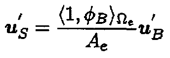
- the degree of freedom of the center of gravity for each element by the operation of static reduction u , U ', u'
- the stability factor control parameter v, (1 ⁇ ⁇ V, ⁇ ) in Eq. (114) is the dimension of the viscosity coefficient (no dimension if the variable corresponding to the viscosity coefficient is made dimensionless). It is a parameter that has a high accuracy solution by appropriately determining this value.
- This method uses the usual Galerkin method for the bubble function element and adds a viscosity term (stabilization action control term) only at the center of gravity to the obtained finite element equation. Tsuyoshi Umetsu, “A Study on Finite Element Analysis of Incompressible Fluids Using Bubble Functions”, Annual Meeting of the Japan Society for Applied Mathematics, 1996, p. 46, p.
- ⁇ in the equation is the viscosity coefficient (diffusion coefficient).
- equation (121) satisfies equation (119).
- equation (124) Set the variable in equation (123) as shown in equation (124) below.
- the stabilization action control term can be introduced and is expressed by the following equation (136).
- the three-level normal ⁇ bubble function can be defined by the following equation (137), and the integral value thereof is expressed by the following equation (138 ) To (142).
- Equation (144) is a matrix consisting of the integral values of the bubble functions of Equations (70), (65), and (66) when the bubble function satisfying Equation (69) is used.
- the stability control parameter V ′ is determined so that the relationship of the following formula (145) is satisfied.
- Equation (146) is a stable matrix that can be expected to improve the analysis accuracy.
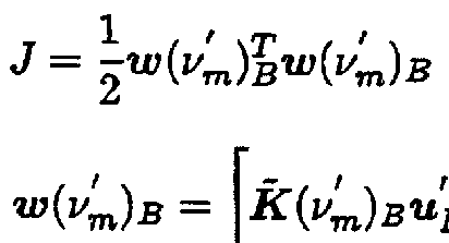
- the problem of determining the stability control parameter V ′ that minimizes the evaluation function of Equation (148) below is determined.
- the stability control parameter V ′ defines the stabilization control parameter V ′ by the number L of unknown analytical physical quantities to be obtained.
- the stabilization action control parameter V ′ m is obtained using the following relational expression (156) which is the stopping condition of 54).
- Equation (155) is a vector, and the vector component is expressed as in the following Equation (157).
- the stabilization control parameter V ′ is m for each vector component.
- Equation (157) shows that the stabilization control parameter V ′ is defined independently for each vector component.
- the stabilizing action control parameter is set so as to satisfy the relationship of the following formula (160).
- V The problem of determining V can also be considered.
- Equation (163) The stability control parameter v ′ is derived from the three-level bubble function of Equation (151).
- the stabilization action control term of Equation (15 2) is derived and the number of unknown analytical physical quantities L Only stable
- the stabilization action control parameter V ′ m is obtained using the following relational expression (166) which is the stopping condition of 64).
- Expression (165) is a vector, and the component of the vector is expressed as the following Expression (167).
- Equation (167) shows that the stability control parameter v 'is defined independently for each vector component.
- V ′ is determined so that the relationship of the following formula (172) is satisfied.
- the stable action is obtained by using the following relational expression (176) that is the stationary condition of the expression (174). Find the control parameters.
- the stability control parameter V ′ defines the stabilization control parameter V ′ by the number L of unknown analytical physical quantities to be obtained using the three-level normal function bubble function of the following equation (177). be able to.
- Equation (171) becomes as shown in Equation (179) below. 5 c
- the first term of equation (179) is a matrix composed of the integral values of the normal ⁇ bubble function of each of the first terms of equations (111) to (113), and equations (70), (65) ( When expressed in 66), it can be described as in the second paragraph.
- V ′ In order to obtain the stable action control parameter V ′ satisfying the relationship of Equation (172), m
- Expression (181) is a vector, and the component of the vector is expressed as the following Expression (183).
- Equation (1 8 3) the stabilization control parameter V ′ is m for each vector component.
- the stabilization action control parameter V ′ m is obtained using the following relational expression (185) which is the stopping condition of 84).
- Equation (183) shows that the stability control parameter v 'is defined independently for each vector component.
- the stabilization control parameter is set so as to satisfy the relationship of the following formula (186).
- V The problem of determining V can also be considered.
- the stabilization action control parameter V ′ m is obtained using the following relational expression (192) that is the stopping condition of 90).
- Expression (191) is a vector, and the vector component is expressed as the following Expression (193).
- Equation (193) shows that the stability control parameter v ′ is defined independently for each vector component m
- the integral value of the bubble function of the equations (70), (65), (6 6), or the integral value of the normalized bubble function of each equation (111) (113) is I need it.
- the extended orthogonal basis bubble function element has the same analysis accuracy as the matched mass matrix because all necessary integral values are given in advance by Equation (80) (without performing complex integration). Very rational in a series of operations that appear in the creation of a diagonal mass matrix and the introduction of the stability control term that improves the numerical instability of the bubble function Can be processed automatically.
- the orthogonal basis bubble function element uses a solution with an efficient storage capacity and calculation time (for example, a four-stage solution), as shown by the analysis results in 2D and 3D. A result can be obtained.
- the expanded orthogonal basal bubble function element conditional expression (80) enables not only inkjet droplet behavior analysis, urban and river inundation analysis, and tsunami generated by earthquakes, but also structural stresses. Because it is possible to handle rationally and consistently the processing required to improve the numerical instability of the bubble function elements and the integral values of the bubble function elements, which are required for analysis, engine natural vibration analysis of automobiles, etc. Therefore, if it can be easily applied to a wide range of numerical analysis as described above, it will produce a drought effect.
- an analysis method with high calculation efficiency such as storage capacity and calculation time (orthogonal basis bubble function element numerical analysis method). ) Can be realized.
- a program prepared in advance is executed by a computer such as a personal computer, workstation, PC cluster, or supercomputer. Can be realized.
- This program is recorded on a computer-readable recording medium such as a hard disk, a flexible disk, a CD-ROM, an MO, and a DVD, and is executed by being read out by the computer.
- the program may be a transmission medium that can be distributed through a network such as the Internet.
- the orthogonal basis bubble function element numerical analysis method, the orthogonal basis bubble function element numerical analysis program, and the orthogonal basis bubble function element numerical analysis apparatus according to the present invention include a mesh of lines, triangles, and tetrahedrons. This is useful for numerical analysis based on the finite element method using.
Landscapes
- Engineering & Computer Science (AREA)
- Physics & Mathematics (AREA)
- Theoretical Computer Science (AREA)
- Computer Hardware Design (AREA)
- Evolutionary Computation (AREA)
- Geometry (AREA)
- General Engineering & Computer Science (AREA)
- General Physics & Mathematics (AREA)
- Management, Administration, Business Operations System, And Electronic Commerce (AREA)
- Complex Calculations (AREA)
Abstract
Description









Claims
Priority Applications (2)
| Application Number | Priority Date | Filing Date | Title |
|---|---|---|---|
| JP2006547876A JP4729767B2 (ja) | 2004-11-26 | 2005-11-25 | 直交基底気泡関数要素数値解析方法、直交基底気泡関数要素数値解析プログラムおよび直交基底気泡関数要素数値解析装置 |
| US11/791,659 US7881912B2 (en) | 2004-11-26 | 2005-11-25 | Orthogonal basis bubble function element numerical analysis method, orthogonal basis bubble function element numerical analysis program, and orthogonal basis bubble function element numerical analyzing apparatus |
Applications Claiming Priority (4)
| Application Number | Priority Date | Filing Date | Title |
|---|---|---|---|
| JP2004-343213 | 2004-11-26 | ||
| JP2004343213 | 2004-11-26 | ||
| JP2005071239 | 2005-03-14 | ||
| JP2005-071239 | 2005-03-14 |
Publications (1)
| Publication Number | Publication Date |
|---|---|
| WO2006057359A1 true WO2006057359A1 (ja) | 2006-06-01 |
Family
ID=36498092
Family Applications (1)
| Application Number | Title | Priority Date | Filing Date |
|---|---|---|---|
| PCT/JP2005/021727 Ceased WO2006057359A1 (ja) | 2004-11-26 | 2005-11-25 | 直交基底気泡関数要素数値解析方法、直交基底気泡関数要素数値解析プログラムおよび直交基底気泡関数要素数値解析装置 |
Country Status (3)
| Country | Link |
|---|---|
| US (1) | US7881912B2 (ja) |
| JP (1) | JP4729767B2 (ja) |
| WO (1) | WO2006057359A1 (ja) |
Families Citing this family (2)
| Publication number | Priority date | Publication date | Assignee | Title |
|---|---|---|---|---|
| CN108595799A (zh) * | 2018-04-12 | 2018-09-28 | 福建省水利水电勘测设计研究院 | 一种大型平开闸排洪防潮运行调度的数值模拟方法 |
| CN110979210B (zh) * | 2019-12-17 | 2021-09-21 | 北京经纬恒润科技股份有限公司 | 整车电源系统配置方法及装置 |
Citations (2)
| Publication number | Priority date | Publication date | Assignee | Title |
|---|---|---|---|---|
| JP2002328955A (ja) * | 2001-04-27 | 2002-11-15 | Keio Gijuku | 質量集中化とデータの再構築および双対格子による数値計算方法 |
| JP2003220808A (ja) * | 2002-01-31 | 2003-08-05 | Yokohama Rubber Co Ltd:The | タイヤ特性予測方法、タイヤ製造方法、空気入りタイヤおよびタイヤ特性予測方法を実行するプログラム |
Family Cites Families (3)
| Publication number | Priority date | Publication date | Assignee | Title |
|---|---|---|---|---|
| WO2004088563A1 (ja) * | 2003-03-31 | 2004-10-14 | National Institute Of Advanced Industrial Science And Technology | 流体解析方法 |
| JP2005115934A (ja) * | 2003-09-16 | 2005-04-28 | National Institute Of Advanced Industrial & Technology | 安定化気泡関数有限要素流体解析方法、安定化気泡関数有限要素流体解析プログラムおよび安定化気泡関数有限要素流体解析装置 |
| JP4604260B2 (ja) * | 2004-09-30 | 2011-01-05 | 学校法人慶應義塾 | GSMAC有限要素法による高次混合要素Poissonソルバーの数値計算手法 |
-
2005
- 2005-11-25 WO PCT/JP2005/021727 patent/WO2006057359A1/ja not_active Ceased
- 2005-11-25 JP JP2006547876A patent/JP4729767B2/ja not_active Expired - Lifetime
- 2005-11-25 US US11/791,659 patent/US7881912B2/en active Active
Patent Citations (2)
| Publication number | Priority date | Publication date | Assignee | Title |
|---|---|---|---|---|
| JP2002328955A (ja) * | 2001-04-27 | 2002-11-15 | Keio Gijuku | 質量集中化とデータの再構築および双対格子による数値計算方法 |
| JP2003220808A (ja) * | 2002-01-31 | 2003-08-05 | Yokohama Rubber Co Ltd:The | タイヤ特性予測方法、タイヤ製造方法、空気入りタイヤおよびタイヤ特性予測方法を実行するプログラム |
Also Published As
| Publication number | Publication date |
|---|---|
| JP4729767B2 (ja) | 2011-07-20 |
| US7881912B2 (en) | 2011-02-01 |
| US20070299641A1 (en) | 2007-12-27 |
| JPWO2006057359A1 (ja) | 2008-06-05 |
| US20080234993A2 (en) | 2008-09-25 |
Similar Documents
| Publication | Publication Date | Title |
|---|---|---|
| Coppola et al. | Discrete energy-conservation properties in the numerical simulation of the Navier–Stokes equations | |
| Maltsev et al. | High-order methods for diffuse-interface models in compressible multi-medium flows: A review | |
| Nguyen et al. | High-order B-splines based finite elements for delamination analysis of laminated composites | |
| Zhu et al. | Computational aspects of stochastic collocation with multifidelity models | |
| Scheufler et al. | TwoPhaseFlow: An OpenFOAM based framework for development of two phase flow solvers | |
| Scheufler et al. | TwoPhaseFlow: A framework for developing two phase flow solvers in OpenFOAM | |
| Hoffman et al. | Unified continuum modeling of fluid-structure interaction | |
| Wu et al. | Simulation of osmotic swelling by the stochastic immersed boundary method | |
| Shivanian et al. | Meshless local radial point interpolation (MLRPI) for generalized telegraph and heat diffusion equation with non-local boundary conditions | |
| Towara | Discrete adjoint optimization with OpenFOAM | |
| Chiappa et al. | Improvement of 2D finite element analysis stress results by radial basis functions and balance equations | |
| Jia | SANM: a symbolic asymptotic numerical solver with applications in mesh deformation | |
| WO2006057359A1 (ja) | 直交基底気泡関数要素数値解析方法、直交基底気泡関数要素数値解析プログラムおよび直交基底気泡関数要素数値解析装置 | |
| Patil et al. | State-of-the-art in different formulations of super convergent mesh-less differential quadrature method | |
| Delchini et al. | Viscous regularization for the non-equilibrium seven-equation two-phase flow model | |
| Stadlmayr et al. | Reduction of physical and constraint degrees-of-freedom of redundant formulated multibody systems | |
| Jafari et al. | An improved three-dimensional model for interface pressure calculations in free-surface flows | |
| JP4032123B2 (ja) | 気泡流シミュレーションプログラム及びそれを記憶した記憶媒体並びに気泡流シミュレーション装置 | |
| Foucard et al. | A particle‐based moving interface method (PMIM) for modeling the large deformation of boundaries in soft matter systems | |
| Hernández et al. | An explicit algorithm for imbedding solid boundaries in Cartesian grids for the reactive Euler equations | |
| Boyanova et al. | Solution methods for the Cahn–Hilliard equation discretized by conforming and non-conforming finite elements | |
| De Souza | How to–Understand Computational Fluid Dynamics Jargon | |
| Burns | Flexible spectral algorithms for simulating astrophysical and geophysical flows | |
| Hiroshi | Variational Multiscale Finite Element Method Based on Bubble Element for Steady Advection-Diffusion Equations | |
| Gosse et al. | Innovative algorithms and analysis |
Legal Events
| Date | Code | Title | Description |
|---|---|---|---|
| AK | Designated states |
Kind code of ref document: A1 Designated state(s): AE AG AL AM AT AU AZ BA BB BG BR BW BY BZ CA CH CN CO CR CU CZ DE DK DM DZ EC EE EG ES FI GB GD GE GH GM HR HU ID IL IN IS JP KE KG KM KN KP KR KZ LC LK LR LS LT LU LV LY MA MD MG MK MN MW MX MZ NA NG NI NO NZ OM PG PH PL PT RO RU SC SD SE SG SK SL SM SY TJ TM TN TR TT TZ UA UG US UZ VC VN YU ZA ZM ZW |
|
| AL | Designated countries for regional patents |
Kind code of ref document: A1 Designated state(s): BW GH GM KE LS MW MZ NA SD SL SZ TZ UG ZM ZW AM AZ BY KG KZ MD RU TJ TM AT BE BG CH CY CZ DE DK EE ES FI FR GB GR HU IE IS IT LT LU LV MC NL PL PT RO SE SI SK TR BF BJ CF CG CI CM GA GN GQ GW ML MR NE SN TD TG |
|
| 121 | Ep: the epo has been informed by wipo that ep was designated in this application | ||
| WWE | Wipo information: entry into national phase |
Ref document number: 2006547876 Country of ref document: JP |
|
| WWE | Wipo information: entry into national phase |
Ref document number: 11791659 Country of ref document: US Ref document number: 200580040495.X Country of ref document: CN |
|
| NENP | Non-entry into the national phase |
Ref country code: DE |
|
| WWP | Wipo information: published in national office |
Ref document number: 11791659 Country of ref document: US |
|
| 122 | Ep: pct application non-entry in european phase |
Ref document number: 05809770 Country of ref document: EP Kind code of ref document: A1 |
|
| WWW | Wipo information: withdrawn in national office |
Ref document number: 5809770 Country of ref document: EP |