US9329263B2 - Imaging system and method - Google Patents
Imaging system and method Download PDFInfo
- Publication number
- US9329263B2 US9329263B2 US13/479,120 US201213479120A US9329263B2 US 9329263 B2 US9329263 B2 US 9329263B2 US 201213479120 A US201213479120 A US 201213479120A US 9329263 B2 US9329263 B2 US 9329263B2
- Authority
- US
- United States
- Prior art keywords
- field
- antenna
- function
- vector
- vie
- Prior art date
- Legal status (The legal status is an assumption and is not a legal conclusion. Google has not performed a legal analysis and makes no representation as to the accuracy of the status listed.)
- Active, expires
Links
Images


Classifications
-
- G—PHYSICS
- G01—MEASURING; TESTING
- G01S—RADIO DIRECTION-FINDING; RADIO NAVIGATION; DETERMINING DISTANCE OR VELOCITY BY USE OF RADIO WAVES; LOCATING OR PRESENCE-DETECTING BY USE OF THE REFLECTION OR RERADIATION OF RADIO WAVES; ANALOGOUS ARRANGEMENTS USING OTHER WAVES
- G01S13/00—Systems using the reflection or reradiation of radio waves, e.g. radar systems; Analogous systems using reflection or reradiation of waves whose nature or wavelength is irrelevant or unspecified
- G01S13/88—Radar or analogous systems specially adapted for specific applications
- G01S13/89—Radar or analogous systems specially adapted for specific applications for mapping or imaging
-
- G—PHYSICS
- G01—MEASURING; TESTING
- G01S—RADIO DIRECTION-FINDING; RADIO NAVIGATION; DETERMINING DISTANCE OR VELOCITY BY USE OF RADIO WAVES; LOCATING OR PRESENCE-DETECTING BY USE OF THE REFLECTION OR RERADIATION OF RADIO WAVES; ANALOGOUS ARRANGEMENTS USING OTHER WAVES
- G01S13/00—Systems using the reflection or reradiation of radio waves, e.g. radar systems; Analogous systems using reflection or reradiation of waves whose nature or wavelength is irrelevant or unspecified
- G01S13/88—Radar or analogous systems specially adapted for specific applications
-
- G—PHYSICS
- G01—MEASURING; TESTING
- G01S—RADIO DIRECTION-FINDING; RADIO NAVIGATION; DETERMINING DISTANCE OR VELOCITY BY USE OF RADIO WAVES; LOCATING OR PRESENCE-DETECTING BY USE OF THE REFLECTION OR RERADIATION OF RADIO WAVES; ANALOGOUS ARRANGEMENTS USING OTHER WAVES
- G01S7/00—Details of systems according to groups G01S13/00, G01S15/00, G01S17/00
- G01S7/02—Details of systems according to groups G01S13/00, G01S15/00, G01S17/00 of systems according to group G01S13/00
- G01S7/41—Details of systems according to groups G01S13/00, G01S15/00, G01S17/00 of systems according to group G01S13/00 using analysis of echo signal for target characterisation; Target signature; Target cross-section
- G01S7/411—Identification of targets based on measurements of radar reflectivity
- G01S7/412—Identification of targets based on measurements of radar reflectivity based on a comparison between measured values and known or stored values
-
- G01S2007/4082—
-
- G—PHYSICS
- G01—MEASURING; TESTING
- G01S—RADIO DIRECTION-FINDING; RADIO NAVIGATION; DETERMINING DISTANCE OR VELOCITY BY USE OF RADIO WAVES; LOCATING OR PRESENCE-DETECTING BY USE OF THE REFLECTION OR RERADIATION OF RADIO WAVES; ANALOGOUS ARRANGEMENTS USING OTHER WAVES
- G01S7/00—Details of systems according to groups G01S13/00, G01S15/00, G01S17/00
- G01S7/02—Details of systems according to groups G01S13/00, G01S15/00, G01S17/00 of systems according to group G01S13/00
- G01S7/40—Means for monitoring or calibrating
- G01S7/4052—Means for monitoring or calibrating by simulation of echoes
- G01S7/4082—Means for monitoring or calibrating by simulation of echoes using externally generated reference signals, e.g. via remote reflector or transponder
Definitions
- the present invention generally relates to imaging systems and methods and, more particularly, to systems and methods that image or otherwise provide information regarding the electromagnetic and/or mechanical properties of the objects being evaluated.
- an imaging method that includes the steps of: (a) determining an incident field, (b) using the incident field and a volume integral equation (VIE) to determine a total field, (c) predicting voltage ratio measurement at a receiving antenna by using the volume integral equation (VIE), wherein the VIE includes a vector Green's function, (d) collecting voltage ratio measurements from one or more receiving antennas, and (e) comparing the predicted voltage ratio measurements to the collected voltage ratio measurements to determine one or more properties of the object being evaluated.
- VIE volume integral equation
- an imaging system that includes at least one transmitting antenna for transmitting probing field radiation towards a target object, at least one receiving antenna for receiving at least some of the radiation that is scattered by the target object, and a computer-based data collection system that operates to determine an incident field related to the transmitted radiation, determine a total field, compute a receiving antenna voltage ratio measurement using a volume integral equation (VIE) that includes a vector Green's function, receives actual voltage ratio measurements from the one or more receiving antennas, and determines at least one property of the target object using the computed voltage ratio measurement and the actual voltage ratio measurements.
- VIE volume integral equation
- FIG. 1 is a flowchart depicting an embodiment of an imaging method in accordance with the invention
- FIG. 2 is a block diagram of a data collection system that may be used with transmitting and receiving antennas to carry out the method of FIG. 1 ;
- FIGS. 3-5 depict different antenna setups for use with the method of FIG. 1 and the data collection system of FIG. 2 ;
- FIGS. 6 and 7 are diagrammatic views of antenna and transmission line setups
- FIG. 8 shows a network model of two antennas and a scattering object
- FIG. 9 shows an antenna and transmission line setup for an object-centered scattering scenario
- FIG. 10 shows an example setup using a transmitting and receiving waveguides and a target object comprising a pair of acrylic spheres
- FIG. 11 depicts the discretized object domain for the example setup of FIG. 10 ;
- FIG. 12 shows magnitude and phase plots of the measured and predicted S 21 S-parameters for the example setup of FIG. 10 ;
- FIG. 13 shows a second example setup for a single acrylic sphere placed in an anechoic chamber
- FIG. 14 shows one of the waveguides and the single and pair of acrylic spheres used in the first and second examples
- FIG. 15 shows magnitude and phase plots of the measured and predicted S 11 S-parameters for the example setup of FIG. 13 ;
- FIG. 16 is an HFSS CAD model for a third example which uses a simulation of two different sized apertures embedded within PEC walls;
- FIG. 17 shows magnitude and phase plots of simulated and predicted S 21 and S 12 S-parameters for the simulated third example
- FIG. 18 shows magnitude and phase plots of simulated and predicted S 11 and S 22 S-parameters for the simulated third example
- FIG. 19 shows components for a dielectrically loaded waveguide for a fourth example with the empty waveguide shown along with two nylon blocks that make up the load and object domains;
- FIG. 20 is an HFSS CAD model of the assembled dielectrically loaded waveguide of FIG. 19 ;
- FIG. 21 shows magnitude and phase plots of the measured, simulated, and predicted S 21 S-parameters for the example setup of FIGS. 19 and 20 ;
- FIG. 22 shows magnitude and phase plots of the measured, simulated, and predicted S 11 and S 22 S-parameters for the example setup of FIGS. 19 and 20 ;
- FIG. 23 is a block diagram of an inverse scattering process
- FIG. 24 shows a network model of two antennas and a scattering object, as in FIG. 8 ;
- FIG. 25 shows an antenna setup used to test the inverse scattering method of FIG. 23 using fifteen antennas arranged around a target object;
- FIG. 26( a ) is an HFSS CAD model of an E-patch antenna in vertical polarization
- FIG. 26( b ) shows an actual antenna mounted in the test setup of FIG. 25 for horizontal polarization
- FIG. 27 shows magnitude and phase plots of the simulated and measured S 11 S-parameters for the E-patch antennas used in the setup of FIG. 25 ;
- FIG. 28 is a plot of normalized magnitudes of transit coefficients for the E-patch antennas used in the setup of FIG. 25 ;
- FIG. 29 is a schematic of ideal antenna reference frame positions and rotations for the antenna setup of FIG. 25 ;
- FIG. 30 shows a test setup for testing the antenna model using a conducting sphere centered in the antenna array
- FIG. 31 shows magnitude and phase plots of measured and predicted S 21 of the incident, total and scattered fields of the conducting sphere of FIG. 30 ;
- FIG. 32 is a histogram of the real part of S 21 of the incident field of the receiving antenna located across from the transmitting antenna;
- FIG. 33( a ) is a photo of the target objects and FIGS. 33( b )-33( d ) show reconstructed relative permittivities at different conjugate gradient iterations carried out during the inverse scattering method of FIG. 23 ;
- FIG. 34( a ) shows a normalized residual for conjugate gradient iterations for each successive BMI iteration carried out as a part of the inverse scattering method of FIG. 23 ;
- FIG. 34( b ) shows a vertical cut of the actual and reconstructed relative permittivity through the center of the two target objects shown in FIG. 33( a ) ;
- FIG. 35( a ) shows a reconstructed image of the two target objects using HH polarization data.
- FIG. 35( b ) a vertical cut of the actual and reconstructed relative permittivity through the center of the two target objects shown in FIG. 33( a ) ;
- FIG. 36( a ) is a photo of the target objects
- FIG. 36( b ) shows a reconstructed image of the relative permittivity
- FIG. 36( c ) shows normalized residual for all BIM iterations
- FIG. 36( d ) shows a horizontal cut through the middle of the image for the actual and reconstructed object
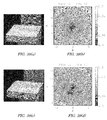
- FIGS. 37( a ) and 37( c ) show PCV rings (tubes) used as target objects and FIGS. 37( b ) and 37( d ) show respective reconstructed relative permittivities after twelve BIM iterations;
- FIGS. 38( a ) and 38( c ) show target object setups using an outer ring (tube) and eccentric inner cylinder, and FIGS. 38( b ) and 38( d ) show respective reconstructed relative permittivities after twelve BIM iterations;
- FIGS. 39( a ) and 39( c ) show target object setups using two metal rods at different spacings, and FIGS. 39( b ) and 39( d ) show respective reconstructed relative permittivities after twelve BIM iterations;
- FIG. 40( a ) shows another test setup using a ring and eccentric cylinder and FIG. 40( b ) shows a reconstructed relative permittivity after 12 BIM iterations;
- FIG. 41( a ) shows a rod and block test steup and FIG. 41( b ) shows a reconstructed relative permittivity after 12 BIM iterations;
- FIG. 42( a ) shows objects used to generate synthetic scattered field data and FIG. 42( b ) shows a reconstruction of the objects using synthetic data;
- FIG. 43( a ) shows an image reconstruction of a cylinder and block test object using synthetic data and FIG. 43( b ) shows a reconstruction of the objects using experimental data.
- Imaging method 10 may be used to non-invasively produce an image of one or more properties of an object, such as the object's permittivity, susceptibility, conductivity, density, compressibility, acoustic loss, etc.
- Imaging method 10 may be used in a wide variety of non-invasive imaging applications, such as those in the medical field where soft tissue is evaluated, those in the logistical field where packages and other objects need to be inspected without being opened, and those in the scientific field where samples are analyzed for their constituent parts, just to name a few possibilities.
- method 10 helps screen and evaluate human or animal tissue for cancer (e.g., breast cancer, brain tumors, etc.) and may be used to supplement current screening techniques, as it provides the physician with yet another tool for discerning between benign and malignant tissue.
- cancer e.g., breast cancer, brain tumors, etc.
- imaging method 10 helps screen and evaluate human or animal tissue for cancer (e.g., breast cancer, brain tumors, etc.) and may be used to supplement current screening techniques, as it provides the physician with yet another tool for discerning between benign and malignant tissue.
- imaging method 10 is described below in the context of electromagnetic waves, it should be appreciated that the method may be used with mechanical waves as well.
- the imaging method may generate an image of one or more of the electromagnetic properties of the object being evaluated (e.g., the object's permittivity, susceptibility, conductivity and/or other dielectric properties); in the mechanical wave embodiment, the imaging method may generate an image of one or more of the mechanical properties of the object (e.g., the object's density, compressibility, acoustic loss, etc.).
- FIG. 1 is only meant to be a high-level illustration of the overall structure of an exemplary imaging method 10 and that each of the method steps may include any number of different sub-steps and techniques.
- imaging method 10 generally includes the steps of: exciting one or more transmitting antennas with a voltage excitation (ref), step 11 ; determining the incident field in the object domain due to the voltage excitation on the transmitting antennas, step 12 ; using the incident field and a volume integral equation (VIE) to determine a total field for the object being evaluated, step 13 ; predicting the scattered field voltage excitations at a receiving antenna by using the volume integral equation (VIE), which includes using a vector Green's function for a receiving antenna, step 14 ; collecting scalar voltage ratio measurements from one or more receiving antennas, step 15 ; and, using the scalar voltage ratio measurements and an inverse scattering algorithm to determine one or more properties of the object being evaluated 20 , step 16 .
- VIE volume integral equation
- step 12 may determine the incident field in the object domain by one or more of the following techniques: i) using an antenna model to determine one or more expansion coefficients, and then using the expansion coefficients and a multipole expansion to determine the incident field; ii) measuring the incident field through experiment; and/or iii) estimating the incident field using simulation.
- VIE volume integral equation
- An inhomogeneous object is represented by a material contrast relative to the background, and the kernel of the VIE is the background dyadic Green's function.
- the dyadic Green's function can be used either to determine the total field solution inside the object domain or to move the field quantities inside the object domain to observed fields outside the object domain.
- this type of formulation may be indispensable for analytic and numerical studies, the vector fields predicted by the VIE in the latter case may not be observed directly in measurement. That is, actual measurements of fields are performed with antennas or probes, the outputs of which are voltage excitations, which are scalar quantities.
- method 10 uses a kernel which, instead of relating fields to fields, relates fields to scalars.
- method 10 may not only link the VIE directly to measurement quantities, it also may be used to link it to S-parameter measurements.
- the antenna model used in method 10 is based on the source-scattering matrix formulation. This model relates the multipole fields radiated and received by an antenna to the incoming and outgoing voltages on a feeding transmission line.
- the antenna model can manifest itself as a new kernel which moves field quantities in the object domain to a scalar voltage on the transmission line. Because of the role this new kernel serves in the VIE, it is broadly referred to here as a “vector Green's function,” and can be used to predict an object's scattered field S-parameters measured in a mono-static or bi-static antenna system.
- the vector Green's function may be used only in a measurement role. Such a case may be analogous to when the observation point argument of the dyadic Green's function is evaluated at a receiver location.
- the vector Green's function implicitly includes the antenna model.
- the vector Green's function is not used to simulate the forward scattering of an object, nor is it to be confused with functions where it is one column of the dyadic Green's function or where it is defined by the gradient of the scalar green's function.
- method 10 calibrates the antenna output by converting voltages excitations to radiated fields and does so based on a variation of the electric field volume integral equation (VIE) for inhomogeneous media that is tailored for microwave S-parameter measurements.
- VIE electric field volume integral equation
- the kernel of the standard VIE is a dyadic Green's function which can relate fields in the object domain to observed scattered fields outside the object domain
- the kernel in method 10 is a vector Green's function which can relate fields in the object domain to S-parameter measurements outside the object domain.
- the exemplary kernel or formulation may directly link properties of the object being evaluated (e.g., permittivity, susceptibility, conductivity and/or other dielectric properties) to measurements being received, and it may do so in a way that is useful to many applications (e.g., microwave applications).
- properties of the object being evaluated e.g., permittivity, susceptibility, conductivity and/or other dielectric properties
- the dyadic Green's function is related to the incident field produced by an infinitesimal source.
- the vector Green's function may be related to the incident field produced by an antenna and proper scaling factors may be found.
- the primary derivation is for antennas and objects in free-space, it should be appreciated that the relationship between the vector Green's function and the antenna incident field holds whether or not there exist closed form expressions for either. This implies that simulation may be used to estimate the vector Green's function for any complex measurement geometry where it will include all background multiple scattering not included in the VIE object function.
- step 11 excites one or more transmitting antennas (e.g., an antenna array) with voltage excitations (ref), and may do so in any number of different ways.
- FIGS. 2-5 show several different exemplary systems and setups that may be used with step 11 , including data collection system 20 .
- data collection system 20 includes user input 22 , computer 24 , radar control 26 , radar system 28 , data interface 30 , switch 32 , and antenna array 34 .
- antenna array 34 includes one transmitting antenna 40 and a number of receiving antennas 42 circumferentially surrounding a target or object being evaluated 44 (e.g., human tissue) so that electromagnetic waves can be reflected off of the target and evaluated.
- Transmitting antenna 40 and receiving antennas 42 are connected to switch 32 , which may act like a multiplexor of sorts by individually receiving and transmitting the output from the various antennas.
- switch 32 goes around the antenna array, sequentially accepting output from the different receiving antennas, and packages and sends the antenna output to radar system 28 .
- Antenna array 34 may include one or more square patch antennas or any other suitable antenna type, and radar system 28 may include a two-port Vector Network Analyzer (VNA), as is understood by those skilled in the art.
- VNA Vector Network Analyzer
- transmitting antenna 40 emits radar waves that impinge target 44 and reflect or scatter off of the target accordingly.
- Receiving antennas 42 which circumferentially surround target 44 , gather the reflected radar waves and provide them back to radar system 28 so that an image can be formed of one or more electromagnetic properties of the target or object 44 that is being evaluated.
- Data interface 30 may be used to process or couple the raw data or information from radar system 28 to computer 24 (e.g., to convert the data from an analog format to a digital one).
- data collection system 20 functions as a multistatic radar system using the antenna array 34 .
- the radar waves are transmitted through free space. That is, target 44 is simply placed on a pedestal or other support and is surrounding by the free space atmosphere at that location.
- the embodiment shown in FIG. 4 includes a chamber 50 that surrounds or encompasses target 44 so that the space within the chamber can be filled with a liquid medium 52 having a high dielectric constant and moderate loss (e.g., an oil-water emulsion).
- the liquid medium 52 should be coupled or matched to target 44 , and may be selected to work with electromagnetic waves of a certain wavelength, etc.
- step 11 is not limited to the exemplary system shown in FIG. 1 nor is it limited to radio waves or even electromagnetic waves, as mentioned above.
- Data collection system 20 could use a mono-static, bi-static or other multi-static antenna system in place of the exemplary system shown in the FIGS. 3-5 , to cite a few possibilities.
- the method determines the incident field E inc (r) in the object domain, step 12 .
- Step 12 determines the incident field E inc (r) in the object domain due to the voltage excitation on the transmitting antennas, and may do so in a number of different ways. This step, in combination with some of the other steps of method 10 , is sometimes referred to as “calibrating,” and is described below with a number of derivations.
- VIE electric field volume integral equation
- E ⁇ ( r ) E inc ⁇ ( r ) + k o 2 ⁇ ⁇ G _ ⁇ ( r , r ′ ) ⁇ ( ⁇ ⁇ ( r ′ ) + i ⁇ ⁇ ⁇ ⁇ ( r ′ ) ⁇ b ⁇ w ) ⁇ E ⁇ ( r ′ ) ⁇ d V ′ ( 1 )
- E(r) and E inc (r) are the total and incident fields, respectively
- r is the observation position vector
- ⁇ b ⁇ o ⁇ rb is the background permittivity with relative permittivity ⁇ rb .
- ⁇ b is the background conductivity
- ⁇ (r) is unitless
- ⁇ (r) is an absolute measure of conductivity with units of Siemens per meter
- G (r,r′) is the dyadic Green's function for the background medium. In free space, this is given by
- G _ ⁇ ( r , r ′ ) [ I _ + ⁇ ′ ⁇ ⁇ ′ k 2 ] ⁇ g ⁇ ( r , r ′ ) ⁇ ⁇
- the background wave number, k is given by
- k 2 k o 2 ⁇ ( 1 + i ⁇ ⁇ b ⁇ b ⁇ ⁇ ) ( 6 )
- E ⁇ ( r ) ⁇ lm ⁇ ⁇ [ a lm ⁇ M lm ⁇ ( r ) + b lm ⁇ N lm ⁇ ( r ) + c lm ⁇ ⁇ M lm ⁇ ( r ) + d lm ⁇ ⁇ N lm ⁇ ( r ) ] ( 10 )
- r is the position vector
- the quantities M lm (r) and N lm (r) are the free-space vector wave functions, and means the regular part of the corresponding spherical Bessel function.
- the conventions for vector wave functions are given by,
- M lm ⁇ ( r ) ⁇ ⁇ [ rz l ⁇ ( kr ) ⁇ Y lm ⁇ ( ⁇ , ⁇ ) ] ( 11 )
- N lm ⁇ ( r ) 1 k ⁇ ⁇ ⁇ M lm ⁇ ( r ) ( 12 )
- z l (kr) is any spherical Bessel function
- Y lm ( ⁇ , ⁇ ) are the angular harmonics.
- a lm and b lm are the expansion coefficients for outgoing waves
- c lm and d lm are the coefficients for incoming waves.
- the number of harmonics needed to represent a field produced by an antenna is O(kd), where d is the largest dimension of the antenna.
- the full antenna response is modeled following the source-scattering matrix formulation.
- the antenna is connected to a shielded transmission line, as shown in FIG. 6 , where a o and b o are complex outgoing and incoming voltages, respectively, on the transmission line.
- the voltages on the transmission line are related to the multipole expansion coefficients through a linear antenna model that is written as,
- b o ⁇ ⁇ lm ⁇ ⁇ ( u ( c ) ⁇ lm ⁇ c lm + u ( d ) ⁇ lm ⁇ d lm ) ( 13 )
- a lm a o ⁇ t ( a ) ⁇ lm ( 14 )
- b lm a o ⁇ t ( b ) ⁇ lm ( 15 )
- u (c)lm and u (d)lm are receive coefficients which convert incoming field harmonics to b o .
- t (a)lm and t (b)lm are transmit coefficients which convert a o to outgoing field harmonics.
- k is the wavenumber of the medium
- ⁇ is the operating frequency in radians
- ⁇ is the background permeability
- Z o is the characteristic impedance of the transmission line.
- the incident field produced by a transmitting antenna is composed of only outgoing waves.
- E inc has units of V/m and a o has units of V, so e inc has units of 1/m.
- step 12 may alternatively measure the incident field through experimentation and/or estimate the incident field using simulation. Other methods and techniques for determining the incident field may be used as well. Once the incident field has been determined, the method determines the total field for the object being evaluated, step 13 .
- Step 13 uses the incident field and a volume integral equation (VIE) to determine a total field for the object being evaluated, and may do so in a number of different ways.
- VIE volume integral equation
- e(r) as the normalized total field. This is the field solution resulting from a normalized incident field. That is, the field solution due to a source described by only the transmit coefficients. Similar to e inc (r), e(r) also has units of 1/m.
- the method predicts the scattered field voltages at a receiving antenna, step 14 .
- Step 14 predicts the scattered field voltages at a receiving antenna by using the volume integral equation (VIE), which includes using a vector Green's function.
- VIE volume integral equation
- the dyadic Green's function which is the kernel of a traditional VIE, serves to move field quantities inside the object region to field quantities outside the object region.
- Step 14 uses an additional modeling step to convert the fields at observation points to voltages, and the antenna model described previously is one mechanism to do this.
- the antenna model may manifest itself concisely as a new kernel, which, instead of transforming fields to fields, transforms fields to scalars.
- the new kernel of step 14 can move field quantities inside the object region directly to scalar measurement quantities outside the object region.
- This kernel is a vector as opposed to a dyad; thus, it is referred to here as the vector Green's function. Because the antenna model links the fields of an antenna to the voltages on its feeding transmission line, using the concept of normalized fields, the vector Green's function is specialized for S-parameter measurements.
- the scattered field from the VIE is expanded as incoming waves in the reference frame of the receiver.
- G _ ⁇ ( r , r ′ ) ik ⁇ ⁇ lm ⁇ ⁇ 1 l ⁇ ( l + 1 ) ⁇ [ ⁇ M lm ⁇ ( r ) ⁇ M ⁇ lm ⁇ ( r ′ ) + ⁇ N lm ⁇ ( r ) ⁇ N ⁇ lm ⁇ ( r ′ ) ] ( 24 )
- hat, ⁇ denotes conjugating the angular part of the vector wave function.
- the dyad is formed by taking the outer product of M lm (r) and ⁇ circumflex over (M) ⁇ lm (r′), and of N lm (r) and ⁇ circumflex over (N) ⁇ lm (r′).
- r and r′ are position vectors in the frame of the receiver where
- E sca ⁇ ( r ) ⁇ ( ik ⁇ ⁇ lm ⁇ ⁇ 1 l ⁇ ( l + 1 ) ⁇ [ ⁇ M lm ⁇ ( r ) ⁇ M ⁇ lm ⁇ ( r ′ ) + ] ) ⁇ O ⁇ ( r ′ ) ⁇ E ⁇ ( r ′ ) ⁇ ⁇ d V ′ ( 25 )
- the scattered field of the VIE can be written as incoming fields in the frame of the receiver as,
- E sca ⁇ ( r ) ⁇ lm ⁇ ⁇ ( c lm ⁇ ⁇ M lm ⁇ ( r ) + d lm ⁇ ⁇ N lm ⁇ ( r ) ) ( 26 ) where the expansion coefficients are
- c lm ik l ⁇ ( l + 1 ) ⁇ ⁇ M ⁇ lm ⁇ ( r ′ ) ⁇ O ⁇ ( r ′ ) ⁇ E ⁇ ( r ′ ) ⁇ d V ′ ( 27 )
- d lm ik l ⁇ ( l + 1 ) ⁇ ⁇ N ⁇ lm ⁇ ( r ′ ) ⁇ O ⁇ ( r ′ ) ⁇ E ⁇ ( r ′ ) ⁇ d V ′ ( 28 )
- the quantity O(r)E(r) can be thought of as a collection of infinitesimal dipole current sources.
- the vector wave functions in the integrands of Eqns. (27) and (28) effectively translate the fields radiated from these dipoles so as to be expanded as incoming waves in the frame of the receiver. This action can be compared to the translation of dipole fields in the context of T-matrix methods.
- translating dipole fields using the translation matrices for vector spherical harmonics only requires the first three columns of the matrices.
- the matrix entries have Hankel functions for the radial part, and the vector argument points from the dipole to the receiver.
- the incoming field coefficients are the aggregates of all translated dipole fields.
- g ⁇ ( r ′ ) ik ⁇ ⁇ lm ⁇ ⁇ 1 l ⁇ ( l + 1 ) ⁇ ( u ( c ) ⁇ lm ⁇ M ⁇ lm ⁇ ( r ′ ) + u ( d ) ⁇ lm ⁇ N ⁇ lm ⁇ ( r ′ ) ) ( 32 )
- the vector Green's function for the free-space VIE is a sum of dipole translations weighted by the receive coefficients of the antenna. It directly links field quantities in the object domain to the incoming voltage on the receiver transmission line.
- the traditional scattered field volume integral equation has been transformed into one suitable for S-parameter measurements.
- the notation, S ji can be read similarly to its use for multi-port networks, where this is the scattered field S-parameter measured by a receiver in frame j due to a transmitter in frame i.
- Eqn. (34) has been derived in a bi-static S 21 measurement setup, it also applies to monostatic S 11 measurements.
- the S-parameters are measured between the reference planes on the antenna transmission lines, so that the antennas and the object scattering are represented by a 2-port microwave network, shown in FIG. 8 , which is a network model of two antennas and a scattering object where S-parameters are measured between the reference planes on the antenna transmission lines.
- the vector Green's function is only used in a measurement role; it is not used to simulate the forward scattering of an object.
- Eqn. (1) or Eqn. (21) in its entirety using one of numerous techniques, e.g. Conjugate Gradient FFT, Neumann Series, Finite Difference Time Domain, etc.
- the forward solvers also require knowledge of the incident field throughout the object domain.
- the normalized incident field is computed using Eqn. (20).
- g ⁇ ( r ) ⁇ iZ 0 2 ⁇ ⁇ ⁇ ⁇ ⁇ ⁇ ⁇ lm ⁇ ⁇ ( t ( a ) ⁇ lm ⁇ M lm ⁇ ( r ) + t ( b ) ⁇ lm ⁇ N lm ⁇ ( r ) ) ( 40 ) which is the expansion for the normalized incident field multiplied by a scaling factor
- the vector Green's function used in the VIE for a receiver can be interpreted as the incident field produced by that antenna in transmit mode and scaled by factors characterizing the transmission line.
- This form of the vector Green's function means the step of determining the antenna transmit and receive coefficients can be bypassed, if we can obtain and store the incident field with other means, such as simulation.
- the following description pertains to object-centered vector Green's function.
- the vector Green's function was derived for a receiver-centered scattering situation.
- the object can surround the receiver.
- multiple antennas usually surround the object.
- the antenna model and derivation can be reworked for an object-centered situation, where we will be dealing with the condition
- FIG. 9 shows an antenna and transmission line setup for an object-centered scattering scenario.
- the quantities a 0 and b 0 are outgoing and incoming voltages on the transmission line, respectively.
- the dotted line represents the furthest point of non-zero contrast.
- the multipole expansion of the electric field is the same as before, Eqn. (10), but now it is expanded in the frame of the object instead of the antenna.
- the antenna model is,
- u (a)lm and u (b)lm are the receive coefficients which convert outgoing field harmonics in the frame of the object to b o .
- c lm and d lm are transmit coefficients which convert a o to incoming field harmonics in the frame of the object.
- G _ ⁇ ( r , r ′ ) i ⁇ ⁇ k ⁇ ⁇ l ⁇ ⁇ m ⁇ 1 l ⁇ ( l + 1 ) ⁇ [ M l ⁇ ⁇ m ⁇ ( r ) ⁇ ⁇ ⁇ M ⁇ l ⁇ ⁇ m ⁇ ( r ′ ) + N l ⁇ ⁇ m ⁇ ⁇ N ⁇ l ⁇ ⁇ m ⁇ ( r ′ ) ] ( 49 ) Substituting this into the VIE provides the scattered field in terms of outgoing coefficients in the frame of the object
- E sca ⁇ ( r ) ⁇ l ⁇ ⁇ m ⁇ [ a l ⁇ ⁇ m ⁇ M l ⁇ ⁇ m ⁇ ( r ) + b l ⁇ ⁇ m ⁇ N l ⁇ ⁇ m ⁇ ( r ) ] ⁇ ⁇
- a l ⁇ ⁇ m i ⁇ ⁇ k l ⁇ ( l + 1 ) ⁇ ⁇ ⁇ M ⁇ l ⁇ ⁇ m ⁇ ( r ′ ) ⁇ O ⁇ ( r ′ ) ⁇ E ⁇ ( r ′ ) ⁇ d V ′
- b l ⁇ ⁇ m i ⁇ ⁇ k l ⁇ ( l + 1 ) ⁇ ⁇ ⁇ N ⁇ l ⁇ ⁇ m ⁇ ( r ′ ) ⁇ O ⁇ ( r ′ ) ⁇ E
- the integration vector r′ now points from the origin of the object frame to an integration point still in the object domain.
- the vector wave functions in the integrands are translating the dipole fields to the origin of the object frame.
- a lm and b lm are the coefficients for the multipole expansion of the scattered field radiating from the object. This also means that the antennas cannot be inside a sphere with a radius smaller than the furthest point of non-zero contrast from the origin of the object frame, as shown in FIG. 9 .
- g ⁇ ( r ′ ) i ⁇ ⁇ k ⁇ ⁇ ⁇ ⁇ l ⁇ ⁇ m ⁇ 1 l ⁇ ( l + 1 ) ⁇ ( u ( a ) ⁇ l ⁇ ⁇ m ⁇ ⁇ M ⁇ l ⁇ ⁇ m ⁇ ( r ′ ) + u ( b ) ⁇ l ⁇ ⁇ m ⁇ N ⁇ l ⁇ ⁇ m ⁇ ( r ′ ) ) ( 54 )
- E inc ⁇ ( r , r p ) i ⁇ ⁇ ⁇ ⁇ ⁇ ⁇ I ⁇ G _ ⁇ ( r , r p ) ⁇ p ⁇ ⁇ ⁇ or ( 57 )
- G _ ⁇ ( r , r p ) ⁇ p ⁇ 1 i ⁇ ⁇ ⁇ ⁇ ⁇ I ⁇ E inc ⁇ ( r , r p ) ( 58 )
- the columns of the dyadic green's function can be found by finding the incident field due to three orthogonal dipoles in turn.
- the arguments r and r p can be swapped, which will provide the dyadic Green's function used in the VIE to predict observed scattered fields at the point r p by integrating over the points r.
- this technique can be used for any problem geometry, not only free-space, and has been used in simulation for nonlinear inverse scattering algorithms.
- the following description pertains to obtaining g(r). Determining the antenna transmit and receive coefficients can be difficult. These are the same transmit and receive coefficients that can be obtained from near-field antenna measurements. Near-field systems are expensive ventures, which require precise positioning and probe calibration. Alternatively, these coefficients can be estimated using simulation, from which g (r) can be computed using Eqn. (32) or Eqn. (40). However, from Eqn. (41), it is sufficient to simply know the incident field, which can be determined through measurement or estimated with simulation.
- the phase of a o is found by comparing the transmission line reference plane used to determine the simulated fields to those used in measurement by, for instance, a vector network analyzer (VNA).
- VNA vector network analyzer
- G _ ⁇ ( r , r ′ ) ⁇ ⁇ ⁇ [ k ′ ⁇ M ⁇ ⁇ ( r ) ⁇ M ⁇ * ⁇ ( r ′ ) + k ′′ ⁇ N ⁇ ⁇ ( r ) ⁇ N ⁇ * ⁇ ( r ′ ) ] ( 61 )
- M ⁇ (r) and N ⁇ (r) are the electric and magnetic (or vice versa) solenoid vector wave functions, with adjoints (or inverses) M*(r) and N*(r) and k′ and k′′ are their normalizations.
- Step 15 collects scalar voltage ratio measurements from one or more receiving antennas, and step 16 uses the scalar voltage ratio measurements and an inverse scattering algorithm, which may include a number of the previous steps, to determine one or more properties of the object being evaluated. Steps 15 and 16 may be performed in a number of different ways.
- measured and predicted scattered field S 21 is determined in free space for a pair of dielectric spheres.
- the waveguides and spheres are shown in FIG. 10 .
- the waveguides are hollow brass having WR-187 specification operating between 4-6 GHz with outer dimensions of 2.54 cm ⁇ 5.08 cm ⁇ 15.2 cm, and fed with SMA extended dielectric flange mount connectors.
- the waveguides are characterized using Ansoft HFSS and a multipole and S-parameter method that uses HFSS to simulate the fields radiated by the antenna, which are used to estimate the antenna transmit coefficients.
- the transmit coefficients can then be used in Eqn. (20) to compute the normalized incident field at any points around the antenna except those in the very near-field.
- the setup for this example is shown in FIG. 10 , where two waveguides are rotated 120 degrees around the target at distances of 16 inches apart.
- the waveguides are placed on a Styrofoam board which is suspended on a Styrofoam pedestal in an anechoic chamber. Measurements were taken between 4-6 GHz.
- the transmitter and receiver are positioned 40.6 cm away from the scatterers.
- the transmitter is fixed and the receiver is positioned in 15 degree increments about the center from 90 to 180 degrees relative to the transmitter.
- the spheres are acrylic and identical, having a diameter of 2.54 cm and a relative permittivity of 2.5 and assumed lossless.
- the spheres are held in a Styrofoam support and separated by approximately 5 cm.
- S 21 is predicted using Eqn. (43) at 21 discrete frequencies between 4-6 GHz.
- an object domain is defined encompassing the two spheres with dimensions 9 cm ⁇ 9 cm ⁇ 5 cm.
- the object domain is discretized with a regular spacing of 2.5 mm, which is ⁇ /20 at 6 GHz in a material with relative permittivity of 2.5.
- the discretized domain and the dielectric contrast of the pair of spheres are shown in FIG. 11 , which illustrates the discretized object domain for this example.
- the transmit coefficients and Eqn. (20) the normalized incident field of the transmitter is computed at all points in the object domain. This is used to compute the normalized total field in the object region using the Bi-Conjugate Gradient FFT (BCGFFT).
- BCGFFT Bi-Conjugate Gradient FFT
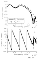
- FIG. 12 shows the magnitude and phase of measured and predicted S 21 for the scattered field for the pair of spheres at receiver angles of 120 degrees and 180 degrees (see also FIG. 10 ).
- Solid line and dots illustrate measured and predicted S 21 for a receiver at 180 degrees
- dashed line and triangles illustrate S 21 for a receiver at 120 degrees, where the second set of phases is shifted by 360 degrees for display.
- the magnitude of measured and predicted S 21 agree to better than 2 dB across the band (at ⁇ 50 dB levels or less).
- the phase agrees overall to better than 20 degrees.
- VIE can be used in conjunction with the vector Green's function and a numeric volumetric forward solver to predict S 21 for the scattered field with a phase much better than ⁇ /10, i.e., 36 degrees, which is a common metric for many microwave systems.
- Eqn. (43) is used to predict S 11 for the setup in FIG. 13 .
- the same procedure is used as in the first exemplary experiment, however, here the scattered field S 11 are predicted for a single acrylic sphere.
- One waveguide is supported by Styrofoam in an anechoic chamber, show in FIG. 13 .
- the sphere is held in a Styrofoam and placed two inches in front of the waveguide and one inch to the side of the boresight.
- the Stryofoam holder is included in the incident field measurement, and it is shown in FIG. 14 .
- the normalized total field in the object region is computed again with the BCGFFT.
- the same incident field is used for the vector Green's function because we are predicting S 11 .
- a test is performed for the vector Green's function and VIE in simulation. Simulated and predicted scattered field S-parameters are compared of an arbitrary distribution of inhomogeneous dielectric objects in a near-field scenario using HFSS. No assumptions are made about the nature of the field solution. This example supports the argument that Eqn. (41) holds for any geometry.
- the simulation domain is shown in FIG. 16 , which is a HFSS CAD model for the third experiment.
- the exemplary setup shown in FIG. 16 includes two different sized apertures embedded in PEC walls and the object domain has four dielectric objects and is meshed with a sparse, unassigned grid to constraint the HFSS adaptive meshing.
- the simulation region has dimensions of 32 cm ⁇ 38 cm ⁇ 20 cm, and the object domain is 8 cm ⁇ 10 cm ⁇ 9 cm.
- the 2-ports are apertures in PEC walls.
- the dimensions of the apertures for ports 1 and 2 correspond to WR-430 and WR-187 waveguides, respectively, with characteristic impedances of 250 Ohms and 450 Ohms.
- the other four sides of the simulation region are radiation boundaries.
- the dielectric objects are a Teflon sphere, cylinder, and two blocks, with permittivities of 2.1.
- HFSS is used to both simulate the 2-port S-parameters as well as estimate the incident and total fields in the object region. Because of the proximity of the objects to the apertures, this is a near-field problem where the multiple scattering between the PEC walls and the objects is included in both the incident and total fields.
- the direct 2-port scattered field S-parameters were simulated between 3-4 GHz, which are treated as the measurement.
- the incident and total fields were computed by HFSS in the object domain at 21 discrete frequencies between 3-4 GHz.
- the fields were sampled on a fine Cartesian grid across the object domain.
- the grid spacing was 2.5 mm, which is ⁇ /20 at 4 GHz in Teflon.
- HFSS computes volume fields by interpolating across the Finite Element mesh, a sparse grid of unassigned sheets was superimposed through the domain before simulation (shown in FIG. 16 ).
- this sparse grid helps constrain the adaptive meshing of HFSS providing more accurate interpolation on the finely sampled Cartesian grid.
- the surface sheets of the sparse grid are separated by 9 mm in all three dimensions, which is ⁇ /6.
- the sampled incident and total fields were then used in Eqn. (59) to predict all four S-parameters.
- the integral was computed with the trapezoidal method.
- FIGS. 17 and 18 show simulated and predicted 2-port scattered field S-parameters.
- simulated and predicted S 21 and S 12 agree to within 1 dB in magnitude and 8 degrees in phase, while S 11 and S 22 agree to within 2 dB in magnitude and 10 degrees in phase.
- the system is reciprocal, so all values of S 21 and S 12 should be equal.
- the HFSS simulation yields identical values, but some asymmetries are present between predicted S 21 and S 12 , which may be attributable to interpolation and numeric integration errors. This data confirms the generalization previously described, that the incident field can be used as the vector Green's function in the absence of analytic expressions.
- a fourth exemplary experiment 2-port scattered field S-parameters were simulated and predicted with respect to experimental measurements. The simulations and predictions follow the procedure in the third experiment, but were validated with an experiment.
- the structure tested was a dielectrically loaded waveguide.
- the physical waveguide and dielectric load are shown in FIG. 19 , where an empty waveguide is shown at left and two nylon blocks making up the load and object domains are shown at right.
- Its HFSS CAD model is shown in FIG. 20 , where the object domains are meshed with an unassigned sheet grid to constrain the adaptive meshing of HFSS and the waveguide is also enclosed in a large radiation box (not depicted).
- the coaxial lines extend to the radiation boundary and are de-embedded to the reference planes used by the VNA for the physical waveguide. This example also supports the argument that Eqn. (41) holds for any geometry.
- the waveguide body is the same as those used the first and second examples but the ends of the waveguide are left open to prevent cavity resonances which may lead to inaccurate HFSS simulations.
- the probes are SMA female flange mounts with an extended dielectric. One probe is located 1.91 cm inward from one corner along both axes, and the other is located 2.54 cm and 1.27 cm inward from the other corner.
- the dielectric load is composed of two rectangular, nylon blocks having a relative permittivity of 2.93 and assumed lossless.
- the blocks were machined to fit tightly in the vertical direction to limit the air gap at the metal surface and preserve the dielectric-metal boundary conditions.
- the blocks had dimensions of 3.78 cm ⁇ 1.34 cm ⁇ 2.28 cm and 9.26 cm ⁇ 2.33 cm ⁇ 2.28 cm.
- the probe locations and block dimensions were chosen to break any structural symmetries.
- Measurements were performed between 4-6 GHz in an anechoic chamber (not pictured). In order to accurately model the positions of the nylon blocks in the CAD model, the dielectric blocks were inserted and aligned in the physical waveguide. These locations were recorded and used in HFSS. In experiment, the total field S-parameters were measured first, after which the blocks were removed and the incident field S-parameters were measured, the difference being the scattered field S-parameters.
- the simulated and predicted scattered field S-parameters were computed just as in the third example.
- the incident and total fields were computed at 41 discrete frequencies between 4-6 GHz. Because both dielectric blocks contribute to the scattered field, the incident and total fields were computed by HFSS in both object regions and the VIE was integrated over both.
- the HFSS probes were de-embedded so that the simulation reference planes matched the reference planes used by the vector network analyzer (VNA). This de-embedding correction was also applied to the computed incident and total fields.
- VNA vector network analyzer
- FIGS. 21 and 22 show the magnitude and phase of measured, simulated, and predicted scattered field S-parameters.
- the solid line illustrates measured S 21
- the dashed line represents S 21 computed by HFSS
- the dots represent S 21 predicted by the VIE and vector Green's function.
- the magnitude of simulated and predicted S 21 match to better than 0.2 dB, and both match the measurements to better than 2 dB across the band.
- the phases of all three agree to better than 8 degrees. Similar results were obtained for S 12 .
- the magnitude of S 11 of all three quantities agrees to within 1 dB, and the phase better than 10 degrees.
- S 22 does not agree as well in magnitude due in part to the sensitivity of reflection measurements near resonance.
- the errors may be traced through the computational steps.
- the next source of error is the evaluation of the incident field used for the vector Green's function and the BCGFFT. This is obtained by summing over a finite number of the free-space vector wave functions, where inaccuracies will undoubtedly be present.
- the third source of error is the normalized total field solution given by the BCGFFT.
- Errors in Example 3 are purely numeric. This example also helps to show us the internal consistency of HFSS. The largest source of error is the interpolation of the FEM CAD mesh to obtain the volume fields. An attempt was made to mitigate this with the undefined, sparse sheet grid. Integration errors when computing the VIE are also present.
- Example 4 differences between measured and predicted scattered field S-parameters are due in large part to CAD model inaccuracies and structural resonances that cannot be accurately simulated. This example is also affected by HFSS interpolation errors, VIE integration errors, and uncertainties in the dielectric constant of the objects.
- the four examples demonstrate the use of the vector Green's function and VIE in simulation and measurement.
- Examples 1 and 2 demonstrated that the scattered field S-parameters can be predicted for objects in free space by using the vector Green's function, the VIE, and a full-wave antenna model.
- the antenna model allowed us to compute the normalized incident field in the object domain, which we used for the vector Green's function and to find the normalized total field using a volumetric forward solver.
- Examples 3 and 4 demonstrated that the methods apply to arbitrarily complex geometries, which can include near-field effects. It has been shown that only the incident field needs to be obtained to find the vector Green's function. We can use the VIE and S-parameters to study scattering phenomena of inhomogeneous material in near-field scenarios, such as cavities, where the background multiple scattering can be accounted for by the vector Green's function.
- FIG. 23 An additional flowchart depicting such an inverse scattering process is shown in FIG. 23 and is discussed below in more detail.
- the results of a free-space microwave inverse scattering experiment are presented, where the Born Iterative Method with a new integral equation operator that directly links the material contrasts we wish to image to S-parameter measurements of a Vector Network Analyzer are described. This is done with a full-wave antenna model based on the source-scattering matrix formulation. This model allows one to absolutely calibrate an inverse scattering setup without the need for calibration targets.
- Inverse scattering algorithms estimate material contrasts by comparing forward model predictions to measurements using a cost function.
- the forward model is typically a volume integral equation giving the scattered electric field at observations points.
- the same scattered field cannot be measured directly in experiment; we measure a voltage response at the output of an antenna.
- To properly compare forward model predictions to measurements, these two quantities must have the same units.
- BIM Born Iterative Method
- This cost function 1) provides physically meaningful regularization, the parameters of which come directly from experiment, and 2) provides a framework for deriving the transpose of the new operator.
- This algorithm and antenna model are experimentally validated with a free-space setup. Images of the 2D dielectric profiles of finite cylindrical objects are formed using a full 3D inverse scattering algorithm and 2D source geometry. The shapes of different objects are discernible even though the contrast value is often underestimated. The algorithm may break down for large contrast objects too closely spaced for this source geometry.
- the antenna model is used to transform the integral equations into equations that will be consistent with S-parameters measured by a VNA.
- First characterizing the source or measuring the incident field directly.
- the transpose of the forward operator is required and the derivation of the transpose can change depending on the form of the forward operator. If the forward operator includes the source characterization, then we must derive the transpose accordingly.
- This is the integral equation that will be used to represent the forward scattering solution. It is solved with the same methods used to solve Eqn. (1), e.g. FDTD, CGFFT, Neumann Series, but with e inc (r) used in place of E inc (r).
- This antenna model may be used with the normalized fields, so that it is possible to transform the scattered field volume integral equation given by Eqn. (8) into one that directly predicts S-parameters.
- This new integral equation implicitly includes the antenna model, and gives a new integral operator so that the model predictions can be properly compared to measurements in the inversion algorithm.
- g j ⁇ ( r ) i ⁇ ⁇ Z 0 j 2 ⁇ ⁇ ⁇ ⁇ ⁇ ⁇ e inc , j ⁇ ( r ) ( 64 )
- ⁇ is the operating frequency in radians
- ⁇ is the background permeability
- Z o j is the characteristic impedance of the receiver transmission line.
- Equations (62) and (63) are the integral equations that will be used for the inverse scattering algorithm. They consistently link the physics of the electromagnetic inverse scattering problem to an S-parameter measurement system through a full-wave antenna model.
- the antenna model allows one to compute fields that are properly normalized for S-parameter measurements to be used in Eqns. (62), (63), and (64). If the antenna transmit coefficients and locations are known accurately enough, then no other step is required to calibrate a free-space experimental inverse scattering system except to calibrate the transmission line reference planes. Equation (63), in fact, requires less storage and computation than Equation (8) where one would have to use the dyadic Green's function in order to compute vector fields.
- BIM Born Iterative Method
- DBIM Distorted Born Iterative method
- the use of the forward solver in the BIM enforces the constraint that the object fields satisfy the wave equation for the current object at each iteration.
- the BCGFFT may be used for the forward solver, and it was validated against the Neumann Series up to contrasts of 2:1 and validated against the Mei scattering solution up to contrasts of 4:1.
- the quantity G is the forward operator, and Gm is a vector of forward model predictions.
- the quantity d is the data vector containing the measured scattered field S-parameters.
- the vectors m 1 and m 2 contain the contrast pixel values for a discretized domain. It is assumed that the permittivity and conductivity contrasts are independent so each has its own regularization term.
- the vector norms are defined over the data and model spaces, respectively, through inverse covariance operators.
- the transpose of the forward operator is similar for both object functions
- G m * ⁇ u c m * ⁇ ⁇ ji ⁇ ( g j ⁇ ( r ) ⁇ e i ⁇ ( r ) ) * ⁇ u ji ( 75 )
- * is simply conjugate
- the vector u is a vector in the weighted data space.
- the transpose can be thought of as a form of aggregate back projection, which maps data quantities onto the object domain. It should be noted that the transposes for the permittivity and conductivity only differ by a constant.
- the operator transpose differs from those derived traditionally for full-wave scattering problems, because an integral equation is used which predicts S-parameters instead of fields.
- ⁇ mn ⁇ C M , m - 1 ⁇ ( ⁇ mn - ⁇ mn - 1 ) , ⁇ mn ⁇ ⁇ C M , m - 1 ⁇ ⁇ mn - 1 , ⁇ mn - 1 ⁇ ( 78 )
- ⁇ , > is a simple dot product.
- the setup shown in FIG. 25 was constructed. Fifteen antennas are mounted to a ridged nylon octagon. The octagon is supported on eight, 4′ Styrofoam pedestals in an anechoic chamber. One antenna is a transmitter, while the other 14 are receivers. The receivers are connected through a SP16T solid-state switching matrix that was designed and assembled in-house. 2-port S-parameter measurements were taken with a Vector Network Analyzer from 2.4-2.8 GHz between the transmitter and any one receiver. A rotator with a Styrofoam pedestal was aligned in the center of the octagon to rotate test objects an provide multiple transmitter views.
- the antennas where designed and characterized using Ansoft HFSS.
- the HFSS CAD model is shown in FIG. 26 .
- the antennas are E-patch antennas, where the dimensions of the patch are 4 cm ⁇ 2.5 cm on a 5 cm ⁇ 5 cm substrate of 1 ⁇ 8′′ FR4.
- the size of the patch gaps and location of the feed were optimized to give a ⁇ 10 dB bandwidth between 2.45-2.75 GHz.
- FIG. 27 shows the magnitude and phase of simulated S 11 as well as the upper and lowerbounds of measured S 11 across all 15 antennas used in the setup.
- the overall phase variation was less than 10 degrees, except near the two resonances, even though the magnitude can differ by as much as 6 dB.
- the S-parameter reference plane of the CAD model matched that used by the VNA in measurement (see VNA Calibration below).
- the solid line is simulated S 11 from HFSS
- the dashed and dotted lines represent the upper and lower bounds, respectively, of the variation of measured S 11 across all 15 antennas before being used in the setup.
- the coordinate origin of the antenna reference frame was chosen as the intersection of the center conductor and the ground plane of the patch.
- the radiated electric field was computed relative to this origin on four spheres with radii of [20 50 100 150] cm at 2500 points uniformly on each sphere.
- Most of the field information is captured in the first few l, showing the dipole nature of the antenna.
- the transmit coefficients for antennas in rotated frames were obtained using the rotation addition theorem for vector spherical harmonics, which allows one to compute the incident field for any antenna location and polarization from the same set of transmit coefficients.
- the patch antennas are linearly polarized, so two principal polarizations were tested, vertical and horizontal relative to the plane of the antennas, labeled V and H. To achieve different polarizations, the antennas were rotated by hand about the connector and adjusted with a hand level.
- the locations of the antenna reference frames in the setup were determined by measuring their relative locations on the nylon octagon.
- the structure was octagonal to within 5 mm at the widest points.
- a schematic of the ideal positions and rotations of the antenna reference frames are shown.
- the receivers 1 - 14 are numbered counterclockwise from the transmitter as viewed from above.
- the receivers were connected through a SP16T solid-state switching matrix that was designed and assembled in house.
- the switching matrix has two layers of SP4T Hittite HMC241QS16 non-reflective switches controlled with a computer parallel port.
- the operating band of the switching matrix is between 0.1-3 GHz.
- the overall loss of a path in the switching matrix is no worse than ⁇ 2 dB across the band.
- the switch path was measured in isolation to be better than ⁇ 35 dB between 1-3 GHz, which means scattered field measurements between two antennas that differ by this much cannot be reliably measured.
- the setup was tested by comparing measured and predicted S 21 of the incident, total, and scattered fields for the conducting sphere in FIG. 30 , using a propagation model. Both VV and HH polarizations were tested. Note that the sphere is not used as a calibration target, it is only used to confirm the accuracy of the antenna characterization and our knowledge of the antenna reference frames.
- Solid line and circles measured and predicted incident field S 21 .
- Dashed line and triangles measured and predicted total field S 21 .
- Dash-dot line and squares measured and predicted scattered field S 21 .
- the incident and total field S 21 appear nearly identical on these scales.
- the values of the means and variances for these distributions are determined directly from the statistics of the measurements. For instance, in radar, many data takes of the same voltage signal are oftentimes averaged to improve the signal to noise ratio. This average, in addition to the variance, are precisely the quantities used for the entries of the inverse covariance matrix. As an aside, the data vectors in the cost function are complex, but are assigned a single value for the variance. This treatment automatically assumes that the real and imaginary parts of the data are independent with the same value for the variance.
- the object domain used for the forward solver and the scattered field volume integral was 30 ⁇ 30 ⁇ 30 cm. This was large enough to encompass rotated objects which had heights of 15 cm.
- the domain was meshed at ⁇ /8 in a material with relative permittivity of 3. This gave a domain that is 41 ⁇ 41 ⁇ 41 pixels on a side.
- the antenna transmit coefficients were found at 20 frequencies between 2.4 and 2.7 GHz, and there is the option of using any of these frequencies in the inversion algorithm. After experimenting with different combinations of frequencies, it was found that using a single frequency, or only a few frequencies yielded the best results in terms of reconstructing the object shapes and contrasts.
- the inverse covariance operators were taken to be diagonal, meaning both the data and, separately, the image pixels, are independent.
- the value for the data variance was the noise.
- the standard deviations of the model parameters i.e., relative permittivity was set to 10, which is sufficient to regularize the problem without penalizing high contrasts.
- Each image is formed with 12 iterations of the BIM.
- An iteration consists of one run of the forward solver and 12 conjugate gradient iterations to minimize the cost function.
- the computation time and storage was equivalent to 2 hours and 0.5 GB RAM per number of frequencies used for code written in Fortran on a Linux desktop.
- FIG. 33 A pair of Delrin rods, pictured in FIG. 33 .
- the rods are approximated 5 cm in diameter, 15 cm tall, and have a relative permittivity of 2.3.
- FIG. 34 shows a cross section of the actual and reconstructed permittivities.
- the residual resets at the beginning of each iteration because the minimization is begun with a zero object. The behavior of the residual at the 6th iteration is attributed either to the nonlinearity of the problem or error accumulation.
- FIG. 34 there is shown: a) normalized residual for the conjugate gradient iterations for each successive BIM iteration, and b) vertical cut of the actual and reconstructed relative permittivity through the center of the two objects.
- FIG. 35 there is shown: a) reconstructed imagine of two Delrin rods using HH polarization data, and b) vertical cut of the actual and reconstructed relative permittivity through the center of the two objects.
- a Delrin block shown in FIG. 36 .
- the block is 5.5 cm ⁇ 8 cm ⁇ 15 cm, with a relative permittivity of 2.3. While the shape is reasonably recovered, the contrast is only 40% of the actual. This is attributed to the fact that the block is electrically small, and the peak contrast of subwavelength objects are often not recovered given the type of regularization used in this algorithm.
- FIG. 36 The reconstruction after 12 BIM iterations using VV data at 2.5 GHz.
- an outline of the actual block The block is 5.5 cm ⁇ 8 cm ⁇ 15 cm, with a relative permittivity of 2.3. While the shape is reasonably recovered, the contrast is only 40% of the actual. This is attributed to the fact that the block is electrically small, and the peak contrast of subwavelength objects are often not recovered given the type of regularization used in this algorithm.
- FIG. 37 Two different sized PVC rings, shown in FIG. 37 .
- the rings had diameters of 10 cm and 17 cm, respectively, both with thicknesses of 7.5 mm.
- the reconstruction after 12 BIM iterations using VV data and the three frequencies [2.5, 2.6, 2.7] GHz is also shown as well as an outline of each ring.
- the rings have a relative permittivity of 2.7.
- the overall shape of the rings is recovered well, but the peak contrast is underestimated due mostly to resolution limits, because the ring thickness is about ⁇ /8.
- the apparent object in the center of the large ring is an artifact.
- FIG. 37 there is shown: a) and c) photos of PVC rings, and b) and d) reconstructed relative permittivity after 12 BIM iterations. An outline of the actual rings are superimposed on the images.
- a 5 cm diameter PVC rod was enclosed in two different rings, shown in FIG. 38 .
- the first ring is the small PVC ring used in Example 3.
- the second ring is a large cardboard ring with a 18 cm diameter and 5 mm thickness, where this ring and rod combination is also offset from the center.
- the relative permittivity of the PVC rod is 2.7.
- the reconstruction after 12 BIM iterations using VV data and the three frequencies [2.5, 2.6, 2.7] GHz is shown in FIG. 38 as well as an outline of the actual locations of the ring and the PVC rod. Both the rod and the ring are distinguishable in each case.
- the recovered peak relative permittivity of the rod in each image is 2.2.
- FIG. 38 there is shown: a) photo of ring and rod combination, and b) reconstructed relative permittivity after 12 BIM iterations. An outline of the inner and outer diameter of the ring as well as the PVC rod is superimposed on the image.
- FIG. 40 there is shown: a) photo of ring and rod combination in the setup, and b) reconstructed relative permittivity after 12 BIM iterations. The algorithm did not completely recover this object.
- FIG. 41 A combination of objects were attempted to be imaged, as shown in FIG. 41 .
- the objects are a Delrin rod and block each having a relative permittivity of 2.3.
- the algorithm did not completely recover the contrasts correctly.
- the algorithm was run with synthetic data.
- the forward model still includes the antenna characterization and the reconstruction represents the image best expected for the same state of the algorithm.
- the ideal object and its reconstruction are shown in FIG. 42 .
- the image shows that the algorithm is capable of recovering this object to a point, which suggests that errors in modeling are too large for the object to be recovered from experimental data, without additional a priori knowledge.
- FIG. 41 there is shown: a) photo of Delrin rod and block, and b) reconstructed relative permittivity after 12 iterations. An outline of the actual objects is shown. The algorithm could not completely recover the contrasts of the objects.
- FIG. 42 there is shown: a) objects used to generate synthetic scattered field data, and b) reconstruction using synthetic data.
- FIG. 43 shows the reconstructions for synthetic and experimental data.
- the reconstruction from synthetic data recovers the contrast value quite well, while the experimental data underestimates the contrast value of the cylinder with the block faintly visible.
- image reconstructions from synthetic and experimental data using covariance operators to correlate pixels of homogeneous regions are shown, including: a) reconstruction using synthetic data, b) reconstruction using experimental data.
- the inversion algorithm underestimated the contrast values of the dielectric objects and could not completely recover objects with too high a contrast.
- Examples 1-4 suggest that the algorithm as developed can recover the general shape of objects which have lower contrast, though the reconstructed contrasts are underestimated.
- Example 5 shows an achievable resolution of at least ⁇ /2, even though the images are non-physical.
- Examples 6 and 7 show that the algorithm broke down for high contrast objects in close proximity to one another. Possible explanations for these observations are as follows.
- the inverse scattering problem is nonlinear and non-unique, both of which are due to, but not exclusively due to, the source geometry and the strength of the scattering within the objects.
- the BIM may be capable of recovering contrasts as high as 3:1 in simulation for sources which surround the object in 2D or 3D.
- a 3D algorithm was used with a 2D source geometry, which means the space of all possible measurements is already incomplete.
- high contrast objects or objects in close proximity as in Examples 6 and 7, where the object scattering is more nonlinear, were only partially recovered or not recovered at all.
- the multiple scattering between high contrast objects is usually reported to be a property which full-wave algorithms can exploit by using a forward solver.
- the antenna model is based on the source scattering matrix formulation.
- the antenna model was used to modify the traditional inverse scattering volume integral equations so that they are consistent with VNA S-parameter measurements.
- This absolute source characterization allowed a direct comparison of measurements to model predictions in the inverse scattering algorithm without using calibration targets in experiment.
- the use of the BIM was successfully demonstrated in experiment by reconstructing 2D dielectric profiles of 3D objects.
- the inversion algorithm recovered object shape and contrast with mixed success. A priori knowledge of random noise, contrast limits, and shape was shown to regularize the inverse problem in a covariance-based cost function.
- Application of this algorithm and characterization to 3D source geometries and adapting these techniques to microwave and ultrasound medical imaging applications is certainly envisioned.
- the terms “e.g.,” “for example,” “for instance,” and “such as,” and the verbs “comprising,” “having,” “including,” and their other verb forms, when used in conjunction with a listing of one or more components or other items, are each to be construed as open-ended, meaning that the listing is not to be considered as excluding other, additional components or items.
- Other terms are to be construed using their broadest reasonable meaning unless they are used in a context that requires a different interpretation.
Landscapes
- Engineering & Computer Science (AREA)
- Remote Sensing (AREA)
- Radar, Positioning & Navigation (AREA)
- Physics & Mathematics (AREA)
- Computer Networks & Wireless Communication (AREA)
- General Physics & Mathematics (AREA)
- Electromagnetism (AREA)
- Variable-Direction Aerials And Aerial Arrays (AREA)
Abstract
Description
where E(r) and Einc(r) are the total and incident fields, respectively, r is the observation position vector, the quantity ko 2=w2μo∈b is the lossless background wave number, and ∈b=∈o∈rb is the background permittivity with relative permittivity ∈rb. The object contrast functions are defined as:
∈bδ∈(r)=∈(r)−∈b (2)
δσ(r)=σ(r)−σb (3)
where σb is the background conductivity, the quantity δ∈(r) is unitless, δσ(r) is an absolute measure of conductivity with units of Siemens per meter,
with r=|r−r′|. The background wave number, k, is given by
E sca(r)=E(r)−E inc(r) (7)
and taking the observation point r outside of the object domain or region in Eqn. (1), we can write the VIE for the scattered field as,
E sca(r)=∫
where we define the following object function as,
where r is the position vector, the quantities Mlm(r) and Nlm(r) are the free-space vector wave functions, and
where zl (kr) is any spherical Bessel function and Ylm(θ,φ) are the angular harmonics.
where k is the wavenumber of the medium, ω is the operating frequency in radians, μ is the background permeability, and Zo is the characteristic impedance of the transmission line.
where einc(r) is the normalized incident field. This is a field produced by only the transmit coefficients, and can be thought of as the excitation-independent multipole expansion. Einc has units of V/m and ao has units of V, so einc has units of 1/m.
where we define e(r) as the normalized total field. This is the field solution resulting from a normalized incident field. That is, the field solution due to a source described by only the transmit coefficients. Similar to einc(r), e(r) also has units of 1/m.
where hat, ^, denotes conjugating the angular part of the vector wave function. The dyad is formed by taking the outer product of
where the expansion coefficients are
b o=∫g(r′)·O(r′)E(r′)dV′ (31)
where
b o j =∫g j(r′)·O(r′)E i(r′)dV′ (33)
S ji =∫g j(r′)·O(r′)e i(r′)dV′ (34)
where ei(r′) is the normalized total object field produced by the transmitter.
S ji,sca =S ji,tot −S ji,inc (35)
where Sji,inc is measured in the absence of the object, and Sji,tot is measured in the presence of the object.
{circumflex over (M)} lm(r)=∇×[rz l(kr)Y lm*(θ,φ)] (38)
{circumflex over (M)} l,−m(r)=(−1)m M lm(r) (39)
which is the expansion for the normalized incident field multiplied by a scaling factor
where Zo j is the characteristic impedance of the receiver transmission line. Note that einc,j(r′) and ei(r′) are fields transmitted by the receiver and transmitter, respectively.
Substituting this into the VIE provides the scattered field in terms of outgoing coefficients in the frame of the object
b o =∫g(r′)·O(r′)E(r′)dV′ (53)
but this time
E inc(r)=iωμ∫
Let the current source be an infinitesimal dipole at location rp with strength I and direction {circumflex over (p)},
J(r′)=I{circumflex over (p)}δ(r′−r p) (56)
Substituting this into the integral produces,
Assuming that the average transmit power on the transmission line is, Pave, and the characteristic impedance then from transmission line analysis the magnitude of ao is given by,
|a o|=√{square root over (2Z o P ave)} (60)
where Mμ(r) and Nμ(r) are the electric and magnetic (or vice versa) solenoid vector wave functions, with adjoints (or inverses) M*(r) and N*(r) and k′ and k″ are their normalizations. There will be conditions on the position vectors r and r′ specific to the prescribed coordinate system, just as there are for the free-space dyadic Green's function. For example, there exist the analytic solutions of the dyadic Green's function for a z-oriented PEC cylinder, where there are conditions on z and z′.
e(r)=e inc(r)+∫
This is the integral equation that will be used to represent the forward scattering solution. It is solved with the same methods used to solve Eqn. (1), e.g. FDTD, CGFFT, Neumann Series, but with einc(r) used in place of Einc(r).
S ji,sca =∫g j(r)·O(r)e i(r)dV (63)
where ei(r) is the normalized total object field produced by the transmitter and gj(r) is the vector Green's function kernel for the receiver. This assumes any multiple scattering between the antennas and object is negligible.
where ω is the operating frequency in radians, μ is the background permeability, and Zo j is the characteristic impedance of the receiver transmission line.
S ji,sca =S ji,tot −S ji,inc (65)
where Sji,inc is measured in the absence of the object, and Sji,tot is measured in the presence of the object.
-
- 1. Assume the object fields are the incident field (Born approximation).
- 2. Given the measured scattered field data, estimate the contrasts with the current object fields by minimizing a suitable cost function.
- 3. Run the forward solver with current contrasts. Store the updated object field.
- 4. Repeat at
step 2 until convergence.
Our aim is to test the BIM in experiment using the new integral equations which include the source model. While implementing the forward solver with Eqn. (62) may be standard enough, the cost function is developed around Eqn. (63). This scattered field integral operator is substantially different from traditional forms, and will affect the derivation of the minimization steps, specifically the operator transpose.
with frequency dependence understood. The quantity G is the forward operator, and Gm is a vector of forward model predictions. The quantity d is the data vector containing the measured scattered field S-parameters. The vectors m1 and m2 contain the contrast pixel values for a discretized domain. It is assumed that the permittivity and conductivity contrasts are independent so each has its own regularization term. The vector norms are defined over the data and model spaces, respectively, through inverse covariance operators.
{circumflex over (γ)}m =G m *C D −1 r+C M,m −1(m m −m a,m) (73)
γm =C M,m G m *C D −1 r+m m −m a,m (74)
for m=1, 2, and where r=G(c1m1+c2m2)−d, is the residual. The transpose of the forward operator is similar for both object functions
where * is simply conjugate, and the vector u is a vector in the weighted data space. The transpose can be thought of as a form of aggregate back projection, which maps data quantities onto the object domain. It should be noted that the transposes for the permittivity and conductivity only differ by a constant.
m mn =m mn-1 −α nνmn (76)
νmn=γmn+βmnνmn-1 (77)
where <, > is a simple dot product. Choosing αn to minimize the cost function at each step, it can be shown that,
where sn=G(c1ν1n+c2ν2n).
Claims (11)
Priority Applications (1)
| Application Number | Priority Date | Filing Date | Title |
|---|---|---|---|
| US13/479,120 US9329263B2 (en) | 2011-05-23 | 2012-05-23 | Imaging system and method |
Applications Claiming Priority (2)
| Application Number | Priority Date | Filing Date | Title |
|---|---|---|---|
| US201161488865P | 2011-05-23 | 2011-05-23 | |
| US13/479,120 US9329263B2 (en) | 2011-05-23 | 2012-05-23 | Imaging system and method |
Publications (2)
| Publication Number | Publication Date |
|---|---|
| US20130135136A1 US20130135136A1 (en) | 2013-05-30 |
| US9329263B2 true US9329263B2 (en) | 2016-05-03 |
Family
ID=48466341
Family Applications (1)
| Application Number | Title | Priority Date | Filing Date |
|---|---|---|---|
| US13/479,120 Active 2033-09-19 US9329263B2 (en) | 2011-05-23 | 2012-05-23 | Imaging system and method |
Country Status (1)
| Country | Link |
|---|---|
| US (1) | US9329263B2 (en) |
Cited By (10)
| Publication number | Priority date | Publication date | Assignee | Title |
|---|---|---|---|---|
| US20150042508A1 (en) * | 2013-08-09 | 2015-02-12 | Electronics And Telecommunications Research Institute | Method and apparatus for reconstructing dielectric image using electromagnetic waves |
| US10615513B2 (en) | 2015-06-16 | 2020-04-07 | Urthecast Corp | Efficient planar phased array antenna assembly |
| US10871561B2 (en) | 2015-03-25 | 2020-12-22 | Urthecast Corp. | Apparatus and methods for synthetic aperture radar with digital beamforming |
| US10955546B2 (en) | 2015-11-25 | 2021-03-23 | Urthecast Corp. | Synthetic aperture radar imaging apparatus and methods |
| US20210247333A1 (en) * | 2020-02-10 | 2021-08-12 | Mitsubishi Electric Research Laboratories, Inc. | Sensing using Inverse Multiple Scattering with Phaseless Measurements |
| US11176694B2 (en) | 2018-10-19 | 2021-11-16 | Samsung Electronics Co., Ltd | Method and apparatus for active depth sensing and calibration method thereof |
| US11378682B2 (en) | 2017-05-23 | 2022-07-05 | Spacealpha Insights Corp. | Synthetic aperture radar imaging apparatus and methods for moving targets |
| US11506778B2 (en) | 2017-05-23 | 2022-11-22 | Spacealpha Insights Corp. | Synthetic aperture radar imaging apparatus and methods |
| US11525910B2 (en) | 2017-11-22 | 2022-12-13 | Spacealpha Insights Corp. | Synthetic aperture radar apparatus and methods |
| US20250251503A1 (en) * | 2024-02-07 | 2025-08-07 | Wisconsin Alumni Research Foundation | Acoustic Subwavelength Imaging System |
Families Citing this family (29)
| Publication number | Priority date | Publication date | Assignee | Title |
|---|---|---|---|---|
| WO2014120289A1 (en) * | 2012-10-10 | 2014-08-07 | Raytheon Company | Detection of concealed object on a body using radio frequency signatures on frequencies and polarizations |
| US9291710B2 (en) * | 2012-10-31 | 2016-03-22 | Board Of Regents, The University Of Texas System | Method and apparatus for detecting subsurface targets using data inversion and a temporal transmission line model |
| KR102023518B1 (en) * | 2013-02-06 | 2019-09-23 | 삼성전자주식회사 | Imaging apparatus, ultrasonic imaging apparatus, method for image processing and method for ultrasonic image processing |
| CA2925199A1 (en) * | 2013-09-24 | 2015-06-25 | Duke University | Discrete-dipole methods and systems for applications to complementary metamaterials |
| US9261592B2 (en) * | 2014-01-13 | 2016-02-16 | Mitsubishi Electric Research Laboratories, Inc. | Method and system for through-the-wall imaging using compressive sensing and MIMO antenna arrays |
| CN104933212A (en) * | 2014-03-18 | 2015-09-23 | 南京理工大学 | Prediction method of antenna pattern disturbance on electrically large platform |
| EP3126870B1 (en) * | 2014-04-03 | 2022-07-27 | Evolv Technologies, Inc. | Feature extraction for radar |
| PL3358338T3 (en) * | 2015-09-29 | 2022-07-04 | National University Corporation Kobe University | IMAGE METHOD AND IMAGE CAMERA |
| WO2017063839A1 (en) * | 2015-10-12 | 2017-04-20 | Asml Netherlands B.V. | Methods and apparatus for simulating interaction of radiation with structures, metrology methods and apparatus, device manufacturing method |
| US20180306874A1 (en) * | 2016-01-07 | 2018-10-25 | University Of Florida Research Foundation, Inc. | Constructing a map of a multidimensional field using measurement data from one dimension of the field |
| WO2018007126A1 (en) * | 2016-07-07 | 2018-01-11 | Asml Netherlands B.V. | Method and apparatus for calculating electromagnetic scattering properties of finite periodic structures |
| US11426080B2 (en) | 2016-07-22 | 2022-08-30 | University Of Southern California | Real-time imaging system for monitoring and control of thermal therapy treatments |
| US11540724B2 (en) | 2017-01-04 | 2023-01-03 | University Of Southern California | Real-time 3D microwave monitoring of thermal therapy |
| US10547116B2 (en) * | 2017-08-01 | 2020-01-28 | University Of Cyprus | Wireless communication paradigm: realizing programmable wireless environments through software-controlled metasurfaces |
| CN108761446A (en) * | 2018-04-09 | 2018-11-06 | 中国科学院电子学研究所 | The modeling method of frequency stepping Ground Penetrating Radar |
| WO2019196115A1 (en) * | 2018-04-13 | 2019-10-17 | Telefonaktiebolaget Lm Ericsson (Publ) | Method and apparatus for adaptive signal processing |
| CN109557540B (en) * | 2018-10-29 | 2022-11-04 | 西安电子科技大学 | A Total Variation Regularized Correlation Imaging Method Based on Non-negative Constraints of Target Scattering Coefficients |
| CN110133656B (en) * | 2019-06-06 | 2022-05-03 | 电子科技大学 | Three-dimensional SAR sparse imaging method based on decomposition and fusion of co-prime array |
| CN111103572B (en) * | 2019-12-25 | 2023-11-07 | 中国科学院遥感与数字地球研究所 | Spaceborne SAR polarization calibration method and equipment based on distributed targets |
| CN111444601B (en) * | 2020-03-23 | 2023-06-20 | 杭州电子科技大学 | An AI-learning electromagnetic scattering calculation method suitable for any incident field |
| CN111488549B (en) * | 2020-04-10 | 2023-09-22 | 杭州电子科技大学 | A hybrid input method for solving electromagnetic inverse scattering problems based on deep learning |
| CN111624409B (en) * | 2020-05-20 | 2022-08-23 | 北京无线电计量测试研究所 | System and method for measuring scattering correction factor of terahertz radiator |
| CN111609787B (en) * | 2020-05-28 | 2021-10-01 | 杭州电子科技大学 | Two-step phase-free imaging method for solving electromagnetic inverse scattering problem based on neural network |
| JP7602763B2 (en) * | 2021-01-13 | 2024-12-19 | 国立大学法人電気通信大学 | Non-contact shape/dielectric constant measuring device, non-contact shape/dielectric constant measuring method, and non-contact shape/dielectric constant measuring program |
| CN115047456B (en) * | 2022-08-16 | 2022-10-25 | 中国人民解放军国防科技大学 | 3D Panoramic Perception Method and Radar System for Unmanned Vehicles |
| US20240201365A1 (en) * | 2022-12-19 | 2024-06-20 | University Of Southern California | Multi-Frequency Microwave Imaging System Prototype for Medical Imaging |
| CN116628502B (en) * | 2023-06-01 | 2025-07-25 | 西北工业大学 | Electromagnetic backscatter imaging method based on Deep U-Net model |
| CN118050727A (en) * | 2024-02-23 | 2024-05-17 | 数据空间研究院 | A fast imaging method and system for full-wave nonlinear inverse scattering |
| CN119575313B (en) * | 2025-02-07 | 2025-04-04 | 数据空间研究院 | Diffusion model and BCGS-FFT three-dimensional electromagnetic backscattering method based on physical constraint |
Citations (6)
| Publication number | Priority date | Publication date | Assignee | Title |
|---|---|---|---|---|
| US5588032A (en) * | 1992-10-14 | 1996-12-24 | Johnson; Steven A. | Apparatus and method for imaging with wavefields using inverse scattering techniques |
| US20040155810A1 (en) * | 2000-09-08 | 2004-08-12 | Witten Technologies, Inc. | Method and apparatus for identifying buried objects using ground penetrating radar |
| US20050102343A1 (en) * | 2003-11-12 | 2005-05-12 | Leung Tsang | Fast solution of integral equations representing wave propagation |
| US20070035438A1 (en) * | 2003-07-28 | 2007-02-15 | Alan Witten | Method for reconstructing complex wave attributes from limited view measurements |
| US20070241753A1 (en) * | 2006-02-21 | 2007-10-18 | Beth Israel Deaconess Medical Center, Inc. | Magnetic resonance imaging and radio frequency impedance mapping methods and apparatus |
| US20100213939A1 (en) * | 2009-02-25 | 2010-08-26 | Daniel Sodickson | Remote body arrays for high-performance magnetic resonance imaging and spectroscopy |
-
2012
- 2012-05-23 US US13/479,120 patent/US9329263B2/en active Active
Patent Citations (6)
| Publication number | Priority date | Publication date | Assignee | Title |
|---|---|---|---|---|
| US5588032A (en) * | 1992-10-14 | 1996-12-24 | Johnson; Steven A. | Apparatus and method for imaging with wavefields using inverse scattering techniques |
| US20040155810A1 (en) * | 2000-09-08 | 2004-08-12 | Witten Technologies, Inc. | Method and apparatus for identifying buried objects using ground penetrating radar |
| US20070035438A1 (en) * | 2003-07-28 | 2007-02-15 | Alan Witten | Method for reconstructing complex wave attributes from limited view measurements |
| US20050102343A1 (en) * | 2003-11-12 | 2005-05-12 | Leung Tsang | Fast solution of integral equations representing wave propagation |
| US20070241753A1 (en) * | 2006-02-21 | 2007-10-18 | Beth Israel Deaconess Medical Center, Inc. | Magnetic resonance imaging and radio frequency impedance mapping methods and apparatus |
| US20100213939A1 (en) * | 2009-02-25 | 2010-08-26 | Daniel Sodickson | Remote body arrays for high-performance magnetic resonance imaging and spectroscopy |
Non-Patent Citations (3)
| Title |
|---|
| C.T. Tai, "Vector Green Functions versus Dyadic Greens Functions", Radiation Laboratory, Department of Electrical Engineering and Computer Science, University of Michigan, Nov. 1994. * |
| Haynes et al., "Vector Green's Function for S-Parameter Measurements of the Electromagnetic Volume Integral Equation", IEEE Transactions on Antennas and Propagation, vol. 60, No. 3, Mar. 2012. * |
| Matthys M. Botha, "Solving the volume integral equations of electromagnetic scattering", Journal of Computational Physics, vol. 218, pp. 141-158, 2006. * |
Cited By (13)
| Publication number | Priority date | Publication date | Assignee | Title |
|---|---|---|---|---|
| US9519054B2 (en) * | 2013-08-09 | 2016-12-13 | Electronics And Telecommunications Research Institute | Method and apparatus for reconstructing dielectric image using electromagnetic waves |
| US20150042508A1 (en) * | 2013-08-09 | 2015-02-12 | Electronics And Telecommunications Research Institute | Method and apparatus for reconstructing dielectric image using electromagnetic waves |
| US10871561B2 (en) | 2015-03-25 | 2020-12-22 | Urthecast Corp. | Apparatus and methods for synthetic aperture radar with digital beamforming |
| US10615513B2 (en) | 2015-06-16 | 2020-04-07 | Urthecast Corp | Efficient planar phased array antenna assembly |
| US10955546B2 (en) | 2015-11-25 | 2021-03-23 | Urthecast Corp. | Synthetic aperture radar imaging apparatus and methods |
| US11754703B2 (en) | 2015-11-25 | 2023-09-12 | Spacealpha Insights Corp. | Synthetic aperture radar imaging apparatus and methods |
| US11506778B2 (en) | 2017-05-23 | 2022-11-22 | Spacealpha Insights Corp. | Synthetic aperture radar imaging apparatus and methods |
| US11378682B2 (en) | 2017-05-23 | 2022-07-05 | Spacealpha Insights Corp. | Synthetic aperture radar imaging apparatus and methods for moving targets |
| US11525910B2 (en) | 2017-11-22 | 2022-12-13 | Spacealpha Insights Corp. | Synthetic aperture radar apparatus and methods |
| US11176694B2 (en) | 2018-10-19 | 2021-11-16 | Samsung Electronics Co., Ltd | Method and apparatus for active depth sensing and calibration method thereof |
| US11635394B2 (en) * | 2020-02-10 | 2023-04-25 | Mitsubishi Electric Research Laboratories, Inc. | Sensing using inverse multiple scattering with phaseless measurements |
| US20210247333A1 (en) * | 2020-02-10 | 2021-08-12 | Mitsubishi Electric Research Laboratories, Inc. | Sensing using Inverse Multiple Scattering with Phaseless Measurements |
| US20250251503A1 (en) * | 2024-02-07 | 2025-08-07 | Wisconsin Alumni Research Foundation | Acoustic Subwavelength Imaging System |
Also Published As
| Publication number | Publication date |
|---|---|
| US20130135136A1 (en) | 2013-05-30 |
Similar Documents
| Publication | Publication Date | Title |
|---|---|---|
| US9329263B2 (en) | Imaging system and method | |
| Ostadrahimi et al. | Analysis of incident field modeling and incident/scattered field calibration techniques in microwave tomography | |
| Amineh et al. | Microwave holography using point-spread functions measured with calibration objects | |
| Haynes et al. | Electromagnetic inverse scattering algorithm and experiment using absolute source characterization | |
| US11551386B2 (en) | Tomographic imaging system and process | |
| Akıncı et al. | Qualitative microwave imaging with scattering parameters measurements | |
| Tajik et al. | Real-time imaging with simultaneous use of born and Rytov approximations in quantitative microwave holography | |
| Haynes et al. | Microwave breast imaging system prototype with integrated numerical characterization | |
| Beaverstone et al. | Frequency-domain integral equations of scattering for complex scalar responses | |
| Kornprobst et al. | On the solution of inverse equivalent surface-source problems | |
| Fallahpour et al. | Fast 3-D qualitative method for through-wall imaging and structural health monitoring | |
| Tu et al. | Fast quantitative microwave imaging with resolvent kernel extracted from measurements | |
| Asefi et al. | Surface-current measurements as data for electromagnetic imaging within metallic enclosures | |
| Tajik et al. | Comparative study of the Rytov and Born approximations in quantitative microwave holography | |
| Haynes et al. | Vector Green's function for S-parameter measurements of the electromagnetic volume integral equation | |
| Fhager et al. | 3D image reconstruction in microwave tomography using an efficient FDTD model | |
| Tajik et al. | Accurate range migration for fast quantitative Fourier-based image reconstruction with monostatic radar | |
| Yu et al. | Microwave imaging in layered media: 3-D image reconstruction from experimental data | |
| Li et al. | Application of the multiplicative regularized contrast source inversion method on 3D experimental Fresnel data | |
| Mojabi et al. | Eigenfunction contrast source inversion for circular metallic enclosures | |
| JP7602763B2 (en) | Non-contact shape/dielectric constant measuring device, non-contact shape/dielectric constant measuring method, and non-contact shape/dielectric constant measuring program | |
| Song et al. | Memory-efficient method for wideband self-adjoint sensitivity analysis | |
| Banting et al. | Microwave imaging on S-parameters using FEM thin-wire subcell models | |
| Doğu et al. | Improving the accuracy of range migration in 3-d near-field microwave imaging | |
| Lencrerot et al. | Imposing Zernike representation for imaging two-dimensional targets |
Legal Events
| Date | Code | Title | Description |
|---|---|---|---|
| AS | Assignment |
Owner name: THE REGENTS OF THE UNIVERSITY OF MICHIGAN, MICHIGA Free format text: ASSIGNMENT OF ASSIGNORS INTEREST;ASSIGNORS:HAYNES, MARK SPENCER;MOGHADDAM, MAHTA;REEL/FRAME:028922/0068 Effective date: 20120824 |
|
| AS | Assignment |
Owner name: NATIONAL SCIENCE FOUNDATION, VIRGINIA Free format text: CONFIRMATORY LICENSE;ASSIGNOR:UNIVERSITY OF MICHIGAN;REEL/FRAME:033280/0747 Effective date: 20140707 |
|
| STCF | Information on status: patent grant |
Free format text: PATENTED CASE |
|
| MAFP | Maintenance fee payment |
Free format text: PAYMENT OF MAINTENANCE FEE, 4TH YR, SMALL ENTITY (ORIGINAL EVENT CODE: M2551); ENTITY STATUS OF PATENT OWNER: SMALL ENTITY Year of fee payment: 4 |
|
| MAFP | Maintenance fee payment |
Free format text: PAYMENT OF MAINTENANCE FEE, 8TH YR, SMALL ENTITY (ORIGINAL EVENT CODE: M2552); ENTITY STATUS OF PATENT OWNER: SMALL ENTITY Year of fee payment: 8 |