US8907672B2 - Magnetic resonance imaging apparatus and control device of a magnetic resonance imaging apparatus - Google Patents
Magnetic resonance imaging apparatus and control device of a magnetic resonance imaging apparatus Download PDFInfo
- Publication number
- US8907672B2 US8907672B2 US13/615,891 US201213615891A US8907672B2 US 8907672 B2 US8907672 B2 US 8907672B2 US 201213615891 A US201213615891 A US 201213615891A US 8907672 B2 US8907672 B2 US 8907672B2
- Authority
- US
- United States
- Prior art keywords
- magnetic field
- gradient magnetic
- imaging sequence
- field coil
- coil
- Prior art date
- Legal status (The legal status is an assumption and is not a legal conclusion. Google has not performed a legal analysis and makes no representation as to the accuracy of the status listed.)
- Active
Links
Images


Classifications
-
- G—PHYSICS
- G01—MEASURING; TESTING
- G01R—MEASURING ELECTRIC VARIABLES; MEASURING MAGNETIC VARIABLES
- G01R33/00—Arrangements or instruments for measuring magnetic variables
- G01R33/20—Arrangements or instruments for measuring magnetic variables involving magnetic resonance
- G01R33/44—Arrangements or instruments for measuring magnetic variables involving magnetic resonance using nuclear magnetic resonance [NMR]
- G01R33/48—NMR imaging systems
- G01R33/54—Signal processing systems, e.g. using pulse sequences ; Generation or control of pulse sequences; Operator console
- G01R33/56—Image enhancement or correction, e.g. subtraction or averaging techniques, e.g. improvement of signal-to-noise ratio and resolution
- G01R33/565—Correction of image distortions, e.g. due to magnetic field inhomogeneities
- G01R33/56572—Correction of image distortions, e.g. due to magnetic field inhomogeneities caused by a distortion of a gradient magnetic field, e.g. non-linearity of a gradient magnetic field
-
- G—PHYSICS
- G01—MEASURING; TESTING
- G01R—MEASURING ELECTRIC VARIABLES; MEASURING MAGNETIC VARIABLES
- G01R33/00—Arrangements or instruments for measuring magnetic variables
- G01R33/20—Arrangements or instruments for measuring magnetic variables involving magnetic resonance
- G01R33/28—Details of apparatus provided for in groups G01R33/44 - G01R33/64
- G01R33/38—Systems for generation, homogenisation or stabilisation of the main or gradient magnetic field
- G01R33/385—Systems for generation, homogenisation or stabilisation of the main or gradient magnetic field using gradient magnetic field coils
- G01R33/3852—Gradient amplifiers; means for controlling the application of a gradient magnetic field to the sample, e.g. a gradient signal synthesizer
-
- G—PHYSICS
- G01—MEASURING; TESTING
- G01R—MEASURING ELECTRIC VARIABLES; MEASURING MAGNETIC VARIABLES
- G01R33/00—Arrangements or instruments for measuring magnetic variables
- G01R33/20—Arrangements or instruments for measuring magnetic variables involving magnetic resonance
- G01R33/44—Arrangements or instruments for measuring magnetic variables involving magnetic resonance using nuclear magnetic resonance [NMR]
- G01R33/48—NMR imaging systems
- G01R33/4818—MR characterised by data acquisition along a specific k-space trajectory or by the temporal order of k-space coverage, e.g. centric or segmented coverage of k-space
-
- G—PHYSICS
- G01—MEASURING; TESTING
- G01R—MEASURING ELECTRIC VARIABLES; MEASURING MAGNETIC VARIABLES
- G01R33/00—Arrangements or instruments for measuring magnetic variables
- G01R33/20—Arrangements or instruments for measuring magnetic variables involving magnetic resonance
- G01R33/44—Arrangements or instruments for measuring magnetic variables involving magnetic resonance using nuclear magnetic resonance [NMR]
- G01R33/48—NMR imaging systems
- G01R33/54—Signal processing systems, e.g. using pulse sequences ; Generation or control of pulse sequences; Operator console
- G01R33/56—Image enhancement or correction, e.g. subtraction or averaging techniques, e.g. improvement of signal-to-noise ratio and resolution
- G01R33/565—Correction of image distortions, e.g. due to magnetic field inhomogeneities
- G01R33/56545—Correction of image distortions, e.g. due to magnetic field inhomogeneities caused by finite or discrete sampling, e.g. Gibbs ringing, truncation artefacts, phase aliasing artefacts
-
- G—PHYSICS
- G01—MEASURING; TESTING
- G01R—MEASURING ELECTRIC VARIABLES; MEASURING MAGNETIC VARIABLES
- G01R33/00—Arrangements or instruments for measuring magnetic variables
- G01R33/20—Arrangements or instruments for measuring magnetic variables involving magnetic resonance
- G01R33/44—Arrangements or instruments for measuring magnetic variables involving magnetic resonance using nuclear magnetic resonance [NMR]
- G01R33/48—NMR imaging systems
- G01R33/54—Signal processing systems, e.g. using pulse sequences ; Generation or control of pulse sequences; Operator console
- G01R33/56—Image enhancement or correction, e.g. subtraction or averaging techniques, e.g. improvement of signal-to-noise ratio and resolution
- G01R33/565—Correction of image distortions, e.g. due to magnetic field inhomogeneities
- G01R33/56554—Correction of image distortions, e.g. due to magnetic field inhomogeneities caused by acquiring plural, differently encoded echo signals after one RF excitation, e.g. correction for readout gradients of alternating polarity in EPI
Definitions
- Embodiments described herein relate generally to magnetic resonance imaging.
- MRI is an imaging method which magnetically excites nuclear spin of an object (a patient) set in a static magnetic field with an RF pulse having the Larmor frequency and reconstructs an image based on MR signals generated due to the excitation.
- the aforementioned MRI means magnetic resonance imaging
- the RF pulse means a radio frequency pulse
- the MR signal means a nuclear magnetic resonance signal.
- a gradient magnetic field generation system in an MRI apparatus includes a gradient magnetic field coil which adds spatial positional information to MR signals by applying a gradient magnetic field in an imaging space where an object is set.
- This gradient magnetic field coil produces heat by being provided with pulse electric current during imaging.
- a gradient magnetic field generation system has various limitations in terms of the total upper limit of electric power, the respective upper limits of electric power in each channel and the like, and does not have enough ability to endure the maximum electric current in every channel (X axis direction, Y axis direction and Z axis direction) concurrently.
- Patent Document 1 Japanese Patent Application Laid-open (KOKAI) Publication No. 2010-75753 (hereinafter referred to as Patent Document 1), change of the order of imaging protocols and resetting of imaging cessation time are performed in order to keep residual heat of a gradient magnetic field coil equal to or less than an abort level.
- a waveform of a gradient magnetic field is pulsed, and called a gradient magnetic field pulse.
- a waveform and amplitude of a gradient magnetic field pulse are defined as a part of parameters of an imaging sequence stipulated by an imaging method and imaging conditions.
- a gradient magnetic field pulse in the readout direction is to apply a magnetic field having gradient defined by amplitude of a gradient magnetic field pulse.
- MR signals echo signals
- the gradient of the magnetic field in the readout direction becomes constant, and this ensures a linear relation between the position of the readout direction and the frequency of MR signals.
- a high speed imaging method sampling in the readout direction is performed in a short span.
- EPI Echo Planer Imaging
- a scan acquisition of MR signals
- the pulse waveform of the gradient magnetic field in the readout direction in EPI has a shorter pulse width and a shorter pulse cycle length, as compared with other imaging methods. That is, the frequency component of the pulse waveform of the gradient magnetic field in the readout direction in EPI is high, as compared with other imaging methods.
- a gradient magnetic field pulse is generated by applying pulsed electric current to a gradient magnetic field coil.
- a waveform of the pulsed electric current applied to a gradient magnetic field coil is ideally a block pulse, but actually becomes a trapezoidal wave having a rising edge region and a falling edge region.
- a pulse waveform of a gradient magnetic field does not become an ideal block pulse, but becomes a trapezoidal wave having a rising edge region and a falling edge region.
- a pulse width of a gradient magnetic field pulse is short, and a ratio of a rising edge region and a falling edge region in both ends of a pulse to the entire pulse width becomes high. Therefore, it is proposed to sample data in a rising edge region and a falling edge region as well as in sampling data a flat region of a pulse, so as to use the sampled data for image reconstruction.
- the method of sampling data in a rising edge region and a falling edge region is called Ramp Sampling.
- the Ramp Sampling gives a shorter data acquisition time, as compared with other methods of sampling data only in regions whose gradient magnetic field intensity is flat.
- raw data sampled at regular time intervals in a rising edge region and a falling edge region do not become equally-spaced in a k-space, because these raw data are sampled while a gradient magnetic field is changing. Then, it is preferable to rearrange the sampled data before reconstruction, in such a manner that the sampled data become equally-spaced in the k-space. This rearrangement processing is generally called regridding.
- Patent Document 2 a waveform of gradient magnetic field pulse is assumed not a simple trapezoidal waveform but a nonlinear waveform, and a nonlinear waveform of a gradient magnetic field pulse is calculated based on a waveform of gradient magnetic field current.
- regridding processing is performed based on this waveform of a gradient magnetic field pulse.
- a gradient magnetic field generation system is safely driven under control of keeping a sufficient margin between actual supplied amount of electric current and the application limit value. That is, the supplied amount of electric current to a gradient magnetic field generation system is controlled so as to surely fall below its application limit value.
- the conventional technology mentioned in Patent Document 2 is based on the assumption that a waveform of gradient magnetic field pulse is similar to a waveform of “electric current supplied to a gradient magnetic field coil (hereinafter referred to as “gradient magnetic field current”)”. That is, if a waveform of gradient magnetic field current is nonlinear, a waveform of a gradient magnetic field pulse is assumed to be similar to the nonlinear waveform of the gradient magnetic field current.
- gradient magnetic field current electric current supplied to a gradient magnetic field coil
- gradient magnetic field current is actually measured with an ammeter, and regridding processing is performed based on a gradient magnetic field pulse whose waveform is similar (homothetic) to the measured electric current waveform.
- a waveform of gradient magnetic field current and a waveform of a gradient magnetic field actually generated by this gradient magnetic field current do not necessarily accord with each other.
- a waveform of high frequency components like a gradient magnetic field used in a high speed imaging such as EPI the following fact has been clarified. That is, a difference between a waveform of gradient magnetic field current and a waveform of a gradient magnetic field becomes large, and discordance of a gradient magnetic field waveform in a rising edge and a falling edge becomes conspicuous.
- FIG. 1 is a block diagram showing general structure of the MRI apparatus of the first embodiment
- FIG. 2 is a schematic perspective view showing an arrangement of temperature sensors in a gantry of the MRI apparatus of the first embodiment
- FIG. 3 is a functional block diagram of the computer 58 shown in FIG. 1 ;
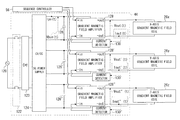
- FIG. 4 is a block diagram showing an example of a configuration of a gradient magnetic field power supply 44 in FIG. 1 ;
- FIG. 5 is a circuit diagram showing an example of an equivalent circuit model of the gradient magnetic field generation system used in the calculation to judge whether an imaging sequence is practicable or not;
- FIG. 6 is a graph schematically showing measurements of frequency characteristics of the real part Re ⁇ Z ⁇ of the impedance Z of a gradient magnetic field coil
- FIG. 7 is a graph schematically showing measurements of frequency characteristics of Im ⁇ Z ⁇ / ⁇ , which is the imaginary part Im ⁇ Z ⁇ of the impedance Z of the gradient magnetic field coil divided by an angular frequency ⁇ ;
- FIG. 8 is a schematic diagram showing an example of data of MR signals immediately before transformation into k-space data, in the case where the number of matrix elements in the phase encode direction is 256 and the number of matrix elements in the frequency encode direction is 256;
- FIG. 9 is a schematic diagram showing an example of the gradient magnetic field waveform in the readout direction in EPI;
- FIG. 10 is a schematic diagram showing an example of the waveform of the output voltage Vout(t) shown in FIG. 4 that is simplified on the assumption that the output voltage Vout(t) complies with the formula (33);
- FIG. 11 is a schematic diagram showing an example of the waveform of the output voltage Vout(t) shown in FIG. 4 calculated based on the equivalent circuit model shown in FIG. 5 ;
- FIG. 12 is a schematic diagram showing an example of a display screen for setting the conditions of an imaging sequence before the first to third judgment algorithms are performed;
- FIG. 13 is a schematic diagram showing an example of a display screen for setting the conditions of the imaging sequence, in a case where it is judged according to at least one of the first to third judgment algorithms that the imaging sequence is impracticable;
- FIG. 14 is a flowchart illustrating a flow of a process performed by the MRI apparatus of the first embodiment
- FIG. 15 is a block diagram showing the gradient magnetic field power supply and the gradient magnetic field coils, in the case where line filters are taken into consideration;
- FIG. 16 is a circuit diagram showing another example of the equivalent circuit model of the gradient magnetic field generation system used in the calculation for judging whether an imaging sequence is practicable or not;
- FIG. 17 is a circuit diagram showing another example of the equivalent circuit model of the gradient magnetic field generation system used in the calculation for judging whether the imaging sequence is practicable or not;
- FIG. 18 is a functional block diagram showing the computer in the MRI apparatus according to the second embodiment.
- FIG. 19 is a schematic diagram showing a concept of conventional regridding processing
- FIG. 20 is a schematic diagram showing a concept of a calculation method for a gradient magnetic field waveform according to the second embodiment
- FIG. 21 is a schematic diagram for illustrating an example of an imaging sequence of spin echo EPI
- FIG. 22 is a conceptual diagram showing that MR signals sampled at equal time intervals in a region where the gradient magnetic field Gro in the readout direction is nonlinear are placed at unequal intervals in the k-space;
- FIG. 23 is a schematic diagram showing a concept of the first method of the regridding processing
- FIG. 24 is a schematic diagram showing a concept of the second method of the regridding processing
- FIG. 25 is a flowchart illustrating an example of a flow of a process performed by the MRI apparatus of the second embodiment
- FIG. 26 is a flowchart illustrating an example of a flow of a process performed by the MRI apparatus of the third embodiment
- FIG. 27 is a schematic diagram for illustrating an example of the method of correcting a parameter concerning the gradient magnetic field Gss in the slice selection direction in EPI;
- FIG. 28 is a schematic diagram for illustrating an example of the method of correcting a parameter, concerning the gradient magnetic field Gpe in the phase encode direction in EPI;
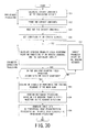
- FIG. 29 is a flowchart illustrating an example of a flow of a process performed by the MRI apparatus of the fourth embodiment.
- FIG. 30 is a flowchart illustrating an example of a flow of a process performed by the MRI apparatus of the fifth embodiment.
- a magnetic resonance imaging apparatus and its control device include a condition setting unit and a judging unit.
- the condition setting unit sets an imaging sequence performed by the magnetic resonance imaging apparatus, based on conditions of the imaging sequence.
- the judging unit calculates a value of electric current supplied to a gradient magnetic field coil of the magnetic resonance imaging apparatus based on the conditions of the imaging sequence.
- the judging unit calculates a value of voltage applied to the gradient magnetic field coil based on a mutual inductance by which the gradient magnetic field coil causes mutual induction, in such a manner that electric current flowing the gradient magnetic field coil becomes equal to the value of an electric current calculated. Then, the judging unit judges whether the imaging sequence is practicable or not, based on the value of voltage.
- a magnetic resonance imaging apparatus applies a gradient magnetic field to an imaging region, generates k-space data including a plurality of matrix elements by sampling a nuclear magnetic resonance signal acquired from the imaging region, and reconstructs image data based on the k-space data.
- This magnetic resonance imaging apparatus includes a gradient magnetic field power supply, a gradient magnetic field calculating unit, and a regridding processing unit.
- the gradient magnetic field power supply applies the gradient magnetic field to the imaging region, by supplying gradient magnetic field current to a gradient magnetic field coil under an imaging sequence;
- the gradient magnetic field calculating unit calculates a waveform of the gradient magnetic field current based on conditions of the imaging sequence.
- the gradient magnetic field calculating unit calculates a waveform of a gradient magnetic field in a readout direction, based on a mutual inductance by which the gradient magnetic field coil causes mutual induction and the waveform of the gradient magnetic field current.
- the regridding processing unit generates or rearranges the k-space data by sampling at unequally-spaced intervals, in such a manner that a part of the nuclear magnetic resonance signal acquired during a time span in which a time integral value of intensity of the gradient magnetic field in a readout direction is non-linear and each time integral value up to a sampling period corresponding to each of the matrix elements becomes equally-spaced.
- a magnetic resonance imaging apparatus applies a gradient magnetic field to an imaging region, reconstructs image data based on a nuclear magnetic resonance signal acquired from the imaging region.
- This magnetic resonance imaging apparatus includes the gradient magnetic field power supply which is similar to the above (2), the gradient magnetic field calculating unit which is similar to the above (2) and a waveform correcting unit.
- the waveform correcting unit corrects at least one of the conditions of the imaging sequence before performance of the imaging sequence, in such a manner that the waveform of the gradient magnetic field in a readout direction becomes closer to a target waveform for the gradient magnetic field in a readout direction, if the waveform of the gradient magnetic field in a readout direction calculated by the gradient magnetic field calculating unit is different from the target waveform.
- FIG. 1 is a block diagram showing general structure of the MRI apparatus 20 A according to the first embodiment.
- the MRI apparatus 20 A includes a cylinder-shaped static magnetic field magnet 22 for generating a static magnetic field, a cylinder-shaped shim coil 24 coaxially-arranged inside the static magnetic field magnet 22 , a gradient magnetic field coil 26 , RF coils 28 , a control device 30 , and a bed 32 for placing an object (e.g. a patient) QQ on it.
- an apparatus coordinate system whose X axis, a Y axis and a Z axis are perpendicular to each other, is defined as follows. Firstly, the direction of an axis of the static magnetic field magnet 22 and the shim coil 24 is aligned with the direction which is perpendicular to the vertical direction, and the direction of the axis of the static magnetic field magnet 22 and the shim coil 24 is defined as the Z axis direction.
- the vertical direction is the same as the Y axis direction.
- the bed 32 is disposed in such a position that the direction of the normal line of the table plane thereof on which an object is put is the same as the Y axis direction.
- the control device 30 includes, for example, a static magnetic field power supply 40 , a shim coil power supply 42 , a gradient magnetic field power supply 44 , an RF transmitter 46 , an RF receiver 48 , a sequence controller 56 and a computer 58 .
- the gradient magnetic field power supply 44 includes an X axis gradient magnetic field power supply 44 x , a Y axis gradient magnetic field power supply 44 y and a Z axis gradient magnetic field power supply 44 z.
- the computer 58 includes an operation device 60 , an input device 62 , a display device 64 and a storage device 66 .
- the static magnetic field magnet 22 is electrically connected to the static magnetic field power supply 40 and generates a static magnetic field in an imaging space by using electric current supplied from the static magnetic field power supply 40 .
- the aforementioned imaging space means, for example, a space in the gantry 21 (see FIG. 2 ) in which an object QQ is placed and to which a static magnetic field is applied.
- FIG. 1 does not show the gantry 21 itself, but shows the components of the gantry 21 such as the static magnetic field magnet 22 .
- the shim coil 24 is electrically connected to the shim coil power supply 42 and uniforms the static magnetic field with the electric current supplied from the shim coil power supply 42 .
- the static magnetic field magnet 22 includes a superconductivity coil in many cases.
- the static magnetic field magnet 22 gets electric current from the static magnetic field power supply 40 at excitation. However, once excitation has been made, the static magnetic field magnet 22 is usually isolated from the static magnetic field power supply 40 .
- the static magnetic field magnet 22 may include a permanent magnet which makes the static magnetic field power supply 40 unnecessary.
- the gradient magnetic field coil 26 includes an X axis gradient magnetic field coil 26 x , a Y axis gradient magnetic field coil 26 y and a Z axis gradient magnetic field coil 26 z .
- Each of the X axis gradient magnetic field coil 26 x , the Y axis gradient magnetic field coil 26 y and the Z axis gradient magnetic field coil 26 z is cylinder-shaped and arranged inside the static magnetic field magnet 22 .
- the X axis gradient magnetic field coil 26 x , the Y axis gradient magnetic field coil 26 y and the Z axis gradient magnetic field coil 26 z are electrically connected to the X axis gradient magnetic field power supply 44 x , the Y axis gradient magnetic field power supply 44 y and the Z axis gradient magnetic field power supply 44 z of the gradient magnetic field power supply 44 , respectively.
- the X axis gradient magnetic field power supply 44 x , the Y axis gradient magnetic field power supply 44 y and the Z axis gradient magnetic field power supply 44 z supply electric current to the X axis gradient magnetic field coil 26 x , the Y axis gradient magnetic field coil 26 y and the Z axis gradient magnetic field coil 26 z respectively, so as to generate a gradient magnetic field Gx in the X axis direction, a gradient magnetic field Gy in the Y axis direction and a gradient magnetic field Gz in the Z axis direction in the imaging region.
- directions of a gradient magnetic field Gss in a slice selection direction, a gradient magnetic field Gpe in a phase encode direction and a gradient magnetic field Gro in a readout (frequency encode) direction can be arbitrarily set as logical axes, by combining gradient magnetic fields Gx, Gy and Gz in the X axis, Y axis and Z axis directions as three physical axes.
- the gradient magnetic fields Gss, Gpe and Gro in the slice selection direction, the phase encode direction and the readout direction are superimposed on the static magnetic field.
- the aforementioned imaging region means, for example, at least a part of an acquisition range of MR signals used to generate one image or one set of images, which becomes an image.
- the imaging region is defined as a part of the imaging space in terms of range and position by an apparatus coordinate system, for example.
- the entire acquisition range of MR signals becomes an image, i.e. the imaging region and the acquisition range of MR signals agree with each other.
- the imaging region and the acquisition range of MR signals do not agree with each other.
- the imaging region is a part of the acquisition range of MR signals.
- the one image or one set of images may be a two-dimensional image or a three-dimensional image.
- one set of images means, for example, a plurality of images when MR signals of the plurality of images are acquired in a lump in one pulse sequence such as multi-slice imaging.
- the RF transmitter 46 generates RF pulses (RF pulse electric current) in accordance with control information provided from the sequence controller 56 , and outputs the generated RF pulses to the transmission RF coil 28 .
- the RF coils 28 include whole body coil built in the gantry 21 for transmission and reception of RF pulses and local coils arranged around the bed 32 or the object QQ for reception of RF pulses.
- the transmission RF coil 28 transmits an RF pulse given from the RF transmitter 46 to the object QQ.
- the reception RF coil 28 receives an MR signal generated due to excited nuclear spin inside the object QQ by the RF pulse and this MR signal is detected by the RF receiver 48 .
- the RF receiver 48 generates raw data which are digitized complex number data obtained by performing A/D (analogue to digital) conversion after performing predetermined signal processing such as preamplification, intermediate-frequency conversion, phase detection, low-frequency amplification and filtering on the detected MR signal.
- the RF receiver inputs the generated raw data to the sequence controller 56 .
- the operation device 60 performs system control of the MRI apparatus 20 in imaging operation, and its function will be explained later with FIG. 3 .
- the sequence controller 56 storages control information needed in order to make the gradient magnetic field power supply 44 , the RF transmitter 46 and the RF receiver 48 drive, under the control by the operation device 60 .
- the aforementioned control information includes, for example, sequence information describing operation control information such as intensity, impression period and impression timing of the pulse electric current which should be impressed to the gradient magnetic field power supply 44 .
- the sequence controller 56 generates the gradient magnetic fields Gx, Gy and Gz in the X axis, Y axis and Z axis directions and RF pulses, by driving the gradient magnetic field power supply 44 , the RF transmitter 46 and the RF receiver 48 according to a predetermined sequence stored. Additionally, the sequence controller 56 receives the raw data of an MR signal inputted from the RF receiver 48 , and input the raw data to the operation device 60 .
- FIG. 2 is a schematic perspective view showing an arrangement of temperature sensors in the gantry 21 .
- the static magnetic field magnet 22 In the gantry 21 , the static magnetic field magnet 22 , the shim coil 24 , the gradient magnetic field coil 26 having a cylindrical shape shown in FIG. 1 are arranged (not shown in FIG. 2 for the sake of simplicity).
- the gradient magnetic field coil 26 has a multilayer structure that comprises, in ascending order of the distance from the center, a layer of an X axis gradient magnetic field coil 26 x , a layer of a Y axis gradient magnetic field coil 26 y , a layer of a Z axis gradient magnetic field coil 26 z and a cooling layer (not shown), for example, molded to form a cylindrical shape.
- the cooling layer is a structure including a cooling tube arranging layer and a shim tray arranging layer.
- temperature sensors 70 x 1 , 70 x 2 and 70 x 3 are embedded at equal intervals in the Z axis direction in the apparatus coordinate system.
- temperature sensors 70 y 1 , 70 y 2 and 70 y 3 are embedded at equal intervals in the Z axis direction in the apparatus coordinate system.
- temperature sensors 70 z 1 , 70 z 2 and 70 z 3 are embedded at equal intervals in the Z axis direction in the apparatus coordinate system.
- the temperature sensors 70 x 1 to 70 x 3 detect the temperature of the X axis gradient magnetic field coil 26 x at their respective positions and input (transmit) the detected temperatures to a judging unit 102 (see FIG. 3 , described later) via the sequence controller 56 .
- the temperature sensors 70 y 1 to 70 y 3 detect the temperature of the Y axis gradient magnetic field coil 26 y at their respective positions and input the detected temperatures to the judging unit 102 .
- the temperature sensors 70 z 1 to 70 z 3 detect the temperature of the Z axis gradient magnetic field coil 26 z at their respective positions and input the detected temperatures to the judging unit 102 .
- the arrangement of the temperature sensors 70 x 1 to 70 x 3 , 70 y 1 to 70 y 3 and 70 z 1 to 70 z 3 is just an example.
- four or more temperature sensors may be embedded, and the judging unit 102 may calculate the maximum of the temperatures detected by the sensors.
- one or two temperature sensors may be embedded in each of the layers of the X axis gradient magnetic field coil 26 x , the Y axis gradient magnetic field coil 26 y and the Z axis gradient magnetic field coils 26 z.
- the temperature sensors 70 x 1 to 70 x 3 , 70 y 1 to 70 y 3 and 70 z 1 to 70 z 3 may be an infrared radiation thermometer, or a thermistor, a thermocouple or the like that substantially directly measures the temperature of the X axis gradient magnetic field coil 26 x , the Y axis gradient magnetic field coil 26 y and the Z axis gradient magnetic field coils 26 z.
- the infrared radiation thermometer can measure the temperature of the object QQ without coming into contact with the object QQ.
- the infrared radiation thermometer has an advantage that it can measure the temperature in a shorter time than “measuring methods that require the temperatures of the measurement target and the temperature sensor to be equal to each other as a result of heat conduction”.
- the operation device 60 of the computer 58 provides various functions, including control of the sequence controller 56 and control of the whole system of the MRI apparatus 20 A, according to a program stored in the storage device 66 . These various functions can also be provided by a particular circuit provided in the MRI apparatus 20 A.
- components including the gantry 21 ) other than those of the control device 30 are installed in an examination room, and the components of the control device 30 are installed in a different room (a machine room, for example).
- a different room a machine room, for example.
- embodiments of the present invention are not limited to this way of installation.
- the RF receiver 48 may be disposed in the gantry 21 .
- the RF receiver 48 may be disposed in the vicinity of the receiving RF coil 28 in the gantry 21 , convert an analog signal into a digital signal (and further into an optical signal) and transmit the resulting signal to the sequence controller 56 in the machine room. In this case, interference with unwanted noise can be reduced.
- FIG. 3 is a functional block diagram of the computer 58 shown in FIG. 1 .
- the operation device 60 of the computer 58 includes an MPU (Micro Processor Unit) 86 , a system bus 88 , an image reconstruction unit 90 , an image database 94 , an image processing unit 96 , a display controlling unit 98 , a condition setting unit 100 , and a judging unit 102 .
- MPU Micro Processor Unit
- the MPU 86 performs system control of the MRI apparatus 20 A in setting of conditions of an imaging sequence, imaging operation and image display after imaging through interconnection such as the system bus 88 .
- the MPU 86 controls the display controlling unit 98 and displays screen information for setting conditions of an imaging sequence on the display device 64 .
- the input device 62 is, for example, an input tool such as a keyboard and a mouse, and provides a user with a function to set conditions of an imaging sequence and image processing conditions.
- the display device 64 is, for example, a display equipment including a liquid crystal display.
- a user interface is composed of the input device 62 and the display device 64 .
- the image reconstruction unit 90 includes a k-space database 92 inside.
- the image reconstruction unit 90 arranges the raw data of MR signals inputted from the sequence controller 56 in the k-space (frequency-space) formed in the k-space database 92 as k-space data.
- the image reconstruction unit 90 generates image data of each slice of the object QQ by performing image reconstruction processing including such as 2-dimensional Fourier transformation.
- the image reconstruction unit 90 stores the generated image data in the image database 94 .
- the image processing unit 96 takes in the image data from the image database 94 , performs predetermined image processing on them, and stores the image data after the image processing in the storage device 66 as image data for display.
- the storage device 66 stores the image data for display after adding accompanying information such as imaging conditions used for generating the image data for display and information of the object QQ (patient information) to the image data for display.
- the display controlling unit 98 displays a screen for setting conditions of an imaging sequence and an image indicated by generated image data through imaging on the display device 64 , under control of the MPU 86 .
- the condition setting unit 100 sets a condition for an imaging sequence based on information inputted via the input device 62 . If the judging unit 102 judges that the set imaging sequence is impracticable, the condition setting unit 100 calculates a correction candidate for the conditions of the imaging sequence to make the imaging sequence practicable.
- the judging unit 102 judges whether or not the imaging sequence set by the condition setting unit 100 is practicable according to the first to third judgment algorithms.
- the judging unit 102 judges that the imaging sequence is practicable, only if neither of the first to third judgment algorithms has judged that the imaging sequence is impracticable.
- the first to third judgment algorithms are to make the judgment of whether the imaging sequence is practicable or not through calculation based on an equivalent circuit model of a gradient magnetic field generation system.
- FIG. 4 is a block diagram showing an example of a configuration of a gradient magnetic field power supply 44 .
- the gradient magnetic field power supply 44 has a breaker (circuit breaker) 122 , a rectifier 123 , a direct-current power supply 124 , electrolyte capacitors 126 , 126 ′ and 126 ′′, gradient magnetic field amplifiers 128 , 128 ′ and 128 ′′, and current detectors 130 , 130 ′ and 130 ′′.
- the X axis gradient magnetic field power supply 44 x , the Y axis gradient magnetic field power supply 44 y and the Z axis gradient magnetic field power supply 44 z shown in FIG. 1 share the breaker 122 , the rectifier 123 and the direct-current power supply 124 that has CV/CC characteristics.
- the X axis gradient magnetic field power supply 44 x shown in FIG. 1 corresponds to the breaker 122 , the rectifier 123 , the direct-current power supply 124 , the electrolyte capacitor 126 , the gradient magnetic field amplifier 128 and the current detector 130 .
- the direct-current power supply 124 having CV/CC characteristics is a power supply that outputs a constant voltage when the load is light and, when the load is heavy and electric current equal to or higher than a certain level needs to be supplied, supplies constant electric current to the load rather than outputting the needed current. That is, “CV” is an abbreviation of constant voltage, and “CC” is an abbreviation of constant current.
- the Y axis gradient magnetic field power supply 44 y shown in FIG. 1 corresponds to the breaker 122 , the rectifier 123 , the direct-current power supply 124 , the electrolyte capacitor 126 ′, the gradient magnetic field amplifier 128 ′ and the current detector 130 ′.
- the Z axis gradient magnetic field power supply 44 z shown in FIG. 1 corresponds to the breaker 122 , the rectifier 123 , the direct-current power supply 124 , the electrolyte capacitor 126 ′′, the gradient magnetic field amplifier 128 ′′ and the current detector 130 ′′.
- the breaker 122 electrically disconnects an external alternating-current power supply 120 and the rectifier 123 from each other, when the output current from the alternating-current power supply 120 exceeds a rated current value.
- the rectifier 123 converts the alternating-current power supplied from the alternating-current power supply 120 into a direct-current power, and supplies the direct-current power to the direct-current power supply 124 .
- the direct-current power supply 124 charges the electrolyte capacitors 126 , 126 ′ and 126 ′′ with the direct current supplied via the rectifier 123 and supplies the direct current to the gradient magnetic field amplifiers 128 , 128 ′ and 128 ′′.
- the direct-current power supply 124 operates as a constant voltage source, when the load on the side of the gradient magnetic field amplifiers 128 , 128 ′ and 128 ′′ is light.
- the direct-current power supply 124 operates as a constant current source, when the load is heavy.
- Each of the gradient magnetic field amplifiers 128 , 128 ′ and 128 ′′ has a positive-side input terminal (+IN in the drawing), a negative-side input terminal ( ⁇ IN in the drawing), a positive-side output terminal (+OUT in the drawing) and a negative-side output terminal ( ⁇ OUT in the drawing).
- Each of the gradient magnetic field amplifiers 128 , 128 ′ and 128 ′′ receives the power from the direct-current power supply 124 and receives a control signal (voltage signal) from the sequence controller 56 at the positive-side input terminal.
- the control signals inputted from the sequence controller 56 to the gradient magnetic field amplifiers 128 , 128 ′ and 128 ′′ have waveforms similar to ideal waveforms of the magnetic fields to be generated by the X axis gradient magnetic field coil 26 x , the Y axis gradient magnetic field coil 26 y and the Z axis gradient magnetic field coil 26 z according to the imaging sequence, respectively.
- the current detectors 130 , 130 ′ and 130 ′′ detects the values of each electric current flowing into the negative-side output terminals of the gradient magnetic field amplifiers 128 , 128 ′ and 128 ′′, respectively, and the magnitudes of the detected electric current are equal to the magnitudes of the current outputted from the positive-side output terminals of the gradient magnetic field amplifiers 128 , 128 ′ and 128 ′′.
- each electric current outputted from the positive-side output terminals of the gradient magnetic field amplifiers 128 , 128 ′ and 128 ′′ are fed back to the negative-side output terminals of the gradient magnetic field amplifiers 128 , 128 ′ and 128 ′′ through the gradient magnetic field coils 26 x , 26 y and 26 z , respectively.
- the current detectors 130 , 130 ′ and 130 ′′ generate voltage signals indicative of the values of the each detected electric current, and input the generated voltage signals to the negative-side input terminals of the gradient magnetic field amplifiers 128 , 128 ′ and 128 ′′, respectively.
- the gradient magnetic field amplifiers 128 , 128 ′ and 128 ′′ each operate as a current source that outputs electric current, in such a manner that the error signal between the positive-side input terminal and the negative-side input terminal is 0.
- each output electric current of the gradient magnetic field amplifiers 128 , 128 ′ and 128 ′′ are negatively fed back by the current detectors 130 , 130 ′ and 130 ′′.
- the feedback control occurs, in such a manner that each electric current proportional to the voltages inputted to the positive-side input terminals of the gradient magnetic field amplifiers 128 , 128 ′ and 128 ′′ are outputted from the respective positive-side output terminals.
- FIG. 5 is a circuit diagram showing an example of an equivalent circuit model of the gradient magnetic field generation system used in the calculation for the judging unit 102 to judge whether the imaging sequence is practicable or not.
- the gradient magnetic field generation system refers to the whole of the components involved in generation of the gradient magnetic field, including the gradient magnetic field power supply 44 , the gradient magnetic field coil 26 and the sequence controller 56 shown in FIG. 1 .
- the judging unit 102 judges by calculation whether the imaging sequence is practicable or not on the assumption that the gradient magnetic field generation system has the circuit configuration shown in FIG. 5 . That is, the actual gradient magnetic field generation system of the MRI apparatus 20 A has the configuration shown in FIG. 4 , which differs from the circuit configuration shown in FIG. 5 .
- an equivalent circuit model 140 x has, on the primary side, the X axis gradient magnetic field power supply 44 x , a resistor 26 x R that corresponds to the resistance component of the X axis gradient magnetic field coil 26 x , and a coil 26 x L that corresponds to the inductance component of the X axis gradient magnetic field coil 26 x , which are connected to each other in series.
- the equivalent circuit model 140 x further has a series circuit of a resistor 141 R and a coil 141 L as a first secondary-side circuit.
- the equivalent circuit model 140 x further has a series circuit of a resistor 142 and a coil 142 L as a second secondary-side circuit.
- the coil 26 x L and the coil 141 L are electromagnetically coupled to each other.
- the coil 26 x L and the coil 142 L are also electromagnetically coupled to each other.
- the impedances of the X axis gradient magnetic field coil 26 x , the Y axis gradient magnetic field coil 26 y and the Z axis gradient magnetic field coil 26 z do not simply increase as in a simple model in which the impedance is expressed by the sum of one resistance component and one inductance component.
- the electric current density is highest at the surface of the conductor and decreases as the distance from the surface increases.
- the electric current is more highly concentrated at the surface, because of the skin effect, and therefore, the alternating-current resistance of the conductor increases.
- the term involving the resistance value of the resistor 26 x R of the X axis gradient magnetic field coil 26 x in the polynomial expressing the impedance of the gradient magnetic field generation system also desirably varies depending on the frequency.
- the actual gradient magnetic field generation system may include a choke coil that cuts off high frequency electric current at a predetermined frequency or higher.
- a choke coil that cuts off high frequency electric current at a predetermined frequency or higher.
- the equivalent circuit model 140 x shown in FIG. 5 is just an example of the equivalent circuit models described above, and the equivalent circuit model is not limited to the configuration shown in FIG. 5 (see FIGS. 16 and 17 described later).
- the series circuit of the resistor 141 R and the coil 141 L and the series circuit of the resistor 142 R and the coil 142 L are actually existing components that correspond to the mutual inductance component, the resistance component or the like involved in the magnetic field generated by the eddy current, the skin effect or the like.
- the series circuit of the resistor 141 R and the coil 141 L is regarded as a “virtual coil” different from the gradient magnetic field coil 26 .
- the resistance value of the resistor 141 R is regarded as the resistance component of the virtual coil
- the self-inductance value of the coil 141 L is regarded as the self-inductance value of the virtual coil.
- the series circuit of the resistor 141 R and the coil 141 L is not a non-existing component but is an expression of the actually existing mutual inductance component or the like in the equivalent circuit.
- the resistance values of the resistors 26 x R, 141 R and 142 R are denoted by Rload, R 1 and R 2 , respectively.
- the self-inductance values of the coils 26 x L, 141 L and 142 L are denoted by Lload, L 1 and L 2 , respectively.
- the mutual inductance value of the coils 26 x L and 141 L is denoted by M 1 .
- the mutual inductance value of the coils 26 x L and 142 L is denoted by M 2 .
- Iout(t) The value of the electric current flowing in the primary-side circuit in the direction of the arrow in FIG. 5 is denoted by Iout(t).
- I 1 (t) The value of the electric current flowing in the first secondary-side circuit in the direction of the arrow in FIG. 5 is denoted by I 1 (t).
- I 2 (t) The value of the electric current flowing in the second secondary-side circuit in the direction of the arrow in FIG. 5 is denoted by I 2 (t).
- Vout(t) The value of the voltage across “the coil 26 x L and the resistor 26 x R” is denoted by Vout(t), on the assumption that the direction of the arrow in FIG. 5 is the positive direction.
- M 1 in the formulas (1) to (3) is expressed by the following formula (4)
- M 2 in the formulas (1) to (3) is expressed by the following formula (5).
- M 1 K 1 ⁇ square root over (L load ⁇ L 1 ) ⁇
- M 2 K 2 ⁇ square root over (L load ⁇ L 2 ) ⁇ (5)
- K 1 in the formula (4) denotes a coupling coefficient of the coils 26 x L and 141 L
- K 2 in the formula (5) denotes a coupling coefficient of the coils 26 x L and 142 L.
- the imaginary unit is denoted by j. That is, j squared equals to ⁇ 1.
- I 1 ⁇ ( t ) - j ⁇ ⁇ ⁇ M 1 R 1 + j ⁇ ⁇ ⁇ L 1 ⁇ Iout ⁇ ( t ) ( 6 )
- I 2 ⁇ ( t ) - j ⁇ ⁇ ⁇ M 2 R 2 + j ⁇ ⁇ ⁇ L 2 ⁇ Iout ⁇ ( t ) ( 7 )
- the impedance of the X axis gradient magnetic field coil 26 x viewed from the X axis gradient magnetic field power supply 44 x is denoted by Z. If both sides of the formula (1) are divided by Iout(t), the time differential d/dt is replaced with j ⁇ , and the formulas (6) and (7) are substituted into the formula (1), the impedance Z is expressed by the following formula (8).
- the real part Re ⁇ Z ⁇ and the imaginary part Im ⁇ Z ⁇ of the impedance Z viewed from the X axis gradient magnetic field power supply 44 x are expressed by the following formulas (9) and (10), respectively.
- Circuit constants A, B, C and D in the formulas (9) and (10) are expressed by the following formulas (11), (12), (13) and (14), respectively.
- A M 1 2 R 1 ( 11 )
- B L 1 2 R 1 2 ( 12 )
- C M 2 2 R 2 ( 13 )
- D L 2 2 R 2 2 ( 14 )
- FIG. 6 is a graph schematically showing measurements of frequency characteristics of the real part Re ⁇ Z ⁇ of the impedance Z of the X axis gradient magnetic field coil 26 x .
- the horizontal axis indicates frequency
- the vertical axis indicates the real part Re ⁇ Z ⁇ of the impedance Z.
- FIG. 7 is a graph schematically showing measurements of frequency characteristics of Im ⁇ Z ⁇ / ⁇ , which is the imaginary part Im ⁇ Z ⁇ of the impedance Z of the X axis gradient magnetic field coil 26 x divided by ⁇ .
- the horizontal axis indicates frequency
- the vertical axis indicates Im ⁇ Z ⁇ / ⁇ .
- the resistance value Rload in the formula (9) and the like is preliminarily determined by measuring the voltage across the X axis gradient magnetic field coil 26 x in the case where a direct current is passed through the X axis gradient magnetic field coil 26 x , and is preliminarily stored in the judging unit 102 .
- the measurement can be achieved with an LCR meter, for example (“L” in LCR means inductance, “C” means capacitance, and “R” means resistance).
- the self-inductance value Lload in the formula (10) and the like can be calculated from measurements of the magnetic flux generated by the X axis gradient magnetic field coil 26 x when a direct current is passed through the X axis gradient magnetic field coil 26 x , for example.
- the self-inductance value Lload may be determined by measurement with the LCR meter at a low frequency (1 to 10 Hertz, for example) at which the self-inductance value is not affected by the secondary side in the equivalent circuit model 140 x.
- a theoretical value of the self-inductance value Lload may be calculated from the shape (the way of winding of the coil), the material or the like of the X axis gradient magnetic field coil 26 x and used.
- the self-inductance value preliminarily determined in this way is preliminarily stored in the judging unit 102 .
- calculated values and measurements of the phase difference between the real part Re ⁇ Z ⁇ and the imaginary part Im ⁇ Z ⁇ of the impedance Z may be used for the fittings.
- the mutual inductances M 1 and M 2 are determined according to the formulas (4) and (5), and the circuit constants A, B, C and D are determined according to the formulas (11) to (14).
- the inductance values Rload and Lload and the circuit constants A, B, C and D determined as described above are preliminarily stored in the judging unit 102 .
- the real part Re ⁇ Z ⁇ and the imaginary part Im ⁇ Z ⁇ of the impedance Z at any frequency can be calculated according to the formulas (9) and (10).
- the electric current I 1 (t) and the electric current I 2 (t) are accidental electric current occurring in the equivalent circuit model 140 x that is induced by the output current Iout(t) of the actual gradient magnetic field generation system.
- both sides of the formula (23) are differentiated with respect to time to obtain the following formula (24), and both sides of the formula (16) are multiplied by M 1 ⁇ (L 1 ⁇ R 2 ⁇ L 2 ⁇ R 1 ) to obtain the following formula (25).
- the following formula (26) is obtained.
- the output electric current Iout(t) outputted from the X axis gradient magnetic field power supply 44 x that is, the electric current flowing through the X axis gradient magnetic field coil 26 x , is determined by the conditions of the imaging sequence.
- the gradient magnetic field waveform of the X axis gradient magnetic field Gx to be generated is determined, and the gradient magnetic field waveform of the X axis gradient magnetic field Gx is determined by the waveform of the electric current flowing through the X axis gradient magnetic field coil 26 x.
- the formula (27) is the second order time differential equation of the output voltage Vout(t).
- the output voltage Vout(t) required to pass the output electric current Iout(t) through the X axis gradient magnetic field coil 26 x can be calculated by solving the equation.
- the output power required to pass the output electric current Iout(t) through the X axis gradient magnetic field coil 26 x can be underestimated. In such a case, the output voltage can be inadequate during the imaging sequence.
- the output voltage Vout(t), and therefore the output power, required to pass the output electric current Iout(t) through the X axis gradient magnetic field coil 26 x can be accurately calculated.
- the voltage can be prevented from being inadequate (insufficient) during the imaging sequence.
- a power consumption Pxcoil(t) of the X axis gradient magnetic field coil 26 x can be calculated according to the following formula (28).
- Px coil( t ) I out( t ) ⁇ V out( t ) (28)
- the amount ⁇ Heat of heat generated by the X axis gradient magnetic field coil 26 x can be calculated as a time integral of the power consumption Pxcoil(t) over a period from the start time to the end time of the imaging sequence.
- the thermal resistance value of the X axis gradient magnetic field coil 26 x is denoted by RHX
- the thermal resistance value RHX of the X axis gradient magnetic field coil 26 x is a measured value, for example, and is preliminarily stored in the judging unit 102 .
- a constant direct current is passed through the X axis gradient magnetic field coil 26 x , and the voltage across the X axis gradient magnetic field coil 26 x is measured, thereby calculating the power applied to the X axis gradient magnetic field coil 26 x.
- the increase in temperature of the X axis gradient magnetic field coil 26 x in a period from a point in time immediately before application of the direct current to a point in time immediately after application of the direct current is measured with the temperature sensors 70 x 1 to 70 x 3 . Once the power applied to the X axis gradient magnetic field coil 26 x and the temperature increase provided thereby are determined by this measurement, the thermal resistance value RHX can be calculated.
- the temperature Tempx of the X axis gradient magnetic field coil 26 x immediately after the imaging sequence is performed can be calculated by adding the temperature increase ⁇ Tempx calculated based on the equivalent circuit model 140 x to the measured temperature of the X axis gradient magnetic field coil 26 x immediately before the imaging sequence is performed.
- the judging unit 102 preliminarily stores the formulas (1) to (29) described above and the circuit constants (A, B and the like) found in these formulas. Therefore, if the temperature of the X axis gradient magnetic field coil 26 x immediately after the imaging sequence is performed is higher than a preset threshold, the judging unit 102 judges that the imaging sequence is impracticable.
- the judging unit 102 calculates the temperature of the Y axis gradient magnetic field coil 26 y immediately after the imaging sequence is performed in the same manner, and judges that the imaging sequence is impracticable if the calculated temperature is higher than a threshold.
- the judging unit 102 calculates the temperature of the Z axis gradient magnetic field coil 26 z immediately after the imaging sequence is performed in the same manner, and judges that the imaging sequence is impracticable if the calculated temperature is higher than a threshold.
- the judging unit 102 judges that the imaging sequence is practicable.
- the regridding processing refers to rearrangement of k-space data arranged in a matrix (matrix data) in a k-space. In the following, the regridding processing will be described in detail.
- the electric current sensitivity of the coil 26 x L which is a main coil, is denoted by ⁇
- the current sensitivity of the coil 141 L is denoted by ⁇
- the current sensitivity of the coil 142 L is denoted by ⁇ .
- the electric current sensitivity is a constant obtained by dividing the intensity (Tesla/meter) of the gradient magnetic field generated by electric current flowing through the coil by the value (ampere) of the current flowing through the coil.
- the waveform of the X axis gradient magnetic field Gx(t) which is the sum of magnetic fields including the magnetic field induced by the eddy current, can be calculated as a waveform of a sum magnetic field as expressed by the following formula.
- Gx ( t ) ⁇ I out( t )+ ⁇ I 1 ( t )+ ⁇ I 2 ( t ) (30)
- the second and third terms in the right side of the formula (30) are examples of the waveforms of the magnetic fields generated by the coils 141 L and 142 L (virtual magnetic field waveforms).
- the output electric current Iout(t) flowing through the X axis gradient magnetic field coil 26 x is determined by the conditions of the imaging sequence.
- the electric current I 1 (t) flowing through the coil 141 L on the secondary side and the electric current I 2 (t) flowing through the coil 142 L can be determined according to the formula (30).
- Both the initial values of the electric current I 1 (t) and the electric current I 2 (t) can be zero, if it is assumed that a sufficient time has elapsed after the end of the preceding imaging sequence, for example.
- the formula (30) contains no unknown quantity, and the waveform of the magnetic field Gx(t) can be calculated.
- the accuracy of the regridding processing in reconstruction is improved by changing the intervals of reception sampling based on the waveform of the magnetic field Gx(t) expressed by the formula (30). In the following, this example will be described in more detail.
- FIG. 8 is a schematic diagram showing an example of data of MR signals immediately before transformation into k-space data, in the case where the number of matrix elements in the phase encode direction is 256 and the number of matrix elements in the frequency encode direction is 256.
- TR denotes repetition time
- Ts on the horizontal axis denotes sampling time
- the vertical axis indicates phase encode step
- the 256 lines of MR signals acquired by changing the position in the phase encode direction 256 times are arranged for each encode step as shown in FIG. 8 after the cosine function or sine function of the carrier frequency is subtracted from each MR signal.
- the sampling time Ts of each MR signal on the horizontal axis in FIG. 8 is equally divided by 256, and the intensity of the MR signal for each resulting time ⁇ Ts is regarded as a matrix value of the matrix element.
- FIG. 9 is a schematic diagram showing an example of the gradient magnetic field waveform in the readout direction in EPI.
- the vertical axis indicates the amplitude (intensity) of the magnetic field in the readout direction
- the horizontal axis indicates elapsed time t.
- the actual inversion of the gradient magnetic field in the readout direction is not an instantaneous inversion of the polarity of the amplitude of the magnetic field with a slop that is substantially vertical to the time axis but an abrupt change from positive to negative or negative to positive of the intensity of the gradient magnetic field in a certain length of time.
- the intensity of the gradient magnetic field increases to G1 and then to G2 and then further increases. Then, the amplitude of the magnetic field remains constant at Gf for a certain period before it decreases.
- the frequency of the MR signals gradually increases. Therefore, in the early phase of the sampling time Ts, if the sampling interval ⁇ Ts is gradually reduced as the frequency increases, it appears as if the MR signals at a constant frequency are detected throughout the sampling time Ts.
- the sampling interval ⁇ Ts is shorter in the middle phase of the sampling time Ts where the amplitude of the gradient magnetic field is constant, and the sampling interval ⁇ Ts is longer in the early phase and the ending phase of the sampling time Ts.
- the image reconstruction unit 90 changes the length of each sampling interval ⁇ Ts for the matrix data so as to correspond to the amplitude (intensity) of the gradient magnetic field at the time of reception of the MR signal in the sampling interval ⁇ Ts. In this way, the matrix data is rearranged (the regridding processing will be described in more detail with regard to a second embodiment described later with reference to FIGS. 22 to 24 ).
- the waveform of the gradient magnetic field in the readout direction is calculated according to the formula (30). Then, the regridding processing is performed, in such a manner that the length of each sampling interval ⁇ Ts corresponds to the amplitude (intensity) of the gradient magnetic field at the time of reception of the MR signal in the sampling interval ⁇ Ts.
- the regridding processing described above improves the accuracy of the image reconstruction, and therefore the image quality is improved.
- the regridding processing can be performed in the same way as described above.
- the gradient magnetic field amplifier 128 , 128 ′ and 128 ′′ each have a switching element, such as an insulated gate bipolar transistor (IGBT), a metal-oxide-semiconductor field-effect transistor (MOSFET) and a diode.
- IGBT insulated gate bipolar transistor
- MOSFET metal-oxide-semiconductor field-effect transistor
- Pampx(t) of the gradient magnetic field amplifier 128 can generally be expressed by the following approximate formula.
- P amp x ( t ) WA ⁇ I out( t ) ⁇ 2 +Wb ⁇ I out( t )+ Wc (31)
- Wa, Wb and Wc are constant determined by the characteristics of the switching element, and preliminarily measured and stored in the judging unit 102 .
- theoretical values of the constants Wa, Wb and Wc may be preliminarily calculated by simulation and stored in the judging unit 102 .
- the power consumption Pxcoil(t) of the X axis gradient magnetic field coil 26 x can be calculated according to the formula (28) described above, and the power consumption Pampx(t) of the gradient magnetic field amplifier 128 can be calculated according to the formula (31). Therefore, the input power Pinx(t) to the gradient magnetic field amplifier 128 can be calculated according to the formula (32).
- the power consumption Pycoil(t) of the Y axis gradient magnetic field coil 26 y the power consumption Pampy(t) of the gradient magnetic field amplifier 128 ′, and the input power Piny(t) to the gradient magnetic field amplifier 128 ′ are calculated in the same method.
- the power consumption Pxcoil(t) of the Z axis gradient magnetic field coil 26 z the power consumption Pampz(t) of the gradient magnetic field amplifier 128 ′′, and the input power Pinz(t) to the gradient magnetic field amplifier 128 ′′ are calculated in the same method.
- the power factor of the output voltage from the alternating-current power supply 120 is constant and the output power of the alternating-current power supply 120 is constant.
- a time variation of the value of the electric current flowing through the breaker 122 can be calculated by dividing the total input power Pin(t) divided by the power factor by an effective value of the output voltage of the alternating-current power supply 120 .
- the effective value of the output voltage of the alternating-current power supply 120 may be assumed to be a predetermined constant value and preliminarily stored in the judging unit 102 , or may be measured each time it is used.
- the judging unit 102 judges that the set imaging sequence is impracticable. This is the end of the description of the second judgment algorithm.
- the imaging sequence is judged to be practicable.
- the third judgment algorithm takes into consideration the drop of an output voltage Vbus(t) of the direct-current power supply 124 when the imaging sequence is performed. More specifically, if the sum of the power consumption Pamp(t) of the gradient magnetic field amplifier 128 and the power consumption Pxcoil(t) of the X axis gradient magnetic field coil 26 x is larger than a rated output power Pps of the direct-current power supply 124 , a discharge current from the electrolyte capacitor 126 is supplied to the gradient magnetic field amplifier 128 to compensate for the shortfall in power.
- the output voltage Vbus(t) of the direct-current power supply 124 is equal to the charging voltage on the electrolyte capacitor 126 , and therefore, the output voltage Vbus(t) drops as the discharge current flows out of the electrolyte capacitor 126 , and the charging voltage on the electrolyte capacitor 126 decreases. If the output voltage Vbus(t) is lower than a predetermined value, the judging unit 102 judges that the imaging sequence is impracticable.
- the output voltage Vout(t) of the circuit of the X axis gradient magnetic field power supply 44 x and the X axis gradient magnetic field coil 26 x shown in FIG. 4 is expressed by the following formula (33).
- Vout ⁇ ( t ) R load ⁇ Iout ⁇ ( t ) + L load ⁇ d Iout ⁇ ( t ) d t ( 33 )
- FIG. 10 is a schematic diagram showing an example of the waveform of the output voltage Vout(t) shown in FIG. 4 and FIG. 5 that is simplified on the assumption that the output voltage Vout(t) complies with the formula (33).
- a waveform of the output voltage Vout(t) accurately calculated according to the formula (27) or the like will be described later with reference to FIG. 11 .
- the output current of the direct-current power supply 124 is denoted by Ips(t).
- the electrolyte capacitor 126 is immediately charged to a charging completion voltage.
- the start time of the imaging sequence is denoted by t1
- the output voltage Vbus(t) of the direct-power supply 124 is constant
- the output current Ips(t) of the direct-current power supply 124 is constantly zero.
- a control voltage signal (not shown) from the sequence controller 56 starts increasing with a constant slope.
- the gradient magnetic field amplifier 128 outputs electric current proportional to the input voltage to the positive-side input terminal (+in) at the output terminal as the output current Iout(t). Therefore, the time waveform of the output current Iout(t) in FIG. 10 is approximately the same as the waveform of the control voltage signal.
- the time differential of Iout(t) in the second term of the right side of the formula (33) is zero before the time t1 but is a constant positive value in the period when the control voltage signal is increasing with a constant slope. Therefore, at the time t1, the output voltage Vout(t) of the gradient magnetic field amplifier 128 instantaneously increases by an amount expressed by the second term of the right side of the formula (33).
- the first term (R ⁇ Iout(t)) of the right side of the formula (33) is zero at the time t1 but, after the time t1, increases as the output current Iout(t) increases, so that the output voltage Vout(t) also increases after the time t1.
- the gradient magnetic field amplifier 128 starts supplying the output electric current Iout(t), so that, as a current supply source for this, the direct-current power supply 124 and the electrolyte capacitor 126 supply electric current to the gradient magnetic field amplifier 128 .
- the output current Ips(t) also rises and then assumes a constant value.
- the output voltage Vbus(t) of the direct-current power supply 124 decreases. This occurs when the sum (Pinx(t)) of the power consumption Pamp(t) of the gradient magnetic field amplifier 128 and the power consumption Pxcoil(t) of the X axis gradient magnetic field coil 26 x is larger than the rated output power Pps of the X channel of the direct-current power supply 124 .
- the output electric current Iout(t) having been increasing with a constant slope levels off at a constant value. Since the output current Iout(t) having been increasing levels off at the constant value, the time differential changes to zero, so that the second term of the right side of the formula (33) changes to zero. Consequently, the output voltage Vout(t) instantaneously decreases at the time t2 and remains at a constant value in a period from the time t2 to a time t3 in which the output current Iout(t) remains at a constant value.
- the output electric current Iout(t) having been constant starts decreasing with a constant slope.
- the time differential of the output current Iout(t) in the second term of the right side of the formula (33) changes from zero to a constant negative value, so that the output electric current Iout(t) instantaneously decreases at the time t3.
- the first term in the right side of the formula (33) decreases as the output electric current Iout(t) decreases, so that the output voltage Vout(t) also decreases after the time t3.
- the output electric current Iout(t) having been decreasing levels off at zero, and the output voltage Vout(t) also levels off at zero according to the formula (33).
- the electrolyte capacitor 126 is charged by the output electric current Ips(t) from the direct-current power supply 124 , so that the output voltage Vbus(t) of the direct-current power supply 124 increases.
- the output electric current Iout(t) having been constantly zero starts decreasing with a constant slope, and the output voltage Vbus(t) of the direct-current power supply 124 also starts decreasing again. Consequently, the time differential of the output current Iout(t) in the second term of the right side of the formula (33) changes from zero to a constant negative value, so that the output electric current Iout(t) instantaneously decreases at the time t5.
- the first term of the right side of the formula (33) decreases as the output current Iout(t) decreases, so that the output voltage Vout(t) also decreases after the time t5.
- the output electric current Ips(t) of the direct-current power supply 124 starts decreasing when charging of the electrolyte capacitor 126 nears completion. And at a time t8, when charging of the electrolyte capacitor 126 is completed, the output electric current Ips(t) of the direct-current power supply 124 changes to 0. This is the end of the description of the circuit operation.
- the electrolyte capacitor 126 supplies discharge current to the gradient magnetic field amplifier 128 to compensate for the shortfall in power. In this case, the charging voltage on the electrolyte capacitor 126 , that is, the output voltage Vbus(t) of the direct-current power supply 124 decreases.
- the direct-current power supply 124 operates as a constant voltage source, when the load is light. And the direct-current power supply 124 operates as a constant current source, when the load is heavy.
- the judging unit 102 preliminarily stores the value of the rated output power Pps of the X channel of the direct-current power supply 124 and a capacitance value Cbank of the electrolyte capacitor 126 connected to the output of the direct-current power supply 124 , for the case where the load is heavy (to an extent that the discharge current from the electrolyte capacitor 126 is needed), that is, the case where the power supply for the gradient magnetic field amplifier 128 is a constant current source.
- the slope of the voltage drop is expressed by an approximate straight line.
- an energy Esup supplied from the direct-current power supply 124 and the electrolyte capacitor 126 to the gradient magnetic field amplifier 128 is expressed by the following formula (34).
- Esup ⁇ ( t ) ⁇ ( Vini + Vfin 2 ) ⁇ Ips ⁇ ( t ) ⁇ ⁇ ⁇ ⁇ t ⁇ + ⁇ Cbank ⁇ ( Vini 2 - Vfin 2 ) 2 ⁇ ( 34 )
- the second term of the right side of the formula (34) represents a value obtained by subtracting the energy accumulated in the electrolyte capacitor 126 after the voltage drop from the energy accumulated in the electrolyte capacitor 126 before the voltage drop. That is, the second term of the right side of the formula (34) represents the decrease of the energy accumulated in the electrolyte capacitor 126 , and the energy lost in the electrolyte capacitor 126 is supplied to the gradient magnetic field amplifier 128 as the discharge current.
- the first term of the right side of the formula (34) represents the amount of energy supplied from the direct-current power supply 124 to the gradient magnetic field amplifier 128 in a period Lt.
- the output voltage Vbus(t) of the direct-current power supply 124 linearly decreases. Therefore, the average value of the output voltage Vbus(t) of the direct-current power supply 124 in the period ⁇ t is (Vin+Vfin)/2.
- the output electric current Ips(t) to the X channel from the direct-current power supply 124 in the formula (34) is a constant value determined by the characteristics of the direct-current power supply 124 and is preliminarily stored in the judging unit 102 . This is because the direct-current power supply 124 operates as a constant current source when the load is heavy (to an extent that the discharge current from the electrolyte capacitor 126 is needed) as described above.
- Pinx ⁇ ( t ) ⁇ ⁇ ⁇ ⁇ t ⁇ ( Vini + Vfin 2 ) ⁇ Ips ⁇ ( t ) ⁇ ⁇ ⁇ ⁇ t ⁇ + ⁇ Cbank ⁇ ( Vini 2 - Vfin 2 ) 2 ⁇ ( 36 )
- the output voltage Vfin of the direct-current power supply 124 after the voltage drop can be calculated if the output voltage Vini of the direct-current power supply 124 before the voltage drop is determined.
- a way of determining the period ⁇ t and a way of determining the output voltage Vini of the direct-current power supply 124 before the voltage drop will be described.
- ⁇ t, ⁇ t1, ⁇ t2, ⁇ tn are determined by dividing the period from the start time to the end time of the imaging sequence into n equal periods.
- the period from the start time to the end time of the imaging sequence may not be divided into n equal periods but alternatively may be divided into n variable periods.
- the end time of the first period ⁇ t1 agrees with the start time of the next period ⁇ t2. That is, the output voltage Vfin of the direct-current power supply 124 after the voltage drop, that is, at the end of the period ⁇ t1, is equal to the output voltage Vini of the direct-current power supply 124 before the voltage drop in the next period ⁇ t2.
- the output voltage Vini of the direct-current power supply 124 before the voltage drop at the first period ⁇ t1 is the voltage on the electrolyte capacitor 126 at the time of completion of charging and is preliminarily stored in the judging unit 102 as a known value.
- the output voltage Vfin of the direct-current power supply 124 after the voltage drop in the period ⁇ t1 can be calculated according to the formula (36).
- This output voltage Vfin (in the period ⁇ t1) is regarded as the output voltage Vini of the direct-current power supply 124 before the voltage drop in the next period ⁇ t2. Then, the output voltage Vfin of the direct-current power supply 124 after the voltage drop in the next period ⁇ t2 can be calculated according to the formula (36).
- the output voltage Vini of the direct-current power supply 124 before the voltage drop and the output voltage Vfin of the direct-current power supply 124 after the voltage drop can be calculated in the same manner.
- each period ⁇ t1 to ⁇ tn is desirably set to be short enough that the inverse of the length of the period (1/ ⁇ t) is sufficiently larger than the maximum operating frequency of the gradient magnetic field amplifier 128 .
- One discharge from the electrolyte capacitor 126 occurs in a length of time equal to the inverse of the maximum operating frequency of the gradient magnetic field amplifier 128 , and therefore, if the length of each period ⁇ t1 to ⁇ tn is set as described above, it can be calculated with adequate accuracy.
- the period ⁇ t can be set so that the inverse 1/ ⁇ t is twice, three times or five times as high as the maximum operating frequency of the gradient magnetic field amplifier 128 .
- the length of each period ⁇ t1 to ⁇ tn is desirably set to be long enough that the calculation is completed in an acceptable time. This is because as the period ⁇ t1 to ⁇ tn becomes shorter, the number n of the divisional periods increases, and therefore, the calculation load also increases.
- the gradient magnetic field amplifier 128 is a pulse width modulation (PWM) amplifier.
- the judging unit 102 calculates a judgment target value, which will be described below, for each period ⁇ t1 to ⁇ tn.
- the judgment target value is the output voltage Vfin of the direct-current power supply 124 after the voltage drop in each period ⁇ t1 to ⁇ tn multiplied by the maximum duty ratio (the ratio of the on period in one cycle) of the switching element in the gradient magnetic field amplifier 128 .
- the judging unit 102 judges for each period ⁇ t1 to ⁇ tn whether the following judgment condition is met or not.
- the judgment condition is that the judgment target value is not smaller than the voltage Vout(t) required to achieve the time variation dIout(t)/dt of the output current Iout(t).
- the voltage Vout(t) required to achieve the time variation dIout(t)/dt of the output current Iout(t) described above refers to the output voltage Vout(t) determined as described above with regard to the first judgment algorithm by substituting the output electric current Iout(t) determined by the conditions of the imaging sequence into the formula (27) and solving the resulting formula.
- the judging unit 102 judges that the imaging sequence is impracticable.
- the reason why the imaging sequence is judged to be impracticable is because an overshoot can occur in the waveform of the output current Iout(t) to degrade the image quality.
- the judging unit 102 also makes the judgment of whether the judgment condition is satisfied in each period ⁇ t1 to ⁇ tn according to the formula (36) or the like in the same way as for the X channel described above.
- the judging unit 102 judges that the imaging sequence satisfies the judgment condition of the third judgment algorithm.
- the imaging sequence When the imaging sequence satisfies the judgment condition of the third judgment algorithm, if it is not judged according to the first and second judgment algorithms that the imaging sequence is impracticable, the imaging sequence is judged to be practicable.
- the judgment is made based on the comparison with voltage Vout(t) required to achieve the time variation dIout(t)/dt of the output current Iout(t).
- the judging unit 102 may judge that the imaging sequence is impracticable if the judgment target value is lower than a preset threshold.
- the target of comparison for judgment is the output voltage Vfin of the direct-current power supply 124 after the voltage drop multiplied by the maximum duty ratio of the switching element.
- Vfin of the direct-current power supply 124 after the voltage drop multiplied by the maximum duty ratio of the switching element.
- the gradient magnetic field amplifiers 128 , 128 ′ and 128 ′′ are not PWM amplifiers, a value of those amplifiers equivalent to the maximum duty ratio of the switching element in the PWM amplifier can be alternatively used.
- the calculation is performed on the assumption that the rising time Trise of the output electric current Ips(t) of the direct-current power supply 124 in the vicinity of the time t1 in FIG. 10 is zero.
- the actual rising time Trise until the output electric current Ips(t) reaches a constant value is not zero.
- the judgment target value may be calculated by accurately calculating the output electric current Ips(t) taking the rising time Trise into consideration.
- FIG. 11 is a schematic diagram showing an example of the waveform of the output voltage Vout(t) shown in FIG. 4 calculated based on the equivalent circuit model 140 x shown in FIG. 5 according to the formulas (1) to (27).
- the waveform of the output electric current Iout(t) contains no curved (distorted) section and is substantially the same as the waveform of the control voltage inputted from the sequence controller 56 to the positive-side input terminal of the gradient magnetic field amplifier 128 . This is because the wiring between the sequence controller 56 and the gradient magnetic field amplifier 128 does not include a significant capacitance component or a significant inductance component.
- the waveform of the output voltage Vout(t) can be ultimately calculated according to the formula (27).
- the waveform of the output voltage Vout(t) is curved (distorted) unlike the waveform shown in FIG. 10 (formed by a plurality of straight lines), which is determined according to the formula (33) simplified with the series circuit including a resistor and a coil.
- the waveform of the output voltage Vout(t) is linear because the first term (R ⁇ Iout(t)) of the right side of the formula (33) linearly increases from zero as the output current Iout(t) increases.
- the resistance values of the resistive component 26 x R of the X axis gradient magnetic field coil 26 x vary because of the skin effect or the like.
- the formula (1) involves such variations in resistance value, the influence of the magnetic field induced by the eddy current, the influence of the choke coil and the like as the third term (M 1 ⁇ dI 1 /dt) and the fourth term (M 2 ⁇ dI 2 /dt) of the right side.
- each section of the waveform of the output voltage Vout(t) shown in FIG. 11 is distorted, and the waveform of the output voltage Vout(t) is approximately the same as the actual waveform of the output voltage to the X axis gradient magnetic field coil 26 x.
- the imaging sequence means how gradient magnetic fields are applied to an imaging region under a static magnetic field, and under what conditions RF signals or the like are transmitted in what type of pulse sequence, such as of spin echo or EPI, so as to acquire(collect) MR signals from an object as a sequence.
- pulse sequence such as of spin echo or EPI
- the conditions of the imaging sequence include conditions concerning the flip angle, the repetition time TR, the number of slices, the field of view (FOV) which is the imaging region, the number of steps in the phase encode direction or the frequency encode direction, and the type of the pulse sequence such as the EPI pulse sequence and the spin echo pulse sequence.
- FOV field of view
- the electrical load on the gradient magnetic field power supply 44 can be reduced by at least one of increasing the repetition time TR′′, reducing the number of slices, expanding the FOV which is the imaging region, and reducing the number of steps in the phase encode direction and the frequency encode direction.
- the increase of the temperature of the gradient magnetic field coil 26 can be reduced by correcting the conditions of the imaging sequence by any of the measures described above, and as a result, it is not judged according to the first judgment algorithm that the imaging sequence is impracticable.
- the second and third judgment algorithms That is, the conditions of the imaging sequence can be corrected by any of the measures described above, so that it is not judged that the imaging sequence is impracticable.
- the condition setting unit 100 performs an inverse operation according to the formula (29) as described below, for example. That is, the condition setting unit 100 calculates the time integral of the power consumption Pxcoil(t) over the period from the start time to the end time of the imaging sequence, in such a manner that the estimated temperature of the X axis gradient magnetic field coil 26 x after the performance of the imaging sequence is equal to the threshold.
- condition setting unit 100 performs an inverse operation according to the formula (28) or the like to determine to what extent the amplitudes of the output electric current Iout(t) and the output voltage Vout(t) should be reduced if the time integral of the power consumption Pxcoil(t) is to be equal to the calculated value described above.
- condition setting unit 100 can set the conditions of the imaging sequence close to the electrical serviceability limit of the gradient magnetic field generation system.
- condition setting unit 100 calculates to what extent the repetition time TR should be increased, what percentage of the number of slices should be reduced, to what extent the FOV should be expanded, or to what extent the number of steps in the phase encode direction and the frequency encode direction should be reduced. The same holds true for a case where the temperature of the Y axis gradient magnetic field coil 26 y or the Z axis gradient magnetic field coil 26 z after the performance of the imaging sequence exceeds a threshold.
- the number of steps in the phase encode direction and the frequency encode direction is desirably 2 n , where n represents a natural number. Therefore, the number of steps in the phase encode direction and the frequency encode direction is desirably corrected to be a half, a fourth or an eighth based on the result of the above-described calculation of the extent to which the number of steps should be reduced.
- correction candidates for the conditions of the imaging sequence have been described as being calculated in such a manner that the estimated temperature of the X axis gradient magnetic field coil 26 x immediately after the performance of the imaging sequence is equal to the threshold, this is only an example.
- condition setting unit 100 may calculate correction candidates for the conditions of the imaging sequence that have an allowance for the electrical load on the gradient magnetic field power supply 44 so that the estimated temperature of the X axis gradient magnetic field coil 26 x immediately after the performance of the imaging sequence is lower than the threshold by 1° C. or 3° C.
- the condition setting unit 100 can calculate a required cooling time for display, instead of issuing an instruction to display the correction candidates for the conditions of the imaging sequence.
- the temperature of the Z axis gradient magnetic field coil 26 z transmitted from the temperature sensors is higher than the predetermined value by 10° C., and it is judged according to the first judgment algorithm that the calculated temperature of the Z axis gradient magnetic field coil 26 z after the imaging sequence is performed is higher than the threshold by 5° C.
- the imaging sequence is performed after a wait for the temperature of the Z axis gradient magnetic field coil 26 z to decrease by 5° C. or more, it is not judged according to the first algorithm that the imaging sequence is impracticable.
- the condition setting unit 100 calculates to what extent the value of the electric current flowing through the breaker 122 exceeds the rated current of the breaker 122 in a time zone when the current value is at the maximum in the imaging sequence.
- the condition setting unit 100 calculates to what extent the total input power Pin(t) should be reduced in the time zone when the value of the electric current flowing through the breaker 122 is at the maximum, so that the value of the electric current flowing through the breaker 122 in this time zone is to be equal to the rated current.
- condition setting unit 100 Based on the calculation result, the condition setting unit 100 performs an inverse operation according to the formulas (32), (31), (28), (27) and the like to determine to what extent the amplitudes of the output electric current Iout(t) and the output voltage Vout(t) should be reduced.
- the condition setting unit 100 calculates correction candidates for the conditions of the imaging sequence, in such a manner that the value of the electric current flowing through the breaker 122 is equal to the rated current of the breaker 122 in the time zone when the current value is at the maximum.
- the condition setting unit 100 may calculate the correction candidates for the conditions of the imaging sequence, in such a manner that the value of the electric current flowing through the breaker 122 is 95% or 90% of the rated current of the breaker 122 in the time zone when the current value is at the maximum.
- the condition setting unit 100 judges the period ( ⁇ t) in which the judgment target value is lower than the output voltage Vout(t) by the maximum amount of shortfall, and calculates the amount of shortfall.
- the condition setting unit 100 Based on the calculation result and the maximum duty ratio of the switching element in the gradient magnetic field amplifier 128 , the condition setting unit 100 performs an inverse operation to determine to what extent the amplitudes of the output electric current Iout(t) and the output voltage Vout(t) should be reduced according to the formulas (36), (34), (28), (27) and the like.
- the condition setting unit 100 calculates the correction candidates for the conditions of the imaging sequence, in such a manner that the judgment target value is not lower than the output voltage Vout(t) to the X axis gradient magnetic field coil 26 x.
- the condition setting unit 100 also calculates the correction candidates for the conditions of the imaging sequence, for cases where the judgment condition is not satisfied for the Y channel and the Z channel in the same manner as described above.
- the condition setting unit 100 calculates the correction candidates for the conditions of the imaging sequence as described above and inputs the calculated correction candidates to the display control unit 98 to display the calculated correction candidates on a display device 64 (monitor).
- FIG. 12 is a schematic diagram showing an example of a display screen for setting the conditions of the imaging sequence before the first to third judgment algorithms are performed. As shown in FIG. 12 , a thick frame 182 that indicates the FOV of the main scan currently set is superimposed on a scout image 180 .
- a box 184 displays the size (length by width) of the FOV (in millimeters).
- a box 190 displays the number of slices of the main scan.
- a box 192 displays the length of the repetition time of the main scan.
- a box 194 displays the number of steps in the phase encode direction of the main scan.
- a box 196 displays the number of steps in the frequency encode direction of the main scan.
- a box 198 displays the flip angle of the main scan.
- a button 208 can be clicked to display the previous one of a plurality of setting screens for the conditions of the imaging sequence.
- a button 210 can be clicked to display the next one of the plurality of setting screens for the conditions of the imaging sequence.
- FIG. 13 is a schematic diagram showing an example of a display screen for setting the conditions of the imaging sequence, in a case where it is judged according to at least one of the first to third judgment algorithms that the imaging sequence is impracticable.
- the condition setting unit 100 changes the display aspect of the condition(s) to be changed out of the conditions of the imaging sequence, in such a manner that the condition(s) to be changed can be distinguished from the other conditions. Specifically, for example, the condition setting unit 100 changes the boxes 184 , 190 , 192 , 194 and 196 of the conditions to be changed to a different color, such as red.
- condition setting unit 100 may make the numerals displayed in the boxes of the conditions to be changed blink.
- condition setting unit 100 may show the boxes with thick lines as shown in FIG. 13 .
- FIG. 13 it is displayed in the box 184 as one of the correction candidates of conditions of the imaging sequence to expand FOV from 125 mm ⁇ 125 mm to 250 mm ⁇ 250 mm.
- a user can alter (reconfigure) the conditions of the imaging sequence by selecting one or a plurality of the correction candidates of the imaging sequence displayed on the display device 64 via the input device 62 so as to make the imaging sequence practicable.
- FIG. 14 is a flowchart illustrating a flow of a process performed by the MRI apparatus 20 A of the present embodiment.
- an operation of the MRI apparatus 20 A will be described by referring to the aforementioned FIGS. 1 to 13 as required.
- Step S 1 Based on the conditions of the imaging sequence (the type of the pulse sequence, the flip angle or the FOV described above, for example) inputted to the MRI apparatus 20 A via the input device 62 , the MPU 86 (see FIG. 3 ) performs initial setting of the MRI apparatus 20 A. Besides, the central frequency of the RF pulses or the like is set by prescan. Then, the process proceeds to Step S 2 .
- Step S 2 Scout images are taken. More specifically, the object QQ is set on the bed 32 in advance and a static magnetic field is formed in the imaging space by the static magnetic field magnet 22 excited by the static magnetic field power supply 40 . In addition, electric current is supplied from the shim coil power supply 42 to the shim coil 24 , thereby the static magnetic field formed in the imaging space is uniformed.
- the MPU 86 when the MPU 86 receives a command of start of imaging from the input device 62 , the MPU 86 inputs imaging conditions including an imaging sequence into the sequence controller 56 . Then, the sequence controller 56 drives the gradient magnetic field power supply 44 , the RF transmitter 46 and the RF receiver 48 according to the inputted imaging sequence, thereby gradient magnetic fields are formed in the imaging region, and RF signals are generated from the RF coil 28 .
- MR signals generated by nuclear magnetic resonance inside the object QQ are received by the RF coil 28 and detected by the RF receiver 48 .
- the RF receiver 48 performs predetermined signal processing on the detected MR signals and then performs A/D conversion on the MR signals to generate raw data, which are digital data of the MR signals.
- the RF receiver 48 inputs the generated raw data to the sequence controller 56 .
- the sequence controller 56 inputs the raw data to the image reconstruction unit 90 .
- the image reconstruction unit converts the raw data into matrix data (k-space data), and stores these data.
- the image reconstruction unit 90 obtains the k-space data from the k-space database 92 and reconstructs image data by performing image reconstruction processing including Fourier transformation on the obtained k-space data.
- the image reconstruction unit 90 stores the reconstructed image data in the image database 94 .
- the image processing unit 96 obtains the image data from the image database 94 and generates image data for 2-dimensional display by performing predetermined image processing on the obtained image data.
- the image processing unit 96 stores the image data for 2-dimensional display in the storage device 66 . After this, the process proceeds to Step S 3 .
- Step S 3 The MPU 86 makes the storage device 66 transfer the image data for display of the scout images to the display control unit 98 , and makes the display device 64 display the scout images.
- the condition setting unit 100 sets the conditions of the imaging sequence of the main scan.
- the imaging sequence of the main scan set in this step is an MRI sequence that involves a pulse sequence of applying the gradient magnetic fields Gx, Gy and Gz in the apparatus coordinate system under application of the static magnetic field.
- the gradient magnetic field Gx is determined by the output electric current Iout(t) flowing through the X axis gradient magnetic field coil 26 x (see FIG. 11 , for example).
- the gradient magnetic fields Gy and Gz are determined by the electric current flowing through the Y axis and Z axis gradient magnetic field coils 26 y and 26 z , respectively.
- Step S 11 gradient magnetic fields along logical axes, that is, the gradient magnetic field Gss in the slice selection direction, the gradient magnetic field Gpe in the phase encode direction and the gradient magnetic field Gro in the readout direction (see FIG. 9 , for example) are formed in the imaging region by synthesis of the gradient magnetic fields Gx, Gy and Gz described above. Then, the process proceeds to Step S 4 .
- Step S 4 The temperature sensors 70 x 1 to 70 x 3 (see FIG. 2 ) detect the temperature of the X axis gradient magnetic field coil 26 x and input the respective detected temperatures to the judging unit 102 via the sequence controller 56 . Similarly, the temperature sensors 70 y 1 to 70 y 3 detect the temperature of the Y axis gradient magnetic field coil 26 y and input the respective detected temperatures to the judging unit 102 . Similarly, the temperature sensors 70 z 1 to 70 z 3 detect the temperature of the Z axis gradient magnetic field coil 26 z and input the respective detected temperatures to the judging unit 102 .
- the judging unit 102 stores the maximum temperature of the temperatures detected by the temperature sensors 70 x 1 to 70 x 3 as a pre-sequence temperature (temperature anterior to the imaging sequence) TBx of the X axis gradient magnetic field coil 26 x.
- the judging unit 102 stores the maximum temperature of the temperatures detected by the temperature sensors 70 y 1 to 70 y 3 as a pre-sequence temperature TBy of the Y axis gradient magnetic field coil 26 y.
- the judging unit 102 stores the maximum temperature of the temperatures detected by the temperature sensors 70 z 1 to 70 z 3 as a pre-sequence temperature TBz of the Z axis gradient magnetic field coil 26 z.
- the judging unit 102 in the control device 30 acquires the pre-sequence temperatures TBx, TBy and TBz (from the temperature sensors of the MRI apparatus 20 A). Then, the process proceeds to Step S 5 .
- Step S 5 Based on the conditions of the imaging sequence of the main scan set in Step S 3 , the judging unit 102 performs the first judgment algorithm.
- the judging unit 102 calculates, as post-sequence temperatures, estimated temperatures TAx, TAy and TAz of the X axis gradient magnetic field coil 26 x , the Y axis gradient magnetic field coil 26 y and the Z axis gradient magnetic field coil 26 z that would be detected immediately after performance of the main scan if the main scan is performed.
- Step S 6 If any of the calculated estimated temperatures TAx, TAy and TAz exceeds a threshold, the judging unit 102 judges that the imaging sequence currently set is impracticable. The first judgment algorithm has already been described in detail. Then, the process proceeds to Step S 6 .
- Step S 6 Based on the conditions of the imaging sequence of the main scan set in Step S 3 , the judging unit 102 performs the second judgment algorithm.
- the judging unit 102 calculates the electric current flowing through the breaker 122 .
- Step S 7 If there is a time zone when the electric current flowing through the breaker 122 exceeds the rated current of the breaker 122 , the judging unit 102 judges that the imaging sequence currently set is impracticable. The second judgment algorithm has already been described in detail. Then, the process proceeds to Step S 7 .
- Step S 7 Based on the conditions of the imaging sequence of the main scan set in Step S 3 , the judging unit 102 performs the third judgment algorithm.
- the judging unit 102 calculates the output voltage Vfin after the voltage drop of the direct-current power supply 124 in the case where the imaging sequence is performed for each of the X channel, the Y channel and the Z channel.
- the judging unit 102 judges whether or not there is a time zone ⁇ t when the output voltage Vfin after the voltage drop is lower than the output voltage Vout(t) that has to be applied to the gradient magnetic field coil 26 .
- the judging unit 102 judges that the imaging sequence currently set is impracticable.
- the third judgment algorithm has already been described in detail.
- Steps S 5 to S 7 can be performed in any order.
- the judging unit 102 may have an arithmetic processing mechanism including three judging sub-units, that is, a first judging unit, a second judging unit and a third judging unit, and the first to third judging sub-units may perform the first to third judgment algorithms, respectively, in parallel.
- Step S 8 the process proceeds to Step S 8 .
- Step S 8 The judging unit 102 judges that the imaging sequence is practicable only in the case where it is not judged according to any of the first, second and third judgment algorithms that the imaging sequence is impracticable, and otherwise judges that the imaging sequence is impracticable.
- Step S 11 If it is judged that the imaging sequence is practicable, the process proceeds to Step S 11 .
- Step S 9 If it is judged that the imaging sequence is impracticable, the process proceeds to Step S 9 .
- Step S 9 Based on the result of the calculation by the judging unit 102 , the condition setting unit 100 calculates correction candidates for the conditions of the imaging sequence in different ways in different seven cases as described below, for example.
- the condition setting unit 100 calculates correction candidates for the conditions of the imaging sequence, in such a manner that it is not judged according to the first judgment algorithm that the imaging sequence is impracticable (see Case 1).
- the condition setting unit 100 calculates correction candidates for the conditions of the imaging sequence, in such a manner that it is not judged according to the second judgment algorithm that the imaging sequence is impracticable (see Case 2).
- the condition setting unit 100 calculates correction candidates for the conditions of the imaging sequence, in such a manner that it is not judged according to the third judgment algorithm that the imaging sequence is impracticable (see Case 3).
- the condition setting unit 100 calculates correction candidates for the conditions of the imaging sequence, in such a manner that it is not judged according to the first judgment algorithm that the imaging sequence is impracticable. Then, based on the conditions of the imaging sequence corrected by, for example, one of the correction candidates, the condition setting unit 100 judges according to the second judgment algorithm whether the imaging sequence is practicable or not. Only in the case where the judgment result shows impracticable, the condition setting unit 100 calculates correction candidates for the corrected conditions of the imaging sequence again, in such a manner that it is not judged according to the second judgment algorithm that the imaging sequence is impracticable (In the next step S 10 , the correction candidates calculated again are displayed).
- the condition setting unit 100 similarly calculates correction candidates for the conditions of the imaging sequence, in such a manner that it is not judged according to the first judgment algorithm that the imaging sequence is impracticable. Then, based on the conditions of the imaging sequence corrected by, for example, one of the correction candidates, the condition setting unit 100 judges according to the third judgment algorithm whether the imaging sequence is practicable or not. Only in the case where the judgment result shows impracticable, the condition setting unit 100 calculates correction candidates for the corrected conditions of the imaging sequence again, in such a manner that it is not judged according to the third judgment algorithm that the imaging sequence is impracticable.
- the condition setting unit 100 calculates correction candidates for the conditions of the imaging sequence, in such a manner that it is not judged according to the second judgment algorithm that the imaging sequence is impracticable. Then, based on the conditions of the imaging sequence corrected by, for example, one of the correction candidates, the condition setting unit 100 judges according to the third judgment algorithm whether the imaging sequence is practicable or not. Only in the case where the judgment result shows impracticable, the condition setting unit 100 calculates correction candidates for the corrected conditions of the imaging sequence again, in such a manner that it is not judged according to the third judgment algorithm that the imaging sequence is impracticable.
- condition setting unit 100 calculates correction candidates for the conditions of the imaging sequence in such a manner that it is not judged according to the first judgment algorithm that the imaging sequence is impracticable.
- the condition setting unit 100 judges according to the second judgment algorithm whether the imaging sequence is practicable or not. If it is judged that the imaging sequence is practicable, the condition setting unit 100 proceeds to perform the judgment processing according to the third judgment algorithm of whether the imaging sequence is practicable or not. If it is judged that the imaging sequence is impracticable, the condition setting unit 100 calculates correction candidates for the corrected conditions of the imaging sequence in such a manner that it is not judged according to the second judgment algorithm that the imaging sequence is impracticable.
- the condition setting unit 100 After the correction candidates for the conditions of the imaging sequence are calculated in such a manner that it is not judged according to the first and second judgment algorithms that the imaging sequence is impracticable as described above, the condition setting unit 100 performs the third judgment algorithm based on the conditions of the imaging sequence corrected by, for example, one of the latest correction candidates. If it is judged according to the third judgment algorithm that the imaging sequence is practicable, the process directly proceeds to Step S 10 . On the other hand, if it is judged that the imaging sequence is impracticable, the condition setting unit 100 calculates correction candidates for the corrected conditions of the imaging sequence in such a manner that it is not judged according to the third judgment algorithm that the imaging sequence is impracticable.
- condition setting unit 100 calculates the correction candidates for the conditions of the imaging sequence in different seven cases, in such a manner that it is not judged according to any of the first to third judgment algorithms that the imaging sequence is impracticable.
- Step S 10 the process proceeds to Step S 10 .
- Step S 10 The condition setting unit 100 inputs the correction candidates for the conditions of the imaging sequence finally calculated in Step S 9 to the display control unit 98 so as to display the correction candidates on the display device 63 in a distinguished manner (see FIG. 13 ).
- the conditions of the imaging sequence are set again by a user.
- the input device 62 and the way of display on the display device 64 are configured in such a manner that the user can select any of the correction candidates for the conditions of the imaging sequence or input arbitrary (any) condition for the imaging sequence.
- Step S 11 Data acquisition is performed according to the set conditions of the imaging sequence of the main scan in the same manner as in taking the scout images, and the sequence controller inputs raw data of MR signals to the image reconstruction unit 90 .
- the image reconstruction unit 90 converts the raw data into matrix data (k-space data) in the k-space formed in the k-space database 92 , and retains the matrix data. Only in the case where the imaging sequence is an EPI sequence, the regridding processing described above with reference to FIG. 8 and FIG. 9 is performed after the k-space data is generated.
- the image reconstruction unit 90 fetches the k-space data from the k-space database 92 and then generates image data for display and stores the image data for display in the storage device 66 , as in the case of the scout images. Then, the MPU 86 makes the storage device 66 transfer the image data for display to the display control unit 98 and makes the display device 64 display the images taken by the main scan.
- the equivalent circuit model 140 x which includes the secondary-side circuit causing mutual induction with the primary side is used so as to take the influences of the skin effect and the eddy current into consideration.
- the formula (27) derived with the equivalent circuit model 140 x is used, and the values of the constants such as Rload in the formula (27) are preliminarily determined and stored in the judging unit 102 . Therefore, based on the output electric current Iout(t) that provides the gradient magnetic field waveform defined for the imaging sequence, the formula (27) and the like, the output voltage Vout(t) required to achieve the output electric current Iout(t) can be accurately calculated.
- the first to third judgment algorithms are performed to judge whether the imaging sequence is practicable or not from three points of view.
- the judgment is made from the following three points of view: (1) whether the temperature of the gradient magnetic field coil 26 immediately after the performance of the imaging sequence exceeds the threshold or not, (2) whether the electric current flowing through the breaker 122 exceeds the rated current of the breaker 122 or not, and (3) whether the voltage Vfin after the voltage drop of the direct-current power supply 124 is lower than the output voltage Vout(t) or not.
- Steps S 5 to S 8 whether the imaging sequence is practicable or not can be accurately judged.
- the correction candidates for the conditions of the imaging sequence are calculated, in such a manner that it is not judged according to the first to third judgment algorithms that the imaging sequence is impracticable. And these correction candidates are displayed (Steps S 9 and S 10 ).
- the user can make the imaging sequence practicable simply by selecting from among the correction candidates for the conditions of the imaging sequence. That is, a highly convenient console for setting an imaging sequence is provided.
- correction candidates for the conditions of the imaging sequence are calculated in such a manner that the estimated temperature of the gradient magnetic field coil 26 immediately after the performance of the imaging sequence is equal to the threshold.
- the length of each sampling interval ⁇ Ts is changed in such a manner that the length of the sampling interval ⁇ Ts corresponds to the intensity of the gradient magnetic field at the time of reception of the MR signal in the sampling interval ⁇ Ts, and the regridding processing is performed.
- the regridding processing described above can improve the accuracy of the image reconstruction and therefore the image quality.
- the measured value of the impedance of the gradient magnetic field coil 26 may not only be the measured value of the gradient magnetic field coil 26 alone but also be the measured value of the gradient magnetic field coil 26 including another component, such as a line filter and an output cable.
- the first to third judgment algorithms can be performed based on a circuit model different from the equivalent circuit model 140 x shown in FIG. 5 .
- FIG. 15 is a block diagram showing the gradient magnetic field power supply 44 and the gradient magnetic field coil 26 in the case where line filters are taken into consideration.
- line filters 250 , 250 ′ and 250 ′′ for removing noise are inserted between each of the X axis gradient magnetic field coil 26 x , the Y axis gradient magnetic field coils 26 y and the Z axis gradient magnetic field coil 26 z and each of the gradient magnetic field amplifier 128 , the gradient magnetic field amplifier 128 ′ and the gradient magnetic field amplifier 128 ′′, respectively.
- the circuit configuration shown in FIG. 15 is the same as the circuit configuration shown in FIG. 4 .
- FIG. 16 is a circuit diagram showing another example of the equivalent circuit model of the gradient magnetic field generation system used in the calculation for judging whether the imaging sequence is practicable or not.
- Configuration of the equivalent circuit model 140 x ′ shown in FIG. 16 is obtained by adding a third secondary-side circuit to the equivalent circuit model 140 x shown in FIG. 5 .
- the third secondary-side circuit has a series connection of a capacitor 143 C that corresponds to the capacitance component of the line filter (any of 250 , 250 ′ and 250 ′′), a coil 143 L that corresponds to the inductance component of the line filter and a resistor 143 R that corresponds to the resistance component of the line filter.
- the coil 143 L is electromagnetically coupled to the coil 26 x L.
- the capacitance value of the capacitor 143 C is denoted by C 3
- the self-inductance value of the coil 143 L is denoted by L 3
- the resistance value of the resistor 143 R is denoted by R 3
- the value of the electric flowing in the third secondary-side circuit in the direction of the arrow is denoted by I 3 (t).
- the mutual inductance value between the coil 143 L and the coil 26 x L is denoted by M 3 . Then, the following formulas (37), (38), (39), and (40) hold.
- Vout ⁇ ( t ) R load ⁇ Iout ⁇ ( t ) + L load ⁇ d Iout ⁇ ( t ) d t + M 1 ⁇ d I 1 ⁇ ( t ) d t + M 2 ⁇ d I 2 ⁇ ( t ) d t + M 3 ⁇ d I 3 ⁇ ( t ) d t ( 37 )
- ⁇ 0 R 1 ⁇ I 1 ⁇ ( t ) + L 1 ⁇ d I 1 ⁇ ( t ) d t + M 1 ⁇ d Iout ⁇ ( t ) d t ( 38 )
- ⁇ 0 R 2 ⁇ I 2 ⁇ ( t ) + L 2 ⁇ d I 2 ⁇ ( t ) d t + M 2 ⁇ d Iout ⁇ ( t ) d t ( 39 )
- ⁇ 0 R 3 ⁇ I 3 ⁇ ( t ) + L 3
- the first to third judgment algorithms can be performed according to the formulas (37) to (40) in the same manner as in the embodiment described above.
- FIG. 17 is a circuit diagram showing another example of the equivalent circuit model of the gradient magnetic field generation system used in the calculation for judging whether the imaging sequence is practicable or not.
- An equivalent circuit model 140 x ′′ shown in FIG. 17 is the same as the equivalent circuit model 140 x ′ described above except that the capacitor 143 C, the coil 143 L and the resistor 143 R of the third secondary-side circuit are connected in parallel with each other.
- the value of the electric current flowing through the coil 143 L in the third secondary-side circuit in the direction of the arrow in FIG. 17 is denoted by I 3 (t)
- the value of the electric current flowing through the capacitor 143 C in the same direction is denoted by I 31 (t)
- the value of the electric current flowing through the resistor 143 R in the same direction is denoted by I 32 (t).
- I 3 (t) is the sum of I 31 (t) and I 32 (t). Then, the following formulas (41), (42), (43), (44), (45), and (46) hold.
- the first to third judgment algorithm may be performed in the way similar to the aforementioned embodiment.
- the regridding processing described above with reference to FIG. 8 and FIG. 9 is performed only in the case where the imaging sequence is an EPI sequence.
- embodiments of the present invention are not limited to such an aspect.
- the regridding processing can also be performed in a case where the imaging sequence is not an EPI sequence.
- the electrolyte capacitors 126 , 126 ′ and 126 ′′ are used as a power supply source that is charged before the performance of an imaging sequence and supplies a discharge current to the gradient magnetic field amplifiers 128 , 128 ′ and 128 ′′ when the imaging sequence is performed.
- embodiments of the present invention are not limited to such an aspect.
- a charge/discharge element such as a secondary battery and an electric double layer capacitor
- the charge/discharge element herein refers to a circuit element that can be repeatedly charged and discharged, such as a capacitor and a secondary battery.
- Step S 9 correction candidates for the conditions of the imaging sequence are calculated and displayed.
- embodiments of the present invention are not limited to such an implementation.
- the calculation of correction candidates for the conditions of the imaging sequence is not essential and can be omitted.
- the display device 64 can change the way of display of the boxes ( 184 , 190 , 192 , 194 and 196 ) of the parameters of the conditions of the imaging sequence to be corrected in such a manner that the boxes can be distinguished.
- the process can return Step S 5 . Correction of the conditions of the imaging sequence and judgment of whether the imaging sequence is practicable or not are repeatedly performed, and the process can proceed to the main scan only after it is judged in Step S 8 that the imaging sequence is practicable.
- the RF receiver 48 is disposed outside the gantry 21 , that is, the RF receiver 48 is disposed outside the static magnetic field magnet 22 , the shim coil 24 , and the gradient magnetic field coil unit 26 .
- the embodiment of the present invention is not limited to such an implementation.
- the RF receiver 48 may be included in the gantry 21 . (This point applies to the second embodiment).
- an electronic circuit board that is equivalent to the RF receiver 48 may be disposed in the gantry 21 .
- the MR signals which are analog electrical signals converted from the electromagnetic wave by the receiving RF coil 28
- the amplified signals may be outputted to the outside of the gantry 21 as digital signals and inputted to the sequence controller 56 .
- an optical communication cable is preferably used to transmit the signals in the form of optical digital signals. This is because the effect of external noise is reduced.
- the second to fifth embodiments are the same as the first embodiment in that the gradient magnetic field waveform is calculated with high accuracy.
- the entire configuration of the hardware of an MRI apparatus 20 B according to the second to fifth embodiments is the same as that of the MRI apparatus 20 A according to the first embodiment described above with reference to FIG. 1 , and therefore, illustration of the entire configuration thereof is omitted.
- the MRI apparatus 20 B according to the second to fifth embodiments differs from the MRI apparatus 20 A according to the first embodiment in functionality of the computer.
- the computer and the operation device are renumbered as 58 ′ and 60 ′, respectively, and differences from the first embodiment will be mainly described.
- FIG. 18 is a functional block diagram showing the computer 58 ′ in the MRI apparatus 20 B according to the second to fifth embodiments.
- the computer 58 ′ functions as a sequence controller control unit 300 , an imaging condition setting unit 302 , a gradient magnetic field calculating unit 306 (including a circuit constant storing unit 308 ), a constant correcting unit 312 , a waveform correcting unit 316 , an image reconstruction unit 90 ′ (including a k-space database 92 ′ and a regridding processing unit 320 ), an image database 94 ′, an image processing unit 96 ′, a display control unit 98 ′ and the like according to a program.
- the imaging condition setting unit 302 sets conditions of the imaging sequence including values of parameters, such as a pulse width and a pulse amplitude, based on instruction information from the input device 62 , the judgment result concerning the calculated gradient magnetic field waveform or the like.
- the imaging condition setting unit 302 sets an imaging sequence according to the conditions of the imaging sequence and inputs the imaging sequence to the sequence controller control unit 300 .
- the sequence controller control unit 300 inputs the imaging sequence or the like set by the imaging condition setting unit 302 to the sequence controller 56 .
- the static magnetic field magnet 22 , the static magnetic field power supply 40 , the shim coil 24 , the shim coil power supply 42 , the gradient magnetic field coil 26 , the gradient magnetic field power supply 44 , the RF transmitter 46 , the RF receiver 48 , the sequence controller 56 , the sequence controller control unit 300 , the imaging condition setting unit 302 and the like form a data acquisition unit.
- the data acquisition unit performs the prescan described later. In addition, the data acquisition unit performs the main scan according to the imaging sequence set by the imaging condition setting unit 302 , thereby acquiring MR signals from an object QQ as raw data.
- the image reconstruction unit 90 ′ converts the raw data of the MR signals inputted thereto from the RF receiver 48 via the sequence controller 56 into k-space data and retains the k-space data in a k-space (frequency space) in the k-space database 92 ′.
- the image reconstruction unit 90 ′ fetches the k-space data from the k-space database 92 ′ and performs the image reconstruction processing including Fourier transformation to generate image data.
- the image reconstruction unit 90 ′ retains the generated image data in the image database 94 ′.
- the image reconstruction unit 90 ′ has the regridding processing unit 320 that performs the regridding processing.
- the image processing unit 96 ′ fetches required image data from the image database 94 ′ and performs image processing such as differential processing and display processing such as maximum intensity projection (MIP) processing, on the image data to generate display image data.
- image processing unit 96 ′ stores the generated image data in the storage device 66 .
- the display control unit 98 ′ performs a control for allowing the display image data stored in the storage device 66 and characters and images for various user interfaces to be displayed on the display device 64 .
- the gradient magnetic field calculating unit 306 performs the calculations described below on the assumption that there are other coils than the gradient magnetic field coil 26 (a coil electromagnetically coupled to the gradient magnetic field coil 26 ) as in the first embodiment.
- the gradient magnetic field calculating unit 306 calculates the electric current (I 1 ( t ) and I 2 ( t ) in FIG. 5 ) flowing through the other coils described above based on the electric current flowing through the gradient magnetic field coil 26 in the equivalent circuit (see FIG. 5 , for example) including the gradient magnetic field coil 26 and the other described above.
- the electric current (Iout(t) in FIG. 5 ) flowing through the gradient magnetic field coil 26 will be referred to as gradient magnetic field current.
- the gradient magnetic field calculating unit 306 further calculates the waveforms of the gradient magnetic fields formed in the imaging region (the time variations of the gradient magnetic fields Gx, Gy and Gz along the X axis, the Y axis and the Z axis described above, for example).
- the circuit constant storing unit 308 stores the circuit constants of the equivalent circuit.
- the constant correcting unit 312 acquires an evaluation image by the prescan described later. If the evaluation image contains an artifact, the constant correcting unit 312 corrects the circuit constants of the equivalent circuit so as to reduce the artifact.
- the waveform correcting unit 316 corrects the parameters of the imaging sequence to bring the gradient magnetic field waveform to a target waveform, in the case where the gradient magnetic field waveform calculated by the gradient magnetic field calculating unit 306 deviates from the set values of the gradient magnetic field waveform.
- the description is focused on the regridding processing, and thus, correction of the parameters of the imaging sequence will not be described.
- Specific functions of the waveform correcting unit 316 (the processing of bringing the gradient magnetic field waveform to the target waveform) will be described in the fourth embodiment.
- the gradient magnetic field is generated by applying a current pulse to the gradient magnetic field coil 26 .
- the current pulse applied to the gradient magnetic field coil 26 ideally has a rectangular shape but actually has a trapezoidal shape having a rising section and a falling section.
- the pulse of the gradient magnetic field also does not have an ideal rectangular waveform but has a trapezoidal waveform having a rising section and a falling section.
- a fast imaging method such as EPI
- data sampling occurs not only in the flat section of the pulse but also in the rising section and the falling section (ramp sampling), and the data are used for image reconstruction. In this way, the time required for acquiring data is further reduced.
- MR signals sampled at equal time intervals in the rising section and the falling section are sampled when the gradient magnetic field is changing and therefore are not placed at equal intervals in the k-space.
- the sampled MR signals are desirably rearranged to be placed at equal intervals in the k-space before image reconstruction.
- the rearrangement processing is the regridding processing described above in the first embodiment.
- FIG. 19 is a schematic diagram showing a concept of the conventional regridding processing.
- each horizontal axis indicates the elapsed time t.
- Iout(t) the gradient magnetic field current supplied to the gradient magnetic field coil 26 x
- the graphs shown in the upper left part and the lower left part of FIG. 19 show examples of waveforms of the gradient magnetic field current Iout(t), and the vertical axes of these graphs indicate the magnitude of the gradient magnetic field current Iout(t).
- the graphs shown in the upper right part and the lower right part of FIG. 19 show examples of waveforms of the gradient magnetic field Gro in the readout direction, and the vertical axes of these graphs indicate the intensity of the magnetic field.
- the gradient magnetic field waveform is estimated on the assumption that the waveform of the gradient magnetic field Gro in the readout direction is similar to the waveform of the gradient magnetic field current Iout(t). That is, according to the conventional technique, it is estimated that the waveform of the gradient magnetic field Gro in the readout direction shown in the upper right part of FIG. 19 is derived from the waveform of the gradient magnetic field current Iout(t) shown in the upper left part of FIG. 19 . Similarly, it is estimated that the waveform of the gradient magnetic field Gro in the readout direction shown in the lower right part of FIG. 19 is derived from the waveform of the gradient magnetic field current Iout(t) shown in the lower left part of FIG. 19 .
- the regridding processing is performed based on the gradient magnetic field waveform that is inaccurately estimated in this way.
- the waveform of the gradient magnetic field current may be trapezoidal as shown in the upper right part of FIG. 19 or may include a nonlinear section as shown in the lower right part of FIG. 19 .
- the regridding processing is performed on the assumption that the gradient magnetic field waveform is similar to the gradient magnetic field current waveform.
- the waveform of the gradient magnetic field current and the waveform of the gradient magnetic field actually induced by the gradient magnetic field current do not always agree with each other.
- the gradient magnetic field waveform deviates from the gradient magnetic field current waveform, in particular, in the rising section and the falling section.
- the MRI apparatus 20 B accurately calculates the waveform of the actually generated gradient magnetic field on the assumption that there are a plurality of other coils than the gradient magnetic field coil 26 as in the first embodiment.
- FIG. 20 is a schematic diagram showing a concept of a calculation method for a gradient magnetic field waveform according to the second embodiment.
- the process proceeds from the upper left part to the lower left part, then to the lower right part and then finally to the upper right part.
- the upper left part of FIG. 20 shows an example of the waveform of the gradient magnetic field current Iout(t) as in FIG. 19 .
- the lower right part of FIG. 20 is a schematic diagram showing examples of the electric current I 1 ( t ) and the electric current I 2 ( t ) flowing through the coils 141 L and 142 L respectively in FIG. 5 , which are the other coils.
- the upper right part of FIG. 20 is a schematic diagram showing an example of the waveform of the calculated gradient magnetic field Gro in the readout direction.
- the electric current that flow through the other coils 141 L and 142 L when the gradient magnetic field current Iout(t) is inputted to the equivalent circuit including the gradient magnetic field coil 26 and the other coils 141 L and 142 L is calculated (see the lower right part of FIG. 20 ).
- the waveform of the actually generated gradient magnetic field Gro is calculated with high accuracy (see the upper right part of FIG. 20 ). Furthermore, based on the gradient magnetic field waveform calculated with high accuracy in this way, the regridding processing is performed.
- the gradient magnetic field generation system refers to the whole of the components involved in generation of the gradient magnetic field, including the gradient magnetic field power supply 44 , the gradient magnetic field coil 26 and the sequence controller 56 shown in FIG. 1 .
- the equivalent circuits shown in FIGS. 16 and 17 described above in the first embodiment may be used. That is, the number of other coils than the gradient magnetic field coil 26 is not limited to 2 but can be 1 or 3 or more.
- FIG. 5 shows an example of the equivalent circuit model of the gradient magnetic field generation system for the X axis gradient magnetic field Gx as described above.
- a similar equivalent circuit model is used for the gradient magnetic field generation system for the Y axis gradient magnetic field Gy and the gradient magnetic field generation system for the Z axis gradient magnetic field Gz.
- the resistance value Rload in the formula (9) or the like described above in the first embodiment is measureable as described above, and the measured resistance value Rload is preliminarily stored in the circuit constant storing unit 308 .
- the self-inductance value Lload preliminarily determined in the same manner as in the first embodiment is also preliminarily stored in the circuit constant storing unit 308 .
- the mutual inductance M 1 and the mutual inductance M 2 are determined in the same manner as in the first embodiment, and the circuit constants A, B, C and D are determined according to the formulas (11) to (14).
- the waveform of the gradient magnetic field is calculated in spin echo EPI, and the regridding processing is performed based on the gradient magnetic field waveform.
- FIG. 21 is a schematic diagram for illustrating an example of an imaging sequence of spin echo EPI. From the top toward the bottom, FIG. 21 shows examples of the waveforms of the RF pulses, the gradient magnetic field Gss in the slice selection direction, the gradient magnetic field Gpe in the phase encode direction, the gradient magnetic field Gro in the readout direction and the MR signals (echo signals) from the object QQ. Each horizontal axis indicates the elapsed time t.
- EPI is to successively invert the gradient magnetic field at a high speed in one nuclear magnetic excitation to cause successive MR signals and acquire (collect) the MR signals.
- EPI is to invert at a high speed the gradient magnetic field Gro in the readout direction in synchronization with the phase encode steps before the magnetization in the xy plane attenuates and vanishes because of the transverse relaxation (T2 relaxation) after application of a 90° excitation pulse.
- T2 relaxation transverse relaxation
- EPI can be classified into spin (SE) EPI, field echo (FE) EPI, fast FE (FFE) EPI and the like.
- SE spin
- FE field echo
- FFE fast FE
- SE EPI is a method based on the spin echo method as shown in FIG. 21 for acquiring MR signals generated after the 90° excitation pulse and a 180° excitation pulse are applied.
- FE EPI is a method for acquiring MR signals generated after the 90° excitation pulse is applied.
- FFE EPI is a method using the fast FE method.
- EPI that creates image data for one image by combining data on an echo train obtained by application of a plurality of excitation pulses is referred to as multi-shot EPI.
- EPI that reconstructs an image only from an echo train obtained by application of a single excitation pulse is referred to as a single shot (SS) EPI.
- the k-space data are generated as described below.
- the same number of lines of MR signals as the number of phase encode steps are arranged for each phase encode step after the cosine function or sine function of the carrier frequency is subtracted from each of the MR signals.
- the plurality of MR signals are divided by the number of frequency encode steps, and the intensity of each resulting signal is regarded as a matrix value.
- matrix data comprising 256 by 256 matrix elements (that is, the real part or the imaginary part of the k-space data) are generated.
- the MR signals sampled at equal or unequal intervals under application of the gradient magnetic field Gro in the readout direction correspond to an integral of the gradient magnetic field Gro in the readout direction along the time axis, that is, a 0th-order moment of the gradient magnetic field Gro in the readout direction in the k-space.
- the 0-th order moment linearly varies.
- the 0-th order moment nonlinearly varies.
- the fast imaging method such as EPI
- even data on the MR signals sampled in the regions where the gradient magnetic field is not flat are used for image reconstruction in order to further reduce the imaging time.
- the image reconstruction is performed on the assumption that the sampled data lies in a linear region in the k-space. Thus, it is desired to convert or correct the nonlinear sampled data so as to be linear in the k-space.
- FIG. 22 is a conceptual diagram showing that MR signals sampled at equal time intervals in a region where the gradient magnetic field Gro in the readout direction is nonlinear are placed at unequal intervals in the k-space.
- the upper part of FIG. 22 is the same as the upper right part of FIG. 20 and shows an example of the waveform of the gradient magnetic field Gro in the readout direction accurately calculated according to the method of the first embodiment. That is, in the upper part of FIG. 22 , the horizontal axis indicates the elapsed time t from the start time of applying the pulses of the gradient magnetic field Gro in the readout direction, and the vertical axis indicates the intensity of the gradient magnetic field Gro in the readout direction.
- the middle part of FIG. 22 shows a time integral of the absolute value of the intensity of the gradient magnetic field Gro in the readout direction shown in the upper part of FIG. 22 .
- the start time of the integration period is the start time of application of the pulses of the gradient magnetic field Gro in the readout direction.
- the horizontal axis indicates the back end of the integral interval (integration period,) and the vertical axis indicates the time integral of the absolute value of the intensity of the gradient magnetic field Gro in the readout direction, that is, the 0-th order moment.
- the lower part of FIG. 22 is a schematic diagram showing respective sampling periods for each of the MR signals for one phase encode step (that is, the MR signals for one line), when sampling of the MR signals is performed based on equally-spaced sampling periods.
- the horizontal axis indicates the elapsed time t since the start time of applying the pulses of the gradient magnetic field Gro in the readout direction as with the upper part
- the vertical axis indicates the intensity of the MR signal.
- the number of frequency encode steps is 256
- 256 sampling periods SP 1 , SP 2 , SP 3 , SP 4 , . . . , SP 256 are set. That is, the MR signals for one line are equally divided into the 256 sampling periods SP 1 to SP 256 as shown by the vertical alternate long and short dash lines in FIG. 22 .
- the region where the gradient magnetic field is not flat means a region where the 0-th order moment of the gradient magnetic field is nonlinear
- the region where the gradient magnetic field is linear means a region where the 0-th order moment of the gradient magnetic field is linear.
- the generated k-space data become unequally-spaced in the k-space.
- the MR signals sampled under application of the gradient magnetic field Gro in the readout direction correspond to the 0-th order moments of the gradient magnetic field Gro in the readout direction in the k-space, and the 0-th order moments are unequally-spaced as shown by the horizontal alternate long and short dash lines in the middle part of FIG. 22 .
- 0-th order moment means the 0-th order moment of the gradient magnetic field Gro in the readout direction.
- FIG. 23 is a schematic diagram showing a concept of the first method of the regridding processing.
- the upper part of FIG. 23 is the same as the upper part of FIG. 22 .
- the lower part of FIG. 23 is a schematic diagram showing the sampling period for each of the MR signals for one phase encode step that are sampled at unequal intervals.
- the MR signals for one line are unequally divided into 256 sampling periods SP 1 ′, SP 2 ′, SP 3 ′, . . . , SP 256 ′ as shown by the vertical alternate long and short dash lines in FIG. 23 .
- the middle part of FIG. 23 shows a way of determining the unequal sampling periods SP 1 ′ to SP 256 ′.
- the middle part of FIG. 23 is the same as the middle part of FIG. 22 in that it shows 0-th order moments but differs from the middle part of FIG. 22 only in the intervals between the horizontal alternate long and short dash lines in the drawing. That is, the horizontal alternate long and short dash lines are drawn, in such a manner that the 0-th order moments rise in equal increments.
- the vertical alternate long and short dash lines are drawn so as to pass through the intersections between the horizontal alternate long and short dash lines and the thick line indicating the 0-th order moments.
- the sampling periods SP 1 ′ to SP 256 ′ are determined so as to satisfy the following condition. That is, each time integral value of the pulse intensity of the gradient magnetic field Gro in the readout direction whose back end of the integral interval is the representative time of each sampling period (SP 1 ′ to SP 256 ′) becomes equally spaced.
- the start time of the integral interval for time integral value described above is the start time of application of the pulses of the gradient magnetic field Gro in the readout direction, for example.
- the representative time described above may be the back end or the central time of each sampling period SP 1 ′ to SP 256 ′.
- the k-space data are generated by sampling the MR signals at unequal time intervals in the sampling periods determined as described above.
- the matrix elements of the k-space data generated in this way are placed at equal intervals in the k-space.
- the expression placed at equal intervals in the k-space means that the values of the 0-th order moments corresponding to the sampling periods are arranged at equal intervals as shown by the horizontal alternate long and short dash lines in the middle part of FIG. 23 .
- the MR signals are sampled at unequal time intervals, in such a manner that each 0-th order moment at each time of acquiring (receiving) a part of the MR signal corresponding to each sampling period becomes equally-spaced.
- the irregular sampling timings according to the first method shown in FIG. 23 can be determined with high accuracy.
- FIG. 24 is a schematic diagram showing a concept of the second method of the regridding processing.
- FIG. 24 shows matrix values ME 1 , ME 2 , ME 3 , ME 4 , . . . , ME 256 of the matrix elements for one line of the k-space data generated by sampling the MR signals at equal intervals as shown in the lower part of FIG. 22 .
- the number of frequency encode steps is 256, so that the number of matrix elements for one line is also 256.
- the matrix values ME 1 , ME 2 , ME 3 , . . . , ME 256 correspond to the sampling periods SP 1 , SP 2 , SP 3 , . . . , SP 256 for the MR signals shown above them in the drawing.
- k-space data are generated by sampling the MR signals at equal time intervals as shown in the upper part of FIG. 24 . Then, the k-space data is rearranged (converted) into new k-space data as described below.
- the k-space data are rearranged, in such a manner that each time integral value of the pulse intensity of the gradient magnetic field Gro in the readout direction up to each representative time of each sampling period corresponding to each matrix element of the k-space data becomes equally-spaced.
- the rearrangement can be achieved by interpolation or other processing, and the representative time is the same as those in the first method.
- the middle part of FIG. 24 shows matrix values ME 1 ′, ME 2 ′, ME 3 ′, . . . , ME 256 ′ of the rearranged k-space data in the upper half and shows the original MR signals (the same MR signals as those shown in the upper part of FIG. 24 ) in the lower half.
- the matrix values ME 1 ′, ME 2 ′, ME 3 ′, . . . , ME 256 ′ are values that would otherwise be generated from the signal intensities of the original MR signals sampled in the sampling periods SP 1 ′ to SP 256 ′ (the same sampling periods as those shown in FIG. 23 ).
- the lower part of FIG. 24 shows the same 0-th order moments as those shown in the middle part of FIG. 23 .
- the 0-th order moments corresponding to the matrix elements of the rearranged k-space data are arranged at equal intervals.
- the k-space data are rearranged, in such a manner that each 0-th order moment at each time of acquiring (receiving) the part of the MR signal corresponding to each matrix element becomes equally-spaced.
- the k-space data can be rearranged with high accuracy so as to be arranged at equal intervals according to the second method shown in FIG. 24 .
- FIG. 25 is a flowchart illustrating a flow of a process performed by the MRI apparatus 20 B of the second embodiment.
- FIG. 25 an operation of the MRI apparatus 20 B will be described by referring to the aforementioned drawings as required.
- Step S 21 According to the method described above, the circuit constants of the equivalent circuit (see FIG. 5 , for example) are determined. That is, the impedance of the gradient magnetic field coil 26 viewed from the gradient magnetic field power supply 44 is measured, and the circuit constants are calculated based on the measurement according to the theoretical formulas (9) and (10). Then, the process proceeds to Step S 22 .
- Step S 22 The circuit constants determined in Step S 21 are stored in the circuit constant storing unit 308 .
- the times when the processing of Step S 21 and Step S 22 are performed are not particularly limited except that the processing have to be performed before performance of the main scan.
- Step S 21 and Step S 22 can be performed in the factory or the like before shipment of the MRI apparatus 20 B.
- the processing of Step S 21 and Step S 22 may be performed in situ (on-site) when the product is installed in a hospital or the like. If the environment in the factory and the environment at the installation site significantly differ, it is more effective to perform the above processing on-site. Even after the MRI apparatus 20 B come into service, the processing of Steps S 21 and Step S 22 may be performed at any appropriate time if the environment at the installation site changes due to some cause, or the processing of Steps S 21 and S 22 may be regularly performed just in case that the environment at the installation site changed due to some cause.
- Step S 23 Steps S 23 to S 29 are processing performed in the case where the main scan is performed.
- Step S 23 The gradient magnetic field calculating unit 306 reads out each circuit constant of the equivalent circuit from the circuit constant storing unit 308 . Then, the process proceeds to Step S 24 .
- Step S 24 The imaging condition setting unit 302 sets the imaging sequence of the main scan based on various kinds of information concerning the conditions of the imaging sequence inputted by the user to the input device 62 .
- the sequence controller control unit 300 inputs the imaging sequence set by the imaging condition setting unit 302 to the sequence controller 56 . Then, the process proceeds to Step S 25 .
- Step S 25 The gradient magnetic field calculating unit 306 calculates the gradient magnetic field waveform based on the imaging sequence set in Step S 24 and the circuit constants of the equivalent circuit read out in Step S 23 . Once the imaging sequence is set, the specifications of the gradient magnetic field (pulse sequence) therein are determined, and the waveform of the gradient magnetic field current to be passed through the gradient magnetic field coil 26 is also determined. The gradient magnetic field calculating unit 306 calculates the gradient magnetic field waveform based on the waveform of the gradient magnetic field current and the circuit constants of the equivalent circuit.
- the calculation of the gradient magnetic field waveform can be performed for all of the gradient magnetic field Gss in the slice selection direction, the gradient magnetic field Gpe in the phase encode direction and the gradient magnetic field Gro in the readout direction. According to the second embodiment, at least the waveform of the gradient magnetic field Gro in the readout direction is calculated.
- the waveform of the X axis gradient magnetic field Gx(t) that is the sum of the magnetic field induced by the eddy current and other magnetic fields can be calculated as the total magnetic field waveform expressed by the formula (30) described above in the first embodiment.
- the left side Gx(t) of the formula (30) is the gradient magnetic field Gro(t) in the readout direction. That is, the gradient magnetic field Gro(t) in the readout direction can be calculated according to the formula (30).
- the gradient magnetic field current Iout(t) flowing through the X axis gradient magnetic field coil 26 x is determined by the conditions of the imaging sequence.
- the circuit constants R 1 , L 1 , M 1 , R 2 , L 2 and M 2 of the formulas (2) and (3) described above are already stored in the circuit constant storing unit 308 . Therefore, if the initial values of the electric current I 1 (t) and the electric current I 2 (t) in the differential equations (2) and (3) are determined, the time variations (waveforms) of the electric current I 1 (t) and the electric current I 2 (t) can be determined.
- Both the initial values of the electric current I 1 (t) and the electric current I 2 (t) can be zero, if it is assumed that a sufficient time has elapsed since the previous imaging sequence was performed.
- the formula (30) contains no unknown quantity, and the gradient magnetic field Gro(t) in the readout direction can be calculated.
- the gradient magnetic field waveform shown in the upper right part of FIG. 20 described above is an example of the gradient magnetic field Gro(t) in the readout direction calculated as described above. After the gradient magnetic field waveform is calculated in this way, the process proceeds to Step S 26 .
- Step S 26 According to the imaging sequence of the main scan set in Step S 24 , the main scan is performed in the same manner as in Step S 11 in the first embodiment, thereby acquiring MR signals. Then, the process proceeds to Step S 27 .
- Step S 27 The regridding processing unit 320 performs the regridding processing based on the gradient magnetic field Gro(t) in the readout direction calculated in Step S 25 and the MR signals acquired in Step S 26 .
- Methods of the regridding processing have already been described above. That is, k-space data are generated according to the first method shown in FIG. 23 , or k-space data generated by sampling at equal time intervals are rearranged according to the second method shown in FIG. 24 .
- the k-space data subjected to the regridding processing are stored in the k-space database 92 ′. Then, the process proceeds to Step S 28 .
- Step S 28 The image reconstruction unit 90 ′ performs image reconstruction processing on the k-space data subjected to the regridding processing, thereby generating image data. Then, the process proceeds to Step S 29 .
- Step S 29 If imaging is not to be continued, as in Step S 11 in the first embodiment, image data for display are generated and stored in the storage device 66 , and the display device 64 displays the image taken by the main scan. If imaging is to be continued, the operation device 60 ′ returns the process to Step S 23 . This is the end of an operation according to the second embodiment.
- the regridding processing is performed based on the gradient magnetic field waveform accurately calculated as described above, the accuracy of the regridding processing can be improved.
- the gradient magnetic field waveform can be calculated for a desired imaging sequence in the same method without significantly increasing the calculation load.
- the gradient magnetic field waveform reflecting the change can be immediately calculated.
- “the time required for adjustment processing brought by the change in the imaging sequence” can be reduced.
- the third embodiment is a modification of the second embodiment.
- FIG. 26 is a flowchart showing an operation of the MRI apparatus 20 B according to the third embodiment.
- the third embodiment differs from the second embodiment in that a prescan for verifying the circuit constants of the equivalent circuit (in Steps S 44 to S 49 ) is additionally provided.
- a prescan for verifying the circuit constants of the equivalent circuit in Steps S 44 to S 49 .
- Steps S 41 to S 43 The processing in these steps is the same as those in Steps S 21 to S 23 in the second embodiment. Then, the process proceeds to Step S 44 .
- Steps S 44 to S 48 image data of an evaluation image are generated as a part of the prescan.
- the specific processing in Steps S 44 to S 48 is basically the same as those in Steps S 24 to S 28 of the main scan in the second embodiment, respectively, but differ from them in that the generated image data are used as the evaluation image. Then, the process proceeds to Step S 49 .
- the constant correcting unit 312 evaluates the image quality of the evaluation image based on the presence or absence of an artifact or the magnitude of the artifact.
- the correction by the regridding processing can also be inaccurate to cause the N/2 artifact.
- a change in an environmental factor, such as temperature can also cause a change in impedance of the gradient magnetic field coil 26 when the circuit constants of the equivalent circuit are determined.
- Step S 49 the constant correcting unit 312 automatically calculates a numerical evaluation index or the like that indicates the image quality reflecting the degree of the artifact for the image data of the evaluation image automatically generated in Step S 48 .
- the evaluation index can be an index of the magnitude of the N/2 artifact, for example.
- the constant correcting unit 312 proceeds the process to Step S 50 . Otherwise, the process proceeds to Step S 51 .
- the case where the evaluation index is lower than a predetermined threshold means the case where the artifact is equal to or higher than a predetermined level, and the image quality of the evaluation image is not satisfactory (sufficiently high).
- the judgment of the image quality of the evaluation image may be performed by visual inspection, and the judgment result can be inputted to the input device 62 .
- Step S 50 The constant correcting unit 312 performs processing of updating the circuit constants of the equivalent circuit and then returns the process to Step S 44 .
- the constant correcting unit 312 increases and updates the value of the circuit constant R 1 shown in FIG. 5 stored in the circuit constant storing unit 308 , and then the process returns to Step S 44 . In this way, the evaluation image is generated again, and the evaluation index of the image quality is calculated in Step S 49 again.
- the constant correcting unit 312 decreases and updates again the value of the circuit constant R 1 stored in the circuit constant storing unit 308 , and then the process returns to Step S 44 again.
- the constant correcting unit 312 maintains the value of the circuit constant R 1 , increases and updates another circuit constant, such as L 1 , stored in the circuit constant storing unit 308 , and then the process returns to Step S 44 again.
- the improvement of the image quality described above includes reduction of the artifact.
- the prescan is repeated until the artifact is reduced to be equal to or lower than a predetermined level by the constant correcting unit 312 updating the circuit constants.
- Step S 51 Based on the latest (updated) circuit constants, that is, the circuit constants that are judged by the prescan to provide an artifact equal to or lower than a predetermined level, the acquisition of the MR signals of the main scan and the regridding processing are performed.
- the specific processing are the same as those in Steps S 23 to S 28 in the second embodiment. This is the end of the description of an operation according to the third embodiment.
- the third embodiment has the same advantages as those of the second embodiment. Furthermore, according to the third embodiment, the main scan is performed based on the circuit constants that are judged by the prescan to provide an artifact equal to or lower than a predetermined level. Therefore, an image of high quality can be obtained with reliability.
- the fourth embodiment differs from the second embodiment in the way of using the calculated gradient magnetic field waveform.
- the regridding processing is performed based on the calculated gradient magnetic field waveform.
- parameter correction processing concerning the gradient magnetic field in the pulse sequence is performed based on the calculated gradient magnetic field waveform. In the following, with reference to FIG. 27 and FIG. 28 , the parameter correction processing will be described.
- FIG. 27 is a schematic diagram for illustrating an example of the method of correcting a parameter concerning the gradient magnetic field Gss in the slice selection direction in EPI.
- the horizontal axes indicate the elapsed time t
- the vertical axes indicate the intensity of the gradient magnetic field Gss in the slice selection direction.
- the waveform of the gradient magnetic field Gss in the slice selection direction is set, calculated and set again, following the series of the waveform diagrams shown in the upper left part, the upper right part, the lower left part and the lower right part of FIG. 27 in this order.
- a negative pulse referred to as a rephrasing lobe is applied immediately after a positive pulse.
- the initial values of parameters (the start time of the application, the end time of the application and the magnetic field intensity, for example) of the rephrasing lobe are set as described below (in Step S 64 shown in FIG. 29 described later).
- the initial values of the parameters are set in such a manner that a half (SA) of the area of the positive pulse is equal to the area (SB) of the rephrasing pulse applied immediately after the positive pulse.
- SA half of the area of the positive pulse
- SB area of the rephrasing pulse applied immediately after the positive pulse.
- the area means the time integral value of the absolute value of the magnetic field intensity.
- the waveform correcting unit 316 calculates the actual waveform of the gradient magnetic field Gss in the slice selection direction according to the formulas (1) to (14) and (30).
- the calculated actual waveform of the gradient magnetic field Gss in the slice selection direction is the waveform shown in the upper right part of FIG. 27 , for example.
- the waveform correcting unit 316 corrects the value of a parameter of the rephrasing lobe.
- FIG. 28 is a schematic diagram for illustrating an example of the method of correcting a parameter concerning the gradient magnetic field Gpe in the phase encode direction in EPI.
- the horizontal axes indicate the elapsed time t.
- the vertical axis of the upper waveform diagram indicates the intensity of the gradient magnetic field Gro in the readout direction
- the vertical axis of the lower waveform diagram indicates the intensity of the gradient magnetic field Gpe in the phase encode direction.
- the waveform of the gradient magnetic field Gpe in the phase encode direction is set, calculated and set again, following the series of the waveform diagrams shown in the upper left part, the upper right part, the lower left part and the lower right part of FIG. 28 in this order.
- the initial values of the parameters of the EPI pulse sequence are set in such a manner that the posterior end part (trailing edge side or back end part) of the gradient magnetic field Gpe in the phase encode direction and the anterior end part (leading edge side) of the gradient magnetic field Gro in the readout direction do not temporally overlap with each other (see the upper left part of FIG. 28 ).
- This is the processing in Step S 64 shown in FIG. 29 described later.
- temporally overlap means that there is a time when both (the pulses of) the gradient magnetic field Gpe in the phase encode direction and (the pulses of) the gradient magnetic field Gro in the readout direction are applied, for example.
- the waveform correcting unit 316 calculates the gradient magnetic field Gpe in the phase encode direction and the gradient magnetic field Gro in the readout direction according to the formulas (1) to (14) and (30).
- the calculated gradient magnetic field waveforms are those shown in the upper right part of FIG. 28 , for example.
- the waveform correcting unit 316 corrects a set value of the gradient magnetic field Gpe in the phase encode direction.
- the waveform correcting unit 316 reduces (shortens) the value of the pulse width of the gradient magnetic field Gpe in the phase encode direction and increases the value of the amplitude (magnetic field intensity) of the gradient magnetic field Gpe in the phase encode direction, in such a manner that the step width of the phase encode is not changed (see the lower left part of FIG. 28 ).
- the waveform correcting unit 316 calculate again the gradient magnetic field Gpe in the phase encode direction and the gradient magnetic field Gro in the readout direction, according to the formulas (1) to (14) and (30).
- the waveform correcting unit 316 repeats correction of the values of parameters described above and calculation of the actual gradient magnetic field waveforms based on the equivalent circuit, until the posterior end part of the gradient magnetic field Gpe in the phase encode direction and the anterior end part of the gradient magnetic field Gra in the readout direction do not temporally overlap with each other.
- FIG. 29 is a flowchart showing an operation of the MRI apparatus 20 B according to the fourth embodiment.
- the operation of the MRI apparatus 20 B according to the fourth embodiment will be described with reference to FIGS. 27 and 28 described above as required.
- Steps S 61 to S 64 The processing in these steps is the same as those in Steps S 21 to S 24 in the second embodiment. Then, the process proceeds to Step S 65 .
- Step S 65 the waveform correcting unit 316 performs the parameter correction processing.
- Step S 65 the waveform correcting unit 316 calculates the gradient magnetic field waveform as described above based on the values of the EPI parameters and the equivalent circuit described above according to the formulas (1) to (14) and (30) (see the upper right or lower right part of FIG. 27 and the upper right or lower right part of FIG. 28 ). Then, the process proceeds to Step S 66 .
- Step S 66 The waveform correcting unit 316 judges whether or not the gradient magnetic field waveform calculated in Step S 65 satisfactorily agrees with a target waveform.
- the phrase satisfactorily agrees with a target waveform means that a half of the area of the positive pulse of the gradient magnetic field Gss in the slice selection direction is substantially equal to the area of the rephrasing lobe as described above with reference to FIG. 27 , for example.
- the phrase satisfactorily agrees with a target waveform means that the posterior end part of the gradient magnetic field Gpe in the phase encode direction and the anterior end part of the gradient magnetic field Gro in the readout direction do not temporally overlap with each other.
- Step S 68 If it is judged that the calculated gradient magnetic field waveform satisfactorily agrees with the target waveform, the process proceeds to Step S 68 . Otherwise, the process proceeds to Step S 67 .
- the waveform correcting unit 316 corrects the set values of parameters. Specifically, for example, if a half of the area of the positive pulse of the gradient magnetic field Gss in the slice selection direction does not satisfactorily agree with the area of the rephrasing lobe, the waveform correcting unit 316 increases the width of the rephrasing love in such a manner that the areas agree with each other. This processing has already been described in detail with reference to FIG. 27 .
- the waveform correcting unit 316 corrects the pulse width and the amplitude (magnetic field intensity) of the gradient magnetic field Gpe in the phase encode direction. This processing has already been described in detail with reference to FIG. 28 .
- Step S 68 If the process reaches Step S 68 , it means that the values of the parameters of the pulse sequence have been originally set so as to satisfactorily agree with the target waveform or corrected so as to satisfactorily agree with the target waveform.
- the MRI apparatus 20 B performs the imaging sequence of the main scan in the same manner as in Step S 11 in the first embodiment, converts the data of the acquired MR signals into k-space data and stores the k-space data. Then, the process proceeds to Step S 69 .
- Step S 69 In the same manner as in Step S 11 in the first embodiment, the image reconstruction processing is performed on the k-space data to generate image data for display, and the image data for display are stored in the storage device 66 . Then, the image data for display are transferred from the storage device 66 to the display control unit 98 , and the image taken by the main scan is displayed on the display device 64 . This is the end of the description of the operation of the MRI apparatus 20 B according to the fourth embodiment.
- the gradient magnetic field waveforms actually generated by the currently set parameters are calculated with high accuracy based on the equivalent circuit. Then, if the calculated gradient magnetic field waveforms do not satisfactorily agree with each of the target waveforms, such as in the case where the posterior end part of the gradient magnetic field Gpe in the phase encode direction and the anterior end part of the gradient magnetic field Gro in the readout direction temporally overlap with each other, the values of the parameters are corrected before the performance of the main scan.
- the MRI apparatus 20 B according to the fifth embodiment performs the regridding processing according to the second embodiment and the parameter correction processing according to the fourth embodiment.
- FIG. 30 is a flowchart showing an operation of the MRI apparatus 20 B according to the fifth embodiment. In the following, according to the step numbers shown in FIG. 30 , the operation of the MRI apparatus 20 B according to the fifth embodiment will be described.
- Steps S 81 to S 88 The processing in these steps is the same as those in Steps S 61 to S 68 in the fourth embodiment. Then, the process proceeds to Step S 89 .
- Steps S 89 and S 90 The processing in these steps is the same as those in Step S 27 and Step S 28 in the second embodiment.
- the gradient magnetic field waveforms are calculated based on the equivalent circuit
- the parameter correction processing according to the fourth embodiment is performed based on the gradient magnetic field waveforms
- the regridding processing according to the second embodiment is performed after the performance of the main scan.
- the fifth embodiment combines the advantage of the second embodiment and the advantage of the fourth embodiment.
- the MRI apparatuses 20 B can calculate the actual gradient magnetic field waveforms with high accuracy and perform the regridding processing and the parameter correction processing with high accuracy based on the calculated gradient magnetic field waveforms.
Landscapes
- Physics & Mathematics (AREA)
- Condensed Matter Physics & Semiconductors (AREA)
- General Physics & Mathematics (AREA)
- High Energy & Nuclear Physics (AREA)
- Engineering & Computer Science (AREA)
- Signal Processing (AREA)
- Nonlinear Science (AREA)
- Health & Medical Sciences (AREA)
- General Health & Medical Sciences (AREA)
- Nuclear Medicine, Radiotherapy & Molecular Imaging (AREA)
- Radiology & Medical Imaging (AREA)
- Magnetic Resonance Imaging Apparatus (AREA)
Abstract
Description
M 1 =K 1·√{square root over (Lload ·L 1)} (4)
M 2 =K 2·√{square root over (Lload ·L 2)} (5)
Pxcoil(t)=Iout(t)×Vout(t) (28)
ΔTempx=RHX×ΔHeat (29)
Gx(t)=α×Iout(t)+β×I 1(t)+γ×I 2(t) (30)
Pampx(t)=WA×{Iout(t)}2 +Wb×Iout(t)+Wc (31)
Pinx(t)=Pampx(t)+Pxcoil(t) (32)
Ediss(y)=Pinx(t)×Δt (35)
Claims (11)
Priority Applications (1)
| Application Number | Priority Date | Filing Date | Title |
|---|---|---|---|
| US14/530,944 US10042027B2 (en) | 2011-06-13 | 2014-11-03 | Magnetic resonance imaging apparatus and control device of a magnetic resonance imaging apparatus |
Applications Claiming Priority (7)
| Application Number | Priority Date | Filing Date | Title |
|---|---|---|---|
| JP131388/2011 | 2011-06-13 | ||
| JP2011/131067 | 2011-06-13 | ||
| JP2011131067 | 2011-06-13 | ||
| JP2011/131388 | 2011-06-13 | ||
| JP131067/2011 | 2011-06-13 | ||
| JP2011131388A JP2013000173A (en) | 2011-06-13 | 2011-06-13 | Magnetic resonance imaging apparatus and control device of the same |
| PCT/JP2012/064927 WO2012173095A1 (en) | 2011-06-13 | 2012-06-11 | Magnetic resonance imaging device and control device thereof |
Related Parent Applications (1)
| Application Number | Title | Priority Date | Filing Date |
|---|---|---|---|
| PCT/JP2012/064927 Continuation WO2012173095A1 (en) | 2011-06-13 | 2012-06-11 | Magnetic resonance imaging device and control device thereof |
Related Child Applications (1)
| Application Number | Title | Priority Date | Filing Date |
|---|---|---|---|
| US14/530,944 Division US10042027B2 (en) | 2011-06-13 | 2014-11-03 | Magnetic resonance imaging apparatus and control device of a magnetic resonance imaging apparatus |
Publications (2)
| Publication Number | Publication Date |
|---|---|
| US20130009641A1 US20130009641A1 (en) | 2013-01-10 |
| US8907672B2 true US8907672B2 (en) | 2014-12-09 |
Family
ID=47357082
Family Applications (2)
| Application Number | Title | Priority Date | Filing Date |
|---|---|---|---|
| US13/615,891 Active US8907672B2 (en) | 2011-06-13 | 2012-09-14 | Magnetic resonance imaging apparatus and control device of a magnetic resonance imaging apparatus |
| US14/530,944 Active 2034-10-29 US10042027B2 (en) | 2011-06-13 | 2014-11-03 | Magnetic resonance imaging apparatus and control device of a magnetic resonance imaging apparatus |
Family Applications After (1)
| Application Number | Title | Priority Date | Filing Date |
|---|---|---|---|
| US14/530,944 Active 2034-10-29 US10042027B2 (en) | 2011-06-13 | 2014-11-03 | Magnetic resonance imaging apparatus and control device of a magnetic resonance imaging apparatus |
Country Status (3)
| Country | Link |
|---|---|
| US (2) | US8907672B2 (en) |
| CN (1) | CN102958434B (en) |
| WO (1) | WO2012173095A1 (en) |
Cited By (8)
| Publication number | Priority date | Publication date | Assignee | Title |
|---|---|---|---|---|
| US20140070809A1 (en) * | 2012-09-10 | 2014-03-13 | Toshiba Medical Systems Corporation | Magnetic resonance imaging apparatus and a power control method of a magnetic resonance imaging apparatus |
| US20150048826A1 (en) * | 2011-06-13 | 2015-02-19 | Kabushiki Kaisha Toshiba | Magnetic resonance imaging apparatus and control device of a magnetic resonance imaging apparatus |
| US20170090000A1 (en) * | 2015-09-30 | 2017-03-30 | National Taiwan University | Method and apparatus for detecting dynamic magnetic field distributions |
| US9910112B2 (en) | 2013-07-12 | 2018-03-06 | Toshiba Medical Systems Corporation | Noise suppression for MRI signals directly sampled and digitized in imaging room |
| US20190049536A1 (en) * | 2013-05-22 | 2019-02-14 | General Electric Company | System and method for reducing acoustic noise level in mr imaging |
| US10444317B2 (en) * | 2017-03-29 | 2019-10-15 | Canon Medical Systems Corporation | Magnetic resonance imaging apparatus and medical processing apparatus |
| US10804045B2 (en) * | 2014-11-26 | 2020-10-13 | Siemens Aktiengesellschaft | Configurable circuit-breaker |
| EP4549981A1 (en) * | 2023-11-06 | 2025-05-07 | FUJIFILM Corporation | Operation terminal, method for operating operation terminal, and magnetic resonance imaging system |
Families Citing this family (24)
| Publication number | Priority date | Publication date | Assignee | Title |
|---|---|---|---|---|
| CN102905617A (en) * | 2010-05-28 | 2013-01-30 | 株式会社日立医疗器械 | Magnetic resonance imaging device and method for modulating high frequency magnetic field pulses |
| CN102958433B (en) * | 2011-06-13 | 2015-04-22 | 株式会社东芝 | Magnetic resonance imaging device, and load calculating method for gradient magnetic field generating system |
| JP6472592B2 (en) * | 2012-04-18 | 2019-02-20 | キヤノンメディカルシステムズ株式会社 | Magnetic resonance imaging apparatus and magnetic resonance imaging method |
| US9625553B2 (en) * | 2012-12-04 | 2017-04-18 | Samsung Electronics Co., Ltd. | Method and apparatus for acquiring B1 magnetic field information |
| JPWO2015076082A1 (en) * | 2013-11-22 | 2017-03-16 | 株式会社日立製作所 | Magnetic resonance imaging system |
| US10444277B2 (en) * | 2014-01-03 | 2019-10-15 | Koninklijke Philips N.V. | Calculation of the probability of gradient coil amplifier failure using environment data |
| JP2016010598A (en) * | 2014-06-30 | 2016-01-21 | ジーイー・メディカル・システムズ・グローバル・テクノロジー・カンパニー・エルエルシー | Magnetic resonance apparatus and program |
| AU2015311749B2 (en) | 2014-09-05 | 2018-06-21 | Hyperfine Operations, Inc. | Ferromagnetic augmentation for magnetic resonance imaging |
| BR112017021999A2 (en) | 2015-04-13 | 2018-07-10 | Hyperfine Res Inc | magnetic coil feeding apparatus and methods |
| JP6615530B2 (en) | 2015-08-10 | 2019-12-04 | キヤノンメディカルシステムズ株式会社 | Magnetic resonance imaging system |
| JP6639830B2 (en) | 2015-08-10 | 2020-02-05 | キヤノンメディカルシステムズ株式会社 | Magnetic resonance imaging equipment |
| CN106551703B (en) * | 2015-09-30 | 2018-10-30 | 上海联影医疗科技有限公司 | Computer tomography method and computed tomography imaging system |
| GB2599504B (en) | 2015-09-18 | 2022-06-29 | Shanghai United Imaging Healthcare Co Ltd | System and method for computer tomography |
| JP6664939B2 (en) | 2015-11-27 | 2020-03-13 | キヤノンメディカルシステムズ株式会社 | Magnetic resonance imaging apparatus and gradient power supply |
| JP2017099502A (en) * | 2015-11-30 | 2017-06-08 | 東芝メディカルシステムズ株式会社 | Magnetic resonance imaging system |
| JP6662624B2 (en) * | 2015-12-04 | 2020-03-11 | キヤノンメディカルシステムズ株式会社 | Magnetic resonance imaging apparatus and gradient power supply |
| JP6611589B2 (en) * | 2015-12-17 | 2019-11-27 | キヤノンメディカルシステムズ株式会社 | Magnetic resonance imaging system |
| US10310038B2 (en) * | 2016-05-24 | 2019-06-04 | General Electric Company | System and method for supplying electrical power to a gradient amplifier |
| US11415649B2 (en) * | 2017-09-28 | 2022-08-16 | Cedars-Sinai Medical Center | Magnetic resonance coils for simultaneous imaging and B0 shimming |
| JP6956597B2 (en) * | 2017-11-08 | 2021-11-02 | キヤノンメディカルシステムズ株式会社 | Magnetic resonance imaging device |
| DE102017222359B4 (en) * | 2017-12-11 | 2021-01-28 | Siemens Healthcare Gmbh | Automatic determination of correction factors for a magnetic resonance system |
| US10996299B2 (en) * | 2018-08-22 | 2021-05-04 | General Electric Company | Systems and methods for waveform optimization for oblique scans |
| EP3637099B1 (en) * | 2018-10-08 | 2021-06-23 | Ecole Polytechnique Federale De Lausanne (Epfl) | Image reconstruction method based on a trained non-linear mapping |
| JP7123767B2 (en) * | 2018-11-20 | 2022-08-23 | キヤノンメディカルシステムズ株式会社 | Magnetic resonance imaging device |
Citations (10)
| Publication number | Priority date | Publication date | Assignee | Title |
|---|---|---|---|---|
| JPH0454614B2 (en) | 1983-04-14 | 1992-08-31 | Nejebu Fuosufueitosu Ltd | |
| JPH054614A (en) | 1991-06-24 | 1993-01-14 | Infuinitsuto Nishi:Kk | Pusher in packing machine for bulky object |
| US20080231271A1 (en) * | 2006-02-06 | 2008-09-25 | Kabushiki Kaisha Toshiba, | Magnetic resonance imaging apparatus and magnetic resonance imaging method |
| JP2009011476A (en) | 2007-07-03 | 2009-01-22 | Hitachi Medical Corp | Magnetic resonance imaging apparatus |
| US20090322330A1 (en) * | 2008-06-26 | 2009-12-31 | Kohei Adachi | Magnetic resonance imaging apparatus and magnetic resonance imaging method |
| JP2010075753A (en) | 2010-01-12 | 2010-04-08 | Toshiba Corp | Mri system |
| US20100106008A1 (en) * | 2007-03-20 | 2010-04-29 | Koninklijke Philips Electronics N.V. | Magnetic resonance imaging system and method |
| JP2010172383A (en) | 2009-01-27 | 2010-08-12 | Toshiba Corp | Magnetic resonance imaging apparatus |
| US20110304331A1 (en) * | 2010-06-14 | 2011-12-15 | Takahashi Naho | Magnetic resonance imaging apparatus and magnetic resonance imaging method |
| US20130009639A1 (en) * | 2011-06-13 | 2013-01-10 | Toshiba Medical Systems Corporation | Magnetic resonance imaging apparatus and load calculation method of a gradient magnetic field generation system |
Family Cites Families (6)
| Publication number | Priority date | Publication date | Assignee | Title |
|---|---|---|---|---|
| JP2800377B2 (en) * | 1990-06-22 | 1998-09-21 | 富士電機株式会社 | Control device for constant current power supply |
| CN101636664A (en) * | 2007-03-20 | 2010-01-27 | 皇家飞利浦电子股份有限公司 | Magnetic resonance imaging system and method |
| JP5518403B2 (en) * | 2008-09-09 | 2014-06-11 | 株式会社東芝 | Magnetic resonance imaging apparatus and magnetic resonance imaging method |
| JP5051271B2 (en) * | 2010-05-21 | 2012-10-17 | 株式会社三洋物産 | Game machine |
| WO2012173095A1 (en) * | 2011-06-13 | 2012-12-20 | 株式会社東芝 | Magnetic resonance imaging device and control device thereof |
| JP6162514B2 (en) * | 2013-07-12 | 2017-07-12 | 東芝メディカルシステムズ株式会社 | Magnetic resonance imaging system |
-
2012
- 2012-06-11 WO PCT/JP2012/064927 patent/WO2012173095A1/en not_active Ceased
- 2012-06-11 CN CN201280001740.6A patent/CN102958434B/en active Active
- 2012-09-14 US US13/615,891 patent/US8907672B2/en active Active
-
2014
- 2014-11-03 US US14/530,944 patent/US10042027B2/en active Active
Patent Citations (10)
| Publication number | Priority date | Publication date | Assignee | Title |
|---|---|---|---|---|
| JPH0454614B2 (en) | 1983-04-14 | 1992-08-31 | Nejebu Fuosufueitosu Ltd | |
| JPH054614A (en) | 1991-06-24 | 1993-01-14 | Infuinitsuto Nishi:Kk | Pusher in packing machine for bulky object |
| US20080231271A1 (en) * | 2006-02-06 | 2008-09-25 | Kabushiki Kaisha Toshiba, | Magnetic resonance imaging apparatus and magnetic resonance imaging method |
| US20100106008A1 (en) * | 2007-03-20 | 2010-04-29 | Koninklijke Philips Electronics N.V. | Magnetic resonance imaging system and method |
| JP2009011476A (en) | 2007-07-03 | 2009-01-22 | Hitachi Medical Corp | Magnetic resonance imaging apparatus |
| US20090322330A1 (en) * | 2008-06-26 | 2009-12-31 | Kohei Adachi | Magnetic resonance imaging apparatus and magnetic resonance imaging method |
| JP2010172383A (en) | 2009-01-27 | 2010-08-12 | Toshiba Corp | Magnetic resonance imaging apparatus |
| JP2010075753A (en) | 2010-01-12 | 2010-04-08 | Toshiba Corp | Mri system |
| US20110304331A1 (en) * | 2010-06-14 | 2011-12-15 | Takahashi Naho | Magnetic resonance imaging apparatus and magnetic resonance imaging method |
| US20130009639A1 (en) * | 2011-06-13 | 2013-01-10 | Toshiba Medical Systems Corporation | Magnetic resonance imaging apparatus and load calculation method of a gradient magnetic field generation system |
Non-Patent Citations (4)
| Title |
|---|
| Form PCT/ISA/210 in PCT/JP2012/064927. |
| International Preliminary Report on Patentability in PCT/JP2012/064927 issued Dec. 17, 2013. |
| J.M.B. Koot, "Analysis of Eddy Currents in a Gradient Coil", Jun. 2005, 182 pages. |
| S. H. Cho et al., "Compensation of Eddy Current by an R-L-C Circuit Model of the Gradient System," Proc. Intl. Soc. Mag. Reson. Med. 16 (2008), p. 1156. |
Cited By (11)
| Publication number | Priority date | Publication date | Assignee | Title |
|---|---|---|---|---|
| US20150048826A1 (en) * | 2011-06-13 | 2015-02-19 | Kabushiki Kaisha Toshiba | Magnetic resonance imaging apparatus and control device of a magnetic resonance imaging apparatus |
| US10042027B2 (en) * | 2011-06-13 | 2018-08-07 | Toshiba Medical Systems Corporation | Magnetic resonance imaging apparatus and control device of a magnetic resonance imaging apparatus |
| US20140070809A1 (en) * | 2012-09-10 | 2014-03-13 | Toshiba Medical Systems Corporation | Magnetic resonance imaging apparatus and a power control method of a magnetic resonance imaging apparatus |
| US9989602B2 (en) * | 2012-09-10 | 2018-06-05 | Toshiba Medical Systems Corporation | Magnetic resonance imaging apparatus and a power control method of a magnetic resonance imaging apparatus |
| US20190049536A1 (en) * | 2013-05-22 | 2019-02-14 | General Electric Company | System and method for reducing acoustic noise level in mr imaging |
| US10816623B2 (en) * | 2013-05-22 | 2020-10-27 | General Electric Company | System and method for reducing acoustic noise level in MR imaging |
| US9910112B2 (en) | 2013-07-12 | 2018-03-06 | Toshiba Medical Systems Corporation | Noise suppression for MRI signals directly sampled and digitized in imaging room |
| US10804045B2 (en) * | 2014-11-26 | 2020-10-13 | Siemens Aktiengesellschaft | Configurable circuit-breaker |
| US20170090000A1 (en) * | 2015-09-30 | 2017-03-30 | National Taiwan University | Method and apparatus for detecting dynamic magnetic field distributions |
| US10444317B2 (en) * | 2017-03-29 | 2019-10-15 | Canon Medical Systems Corporation | Magnetic resonance imaging apparatus and medical processing apparatus |
| EP4549981A1 (en) * | 2023-11-06 | 2025-05-07 | FUJIFILM Corporation | Operation terminal, method for operating operation terminal, and magnetic resonance imaging system |
Also Published As
| Publication number | Publication date |
|---|---|
| US10042027B2 (en) | 2018-08-07 |
| US20150048826A1 (en) | 2015-02-19 |
| CN102958434B (en) | 2015-08-19 |
| CN102958434A (en) | 2013-03-06 |
| US20130009641A1 (en) | 2013-01-10 |
| WO2012173095A1 (en) | 2012-12-20 |
Similar Documents
| Publication | Publication Date | Title |
|---|---|---|
| US8907672B2 (en) | Magnetic resonance imaging apparatus and control device of a magnetic resonance imaging apparatus | |
| CN103596496B (en) | MR imaging apparatus and leaning magnetic field waveform presumption method | |
| CN104181480B (en) | Method and system for measuring and correcting imaging magnetic field in magnetic resonance device | |
| Boesch et al. | Temporal and spatial analysis of fields generated by eddy currents in superconducting magnets: optimization of corrections and quantitative characterization of magnet/gradient systems | |
| JP5886024B2 (en) | Magnetic resonance imaging system | |
| US8884619B2 (en) | Magnetic resonance imaging apparatus and magnetic resonance imaging method | |
| US9720066B2 (en) | Magnetic resonance imaging apparatus and control method thereof | |
| US12055609B2 (en) | Method and control unit for compensation of eddy current induced magnetic fields in magnetic resonance imaging | |
| US10393830B2 (en) | Magnetic resonance imaging apparatus | |
| JP2013000173A (en) | Magnetic resonance imaging apparatus and control device of the same | |
| US8717019B2 (en) | Magnetic resonance imaging apparatus and load calculation method of a gradient magnetic field generation system | |
| US9581667B2 (en) | Method and magnetic resonance system to implement a multi-echo measurement sequence | |
| CN102342832A (en) | Magnetic resonance imaging method, magnetic resonance imaging apparatus, and control device of magnetic resonance imaging apparatus | |
| US9714994B2 (en) | Magnetic resonance imaging apparatus, and method for correcting measurement-space coordinates | |
| JP6109508B2 (en) | Magnetic resonance imaging system | |
| US20230358834A1 (en) | Reducing and correcting magnetic field gradient deviations | |
| US10634754B2 (en) | Correction device, correction method, and magnetic resonance imaging apparatus | |
| US11567157B2 (en) | Calibration of a magnetic resonance device and estimating a specific absorption rate | |
| US11681002B2 (en) | Method for recording a magnetic resonance image data set, data carrier, computer-program product, and magnetic resonance system | |
| JP2013017811A (en) | Magnetic resonance imaging apparatus | |
| JP4388019B2 (en) | Magnetic resonance imaging system | |
| JP5121773B2 (en) | Magnetic resonance imaging system |
Legal Events
| Date | Code | Title | Description |
|---|---|---|---|
| AS | Assignment |
Owner name: TOSHIBA MEDICAL SYSTEMS CORPORATION, JAPAN Free format text: ASSIGNMENT OF ASSIGNORS INTEREST;ASSIGNORS:HORI, MASASHI;MIURA, MOTOHIRO;KUSAHARA, HIROSHI;AND OTHERS;REEL/FRAME:028961/0159 Effective date: 20120910 Owner name: KABUSHIKI KAISHA TOSHIBA, JAPAN Free format text: ASSIGNMENT OF ASSIGNORS INTEREST;ASSIGNORS:HORI, MASASHI;MIURA, MOTOHIRO;KUSAHARA, HIROSHI;AND OTHERS;REEL/FRAME:028961/0159 Effective date: 20120910 |
|
| STCF | Information on status: patent grant |
Free format text: PATENTED CASE |
|
| FEPP | Fee payment procedure |
Free format text: PAYOR NUMBER ASSIGNED (ORIGINAL EVENT CODE: ASPN); ENTITY STATUS OF PATENT OWNER: LARGE ENTITY |
|
| AS | Assignment |
Owner name: TOSHIBA MEDICAL SYSTEMS CORPORATION, JAPAN Free format text: ASSIGNMENT OF ASSIGNORS INTEREST;ASSIGNOR:KABUSHIKI KAISHA TOSHIBA;REEL/FRAME:038891/0693 Effective date: 20160316 |
|
| MAFP | Maintenance fee payment |
Free format text: PAYMENT OF MAINTENANCE FEE, 4TH YEAR, LARGE ENTITY (ORIGINAL EVENT CODE: M1551) Year of fee payment: 4 |
|
| MAFP | Maintenance fee payment |
Free format text: PAYMENT OF MAINTENANCE FEE, 8TH YEAR, LARGE ENTITY (ORIGINAL EVENT CODE: M1552); ENTITY STATUS OF PATENT OWNER: LARGE ENTITY Year of fee payment: 8 |