US8861655B1 - Method of performing structure-based bayesian sparse signal reconstruction - Google Patents
Method of performing structure-based bayesian sparse signal reconstruction Download PDFInfo
- Publication number
- US8861655B1 US8861655B1 US13/915,513 US201313915513A US8861655B1 US 8861655 B1 US8861655 B1 US 8861655B1 US 201313915513 A US201313915513 A US 201313915513A US 8861655 B1 US8861655 B1 US 8861655B1
- Authority
- US
- United States
- Prior art keywords
- correlation
- vector
- processor
- support
- cluster
- Prior art date
- Legal status (The legal status is an assumption and is not a legal conclusion. Google has not performed a legal analysis and makes no representation as to the accuracy of the status listed.)
- Expired - Fee Related
Links
Images

Classifications
-
- H—ELECTRICITY
- H04—ELECTRIC COMMUNICATION TECHNIQUE
- H04L—TRANSMISSION OF DIGITAL INFORMATION, e.g. TELEGRAPHIC COMMUNICATION
- H04L1/00—Arrangements for detecting or preventing errors in the information received
- H04L1/004—Arrangements for detecting or preventing errors in the information received by using forward error control
- H04L1/0045—Arrangements at the receiver end
- H04L1/0054—Maximum-likelihood or sequential decoding, e.g. Viterbi, Fano, ZJ algorithms
Definitions
- the present invention relates to signal processing techniques, and particularly to a method of performing structure-based Bayesian sparse signal reconstruction.
- CS Compressive Sensing/Compressed Sampling
- CS can be utilized for their reconstruction.
- CS has been used successfully in, for example, peak-to-average power ratio reduction in orthogonal frequency division multiplexing (OFDM), image processing, impulse noise estimation and cancellation in power-line communication and digital subscriber lines (DSL), magnetic resonance imaging (MRI), channel estimation in communications systems, ultra-wideband (UWB) channel estimation, direction-of-arrival (DOA) estimation, and radar design.
- OFDM orthogonal frequency division multiplexing
- DSL digital subscriber lines
- MRI magnetic resonance imaging
- UWB ultra-wideband
- DOA direction-of-arrival
- x ⁇ C N be a P-sparse signal (i.e., a signal that consists of P non-zero coefficients in an N-dimensional space with P ⁇ N) in some domain
- ⁇ is an M ⁇ N measurement/sensing matrix that is assumed to be incoherent with the domain in which x is sparse
- n is complex additive white Gaussian noise, CN(0, ⁇ n 2 I m ).
- the sensing matrix ⁇ should be sufficiently incoherent.
- the coherence defined as ⁇ ( ⁇ ) max i ⁇ j
- , should be as small as possible (with ⁇ ( ⁇ ) 1 depicting the worst case). It has been shown that these convex relaxation approaches have a Bayesian rendition and may be viewed as maximizing the maximum a posteriori estimate of x, given that x has a Laplacian distribution. Although convex relaxation approaches are able to recover sparse signals by solving under-determined systems of equations, they also suffer from a number of drawbacks, as discussed below.
- Convex relaxation relies on linear programming to solve the convex l 1 -norm minimization problem, which is computationally relatively complex (its complexity is of the order 0(M 2 N 3/2 ) when interior point methods are used. This approach can, therefore, not be used in problems with very large dimensions.
- many “greedy” algorithms have been proposed that recover the sparse signal iteratively. These include Orthogonal Matching Pursuit (OMP), Regularized Orthogonal Matching Pursuit (ROMP), Stagewise Orthogonal Matching Pursuit (StOMP), and Compressive Sampling Matching Pursuit (CoSamp). These greedy approaches are relatively faster than their convex relaxation counterparts (approximately 0(MNR), where R is the number of iterations).
- Convex relaxation methods cannot make use of the structure exhibited by the sensing matrix (e.g., a structure that comes from a Toeplitz sensing matrix or that of a partial discrete Fourier transform (DFT) matrix). In fact, if anything, this structure is harmful to these methods, as the best results are obtained when the sensing matrix is close to random. This is in contrast to current digital signal processing architectures that only deal with uniform sampling. Obviously, more feasible and standard sub-sampling approaches would be desirable.
- DFT discrete Fourier transform
- Convex relaxation methods are further not able to take account of any a priori statistical information (apart from sparsity information) about the signal support and additive noise.
- Any a priori statistical information can be used on the result obtained from the convex relaxation method to refine both the signal support obtained and the resulting estimate through a hypothesis testing approach.
- this is only useful if these approaches are indeed able to recover the signal support. In other words, performance is bottle-necked by the support-recovering capability of these approaches.
- convex relaxation approaches have their merits, in that they are agnostic to the signal distribution and thus can be quite useful when worst-case analysis is desired, as opposed to average-case analysis.
- convex relaxation approaches do not exhibit the customary tradeoff between increased computational complexity and improved recovery, as is the case for, as an example, iterative decoding, or joint channel and data detection. Rather, they solve some l 1 problem using (second-order cone programming) with a set complexity. Some research has been directed towards attempting to derive sharp thresholds for support recovery. In other words, the only degree of freedom available for the designer to improve performance is to increase the number of measurements. Several iterative implementations of convex relaxation approaches provide some sort of flexibility by trading performance for complexity.
- scalars are identified with lower-case letters (e.g., x)
- vectors are identified with lower-case bold-faced letters (e.g., x)
- matrices are represented by upper-case, bold-faced letters (e.g., X)
- sets are identified with script notation (e.g. S).
- x i is used to denote the i th column of matrix X
- x(j) denotes the j th entry of vector x
- S i denotes a subset of a set S.
- X S is used to denote the sub-matrix formed by the columns ⁇ x i : i ⁇ S ⁇ , indexed by the set S.
- x, x*, x T , and x H are used to denote the estimate, conjugate, transpose, and conjugate transpose, respectively, of a vector x.
- the signal model is of particular interest, particularly in regard to equation (1).
- the entries of x B are independent and identically distributed Bernoulli random variables and the entries of x G are drawn identically and independently from some zero mean distribution.
- x B (i) are Bernoulli with success probability p
- the x G (i) are independent and identically distributed (i.i.d.) variables with marginal probability distribution function f(x).
- n is assumed to be complex circularly symmetric Gaussian, i.e., n ⁇ CN(0, ⁇ n 2 I M ).
- the ultimate objective is to obtain the optimum estimate of x given the observation y.
- Either an MMSE or a MAP approach may be used to achieve this goal.
- the MMSE estimate of x given the observation y can be expressed as:
- y, S] the relationship between y and x is linear.
- y, S] is simply the linear MMSE estimate of x given y (and S), i.e.:
- y) may be rewritten as:
- the MAP estimate of x To obtain the MAP estimate of x, the MAP estimate of S must first be determined, which is given by
- MAP estimate is a special case of the MMSE estimate in which the sum of equation (5) is reduced to one term. As a result, we are ultimately interested in MMSE estimation.
- FBMP is a fast Bayesian recursive algorithm that determines the dominant support and the corresponding MMSE estimate of the sparse vector. It should be noted that FBMP applies to the Bernoulli Gaussian case only. FBMP uses a greedy tree search over all combinations in pursuit of the dominant supports. The algorithm starts with zero active element support set. At each step, an active element is added that maximizes the Gaussian log-likelihood function similar to equation (11). This procedure is repeated until P active elements in a branch are reached. The procedure creates D such branches, which represent a tradeoff between performance and complexity. Though other greedy algorithms can also be used, FBMP is focused on here as it utilizes a priori statistical information along with sparsity information.
- the sensing matrix is highly structured. It would be desirable to take advantage of this in order to evaluate the MMSE (MAP) estimate at a much lower complexity than is currently available.
- the sensing matrix ⁇ is assumed to be drawn from a random constellation, and in many signal processing and communications applications, this matrix is highly structured.
- ⁇ could be a partial discrete Fourier transform (DFT) matrix or a Toeplitz matrix (encountered in many convolution applications). Table 1 below lists various possibilities of structured ⁇ :
- ⁇ is a “fat” matrix (M ⁇ N)
- its columns are not orthogonal (in fact, they are not even linearly independent).
- the remaining (N ⁇ M) columns of ⁇ group around these orthogonal columns to form semi-orthogonal clusters.
- the columns of ⁇ can be rearranged such that the farther two columns are from each other, the lower their correlation is.
- semi-orthogonality helps to evaluate the MMSE estimate in a “divide-and-conquer” manner. Prior to this, it will first be demonstrated that the DFT and Toeplitz/Hankel sensing matrices exhibit semi-orthogonality.
- ⁇ SF N
- F N denotes the N ⁇ N unitary DFT matrix
- [F N ] a,b (1/ ⁇ square root over (N) ⁇ )e ⁇ j2 ⁇ a,b/N with a, b ⁇ 0,1, . . . , N ⁇ 1 ⁇
- S is an M ⁇ N selection matrix consisting of zeros with exactly one entry equal to 1 per row.
- the sensing matrix consists of a continuous band of sensing frequencies. This is not unusual, since in many OFDM problems, the band of interest (or the one free of transmission) is continuous. In this case, the correlation between two columns can be shown to be
- ⁇ [ ⁇ 0 ... 0 0 ⁇ ... 0 ⁇ ⁇ ⁇ ⁇ 0 0 ... ⁇ ] , where the size of ⁇ depends on the sub-sampling ratio.
- ⁇ k H ⁇ k′ 0 for
- x MMSE ⁇ Z ⁇ ⁇ S i ⁇ p ⁇ ( Z
- Z) we distinguish between the Gaussian and non-Gaussian cases. For brevity, focus is given to the Gaussian case and then these results are extrapolated to the non-Gaussian case. We know that
- ⁇ z ⁇ 1 Using the matrix inversion lemma, ⁇ z ⁇ 1 may be written as:
- Orthogonality allows us to write an identical expression to equation (30) in the Gaussian case.
- x MMSE ⁇ Z ⁇ ⁇ S i ⁇ p ⁇ ( Z
- y , Z ] ⁇ ⁇ Z i ⁇ S i , i 1 , ... , C ⁇ ⁇ i ⁇ ⁇ p ⁇ ( Z i
- y , Z C ] ] [ ⁇ Z 1 ⁇ S 1 ⁇ p ⁇ ( Z 1
- the semi-orthogonality of the columns in the sensing matrix allows us to obtain the MMSE estimate of x in a divide-and-conquer manner by estimating the non-overlapping sections of x independently from each other.
- Other structural properties of ⁇ can be utilized to reduce further the complexity of the MMSE estimation.
- the orthogonal clusters exhibit some form of similarity and the columns within a particular cluster are also related to each other.
- the method of performing structure-based Bayesian sparse signal reconstruction is a Bayesian approach to sparse signal recovery that has relatively low complexity and makes collective use of a priori statistical properties of the signal and noise, sparsity information, and the rich structure of the sensing matrix ⁇ .
- the method is used with both Gaussian and non-Gaussian (or unknown) priors, and performance measures of the ultimate estimate outputs are easily calculated.
- Z 1 . . . Z C are a set of dummy variables each ranging through a respective likelihood of support
- y, Z C ] are a set of expected values of the sparse vector x
- y) are a set of probable support sizes of the respective semi-orthogonal clusters.
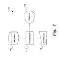
- FIG. 1 is a block diagram illustrating system components for implementing a method of performing structure-based Bayesian sparse signal reconstruction according to the present invention.
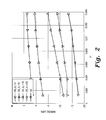
- FIG. 2 is a graph illustrating normalized mean-square error (NMSE) for varying cluster lengths compared against success probability in the method of performing structure-based Bayesian sparse signal reconstruction according to the present invention.
- NMSE normalized mean-square error
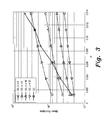
- FIG. 3 is a graph illustrating mean run time for varying cluster lengths compared against success probability in the method of performing structure-based Bayesian sparse signal reconstruction according to the present invention.
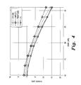
- FIG. 4 is a graph comparing normalized mean-square error (NMSE) against signal-to-noise ratio for the present method of performing structure-based Bayesian sparse signal reconstruction compared against the prior convex relaxation (CR) method, the orthogonal matching pursuit (OMP) method, and the fast Bayesian matching pursuit (FBMP) method for a sensing matrix which is a discrete Fourier transform (DFT) matrix and x
- NMSE normalized mean-square error
- CR convex relaxation
- OMP orthogonal matching pursuit
- FBMP fast Bayesian matching pursuit
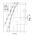
- FIG. 5 is a graph comparing normalized mean-square error (NMSE) against signal-to-noise ratio for the present method of performing structure-based Bayesian sparse signal reconstruction compared against the prior convex relaxation (CR) method, the orthogonal matching pursuit (OMP) method, and the fast Bayesian matching pursuit (FBMP) method for a sensing matrix which is a discrete Fourier transform (DFT) matrix and x
- NMSE normalized mean-square error
- CR convex relaxation
- OMP orthogonal matching pursuit
- FBMP fast Bayesian matching pursuit
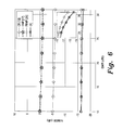
- FIG. 6 is a graph comparing normalized mean-square error (NMSE) against signal-to-noise ratio for the present method of performing structure-based Bayesian sparse signal reconstruction compared against the prior convex relaxation (CR) method, the orthogonal matching pursuit (OMP) method, and the fast Bayesian matching pursuit (FBMP) method for a sensing matrix which is a Toeplitz matrix and x
- NMSE normalized mean-square error
- CR convex relaxation
- OMP orthogonal matching pursuit
- FBMP fast Bayesian matching pursuit
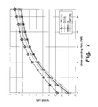
- FIG. 7 is a graph comparing normalized mean-square error (NMSE) against under-sampling ratio for the present method of performing structure-based Bayesian sparse signal reconstruction compared against the prior convex relaxation (CR) method, the orthogonal matching pursuit (OMP) method, and the fast Bayesian matching pursuit (FBMP) method for a sensing matrix which is a discrete Fourier transform (DFT) matrix and x
- NMSE normalized mean-square error
- CR convex relaxation
- OMP orthogonal matching pursuit
- FBMP fast Bayesian matching pursuit
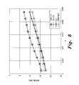
- FIG. 8 is a graph comparing normalized mean-square error (NMSE) against success probability for the present method of performing structure-based Bayesian sparse signal reconstruction compared against the prior convex relaxation (CR) method, the orthogonal matching pursuit (OMP) method, and the fast Bayesian matching pursuit (FBMP) method for a sensing matrix which is a discrete Fourier transform (DFT) matrix and x
- NMSE normalized mean-square error
- CR convex relaxation
- OMP orthogonal matching pursuit
- FBMP fast Bayesian matching pursuit
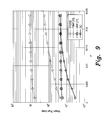
- FIG. 9 is a graph comparing mean run time against success probability for the present method of performing structure-based Bayesian sparse signal reconstruction compared against the prior convex relaxation (CR) method, the orthogonal matching pursuit (OMP) method, and the fast Bayesian matching pursuit (FBMP) method for a sensing matrix which is a discrete Fourier transform (DFT) matrix and x
- CR convex relaxation
- OMP orthogonal matching pursuit
- FBMP fast Bayesian matching pursuit
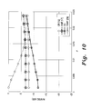
- FIG. 10 is a graph comparing normalized mean-square error (NMSE) against success probability for the present method of performing structure-based Bayesian sparse signal reconstruction compared against the prior convex relaxation (CR) method, the orthogonal matching pursuit (OMP) method, and the fast Bayesian matching pursuit (FBMP) method for a sensing matrix which is a discrete Fourier transform (DFT) matrix and x
- NMSE normalized mean-square error
- CR convex relaxation
- OMP orthogonal matching pursuit
- FBMP fast Bayesian matching pursuit
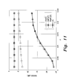
- FIG. 11 is a graph comparing normalized mean-square error (NMSE) against success probability for the present method of performing structure-based Bayesian sparse signal reconstruction compared against the prior convex relaxation (CR) method, the orthogonal matching pursuit (OMP) method, and the fast Bayesian matching pursuit (FBMP) method for a sensing matrix which is a Toeplitz matrix and x
- NMSE normalized mean-square error
- CR convex relaxation
- OMP orthogonal matching pursuit
- FBMP fast Bayesian matching pursuit
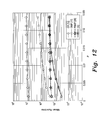
- FIG. 12 is a graph comparing mean run time against success probability for the present method of performing structure-based Bayesian sparse signal reconstruction compared against the prior convex relaxation (CR) method, the orthogonal matching pursuit (OMP) method, and the fast Bayesian matching pursuit (FBMP) method for a sensing matrix which is a Toeplitz matrix and x
- CR convex relaxation
- OMP orthogonal matching pursuit
- FBMP fast Bayesian matching pursuit
- x ⁇ C N is a P-sparse signal (i.e., a signal that consists of P non-zero coefficients in an N-dimensional space with P ⁇ N) in some domain
- the first step in the method is correlation of the observation vector y with the columns of the sensing matrix ⁇ . By retaining correlations that exceed a certain threshold, we can then determine the dominant positions/regions where the support of the sparse vector x is located. The performance of the orthogonal clustering method is dependent on this initial correlation-based estimate or “guess”. This step creates a vector of N correlations.
- the indices with a correlation greater than the threshold ⁇ are then obtained. Since n is complex Gaussian, the value of ⁇ can be easily evaluated such that p(
- each cluster is processed independently, and in each cluster, the likelihoods for supports of size
- 1,
- 2, . . . ,
- P c are calculated for each cluster, where P c denotes the maximum possible support size in a cluster.
- 1,
- 2, . . . ,
- Each cluster is processed independently by capitalizing on the semi-orthogonality between the clusters.
- the expected value of the sparse vector x given y and the most probable support for each size can also be evaluated using either equation (6) or equation (8), depending on the a priori statistical information.
- the MMSE (or MAP) estimates of x can be evaluated, as described above with respect to equation (31). It should be noted that these estimates are approximate, as they are evaluated using only the dominant supports instead of using all supports.
- x MMSE [ ⁇ Z 1 ⁇ S 1 ⁇ p ⁇ ( Z 1
- Z 1 . . . Z C are a set of dummy variables each ranging through a respective likelihood of support
- y, Z C ] are a set of expected values of the sparse vector x
- y) are a set of probable support sizes of the respective semi-orthogonal clusters.
- the first makes use of the orthogonality of the clusters. As will be described below, similarity of clusters and order within a cluster may also be taken advantage of.
- calculating the likelihood can be performed in a “divide-and-conquer” manner by calculating the likelihood for each cluster independently. This is a direct consequence of the semi-orthogonal structure of the columns of the sensing matrix. Further, due to the rich structure of the sensing matrix, the clusters formed are quite similar. Below, the structure present in discrete Fourier transform (DFT) and Toeplitz sensing matrices are used to show that the likelihood and expectation expressions in each cluster (for both the Gaussian and non-Gaussian cases) are strongly related, allowing many calculations across clusters to be shared.
- DFT discrete Fourier transform
- Toeplitz sensing matrices Toeplitz sensing matrices are used to show that the likelihood and expectation expressions in each cluster (for both the Gaussian and non-Gaussian cases) are strongly related, allowing many calculations across clusters to be shared.
- ⁇ 1 , ⁇ 2 , . . . , ⁇ L denote the sensing columns associated with the first cluster. Then, it can be seen that the corresponding columns for the i th cluster of equal length that are ⁇ i columns away are ⁇ 1 ⁇ ⁇ ⁇ i , ⁇ 2 ⁇ ⁇ i , . . . , ⁇ L ⁇ ⁇ 66 i , where ⁇ ⁇ i is some constant vector that depends on the sensing columns.
- equations (32) and (34) have the same sensing matrix and the same noise statistics (n is a white circularly symmetric Gaussian and, thus, is invariant to multiplication by ⁇ * ⁇ i ).
- y is modulated by the vector ⁇ * ⁇ i in moving from the first to the i th cluster. This allows us to write: p ( Z i
- y ) p ( Z 1
- y, Z i ] [x
- the ⁇ S i s are simply shifted versions of each other.
- ⁇ S ⁇ ′ ⁇ S + ⁇ x 2 ⁇ n 2 ⁇ ⁇ i ⁇ ⁇ i H or, by the matrix inversion lemma:
- the likelihood for the support of size S′ can be written as (using equations (44) and (45)):
- y] can be calculated in an order-recursive manner as follows:
- ⁇ S ′ [ ⁇ S + 1 ⁇ i ⁇ ⁇ i ⁇ ⁇ i H - 1 ⁇ i ⁇ ⁇ i - 1 ⁇ i ⁇ ⁇ i H 1 ⁇ i ] ( 48 )
- L S′ the projected norm
- calculations may be performed by any suitable computer system, such as that diagrammatically shown in the FIG. 1 .
- Data is entered into system 100 via any suitable type of user interface 116 , and may be stored in memory 112 , which may be any suitable type of computer readable and programmable memory and is preferably a non-transitory, computer readable storage medium.
- processor 114 which may be any suitable type of computer processor and may be displayed to the user on display 118 , which may be any suitable type of computer display.
- Processor 114 may be associated with, or incorporated into, any suitable type of computing device, for example, a personal computer or a programmable logic controller.
- the display 118 , the processor 114 , the memory 112 and any associated computer readable recording media are in communication with one another by any suitable type of data bus, as is well known in the art.
- Examples of computer-readable recording media include non-transitory storage media, a magnetic recording apparatus, an optical disk, a magneto-optical disk, and/or a semiconductor memory (for example, RAM, ROM, etc.).
- Examples of magnetic recording apparatus that may be used in addition to memory 112 , or in place of memory 112 , include a hard disk device (HDD), a flexible disk (FD), and a magnetic tape (MT).
- Examples of the optical disk include a DVD (Digital Versatile Disc), a DVD-RAM, a CD-ROM (Compact Disc-Read Only Memory), and a CD-R (Recordable)/RW.
- non-transitory computer-readable storage media include all computer-readable media, with the sole exception being a transitory, propagating signal.
- FIG. 2 compares the normalized mean-square error (NMSE) of the present method as the cluster length L is varied.
- NMSE normalized mean-square error
- the DFT matrix is used as the sensing matrix with x
- FIG. 3 shows that the smaller the length of clusters, the faster the algorithm. It should be noted that for larger values of L (e.g., L>32), it might not be possible to form the required number of non-overlapping clusters. To overcome this problem, the performance of OC implemented with variable length clusters is shown in FIG. 2 . In this case, the overlapping clusters are joined together to form larger clusters. It can be seen in FIG. 2 that the performance of OC with variable-length clusters is better than the case when it is implemented with fixed-length clusters. Moreover, this performance is achieved with a reasonable run-time, as shown in FIG. 3 .
- L e.g. 32
- FIG. 4 compares the performance of the algorithms for the case where the sensing matrix is a DFT matrix and x
- the number of greedy branches to explore (D) is set to 10. It should be noted that OC outperforms all other algorithms at low SNR, while FBMP performs quite close to it at SNR ⁇ 25 dB.
- S is unknown is shown in FIG. 5 .
- the entries of x G are drawn from a uniform distribution.
- FIG. 6 compares the performance of the algorithms for the case where the sensing matrix is Toeplitz. To do so, a Toeplitz matrix was first generated from a column having 20 non-zero consecutive samples drawn from a Gaussian distribution. The sensing matrix was then extracted by uniformly sub-sampling this full matrix at a rate less than the duration of the signal. It should be noted that the performance of OC and FBMP are almost the same at low SNR, but OC outperforms FBMP in the high SNR region. OMP and CR do not perform well in this case, as the sensing matrix does not exhibit the requisite incoherence conditions (in this case, ⁇ ( ⁇ ) ⁇ 0.9) on which much of the CS theory is based.
- FIG. 7 shows the performance of the algorithms (for the case where the sensing matrix is DFT and x
- the present method and FBMP perform quite close to each other with the present method performing slightly better at high (N/M) ratios.
- FIG. 8 compares the performance of the algorithms when the sparsity rate p is varied (for the case where the sensing matrix is DFT and x
- FIG. 9 compares the mean run-time of all of the algorithms. It can be seen that OC is faster than all other algorithms. As sparsity rate increases, the length of the clusters increases, and thus the complexity of OC.
- FIG. 10 shows that OC performs quite well at the low sparsity rate in the case where the sensing matrix is DFT and x
Landscapes
- Engineering & Computer Science (AREA)
- Artificial Intelligence (AREA)
- Computer Networks & Wireless Communication (AREA)
- Signal Processing (AREA)
- Image Analysis (AREA)
Abstract
Description
y=Ψx+n, (1)
where Ψ is an M×N measurement/sensing matrix that is assumed to be incoherent with the domain in which x is sparse, and n is complex additive white Gaussian noise, CN(0, σn 2Im). As M<<N, this is an ill-posed problem as there is an infinite number of solutions for x satisfying equation (1). If it is known a priori that x is sparse, the theoretical way to reconstruct the signal is to solve an l0-norm minimization problem using only M=2P measurements when the signal and measurements are free of noise:
where
For ll-norm minimization to reconstruct the sparse signal accurately, the sensing matrix Ψ should be sufficiently incoherent. In other words, the coherence, defined as μ(Ψ)
y=Ψ S x S +n. (4)
where the sum is over all the possible support sets S of x. The likelihood and expectation involved in equation (5) are evaluated below.
where
p(S)=p |S|(1−p)N−|S|. (10)
up to an irrelevant constant multiplicative factor, (1/πM), where ∥b∥A 2
{circumflex over (x)} MAP =
| TABLE 1 |
| Applications of Structured Sensing Matrices |
| Matrix Ψ | Application |
| Partial DFT | OFDM applications including peak-to-average power |
| ratio reduction, narrow-band interference cancelation | |
| and impulsive noise estimation and mitigation in DSL | |
| Toeplitz | Channel estimation, UWB and DOA estimation |
| Hankel | Wide-band spectrum sensing |
| DCT | Image compression |
| Structured Binary | Multi-user detection and contention resolution and |
| feedback reduction | |
which is a function of the difference, (k−k′) mod N. It thus suffices to consider the correlation of one column with the remaining ones. It should be noted that the matrix Ψ exhibits other structural properties (e.g., the fact that it is a Vandermonde matrix), which helps to reduce the complexity of MMSE estimation.
where the size of Θ depends on the sub-sampling ratio. Here, Ψk HΨk′=0 for |k−k′|>L, and thus the columns of Ψ can easily be grouped into truly orthogonal clusters. It should be noted that the individual columns of Θ are related to each other by a shift property.
where the equality in equation (18) is true up to some constant factor. To evaluate p(y|Z), we distinguish between the Gaussian and non-Gaussian cases. For brevity, focus is given to the Gaussian case and then these results are extrapolated to the non-Gaussian case. We know that
where
As ΨZ
Thus, we can write:
where
Using a similar procedure, we can decompose det (ΣZ) as:
where in going from equation (24) to equation (25), we used the fact that ΨZ
p(Z|y)≃πi=1 C p(Z i |y), (29)
which applies equally to the Gaussian and non-Gaussian cases.
where the last line follows from the fact that ΣZ
wherein Z1 . . . ZC are a set of dummy variables each ranging through a respective likelihood of support,
where Z1 . . . ZC are a set of dummy variables each ranging through a respective likelihood of support,
y=Ψ Z
y=Ψ Z
Using Hadamard multiplication by ψ*Δ
y⊙ψ* Δ
p(Z i |y)=p(Z 1 |y⊙ψ* Δ
and
which is valid for both the Gaussian and non-Gaussian cases. In other words, if Zi is obtained from Z1 by a constant shift, then any y-independent calculations remain the same while any calculations involving y are obtained by modulating y by the vector ψ*Δ
and, in the non-Gaussian case, it is given by:
and in the non-Gaussian case, we have:
for a set Z1 of columns of the first cluster. Then, an identical set of columns Zi are chosen in the ith cluster. From this:
where wi is a rectangular window corresponding to the location of the non-zero rows of ΨS
with
ΨS′ΨS′ H, it should be noted that
or, by the matrix inversion lemma:
Thus, using equation (41), we obtain:
The determinant of ΣS′ can be evaluated as follows:
Thus, the likelihood for the support of size S′ can be written as (using equations (44) and (45)):
The approach relies on calculating the inverse AS′
where
with the elements of ηi
Similarly, it can be seen that:
| TABLE 2 |
| Cluster-independent and Cluster-wise Evaluations in the Recursive |
| Procedure for Complexity Reduction Within a Cluster |
| Cluster Independent Evaluations | Cluster-wise Evaluations | |
| x|S is | Evaluate ωi and ξi using (42) | Evaluate ∥ ωi Hy ∥2 |
| Gaussian | and (43) | Update LS using (46) |
| Update ΣS −1 using (41) | Update |
|
| Update det (ΣS) using (45) | ||
| x|S is | Initialize: Calculate ψi H ψj ∀ i, j | Initialize: Evaluate yH ψi ∀ i |
| unknown | Evaluate ωi using (49) | Update LS using (51) |
| Update ΣS using (48) and (50) | Update |
|
and SNR=30 dB (unless stated otherwise). Cases where the sensing matrix is a DFT or a Toeplitz matrix were both simulated. In the Figures, the present orthogonal clustering-based method is represented as “OC”.
where x represents the estimated sparse signal for realization r, and R is the total number of runs. For this case, the DFT matrix is used as the sensing matrix with x|S being Gaussian. It should be noted that while implementing the present method with fixed-length clusters, overlapping of clusters is not allowed to maintain orthogonality. This results in an increase in the probability of missing the correct support if two supports are close to each other. Thus, the smaller the cluster, the greater the probability of missing the correct supports. This can be clearly seen in
Claims (10)
Priority Applications (1)
| Application Number | Priority Date | Filing Date | Title |
|---|---|---|---|
| US13/915,513 US8861655B1 (en) | 2013-06-11 | 2013-06-11 | Method of performing structure-based bayesian sparse signal reconstruction |
Applications Claiming Priority (1)
| Application Number | Priority Date | Filing Date | Title |
|---|---|---|---|
| US13/915,513 US8861655B1 (en) | 2013-06-11 | 2013-06-11 | Method of performing structure-based bayesian sparse signal reconstruction |
Publications (1)
| Publication Number | Publication Date |
|---|---|
| US8861655B1 true US8861655B1 (en) | 2014-10-14 |
Family
ID=51661184
Family Applications (1)
| Application Number | Title | Priority Date | Filing Date |
|---|---|---|---|
| US13/915,513 Expired - Fee Related US8861655B1 (en) | 2013-06-11 | 2013-06-11 | Method of performing structure-based bayesian sparse signal reconstruction |
Country Status (1)
| Country | Link |
|---|---|
| US (1) | US8861655B1 (en) |
Cited By (17)
| Publication number | Priority date | Publication date | Assignee | Title |
|---|---|---|---|---|
| US20150023608A1 (en) * | 2004-08-09 | 2015-01-22 | David Leigh Donoho | Method and apparatus for compressed sensing |
| CN107395210A (en) * | 2017-08-16 | 2017-11-24 | 姚静波 | Adaptive sparse based on sparse base error represents compression reconfiguration method and system |
| US10057383B2 (en) | 2015-01-21 | 2018-08-21 | Microsoft Technology Licensing, Llc | Sparsity estimation for data transmission |
| CN109190693A (en) * | 2018-08-27 | 2019-01-11 | 西安电子科技大学 | Variant target high Resolution Range Profile Identification method based on block management loading |
| CN109541549A (en) * | 2018-10-09 | 2019-03-29 | 广东工业大学 | The interrupted sampling repeater jammer suppressing method handled based on EMD and sparse signal |
| US10270624B2 (en) * | 2015-10-13 | 2019-04-23 | Samsung Electronics Co., Ltd. | Channel estimation method and apparatus for use in wireless communication system |
| CN110380994A (en) * | 2019-05-13 | 2019-10-25 | 上海海事大学 | Quick Bayesian matching tracks marine condition of sparse channel estimation method |
| CN110636017A (en) * | 2019-08-19 | 2019-12-31 | 江苏大学 | Downlink channel estimation method of large-scale MIMO system based on variational Bayesian inference |
| CN111555994A (en) * | 2020-05-22 | 2020-08-18 | 西北工业大学 | Cluster sparse channel estimation method based on maximum skip rule algorithm |
| CN111812644A (en) * | 2020-08-29 | 2020-10-23 | 西安电子科技大学 | MIMO radar imaging method based on sparse estimation |
| CN112272068A (en) * | 2020-10-23 | 2021-01-26 | 中国人民解放军空军工程大学 | Diversified interference estimation and suppression method based on multitask compressed sensing |
| CN112305495A (en) * | 2020-10-22 | 2021-02-02 | 南昌工程学院 | Method for reconstructing co-prime array covariance matrix based on atomic norm minimum |
| CN113346932A (en) * | 2021-05-19 | 2021-09-03 | 重庆邮电大学 | FSK signal diversity receiving method based on Bayesian data fusion |
| CN113556131A (en) * | 2021-07-21 | 2021-10-26 | 中国人民解放军国防科技大学 | Complex domain multitask Bayes compressed sensing method |
| CN113608192A (en) * | 2021-08-09 | 2021-11-05 | 广东工业大学 | Ground penetrating radar far field positioning method and device and computer readable storage medium |
| CN114584433A (en) * | 2022-02-24 | 2022-06-03 | 哈尔滨工程大学 | Method for detecting synchronous signal in multi-path channel under impulse noise environment |
| CN116567098A (en) * | 2023-07-10 | 2023-08-08 | 广东工业大学 | Signal reconstruction method and system with consistent mixed generalized expectations |
Citations (12)
| Publication number | Priority date | Publication date | Assignee | Title |
|---|---|---|---|---|
| US5539704A (en) | 1995-06-23 | 1996-07-23 | Western Atlas International, Inc. | Bayesian sequential Gaussian simulation of lithology with non-linear data |
| US20070206880A1 (en) | 2005-12-01 | 2007-09-06 | Siemens Corporate Research, Inc. | Coupled Bayesian Framework For Dual Energy Image Registration |
| US7269241B2 (en) | 2002-08-28 | 2007-09-11 | Ge Healthcare Finland Oy | Method and arrangement for medical X-ray imaging and reconstruction from sparse data |
| US7378660B2 (en) | 2005-09-30 | 2008-05-27 | Cardiovascular Imaging Technologies L.L.C. | Computer program, method, and system for hybrid CT attenuation correction |
| US20080129560A1 (en) * | 2005-05-10 | 2008-06-05 | Baraniuk Richard G | Method and Apparatus for Distributed Compressed Sensing |
| US20100246920A1 (en) * | 2009-03-31 | 2010-09-30 | Iowa State University Research Foundation, Inc. | Recursive sparse reconstruction |
| US7809155B2 (en) | 2004-06-30 | 2010-10-05 | Intel Corporation | Computing a higher resolution image from multiple lower resolution images using model-base, robust Bayesian estimation |
| WO2012037067A1 (en) | 2010-09-14 | 2012-03-22 | Massachusetts Institute Of Technology | Multi-contrast image reconstruction with joint bayesian compressed sensing |
| US8204715B1 (en) | 2010-03-25 | 2012-06-19 | The United States Of America As Represented By The Secretary Of The Navy | System and method for determining joint moment and track estimation performance bounds from sparse configurations of total-field magnetometers |
| US20120224498A1 (en) | 2011-03-04 | 2012-09-06 | Qualcomm Incorporated | Bayesian platform for channel estimation |
| US8274054B2 (en) | 2008-10-28 | 2012-09-25 | The Board Of Trustees Of The Leland Standford Junior University | Method and apparatus for imaging using robust bayesian sequence reconstruction |
| US20120249353A1 (en) * | 2011-02-25 | 2012-10-04 | California Institute Of Technology | Systems and methods for acquiring and decoding signals using compressed sensing |
-
2013
- 2013-06-11 US US13/915,513 patent/US8861655B1/en not_active Expired - Fee Related
Patent Citations (13)
| Publication number | Priority date | Publication date | Assignee | Title |
|---|---|---|---|---|
| US5539704A (en) | 1995-06-23 | 1996-07-23 | Western Atlas International, Inc. | Bayesian sequential Gaussian simulation of lithology with non-linear data |
| US7269241B2 (en) | 2002-08-28 | 2007-09-11 | Ge Healthcare Finland Oy | Method and arrangement for medical X-ray imaging and reconstruction from sparse data |
| US7809155B2 (en) | 2004-06-30 | 2010-10-05 | Intel Corporation | Computing a higher resolution image from multiple lower resolution images using model-base, robust Bayesian estimation |
| US20080129560A1 (en) * | 2005-05-10 | 2008-06-05 | Baraniuk Richard G | Method and Apparatus for Distributed Compressed Sensing |
| US7378660B2 (en) | 2005-09-30 | 2008-05-27 | Cardiovascular Imaging Technologies L.L.C. | Computer program, method, and system for hybrid CT attenuation correction |
| US20070206880A1 (en) | 2005-12-01 | 2007-09-06 | Siemens Corporate Research, Inc. | Coupled Bayesian Framework For Dual Energy Image Registration |
| US8274054B2 (en) | 2008-10-28 | 2012-09-25 | The Board Of Trustees Of The Leland Standford Junior University | Method and apparatus for imaging using robust bayesian sequence reconstruction |
| US20100246920A1 (en) * | 2009-03-31 | 2010-09-30 | Iowa State University Research Foundation, Inc. | Recursive sparse reconstruction |
| US8204715B1 (en) | 2010-03-25 | 2012-06-19 | The United States Of America As Represented By The Secretary Of The Navy | System and method for determining joint moment and track estimation performance bounds from sparse configurations of total-field magnetometers |
| WO2012037067A1 (en) | 2010-09-14 | 2012-03-22 | Massachusetts Institute Of Technology | Multi-contrast image reconstruction with joint bayesian compressed sensing |
| US20120249353A1 (en) * | 2011-02-25 | 2012-10-04 | California Institute Of Technology | Systems and methods for acquiring and decoding signals using compressed sensing |
| US20120224498A1 (en) | 2011-03-04 | 2012-09-06 | Qualcomm Incorporated | Bayesian platform for channel estimation |
| WO2012122037A1 (en) | 2011-03-04 | 2012-09-13 | Qualcomm Incorporated | Bayesian platform for channel estimation |
Non-Patent Citations (3)
| Title |
|---|
| A.A. Quadeer, S.F. Ahmed and T.Y. Al-Naffouri, "Structure based Bayesian sparse reconstruction using non-Gaussian prior", Communication, Control, and Computing (Allerton), 2011 49th Annual Allerton Conference on, Sep. 28-30, 2011, pp. 277-283. |
| Mudassir Masood and Tareq Al-Naffouri, "A Fast Non-Gaussian Bayesian Matching Pursuit Method for Sparse Reconstruction", published on arXiv.org on Jun. 19, 2012. |
| X. Tan and J. Li, "Computationally Efficient Sparse Bayesian Learning via Belief Propagation", Signal Processing, IEEE Transactions on, vol. 58, Issue 4, pp. 2010-2021, Apr. 2010. |
Cited By (29)
| Publication number | Priority date | Publication date | Assignee | Title |
|---|---|---|---|---|
| US20150023608A1 (en) * | 2004-08-09 | 2015-01-22 | David Leigh Donoho | Method and apparatus for compressed sensing |
| US9626560B2 (en) * | 2004-08-09 | 2017-04-18 | The Board Of Trustees Of The Leland Stanford Junior University | Method and apparatus for compressed sensing |
| US10057383B2 (en) | 2015-01-21 | 2018-08-21 | Microsoft Technology Licensing, Llc | Sparsity estimation for data transmission |
| US10270624B2 (en) * | 2015-10-13 | 2019-04-23 | Samsung Electronics Co., Ltd. | Channel estimation method and apparatus for use in wireless communication system |
| CN107395210A (en) * | 2017-08-16 | 2017-11-24 | 姚静波 | Adaptive sparse based on sparse base error represents compression reconfiguration method and system |
| CN109190693A (en) * | 2018-08-27 | 2019-01-11 | 西安电子科技大学 | Variant target high Resolution Range Profile Identification method based on block management loading |
| CN109190693B (en) * | 2018-08-27 | 2022-03-22 | 西安电子科技大学 | Variant target high-resolution range profile recognition method based on block sparse Bayesian learning |
| CN109541549A (en) * | 2018-10-09 | 2019-03-29 | 广东工业大学 | The interrupted sampling repeater jammer suppressing method handled based on EMD and sparse signal |
| CN109541549B (en) * | 2018-10-09 | 2023-03-07 | 广东工业大学 | Intermittent sampling forwarding interference suppression method based on EMD and sparse signal processing |
| CN110380994A (en) * | 2019-05-13 | 2019-10-25 | 上海海事大学 | Quick Bayesian matching tracks marine condition of sparse channel estimation method |
| CN110380994B (en) * | 2019-05-13 | 2021-09-07 | 上海海事大学 | Fast Bayesian matching pursuit marine sparse channel estimation method |
| CN110636017A (en) * | 2019-08-19 | 2019-12-31 | 江苏大学 | Downlink channel estimation method of large-scale MIMO system based on variational Bayesian inference |
| CN110636017B (en) * | 2019-08-19 | 2022-02-15 | 江苏大学 | Downlink channel estimation method of large-scale MIMO system based on variational Bayesian inference |
| CN111555994B (en) * | 2020-05-22 | 2021-04-02 | 西北工业大学 | Cluster sparse channel estimation method based on maximum skip rule algorithm |
| CN111555994A (en) * | 2020-05-22 | 2020-08-18 | 西北工业大学 | Cluster sparse channel estimation method based on maximum skip rule algorithm |
| CN111812644A (en) * | 2020-08-29 | 2020-10-23 | 西安电子科技大学 | MIMO radar imaging method based on sparse estimation |
| CN112305495A (en) * | 2020-10-22 | 2021-02-02 | 南昌工程学院 | Method for reconstructing co-prime array covariance matrix based on atomic norm minimum |
| CN112305495B (en) * | 2020-10-22 | 2023-10-13 | 南昌工程学院 | Method for reconstructing covariance matrix of cross matrix based on atomic norm minimum |
| CN112272068A (en) * | 2020-10-23 | 2021-01-26 | 中国人民解放军空军工程大学 | Diversified interference estimation and suppression method based on multitask compressed sensing |
| CN113346932A (en) * | 2021-05-19 | 2021-09-03 | 重庆邮电大学 | FSK signal diversity receiving method based on Bayesian data fusion |
| CN113346932B (en) * | 2021-05-19 | 2022-06-21 | 重庆邮电大学 | FSK signal diversity receiving method based on Bayesian data fusion |
| CN113556131B (en) * | 2021-07-21 | 2022-05-03 | 中国人民解放军国防科技大学 | Complex domain multitask Bayes compressed sensing method |
| CN113556131A (en) * | 2021-07-21 | 2021-10-26 | 中国人民解放军国防科技大学 | Complex domain multitask Bayes compressed sensing method |
| CN113608192B (en) * | 2021-08-09 | 2022-02-18 | 广东工业大学 | Ground penetrating radar far field positioning method and device and computer readable storage medium |
| CN113608192A (en) * | 2021-08-09 | 2021-11-05 | 广东工业大学 | Ground penetrating radar far field positioning method and device and computer readable storage medium |
| CN114584433A (en) * | 2022-02-24 | 2022-06-03 | 哈尔滨工程大学 | Method for detecting synchronous signal in multi-path channel under impulse noise environment |
| CN114584433B (en) * | 2022-02-24 | 2024-05-28 | 哈尔滨工程大学 | Synchronous signal detection method in multi-path channel under impulse noise environment |
| CN116567098A (en) * | 2023-07-10 | 2023-08-08 | 广东工业大学 | Signal reconstruction method and system with consistent mixed generalized expectations |
| CN116567098B (en) * | 2023-07-10 | 2023-09-15 | 广东工业大学 | Signal reconstruction method and system with consistent mixed generalized expectations |
Similar Documents
| Publication | Publication Date | Title |
|---|---|---|
| US8861655B1 (en) | Method of performing structure-based bayesian sparse signal reconstruction | |
| Pal et al. | Pushing the limits of sparse support recovery using correlation information | |
| Guo et al. | A single-letter characterization of optimal noisy compressed sensing | |
| US9806912B2 (en) | Methods and devices for channel estimation and OFDM receiver | |
| US9804999B2 (en) | Signal/noise separation using FrFT rotational parameter obtained in relation to Wigner Distribution | |
| US8139656B2 (en) | Method and system for linear processing of an input using Gaussian belief propagation | |
| US20090003483A1 (en) | Detector and Method for Estimating Data Probability in a Multi-Channel Receiver | |
| US9008211B2 (en) | Receiving device, receiving method, and receiving program | |
| Meenakshi | A survey of compressive sensing based greedy pursuit reconstruction algorithms | |
| Quadeer et al. | Structure-based Bayesian sparse reconstruction | |
| Barbu et al. | OFDM receiver for fast time-varying channels using block-sparse Bayesian learning | |
| Ji et al. | On gradient descent algorithm for generalized phase retrieval problem | |
| Parker | Approximate message passing algorithms for generalized bilinear inference | |
| Asif et al. | Random channel coding and blind deconvolution | |
| Wen et al. | Analysis of compressed sensing with spatially-coupled orthogonal matrices | |
| Quadeer et al. | Structure based Bayesian sparse reconstruction using non-Gaussian prior | |
| Thomas et al. | Recovery from compressed measurements using sparsity independent regularized pursuit | |
| de Paiva et al. | Sparsity analysis using a mixed approach with greedy and LS algorithms on channel estimation | |
| Ambat et al. | On selection of search space dimension in compressive sampling matching pursuit | |
| US9318232B2 (en) | Matrix spectral factorization for data compression, filtering, wireless communications, and radar systems | |
| Chatterjee et al. | Projection-based atom selection in orthogonal matching pursuit for compressive sensing | |
| Huang et al. | Sparse signal recovery using structured total maximum likelihood | |
| RU2658335C1 (en) | Method of joint evaluation of communication channel and soft demodulation for cofdm signals and device for its implementation | |
| Masood et al. | A fast non-gaussian bayesian matching pursuit method for sparse reconstruction | |
| Joseph et al. | Sparsity-aware Bayesian inference and its applications |
Legal Events
| Date | Code | Title | Description |
|---|---|---|---|
| AS | Assignment |
Owner name: KING FAHD UNIVERSITY OF PETROLEUM AND MINERALS, SA Free format text: ASSIGNMENT OF ASSIGNORS INTEREST;ASSIGNORS:AL-NAFFOURI, TAREQ Y., DR.;QUADEER, AHMED ABDUL, MR.;SIGNING DATES FROM 20130603 TO 20130604;REEL/FRAME:030590/0944 Owner name: KING ABDULAZIZ CITY FOR SCIENCE AND TECHNOLOGY, SA Free format text: ASSIGNMENT OF ASSIGNORS INTEREST;ASSIGNORS:AL-NAFFOURI, TAREQ Y., DR.;QUADEER, AHMED ABDUL, MR.;SIGNING DATES FROM 20130603 TO 20130604;REEL/FRAME:030590/0944 |
|
| STCF | Information on status: patent grant |
Free format text: PATENTED CASE |
|
| MAFP | Maintenance fee payment |
Free format text: PAYMENT OF MAINTENANCE FEE, 4TH YEAR, LARGE ENTITY (ORIGINAL EVENT CODE: M1551) Year of fee payment: 4 |
|
| FEPP | Fee payment procedure |
Free format text: MAINTENANCE FEE REMINDER MAILED (ORIGINAL EVENT CODE: REM.); ENTITY STATUS OF PATENT OWNER: LARGE ENTITY |
|
| LAPS | Lapse for failure to pay maintenance fees |
Free format text: PATENT EXPIRED FOR FAILURE TO PAY MAINTENANCE FEES (ORIGINAL EVENT CODE: EXP.); ENTITY STATUS OF PATENT OWNER: LARGE ENTITY |
|
| STCH | Information on status: patent discontinuation |
Free format text: PATENT EXPIRED DUE TO NONPAYMENT OF MAINTENANCE FEES UNDER 37 CFR 1.362 |
|
| FP | Lapsed due to failure to pay maintenance fee |
Effective date: 20221014 |