US8768874B2 - Predicting the outcome of a chaotic system using Lyapunov exponents - Google Patents
Predicting the outcome of a chaotic system using Lyapunov exponents Download PDFInfo
- Publication number
- US8768874B2 US8768874B2 US13/082,824 US201113082824A US8768874B2 US 8768874 B2 US8768874 B2 US 8768874B2 US 201113082824 A US201113082824 A US 201113082824A US 8768874 B2 US8768874 B2 US 8768874B2
- Authority
- US
- United States
- Prior art keywords
- chaotic system
- lyapunov exponent
- lyapunov
- trajectory
- chaotic
- Prior art date
- Legal status (The legal status is an assumption and is not a legal conclusion. Google has not performed a legal analysis and makes no representation as to the accuracy of the status listed.)
- Expired - Fee Related, expires
Links
Images
Classifications
-
- G—PHYSICS
- G06—COMPUTING; CALCULATING OR COUNTING
- G06N—COMPUTING ARRANGEMENTS BASED ON SPECIFIC COMPUTATIONAL MODELS
- G06N7/00—Computing arrangements based on specific mathematical models
- G06N7/08—Computing arrangements based on specific mathematical models using chaos models or non-linear system models
Definitions
- the invention relates to predicting the outcome of a chaotic system. More particularly, the invention relates to predicting outcome of chaotic systems using Lyapunov exponents.
- Chaotic non-linear systems are known. Examples of chaotic systems include, but are not limited to, the weather, the stock market and fluid flow. By its nature, it is difficult to calculate the outcome of a chaotic system. A slight change in initial conditions or an intervening event can result in a completely different outcome or trajectory. In a weather system, a slight change in the initial conditions of temperatures and pressures at various locations results in a completely different weather trajectory. As a result, a long range forecast may be difficult or impossible to make.
- One way that chaotic systems can be defined is by calculating a Lyapunov exponent, which is a measure of the rate of divergence of a trajectory with time.
- the present invention provides a system and method for predicting the outcome of a chaotic system.
- a prediction system includes means for varying the initial conditions of a chaotic system and means for calculating a plurality of possible trajectories for the chaotic system.
- the prediction system also includes means for calculating a Lyapunov exponent for each of the plurality of possible trajectories and means for selecting the trajectory with the smallest Lyapunov exponent as the most likely trajectory to occur.
- a method of predicting the likelihood of an outcome in a chaotic system is also provided.
- the method generally includes varying initial conditions of a mathematical model of a chaotic system and calculating multiple trajectories of the chaotic system model based on a number of uncertainty factors.
- the method includes calculating a Lyapunov exponent for each of the multiple trajectories and comparing the Lyapunov exponents from each of the multiple trajectories to determine the trajectory with the smallest Lyapunov exponent, whereby the trajectory with the smallest Lyapunov exponent is indicative of the likelihood of the outcome of the chaotic system.
- a computer program disclosed herein is stored on a computer readable medium for execution by a computer.
- the computer program includes logic elements that vary the initial conditions of a chaotic system and calculate a plurality of possible trajectories for the chaotic system.
- the computer program also includes logic configured to calculate a Lyapunov exponent for each of the plurality of possible trajectories to determine the trajectory with the smallest Lyapunov exponent and to select the trajectory with the smallest Lyapunov exponent to represent a prediction of an outcome of the chaotic system.
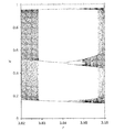
- FIG. 1 is a graph of a period-3 window of a logistic map.
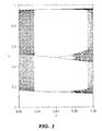
- FIG. 2 is a histogram of an iteration count for the logistic map of FIG. 1 .
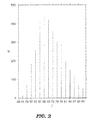
- FIG. 3 is a graph showing the convergence of the maximum Lyapunov exponent over time.
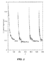
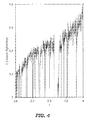
- FIG. 4 is a graph of a Lyapunov exponent for the logistic map of FIG. 1 .
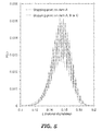
- FIG. 5 is a graph of a normalized distribution of local Lyapunov exponents for the logistic map of FIG. 1 .
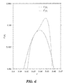
- FIG. 6 is a graph of two super cycles for the logistic map of FIG. 1 .
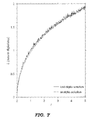
- FIG. 7 is a graph of the maximum Lyapunov exponent for a two-dimensional map and analytic curve.
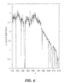
- FIG. 8 is a graph of the maximum Lyapunov exponent for the Lorenz equations averaged over nine exponents.
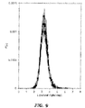
- FIG. 9 is a graph of a first normalized distribution of local Lyapunov exponents for the Lorenz system.
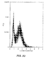
- FIG. 10 is a graph of a second normalized distribution of local Lyapunov exponents for the Lorenz system.
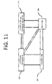
- FIG. 11 is a high level block diagram of a general purpose computer suitable for use in performing functions of the software described herein.
- Suggested chaotic systems may include, but are not limited, weather systems, fluid flow systems, traffic patterns, the stock market and other dynamic systems that are sensitive to initial conditions.
- An accurate prediction of the chaotic systems can be made using the systems and methods of the invention and can be calculated using less computational complexity than previously known systems.
- weather systems also referred to as weather maps
- the invention can accurately and quickly forecast or predict the weather patterns in various locations.
- fluid flow systems the invention can predict liquid flow through a conduit or around a structure, such as a dam, spillway, watercraft and so forth.
- Fluid flow systems may also include air flow systems, such as those which may be used to design an airplane or other aircraft.
- traffic systems the invention can be used to predict patterns of vehicular traffic on a road or network of roads.
- the invention can predict outcome of such chaotic systems by comparing single-precision calculations with double-precision calculations to determine the maximal Lyapunov exponent.
- the resulting maximal Lyapunov exponent is found in less than one-tenth of the computational time required by traditional methods.
- this algorithm can be applied to both maps, such as weather forecast maps, and systems of differential equations.
- This algorithm is easily coded because it is free of Jacobians, tangent vectors, Gramm-Schmidt procedures, overflow errors, and trial-and-error parameters.
- the algorithm is applicable to any numerical time evolution procedure and can be applied where no existing routine is available, e.g. recursion relations or to the successive terms of a series, as often exist in quantum mechanical calculations. It is shown herein that the maximum Lyapunov exponent can be experimentally measured by comparing two data runs of the chaotic system at different levels of precision.
- Lyapunov exponent plots and local Lyapunov exponent distributions are given for the logistic map and the Lorenz equations. Restricted error regions are discussed where the Lyapunov exponent is greater than zero, but the error magnitude is restricted to a fraction of the size of the available phase space.
- An empirical formula is also provided which can quickly calculate the r ⁇ point of a period p window.
- a trajectory having a large Lyapunov exponent, large rate of divergence, will be less likely to occur than one having a small Lyapunov exponent, small rate of divergence.
- the analysis of chaotic systems using the Lyapunov exponents can also be used to determine the most likely trajectory.
- the initial conditions of the system can be varied within their initial uncertainties to calculate several possible trajectories.
- the Lyapunov exponents from each of these trajectories are then be calculated.
- the trajectory having the smallest Lyapunov exponent is the most likely to occur.
- the time rate of loss of the number of digits, dn/dt can be determined by comparing single-precision and double-precision calculations of the system's trajectories to produce maximal Lyapunov exponents more quickly and easily than previous techniques.
- the invention can be applied, without alteration, to both maps, such as weather maps, and systems of differential equations, and can be applied to any time evolution system. For example it can be applied to recursion relations, the Gramm-Schmidt re-orthogonalization procedure and the like. It has been used to determine Lyapunov exponents in the chaotic behavior found in a first number of partial sums, e.g. the first 50 partial sums, of a series describing the electromagnetic scattering from a pair of overlapping spheres. This lost digits technique can be used to test for divergence between two calculations of differing precision, which describes the time evolution in quantum mechanical systems.
- the invention also provides a computer program that uses the source code of the non-linear system as a subroutine.
- the input to the computer program includes the initial conditions and the relative uncertainties of these conditions. For instance, in a weather program, the input includes the temperature and pressure at various locations and uncertainties associated with these input values.
- the main program would calculate various trajectories and Lyapunov exponents of these trajectories. It would then determine the smallest exponent and assign this as the most likely outcome.
- the system of the invention for calculating Lyapunov exponents using single precision and double precision values for predicting the outcome of chaotic systems can be implemented in software, hardware, or a combination thereof.
- the system is implemented in software as an executable computer program and is executed by a general purpose digital computer or other suitable digital processing device.
- the software may be stored in memory in any suitable format and may include one or more separate programs.
- the software includes an ordered listing of executable instructions for implementing logical functions.
- the software may be a computer program, source program, executable program, object code, script or any other entity that can include a set of instructions to be performed.
- the system of the invention for calculating Lyapunov exponents can be stored on any computer readable medium for use by or in connection with any computer related system or method.
- a computer readable medium is any electronic, magnetic, electromagnetic, optical, infrared or semiconductor system, apparatus, device, or propagation medium or other suitable physical device or means that can contain or store a computer program for use by or in connection with a computer related system or method.
- the system for calculating Lyapunov exponents may be configured using physical or electrical components, modules, and/or processing means for performing various functions.
- these functional components, modules and processing means are capable of varying the initial conditions of a chaotic system model and then calculating trajectories for the chaotic system.
- they are further capable of calculating a Lyapunov exponent for each trajectory and selecting a trajectory with the smallest Lyapunov exponent to determine the most likely predictable outcome of the chaotic system.
- Equation 4 can be rewritten by isolating f′ from Equation 6:
- Equations 5, 7 and 8 are also valid in any time evolution including recursion relations, or q-dimensional systems of differential equations, when the error ⁇ is replaced with
- the rate of change of valid digits dn/dt can be determined by continually comparing single-precision calculations with double-precision calculations of the system trajectory, in which X s (t) and X d (t) represent the system's trajectory at a single-precision level and a double-precision level, respectively.
- the single precision, lower precision may be defined by a variable using a first number of bits, e.g. 16 bits.
- the double-precision, higher precision may be defined by a variable using a second and higher number of bits, e.g. 32 bits.
- a quad precision including 64 bits may be used. Other precisions may be used in accordance with the capabilities of available processing equipment.
- n(t) most significant digits of X s (t) match the corresponding digits of X d (t).
- ⁇ ⁇ ( t ) ⁇ X s ⁇ ( t ) - X d ⁇ ( t ) X d ⁇ ( t ) ⁇ .
- , when the initial values are set so as to avoid a zero in the denominator: X s (0) X d (0)[1+2 ⁇ 10 ⁇ Ws ]. (13) Note that computers can more accurately represent numbers that are integral powers of two, and that they treat X s (0) as a binary number.
- Equation 5 is expressed as a natural exponential function, the base of the digits is natural, base e.
- ⁇ j ⁇ o b Lj .
- the natural base is used in order to compare the results with those of previous publications.
- the time evolution might be the successive iterations of a map, the successive time steps of a system of differential equations, the successive terms of a recursion relation, the successive partial sums of a series or any function of time, f(t), including quantum mechanical functions.
- X s (t) and X d (t) can also be two repeated runs of an experiment if enough significant digits are initially available.
- these systems could only be evaluated as time series, and hundreds or thousands of points were needed to compute the Lyapunov exponent.
- the present lost digits technique can be applied to as few as about 50 iterations.
- the lost digits algorithm is straightforward.
- the system is integrated or iterated until most of the digits of X s and X d disagree.
- the system is evolved until an error threshold ⁇ >0.01 X d (18) is reached.
- This arbitrary criterion can be referred to as the lost digits stopping point.
- Equations 17 and 18 represent the lost digits technique.
- An algorithm for calculating the Lyapunov exponents using this method and any currently existing computer code is discussed at the end of this section. The choice of 0.01 for this fractional error is arbitrary and may be replaced by any other suitable fraction.
- ⁇ is allowed to grow to involve the most significant digits, then the widths of the local exponent distributions become smaller, the width going to zero as W s ⁇ .
- Equation 6 the jth error is due to the product of the q local slopes and the previous error, i.e.,
- d X j ( i ) d X j - 1 ( i ) ⁇ i ⁇ ⁇ ⁇ g i / ⁇ X ( i ) ⁇ ⁇ d X j ( i ) ⁇ i ⁇ ⁇ ⁇ g i / ⁇ X ( i ) ⁇ ⁇ d X j - 1 ( i ) ( 26 ) where g f (t ⁇ 1).
- Equations 24 and 26 can be combined to calculate the maximal Lyapunov exponent
- this technique is computationally advantageous to previous techniques using Runge-Kutta algorithms, e.g. the Bennetin and Wolf algorithms.
- the present technique requires calculating two distinct trajectories using single- and double-precision, the previous techniques require one trajectory in double precision plus an associated system of q 2 dimensions stemming from the Jacobian of the system.
- the Runge-Kutta and Gramm-Schmidt procedures require a great deal of additional calculations.
- the error in these other techniques is not 10 ⁇ Ws , but set to unit magnitude.
- Equation 17 or 20 provides a procedure for the direct measurement of Lyapunov exponents.
- the system is run twice from identical initial conditions for a certain elapsed time and then the difference between the two runs is calculated throughout the elapsed time.
- the following considerations should be taken into account.
- the lost digits Lyapunov exponent is not due to a single iteration or integration time step, or an infinite number of them, but is instead due to a small number of time steps.
- the Lyapunov exponent can be calculated from the product of the 50 or so error magnifications that the trajectory encounters.
- the lost-digits technique as described herein determines an exponent after every ten-second trajectory segment. For this reason, the lost digit approach can be said to produce only regional exponents.
- the lost digits technique typically produces a global exponent only for the case W s ⁇ .
- FIG. 1 For reference, an example of a period-3 window of a logistic map is shown in FIG. 1 .
- X j+1 rX j (1 ⁇ X j ).
- the lost digits stopping point can never be reached when the iteration lands on this central band.
- the initial value X o usually is not located on any of the three bands.
- the iteration lands on the central band at the kth iteration.
- the lost digits stopping point is usually reached after the second successive error growth iteration out of the grow-grow-shrink pattern, so that the stopping point occurs only in integer multiples of three iterations That is, the elapsed time (the denominator in Equation 5) only contains the integers k+2+3j. This is shown in the histogram of iteration counts needed to reach the lost-digits stopping point ( FIG. 2 ).
- FIG. 3 shows the Lyapunov exponent calculated as a function of iteration count.
- the plot shows how the exponent asymptotically approaches a final value as the count increases.
- X s (t) X d (t) and repeat the process.
- the calculated error decreases when the iteration lands on the central band and increases when the iteration lands on the other two bands, and consequently the calculated Lyapunov exponent is smaller if the experiment is stopped when the iteration lands on the central band and is larger if the experiment is stopped on the other two bands.
- the amplitude of these oscillations dies down.
- This plot demonstrates that a meaningful exponent has not been computed until enough digits have been lost so that the exponent approximates its asymptotic value. This also means that the lost digits technique does not normally produce a single step local exponent. This result can also be reached if we consider the three bands in the case of Table 1. Since the error, Lyapunov exponent, grows on two bands and recedes on one band, the first iteration is usually unable to determine the value of the Lyapunov exponent or even the correct sign.
- FIG. 4 is a plot of the Lyapunov exponent for the logistic map. Each trajectory has its own exponent and the noise is produced by the natural variation of the local exponents. This plot is noisy but rapidly produced. If desired, the noise can be reduced by averaging. The averaging of exponents has been performed in three different ways:
- FIG. 5 A plot of the distributions of local exponents for the parameters of FIG. 2 is shown in FIG. 5 .
- the parameter values in FIG. 5 were chosen near the end of a periodic window where oscillations appear in the distribution (solid line). These oscillations are a result of the stopping point criterion never being satisfied on bands B or C.
- FIG. 5 also shows the distribution (dashed line) when the method of terminating the experiment is chosen. In this case, the map is in a restricted error region as defined below. Note that most Lyapunov distributions are smooth and do not contain these oscillations. Although the artifact is easily removed from the distribution, it is of interest because it indicates that the map is in an interesting or unusual region.
- the iterations X j are always known to within a maximum error equal to the width of the largest region.
- the Lyapunov exponent is positive for a particular range of r values, but at least one valid digit is retained in the computed trajectory, then we refer to that parameter region as a restricted error region.
- the trajectory is not 100% uncertain.
- a physical system is always limited to a finite phase space. These restricted error regions always occur near the ends of periodic windows where the system is returning to chaos. These regions are readily apparent in the bifurcation diagrams and Lyapunov exponent plots of published systems. They become smaller in higher period windows, which increases the number of digits that remain valid.
- the r ⁇ value for the period-3 window is r ⁇ ⁇ 3.84950. It can be found in this and numerous other calculations that r b ⁇ r ⁇ . This result is useful, since the r ⁇ value is much more difficult to determine than the equal slope condition.
- FIG. 7 shows the Lyapunov exponents using the lost-digits technique (solid line) and the analytic solution (dashed line) for the largest Lyapunov exponent for this map.
- the lost-digits technique is able to quickly reproduce the results of Equation 34.
- the lost digits Lyapunov exponents are computed by comparing 16 and 20 , for example, significant-digit solutions with a stopping point given by Equation 18.
- the lost digits exponent is averaged over 9 initial conditions using a constant Runge-Kutta step size of 0.02 and integrated for a maximum of 100,000 time steps, so that a tiny positive exponent could be found if it occurred. The results shown in FIG.
- the number of valid digits is a direct measure of the information that is known about a system. This fact can be used to provide several methods of determining Lyapunov exponents. Maximal Lyapunov exponents are determined by the time rate of change of the number of valid digits in the system's trajectory and can be computed by combining the stopping point given by Equation 18 with either of Equations 5, 17, 19, or 20. For a flow system, the stopping point can also be combined with Equation 23, 25, or 26. The Lyapunov exponent can be experimentally measured by comparing two separate runs of a system, and applying Equations 17 and 18. This method allows Lyapunov exponents to be calculated in less than one-tenth of the computational time required by traditional methods.
- the distribution of local Lyapunov exponents explains the noise seen in maximal Lyapunov exponent plots.
- a distribution of local exponents occurs because the error growth rate of any segment of a trajectory is due to the product of local slopes which are encountered by that segment.
- the variation in local exponents is simply a factor of the variation in local slopes.
- An oscillation in the distribution indicates that some interesting feature of the trajectory is causing certain integer counts to be absent from the lost-digits stopping time.
- the magnitude of the system's error is found to be specially restricted near the end of periodic windows, even though L>0 in these regions.
- FIG. 11 depicts a high level block diagram of a general purpose computer suitable for use in performing the functions described above as well as claimed below.
- the system 200 includes a processor element 202 (e.g., a CPU) for controlling the overall function of the system 200 .
- Processor 202 operates in accordance with stored computer program code, which is stored in memory 204 .
- Memory 204 represents any type of computer readable medium and may include, for example, RAM, ROM, optical disk, magnetic disk, or a combination of these media.
- the processor 202 executes the computer program code in memory 204 in order to control the functioning of the system 200 .
- Processor 202 is also connected to network interface 205 , which transmits and receives network data packets.
- various input/output devices 206 e.g., storage devices, including but not limited to, a tape drive, a floppy drive, a hard disk drive or compact disk drive, a receiver, a transmitter, a speaker, a display, a speech synthesizer, an output port, and a user input device (such as a keyboard, a keypad, a mouse and the like)).
- storage devices including but not limited to, a tape drive, a floppy drive, a hard disk drive or compact disk drive, a receiver, a transmitter, a speaker, a display, a speech synthesizer, an output port, and a user input device (such as a keyboard, a keypad, a mouse and the like)
- a user input device such as a keyboard, a keypad, a mouse and the like
Abstract
Description
X j =f j(X o) (1)
where Xo is the initial value. When a small error εn is found to grow exponentially, the system is said to be chaotic. The error in the jth iteration is found using the chain rule as
where Lyapunov exponent L is defined as
The ratio |εj/εo| gives the total error magnification and its log gives the number of digits needed to express the error growth. The number of lost digits is given by the number of digits in the error. From
εj+1 =f′εj (6)
This means the current error is magnified by the local slope to produce the next error, and the local error increases or decreases when the local slope is greater than one (or less than one). The Lyapunov exponent is the result of these error magnifications. A pictorial representation of this is shown in the cited Schuster reference on page 25. A range in the abscissa is magnified by the slope to produce a range in the function ƒ(x). It is stressed that the local Lyapunov exponent given by the accumulated error for any finite length trajectory segment is due to the products of local slopes that the segment encounters. This is the cause of the variation in the local exponents and produces the distributions discussed later. This also causes the noise seen in maximal Lyapunov exponent plots.
For numerical calculations this is more rapidly computed from
Also note that
In the past, the use of these equations has been restricted to one-dimensional maps. When used with the lost digits technique, they can be applied to q-dimensional systems, as discussed later.
Determining L(t) from the Rate of Change of Valid Digits
X s(t=0)=X d(t=0)=X 0. (10)
Initially, the Ws, most significant digits of Xd(t) agree with the corresponding digits of Xs(t), and the number of valid digits is n(t=0)=Ws. The two copies of the system are then independently integrated or iterated with respect to time. At any later time only the n(t) most significant digits of Xs(t) match the corresponding digits of Xd(t). For chaotic systems with exponential error growth, n(t) decreases linearly in time. Since Xd(t) is always known to a greater precision than Xs(t), the error in Xs(t) can be written as
ε(t)=|X s(t)−X d(t)|, (11)
and the fractional error is
The Lyapunov exponent can be calculated from
X s(0)=X d(0)[1+2·10−Ws]. (13)
Note that computers can more accurately represent numbers that are integral powers of two, and that they treat Xs(0) as a binary number.
The non-integral number of digits needed to write down the error is log (ε) so this numerator m(t) represents the number of decimal digits that have been lost
also represents the number of decimal digits lost). The Lyapunov exponent is then
L=−dn/dt≈−(n final −n initial)/t=m(t)/t, (15)
where t is the elapsed time in a continuous system or the number of iterations in a discrete map. The derivative dn/dt is found to be a constant so that it can be replaced by m/t.
For example, if the error is 1% and Ws=8, then log |0.01·108|=6. That is, six decimal digits are lost. Equations 15 and 16 lead to
where Ws, is written as a decimal number. The units of the Lyapunov exponent are digits lost per time step. Because
ε>0.01X d (18)
is reached. This arbitrary criterion can be referred to as the lost digits stopping point. Equations 17 and 18 represent the lost digits technique. An algorithm for calculating the Lyapunov exponents using this method and any currently existing computer code is discussed at the end of this section. The choice of 0.01 for this fractional error is arbitrary and may be replaced by any other suitable fraction. When ε is allowed to grow to involve the most significant digits, then the widths of the local exponent distributions become smaller, the width going to zero as Ws→∞. Notice also that the error can never become infinite. If desired, Ws, can be replaced by −log εo, and Equation 17 leads to
L(t)=[−ln(ε0)+ln(φ)]/t. (19)
It should be noted that the information content of a particular decimal digit is not 100% lost until the error has grown to reach the next larger decimal digit. When ε>0.01Xd then the second most significant decimal digits of Xs and Xd begin to disagree and the third most significant decimal digits fully disagree. This is the meaning of the fractional value of log (ε) and is the reason that the initial error to be 10−(Ws+1) is chosen.
where t is the number of iterations in a discrete map or the elapsed time in a differential equation.
X j (i) =f i(X j−1 (1) , . . . ,X j−1 (q)), (21)
and the differential errors grow in time according to
We have found that an error in any of the q coordinates increases the error in all the other coordinates, e.g., dXj (1) is a result of all dXj−1 (i). In fact, there is an equal rate of growth in the errors in all coordinates. This means that the maximal Lyapunov exponent can be calculated from any of the q coordinates. These error magnifications are the ratios of the successive differentials
dX j (i) /dX j−1 (i). (23)
The maximal Lyapunov exponent is then (as in Equation 8)
independent of index i. This can be replaced by (see Equation 9)
Analogous to the one-dimensional case,
where g f (t−1). This ratio of successive differentials can be calculated numerically with the partial derivatives written in terms of the coordinates (at the jth step for the numerator and the (j−1)th step for the denominator) and the errors taken as dXj (i)=εj (i)=|Xj,s (i)−Xj,d (i)|, where Xj,s (i) is Xj (i) calculated using single-precision and Xj,d (i)is Xj (i) calculated using double-precision. The situation does not exist where dXj (i) continually grows while dXj (k) continually shrinks because the accumulated error indicated by either dXj (i) or dXj (k) is due to the sum of the errors in all dXj−1 (i). In fact, the rate of growth of the errors is independent of the coordinate i, so the maximal Lyapunov exponent can be determined from any of the εj (i).
or
This is a new formula which produces results indistinguishable from those obtained using
| TABLE 1 | ||||
| Band | X | Width | f (X) | Slope |
| A | X ∈ 0.132 to 0.165 | 0.033 | f (X) ∈ 0.451 to 0.528 | >1 |
| B | X ∈ 0.451 to 0.528 | 0.077 | f (X) ∈ 0.957 to 0.968 | <1 |
| C | X ∈ 0.957 to 0.968 | 0.011 | f (X) ∈ 0.132 to 0.165 | >1 |
For bands A, B and C, the local slopes are always >1, <1, and >1, respectively. Therefore, the error grows for two iterations and then shrinks once when the iteration lands in the central band. The error shrinks when the iteration lands in the central band because the slope is less than one at this location. Therefore, the lost digits stopping point can never be reached when the iteration lands on this central band. The initial value Xo usually is not located on any of the three bands. The iteration lands on the central band at the kth iteration. The band revisits every third iteration k+3j, where j=1, 2, 3 . . . . In addition, the lost digits stopping point is usually reached after the second successive error growth iteration out of the grow-grow-shrink pattern, so that the stopping point occurs only in integer multiples of three iterations That is, the elapsed time (the denominator in Equation 5) only contains the integers k+2+3j. This is shown in the histogram of iteration counts needed to reach the lost-digits stopping point (
f p(X,r a)=X (30)
The window contains its own transition back to chaos: there is a sequence of period doublings followed by the emergence of a set of k restricted coordinate sections at r=r∞. The periodic window is then seen to abruptly end at r=rc. The restricted error region covers the segment r∞≦r≦rc. This can be seen in the logistic map of
f N+p(X c ,r c)=f N+2p(X c ,r c). (31)
f (N+p)′(X c ,r b)=f (N+2p)′(X c ,r b), (32)
where the prime (′) indicates differentiation with respect to r and N=1 . . . p. This is illustrated in
The Lyapunov exponents are the natural logs of the eigenvalues of the Jacobian matrix for the map and are given by the following equation:
L±=ln {1+r/2±[(1+r/2)2−1]1/2}. (34)
dx/dt=−ax+ay (35)
dy/dt=cx−y−xz (36)
dz/dt=xy−bz (37)
where a=10, b=8/3, and the parameter c is varied from 170 to 215. The lost digits Lyapunov exponents are computed by comparing 16 and 20, for example, significant-digit solutions with a stopping point given by Equation 18. The lost digits exponent is averaged over 9 initial conditions using a constant Runge-Kutta step size of 0.02 and integrated for a maximum of 100,000 time steps, so that a tiny positive exponent could be found if it occurred. The results shown in
- A. M. Liapunov, Ann. Math. Studies 17, 1947 (1907).
- H. G. Schuster, Deterministic Chaos, An Introduction, Second Revised Edition, (VCH, Weinheim Germany, 1988), p. 116.
- G. Benettin, L. Galgani, and J. M. Strelcyn, Phys. Rev. A14, 2338 (1976).
- A. Wolf, J. B. Swift, H. L. Swinney, and J. A. Vastano, Physica 16D, 285 (1985).
- J. Froyland, and H. Alfsen, Phys. Rev. A29, 2928 (1984).
- E. N. Lorenz, Physica D 35, 299 (1989).
- E. N. Lorenz, Noisy periodicity and reverse bifurcation Nonlinear Dynamics, edited by R. H. G. Helleman. (New York Academy of Sciences: New York, 1980).
- P. M. Gade, and R. E. Amritkar Phys. Rev. Lett. 65, 389 (1990).
- P. M. Gade, and R. E. Amritkar Phys. Rev. A 45, 725 (1992).
- E. N. Lorenz, J. Atmos. Sci. 20, 130 (1963).
- R. Z. Sagdeev, D. A. Usikov, G. M. Zaslaysky, Nonlinear Physics, From the Pendulum to Turbulence and Chaos, (Harwood Academic Publishers, Chur, 1988), p. 166.
Claims (14)
Priority Applications (1)
| Application Number | Priority Date | Filing Date | Title |
|---|---|---|---|
| US13/082,824 US8768874B2 (en) | 2011-04-08 | 2011-04-08 | Predicting the outcome of a chaotic system using Lyapunov exponents |
Applications Claiming Priority (1)
| Application Number | Priority Date | Filing Date | Title |
|---|---|---|---|
| US13/082,824 US8768874B2 (en) | 2011-04-08 | 2011-04-08 | Predicting the outcome of a chaotic system using Lyapunov exponents |
Publications (2)
| Publication Number | Publication Date |
|---|---|
| US20120259808A1 US20120259808A1 (en) | 2012-10-11 |
| US8768874B2 true US8768874B2 (en) | 2014-07-01 |
Family
ID=46966880
Family Applications (1)
| Application Number | Title | Priority Date | Filing Date |
|---|---|---|---|
| US13/082,824 Expired - Fee Related US8768874B2 (en) | 2011-04-08 | 2011-04-08 | Predicting the outcome of a chaotic system using Lyapunov exponents |
Country Status (1)
| Country | Link |
|---|---|
| US (1) | US8768874B2 (en) |
Cited By (2)
| Publication number | Priority date | Publication date | Assignee | Title |
|---|---|---|---|---|
| US20150088719A1 (en) * | 2013-09-26 | 2015-03-26 | University Of Windsor | Method for Predicting Financial Market Variability |
| US9116838B2 (en) | 2011-04-08 | 2015-08-25 | The United States Of America As Represented By The Secretary Of The Army | Determining lyapunov exponents of a chaotic system |
Families Citing this family (4)
| Publication number | Priority date | Publication date | Assignee | Title |
|---|---|---|---|---|
| EP2615598B1 (en) * | 2012-01-11 | 2017-12-06 | Honda Research Institute Europe GmbH | Vehicle with computing means for monitoring and predicting traffic participant objects |
| JP6847877B2 (en) * | 2018-01-30 | 2021-03-24 | 東芝情報システム株式会社 | Chaos scale correction device and chaos scale correction program |
| CN108173289B (en) * | 2018-03-13 | 2023-11-21 | 广西师范大学 | Photovoltaic micro-grid chaos automatic detection method and device based on Uc-iL two-dimensional coordinate graph |
| CN116401458B (en) * | 2023-04-17 | 2024-01-09 | 南京工业大学 | Recommendation method based on Lorenz chaos self-adaption |
-
2011
- 2011-04-08 US US13/082,824 patent/US8768874B2/en not_active Expired - Fee Related
Non-Patent Citations (12)
| Title |
|---|
| A. Wolf, J.B. Swift, H.L. Swinney, and J.A. Vastano, Physica 16D, 285 (1985). |
| E.N. Lorenz, J. Atmos. Sci. 20, 130 (1963). |
| E.N. Lorenz, Noisy periodicity and reverse bifurcation Nonlinear Dynamics, edited by R.H.G. Heileman. (New York Academy of Sciences: New York, 1980). |
| E.N. Lorenz, Physica D 35, 299 (1989). |
| G. Benettin, L. Galgani, and J.M. Strelcyn, Phys. Rev. A14, 2338 (1976). |
| H.G. Schuster, Deterministic Chaos, An Introduction, Second Revised Edition, (VCH, Weinheim Germany, 1988), p. 116. |
| iehmann et al ("Localized Lyapunov exponents and the prediction of predictability" 2000). * |
| J. Froyland, and H. Alfsen, Phys. Rev. A29, 2928 (1984). |
| P.M. Gade, and R.E. Amritkar Phys. Rev. A 45, 725 (1992). |
| P.M. Gade, and R.E. Amritkar Phys. Rev. Lett. 65, 389 (1990). |
| R.Z. Sagdeev, D.A. Usikov, G.M. Zaslaysky, Nonlinear Physics, From the Pendulum to Turbulence and Chaos, (Harwood Academic Publishers, Chur, 1988), p. 166. |
| T.N. Palmer ("Predicting uncertainty in forecasts of weather and climate" Nov. 1999). * |
Cited By (2)
| Publication number | Priority date | Publication date | Assignee | Title |
|---|---|---|---|---|
| US9116838B2 (en) | 2011-04-08 | 2015-08-25 | The United States Of America As Represented By The Secretary Of The Army | Determining lyapunov exponents of a chaotic system |
| US20150088719A1 (en) * | 2013-09-26 | 2015-03-26 | University Of Windsor | Method for Predicting Financial Market Variability |
Also Published As
| Publication number | Publication date |
|---|---|
| US20120259808A1 (en) | 2012-10-11 |
Similar Documents
| Publication | Publication Date | Title |
|---|---|---|
| US8768874B2 (en) | Predicting the outcome of a chaotic system using Lyapunov exponents | |
| US9116838B2 (en) | Determining lyapunov exponents of a chaotic system | |
| Lacasa | On the degree distribution of horizontal visibility graphs associated with Markov processes and dynamical systems: diagrammatic and variational approaches | |
| Larfors et al. | Numerical metrics for complete intersection and Kreuzer–Skarke Calabi–Yau manifolds | |
| US11150615B2 (en) | Optimization device and control method of optimization device | |
| CN106533742A (en) | Time sequence mode representation-based weighted directed complicated network construction method | |
| Calvetti et al. | Inverse problems in the Bayesian framework | |
| Piegat et al. | Decision-making under uncertainty using info-gap theory and a new multidimensional RDM interval-arithmetic | |
| Hu et al. | A Stochastic Galerkin Method for Hamilton--Jacobi Equations with Uncertainty | |
| Wilczak et al. | Coexistence and dynamical connections between hyperchaos and chaos in the 4D Rossler system: a computer-assisted proof | |
| Nouy | Identification of multi-modal random variables through mixtures of polynomial chaos expansions | |
| Bódai et al. | Stochastic perturbations in open chaotic systems: Random versus noisy maps | |
| Hüller et al. | Microcanonical determination of the order parameter critical exponent | |
| Kharin et al. | Statistical estimation of parameters for binary Markov chain models with embeddings | |
| JP2016018323A (en) | Parameter estimation method, system, and program | |
| Omer et al. | Numerical solutions of a system of odes based on lie-trotter and strang operator-splitting methods | |
| Jacobs et al. | Calculating topological entropy for transient chaos with an application to communicating with chaos | |
| Makarenko | Estimation of the TQ-complexity of chaotic sequences | |
| Han et al. | An analysis of the derivative-free loss method for solving PDEs | |
| US20130144923A1 (en) | Quadratic Innovations for Skewed Distributions in Ensemble Data Assimilation | |
| Ko et al. | The algebraic method in quadrature for uncertainty quantification | |
| Lyudvin et al. | Testing Implementations of PPS-methods for Interval Linear Systems. | |
| Aslanyan et al. | Learn-as-you-go acceleration of cosmological parameter estimates | |
| Cleary | Lyapunov exponents as a measure of the size of chaotic regions | |
| EP4254276A1 (en) | Quadratic form optimization |
Legal Events
| Date | Code | Title | Description |
|---|---|---|---|
| AS | Assignment |
Owner name: ARMY, THE UNITED STATES OF AMERICA AS REPRESENTED Free format text: ASSIGNMENT OF ASSIGNORS INTEREST;ASSIGNORS:VIDEEN, GORDEN;DALLING, ROBERT H.;SIGNING DATES FROM 20110321 TO 20110325;REEL/FRAME:026222/0943 |
|
| STCF | Information on status: patent grant |
Free format text: PATENTED CASE |
|
| FPAY | Fee payment |
Year of fee payment: 4 |
|
| FEPP | Fee payment procedure |
Free format text: MAINTENANCE FEE REMINDER MAILED (ORIGINAL EVENT CODE: REM.); ENTITY STATUS OF PATENT OWNER: LARGE ENTITY |
|
| LAPS | Lapse for failure to pay maintenance fees |
Free format text: PATENT EXPIRED FOR FAILURE TO PAY MAINTENANCE FEES (ORIGINAL EVENT CODE: EXP.); ENTITY STATUS OF PATENT OWNER: LARGE ENTITY |
|
| STCH | Information on status: patent discontinuation |
Free format text: PATENT EXPIRED DUE TO NONPAYMENT OF MAINTENANCE FEES UNDER 37 CFR 1.362 |
|
| FP | Lapsed due to failure to pay maintenance fee |
Effective date: 20220701 |