US8700366B1 - Variable transport delay modelling mechanism - Google Patents
Variable transport delay modelling mechanism Download PDFInfo
- Publication number
- US8700366B1 US8700366B1 US13/470,891 US201213470891A US8700366B1 US 8700366 B1 US8700366 B1 US 8700366B1 US 201213470891 A US201213470891 A US 201213470891A US 8700366 B1 US8700366 B1 US 8700366B1
- Authority
- US
- United States
- Prior art keywords
- buffer
- input data
- data
- data points
- data point
- Prior art date
- Legal status (The legal status is an assumption and is not a legal conclusion. Google has not performed a legal analysis and makes no representation as to the accuracy of the status listed.)
- Expired - Lifetime
Links
Images


Classifications
-
- G—PHYSICS
- G06—COMPUTING OR CALCULATING; COUNTING
- G06F—ELECTRIC DIGITAL DATA PROCESSING
- G06F17/00—Digital computing or data processing equipment or methods, specially adapted for specific functions
- G06F17/10—Complex mathematical operations
Definitions
- data In a number of applications, data must be stored for future use. For example, some calculations require the use of previously-calculated data values in order to calculate the next data value in a series. Typically, these previously-calculated data values are stored in a data structure such as a buffer in order to provide access to the previously-calculated data values when the previously-calculated data values are next required.
- Exemplary embodiments provide methods, systems, and electronic media for managing data in a buffer by downsampling input buffer data to reduce the data density of the buffer.
- the buffer may hold a plurality of input data points associated with an index.
- the buffer may have a capacity and a data density that represents a logical distance between indices of adjacent input data points.
- a rule may be applied to the data buffer.
- the rule may downsample the input data and reduce the data density of the buffer.
- the downsampling effectively results in removal of some data points in the input from the buffer.
- the removed data points may be retrieved by deriving the removed data points from data points that remain in the buffer.
- a buffer may be stored in a storage of an electronic device.
- the buffer may hold a plurality of input data points.
- the input data points may be associated with an index that describes the input data points' chronological positions, physical positions, logical positions, or other positions relative to each other.
- the input data points may represent or may be associated with, for example, a variable transport delay representative of delayed data provided to the buffer.
- a variable transport delay represents an amount of delay incurred when an object, such as a physical object (e.g., a fluid) or information (e.g., data) transits a certain amount of physical or logical space at a non-constant velocity.
- the buffer may store variable transport delays associated with a model, or may store information used to calculate variable transport delays, as described in more detail herein.
- the variable transport delay may be associated with a dynamic system represented in a model by one or more differential equations.
- the variable transport delay may be determined by identifying an initial time at which the input data point starts and an ending time at which the input data point ends, and calculating an instantaneous time delay using the initial time, the ending time and the input data point.
- the instantaneous time delay may be integrated, and the integrated instantaneous time delay may be assigned as the variable transport delay.
- the buffer may have a capacity that defines the maximum number or size of input data points that the buffer is capable of holding.
- the buffer may further have a data density that represents an average distance between indices of adjacent input data points in (for example) a temporal or physical space.
- the data density may represent an average distance between indices of adjacent input data points.
- each index is associated with a time at which a respective data point was collected, and the distance between the indices of the input data points is a temporal distance.
- the buffer may be operated on to identify that the buffer is at or near the capacity of the buffer.
- a rule may be applied to the buffer. Applying the rule may result in downsampling of the input data and reduction of the data density of the buffer.
- the rule may involve removing every k th input data point, where k is a positive integer.
- data in the buffer may be requested by a requesting entity, and the rule may involve removing a least-used data point that is the subject of the least requests from the requesting entity, or removing a least-used data point that is the subject of a least cumulative number of requests from a plurality of requesting entities.
- a request will be received at the buffer to retrieve a requested data point that is no longer stored in the buffer.
- a requested data point may be retrieved by interpolating between two of the input data points that are stored in the buffer.
- the requested data point may be returned in response to the request.
- storage space can be freed in a buffer so that additional data may be added to the buffer.
- the data is removed in such a way (i.e., by reducing the data density of the buffer rather than simply removing data from the front or back of the buffer) that the removed data can still be interpolated from the data remaining in the buffer.
- FIG. 1 is an exemplary variable time delay block as understood within the prior art.
- FIG. 2 is an exemplary variable transport delay block in accordance with one aspect of the present invention.
- FIG. 3 is a sample of the internal processing arrangement of the sample variable transport delay block of the present invention.
- FIG. 4 is a graphical depiction of the integration process utilized in calculating a variable transport delay according to one aspect of the present invention
- FIG. 5 is a flowchart of the steps required in generating a variable transport delay according to one aspect of the present invention.
- FIG. 6 is an illustrative embodiment of a computing systems used in practicing one aspect of the present invention.
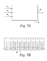
- FIG. 7A is an exemplary variable transport delay block in accordance with one aspect of the present invention.
- FIG. 7B is an exemplary lookup table dataset for use with an embodiment of the present invention.
- FIG. 8 is an exemplary pipe for illustration purposes.
- FIG. 9 depicts an exemplary buffer 900 suitable for use with exemplary embodiments described herein.
- FIG. 10 is a flowchart depicting an exemplary method for removing data elements from the buffer 900 .
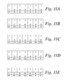
- FIGS. 11A-11E depict an exemplary buffer as data is added to the buffer and as the buffer is downsampled.
- FIG. 12 is a flowchart depicting an exemplary procedure for returning requested data to a requestor.
- FIG. 13 depicts an exemplary client/server configuration for requesting data from a buffer.
- FIG. 14 depicts exemplary rules for downsampling the data in the buffer.
- Exemplary embodiments provide methods, systems, and electronic media for managing data in a buffer by downsampling input buffer data to reduce the data density of the buffer.
- the buffer may hold a plurality of input data points associated with an index.
- the buffer may be associated with a data density that represents a logical distance between indices of adjacent input data points. That is, the data density represents a difference between element indexes for the data elements in the buffer. If the data elements are indexed by time, for example, then the data density may represent the average temporal distance between data elements that occur in temporal succession to each other. If the data elements are indexed by position, the data density may represent an average spatial distance between data elements that are located next to each other.
- the buffer is also associated with a capacity.
- a rule may be applied to the data buffer.
- Application of the rule may downsample the input data and reduce the data density of the buffer.
- Removed data points may be retrieved by deriving the removed data points from data points that remain in the buffer.
- intermediate data points may be removed so that the data density of the buffer is reduced, allowing the remaining values in the buffer to be spread out. That is, the element indexes of the elements in the buffer are more sparse or less dense after the data points are removed than before the data points are removed.
- the removed data points may then be extrapolated from the information stored in the buffer by deriving/interpolating the removed data points from the existing data points.
- the ability to reduce the data density of the buffer may be particularly useful in the context of the modeling of physical systems involving the calculation of transport delays, because transport delays are often stored in buffers and are particularly amenable to interpolation.
- Models of physical systems that use transport delays include models of transportation systems, airports, or conveyor belt arrangements. These transport delays may be best viewed as the time required for a material to go through a buffer of know size at a known speed.
- the simplest forms of transport delays are exhibited by a constant delay assigned to a signal which results in the delivery of the input signal at a fixed time in the future. In situations where the speed of material transfer through the buffer is constant, a variable time delay may be computed.
- variable time delay is best exhibited by example.
- a common instance of variable time delay is seen in the flow of an incompressible fluid through a pipe with an output located at length L distance away from the input.
- This length L can be best understood as a buffer between input and output.
- t d there will be a time delay t d determined by the length of the transportation and the speed of the transportation.
- the speed of the transportation i.e. the fill rate of the buffer
- v o (t) the speed at the outlet
- v i (t) and v o (t) are equal, as the fluid traversing the length L is incompressible.
- input u i and output u o which denote specific properties of the transported material, such as temperature at the inlet and outlet.
- FIGS. 1 through 6 illustrate an example embodiment of a variable transport delay according to the present invention.
- FIGS. 1 through 6 illustrate an example embodiment of a variable transport delay according to the present invention.
- FIG. 1 depicts a conventional variable time delay block 10 as understood in the prior art.
- This variable time delay block 10 can be used in conjunction with a graphical modeling environment, such as the Simulink® block diagram environment offered by The MathWorks, Inc. of Natick, Mass.
- a graphical modeling environment such as the Simulink® block diagram environment offered by The MathWorks, Inc. of Natick, Mass.
- the Variable time delay block 10 includes an input port 12 and an output port 14 .
- a signal provided to the input port 12 is delayed by a specific time prior to delivery to the output port 14 .
- This delay time 16 is user configurable.
- the block When used within a block diagram modeling environment, at the start of the simulation, the block outputs the input signal parameter provided to the input port 12 until the simulation time exceeds the preconfigured time delay parameter 16 , when the block begins generating the delayed input.
- the time delay parameter must be nonnegative.
- This conventional time delay stores input points and simulation times during a simulation in a buffer whose initial size is user defined.
- the block allocates additional memory and Simulink® displays a message after the simulation that indicates the total buffer size needed. Because allocating memory slows down the simulation, this parameter value must be defined carefully if simulation speed is an issue. For long time delays, this block might use a large amount of memory, particularly for a dimensionalized input.
- FIG. 2 is an illustrative example of the variable transport delay 20 of an embodiment of the present invention, which is used within a graphical block diagram environment, such as Simulink®.
- a graphical block diagram environment such as Simulink®.
- the variable transport delay 20 of the present invention includes an input 22 capable of receiving an input signal, and an output 24 capable of delivering an output signal to the modeling environment.
- an instantaneous delay signal 26 is associated with the variable transport delay block 20 . This instantaneous delay signal can be viewed as an estimated time of arrival, and is best understood by example.
- Equation 2 Equation 2
- variable transport delay generated in accordance with the present invention may be used in modeling conveyor belt delivery or products, automotive applications and traffic flow, for example.
- FIG. 3 is an illustrative example of the Variable Transport Delay 20 block of FIG. 2 , wherein illustrative internal steps of a sample Variable Transport Delay block 20 are illustrated for use in determining an output 24 that is delayed. These steps serve to illustrate a sample variable transport delay block and are not exclusive to the operation of a variable transport delay block used to generate a variable transport delay.
- a variable transport delay is ultimately calculated.
- the integration equation 2′ must first be solved. Following this step, u(t ⁇ t d ) can then be solved.
- the instantaneous delay T D is first inverted by the inversion element 32 , yielding
- the output of the inversion element 32 is passed to an integrator 34 .
- This integrator may take numerous forms, as understood by one skilled in the art.
- the integration equation 2′ can be solved using a stacked buffer of input u,t and the integration of
- FIG. 4 is an illustrative method for solving the output equation 38 using a lookup table arrangement. This illustrative method is not exclusive of the lookup table arrangement which may be employed with the current application. Numerous computation means, as understood by one skilled in the art, may be employed for use in calculating the value of:
- the time vector t is initially stored. As illustrated, the time vector t is stored in row 40 , wherein each column represents a different time step. In the present illustration the time step between columns is uniform, yet the present application may be practiced with non-uniform time steps.
- T D L v i ⁇ ( t ) .
- the value of x is then stored in row 42 of the lookup table at a variety of time steps, each designating an individual column. Additionally, the input value of u(t) is further stored in an individual row (row 44 ).
- lookup table arrangement is not the exclusive means by which the present invention may be practiced.
- numerous alternative means to calculate the integration result can be employed. Such means include, but are not limited to conversion of solving an integration equation, as set forth above, to the solving of a differential equation.
- L i ( t ) ⁇ L o ( t ) L
- L o ( t ) L i ( t ⁇ t d )
- Equation 2 has been converted into a differential equation, as illustrated in Equation 5, which may be solved using known computation techniques.
- the Simulink variable time block can be used to solve the differential equation of Equation 5.
- FIG. 5 is a flowchart illustrating the steps necessary in practicing one embodiment of the present invention.
- an initial buffer is first defined.
- This buffer is capable of storing buffer data, starting at an initial time and ending at a final time, in accordance with step 502 .
- Data stored by this buffer may take numerous forms and may include, but is not limited to, velocity, acceleration data or mass flow data.
- initial and final buffer data may be input and output velocity data.
- an instantaneous time delay is computed in accordance with step 504 .
- This instantaneous time delay may be viewed as an estimated time of arrival as a material traverses a length beginning at an input and ending at an output. As set forth earlier, in view of the incompressible flow through a pipe example, the instantaneous delay
- T D L v i ⁇ ( t ) .
- the calculation of instantaneous delay may occur using various means, including but not limited to computer based solutions. Following calculation of instantaneous delay in accordance with step 504 the instantaneous delay is integrated to generate a variable transport delay 506 . Integration of this instantaneous delay can occur using computer based integration means, such as interpolation using a lookup table, or may occur following the conversion of the integral into a differential equation.
- FIG. 6 is an exemplary computing device 600 suitable for practicing the illustrative embodiment of the present invention, which provides a block diagram environment.
- the computing device 600 is intended to be illustrative and not limiting of the present invention.
- the computing device 600 may take many forms, including but not limited to a workstation, server, network computer, quantum computer, optical computer, bio computer, Internet appliance, mobile device, a pager, a tablet computer, and the like.
- the computing device 600 may be electronic and include a Central Processing Unit (CPU) 610 , memory 620 , storage 630 , an input control 640 , a modem 650 , a network interface 660 , a display 670 , etc.
- the CPU 610 controls each component of the computing device 600 to provide the block diagram environment and to apply a coding standard to a block diagram in the block diagram environment.
- the memory 620 temporarily stores instructions and data and provides them to the CPU 610 so that the CPU 610 operates the computing device 600 and runs the block diagram environment.
- the storage 630 usually contains software tools for applications.
- the storage 630 includes, in particular, code 631 for the operating system (OS) of the device 600 , code 632 for applications running on the operation system including applications for providing the block diagram environment, and data 633 for block diagrams created in the block diagram environment and for one or more coding standards applied to the block diagrams.
- OS operating system
- the input control 640 may interface with a keyboard 680 , a mouse 690 , and other input devices.
- the computing device 600 may receive through the input control 640 input data necessary for creating block diagrams, such as the selection of the attributes and operations of component blocks in the block diagrams.
- the computing device 600 may also receive input data for applying a coding standard to a block diagram, such as data for selecting the coding standard, data for customizing the coding standard, data for correcting the violation of the coding standard in the block diagram, etc.
- the computing device 600 may display in the display 670 user interfaces for the users to edit the block diagrams.
- the computing device 600 may also display other user interfaces, such as a user interface for selecting a modeling standard, a user interface for customizing the modeling standard, a user interface for displaying a corrected block diagram that removes the violation of the modeling standard, etc.
- FIG. 7A is an embodiment of a variable transport delay block for use in settings wherein the aforementioned parameter “L” is variable, as opposed to a constant value which was assumed for the prior analysis.
- variable transport delay block includes three input which are used to generate a single output.
- an input signal “y” 72 , a velocity variable “v” 74 and a length variable “L” 76 are each provided to the variable transport delay block 70 .
- Equation 6 of the present embodiment may be solved using a similar method wherein buffer data is stored for use in interpolation of a final result.
- the storage of buffer data in accordance with the present embodiment requires the storage of two data sets of buffer data, namely velocity v(t) and Length L(t) data.
- FIG. 7B An illustrative lookup table including the variable L and the value of L at variable times 79 is illustrated in FIG. 7B .
- This output 78 may be delivered to a graphical block diagram model environment for use in subsequent calculation as understood by one skilled in the art.
- L is a parameter associated with the variable transport delay block as opposed to the explicit input illustrated in FIG. 7B .
- L is a parameter associated with the variable transport delay block as opposed to the explicit input illustrated in FIG. 7B .
- L is a parameter associated with the variable transport delay block as opposed to the explicit input illustrated in FIG. 7B .
- numerous pieces of information may be further associated with the parameter. For example, not only the value of a parameter may be specified, but also other information about the parameter, such as the parameter's purpose, its dimensions, its minimum and maximum values, etc.
- the above-described values may be stored in a buffer, such as the buffer 900 of FIG. 9 .
- the buffer 900 may be, for example, an array, matrix, or linked list.
- the buffer 900 is merely exemplary. More or fewer values and/or fields may be stored in the buffer 900 than are illustrated in FIG. 9 .
- the buffer 900 may take any form suitable for storing a plurality of data values and/or associated indices for the data values.
- the buffer 900 may include a field for the buffer index 910 of each of the data elements stored in the buffer.
- the buffer 900 may use zero based indexing, wherein the index of the i th element in the buffer is i ⁇ 1 (for example, the 1 st data element in the buffer is at buffer index 0).
- the buffer index 910 need not be explicitly stored in the buffer 900 for each (or any) data element. Rather, if the size s (in bytes) of the data elements in the buffer is known, then the i th data element in the buffer 900 may be found by starting from the beginning of the buffer 900 and moving into the buffer by (i ⁇ 1)*s bytes.
- the buffer 900 may further include a field that represents an element index 920 for a data element in the buffer.
- the element index 920 may be, for example, a temporal, spatial, or logical specification of the data element (e.g., a time or a location at which the data element was acquired).
- the element index 920 is separate from the buffer index 910 . Whereas the buffer index 910 represents the position of a particular data element in the buffer, the element index 920 may represent the position of a data element with respect to other data elements.
- the first data element has a buffer index 910 of 0, and an element index 920 of 0.1.
- the second data element has a buffer index 910 of 1, and an element index 920 of 0.4.
- the buffer 900 may include a field that represents a data value 930 for a data element in the buffer.
- the data value 930 may represent a data value obtained at the temporal, spatial, or logical location identified by the element index 920 .
- the element index 920 may represent a time t i at which a certain data point is collected.
- the data value 930 may represent a response v i of the model obtained at the time t i .
- the data value 930 may represent a variable transport delay representative of delayed data provided to the buffer.
- the variable transport delay may be used by a dynamic system represented in a model by one or more differential equations. As described in more detail above, variable transport delay represents an amount of delay incurred when something, such as a physical object or data, transits a certain physical or logical distance at a non-constant velocity.
- the variable transport delay may be determined by identifying an initial time at which one of the input data points starts and an ending time at which the one of the input data points ends, and calculating an instantaneous time delay using the initial time, the ending time and the input data point.
- the instantaneous time delay may be integrated, and the integrated instantaneous time delay may be assigned as the variable transport delay.
- a buffer such as the buffer 900 , typically has a finite capacity.
- the buffer 900 includes storage space for a number n of data elements, where n is the capacity of the buffer in terms of storable units (i.e., data elements).
- the data elements may be, for example, individual values such as integers or floating point numbers.
- the data elements also may be data structures representing combinations of values, such as arrays or matrixes (as shown, for example, in FIG. 7B ).
- the buffer 900 may be associated with a total capacity that is dependent on the size of the data elements contained in the buffer. For example, if the size allocated to each data element in the buffer is represented by s, then the total capacity of the buffer 900 (in terms of bytes) may be thought of as n*s.
- the buffer 900 may be “downsampled.” Downsampling the buffer 900 may involve reducing a data density of the buffer 900 by removing data values from the buffer 900 , such as intermediate data values (i.e., data values that are between the first and last data value in the buffer). Alternatively or in addition to the above, the first and/or last data value may be removed.
- the data density of the buffer may be thought of as the average distance between adjacent element indexes 920 of the elements in the buffer.
- the average distance between the times in this sequence is 1 second (this value being the average distance between adjacent element indexes 920 in the buffer).
- the distance between the first element index 920 and the second element index 920 is 4 seconds.
- the distance between the second element index and the third element index is 2 seconds.
- the distance between the third element index and the fourth element index is 4 seconds.
- the average distance between the times in this example is 3.333 seconds (the average of 4 seconds, 2 seconds, and 4 seconds).
- Downsampling the buffer 900 to reduce the data density of the buffer may be employed when the buffer is at or near the buffer's maximum capacity. This may provide more room in the buffer 900 to store additional data elements.
- FIG. 10 depicts an exemplary procedure for removing data elements from the buffer 900 .
- the buffer may be operated upon in some manner. For example, a request may be made to store or retrieve data from the buffer. It should be noted that downsampling may occur during an operation on the buffer, or may occur before or after the operation takes place.
- the buffer may be determined if the buffer is at or near capacity.
- the buffer is at capacity when the buffer is capable of storing n data elements and the buffer currently stores n data elements.
- the buffer is considered near capacity when the buffer approaches the capacity and is within a predetermined threshold range of the capacity. For example, if the threshold range is m data elements, then the buffer may be considered near capacity when the buffer currently stores n-m data elements.
- whether the buffer is at or near capacity may be determined by consulting a counter variable.
- the counter variable is initialized at 0 and is incremented each time data is written to the buffer.
- the buffer is determined to be at or near capacity. If the buffer is downsampled as described below with respect to step 1030 , the counter variable may be decremented once for each value removed from the buffer. Thus, the counter variable always reflects the number of data elements currently stored in the buffer.
- the buffer may be downsampled to reduce the data density of the buffer.
- the entire buffer could be downsampled, or only a portion of the buffer may be downsampled while the remainder of the buffer is left untouched. This may be useful, for example, if relatively recent data values in the buffer are to be left intact while some or all older data values in the buffer can be removed.
- downsampling of the buffer may be triggered when the buffer is at or near capacity. However, downsampling may be triggered under other conditions as well, such as at predetermined points in time during the modeling process. Furthermore, the downsampling may be triggered dynamically (e.g., different triggering events may trigger the downsampling through the course of a simulation, as in the case where a different value for m is applied at different points in the simulation).
- FIG. 11A an empty buffer is provided.
- the buffer has seven buffer indices labeled zero through six. Each buffer index holds a data element associated with an element index and an element value.
- FIG. 11A depicts the buffer after a single data element has been added at buffer index 0.
- the first data element has an element index of 5 and a value of 25. This may signify, for example, that an output value of “25” was generated from a model at time 5 .
- a second data element has been added to the buffer.
- the second data element is stored at buffer index 1 and is associated with an element index of 10 and an element value of 100. This may indicate, for example, that a value of 100 was generated by the model at time 10 .
- the average distance between element indexes in FIG. 11B is 5, because only two values are present in the buffer, and the element indexes of the elements are separated from each other by 5.
- FIG. 11C depicts the buffer after seven data elements have been added. Because the buffer is capable of storing only seven elements, the buffer is now at capacity. In FIG. 11C , the average distance between element indexes is 5 because the average difference between adjacent data elements is 5. Thus, the data density of FIG. 11C is the equivalent to the data density in FIG. 11B .
- the buffer may be downsampled to reduce the data density of the buffer. For example, as described above with respect to FIG. 10 , every k th data element may be removed from the buffer.
- FIG. 11D every 2 nd data element has been removed from the buffer of FIG. 11C . Accordingly, intermediate data elements having the element indexes 10 , 20 , and 30 have been removed. As a result, the data density has been reduced because the average distance between adjacent element indexes in FIG. 11D is now 10 (whereas the average distance of FIG. 11C was 5). Thus, the data density of FIG. 11D is less than the data density of FIG. 11C .
- the buffer slots from the data elements that were eliminated from the buffer may be left blank and may be filled with new data elements as the new elements are added to the buffer.
- the element indexes of the data elements may be out-of-order in the buffer.
- the average value of adjacent element indexes should be used.
- the buffer may either be rearranged in order or searched to determine which element indexes are adjacent to each other. So, for example, if the buffer includes the out-of-order element indexes “1-5-3-7,” the average distance is 2 because the distance from each element to each adjacent element (i.e., from 1 to 3, from 3 to 5, and from 5 to 7) is 2.
- the buffer of FIG. 11D has freed three empty data slots, at buffer indexes 4, 5, and 6. Accordingly, additional data may be stored in the buffer, as shown in FIG. 11E .
- a new data point having an element index of 40 has been added at buffer index 4.
- the average distance between adjacent element indexes in FIG. 11E is now 8.75, and hence the data density has increased from FIG. 11D to FIG. 11E . This is an acceptable increase, since the data density must only decrease at the time that the buffer is downsampled.
- Data may be requested from the buffer before or after the buffer is downsampled. In some cases, the data will be present in the buffer but in others the data will have been removed during the downsampling process. However, the removed data values may still be estimated by interpolating between data values that still exist in the buffer, as described below with respect to FIG. 12 .
- FIG. 12 is a flowchart depicting an exemplary procedure for returning a requested value to a requestor.
- a request for data may be received at the buffer.
- the request may identify, for example, an element index of the requested data and may request the element value associated with that element index.
- the buffer may be inspected to determine whether an element associated with the identified element index is present in the buffer. If so, processing proceeds to step 1230 and the requested data element is simply looked up in the buffer. Processing then proceeds to step 1250 and the requested data is returned. If the element does not exist in the buffer at step 1220 , processing proceeds to step 1240 .
- step 1220 it may determined that the requested data element is not stored in the buffer. This may be because the requested data point was downsampled and removed from the buffer, or because the requested data point never existed in the buffer. In either case, it may still be possible to derive the requested data from the data that exists in the buffer.
- the missing data values may be interpolated by determining a relationship between the element values and the element indexes stored in the buffer. For example, a regression analysis may be performed in order to determine an acceptable approximate formula that relates the element values and the element indexes of the buffer. For example, different equations relating the element values to the element indexes (e.g., linear equations, polynomial equations, etc.) may be applied to the data in the buffer until an error value indicating a fitness of the equation for modeling the data is reduced below a predetermined threshold.
- the fitness may be represented, for example, by any error metric such as a least-squares metric.
- the relationship may be applied to determine the estimated element value associated with the requested element index. Processing then proceeds to step 1250 .
- the requested data is returned.
- One or more entities may serve as requesting entities that request data from the buffer in accordance with the procedure described above.
- the buffer may be stored on the requesting entity, as in the case where a single computer maintains the buffer and analyzes data from the buffer.
- FIG. 13 depicts an exemplary client/server configuration for requesting data from a buffer.
- a central server 1300 stores and maintains a buffer 1310 .
- the server 1300 may be, for example, a personal computer, a dedicated mainframe server, a mobile computer such as a tablet or phone, or a custom electronic device.
- Requesting entities 1320 , 1330 , 1340 , 1350 may request data from the buffer 1310 by sending requests to the server 1300 . Additionally, the requesting entities 1320 , 1330 , 1340 , 1350 may request that data be added to the buffer by sending an appropriate data_add request to the server 1300 .
- the server 1300 may be tasked with managing access to the buffer 1310 and with maintaining data integrity in the buffer 1310 .
- the server 1300 may detect when the buffer 1310 is at or near capacity, and may apply one or more rules to downsample the data. Examples of such rules are shown in FIG. 14 .
- rules 1400 may include one or more instructions for downsampling the buffer.
- the rules may be programmatically determined and/or user-defined.
- the buffer may be downsampled according to the same rule each time, or the downsampling may be context-dependent, applying a different rule depending on conditions in the buffer, the server or the requesting entities.
- k may be any integer value from 2 to n (the maximum capacity of the buffer). The lower the value of k, the more space will be freed from the buffer. Accordingly, the value of k may be either predetermined, or may be determined dynamically depending on conditions related to the buffer. For example, if the buffer stores data associated with a simulation of a model and the simulation is nearing its end, then it is unlikely that a large amount of additional data will need to be stored in the buffer before the simulation is finished. Accordingly, a relatively high value of k may be selected so that only a few data points are removed from the buffer.
- a small value of k may be selected in order to remove more values from the buffer and therefore further increase the storage available in the buffer.
- two or more values may be used for k in the same downsampling procedure (e.g., “remove every 2 nd value and every 5 th value,” or “begin by removing every 2 nd value and then remove every 3 rd value,” etc.).
- Another rule 1420 is to remove the least-requested data. If this rule is selected, a counter may be associated with each data element. The counter may identify how many times the data element has been requested. When the buffer must be downsampled, the counter may be consulted to determine which data elements are used the least. These data elements may be removed to make room for future data elements.
- the counter may reflect the number of times that the single requesting entity has requested the data. Alternatively, if there are multiple requesting entities, then the counter may reflect the cumulative number of times that the data element has been requested by all the requesting entities. In some embodiments, some requesting entities may be deemed to be more or less important than other requesting entities. Accordingly, requests from the more important requesting entities may be weighted in order to preserve the data requested most often by the more important requesting entities.
- a further rule 1430 is to minimize the change in data density when the buffer is downsampled. For example, if the buffer includes element indexes “1-2-3-10,” then removing the value “10” causes the average distance between element indexes to go from an original value of 3 to a new value of 1. On the other hand, removing the value “2” causes the average distance to change from 3 to 4.5. Accordingly, in this example, the value 2 would be removed.
- Minimizing the change in density may, in some situations, make it easier to interpolate values for data that is removed.
- a requesting entity requests the data associated with the element index “10” after the data element has been removed.
- the existing data (“1-2-3”) must be used to extrapolate a value that is more than three times the maximum value stored in the buffer.
- this extrapolation may be problematic.
- the value “2” is requested after the value “2” is removed, it is simpler to interpolate between the values of “1” and “3,” which continue to be stored in the buffer.
- space can be freed in a buffer so that additional data may be added to the buffer.
- the data is removed in such a way (i.e., by reducing the data density of the buffer rather than simply removing data from the front or back of the buffer) that the removed data can still be interpolated from the data remaining in the buffer.
Landscapes
- Engineering & Computer Science (AREA)
- Physics & Mathematics (AREA)
- Theoretical Computer Science (AREA)
- Mathematical Physics (AREA)
- Data Mining & Analysis (AREA)
- General Physics & Mathematics (AREA)
- Mathematical Analysis (AREA)
- Mathematical Optimization (AREA)
- Computational Mathematics (AREA)
- Pure & Applied Mathematics (AREA)
- Databases & Information Systems (AREA)
- Software Systems (AREA)
- General Engineering & Computer Science (AREA)
- Algebra (AREA)
- Complex Calculations (AREA)
Abstract
Description
v i(t)=v o(t)
L i(t)−L i(t−t d)=L •
L=∫t-td t v i(τ)dτ (Equation 1)
Normalizing
wherein:
such that TD is called instantaneous delay or can be understood as estimated time of arrival. In view of this,
The use of a pipe with an incompressible flow is solely for illustrative purposes and as such not intended to be limiting on scope of the present invention. For example, the variable transport delay generated in accordance with the present invention may be used in modeling conveyor belt delivery or products, automotive applications and traffic flow, for example.
The output of the
The output equation 38 y=u(t−td), where td is determined by equation (2′), such that a variable
set forth prior. In the present embodiment, as illustrated in
wherein
Further note that
x(7)47−x(2)48=2.3−1.2=1.1>1 and
x(7)47−x(3)48=2.3−1.4=0.9<1
it is clear that:
t(2)50<t−td<t(3)→
0.5<t−td<0.6.
Using the method of interpolation it can be determined that t−td=0.55. This interpolation information can further be used to find u(0.55). As u(0.5)=1.6 (52) and u (0.6)=0.5 (53) the value of u(0.55) can be interpolated. This output may then be passed to a graphical block diagram modeling environment for use in further simulation.
L i(t)=∫t
while the conservation variable of the outlet can be defined as:
L o(t)=∫t
In view of this,
L i(t)−L o(t)=L, and
L o(t)=L i(t−t d), therefore:
v i(t)=v o(t)
L i(t)−L i(t−t d)=L • (Equation 3)
Following the differentiation of Equation (3) with respect to t yields:
Wherein vi is the transport speed.
The calculation of instantaneous delay may occur using various means, including but not limited to computer based solutions. Following calculation of instantaneous delay in accordance with
L(t)=∫t-t
wherein the speed of the transportation is denoted as v(t) and the delay time td is the delay time parameter needed.
Absent the normalization process employed in a setting wherein the “L” parameter is constant,
Rewriting
L(t)−∫t-t
wherein the solution to:
L(t)−∫t
and
L(t)−∫t
can be found. In view of this,
t k <t−t d <t k+1
Using an interpolation approach, in accordance with the setting wherein “L” is constant, the value of t−td. can be determined. This interpolation will require the storage of an additional variable, namely L(t) for use in the interpolation of t−td. An illustrative lookup table including the variable L and the value of L at
u=y(t−t d).
This
Claims (20)
Priority Applications (1)
| Application Number | Priority Date | Filing Date | Title |
|---|---|---|---|
| US13/470,891 US8700366B1 (en) | 2005-09-06 | 2012-05-14 | Variable transport delay modelling mechanism |
Applications Claiming Priority (3)
| Application Number | Priority Date | Filing Date | Title |
|---|---|---|---|
| US11/221,160 US7835889B1 (en) | 2005-09-06 | 2005-09-06 | Variable transport delay modelling mechanism |
| US12/907,631 US8180608B1 (en) | 2005-09-06 | 2010-10-19 | Variable transport delay modeling mechanism |
| US13/470,891 US8700366B1 (en) | 2005-09-06 | 2012-05-14 | Variable transport delay modelling mechanism |
Related Parent Applications (1)
| Application Number | Title | Priority Date | Filing Date |
|---|---|---|---|
| US12/907,631 Continuation-In-Part US8180608B1 (en) | 2005-09-06 | 2010-10-19 | Variable transport delay modeling mechanism |
Publications (1)
| Publication Number | Publication Date |
|---|---|
| US8700366B1 true US8700366B1 (en) | 2014-04-15 |
Family
ID=50441538
Family Applications (1)
| Application Number | Title | Priority Date | Filing Date |
|---|---|---|---|
| US13/470,891 Expired - Lifetime US8700366B1 (en) | 2005-09-06 | 2012-05-14 | Variable transport delay modelling mechanism |
Country Status (1)
| Country | Link |
|---|---|
| US (1) | US8700366B1 (en) |
Cited By (1)
| Publication number | Priority date | Publication date | Assignee | Title |
|---|---|---|---|---|
| US10565328B2 (en) | 2015-07-20 | 2020-02-18 | Samsung Electronics Co., Ltd. | Method and apparatus for modeling based on particles for efficient constraints processing |
Citations (6)
| Publication number | Priority date | Publication date | Assignee | Title |
|---|---|---|---|---|
| US4550318A (en) * | 1982-02-03 | 1985-10-29 | The Johns Hopkins University | Retrospective data filter |
| US20020064171A1 (en) | 1998-10-08 | 2002-05-30 | Adtran, Inc. | Dynamic delay compensation for packet-based voice network |
| US6732064B1 (en) | 1997-07-02 | 2004-05-04 | Nonlinear Solutions, Inc. | Detection and classification system for analyzing deterministic properties of data using correlation parameters |
| US20050259754A1 (en) | 2004-05-18 | 2005-11-24 | Jin-Meng Ho | Audio and video clock synchronization in a wireless network |
| US20080021679A1 (en) * | 2006-07-24 | 2008-01-24 | Ati Technologies Inc. | Physical simulations on a graphics processor |
| US7495450B2 (en) | 2002-11-19 | 2009-02-24 | University Of Utah Research Foundation | Device and method for detecting anomolies in a wire and related sensing methods |
-
2012
- 2012-05-14 US US13/470,891 patent/US8700366B1/en not_active Expired - Lifetime
Patent Citations (6)
| Publication number | Priority date | Publication date | Assignee | Title |
|---|---|---|---|---|
| US4550318A (en) * | 1982-02-03 | 1985-10-29 | The Johns Hopkins University | Retrospective data filter |
| US6732064B1 (en) | 1997-07-02 | 2004-05-04 | Nonlinear Solutions, Inc. | Detection and classification system for analyzing deterministic properties of data using correlation parameters |
| US20020064171A1 (en) | 1998-10-08 | 2002-05-30 | Adtran, Inc. | Dynamic delay compensation for packet-based voice network |
| US7495450B2 (en) | 2002-11-19 | 2009-02-24 | University Of Utah Research Foundation | Device and method for detecting anomolies in a wire and related sensing methods |
| US20050259754A1 (en) | 2004-05-18 | 2005-11-24 | Jin-Meng Ho | Audio and video clock synchronization in a wireless network |
| US20080021679A1 (en) * | 2006-07-24 | 2008-01-24 | Ati Technologies Inc. | Physical simulations on a graphics processor |
Non-Patent Citations (2)
| Title |
|---|
| Casetti, C. et al., "A Framework for the Analysis of Adaptive Voice over IP," ICC 2000, IEEE International Conference on Communications, vol. 2:821-826 (2000). |
| Dermanovic, B. et al., "Modeling of Transport Delay on ETHERNET Communication Networks," IEEE MELECON, pp. 367-370 (2004). |
Cited By (1)
| Publication number | Priority date | Publication date | Assignee | Title |
|---|---|---|---|---|
| US10565328B2 (en) | 2015-07-20 | 2020-02-18 | Samsung Electronics Co., Ltd. | Method and apparatus for modeling based on particles for efficient constraints processing |
Similar Documents
| Publication | Publication Date | Title |
|---|---|---|
| US7676522B2 (en) | Method and system for including data quality in data streams | |
| CN103635896B (en) | The method and system of prediction user's navigation event | |
| US7676523B2 (en) | Method and system for managing data quality | |
| CN110347651B (en) | Cloud storage-based data synchronization method, device, equipment and storage medium | |
| US10650559B2 (en) | Methods and systems for simplified graphical depictions of bipartite graphs | |
| CN110674121A (en) | Cache data cleaning method, device, equipment and computer readable storage medium | |
| CN102884526B (en) | Show items in the app window | |
| US9594839B2 (en) | Methods and systems for load balancing databases in a cloud environment | |
| JP2022547433A (en) | Empirical provision of data privacy using noise reduction | |
| Chabini | Analytical dynamic network loading problem: Formulation, solution algorithms, and computer implementations | |
| Spears et al. | Analyzing GAs Using Markov Models with Semantically Ordered and Lumped States. | |
| CN107168643A (en) | A kind of date storage method and device | |
| Riska et al. | M/G/1-type Markov processes: A tutorial | |
| US8700366B1 (en) | Variable transport delay modelling mechanism | |
| Campos Pinto et al. | Convergence of a linearly transformed particle method for aggregation equations | |
| CN115525793A (en) | Method, system and storage medium realized by computer | |
| CN106294503B (en) | Data dynamic storage method, device and computing equipment | |
| US20080005052A1 (en) | Aggregation-specific confidence intervals for fact set queries | |
| US10210206B2 (en) | Optimization of a plurality of table processing operations in a massive parallel processing environment | |
| Wobbes et al. | Comparison and unification of material-point and optimal transportation meshfree methods: E. Wobbes et al. | |
| US12430174B2 (en) | Systems and methods for memory management in big data applications | |
| Wolff et al. | Asynchronous collision integrators: Explicit treatment of unilateral contact with friction and nodal restraints | |
| WO2011131248A1 (en) | Method and apparatus for losslessly compressing/decompressing data | |
| JP2007102501A (en) | Method and apparatus for calculating degree of association between words | |
| JP2007128382A (en) | Performance prediction method of cluster system and device |
Legal Events
| Date | Code | Title | Description |
|---|---|---|---|
| AS | Assignment |
Owner name: THE MATHWORKS, INC., MASSACHUSETTS Free format text: ASSIGNMENT OF ASSIGNORS INTEREST;ASSIGNORS:ZHANG, FU;YEDDANAPUDI, MURALI;SIGNING DATES FROM 20051020 TO 20051024;REEL/FRAME:028795/0325 |
|
| STCF | Information on status: patent grant |
Free format text: PATENTED CASE |
|
| CC | Certificate of correction | ||
| FEPP | Fee payment procedure |
Free format text: PAYOR NUMBER ASSIGNED (ORIGINAL EVENT CODE: ASPN); ENTITY STATUS OF PATENT OWNER: LARGE ENTITY |
|
| MAFP | Maintenance fee payment |
Free format text: PAYMENT OF MAINTENANCE FEE, 4TH YEAR, LARGE ENTITY (ORIGINAL EVENT CODE: M1551) Year of fee payment: 4 |
|
| MAFP | Maintenance fee payment |
Free format text: PAYMENT OF MAINTENANCE FEE, 8TH YEAR, LARGE ENTITY (ORIGINAL EVENT CODE: M1552); ENTITY STATUS OF PATENT OWNER: LARGE ENTITY Year of fee payment: 8 |
|
| FEPP | Fee payment procedure |
Free format text: MAINTENANCE FEE REMINDER MAILED (ORIGINAL EVENT CODE: REM.); ENTITY STATUS OF PATENT OWNER: LARGE ENTITY |