US8508226B2 - Method and magnetic resonance system to reduce distortions in diffusion imaging - Google Patents
Method and magnetic resonance system to reduce distortions in diffusion imaging Download PDFInfo
- Publication number
- US8508226B2 US8508226B2 US13/020,302 US201113020302A US8508226B2 US 8508226 B2 US8508226 B2 US 8508226B2 US 201113020302 A US201113020302 A US 201113020302A US 8508226 B2 US8508226 B2 US 8508226B2
- Authority
- US
- United States
- Prior art keywords
- magnetic resonance
- diffusion
- image
- specific
- resonance data
- Prior art date
- Legal status (The legal status is an assumption and is not a legal conclusion. Google has not performed a legal analysis and makes no representation as to the accuracy of the status listed.)
- Active, expires
Links
- 238000000034 method Methods 0.000 title claims abstract description 112
- 238000009792 diffusion process Methods 0.000 title claims abstract description 79
- 238000003384 imaging method Methods 0.000 title claims abstract description 25
- 238000012937 correction Methods 0.000 claims abstract description 96
- 238000005259 measurement Methods 0.000 claims abstract description 77
- 230000009466 transformation Effects 0.000 claims description 99
- 230000006870 function Effects 0.000 claims description 90
- 238000000844 transformation Methods 0.000 claims description 55
- 238000012360 testing method Methods 0.000 claims description 16
- PXFBZOLANLWPMH-UHFFFAOYSA-N 16-Epiaffinine Natural products C1C(C2=CC=CC=C2N2)=C2C(=O)CC2C(=CC)CN(C)C1C2CO PXFBZOLANLWPMH-UHFFFAOYSA-N 0.000 claims description 13
- 230000001419 dependent effect Effects 0.000 claims description 6
- 230000004913 activation Effects 0.000 claims 2
- 230000001131 transforming effect Effects 0.000 claims 1
- 238000005457 optimization Methods 0.000 description 17
- 230000000875 corresponding effect Effects 0.000 description 11
- 238000006073 displacement reaction Methods 0.000 description 6
- 238000012545 processing Methods 0.000 description 6
- 238000003702 image correction Methods 0.000 description 5
- 238000013519 translation Methods 0.000 description 5
- 230000008901 benefit Effects 0.000 description 4
- 238000004364 calculation method Methods 0.000 description 4
- 238000013461 design Methods 0.000 description 4
- 230000000694 effects Effects 0.000 description 4
- 239000011159 matrix material Substances 0.000 description 4
- 238000000926 separation method Methods 0.000 description 4
- 230000002596 correlated effect Effects 0.000 description 3
- 238000011156 evaluation Methods 0.000 description 3
- 238000000691 measurement method Methods 0.000 description 3
- 238000012986 modification Methods 0.000 description 3
- 230000004048 modification Effects 0.000 description 3
- 238000001208 nuclear magnetic resonance pulse sequence Methods 0.000 description 3
- 230000002123 temporal effect Effects 0.000 description 3
- 230000006978 adaptation Effects 0.000 description 2
- 238000004458 analytical method Methods 0.000 description 2
- 238000013459 approach Methods 0.000 description 2
- 230000005540 biological transmission Effects 0.000 description 2
- 238000006243 chemical reaction Methods 0.000 description 2
- 238000010586 diagram Methods 0.000 description 2
- 238000013213 extrapolation Methods 0.000 description 2
- 230000006872 improvement Effects 0.000 description 2
- 238000009434 installation Methods 0.000 description 2
- 230000001788 irregular Effects 0.000 description 2
- 238000012423 maintenance Methods 0.000 description 2
- 239000000463 material Substances 0.000 description 2
- 238000007619 statistical method Methods 0.000 description 2
- 230000001133 acceleration Effects 0.000 description 1
- 230000004075 alteration Effects 0.000 description 1
- 230000006399 behavior Effects 0.000 description 1
- 238000007906 compression Methods 0.000 description 1
- 230000006835 compression Effects 0.000 description 1
- 238000010219 correlation analysis Methods 0.000 description 1
- 230000007423 decrease Effects 0.000 description 1
- 238000009795 derivation Methods 0.000 description 1
- 238000011161 development Methods 0.000 description 1
- 238000003745 diagnosis Methods 0.000 description 1
- 238000009826 distribution Methods 0.000 description 1
- 230000007717 exclusion Effects 0.000 description 1
- 230000003631 expected effect Effects 0.000 description 1
- 238000009472 formulation Methods 0.000 description 1
- 238000003780 insertion Methods 0.000 description 1
- 230000037431 insertion Effects 0.000 description 1
- 230000002452 interceptive effect Effects 0.000 description 1
- 238000004519 manufacturing process Methods 0.000 description 1
- 239000000203 mixture Substances 0.000 description 1
- 238000012544 monitoring process Methods 0.000 description 1
- 238000010606 normalization Methods 0.000 description 1
- 230000008520 organization Effects 0.000 description 1
- 230000008569 process Effects 0.000 description 1
- 230000005855 radiation Effects 0.000 description 1
- 230000009467 reduction Effects 0.000 description 1
- 230000004044 response Effects 0.000 description 1
- 238000010187 selection method Methods 0.000 description 1
- 230000035945 sensitivity Effects 0.000 description 1
- 230000003068 static effect Effects 0.000 description 1
Images


Classifications
-
- G—PHYSICS
- G01—MEASURING; TESTING
- G01R—MEASURING ELECTRIC VARIABLES; MEASURING MAGNETIC VARIABLES
- G01R33/00—Arrangements or instruments for measuring magnetic variables
- G01R33/20—Arrangements or instruments for measuring magnetic variables involving magnetic resonance
- G01R33/44—Arrangements or instruments for measuring magnetic variables involving magnetic resonance using nuclear magnetic resonance [NMR]
- G01R33/48—NMR imaging systems
- G01R33/54—Signal processing systems, e.g. using pulse sequences ; Generation or control of pulse sequences; Operator console
- G01R33/56—Image enhancement or correction, e.g. subtraction or averaging techniques, e.g. improvement of signal-to-noise ratio and resolution
- G01R33/561—Image enhancement or correction, e.g. subtraction or averaging techniques, e.g. improvement of signal-to-noise ratio and resolution by reduction of the scanning time, i.e. fast acquiring systems, e.g. using echo-planar pulse sequences
- G01R33/5615—Echo train techniques involving acquiring plural, differently encoded, echo signals after one RF excitation, e.g. using gradient refocusing in echo planar imaging [EPI], RF refocusing in rapid acquisition with relaxation enhancement [RARE] or using both RF and gradient refocusing in gradient and spin echo imaging [GRASE]
- G01R33/5616—Echo train techniques involving acquiring plural, differently encoded, echo signals after one RF excitation, e.g. using gradient refocusing in echo planar imaging [EPI], RF refocusing in rapid acquisition with relaxation enhancement [RARE] or using both RF and gradient refocusing in gradient and spin echo imaging [GRASE] using gradient refocusing, e.g. EPI
-
- G—PHYSICS
- G01—MEASURING; TESTING
- G01R—MEASURING ELECTRIC VARIABLES; MEASURING MAGNETIC VARIABLES
- G01R33/00—Arrangements or instruments for measuring magnetic variables
- G01R33/20—Arrangements or instruments for measuring magnetic variables involving magnetic resonance
- G01R33/44—Arrangements or instruments for measuring magnetic variables involving magnetic resonance using nuclear magnetic resonance [NMR]
- G01R33/48—NMR imaging systems
- G01R33/54—Signal processing systems, e.g. using pulse sequences ; Generation or control of pulse sequences; Operator console
- G01R33/56—Image enhancement or correction, e.g. subtraction or averaging techniques, e.g. improvement of signal-to-noise ratio and resolution
- G01R33/563—Image enhancement or correction, e.g. subtraction or averaging techniques, e.g. improvement of signal-to-noise ratio and resolution of moving material, e.g. flow contrast angiography
- G01R33/56341—Diffusion imaging
Definitions
- the present invention concerns a method to correct image distortions that can occur upon acquisition of diffusion-weighted magnetic resonance (MR) images of an examination subject, as well as a magnetic (MR) resonance system with which such a method can be implemented.
- MR diffusion-weighted magnetic resonance
- diffusion imaging multiple images are normally acquired with different diffusion directions and weightings, and are combined with one another.
- the strength of the diffusion weighting is usually defined by what is known as the “b-value”.
- the diffusion images with different diffusion directions and weightings, or the images combined therefrom can then be used for diagnostic purposes.
- Parameter maps with particular diagnostic significance for example, maps that reflect the “Apparent Diffusion Coefficient (ADC)” or the “Fractional Anisotropy (FA)”, can be generated by suitable combinations of the acquired, diffusion-weighted images.
- ADC Apparent Diffusion Coefficient
- FA Fractional Anisotropy
- Eddy current fields can disadvantageously be caused by the diffusion gradients, these eddy current fields in turn leading to image distortions having an appearance that depends both on the amplitude of the gradients (i.e. the diffusion weighting) and on their direction. If the acquired individual images are then combined with one another with no correction in order to generate (for example) the cited parameter maps, the distortions, which are different for every image, lead to incorrect associations of pixel information and therefore to errors (or at to a reduced precision) of the calculated parameters.
- eddy current-dependent distortions represent a particularly significant challenge, since a particularly high sensitivity (approximately 10 Hz per pixel in the phase coding direction) to static and dynamic field interference typically exists in EPI imaging, and high gradient amplitudes are specifically used here to adjust the diffusion gradients.
- Distortion parameters for M, S and T are therefore determined with the aid of the two adjustment measurements, i.e. the measurement of the reference image and the image with low diffusion weighting. Using an extrapolation relationship, the distortion parameters M, S and T that are determined in this way are then utilized for the correction of the actual diffusion-weighted usable MR images in which the b-value amounts to 1000 s/m 2 , for example. This method requires at least one adjustment measurement for each diffusion direction.
- An object of the present invention is to provide an improved method to reduce distortions in diffusion imaging, which method also takes interference fields with more complex spatial geometry into account in the correction and is nevertheless sufficiently robust and quick.
- a further object is to provide a magnetic resonance system that is designed to implement a more complex spatial geometry within the scope of the invention is an interference field geometry that goes beyond an affine transformation.
- At least one first measurement is thus initially implemented with a first diffusion weighting and at least one second measurement is initially implemented with a second diffusion weighting.
- these can hereby be different measurements.
- Analogous to the method from Bodammer et al. it is also similarly possible to implement the two measurements with identical diffusion direction and diffusion weighting but inverted polarity in order to thus arrive at different measurements.
- the first measurement typically serves purely as a reference or adjustment measurement.
- the diffusion-weighted and distorted images that are acquired in the second measurement can be used not only for the determination of the correction parameters (thus not only as an “adjustment measurement”), but also the images can be directly used for a diagnosis after the correction, for example.
- a direct registration of the diffusion-weighted diagnostic images to reference images thus occurs using the described method (non-linear transformation with system-specific distortion correcting function). Additional usable measurements are then no longer necessary since the second adjustment measurements themselves form the usable measurements.
- the first and second measurements in the method according to the invention are always used as adjustment measurements, they are designated as “adjustment measurements” in the following without limitation of the generality.
- system-specific as used herein encompasses the term “system type-specific”, meaning that information about the gradient coil design used in the system type or other structural information are used, for example.
- Correction parameters for correcting diffusion-weighted magnetic resonance images are determined by applying this system-specific distortion correcting function and on the basis of the adjustment measurements. This can ensue in a known manner, for example with an iterative optimization method by means of simplex maximization of a similarity function. For example, the similarity of an adjustment image from the one adjustment image is thereby assessed with a corresponding image from the second adjustment measurement on the basis of a measure of similarity, particularly preferably on the basis of the “Normalized Mutual Information” (NMI), is found in Peter E. Latham and Yasser Roudi (2009), Scholarpedia, 4(1): 1658 . In the iterative method the optimal correction parameters are then determined as variables (in particular coefficients) of the distortion correcting function.
- NMI Normalized Mutual Information
- a correction of the diffusion-weighted magnetic resonance images takes place on the basis of the correction parameters and with application of the distortion correcting function.
- the diffusion-weighted images that are acquired in the second adjustment measurement are used not only for the determination of the correction parameters but also as “usable images”, in this step these images from the second measurement are thus corrected on the basis of the correction parameters and using the distortion correcting function.
- this step can also already take place as a last adaptation step within the framework of the optimization method to determine the optimal correction parameter.
- a magnetic resonance system In addition to an image acquisition unit to acquire diffusion-weighted images of an examination subject and to implement at least the first measurement with a first diffusion weighting and at least the second method with a second diffusion weighting, a magnetic resonance system according to the invention requires a correction parameter determination unit.
- This correction parameter determination unit is fashioned so that during operation it determines a non-linear, system-specific distortion correcting function and then calculates the correction parameters to correct diffusion-weighted magnetic resonance images on the basis of the first and second measurements with application of the distortion correcting function.
- the magnetic resonance system according to the invention has an image correction unit to correct the diffusion-weighted magnetic resonance images on the basis of the correction parameters.
- the correction parameter determination unit and the image correction unit can thereby be arranged in a central controller of the magnetic resonance system or in a separate, downstream image processing unit—for example a workstation serving as an image monitoring and processing unit—to which the data from the adjustment measurement and the diffusion-weighted images are transmitted after the reconstruction.
- a separate, downstream image processing unit for example a workstation serving as an image monitoring and processing unit—to which the data from the adjustment measurement and the diffusion-weighted images are transmitted after the reconstruction.
- the method according to the invention or, respectively, the magnetic resonance system according to the invention has the advantage that on the on hand not only affine transformations but also significantly more complex geometries of the interference fields can be taken into account.
- the use of a system-specific distortion correcting function provides that the number of correction parameters to be determined keeps within a scope in which a robust and fast determination of the correction parameters is still possible.
- the distortion correcting function is additionally better adapted to the actual existing interference conditions than in previous methods, and therefore can lead to more precise corrections.
- the present invention also encompasses a magnetic resonance apparatus that is designed to implement the above-described method, and all embodiments thereof, with the same advantages described in connection with the above method.
- the determination of the system-specific distortion correcting function can thereby also be based on heuristic information. For example, for a specific system type it can turn out that interference fields of a first order and of a specific additional term of a higher order significantly occur upon shifting of a diffusion gradient in an x-direction. This knowledge can then directly serve to establish a system-specific distortion correcting function. Other system-specific information or, respectively, methods to establish the system-specific distortion correcting function can likewise be supplemented by such heuristic information.
- system-specific information preferably includes direct parameters of a field geometry occurring upon application of a gradient field in the relevant magnetic resonance system.
- the system-specific information can include to the greatest extent possible the complete mathematical description of this field geometry depending on the respective gradient field that is applied.
- a system-specific geometry of field disruptions is determined, in order to determine the system-specific distortion correcting function for various gradient axes of the magnetic resonance system.
- the dynamic field interferences can be measured. It is sufficient to normally implement this once for every individual system in a setup step (also called a “tune-up” step in the following) in the installation of the system, or to implement these measurements again only if structural modifications have been made to the magnetic resonance system that could possibly affect the field geometry. Such measurements can likewise be conducted within the framework of the regular maintenance.
- the complete description of the system-specific geometry of the dynamic field interferences advantageously takes place in a physical coordinate system of the magnetic resonance system (i.e. of the gradient coil system) or, respectively, in typical spherical coordinates.
- the geometry of the interference fields of each gradient axis is thus measured and stored in x-, y-, z-coordinates, i.e. along the gradient axes of the system.
- Corresponding measurement methods that are generally conducted on phantoms) are known to the man skilled in the art and therefore are not additionally explained here.
- the magnetic resonance system according to the invention preferably has a suitable memory in which are stored respective data about a system-specific geometry of field interferences for different gradient axes of the magnetic resonance system.
- Correction of the magnetic resonance images most often takes place, however, in a logical “imaging coordinate system” with a first coordinate axis in a readout direction (this coordinate is designated in the following as an r-coordinate) and a second coordinate axis in a phase coding direction (this coordinate is designated in the following as a p-coordinate).
- this coordinate is designated in the following as an r-coordinate
- this coordinate is designated in the following as a p-coordinate
- a transformation of the field interference geometry from the selected physical coordinate system for example the x-, y-. z-coordinate system or the spherical coordinate system of the magnetic resonance system
- the logical imaging coordinate system can then take place depending on the slice position, i.e. the dependency on the location and orientation of the respective magnetic resonance image.
- a correction of the magnetic resonance images also preferably takes place only in the phase coding direction. This has the advantage that only this direction must be taken into account in the determination of the correction parameters, and thus the number of correction parameters to be determined is lower, whereby significant computing effort can be spared in the determination of the correction parameters and in the later correction with application of the correction parameters.
- the system-specific distortion correcting function has at least one function term that describes affine transformations and at least one system-specific function term.
- a system-specific portion of the distortion correcting function can thus be formed that describes the interferences or, respectively, transformations of a higher order, and the interferences of 0th and 1st order (the affine transformations) can be taken into account separately in the search for the associated correction parameters. This is inasmuch advantageous since in many modern MR systems active exposure compensation methods are already implemented with regard to the interferences of 0th and 1st order.
- the system-specific function term thereby preferably describes a system-specific interference field geometry upon emission of a specific diffusion gradient combination.
- system-specific function term can be calculated from (for example) the previously determined, system-specific geometry of the dynamic field interferences and the knowledge of the diffusion gradients to be applied in the intended measurement, wherein it is sufficient if only the relative relationships of the amplitudes of the diffusion gradients in the three spatial directions are known relative to one another. A knowledge of the absolute amplitudes is not required.
- the system-specific function term advantageously contains a scaling factor as a correction factor to be determined.
- those polynomial elements of a non-linear polynomial transformation function that—according to a predetermined relevancy criterion—would lead to relevant image transformations under consideration of system-specific information upon application of a diffusion gradient are defined to determine a non-linear, system-specific distortion correcting function.
- a distortion function can be established from a polynomial transformation function of a higher order (>1), wherein normally only some few polynomial elements actually lead to relevant transformations in the image (i.e. to distortions) upon application of diffusion gradients. Only these polynomial elements (also called “relevant polynomial elements” in the following) are then used in the distortion correcting function.
- the correction parameter determination unit of an MR system according to the invention is accordingly fashioned so that it is in the position to determine the relevant polynomial elements—advantageously automatically but possibly also by querying operating inputs—and forming a corresponding distortion function.
- the optimal correction parameters are then determined as coefficients of the polynomial elements of the distortion correcting function.
- polynomial elements are to be classified as “relevant” in this sense depends on the individual geometry of the interference fields.
- system-specific information for example on the basis of the data about the field geometry of the gradient coils, the materials used or similar data.
- heuristic information can also be used exclusively or in part as system-specific information, meaning that a selection of the system-specific, relevant polynomial elements can also take place on a purely heuristic basis.
- the relevance criterion or, respectively, the relevance criteria to establish whether an image transformation is “relevant” can be established in different ways.
- a determination of the relevance of an image transformation of a polynomial element can advantageously take place on the basis of a displacement of test pixels between two magnetic resonance images generated in the adjustment measurements, which displacement is to be associated with the polynomial element.
- the test image pixels can thereby be specific, selected pixels or even all pixels of the images.
- a weighted evaluation of the displacement can also take place, for example a weighting by means of the image intensity of the individual pixels.
- test image pixels based on which the magnitude of the displacement is determined are selected according to a defined geometric organization. For example, four pixels in four corner areas of a region of interest (ROI) of the MR images can be selected as test image pixels, or all pixels that are isotropically distributed on a defined circle around a predetermined center point of the image.
- ROI region of interest
- the test image pixels are selected so that they lie within an image region selected under consideration of the image content.
- the relevance of the transformation is then ultimately determined depending on the image content. For example, for this in which region of the image the significant information lies can initially be determined with a typical image evaluation method. This image region can have an irregular shape. However, an (advantageously rectangular) image section comprising the region of interest could particularly preferably be determined as a “bounding box”. Only pixels in this image region are then considered in the evaluation of the relevance of the transformations.
- the processing speed is markedly increased with this approach, and at the same time the precision of the similarity comparison can be improved given use of a similarity function for iterative determination of the correction parameters.
- An additional acceleration of the method can also be achieved in that a determination of polynomial elements leading to relevant image transformations takes place under consideration of correlations between the image transformations of the polynomial elements.
- a correlation analysis can be conducted, for example, and it can then be ensured that strongly correlated polynomial elements are not simultaneously considered since too strong a correlation can lead to the situation that the associated correction parameters can only be determined in an imprecise manner.
- the polynomial element which leads to a transformation with a smaller magnitude can be excluded, or the polynomial element with the higher complexity (i.e. the higher order) is excluded as irrelevant.
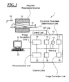
- FIG. 1 is a schematic representation of an MR system according to one exemplary embodiment of the invention
- FIG. 2 is a flowchart of the basic steps to correct distortions according to an exemplary embodiment of the invention.
- FIG. 3 is a flowchart of the basic steps to correct distortions according to a first variant of the method according to FIG. 2 .
- FIG. 4 is a flowchart of a possible method workflow to determine the relevant transformations or polynomial elements of the distortion correcting function in the implementation of a method according to FIG. 3 .
- FIG. 5 is a table with spherical harmonics for use in the method according to FIG. 4 .
- FIG. 6 is a graphical representation of correlation graphs for use in the method according to FIG. 4 .
- FIG. 7 is a flowchart of the basic steps to correct distortions according to a second variant of the method according to FIG. 2 .
- FIG. 8 is a flow diagram to explain a possible method to implement a hierarchical cluster search in the iterative determination of the correction parameters, for example in a method according to FIGS. 2 , 3 and 7 .
- a magnetic resonance system 1 is presented in a rough schematic in FIG. 1 . It includes the actual magnetic resonance scanner 10 with an examination space or patient tunnel into which an examination subject 12 on a bed 11 can be driven.
- the magnetic resonance scanner 10 is equipped in a typical manner with a basic field magnet system, a gradient coil system and a transmission and reception antenna system which, for example, includes a whole-body coil permanently installed in the magnetic resonance scanner 10 and possible additional local coils that can be variably arranged on the examination subject 12 .
- the MR system 1 furthermore has a central control unit 13 that is used to control the entire MR system 1 .
- the central control unit 13 has an image acquisition unit 14 for pulse sequence control. In this the sequence of RF pulses and gradient pulses is controlled depending on a selected imaging sequence.
- the central control unit 13 has an RF unit 15 to output the individual RF pulses and a gradient unit 16 to control the gradient coils, which RF unit 15 and gradient unit 16 communicate accordingly with the image acquisition unit 14 to emit the pulse sequences.
- the RF unit 15 includes not only a transmission part in order to emit the RF pulse sequences but also a reception part in order to acquire coordinated raw magnetic resonance data.
- a reconstruction unit 20 accepts the acquired raw data and reconstructs the MR images from these. How suitable raw data can be acquired via a radiation of RE pulses and the generation of gradient fields and how MR images can be reconstructed from these are known to those skilled in the art and need not be explained in detail here.
- Operation of the central control unit 13 can take place with an input unit 22 and a display unit 21 via which the entire MR system 1 can thus also be operated by an operator.
- MR images can also be displayed at the display unit 21 , and measurements can be planned and started by means of the input unit 22 , possibly in combination with the display unit 21 .
- diffusion gradients of different strengths are switched (shifted) during a measurement in addition to the gradients for the spatial coding.
- the principle of the acquisition of diffusion-weighted magnetic resonance images is also known to those skilled in the art and therefore does not need to be explained in detail.
- a displacement V(r,p) of the image information within the image plane occurs dominantly along the phase coding direction p, and in fact proportional to the amplitudes of the local interference field B(r,p) and inversely proportional to the pixel bandwidth BW along this direction, meaning that
- V ⁇ ( r , p ) B ⁇ ( r , p ) BW ( 1 )
- V(r,p) T+M ⁇ p+S ⁇ r.
- V can generally also be written as a polynomial distortion function as follows:
- a distorted image can be calculated back into an undistorted, corrected image with the function V.
- the coefficients a ij are thus the sought correction parameters.
- FIG. 2 schematically shows a possible method workflow for measurement and correction of diffusion images.
- an additional adjustment measurement R 2 is subsequently implemented and at least one additional reference image is acquired that corresponds to that of the first adjustment measurement, but with a different diffusion gradient activated, and the image is correspondingly distorted by the interference field of the developer gradient.
- the parameter a ij can then be determined, for example in an optimization method on the basis of the reference images generated in the adjustment measurements. It is iteratively sought to make the distorted image of the second adjustment measurement R 2 as similar as possible to the corresponding undistorted image of the first adjustment measurement R 1 by applying the transformation according to Equation (2b). This method naturally also functions when both reference images have been distorted differently by defined diffusion gradients, for example as in the aforementioned method according to Bodammer et al. A measure of similarity (also called a cost function) is used to assess the similarity. This means that the transformation is iteratively applied to the distorted image and it is sought to minimize the cost function or, respectively, to maximize the measure of similarity.
- Step 2 .III start values are established for the correction parameters, i.e. the start coefficients of the distortion correcting function.
- Step 2 .IV an image correction is then implemented with the distortion correcting function with the set start coefficients, wherein according to Equations (2a) and (2b) no alteration occurs in the readout direction r and a correction is only implemented in the phase coding direction p.
- Multiple sets of start coefficients are thereby typically started with, and for each start coefficient set a distortion map V(r,p) is calculated and applied to the image (i.e. to each individual value p).
- (n+1) start points are typically used in this method.
- (n+1) corrected images are then obtained.
- the number of start points is arbitrary.
- Step 2 .V the measure of similarity between the corrected image and the reference image is determined.
- the “Normalize Mutual Information” NMI can be applied as a typical measure of similarity.
- other measures of similarity can also be applied in principle.
- a check of whether the measure of similarity is sufficiently large (and thus whether the optimal correction parameters have been found) takes place in Step 2 .VI. If this is not the case, in Step 2 .VII new, optimized correction parameters are determined according to a predetermined strategy (that depends on the actual selected optimization method) and with these the loop with the method steps 2 .IV, 2 .V, 2 .VI and 2 .VII is run through again beginning with Step 2 .IV.
- Step 2 .IX the distorted diffusion images can subsequently be acquired and be respectively corrected in Step 2 .X using the predetermined correction function with the found, optimal correction parameters.
- the determination of the correction parameters can take place in a correction parameter determination unit 17 of the magnetic resonance system (see FIG. 1 ) of the central control unit 13 .
- the matching correction parameters can then be stored in a memory 19 by the correction parameter determination unit 17 or be transferred immediately to an image correction unit 18 that, using the distortion correcting function with the determined correction parameters, respectively corrected the magnetic resonance images reconstructed by the reconstruction unit 20 .
- the system-specific information is used in order to identify the polynomial elements in the non-linear polynomial transformation function according to Equation (4b) that lead to relevant image transformations under consideration of this system-specific information upon application of a diffusion gradient during the measurement, wherein the relevance of the image transformations is assessed with a predetermined relevancy criterion.
- relevant transformations or “relevant polynomial elements” that are selected are also used synonymously, even if naturally which polynomial elements lead to relevant transformations is checked and these polynomial elements are then selected for the distortion function.
- Step 3 .III This establishment of a non-linear polynomial distortion correcting function via selection of the relevant polynomial elements in the transformation function according to Equation (4b) takes place in Step 3 .III.
- Steps 3 .I and 3 .II of the method according to FIG. 3 can coincide with Steps 2 .I and 2 .II of the method according to FIG. 2
- Steps 3 .IV through 3 .XI can correspond to Steps 2 .III through 2 .X.
- 3 are (for example) set to 1 for all polynomial elements that are considered to be relevant and set equal to 0 for all polynomial elements that are not considered to be relevant. In this way a distortion correcting function is automatically used which contains only the relevant polynomial elements.
- the selection of the relevant transformations or, respectively, polynomial elements can take place completely or additionally on the basis of heuristic information. For example, it is found in measurements of longer duration with high gradient load that thermal effects can lead to a distortion of the basic field. In echoplanar imaging, this appears as an image shift along the phase coding direction. If the reference image was now acquired at a first amplitude of the basic field and the image to be corrected was acquired at a second amplitude, in any case a transformation term a 00 is to be taken into account in the distortion correction. Depending on the system type, thermal effects of higher order (for example first or second order) can also occur that can be taken into account in the same manner.
- higher order for example first or second order
- the geometry of the eddy current fields is namely a system property due to the design of the components (for example of the gradient coil) of the eddy current surfaces in the magnet as well as the individual manufacturing tolerances. For example, if a gradient pulse with a defined time curve and defined amplitude is applied to an axis of the gradient coil, a reproducible interference field results with a defined geometry and a defined temporal decay.
- the temporal decay of the interference fields can be ignored for the following considerations.
- the spatial geometry of the interference field merely depends on the gradient axis (x, y, z) that is used or, respectively, (given simultaneous pulses on multiple physical axes) on the linear combination that is used and shows no dependency on the time curve or the amplitude of the generated gradient pulse.
- the amplitudes of the gradient pulses and their time curve only have influence on the amplitude of the interference field, i.e. on its scaling.
- This realization can be utilized within the scope of the invention in order to measure and store the geometry of the interference fields of each gradient axis for every individual system in a tune-up step, for example in the installation of the system and/or within the framework of the regular maintenance. Corresponding measurement methods that are generally conducted on phantoms are known to those skilled in the art and therefore need not be explained further herein.
- This tune-up step is shown as Step 4 .I in FIG. 4 .
- the measured geometric information can likewise be stored in a memory 19 of the system 1 (see FIG. 1 ) that can then be queried as needed by the correction parameter determination unit 17 in order to implement additional calculations with said information.
- the field geometries are normally expressed in the form of spherical harmonics, for example for the gradient axis in the x-direction in the form
- B x ⁇ ( r , ⁇ , ⁇ ) ⁇ ⁇ A x ⁇ ( n , m ) ⁇ Norm ⁇ ( n , m ) ⁇ ( r / r 0 ) n ⁇ cos ⁇ ( m ⁇ ⁇ ⁇ ) ⁇ P n m ⁇ ( cos ⁇ ( ⁇ ) ) + ⁇ ⁇ B x ⁇ ( n , m ) ⁇ Norm ⁇ ( n , m ) ⁇ ( r / r 0 ) n ⁇ sin ⁇ ( m ⁇ ⁇ ) ⁇ P n m ⁇ ( cos ⁇ ( ⁇ ) ) ( 5 ) with a suitable normalization (for example what is known as the L-Norm 4 ):
- Equation (7) The spherical harmonics A nm and B nm that are specified in Equation (7) are indicated in the table in FIG. 5 up to the third order for the polar coordinates r, ⁇ , ⁇ on the one hand (left column) and for the Cartesian coordinates of the system x, y, z on the other hand (right column).
- the field geometry in the x-direction can thus be completely mathematically described up to the third order in that the coefficients A x (0,0) . . . B x (3,3) are simply specified.
- the field geometries B y (r, ⁇ , ⁇ ) and B z (r, ⁇ , ⁇ ) in the y-direction and in the z-direction can be described in the same way.
- a tune-up step 4 . 1 for each x-, y-, z-coordinate the geometry of the interference field generated by the respective gradient can consequently be specified precisely in polar coordinates r, ⁇ , ⁇ according to Equation (7) and then be converted into (for example) x-, y-, z-coordinates in a form B x (x, y, z), B y (x ,y, z) and B z (x, y, z).
- b x , b y , b z are the relative amplitudes of the diffusion gradients (i.e. the amplitude values relative to one another or, respectively, relative to a standard value).
- Steps 4 .II through 4 .VII The additional steps for this are presented in FIG. 4 in Steps 4 .II through 4 .VII. These steps must be respectively re-implemented for each measurement of the current determination of the correction parameters, which is different than for the method step 4 .I.
- method step 4 .II the relative association of the amplitudes b x , b y , b z of the diffusion gradients with the individual gradient axes is thereby initially determined.
- a determination of the position (i.e. the bearing and orientation) of the current slice then takes place in method step 4 .III for the imaging within the x-, y-, z-coordinate system.
- Step 4 .IV the transformation matrix T between physical and logical coordinates and the center of symmetry of the transformation must therefore then be determined for the current slice. This can take place in the following manner:
- this matrix contains the conversion factors for the conversion from pixel positions to millimeter values and vice versa.
- the vector (x 0 , y 0 , z 0 ) describes the center of the current slice.
- the coordinate s in the direction of the slice perpendiculars is always zero in this convention.
- Equation (11) If the coordinates x, y, z from Equation (11) are inserted into the right column of the spherical harmonic according to the table in FIG. 5 , the spherical polynomials A 00 . . . B 33 are obtained for the coordinates r, p, s so that via insertion into Equation (7) the geometry of the interference fields B z (r,p,s), B y (r,p,s), B z (r,p,s) for the individual gradient axes x, y, z in the imaging coordinates r, p, s are obtained.
- the interference field B(r,p) that is determined in this way essentially corresponds to the sought function V(r,p) so that the relative coefficients for the transformations in the image plane can also be determined by sorting the individual components of the function B(r,p) according to the polynomials in r,p.
- these are not the absolute coefficients a ij that must still be determined later within the scope of the correction method, but rather are only the relative values in relation to one another.
- Step 4 .V This transformation of the spatial geometry of the field interferences for the diffusion measurement into the logical imaging coordinates takes place in Step 4 .V of the method workflow shown in FIG. 4 .
- the magnitude of the corresponding pixel shift in the image relative to the pixel shifts caused by the other polynomial elements can then be considered on the basis of the previously acquired information about the interference field geometry (Step VI), and those polynomial elements that actually lead to relevant transformations or to the “most relevant” transformations can thus be selected in Step 4 .VII.
- a calculation of the respective pixel shift at selected points of the image plane in magnetic resonance images corresponding to one another can be identified from the current adjustment measurements that are implemented for the respective usable measurement. For example, a set of test image pixels or, respectively, test points (r i , p i ) can thereby be established (possibly also with a weighting W i ) that describes the region of interest (ROI) in the image.
- W i region of interest
- test image pixels at which the shift is calculated are distributed isotropically in the slice on a circle with radius FOV/2.
- the number of points is determined from the highest order n of the field interferences to be corrected. Since the number of field extremes amounts at most to 2 n , at least (2 n +1) points on the circle must be used for the calculation of the pixel shift in order to avoid undersampling.
- the sum of the absolute magnitudes of the pixel shift V ij (r,p) is then determined and, for example, those transformations with the greatest values can be classified as a relevance criterion.
- a fixed number of transformations can be predetermined, for example the five transformations with the greatest contributions. This means that only five polynomial elements are definitively accounted for within the polynomial distortion function.
- a limit value can also be established as a relevancy criterion, for example. For example, all transformations that lead to a pixel shift of more than two pixels in the center can be taken into account. Combinations of the most varied relevancy criteria are likewise also possible.
- a number of transformations can also always be taken into account in a targeted manner, for example the affine transformations. Moreover, a specific number (for example two) of additional relevant transformations is then permitted according to the previously cited criteria. Furthermore, a number of transformations can also be specifically excluded, for example because the associated correction parameters or polynomial coefficients prove to be unstable in the registration.
- the relevance of the transformation is advantageously determined depending on the image content.
- the region of the image that contains the significant information can be determined initially via application of an intensity threshold.
- This image region can also have an irregular shape.
- a rectangle comprising the relevant region can advantageously be established as a “bounding box”. The transformations that have the greatest effect in this image region or at test image pixels selected within this image region are then classified as relevant and used.
- the processing speed is markedly increased and at the same time the precision of the similarity comparison is improved.
- the first point is due to the reduction of the image section that is to be considered; the last point is due to the exclusion of large noise regions.
- the calculation of the cost function should reasonably be limited only to the relevant region; the entire original image then remains for the image transformation. If the image were also limited to the relevant image section for the transformation, portions of the image could slide out of the overlap region with the reference image and other portions could slide in due to the transformation. Possible unwanted jumps [discontinuities] in the cost function could thereby arise.
- the use of two transformations that correlate strongly with one another can be avoided given the assessment of the relevance.
- the strength of the per pair correlations can initially be determined.
- One possibility for correlation determination is based on the heuristic analysis of the spatial transformation properties. For example, p and p 3 exhibit similar transformation geometries. Correlations can be determined more precisely via a statistical analysis. Therefore, according to a first hierarchy step the determined n-sets of “more optimal” transformation parameters are considered. For example, for each set the determined coefficients of the p-transformation are then depicted versus the determined coefficients of the p 3 transformation in an a 09 /a 03 diagram. If the transformations are strongly correlated, the data points are arranged along a line. For example, this case can be identified by calculating a correlation coefficient. Such a case is shown above in FIG. 6 . Here a clear arrangement of the data points appears along a line.
- a “more expensive” measure of similarity can be used.
- Such a more expensive measure of similarity can be achieved via more “binnings” in the MRI or via an oversampling of the image information, whereby the precision increases such that the strength of the correlation is sufficiently reduced.
- What is understood by a “binning” is the number of sub-divisions of a histogram.
- the effect of the decorrelation by using a more expensive measure of similarity is shown below in FIG. 6 .
- one of the two strongly correlated transformations can be excluded. For example, the transformation with the smaller contribution, or that with the greater complexity (i.e. the higher order), can be excluded.
- the relevant transformations or, respectively, the associated, relevant polynomial elements depend on the position and the orientation of the respective image plane. Different transformations can thus be relevant to different slices of an image stack, and the distortion correcting function can also accordingly look different. Moreover, the selection of the relevant transformations also depends on the diffusion direction.
- the geometry of the interference field generated from the respective gradient according to Equation (7) can be precisely specified mathematically up to the third order, and therefore the spatial interference field that is generated as a whole can be described according to Equation (12) in r,p imaging coordinates for a concrete measurement with known, normalized diffusion direction.
- Equation (12) Given application of spherical function of higher order, terms of a correspondingly higher order can naturally also be taken into account. A reasonable upper limit of the order results from the resolution of the measurement method used in the tune-up step.
- the interference field can also be described absolutely in good approximation with a global scaling factor a H corresponding to Equation (12)
- the description of the interference field B(r,p) according to Equation (14) can also be drawn upon directly to correct the distorted images, wherein the scaling factor a H would be to be determined as a correction parameter.
- the eddy currents of 0th and 1st order are actively compensated in modern systems, it is reasonable to handle these separately and to set up a distortion function V(r,p) as follows:
- the coefficients a 00 , a 11 , a 01 for the affine transformations and additionally the scaling factor a H are thus sought as correction parameters, for example in an optimization method. It is thereby to be heeded that the individual interference fields B k (r,p) do not need to be identical with those in Equation (14); rather, the terms of 0th and 1st order can be removed here since these terms are handled separately.
- the scaling factor a H is accordingly also different than in Equation (14).
- FIG. 7 shows a flow chart for a corresponding correction method. Steps 7 .I and 7 .II of this method coincide with the steps 2 .I and 2 .II of the method according to FIG. 2 .
- Step 7 .III a relative association of the amplitude d k of the diffusion gradients with the gradient axes occurs, for example (1, 1, 0).
- Step 7 .IV the relative interference field geometry B k (r, ⁇ , ⁇ ) is then defined in spherical coordinates or B k (x, y, z) in the Cartesian coordinate system of the system for each gradient axis k.
- Step 7 .V start values are defined for the coefficients or, respectively, correction parameters a 00 , a 10 , a 01 , a H .
- An image correction with the distortion correcting function according to Equation (15) subsequently takes place in Step 7 .VI with the used start coefficients, analogous to Steps 2 .IV in FIG. 2 or 3 .V in FIG. 3 .
- Steps 7 .VII through 7 .XII can again corresponding to Steps 2 .V through 2 .X.
- Step 8 .II a set of start parameters for the optimization is then established for each of these cluster elements.
- a reasonable order of magnitude of the individual parameters should be used, i.e. that a maximum shift of two pixels within the relevant image region takes place for every individual transformation, for example.
- the cluster elements differ sufficiently from one another, meaning that the associated started parameters differ homogeneously in a multidimensional parameter space.
- the selected optimization method is then run independently, and in fact with an “advantageous” similarity function (for example with an NMI with low number of binnings) to shorten the processing time.
- an “advantageous” similarity function for example with an NMI with low number of binnings
- a separate set of “more optimal” correction parameters is then determined for each of these optimizations.
- these S sets of “more optimal” correction parameters are then subject to a grouping analysis.
- the mutual separations (intervals) of the “optimal” correction parameters are thereby determined in multidimensional space and one or more groups with similar, “optimal” correction parameters is determined on this basis.
- step 8 the cluster element is with the greatest similarity to the reference image is determined for each group. All other cluster elements are discarded.
- Step 8 VI the number of previously determined groups is then set as a new number S of cluster elements.
- Step 8 .VII it is checked whether the new number S of cluster elements is equal to 1. If this is not the case, an optimization is implemented again for the new cluster elements and the method steps 8 .III through 8 .VII are run through again. This second stage can then operate with a “more expensive” but thus more precise similarity function until finally it is established in Step 8 .VIII that the current number S of cluster elements or groups amounts only to 1. The method can then be ended in Step 8 .VIII.
- the method described here can also be used advantageously within the framework of the method described in DE 10 2009 003 889 for improvement of the correction of image distortions. At least one of the two adjustment measurements is thereby respectively implemented with a predetermined diffusion weighting in three orthogonal diffusion directions and correction parameters for the three orthogonal diffusion directions are determined based on this. Correction parameters for diffusion-weighted MR images with arbitrary diffusion direction can then be determined via linear combination from the correction parameters for the three orthogonal diffusion directions.
- both the methods from Bodammer et al, and those from Haselgrove et al. can be used.
- the first adjustment measurement with the first diffusion weighting corresponds to the reference measurement without diffusion gradient. In this case this means that the first diffusion weighting would be zero.
- the second adjustment measurement can then be implemented with the predetermined diffusion weighting in the three orthogonal diffusion directions, for example. Given application of the method according to the invention to the method from Bodammer et al., the first adjustment measurement with the first diffusion weighting would be the negative diffusion weighting, for example, while the second adjustment measurement would be the measurement with the same positive diffusion weighting.
Landscapes
- Physics & Mathematics (AREA)
- High Energy & Nuclear Physics (AREA)
- Condensed Matter Physics & Semiconductors (AREA)
- General Physics & Mathematics (AREA)
- Health & Medical Sciences (AREA)
- Nuclear Medicine, Radiotherapy & Molecular Imaging (AREA)
- General Health & Medical Sciences (AREA)
- Radiology & Medical Imaging (AREA)
- Engineering & Computer Science (AREA)
- Signal Processing (AREA)
- Vascular Medicine (AREA)
- Magnetic Resonance Imaging Apparatus (AREA)
Abstract
Description
r′=r (2a)
p′=p+V(r,p) (2b)
V(r,p)=a 00 +a 10 r+a 01 p+a 11 rp+a 20 r 2 +a 02 p 2 (4a)
or third order:
V(r,p)=a 00 a 10 r+a 01 p+a 11 rp+a 20 r 2 +a 02 p 2 a 21 rp 2 +a 12 r 2 p+a 30 r 3 a 03 p 3 (4b)
with a suitable normalization (for example what is known as the L-Norm 4):
B x(r,φ,θ)=ΣΣA x(n,m)A nm +ΣΣB x(n,m)B nm (7)
B(x,y,z)=b xBx(x,y,z)+b y B y(x,y,z)+b z B z(x,y,z) (8)
wherein R represents the matrix of the direction cosines between the axes of the two coordinate systems, Res is the diagonal matrix with the resolution information (i.e. this matrix contains the conversion factors for the conversion from pixel positions to millimeter values and vice versa. The vector (x0, y0, z0) describes the center of the current slice. The coordinate s in the direction of the slice perpendiculars is always zero in this convention. The center of symmetry of the interference fields in the normal case lies at the isocenter of the magnet, i.e. given (x, y, z)=(0, 0, 0) or, respectively, (p, r, s)=(p0,r0, s0). In order to keep the different transformations as independent from one another as possible, it suggests itself to describe all transformations relative to this defined zero point in the acquired slice. In total the coordinate transformation can thus be represented as:
x=T 11(p−p0)+T 12(r−r0)+T 13(s−s0)
y=T 21(p−p0)+T 22(r−r0)+T 23(s−s0)
z=T 31(p−p0)+T 32(r−r0)+T 33(s−s0) (11)
B(r,p)=c x B x(r,p)+c y B y(r,p)+c z B z(r,p) (12)
(r 1 ,p 1)=(−FOVr/2, −FOVp/2)
(r 2 ,p 2)=(−FOVr/2, +FOVp/2)
(r 3 ,p 3)=(+FOVr/2, −FOVp/2)
(r 4 ,p 4)=(−FOVr/2, +FOVp/2) (13)
wherein FOVr and FOVp specify the image field (field of view) in the readout direction r and in the phase coding direction p.
wherein ck/aH=dk is set in the last step. According to Equation (1), B(r,p) can be equated with the sought distortion function V(r,p) except for the given factor BW.
Claims (15)
Applications Claiming Priority (3)
| Application Number | Priority Date | Filing Date | Title |
|---|---|---|---|
| DE102010001577 | 2010-02-04 | ||
| DE102010001577A DE102010001577B4 (en) | 2010-02-04 | 2010-02-04 | Method for reducing distortions in diffusion imaging and magnetic resonance system |
| DE102010001577.6 | 2010-02-04 |
Publications (2)
| Publication Number | Publication Date |
|---|---|
| US20110187367A1 US20110187367A1 (en) | 2011-08-04 |
| US8508226B2 true US8508226B2 (en) | 2013-08-13 |
Family
ID=44341047
Family Applications (1)
| Application Number | Title | Priority Date | Filing Date |
|---|---|---|---|
| US13/020,302 Active 2031-12-03 US8508226B2 (en) | 2010-02-04 | 2011-02-03 | Method and magnetic resonance system to reduce distortions in diffusion imaging |
Country Status (3)
| Country | Link |
|---|---|
| US (1) | US8508226B2 (en) |
| CN (1) | CN102144923B (en) |
| DE (1) | DE102010001577B4 (en) |
Cited By (5)
| Publication number | Priority date | Publication date | Assignee | Title |
|---|---|---|---|---|
| US20110304334A1 (en) * | 2010-06-10 | 2011-12-15 | Thorsten Feiweier | Magnetic resonance method and apparatus to correct image distortions in diffusion-weighted imaging |
| US20150316635A1 (en) * | 2012-12-12 | 2015-11-05 | Koninklijke Philips N.V. | Motion detection and correction method for magnetic resonance diffusion weighted imaging (dwi) |
| US11061096B2 (en) | 2016-11-09 | 2021-07-13 | Cr Development Ab | Method of performing diffusion weighted magnetic resonance measurements on a sample |
| US11215683B2 (en) | 2017-05-17 | 2022-01-04 | Siemens Healthcare Gmbh | Method and magnetic resonance apparatus correction of multiple distortion effects during magnetic resonance imaging |
| US11327138B2 (en) | 2019-09-30 | 2022-05-10 | Siemens Healthcare Gmbh | Method for compensating eddy currents when creating measurement data by means of magnetic resonance |
Families Citing this family (21)
| Publication number | Priority date | Publication date | Assignee | Title |
|---|---|---|---|---|
| WO2008128088A1 (en) | 2007-04-13 | 2008-10-23 | The Regents Of The University Of Michigan | Systems and methods for tissue imaging |
| JP2011512963A (en) * | 2008-02-29 | 2011-04-28 | ザ リージェンツ オブ ザ ユニバーシティ オブ ミシガン | System and method for imaging changes in tissue |
| JP5619448B2 (en) * | 2009-08-20 | 2014-11-05 | 株式会社東芝 | Magnetic resonance imaging system |
| DE102010013605B4 (en) | 2010-03-31 | 2013-03-14 | Siemens Aktiengesellschaft | Reduction of distortions in MR diffusion imaging |
| DE102010035539B4 (en) | 2010-08-26 | 2012-04-05 | Siemens Aktiengesellschaft | Method for compensating eddy current fields in magnetic resonance imaging and magnetic resonance apparatus |
| DE102010041125B4 (en) | 2010-09-21 | 2015-07-30 | Siemens Aktiengesellschaft | Spatial correction of image data from a series of magnetic resonance images |
| DE102010041587B4 (en) * | 2010-09-29 | 2012-10-31 | Siemens Aktiengesellschaft | Suppression and / or elimination of spurious signals in magnetic resonance imaging with an ultrashort echo time imaging sequence |
| US9773311B2 (en) | 2011-06-29 | 2017-09-26 | The Regents Of The University Of Michigan | Tissue phasic classification mapping system and method |
| DE102011082266B4 (en) * | 2011-09-07 | 2015-08-27 | Siemens Aktiengesellschaft | Imaging a partial area at the edge of the field of view of an examination object in a magnetic resonance system |
| WO2013078370A1 (en) | 2011-11-23 | 2013-05-30 | The Regents Of The University Of Michigan | Voxel-based approach for disease detection and evolution |
| US9851426B2 (en) * | 2012-05-04 | 2017-12-26 | The Regents Of The University Of Michigan | Error analysis and correction of MRI ADC measurements for gradient nonlinearity |
| DE102013224406B4 (en) | 2013-11-28 | 2015-10-08 | Siemens Aktiengesellschaft | Correction of Distortions in Magnetic Resonance Diffusion Images |
| DE102014201944B4 (en) | 2014-02-04 | 2015-11-12 | Siemens Aktiengesellschaft | RF pulse adjustment method and RF pulse adjustment device |
| US10102681B2 (en) * | 2015-07-29 | 2018-10-16 | Synaptive Medical (Barbados) Inc. | Method, system and apparatus for adjusting image data to compensate for modality-induced distortion |
| US10466381B2 (en) * | 2015-12-28 | 2019-11-05 | Baker Hughes, A Ge Company, Llc | NMR logging in formation with micro-porosity by using first echoes from multiple measurements |
| US10650512B2 (en) | 2016-06-14 | 2020-05-12 | The Regents Of The University Of Michigan | Systems and methods for topographical characterization of medical image data |
| US10545211B2 (en) * | 2017-06-28 | 2020-01-28 | Synaptive Medical (Barbados) Inc. | Method of correcting gradient nonuniformity in gradient motion sensitive imaging applications |
| EP3699624A1 (en) * | 2019-02-25 | 2020-08-26 | Koninklijke Philips N.V. | Calculation of a b0 image using multiple diffusion weighted mr images |
| DE102020200786A1 (en) | 2020-01-23 | 2021-07-29 | Siemens Healthcare Gmbh | Correction of distorted diffusion-weighted magnetic resonance image data |
| DE102022202093A1 (en) | 2022-03-01 | 2023-09-07 | Siemens Healthcare Gmbh | Process for the optimized recording of diffusion-weighted measurement data of an examination object using a magnetic resonance system |
| CN114675221A (en) * | 2022-03-15 | 2022-06-28 | 武汉联影生命科学仪器有限公司 | Magnetic resonance gradient correction compensation factor determination method, correction method and device |
Citations (8)
| Publication number | Priority date | Publication date | Assignee | Title |
|---|---|---|---|---|
| US6288540B1 (en) * | 1999-05-21 | 2001-09-11 | University Of Rochester | Optimized orthogonal gradient technique for fast quantitative diffusion MRI on a clinical scanner |
| US6642716B1 (en) * | 2002-05-15 | 2003-11-04 | Koninklijke Philips Electronics, N.V. | Diffusion tensor magnetic resonance imaging including fiber rendering using hyperstreamlines |
| US20070223832A1 (en) | 2006-03-23 | 2007-09-27 | Kazuhiko Matsumoto | Diffusion weighted image processing apparatus and recording medium for recording image analysis program |
| US20100171498A1 (en) | 2009-01-02 | 2010-07-08 | Karin Auslender | Magnetic resonance method and apparatus to reduce distortions in diffusion imaging |
| US20110052031A1 (en) | 2009-09-02 | 2011-03-03 | Thorsten Feiweier | Method and magnetic resonance system to correct distortions in image data |
| US20110085722A1 (en) | 2009-10-14 | 2011-04-14 | Thorsten Feiweier | Correction of distortions in diffusion-weighted magnetic resonance imaging |
| US20110241679A1 (en) * | 2010-03-31 | 2011-10-06 | Thorsten Feiweier | Magnetic resonance method and apparatus to reduce distortions in diffusion images |
| US20130033262A1 (en) * | 2011-08-02 | 2013-02-07 | David Andrew Porter | Method to generate magnetic resonance exposures |
Family Cites Families (2)
| Publication number | Priority date | Publication date | Assignee | Title |
|---|---|---|---|---|
| JP4812420B2 (en) * | 2005-12-12 | 2011-11-09 | 株式会社東芝 | Magnetic resonance imaging apparatus and image correction evaluation method |
| CN101470179B (en) * | 2007-12-29 | 2012-06-27 | 西门子(中国)有限公司 | Method and apparatus for distortion calibration in magnetic resonance imaging |
-
2010
- 2010-02-04 DE DE102010001577A patent/DE102010001577B4/en active Active
-
2011
- 2011-01-21 CN CN201110023622.2A patent/CN102144923B/en active Active
- 2011-02-03 US US13/020,302 patent/US8508226B2/en active Active
Patent Citations (8)
| Publication number | Priority date | Publication date | Assignee | Title |
|---|---|---|---|---|
| US6288540B1 (en) * | 1999-05-21 | 2001-09-11 | University Of Rochester | Optimized orthogonal gradient technique for fast quantitative diffusion MRI on a clinical scanner |
| US6642716B1 (en) * | 2002-05-15 | 2003-11-04 | Koninklijke Philips Electronics, N.V. | Diffusion tensor magnetic resonance imaging including fiber rendering using hyperstreamlines |
| US20070223832A1 (en) | 2006-03-23 | 2007-09-27 | Kazuhiko Matsumoto | Diffusion weighted image processing apparatus and recording medium for recording image analysis program |
| US20100171498A1 (en) | 2009-01-02 | 2010-07-08 | Karin Auslender | Magnetic resonance method and apparatus to reduce distortions in diffusion imaging |
| US20110052031A1 (en) | 2009-09-02 | 2011-03-03 | Thorsten Feiweier | Method and magnetic resonance system to correct distortions in image data |
| US20110085722A1 (en) | 2009-10-14 | 2011-04-14 | Thorsten Feiweier | Correction of distortions in diffusion-weighted magnetic resonance imaging |
| US20110241679A1 (en) * | 2010-03-31 | 2011-10-06 | Thorsten Feiweier | Magnetic resonance method and apparatus to reduce distortions in diffusion images |
| US20130033262A1 (en) * | 2011-08-02 | 2013-02-07 | David Andrew Porter | Method to generate magnetic resonance exposures |
Non-Patent Citations (6)
| Title |
|---|
| "Comprehensive Approach for Correction of Motion and Distortion in Diffusion-Weighted MRI," Rohde et al., Magnetic Resonance in Medicine, vol. 51 (2004) pp. 103-114. |
| "Correction for Distortion of Echo-Planar Images Used to Calculate the Apparent Diffusion Coefficient," Haselgrove et al., Magnetic Resonance in Medicine, vol. 36 (1996) pp. 960-964. |
| "Correction of Eddy-Current Distortions in Diffusion Tensor Images Using the Known Directions and Strengths of Diffusion Gradients," Zhuang, et al., Journal of Magnetic Resonance Imaging, vol. 24 (2006) pp. 1188-1199. |
| "Eddy Current Correction in Diffusion-Weighted Imaging Using Pairs of Images Acquired With Opposite Diffusion Gradient Polarity," Bodammer et al., Magnetic Resonance in Medicine, vol. 51 (2004) pp. 188-193. |
| "Mutual Information," Latham et al., Scholarpedia (2008). |
| U.S. Appl. No. 13/020,302, filed Feb. 4, 2011. |
Cited By (9)
| Publication number | Priority date | Publication date | Assignee | Title |
|---|---|---|---|---|
| US20110304334A1 (en) * | 2010-06-10 | 2011-12-15 | Thorsten Feiweier | Magnetic resonance method and apparatus to correct image distortions in diffusion-weighted imaging |
| US8928319B2 (en) * | 2010-06-10 | 2015-01-06 | Siemens Aktiengesellschaft | Magnetic resonance method and apparatus to correct image distortions in diffusion-weighted imaging |
| US20150316635A1 (en) * | 2012-12-12 | 2015-11-05 | Koninklijke Philips N.V. | Motion detection and correction method for magnetic resonance diffusion weighted imaging (dwi) |
| US10241182B2 (en) * | 2012-12-12 | 2019-03-26 | Koninklijke Philips N.V. | Motion detection and correction method for magnetic resonance diffusion weighted imaging (DWI) |
| US11061096B2 (en) | 2016-11-09 | 2021-07-13 | Cr Development Ab | Method of performing diffusion weighted magnetic resonance measurements on a sample |
| USRE49978E1 (en) | 2016-11-09 | 2024-05-21 | The Brigham And Women's Hospital, Inc. | Method of performing diffusion weighted magnetic resonance measurements on a sample |
| US11215683B2 (en) | 2017-05-17 | 2022-01-04 | Siemens Healthcare Gmbh | Method and magnetic resonance apparatus correction of multiple distortion effects during magnetic resonance imaging |
| US11327138B2 (en) | 2019-09-30 | 2022-05-10 | Siemens Healthcare Gmbh | Method for compensating eddy currents when creating measurement data by means of magnetic resonance |
| DE102019215046B4 (en) | 2019-09-30 | 2023-09-21 | Siemens Healthcare Gmbh | Method for compensating for eddy currents when recording measurement data using magnetic resonance |
Also Published As
| Publication number | Publication date |
|---|---|
| DE102010001577A1 (en) | 2011-09-22 |
| CN102144923B (en) | 2014-12-17 |
| CN102144923A (en) | 2011-08-10 |
| DE102010001577B4 (en) | 2012-03-08 |
| US20110187367A1 (en) | 2011-08-04 |
Similar Documents
| Publication | Publication Date | Title |
|---|---|---|
| US8508226B2 (en) | Method and magnetic resonance system to reduce distortions in diffusion imaging | |
| US8487617B2 (en) | Magnetic resonance method and apparatus to reduce distortions in diffusion images | |
| CN103238082B (en) | MR imaging using a multi-point Dixon technique and low resolution calibration | |
| US8548217B2 (en) | Method and magnetic resonance system to correct distortions in image data | |
| JP5525596B2 (en) | Accelerated B1 mapping | |
| JP5485663B2 (en) | System and method for automatic scan planning using symmetry detection and image registration | |
| JP5138043B2 (en) | Magnetic resonance imaging system | |
| US9651644B2 (en) | Method and magnetic resonance system to acquire MR data in a predetermined volume segment of an examination subject | |
| KR20150131124A (en) | Signal inhomogeneity correction and performance evaluation apparatus | |
| JP2016504144A (en) | Metal resistant MR imaging | |
| Chung et al. | An improved PSF mapping method for EPI distortion correction in human brain at ultra high field (7T) | |
| US20200209333A1 (en) | Magnetic resonance imaging apparatus and medical complex image processing apparatus | |
| US6586935B1 (en) | Magnetic resonance image artifact correction using navigator echo information | |
| JP2006255046A (en) | Magnetic resonance imaging method and image processing apparatus | |
| US8659295B2 (en) | Method and device for magnetic resonance imaging | |
| US20160124065A1 (en) | Method and apparatus for correction of magnetic resonance image recordings with the use of a converted field map | |
| JP2020531140A (en) | Data-driven correction of phase-dependent artifacts in magnetic resonance imaging systems | |
| US10775469B2 (en) | Magnetic resonance imaging apparatus and method | |
| JP5618683B2 (en) | Magnetic resonance imaging apparatus and brightness non-uniformity correction method | |
| JP6202761B2 (en) | Magnetic resonance imaging apparatus and processing method thereof | |
| US10036793B2 (en) | Method and apparatus for reconstructing magnetic resonance images with phase noise-dependent selection of raw data | |
| US7812603B2 (en) | Method for determining local deviations of a main magnetic field of a magnetic resonance device | |
| US9880249B2 (en) | Method for determining distortion-reduced magnetic resonance data and magnetic resonance system | |
| EP4053580A1 (en) | System and method for acquisition of a magnetic resonance image as well as device for determining a trajectory for acquisition of a magnetic resonance image | |
| US12013451B2 (en) | Noise adaptive data consistency in deep learning image reconstruction via norm ball projection |
Legal Events
| Date | Code | Title | Description |
|---|---|---|---|
| AS | Assignment |
Owner name: SIEMENS AKTIENGESELLSCHAFT, GERMANY Free format text: ASSIGNMENT OF ASSIGNORS INTEREST;ASSIGNORS:FEIWEIER, THORSTEN;HUWER, STEFAN;PORTER, DAVID ANDREW;AND OTHERS;SIGNING DATES FROM 20110207 TO 20110208;REEL/FRAME:026134/0126 |
|
| STCF | Information on status: patent grant |
Free format text: PATENTED CASE |
|
| AS | Assignment |
Owner name: SIEMENS HEALTHCARE GMBH, GERMANY Free format text: ASSIGNMENT OF ASSIGNORS INTEREST;ASSIGNOR:SIEMENS AKTIENGESELLSCHAFT;REEL/FRAME:039271/0561 Effective date: 20160610 |
|
| FPAY | Fee payment |
Year of fee payment: 4 |
|
| MAFP | Maintenance fee payment |
Free format text: PAYMENT OF MAINTENANCE FEE, 8TH YEAR, LARGE ENTITY (ORIGINAL EVENT CODE: M1552); ENTITY STATUS OF PATENT OWNER: LARGE ENTITY Year of fee payment: 8 |
|
| AS | Assignment |
Owner name: SIEMENS HEALTHINEERS AG, GERMANY Free format text: ASSIGNMENT OF ASSIGNORS INTEREST;ASSIGNOR:SIEMENS HEALTHCARE GMBH;REEL/FRAME:066088/0256 Effective date: 20231219 |