US8339897B2 - Automatic dispersion extraction of multiple time overlapped acoustic signals - Google Patents
Automatic dispersion extraction of multiple time overlapped acoustic signals Download PDFInfo
- Publication number
- US8339897B2 US8339897B2 US12/644,862 US64486209A US8339897B2 US 8339897 B2 US8339897 B2 US 8339897B2 US 64486209 A US64486209 A US 64486209A US 8339897 B2 US8339897 B2 US 8339897B2
- Authority
- US
- United States
- Prior art keywords
- slowness
- dispersion
- estimates
- time
- phase
- Prior art date
- Legal status (The legal status is an assumption and is not a legal conclusion. Google has not performed a legal analysis and makes no representation as to the accuracy of the status listed.)
- Active, expires
Links
- 239000006185 dispersion Substances 0.000 title claims abstract description 99
- 238000000605 extraction Methods 0.000 title abstract description 32
- 238000012545 processing Methods 0.000 claims description 39
- 238000009826 distribution Methods 0.000 claims description 19
- 238000007596 consolidation process Methods 0.000 claims description 5
- 230000004807 localization Effects 0.000 claims description 4
- 238000007670 refining Methods 0.000 claims description 2
- 238000004422 calculation algorithm Methods 0.000 abstract description 14
- 230000002452 interceptive effect Effects 0.000 abstract description 3
- 238000000034 method Methods 0.000 description 27
- 238000001228 spectrum Methods 0.000 description 16
- 239000013598 vector Substances 0.000 description 13
- 238000001276 Kolmogorov–Smirnov test Methods 0.000 description 11
- 238000013459 approach Methods 0.000 description 11
- 238000012360 testing method Methods 0.000 description 11
- 239000011159 matrix material Substances 0.000 description 10
- 238000005457 optimization Methods 0.000 description 9
- 230000008569 process Effects 0.000 description 9
- 230000004044 response Effects 0.000 description 6
- 239000011435 rock Substances 0.000 description 6
- 238000003491 array Methods 0.000 description 5
- 238000010586 diagram Methods 0.000 description 5
- 238000004458 analytical method Methods 0.000 description 4
- 230000008859 change Effects 0.000 description 4
- 230000001902 propagating effect Effects 0.000 description 4
- 238000007476 Maximum Likelihood Methods 0.000 description 2
- 239000000654 additive Substances 0.000 description 2
- 230000000996 additive effect Effects 0.000 description 2
- 230000008901 benefit Effects 0.000 description 2
- 238000012512 characterization method Methods 0.000 description 2
- 238000004590 computer program Methods 0.000 description 2
- 230000001186 cumulative effect Effects 0.000 description 2
- 238000005315 distribution function Methods 0.000 description 2
- 239000012530 fluid Substances 0.000 description 2
- 238000003064 k means clustering Methods 0.000 description 2
- 230000000644 propagated effect Effects 0.000 description 2
- 238000013139 quantization Methods 0.000 description 2
- 238000005070 sampling Methods 0.000 description 2
- 241000143437 Aciculosporium take Species 0.000 description 1
- 101100243399 Caenorhabditis elegans pept-2 gene Proteins 0.000 description 1
- 235000019687 Lamb Nutrition 0.000 description 1
- VPNMENGBDCZKOE-LNYNQXPHSA-N [(1R,5S)-8-methyl-8-azabicyclo[3.2.1]octan-3-yl] 3-hydroxy-2-phenylpropanoate [(1S,2S,4R,5R)-9-methyl-3-oxa-9-azatricyclo[3.3.1.02,4]nonan-7-yl] (2S)-3-hydroxy-2-phenylpropanoate (1R,3S)-1,2,2-trimethylcyclopentane-1,3-dicarboxylic acid Chemical compound CC1(C)[C@H](CC[C@@]1(C)C(O)=O)C(O)=O.CC1(C)[C@H](CC[C@@]1(C)C(O)=O)C(O)=O.CN1[C@H]2CC[C@@H]1CC(C2)OC(=O)C(CO)c1ccccc1.CN1[C@H]2CC(C[C@@H]1[C@H]1O[C@@H]21)OC(=O)[C@H](CO)c1ccccc1 VPNMENGBDCZKOE-LNYNQXPHSA-N 0.000 description 1
- 238000007621 cluster analysis Methods 0.000 description 1
- 238000004891 communication Methods 0.000 description 1
- 238000012937 correction Methods 0.000 description 1
- 230000001419 dependent effect Effects 0.000 description 1
- 230000001066 destructive effect Effects 0.000 description 1
- 230000010339 dilation Effects 0.000 description 1
- 238000002224 dissection Methods 0.000 description 1
- 230000000694 effects Effects 0.000 description 1
- 230000007613 environmental effect Effects 0.000 description 1
- 238000011156 evaluation Methods 0.000 description 1
- 230000005284 excitation Effects 0.000 description 1
- 238000001914 filtration Methods 0.000 description 1
- 239000004615 ingredient Substances 0.000 description 1
- 239000000463 material Substances 0.000 description 1
- 238000005259 measurement Methods 0.000 description 1
- 238000012986 modification Methods 0.000 description 1
- 230000004048 modification Effects 0.000 description 1
- 238000007781 pre-processing Methods 0.000 description 1
- 229910052704 radon Inorganic materials 0.000 description 1
- SYUHGPGVQRZVTB-UHFFFAOYSA-N radon atom Chemical compound [Rn] SYUHGPGVQRZVTB-UHFFFAOYSA-N 0.000 description 1
- 238000011160 research Methods 0.000 description 1
- 238000004088 simulation Methods 0.000 description 1
- 238000013519 translation Methods 0.000 description 1
- 238000010200 validation analysis Methods 0.000 description 1
Images


Classifications
-
- G—PHYSICS
- G01—MEASURING; TESTING
- G01V—GEOPHYSICS; GRAVITATIONAL MEASUREMENTS; DETECTING MASSES OR OBJECTS; TAGS
- G01V1/00—Seismology; Seismic or acoustic prospecting or detecting
- G01V1/40—Seismology; Seismic or acoustic prospecting or detecting specially adapted for well-logging
- G01V1/44—Seismology; Seismic or acoustic prospecting or detecting specially adapted for well-logging using generators and receivers in the same well
- G01V1/48—Processing data
- G01V1/50—Analysing data
-
- G—PHYSICS
- G01—MEASURING; TESTING
- G01V—GEOPHYSICS; GRAVITATIONAL MEASUREMENTS; DETECTING MASSES OR OBJECTS; TAGS
- G01V1/00—Seismology; Seismic or acoustic prospecting or detecting
- G01V1/28—Processing seismic data, e.g. for interpretation or for event detection
- G01V1/30—Analysis
-
- G—PHYSICS
- G01—MEASURING; TESTING
- G01V—GEOPHYSICS; GRAVITATIONAL MEASUREMENTS; DETECTING MASSES OR OBJECTS; TAGS
- G01V1/00—Seismology; Seismic or acoustic prospecting or detecting
- G01V1/28—Processing seismic data, e.g. for interpretation or for event detection
- G01V1/30—Analysis
- G01V1/307—Analysis for determining seismic attributes, e.g. amplitude, instantaneous phase or frequency, reflection strength or polarity
-
- G—PHYSICS
- G01—MEASURING; TESTING
- G01V—GEOPHYSICS; GRAVITATIONAL MEASUREMENTS; DETECTING MASSES OR OBJECTS; TAGS
- G01V2210/00—Details of seismic processing or analysis
Definitions
- This invention relates broadly to the extraction of the slowness dispersion characteristics of multiple possibly interfering signals in broadband acoustic waves, and more particularly to the processing of acoustic waveforms where there is dispersion, i.e. a dependence of wave speed and attenuation with frequency.
- Dispersive processing of borehole acoustic data has been a key ingredient for the characterization and estimation of rock properties using borehole acoustic modes.
- the most common parameters describing the dispersion characteristics are the wavenumber, k(f), and the attenuation, A(f), both functions of the frequency f and are of great interest in characterization of rock and fluid properties around the borehole.
- they are of interest in a variety of other applications such as non-destructive evaluation of materials using ultrasonic waves or for handling ground roll in surface seismic applications, where the received data exhibits dispersion that needs to be estimated.
- the dispersion characteristic consisting of the phase and group slowness (reciprocal of velocity) are linked to the wavenumber k as follows:
- s g s ⁇ + f ⁇ d s ⁇ d f
- One class of extraction methods uses physical models relating the rock properties around the borehole to the predicted dispersion curves. Waveform data collected by an array of sensors is back propagated according to each of these modeled dispersion curves and the model is adjusted until there is good semblance (defined below) among these back propagated waveforms indicating a good fit of the model to the data.
- An example is the commercial DSTC algorithm used for extracting rock shear velocity from the dipole flexural mode (see C. Kimball, “Shear slowness measurement by dispersive processing of borehole flexural mode,” Geophysics , vol. 63, no. 2, pp. 337-344, March 1998) (in this case we directly invert for the rock property of interest).
- a high resolution method appropriate for shorter arrays was developed using narrow band array processing techniques applied to frequency domain data obtained by performing an FFT on the array waveform data (see S. Lang, A. Kurkjian, J. McClellan, C. Morris, and T. Parks, “Estimating slowness dispersion from arrays of sonic logging waveforms,” Geophysics , vol. 52, no. 4, pp. 530-544, April 1987 and M. P. Ekstrom, “Dispersion estimation from borehole acoustic arrays using a modified matrix pencil algorithm,” ser. 29th Asilomar Conference on Signals, Systems and Computers, vol. 2, 1995, pp. 449-453).
- Slowness dispersion characteristics of multiple possibly interfering signals in broadband acoustic waves as received by an array of two or more sensors are extracted without using a physical model.
- the problem of dispersion extraction is mapped to the problem of reconstructing signals having a sparse representation in an appropriately chosen over-complete dictionary of basis elements.
- a sparsity penalized signal reconstruction algorithm can be used where the sparsity constraints are implemented by imposing a l 1 norm type penalty.
- the candidate modes that are extracted can be consolidated by means of a clustering algorithm to extract phase and group slowness estimates at a number of frequencies which are then used to reconstruct the desired dispersion curves. These estimates can be further refined by building time domain propagators when signals are known to be time compact, such as by using the continuous wavelet transform.
- the result is a general approach (without using specific physical models) for estimating dispersion curves for multiple signals (unknown number) that could overlap in the time-frequency domain.
- the algorithm advantageously involves the solution of a convex optimization problem that is computationally efficient to implement.
- Another advantage of this approach is that the model order selection is automatically taken care of as the sparsity conditions ensure that only the candidate modes are extracted as long as the regularization parameter for the penalty is chosen in an appropriate range.
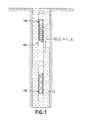
- FIG. 1 is a schematic representation of a physical set-up for acquisition of waves in a borehole.
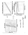
- FIG. 2 illustrates the array waveforms and modal dispersion curves governing the propagation of the acoustic energy.
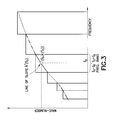
- FIG. 3 is a schematic representation of the piecewise linear approximation to the dispersion curve. Also shown are the dispersion parameters corresponding to a first order Taylor series approximation in a band around f 0 .
- FIG. 4 illustrates the efficacy of local Taylor expansions of orders one and two in capturing the behavior of a typical quadrupole dispersion curve.
- FIG. 5 illustrates a collection of broadband basis in a given band around the center frequency f 0 .
- FIG. 6 is a schematic representation of the column sparsity of the signal support in ⁇ . Sparsity of the number of modes in the band (a) implies a column sparsity in mode representation in the broadband basis in the band (b).
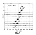
- FIG. 7 illustrates noisy data in a band containing two time overlapping modes.
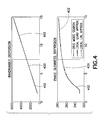
- FIG. 8 illustrates an example of the behavior of the residual as a function of ⁇ . Note how the mode leakage occurs into the residual as we increase ⁇ .
- the KS test is used to detect changes in the distribution of the residuals as a function of ⁇ .
- FIG. 9 illustrates an example of the KS test statistic sequence and the p-value sequence for determining the operating ⁇ .
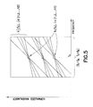
- FIG. 10 is a schematic representation of the discretization of the parameter space of phase and group slowness in a band and the mismatch of the dictionary with respect to the true modes in the data.
- FIG. 11 illustrates an example of the mode clusters in the phase and group slowness domain due to dictionary mismatch corresponding to the 6 largest peaks in the modulus image.
- FIG. 12 illustrates the flow of processing in a band for dispersion extraction in the f-k domain.
- FIG. 13 is a schematic representation of the first order Taylor series approximation to the dispersion curve in a band around the center frequency fa of the mother wavelet at scale a.
- FIG. 14 illustrates a combination of the space-time and frequency-wavenumber processing for dispersion extraction using CWT (depicting the (a) f-k domain and (b) time domain characteristics of the CWT coefficients in terms of the propagation parameters at a given scale).
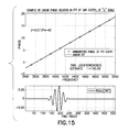
- FIG. 15 illustrates an example of implication of time compactness of the CWT coefficients at a given scale at one sensor on the phase of the FFT coefficients in the band.
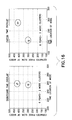
- FIG. 16 illustrates an example of mode consolidation and model order selection using the phase slowness and time location estimates.
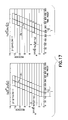
- FIG. 17 illustrates the broadband space time propagators in the CWT domain.
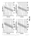
- FIG. 18 illustrates the reconstructed CWT coefficients at a given scale for two mode dispersion extraction problem with significant time overlap.
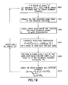
- FIG. 19 illustrates the flow of the processing in the space time domain processing the output of the broadband processing in the f-k domain as applied to the CWT coefficients at a given scale.
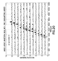
- FIG. 20 illustrates an array waveform data with two time overlapping modes.
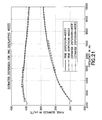
- FIG. 21 illustrates extracted dispersion curves in frequency bands.
- the solid lines denote the true underlying dispersion curves for the two modes.
- the extracted curves are shown by solid lines marked with circles.
- Individual embodiments may be described as a process which is depicted as a flowchart, a flow diagram, a data flow diagram, a structure diagram, or a block diagram. Although a flowchart may describe the operations as a sequential process, many of the operations can be performed in parallel or concurrently. In addition, the order of the operations may be re-arranged. A process may be terminated when its operations are completed, but could have additional steps not discussed or included in a figure. Furthermore, not all operations in any particularly described process may occur in all embodiments. A process may correspond to a method, a function, a procedure, a subroutine, a subprogram, etc. When a process corresponds to a function, its termination corresponds to a return of the function to the calling function or the main function.
- Embodiments of the invention may be implemented, at least in part, either manually or automatically.
- Manual or automatic implementations may be executed, or at least assisted, through the use of machines, hardware, software, firmware, middleware, microcode, hardware description languages, or any combination thereof.
- the program code or code segments to perform the necessary tasks may be stored in a machine readable medium.
- a processor(s) may perform the necessary tasks.
- an acoustic source ( 100 ) which may be in communication with surface equipment is fired in a fluid filled borehole and the resulting waves that are generated in the borehole are recorded at a linear array of sonic sensors (hydrophones) ( 102 ) located on the acoustic tool.
- the relationship between the received waveforms and the wavenumber-frequency (k-f) response of the borehole to the source excitation is captured via the following equation (2),
- s ⁇ ( l , t ) ⁇ 0 ⁇ ⁇ ⁇ 0 ⁇ ⁇ S ⁇ ( f ) ⁇ Q ⁇ ( k , f ) ⁇ e i ⁇ ⁇ 2 ⁇ ⁇ ⁇ ⁇ ⁇ f ⁇ ⁇ t ⁇ e - i ⁇ ⁇ kz l ⁇ d f ⁇ d k
- the wavenumber as a function of frequency i.e. the function(s) k m (f)
- the wavenumber as a function of frequency i.e. the function(s) k m (f)
- ⁇ f ⁇ [f 0 ⁇ f B ,f 0 +f B ] (7)
- FIG. 4 illustrates the results of approximating a typical dispersion curve (quadrupole) with first and second order Taylor expansions (shown by the green ( 400 ) and red ( 402 ) curves, respectively).
- the local fit obtained thereby is quite adequate for capturing the local behavior of the dispersion curve.
- Those skilled in the art will note the efficacy of local Taylor expansions of orders one and two in capturing the behavior of a typical quadrupole dispersion curve.
- the local linear and quadratic approximations shown in red and blue respectively overlay and match the true dispersion curve well in a local interval. In other words, one can approximate the dispersion curve as composed of piecewise linear segments over adjacent frequency bands.
- the dispersion curve is parameterized by the phase and the group slowness.
- a corresponding step ( 1202 ) is shown in FIG. 12 .
- it is assumed that it is constant over the frequency band of interest, i.e., a m (f) ⁇ a m (f 0 ), ⁇ f ⁇ F
- FIG. 3 is a schematic depiction of the local linear approximation to a dispersion curve over adjacent frequency bands.
- a framework for dispersion extraction in f-k domain in a band can be understood by first considering a broadband basis element P F (k(f 0 ),k′(f 0 )) (also called a broadband propagator) in a band F corresponding to a given phase slowness
- ⁇ ⁇ ( f ) [ e - i2 ⁇ ⁇ ⁇ ( k ⁇ ( f 0 ) + k ′ ⁇ ( f 0 ) ⁇ ( f - f 0 ) ) ⁇ z 1 e - i2 ⁇ ⁇ ⁇ ( k ⁇ ( f 0 ) + k ′ ⁇ ( f 0 ) ⁇ ( f - f 0 ) ) ⁇ z 2 ⁇ e - i2 ⁇ ⁇ ⁇ ( k ⁇ ( f 0 ) + k ′ ⁇ ( f 0 ) ⁇ ( f - f 0 ) ) ⁇ z L ] ⁇ C L ⁇ 1 ( 14 )
- FIG. 5 illustrates an over-complete basis of broadband propagators in the given band in the f-k domain.
- a matrix X corresponding to x is constructed by reshaping it like so:
- the sparsity structure of the signal support in the broadband basis described above is also known as a simultaneous sparse structure in the literature e.g., see J. A. Tropp, A. C. Gilbert, and M. J. Strauss (J. A. Tropp, A. C. Gilbert, and M. J. Strauss, “Algorithms for simultaneous sparse approximation. part ii: Convex relaxation,” Signal Processing, special issue on Sparse approximations in signal and image processing , vol. 86, pp. 572-588, April 2006). It is well known that for this set-up the optimal processing consists of solving the following optimization problem:
- OPT 0 ⁇ ⁇ arg ⁇ min X ⁇ ⁇ Y - ⁇ ⁇ ⁇ x ⁇ 2 + ⁇ ⁇ ⁇ j ⁇ ⁇ 1 X C ⁇ ( j ) ( 18 )
- OPT 1 ⁇ ⁇ arg ⁇ min X ⁇ ⁇ Y - ⁇ ⁇ ⁇ x ⁇ 2 + ⁇ 1 ⁇ ⁇ X ⁇ 2 ( 19 )
- the first issue is selection of regularization parameter ⁇ in the optimization problem OPT 1 .
- this parameter governs the sparsity of the solution and thus is critical for model order selection.
- this parameter In the relaxed setup of OPT 1 , apart from governing the sparsity of the solution this parameter also affects the spectrum estimates. This is due to solution shrinkage resulting from the l 1 , part of the 1 l 2 penalty.
- the second issue is the assumption that the true modes lie in the over-complete dictionary used above is not generally true. This has consequences for model order selection as well as for the estimates of dispersion parameters. However, if the true modes are close to elements in the dictionary, the effects are small and can be readily handled.
- tests are used between the distribution of residuals to select the regularization parameter ⁇ in the optimization problem OPT 1 .
- the first role is that of general regularization of the solution where due to ill-conditioning of the matrix ⁇ the noise can get amplified.
- the second role is that of model order selection, which is essentially related to selection of the sparsest (and correct) basis for signal representation. In the context of finding sparse solutions these two aspects go hand in hand. Note, for example, that at a very low value of ⁇ , the solution to OP T1 comes close to the Least Squares (LS) solution.
- LS Least Squares
- the observations described above support a strategy for selecting the regularization parameter by varying ⁇ over a range and detecting changes in distribution of the residuals and selecting an operating ⁇ that mitigates noise and minimizes the signal leakage into the residual while still finding the right signal subspace.
- a corresponding step ( 1208 ) is shown in FIG. 12 .
- the Kolmogorov-Smirnov (KS) test W. Feller, “On the Kolmogorov-Smirnov limit theorems for empirical distributions,” Annals of Mathematical Statistics , vol. 19, p. 177, 1948
- the intersection point of the test curves qualitatively signifies the tradeoff between over-fitting and under-fitting of the data.
- the rate of change of distribution of the residual is more rapid due to mode leakage into the residual.
- the solutions for this range of ⁇ exhibit stability in terms of getting to the right signal support.
- the KS tests can be performed between residuals either in the frequency domain or in the time domain. If the modes are time compact, as is often the case, it is useful to compare the distributions of the residuals in the space-time domain.
- FIG. 9 An example of the KS test-curves for distribution of residuals in time domain and the corresponding operating range of ⁇ is shown in FIG. 9 . It is also possible to develop a similar test for changes in the distribution of the signal support of X as a means to select a suitable value for the regularization parameter.
- FIG. 10 A schematic depiction of the dictionary mismatch with respect to the true modal dispersion is shown in FIG. 10 .
- S F the true signal in band F as given by equation 12
- ⁇ F be the best and unique l 2 approximation to S F in the constructed over-complete dictionary ⁇ .
- the illustrated approach in the f-k domain has been shown to be robust to presence of time overlapped modes.
- this approach makes no use of time information and in particular this makes the group slowness estimates sensitive to noise and interference. Therefore, in order to make use of time compactness of the modes the broadband dispersion extraction method in the f-k domain is combined with the EPRT type broadband dispersion extraction in the space-time domain.
- the CWT of the array data is used in order to retain the time information in this context. Initially, the dispersion parameters in the CWT domain are identified. Recall here (a more detailed exposition can be found, for example, see A. Grossmann, R. Kronland-Martinet, J. Morlet.
- the broadband dispersion extraction methodology in the f-k domain described in the previous section can be extended in a straightforward manner to the CWT coefficients.
- a joint method for dispersion extraction in the CWT domain that utilizes the broadband multiple mode extraction methodology in the f-k domain and the time compactness of modes in the space-time domain in a manner similar to the EPRT algorithm is used.
- the difference is that while constructing the broadband propagators as in equation 13, a reference location z 0 at the centroid of the sensor array is chosen, i.e., replace the z i by z i ⁇ z 0 in equation 13. This is done to facilitate the time processing as it decouples the errors in the group slowness estimated from the time location estimate obtained below.
- a corresponding step ( 1900 ) is shown in FIG. 19 .
- This f-k domain processing is followed by a model order selection and a mode consolidation step ( 1902 , FIG. 19 ) which is modified to include estimates of time location.
- the model order selection is now done based on clustering in the phase slowness and time location domain. The reason for this is that time location estimates obtained from the broadband processing in f-k domain are more robust than the group slowness estimates.
- time compactness of the modes implies a linear phase relationship across frequency in the mode spectrum is exploited to obtain the time location estimates. Based on the linear phase relationship one can obtain estimates of the time location of the modes at scale a from estimates of the mode spectrum at the reference sensor by fitting a straight line through the unwrapped phase of the estimated mode spectrum in the band. The slope of this line is related to the index of the time location estimate of the mode via the relationship
- a space-time processing refines the mode amplitude spectrum and group slowness estimates.
- the CWT coefficients for a mode are related across the sensor array by a time shift corresponding to the group slowness and a phase correction given by the difference of the group and phase slowness. Consequently, broadband propagators in the space-time domain each of which is defined as a time compact window propagating at the group slowness with a complex phase change across sensors in proportion to the difference of the phase and group slowness can be considered.
- u T (t) denote a rectangular window function of width T centered at zero. Then the broadband space time propagator at a scale a can be written as—
- p ⁇ 1 , ... ⁇ , p ⁇ M arg ⁇ min p 1 , ... ⁇ , p M ⁇ ⁇ Y a - U a ⁇ ( p ) ⁇ C ⁇ a ⁇ ( p ) ⁇ ( 38 )
- p ⁇ 1 , ... ⁇ , p ⁇ M arg ⁇ min p 1 , ... ⁇ , p M ⁇ ⁇ Y a - U a ⁇ ( p ) ⁇ C ⁇ a ⁇ ( p ) ⁇ ( 39 )
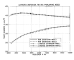
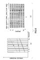
- FIG. 20 shows the array of received waveforms comprising two time overlapping modes and added noise.
- the SNR is set to be 0 dB in the sense of total signal to total noise energy.
- the exponential model is given a perturbation by incorporating sensor gain and phase errors to make the simulation more realistic.
- FIG. 21 shows the result of applying the described approach in both the f-k and space-time domains in four frequency bands.
- the solid lines represent the true dispersion curves and the curves marked by circles are the dispersion curves extracted by estimating the phase and group slownesses in these bands. The match of the estimate to the true curves validates the described approach.
- features of the invention may be implemented in computer programs stored on a computer readable medium and run by processors, application specific integrated circuits and other hardware.
- the computer programs and hardware may be distributed across devices including but not limited to tooling which is inserted into the borehole and equipment which is located at the surface, whether onsite or elsewhere.
Landscapes
- Physics & Mathematics (AREA)
- Life Sciences & Earth Sciences (AREA)
- Engineering & Computer Science (AREA)
- Remote Sensing (AREA)
- Acoustics & Sound (AREA)
- Environmental & Geological Engineering (AREA)
- Geology (AREA)
- General Life Sciences & Earth Sciences (AREA)
- General Physics & Mathematics (AREA)
- Geophysics (AREA)
- Measurement Of Velocity Or Position Using Acoustic Or Ultrasonic Waves (AREA)
Abstract
Description
-
- where the group slowness sg and phase slowness sφ are not independent; in fact, they satisfy
-
- There is therefore the need to extract these quantities of interest from the measured acoustic data.
-
- for l=1, 2, . . . , L and where s(l,t) denotes the pressure at time t at the l-th sensor located at a distance zl from the source; S(f) is the source spectrum and Q(k,f) is the wavenumber-frequency response of the borehole. Typically the data is acquired in the presence of noise (environmental noise and sensor noise) and interference (unmodelled energy), collectively denoted by w(l,t). The noisy observations at the set of sensors can be expressed as,
y(l,t)=s(l,t)+w(l,t) (3) - It has been shown that the complex integral in the wavenumber (k) domain in
equation 2 can be approximated by contribution due to the residues of a finite number, M(f) of poles of the system response, (3). Specifically,
- for l=1, 2, . . . , L and where s(l,t) denotes the pressure at time t at the l-th sensor located at a distance zl from the source; S(f) is the source spectrum and Q(k,f) is the wavenumber-frequency response of the borehole. Typically the data is acquired in the presence of noise (environmental noise and sensor noise) and interference (unmodelled energy), collectively denoted by w(l,t). The noisy observations at the set of sensors can be expressed as,
-
- where km(f) and am(f) are the wavenumber and the attenuation as functions of frequency. Consequently,
-
- where Sm(f)=S(f)qm(f). Under this signal model, the data acquired at each frequency across the sensors can be expressed as shown in
FIG. 2 , wherein the array waveforms and modal dispersion curves govern the propagation of the acoustic energy. The task is therefore to estimate these dispersion curves given the received waveforms.
- where Sm(f)=S(f)qm(f). Under this signal model, the data acquired at each frequency across the sensors can be expressed as shown in
-
- In other words the data at each frequency is a superposition of M exponentials sampled with respect to the sensor locations z1, . . . , zL. The above system of equations corresponds to a sum of exponential model at each frequency. M(f) is the effective number of exponentials at frequency f. A corresponding method step (1200) is shown in
FIG. 12 .
- In other words the data at each frequency is a superposition of M exponentials sampled with respect to the sensor locations z1, . . . , zL. The above system of equations corresponds to a sum of exponential model at each frequency. M(f) is the effective number of exponentials at frequency f. A corresponding method step (1200) is shown in
k m(f)≈k m(f 0)+k′ m(f 0)(f−f 0),∀fε
-
- It is apparent that over the set of frequencies fεF, the collection of sampled exponentials (for a fixed m) {vm(f)}fεℑ as defined above corresponds to a line segment in the f-k domain thereby parametrizing the wavenumber response of the mode in the band in terms of phase and group slowness. In the following the band F is represented by F which is a finite set of frequencies contained in F.
F={f 1 ,f 2 , . . . ,f Nf }⊂:f 0 εF (9)
- Essentially in a time sampled system the discrete set of frequencies in F correspond to the discrete set of frequencies in the DFT of the data y(l,t) of
equation 3. Under the linear approximation of dispersion curves in the band F, a broadband system of equations in the band can be expressed as,
- It is apparent that over the set of frequencies fεF, the collection of sampled exponentials (for a fixed m) {vm(f)}fεℑ as defined above corresponds to a line segment in the f-k domain thereby parametrizing the wavenumber response of the mode in the band in terms of phase and group slowness. In the following the band F is represented by F which is a finite set of frequencies contained in F.
-
- where S(f)=[S1(f), S2(f) . . . SM(f)]T is the vector of mode(s) spectrum at f and VM(f)=[v1(f1), v2(f1) . . . vM(f1)]. In other words, the data in a frequency band is a superposition of exponentials at each frequency where the parameters of the complex exponentials are linked by phase and group slowness and attenuation factor across the frequencies. Accordingly,
-
- The matrix PF(m) corresponds to the matrix of exponentials for the wavenumber response for mode m in the band F, and the vector SF(m) is the vector of the mode spectrum for mode m in the band F. The signal (without noise) in band F is a superposition of M modes and can be written as,
-
- Now note that, under the piecewise linear approximation of the dispersion curves over adjacent frequency bands (could be partially overlapping), the problem of dispersion extraction can be reduced to the problem of estimating the linear parameters of these curves in each band. These are the corresponding phase and group slowness and attenuation and yield the dispersion curve in the band. The entire dispersion curve can then be obtained by combining the dispersion curves estimated as above in each of these bands. Thus, without loss of generality, it is reasonable to ignore the attenuation as this is usually small and does not bias the estimation of the wavenumber, and focus on dispersion extraction in a band. This can however be incorporated in the basis elements as shown above, but with the penalty of generating a much larger and computationally expensive system to solve. Alternatively, these could be estimated in a subsequent step after the wavenumbers have been estimated. So, given the data Y in the frequency band F it is desirable to estimate the model order M, the dispersion curves of the modes as modeled by the wavenumber response PF(m) in the band F, and the mode spectrum SF(m) for all m=1, 2, . . . , M.
and group slowness k′(f0) as an operator.
-
- consisting of exponential vectors φ(f) given by
-
- From equation 12 (and ignoring the attenuation) it can be appreciated that the data in a given band is a superposition of broadband basis elements. Under this set-up a methodology for dispersion extraction in a band includes the following steps:
- Given the band F around a center frequency f0, form an over-complete dictionary of broadband basis elements PF(kij(f0),k′ij(f0), ij=1, . . . , N in the f-k domain spanning a range of group and phase slowness. The number of basis elements, N, in the dictionary is much larger than the column span of all the elements in the dictionary. A corresponding step (1204) is shown in
FIG. 12 . - Assuming that the broadband signal is in the span of the broadband basis elements from the over-complete dictionary, the presence of a few significant modes in the band implies that the signal representation in the over-complete dictionary is sparse. In other words, the signal is composed of a superposition of few broadband propagators in the over-complete dictionary.
- The problem of slowness dispersion extraction in the band can then be mapped to that of finding the sparsest signal representation in the over-complete dictionary of broadband propagators.
- Given the band F around a center frequency f0, form an over-complete dictionary of broadband basis elements PF(kij(f0),k′ij(f0), ij=1, . . . , N in the f-k domain spanning a range of group and phase slowness. The number of basis elements, N, in the dictionary is much larger than the column span of all the elements in the dictionary. A corresponding step (1204) is shown in
- Therefore, the problem of dispersion estimation is mapped to that of finding the sparsest signal representation in an over-complete dictionary of broadband propagators spanning a range of group and phase slowness. Note that while, in general, the true propagators might not lie in the chosen over complete basis, this approach will still work so long as there are dictionary elements close to the true ones. In that case, the nearest basis elements are chosen in the sparse representation, possibly more than one for each mode, and the mismatch is subsumed in the noise.
- From equation 12 (and ignoring the attenuation) it can be appreciated that the data in a given band is a superposition of broadband basis elements. Under this set-up a methodology for dispersion extraction in a band includes the following steps:
In line with the broadband system given by
-
- where Ψn(F)=PF(ki(f0),k′j(f0)) of equation 13 with n=i+(j−1)N2, i=1, 2, . . . , N1, j=1, 2, . . . , N2 and N=N1×N2 is the number of elements in the over-complete dictionary.
S F =Φx M (16)
-
- with a special coefficient vector xMεN.N×1 f which has the property that most of its elements equal 0, i.e., it is sparse, with the only non-zero elements being the ones that correspond to the locations of the M propagators of

equation 12. Note that as the above equation is massively under-determined, many coefficient vectors would satisfy it; however only the special vector has the type of sparsity stated above.
- with a special coefficient vector xMε
-
- Note that each column in XM corresponds to a basis element in Φ and therefore only those M columns in it corresponding to the location of the propagators representing the signal modes have non-zero entries, which are in fact simply the SF(m), m=1, . . . , M. With M<<N, XM exhibits column sparsity as shown in
FIG. 6 . The column support of X is represented by 1x C, the column indicator function of X, consisting of 1's at the locations of the columns containing non-zero entries and 0's elsewhere. Assuming that the broadband propagators corresponding to the signal modes are linearly independent, among all coefficientvectors satisfying equation 16, XM has the smallest column support which corresponds to that of the true modes, i.e., the signal support. The signal support corresponds to the slowness dispersion parameters of the modes present in the data and its cardinality is the model order in the band.
- Note that each column in XM corresponds to a basis element in Φ and therefore only those M columns in it corresponding to the location of the propagators representing the signal modes have non-zero entries, which are in fact simply the SF(m), m=1, . . . , M. With M<<N, XM exhibits column sparsity as shown in
Y=Φx+W,xε
-
- with respect to an over-complete basis ΦεM.N×N.N.N f12f of broadband propagators, estimate X having the greatest column sparsity. Its column support would then yield the estimated dispersion parameters and model order in the band. The problem of dispersion extraction is thus mapped to that of finding the sparsest (column sparse) signal representation in an over-complete dictionary of broadband basis propagators in the given band. As will be described below, a convex optimization algorithm for dispersion extraction that exploits the particular sparsity structure of the signal support may be utilized.
- with respect to an over-complete basis Φε
-
- for some appropriately chosen value of λ for the penalty term which counts the number of non-zero columns of X. The latter is also known as 0l2 norm penalty and imposing it in the f-k domain on the solution dictates sparsity in the number of modes with a non-sparse spectrum in the frequency band. Note that when the additive noise W is i.i.d. Gaussian, solving this optimization problem is equivalent to solving a Maximum-Likelihood (ML) estimation problem. However, imposing the 0l2 penalty poses a combinatorial problem, which in general is very difficult to solve. It was proposed in J. A. Tropp, A. C. Gilbert, and M. J. Strauss to relax the 0l2 norm penalty to the 1l2 norm penalty (defined below) which is the closest convex relaxation to it. In accordance with one embodiment of this invention the following convex relaxation is used to solve the sparse reconstruction problem:
-
- for some appropriately chosen value of λ and where the norm 1∥X∥2, is its 1l2 norm defined as the sum of the l2 norms of the columns of the X
-
- where X(:,j) is the jth column of X. A corresponding step (1206) is shown in
FIG. 12 .
- where X(:,j) is the jth column of X. A corresponding step (1206) is shown in
-
- Then the KS test statistic for CDF(r) with respect to a reference distribution CDFref(r) is given by the supremum of the difference of the cumulative distribution functions:
-
- The properties of the KS test statistic D, its limiting distribution and the asymptotic properties can be found in (W. Feller, “On the Kolmogorov-Smirnov limit theorems for empirical distributions,” Annals of Mathematical Statistics, vol. 19, p. 177, 1948). Essentially the KS statistic is a measure of similarity between two distributions. In order to apply the KS-test the steps shown in TABLE A are performed.
-
STEP 1. Pick an increasing sequence of the regularization parameter Λ=λ1<λ2< . . . <λn. In practice it is sufficient to choose this sequence as Λ=logspace (a0, a1, n), a0, a1εR. This choice implies λ1=10a0 and λn=10a1. -
STEP 2. Find the sequence of solutions {circumflex over (x)}λ, λεΛ and sequence of residual vectors Rλ=Y−Φ{circumflex over (x)}λ. Denote the empirical distribution of residuals w.r.t. the solution Xλ by CDFλ(r) where r denotes the variable for residual. -
STEP 3. Conduct KS tests between the residuals—- 3a. Choose two reference distributions, viz., CDF1(r) corresponding to the minimum value λ1 of regularization parameter and CDFn(r) corresponding to the maximum value λn of the regularization parameter.
- 3b. Find the sequence of KS-test statistics Di,n=supr|CDFn(r)−CDFi(r)|, i=1, 2, . . . , n and the corresponding p-value sequence Pi,n. Similarly find the sequence of KS-test statistics Di,1=supr|CDF1(r)−CDFi(r)|, i=1, 2, . . . , n and the corresponding p-value sequence Pi,1.
-
STEP 4. Plot the sequences Di,n and Di,1 as a function of λi. The operating say λ* is then taken as the point of intersection of these two curves. A similar operating point can also be obtained by choosing the intersection point of the p-value sequences Pi,n and P1,i.
∥Ŝ F(N ε)−S F∥≦ε, (23)
-
- i.e. under appropriate quantization, the signal can be well represented in the over-complete basis. This mismatch can then be modeled as an additive error,
-
- where now the coefficient vector x {circumflex over (x)}εN.N×1 f corresponds to the representation for the approximate signal ŜF. Thus, in the presence of dictionary mismatch the problem of dispersion extraction maps to that of finding the dispersion parameters of the best approximation to the signal in the over-complete basis of broadband propagators. Sparsity in the number of modes in SF still translates to sparsity in the representation of the approximation ŜF in the over-complete basis Φ and the sparse reconstruction algorithm OPT1 is still employed for dispersion extraction. However, this affects the model order selection and dispersion estimates. In order to understand this in the current context, consider the modulus image, MI, in the dispersion parameter space:
MI(x)(i,j)=∥X(:,i+j·(N 1−1))∥2 (25) - whose (i,j)th element comprises the l2 norm of the column of X (reshaped matrix of x) corresponding to the ith value of the phase slowness and jth value of the group slowness. Note that the support of the modulus image corresponds to the broadband signal support and the corresponding dispersion parameters can be read from the image. A corresponding step (1210) is shown in
FIG. 12 . Now the result of the dictionary mismatch with respect to the true dispersion parameters of the modes is a clustered set of peaks in the modulus image described above. This clustered set of points corresponds to the set of phase and group slowness points that are closest to the true phase and group slowness points. This is due to approximate signal representation of the true signal in the over-complete basis, obtained in the solution to the optimization problem OPT1. The mode clusters can also be formed if there is a high level of coherence between the broadband basis elements. An example of such clustering around the true values of phase and group slowness is shown inFIG. 11 .
- where now the coefficient vector x {circumflex over (x)}ε
-
-
STEP 1. Pick a certain number of peaks say Np corresponding to the largest values in ModIM(X). -
STEP 2. Perform a k-means clustering of the peak points in the phase and the group slowness domain. -
STEP 3. Declare the resulting number of clusters as the model order. -
STEP 4. Mode consolidation—- 4a. The mode spectrum corresponding to each cluster is obtained by summing up the estimated coefficients corresponding to the points in the cluster.
- 4b. The corresponding dispersion estimates are taken to be the average over the dispersion parameters corresponding to the cluster points.
-
The CWT C(a,b) of signal s(t) at scale (dilation factor) a and shift (translation) b is given by
-
- where G(f) is the Fourier transform of the analyzing (mother) wavelet g(t) and S(f) is the Fourier transform of the signal being analyzed. The analyzing mother wavelet g(t) is chosen to satisfy some admissibility condition. For the sake of exposition first consider a single mode. Then under the complex exponential model of equation 5 (and ignoring attenuation), the CWT coefficients at scale a and time shift b of the received waveform at sensor l, is given by,
-
- Assuming that a first order Taylor series approximation holds true in the effective bandwidth of the analyzing wavelet around the center frequency fa of the analyzing wavelet, see
FIG. 13 , the CWT coefficients at scale a obey the following relationship,
- Assuming that a first order Taylor series approximation holds true in the effective bandwidth of the analyzing wavelet around the center frequency fa of the analyzing wavelet, see
-
- where δl,F=zl−zl′ denotes the inter-sensor spacing between sensor l and l′ and where
-
- is a compensating phase factor. Thus, for a given mode the CWT coefficients of the mode at a given scale undergo a shift according to the group slowness across the sensors with a complex phase change proportional to the difference of the phase and the group slowness. These ideas are depicted in
FIG. 14( b). Moreover, take the Fourier transform with respect to the time shift b and obtain a simple exponential relationship
C l(a,f)=e i2πδl.l′ (k(fa )+k′(fa )(f−fa )) C l(a,f) (30) - for all fεa the effective frequency support of the analyzing wavelet at scale a. Thus the same exponential relationship holds for the CWT coefficients in the frequency domain as for the original signal mode with the frequency band now given by the support at scale a of the analyzing wavelet.
- is a compensating phase factor. Thus, for a given mode the CWT coefficients of the mode at a given scale undergo a shift according to the group slowness across the sensors with a complex phase change proportional to the difference of the phase and the group slowness. These ideas are depicted in
-
- The following observations can be made regarding the CWT transform of the modes at a given scale:
- Time compactness of mode m implies time compactness of the CWT coefficients Cl m(a,b) at each scale. The time-frequency support of the modes in the CWT domain obeys the time-frequency uncertainty relation corresponding to the mother wavelet used—at higher frequencies (smaller scales) the time resolution is sharp but the frequency resolution is poor and vice-versa.
- Time compactness in turn implies a linear phase relationship across frequencies fεa in the coefficients of the mode spectrum Cl m(a,f) of the CWT data Cl m(a,b) at any sensor l and whereis the effective bandwidth of the analyzing wavelet at scale a.

- Equations 30 and 31 indicate that the same exponential relationship holds for the CWT coefficients at each scale a in the frequency domain as for the original signal with the frequency band now given by the support at that scale of the analyzing wavelet. In particular, Yf(a,f) denotes the Fourier transform at frequency f of the CWT coefficients at scale a of the waveform received at sensor l and Ya(f) is the corresponding vector consisting of Yf(a,f) for all sensors, then we see that Ya(f) can be represented in terms of a sum of exponential broadband propagators model very similar to equations 10 and 12.
- These ideas are depicted in
FIGS. 14( a), (b) andFIG. 15 . The first observation together with the dispersion relation of equation 29 in the CWT coefficients, formed the basis of EPRT processing as proposed in S. Aeron, S. Bose, and H. P. Valero, “Automatic dispersion extraction using continuous wavelet transform,” in International Conference of Acoustics, Speech and Signal Processing, 2008.
- The following observations can be made regarding the CWT transform of the modes at a given scale:
-
- where slope is measured in radians/Hz and Ts is the sampling time interval in μs.
-
-
STEP 1. Pick a certain number of peaks say Np corresponding to the largest values in ModIM(X). -
STEP 2. Estimate time locations of the modes corresponding to each of these peaks by fitting a straight line through the phase of the mode spectrum coefficients. -
STEP 3. Perform k-means clustering in the phase slowness and time location domain. -
STEP 4. Declare the resulting number of clusters as the model order (in the band). -
STEP 5. Mode consolidation—- 5a. The mode spectrum corresponding to each cluster is obtained by summing up the estimated mode spectrum coefficients corresponding to the points in the cluster.
- 5b. The slowness dispersion estimates are taken to be the average over the slowness dispersion parameters corresponding to the cluster points.
- 5c. For each consolidated mode the time location estimates are then to be corresponding to the peak of the envelope in the time domain.
- Examples of mode clustering in the phase slowness and time location domain for a synthetic two mode case for two scenarios of partial time overlap and total time overlap are shown in
FIG. 16 .
-
-
- Let the declared number of modes from f-k processing at scale a be {circumflex over (M)}a. Let the corresponding phase slowness estimates be given by sm
φ and let the time location estimates be given by {circumflex over (t)}0 m for m=1, 2, . . . , {circumflex over (M)}. The time window width T for each mode around the time location t0 m is taken to be the effective time width of the analyzing wavelet at scale a. Picking a range of test moveouts Pmε[sm g−Δp, sm g−Δp] for each mode around the estimated group slowness from the f-k processing, for an M tuple of test moveouts form space time propagators using the phase slowness and time location estimates obtained from f-k processing. Examples of broadband space time propagators in the space time domain at a scale for 2 modes are shown inFIG. 17 . Then, given the CWT array data Y1(a,b) at scale a form the following system of equations—
Y a =U a(p)C a +W a (34) - where Ya=[Y1(a,b), Y2(a,b), . . . , YL(a,b)] is the array of CWT coefficients of the noisy data at scale a. In the above expression, the matrix
U a(p)=[U a(s 1 φ ,p 1 ,t 0 1 ,T), . . . , U a(s M φ ,p M ,t 0 M ,T)](35) - is the matrix of broadband propagators corresponding to an M-tuple of test move-outs corresponding to the M modes. Ca=[C1(a,b), . . . , CM(a,b)] is the collection of CWT coefficients for M modes to be estimated at the reference sensor location z0 in the respective time window of width T around time locations t0 1, . . . , t0 M. Note that this is an over-determined system of equations and in order to estimate the CWT coefficients at the test moveout, the minimum mean square error (MMSE) estimate under the observation model is formed. To this end, for each M-tuple define
e(p 1 , . . . , p M)=∥Y a −U a(p)Ĉ a(p)∥ (36)
Ĉ a(p)=U a(p)# Y a (37) - where e is the residual error for the M-tuple test moveouts and (.)# denotes the pseudo-inverse operation. For updating the group slowness estimates a combinatorial search is performed over all possible M tuples of test moveouts and the combination that minimizes the residual error is selected, i.e.,
- Let the declared number of modes from f-k processing at scale a be {circumflex over (M)}a. Let the corresponding phase slowness estimates be given by sm
-
- An example of the reconstructed CWT coefficients at a scale is shown in
FIG. 18 for the case of significant time overlap.
- An example of the reconstructed CWT coefficients at a scale is shown in
-
- Step 1: Execute a broadband processing in band F—
- 1a. Construct an over-complete dictionary of space time propagators Φ in band F for a given range of phase and group slowness (see
step 1204,FIG. 12 ) and pose the problem as the problem of finding sparse signal representation in an over-complete basis. In particular solve the optimization problem OPT1. - 1b. Pick the regularization parameter λ* in OPT1 using KS-test between residuals, i.e. by executing steps in Table A. Take the corresponding solution Xλ* for further processing. (see
step 1206,FIG. 12 )
- 1a. Construct an over-complete dictionary of space time propagators Φ in band F for a given range of phase and group slowness (see
- Step 2: Model order selection and mode consolidation (1904, FIG. 19)—Depending on whether one utilizes time information or not this step can be done in two ways
- Model order selection (A)—No use of time localization of modes. Execute steps in Table B. Stop and go to next band.
- Model order selection (B)—Use time localization of modes.
- Step 1: Execute a broadband processing in band F—
-
- Step 3 (shown as 1906,
FIG. 19 ): For each mode choose a range of move-outs around the group slowness estimates and build space-time propagators using the phase slowness estimates and time location estimates of the modes. - Step 4 (shown as 1908,
FIG. 19 ): For each M tuple of move-outs, p=[p1, . . . , pM]′εM×1 find estimates Ĉa of CWT coefficients Ca using the relation Ya=Ua(p)Ca+Wa.
- Step 5 (shown as 1910,
FIG. 19 ): Update group slowness estimates—
- Step 3 (shown as 1906,
-
- and proceed to the next band.
Claims (8)
Priority Applications (2)
| Application Number | Priority Date | Filing Date | Title |
|---|---|---|---|
| US12/644,862 US8339897B2 (en) | 2008-12-22 | 2009-12-22 | Automatic dispersion extraction of multiple time overlapped acoustic signals |
| US13/723,080 US8755249B2 (en) | 2008-12-22 | 2012-12-20 | Automatic dispersion extraction of multiple time overlapped acoustic signals |
Applications Claiming Priority (2)
| Application Number | Priority Date | Filing Date | Title |
|---|---|---|---|
| US13999608P | 2008-12-22 | 2008-12-22 | |
| US12/644,862 US8339897B2 (en) | 2008-12-22 | 2009-12-22 | Automatic dispersion extraction of multiple time overlapped acoustic signals |
Related Child Applications (1)
| Application Number | Title | Priority Date | Filing Date |
|---|---|---|---|
| US13/723,080 Division US8755249B2 (en) | 2008-12-22 | 2012-12-20 | Automatic dispersion extraction of multiple time overlapped acoustic signals |
Publications (2)
| Publication Number | Publication Date |
|---|---|
| US20100157731A1 US20100157731A1 (en) | 2010-06-24 |
| US8339897B2 true US8339897B2 (en) | 2012-12-25 |
Family
ID=42265855
Family Applications (2)
| Application Number | Title | Priority Date | Filing Date |
|---|---|---|---|
| US12/644,862 Active 2031-01-08 US8339897B2 (en) | 2008-12-22 | 2009-12-22 | Automatic dispersion extraction of multiple time overlapped acoustic signals |
| US13/723,080 Active US8755249B2 (en) | 2008-12-22 | 2012-12-20 | Automatic dispersion extraction of multiple time overlapped acoustic signals |
Family Applications After (1)
| Application Number | Title | Priority Date | Filing Date |
|---|---|---|---|
| US13/723,080 Active US8755249B2 (en) | 2008-12-22 | 2012-12-20 | Automatic dispersion extraction of multiple time overlapped acoustic signals |
Country Status (4)
| Country | Link |
|---|---|
| US (2) | US8339897B2 (en) |
| CA (1) | CA2751717C (en) |
| GB (1) | GB2477470B (en) |
| WO (1) | WO2010075412A2 (en) |
Cited By (6)
| Publication number | Priority date | Publication date | Assignee | Title |
|---|---|---|---|---|
| US8755249B2 (en) * | 2008-12-22 | 2014-06-17 | Schlumberger Technology Corporation | Automatic dispersion extraction of multiple time overlapped acoustic signals |
| US9164192B2 (en) | 2010-03-25 | 2015-10-20 | Schlumberger Technology Corporation | Stress and fracture modeling using the principle of superposition |
| US9659235B2 (en) * | 2012-06-20 | 2017-05-23 | Microsoft Technology Licensing, Llc | Low-dimensional structure from high-dimensional data |
| US10809400B2 (en) | 2015-10-27 | 2020-10-20 | Schlumberger Technology Corporation | Determining shear slowness based on a higher order formation flexural acoustic mode |
| US11119237B2 (en) | 2016-04-15 | 2021-09-14 | Schlumberger Technology Corporation | Methods and systems for determining fast and slow shear directions in an anisotropic formation using a logging while drilling tool |
| US11415724B2 (en) | 2016-02-03 | 2022-08-16 | Schlumberger Technology Corporation | Downhole modeling using inverted pressure and regional stress |
Families Citing this family (25)
| Publication number | Priority date | Publication date | Assignee | Title |
|---|---|---|---|---|
| US9142253B2 (en) * | 2006-12-22 | 2015-09-22 | Apple Inc. | Associating keywords to media |
| US8276098B2 (en) | 2006-12-22 | 2012-09-25 | Apple Inc. | Interactive image thumbnails |
| US10317545B2 (en) * | 2012-03-12 | 2019-06-11 | Schlumberger Technology Corporation | Methods and apparatus for waveform processing |
| WO2013151524A1 (en) * | 2012-04-02 | 2013-10-10 | Halliburton Energy Services, Inc. | Vsp systems and methods representing survey data as parameterized compression, shear, and dispersive wave fields |
| WO2014092687A1 (en) * | 2012-12-11 | 2014-06-19 | Halliburton Energy Services, Inc. | Method and system for direct slowness determination of dispersive waves in a wellbore environment |
| US20140169130A1 (en) * | 2012-12-13 | 2014-06-19 | Schlumberger Technology Corporation | Methods and Apparatus for Waveform Processing |
| GB2515009B (en) | 2013-06-05 | 2020-06-24 | Reeves Wireline Tech Ltd | Methods of and apparatuses for improving log data |
| WO2015021004A1 (en) * | 2013-08-05 | 2015-02-12 | Schlumberger Canada Limited | Apparatus for mode extraction using multiple frequencies |
| CN103927761A (en) * | 2014-05-05 | 2014-07-16 | 重庆大学 | Fault weak signal feature extraction method based on sparse representation |
| CN105323795A (en) * | 2014-08-05 | 2016-02-10 | 中国电信集团上海市电信公司 | Method and system for dynamically optimizing and configuring base station power based on user position |
| GB2557078B (en) * | 2015-10-08 | 2021-07-14 | Halliburton Energy Services Inc | Stitching methods to enhance beamforming results |
| US20170115413A1 (en) * | 2015-10-27 | 2017-04-27 | Schlumberger Technology Corporation | Determining shear slowness from dipole source-based measurements aquired by a logging while drilling acoustic measurement tool |
| EP3179277B1 (en) | 2015-12-11 | 2022-01-05 | Services Pétroliers Schlumberger | Resonance-based inversion of acoustic impedance of annulus behind casing |
| CN105700015B (en) * | 2016-02-02 | 2017-07-28 | 中国矿业大学(北京) | A kind of small yardstick discontinuously plastid detection method and device |
| US10598635B2 (en) * | 2017-03-31 | 2020-03-24 | Hexagon Technology As | Systems and methods of capturing transient elastic vibrations in bodies using arrays of transducers for increased signal to noise ratio and source directionality |
| CN109117973A (en) * | 2017-06-26 | 2019-01-01 | 北京嘀嘀无限科技发展有限公司 | A kind of net about vehicle order volume prediction technique and device |
| NO344280B1 (en) | 2018-01-25 | 2019-10-28 | Wellguard As | A tool, system and a method for determining barrier and material quality behind multiple tubulars in a hydrocarbon wellbore |
| GB2578123B8 (en) * | 2018-10-16 | 2021-08-11 | Darkvision Tech Inc | Overlapped scheduling and sorting for acoustic transducer pulses |
| CN110673089B (en) * | 2019-08-23 | 2021-06-15 | 宁波大学 | Positioning method based on arrival time under unknown line-of-sight and non-line-of-sight distribution condition |
| CN110717243B (en) * | 2019-08-28 | 2021-05-14 | 西安电子科技大学 | Linear constraint-based broadband directional diagram synthesis method |
| CN110687597B (en) * | 2019-10-22 | 2020-10-09 | 电子科技大学 | Wave impedance inversion method based on joint dictionary |
| WO2021257097A1 (en) | 2020-06-19 | 2021-12-23 | Halliburton Energy Services, Inc. | Acoustic dispersion curve identification based on reciprocal condition number |
| CN113640871B (en) * | 2021-08-10 | 2023-09-01 | 成都理工大学 | Seismic wave impedance inversion method based on re-weighted L1 norm sparse constraint |
| CN113887360B (en) * | 2021-09-23 | 2024-05-31 | 同济大学 | Method for extracting dispersion waves based on iterative expansion dispersion modal decomposition |
| CN117421937B (en) * | 2023-12-18 | 2024-03-29 | 山东利恩斯智能科技有限公司 | Method for inhibiting random vibration signal zero drift trend of sensor based on S-G algorithm |
Citations (10)
| Publication number | Priority date | Publication date | Assignee | Title |
|---|---|---|---|---|
| US5278805A (en) * | 1992-10-26 | 1994-01-11 | Schlumberger Technology Corporation | Sonic well logging methods and apparatus utilizing dispersive wave processing |
| US6449560B1 (en) | 2000-04-19 | 2002-09-10 | Schlumberger Technology Corporation | Sonic well logging with multiwave processing utilizing a reduced propagator matrix |
| US6614716B2 (en) * | 2000-12-19 | 2003-09-02 | Schlumberger Technology Corporation | Sonic well logging for characterizing earth formations |
| US20060120217A1 (en) * | 2004-12-08 | 2006-06-08 | Wu Peter T | Methods and systems for acoustic waveform processing |
| US7120541B2 (en) | 2004-05-18 | 2006-10-10 | Schlumberger Technology Corporation | Sonic well logging methods and apparatus utilizing parametric inversion dispersive wave processing |
| US20080270055A1 (en) | 2007-02-21 | 2008-10-30 | Christopher John Rozell | Analog system for computing sparse codes |
| US20080319675A1 (en) * | 2007-06-22 | 2008-12-25 | Sayers Colin M | Method, system and apparatus for determining rock strength using sonic logging |
| US7649805B2 (en) | 2007-09-12 | 2010-01-19 | Schlumberger Technology Corporation | Dispersion extraction for acoustic data using time frequency analysis |
| US7660196B2 (en) | 2004-05-17 | 2010-02-09 | Schlumberger Technology Corporation | Methods for processing dispersive acoustic waveforms |
| US7668043B2 (en) | 2004-10-20 | 2010-02-23 | Schlumberger Technology Corporation | Methods and systems for sonic log processing |
Family Cites Families (1)
| Publication number | Priority date | Publication date | Assignee | Title |
|---|---|---|---|---|
| GB2477470B (en) | 2008-12-22 | 2013-02-06 | Schlumberger Holdings | Automatic dispersion extraction of multiple time overlapped acoustic signals |
-
2009
- 2009-12-22 GB GB1108626.1A patent/GB2477470B/en active Active
- 2009-12-22 CA CA2751717A patent/CA2751717C/en active Active
- 2009-12-22 WO PCT/US2009/069242 patent/WO2010075412A2/en active Application Filing
- 2009-12-22 US US12/644,862 patent/US8339897B2/en active Active
-
2012
- 2012-12-20 US US13/723,080 patent/US8755249B2/en active Active
Patent Citations (10)
| Publication number | Priority date | Publication date | Assignee | Title |
|---|---|---|---|---|
| US5278805A (en) * | 1992-10-26 | 1994-01-11 | Schlumberger Technology Corporation | Sonic well logging methods and apparatus utilizing dispersive wave processing |
| US6449560B1 (en) | 2000-04-19 | 2002-09-10 | Schlumberger Technology Corporation | Sonic well logging with multiwave processing utilizing a reduced propagator matrix |
| US6614716B2 (en) * | 2000-12-19 | 2003-09-02 | Schlumberger Technology Corporation | Sonic well logging for characterizing earth formations |
| US7660196B2 (en) | 2004-05-17 | 2010-02-09 | Schlumberger Technology Corporation | Methods for processing dispersive acoustic waveforms |
| US7120541B2 (en) | 2004-05-18 | 2006-10-10 | Schlumberger Technology Corporation | Sonic well logging methods and apparatus utilizing parametric inversion dispersive wave processing |
| US7668043B2 (en) | 2004-10-20 | 2010-02-23 | Schlumberger Technology Corporation | Methods and systems for sonic log processing |
| US20060120217A1 (en) * | 2004-12-08 | 2006-06-08 | Wu Peter T | Methods and systems for acoustic waveform processing |
| US20080270055A1 (en) | 2007-02-21 | 2008-10-30 | Christopher John Rozell | Analog system for computing sparse codes |
| US20080319675A1 (en) * | 2007-06-22 | 2008-12-25 | Sayers Colin M | Method, system and apparatus for determining rock strength using sonic logging |
| US7649805B2 (en) | 2007-09-12 | 2010-01-19 | Schlumberger Technology Corporation | Dispersion extraction for acoustic data using time frequency analysis |
Non-Patent Citations (11)
| Title |
|---|
| Christopher Kimball, "Shear slowness measurement by dispersive processing of the borehole flexural mode", Geophysics, vol. 63, No. 2 (Mar.-Apr. 1998) pp. 337-344. |
| Combes et al, "Wavelets time-frequency methods and phase space", Proceedings of the International Conference, Marseille, France, Springer-Verlag, Dec. 14-18, 1987, 20 pages. |
| K means clustering url: http://www.mathworks.com/help/toolbox/stats/kmeans.html, printed Oct. 28, 2010, 4 pages. |
| Lang et al, "Estimating slowness dispersion from arrays of sonic logging waveforms", Geophysics, vol. 52, No. 4, (Apr. 1987), pp. 530-544. |
| Michael Ekstrom, "Dispersion estimation from borehole acoustic arrays using a modified matrix pencil algorithm", IEEE, Ser. 29th Asilomar Conference on Signals, Systems and Computers, vol. 2, 1995, pp. 449-453. |
| Prosser et al, "Time-frequency analysis of the dispersion of lamb modes", J. Acoustic. Soc. Am. 105, (5), pp. 2669-2676, May 1999. |
| Roueff et al, "Dispersion estimation from linear array data in the time-frequency plane", IEEE Transaction on Signal Processing, vol. 53, No. 10, Oct. 2005, pp. 3738-3748. |
| Shuchin Aeron, "Automatic dispersion extraction using continuous wavelet transform", IEEE, Department of ECE, Boston University, 2008, pp. 24052408. |
| Sinha et al, "Sonics and Ultarsonics in Geophysical Prospecting", Schlumberger Doll Research Tech. Rep., Aug. 1998, 77 pages. |
| Tropp et al, "Algorithms for simultaneous sparse approximation Part I: greedy pursuit", Signal Processing, special issue on Sparse approximations in signal and image processing, vol. 86, pp. 572-588, Apr. 2006. |
| W. Feller, "On the kolmogorov-smirnov limit theorems for empirical distributions", Annals of Mathematics Statistics, vol. 19, pp. 177-189, 1948. |
Cited By (7)
| Publication number | Priority date | Publication date | Assignee | Title |
|---|---|---|---|---|
| US8755249B2 (en) * | 2008-12-22 | 2014-06-17 | Schlumberger Technology Corporation | Automatic dispersion extraction of multiple time overlapped acoustic signals |
| US9164192B2 (en) | 2010-03-25 | 2015-10-20 | Schlumberger Technology Corporation | Stress and fracture modeling using the principle of superposition |
| US9659235B2 (en) * | 2012-06-20 | 2017-05-23 | Microsoft Technology Licensing, Llc | Low-dimensional structure from high-dimensional data |
| US10809400B2 (en) | 2015-10-27 | 2020-10-20 | Schlumberger Technology Corporation | Determining shear slowness based on a higher order formation flexural acoustic mode |
| US11415724B2 (en) | 2016-02-03 | 2022-08-16 | Schlumberger Technology Corporation | Downhole modeling using inverted pressure and regional stress |
| US11119237B2 (en) | 2016-04-15 | 2021-09-14 | Schlumberger Technology Corporation | Methods and systems for determining fast and slow shear directions in an anisotropic formation using a logging while drilling tool |
| US11835673B2 (en) | 2016-04-15 | 2023-12-05 | Schlumberger Technology Corporation | Methods and systems for determining fast and slow shear directions in an anisotropic formation using a logging while drilling tool |
Also Published As
| Publication number | Publication date |
|---|---|
| WO2010075412A2 (en) | 2010-07-01 |
| GB201108626D0 (en) | 2011-07-06 |
| CA2751717C (en) | 2015-10-06 |
| GB2477470A (en) | 2011-08-03 |
| US20130114376A1 (en) | 2013-05-09 |
| US20100157731A1 (en) | 2010-06-24 |
| US8755249B2 (en) | 2014-06-17 |
| WO2010075412A3 (en) | 2010-10-07 |
| GB2477470B (en) | 2013-02-06 |
| CA2751717A1 (en) | 2010-07-01 |
Similar Documents
| Publication | Publication Date | Title |
|---|---|---|
| US8339897B2 (en) | Automatic dispersion extraction of multiple time overlapped acoustic signals | |
| US7649805B2 (en) | Dispersion extraction for acoustic data using time frequency analysis | |
| Kaur et al. | Seismic ground‐roll noise attenuation using deep learning | |
| US8509028B2 (en) | Separation and noise removal for multiple vibratory source seismic data | |
| US6449560B1 (en) | Sonic well logging with multiwave processing utilizing a reduced propagator matrix | |
| US7082368B2 (en) | Seismic event correlation and Vp-Vs estimation | |
| US9927543B2 (en) | Apparatus for mode extraction using multiple frequencies | |
| Holschneider et al. | Characterization of dispersive surface waves using continuous wavelet transforms | |
| WO2011051782A2 (en) | Methods and apparatus to process time series data for propagating signals in a subterranean formation | |
| Huang et al. | Erratic noise suppression using iterative structure‐oriented space‐varying median filtering with sparsity constraint | |
| Galiana-Merino et al. | Seismic wave characterization using complex trace analysis in the stationary wavelet packet domain | |
| CN112882099B (en) | Earthquake frequency band widening method and device, medium and electronic equipment | |
| Tao et al. | Second-Order Adaptive Synchrosqueezing ${S} $ Transform and Its Application in Seismic Ground Roll Attenuation | |
| Aeron et al. | Broadband dispersion extraction using simultaneous sparse penalization | |
| Zhao et al. | Signal detection and enhancement for seismic crosscorrelation using the wavelet-domain Kalman filter | |
| Sun et al. | Multiple attenuation using λ-f domain high-order and high-resolution Radon transform based on SL0 norm | |
| CN112784412B (en) | Single hydrophone normal wave modal separation method and system based on compressed sensing | |
| Kislov et al. | Possibilities of seismic data preprocessing for deep neural network analysis | |
| Stepanenko et al. | Analysis of echo-pulse images of layered structures. the method of signal under space | |
| US20230184974A1 (en) | Systems and methods for reservoir characterization | |
| Araya et al. | Evaluation of dispersion estimation methods for borehole acoustic data | |
| Zhou et al. | Sparse spike deconvolution of seismic data using trust-region based SQP algorithm | |
| Aeron et al. | Automatic dispersion extraction using continuous wavelet transform | |
| Bose et al. | Joint multi-mode dispersion extraction in fourier and space time domains | |
| Schippkus et al. | Matched Field processing for complex Earth structure |
Legal Events
| Date | Code | Title | Description |
|---|---|---|---|
| AS | Assignment |
Owner name: SCHLUMBERGER TECHNOLOGY CORPORATION,MASSACHUSETTS Free format text: ASSIGNMENT OF ASSIGNORS INTEREST;ASSIGNORS:AERON, SHUCHIN;BOSE, SANDIP;VALERO, HENRI-PIERRE;SIGNING DATES FROM 20100205 TO 20100225;REEL/FRAME:024022/0709 Owner name: SCHLUMBERGER TECHNOLOGY CORPORATION, MASSACHUSETTS Free format text: ASSIGNMENT OF ASSIGNORS INTEREST;ASSIGNORS:AERON, SHUCHIN;BOSE, SANDIP;VALERO, HENRI-PIERRE;SIGNING DATES FROM 20100205 TO 20100225;REEL/FRAME:024022/0709 Owner name: TRUSTEES OF BOSTON UNIVERSITY,MASSACHUSETTS Free format text: ASSIGNMENT OF ASSIGNORS INTEREST;ASSIGNOR:SALIGRAMA, VENKATESH;REEL/FRAME:024022/0765 Effective date: 20100226 Owner name: TRUSTEES OF BOSTON UNIVERSITY, MASSACHUSETTS Free format text: ASSIGNMENT OF ASSIGNORS INTEREST;ASSIGNOR:SALIGRAMA, VENKATESH;REEL/FRAME:024022/0765 Effective date: 20100226 |
|
| STCF | Information on status: patent grant |
Free format text: PATENTED CASE |
|
| FPAY | Fee payment |
Year of fee payment: 4 |
|
| MAFP | Maintenance fee payment |
Free format text: PAYMENT OF MAINTENANCE FEE, 8TH YEAR, LARGE ENTITY (ORIGINAL EVENT CODE: M1552); ENTITY STATUS OF PATENT OWNER: LARGE ENTITY Year of fee payment: 8 |
|
| MAFP | Maintenance fee payment |
Free format text: PAYMENT OF MAINTENANCE FEE, 12TH YEAR, LARGE ENTITY (ORIGINAL EVENT CODE: M1553); ENTITY STATUS OF PATENT OWNER: LARGE ENTITY Year of fee payment: 12 |