US8218850B2 - Breast tissue density measure - Google Patents
Breast tissue density measure Download PDFInfo
- Publication number
- US8218850B2 US8218850B2 US12/317,530 US31753008A US8218850B2 US 8218850 B2 US8218850 B2 US 8218850B2 US 31753008 A US31753008 A US 31753008A US 8218850 B2 US8218850 B2 US 8218850B2
- Authority
- US
- United States
- Prior art keywords
- pixel
- image
- breast
- features
- density
- Prior art date
- Legal status (The legal status is an assumption and is not a legal conclusion. Google has not performed a legal analysis and makes no representation as to the accuracy of the status listed.)
- Active, expires
Links
- 210000000481 breast Anatomy 0.000 title claims abstract description 106
- 238000000034 method Methods 0.000 claims abstract description 77
- 238000012545 processing Methods 0.000 claims abstract description 10
- 230000004931 aggregating effect Effects 0.000 claims abstract description 3
- 206010006187 Breast cancer Diseases 0.000 claims description 26
- 208000026310 Breast neoplasm Diseases 0.000 claims description 26
- 239000011159 matrix material Substances 0.000 claims description 19
- 238000012360 testing method Methods 0.000 claims description 15
- 230000036961 partial effect Effects 0.000 claims description 8
- 238000002657 hormone replacement therapy Methods 0.000 description 43
- 210000001519 tissue Anatomy 0.000 description 42
- 239000000902 placebo Substances 0.000 description 29
- 229940068196 placebo Drugs 0.000 description 27
- 230000000694 effects Effects 0.000 description 21
- 206010028980 Neoplasm Diseases 0.000 description 19
- 201000011510 cancer Diseases 0.000 description 17
- 238000012549 training Methods 0.000 description 16
- 239000013598 vector Substances 0.000 description 13
- 238000013459 approach Methods 0.000 description 12
- 238000011282 treatment Methods 0.000 description 11
- 230000008859 change Effects 0.000 description 10
- 230000000875 corresponding effect Effects 0.000 description 9
- 238000009607 mammography Methods 0.000 description 9
- 238000005259 measurement Methods 0.000 description 8
- 238000004458 analytical method Methods 0.000 description 7
- 238000004422 calculation algorithm Methods 0.000 description 7
- 230000032683 aging Effects 0.000 description 6
- 230000006870 function Effects 0.000 description 6
- 238000003384 imaging method Methods 0.000 description 6
- 238000003909 pattern recognition Methods 0.000 description 6
- 230000008569 process Effects 0.000 description 6
- 230000011218 segmentation Effects 0.000 description 6
- 238000001514 detection method Methods 0.000 description 5
- 238000002474 experimental method Methods 0.000 description 5
- 238000000605 extraction Methods 0.000 description 5
- 230000002452 interceptive effect Effects 0.000 description 5
- 238000003064 k means clustering Methods 0.000 description 5
- 238000000926 separation method Methods 0.000 description 5
- VOXZDWNPVJITMN-ZBRFXRBCSA-N 17β-estradiol Chemical compound OC1=CC=C2[C@H]3CC[C@](C)([C@H](CC4)O)[C@@H]4[C@@H]3CCC2=C1 VOXZDWNPVJITMN-ZBRFXRBCSA-N 0.000 description 4
- 230000008901 benefit Effects 0.000 description 4
- 238000004364 calculation method Methods 0.000 description 4
- 238000006073 displacement reaction Methods 0.000 description 4
- 230000004927 fusion Effects 0.000 description 4
- 238000002372 labelling Methods 0.000 description 4
- 230000009466 transformation Effects 0.000 description 4
- 238000000844 transformation Methods 0.000 description 4
- PXFBZOLANLWPMH-UHFFFAOYSA-N 16-Epiaffinine Natural products C1C(C2=CC=CC=C2N2)=C2C(=O)CC2C(=CC)CN(C)C1C2CO PXFBZOLANLWPMH-UHFFFAOYSA-N 0.000 description 3
- 230000004069 differentiation Effects 0.000 description 3
- 229940079593 drug Drugs 0.000 description 3
- 239000003814 drug Substances 0.000 description 3
- 229940088597 hormone Drugs 0.000 description 3
- 239000005556 hormone Substances 0.000 description 3
- 238000012216 screening Methods 0.000 description 3
- 230000035945 sensitivity Effects 0.000 description 3
- BQCIDUSAKPWEOX-UHFFFAOYSA-N 1,1-Difluoroethene Chemical compound FC(F)=C BQCIDUSAKPWEOX-UHFFFAOYSA-N 0.000 description 2
- 102000036365 BRCA1 Human genes 0.000 description 2
- 108700020463 BRCA1 Proteins 0.000 description 2
- 101150072950 BRCA1 gene Proteins 0.000 description 2
- 208000004434 Calcinosis Diseases 0.000 description 2
- 230000005856 abnormality Effects 0.000 description 2
- 230000003044 adaptive effect Effects 0.000 description 2
- 230000003679 aging effect Effects 0.000 description 2
- 230000002308 calcification Effects 0.000 description 2
- 239000000969 carrier Substances 0.000 description 2
- 238000007418 data mining Methods 0.000 description 2
- 238000001739 density measurement Methods 0.000 description 2
- 229960005309 estradiol Drugs 0.000 description 2
- 238000012417 linear regression Methods 0.000 description 2
- 239000000203 mixture Substances 0.000 description 2
- 238000010606 normalization Methods 0.000 description 2
- 238000010998 test method Methods 0.000 description 2
- 230000036962 time dependent Effects 0.000 description 2
- JUNDJWOLDSCTFK-MTZCLOFQSA-N trimegestone Chemical compound C1CC2=CC(=O)CCC2=C2[C@@H]1[C@@H]1CC[C@@](C(=O)[C@@H](O)C)(C)[C@@]1(C)CC2 JUNDJWOLDSCTFK-MTZCLOFQSA-N 0.000 description 2
- 229950008546 trimegestone Drugs 0.000 description 2
- 241001270131 Agaricus moelleri Species 0.000 description 1
- 238000012935 Averaging Methods 0.000 description 1
- 102000052609 BRCA2 Human genes 0.000 description 1
- 108700020462 BRCA2 Proteins 0.000 description 1
- 101150008921 Brca2 gene Proteins 0.000 description 1
- 238000000692 Student's t-test Methods 0.000 description 1
- 230000002159 abnormal effect Effects 0.000 description 1
- 230000006399 behavior Effects 0.000 description 1
- 230000004071 biological effect Effects 0.000 description 1
- 230000006835 compression Effects 0.000 description 1
- 238000007906 compression Methods 0.000 description 1
- 230000002596 correlated effect Effects 0.000 description 1
- 230000002498 deadly effect Effects 0.000 description 1
- 230000034994 death Effects 0.000 description 1
- 231100000517 death Toxicity 0.000 description 1
- 238000000354 decomposition reaction Methods 0.000 description 1
- 230000003247 decreasing effect Effects 0.000 description 1
- 230000001419 dependent effect Effects 0.000 description 1
- 238000009795 derivation Methods 0.000 description 1
- 238000011161 development Methods 0.000 description 1
- 230000018109 developmental process Effects 0.000 description 1
- 238000003745 diagnosis Methods 0.000 description 1
- 238000002405 diagnostic procedure Methods 0.000 description 1
- 239000010432 diamond Substances 0.000 description 1
- 238000007865 diluting Methods 0.000 description 1
- 201000010099 disease Diseases 0.000 description 1
- 208000037265 diseases, disorders, signs and symptoms Diseases 0.000 description 1
- 230000000550 effect on aging Effects 0.000 description 1
- 238000011156 evaluation Methods 0.000 description 1
- 238000004880 explosion Methods 0.000 description 1
- 230000014509 gene expression Effects 0.000 description 1
- 230000000762 glandular Effects 0.000 description 1
- 238000001794 hormone therapy Methods 0.000 description 1
- 230000001771 impaired effect Effects 0.000 description 1
- 230000006872 improvement Effects 0.000 description 1
- 238000010801 machine learning Methods 0.000 description 1
- 239000000463 material Substances 0.000 description 1
- 230000009245 menopause Effects 0.000 description 1
- 238000012986 modification Methods 0.000 description 1
- 230000004048 modification Effects 0.000 description 1
- 238000012544 monitoring process Methods 0.000 description 1
- 230000000877 morphologic effect Effects 0.000 description 1
- 230000035772 mutation Effects 0.000 description 1
- 210000002445 nipple Anatomy 0.000 description 1
- 230000003121 nonmonotonic effect Effects 0.000 description 1
- 210000002976 pectoralis muscle Anatomy 0.000 description 1
- 230000001766 physiological effect Effects 0.000 description 1
- 230000035790 physiological processes and functions Effects 0.000 description 1
- 230000002829 reductive effect Effects 0.000 description 1
- 230000004044 response Effects 0.000 description 1
- 238000012502 risk assessment Methods 0.000 description 1
- 238000010187 selection method Methods 0.000 description 1
- 238000011524 similarity measure Methods 0.000 description 1
- 230000004083 survival effect Effects 0.000 description 1
- 238000012353 t test Methods 0.000 description 1
- 238000012731 temporal analysis Methods 0.000 description 1
- 230000002123 temporal effect Effects 0.000 description 1
- 238000011277 treatment modality Methods 0.000 description 1
- 230000000007 visual effect Effects 0.000 description 1
- 238000011179 visual inspection Methods 0.000 description 1
- 238000012800 visualization Methods 0.000 description 1
Images


Classifications
-
- G—PHYSICS
- G06—COMPUTING; CALCULATING OR COUNTING
- G06V—IMAGE OR VIDEO RECOGNITION OR UNDERSTANDING
- G06V10/00—Arrangements for image or video recognition or understanding
- G06V10/40—Extraction of image or video features
- G06V10/52—Scale-space analysis, e.g. wavelet analysis
-
- G—PHYSICS
- G06—COMPUTING; CALCULATING OR COUNTING
- G06F—ELECTRIC DIGITAL DATA PROCESSING
- G06F18/00—Pattern recognition
- G06F18/20—Analysing
- G06F18/23—Clustering techniques
- G06F18/232—Non-hierarchical techniques
- G06F18/2321—Non-hierarchical techniques using statistics or function optimisation, e.g. modelling of probability density functions
- G06F18/23213—Non-hierarchical techniques using statistics or function optimisation, e.g. modelling of probability density functions with fixed number of clusters, e.g. K-means clustering
-
- G—PHYSICS
- G06—COMPUTING; CALCULATING OR COUNTING
- G06V—IMAGE OR VIDEO RECOGNITION OR UNDERSTANDING
- G06V10/00—Arrangements for image or video recognition or understanding
- G06V10/70—Arrangements for image or video recognition or understanding using pattern recognition or machine learning
- G06V10/762—Arrangements for image or video recognition or understanding using pattern recognition or machine learning using clustering, e.g. of similar faces in social networks
- G06V10/763—Non-hierarchical techniques, e.g. based on statistics of modelling distributions
Definitions
- the present invention relates to a method of detecting differences in breast tissue in subsequent images of the same breast.
- Breast cancer is one of the largest serious diseases among women in the western world. It is the most common cancer in women accounting for nearly one out of every three cancers diagnosed in the United States. It is also the most common and deadly cancer for women on a global scale, where breast cancer accounts for 21% of all cancer cases and 14% of all cancer deaths.
- Mammograms have thus far been found to be the most effective way to detect breast cancer early, sometimes up to two years before a lump in the breast can be felt.
- Mammography is a specific type of imaging that uses a low-dose x-ray system. Once an image has been developed, doctors examine the image to look for signs that cancer is developing. Naturally, where human intervention is required, there is room for error or misjudgment. A lot of effort has therefore been put into the field of improving the processing of mammograms.
- the mammograms are mainly analysed by radiologists who look for abnormalities that might indicate breast cancer. These abnormalities include small calcifications, masses and focal asymmetries.
- Digital mammography also called full-field digital mammography (FFDM)
- FFDM full-field digital mammography
- Digital mammography is a mammography system in which the x-ray film is replaced by solid-state detectors that convert x-rays into electrical signals. These detectors are similar to those found in digital cameras.
- the electrical signals are used to produce images of the breast that can be seen on a computer screen or printed on special film similar to conventional mammograms. From the patient's point of view, digital mammography is essentially the same as the screen-film system.
- CAD Computer-aided detection
- a digitised mammographic image that can be obtained from either a conventional film mammogram or a digitally acquired mammogram.
- the computer software searches for abnormal areas of density or calcification that may indicate the presence of cancer.
- the CAD system highlights these areas on the images, alerting the radiologist to the need for further analysis.
- the present invention uses change in breast tissue to identify the possible risk of cancer.
- the methods of the invention described below do not seek to locate features within the image used, but rather assign an overall score to the image which is indicative of the probability of the image being associated with a higher breast density and hence providing a measure of the risk of cancer.
- Karssemeijer [Physics in Medicine and Biology 43 (1998) 365-378] divided the breast area into different regions and extracted features based on the grey level histograms of these regions. Using these features a kNN classifier is trained to classify a mammogram into one of four density categories. Byng et al [Physics in Medicine and Biology 41 (1996) 909-923] used measures of the skewness of the grey level histogram and of image texture characterised by the fractal dimension. They showed that both measures are correlated with the radiologists' classifications of the mammographic density.
- Tromans et al and Petroudi et al [in Astley et al; International workshop on Digital Mammography, Springer 2006, 26-33 and 609-615] used automated density assessment employing both physics based modelling and texture based learning of BI-RADS categories and Wolfe Patterns.
- the Breast Imaging Reporting and Data System (BI-RADS) is a four category scheme proposed by the American College of Radiology.
- the BI-RADS categories are:
- classifications are used to alert clinicians that the ability to detect small cancers in the dense breast is reduced.
- the four categories are represented by the numbers one to four in order of increasing density.
- breast density is indeed a surrogate measure of risk for developing cancer in the breast
- a sensitive measure of changes in breast density during hormone dosing provides an estimate of the gynecological safety of a given treatment modality.
- the concept of breast density has an ongoing interest.
- the meaning of the word density depends on the context.
- the physical density states how much the breast tissue attenuates x-rays locally.
- An assessment of the projected area and specifically the distribution of fibroglandular tissue is often called dense tissue, and can be thought of as a “biological density”. This can be considered as an intrinsic property of the entire breast, and is the type of density referred to in the context of Wolfe Patters and related assessments.
- the present inventors aim to provide a framework for obtaining more accurate and sensitive measurements of breast density changes related to specific effects, specifically by using a statistical learning scheme for devising a non-subjective and reproducible measure, given effect-grouped patient data.
- the present invention provides a method of processing a mammogram image to derive a value for a parameter useful in detecting differences in breast tissue in subsequent images of the same breast or relative to a control group of such images, said derived parameter being a parameter that changes alongside or together with changes in breast density, the method comprising the steps of processing an image of at least part of a breast by:
- the trained classifier is trained by unsupervised learning.
- the trained classifier is trained by supervised learning. Examples of both are provided below.
- said classifier is trained by supervised learning based on a set of images associated with a higher breast density and a set of images associated with a lower breast density.
- the pixels may be scored as belonging to one of said classes, i.e. may be allocated with a probability score of 1 to the specific class judged most appropriate, or on the other hand may be scored according to their probability of belonging to at least one of said classes with a probability score of up to 1.
- Said quotient value may be determined for each said pixel at each of a plurality of scales, suitably three scales.
- Said quotient values may be determined as the normalised difference between eigenvalues of a Hessian matrix based on Gaussian derivatives at a predetermined scale of pixels of the image, which Gaussian derivatives relate the intensity of each pixel to the intensities of the neighbours of said pixel.
- the pre-determined model is defined in 3-dimensional space in which the three dimensions represent the quotient value when calculated at different scales.
- the step of clustering further comprises:
- the step of preparing the model of the cluster map may further comprise:
- the number of pre-plotted points determines the number of resulting clusters.
- the pre-determined model of the cluster map has four pre-plotted points.
- four points are randomly selected as starting points to result in said four pre-plotted points for the model of the cluster map.
- the Hessian matrices are derived from Gaussian derivatives of the pixels in the image.
- the method may further comprise deriving Gaussian derivates at three different scales of the image to result in three different quotient values for each of said pixels, wherein the three quotient values correspond to the three dimensions of the pre-determined model.
- said quotient values define characteristics representative of the shape of objects present in the image.
- a quotient value of relatively large magnitude represents a substantially elongate object located in the image.
- the method may further comprise deriving a parameter of the same breast at a subsequent period of time and computing the difference in the value of the first and subsequent parameter, wherein the difference is representative of changes in the breast tissue of the breast.
- the method may include an additional first step of obtaining the required digital breast image by X-ray photography of a patient.
- the method may include a further step of comparing the obtained parameter value for an image with equivalent parameter values obtained previously for which cancer risk has been quantified and thereby obtaining a quantitative cancer risk assessment for the image.
- the invention includes a method of processing a mammogram image to derive a value for a parameter useful in detecting differences in breast tissue in subsequent images of the same breast or relative to a control group of such images, said derived parameter being an aggregate probability score reflecting the probability of the image being a member of a predefined class of mammogram images, said method comprising computing for each of a multitude of pixels within a large region of interest within the image a pixel probability score assigned by a trained statistical classifier according to the probability of said pixel belonging to an image belonging to said class, said pixel probability being calculated on the basis of a selected plurality of features of said pixels, and computing said parameter by aggregating the pixel probability scores over said region of interest.
- the large region of interest is preferably at least 50%, more preferably at least 80%, most preferably at least 90% of the mammogram image and the multitude of pixels within that ROI is preferably all of the pixels, but may be at least at least 50%, more preferably at least 80%, most preferably at least 90% of said pixels.
- the trained classifier may be trained by unsupervised learning or by supervised learning.
- said classifier is trained on a set of images associated with a higher breast density and a set of images associated with a lower breast density or is trained on a set of images associated with a higher risk of breast cancer and a set of images associated with a lower risk of breast cancer.
- a said pixel feature on the basis of which each pixel is classified may be a quotient value representative of the aspect ratio of a tissue structure depicted in the image in the to which structure said pixel belongs and said quotient value is determined for each said pixel at each of a plurality of scales.
- Said quotient values may be determined as the normalised difference between eigenvalues of a Hessian matrix based on Gaussian derivatives at a predetermined scale of pixels of the image, which Gaussian derivatives relate the intensity of each pixel to the intensities of the neighbours of said pixel.
- a said pixel feature on the basis of which each pixel is classified may be a selected derivative from the set of n local, partial derivatives up to the order n (n-jet).
- n is an integer, preferably of not more than 5.
- Said n-jet is preferably the 3-jet.
- the n-jet may be implemented as Gaussian derivatives at a plurality of scales, for instance approximately 1 mm, 2 mm, 4 mm, and/or 8 mm (each +/ ⁇ 50%).
- Said features may preferably include the third order horizontal derivatives in the 3-jet set.
- the present invention further extends to a pre-programmed computational device means for receiving a set of digital data representative of at least part of a breast;
- a trained classifier pre-programmed therein to classify said pixels according to their respective said quotient values and to assign a score to the respective pixels representing their classification with respect to at least two classes;
- the pre-programmed computational device may be one wherein said trained classifier has been trained by unsupervised learning or else one wherein said trained classifier has been trained by supervised learning, suitably based on a set of images associated with a higher breast density and a set of images associated with a lower breast density.
- the programming may be such that said pixels are scored as belonging to one of said classes or else are scored according to their probability of belonging to at least one of said classes.
- the programming may be such that said quotient value is determined for each said pixel at each of a plurality of scales.
- the programming may be such that the quotient values are determined as the normalised difference between eigenvalues of a Hessian matrix based on Gaussian derivatives at a predetermined scale of pixels of the image, which Gaussian derivatives relate the intensity of each pixel to the intensities of the neighbours of said pixel.
- the programmed device is one having:
- the present invention further extends to an instruction set comprising instructions for operating a programmable device to carry out a described method or to become a programmed device as described.
- FIG. 1 is an image of a breast that shows examples of the different types of tissue that can be distinguished from a mammogram;
- FIGS. 2A , 2 B and 2 C show three example mammograms depicting different mammographic densities
- FIG. 3 illustrates the different effects of changes in breast density
- FIG. 4 shows the segmentation of an image of a breast
- FIG. 5 shows an example of a mammogram with corresponding pixel probability maps for pixel classification using the classifiers HRTC, HRTL and AGE;
- FIG. 6 shows an illustration of automatic thresholding and stripiness
- FIG. 7 shows trajectories for the means of the k-means clustering procedure applied to two-dimensional data
- FIG. 8 shows four segmented breast images indicating the different clusters
- FIG. 9 shows a comparison of the ROC curves resulting from the pattern recognition based density measure and those resulting from the adaptive threshold measure
- FIG. 10 illustrates the relative longitudinal progression of the different measures of an embodiment of the invention
- FIG. 11 illustrates the aging density as a function of age in tertiles in the baseline population including standard deviation of the mean
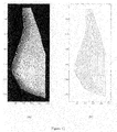
- FIG. 12 shows a mammogram (panel (a)) and a contour plot of a corresponding distance map (panel (b));
- FIG. 13 shows an ROC plot as a function of number of selected features selected using SFS with no stopping criterion for Polynomial Invariants and for 3-jet;
- FIG. 17 shows two sample mammograms and corresponding likelihood images using features [7 17 27 37 42 43]. Case (a) has an average pixel probability of 48.9% and case (b) 52.6%.
- the density refers to a specialist's assessment (typically a radiologist) of the projected area 2 of fibro glandular tissue—sometimes called dense tissue.
- FIGS. 2A to 2C respectively show three example mammograms depicting low, medium and high mammographic densities.
- a mammogram is classified into one of four or five density categories, e.g. Wolfe patterns and BI-RADS. These classifications are subjective and sometimes crude. They may be sufficient in some cases and for single measurements, but for serial, temporal analysis it is necessary to be able to detect more subtle changes.
- HRT treatment is known to increase breast density.
- the inventors have herein attempted to distinguish between an increase in breast density caused by HRT treatment and placebo populations.
- the inventors have used pattern recognition and data mining to enable the density measurement required to give an indicative result of increased risk of breast cancer.
- the first embodiment of the invention is based on the hypothesis that the breast tissue can be divided into subclasses describing its density. Each subclass should in theory relate to the anatomical composition of the surrounding breast tissue. Such labelling should be performed on the mammogram and each subclass should have some common statistical features. Following this, an unsupervised clustering algorithm with an appropriate similarity measure based on these features can be used to classify the subclasses in an unsupervised way.
- a region of interest is needed in which to estimate the mammographic density. Since the density is scattered in the interior breast tissue, a fairly rough segmentation along the boundary of the breast is sufficient.
- the process is illustrated in FIG. 4 . Delineation of the boundary may be done manually using 10 points along the boundary connected with straight lines resulting in a decagon region of interest as seen in the last panel of the figure. To ensure reproducible results, the same segmentation technique is applied to all images.
- the first step is to construct a Hessian matrix of partial derivatives based on the pixel intensities of the image.
- Hessian matrices will be well known to those skilled in the art, however, to summarise, a Hessian matrix is a matrix of second derivatives of a multivariate function, i.e. the gradient of the gradient of a function. Therefore, the Hessian matrix describes the second order intensity variations around each point of a 3D image.
- Gaussian derivatives are well known for their use in extracting features of computer images. Gaussian derivatives are used to extract features from the image at three different scales (in this example 1, 2 and 4 mm).
- ⁇ x i denotes partial differentiation along axis i
- ⁇ i is the order of differentiation for axis i
- * denotes convolution.
- the width of the Gaussian kernel determines the scale and the differentiation is carried out on this kernel prior to the convolution to get the scale space derivative.
- the Gaussian derivatives are derived so that it is possible to compare the characteristics of one pixel with its neighbour. For example, it is possible to determine which areas of the image have the same grey values by looking at the grey value of one pixel and comparing it to the grey value of the next pixel to work out a difference. If this is performed on a standard image, the results would be very sensitive to noise and there is a risk that the measurements would be impaired.
- the image is de-focused, i.e. blurred to minimise the noise. While this is preferable, it is of course appreciated that other methods may be used to achieve the same results. For example, the original image could be used with further processing that accounts for this additional noise.
- Gaussian derivatives also allows for a choice of scales i.e. a choice of to what extent the image is blurred.
- three different scale options are used, namely 1, 2 and 4 mm, although it will be appreciated that other scale values could possibly be used to achieve the same result.
- a Hessian matrix may be constructed.
- the eigenvalues of this matrix describe the local structure of the image.
- the Hessian matrix is constructed from the partial derivatives of the image:
- H ⁇ ( I ) [ ⁇ 2 ⁇ I ⁇ x 2 ⁇ 2 ⁇ I ⁇ x ⁇ ⁇ y ⁇ 2 ⁇ I ⁇ y ⁇ ⁇ x ⁇ 2 ⁇ I ⁇ y 2 ]
- I(x,y) is the image intensity at position (x,y).
- the combination of eigenvalues used as feature is the ratio
- this enables some mathematical definition of the characteristics of the structure, for example whether it is an elongated structure or not. For example, if there is a significant difference between L 1 and L 2 , this will be reflected in the magnitude of the resulting quotient value q s that gives an indication of the aspect ratio of tissue structures in the image. For example, if q s is large, then it will be clear that the shape is elongate. Conversely, if the magnitude of the resulting q s is small, then it implies that there is little difference between L 1 and L 2 and that the structure is more circular. The denominator of the equation allows normalisation of the quotient.
- the quotient measures the elongatedness in an image at a certain location (x,y) at the specific scale s. It is invariant to rotation of the image and scaling intensities.
- the outcome of the quotient value provides an indication of intensity of the structure. For example, a negative value indicates a dark elongated structure whereas a positive value indicates a bright elongated structure.
- Hessian at scale s is defined by:
- H s ⁇ ( I ) [ ⁇ s 2 ⁇ I ⁇ s ⁇ x 2 ⁇ s 2 ⁇ I ⁇ s ⁇ x ⁇ ⁇ s ⁇ y ⁇ s 2 ⁇ I ⁇ s ⁇ y ⁇ ⁇ s ⁇ x ⁇ s 2 ⁇ I ⁇ s ⁇ y 2 ]
- ⁇ s denotes the Gaussian derivative at scale s.
- the scales used are 1, 2 and 4 mm. The features used are given by the quotient:
- q s ⁇ e 1 ⁇ - ⁇ e 2 ⁇ ⁇ e 1 ⁇ + ⁇ e 2 ⁇
- e 1 and e 2 are eigenvalues of the Hessian at specific scale s and e 1 >e 2 .
- This ratio is related to the elongatedness of the image structure at the point (x,y) at the scale s that defines the image as having a “stripy” quality.
- this enables some mathematical definition of the characteristics of the structure, for example whether it is an elongated structure or not. For example, if there is a significant difference between e 1 and e 2 , this will be reflected in the magnitude of the resulting quotient value q s that gives an indication of the aspect ratio of tissue structures in the image. For example, if q s is large, then it will be clear that the shape is elongate. Conversely, if the magnitude of the resulting q s is small, then it implies that there is little difference between e 1 and e 2 and that the structure is more circular. The denominator of the equation allows normalisation of the quotient.
- the quotient measures the elongatedness in an image at a certain location (x,y) at the specific scale s. It is invariant to rotation of the image and scaling intensities.
- the outcome of the quotient value provides an indication of intensity of the structure. For example, a negative value indicates a dark elongated structure whereas a positive value indicates a bright elongated structure.
- K-means is a popular way to perform unsupervised clustering of data. It is employed to divide a mammogram into four structurally different areas (described below). Subsequently, based on the size of the areas, a density score is determined. As explained below, this score is a linear combination of areas that maximise the separation of HRT and placebo patients.
- FIG. 6 A visualisation of the threshold and stripiness methods is shown in FIG. 6 .
- Each quotient value is plotted in 3-dimensional space, where for each pixel, 3 quotient values are determined relating to the three different scales of Gaussian derivatives.
- the x-dimension may be used for 1 mm
- the y-dimension for quotient values determined at 2 mm
- the z-dimension for 4 mm.
- An example of this process is shown in FIG. 7 on a 2-dimensional axis.
- Three starting points 6 that are not too close to each other, within the three axes, are chosen at random. It should be appreciated that three points are chosen in this embodiment to result in three clusters. However, any number of starting points could be chosen depending on the desired number of clusters. In a preferred embodiment, four starting points would be selected.
- the algorithm below is then performed iteratively.
- the algorithm involves identifying for each quotient, which of the three random starting points is nearest. Each quotient is then effectively “affiliated” with the point to which it is closest and it is notionally classified as belonging to the same group. The same procedure is performed for each quotient, until each quotient belongs to one of the four starting points. For each resulting group of quotients, a mean is calculated and the mean quotient value is assigned as the new starting point 8 , thus resulting in three new starting points.
- the algorithm is performed iteratively until there is no change between the starting point and the resulting mean point. These three points 10 become the cluster points that will be used for future detection.
- cluster points may then be used to obtain a density score.
- a large collection of randomly chosen pixels from the different images in the data set are used to generate a representative collection of features.
- these features are divided into four clusters using k-means clustering.
- the means are stored and used for nearest mean classification.
- this nearest mean classifier is used to score each mammogram as follows:
- Hessian matrices are prepared for each Gaussian variable scale and quotient values obtained for each pixel. As there are three possible scales, each pixel has three different quotient values. The quotient values (for values of one scale at a time) are plotted alongside the four cluster means derived from the k-means clustering. Each quotient is assigned to the cluster mean that it is nearest to resulting in four real clusters. Each cluster mean will be representative of the different characteristics of the breast tissue. The result of classifying the pixels of an image into each of four classes is shown in FIG. 8 , one panel per class.
- the area of each cluster is determined and from this a score is obtained that utilises the difference in density between the different areas.
- the final score is based on a linear combination of the relative areas of the classes in the breast image. The optimum is determined using a linear discriminant analysis given the HRT group and the placebos. This optimal linear combination corresponds roughly to “2 ⁇ Area1 ⁇ 1 ⁇ Area2”.
- LDA linear discriminant analysis
- the two Areas 1 and 2 required for this calculation can be determined.
- the LDA determines which of the areas should be used for the above calculation based on the characteristics in the different clusters. This should be known to those in the art and will therefore not be further described herein.
- Each image in this new set consists of background and breast tissue that has been divided into four classes. These classes are tested as density measures separately and together using a linear classifier.
- a linear classifier is used because it generalises and is simple.
- the density score is the signed distance to the decision hyper-plane.
- the evaluation of the density measure is done in a leave one out approach.
- the linear classifier is trained on the N ⁇ 1 images and used to predict if the remaining image is from a HRT or a placebo patient.
- ROC Receiveiver Operating Characteristic
- p ⁇ ( w j ⁇ x ) p ⁇ ( x ⁇ w j ) ⁇ P ⁇ ( w j ) p ⁇ ( x )
- x) is known as the posterior probability
- w j ) the likelihood
- x) it is possible to ignore the common denominator. This leads to a decision function of the form d j ( x ) p ( x
- FIG. 9 Shown in FIG. 9 are the resulting ROC curves from using the described pattern recognition based density measure (“PR density”—circles) compared to the previously known adaptive threshold (“TH density”—diamonds) method. It shows that the PR density does a better job at classifying the patients into HRT and placebo groups. In terms of p-values the two measures are comparable, but again the PR-density is slightly better. When checking if the density means of the HRT group in 2001 is significantly higher than in 1999, the TH-measure yields a p-value of 0.002 and the PR measure 0.0002.
- PR density pattern recognition based density measure
- TH density diamonds
- unsupervised clustering of mammograms based on the quotient of Hessian eigenvalues at three scales result in tissue classes that can be used to differentiate between patients receiving HRT and patients receiving placebo. It is an automated method for measuring the effect of HRT as structural changes in the breast tissue. This measure can be interpreted as an intensity variant form of HRT induced structural density. Furthermore, the interactive threshold shows better capability to separate the HRT patients from the placebo patients at the end of the study than the categorising BI-RADS methodology.
- FIG. 3 the different effects are shown with respect to hormone replacement treatment and age.
- FIG. 3( a ) represents a probability density cloud for the patient groups receiving placebo and HRT at a start time t 0 and a later time t 2 respectively. Aging and HRT treatment are hypothesised to be two different effects.
- Breast cancer risk may be yet another dimension, as illustrated in FIG. 3( b ).
- the method described next is derived from observing the biological effect in a controlled study.
- the method is constructed to observe any one specific physiological effect and is invariant to affine intensity changes. Accordingly, digitised mammograms from an HRT study were examined in an example below to see if the effect of aging and HRT treatment are indeed two different effects.
- women were between 52 and 65 years of age, at least 1 year postmenopausal with a body mass index (BMI) less than or equal to 32 kg/m 2 .
- BMI body mass index
- HRT has been shown to increase mammographic density
- these images can be used to evaluate density measures by their ability to separate the HRT and placebo populations.
- aging effects can be detected by comparing the placebo group at t 0 and t 2 .
- the groups are donated as P 0 , P 2 , H 0 and H 2 for placebo and treatment at t 0 and t 2 respectively.
- the aim was to establish a new density measure based on data-mining of patient groups and machine learning. This approach is based directly on the image data and is as such independent of radiologist readings. It does require data expressing change in density and a selection of features to use.
- a pixel classifier is used, since it is desired to learn the local appearance of dense tissue.
- the large overlap between classes on pixel level both dense and non dense mammograms have many similar pixels, and also both dense and non dense mammograms appear in both the placebo and HRT population) disappears to a large degree when fusing the pixel probabilities to a single posterior for the image.
- Two collections of images are given together with a suitable feature space.
- Features are sampled in a large number of positions from each image. In this way each image is represented by a set of features.
- the sets are combined into two subgroups representing the collections A and B to provide a basis for classifier training.
- a nonlinear classifier is trained on this basis and used to compute probabilities of belonging to either A or B for all pixels in all images. These posteriors are then fused to one posterior probability for each image.
- the noise in the images is assumed to be uncorrelated point noise caused by a mixture of Poisson and Gauss processes.
- the presence of noise means one can not rely on pure analysis of isophotes and some robustness of the features with respect to which noise is needed.
- the density measure is derived by training a pixel classifier on subsets of image data in a supervised learning procedure.
- the subsets may respectively comprise images expected to have a lower density as one subset and images expected to have an increased density as a second subset.
- suitable subsets of interest include subsets devised such that there should be some detectable change in density.
- Subsets H 0 (group H at time t 0 ) and H 2 (group H at time t 2 ) are used to capture the effect of HRT. There is also an effect of aging, but it is expected to be much lower than that of HRT.
- the trained classifier is referred to as HRTL.
- Subsets P 2 placebo group P at time t 2
- H 2 are used to capture the effect of HRT. Separation between classes is expected to be lower, since inter-patient biological variability is diluting the results.
- the trained classifier is referred to as HRTC.
- the baseline population (P 0 (placebo group P at time t 0 ) and H 0 ) is stratified into three age groups, and the first and last tertile are used to capture the effects of age.
- the second tertile is used as control population.
- the trained classifier is referred to as AGE.
- Subsets P 0 and P 2 are used to capture any effect of non-affine, time dependent image changes. If no such changes are present in the images, this selection of subsets will also yield an age classifier.
- the trained classifier is referred to PlaL.
- kNN k nearest neighbours
- the classifier was trained on all but a pair of images (one image from each class) and pixel probabilities are computed for this pair using the trained classifier. This is repeated until all pixel probabilities for all images are computed.
- This technique is similar to leave-one-out, but is modified to leave-two-out since leaving one sample from class A out introduces a bias for belonging to class B, especially when the number of samples are relatively low (80 for the HRT classifiers and 56 for the age classifier).
- Feature vectors are extracted from 10,000 randomly selected pixels within the breast region in each image.
- FIG. 5 An example of a mammogram with corresponding pixel probability maps is shown in FIG. 5 .
- FIG. 5( a ) shows a mammogram from the data set described above
- FIGS. 5( b ), ( c ), and ( d ) show the pixel classification result using the classifiers HRTC, HRTL and AGE respectively.
- FIG. 6 illustrates the effect of automatic thresholding and “stripiness” and shows a) a starting mammogram, b) thresholded density, and c) the tissue clustering described above that is used to get the stripiness density.
- FIG. 10 shows the relative density changes using the three different training strategies. Specifically, FIG. 10 shows the relative longitudinal progression of the different measures.
- the placebo group is indicated with a dashed line and HRT by a solid line. Vertical bars indicate the standard deviation of the mean of the subgroups at t 2 and of the entire baseline population at t 0 .
- FIG. 11 examines if the differences between P 0 and P 2 indicated by the AGE and PlaL classifiers are indeed age effects or a difference in imaging at baseline and follow-up.
- the baseline population is stratified into three age groups.
- the PlaL measure shows neither an increasing trend nor significant difference in measurements.
- the aim of this example is to provide a framework for obtaining more accurate and sensitive measurements of breast density changes related to specific effects.
- Given effect-grouped patient data we propose a statistical learning scheme providing such a non-subjective and reproducible measure and compare it to the BI-RADS measure and a computer-aided percentage density.
- mammographic density i.e., the relative amount of fibroglandular tissue. Since the term mammographic density is most often used for this type of measure, we have decided to use “mammographic pattern” to describe more general properties of the mammogram. We mean to demonstrate that mammographic changes can perceived as a structural matter that may be accessed ignoring the actual brightness of the images and that it changes differently under the physiological processes of aging and HRT.
- women were between 52 and 65 years of age, at least 1 year postmenopausal with a body mass index less than or equal to 32 kg/m2.
- BI-RADS Breast imaging reporting and data system
- the BI-RADS categories are: 1) Entirely fatty; 2) Fatty with scattered broglandular tissue; 3) Heterogeneously dense; 4) Extremely dense.
- a trained radiologist assigns the mammogram to one of these categories based on visual inspection. It is included here since it is widely used both in clinical practice and for automated and computer aided approaches [22].
- the reading radiologist determines an intensity threshold using a slider in a graphical user interface. She is assisted visually by a display showing the amount of dense tissue corresponding to the current slider position.
- the system is similar to the approach proposed by Yaffe [11] and has been used in several clinical trials [22].
- the density is defined as the ratio between segmented dense tissue and total area of breast tissue.
- Our mammographic pattern measure is derived by training a pixel classifier on subsets of images from the available data. These subsets are chosen to represent the potential differences in patterns to be detected by the method. As an example, one subgroup may be the H 2 images from hormone treated patients and the other the P 2 images from the placebo group.
- the pixel classification would be based on local features that describe the image structure in the vicinity of every pixel to be classified.
- the features extracted per pixel will exhibit large similarity for every image even though they may come from two different subgroups of images. Therefore, for individual pixels, it will be difficult to decide to which of the subsets it belongs. Fusing all weak local decisions, however, into a global overall score per image ensures that sufficient evidence in favor of one of the two groups is accumulated and allows for a more accurate decision.
- the goal of feature selection in pattern recognition is to select the most discriminative features from a given feature set to improve classification performance.
- the first two improvements are of special interest to us, since we are ultimately interested in identifying the features most indicative of breast cancer risk.
- the aim of feature selection can be stated more formally as follows. Given a feature set F, we construct a classier with a recognition rate R(F) as a function of the selected features, F. The goal of feature selection is to select the subset F of F such that R(F)>R(T), where T denotes all possible subsets of F.
- R(F)>R(T) Several choices are available for quantifying the recognition rate, including specificity, sensitivity, area or volume overlap of a segmentation task, and area under ROC curve to name a few. Which choice to make depends on the application. It should be noted that, independent of choice, it is important to evaluate the recognition rate on data that are independent of the training data. This is typically done, either by splitting the data up in train and test sets or use a leave-one-out approach for evaluating the recognition rate [60].
- the gauge coordinate frame (v,w) is defined such that w is everywhere along the gradient direction and v tangential to the isophote. These two directions are always perpendicular to each other and form a local coordinate frame. All polynomial expressions in (v,w) are invariant under orthogonal transformations [1]. As one feature set we test all non-singular polynomial invariants up to third order resulting in 8 features per scale as shown in the following Table.
- the other tested feature set is the 3-jet consisting of all partial derivatives up to third order. This gives 10 features per scale.
- I xs G s * ⁇ I ⁇ x
- Gs denotes the Gaussian with standard deviation s.
- the numerical implementation takes advantage of the Fast Fourier Transform and the convolution is carried out through the Fourier domain [55].
- Both large feature sets are based on differential features related to image structure and the main difference is the rotational invariance provided by the invariant features. Only the best performing of the two sets are analysed in detail together with the stripiness features. We use scales 1, 2, and 4 mm based on previous findings with the stripiness features. In addition, a larger scale of 8 mm is introduced to allow for some larger scale information. This means we are testing 40 jet-features and 32 invariant features.
- the investigated mammograms are from the Dutch national breast cancer screening program.
- the data was originally used to investigate the effect of recall rate on earlier screen detection of breast cancers [68].
- Mammograms were collected from a total of 495 women participating in the biennial Dutch screening program. Of these, 250 were chosen as control subjects, and 245 were from women who were diagnosed with breast cancer.
- the data include screening mammograms from the time of diagnosis and screen-negative mammograms from at least two preceding screening examinations for both cases and controls.
- the data set used in this study was formed by selecting the earliest available screen-negative mammograms for all participants.
- the result is a high risk (100%) group of cases who were diagnosed with breast cancer within 2-4 years, but radiological reading provided no evidence of cancer at this earliest examination and 2 years after, and a low-risk group who were not diagnosed with breast cancer for a minimum of 4 following years.
- the segmentation of breast tissue was done automatically using techniques presented by Brady and Highnam [37] (breast boundary) and Karssemeijer [38] (pectoral muscle). Subsequently the masks were post processed using a morphological opening with a circular structure element with a diameter of 10 mm and the largest component selected as final breast tissue mask to improve the segmentation quality. Only the right mediolateral oblique (mlo) views are analysed in these experiments.
- the data is split up in a training and a test set, each consisting of 100 cancer and 100 control patients.
- Each component of each feature vector is normalized to unit variance across the entire training set.
- Standard sequential forward selection is used as feature selection algorithm with recognition rate quantified as area under ROC curve (AUC).
- AUC area under ROC curve
- the classification step is similar to what is described above, apart from the number of features used to represent each image.
- Machine memory only allowed 1000 feature vectors used per image due to the increase in feature space dimensionality and sample size.
- FIG. 13 shows the performance of SFS with no stopping criterion applied once using the invariance and position features and once using 3-jet and position. The same patients were used for train and test sets were used in both cases.
- FIGS. 14 , 15 and 16 show the results of the 100 runs of n-jet, n-jet+stripy selectable, and n-jet+stripy forced.
- the features from 1-10 are the 3-jet at scale 1 mm, from 11-20 the 3-jet at scale 2 mm, from 21-30 at 4 mm and 31-40 at 8 mm.
- the ordering of the 3-jet features is displayed in Table 1.
- Origo of the image coordinate system is in the upper left corner which means that the x-direction is vertical and the y-direction horizontal.
- Features 41-43 are the distance to skin line, horizontal displacement, and vertical displacement respectively.
- Features 44-46 are the stripiness features at scales 1, 2, and 4 mm.
- FIGS. 14 , 15 , and 16 give some information about the relationship between features and classes, which was one of the potential benefits of feature selection. Though a bit too flat to give a clear picture, it seems that the derivatives in the horizontal direction (2, 4, 7, 12, 14, . . . , 37), and the horizontal and vertical position (42 and 43) are the features most indicative of risk. 0th order features and pure vertical derivatives are very seldom selected. This may be the reason why the 3-jet performed better than the polynomial invariants—the orientation of structure matters.
- Case (a) is from a patient who had a screen-detected cancer in the right breast four years later.
- the BIRADS score of the mammogram is 3 but the likelihood score is quite low, 48.9% compared to an average of 50.2 ⁇ 0.9 for all the cases.
- Case (b) is an interval case also with a BIRADS score of 3 but a higher likelihood score, 52.6%.
- the histogram skewness was computed for all the images. This was the single feature found most related to risk in [63].
- the skewness is one of the features found related to mammographic density by Boone et al. [42] and is related to the degree of symmetry of the histogram.
- Huo et al. report an AUC of 0.82 ⁇ 0.04 for discrimination of 15 BRCA1/BRCA2 mutation carriers versus 143 ‘low-risk’ women. Classifying the images in the present study as cases or controls based on histogram skewness gave an AUC of 0.60. In comparison we on average get 0.70 ⁇ 0.03 with the selected cancer features.
Abstract
Description
- 1. Entirely fatty
- 2. Fatty with scattered fibroglandular tissue
- 3. Heterogeneously dense
- 4. Extremely dense.
L:
for any N-dimensional signal
f:
is defined by
and the variance t is the scale parameter. Based on this representation, scale space derivatives are defined by
where ∂x
where I(x,y) is the image intensity at position (x,y). The combination of eigenvalues used as feature is the ratio
where L1 is assigned the largest eigenvalue and L2 the smallest of the Hessian respectively, the absolute value of both is taken before the quotient above is determined. ε, a number much smaller than 1 is used to avoid instabilities associated with near zero division.
where ∂s denotes the Gaussian derivative at scale s. As set out above, the scales used are 1, 2 and 4 mm. The features used are given by the quotient:
where e1 and e2 are eigenvalues of the Hessian at specific scale s and e1>e2. This ratio is related to the elongatedness of the image structure at the point (x,y) at the scale s that defines the image as having a “stripy” quality.
| Initialize n, c, μ1, μ2, . . . , μc. | |
| repeat | |
| classify n samples according to nearest μi | |
| recompute μi |
| until no change in μi | |
| return μ1, μ2, . . . , μc | |
-
- Extract Hessian-based features
- Classify each pixel in one of four classes using the nearest mean classifier
- Determine relative areas of the classes
- Compute the score from those areas.
where p(wj|x) is known as the posterior probability, p(x|wj) the likelihood and P(wj) the prior. Since it is desired to compare probabilities and select the highest p(wj|x) it is possible to ignore the common denominator. This leads to a decision function of the form
d j(x)=p(x|w j)P(w j)
| Test | ||
| Method | P99 vs P01 | H99 vs H01 | P99 vs H99 | P01 vs H01 |
| BI-RADS | 0.3 | <0.001 | 0.3 | 0.1 |
| |
1 | <0.001 | 0.8 | 0.02 |
| Automatic TH | 0.07 | <0.001 | 0.8 | 0.2 |
| Stripiness | 0.9 | 0.004 | 0.9 | 0.02 |
- 1. Feature extraction: For all images, for preferably every pixel, at three scales, extract Hessian matrix and calculate the three “stripiness” quotients form those.
- 2. Clustering: Assign every feature vector of three quotients [or a large enough subset of these feature vectors] to one of K groups using K-means clustering; in particular, we take K=4.
- 3. Train classifier: determine the means of the K groups and associate one of K labels with every single one of the groups, i.e., we train a nearest mean classifier.
Test Phase [for a New Image or Image not Used in the Training Phase] - A. Feature extraction: For the image, for preferably every pixel, at the three same scales, extract Hessian matrix and calculate the same three “stripiness” quotients form those.
- B. Classification/labelling: Using the trained nearest mean classifier, assign one of the K=4 labels to every pixel based on its associated feature vector.
- C. “Density” score calculation: Determine the relative area in the breast for all of the K=4 classes and use the
rule 2×Area1−1×Area2
| Test | ||
| Method | P0 vs. P2 | H0 vs. H2 | P0 vs. H0 | P2 vs. H2 |
| BI-RADS | 0.3 | <0.001 | 0.3 | 0.1 |
| |
1 | <0.001 | 0.8 | 0.02 |
| HRTL | 0.08 | <0.001 | 0.7 | 0.01 |
| HRTC | 0.4 | <0.001 | 0.7 | 0.01 |
| Age | 0.004 | 0.4 | 0.8 | 0.07 |
| PlaL | 0.003 | <0.001 | 0.4 | 0.6 |
- 1. Feature extraction: For all images, for preferably every pixel, at three scales, extract Hessian matrix and calculate the three “stripiness” quotients form those.
- 2. Train at least one classifier:
Based on the stripiness features, the density measure is derived by training a pixel classifier on subsets of the available data. The subsets are devised such that there should be some detectable change indensity between them. Four combinations of subgroups are illustrated above.
In each case the two subgroups get a distinct label and a k nearest neighbours (kNN) classifier [22] is trained to separate pixels from the two classes.
Test Phase [for a New Image or Image not Used in the Training Phase] - A. Feature extraction: For the image, for every pixel, at the three same scales, extract Hessian matrix and calculate the same three “stripiness” quotients form those.
- B. Classification/labelling: Using the trained kNN classifier, assign a posterior probability to every pixel based on its associated feature vector.
The posterior probability, a number between 0 and 1, indicates how much a pixel belongs to one group or the other. For instance, in the specific example described above, if the HRTC classifier assigns a high posterior to a pixel, it indicates that this pixel “looks” like a pixel from an image in the HRT treated patient set. - C. “Density” score calculation: Determine the overall density score by averaging the posterior probabilities over the whole breast region. This average determines the score for that breast image. The score will be a number between 0 and 1. What this number indicates is of course dependent on which classifier is used: e.g. HRTL, HRTC, AGE, etc.
-
- Breast density is considered a structural property of the mammogram, that can change in various ways explaining different effects.
- The measure is derived from observing a specific effect in a controlled study.
- The measure is invariant to affine intensity changes.
-
- Improved classification performance.
- Better understanding of the relationship between features and classes.
- Less computing resources needed for building (and, depending of type, running) the classifier.
-
- Select the first feature that has the highest recognition rate among all features.
- Select the feature, among all unselected features, that gives the highest recognition rate together with the selected features.
- Repeat the previous step until you have reached a preset number of features, until the recognition rate exceeds a preset threshold, or until all features are selected.
| |
1 | 2 | 3 |
| Gauge | IwIw | IvvIw 2 | IvwIw 2 | IwwIw 2 | IvvvIw 3 | IvvwIw 3 | IvwwIw 3 | IwwwIw 3 |
where Gs denotes the Gaussian with standard deviation s. This is implemented by analytical derivation of the Gaussian prior to convolution using the fact that G*I=I*G [54]. The numerical implementation takes advantage of the Fast Fourier Transform and the convolution is carried out through the Fourier domain [55]. Both large feature sets are based on differential features related to image structure and the main difference is the rotational invariance provided by the invariant features. Only the best performing of the two sets are analysed in detail together with the stripiness features. We use
| TABLE 1 |
| The 3-jet features are ordered as follows. |
| Nr. | x | |
| 1 | 0 | 0 |
| 2 | 0 | 1 |
| 3 | 1 | 0 |
| 4 | 0 | 25 |
| 5 | 1 | 1 |
| 6 | 2 | 0 |
| 7 | 0 | 3 |
| 8 | 1 | 2 |
| 9 | 2 | 10 |
| 10 | 3 | 0 |
| This information is needed to read the feature indices of FIGS. 14, 15 and 16. | ||
- [1] B. M. ter Haar Romeny, L. M. J. Florack, A. H. Salden, and M. A. Viergever, “Higher order differential structure of images,” Image and Vision Computing, vol. 12, no. 6, pp. 317-325, July/August 1994.
- [11] J. W. Byng, N. F. Boyd, E. Fishell, R. A. Jong, and M. J. Yaffe, “The quantitative analysis of mammographic densities,” Physics in Medicine and Biology, vol. 39, p. 162938, 1994.
- [22] N. F. Boyd, J. M. Rommens, K. Vogt, V. Lee, J. L. Hopper, M. J. Yaffe, and A. D. Paterson, “Mammographic breast density as an intermediate phenotype for breast cancer,” The Lancet Oncology, vol. 5, pp. 798-808, 2005.
- [27] N. Boyd, L. Martin, Q. Li, L. Sun, A. Chiarelli, G. Hislop, M. Yaffe, and S. Minkin, “Mammographic density as a surrogate marker for the effects of hormone therapy on risk of breast cancer,” Cancer Epidemiology Biomarkers&Prevention, vol. 15, no. 5, p. 961, 2006.
- [28] M. H. Gail, L. A. Brinton, D. P. Byar, D. K. Corle, S. B. Green, C. Schairer, and J. J. Mulvihill, “Projecting individualized probabilities of developing breast cancer for white females who are being examined annually,” Journal of the National Cancer Institute, vol. 81, no. 24, pp. 1879-86, December 1989.
- [32] J. W. Byng, N. F. Boyd, E. Fishell, R. A. Jong, and M. J. Yaffe, “Automated analysis of mammographic densities,” Physics in Medicine and Biology, vol. 41, pp. 909-923, 1996.
- [37] R. Highnam and M. Brady, Mammographic Image Analysis, M. A. Viergever, Ed. Kluwer Academic Publishers, 1999.
- [38] N. Karssemeijer, “Automated classification of parenchymal patterns in mammograms,” Physics in Medicine and Biology, vol. 43, pp. 365-378, 1998.
- [42] J. M. Boone, K. K. Lindfors, C. S. Beatty, and J. A. Seibert, “A breast density index for digital mammograms based on radiologists' ranking,” Journal of Digital Imaging, vol. 11, no. 3, pp. 101-115, August 1998.
- [45] S. Petroudi and M. Brady, “Breast density segmentation using texture,” in International Workshop on Digital Mammography, S. M. Astley, M. Brady, C. Rose, and R. Zwiggelaar, Eds. Springer, 2006, pp. 609-615.
- [47] J. W. Byng, N. F. Boyd, L. Little, G. Lockwood, E. Fishell, R. A. Jong, and M. J. Yaffe, “Symmetry of projection in the quantitative analysis of mammographic images,” European Journal of Cancer Prevention, vol. 5, pp. 319-327, 1996.
- [54] J. J. Koenderink, “The structure of images,” Biological cybernetics, vol. 50, no. 5, pp. 363-370, 1984.
- [55] B. ter Haar Romeny, Front-End Vision and Multi-Scale Image Analysis. Kluwer Academic Publisher, 2003.
- [59] C. Tromans and M. Brady, “An alternative approach to measuring volumetric mammographic breast density,” in International Workshop on Digital Mammography, S. M. Astley, M. Brady, C. Rose, and R. Zwiggelaar, Eds. Springer, 2006, pp. 26-33.
- [60]A. K. Jain, R. P. W. Duin, and J. Mao, “Statistical pattern recognition: A review,” IEEETr. on PAMI, vol. 22, no. 1, pp. 4-37, 2000.
- [63] Z. Huo, M. Giger, D. Wolverton, W. Zhong, S. Cumming, and O. Olopade, “Computerized analysis of mammographic parenchymal patterns for breast cancer risk assessment: Feature selection,” Medical Physics, vol. 27, p. 4, 2000.
- [64] E. Claus, N. Risch, and W. Thompson, “Autosomal dominant inheritance of early-onset breast cancer implications for risk prediction.” Cancer, vol. 73, no. 3, pp. 643-51, 1994.
- [65] I. Guyon and A. Elisseeff, “An introduction to variable and feature selection,” The Journal of Machine Learning Research, vol. 3, pp. 1157-1182, 2003.
- [66] A. Whitney, “A direct method of nonparametric measurement selection,” in IEEETrans. Comput., vol. 20, 1971, pp. 1100-1103.
- [67] J. Koenderink and A. van Doorn, “Representation of local geometry in the visual system,” Biological Cybernetics, vol. 55, no. 6, pp. 367-375, 1987.
- [68] J. D. M. Otten, N. Karssemeijer, J. H. C. L. Hendriks, J. H. Groenewoud, J. Fracheboud, A. L. M. Verbeek, H. J. de Koning, and R. Holland, “Effect of recall rate on earlier screen detection of breast cancers based on the dutch performance indicators,” Journal of the National Cancer Institute, vol. 97, no. 10, pp. 748-754, May 2005.
Claims (21)
Priority Applications (3)
| Application Number | Priority Date | Filing Date | Title |
|---|---|---|---|
| US12/317,530 US8218850B2 (en) | 2006-02-10 | 2008-12-23 | Breast tissue density measure |
| PCT/IB2009/008098 WO2010143015A2 (en) | 2008-12-23 | 2009-12-23 | Breast tissue density measure |
| US12/787,703 US8285019B2 (en) | 2006-02-10 | 2010-05-26 | Breast tissue density measure |
Applications Claiming Priority (5)
| Application Number | Priority Date | Filing Date | Title |
|---|---|---|---|
| GB0602739.5 | 2006-02-10 | ||
| GBGB0602739.5A GB0602739D0 (en) | 2006-02-10 | 2006-02-10 | Breast tissue density measure |
| PCT/EP2007/051284 WO2007090892A1 (en) | 2006-02-10 | 2007-02-09 | Breast tissue density measure |
| US12/223,550 US8315446B2 (en) | 2006-02-10 | 2007-02-09 | Breast tissue density measure |
| US12/317,530 US8218850B2 (en) | 2006-02-10 | 2008-12-23 | Breast tissue density measure |
Related Parent Applications (3)
| Application Number | Title | Priority Date | Filing Date |
|---|---|---|---|
| US12/223,550 Continuation-In-Part US8315446B2 (en) | 2006-02-10 | 2007-02-09 | Breast tissue density measure |
| PCT/EP2007/051284 Continuation-In-Part WO2007090892A1 (en) | 2006-02-10 | 2007-02-09 | Breast tissue density measure |
| US22355009A Continuation-In-Part | 2006-02-10 | 2009-02-17 |
Related Child Applications (1)
| Application Number | Title | Priority Date | Filing Date |
|---|---|---|---|
| US12/787,703 Continuation-In-Part US8285019B2 (en) | 2006-02-10 | 2010-05-26 | Breast tissue density measure |
Publications (2)
| Publication Number | Publication Date |
|---|---|
| US20090232376A1 US20090232376A1 (en) | 2009-09-17 |
| US8218850B2 true US8218850B2 (en) | 2012-07-10 |
Family
ID=41063083
Family Applications (1)
| Application Number | Title | Priority Date | Filing Date |
|---|---|---|---|
| US12/317,530 Active 2029-06-26 US8218850B2 (en) | 2006-02-10 | 2008-12-23 | Breast tissue density measure |
Country Status (1)
| Country | Link |
|---|---|
| US (1) | US8218850B2 (en) |
Cited By (4)
| Publication number | Priority date | Publication date | Assignee | Title |
|---|---|---|---|---|
| US8483433B1 (en) * | 2009-09-17 | 2013-07-09 | Lockheed Martin Corporation | Detection of faint perturbations of interest using statistical models of image texture |
| KR20140057130A (en) * | 2012-10-25 | 2014-05-12 | 삼성전자주식회사 | Image processing system |
| US9466009B2 (en) | 2013-12-09 | 2016-10-11 | Nant Holdings Ip. Llc | Feature density object classification, systems and methods |
| US11386636B2 (en) | 2019-04-04 | 2022-07-12 | Datalogic Usa, Inc. | Image preprocessing for optical character recognition |
Families Citing this family (12)
| Publication number | Priority date | Publication date | Assignee | Title |
|---|---|---|---|---|
| GB0602739D0 (en) * | 2006-02-10 | 2006-03-22 | Ccbr As | Breast tissue density measure |
| JP5581574B2 (en) * | 2008-07-09 | 2014-09-03 | 富士ゼロックス株式会社 | Image processing apparatus and image processing program |
| GB2468164B (en) * | 2009-02-27 | 2014-08-13 | Samsung Electronics Co Ltd | Computer-aided detection of lesions |
| WO2011100511A2 (en) * | 2010-02-11 | 2011-08-18 | University Of Michigan | Methods for microcalification detection of breast cancer on digital tomosynthesis mammograms |
| US20120063656A1 (en) * | 2010-09-13 | 2012-03-15 | University Of Southern California | Efficient mapping of tissue properties from unregistered data with low signal-to-noise ratio |
| US8781187B2 (en) * | 2011-07-13 | 2014-07-15 | Mckesson Financial Holdings | Methods, apparatuses, and computer program products for identifying a region of interest within a mammogram image |
| US10102348B2 (en) * | 2012-05-31 | 2018-10-16 | Ikonopedia, Inc | Image based medical reference systems and processes |
| US10134148B2 (en) * | 2013-05-30 | 2018-11-20 | H. Lee Moffitt Cancer Center And Research Institute, Inc. | Method of assessing breast density for breast cancer risk applications |
| WO2014194160A1 (en) * | 2013-05-30 | 2014-12-04 | H. Lee Moffitt Cancer Center And Research Institute, Inc. | Automated percentage of breast density measurements for full field digital mammography |
| US9626476B2 (en) | 2014-03-27 | 2017-04-18 | Change Healthcare Llc | Apparatus, method and computer-readable storage medium for transforming digital images |
| WO2019183136A1 (en) * | 2018-03-20 | 2019-09-26 | SafetySpect, Inc. | Apparatus and method for multimode analytical sensing of items such as food |
| WO2020107023A1 (en) * | 2018-11-23 | 2020-05-28 | Icad, Inc | System and method for assessing breast cancer risk using imagery |
Citations (6)
| Publication number | Priority date | Publication date | Assignee | Title |
|---|---|---|---|---|
| WO2000079474A1 (en) | 1999-06-23 | 2000-12-28 | Qualia Computing, Inc. | Computer aided detection of masses and clustered microcalcification strategies |
| WO2003042712A1 (en) | 2001-11-13 | 2003-05-22 | Koninklijke Philips Electronics Nv | Black blood angiography method and apparatus |
| US20040151356A1 (en) | 2003-01-31 | 2004-08-05 | University Of Chicago | Method, system, and computer program product for computer-aided detection of nodules with three dimensional shape enhancement filters |
| JP2004313478A (en) | 2003-04-16 | 2004-11-11 | Mie Tlo Co Ltd | Medical image processing method |
| JP2005066194A (en) | 2003-08-27 | 2005-03-17 | Mie Tlo Co Ltd | Method for histological classification of calcification shadow |
| US20090296999A1 (en) | 2006-02-10 | 2009-12-03 | Nordic Bioscience Imaging A/S | Breast Tissue Density Measure |
-
2008
- 2008-12-23 US US12/317,530 patent/US8218850B2/en active Active
Patent Citations (8)
| Publication number | Priority date | Publication date | Assignee | Title |
|---|---|---|---|---|
| WO2000079474A1 (en) | 1999-06-23 | 2000-12-28 | Qualia Computing, Inc. | Computer aided detection of masses and clustered microcalcification strategies |
| WO2003042712A1 (en) | 2001-11-13 | 2003-05-22 | Koninklijke Philips Electronics Nv | Black blood angiography method and apparatus |
| US7020314B1 (en) * | 2001-11-13 | 2006-03-28 | Koninklijke Philips Electronics N.V. | Black blood angiography method and apparatus |
| US20040151356A1 (en) | 2003-01-31 | 2004-08-05 | University Of Chicago | Method, system, and computer program product for computer-aided detection of nodules with three dimensional shape enhancement filters |
| US6937776B2 (en) * | 2003-01-31 | 2005-08-30 | University Of Chicago | Method, system, and computer program product for computer-aided detection of nodules with three dimensional shape enhancement filters |
| JP2004313478A (en) | 2003-04-16 | 2004-11-11 | Mie Tlo Co Ltd | Medical image processing method |
| JP2005066194A (en) | 2003-08-27 | 2005-03-17 | Mie Tlo Co Ltd | Method for histological classification of calcification shadow |
| US20090296999A1 (en) | 2006-02-10 | 2009-12-03 | Nordic Bioscience Imaging A/S | Breast Tissue Density Measure |
Non-Patent Citations (26)
| Title |
|---|
| Boone J.M., et al., "A breast density index for digital mammograms basd on radiologists ranking", Journal of Digital Imaging, vol. 11, No. 3, pp. 101-115, Aug. 1998. |
| Boyd, N.F., et al., "Mammographic breast density as an intermediate phenotype for breast cancer", The Lancet Oncology, vol. 5, 00. 798-808, 2005. |
| Boyd, N.L., et al., "Mammographic density as a surrogate marker for the effects of hormone therapy on risk of breast cancer", Cancer Epidemiology Biomarkers & Prevention, vol. 15, No. 5, p. 961, 2006. |
| Byng, J.W., et al., "Automated analysis of mammographic densities,"Physics in Medicine and Biology, vol. 41, pp. 909-923, 1996. |
| Byng, J.W., et al., "Symmetry of projection in the quantitative anlaysis of mammographic images", European Journal of Cancer Prevention, vol. 5, pp. 319-327, 1996. |
| Byng, J.W., et al., "The quantitative analysis of mammographic densities,"Physics in Medicine and Biology, vol. 39, p. 1629-38, 1994. |
| Claus, E., et al., "Autosomal dominant inheritance of early-onset breast cancer, implications for risk prediction", Cancer, vol. 73, No. 3, pp. 643-651, 1994. |
| Gail, M.H., et al., "Projecting individualized probabilities of developing breast cancer for white females who are being examined annually", Journal of the National Cancer Institute, vol. 81, No. 24, pp. 1879-1886, Dec. 1989. |
| Guyon, I., et al., "An introduction to variable and feature selection", The Journal of Machine Learning Research, vol. 3, pp. 1157-1182, 2003. |
| Huo, Z. et al., "Computerized analysis of mammographic parenchymal patters for breast cancer risk assessment: Feature selection", Medical Physics, vol. 27, p. 4, 2000. |
| Jain, A.K., et al., "Statistical pattern recognition: A review", IEEETronPAMI, vol. 22, No. 1, pp. 4-37, 2000. |
| Karssemeijer, N., "Automated classification of parenchymal patterns in mammograms," Physics in Medicine and Biology, vol. 43, pp. 365-378, 1998. |
| Koenderink, J., et al., "Representation of local geometry in the visual system", Biological cybernetics, vol. 55, No. 6, pp. 367-375, 1987. |
| Koenderink, J.J., "The structure of images", Biological cybernetics, vol. 50, No. 5, pp. 363-370, 1984. |
| Otten, J.D.M., et al., "Effect of recall rate on earlier screen detection of breast cancers based on the dutch performance indicators", Journal of the National Cancer Institute, vol. 97, No. 10, pp. 748-754, May 2005. |
| Petroudi, S., et al., "Breast density segmentation using texture", in International Workshop on Digital Mammography, Astley, S.M., et al., Springer, 2006, pp. 609-615. |
| Pettersen P.C. , et al., "Parallel assessment of the impact of different hormone replacement therapies on breast density by radiologist and computer-based analyses of mammograms", Climacteric. Apr. 2008; 11(2): 135-43. |
| R. Nakayama et al., "Computer-aided diagnosis scheme for histological classification of clustered microcalcifications on magnification mammograms", Medical Physics, 31(4), pp. 789-799 (Apr. 2004). |
| R. Nakayama et al., "Development of New Filter Bank for Detectionof Nodular Patterns and Linear Patterns in Medical Images", Systems and Computers in Japan, 36(13), pp. 81-91 (2005). |
| Raundahl, J., dissertation, estimated publication date Dec. 26, 2007. |
| Raundahl, J., et al., "Automated Effect-specific Mammographic Pattern Measures", IEEE Transactions on Medical Imaging, vol. 27, No. 8, Aug. 2008 1054-1060. |
| Raundahl, J., et al., "Quantifying effect-specific mammographic density", Med Image Comput Assist Interv. 2007;10 (Pt 2): 580-7. |
| Romeny, Haar B.M. ter et al., "Higher order differential structure of images", Image and Vision Computing, vol. 12, No. 6, pp. 317-325, Jul./Aug. 1994. |
| Tromans C., et al., "An alternative approach to measuring volumetric mammographic breast density", in International Workshop on Digital Mammography, Astley, S.M. et al., Eds. Springer, 2006, pp. 26-33. |
| Whitney, A., et al., "A direct method of nonparametric measurement selection", in IEEETrans. Comput., vol. 20, 1971, pp. 1100-1103. |
| Zhou, et al., Medical physics 28(6), Jun. 2001, 1056-1069. |
Cited By (9)
| Publication number | Priority date | Publication date | Assignee | Title |
|---|---|---|---|---|
| US8483433B1 (en) * | 2009-09-17 | 2013-07-09 | Lockheed Martin Corporation | Detection of faint perturbations of interest using statistical models of image texture |
| KR20140057130A (en) * | 2012-10-25 | 2014-05-12 | 삼성전자주식회사 | Image processing system |
| KR102128325B1 (en) | 2012-10-25 | 2020-07-01 | 삼성전자주식회사 | Image Processing System |
| US9466009B2 (en) | 2013-12-09 | 2016-10-11 | Nant Holdings Ip. Llc | Feature density object classification, systems and methods |
| US9754184B2 (en) | 2013-12-09 | 2017-09-05 | Nant Holdings Ip, Llc | Feature density object classification, systems and methods |
| US10102446B2 (en) | 2013-12-09 | 2018-10-16 | Nant Holdings Ip, Llc | Feature density object classification, systems and methods |
| US10671879B2 (en) | 2013-12-09 | 2020-06-02 | Nant Holdings Ip, Llc | Feature density object classification, systems and methods |
| US11527055B2 (en) | 2013-12-09 | 2022-12-13 | Nant Holdings Ip, Llc | Feature density object classification, systems and methods |
| US11386636B2 (en) | 2019-04-04 | 2022-07-12 | Datalogic Usa, Inc. | Image preprocessing for optical character recognition |
Also Published As
| Publication number | Publication date |
|---|---|
| US20090232376A1 (en) | 2009-09-17 |
Similar Documents
| Publication | Publication Date | Title |
|---|---|---|
| US8218850B2 (en) | Breast tissue density measure | |
| US8315446B2 (en) | Breast tissue density measure | |
| US8285019B2 (en) | Breast tissue density measure | |
| Teramoto et al. | Fast lung nodule detection in chest CT images using cylindrical nodule-enhancement filter | |
| Campadelli et al. | A fully automated method for lung nodule detection from postero-anterior chest radiographs | |
| US20190108632A1 (en) | Advanced computer-aided diagnosis of lung nodules | |
| US7840062B2 (en) | False positive reduction in computer-assisted detection (CAD) with new 3D features | |
| US8687867B1 (en) | Computer-aided detection and classification of suspicious masses in breast imagery | |
| US20100183210A1 (en) | Computer-assisted analysis of colonic polyps by morphology in medical images | |
| US20180053297A1 (en) | Methods and Apparatuses for Detection of Abnormalities in Low-Contrast Images | |
| Tortajada et al. | Adapting breast density classification from digitized to full-field digital mammograms | |
| Loizidou et al. | Automatic breast mass segmentation and classification using subtraction of temporally sequential digital mammograms | |
| Carrillo-de-Gea et al. | A computer-aided detection system for digital chest radiographs | |
| WO2010143015A2 (en) | Breast tissue density measure | |
| Loizidou et al. | Benign and malignant breast mass detection and classification in digital mammography: the effect of subtracting temporally consecutive mammograms | |
| Raundahl et al. | Automated effect-specific mammographic pattern measures | |
| Sampat et al. | Classification of mammographic lesions into BI-RADS shape categories using the beamlet transform | |
| Karale et al. | Reduction of false positives in the screening CAD tool for microcalcification detection | |
| Zhao et al. | False positive reduction for lung nodule CAD using support vector machines and genetic algorithms | |
| Murphy et al. | Automated detection of pulmonary nodules from low-dose computed tomography scans using a two-stage classification system based on local image features | |
| Karahaliou et al. | A texture analysis approach for characterizing microcalcifications on mammograms | |
| Salman et al. | Breast Cancer Classification as Malignant or Benign based on Texture Features using Multilayer Perceptron | |
| KR101010927B1 (en) | Automated Polyps Detection Method using computer tomographic colonography and Automated Polyps Detection System using the same | |
| Giger | Computer-aided diagnosis in diagnostic mammography and multimodality breast imaging | |
| Raundahl et al. | Mammographic density measured as changes in tissue structure caused by HRT |
Legal Events
| Date | Code | Title | Description |
|---|---|---|---|
| AS | Assignment |
Owner name: NORDIC BIOSCIENCE IMAGING A/S, DENMARK Free format text: ASSIGNMENT OF ASSIGNORS INTEREST;ASSIGNOR:NORDIC BIOSCIENCE A/S;REEL/FRAME:022299/0325 Effective date: 20090211 |
|
| AS | Assignment |
Owner name: NORDIC BIOSCIENCE IMAGING A/S, DENMARK Free format text: ASSIGNMENT OF ASSIGNORS INTEREST;ASSIGNORS:RAUNDAHL, JAKOB;LOOG, MARCO;NIELSEN, MADS;REEL/FRAME:022767/0829;SIGNING DATES FROM 20090412 TO 20090417 Owner name: NORDIC BIOSCIENCE IMAGING A/S, DENMARK Free format text: ASSIGNMENT OF ASSIGNORS INTEREST;ASSIGNORS:RAUNDAHL, JAKOB;LOOG, MARCO;NIELSEN, MADS;SIGNING DATES FROM 20090412 TO 20090417;REEL/FRAME:022767/0829 |
|
| AS | Assignment |
Owner name: SYNARC INC., CALIFORNIA Free format text: ASSIGNMENT OF ASSIGNORS INTEREST;ASSIGNOR:NORDIC BIOSCIENCE IMAGING A/S, A.K.A. SYNARC IMAGING TECHNOLOGIES A/S;REEL/FRAME:026693/0479 Effective date: 20110401 |
|
| AS | Assignment |
Owner name: BANK OF AMERICA, N.A., AS ADMINISTRATIVE AGENT, WA Free format text: SECURITY AGREEMENT;ASSIGNOR:SYNARC INC.;REEL/FRAME:027282/0959 Effective date: 20111123 |
|
| STCF | Information on status: patent grant |
Free format text: PATENTED CASE |
|
| AS | Assignment |
Owner name: BANK OF AMERICA, N.A., AS ADMINISTRATIVE AGENT, CA Free format text: NOTICE OF SECURITY INTEREST IN PATENTS;ASSIGNOR:SYNARC INC.;REEL/FRAME:030157/0547 Effective date: 20130405 |
|
| AS | Assignment |
Owner name: SYNARC INC., CALIFORNIA Free format text: TERMINATION AND RELEASE OF SECURITY INTEREST IN U.S. PATENTS (REEL 027282, FRAME 0959);ASSIGNOR:BANK OF AMERICA, N.A., AS ADMINISTRATIVE AGENT;REEL/FRAME:030173/0902 Effective date: 20120405 |
|
| AS | Assignment |
Owner name: CREDIT SUISSE AG, AS SECOND LIEN COLLATERAL AGENT, Free format text: PATENT SECURITY AGREEMENT (SECOND LIEN);ASSIGNOR:SYNARC INC.;REEL/FRAME:032777/0066 Effective date: 20140310 Owner name: SYNARC INC., CALIFORNIA Free format text: TERMINATION AND RELEASE OF SECURITY INTEREST IN UNITED STATES PATENTS (RELEASES REEL 030157 FRAME 0547);ASSIGNOR:BANK OF AMERICA, N.A.;REEL/FRAME:032776/0402 Effective date: 20140310 Owner name: CREDIT SUISSE AG, AS FIRST LIEN COLLATERAL AGENT, Free format text: PATENT SECURITY AGREEMENT (FIRST LIEN);ASSIGNOR:SYNARC INC.;REEL/FRAME:032776/0798 Effective date: 20140310 |
|
| AS | Assignment |
Owner name: THE BANK OF NEW YORK MELLON, AS COLLATERAL AGENT, Free format text: SECURITY INTEREST;ASSIGNORS:BIOCLINICA, INC.;SYNARC INC.;REEL/FRAME:036596/0889 Effective date: 20150918 |
|
| FEPP | Fee payment procedure |
Free format text: PAT HOLDER NO LONGER CLAIMS SMALL ENTITY STATUS, ENTITY STATUS SET TO UNDISCOUNTED (ORIGINAL EVENT CODE: STOL); ENTITY STATUS OF PATENT OWNER: LARGE ENTITY |
|
| REMI | Maintenance fee reminder mailed | ||
| FPAY | Fee payment |
Year of fee payment: 4 |
|
| SULP | Surcharge for late payment | ||
| AS | Assignment |
Owner name: BIOCLINICA, INC., PENNSYLVANIA Free format text: RELEASE BY SECURED PARTY;ASSIGNOR:BANK OF NEW YORK MELLON;REEL/FRAME:040085/0965 Effective date: 20161020 Owner name: SYNARC INC., CALIFORNIA Free format text: RELEASE BY SECURED PARTY;ASSIGNOR:BANK OF NEW YORK MELLON;REEL/FRAME:040085/0965 Effective date: 20161020 Owner name: JEFFERIES FINANCE LLC, NEW YORK Free format text: FIRST LIEN SECURITY AGREEMENT;ASSIGNORS:BIOCLINICA, INC.;SYNARC INC.;REEL/FRAME:040458/0800 Effective date: 20161020 Owner name: SYNARC, INC., CALIFORNIA Free format text: RELEASE OF SECOND LIEN SECURITY;ASSIGNOR:CREDIT SUISSE AG, CAYMAN ISLANDS BRANCH;REEL/FRAME:040458/0849 Effective date: 20161020 Owner name: BIOCLINICA, INC., PENNSYLVANIA Free format text: RELEASE OF FIRST LIEN SECURITY;ASSIGNOR:CREDIT SUISSE AG, CAYMAN ISLANDS BRANCH;REEL/FRAME:040458/0915 Effective date: 20161020 Owner name: SYNARC, INC., CALIFORNIA Free format text: RELEASE OF FIRST LIEN SECURITY;ASSIGNOR:CREDIT SUISSE AG, CAYMAN ISLANDS BRANCH;REEL/FRAME:040458/0915 Effective date: 20161020 Owner name: BIOCLINICA, INC., PENNSYLVANIA Free format text: RELEASE OF SECOND LIEN SECURITY;ASSIGNOR:CREDIT SUISSE AG, CAYMAN ISLANDS BRANCH;REEL/FRAME:040458/0849 Effective date: 20161020 Owner name: JEFFERIES FINANCE LLC, NEW YORK Free format text: PATENT SECURITY AGREEMENT;ASSIGNORS:BIOCLINICA, INC.;SYNARC INC.;REEL/FRAME:040458/0810 Effective date: 20161020 |
|
| AS | Assignment |
Owner name: BIOCLINICA, INC., NEW JERSEY Free format text: ASSIGNMENT OF ASSIGNORS INTEREST;ASSIGNOR:SYNARC INC.;REEL/FRAME:048468/0743 Effective date: 20190221 |
|
| MAFP | Maintenance fee payment |
Free format text: PAYMENT OF MAINTENANCE FEE, 8TH YEAR, LARGE ENTITY (ORIGINAL EVENT CODE: M1552); ENTITY STATUS OF PATENT OWNER: LARGE ENTITY Year of fee payment: 8 |
|
| AS | Assignment |
Owner name: BIOCLINICA, INC., PENNSYLVANIA Free format text: SECOND LIEN RELEASE OF SECURITY INTEREST IN PATENTS;ASSIGNOR:JEFFERIES FINANCE LLC, AS COLLATERAL AGENT;REEL/FRAME:056064/0563 Effective date: 20210427 Owner name: BIOCLINICA, INC., PENNSYLVANIA Free format text: FIRST LIEN RELEASE OF SECURITY INTEREST IN PATENTS;ASSIGNOR:JEFFERIES FINANCE LLC, AS COLLATERAL AGENT;REEL/FRAME:056064/0341 Effective date: 20210427 |
|
| AS | Assignment |
Owner name: GOLDMAN SACHS BANK USA, AS COLLATERAL AGENT, NEW YORK Free format text: FIRST LIEN SECURITY AGREEMENT;ASSIGNOR:BIOCLINICA, INC.;REEL/FRAME:063123/0066 Effective date: 20230320 |
|
| AS | Assignment |
Owner name: GOLDMAN SACHS BANK USA, AS COLLATERAL AGENT, NEW YORK Free format text: SECOND LIEN SECURITY AGREEMENT;ASSIGNOR:BIOCLINICA, INC.;REEL/FRAME:063141/0589 Effective date: 20230320 |
|
| MAFP | Maintenance fee payment |
Free format text: PAYMENT OF MAINTENANCE FEE, 12TH YEAR, LARGE ENTITY (ORIGINAL EVENT CODE: M1553); ENTITY STATUS OF PATENT OWNER: LARGE ENTITY Year of fee payment: 12 |