US7808903B2 - System and method of forecasting usage of network links - Google Patents
System and method of forecasting usage of network links Download PDFInfo
- Publication number
- US7808903B2 US7808903B2 US12/054,726 US5472608A US7808903B2 US 7808903 B2 US7808903 B2 US 7808903B2 US 5472608 A US5472608 A US 5472608A US 7808903 B2 US7808903 B2 US 7808903B2
- Authority
- US
- United States
- Prior art keywords
- data values
- processor
- traffic data
- peak traffic
- network
- Prior art date
- Legal status (The legal status is an assumption and is not a legal conclusion. Google has not performed a legal analysis and makes no representation as to the accuracy of the status listed.)
- Active, expires
Links
Images


Classifications
-
- H—ELECTRICITY
- H04—ELECTRIC COMMUNICATION TECHNIQUE
- H04L—TRANSMISSION OF DIGITAL INFORMATION, e.g. TELEGRAPHIC COMMUNICATION
- H04L41/00—Arrangements for maintenance, administration or management of data switching networks, e.g. of packet switching networks
- H04L41/14—Network analysis or design
- H04L41/147—Network analysis or design for predicting network behaviour
-
- H—ELECTRICITY
- H04—ELECTRIC COMMUNICATION TECHNIQUE
- H04L—TRANSMISSION OF DIGITAL INFORMATION, e.g. TELEGRAPHIC COMMUNICATION
- H04L41/00—Arrangements for maintenance, administration or management of data switching networks, e.g. of packet switching networks
- H04L41/14—Network analysis or design
- H04L41/142—Network analysis or design using statistical or mathematical methods
Definitions
- Packet data networks e.g. internet protocol (IP) networks
- IP internet protocol
- the level of traffic e.g. voice, video, data, etc.
- IP networks must attempt to ensure both quality of service (QoS) guarantees for services provided, and service level agreement (SLA) requirements to customers.
- IP networks must be able to adapt to changing trends in traffic on the network in order to efficiently utilize resources of the network, and ensure QoS and satisfy SLA requirements.
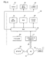
- FIG. 1 is a system diagram of a network monitoring system connected to a multi-service network providing service to customers, according to an exemplary embodiment
- FIG. 2A is a flow chart of a process for forecasting future usage of a network, according to an exemplary embodiment
- FIG. 2B is a flow chart of a process for adjusting the forecast of future usage of the network, according to an exemplary embodiment
- FIG. 3 is a graph depicting actual traffic data of a network link in percentage utilization of the network link over time, and overlaid with a trend curve used to forecast peak traffic requirements for the network link using actual data and a proposed trend curve used to forecast peak traffic requirements of the network link using modified data, according to an exemplary embodiment;
- FIG. 4B is a graph including the same actual data traffic curve and trend curve as represented in FIG. 4A , overlaid with a proposed trend curve that has been further modified as compared to FIG. 4A , according to an exemplary embodiment;
- FIG. 5A is a graph depicting actual traffic data of yet another network link in percentage utilization of the network link over time, and overlaid with a trend curve used to forecast peak traffic requirements for the network link using actual data and a proposed trend curve used to forecast peak traffic requirements of the network link using modified data, according to an exemplary embodiment;
- FIG. 5B is a graph including the same actual data traffic curve and trend curve as represented in FIG. 5A , overlaid with a proposed trend curve that has been further modified as compared to FIG. 5A , according to an exemplary embodiment;
- FIG. 6A is a graph depicting actual traffic data of a further network link in percentage utilization of the network link over time, and overlaid with a trend curve used to forecast peak traffic requirements for the network link using actual data and a proposed trend curve used to forecast peak traffic requirements of the network link using modified data, according to an exemplary embodiment;
- FIG. 6B is a graph including the same actual data traffic curve and trend curve as represented in FIG. 6A , overlaid with a proposed trend curve that has been further modified as compared to FIG. 6A , according to an exemplary embodiment;
- FIG. 7 is a graph depicting actual traffic data of a still further network link in percentage utilization of the network link over time, and overlaid with a trend curve used to forecast peak traffic requirements for the network link using actual data and a proposed trend curve used to forecast peak traffic requirements of the network link using modified data, according to an exemplary embodiment
- FIG. 8 is a diagram of a computer system that can be used to implement various exemplary embodiments.
- various computer networks are used to interconnect computing devices (personal computers, workstations, peripheral devices, etc.) for use in both personal and business settings.
- Businesses may utilize computer networks that cover broad geographical areas and utilize a collection of computer networking devices (e.g., routers, switches, hubs, etc.) for use by their employees and to interconnect various remote offices.
- various service providers may provide multiple services to customers for entertainment or business-related reasons through devices capable of processing signals for presentation to a customer, such as a set-top box (STB), a home communication terminal (HCT), a digital home communication terminal (DHCT), a stand-alone personal video recorder (PVR), a television set, a digital video disc (DVD) player, a video-enabled phone, a video-enabled personal digital assistant (PDA), and/or a personal computer (PC), as well as other like technologies and customer premises equipment (CPE).
- STB set-top box
- HCT home communication terminal
- DHCT digital home communication terminal
- PVR stand-alone personal video recorder
- DVD digital video disc
- PDA video-enabled personal digital assistant
- PC personal computer
- CPE customer premises equipment
- a multi-service network can be used by a service provider to provide customers with augmented data and/or video content to provide, e.g., sports coverage, weather forecasts, traffic reports, commentary, community service information, etc., and augmented content, e.g., advertisements, broadcasts, video-on-demand (VOD), interactive television programming guides, links, marketplace information, etc.
- augmented content e.g., advertisements, broadcasts, video-on-demand (VOD), interactive television programming guides, links, marketplace information, etc.
- IP internet protocol
- Such a multi-service network could also be used to provide the customer with the ability to use the network as a telephone using voice over internet protocol (VOIP) transmissions.
- IP internet protocol
- VOIP voice over internet protocol
- Network links used to carry the information traffic throughout the network by nature have limited capacity to carry traffic.
- Network operators can configure the network (e.g., by adding links, by replacing a link with a link of increased capacity, etc.) in such a way as to increase the overall capacity of the network; however, due to the costs associated with increased capacity, it is desirable to not unnecessarily increase capacity.
- Another factor that the network operators must consider when configuring the network is the need to provide services to customers in a manner that assures integrity of the information being transmitted and quality of the service being provided to the customer.
- FIG. 1 is a diagram of a system capable of monitoring a network in order to collect data regarding usage of the network, and analyze and accurately forecast future usage of the network.
- a network 101 is depicted, such as a multi-service network that can carry voice, video, and/or data traffic from one or more service providers to one or more customers.
- the network 101 serves service provider 1 121 , service provider 2 123 , . . . , and service providers 125 , where Y is the total number of service providers, as well as customer network, 103 , customer network 2 105 , . . . , and customer network N 107 , where N is the total number of customer networks.
- a network monitoring system 111 is connected to the network 101 in order to monitor the network, collect usage data, and analyze the usage data to forecast future usage using an analysis module 113 .
- the network monitoring system 111 can interface with or incorporate a data storage 115 that is used to store usage (traffic) data collected by the network monitoring system 111 from the network 101 .
- the network monitoring system 111 can also interface with or incorporate an SLA database 117 and a QoS database 119 , which can be used to assess whether the network 101 is satisfying SLA requirements and/or QoS guarantees, respectively.
- system 111 can be used to monitor and analyze multiple networks 101 .
- the data collection and analysis can be performed concurrently, wherein the data is stored and analyzed by the system for each particular network, or for each service provider and/or customer utilizing each particular network.
- service provider networks such as multi-service internet protocol (IP) networks
- IP networks must be sized based on peak traffic requirements, and not based on the average traffic levels measured over some period of time.
- IP networks must be able to adapt to changing trends in peak traffic requirements in order to efficiently utilize resources of the network, and ensure QoS and satisfy SLA requirements.
- Physical changes to the network such as upgrading of network link hardware, the addition of new network links, etc., that are needed to respond to changes in peak traffic requirements of the network require planning and time to implement.
- forecasting of future peak traffic requirements is a critical task for network operators.
- Network elements (NEs) and connecting fibers/cables/links are sized based on such forecasts, and need to be ordered and installed well in advance.
- a database of traffic rates for each network link can be collected and organized into given time ranges in the data storage 115 for further analysis by the analysis module 113 .
- a database of traffic rates of the link can be collected for each day, or for each week, etc., for the analysis of a peak traffic rate, or an average traffic rate, etc. for that time range.
- a database containing traffic rates for each day would include 288 data points for traffic rates if the collection interval over the day is every 5 minutes, or 96 data points for traffic rates if the collection interval over the day is every 15 minutes.
- the analysis module 113 can determine a peak traffic rate for each particular day for this link by finding the largest traffic rate value for that day.
- peak traffic rates can be determined for each week, or each month, etc., or even for each hour if finer granularity of analysis is desired.
- E is calculated by adding up the squares of the errors at each of the observed points. (Squaring is done to eliminate cancellations among errors with different signs).
- E ( f ( x 1 ) ⁇ y 1 ) 2 +( f ( x 2 ) ⁇ y 2 ) 2 + . . . +( f ( x m ) ⁇ y m ) 2 .
- x 1 , y 1 . . . y m are the observed data sets.
- a first order function i.e., a straight line function
- Methods such as mainly a Gaussian method, are used to solve the above equations and get the values of c 1 and c 2 .
- too few data points i.e., the historical data used in the forecast analysis does not extend over a sufficient range of time
- the use of a range of historical data that is between 10 and 20 weeks or months has proven to be effective in many instances for forecasting usage trends for network links.
- the network links need to be planned to handle peak traffic and not the average of some values.
- the algorithm used is developed to forecast peak traffic growth in the future based on currently available historical data.
- FIG. 2A sets forth a flowchart for a process for forecasting future traffic/usage of a network.
- the network monitoring system 111 performs regular auditing of the network 101 to collect traffic data and store the data in the data storage 115 .
- the analysis module 113 can compile a historical data set of peak values of the traffic data for a predetermined range of time, as set forth in step 203 .
- the analysis module 113 can review the traffic data values taken during each day (or hour, or week, or month, etc.) and find a peak traffic value for each day, and compile a historical data set over a twelve week range of time that contains a peak traffic value for each day during that twelve week period.
- the analysis module 113 applies a confidence factor to the peak traffic values in the historical data set to achieve modified data values (i.e., the values labeled as “confidence factor applied” in the tables). Then, in step 207 , the analysis module 113 applies a time-based weighting factor to the modified data values to achieve further modified data values (i.e., the values labeled as “time weighting factor applied” in the tables). The analysis module 113 then uses a method such as the Method of Least Squares to calculate a forecast trend curve (labeled as “proposed trend” in the tables and figures) of the traffic over the network 101 using the further modified data values and the forecast trend curve is output for use thereof, as set forth in step 209 .
- a method such as the Method of Least Squares to calculate a forecast trend curve (labeled as “proposed trend” in the tables and figures) of the traffic over the network 101 using the further modified data values and the forecast trend curve is output for use thereof, as set forth in step 209 .
- the resulting forecast trend curve and network capacity information can be compared with SLA requirements in the SLA database 117 and QoS guarantees in the QoS database 119 to determine whether the forecast includes growth that will require modification of the network configuration in order to meet the growth, and satisfy SLA requirements and QoS guarantees.
- the forecasting algorithm can be updated from time to time in order to obtain a better understanding of, and possibly make adjustments to, the confidence factors and time-based weighting factors needed to effectively use the traffic forecasting algorithm. By fine-tuning the confidence factors and/or the time-based weighting factor, the traffic forecasting algorithm can achieve a much closer fit towards meeting the peak traffic requirements.
- FIG. 2B is a flow chart of a process for adjusting the forecast of future usage of the network, according to an exemplary embodiment.
- the network monitoring system 111 continues to perform regular auditing of the network 101 to collect traffic data and store the data in the data storage 115 , even after the forecast trend curve is generated in order to verify the accuracy thereof.
- the actual data values are compared to the forecast trend curve, and then in step 213 the time-based weighting factor can be adjusted based on the comparison (e.g., see the examples below described with respect to Tables 3 and FIG. 4B , Table 5 and FIG. 5B , and Table 7 and FIG. 6B ).
- step 215 the historical data set is updated with the most-recent twelve weeks of traffic data
- the analysis module 113 applies the confidence factor to the updated historical data set to achieve modified data values.
- step 217 the analysis module 113 applies the adjusted time-based weighting factor to the modified data values to achieve further modified data values
- step 219 the analysis module 113 then uses a method such as the Method of Least Squares to recalculate a forecast trend curve using the further modified data values and the recalculated forecast trend curve is output for use thereof.
- the forecast algorithm can also take into account additional factors that influence the traffic growth itself, for example, the type of services using the link, and/or the number of customers allocated to the link. Thus, adjustments can be made to the parameters of the traffic algorithm so that the traffic forecasting algorithm can achieve a much closer fit towards meeting the peak traffic requirements.
- the forecast algorithm can be used to forecast the traffic growth of video services separately from the traffic growth of other services using the link, and then merge the growth forecast data of the video services with the growth forecast for other services. Otherwise, the growth rate of high bandwidth services, like video services, would remain masked among the other traffic, and when there is a sudden spurt in the growth rate of the video services the network operators would be taken by surprise.
- the forecast algorithm can be used to calculate growth forecasts for individual services where necessary, and incorporate the forecast results of those services into the overall traffic growth forecast over a network link.
- the number of customers allocated to the link it is general industry practice to allocate to a customer a certain maximum bandwidth based on the customer tier. Depending on the technology, this customer bandwidth could be allocated as a small pipe in a larger pipe (i.e., network link). The smaller pipes could be PVC, VLAN, etc. As more and more customers are added to the link, the traffic over the link would grow. However, when the link reaches its maximum customer (or PVC/VLAN) limit, the traffic growth would slow down, since additional traffic would come only from existing customers.
- the forecast algorithm can take this phenomenon into account by incorporating therein a correlation coefficient representative of the number of customers (or PVC/VLAN) with traffic. When the maximum customer limit is reached, the correlation coefficient can be removed, thus deducting this influence, in order to achieve a realistic forecast of future traffic.
- the forecast algorithm set forth herein is applicable to all types of networks and services where the requirement is to meet the peak traffic at any time.
- the forecast algorithm can be used for any type of network that carries any type of traffic, such as voice, video, data, etc.
- the algorithm provides an easy-to-use and logical method to forecast peak traffic growth.
- the algorithm is fine-tunable by adjusting two values, namely a confidence factor and a time-based weighting factor.
- the values for these factors are derived from the historical data itself.
- the algorithm can take into account other influencing factors like the type of service, the number of customers, etc., thereby improving the accuracy of traffic growth forecast.
- the forecast algorithm can be used to analyze networks that include thousands of NEs and links.
- five examples of network links are analyzed using the forecast algorithm to demonstrate the validity of the algorithm, and the collected and calculated data from these five examples are set forth in Tables 1-8 (set forth and discussed in greater detail below), and correspondingly depicted in FIGS. 3 , 4 A-B, 5 A-B, 6 A-B, and 7 .
- These examples use 12 weeks of actual usage data to prepare the forecast trend, and then overlay and compare the subsequent 12 weeks of actual usage data with the forecast trend in order to demonstrate the validity of the forecast trend.
- actual traffic data is collected over a period of 24 weeks using appropriate collection intervals.
- Tables 1-8 and FIGS. 3 , 4 A-B, 5 A-B, 6 A-B, and 7 represent the actual traffic data as a percentage of utilization of the network link capacity.
- only the data points for the first 12 weeks i.e., weeks 1-12
- the forecasted traffic is then compared against the actual data observed for weeks 13-24 in order to verify the algorithm used to generate the forecast.
- the forecast extends for 12 weeks into the future.
- the historical data range and forecast period can be changed depending upon the needs of the network link being analyzed.
- the forecast can be updated periodically, for example, every week or every other week, etc. using updated traffic data, and/or adjusted weighting factors, as will be discussed below.
- x is the weeks (from 1 to 12)
- y and Y are the unmodified and modified traffic (in percentage utilization)
- c is the confidence factor.
- a time-based weighting factor is also applied to the traffic data. It should be noted that the time-based weighting factor is applied to the traffic data that is already normalized by application of the confidence factor.
- the time-based weighting factor is applied to the traffic data in the history period, which in this case is the first 12 data points.
- the data that is more current is an indication of the recent trend or pattern of traffic utilization (growth, decline, or steady), and thus the more current data is weighted more than older data.
- This weighting factor is applied proportionately over the history period.
- each data point gets a weight based on its timewise distance from the origin data point (i.e., first data point in the historical data being evaluated). The further the data point is from the origin data point, the greater the weight given to the data point.
- An example is a weighting factor of 1.2.
- x is the weeks (from 1 to 12)
- Y is the value discussed above
- Y 1 is the final modified value.
- the Method of Least Squares is then used on the resulting final modified values to fit a forecasting curve, which is labeled in the tables and figures as the “proposed trend.”
- Tables 1-8 set forth below show results of the above analysis and calculations for the five examples.
- Table 1-8 show the data values for weeks 1-12 modified with the confidence factor applied, and then further modified with the time-based weighting factor applied, which are then used to generate the proposed trend curve using the method of least squares.
- Table 1 set forth below shows results of the above analysis and calculations for the first example, and FIG. 3 is a corresponding graph of the results.
- the average percentage utilization of the percentage utilization values for weeks 1-12 in Table 1 and FIG. 3 is 13.74858333 and the standard deviation is 3.483337805.
- the proposed trend curve made using the modified data extends above the trend curve made with actual data. While the trend curve made with actual data is clearly below many of the peaks in the actual data curve, the proposed trend curve meets all the forecast growth points without much over-shoot. Note that, at the time the forecast analysis will be performed, the actual data for weeks 13-24 will not yet be known; however, the comparison of the trend curve and the proposed trend curve in weeks 13-24 with the actual data of weeks 13-24 in the five examples allows for a checking of the accuracy of the forecast, and validation of the forecasting approach being used. As can be seen in FIG.
- the proposed trend curve provides a much better forecast of the growth of the usage of the network link being analyzed over weeks 13-24, as compared to the trend curve made with raw data values, which misses many peaks and would result in a failure to ensure QoS guarantees and meet SLA requirements for that link.
- Tables 2 and 3 set forth below show results of the analysis and calculations for the second example, and FIGS. 4A and 4B are corresponding graphs of the results.
- the average percentage utilization of the percentage utilization values for weeks 1-12 in Tables 2 and 3 and FIGS. 4A and 4B is 42.295 and the standard deviation is 4.995407891.
- the proposed trend curve made using the modified data extends above the trend curve made with raw actual data.
- the trend curve made with actual data is clearly below all of the peaks in the actual data curve, and in fact forecasts a downward trend in usage, which is clearly an error as can be seen in the growth shown in weeks 13-24.
- the proposed trend curve misses some of the peaks, the proposed trend curve is much closer to the peaks than the trend curve made with the raw actual data.
- the data in this example pertains to a case of a fast growing network. In such situations, the proposed trend curve can be adjusted to meet the peaks by suitably adjusting (e.g. increasing) the time-based weighting factor. Table 3 and FIG.
- Tables 4 and 5 set forth below show results of the analysis and calculations for the third example, and FIGS. 5A and 5B are corresponding graphs of the results.
- the average percentage utilization of the percentage utilization values for weeks 1-12 in Tables 4 and 5 and FIGS. 5A and 5B is 38.6525 and the standard deviation is 5.258145413.
- the proposed trend curve made using the modified data extends above the trend curve made with raw actual data.
- the trend curve made with actual data is clearly below all of the peaks in the actual data curve. While the proposed trend curve misses some of the peaks, the proposed trend curve is much closer to the peaks than the trend curve made with the raw actual data.
- the proposed trend curve is adjusted to meet the peaks by suitably adjusting (e.g. increasing) the time-based weighting factor.
- Table 5 and FIG. 5B show the effect of increasing the time-based weighting factor from 1.2 (as in Table 4 and FIG. 5A ) to 1.3 (as in Table 5 and FIG. 5B ).
- the proposed trend curve is able to closely meet the peaks over weeks 13-24.
- Tables 6 and 7 set forth below show results of the analysis and calculations for the fourth example, and FIGS. 6A and 6B are corresponding graphs of the results.
- the average percentage utilization of the percentage utilization values for weeks 1-12 in Tables 6 and 7 and FIGS. 6A and 6B is 63.43916667 and the standard deviation is 6.110877721.
- the proposed trend curve made using the modified data extends above the trend curve made with raw actual data.
- the trend curve made with actual data is clearly below some of the peaks in the actual data curve.
- the proposed trend curve meets all of the peaks, and in fact produces an over-build of the network link.
- the proposed trend curve can be downwardly adjusted to reduce over-build by suitably adjusting (e.g. decreasing) the time-based weighting factor, as shown in Table 7 and FIG. 6B .
- FIG. 6B show the effect of decreasing the time-based weighting factor from 1.2 (as in Table 6 and FIG. 6A ) to 1.1 (as in Table 7 and FIG. 6B ).
- the time-based weighting factor is decreased to 1.1, the proposed trend curve is able to meet the peaks over weeks 13-24 while reducing over-build of the network link.
- Table 8 set forth below shows results of the above analysis and calculations for the fifth example, and FIG. 7 is a corresponding graph of the results.
- the average percentage utilization of the percentage utilization values for weeks 1-12 in Table 8 and FIG. 7 is 37.21 and the standard deviation is 4.425451184.
- the proposed trend curve made using the modified data extends above the trend curve made with actual data, which actually shows a downward trend. While the trend curve made with actual data is clearly below the peaks in the actual data curve, the proposed trend curve meets all the forecast growth points without much over-shoot. As can be seen in FIG. 7 with respect to the fifth example, the proposed trend curve provides a much better forecast of the growth of the usage of the network link being analyzed over weeks 13-24, as compared to the trend curve made with raw data values, which misses many peaks and would result in a failure to ensure QoS guarantees and meet SLA requirements for that link.
- the traffic forecasting algorithm set forth above is able to correctly trend the traffic utilization to meet the peak requirements as against trending with raw actual data.
- the computer system 800 may be coupled via the bus 801 to a display 811 , such as a cathode ray tube (CRT), liquid crystal display, active matrix display, or plasma display, for displaying information to a computer user.
- a display 811 such as a cathode ray tube (CRT), liquid crystal display, active matrix display, or plasma display
- An input device 813 is coupled to the bus 801 for communicating information and command selections to the processor 803 .
- a cursor control 815 is Another type of user input device, such as a mouse, a trackball, or cursor direction keys, for communicating direction information and command selections to the processor 803 and for controlling cursor movement on the display 811 .
- the processes described herein are performed by the computer system 800 , in response to the processor 803 executing an arrangement of instructions contained in main memory 805 .
- Such instructions can be read into main memory 805 from another computer-readable medium, such as the storage device 809 .
- Execution of the arrangement of instructions contained in main memory 805 causes the processor 803 to perform the process steps described herein.
- processors in a multi-processing arrangement may also be employed to execute the instructions contained in main memory 805 .
- hard-wired circuitry may be used in place of or in combination with software instructions to implement the embodiment of the invention.
- embodiments of the invention are not limited to any specific combination of hardware circuitry and software.
- the computer system 800 also includes a communication interface 817 coupled to bus 801 .
- the communication interface 817 provides a two-way data communication coupling to a network link 819 connected to a local network 821 .
- the communication interface 817 may be a digital subscriber line (DSL) card or modem, an integrated services digital network (ISDN) card, a cable modem, a telephone modem, or any other communication interface to provide a data communication connection to a corresponding type of communication line.
- communication interface 817 may be a local area network (LAN) card (e.g. for EthernetTM or an Asynchronous Transfer Model (ATM) network) to provide a data communication connection to a compatible LAN.
- LAN local area network
- Wireless links can also be implemented.
- communication interface 817 sends and receives electrical, electromagnetic, or optical signals that carry digital data streams representing various types of information.
- the communication interface 817 can include peripheral interface devices, such as a Universal Serial Bus (USB) interface, a PCMCIA (Personal Computer Memory Card International Association) interface, etc.
- USB Universal Serial Bus
- PCMCIA Personal Computer Memory Card International Association
- the network link 819 typically provides data communication through one or more networks to other data devices.
- the network link 819 may provide a connection through local network 821 to a host computer 823 , which has connectivity to a network 825 (e.g. a wide area network (WAN) or the global packet data communication network now commonly referred to as the “Internet”) or to data equipment operated by a service provider.
- the local network 821 and the network 825 both use electrical, electromagnetic, or optical signals to convey information and instructions.
- the signals through the various networks and the signals on the network link 819 and through the communication interface 817 , which communicate digital data with the computer system 800 are exemplary forms of carrier waves bearing the information and instructions.
- the computer system 800 can send messages and receive data, including program code, through the network(s), the network link 819 , and the communication interface 817 .
- a server (not shown) might transmit requested code belonging to an application program for implementing an embodiment of the invention through the network 825 , the local network 821 and the communication interface 817 .
- the processor 803 may execute the transmitted code while being received and/or store the code in the storage device 809 , or other non-volatile storage for later execution. In this manner, the computer system 800 may obtain application code in the form of a carrier wave.
- Non-volatile media include, for example, optical or magnetic disks, such as the storage device 809 .
- Volatile media include dynamic memory, such as main memory 805 .
- Transmission media include coaxial cables, copper wire and fiber optics, including the wires that comprise the bus 801 . Transmission media can also take the form of acoustic, optical, or electromagnetic waves, such as those generated during radio frequency (RF) and infrared (IR) data communications.
- RF radio frequency
- IR infrared
- Computer-readable media include, for example, a floppy disk, a flexible disk, hard disk, magnetic tape, any other magnetic medium, a CD-ROM, CDRW, DVD, any other optical medium, punch cards, paper tape, optical mark sheets, any other physical medium with patterns of holes or other optically recognizable indicia, a RAM, a PROM, and EPROM, a FLASH-EPROM, any other memory chip or cartridge, a carrier wave, or any other medium from which a computer can read.
- a floppy disk a flexible disk, hard disk, magnetic tape, any other magnetic medium, a CD-ROM, CDRW, DVD, any other optical medium, punch cards, paper tape, optical mark sheets, any other physical medium with patterns of holes or other optically recognizable indicia, a RAM, a PROM, and EPROM, a FLASH-EPROM, any other memory chip or cartridge, a carrier wave, or any other medium from which a computer can read.
- the instructions for carrying out at least part of the embodiments of the invention may initially be borne on a magnetic disk of a remote computer.
- the remote computer loads the instructions into main memory and sends the instructions over a telephone line using a modem.
- a modem of a local computer system receives the data on the telephone line and uses an infrared transmitter to convert the data to an infrared signal and transmit the infrared signal to a portable computing device, such as a personal digital assistant (PDA) or a laptop.
- PDA personal digital assistant
- An infrared detector on the portable computing device receives the information and instructions borne by the infrared signal and places the data on a bus.
- the bus conveys the data to main memory, from which a processor retrieves and executes the instructions.
- the instructions received by main memory can optionally be stored on storage device either before or after execution by processor.
Landscapes
- Engineering & Computer Science (AREA)
- Computer Networks & Wireless Communication (AREA)
- Signal Processing (AREA)
- Physics & Mathematics (AREA)
- Algebra (AREA)
- General Physics & Mathematics (AREA)
- Mathematical Analysis (AREA)
- Mathematical Optimization (AREA)
- Mathematical Physics (AREA)
- Probability & Statistics with Applications (AREA)
- Pure & Applied Mathematics (AREA)
- Data Exchanges In Wide-Area Networks (AREA)
Abstract
Description
y(x)=f(x)=c 1 f 1(x)+c 2 f 2(x)+ . . . +c m f m(x).
E=(f(x 1)−y 1)2+(f(x 2)−y2)2+ . . . +(f(x m)−y m)2.
y(x)=f(x)=c1 +c 2 ·x+c 3 ·x 2 + . . . +c m ·x m−1.
y(x)=f(x)=c 1 +c 2 ·x.
Y(x)=y(x)·c,
-
- if (y(x)−m)=0, then c is 1.0;
- if (y(x)−m)>0, then c is <1.0; and
- if (y(x)−m)<0, then c is >1.0,
-
- if (y(x)−m)≦s, then c=1.0;
- if (y(x)−m)>s, and (y(x)−m)≦2·s, then c=0.9; and
- if (y(x)−m)>2s, then c=0.8,
-
- if −(y(x)−m)≦s, then c=1.0;
- if −(y(x)−m)>s, and −(y(x)−m)≦2s, then c=1.1; and
- if −(y(x)−m)>2s, then c=1.2.
Y 1(x)=Y(x)·((0.2·x/12)+1),
| TABLE 1 | |||||||
| Actual | Trend With | Actual Data | Confidence | Time Weighting | Proposed | ||
| Week | Data | Actual Data | Minus Average | Factor Applied | | Trend | |
| 1 | 11.28 | 12.45371795 | −2.468583333 | 11.28 | 11.468 | 12.23036944 |
| 2 | 8.133 | 12.68914802 | −5.615583333 | 8.9463 | 9.24451 | 12.70578096 |
| 3 | 17.91 | 12.92457809 | 4.161416667 | 16.119 | 16.92495 | 13.18119247 |
| 4 | 19.34 | 13.16000816 | 5.591416667 | 17.406 | 18.5664 | 13.65660399 |
| 5 | 12.81 | 13.39543823 | −0.938583333 | 12.81 | 13.8775 | 14.13201551 |
| 6 | 10.67 | 13.6308683 | −3.078583333 | 10.67 | 11.737 | 14.60742702 |
| 7 | 11.79 | 13.86629837 | −1.958583333 | 11.79 | 13.1655 | 15.08283854 |
| 8 | 11.46 | 14.10172844 | −2.288583333 | 11.46 | 12.988 | 15.55825005 |
| 9 | 14.56 | 14.33715851 | 0.811416667 | 14.56 | 16.744 | 16.03366157 |
| 10 | 15.95 | 14.57258858 | 2.201416667 | 15.95 | 18.60833333 | 16.50907308 |
| 11 | 18.36 | 14.80801865 | 4.611416667 | 16.524 | 19.5534 | 16.9844846 |
| 12 | 12.72 | 15.04344872 | −1.028583333 | 12.72 | 15.264 | 17.45989611 |
| 13 | 12.94 | 15.27887879 | 17.93530763 | |||
| 14 | 12.71 | 15.51430886 | 18.41071914 | |||
| 15 | 16.14 | 15.74973893 | 18.88613066 | |||
| 16 | 13.37 | 15.985169 | 19.36154217 | |||
| 17 | 18.16 | 16.22059907 | 19.83695369 | |||
| 18 | 10.34 | 16.45602914 | 20.3123652 | |||
| 19 | 17.56 | 16.69145921 | 20.78777672 | |||
| 20 | 22.02 | 16.92688928 | 21.26318823 | |||
| 21 | 12.08 | 17.16231935 | 21.73859975 | |||
| 22 | 15.14 | 17.39774942 | 22.21401126 | |||
| 23 | 17.11 | 17.63317949 | 22.68942278 | |||
| 24 | 12.86 | 17.86860956 | 23.16483429 | |||
| TABLE 2 | |||||||
| Actual | Trend With | Actual Data | Confidence | Time Weighting | Proposed | ||
| Week | Data | Actual Data | Minus Average | Factor Applied | | Trend | |
| 1 | 50 | 48.39653846 | 2.705 | 50 | 50.83333333 | 48.87427949 |
| 2 | 45.22 | 48.19625874 | −2.075 | 45.22 | 46.72733333 | 49.44831049 |
| 3 | 41.3 | 47.99597902 | −5.995 | 45.43 | 47.7015 | 50.02234149 |
| 4 | 52.86 | 47.7956993 | 5.565 | 47.574 | 50.7456 | 50.59637249 |
| 5 | 47.16 | 47.59541958 | −0.135 | 47.16 | 51.09 | 51.1704035 |
| 6 | 46.72 | 47.39513986 | −0.575 | 46.72 | 51.392 | 51.7444345 |
| 7 | 51.37 | 47.19486014 | 4.075 | 51.37 | 57.36316667 | 52.3184655 |
| 8 | 53.45 | 46.99458042 | 6.155 | 48.105 | 54.519 | 52.8924965 |
| 9 | 45.84 | 46.7943007 | −1.455 | 45.84 | 52.716 | 53.46652751 |
| 10 | 40.7 | 46.59402098 | −6.595 | 44.77 | 52.23166667 | 54.04055851 |
| 11 | 53.32 | 46.39374126 | 6.025 | 47.988 | 56.7858 | 54.61458951 |
| 12 | 39.6 | 46.19346154 | −7.695 | 43.56 | 52.272 | 55.18862051 |
| 13 | 56.14 | 45.99318182 | 55.76265152 | |||
| 14 | 64.73 | 45.7929021 | 56.33668252 | |||
| 15 | 52.26 | 45.59262238 | 56.91071352 | |||
| 16 | 44.9 | 45.39234266 | 57.48474452 | |||
| 17 | 76.13 | 45.19206294 | 58.05877552 | |||
| 18 | 48.96 | 44.99178322 | 58.63280653 | |||
| 19 | 68.53 | 44.7915035 | 59.20683753 | |||
| 20 | 64.95 | 44.59122378 | 59.78086853 | |||
| 21 | 67.37 | 44.39094406 | 60.35489953 | |||
| 22 | 55.96 | 44.19066434 | 60.92893054 | |||
| 23 | 50.55 | 43.99038462 | 61.50296154 | |||
| 24 | 49.76 | 43.7901049 | 62.07699254 | |||
| TABLE 3 | |||||||
| Actual | Trend With | Actual Data | Confidence | Time Weighting | Proposed | ||
| Week | Data | Actual Data | Minus Average | Factor Applied | | Trend | |
| 1 | 50 | 48.39653846 | 2.705 | 50 | 51.25 | 49.32494487 |
| 2 | 45.22 | 48.19625874 | −2.075 | 45.22 | 47.481 | 50.27643368 |
| 3 | 41.3 | 47.99597902 | −5.995 | 45.43 | 48.83725 | 51.22792249 |
| 4 | 52.86 | 47.7956993 | 5.565 | 47.574 | 52.3314 | 52.17941131 |
| 5 | 47.16 | 47.59541958 | −0.135 | 47.16 | 53.055 | 53.13090012 |
| 6 | 46.72 | 47.39513986 | −0.575 | 46.72 | 53.728 | 54.08238893 |
| 7 | 51.37 | 47.19486014 | 4.075 | 51.37 | 60.35975 | 55.03387774 |
| 8 | 53.45 | 46.99458042 | 6.155 | 48.105 | 57.726 | 55.98536655 |
| 9 | 45.84 | 46.7943007 | −1.455 | 45.84 | 56.154 | 56.93685536 |
| 10 | 40.7 | 46.59402098 | −6.595 | 44.77 | 55.9625 | 57.88834417 |
| 11 | 53.32 | 46.39374126 | 6.025 | 47.988 | 61.1847 | 58.83983298 |
| 12 | 39.6 | 46.19346154 | −7.695 | 43.56 | 56.628 | 59.79132179 |
| 13 | 56.14 | 45.99318182 | 60.74281061 | |||
| 14 | 64.73 | 45.7929021 | 61.69429942 | |||
| 15 | 52.26 | 45.59262238 | 62.64578823 | |||
| 16 | 44.9 | 45.39234266 | 63.59727704 | |||
| 17 | 76.13 | 45.19206294 | 64.54876585 | |||
| 18 | 48.96 | 44.99178322 | 65.50025466 | |||
| 19 | 68.53 | 44.7915035 | 66.45174347 | |||
| 20 | 64.95 | 44.59122378 | 67.40323228 | |||
| 21 | 67.37 | 44.39094406 | 68.3547211 | |||
| 22 | 55.96 | 44.19066434 | 69.30620991 | |||
| 23 | 50.55 | 43.99038462 | 70.25769872 | |||
| 24 | 49.76 | 43.7901049 | 71.20918753 | |||
| TABLE 4 | |||||||
| Actual | Trend With | Actual Data | Confidence | Time Weighting | Proposed | ||
| Week | Data | Actual Data | Minus Average | Factor Applied | | Trend | |
| 1 | 40.53 | 37.61653846 | 1.8775 | 40.53 | 41.2055 | 38.81500833 |
| 2 | 37.73 | 37.8048951 | −0.9225 | 37.73 | 38.98766667 | 39.41857727 |
| 3 | 36.47 | 37.99325175 | −2.1825 | 36.47 | 38.2935 | 40.02214621 |
| 4 | 30.68 | 38.18160839 | −7.9725 | 33.748 | 35.99786667 | 40.62571515 |
| 5 | 36.44 | 38.36996503 | −2.2125 | 36.44 | 39.47666667 | 41.22928409 |
| 6 | 39.1 | 38.55832168 | 0.4475 | 39.1 | 43.01 | 41.83285303 |
| 7 | 45.83 | 38.74667832 | 7.1775 | 41.247 | 46.05915 | 42.43642197 |
| 8 | 40.23 | 38.93503497 | 1.5775 | 40.23 | 45.594 | 43.03999091 |
| 9 | 37.08 | 39.12339161 | −1.5725 | 37.08 | 42.642 | 43.64355985 |
| 10 | 46.08 | 39.31174825 | 7.4275 | 41.472 | 48.384 | 44.24712879 |
| 11 | 44.18 | 39.5001049 | 5.5275 | 39.762 | 47.0517 | 44.85069773 |
| 12 | 29.48 | 39.68846154 | −9.1725 | 32.428 | 38.9136 | 45.45426667 |
| 13 | 40.45 | 39.87681818 | 46.05783561 | |||
| 14 | 47.17 | 40.06517483 | 46.66140455 | |||
| 15 | 46 | 40.25353147 | 47.26497348 | |||
| 16 | 58.05 | 40.44188811 | 47.86854242 | |||
| 17 | 37.83 | 40.63024476 | 48.47211136 | |||
| 18 | 35.5 | 40.8186014 | 49.0756803 | |||
| 19 | 40.82 | 41.00695804 | 49.67924924 | |||
| 20 | 54.08 | 41.19531469 | 50.28281818 | |||
| 21 | 46.14 | 41.38367133 | 50.88638712 | |||
| 22 | 54.88 | 41.57202797 | 51.48995606 | |||
| 23 | 64.39 | 41.76038462 | 52.093525 | |||
| 24 | 46.71 | 41.94874126 | 52.69709394 | |||
| TABLE 5 | |||||||
| Actual | Trend With | Actual Data | Confidence | Time Weighting | Proposed | ||
| Week | Data | Actual Data | Minus Average | Factor Applied | | Trend | |
| 1 | 40.53 | 37.61653846 | 1.8775 | 40.53 | 41.54325 | 39.15837788 |
| 2 | 37.73 | 37.8048951 | −0.9225 | 37.73 | 39.6165 | 40.07359668 |
| 3 | 36.47 | 37.99325175 | −2.1825 | 36.47 | 39.20525 | 40.98881547 |
| 4 | 30.68 | 38.18160839 | −7.9725 | 33.748 | 37.1228 | 41.90403427 |
| 5 | 36.44 | 38.36996503 | −2.2125 | 36.44 | 40.995 | 42.81925306 |
| 6 | 39.1 | 38.55832168 | 0.4475 | 39.1 | 44.965 | 43.73447185 |
| 7 | 45.83 | 38.74667832 | 7.1775 | 41.247 | 48.465225 | 44.64969065 |
| 8 | 40.23 | 38.93503497 | 1.5775 | 40.23 | 48.276 | 45.56490944 |
| 9 | 37.08 | 39.12339161 | −1.5725 | 37.08 | 45.423 | 46.48012823 |
| 10 | 46.08 | 39.31174825 | 7.4275 | 41.472 | 51.84 | 47.39534703 |
| 11 | 44.18 | 39.5001049 | 5.5275 | 39.762 | 50.69655 | 48.31056582 |
| 12 | 29.48 | 39.68846154 | −9.1725 | 32.428 | 42.1564 | 49.22578462 |
| 13 | 40.45 | 39.87681818 | 50.14100341 | |||
| 14 | 47.17 | 40.06517483 | 51.0562222 | |||
| 15 | 46 | 40.25353147 | 51.971441 | |||
| 16 | 58.05 | 40.44188811 | 52.88665979 | |||
| 17 | 37.83 | 40.63024476 | 53.80187858 | |||
| 18 | 35.5 | 40.8186014 | 54.71709738 | |||
| 19 | 40.82 | 41.00695804 | 55.63231617 | |||
| 20 | 54.08 | 41.19531469 | 56.54753497 | |||
| 21 | 46.14 | 41.38367133 | 57.46275376 | |||
| 22 | 54.88 | 41.57202797 | 58.37797255 | |||
| 23 | 64.39 | 41.76038462 | 59.29319135 | |||
| 24 | 46.71 | 41.94874126 | 60.20841014 | |||
| TABLE 6 | |||||||
| Actual | Trend With | Actual Data | Confidence | Time Weighting | Proposed | ||
| Week | Data | Actual Data | Minus Average | Factor Applied | | Trend | |
| 1 | 71.17 | 67.70051282 | 7.730833333 | 64.053 | 65.12055 | 66.09937457 |
| 2 | 71.09 | 66.92572261 | 7.650833333 | 63.981 | 66.1137 | 66.67863046 |
| 3 | 65.12 | 66.1509324 | 1.680833333 | 65.12 | 68.376 | 67.25788634 |
| 4 | 69.5 | 65.37614219 | 6.060833333 | 69.5 | 74.13333333 | 67.83714223 |
| 5 | 54.67 | 64.60135198 | −8.769166667 | 60.137 | 65.14841667 | 68.41639812 |
| 6 | 58.73 | 63.82656177 | −4.709166667 | 58.73 | 64.603 | 68.995654 |
| 7 | 62.39 | 63.05177156 | −1.049166667 | 62.39 | 69.66883333 | 69.57490989 |
| 8 | 62.71 | 62.27698135 | −0.729166667 | 62.71 | 71.07133333 | 70.15416577 |
| 9 | 59.56 | 61.50219114 | −3.879166667 | 59.56 | 68.494 | 70.73342166 |
| 10 | 56.96 | 60.72740093 | −6.479166667 | 62.656 | 73.09866667 | 71.31267754 |
| 11 | 71.47 | 59.95261072 | 8.030833333 | 64.323 | 76.11555 | 71.89193343 |
| 12 | 57.9 | 59.17782051 | −5.539166667 | 57.9 | 69.48 | 72.47118932 |
| 13 | 53.15 | 58.4030303 | 73.0504452 | |||
| 14 | 45.41 | 57.62824009 | 73.62970109 | |||
| 15 | 68.18 | 56.85344988 | 74.20895697 | |||
| 16 | 61.38 | 56.07865967 | 74.78821286 | |||
| 17 | 60.02 | 55.30386946 | 75.36746875 | |||
| 18 | 55.67 | 54.52907925 | 75.94672463 | |||
| 19 | 53.98 | 53.75428904 | 76.52598052 | |||
| 20 | 53.12 | 52.97949883 | 77.1052364 | |||
| 21 | 57.53 | 52.20470862 | 77.68449229 | |||
| 22 | 48.85 | 51.42991841 | 78.26374817 | |||
| 23 | 61.33 | 50.65512821 | 78.84300406 | |||
| 24 | 62.18 | 49.880338 | 79.42225995 | |||
| TABLE 7 | |||||||
| Actual | Trend With | Actual Data | Confidence | Time Weighting | Proposed | ||
| Week | Data | Actual Data | Minus Average | Factor Applied | | Trend | |
| 1 | 71.17 | 67.70051282 | 7.730833333 | 64.053 | 64.586775 | 65.49937318 |
| 2 | 71.09 | 66.92572261 | 7.650833333 | 63.981 | 65.04735 | 65.57890672 |
| 3 | 65.12 | 66.1509324 | 1.680833333 | 65.12 | 66.748 | 65.65844026 |
| 4 | 69.5 | 65.37614219 | 6.060833333 | 69.5 | 71.81666667 | 65.7379738 |
| 5 | 54.67 | 64.60135198 | −8.769166667 | 60.137 | 62.64270833 | 65.81750733 |
| 6 | 58.73 | 63.82656177 | −4.709166667 | 58.73 | 61.6665 | 65.89704087 |
| 7 | 62.39 | 63.05177156 | −1.049166667 | 62.39 | 66.02941667 | 65.97657441 |
| 8 | 62.71 | 62.27698135 | −0.729166667 | 62.71 | 66.89066667 | 66.05610794 |
| 9 | 59.56 | 61.50219114 | −3.879166667 | 59.56 | 64.027 | 66.13564148 |
| 10 | 56.96 | 60.72740093 | −6.479166667 | 62.656 | 67.87733333 | 66.21517502 |
| 11 | 71.47 | 59.95261072 | 8.030833333 | 64.323 | 70.219275 | 66.29470856 |
| 12 | 57.9 | 59.17782051 | −5.539166667 | 57.9 | 63.69 | 66.37424209 |
| 13 | 53.15 | 58.4030303 | 66.45377563 | |||
| 14 | 45.41 | 57.62824009 | 66.53330917 | |||
| 15 | 68.18 | 56.85344988 | 66.61284271 | |||
| 16 | 61.38 | 56.07865967 | 66.69237624 | |||
| 17 | 60.02 | 55.30386946 | 66.77190978 | |||
| 18 | 55.67 | 54.52907925 | 66.85144332 | |||
| 19 | 53.98 | 53.75428904 | 66.93097686 | |||
| 20 | 53.12 | 52.97949883 | 67.01051039 | |||
| 21 | 57.53 | 52.20470862 | 67.09004393 | |||
| 22 | 48.85 | 51.42991841 | 67.16957747 | |||
| 23 | 61.33 | 50.65512821 | 67.249111 | |||
| 24 | 62.18 | 49.880338 | 67.32864454 | |||
| TABLE 8 | |||||||
| Actual | Trend With | Actual Data | Confidence | Time Weighting | Proposed | ||
| Week | Data | Actual Data | Minus Average | Factor Applied | | Trend | |
| 1 | 39.34 | 38.35576923 | 2.13 | 39.34 | 39.99566667 | 37.57422821 |
| 2 | 36.67 | 38.14744755 | −0.54 | 36.67 | 37.89233333 | 38.1889655 |
| 3 | 42.46 | 37.93912587 | 5.25 | 38.214 | 40.1247 | 38.8037028 |
| 4 | 35.4 | 37.7308042 | −1.81 | 35.4 | 37.76 | 39.41844009 |
| 5 | 34.59 | 37.52248252 | −2.62 | 34.59 | 37.4725 | 40.03317739 |
| 6 | 34.78 | 37.31416084 | −2.43 | 34.78 | 38.258 | 40.64791469 |
| 7 | 40.23 | 37.10583916 | 3.02 | 40.23 | 44.9235 | 41.26265198 |
| 8 | 43.86 | 36.89751748 | 6.65 | 39.474 | 44.7372 | 41.87738928 |
| 9 | 33.62 | 36.6891958 | −3.59 | 33.62 | 38.663 | 42.49212657 |
| 10 | 27.84 | 36.48087413 | −9.37 | 33.408 | 38.976 | 43.10686387 |
| 11 | 36.93 | 36.27255245 | −0.28 | 36.93 | 43.7005 | 43.72160117 |
| 12 | 40.8 | 36.06423077 | 3.59 | 40.8 | 48.96 | 44.33633846 |
| 13 | 36.86 | 35.85590909 | 44.95107576 | |||
| 14 | 34.16 | 35.64758741 | 45.56581305 | |||
| 15 | 33.12 | 35.43926573 | 46.18055035 | |||
| 16 | 40.77 | 35.23094406 | 46.79528765 | |||
| 17 | 31.53 | 35.02262238 | 47.41002494 | |||
| 18 | 28.77 | 34.8143007 | 48.02476224 | |||
| 19 | 28.94 | 34.60597902 | 48.63949953 | |||
| 20 | 28.07 | 34.39765734 | 49.25423683 | |||
| 21 | 35.72 | 34.18933566 | 49.86897413 | |||
| 22 | 47.21 | 33.98101399 | 50.48371142 | |||
| 23 | 49.78 | 33.77269231 | 51.09844872 | |||
| 24 | 32.72 | 33.56437063 | 51.71318601 | |||
Claims (22)
Priority Applications (1)
| Application Number | Priority Date | Filing Date | Title |
|---|---|---|---|
| US12/054,726 US7808903B2 (en) | 2008-03-25 | 2008-03-25 | System and method of forecasting usage of network links |
Applications Claiming Priority (1)
| Application Number | Priority Date | Filing Date | Title |
|---|---|---|---|
| US12/054,726 US7808903B2 (en) | 2008-03-25 | 2008-03-25 | System and method of forecasting usage of network links |
Publications (2)
| Publication Number | Publication Date |
|---|---|
| US20090245107A1 US20090245107A1 (en) | 2009-10-01 |
| US7808903B2 true US7808903B2 (en) | 2010-10-05 |
Family
ID=41117047
Family Applications (1)
| Application Number | Title | Priority Date | Filing Date |
|---|---|---|---|
| US12/054,726 Active 2028-11-22 US7808903B2 (en) | 2008-03-25 | 2008-03-25 | System and method of forecasting usage of network links |
Country Status (1)
| Country | Link |
|---|---|
| US (1) | US7808903B2 (en) |
Cited By (7)
| Publication number | Priority date | Publication date | Assignee | Title |
|---|---|---|---|---|
| US20100157841A1 (en) * | 2008-12-18 | 2010-06-24 | Sarat Puthenpura | Method and apparatus for determining bandwidth requirement for a network |
| US20100332642A1 (en) * | 2009-06-24 | 2010-12-30 | Verizon Patent And Licensing Inc. | System and method for analyzing domino impact of network growth |
| US20110072353A1 (en) * | 2009-09-21 | 2011-03-24 | At&T Intellectual Property I, L.P. | Time-based graphic network reporting navigator |
| CN102970183A (en) * | 2012-11-22 | 2013-03-13 | 浪潮(北京)电子信息产业有限公司 | Cloud monitoring system and data reflow method thereof |
| WO2015116047A1 (en) * | 2014-01-29 | 2015-08-06 | Hewlett-Packard Development Company, L.P. | Predictive analytics utilizing real time events |
| CN105471631A (en) * | 2015-11-17 | 2016-04-06 | 重庆大学 | Network traffic prediction method based on traffic trend |
| US20170054641A1 (en) * | 2015-08-20 | 2017-02-23 | International Business Machines Corporation | Predictive network traffic management |
Families Citing this family (18)
| Publication number | Priority date | Publication date | Assignee | Title |
|---|---|---|---|---|
| US8605605B1 (en) * | 2008-11-05 | 2013-12-10 | Juniper Networks, Inc. | Setting initial data transmission size based on prior transmission |
| US9185464B2 (en) * | 2011-09-15 | 2015-11-10 | Verizon Patent And Licensing Inc. | Service alert messages for customer premises communication devices |
| US8694458B2 (en) * | 2011-12-21 | 2014-04-08 | Teradata Us, Inc. | Making estimations or predictions about databases based on data trends |
| US20130225156A1 (en) * | 2012-02-29 | 2013-08-29 | Cerion Optimization Services, Inc. | Systems and Methods for Convergence and Forecasting for Mobile Broadband Networks |
| US9153049B2 (en) * | 2012-08-24 | 2015-10-06 | International Business Machines Corporation | Resource provisioning using predictive modeling in a networked computing environment |
| US9172718B2 (en) * | 2013-09-25 | 2015-10-27 | International Business Machines Corporation | Endpoint load rebalancing controller |
| JP6186303B2 (en) * | 2014-05-13 | 2017-08-23 | 日本電信電話株式会社 | Traffic amount upper limit prediction apparatus, method and program |
| US10896432B1 (en) * | 2014-09-22 | 2021-01-19 | Amazon Technologies, Inc. | Bandwidth cost assignment for multi-tenant networks |
| CN108141773B (en) * | 2015-09-30 | 2021-02-19 | 意大利电信股份公司 | Method for managing a wireless communication network by predicting traffic parameters |
| CN111162925B (en) * | 2018-11-07 | 2022-06-14 | 中移(苏州)软件技术有限公司 | Network traffic prediction method, device, electronic device and storage medium |
| CN112437015B (en) * | 2019-08-26 | 2024-11-26 | 中国电信股份有限公司 | Traffic diversion scheduling method, device, system and computer-readable storage medium |
| CN111475772B (en) * | 2020-03-27 | 2023-12-15 | 微梦创科网络科技(中国)有限公司 | Capacity assessment method and device |
| CN111510324B (en) * | 2020-03-27 | 2022-02-22 | 烽火通信科技股份有限公司 | Circuit capacity adjusting method and system |
| US20220138642A1 (en) * | 2020-11-03 | 2022-05-05 | At&T Intellectual Property I, L.P. | Forecasting based on planning data |
| CN114257521B (en) * | 2021-12-17 | 2024-05-17 | 北京沃东天骏信息技术有限公司 | Traffic prediction method, traffic prediction device, electronic equipment and storage medium |
| CN116418761A (en) * | 2021-12-31 | 2023-07-11 | 华为技术有限公司 | Bandwidth recommendation method and device, display device, and control device |
| CN115834414B (en) * | 2023-02-17 | 2023-04-18 | 北京派网科技有限公司 | Method and system for analyzing network performance index change trend |
| US12224923B1 (en) * | 2023-07-31 | 2025-02-11 | Dell Products L.P. | Data center cluster performance forecasting via a data center monitoring and management operation |
Citations (7)
| Publication number | Priority date | Publication date | Assignee | Title |
|---|---|---|---|---|
| US20020152305A1 (en) * | 2000-03-03 | 2002-10-17 | Jackson Gregory J. | Systems and methods for resource utilization analysis in information management environments |
| US20030229695A1 (en) * | 2002-03-21 | 2003-12-11 | Mc Bride Edmund Joseph | System for use in determining network operational characteristics |
| US20040111509A1 (en) * | 2002-12-10 | 2004-06-10 | International Business Machines Corporation | Methods and apparatus for dynamic allocation of servers to a plurality of customers to maximize the revenue of a server farm |
| US6842424B1 (en) * | 2000-09-05 | 2005-01-11 | Microsoft Corporation | Methods and systems for alleviating network congestion |
| US6917590B1 (en) * | 1998-11-13 | 2005-07-12 | Sprint Communications Company L.P. | Method and system for connection admission control |
| US20080046165A1 (en) * | 2006-08-18 | 2008-02-21 | Inrix, Inc. | Rectifying erroneous road traffic sensor data |
| US20080071465A1 (en) * | 2006-03-03 | 2008-03-20 | Chapman Craig H | Determining road traffic conditions using data from multiple data sources |
-
2008
- 2008-03-25 US US12/054,726 patent/US7808903B2/en active Active
Patent Citations (7)
| Publication number | Priority date | Publication date | Assignee | Title |
|---|---|---|---|---|
| US6917590B1 (en) * | 1998-11-13 | 2005-07-12 | Sprint Communications Company L.P. | Method and system for connection admission control |
| US20020152305A1 (en) * | 2000-03-03 | 2002-10-17 | Jackson Gregory J. | Systems and methods for resource utilization analysis in information management environments |
| US6842424B1 (en) * | 2000-09-05 | 2005-01-11 | Microsoft Corporation | Methods and systems for alleviating network congestion |
| US20030229695A1 (en) * | 2002-03-21 | 2003-12-11 | Mc Bride Edmund Joseph | System for use in determining network operational characteristics |
| US20040111509A1 (en) * | 2002-12-10 | 2004-06-10 | International Business Machines Corporation | Methods and apparatus for dynamic allocation of servers to a plurality of customers to maximize the revenue of a server farm |
| US20080071465A1 (en) * | 2006-03-03 | 2008-03-20 | Chapman Craig H | Determining road traffic conditions using data from multiple data sources |
| US20080046165A1 (en) * | 2006-08-18 | 2008-02-21 | Inrix, Inc. | Rectifying erroneous road traffic sensor data |
Cited By (11)
| Publication number | Priority date | Publication date | Assignee | Title |
|---|---|---|---|---|
| US20100157841A1 (en) * | 2008-12-18 | 2010-06-24 | Sarat Puthenpura | Method and apparatus for determining bandwidth requirement for a network |
| US20100332642A1 (en) * | 2009-06-24 | 2010-12-30 | Verizon Patent And Licensing Inc. | System and method for analyzing domino impact of network growth |
| US7984153B2 (en) * | 2009-06-24 | 2011-07-19 | Verizon Patent And Licensing Inc. | System and method for analyzing domino impact of network growth |
| US20110072353A1 (en) * | 2009-09-21 | 2011-03-24 | At&T Intellectual Property I, L.P. | Time-based graphic network reporting navigator |
| US8732297B2 (en) * | 2009-09-21 | 2014-05-20 | At&T Intellectual Property I, L.P. | Time-based graphic network reporting navigator |
| CN102970183A (en) * | 2012-11-22 | 2013-03-13 | 浪潮(北京)电子信息产业有限公司 | Cloud monitoring system and data reflow method thereof |
| WO2015116047A1 (en) * | 2014-01-29 | 2015-08-06 | Hewlett-Packard Development Company, L.P. | Predictive analytics utilizing real time events |
| US20170054641A1 (en) * | 2015-08-20 | 2017-02-23 | International Business Machines Corporation | Predictive network traffic management |
| US10070328B2 (en) * | 2015-08-20 | 2018-09-04 | International Business Mahcines Corporation | Predictive network traffic management |
| CN105471631A (en) * | 2015-11-17 | 2016-04-06 | 重庆大学 | Network traffic prediction method based on traffic trend |
| CN105471631B (en) * | 2015-11-17 | 2018-12-18 | 重庆大学 | Network flow prediction method based on traffic trends |
Also Published As
| Publication number | Publication date |
|---|---|
| US20090245107A1 (en) | 2009-10-01 |
Similar Documents
| Publication | Publication Date | Title |
|---|---|---|
| US7808903B2 (en) | System and method of forecasting usage of network links | |
| US8189486B2 (en) | Method and system for providing holistic, iterative, rule-based traffic management | |
| US20230231775A1 (en) | Capacity planning and recommendation system | |
| US7933743B2 (en) | Determining overall network health and stability | |
| US12293314B2 (en) | Systems and methods for network resource allocations | |
| US8839325B2 (en) | System and method of managing video content quality | |
| US9184929B2 (en) | Network performance monitoring | |
| US7929440B2 (en) | Systems and methods for capacity planning using classified traffic | |
| US20030126256A1 (en) | Network performance determining | |
| US20150074258A1 (en) | Scalable performance monitoring using dynamic flow sampling | |
| US8804500B2 (en) | Management of network capacity to mitigate degradation of network services during maintenance | |
| US7769021B1 (en) | Multiple media fail-over to alternate media | |
| US8451736B2 (en) | Network assessment and short-term planning procedure | |
| JP2005508596A (en) | Data network controller | |
| US7558215B2 (en) | Method for optimizing the frequency of network topology parameter updates | |
| EP2869506B1 (en) | Congestion avoidance and fairness in data networks with multiple traffic sources | |
| US20080031277A1 (en) | Methods and apparatus to determine communication carrier capabilities | |
| Andromeda et al. | Techno-economic analysis from implementing sd-wan with 4g/lte, a case study in xyz company | |
| US20030126255A1 (en) | Network performance parameterizing | |
| US20070165818A1 (en) | Network event driven customer care system and methods | |
| WO2023164066A1 (en) | System and method for automating and enhancing broadband qoe | |
| US20190215228A1 (en) | Port mapping | |
| US20090092047A1 (en) | System to manage multilayer networks | |
| Papagiannaki | Provisioning IP backbone networks based on measurements | |
| US20070121509A1 (en) | System and method for predicting updates to network operations |
Legal Events
| Date | Code | Title | Description |
|---|---|---|---|
| AS | Assignment |
Owner name: VERIZON DATA SERVICES INC., FLORIDA Free format text: ASSIGNMENT OF ASSIGNORS INTEREST;ASSIGNORS:KRISHNASWAMY, MURALI;BHATTA, SAMBASIVA R;RITZER, EDWARD W;REEL/FRAME:020697/0305;SIGNING DATES FROM 20080321 TO 20080324 Owner name: VERIZON SERVICES CORPORATION, VIRGINIA Free format text: ASSIGNMENT OF ASSIGNORS INTEREST;ASSIGNORS:KRISHNASWAMY, MURALI;BHATTA, SAMBASIVA R;RITZER, EDWARD W;REEL/FRAME:020697/0305;SIGNING DATES FROM 20080321 TO 20080324 Owner name: VERIZON DATA SERVICES INC., FLORIDA Free format text: ASSIGNMENT OF ASSIGNORS INTEREST;ASSIGNORS:KRISHNASWAMY, MURALI;BHATTA, SAMBASIVA R;RITZER, EDWARD W;SIGNING DATES FROM 20080321 TO 20080324;REEL/FRAME:020697/0305 Owner name: VERIZON SERVICES CORPORATION, VIRGINIA Free format text: ASSIGNMENT OF ASSIGNORS INTEREST;ASSIGNORS:KRISHNASWAMY, MURALI;BHATTA, SAMBASIVA R;RITZER, EDWARD W;SIGNING DATES FROM 20080321 TO 20080324;REEL/FRAME:020697/0305 |
|
| AS | Assignment |
Owner name: VERIZON DATA SERVICES LLC, FLORIDA Free format text: CHANGE OF NAME;ASSIGNOR:VERIZON DATA SERVICES INC.;REEL/FRAME:023224/0333 Effective date: 20080101 Owner name: VERIZON DATA SERVICES LLC,FLORIDA Free format text: CHANGE OF NAME;ASSIGNOR:VERIZON DATA SERVICES INC.;REEL/FRAME:023224/0333 Effective date: 20080101 |
|
| AS | Assignment |
Owner name: VERIZON PATENT AND LICENSING INC., NEW JERSEY Free format text: ASSIGNMENT OF ASSIGNORS INTEREST;ASSIGNOR:VERIZON DATA SERVICES LLC;REEL/FRAME:023251/0278 Effective date: 20090801 Owner name: VERIZON PATENT AND LICENSING INC.,NEW JERSEY Free format text: ASSIGNMENT OF ASSIGNORS INTEREST;ASSIGNOR:VERIZON DATA SERVICES LLC;REEL/FRAME:023251/0278 Effective date: 20090801 |
|
| STCF | Information on status: patent grant |
Free format text: PATENTED CASE |
|
| FPAY | Fee payment |
Year of fee payment: 4 |
|
| MAFP | Maintenance fee payment |
Free format text: PAYMENT OF MAINTENANCE FEE, 8TH YEAR, LARGE ENTITY (ORIGINAL EVENT CODE: M1552) Year of fee payment: 8 |
|
| AS | Assignment |
Owner name: ATLASSIAN, INC., CALIFORNIA Free format text: ASSIGNMENT OF ASSIGNORS INTEREST;ASSIGNOR:VERIZON PATENT AND LICENSING INC.;REEL/FRAME:047127/0910 Effective date: 20181004 |
|
| MAFP | Maintenance fee payment |
Free format text: PAYMENT OF MAINTENANCE FEE, 12TH YEAR, LARGE ENTITY (ORIGINAL EVENT CODE: M1553); ENTITY STATUS OF PATENT OWNER: LARGE ENTITY Year of fee payment: 12 |
|
| AS | Assignment |
Owner name: ATLASSIAN US, INC., CALIFORNIA Free format text: CHANGE OF NAME;ASSIGNOR:ATLASSIAN, INC.;REEL/FRAME:061085/0690 Effective date: 20220701 |