US7773032B2 - Methods and applications utilizing signal source memory space compression and signal processor computational time compression - Google Patents
Methods and applications utilizing signal source memory space compression and signal processor computational time compression Download PDFInfo
- Publication number
- US7773032B2 US7773032B2 US12/299,851 US29985107A US7773032B2 US 7773032 B2 US7773032 B2 US 7773032B2 US 29985107 A US29985107 A US 29985107A US 7773032 B2 US7773032 B2 US 7773032B2
- Authority
- US
- United States
- Prior art keywords
- signal
- antenna
- processor
- clutter
- matrix
- Prior art date
- Legal status (The legal status is an assumption and is not a legal conclusion. Google has not performed a legal analysis and makes no representation as to the accuracy of the status listed.)
- Active
Links
Images

Classifications
-
- G—PHYSICS
- G01—MEASURING; TESTING
- G01S—RADIO DIRECTION-FINDING; RADIO NAVIGATION; DETERMINING DISTANCE OR VELOCITY BY USE OF RADIO WAVES; LOCATING OR PRESENCE-DETECTING BY USE OF THE REFLECTION OR RERADIATION OF RADIO WAVES; ANALOGOUS ARRANGEMENTS USING OTHER WAVES
- G01S13/00—Systems using the reflection or reradiation of radio waves, e.g. radar systems; Analogous systems using reflection or reradiation of waves whose nature or wavelength is irrelevant or unspecified
- G01S13/02—Systems using reflection of radio waves, e.g. primary radar systems; Analogous systems
- G01S13/50—Systems of measurement based on relative movement of target
- G01S13/52—Discriminating between fixed and moving objects or between objects moving at different speeds
- G01S13/522—Discriminating between fixed and moving objects or between objects moving at different speeds using transmissions of interrupted pulse modulated waves
- G01S13/524—Discriminating between fixed and moving objects or between objects moving at different speeds using transmissions of interrupted pulse modulated waves based upon the phase or frequency shift resulting from movement of objects, with reference to the transmitted signals, e.g. coherent MTi
- G01S13/5242—Discriminating between fixed and moving objects or between objects moving at different speeds using transmissions of interrupted pulse modulated waves based upon the phase or frequency shift resulting from movement of objects, with reference to the transmitted signals, e.g. coherent MTi with means for platform motion or scan motion compensation, e.g. airborne MTI
-
- G—PHYSICS
- G01—MEASURING; TESTING
- G01S—RADIO DIRECTION-FINDING; RADIO NAVIGATION; DETERMINING DISTANCE OR VELOCITY BY USE OF RADIO WAVES; LOCATING OR PRESENCE-DETECTING BY USE OF THE REFLECTION OR RERADIATION OF RADIO WAVES; ANALOGOUS ARRANGEMENTS USING OTHER WAVES
- G01S13/00—Systems using the reflection or reradiation of radio waves, e.g. radar systems; Analogous systems using reflection or reradiation of waves whose nature or wavelength is irrelevant or unspecified
- G01S13/88—Radar or analogous systems specially adapted for specific applications
- G01S13/89—Radar or analogous systems specially adapted for specific applications for mapping or imaging
- G01S13/90—Radar or analogous systems specially adapted for specific applications for mapping or imaging using synthetic aperture techniques, e.g. synthetic aperture radar [SAR] techniques
- G01S13/9021—SAR image post-processing techniques
- G01S13/9029—SAR image post-processing techniques specially adapted for moving target detection within a single SAR image or within multiple SAR images taken at the same time
-
- G—PHYSICS
- G01—MEASURING; TESTING
- G01S—RADIO DIRECTION-FINDING; RADIO NAVIGATION; DETERMINING DISTANCE OR VELOCITY BY USE OF RADIO WAVES; LOCATING OR PRESENCE-DETECTING BY USE OF THE REFLECTION OR RERADIATION OF RADIO WAVES; ANALOGOUS ARRANGEMENTS USING OTHER WAVES
- G01S7/00—Details of systems according to groups G01S13/00, G01S15/00, G01S17/00
- G01S7/02—Details of systems according to groups G01S13/00, G01S15/00, G01S17/00 of systems according to group G01S13/00
- G01S7/28—Details of pulse systems
- G01S7/285—Receivers
- G01S7/295—Means for transforming co-ordinates or for evaluating data, e.g. using computers
Definitions
- the present invention relates to signal processing, and in particular to efficient signal processing techniques which apply time compression solutions that increase signal processor throughput.
- This information can then be used to provide an efficient replacement or source coder for the signal source that can be either lossless or lossy depending if its output matches that of the signal source.
- lossless source coders are Huffman, Entropy, and Arithmetic coders as described in The Communications Handbook , J. D. Gibson, ed., IEEE Press, 1997.
- PT predictive-transform
- a real-world problem whose high performance is attributed to its use of an intelligent system is knowledge-aided (KA) airborne moving target indicator (AMTI) radar such as found in DARPA's knowledge aided sensory signal processing expert reasoning (KASSPER).
- the IS includes two subsystems in cascade.
- the first subsystem is a memory device containing the intelligence or prior knowledge.
- the intelligence is clutter whose knowledge facilitates the detection of a moving target.
- the clutter is available in the form of synthetic aperture radar (SAR) imagery where each SAR image requires 4 MB of memory space. Since the required memory space for SAR imagery is prohibitive, it then becomes necessary to use ‘lossy’ memory space compression source coding schemes to address this problem of memory space.
- SAR synthetic aperture radar
- the second subsystem of the IS architecture is the intelligence processor (IP) which is a clutter covariance processor (CCP).
- the CCP is characterized by the on-line computation of a large number of complex matrices where a typical dimension for these matrices is 256 ⁇ 256 which results when both the number of antenna elements and transmitted antenna pulses during a coherent pulse interval (CPI) is 16. Clearly these computations significantly slow down the on-line derivation of the pre-requisite clutter covariances.
- the present invention addresses these CCP computational issues using a novel time compression processor coding methodology that inherently arises as the ‘time compression dual’ of space compression source coding. Further, missing from the art is a lossy signal processor that utilizes efficient signal processing techniques to achieve high speed results having a high confidence level of accuracy. The present invention can satisfy one or more of these and other needs.
- the present invention relates to a simplified approach for determining the output of a total covariance signal processor.
- Such an approach may be used, for example, in connection with an antenna-based radar system to make a decision as to whether or not a target may be present at a particular location.
- estimating the output of a clutter covariance processor by performing certain calculations offline, characterizing the input signal using online calculations, and then using the online calculations to select one of the offline calculations, as discussed in the embodiments above dealing with clutter covariance processors
- a single offline set of calculations is performed and then used to estimate of the output of the total covariance processor in conjunction with the antenna signal obtained at the time of viewing a target.
- a simplified algorithm for performing matrix inversion is used, for example, in conjunction with the previously described embodiment where the output of the total covariance processor is estimated using an inverse matrix, such as the inverse matrix R ⁇ 1 discussed above.
- the simplified matrix inversion algorithm utilizes a sidelobe canceller approach for matrix inversion, in conjunction with the predictive transform estimation approaches discussed herein.
- the sidelobe canceller essentially removes and/or minimizes the effect of the antenna sidelobe signals on the antenna main beam return signal.
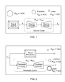
- FIG. 1 depicts a conventional source coding system
- FIG. 2 depicts a processor coding system in accordance with an embodiment of the invention
- FIG. 3 depicts an embodiment of an intelligent system in accordance with the present invention
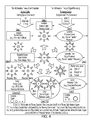
- FIG. 4 depicts the duality of elements between the two complementary pillars of Compression-Designs.
- FIG. 5 illustrates a block diagram of a KA-AMTI radar system
- FIG. 6 illustrates an embodiment of a Space-Time Processor in accordance with the present invention
- FIG. 7 is a SAR image of the Mojave Airport, California
- FIG. 8 is the image of FIG. 7 averaged to yield 64 range bins
- FIG. 9 is plot of front clutter to noise ratio
- FIG. 10 depicts the structure of a radar-blind clutter coder in accordance with the present invention.
- FIG. 11 depicts the structure of a radar-seeing clutter coder in accordance with the present invention.
- FIG. 12 is a clutter cell centroid plot of the range bins depicted in FIG. 8 ;
- FIG. 13 is an embodiment of a clutter covariance processor component in accordance with the present invention.
- FIGS. 14 a - 14 d illustrate the simulation results for range bin # 1 of FIG. 8 ;
- FIG. 15 depicts the antenna pattern of FIG. 5 in more detail
- FIGS. 16 a - 16 b depicts plots of the average and maximum SINR versus the range bins of FIG. 8 ;
- FIG. 17 depicts a 512 byte radar-blind PT decompressed SAR image
- FIG. 18 illustrates the RBCC clutter average power for range bin 1 plotted versus clutter cell number
- FIG. 19 illustrates the average SINR error for all 64 range bins
- FIG. 20 illustrates the average SINR error versus range bin number for the radar seeing case
- FIG. 21 illustrates the average SINR error versus range bin number for the radar blind case
- FIG. 22 is a plot of SMI-AASE as a function of the ratio of SMI samples
- FIG. 23 is a block diagram of a PT source coder architecture
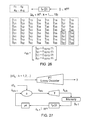
- FIG. 24 is a block diagram of a lossy PT encoder
- FIG. 25 is an illustration of transform pre-processing
- FIG. 26 is an illustration of predictive pre-processing
- FIG. 27 is a block diagram of a lossy PT decoder
- FIG. 28 is a block diagram of a lossless PT encoder
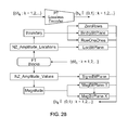
- FIG. 29 is an illustration of PT block decomposition
- FIG. 30 is an illustration of amplitude location decomposition
- FIG. 31 is an illustration of boundary decomposition
- FIG. 32 is an illustration of amplitude decomposition
- FIG. 33 is an illustration of magnitude decomposition
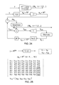
- FIG. 34 is a block diagram of a lossless PT decoder
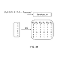
- FIG. 35 is an illustration of zero rows construction
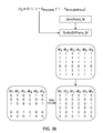
- FIG. 36 is an illustration of boundary bit plane construction
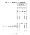
- FIG. 37 is an illustration of row ones construction
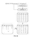
- FIG. 38 is an illustration of bit plane construction
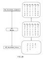
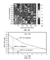
- FIG. 39 is an illustration of a 512 byte JPEG2000 decompressed SAR image
- FIG. 40 is an illustration of SMI-AASE versus Lmsi/NM.
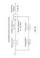
- FIG. 41 is a block diagram of an embodiment of the space-time sidelobe canceller structure for an antenna-based radar application according to the present invention.
- FIG. 1 a source coding system is shown where the output of the signal source is a discrete random variable X whose possible realizations belong to a finite alphabet of L elements, i.e., X ⁇ a 1 , . . . , a L ⁇ . Furthermore, the amount of “information” associated with the appearance of the element a i on the output of the signal source is denoted as I(a i ) and is defined in terms of the probability of a i , p(a i ), as follows:
- the signal source rate (in bits/sample) is defined by R ss and is usually significantly greater than the source entropy H(X) as indicated in FIG. 1 .
- a source coder is presented which is made up of an encoder followed by a decoder section. The input of the source coder is the output of the signal source, while its output is an estimate ⁇ circumflex over (X) ⁇ of its input X.
- the source coder rate is defined as R sc and is generally smaller than the signal source rate R ss .
- time duals of bits, information, entropy, and a source coder in source coding are bors, latency, ectropy and a processor coder in processor coding, respectively.
- “Latency” is the minimum time delay from the input to a specified scalar output of the signal processor that can be derived from redesigning the internal structure of the signal processor subjected to implementation components and architectural constraints;
- Processor coder is the efficient signal processor that is derived using the processor coding methodology.
- a processor coder like a source coder can be either lossless or lossy depending whether its output matches the original signal processor output.
- G ⁇ ( y ) max L ⁇ ( y i ) ⁇ [ L ⁇ ( y 1 ) , ... ⁇ , L ⁇ ( y M ) ] ( 1.3 )
- the signal processor rate (in bors/y) is R SP and is normally significantly greater than the processor ectropy G(y) as indicated in FIG. 2 .
- a processor coder is presented that is made up of an encoder followed by a decoder section.
- the input of the processor coder x is the same as the input of the signal processor while its output is an estimate ⁇ of the signal processor output y.
- the processor coder rate is R PC and is smaller than the signal processor rate R SP .
- the compression-designs or Conde methodology according to the present invention have been applied to a simulation of a real-world intelligent system problem with remarkable success. More specifically, the methodology has been applied to the design of a simulated efficient intelligent system for knowledge aided (KA) airborne moving target indicator (AMTI) radar that is subjected to severely taxing environmental disturbances.
- the studied intelligent system includes clutter in the form of SAR imagery used as the intelligence or prior knowledge and a clutter covariance processor (CCP) used as the intelligence processor.
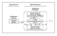
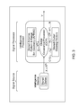
- FIG. 3 the basic structure of the intelligent system is shown and includes a storage device for the clutter and the intelligence processor containing a clutter covariance processor receiving external inputs from the storage device as well as internal inputs.
- the internal inputs of the CCP are the antenna pattern and range bin geometry (APRBG) of the radar system and the complex clutter steering vectors.
- ARBG antenna pattern and range bin geometry
- This intelligent system is responsible for the high signal to interference plus noise ratio (SINR) radar performance achieved with KA-AMTI but requires prohibitively expensive storage and computational requirements.
- the source coder that replaces the clutter source should be designed with knowledge of the radar system APRBG: In other words the source coder is radar seeing. This result yields a compression ratio of 8,192 for the tested 4 MB SAR imagery but has the drawback of requiring knowledge about the radar system before the compression of the SAR image is made.
- the source coder that replaces the clutter source can be designed without knowledge of the APRBG and is therefore said to be radar blind. This result yields the same compression ratio of 8,192 as the radar seeing case but is preferred since it is significantly simpler to implement and can be used with any type of radar system.
- FIG. 4 is a diagrammatic summary of the previously presented observations regarding certain characteristics of compression designs.
- FIG. 4 includes two columns. In the left column, space compression source coding is highlighted, while on the right column, time compression processor coding is illustrated. Nine different cases are displayed in this image.
- CASE 0 appearing in the middle of the figure, displays the signal source and signal processor for which one wishes to compress space and time, respectively.
- the picture in the middle between the signal source and the signal processor is composed of three major parts, which are described as follows:
- the sun triangles consisting of eight different triangles, each represent a different application where the signal source and signal processor may be used.
- the intensity of the shading inside these triangles denotes the application performance achieved in each case. Note that on the lower right hand side of the figure a chart is given setting forth the triangle appearance and corresponding application performance level.
- the darkest shading is used when an application achieves an optimum performance, whether or not the considered signal source and signal processor are compressed. Clearly the application's performance is optimum and therefore the shading is darkest for the lossless signal source and signal processor of CASE 0 ;
- the large gray colored circle without a highlighted boundary represents the amount of memory space required to store the signal output of the signal source.
- On the left and bottom part of the image it is shown how the diameter of the gray colored circle decreases as the required memory space decreases.
- Two cases are displayed. One case corresponds to the lossless case and the other case corresponds to the lossy case.
- the lossy case in turn can be processor blind or processor seeing which displays an opening in the middle of the gray circle. Also, it should be noted that for the processor blind case the boundary of the gray circle is not smooth;
- An unfilled black circle represents processor speed, where the reciprocal of its diameter reflects the time taken by the signal processor to produce an output. In other words the larger the diameter the faster the processor.
- CASE 1 displays a “lossless” source coder using the signal processor of CASE 0 where it is noted that the only difference between the illustrations for CASE 0 and CASE 1 is in the diameter of the space compression gray circle that is now smaller.
- CASE 2 is the opposite of CASE 1 where the diameter of the time compression unfilled black circle is now larger since the “lossless” processor coder is faster.
- CASE 3 combines CASES 1 and 2 resulting in an optimum solution in all respects, except it may still be taxing in terms of memory space and computational time requirements.
- CASES 4 thru 8 are “lossy” cases.
- CASES 4 and 5 pertain to either processor blind or processor seeing source coder cases where it is noted that the fundamental difference between the two is that the processor blind case yields a very poor application performance. On the other hand, the performance of the processor seeing case is suboptimum but very close to the optimum one.
- CASE 6 addresses the “lossy” processor coder case in the presence of a “lossless” source coder. For this case, everything seems to be satisfactory except that the required memory of the lossless source coder may still be too large.
- CASES 7 and 8 present what occurs when the two types of lossy source coders are used together with a ‘lossy’ processor coder. For these two cases it is found that the application performance is outstanding. CASE 7 , in particular, is truly remarkable since it was found earlier for CASE 4 that a radar-blind source coder yields a very poor application performance when the processor coder is ‘lossless’. Thus it is concluded that CASE 7 is preferred over all other cases since while achieving an outstanding application performance it is characterized by excellent space and time compressions.
- the time compression processor coding methodology gives rise to an exceedingly fast clutter covariance processor compressor (CCPC).
- the CCPC includes a look up memory containing a very small number of predicted clutter covariances (PCCs) that are suitably designed off-line (e.g., in advance) using a discrete number of clutter to noise ratios (CNRs) and shifted antenna patterns (SAPs), where the SAPs are mathematical computational artifices not physically implemented.
- CNRs clutter to noise ratios
- SAPs shifted antenna patterns
- the CCPC embodying the present invention is both very fast and yields outstanding SINR radar performance using SAR imagery which is either radar-blind or radar-seeing and has been compressed by a factor of 8,192.
- the radar-blind SAR imagery compression results are truly remarkable in view of the fact that these simple and universal space compressor source coders cannot be used with a conventional CCP.
- the advanced CCPC is a ‘lossy’ processor coder that inherently arises from a novel practical and theoretical foundation for signal processing, namely, processor coding, that is the time compression signal processing dual of space compression source coding.
- the coding concepts include bor (or time delay needed for the execution of some specified binary operator), latency (or minimum time delay required to generate a scalar output for a signal processor after the internal structure of the signal processor has been redesigned subject to implementation components and architectural constraints), and ectropy (or maximum latency among all the latencies derived for the signal processor scalar outputs), respectively.
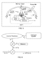
- FIG. 5 depicts an overview of a KA-AMTI radar system. It includes two major structures. They are: 1) An iso-range ring, or range bin, for a uniform linear array (ULA) in uniform constant-velocity motion relative to the ground. Only the front of the iso-range ring is shown, corresponding to angle displacements from ⁇ 90° to 90° relative to the antenna array boresight; and 2) An AMTI radar composed of an antenna, a space-time processor (STP) and a detection device.
- STP space-time processor
- KA-AMTI clutter returns are available in the form of SAR imagery that is obtained from a prior viewing of the area of interest. From this figure it is also noticed that the range bin is decomposed into NC clutter cells.
- NC is often greater than or equal to NM, where N is the number of antenna elements and M is the number of transmitted antenna pulses during a coherent pulse interval (CPI).
- CPI coherent pulse interval
- Table 1 is a summary of the relevant parameters, including those for M and N.
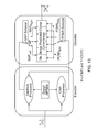
- FIG. 6 illustrates an embodiment of the STP architecture in accordance with the present invention. This input to the system is the addition of two signals, x and s. They are:
- ⁇ t is the angle of attack (AoA) of the target with respect to boresight; b) d is the antenna inter-element spacing; c) ⁇ is the operating wavelength; d) ⁇ t is the normalized ⁇ t ; e) T r is the pulse repetition interval (PRI); f) f r is the pulse repetition frequency (PRF); g) v t is the target radial velocity; h) f D t is the Doppler of the target; and i) f t D is the normalized f D t .
- NM ⁇ 1 dimensional vector x representing all system disturbances, which include the incident clutter, jammer, channel mismatch (CM), internal clutter motion (ICM), range walk (RW), antenna array misalignment (AAM), and thermal white noise (WN).
- CM channel mismatch
- ICM internal clutter motion
- RW range walk
- AAM antenna array misalignment
- WN thermal white noise
- SINR signal to interference plus noise ratio
- R n , R c f , R c b , R C , R J , R RW , R ICM and R CM are covariance matrices of dimension NM ⁇ NM and the symbol O denotes a Hadamard product or element by element multiplication.
- these disturbance covariances correspond to: R n (thermal white noise); R c f (front clutter); R c b (back clutter); R C (total clutter); R J (jammer); R RW (range walk); R ICM (internal clutter motion); and R CM (channel mismatch).
- the covariances R RW , R ICM and R CM are referred to as CMTs.
- the covariances R n and R c f are repeatedly used herein, and they are described as follows:
- ⁇ n 2 is the average power of thermal white noise and I NM is an identity matrix of dimension NM ⁇ NM. Notice from Table 1, in the examples presented herein, this noise power is assumed to be 1.
- R c f is the output of the intelligent system of FIG. 6 and is described as follows:
- the index i refers to the i-th front clutter cell on the range bin section shown on FIG. 5 ; b) ⁇ c i is the AoA of the i-th clutter cell; c) ⁇ AAM is the antenna array misalignment angle; d) f ⁇ c,i 2 is the i-th front clutter source cell power (excluding the antenna gain); e) G A f ( ⁇ c i , ⁇ t ) is the antenna pattern gain associated with the i-th front clutter cell; f) K f is the front global antenna gain; g) p c f ( ⁇ c i , ⁇ t ) is the “total” i-th front clutter cell power.
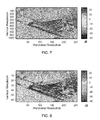
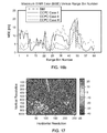
- the 4 MB 1,024 by 254 samples SAR image of the Mojave Airport in California ( FIG. 7 ) will be used with groups of sixteen consecutive rows averaged to yield the 64 range bins, as depicted in FIG. 8 .
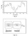
- FIG. 9 a plot is also given of the front clutter to noise ratio (CNR f ), i.e.,
- ⁇ n 2 1
- c f ( ⁇ c i , ⁇ AAM ) is the NM ⁇ 1 dimensional and complex i-th clutter cell steering vector
- i) v p is the radar platform speed
- j) ⁇ c ⁇ i is the normalized ⁇ c i
- k) ⁇ is the ratio of the distance traversed by the radar platform during the PRI, v p T r , to the half antenna inter-element distance, d/2.
- expressions (2.14)-(2.15) define the clutter covariance processor or intelligence processor of the intelligent system of FIG. 3 .
- the front clutter source cell power is the output of the intelligence source that the intelligence processor operates on.
- ⁇ c i is the AoA of the i-th back clutter cell
- c) b ⁇ c,i 2 is the i-th back clutter source cell power (assumed one for all i; see Table 1, entry b);
- G A b ( ⁇ c i , ⁇ t ) is the back antenna pattern gain associated with b ⁇ c,i 2 ;
- K b is the global back antenna gain (assumed 10 ⁇ 4 , see Table 1, entry a);
- p c b ( ⁇ c i , ⁇ t ) is the total clutter cell power of the i-th back clutter cell (the back clutter to noise ratio, CNR b , is described as:
- Jammer The jammer covariance R J is given by
- R RW space 1 N ⁇ N (2.42)
- a) c is the velocity of light
- b) B is the bandwidth of the compressed pulse
- c) ⁇ R is the range-bin radial width
- d) ⁇ is the mainbeam width
- e) A is the area of coverage on the range bin associated with ⁇ at the beginning of the range walk
- f) ⁇ A is the remnants of area A after the range bin migrates during a CPI; and
- ICM CMT Internal Clutter Motion
- f c is the carrier frequency in megahertz
- b) ⁇ is the wind speed in miles per hour
- c) r is the ratio between the dc and ac terms of the clutter Doppler power spectral density
- d) b is a shape factor that has been tabulated
- e) c is
- CM CMT R CM
- R NB R NB O R FB O R AD (2.48) where R NB , R FB and R AD are composite CMTs, as described below.
- Angle Independent Narrowband R NB is an angle-independent narrowband or NB channel mismatch CMT, which is described as follows:
- Finite Bandwidth R FB is a finite (nonzero) bandwidth or FB channel mismatch CMT, which is described as follows:
- R FB R FB time ⁇ R FB space ( 2.53 )
- R FB time 1 M ⁇ M ( 2.54 )
- [ R FB space ] i , k ( 1 - ⁇ / 2 ) 2 ⁇ sin ⁇ ⁇ c 2 ⁇ ( ⁇ / 2 ) ⁇ ⁇ for ⁇ ⁇ i ⁇ k ( 2.55 )
- ⁇ and ⁇ denote the peak deviations of decorrelating random amplitude and phase channel mismatch, respectively.
- Angle Dependent R AD is a reasonably approximate angle-independent CMT for angle-dependent or AD channel mismatch, which is described as follows:
- R AD R AD time ⁇ R AD space ( 2.57 )
- R AD time 1 M ⁇ M ( 2.58 )
- R AD space ] i , k sin ⁇ ⁇ c ⁇ ( B ⁇ ⁇ k - i ⁇ ⁇ d c ⁇ sin ⁇ ⁇ ( ⁇ ) ) ⁇ ⁇ for ⁇ ⁇ i ⁇ k ( 2.59 )
- [ R AD space ] i , i 1 ( 2.60 )
- Two general approaches can be used to derive R. They are:
- X i denotes radar measurements from range bins close to the range bin under investigation
- Lsmi is the number of measurement samples
- ⁇ 2 diag I is a diagonal loading term.
- FIG. 3 presents the intelligence source and intelligence processor subsystems of the intelligent system of FIG. 6 .
- the intelligence source contains the stored SAR imagery or clutter, while the intelligence-processor or CCP uses as its external input the output of the SAR imagery source, and as internal inputs the antenna pattern and range bin geometry or APRBG and the front clutter steering vectors (2.18) to compute the front clutter covariance matrix (2.15).
- APRBG antenna pattern and range bin geometry
- APRBG the front clutter steering vectors
- FIG. 10 illustrates the basic structure of a radar-blind clutter coder (RBCC), which includes an intelligence source coder containing the compressed or encoded clutter where the APRBG was not used.
- RBCC radar-blind clutter coder
- a clutter decompressor is included to derive an estimate for the uncompressed clutter for use by the conventional CCP or intelligence processor.
- the combination of the RBCC and conventional CCP is denoted here as RBCC-CCP for short. It has been found that this simple scheme generally does not produce a satisfactory SINR radar performance with reasonable compression ratios for SAR imagery.
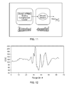
- FIG. 11 depicts the radar-seeing clutter coder (RSCC) structure, where the only difference from that of the radar-blind case of FIG. 10 is that the source-coder makes use of the APRBG.
- RSCC-CCP radar-seeing clutter coder
- the combination of the RSCC and a conventional CCP is denoted as RSCC-CCP for short. It has been found that outstanding SINR radar performance is derived when SAR imagery is compressed from 4 MB to 512 bytes for a compression ratio of 8,192.
- the RSCC scheme requires that minimum and maximum CNR values be found for the SAR image when processed in any direction. In the example presented herein, 41 and 75 dB were used for these values, respectively, which are also noted to be in accord with the CNR plot of FIG. 9 .
- the front clutter source cell power f ⁇ c,i 2 was generally in the range between 0.0077 and 7.7 which correspond to the minimum and maximum CNR values of 41 and 75 dB, respectively, as well as the assumed front global antenna gain given in Table 1.
- the resultant power limited SAR image was then compressed using standard compression schemes, e.g., PT source-coding.
- FIG. 17 a 512 byte radar-seeing PT decompressed SAR image is shown for a compression ratio of 8,192.
- FIG. 20 the corresponding average SINR error is given for the 64 range-bins of FIG. 8 . Note that this figure is characterized by a very small AASE value of approximately 0.7 dB.
- FIG. 20 and FIG. 21 reveals that the radar-seeing scheme achieves much better SINR radar performance for the same amount of compression. However, it should be kept in mind, that this improvement is achieved at the expense of the prerequisite prior knowledge of the APRBG.
- the clutter covariance processor compressor (CCPC) embodying the present invention achieves significant “on-line” (i.e., real time) computational time compression over the conventional clutter covariance processor or CCP. Simulations have shown that the CCPC is in fact the time compression dual of a space compression “lossy” source coder.
- the CCPC according to the present invention is eminently lossy since its output does not need to emulate that of the straight CCP. This is the case since its stated objective is to derive outstanding SINR radar performance regardless of how well its output compares with that of the local intelligence processor.
- the shape of the range bin cell power is a function of the antenna pattern G A f ( ⁇ c i , ⁇ t ) as well as the front clutter source cell power f ⁇ c,i 2 which often varies drastically from range bin to range bin.
- the variation of the clutter source cell power f ⁇ c,i 2 from range bin to range bin is the source of the on-line computational burden associated with (2.14)-(2.15) since otherwise these expressions could have been solved off-line.
- the on-line computational time delay problem of the conventional CCP is addressed in two steps, where each step has two parts.
- K j for all j are real constants that are determined on-line for each range bin using as a basis the measured input waveform ⁇ f ⁇ c,i 2 ⁇ . Since a desirable result is to achieve the smallest possible “on-line” computational time delay while yielding a satisfactory SINR radar performance, a single constant, K 0 , has been selected to model the entire clutter source cell power waveform.
- the numerical value for K 0 is determined such that it reflects the strength of the clutter.
- the strength of the clutter is related to the front clutter to noise ratio or CNR f defined earlier in (2.24) and plotted in FIG. 9 for the 64 range bins of FIG. 8 .
- the CNR f will be one of two real and scalar values derived by the CCPC where it is assumed that the thermal white noise variance ⁇ n 2 is 1.
- Step I a suitable modulation of the antenna pattern waveform ⁇ G A f ( ⁇ c i , ⁇ t ⁇ is sought.
- the modulation of this internal CCP input can be achieved in several ways. Two of them are: a) By using peak-modulation which consists of shifting the peak of the antenna pattern to some direction away from the target; and b) By using antenna elements-modulation which consists of widening or narrowing the antenna pattern mainbeam by modifying the number of “assumed” antenna elements N. It is emphasized here that these are only a mathematical alteration of the antenna pattern, since the true antenna pattern remains unaffected.
- Peak-modulation may be selected since, as mentioned earlier, the main objective is to achieve the smallest possible “on-line” computational delay for the computational time compressed CCP. Furthermore, to find the position to where the peak of the antenna pattern should be shifted to, the clutter cell centroid (CCC) or center of mass of the clutter is evaluated for each range bin.
- the CCC is the second of two scalar values derived by the CCPC and is given by the following expression
- FIG. 12 the CCC plot is shown for the 64 range bins of the SAR image given in FIG. 8 . It should be noted that for many of the 64 range bins the CCC varies significantly from the position of the assumed target at 128.5 (0° from boresight). Clearly, for the isotropic clutter case the CCC will reside at boresight.
- Step II In this first part of Step II a finite and fixed number of predicted clutter covariances or PCCs are found off-line. This is accomplished using the CCP describing equations (2.14)-(2.15) subject to the simple clutter model (3.1) and a modulated antenna pattern which results in a small and fixed number of highly lossy clutter covariance realizations.
- the PCCs are derived from the following expressions:
- the CCPC includes CNR and CCC processors where their input is given by the waveform ⁇ f X ⁇ c,i 2 ⁇ and f X ⁇ c,i 2 denotes the i-th front clutter source cell power corresponding to three different cases for X, which are as follows:
- X UCMD when the clutter emanates from the storage uncompressed clutter memory device (UCMD) of FIG. 3 .
- X RBCC when the clutter is generated from the radar-blind clutter coder of FIG. 10 .
- X RSCC when the clutter is derived from the radar-seeing clutter coder of FIG. 11 .
- the CCPC selects from the memory containing the 6 PCCs of FIG. 13 the one that is better matched to the measured CCC and CNR processor output values. For instance, if the CCC processor output is 140 , the selection process is narrowed down to the pair of PCCs that were evaluated using the SAP that is shifted to position 139 on the range bin (or +7°), since it is the closest. In addition, if the measured CNR processor output is 60 dB the element of the selected PCC pair associated with the 75 dB PCNR is selected. It should be noted that the PCNRj selected is the one “above” the measured CNR processor output value.
- the Centroid and CNR Processors of FIG. 13 govern the time delay associated with the CCPC, and thus constitute a ‘lossy processor encoder’ since they encode in a lossy fashion the time delay essence, i.e., the ectropy, of the original CCP.
- the second observation is that the look up memory section of FIG. 13 is a ‘lossy processor decoder’ since it reconstructs a highly lossy version of the output of the original CCP.
- CCPC UCMD is the total disturbance covariance (2.11)-(2.12) with the CCPC output of FIG. 13 , CCPC UCMD R c f , replacing the front clutter covariance matrix R c f in (2.12); and b) S CCPC UCMD is the set of UCMD and CCPC parameters that define the specific CCPC case.
- This second CCPC Case II has three PCC pairs. One is associated with the antenna pattern of FIG. 5 and the other two with two different SAPs.
- This third CCPC Case III has five PCC pairs. One is associated with the antenna pattern of FIG. 5 and the other four with four different SAPs.
- w [ smi ⁇ R ] - 1 ⁇ s ( 3.12 )
- X i denotes radar measurements from range bins close to the range bin under investigation
- Lsmi is the number of measurement samples
- ⁇ 2 diag I is a diagonal loading term.
- FIGS. 14 a - 14 d are now explained in some detail.
- the ideal front clutter average power p c f ( ⁇ c i , ⁇ t ) of (2.15) is plotted versus the range bin cell position.
- range bin cell position 1 corresponds to ⁇ 90°, 128.5 to 0° and 256 to +90° where all the angles are measured from boresight.
- the average power axis has been marked with the corresponding CNR of 59 dB and the cell position axis with the corresponding CCC of 104.1 which is also noted to reside 24.4 range bin cells away ( ⁇ 17.1°) from the assumed target location of 128.5 or 0°.
- the ideal clutter waveform is then contrasted with the predicted ones derived from (3.4) and linked to the selected PCC for each CCPC scheme.
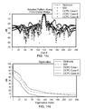
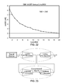
- FIG. 22 is a plot of SMI-AASE as a function of the ratio of SMI samples, Lsmi, over the number of STAP degrees of freedom NM. From this figure it is noted that this ratio must be equal to 20 (corresponding to 5,120 SMI samples), to achieve an AASE value of 3 dB which is, at least, a factor of 10 larger than that required if the SAR image had been of a homogeneous terrain. From this figure it is concluded that the derived SINR radar performance is not satisfactory for the SMI algorithm.
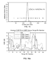
- FIG. 14 a the legend “Pred Clutter I (8, 75.0 dB)” pertains to the front predicted clutter average power (3.4) for CCPC Case I.
- this figure is characterized by the following set of zero crossings and mainlobe peak positions across the range-bin:
- This set is then used to denote the possible directions to which the true antenna pattern of FIG. 5 can be shifted.
- these possible directions are those given in expressions (3.9)-(3.11) where SAPs are defined for three different CCPC cases. These directions can generally be anywhere in the specified range of cell locations from 1 to 256. In fact, numerous simulations have revealed outstanding SINR radar performance with directions that are anywhere in between the best two adjacent directions selected from (3.15). In other words, these directions have only been selected because they scan the entire range bin from cell 1 to cell 256 and have some connection to the lobes of the true antenna pattern.
- the ordered pairs appearing in FIG. 14 a are explained as follows.
- the ordered pair (8, 75.0 dB) next to the title Pred Clutter I indicate that the SAP associated with the selected PCC of CCPC Case I of (3.9) is the physically implemented antenna pattern of FIG. 15 where the predicted clutter to noise ratio or PCNR is 75.0 dB.
- the legend Pred Clutter II (7, 75.0 dBs) indicates that the plotted predicted clutter covariance power waveform corresponds to that of CCPC Case II of (3.10) where the antenna pattern had been shifted to ⁇ 7° away from boresight and the PCNR is once again 75.0 dB.
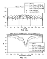
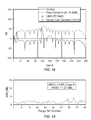
- FIG. 14 b the SINR results derived with each scheme are presented.
- the title for each legend is self explanatory, and the ordered pairs each indicate the maximum SINR error followed by the average SINR error.
- significantly better results are derived for CCPC Cases II and III than the SMI case and the CCPC Case I.
- CCPC Case III outperforms CCPC Case II by a relatively small amount.
- FIG. 14 c the adapted pattern corresponding to all contrasted cases is plotted.
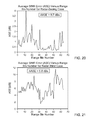
- FIGS. 16 a and 16 b the average and maximum SINR errors are plotted versus the 64 range bins of FIG. 8 .
- the results presented in FIGS. 16 a and 16 b correlate with those presented for range bin # 1 .
- CCPC Cases II and III (with average of average SINR error (AASE) values of 1.2 and 1.16, respectively) yield a satisfactory SINR performance while the SMI and CCPC Case I do not.
- the RBCC is of the predictive-transform type and compresses the SAR image from 4 MB to 512 bytes. In FIG. 17 the corresponding 512 byte radar-blind PT decompressed SAR image is shown.
- FIG. 17 a 512 bytes radar-blind PT decompressed SAR image is shown. It should be noted that the amount of compression is very significant, i.e., a factor of 8,192, since the original SAR image was compressed from 4 MB to 512 bytes.
- This PT technique outperforms in signal to noise ratio (SNR) wavelets based JPEG2000 by more than 5 dBs.
- SNR signal to noise ratio
- FIG. 21 the corresponding average SINR error for all 64 range bins is presented An inspection of FIG. 21 reveals an AASE value of 5.8 dB which is unsatisfactory for a KA type technique.
- this radar-blind technique becomes much more useful when the covariance processor of expressions (2.14)-(2.15) is replaced with a new type of covariance processor, a type that is derived using a novel processor coding methodology, which is the time compression dual of space compression source coding.
- a radar-seeing technique is next considered that yields significantly better results than that derived with the radar-blind technique but that requires knowledge of the antenna pattern and range bin geometry or APRBG.
- the RBCC clutter average power is plotted versus clutter cell number, as well as the associated predicted clutter average power for CCPC Case III.
- the average SINR error is presented versus all the 64 range bins where the AASE is given by 1.27 dB. It was found that when the conventional CCP was implemented with the RBCC scheme it yielded an AASE value of 5.8 dBs.
- the examples presented in accordance with the present invention demonstrate that a SAR imagery clutter covariance processor appearing in KA-AMTI radar can be replaced with a fast clutter covariance processor resulting in outstanding SINR radar performance while processing clutter that had been highly compressed using a predictive-transform radar-blind scheme.
- the advanced fast covariance processor is a lossy processor coder that inherently arises as the time compression processor coding dual of space compression source coding. Since a more complex radar-seeing scheme generally did not significantly improve the results obtained with the radar-blind case, the radar-blind clutter compression method is preferred due to its simplicity and universal use with any type of radar system.
- a fundamental problem in source coding is to provide a replacement for the signal source, called a source coder, characterized by a rate that emulates the signal source entropy.
- This type of source coder is lossless since its output is the same as that of the signal source such as is the case with Huffman, Entropy, and Arithmetic coders.
- Another fundamental problem in source coding pertains to the design of lossy source coders that achieve rates that are significantly smaller than the signal source entropy.
- Lossy PT source coding is a source coding technique that is derived by combining predictive source coding with transform source coding using a minimum mean squared error (MMSE) criterion subjected to appropriate implementation constraints.
- MMSE minimum mean squared error
- a byproduct of this unifying source coding formulation is coupled Wiener-Hopf and eigensystem equations that yield the prerequisite prediction and transformation matrices for the PT source coder.
- the basic idea behind the PT source coder architecture is to trade off the implementation simplicity of a sequential predictive coder with the high speed of a non-sequential transform coder.
- Simplified decomposed PT structures are noted to arise when signals are symmetrically processed.
- a strip processor is an example of such processing.
- cascaded Hadamard structures are integrated with PT structures to accelerate the on-line evaluation of the necessary products between a transform or predictor matrix and a signal vector.
- the excellent space compression achieved with lossy PT source coding is not affected by its integration with a very fast and simple bit planes methodology that operates on the quantized coefficient errors emanating from the PT encoder section.
- the efficacy of the methodology will be illustrated by compressing SAR imagery of KA-AMTI radar that is subjected to severely taxing environmental disturbances.
- PT source coding with bit planes significantly outperforms wavelets based JPEG2000 in terms of local SNR as well as global SINR radar performance.
- the overall PT source coder architecture is shown. It has as its input the output of a signal source y. As an illustration, this output will be assumed to be a real matrix representing 2-D images.
- the structure includes two distinct sections. In the upper section, the lossy encoder and associated lossy decoder are depicted while in the lower section the lossless encoder and decoder are shown. Before the lossless section of the coder is explained, which contains the offered bit planes, the lossy section will be reviewed.
- FIG. 24 the lossy PT encoder structure is shown. It includes a transform pre-processor f T (y) whose output x k is a real n dimensional column vector. In FIG.
- the pixel vector x k then becomes the input of an n ⁇ n dimensional unitary transform matrix T.
- the multiplication of the transform matrix T by the pixel vector x k produces an n dimensional real valued coefficient column vector c k . This coefficient, in turn, is predicted by a real n dimensional vector ⁇ k/k ⁇ 1 .
- the prediction vector ⁇ k/k ⁇ 1 is derived by multiplying the real m dimensional output z k ⁇ 1 of a predictor pre-processor (constructed using previously encoded pixel vectors, as discussed below), by a m ⁇ n dimensional real prediction matrix P. A real n dimensional coefficient error ⁇ c k is then formed and subsequently quantized yielding ⁇ k .
- the quantizer has two assumed structures. One is an “analog” structure that is used to derive analytical design expressions for the P and T matrices and another is a “digital” structure used in actual compression applications. The analog structure allows the most energetic elements of ⁇ c k to pass to the quantizer output unaffected and the remaining elements to appear at the quantizer output as zero values, i.e.,
- the quantizer output ⁇ k is then added to the prediction coefficient ⁇ k/k ⁇ 1 to yield a coefficient estimate ⁇ k/k .
- the quantizer used here (4.2) is simple to implement and yields outstanding results.
- the coefficient estimate ⁇ k/k is then multiplied by the transformation matrix T to yield the pixel vector estimate ⁇ circumflex over (x) ⁇ k/k .
- This estimate is then stored in a memory which contains the last available estimate ⁇ k ⁇ 1 of the pixel matrix y. It should be noted that the initial value for ⁇ k ⁇ 1 , i.e., ⁇ 0 , can be any reasonable estimate for each pixel.
- the initial ⁇ 0 can be constructed by assuming for each of its pixel estimates the average value of the pixel block x 1 .
- the design equations for the T and P matrices are derived by minimizing the mean squared error expression E[(x k ⁇ circumflex over (x) ⁇ k/k ) t (x k ⁇ circumflex over (x) ⁇ k/k )] (4.3) with respect to T and P and subject to three constraints. They are:
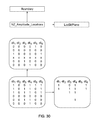
- FIG. 27 the lossy PT decoder is shown.
- the coefficient error sequence forms what is called in the figure PT Blocks which is a matrix of dimension n ⁇ N B .
- PT Blocks which is a matrix of dimension n ⁇ N B .
- N B 6.
- the most energetic element of each quantized coefficient error is found in the first row of PT Blocks, i.e., in the row ⁇ 3 0 0 ⁇ 1 1 2 ⁇ , and the least energetic one is found in the last row, i.e., the row ⁇ 0 0 0 ⁇ 1 0 0 ⁇ .
- NZ_Amplitude_Locations is an n ⁇ N B dimensional matrix that conveys information about the location of the nonzero (NZ) amplitudes found in PT Blocks. From the simple example of FIG. 29 , it is noted that all nonzero elements of PT Blocks are replaced with a 1. NZ_Amplitude_Values, on the other hand, retain the actual values of the nonzero amplitudes. In FIG. 29 , these amplitudes are shown for the example where it is noted that the number of elements in each row is not constant and also that no elements are displayed corresponding to the fourth row of PT Blocks since this row is made of zero values only.
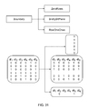
- the NZ_Amplitude_Locations matrix is now split up into a Boundary matrix and a LocBitPlane block.
- the Boundary matrix is associated with the location where the zero runs begin in the direction from top to bottom of each column of the NZ_Amplitude_Locations matrix.
- LocBitPlane are the bits that remain after the 1's followed by zero runs of the Boundary matrix are eliminated from the NZ_Amplitude_Locations matrix.
- this decomposition is illustrated for the running example.
- the Boundary matrix has three symbols. They are 0, 1 and X.
- the symbol X is used for the elements of a row whose values are all zero, and thus it informs about a zero row.
- the symbol 1 does not appear more than once for each column and specifies a boundary location where the zero run begins for that particular column. For example, since the zero run starts at row 4 for the first column, the 1 is placed on the third row just prior to the beginning of the zero run.
- the aforementioned LocBitPlane is also illustrated in FIG. 30 . It should be noted how for the third column only the bits ⁇ 0 1 1 ⁇ are listed and the zero for the fourth row is ignored since this information is available from the encoding of the Boundary matrix.
- the Boundary matrix is decomposed into three blocks. They are the blocks ZeroRows, BndryBitPlane and RowOneOnes. This decomposition is best explained with the illustrative example of FIG. 31 . From this figure it is noted that ZeroRows assigns a 0 to a row of the Boundary matrix if it is composed of the special symbol X, otherwise it assigns a 1 to the row. BndryBitPlane is the same as Boundary matrix except that all rows made up of the special symbol X are removed. In addition, BndryBitPlane replaces a 0 with a 1 in the first row of a column with a full zero run.
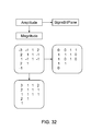
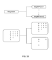
- NZ_Amplitude_Values is decomposed into two blocks. One is a Magnitude block and the other is a SignsBitPlane block. The nature of these two blocks is illustrated in FIG. 32 , where the SignsBitPlane block assigns a zero to a negative integer value and a one to a positive integer value. The Magnitude block is self explanatory. Returning to FIG. 28 it is noted that the Magnitude block is decomposed into X MagBitPlane blocks. Each of these component blocks are readily explained via the illustrative example of FIG. 33 .
- MagBitPlane- 1 is noted from FIG. 33 to assign a 1 to the integer of magnitude 1 and a 0 to the other cases.
- MagBitPlane- 2 ignores all integers with a magnitude of one, and assigns a 1 to the integers with a magnitude of 2 and a 0 to the remaining integers.
- a lossless encoder such as an Arithmetic encoder whose output is then sent to the lossless PT decoder.
- the lossless PT decoder which receives as input the output of the lossless PT encoder (note it is assumed here that a lossless decoder such as an Arithmetic decoder was appropriately used to derive this input).
- the front part of the decoder constructs an n ⁇ N B matrix, ZeroRows_M, made up of either unity rows or zero rows depending on the nature of the ZeroRows bits.
- FIG. 35 this construction is illustrated with the running illustrative example. Note that the ZeroRows bits that were derived in FIG. 31 are now used to construct a 6 ⁇ 6 matrix consisting of either unity or zero rows.
- the ZeroRows_M matrix is used in conjunction with the BndryBitPlane bits to generate the n ⁇ N B matrix BndryBitPlane_M. This process is illustrated in FIG. 36 .
- the next step is to use the derived BndryBitPlane_M matrix together with the RowOneOnes bits to derive a RowOneOnes_M matrix that is also of dimension n ⁇ N B . This process is illustrated in FIG. 37 .
- the RowOneOnes_M matrix is combined with the LocBitPlane bits to derived a LocBitPlane_M matrix of dimension n ⁇ N B . In FIG.
- the efficacy of the previously advanced bit planes PT method is now demonstrated by comparing it with wavelets based JPEG2000 in a real-world application.
- the application consists of compressing 4 MB SAR imagery by a factor of 8,192 and then using the decompressed imagery as the input to the covariance processor coder of a KA-AMTI radar system subjected to severely taxing environmental disturbances.
- This SAR imagery is prior knowledge used in KA-AMTI radar to achieve outstanding SINR radar performance.
- the 4 MB SAR image that will be tested is given in FIG. 7 .
- the magnitude of the image is in dBs and consists of 1024 rows and 256 columns, and represents an image of the Mojave Airport in California. This image was compressed using a 16 ⁇ 1 strip processor that moves on the image from left to right and top to bottom.
- FIG. 17 the decompressed SAR image is shown that was derived when the image was compressed by a factor of 8,192 using the PT source coder of this paper.
- the SINR radar performance derived with JPEG2000 is worse by 2 dB than that for the same PT source coding technique.
- the present invention relates to a simplified approach for determining the output of a total covariance signal processor.
- Such an approach may be used, for example, in connection with an antenna-based radar system to make a decision as to whether or not a target may be present at a particular location.
- estimating the output of a clutter covariance processor by performing certain calculations offline, characterizing the input signal using online calculations, and then using the online calculations to select one of the offline calculations, as discussed in the embodiments above dealing with clutter covariance processors
- a single offline set of calculations is performed and then used to estimate of the output of the total covariance processor in conjunction with the antenna signal obtained at the time of viewing a target.
- the antenna pattern is shifted to a Shifted Antenna Pattern (SAP) and the single set of offline calculations are performed with this SAP in mind.
- SAP Shifted Antenna Pattern
- the Shifted Antenna Pattern is determined based on some determination of the clutter centroid signal for the various range bins of the antenna image.
- the Shifted Antenna Pattern may be determined based on the standard deviation of the clutter centroid signal, or an RMS estimation of the clutter centroid signal.
- the SAP main lobe peak is restricted to reside at only one of the five positions specified in Equation 3.11 above.
- the offline determined best angle to shift the SAP to could be used to make the actual antenna pattern reflect this shifted position.
- a sample matrix inverse (SMI) technique can then be used with this SAP to yield a knowledge aided SMI scheme that can be viewed as an extreme case of memory space and computational time compressed KA-AMTI radar. Results for an application of such an approach are shown in FIG. 40 .
- the offline calculations may be performed for a single shifted antenna pattern, and this single set of offline calculations used in conjunction with the antenna signal obtained online to determine the estimated output of the clutter covariance processor.
- a simplified algorithm for performing matrix inversion is used, for example, in conjunction with the previously described embodiment where the output of the total covariance processor is estimated using an inverse matrix, such as the inverse matrix R ⁇ 1 discussed above.
- the simplified matrix inversion algorithm utilizes a sidelobe canceller approach for matrix inversion, in conjunction with the predictive transform estimation approaches discussed herein.
- the sidelobe canceller essentially removes and/or minimizes the effect of the antenna sidelobe signals on the antenna main beam return signal, x. Background information relating to sidelobe cancellers may be found in J. R. Guerci, Space - Time Adaptive Processing for Radar (Artech House, 2003), the contents of which are incorporated herein by reference.
- FIG. 41 therein is illustrated a block diagram of an embodiment of the space-time sidelobe canceller structure for an antenna-based radar application according to the present invention.
- the input to the sidelobe canceller is the output of the antenna, i.e., complex vector x of dimension NM.
- the antenna output x is also multiplied by a blocking (or null) matrix B(s) of dimension K ⁇ NM.
- E[x ij ] K (6.7)
- E [( x ij ⁇ K )( x i+v,j+h ⁇ K ) ( P avg ⁇ K 2 ) ⁇ D (6.8)
- ⁇ E [( x ij ⁇ K )( x i,j+1 ⁇ K )]/( P avg ⁇ K 2 ) (6.9)
- D ⁇ square root over (v 2 +h 2 ) ⁇ (6.10) where v and h are integers, is the average correlation coefficient between any two adjacent samples, K is the average value of any sample, and P avg is the average power associated with each sample.
- Equation 6.5 essentially functions to select the K-most energetic columns in the NM ⁇ NM covariance matrix, thereby resulting in a K ⁇ K matrix, which is then subject to the matrix inversion process.
- the matrix inversion is carried out on a relatively smaller K ⁇ K size matrix.
Abstract
Description
| TABLE 1 | ||
| a. | Antenna | N = 16, M = 16, d/λ = ½, fr = 103 Hz, fc = 109 Hz, |
| Kf = 4 × 10⁵ or 56 dBs, Kb = 10−4 or −40 dBs, | ||
| b. | Clutter | Nc = 256, β = 1, 41 dBs < 10log10CNRf < 75 dBs, |
| |
||
| c. | Target | θt = 0° |
| d. | Antenna Disturbance | σn 2 = 1, θAAM = 2° |
| e. | Jammers | NJ = 3, θJ |
| 10log10σJi 2 = 34 dBs for i = 1, 2, 3, 10log10JNR1 = 53 dBs, | ||
| 10log10JNR2 = −224 dBs and 10log10JNR3 = 66 dBs | ||
| f. | Range Walk | ρ = 0.999999 |
| g. | Internal Clutter Motion | b = 5.7, ω = 15 mph |
| h. | Narrowband CM | εi = 0 for all i, γi for all i fluctuates with a 5° rms |
| i. | Finite Bandwidth CM | Δε = 0.001, Δφ = 0.1° |
| j. | Angle Dependent CM | B = 108 Hz, Δθ = 28.6° |
| k. | Sample Matrix Inverse | Lsmi = 8 × 64 = 512, σdiag 2 = 10 |
w=R−1s (2.9)
SINR=w H ss H w/w H Rw (2.10)
R={R C O (R RW +R ICM +R CM)}+{R J O R CM }+R n (2.11)
R C =R c f +R c b (2.12)
Rn=σn 2INM (2.13)
where: a) the index i now refers to the i-th clutter cell on the back side of the iso-range ring, not shown in
and is assumed to be −40 dB, see Table 1, entry b); f) cb(θc i,θAAM) is the NM×1 dimensional and complex steering vector associated with bσc,i 2; and g) c 1(θc i) is as defined in (2.19)-(2.20).
Jammer
The jammer covariance RJ is given by
where: a) the index i refers to the i-th jammer on the range bin; b) NJ is the total number of jammers (assumed to be three; see Table 1, entry e); c) θJ i is the AoA of the i-th jammer (the location of the three assumed jammers are at −60°, −30°, and 45°; see Table 1, entry e); d)
is given by 53, −224, and 66 dB for the jammers at −60°, −30°, and 45°, respectively; see Table 1, entry e); and i) j(θJ i) is the NM×1 dimensional and complex i-th jammer steering vector that is noted from the defining equations (2.34)-(2.38) to be Doppler independent.
Range Walk
The range walk or RW CMT, RRW, is described as follows:
RRW=RRW time
[R RW time]i,k=ρ|i-k| (2.41)
R RW space=1N×N (2.42)
ρ=ΔA/A=ΔA/{ΔRΔθ}=ΔA/{(c/B)Δθ} (2.43)
where: a) c is the velocity of light; b) B is the bandwidth of the compressed pulse; c) ΔR is the range-bin radial width; d) Δθ is the mainbeam width; e) A is the area of coverage on the range bin associated with Δθ at the beginning of the range walk; f) ΔA is the remnants of area A after the range bin migrates during a CPI; and g) ρ is the fractional part of A that remains after the range walk (for example, ρ=0.999999; see Table 1, entry f).
Internal Clutter Motion
The internal clutter motion or ICM CMT, RICM, is described as follows:
where: a) fc is the carrier frequency in megahertz; b) ω is the wind speed in miles per hour; c) r is the ratio between the dc and ac terms of the clutter Doppler power spectral density; d) b is a shape factor that has been tabulated; and e) c is the speed of light. In the example presented herein, fc=1,000 MHz, ω=15 mph and b=5.7; see Table 1, entries a, g.
Channel Mismatch
The total channel mismatch or CM CMT, RCM, is described as follows:
RCM=RNBO RFBO RAD (2.48)
where RNB, RFB and RAD are composite CMTs, as described below.
Angle Independent Narrowband
RNB is an angle-independent narrowband or NB channel mismatch CMT, which is described as follows:
where in (2.52) Δε1, . . . , ΔεN and Δγ1, . . . , ΔγN denote amplitude and phase errors, respectively. In the example presented herein, the amplitude errors are assumed to be zero and the phase errors are assumed to fluctuate with a 5° root mean square (rms); see Table 1, entry h.
Finite Bandwidth
RFB is a finite (nonzero) bandwidth or FB channel mismatch CMT, which is described as follows:
where in (2.55)-(2.56) Δε and Δφ denote the peak deviations of decorrelating random amplitude and phase channel mismatch, respectively. In the example presented herein, Δε=0.001 and Δφ=0.1°; see Table 1, entry i.
Angle Dependent
RAD is a reasonably approximate angle-independent CMT for angle-dependent or AD channel mismatch, which is described as follows:
where B is the bandwidth of an ideal bandpass filter and Δθ is a suitable measure of mainbeam width. In the example presented herein, B=100 MHz and Δθ=28.6°; see Table 1, entry j.
Optimum Direct Inverse
The w that maximizes the SINR expression (2.10) is given by the following expression:
w=R−1s. (2.61)
Two general approaches can be used to derive R. They are:
where Xi denotes radar measurements from range bins close to the range bin under investigation, Lsmi is the number of measurement samples and σ2 diagI is a diagonal loading term. Xi may be derived via the following generating expression
X i =R i −1/2 x i (2.63)
where: a) xi is a zero mean, unity variance, NM dimensional complex random draw; and b) Ri is the total disturbance covariance (2.11)-(2.12) associated with the i-th range bin. In the example presented herein σdiag 2=10σn 2=10; see Table 1, entry k.
K0+K1i+K2i2+ . . . , (3.1)
where: a) ppc f (.) is the predicted front clutter power; b) GA f (θc i−θk,θt) is a shifted antenna pattern or SAP where the peak value of the actual antenna pattern (2.16) has been shifted from θc i=θt to θc i=θt+θk; c) θk denotes the amount of angular shift of the SAP away from the assumed target position θt (the SAPs are generally designed in pairs, one associated with θk and the other with −θk); d) NSAP is the number of SAPs considered (in the simulations the cases with N
In
where: a)
is the total disturbance covariance (2.11)-(2.12) with the CCPC output of
S CCPC UCMD={f σc,i 2,θ1=0°,PCNR1=57 dBs,PCNR2=75 dBs} (3.9)
S CCPC UCMD={f σc,i 2θ1=−7°,θ2=0°,θ3=7°,PCNR1=57 dBs,PCNR2=75 dBs} (3.10)
S CCPC UCMP={f σc,i 2,θ1=−14°,θ2=−7°,θ3=0°,θ4=7°,θ5=14°,PCNR1=57 dBs,PCNR2=75 dBs} (3.11)
where Xi denotes radar measurements from range bins close to the range bin under investigation, Lsmi is the number of measurement samples and σ2 diagI is a diagonal loading term. Xi was derived via the following generating equation
X i =R i −1/2 x i (3.14)
where: a) xi is a zero mean, unity variance, NM dimensional complex random draw; and b) Ri is the total disturbance covariance (2.11)-(2.12) associated with the i-th range bin. For the example presented herein, σdiag 2=10. For the results shown in
AP(θc i,θAAM,β,θt , f D t)=10 log10 |w H c f (θc i,θAAM)|2 (3.15)
where θAAM=2°, β=1, θt=0, f D t=0, In
AP(θc i,θAAM,β,θt ,f D t)=10 log10 |w H c f (θc i,θAAM)|2 (3.17)
where θAAM=2°, β=1, θt=0, f D t=0
δĉk =└gδc k+½┘ (4.2)
E[(xk−{circumflex over (x)}k/k)t(xk−{circumflex over (x)}k/k)] (4.3)
with respect to T and P and subject to three constraints. They are:
where these expressions are a function of the first and second order statistics of xk and zk−1 including their cross correlation. To find these statistics the following isotropic model for the pixels of y can be used:
E[yij]=K, (4.7)
E[(y ij −K)(y i+v,j+h −K)=(P avg −K 2)ρD (4.8)
ρ=E[(y ij −K)(y i,j+1 −K)]/(P avg −K 2)
D=√{square root over ((rv)2 +h 2)} (4.9)
where v and h are integers, K is the average value of any pixel, Pavg is the average power associated with each pixel, and r is a constant that reflects the relative distance between two adjacent vertical and two adjacent horizontal pixels (r=1 when the vertical and horizontal distances are the same).
y=x·w (5.1)
where x is based on the antenna signal, and w is a weighting vector determined online. In turn, w may be determined based on the following equations:
The SAP mainlobe peak position θshift was tested for the five cases in Equation 5.6 and the compressed/decompressed clutter source power f RBCCσc,i 2 was derived using a PT radar blind scheme. When these five processor coders were simulated with the radar blind clutter compressor or RBCC, the best AASE was produced when the SAP was shifted to either 14° or −14°. More specifically, the AASE values for these two cases emulated the value of 1.27 dBs for CCPC Case III discussed above. These results suggest that the simulated test SAR image is characterized by a pair of SAPs symmetrically placed with respect to the moving target or initial antenna position, and where only one of the Shifted Antenna Patterns is needed to yield satisfactory radar performance. An investigation of the clutter centroid information indicates that the direction to shift the antenna pattern to over all 64 range bins may be governed by some power of the standard deviation of the clutter centroid from the boresight position (CC=128.5). It is of interest to note that when the clutter is homogeneous, the clutter centroid will be equal to 128.5 for all 64 range bins and thus the selected SAP will point in the same direction as the actual unshifted antenna pattern as expected.
where: a) Xi(.) denotes a radar measurement from a range bin close to the range bin under investigation; b) Lsmi is the number of measurement samples; c) σ2 diagI is a diagonal loading term where σ2 diag=10; d) xi is a zero mean, unity variance, NM dimensional complex random draw; e) Ri is the total disturbance covariance associated with the ith range bin; and f) θshift is the angle from boresight to where the peak of the antenna pattern has been shifted.
w=(I−I+R −1)s (6.1)
wx=Isx−(I−R −1)sx (6.2)
where the term Isx corresponds to the main beam signal, and the term (I−R−1)sx corresponds to the sidelobe signal.
w 0 =[B(s)R B H(s)]−1 B(s)R s (6.3)
where R is the total covariance matrix. In turn, this multiplication yields the scalar complex sidelobe response
{circumflex over (d)} 0 =s H RB H(s)[B(s)RB H(s)]−1 B(s)x (6.4)
which is then subtracted from d0 to yield a scalar and complex beamformer residue z=d0−{circumflex over (d)}0 whose value is then used to determine if a target is present. The blocking matrix B(s) has K rows that are “approximately” orthogonal to s and given by the following expression
B(s)=[0K×1 I K 0K×(NM−K−1)][Diag(s)T PT]H (6.5)
where 0K×1 is a K dimensional column vector, IK is a K dimensional identity matrix, and 0K×1 is a K×(NM−K−1) dimensional zero matrix. Diag(s) is an NM dimensional diagonal matrix whose diagonal elements are the NM elements of s and TPT is a NM×NM predictive-transform (PT) matrix appropriately designed making use of the PT design equation and isotropic statistics set forth below.
PT Design Equation
Isotropic Statistics
E[xij]=K (6.7)
E[(x ij −K)(x i+v,j+h −K)=(P avg −K 2)ρD (6.8)
ρ=E[(x ij −K)(x i,j+1 −K)]/(P avg −K 2) (6.9)
D=√{square root over (v2 +h 2)} (6.10)
where v and h are integers,
Claims (11)
Priority Applications (1)
| Application Number | Priority Date | Filing Date | Title |
|---|---|---|---|
| US12/299,851 US7773032B2 (en) | 2006-05-10 | 2007-05-10 | Methods and applications utilizing signal source memory space compression and signal processor computational time compression |
Applications Claiming Priority (3)
| Application Number | Priority Date | Filing Date | Title |
|---|---|---|---|
| US79969606P | 2006-05-10 | 2006-05-10 | |
| US12/299,851 US7773032B2 (en) | 2006-05-10 | 2007-05-10 | Methods and applications utilizing signal source memory space compression and signal processor computational time compression |
| PCT/US2007/068694 WO2008066949A2 (en) | 2006-05-10 | 2007-05-10 | Total covariance signal processor using sample matrix inversion and side lobe cancellation |
Publications (2)
| Publication Number | Publication Date |
|---|---|
| US20090322612A1 US20090322612A1 (en) | 2009-12-31 |
| US7773032B2 true US7773032B2 (en) | 2010-08-10 |
Family
ID=39468533
Family Applications (1)
| Application Number | Title | Priority Date | Filing Date |
|---|---|---|---|
| US12/299,851 Active US7773032B2 (en) | 2006-05-10 | 2007-05-10 | Methods and applications utilizing signal source memory space compression and signal processor computational time compression |
Country Status (2)
| Country | Link |
|---|---|
| US (1) | US7773032B2 (en) |
| WO (1) | WO2008066949A2 (en) |
Cited By (4)
| Publication number | Priority date | Publication date | Assignee | Title |
|---|---|---|---|---|
| US20100019957A1 (en) * | 2006-04-11 | 2010-01-28 | Feria Erlan H | Time-compressed clutter covariance signal processor |
| CN103325425A (en) * | 2012-06-07 | 2013-09-25 | 威盛电子股份有限公司 | Memory controller |
| US20150346321A1 (en) * | 2014-05-28 | 2015-12-03 | Nxp B.V. | Signal-based data compression |
| US10101445B2 (en) * | 2014-04-29 | 2018-10-16 | Research Foundation Of The City University Of New York | Power centroid radar |
Families Citing this family (5)
| Publication number | Priority date | Publication date | Assignee | Title |
|---|---|---|---|---|
| US7773032B2 (en) * | 2006-05-10 | 2010-08-10 | Research Foundation Of The City University Of New York | Methods and applications utilizing signal source memory space compression and signal processor computational time compression |
| US7999724B2 (en) * | 2008-12-15 | 2011-08-16 | The Boeing Company | Estimation and correction of error in synthetic aperture radar |
| US9252868B1 (en) * | 2014-09-12 | 2016-02-02 | Iridium Satellite Llc | Wireless communication with interference mitigation |
| FR3052614B1 (en) * | 2016-06-13 | 2018-08-31 | Raymond MOREL | RANDOM ACOUSTIC SIGNAL ENCODING METHOD AND TRANSMISSION METHOD THEREOF |
| CN111157843B (en) * | 2020-01-06 | 2022-04-12 | 长沙理工大学 | Power distribution network line selection method based on time-frequency domain traveling wave information |
Citations (14)
| Publication number | Priority date | Publication date | Assignee | Title |
|---|---|---|---|---|
| US3727220A (en) * | 1971-09-13 | 1973-04-10 | Technology Service Corp | Adaptive receiving array method and apparatus for mti radar |
| DE3639500A1 (en) * | 1986-11-20 | 1988-06-01 | Forschungsgesellschaft Fuer An | Radar receiver for mobile radar apparatuses having an antenna array with clutter suppression which acts in a two-dimensional manner |
| US5341142A (en) * | 1987-07-24 | 1994-08-23 | Northrop Grumman Corporation | Target acquisition and tracking system |
| US5602760A (en) | 1994-02-02 | 1997-02-11 | Hughes Electronics | Image-based detection and tracking system and processing method employing clutter measurements and signal-to-clutter ratios |
| US5617099A (en) * | 1996-01-22 | 1997-04-01 | Hughes Aircraft Company | Adaptive filtering of matched-filter data |
| US5760734A (en) * | 1996-11-18 | 1998-06-02 | Lockheed Martin Corp. | Radar clutter removal by matrix processing |
| US20020152253A1 (en) | 2000-08-29 | 2002-10-17 | Ricks David Charles | System and method for adaptive filtering |
| US6600446B2 (en) * | 2001-06-29 | 2003-07-29 | Lockheed Martin Corporation | Cascadable architecture for digital beamformer |
| WO2004077093A1 (en) | 2002-12-20 | 2004-09-10 | Telefonaktiebolaget Lm Ericsson (Publ) | Adaptive ground clutter cancellation |
| US7145971B2 (en) * | 1996-08-29 | 2006-12-05 | Cisco Technology, Inc. | Spatio-temporal processing for communication |
| US20070080855A1 (en) * | 2003-09-03 | 2007-04-12 | Gerlach Karl R | Radar processor system and method |
| US7415065B2 (en) * | 2002-10-25 | 2008-08-19 | Science Applications International Corporation | Adaptive filtering in the presence of multipath |
| US20090322612A1 (en) * | 2006-05-10 | 2009-12-31 | Research Foundation Of The City University Of New York | Methods and applications utilizing signal source memory space compression and signal processor computational time compression |
| US20100019957A1 (en) * | 2006-04-11 | 2010-01-28 | Feria Erlan H | Time-compressed clutter covariance signal processor |
-
2007
- 2007-05-10 US US12/299,851 patent/US7773032B2/en active Active
- 2007-05-10 WO PCT/US2007/068694 patent/WO2008066949A2/en active Application Filing
Patent Citations (14)
| Publication number | Priority date | Publication date | Assignee | Title |
|---|---|---|---|---|
| US3727220A (en) * | 1971-09-13 | 1973-04-10 | Technology Service Corp | Adaptive receiving array method and apparatus for mti radar |
| DE3639500A1 (en) * | 1986-11-20 | 1988-06-01 | Forschungsgesellschaft Fuer An | Radar receiver for mobile radar apparatuses having an antenna array with clutter suppression which acts in a two-dimensional manner |
| US5341142A (en) * | 1987-07-24 | 1994-08-23 | Northrop Grumman Corporation | Target acquisition and tracking system |
| US5602760A (en) | 1994-02-02 | 1997-02-11 | Hughes Electronics | Image-based detection and tracking system and processing method employing clutter measurements and signal-to-clutter ratios |
| US5617099A (en) * | 1996-01-22 | 1997-04-01 | Hughes Aircraft Company | Adaptive filtering of matched-filter data |
| US7145971B2 (en) * | 1996-08-29 | 2006-12-05 | Cisco Technology, Inc. | Spatio-temporal processing for communication |
| US5760734A (en) * | 1996-11-18 | 1998-06-02 | Lockheed Martin Corp. | Radar clutter removal by matrix processing |
| US20020152253A1 (en) | 2000-08-29 | 2002-10-17 | Ricks David Charles | System and method for adaptive filtering |
| US6600446B2 (en) * | 2001-06-29 | 2003-07-29 | Lockheed Martin Corporation | Cascadable architecture for digital beamformer |
| US7415065B2 (en) * | 2002-10-25 | 2008-08-19 | Science Applications International Corporation | Adaptive filtering in the presence of multipath |
| WO2004077093A1 (en) | 2002-12-20 | 2004-09-10 | Telefonaktiebolaget Lm Ericsson (Publ) | Adaptive ground clutter cancellation |
| US20070080855A1 (en) * | 2003-09-03 | 2007-04-12 | Gerlach Karl R | Radar processor system and method |
| US20100019957A1 (en) * | 2006-04-11 | 2010-01-28 | Feria Erlan H | Time-compressed clutter covariance signal processor |
| US20090322612A1 (en) * | 2006-05-10 | 2009-12-31 | Research Foundation Of The City University Of New York | Methods and applications utilizing signal source memory space compression and signal processor computational time compression |
Cited By (8)
| Publication number | Priority date | Publication date | Assignee | Title |
|---|---|---|---|---|
| US20100019957A1 (en) * | 2006-04-11 | 2010-01-28 | Feria Erlan H | Time-compressed clutter covariance signal processor |
| US8098196B2 (en) | 2006-04-11 | 2012-01-17 | Research Foundation Of The City University Of New York | Time-compressed clutter covariance signal processor |
| CN103325425A (en) * | 2012-06-07 | 2013-09-25 | 威盛电子股份有限公司 | Memory controller |
| US9116825B2 (en) | 2012-06-07 | 2015-08-25 | Via Technologies, Inc. | Memory controller |
| CN103325425B (en) * | 2012-06-07 | 2016-03-16 | 威盛电子股份有限公司 | Memory controller |
| US10101445B2 (en) * | 2014-04-29 | 2018-10-16 | Research Foundation Of The City University Of New York | Power centroid radar |
| US20150346321A1 (en) * | 2014-05-28 | 2015-12-03 | Nxp B.V. | Signal-based data compression |
| US9448300B2 (en) * | 2014-05-28 | 2016-09-20 | Nxp B.V. | Signal-based data compression |
Also Published As
| Publication number | Publication date |
|---|---|
| WO2008066949A3 (en) | 2008-08-07 |
| US20090322612A1 (en) | 2009-12-31 |
| WO2008066949A9 (en) | 2008-10-23 |
| WO2008066949A2 (en) | 2008-06-05 |
Similar Documents
| Publication | Publication Date | Title |
|---|---|---|
| US7773032B2 (en) | Methods and applications utilizing signal source memory space compression and signal processor computational time compression | |
| US7714768B2 (en) | Non-statistical method for compressing and decompressing complex SAR data | |
| Turunen | GEN-SYSTEM—a new experimental philosophy for EISCAT radars | |
| Dubois et al. | Data volume reduction for imaging radar polarimeter | |
| US8098196B2 (en) | Time-compressed clutter covariance signal processor | |
| Schvartzman et al. | Signal processing and radar characteristics (SPARC) simulator: A flexible dual-polarization weather-radar signal simulation framework based on preexisting radar-variable data | |
| Martone et al. | Predictive quantization for data volume reduction in staggered SAR systems | |
| US4829303A (en) | Data volume reduction for imaging radar polarimetry | |
| Lebedeff et al. | Adaptive vector quantization for raw SAR data | |
| Demir et al. | One‐bit compressive sensing with time‐varying thresholds in synthetic aperture radar imaging | |
| CN113608217B (en) | ISAR sparse imaging method based on reinforcement matrix completion | |
| Wei et al. | Learning-based split unfolding framework for 3-D mmW radar sparse imaging | |
| CN113484859A (en) | Two-dimensional super-resolution radar imaging method based on fusion technology | |
| Devadithya et al. | Partitioned inverse image reconstruction for millimeter-wave SAR imaging | |
| Tuuk et al. | Compressed sensing radar amid noise and clutter using interference covariance information | |
| Zhang et al. | Design and implementation of raw data compression system for subsurface detection SAR based on FPGA | |
| US11194014B1 (en) | System, method and apparatus for recovering polarization radar data | |
| Nazari et al. | High‐dimensional sparse recovery using modified generalised sl0 and its application in 3d ISAR imaging | |
| CN115877380A (en) | SAR multi-moving-target imaging method and device and storage medium | |
| CN115453531A (en) | Two-dimensional sparse ISAR imaging method based on weighting matrix filling | |
| CN108594235B (en) | Method and system for improving reflectivity coefficient resolution of azimuth radar | |
| Wu et al. | Fast two‐dimensional sparse signal gridless recovery algorithm for MIMO array SAR 3D imaging | |
| Parkes et al. | The compression of raw SAR and SAR image data | |
| Zhao et al. | Efficient Rotating Synthetic Aperture Radar Imaging via Robust Sparse Array Synthesis | |
| CN111722224A (en) | Keystone transformation-based three-dimensional imaging method for ground-based synthetic aperture radar |
Legal Events
| Date | Code | Title | Description |
|---|---|---|---|
| AS | Assignment |
Owner name: RESEARCH FOUNDATION OF THE CITY UNIVERSITY OF NEW Free format text: ASSIGNMENT OF ASSIGNORS INTEREST;ASSIGNOR:FERIA, ERLAN H.;REEL/FRAME:022314/0906 Effective date: 20090219 |
|
| STCF | Information on status: patent grant |
Free format text: PATENTED CASE |
|
| FEPP | Fee payment procedure |
Free format text: PAYOR NUMBER ASSIGNED (ORIGINAL EVENT CODE: ASPN); ENTITY STATUS OF PATENT OWNER: SMALL ENTITY |
|
| FEPP | Fee payment procedure |
Free format text: PAT HOLDER CLAIMS SMALL ENTITY STATUS, ENTITY STATUS SET TO SMALL (ORIGINAL EVENT CODE: LTOS); ENTITY STATUS OF PATENT OWNER: SMALL ENTITY |
|
| FPAY | Fee payment |
Year of fee payment: 4 |
|
| FEPP | Fee payment procedure |
Free format text: MAINTENANCE FEE REMINDER MAILED (ORIGINAL EVENT CODE: REM.) |
|
| FEPP | Fee payment procedure |
Free format text: 7.5 YR SURCHARGE - LATE PMT W/IN 6 MO, SMALL ENTITY (ORIGINAL EVENT CODE: M2555) |
|
| MAFP | Maintenance fee payment |
Free format text: PAYMENT OF MAINTENANCE FEE, 8TH YR, SMALL ENTITY (ORIGINAL EVENT CODE: M2552) Year of fee payment: 8 |
|
| AS | Assignment |
Owner name: FERIA, ERLAN H., NEW JERSEY Free format text: ASSIGNMENT OF ASSIGNORS INTEREST;ASSIGNOR:RESEARCH FOUNDATION OF THE CITY UNIVERSITY OF NEW YORK;REEL/FRAME:046721/0447 Effective date: 20180814 |
|
| FEPP | Fee payment procedure |
Free format text: MAINTENANCE FEE REMINDER MAILED (ORIGINAL EVENT CODE: REM.); ENTITY STATUS OF PATENT OWNER: SMALL ENTITY |
|
| FEPP | Fee payment procedure |
Free format text: 11.5 YR SURCHARGE- LATE PMT W/IN 6 MO, SMALL ENTITY (ORIGINAL EVENT CODE: M2556); ENTITY STATUS OF PATENT OWNER: SMALL ENTITY |
|
| MAFP | Maintenance fee payment |
Free format text: PAYMENT OF MAINTENANCE FEE, 12TH YR, SMALL ENTITY (ORIGINAL EVENT CODE: M2553); ENTITY STATUS OF PATENT OWNER: SMALL ENTITY Year of fee payment: 12 |
|
| AS | Assignment |
Owner name: RESEARCH FOUNDATION OF THE CITY UNIVERSITY OF NEW YORK, NEW YORK Free format text: ASSIGNMENT OF ASSIGNORS INTEREST;ASSIGNOR:FERIA, ERLAN H.;REEL/FRAME:063625/0365 Effective date: 20230512 |