US6393364B1 - Determination of conductivity in anisotropic dipping formations from magnetic coupling measurements - Google Patents
Determination of conductivity in anisotropic dipping formations from magnetic coupling measurements Download PDFInfo
- Publication number
- US6393364B1 US6393364B1 US09/583,184 US58318400A US6393364B1 US 6393364 B1 US6393364 B1 US 6393364B1 US 58318400 A US58318400 A US 58318400A US 6393364 B1 US6393364 B1 US 6393364B1
- Authority
- US
- United States
- Prior art keywords
- transmitter
- coupling
- receiver
- axis
- sin
- Prior art date
- Legal status (The legal status is an assumption and is not a legal conclusion. Google has not performed a legal analysis and makes no representation as to the accuracy of the status listed.)
- Expired - Lifetime
Links
- 230000015572 biosynthetic process Effects 0.000 title claims abstract description 77
- 230000008878 coupling Effects 0.000 title claims abstract description 57
- 238000010168 coupling process Methods 0.000 title claims abstract description 57
- 238000005859 coupling reaction Methods 0.000 title claims abstract description 57
- 238000005259 measurement Methods 0.000 title claims description 18
- 238000005755 formation reaction Methods 0.000 title abstract description 65
- 238000007598 dipping method Methods 0.000 title description 5
- 238000000034 method Methods 0.000 claims abstract description 51
- 238000012937 correction Methods 0.000 claims description 28
- 230000002500 effect on skin Effects 0.000 claims description 12
- 230000006698 induction Effects 0.000 claims description 12
- PHEDXBVPIONUQT-RGYGYFBISA-N phorbol 13-acetate 12-myristate Chemical compound C([C@]1(O)C(=O)C(C)=C[C@H]1[C@@]1(O)[C@H](C)[C@H]2OC(=O)CCCCCCCCCCCCC)C(CO)=C[C@H]1[C@H]1[C@]2(OC(C)=O)C1(C)C PHEDXBVPIONUQT-RGYGYFBISA-N 0.000 claims 1
- 238000013459 approach Methods 0.000 abstract description 3
- 238000004804 winding Methods 0.000 abstract 1
- 239000011159 matrix material Substances 0.000 description 6
- 230000009466 transformation Effects 0.000 description 6
- 238000012986 modification Methods 0.000 description 4
- 230000004048 modification Effects 0.000 description 4
- 230000008901 benefit Effects 0.000 description 3
- 238000009795 derivation Methods 0.000 description 2
- 230000000694 effects Effects 0.000 description 2
- 230000014509 gene expression Effects 0.000 description 2
- 239000005995 Aluminium silicate Substances 0.000 description 1
- 235000015076 Shorea robusta Nutrition 0.000 description 1
- 244000166071 Shorea robusta Species 0.000 description 1
- 235000012211 aluminium silicate Nutrition 0.000 description 1
- 238000006880 cross-coupling reaction Methods 0.000 description 1
- 239000013078 crystal Substances 0.000 description 1
- 230000007423 decrease Effects 0.000 description 1
- 238000001514 detection method Methods 0.000 description 1
- 238000010586 diagram Methods 0.000 description 1
- 238000005553 drilling Methods 0.000 description 1
- 238000011156 evaluation Methods 0.000 description 1
- 230000001939 inductive effect Effects 0.000 description 1
- 229910052500 inorganic mineral Inorganic materials 0.000 description 1
- NLYAJNPCOHFWQQ-UHFFFAOYSA-N kaolin Chemical compound O.O.O=[Al]O[Si](=O)O[Si](=O)O[Al]=O NLYAJNPCOHFWQQ-UHFFFAOYSA-N 0.000 description 1
- 239000010445 mica Substances 0.000 description 1
- 229910052618 mica group Inorganic materials 0.000 description 1
- 239000011707 mineral Substances 0.000 description 1
- 230000035699 permeability Effects 0.000 description 1
- 239000003208 petroleum Substances 0.000 description 1
- 238000011084 recovery Methods 0.000 description 1
- 230000004044 response Effects 0.000 description 1
- 238000004062 sedimentation Methods 0.000 description 1
- 238000012360 testing method Methods 0.000 description 1
- 238000000844 transformation Methods 0.000 description 1
- XLYOFNOQVPJJNP-UHFFFAOYSA-N water Substances O XLYOFNOQVPJJNP-UHFFFAOYSA-N 0.000 description 1
Images
Classifications
-
- G—PHYSICS
- G01—MEASURING; TESTING
- G01V—GEOPHYSICS; GRAVITATIONAL MEASUREMENTS; DETECTING MASSES OR OBJECTS; TAGS
- G01V3/00—Electric or magnetic prospecting or detecting; Measuring magnetic field characteristics of the earth, e.g. declination, deviation
- G01V3/38—Processing data, e.g. for analysis, for interpretation, for correction
-
- E—FIXED CONSTRUCTIONS
- E21—EARTH OR ROCK DRILLING; MINING
- E21B—EARTH OR ROCK DRILLING; OBTAINING OIL, GAS, WATER, SOLUBLE OR MELTABLE MATERIALS OR A SLURRY OF MINERALS FROM WELLS
- E21B47/00—Survey of boreholes or wells
- E21B47/02—Determining slope or direction
- E21B47/026—Determining slope or direction of penetrated ground layers
-
- G—PHYSICS
- G01—MEASURING; TESTING
- G01V—GEOPHYSICS; GRAVITATIONAL MEASUREMENTS; DETECTING MASSES OR OBJECTS; TAGS
- G01V3/00—Electric or magnetic prospecting or detecting; Measuring magnetic field characteristics of the earth, e.g. declination, deviation
- G01V3/18—Electric or magnetic prospecting or detecting; Measuring magnetic field characteristics of the earth, e.g. declination, deviation specially adapted for well-logging
- G01V3/26—Electric or magnetic prospecting or detecting; Measuring magnetic field characteristics of the earth, e.g. declination, deviation specially adapted for well-logging operating with magnetic or electric fields produced or modified either by the surrounding earth formation or by the detecting device
- G01V3/28—Electric or magnetic prospecting or detecting; Measuring magnetic field characteristics of the earth, e.g. declination, deviation specially adapted for well-logging operating with magnetic or electric fields produced or modified either by the surrounding earth formation or by the detecting device using induction coils
Definitions
- the present invention generally relates to the measurement of electrical characteristics of formations surrounding a wellbore. More particularly, the present invention relates to a method for determining horizontal and vertical resistivities in anisotropic formations while accounting for the dip and stike angle of the formation.
- Induction logging to determine the resistivity (or its inverse, conductivity) of earth formations adjacent a borehole, for example, has long been a standard and important technique in the search for and recovery of subterranean petroleum deposits.
- the measurements are made by inducing eddy currents to flow in the formations in response to an AC transmitter signal, and then measuring the appropriate characteristics of a receiver signal generated by the formation eddy currents.
- the formation properties identified by these signals are then recorded in a log at the surface as a function of the depth of the tool in the borehole.
- Subterranean formation are often made up of a series of relatively thin beds having different lithological characteristics and, therefore different resistivities.
- the distances between the electrodes or antennas are great enough that the volume involved in a measurement may include several such thin beds.
- the tool responds to the formation as if it were a macroscopically anisotropic formation.
- a thinly laminated sand/shale sequence is a particularly important example of a macroscopically anisotropic formation.
- the resistivity of the sample measured with current flowing parallel to the bedding planes is called the transverse or horizontal resistivity ⁇ H .
- the inverse of ⁇ H is the horizontal conductivity ⁇ H .
- the resistivity of the sample measured with a current flowing perpendicular to the bedding plane is called the longitudinal or vertical resistivity, ⁇ V , and its inverse the vertical conductivity ⁇ V .
- an iterative method for determining electrical conductivity in an anisotropic dipping formation corrects for the skin effect to high orders while determining all relevant formation parameters.
- This method may be applied to a tri-axial induction sonde operating in continuous wave (CW) mode.
- the method includes (1) measuring a magnetic coupling between transmitter coils and receiver coils of a tool in a borehole traversing the formation; (2) obtaining from the measured coupling a strike angle between the tool and the formation; (3) obtaining from the measured coupling an initial dip angle between the tool and the formation; (4) obtaining from the measured coupling an initial anisotropic factor of the formation; (5) obtaining from the measured coupling an initial horizontal conductivity of the formation; (6) determining an iterative anisotropic factor from the measured coupling, the strike angle, the latest dip angle, and the latest anistropic factor; (7) determining an iterative horizontal conductivity from the measured coupling, the strike angle, the latest iterative anisotropic factor, and the latest dip angle; and (8) determining an iterative dip angle from the measured coupling, the latest iterative anisotropic factor, and the latest iterative horizontal conductivity.
- the disclosed method may provide the following advantages in determining the formation parameters of anisotropic earth formations: (1) a priori knowledge of the dip angle is unnecessary and can be one of the outputs of the method; (2) no assumed relationship between formation resistivity and dielectric constant is necessary; (3) complex electronics for pulsing the transmitter coils may be eliminated since this method is applicable to a triad induction sonde running in CW mode; (4) preliminary results indicate that the disclosed method yields more accurate estimates of all electrically relevant formation parameters in the earth formation.
- FIG. 1 shows the coil configuration of a triazial induction tool
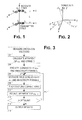
- FIG. 2 demonstrates a rotational transformation definition
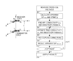
- FIG. 3 shows a flow diagram for the disclosed method of determining formation parameters in a dipping anisotropic earth formation
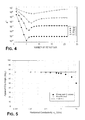
- FIG. 4 shows a graph used to determine the optimal number of iterations that minimize a dip-angle error function
- FIG. 5 compares the results of the disclosed method to results obtained with an existing method.
- FIG. 1 shows a conceptual sketch of a coil arrangement for a downhole induction tool.
- a triad of transmitter coils T x , T y and T z each oriented along a respective axis, is provided, as is a similarly oriented triad of receiver coils R x , R y and R z ,.
- the three coils in each triad represent actual coils oriented in mutually perpendicular directions, with the z-axis corresponding to the long axis of the tool.
- this coil arrangement can be “synthesized” by performing a suitable transformation on differently oriented triads. Such transformations are described in depth in U.S.
- Each of the coils in the transmitter triad is parallel to the corresponding coil in the receiver triad and is spaced away from the corresponding coil in the z-axis direction.
- the distance between the corresponding coils is labeled L.
- the downhole tool may have additional transmitter or receiver triads to provide multiple transmitter-receiver spacing L values. Such configurations may advantageously provide increased accuracy or additional detail useful for analyzing the formation structure.
- a formation model is used to interpret the tool measurements.
- FIG. 2 shows a transformation from the tool coordinate system to the formation coordinate system.
- the tool coordinate system (x,y,z) is first rotated about the z-axis by an angle ⁇ , hereafter termed the strike angle.
- Any vector v′′ in the formation coordinate system can be expressed in the tool coordinate system as:
- H x , H y , H z and M x , M y , M z are the field components at the receivers and magnetic moment components at the transmitters, respectively.
- T x R x ⁇ fraction (M/2+L ) ⁇ [(c xx +c zz )+(c xx ⁇ C zz )cos 2 ⁇ +2C xz sin 2 ⁇ ]cos 2 ⁇ +2C yy sin 2 ⁇ (12)
- T y R y ⁇ fraction (M/2+L ) ⁇ [(C xx +C zz )+(C xx ⁇ C zz )cos 2 ⁇ +2C xz sin 2 ⁇ ]sin 2 ⁇ +2C yy cos 2 ⁇ (13)
- T z R z ⁇ fraction (M/2+L ) ⁇ [(C xx +C zz )+(C zz ⁇ C xx )cos 2 ⁇ 2C xz sin 2 ⁇ ] (14)
- T x R y ⁇ fraction (M/4+L ) ⁇ [(C xx +C zz )+(C xx ⁇ C zz )cos 2 ⁇ +2C xz sin 2 ⁇ 2C yy ]sin 2 ⁇ (15)
- T z R y ⁇ fraction (M/2+L ) ⁇ [(C zz ⁇ C xx )sin 2 ⁇ +2C xz cos 2 ⁇ ]sin ⁇ (17)
- T x R y K V Ry /V Tx , where K is a real-valued calibration constant theoretically equal to A T N T I T A R N R ( ⁇ ) 2 /4 ⁇ L, where A R is the area of the receive coil, and N R is the number of turns of the receive coil.
- Equations (24) and (25) can be solved to obtain A and ⁇ h :
- leading fraction may be replaced by a calibration coefficient K 1 for the tool.
- Equation (24) and (25) are no longer correct.
- the extra skin-effect contribution may be subtracted from the left-hand side.
- ⁇ zx is the higher order correction obtained from (30):
- ⁇ zx M 8 ⁇ ⁇ ⁇ ⁇ L 3 ⁇ cos ⁇ ⁇ ⁇ ⁇ ⁇ sin ⁇ ⁇ 2 ⁇ ⁇ ⁇ a1 sin 2 ⁇ ⁇ a1 ⁇ [ 2 3 ⁇ ( 1 - A a1 3 ) ⁇ ( L ⁇ a1 ) 4 + 1 3 ⁇ ( 1 - A a1 4 ) ⁇ ( L ⁇ a1 ) 5 ] ( 32 )
- a a2 1 1 + ( T z ⁇ R x ) X - ( T z ⁇ R x ) R - ⁇ zx ( T z ⁇ R z ) X - ( T z ⁇ R z ) R - ⁇ zz ⁇ tan ⁇ ⁇ ⁇ a1 cos ⁇ ⁇ ⁇ ( 34 )
- ⁇ h2 4 ⁇ ⁇ ⁇ ⁇ L M ⁇ ⁇ ⁇ ⁇ ⁇ ⁇ [ ( T z ⁇ R x ) X - ( T z ⁇ R x ) R ] A a2 ( 35 )
- Equation (25) The same “extend to a higher order” procedure can be applied to the other components of the measured fields in Equation (25).
- ⁇ h ⁇ Apparent horizontal conductivity
- P ⁇ ( ⁇ a ) ( A a 3 - 1 ) 6 ⁇ ( 1 + cos 2 ⁇ ⁇ a ) sin 2 ⁇ ⁇ a + A a 2 ⁇ ( A a 2 - cos 2 ⁇ ⁇ a ) sin 2 ⁇ ⁇ a - 1 2
- Q ⁇ ( ⁇ a ) ( A a 4 - 1 ) 24 ⁇ ( 1 + cos 2 ⁇ ⁇ a ) sin 2 ⁇ ⁇ a + A a 2 6 ⁇ ( A a 2 - cos 2 ⁇ ⁇ a ) sin 2 ⁇ ⁇ a - 1 6
- Eqn. (36) includes correction terms that are specified by Eqn. (37).
- the property determination approach built into Eqns (34)-(37) is believed to be unknown to the art.
- FIG. 3 shows an iterative method that uses the above equations to determine the dip and strike angles, the horizontal conductivity, and the anisotropy coefficient (calculated from the anisotropic factor).
- the transmitter coils are activated and the voltages produced in the receiver coils are measured. The measured voltages are processed to determine the magnetic couplings between the coils.
- the strike angle ⁇ is calculated per Eqn (20) and the first estimate of the dip angle ⁇ A1 is calculated per Eqn (21).
- the first estimate of the anisotropic factor A A is calculated per Eqn (28) and the first estimate of the horizontal conductivity ⁇ hA is calculated per Eqn (29).
- Blocks 308 through 314 form a loop having a loop index J.
- Loop index J is initialized to 1 for the first iteration of the loop, and incremented by 1 for subsequent iterations of the loop.
- an iterative estimate of the anisotropic factor A J is calculated per Eqn (34) and an iterative estimate of the horizontal conductivity ⁇ hJ is calculated per Eqn (35).
- coupling correction terms are caculated per Eqns (37-a,b,c).
- an iterative estimate of the dip angle ⁇ (J+1) is calculated per Eqn (36) using the coupling correction terms found in block 310 .
- a test is made to determine if the optimum number of iterations has been performed, and if more iterations are needed, control returns to block 308 . Otherwise.
- the anisotropy coefficient ⁇ is calculated from the latest estimates of the dip angle and anisotropic factor (refer to the definition of the anisotropic factor in Eqn (11)). The anisotropy coefficient ⁇ is then output, along with the strike angle ⁇ , and the best estimates of the dip angle ⁇ and horizontal conductivity ⁇ h .
- the effectiveness of the method is demonstrated in Table I where all apparent formation parameters are listed for each successive iteration.
- the sonde is a triad 2C40 (notation means 2 coils spaced 40 inches apart) operating at 8 kHz.
- FIG. 4 shows the apparent dip angle examination results for four triad-pair configurations having different transmitter-receiver spacings.
- the error function is calculated over the following ranges of formation parameters:
- ⁇ h (0.001, 0.01, 0.02, 0.05, 0.1, 0.2, 0.5, 1, 2, 5, 10 S/m)
- ⁇ (1.1, 1.414, 2, 4, 6, 8, 10).
- the optimal iteration number is defined as the iteration number at which the error is minimal. This can similarly be done for the anisotropy coefficient ⁇ and horizontal conductivity ⁇ h to obtain their respective optimal iteration numbers.
- FIG. 5 plots the calculated dip angle measured in dipping formations having different horizontal conductivities.
- the true dip angle of the formation is 75 degrees.
- the original method proposed by Moran and Gianzero has large errors in conductive formations due to the skin effect, while the disclosed method yields a calculated dip angle close to the true dip of 75 degrees.
- the current method also yields the other formation parameters illustrated in Table I.
Landscapes
- Life Sciences & Earth Sciences (AREA)
- Physics & Mathematics (AREA)
- Engineering & Computer Science (AREA)
- Geology (AREA)
- Geophysics (AREA)
- Remote Sensing (AREA)
- Environmental & Geological Engineering (AREA)
- General Life Sciences & Earth Sciences (AREA)
- General Physics & Mathematics (AREA)
- Mining & Mineral Resources (AREA)
- Electromagnetism (AREA)
- Fluid Mechanics (AREA)
- Geochemistry & Mineralogy (AREA)
- Investigating Or Analyzing Materials By The Use Of Electric Means (AREA)
- Geophysics And Detection Of Objects (AREA)
- Measurement Of Resistance Or Impedance (AREA)
- Investigating Or Analyzing Materials By The Use Of Magnetic Means (AREA)
Abstract
A method is disclosed for the determination of horizontal resistivity, vertical resistivity, dip and strike angles of anisotropic earth formations surrounding a wellbore. Electromagnetic couplings among a plural of triad transmitters and triad receivers are measured. Each triad transmitter/receiver consists of coil windings in three mutually orthogonal axes. These measured signals are used to generate initial estimates of the dip angle and strike angle of the formation as well as the anisotropy coefficient and the horizontal resistivity of the formation. An iterative algorithm is then applied using these quantities to finally arrive at more accurate estimates that approach the true values in the formation.
Description
1. Field of the Invention
The present invention generally relates to the measurement of electrical characteristics of formations surrounding a wellbore. More particularly, the present invention relates to a method for determining horizontal and vertical resistivities in anisotropic formations while accounting for the dip and stike angle of the formation.
2. Description of the Related Art
The basic principles and techniques for electromagnetic logging for earth formations are well known. Induction logging to determine the resistivity (or its inverse, conductivity) of earth formations adjacent a borehole, for example, has long been a standard and important technique in the search for and recovery of subterranean petroleum deposits. In brief, the measurements are made by inducing eddy currents to flow in the formations in response to an AC transmitter signal, and then measuring the appropriate characteristics of a receiver signal generated by the formation eddy currents. The formation properties identified by these signals are then recorded in a log at the surface as a function of the depth of the tool in the borehole.
It is well known that subterranean formations surrounding an earth borehole may be anisotropic with regard to the conduction of electrical currents. The phenomenon of electrical anisotropy is generally a consequence of either microscopic or macroscopic geometry, or a combination thereof, as follows.
In many sedimentary strata, electrical current flows more easily in a direction parallel to the bedding planes, as opposed to a direction perpendicular to the bedding planes. One reason is that a great number of mineral crystals possess a flat or elongated shape (e.g., mica or kaolin). At the time they were laid down, they naturally took on an orientation parallel to the plane of sedimentation. The interstices in the formations are, therefore, generally parallel to the bedding plane, and the current is able to easily travel along these interstices which often contain electrically conductive mineralized water. Such electrical anisotropy, sometimes called microscopic anisotropy, is observed mostly in shales.
Subterranean formation are often made up of a series of relatively thin beds having different lithological characteristics and, therefore different resistivities. In well logging systems, the distances between the electrodes or antennas are great enough that the volume involved in a measurement may include several such thin beds. When individual layers are neither delineated nor resolved by a logging tool, the tool responds to the formation as if it were a macroscopically anisotropic formation. A thinly laminated sand/shale sequence is a particularly important example of a macroscopically anisotropic formation.
If a sample is cut from a subterranean formation, the resistivity of the sample measured with current flowing parallel to the bedding planes is called the transverse or horizontal resistivity ρH. The inverse of ρH is the horizontal conductivity σH. The resistivity of the sample measured with a current flowing perpendicular to the bedding plane is called the longitudinal or vertical resistivity, ρV, and its inverse the vertical conductivity σV. The anisotropy coefficient λ is defined as: λ={square root over (σh+L /σv+L )}.
In situations where the borehole intersects the formation substantially perpendicular to the bedding planes, conventional induction and propagation well logging tools are sensitive almost exclusively to the horizontal component of the formation resistivity. When the borehole intersects the bedding planes at an angle (a deviated borehole) the tool readings contain an influence from the vertical and horizontal resistivities. This is particularly true when the angle between the borehole and the normal to the bedding places is large, such as in directional or horizontal drilling, where angles near 90° are commonly encountered. In these situations, the influence of vertical resistivity can cause discrepancies between measurements taken in the same formation in nearby vertical wells, thereby preventing a useful comparison of these measurements. In addition, since reservoir evaluation is typically based on data obtained from vertical wells, the use of data from wells drilled at high angles may produce erroneous estimates of formation reserve, producibility, etc. if proper account is not taken of the anisotropy effect.
There have been proposed a number of methods to determine vertical and horizontal resistivity near a deviated borehole. Hagiwara (U.S. Pat. No. 5,966,013) disclosed a method of determining certain anisotropic properties of formation using propagation tool without a priori knowledge of the dip angle. In U.S. Pat. No. 5,886,526, Wu described a method of determining anisotropic properties of anisotropic earth formations using multi-spacing induction tool with assumed functional dependence between dielectric constants of the formation and its horizontal and vertical resistivity. Gupta et al. (U.S. Pat. No. 5,999,883) utilized a triad induction tool to arrive at an approximate initial guesses for the anisotropic formation parameters. Moran and Gianzero (Geophysics, Vol. 44, P. 1266, 1979) proposed using a tri-axial tool of zero spacing to determine dip angle. Later the spacing was extended to finite size by Gianzero et al. (U.S. Pat. No. 5,115,198) using a pulsed induction tool. The above references are hereby incorporated herein by reference.
These attempts to determine vertical and horizontal resistivity around a deviated borehole have thus far not provided sufficient accuracy for formations having a high degree of anisotropy. A new technique is therefore needed.
The above-described problems are in large part addressed by an iterative method for determining electrical conductivity in an anisotropic dipping formation. The iterative method corrects for the skin effect to high orders while determining all relevant formation parameters. This method may be applied to a tri-axial induction sonde operating in continuous wave (CW) mode. In one embodiment, the method includes (1) measuring a magnetic coupling between transmitter coils and receiver coils of a tool in a borehole traversing the formation; (2) obtaining from the measured coupling a strike angle between the tool and the formation; (3) obtaining from the measured coupling an initial dip angle between the tool and the formation; (4) obtaining from the measured coupling an initial anisotropic factor of the formation; (5) obtaining from the measured coupling an initial horizontal conductivity of the formation; (6) determining an iterative anisotropic factor from the measured coupling, the strike angle, the latest dip angle, and the latest anistropic factor; (7) determining an iterative horizontal conductivity from the measured coupling, the strike angle, the latest iterative anisotropic factor, and the latest dip angle; and (8) determining an iterative dip angle from the measured coupling, the latest iterative anisotropic factor, and the latest iterative horizontal conductivity. The steps of determining an iterative anisotropic factor, determining an iterative horizontal conductivity, and determining an iterative dip angle are preferably repeated a number of times that minimizes an overall residual error.
The disclosed method may provide the following advantages in determining the formation parameters of anisotropic earth formations: (1) a priori knowledge of the dip angle is unnecessary and can be one of the outputs of the method; (2) no assumed relationship between formation resistivity and dielectric constant is necessary; (3) complex electronics for pulsing the transmitter coils may be eliminated since this method is applicable to a triad induction sonde running in CW mode; (4) preliminary results indicate that the disclosed method yields more accurate estimates of all electrically relevant formation parameters in the earth formation.
A better understanding of the present invention can be obtained when the following detailed description of the preferred embodiment is considered in conjunction with the following drawings, in which:
FIG. 1 shows the coil configuration of a triazial induction tool;
FIG. 2 demonstrates a rotational transformation definition;
FIG. 3 shows a flow diagram for the disclosed method of determining formation parameters in a dipping anisotropic earth formation;
FIG. 4 shows a graph used to determine the optimal number of iterations that minimize a dip-angle error function; and
FIG. 5 compares the results of the disclosed method to results obtained with an existing method.
While the invention is susceptible to various modifications and alternative forms, specific embodiments thereof are shown by way of example in the drawings and will herein be described in detail. It should be understood, however, that the drawings and detailed description thereto are not intended to limit the invention to the particular form disclosed, but on the contrary, the intention is to cover all modifications, equivalents and alternatives falling within the spirit and scope of the present invention as defined by the appended claims.
It is noted that the terms horizontal and vertical as used herein are defined to be those directions parallel to and perpendicular to the bedding plane, respectively.
Turning now to the figures, FIG. 1 shows a conceptual sketch of a coil arrangement for a downhole induction tool. A triad of transmitter coils Tx, Ty and Tz, each oriented along a respective axis, is provided, as is a similarly oriented triad of receiver coils Rx, Ry and Rz,. For clarity, it is assumed that the three coils in each triad represent actual coils oriented in mutually perpendicular directions, with the z-axis corresponding to the long axis of the tool. However, it is noted that this coil arrangement can be “synthesized” by performing a suitable transformation on differently oriented triads. Such transformations are described in depth in U.S. patent application Ser. No. 09/255,621 entitled “Directional Resistivity Measurements for Azimutal Proximity Detection of Bed Boundaries” and filed Feb. 22, 1999 by T. Hagiwara and H. Song, which is hereby incorporated herein by reference.
Each of the coils in the transmitter triad is parallel to the corresponding coil in the receiver triad and is spaced away from the corresponding coil in the z-axis direction. The distance between the corresponding coils is labeled L. It is noted that the downhole tool may have additional transmitter or receiver triads to provide multiple transmitter-receiver spacing L values. Such configurations may advantageously provide increased accuracy or additional detail useful for analyzing the formation structure.
Generally, a formation model is used to interpret the tool measurements. The model used herein is a unixial anisotropy model. This model assumes that the formation is isotropic in the horizontal direction (parallel to the bedding plane) and anisotropic in the vertical direction (perpendicular to the bedding plane). Setting up a formation coordinate system having the z-axis perpendicular to the bedding plane and the x- and y-axes parallel to the bedding plane allows a conductivity tensor to be expressed as: 
The axes of the formation coordinate system typically do not correspond to the axes of the tool coordinate system. However, a rotational transformation from one to the other can be defined. FIG. 2 shows a transformation from the tool coordinate system to the formation coordinate system. The tool coordinate system (x,y,z) is first rotated about the z-axis by an angle β, hereafter termed the strike angle. The intermediate coordinate system (x′,y′,z′=z) thus formed is then rotated about the y′ axis by an angle α, hereafter termed the dip angle to obtain the formation coordinate system (x″,y″=y′,z″).
Any vector v″ in the formation coordinate system can be expressed in the tool coordinate system as:
where the rotational transform matrix is: 
Now that the rotational transformation has been defined, attention is directed to the induction tool measurements. When a voltage is applied to one of the transmitter coils, a changing magnetic field is produced. The magnetic field interacts with the formation to induce a voltage in the receiver coils. Each of the three transmitter coils is excited in turn, and the voltage produced at each of the three receiver coils is measured. The nine measured voltages indicate the magnetic coupling between the transmitter-receiver triad pair. The equations for the measured signals will be derived and manipulated to solve for the strike angle β, the dip angle α, the horizontal conductivity σh, and the vertical anisotropy λ.
In the most general case according to Moran and Gianzero (Geophysics, Vol. 44, P. 1266, 1979), the magnetic field H in the receiver coils can be represented as a coupling matrix C in the form: 
where Hx, Hy, Hz and Mx, My, Mz, are the field components at the receivers and magnetic moment components at the transmitters, respectively. (Magnetic moment is calculated MT=ATNTIT, where AT is the transmitter area, NT is the number of turns in the transmitter coil, and IT is the transmitter current. The direction of the magnetic moment is perpendicular to the plane of the coil). If the coupling matrix is specified in terms of the formation coordinate system, the measured magnetic field strengths in the receiver coils are obtained by (Moran and Gianzero, Geophysics, Vol. 44, P. 1266, 1979):
where H and M are measured in the sonde coordinate system.
Assuming that the tool is oriented so that the strike angle β is 0, it can be shown that for the uniaxial anisotropy model the full coupling matrix C′ at the receiver coils (x=0=y, z=L) simplifies to 
The theoretical values of the coupling matrix elements are (Cij=Cji): 
where
kh={square root over (ωμσh+L )}=horizontal wave number
ω=2πƒ=angular frequency
μ=μ0=4π×10−7 henry/m=magnetic permeability
λ={square root over (σh+L /σv+L )}=anisotropy coefficient
A={square root over (sin2 +L α+λ2 +L cos2 +L α)}/λ=anisotropic factor
In terms of the elements of the coupling matrix C′, the six independent measurements for all the possible couplings between all transmitter-receiver pairs are expressed as (TiRj=TjRi):
These measurements are made by taking the ratio of the transmit and receive voltage signals, e.g. TxRy=K VRy/VTx, where K is a real-valued calibration constant theoretically equal to ATNTITARNR(ωμ)2/4πL, where AR is the area of the receive coil, and NR is the number of turns of the receive coil.
Explicitly solving the last four of the above equations results in the following expressions for the measured cross-coupling fields: 
To make practical use of the above equations, the real component is ignored and the imaginary (reactive) component is simplified by finding the limit as the transmitter-receiver spacing approaches zero, i.e., L→0. Doing this simplifies the reactive components of the measured signal equations (18-a,b,c) to: 
where δh ={square root over (2+L /ωμσh+L )} is the skin depth associated with horizontal conductivity. From these equations, one arrives at the practical equations for the determination of dip and strike angles: 
It is noted that the strike angle β thus obtained is exact while the dip angle α is only an approximation because Equations (19a-c) are valid only in the zero-spacing limit. The subscript α1 denotes that this is the first approximation of the apparent dip angle.
With the strike angle β and the estimated dip angle α, estimates of the horizontal conductivity σh and anisotropy factor A can be obtained via the following observation.
When a power series expansion is used for the exponential terms in equation (18-b), the first terms yield the following expressions for the real part (TzRx)R and imaginary part (TzRx)X. 
Taking advantage of the fact that the second term in (TzRx)X is identical to (TzRx)R, an equation that is skin-effect corrected to the first order can be written as: 
Similarly with equation (18-d), for TzRz one has: 
Equations (24) and (25) can be solved to obtain A and σh: 
Substituting the strike angle β and the first estimate of the dip angle αα1 from Equations (20) and (21) yields the first estimates of the anisotropic factor Aα1 and the horizontal conductivity σh1, where the subscript α1 denotes the quantities are the first estimates of the apparent values: 
It is noted that the leading fraction may be replaced by a calibration coefficient K1 for the tool.
Now that initial estimates have been obtained, the estimates can be iteratively improved. Examining the series expansion of all the measured fields reveals that 
Because the higher order terms do not cancel each other, Equations (24) and (25) are no longer correct. To remedy this problem, the extra skin-effect contribution may be subtracted from the left-hand side. Namely, the left-hand side of Equation (24) may be replaced by (TzRx)R−(TzRx)X−Γzx where Γzx is the higher order correction obtained from (30): 
Similarly, the correction for (TzRz)R−(TzRz)X can be derived: 
It is noted that the leading fraction in (32) and (33) may be replaced with a calibration coefficient K2 and 2K2, respectively, for the tool. With these corrections, one gets better approximations for A and σh: 
The same “extend to a higher order” procedure can be applied to the other components of the measured fields in Equation (25). The end result is a more accurate equation for the dip angle: 
It is noted that here the real part of the magnetic field (which is identical to the imaginary part of the measured voltages at the coils other than a constant factor) is used, hence the subscript R. The correction terms can be directly obtained from the 6th order expansions of the corresponding coupling fields. The correction terms are: 
where
αα=Apparent dip angle 
σhα=Apparent horizontal conductivity 
Property Determination Method
The above derivation has provided:
Eqn. (20) for the determination of the strike angle β,
Eqn. (21) for a first estimate of the dip angle α,
Eqn. (28) for a first estimate of the anisotropic factor A,
Eqn. (29) for a first estimate of the horizontal conductivity σ,
Eqn. (34) for an iterative estimate of the anisotropic factor A,
Eqn. (35) for an iterative estimate of the horizontal conductivity σ, and
Eqn. (36) for an iterative estimate of the dip angle α.
Eqn. (36) includes correction terms that are specified by Eqn. (37). The property determination approach built into Eqns (34)-(37) is believed to be unknown to the art.
FIG. 3 shows an iterative method that uses the above equations to determine the dip and strike angles, the horizontal conductivity, and the anisotropy coefficient (calculated from the anisotropic factor). In block 302, the transmitter coils are activated and the voltages produced in the receiver coils are measured. The measured voltages are processed to determine the magnetic couplings between the coils. In block 304, the strike angle β is calculated per Eqn (20) and the first estimate of the dip angle αA1 is calculated per Eqn (21). In block 306, the first estimate of the anisotropic factor AA is calculated per Eqn (28) and the first estimate of the horizontal conductivity σhA is calculated per Eqn (29).
In block 308, an iterative estimate of the anisotropic factor AJ is calculated per Eqn (34) and an iterative estimate of the horizontal conductivity σhJ is calculated per Eqn (35). In block 310, coupling correction terms are caculated per Eqns (37-a,b,c). In block 312, an iterative estimate of the dip angle α(J+1) is calculated per Eqn (36) using the coupling correction terms found in block 310. In block 314, a test is made to determine if the optimum number of iterations has been performed, and if more iterations are needed, control returns to block 308. Otherwise. in block 316, the anisotropy coefficient λ is calculated from the latest estimates of the dip angle and anisotropic factor (refer to the definition of the anisotropic factor in Eqn (11)). The anisotropy coefficient λ is then output, along with the strike angle β, and the best estimates of the dip angle α and horizontal conductivity σh.
Analysis of Method
The effectiveness of the method is demonstrated in Table I where all apparent formation parameters are listed for each successive iteration. The true formation parameters are: dip angle α=45°, strike angle β=60°, anisotropy coefficient λ=2, and horizontal conductivity σh=5 S/m. The sonde is a triad 2C40 (notation means 2 coils spaced 40 inches apart) operating at 8 kHz.
| TABLE I |
| Effect of iteration number for triad 2C40 in a dipping |
| anisotropic formation. |
| Iteration No. | Apparent Dip αα | Apparent λ | |
| 0 | 34.72° | 4.71 | 9.234 |
| 1 | 39.21° | 1.916 | 4.752 |
| 2 | 41.74° | 1.968 | 4.890 |
| 3 | 43.22° | 1.992 | 4.975 |
| 4 | 44.11° | 2.005 | 5.029 |
| 5 | 44.65° | 2.013 | 5.060 |
| 6 | 44.99° | 2.017 | 5.083 |
| 7 | 45.19° | 2.020 | 5.095 |
| 8 | 45.32° | 2.021 | 5.104 |
| 9 | 45.40° | 2.022 | 5.109 |
| True Values | 45.00° | 2.000 | 5.000 |
A close examination of Table I reveals that there exists an optimal iteration number for each formation parameter beyond which the accuracy of apparent formation parameter actually decreases. For a given triad sonde, the optimal number of iterations for a given parameter can be calculated with the following method. For the three formation parameters, their corresponding error functions are defined as: 
The summations are performed over the range of expected formation dip angles, conductivities, and anisotropy coefficients. This error function is consequently indicative of the overall residual error.
Given a configuration of a triad sonde, the functional dependence of the error function on the number of iterations can be examined. FIG. 4 shows the apparent dip angle examination results for four triad-pair configurations having different transmitter-receiver spacings. The error function is calculated over the following ranges of formation parameters:
α=(5, 15, 30, 45, 60, 75, 85°)
σh=(0.001, 0.01, 0.02, 0.05, 0.1, 0.2, 0.5, 1, 2, 5, 10 S/m)
λ=(1.1, 1.414, 2, 4, 6, 8, 10).
The optimal iteration number is defined as the iteration number at which the error is minimal. This can similarly be done for the anisotropy coefficient λ and horizontal conductivity σh to obtain their respective optimal iteration numbers.
With the optimal iteration number determined, the advantage of the current invention in the dip angle determination over an existing method (Moran and Gianzero, Geophysics, Vol. 44, P. 1266, 1979) can be demonstrated. FIG. 5 plots the calculated dip angle measured in dipping formations having different horizontal conductivities. The true dip angle of the formation is 75 degrees. It is noted that the original method proposed by Moran and Gianzero has large errors in conductive formations due to the skin effect, while the disclosed method yields a calculated dip angle close to the true dip of 75 degrees. It is further emphasized that in addition to a more accurate dip angle, the current method also yields the other formation parameters illustrated in Table I.
Numerous variations and modifications will become apparent to those skilled in the art once the above disclosure is fully appreciated. It is intended that the following claims be interpreted to embrace all such variations and modifications.
Claims (19)
1. A method for determining conductivity in a formation, wherein the method comprises:
measuring a magnetic coupling between transmitter coils and receiver coils of a tool in a borehole traversing the formation;
obtaining from the measured coupling a strike angle between the tool and the formation;
obtaining from the measured coupling an initial dip angle between the tool and the formation;
obtaining from the measured coupling an initial anisotropic factor of the formation;
obtaining from the measured coupling an initial horizontal conductivity of the formation;
determining an iterative anisotropic factor from the measured coupling, the strike angle, the latest dip angle, and the latest anistropic factor;
determining an iterative horizontal conductivity from the measured coupling, the strike angle, the latest iterative anisotropic factor, and the latest dip angle; and
determining an iterative dip angle from the measured coupling, the latest iterative anisotropic factor, and the latest iterative horizontal conductivity.
2. The method of claim 1 , further comprising:
repeating the steps of determining an iterative anisotropic factor, determining an iterative horizontal conductivity, and determining an iterative dip angle.
3. The method of claim 2 , wherein said repeating is performed a number of times that minimizes an overall residual error.
4. The method of claim 1 , wherein the strike angle β corresponds to 
wherein (TzRy)X is the reactive component of the coupling TzRy between a transmitter Tz oriented along a z-axis and a receiver Ry oriented along a y-axis, and (TzRx)X is the reactive component of the coupling TzRx between transmitter Tz and a receiver Rx oriented along an x-axis.
5. The method of claim 1 , wherein the initial dip angle α1 corresponds to 
wherein (TxRy)X is the reactive component of the coupling TxRy between a transmitter Tx oriented along an x-axis and a receiver Ry oriented along a y-axis, (TzRx)X is the reactive component of the coupling TzRx between a transmitter Tz oriented along a z-axis and a receiver Rx oriented along the x-axis, and (TzRy)X is the reactive component of the coupling TzRy between transmitter Tz and receiver Ry.
6. The method of claim 1 , wherein the initial anisotropic factor A1 corresponds to 
wherein (TzRx)X and (TzRx)R are the imaginary and real components, respectively, of the coupling TzRx between a transmitter Tz oriented along a z-axis and a receiver Rx oriented along an x-axis, (TzRz)X and (TzRz)R are the imaginary and real components, respectively, of the coupling TzRz between transmitter Tz and a receiver Rz oriented along the z-axis, α1 is the initial dip angle, and β is the strike angle.
7. The method of claim 1 , wherein the initial horizontal conductivity σh1 corresponds to 
wherein (TzRx)X and (TzRx)R are the imaginary and real components, respectively, of the coupling TzRx between a transmitter Tz oriented along a z-axis and a receiver Rx oriented along an x-axis, A1 is the initial anisotropic factor, and K1 is a predetermined function of transmitter signal voltage and frequency.
8. The method of claim 1 , wherein the iterative anisotropic factor Ai+1 corresponds to 
wherein (TzRx)X and (TzRx)R are the imaginary and real components, respectively, of the coupling TzRx between a transmitter Tz oriented along a z-axis and a receiver Rx oriented along an x-axis, (TzRz)X and (TzRz)R are the imaginary and real components, respectively, of the coupling TzRz between transmitter Tz and a receiver Rz oriented along the z-axis, αi is the latest dip angle, β is the strike angle, Γzx is a first skin-effect correction, and Γzz is a second skin effect correction.
9. The method of claim 8 , wherein the first skin-effect correction Γzx corresponds to 
and the second skin-effect correction corresponds to 
wherein L is a distance between the transmitter and receiver, Ai is the latest anistropic factor, δhi ={square root over (2+L /ωμσhi+L )} is the latest skin depth, σ hi is the latest horizontal conductivity, and K2 is a predetermined function of transmitter signal voltage.
10. The method of claim 1 , wherein the iterative horizontal conductivity σh(i−1) corresponds to 
wherein (TzRx)X and (TzRx)R are the imaginary and real components, respectively, of the coupling TzRx between a transmitter Tz oriented along a z-axis and a receiver Rx oriented along an x-axis, Ai−1 is the latest anisotropic factor, L is a distance between the transmitter and receiver, and K1 is a predetermined function of transmitter signal voltage and frequency.
11. The method of claim 1 , wherein the iterative dip angle αi+1 corresponds to 
wherein (TxRy)R is the real component of the coupling TxRy between a transmitter Tx oriented along an x-axis and a receiver Ry oriented along a y-axis, (TzRx)R is the real component of the coupling TzRx between a transmitter Tz oriented along a z-axis and a receiver Rx oriented along the x-axis, (TzRy)R is the real component of the coupling TzRy between transmitter Tz and receiver Ry, (Δxy)R is a first correction term, (Δzx)R is a second correction term, and (Δzy)R is a third correction term.
12. The method of claim 11 , wherein the first correction term (Δxy)R corresponds to 
wherein the second correction term (Δzx)R corresponds to 
and wherein the third correction term (Δzy)R corresponds to 
wherein αi is the latest dip angle, β is the strike angle, L is a distance between the transmitter and receiver, Ai−1 is the latest anistropic factor, δh(i+1)={square root over (2+L /ωμσh(i+1)+L )} is the latest skin depth, σ h(i+1) is the latest horizontal conductivity, and K2 is a predetermined function of transmitter signal voltage.
13. The method of claim 1 , wherein the transmitter coils consist of a triad of mutually orthogonal transmitters.
14. The method of claim 13 , wherein the receiver coils consist of a triad of mutually orthogonal receivers.
15. The method of claim 1 , wherein said measuring includes exciting each transmitter coil in turn and measuring in-phase and quadrature phase voltage signals induced in each of the receiver coils by each of the transmitter coils.
16. A method for determining conductivity in a formation, wherein the method comprises:
receiving magnetic coupling measurements from an induction tool;
obtaining from the magnetic coupling measurements an initial horizontal conductivity of the formation;
determining an iterative horizontal conductivity from the magnetic coupling measurements and the initial horizontal conductivity of the formation, wherein the initial horizontal conductivity σh1 corresponds to 
wherein K1 is a predetermined function of transmitter signal voltage and frequency, (TzRx)X and (TzRx)R are the imaginary and real components, respectively, of the magnetic coupling measurement TzRx between a transmitter Tz oriented along a z-axis and a receiver Rx oriented along an x-axis, and A1 is the initial anisotropic factor corresponding to 
wherein the strike angle β corresponds to 
and the initial dip angle α1 corresponds to 
wherein (TzRz)X and (TzRz)R are the imaginary and real components, respectively, of the coupling TzRz between transmitter Tz and a receiver Rz oriented along the z-axis, wherein (TxRy)X is the reactive component of the coupling TxRy between a transmitter Tx oriented along the x-axis and a receiver Ry oriented along a y-axis, wherein (TzRy)X is the reactive component of the coupling TzRy between transmitter Tz and receiver Ry.
17. A method for determining conductivity in a formation, wherein the method comprises:
receiving magnetic coupling measurements from an induction tool;
obtaining from the magnetic coupling measurements an initial horizontal conductivity of the formation;
determining an iterative horizontal conductivity from the magnetic coupling measurements and the initial horizontal conductivity of the formation, wherein the iterative horizontal conductivity σh(i+1) corresponds to 
wherein K1 is a predetermined function of transmitter signal voltage and frequency, wherein (TzRx)X and (TzRx)R are the imaginary and real components, respectively, of the coupling TzRx between a transmitter Tz oriented along a z-axis and a receiver Rx oriented along an x-axis, and Ai+1 corresponds to 
wherein (TzRz)X and (TzRz)R are the imaginary and real components, respectively, of the coupling TzRz between transmitter Tz and a receiver Rz oriented along the z-axis, Γzx is a first skin-effect correction, Γzz is a second skin effect correction, the strike angle β corresponds to 
and the dip angle αi corresponds to 
wherein (TzRy)X and (TzRy)R are the imaginary and real components, respectively, of the coupling TzRy between transmitter Tz and a receiver Ry oriented along a y-axis, (TxRy)R is the real component of the coupling TxRy between a transmitter Tx oriented along the x-axis and receiver Ry, (Δxy)R is a first correction term, (Δzx)R is a second correction term, and (Δzy)R is a third correction term.
18. The method of claim 17 , wherein the first skin-effect correction Γzx corresponds to 
and the second skin-effect correction corresponds to 
wherein L is a distance between the transmitter and receiver, Ai is the latest anistropic factor, δhi ={square root over (2/ωμσhi+L )} is the latest skin depth, σ hi is the latest horizontal conductivity, and K2 is a predetermined function of transmitter signal voltage.
19. The method of claim 17 , wherein the first correction term (Δxy)R corresponds to 
wherein the second correction term (Δzx)R corresponds to 
and wherein the third correction term (Δzy)R corresponds to 
wherein αi is the latest dip angle, β is the strike angle, L is a distance between the transmitter and receiver, Ai is the latest anistropic factor, δhi ={square root over (2+L /ωμσhi+L )} is the latest skin depth, σ hi is the latest horizontal conductivity, K2 is a predetermined function of transmitter signal voltage.
Priority Applications (7)
| Application Number | Priority Date | Filing Date | Title |
|---|---|---|---|
| US09/583,184 US6393364B1 (en) | 2000-05-30 | 2000-05-30 | Determination of conductivity in anisotropic dipping formations from magnetic coupling measurements |
| AU43911/01A AU775118B2 (en) | 2000-05-30 | 2001-05-16 | Method for iterative determination of conductivity in anisotropic dipping formations |
| CA002348204A CA2348204C (en) | 2000-05-30 | 2001-05-18 | Method for iterative determination of conductivity in anisotropic dipping formations |
| GB0112451A GB2367366B (en) | 2000-05-30 | 2001-05-22 | Method for iterative determination of conductivity in anisotropic dipping formations |
| NO20012627A NO20012627L (en) | 2000-05-30 | 2001-05-29 | Method for iterative determination of conductivity in anisotropic falling formations |
| FR0106999A FR2809825B1 (en) | 2000-05-30 | 2001-05-29 | METHOD FOR THE ITERATIVE DETERMINATION OF CONDUCTIVITY IN INCLINED ANISOTROPIC FORMATIONS |
| BR0102181-8A BR0102181A (en) | 2000-05-30 | 2001-05-30 | Process of determining conductivity in a formation |
Applications Claiming Priority (1)
| Application Number | Priority Date | Filing Date | Title |
|---|---|---|---|
| US09/583,184 US6393364B1 (en) | 2000-05-30 | 2000-05-30 | Determination of conductivity in anisotropic dipping formations from magnetic coupling measurements |
Publications (1)
| Publication Number | Publication Date |
|---|---|
| US6393364B1 true US6393364B1 (en) | 2002-05-21 |
Family
ID=24332022
Family Applications (1)
| Application Number | Title | Priority Date | Filing Date |
|---|---|---|---|
| US09/583,184 Expired - Lifetime US6393364B1 (en) | 2000-05-30 | 2000-05-30 | Determination of conductivity in anisotropic dipping formations from magnetic coupling measurements |
Country Status (7)
| Country | Link |
|---|---|
| US (1) | US6393364B1 (en) |
| AU (1) | AU775118B2 (en) |
| BR (1) | BR0102181A (en) |
| CA (1) | CA2348204C (en) |
| FR (1) | FR2809825B1 (en) |
| GB (1) | GB2367366B (en) |
| NO (1) | NO20012627L (en) |
Cited By (43)
| Publication number | Priority date | Publication date | Assignee | Title |
|---|---|---|---|---|
| WO2002082353A1 (en) * | 2001-04-03 | 2002-10-17 | Baker Hughes Incorporated | Determination of formation anisotropy using multi-frequency processing of induction measurements with transverse induction coils |
| US6556015B1 (en) * | 2001-10-11 | 2003-04-29 | Schlumberger Technology Corporation | Method and system for determining formation anisotropic resistivity with reduced borehole effects from tilted or transverse magnetic dipoles |
| US6556016B2 (en) * | 2001-08-10 | 2003-04-29 | Halliburton Energy Services, Inc. | Induction method for determining dip angle in subterranean earth formations |
| US20030105591A1 (en) * | 2001-12-03 | 2003-06-05 | Teruhiko Hagiwara | Method for determining anisotropic resistivity and dip angle in an earth formation |
| US6584408B2 (en) * | 2001-06-26 | 2003-06-24 | Schlumberger Technology Corporation | Subsurface formation parameters from tri-axial measurements |
| US20030200029A1 (en) * | 2002-04-19 | 2003-10-23 | Dzevat Omeragic | Subsurface formation anisotropy determination with tilted or transverse magnetic dipole antennas |
| WO2003100466A1 (en) * | 2002-05-20 | 2003-12-04 | Halliburton Energy Services, Inc. | Induction well logging apparatus and method |
| WO2004003593A1 (en) * | 2002-07-01 | 2004-01-08 | Baker Hugues Incorporated | Method for joint interpretation of multi-array induction and multi-component induction measurements with joint dip angle estimation |
| US20040017197A1 (en) * | 2002-07-29 | 2004-01-29 | Schlumberger Technology Corporation | Co-located antennas |
| US20040059515A1 (en) * | 2002-07-10 | 2004-03-25 | Exxonmobil Upstream Research Company | Apparatus and method for measurment of the magnetic induction tensor using triaxial induction arrays |
| US6727706B2 (en) * | 2001-08-09 | 2004-04-27 | Halliburton Energy Services, Inc. | Virtual steering of induction tool for determination of formation dip angle |
| US20040113609A1 (en) * | 2002-07-30 | 2004-06-17 | Homan Dean M. | Electromagnetic logging tool calibration system |
| US20040138819A1 (en) * | 2003-01-09 | 2004-07-15 | Goswami Jaideva C. | Method and apparatus for determining regional dip properties |
| US20040155660A1 (en) * | 2002-12-31 | 2004-08-12 | Schlumberger Technology Corporation | System and method for locating a fracture in an earth formation |
| US6795774B2 (en) | 2002-10-30 | 2004-09-21 | Halliburton Energy Services, Inc. | Method for asymptotic dipping correction |
| US20050049792A1 (en) * | 2003-08-29 | 2005-03-03 | Baker Hughes Incorporated | Real time processing of multicomponent induction tool data in highly deviated and horizontal wells |
| US20050114030A1 (en) * | 2002-08-19 | 2005-05-26 | Schlumberger Technology Corporation | [methods and systems for resistivity anisotropy formation analysis] |
| US20050274512A1 (en) * | 2004-06-15 | 2005-12-15 | Baker Hughes Incorporated | Determination of formation anistropy, dip and azimuth |
| US20060082374A1 (en) * | 2004-10-15 | 2006-04-20 | Jiaqi Xiao | Minimizing the effect of borehole current in tensor induction logging tools |
| US20060253255A1 (en) * | 2005-04-22 | 2006-11-09 | Schlumberger Technology Corporation | Anti-symmetrized electromagnetic measurements |
| US20070208546A1 (en) * | 2006-03-06 | 2007-09-06 | Sheng Fang | Real time data quality control and determination of formation angles from multicomponent induction measurements using neural networks |
| US20070219723A1 (en) * | 2004-06-15 | 2007-09-20 | Baker Hughes Incorporated | Geosteering In Earth Formations Using Multicomponent Induction Measurements |
| US7286091B2 (en) | 2003-06-13 | 2007-10-23 | Schlumberger Technology Corporation | Co-located antennas |
| US20080129093A1 (en) * | 2006-12-05 | 2008-06-05 | Seok Hwan Kim | Device maintaining height of an active headrest |
| US20080215243A1 (en) * | 2004-06-15 | 2008-09-04 | Baker Hughes Incorporated | Processing of Multi-Component Induction Measurements in a Biaxially Anisotropic Formation |
| US20080211507A1 (en) * | 2004-02-23 | 2008-09-04 | Michael Zhdanov | Method and Apparatus for Gradient Electromagnetic Induction Well Logging |
| US20080314582A1 (en) * | 2007-06-21 | 2008-12-25 | Schlumberger Technology Corporation | Targeted measurements for formation evaluation and reservoir characterization |
| US20090018775A1 (en) * | 2004-06-15 | 2009-01-15 | Baker Hughes Incorporated | Geosteering in Earth Formations Using Multicomponent Induction Measurements |
| US20090192713A1 (en) * | 2008-01-25 | 2009-07-30 | Baker Hughes Incorporated | Determining Structural Dip and Azimuth From LWD Resistivity Measurements in Anisotropic Formations |
| US7765067B2 (en) | 2004-06-15 | 2010-07-27 | Baker Hughes Incorporated | Geosteering in earth formations using multicomponent induction measurements |
| WO2012150934A1 (en) | 2011-05-03 | 2012-11-08 | Halliburton Energy Services, Inc. | Method for estimating formation parameters from imaginary components of measured data |
| WO2013015789A1 (en) * | 2011-07-26 | 2013-01-31 | Halliburton Energy Services, Inc. | Cross-coupling based determination of anisotropic formation properties |
| CN102979519A (en) * | 2012-12-14 | 2013-03-20 | 中国电子科技集团公司第二十二研究所 | Method and device for measuring resistivity of resistivity equipment with tilt coil |
| US20140025357A1 (en) * | 2011-02-02 | 2014-01-23 | Statoil Petroleum As | Method of predicting the response of an induction logging tool |
| WO2014098838A1 (en) * | 2012-12-19 | 2014-06-26 | Halliburton Energy Services, Inc. | Method and apparatus for optimizing deep resistivity measurements with multi-component antennas |
| WO2014113008A1 (en) * | 2013-01-17 | 2014-07-24 | Halliburton Energy Services, Inc. | Fast formation dip angle estimation systems and methods |
| US20150047902A1 (en) * | 2011-09-27 | 2015-02-19 | Halliburton Energy Services, Inc. | Systems and methods of robust determination of boundaries |
| US20150134256A1 (en) * | 2013-11-11 | 2015-05-14 | Baker Hughes Incorporated | Late time rotation processing of multi-component transient em data for formation dip and azimuth |
| EP2751600A4 (en) * | 2011-10-31 | 2015-07-29 | Halliburton Energy Services Inc | Multi-component induction logging systems and methods using real-time obm borehole correction |
| CN109342978A (en) * | 2018-11-06 | 2019-02-15 | 中国石油天然气集团有限公司 | Magnetotelluric anisotropy acquisition system, method and apparatus |
| CN109581517A (en) * | 2018-12-11 | 2019-04-05 | 中国石油化工股份有限公司江汉油田分公司勘探开发研究院 | Array induction apparent conductivity weight coefficient calculation method and device |
| US10365392B2 (en) | 2010-03-31 | 2019-07-30 | Halliburton Energy Services, Inc. | Multi-step borehole correction scheme for multi-component induction tools |
| US10774636B2 (en) * | 2016-05-17 | 2020-09-15 | Saudi Arabian Oil Company | Anisotropy and dip angle determination using electromagnetic (EM) impulses from tilted antennas |
Families Citing this family (3)
| Publication number | Priority date | Publication date | Assignee | Title |
|---|---|---|---|---|
| US6541979B2 (en) | 2000-12-19 | 2003-04-01 | Schlumberger Technology Corporation | Multi-coil electromagnetic focusing methods and apparatus to reduce borehole eccentricity effects |
| US6819112B2 (en) * | 2002-02-05 | 2004-11-16 | Halliburton Energy Services, Inc. | Method of combining vertical and magnetic dipole induction logs for reduced shoulder and borehole effects |
| WO2003076969A2 (en) * | 2002-03-04 | 2003-09-18 | Baker Hughes Incorporated | Use of a multicomponent induction tool for geosteering and formation resistivity data interpretation in horizontal wells |
Citations (5)
| Publication number | Priority date | Publication date | Assignee | Title |
|---|---|---|---|---|
| US5115198A (en) * | 1989-09-14 | 1992-05-19 | Halliburton Logging Services, Inc. | Pulsed electromagnetic dipmeter method and apparatus employing coils with finite spacing |
| US5329448A (en) * | 1991-08-07 | 1994-07-12 | Schlumberger Technology Corporation | Method and apparatus for determining horizontal conductivity and vertical conductivity of earth formations |
| US5886526A (en) | 1996-06-19 | 1999-03-23 | Schlumberger Technology Corporation | Apparatus and method for determining properties of anisotropic earth formations |
| US5966013A (en) | 1996-06-12 | 1999-10-12 | Halliburton Energy Services, Inc. | Determination of horizontal resistivity of formations utilizing induction-type logging measurements in deviated borehole |
| US5999883A (en) | 1996-07-26 | 1999-12-07 | Western Atlas International, Inc. | Conductivity anisotropy estimation method for inversion processing of measurements made by a transverse electromagnetic induction logging instrument |
Family Cites Families (2)
| Publication number | Priority date | Publication date | Assignee | Title |
|---|---|---|---|---|
| US3808520A (en) * | 1973-01-08 | 1974-04-30 | Chevron Res | Triple coil induction logging method for determining dip, anisotropy and true resistivity |
| US6044325A (en) * | 1998-03-17 | 2000-03-28 | Western Atlas International, Inc. | Conductivity anisotropy estimation method for inversion processing of measurements made by a transverse electromagnetic induction logging instrument |
-
2000
- 2000-05-30 US US09/583,184 patent/US6393364B1/en not_active Expired - Lifetime
-
2001
- 2001-05-16 AU AU43911/01A patent/AU775118B2/en not_active Ceased
- 2001-05-18 CA CA002348204A patent/CA2348204C/en not_active Expired - Fee Related
- 2001-05-22 GB GB0112451A patent/GB2367366B/en not_active Expired - Fee Related
- 2001-05-29 NO NO20012627A patent/NO20012627L/en not_active Application Discontinuation
- 2001-05-29 FR FR0106999A patent/FR2809825B1/en not_active Expired - Fee Related
- 2001-05-30 BR BR0102181-8A patent/BR0102181A/en not_active IP Right Cessation
Patent Citations (5)
| Publication number | Priority date | Publication date | Assignee | Title |
|---|---|---|---|---|
| US5115198A (en) * | 1989-09-14 | 1992-05-19 | Halliburton Logging Services, Inc. | Pulsed electromagnetic dipmeter method and apparatus employing coils with finite spacing |
| US5329448A (en) * | 1991-08-07 | 1994-07-12 | Schlumberger Technology Corporation | Method and apparatus for determining horizontal conductivity and vertical conductivity of earth formations |
| US5966013A (en) | 1996-06-12 | 1999-10-12 | Halliburton Energy Services, Inc. | Determination of horizontal resistivity of formations utilizing induction-type logging measurements in deviated borehole |
| US5886526A (en) | 1996-06-19 | 1999-03-23 | Schlumberger Technology Corporation | Apparatus and method for determining properties of anisotropic earth formations |
| US5999883A (en) | 1996-07-26 | 1999-12-07 | Western Atlas International, Inc. | Conductivity anisotropy estimation method for inversion processing of measurements made by a transverse electromagnetic induction logging instrument |
Cited By (91)
| Publication number | Priority date | Publication date | Assignee | Title |
|---|---|---|---|---|
| WO2002082353A1 (en) * | 2001-04-03 | 2002-10-17 | Baker Hughes Incorporated | Determination of formation anisotropy using multi-frequency processing of induction measurements with transverse induction coils |
| GB2397890B (en) * | 2001-04-03 | 2005-01-12 | Baker Hughes Inc | Determination of formation anisotropy using multi-frequency processing of induction measurements with transverse induction coils |
| GB2397890A (en) * | 2001-04-03 | 2004-08-04 | Baker Hughes Inc | Determination of formation anisotropy using multi-frequency processing of induction measurements with transverse induction coils |
| US6584408B2 (en) * | 2001-06-26 | 2003-06-24 | Schlumberger Technology Corporation | Subsurface formation parameters from tri-axial measurements |
| US6727706B2 (en) * | 2001-08-09 | 2004-04-27 | Halliburton Energy Services, Inc. | Virtual steering of induction tool for determination of formation dip angle |
| AU2002300176B2 (en) * | 2001-08-09 | 2005-10-06 | Halliburton Energy Services, Inc. | Virtual steering of induction tool for determination of formation of dip angle |
| AU2002300216B2 (en) * | 2001-08-10 | 2005-11-24 | Halliburton Energy Services, Inc. | Induction apparatus and method for determining dip angle in subterranean earth formations |
| US6556016B2 (en) * | 2001-08-10 | 2003-04-29 | Halliburton Energy Services, Inc. | Induction method for determining dip angle in subterranean earth formations |
| US6556015B1 (en) * | 2001-10-11 | 2003-04-29 | Schlumberger Technology Corporation | Method and system for determining formation anisotropic resistivity with reduced borehole effects from tilted or transverse magnetic dipoles |
| US6760666B2 (en) * | 2001-12-03 | 2004-07-06 | Shell Oil Company | Method for determining anisotropic resistivity and dip angle in an earth formation |
| US20030105591A1 (en) * | 2001-12-03 | 2003-06-05 | Teruhiko Hagiwara | Method for determining anisotropic resistivity and dip angle in an earth formation |
| US6998844B2 (en) | 2002-04-19 | 2006-02-14 | Schlumberger Technology Corporation | Propagation based electromagnetic measurement of anisotropy using transverse or tilted magnetic dipoles |
| US20030200029A1 (en) * | 2002-04-19 | 2003-10-23 | Dzevat Omeragic | Subsurface formation anisotropy determination with tilted or transverse magnetic dipole antennas |
| US6794875B2 (en) * | 2002-05-20 | 2004-09-21 | Halliburton Energy Services, Inc. | Induction well logging apparatus and method |
| US20030229450A1 (en) * | 2002-05-20 | 2003-12-11 | Halliburton Energy Services, Inc. | Induction well logging apparatus and method |
| WO2003100466A1 (en) * | 2002-05-20 | 2003-12-04 | Halliburton Energy Services, Inc. | Induction well logging apparatus and method |
| GB2409283A (en) * | 2002-07-01 | 2005-06-22 | Baker Hughes Inc | Method for joint interpretation of multi-array induction and multi-component induction measurements with joint dip angle estimation |
| GB2409283B (en) * | 2002-07-01 | 2006-04-05 | Baker Hughes Inc | Method for joint interpretation of multi-array induction and multi-component induction measurements with joint dip angle estimation |
| WO2004003593A1 (en) * | 2002-07-01 | 2004-01-08 | Baker Hugues Incorporated | Method for joint interpretation of multi-array induction and multi-component induction measurements with joint dip angle estimation |
| US20040059515A1 (en) * | 2002-07-10 | 2004-03-25 | Exxonmobil Upstream Research Company | Apparatus and method for measurment of the magnetic induction tensor using triaxial induction arrays |
| US6934635B2 (en) * | 2002-07-10 | 2005-08-23 | Exxonmobil Upstream Research Company | Apparatus and method for measurement of the magnetic induction tensor using triaxial induction arrays |
| US20040017197A1 (en) * | 2002-07-29 | 2004-01-29 | Schlumberger Technology Corporation | Co-located antennas |
| US7038457B2 (en) | 2002-07-29 | 2006-05-02 | Schlumberger Technology Corporation | Constructing co-located antennas by winding a wire through an opening in the support |
| US20040113609A1 (en) * | 2002-07-30 | 2004-06-17 | Homan Dean M. | Electromagnetic logging tool calibration system |
| US7414391B2 (en) * | 2002-07-30 | 2008-08-19 | Schlumberger Technology Corporation | Electromagnetic logging tool calibration system |
| US20050114030A1 (en) * | 2002-08-19 | 2005-05-26 | Schlumberger Technology Corporation | [methods and systems for resistivity anisotropy formation analysis] |
| US6950748B2 (en) * | 2002-08-19 | 2005-09-27 | Schlumberger Technology Corporation | Methods and systems for resistivity anisotropy formation analysis |
| US6795774B2 (en) | 2002-10-30 | 2004-09-21 | Halliburton Energy Services, Inc. | Method for asymptotic dipping correction |
| US6924646B2 (en) | 2002-12-31 | 2005-08-02 | Schlumberger Technology Corporation | System and method for locating a fracture in an earth formation |
| US20040155660A1 (en) * | 2002-12-31 | 2004-08-12 | Schlumberger Technology Corporation | System and method for locating a fracture in an earth formation |
| US6798208B2 (en) | 2002-12-31 | 2004-09-28 | Schlumberger Technology Corporation | System and method for locating a fracture in an earth formation |
| US6856910B2 (en) | 2003-01-09 | 2005-02-15 | Schlumberger Technology Corporation | Method and apparatus for determining regional dip properties |
| US20040138819A1 (en) * | 2003-01-09 | 2004-07-15 | Goswami Jaideva C. | Method and apparatus for determining regional dip properties |
| US7286091B2 (en) | 2003-06-13 | 2007-10-23 | Schlumberger Technology Corporation | Co-located antennas |
| WO2005024467A1 (en) * | 2003-08-29 | 2005-03-17 | Baker Hughes Incorporated | Real time processing of multicomponent induction tool data in highly deviated and horizontal wells |
| US7043370B2 (en) * | 2003-08-29 | 2006-05-09 | Baker Hughes Incorporated | Real time processing of multicomponent induction tool data in highly deviated and horizontal wells |
| US20050049792A1 (en) * | 2003-08-29 | 2005-03-03 | Baker Hughes Incorporated | Real time processing of multicomponent induction tool data in highly deviated and horizontal wells |
| US20080211507A1 (en) * | 2004-02-23 | 2008-09-04 | Michael Zhdanov | Method and Apparatus for Gradient Electromagnetic Induction Well Logging |
| US7937221B2 (en) | 2004-02-23 | 2011-05-03 | Technoimaging, Llc | Method and apparatus for gradient electromagnetic induction well logging |
| US8407005B2 (en) | 2004-02-23 | 2013-03-26 | Technoimaging, Llc | Method and apparatus for gradient electromagnetic induction well logging |
| US7392137B2 (en) * | 2004-06-15 | 2008-06-24 | Baker Hughes Incorporated | Determination of formation anistrophy, dip and azimuth |
| US20090018775A1 (en) * | 2004-06-15 | 2009-01-15 | Baker Hughes Incorporated | Geosteering in Earth Formations Using Multicomponent Induction Measurements |
| US20070219723A1 (en) * | 2004-06-15 | 2007-09-20 | Baker Hughes Incorporated | Geosteering In Earth Formations Using Multicomponent Induction Measurements |
| US8112227B2 (en) | 2004-06-15 | 2012-02-07 | Baker Hughes Incorporated | Processing of multi-component induction measurements in a biaxially anisotropic formation |
| US8060310B2 (en) | 2004-06-15 | 2011-11-15 | Baker Hughes Incorporated | Geosteering in earth formations using multicomponent induction measurements |
| US7765067B2 (en) | 2004-06-15 | 2010-07-27 | Baker Hughes Incorporated | Geosteering in earth formations using multicomponent induction measurements |
| US7421345B2 (en) | 2004-06-15 | 2008-09-02 | Baker Hughes Incorporated | Geosteering in earth formations using multicomponent induction measurements |
| US20080215243A1 (en) * | 2004-06-15 | 2008-09-04 | Baker Hughes Incorporated | Processing of Multi-Component Induction Measurements in a Biaxially Anisotropic Formation |
| US20050274512A1 (en) * | 2004-06-15 | 2005-12-15 | Baker Hughes Incorporated | Determination of formation anistropy, dip and azimuth |
| US20060082374A1 (en) * | 2004-10-15 | 2006-04-20 | Jiaqi Xiao | Minimizing the effect of borehole current in tensor induction logging tools |
| WO2006044348A3 (en) * | 2004-10-15 | 2007-04-05 | Halliburton Energy Serv Inc | Minimizing the effect of borehole current in tensor induction logging tools |
| WO2006044348A2 (en) * | 2004-10-15 | 2006-04-27 | Halliburton Energy Services, Inc. | Minimizing the effect of borehole current in tensor induction logging tools |
| US8030935B2 (en) * | 2004-10-15 | 2011-10-04 | Halliburton Energy Services, Inc. | Minimizing the effect of borehole current in tensor induction logging tools |
| US20060253255A1 (en) * | 2005-04-22 | 2006-11-09 | Schlumberger Technology Corporation | Anti-symmetrized electromagnetic measurements |
| US7536261B2 (en) | 2005-04-22 | 2009-05-19 | Schlumberger Technology Corporation | Anti-symmetrized electromagnetic measurements |
| NO20083812L (en) * | 2006-03-06 | 2008-10-06 | Baker Hughes Inc | Real-time quality control of data and determination of formation angles from multicomponent induction measurements using neural networks |
| US7496451B2 (en) * | 2006-03-06 | 2009-02-24 | Baker Hughes Incorporated | Real time data quality control and determination of formation angles from multicomponent induction measurements using neural networks |
| NO343131B1 (en) * | 2006-03-06 | 2018-11-19 | Baker Hughes A Ge Co Llc | Method of determining a formation property, and induction well logging tool |
| US20070208546A1 (en) * | 2006-03-06 | 2007-09-06 | Sheng Fang | Real time data quality control and determination of formation angles from multicomponent induction measurements using neural networks |
| US20080129093A1 (en) * | 2006-12-05 | 2008-06-05 | Seok Hwan Kim | Device maintaining height of an active headrest |
| US20080314582A1 (en) * | 2007-06-21 | 2008-12-25 | Schlumberger Technology Corporation | Targeted measurements for formation evaluation and reservoir characterization |
| US20090192713A1 (en) * | 2008-01-25 | 2009-07-30 | Baker Hughes Incorporated | Determining Structural Dip and Azimuth From LWD Resistivity Measurements in Anisotropic Formations |
| US8117018B2 (en) * | 2008-01-25 | 2012-02-14 | Baker Hughes Incorporated | Determining structural dip and azimuth from LWD resistivity measurements in anisotropic formations |
| US10365392B2 (en) | 2010-03-31 | 2019-07-30 | Halliburton Energy Services, Inc. | Multi-step borehole correction scheme for multi-component induction tools |
| US20140025357A1 (en) * | 2011-02-02 | 2014-01-23 | Statoil Petroleum As | Method of predicting the response of an induction logging tool |
| EP2705388A4 (en) * | 2011-05-03 | 2015-10-21 | Halliburton Energy Services Inc | Method for estimating formation parameters from imaginary components of measured data |
| US20140067272A1 (en) * | 2011-05-03 | 2014-03-06 | Halliburton Energy Services Inc. | Method for estimating formation parameters from imaginary components of measured data |
| US11002876B2 (en) * | 2011-05-03 | 2021-05-11 | Halliburton Energy Services Inc. | Method for estimating formation parameters from imaginary components of measured data |
| WO2012150934A1 (en) | 2011-05-03 | 2012-11-08 | Halliburton Energy Services, Inc. | Method for estimating formation parameters from imaginary components of measured data |
| AU2011367204B2 (en) * | 2011-05-03 | 2015-05-28 | Halliburton Energy Services, Inc. | Method for estimating formation parameters from imaginary components of measured data |
| US20140163887A1 (en) * | 2011-07-26 | 2014-06-12 | Halliburton Energy Services, Inc. | Cross-coupling based determination of anisotropic formation properties |
| AU2011373690B2 (en) * | 2011-07-26 | 2015-01-22 | Halliburton Energy Services, Inc. | Cross-coupling based determination of anisotropic formation properties |
| US10227861B2 (en) * | 2011-07-26 | 2019-03-12 | Halliburton Energy Services, Inc. | Cross-coupling based determination of anisotropic formation properties |
| WO2013015789A1 (en) * | 2011-07-26 | 2013-01-31 | Halliburton Energy Services, Inc. | Cross-coupling based determination of anisotropic formation properties |
| US20150047902A1 (en) * | 2011-09-27 | 2015-02-19 | Halliburton Energy Services, Inc. | Systems and methods of robust determination of boundaries |
| US10317560B2 (en) * | 2011-09-27 | 2019-06-11 | Halliburton Energy Services, Inc. | Systems and methods of robust determination of boundaries |
| EP2751600A4 (en) * | 2011-10-31 | 2015-07-29 | Halliburton Energy Services Inc | Multi-component induction logging systems and methods using real-time obm borehole correction |
| US10330818B2 (en) | 2011-10-31 | 2019-06-25 | Halliburton Energy Services, Inc. | Multi-component induction logging systems and methods using real-time OBM borehole correction |
| CN102979519A (en) * | 2012-12-14 | 2013-03-20 | 中国电子科技集团公司第二十二研究所 | Method and device for measuring resistivity of resistivity equipment with tilt coil |
| CN102979519B (en) * | 2012-12-14 | 2015-08-12 | 中国电子科技集团公司第二十二研究所 | For method of measuring resistivity and the device of the resistivity tools with tilt coil |
| US9678237B2 (en) | 2012-12-19 | 2017-06-13 | Halliburton Energy Services, Inc. | Method and apparatus for optimizing deep resistivity measurements with multi-component antennas |
| AU2012397279B2 (en) * | 2012-12-19 | 2017-03-09 | Halliburton Energy Services, Inc. | Method and apparatus for optimizing deep resistivity measurements with multi-component antennas |
| EP3037847A1 (en) * | 2012-12-19 | 2016-06-29 | Halliburton Energy Services, Inc. | Method and apparatus for optimizing deep resistivity measurements with multi-component antennas |
| WO2014098838A1 (en) * | 2012-12-19 | 2014-06-26 | Halliburton Energy Services, Inc. | Method and apparatus for optimizing deep resistivity measurements with multi-component antennas |
| US10087744B2 (en) | 2013-01-17 | 2018-10-02 | Halliburton Energy Services, Inc. | Fast formation dip angle estimation systems and methods |
| WO2014113008A1 (en) * | 2013-01-17 | 2014-07-24 | Halliburton Energy Services, Inc. | Fast formation dip angle estimation systems and methods |
| US20150134256A1 (en) * | 2013-11-11 | 2015-05-14 | Baker Hughes Incorporated | Late time rotation processing of multi-component transient em data for formation dip and azimuth |
| US10774636B2 (en) * | 2016-05-17 | 2020-09-15 | Saudi Arabian Oil Company | Anisotropy and dip angle determination using electromagnetic (EM) impulses from tilted antennas |
| CN109342978A (en) * | 2018-11-06 | 2019-02-15 | 中国石油天然气集团有限公司 | Magnetotelluric anisotropy acquisition system, method and apparatus |
| CN109342978B (en) * | 2018-11-06 | 2021-03-30 | 中国石油天然气集团有限公司 | Magnetotelluric anisotropy acquisition system, magnetotelluric anisotropy acquisition method and magnetotelluric anisotropy acquisition equipment |
| CN109581517A (en) * | 2018-12-11 | 2019-04-05 | 中国石油化工股份有限公司江汉油田分公司勘探开发研究院 | Array induction apparent conductivity weight coefficient calculation method and device |
Also Published As
| Publication number | Publication date |
|---|---|
| GB2367366A (en) | 2002-04-03 |
| CA2348204A1 (en) | 2001-11-30 |
| FR2809825B1 (en) | 2004-07-23 |
| GB0112451D0 (en) | 2001-07-11 |
| AU4391101A (en) | 2001-12-06 |
| BR0102181A (en) | 2002-02-13 |
| CA2348204C (en) | 2007-10-02 |
| NO20012627L (en) | 2001-12-03 |
| FR2809825A1 (en) | 2001-12-07 |
| GB2367366B (en) | 2004-06-16 |
| NO20012627D0 (en) | 2001-05-29 |
| AU775118B2 (en) | 2004-07-15 |
Similar Documents
| Publication | Publication Date | Title |
|---|---|---|
| US6393364B1 (en) | Determination of conductivity in anisotropic dipping formations from magnetic coupling measurements | |
| US6556016B2 (en) | Induction method for determining dip angle in subterranean earth formations | |
| US6502036B2 (en) | 2-D inversion of multi-component induction logging data to resolve anisotropic resistivity structure | |
| US6643589B2 (en) | Simultaneous determination of formation angles and anisotropic resistivity using multi-component induction logging data | |
| US6969994B2 (en) | Directional electromagnetic measurements insensitive to dip and anisotropy | |
| US6760666B2 (en) | Method for determining anisotropic resistivity and dip angle in an earth formation | |
| US8841913B2 (en) | Determining formation parameters using electromagnetic coupling components | |
| US7619540B2 (en) | Apparatus and methods for determining isotropic and anisotropic formation resistivity in the presence of invasion | |
| US7463035B2 (en) | Method and apparatus for the use of multicomponent induction tool for geosteering and formation resistivity data interpretation in horizontal wells | |
| US6466872B1 (en) | Method for determination of apparent resistivities of anisotropic reservoirs | |
| US8112227B2 (en) | Processing of multi-component induction measurements in a biaxially anisotropic formation | |
| US20080033654A1 (en) | Correction of Multi-Component Measurements For Tool Eccentricity in Deviated Wells | |
| US7392137B2 (en) | Determination of formation anistrophy, dip and azimuth | |
| US6591194B1 (en) | Vertical 1-D inversion with thin layers of equal thickness | |
| EP1483602B1 (en) | Use of a multicomponent induction tool for geosteering and formation resistivity data interpretation in horizontal wells |
Legal Events
| Date | Code | Title | Description |
|---|---|---|---|
| AS | Assignment |
Owner name: HALLIBURTON ENERGY SERVICES, INC., TEXAS Free format text: ASSIGNMENT OF ASSIGNORS INTEREST;ASSIGNORS:GAO, LI;GIANZERO, STANLEY C.;REEL/FRAME:010835/0458 Effective date: 20000524 |
|
| STCF | Information on status: patent grant |
Free format text: PATENTED CASE |
|
| FPAY | Fee payment |
Year of fee payment: 4 |
|
| FEPP | Fee payment procedure |
Free format text: PAYOR NUMBER ASSIGNED (ORIGINAL EVENT CODE: ASPN); ENTITY STATUS OF PATENT OWNER: LARGE ENTITY |
|
| FPAY | Fee payment |
Year of fee payment: 8 |
|
| FPAY | Fee payment |
Year of fee payment: 12 |