US5471574A - Method for displaying a computer generated graphic on a raster output scanner - Google Patents
Method for displaying a computer generated graphic on a raster output scanner Download PDFInfo
- Publication number
- US5471574A US5471574A US08/297,746 US29774694A US5471574A US 5471574 A US5471574 A US 5471574A US 29774694 A US29774694 A US 29774694A US 5471574 A US5471574 A US 5471574A
- Authority
- US
- United States
- Prior art keywords
- sub
- parabola
- approximating
- sup
- parabolas
- Prior art date
- Legal status (The legal status is an assumption and is not a legal conclusion. Google has not performed a legal analysis and makes no representation as to the accuracy of the status listed.)
- Expired - Fee Related
Links
- 238000000034 method Methods 0.000 title claims abstract description 33
- 238000012360 testing method Methods 0.000 claims description 23
- 230000006870 function Effects 0.000 claims description 22
- 238000004422 calculation algorithm Methods 0.000 description 28
- 230000014509 gene expression Effects 0.000 description 24
- 230000008569 process Effects 0.000 description 17
- 238000013459 approach Methods 0.000 description 11
- 239000013598 vector Substances 0.000 description 10
- 238000006467 substitution reaction Methods 0.000 description 4
- 238000004364 calculation method Methods 0.000 description 3
- 238000010276 construction Methods 0.000 description 3
- 238000000354 decomposition reaction Methods 0.000 description 3
- 230000008901 benefit Effects 0.000 description 2
- 238000005457 optimization Methods 0.000 description 2
- 230000001131 transforming effect Effects 0.000 description 2
- 230000003044 adaptive effect Effects 0.000 description 1
- 238000011960 computer-aided design Methods 0.000 description 1
- 238000012888 cubic function Methods 0.000 description 1
- 230000003247 decreasing effect Effects 0.000 description 1
- 238000009795 derivation Methods 0.000 description 1
- 238000010586 diagram Methods 0.000 description 1
- 238000006073 displacement reaction Methods 0.000 description 1
- 238000003384 imaging method Methods 0.000 description 1
- 238000005259 measurement Methods 0.000 description 1
- 238000012986 modification Methods 0.000 description 1
- 230000004048 modification Effects 0.000 description 1
- 238000010606 normalization Methods 0.000 description 1
- 238000012887 quadratic function Methods 0.000 description 1
- 238000000926 separation method Methods 0.000 description 1
- 230000009466 transformation Effects 0.000 description 1
- 238000000844 transformation Methods 0.000 description 1
- 230000000007 visual effect Effects 0.000 description 1
Images

Classifications
-
- G—PHYSICS
- G06—COMPUTING; CALCULATING OR COUNTING
- G06T—IMAGE DATA PROCESSING OR GENERATION, IN GENERAL
- G06T11/00—2D [Two Dimensional] image generation
- G06T11/20—Drawing from basic elements, e.g. lines or circles
- G06T11/206—Drawing of charts or graphs
Definitions
- This invention is an algorithm for generating two lines on either side of, and equally distant from, an original trajectory, and more specifically comprises a first step for determining which segments of the original trajectory can be used to generate such parallel lines, and a second step for generating them.
- a “mask stroke” is defined as giving a width to an open trajectory by supplying two equally distant lines parallel to the original trajectory, resulting in what is referred to herein as "parazoids", that is, trapezoids whose two parallel sides are curved, and filling in the area.
- the original trajectory segments could be cubic splines, parabolas, conics, arcs and lines.
- the conventional approaches are either to decompose the trajectory into line segments and then compute the coordinates of a trapezoid corresponding to each line segment, or to trace an eliptical pen along a parabola to generate the offset parabolas. This parazoid can then be filled to generate the masked stroke. A more direct and rapid method is required.
- the method comprises a first step to determine if a parazoid will adequately approximate the masked stroke. If not, the alogrithm subdivides the trajectory recursively until each of the segments satisfies the test.
- the second step is an algorithm to compute directly a parazoid corresponding to each segment.
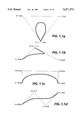
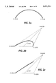
- FIGS. 1.1a through 1.1d and 2a through 2c are the curves used for the example analysis in Section 1.
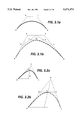
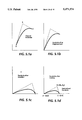
- FIG. 3.1a and 3.1b are an aid in the understanding of a cubic spline.
- FIG. 3.2b and 3.2b are an aid in the understanding of a conic.
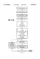
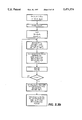
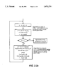
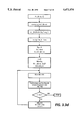
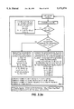
- FIGS. 3.3a through 3.3e are flowcharts of the algorithm to approximate a cubic spline by parabolic segments.
- FIG. 4 illustrates the approximation of a circular arc.
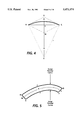
- FIG. 5 shows a parabolic trajectory
- FIGS. 5.1a through 5.1d show the steps involved in transforming an arbitrary parabola to a normalized parabola.
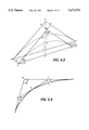
- FIG. 5.2 is an example of a parabola.
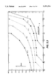
- FIG. 5.3 shows maximum skew as a function of included angle.
- FIG. 5.4 is the parabola defined in Section 5.4.
- FIGS. 5.5.1a through 5.5.1f illustrate the relationship between skew and included angle.
- FIG. 1 of this patent is a block diagram showing a graphic display system including a keyboard 1for inputting data, a graphic display unit 3, a graphic controller 4 for controlling the keyboard 1, and a computer 5. Described in this patent is a method of calculating curves from input data, normally in the form of page description language (PDL) and displaying the result on a raster output scanner in the form of said graphic display terminal.
- PDL page description language
- the first problem considered is the generation of a trajectory whose segments could be cubic splines, parabolas, conics, circular arcs and lines.
- the prevalent approach is to decompose the complex curves into line segments and then generate the line segments using a combination of general purpose computing elements and hardware accelerators.
- the decomposition of curves into line segments are generally done through a recursive sub division and test process until the approximation error is within the acceptable error limit.
- we give algorithms which decompose higher order curves into parabolic segments where the number of parabolic segments needed to approximate a curve to any desired level of accuracy can be determined a priori. This property is then used to set up simple stepper algorithms in software which directly generate the control points for the parabolic segments.
- parabolic trajectory can then be generated by a stepper hardware similar to that described by Marshall in Reference 1.
- Table 1.1 shows the advantage of decomposing curves into parabolic segments instead of line segments. For the examples considered the number of segments needed to approximate the curve can be reduced by factors of 3 to 9, if parabolic segments are used instead of linear segments.
- the different curves used for the example analysis along with their control points are shown in FIGS. 1.1 and 1.2.
- FIG. 1a-d are cubic splines
- FIG. 2a is a circular arc
- FIGS. 2b and c are conic sections. It is assumed that at most a single pixel error can be tolerated between the exact curve and its approximation.
- the second problem considered is the generation of a masked stroke with a center line trajectory whose segments could be cubic splines, parabolas, conics, circular arcs and lines.
- the prevalent approach is to decompose the trajectory into line segments and then compute the coordinates of a trapezoid corresponding to each line segment.
- This parazoid can then be filled to generate the masked stroke.
- a "parazoid” is a four sided figure in which the "parallel" sides are parabolas and the other two sides are lines.
- the following table shows the advantage of decomposing a masked stroke into parazoids instead of trapezoids.
- the number of parazoids needed to approximate a masked stroke can be between 1/3 to 1/9 of the number of trapezoids needed to approximate the same masked stroke.
- the different curves used for the example analysis along with their control points are shown in FIGS. 1.1 and 1.2. It is assumed that at most a single pixel error can be tolerated between the exact stroke and its approximation.
- Page Description Languages such as Interpress and Postscript support fairly powerful graphical primitives allowing the generation of filled areas whose outlines are defined by cubic splines, conics, parabolas, circular arcs and straight lines. Also they support strokes of specified widths whose center lines can be cubic splines, conics, parabolas, circular arcs and straight lines.
- PDL's Page Description Languages
- Interpress and Postscript support fairly powerful graphical primitives allowing the generation of filled areas whose outlines are defined by cubic splines, conics, parabolas, circular arcs and straight lines. Also they support strokes of specified widths whose center lines can be cubic splines, conics, parabolas, circular arcs and straight lines.
- Much of the paper deals with criteria for approximating higher order / difficult primitives by a sequence of lower order / simpler primitives. Some of the mathematical results may be of interest in their own right.
- section 3 the properties of cubic splines, parabolas, conic sections, circular arcs and straight lines are reviewed.
- parametric equations for each of these curves and the rules for the subdivision of these curves are given.
- a concise description of the algorithms are given in a flow chart form. The flow charts are given so that the essence of the algorithms are stated without complicating the flow charts. Several additional optimizations can be done at the time of coding these algorithms. No attempt has been made here to explicitly state all those optimizations.
- Section 4 is restricted to the problem of generating outlines. While this is an important part of PDL decomposition, there is also a need for generation of strokes of a specified width whose center line can be any one of the curves mentioned earlier.
- the strokes are obtained by stepping a filled elliptical pen along the center line.
- Liu has used the technique of stepping an elliptical pen to generate the outline of the stroke and then fill the enclosed region through a filling algorithm.
- This algorithm can be used to generate the outline of the stroke directly as a sequence of synthetic curves without the need for stepping an elliptical pen along the center line.
- a cubic spline with control points [A,B,C,D] can be described by the following parametric equation,
- FIG. 3.1 helps in understanding the definition and properties of a cubic spline.
- a cubic spline is shown defined by control points A, B, C, D.
- the curve is tangential to AB at A and CD at D.
- the cubic spline A, B, C, D subdivides into two cubic splines A, U, V, W and W, X, Y, D.
- a cubic spline [A,B,C,D] has the property that any segment of it is also a cubic spline. In particular it can be subdivided into two cubic splines whose control points are given by the following expressions.
- a conic with control points [A,B,C] and a shape parameter " ⁇ ", where 0 ⁇ 1 can be described by the following parametric equation.
- FIG. 3.2 helps in understanding the definition and properties of a conic.
- the conic of FIG. 3.2a is defined by control points A, B, C, and the conic of FIG. 3.2b A, B, C subdivides into two conics A, W, X and X, Y, C.
- a conic [A,B,C] has the property that any segment of it is also a conic. In particular it can be subdivided into two conics whose control points are given by the following expressions
- a parabola [A,B,C] has the property that any segment of it is also a parabola. In particular it can be subdivided into two parabolas whose control points are given by the following expressions.
- a parabola is also a special case of a cubic spline. In fact it is a quadratic spline. In a later section we will derive how both conics and cubic splines can be approximated by a sequence of adjoining parabolas.
- a circular arc with control points [A,B,C] is also a special case of a conic with the constraint that B lies on the perpendicular bisector of the side AC and has a shape parameter " ⁇ " given by the following equation.
- a circular arc may also be specified by the points [P,Q,R] with the arc starting at P passing through Q and ending at R. Later on we will show how control points [A,B,C] along with the parameter ⁇ can be derived from [P,Q,R].
- a straight line segment with control points [A,B] starts at A and ends at B and can be described by the following parametric equation.
- the flow charts 3.3a through 3.3c give the algorithms for decomposing Cubic Splines, Circular Arcs and Conics into parabolic segments.
- Flow chart 3.3d gives an algorithm for decomposing Parabolas into line segments.
- Flow chart 3.e gives an algorithm to split parabolas into sub parabolas, if necessary, and then generate parazoids.
- d is the distance between adjacent pixels in the coordinate system and m is the number of parabolic segments needed to approximate the cubic spline S.
- m 16
- c 0 cos 22.5
- c 2 sin 22.5
- c 3 tan 11.25.
- d is the distance between adjacent pixels in the coordinate system
- m is the number of linear segments needed to approximate the parabola P.
- a cubic spline S with control points [A,B,C,D] can be approximated by a parabola P with control points [A,(3B+3C-A-D)/4,D] with difference d between the two curves as a function of a defined error vector "e" as follows. ##EQU1##
- the maximum error is a simple function of the original control points [A,B,C,D]. If the maximum error is within the tolerance limits such as the spacing between adjacent pixels, then the approximation is acceptable. To simplify the computation a stricter constraint can be imposed if we replace e by (e x ⁇ e y )in the above expression.
- S 1 is also a cubic spline. It has control points [A 1 , B 1 , C 1 , D 1 ] as given below.
- d 1 is only a function of " ", the "length” of the segment along the "t” axis of the original spline and not a function of "x" the starting point of the segment. Since d 1 is a cubic function of , the process of approximating cubic spline segments by parabolas converges rapidly. Hence, for any desired level of accuracy, the number of segments "n" ( ⁇ 1/ ) needed for approximation by parabolas can be determined apriori without going through the subdivision process. Note that there is no loss of generality by making for each segment to be the same. For computational purposes it may be advantageous to make "n” a power of two.
- a parabola P with control points [A,E,D] can be approximated by a straight line L with control points [A,D] with difference d between the two curves as a function of a defined error vector "e" as follows. ##EQU5##
- P 1 is also a parabola which can be approximated by a straight line L 1 with control points [A 1 ,D 1 ] with the difference d 1 between the curves as a function of a defined error vector "e.sub. " as follows.
- d 1 is only a function of " ", the "length” of the segment along the "t” axis of the original parabola and not a function of "x" the starting point of the segment. Since d 1 is a quadratic function of , the process of approximating parabolic segments by straight lines also converges rapidly, though not as fast as the process of approximating cubic spline segments by parabolas. Hence, for any desired level of accuracy, the number of segments "n" ( ⁇ 1/ ) needed for approximation by straight lines can be determined apriori without going through the subdivision process. Note that there is no loss of generality by making for each segment to be the same. For computational purposes it may be advantageous to make n a power of two.
- a conic N with control points [A,B,C] can be approximated by a parabola P with control points [A,B,C] with difference d between the two curves given by the following expression ##EQU8##
- N 1 (t) and N 2 (t) denote the subconics of N(t) after subdivision.
- control points and shape parameters " ⁇ 1" and " ⁇ 2" for N 1 and N 2 are given by the following expressions.
- N 1 can be approximated by a parabola P 1 defined by
- N 2 can be approximated by a parabola P 2 defined by
- Table 4.1 gives the difference between the exact and approximate values of ⁇ 1 and ⁇ 2 for different values of ⁇ when the above formula is used.
- Table 4.2 gives the maximum error for different values of " ⁇ " when a circle of radius "r” is approximated by a parabola. The table also gives the maximum radius of the circle if we limit the error to 1 pixel.
- each sub arc can be directly replaced by a parabola and be within the acceptable error for all resolutions and radii of interest.
- a subtending angle of 22.5 degrees would also be an acceptable and probably a preferable choice.
- Interpress and Postscript allow the definition of trajectories which can be thickened to draw a masked stroke on paper.
- the trajectory itself can be made up of lines, arcs, conics, parabolas and cubic splines. It should be noted that in general, a curve that is parallel to another curve can only be represented by a higher order mathematical equation than the original one. Most of the implementations of masked stroke to date accomplish this by decomposing all the curves into line segments and then filling a sequence of trapezoids whose center lines are the decomposed line segments. In addition to the computation involved in decomposing the curves into lines, significant amount of computation has to be done to compute the vertices of each of the trapezoids.
- the amount of computation needed is directly proportional to the number of line segments needed for the approximation.
- Jack Liu in his paper gives a method by which the inner and outer trajectories of a thickened parabola can be approximated by a sequence of parabolas themselves. Since cubic splines, circular arcs and conics can be decomposed into a small number of parabolic segments (as shown in section 3), the masked stroke can then be implemented by filling a closed trajectory of parabolas and lines.
- FIG. 5 shows a parabolic trajectory WXY.
- Trajectories BCD and EFA are curves that are parallel to WXY and the trajectory ABCDEFA defines a region which if filled will generate the masked stroke for the curve WXY. Note that BCD and EFA are not parabolas in general.
- FIG. 5.1 shows the steps involved in transforming an arbitrary parabola to a normalized parabola. Note that the shape of the parabola is not distorted after this normalization process.
- a normalized parabola can therefore be completely defined by two parameters (B x , B y ) as opposed to six parameters (A x , A y , B x , B y , C x , C y ) needed for the original parabola.
- the parameters (k, ⁇ ) where k (later referred to as the skew) is the ratio of the lengths of the sides AB and AC and ⁇ is the included angle ABC.
- k is the skew parameter. It can be verified that (k, ⁇ ) and (B x , B y ) are related by the following equations.
- Table 5.3.3 presents the data of Table 5.3.2 and Table 5.3.1 in a different way. It lists the maximum tolerable skew (k) for either of the parallel curves as function of ⁇ (the included angle) and the maximum acceptable error limit.
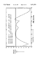
- FIG. 5.3.1 depicts the same data in a graphical form on a logarithmic scale.
- ⁇ is the angle between vectors BA and BC
- ⁇ 1 is the angle between vectors DA and DF
- ⁇ 2 is the angle between vectors FD and FC
- section 5.4 we developed a theory regarding how a parabola should be sub divided in order that the curves that are parallel to it can be approximated by parabolas themselves. We also derived results that enable us to calculate fairly easily the properties of the component parabolas in terms of the properties of the original parabola.
- section 5.2 we tabulated the maximum errors that will be observed by the use of the approximation process mentioned. In this section, we provide a simple but empirically derived criterion that can be used to test whether a parabola should be further sub divided or not. We also tabulate the maximum error that will be observed, if this test criterion is used.
- test criterion was chosen based upon three desirable qualities as listed below:
- ⁇ and k are the included angle and skew respectively for a given parabola as defined earlier, then the following test can be used to determine whether the parabola should be sub divided. Any time a parabola is sub divided it is done at the point given by the equation 5.4.14.
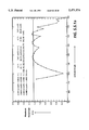
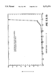
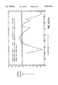
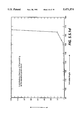
- FIGS. 5.5.1 a through f show a plot of the actual maximum error as a function of the included angle, if the limit for k is chosen according to the equations given above. The three plots correspond to the three cases where the designed maximum error limit was chosen to be 1.25%, 2.5% and 5.0% respectively. The figures also show a plot of k as a function of included angle.
Abstract
Description
              TABLE 1.2
______________________________________
         300 spi          600 spi
                    number           number
           number   of        number of
           of       trapezoid of     trapezoid
Curve Type parazoids
                    s         parazoids
                                     s
______________________________________
Cubic Spline 1
           6        32        7      56
Cubic Spline 2
           8        32        10     44
Cubic Spline 3
           5        32        6      40
Cubic Spline 4
           4        17        5      25
Circular Arc
           6        18        6      25
Conic 1    4        24        4      32
Conic 2    9        36        9      52
______________________________________
[X(t),Y(t)]=A(1-t).sup.3 +3Bt(1-t).sup.2 +3Ct.sup.2 (1-t)+Dt.sup.3
where 0<t<1 and A=[A.sub.x, A.sub.y ],B=[B.sub.x,B.sub.y ],C=[C.sub.x,C.sub.y ],D=[D.sub.x, D.sub.y ]
[X(t),Y(t)]=D.sub.0 +3D.sub.1 t+3D.sub.2 t.sup.2 +D.sub.3 t.sup.3 where 0<t<1
and D.sub.0 =A,D.sub.1 =B-A,D.sub.2 =C-2B+A, D.sub.3 =D-3C+3B-A
[A,(A+B)/2,(A+2B+C)/4,(A+3B+3C+D)/8]
[(A+3B+3C+D)/8,(B+2C+D)/4,(C+D)/2,D ]
(q+ρcos t)[X(t),Y(t)]=[(A+C)/2]q-[(A-C)/2]q sin t+pB cos t
where -π/2<t<π/2,q=1-ρ and A=[A.sub.x, A.sub.y ],B=[B.sub.x B.sub.y ],C=[C.sub.x,C.sub.y ]]
[A,(qA+ρB),q(A+C)/2+ρB)]
[q(A+C)/2+ρB),(qC+ρB),C ]
ρ'=1/[1+√(2-2ρ)]
[X(t),Y(t)]=A(1-t).sup.2 +2Bt(1-t)+Ct.sup.2
where 0<t<1 and A=[A.sub.x,A.sub.y ],B=[B.sub.x,B.sub.y ],C=[C.sub.x,C.sub.y ]]
[X(t),Y(t)]=D.sub.0 +2.sub.D.sub.1 t+D.sub.2 t.sup.2 where 0<t<1
and D.sub.0 =A,D.sub.1 =B-A,D.sub.2 =C-2B+A
[A,(A+B)/2,(A+2B+C)/4]
[(A+2B+C)/4,(B+C)/2,C ]
ρ=m[√(1+m.sup.2)]-m.sup.2, where m=tan ABC/2
[X(t),Y(t)]=A(1-t)+Bt where 0<t<1,A =[A.sub.x,A.sub.y ] and B=[B.sub.x,B.sub.y ]
[S(t)]=A+3(B-A)t+3(C-2B+A)t.sup.2 +(D-3C+3B-A)t.sup.3
[P(t)]=A+2(E-A)t+(D-2E+A)t.sup.2
D-3C+3B-A=0,D-2E+A=3(C-2B+A) and 2(E-A)=3(B-A)
D-3C+3B-A=0,E=(3B+3C-A-D)/4
[S.sub.1 (u)]=X.sub.0 +3X.sub.1 (x+δu)+3X.sub.2 (x+δu).sup.2 +X3(x+δu).sup.3
for 0<u<1 where
X.sub.0 =A,X.sub.1 =(B-A),X.sub.2 =(C-2B+A),X.sub.3 =(D-3C+3B-A)
[S.sub.1 (u)]=Y.sub.0 +3Y.sub.1 u+3Y.sub.2 u.sup.2 +Y.sub.3 u.sup.3
for 0<u<1 where
Y.sub.0 =A+3(B-A)x+3(C-2B+A)x.sup.2 +(D-3C+3B-A)x.sup.3
Y.sub.1 =[(B-A)+2(C-2B+A)x+(D-3C+3B-A)x.sup.2 ]δ
Y.sub.2 =[(C-2B+A)+(D-3C+3B-A)x]δ.sup.2
Y.sub.3 =(D-3C+3B-A)δ.sup.3
A.sub.1 Y.sub.0,B.sub.1 =Y.sub.1 +Y.sub.0,C.sub.1 =(Y.sub.2 +2Y.sub.1 +Y.sub.0),D.sub.1 =(Y.sub.3 +3Y.sub.2 +3Y.sub.1 +Y.sub.0)
E.sub.1 =(4Y.sub.0 +6Y.sub.1 -Y.sub.3)/4
E.sub.1 =S(x)+S'(x)δ/2-S'"(x)δ.sup.3 /24.
d.sub.1 (u)=[S.sub.1 (u)-P.sub.1 (u)]=-(e.sub.1 /2)[2u.sup.3 -3u.sup.2 +u]where e.sub.1 =3C.sub.1 -3B.sub.1 -D.sub.1 +A.sub.1
[P(t)]=A+2(E-A)t+(D-2E+A)t.sup.2
[L(t)]=A+(D-A)t
D-2E+A=0 and 2(E-A)=(D-A)
D-2E+A=0
[P.sub.1 (u)]=A.sub.1 +2(E.sub.1 -A.sub.1)u+(D.sub.1 -2E.sub.1 +A.sub.1)u.sup.2
for 0<u<1 where
A.sub.1 =A+2(E-A)x+(D-2E+A)x.sup.2
E.sub.1 =A+[(E-A)+(D-2E+A)x]δ
D.sub.1 =2E.sub.1 -A.sub.1 +(D-2E+A)δ.sup.2
d.sub.1 (u)=[S.sub.1 (u)-P.sub.1 (u)]=e.sub.1 [u.sup.2 -u]
where e.sub.1 =(D.sub.1 -2E.sub.1 +A.sub.1)=(D-2E+A)δ.sup.2
(q+ρ cos t)N(t)]=[(A+C)/2]q-[(A-C)/2]q sin t+ρB cos t
where -π/2<t<π/2 and q=1-ρ
(1+cos t)P(t)]=[(A+C)/2]-[(A-C)/2]sin t+B cos t
where -π/2<t<π/2
[P(u)]=A+2(B-A)u+(C-2B+A)u.sup.2 where 0<u<1
q=ρ=0.5
[A,(qA+ρB),q(A+C)/2+ρB)] for N.sub.1
[q(A+C)/2+ρB),(qC+ρB),C] for N.sub.2
ρp.sub.1 =ρ.sub.2 =1/[1+√2(1-ρ)]
[P.sub.1 (u)]=A.sub.1 +2(C.sub.1 -A.sub.1)u+(C.sub.1 -2B.sub.1 +A.sub.1)u.sup.2
for 0<u<1 where
A.sub.1 =A,B.sub.1 =(qA+ρB),C.sub.1 =q(A+C)/2+ρB)
|d.sub.1 |.sub.max +|e.sub.1 |(1-2ρ.sub.1)/4 where e.sub.1 =C.sub.1 -2B.sub.1 +A.sub.1
[P.sub.2 (u)]=A.sub.2 +2(C.sub.2 -A.sub.2)u+(C.sub.2 -2B.sub.2 +A.sub.2)u.sup.2
for 0<u<1 where
A.sub.2 =q(A+C)/2+ρB,B.sub.2 =(qC+ρB),C.sub.1 =C
|d.sub.2 |.sub.max =|e.sub.2 |(1-2ρ.sub.2)/4 where e.sub.2 =C.sub.2 -2B.sub.2 +A.sub.2
ρ.sub.1 =ρ.sub.2 ≈0.5-δ/4
|d|.sub.max =|e|δ/2
|d.sub.1 |.sub.max ≈|d.sub.2 |.sub.max ≈|e|δ/32=|d|.sub.max /16
              TABLE 4.1
______________________________________
            Approximation
       p    error
______________________________________
       0.2  7.7 × 10.sup.-4
       0.25 2.7 × 10.sup.-4
       0.3  3.9 × 10.sup.-5
       0.35 3.0 × 10.sup.-5
       0.4  2.4 × 10.sup.-5
       0.45 5.3 × 10.sup.-6
       0.5  0.0
       0.55 1.1 × 10.sup.-5
       0.6  1.0 × 10.sup.-4
       0.65 4.9 × 10.sup.-4
       0.7  1.7 × 10.sup.-3
______________________________________
(q+ρcos t)R(t)]=[(A+C)/2]q-[(A-C)/2]q sin t+ρB cos t
where -π/2<t<π/2 and q=1-ρ
[P(u)]=A+2(B-A)u+(C-2B+A)u.sup.2 where 0<u<1
(2+2 cos t-2ρ sin.sup.2 t)d(t)=(q-ρ)[(C-2B+A)+(C-A) sin t] cos t
              TABLE 4.2
______________________________________
                   max. radius in
                                max. radius in
       maximum error
                   inches at 300 spi.
                                inches at 600 spi.
θ in
       due to parabolic
                   for less than one
                                for less than one
degrees
       approximation
                   pixel error  pixel error
______________________________________
15.0   3.7 × 10.sup.-5 r
                   90.09        45.05
22.5   1.9 × 10.sup.-4 r
                   17.71        8.85
30.0   6.0 × 10.sup.-4 r
                   5.55         2.78
45.0   3.1 × 10.sup.-3 r
                   1.08         0.54
60.0   1.0 × 10.sup.-2 r
                   0.33         0.17
______________________________________
k=(B.sub.x.sup.2 +B.sub.y.sup.2)/([1-B.sub.x.sup.2 ]+B.sub.y.sup.2) 5.1.1
cos θ=(B.sub.x.sup.2 +B.sub.y.sup.2 -B.sub.x)/√{(B.sub.x.sup.2 +B.sub.y.sup.2)([1-B.sub.x.sup.2)]+B.sub.y.sup.2)} 5.1.2.
B.sub.x =(k.sup.2 -k cosθ)/(1+k.sup.2 -2k cos θ) 5.1.3
B.sub.y =(sin θ)/(1+k.sup.2 -2k cos θ) 5.1.4
D=A+d[-sin θ.sub.1,cos θ.sub.1 ] 5.2.1.
E=B-d[(cos θ.sub.1 +cos θ.sub.2),(sin θ.sub.1 +sin θ.sub.2)]/sin(θ.sub.1 -θ.sub.2) 5.2.2.
F=C+d[sin θ.sub.2, -cos θ.sub.2 ] 5.2.3.
sin θ.sub.1 =(B.sub.y -A.sub.y)/|AB|, cos θ.sub.1 =(B.sub.x -A.sub.x)/|AB| 5.2.4
sin θ.sub.2 =(B.sub.y -C.sub.y)/|BC|,cos θ.sub.2 =(B.sub.x -C.sub.x)/|BC| 5.2.5
T=(C+2B+A)/4 and U+(F+2E+D)/4 5.2.6
U.sub.x -T.sub.x =d[sin θ.sub.2 -sin θ.sub.1 -2(cos θ.sub.1 +cos θ.sub.2)/sin (θ.sub.1 -θ.sub.2)]/4 5.2.6.
U.sub.y -T.sub.y =d[cos θ.sub.1 -cos θ.sub.2 -2(sin θ.sub.1 +sin θ.sub.2)/sin(θ.sub.1 -θ.sub.2)]/4 5.2.8
|UT|=(d/2)([sin θ/2]+1/[sin θ/2]) 5.2.9
E=B+d[(-sin θ.sub.1 +cos θ.sub.1 cot θ/2),(cos θ.sub.1 +sin θ.sub.1 cot θ/2)] 5.2.10
              TABLE 5.3.1
______________________________________
k =       k =
1         2      k = 4   k = 8 k = 16
                                     k = 32
                                           k = 64
______________________________________
θ = 90
       6.07   2.36   10.40 25.33 40.41 53.40 --
θ = 100
       3.57   0.85   8.77  20.45 32.52 43.17 51.60
θ = 110
       2.00   0.69   7.08  15.95 25.28 33.72 40.56
θ = 120
       1.04   0.77   5.43  11.90 18.83 25.21 30.48
θ = 130
       0.48   0.71   3.91  8.38  13.23 17.78 21.61
θ = 140
       0.19   0.55   2.57  5.42  8.55  11.53 14.07
θ = 150
       0.06   0.35   1.48  3.08  4.85  6.55  8.03
θ = 160
       0.01   0.17   0.67  1.38  2.17  2.94  3.62
θ = 170
       0.00   0.04   0.17  0.35  0.55  0.74
______________________________________
 Maximum Percentage error observed when outer parallel curve is
 approximated by another parabola
              TABLE 5.3.2
______________________________________
k =       k =
1         2      k = 4   k = 8 k = 16
                                     k = 32
                                           k = 64
______________________________________
θ = 90
       6.07   2.26   11.02 26.98 43.72 --    --
θ = 100
       3.57   0.79   9.19  21.56 34.77 56.45 --
θ = 110
       2.00   0.74   7.35  16.67 26.76 36.36 --
θ = 120
       1.04   0.80   5.60  12.35 19.74 26.86 --
θ = 130
       0.48   0.73   4.00  8.63  13.75 24.60 --
θ = 140
       0.19   0.56   2.62  5.55  8.82  12.01 69.71
θ = 150
       0.06   0.35   1.50  3.13  4.96  6.76  9.75
θ = 160
       0.01   0.17   0.67  1.39  2.20  3.00  3.72
θ = 170
       0.00   0.04   0.17  0.35  0.55  0.75
______________________________________
 Maximum Percentage error observed when inner parallel curve is
 approximated by another parabola
                                  TABLE 5.3.3
__________________________________________________________________________
error limit = 1%
              error limit = 2%
                       error limit = 4%
                                error limit = 8%
                                         error limit = 16%
__________________________________________________________________________
θ = 90
     k = 1.000
              k = 1.000
                       k = 1.000
                                k ≦ 3.438
                                         k ≦ 5.000
θ = 100
     k = 1.000
              k = 1.000
                       k ≦ 2.797
                                k ≦ 3.719
                                         k ≦ 5.938
θ = 110
     k = 1.000
              k ≦ 2.375
                       k ≦ 2.969
                                k ≦ 4.219
                                         k ≦ 7.625
θ = 120
     k = 1.000
              k ≦ 2.484
                       k ≦ 3.281
                                k ≦ 5.188
                                         k ≦ 11.25
θ = 130
     k ≦ 2.156
              k ≦ 2.750
                       k ≦ 3.984
                                k ≦ 7.250
                                         k ≦ 22.00
θ = 140
     k ≦ 2.406
              k ≦ 3.375
                       k ≦ 5.625
                                k ≦ 13.50
                                         k ≦ 63.83
θ = 150
     k ≦ 3.094
              k ≦ 5.000
                       k ≦ 1.00
                                k ≦ 49.88
                                         k ≦ 256.0*
θ = 160
     k ≦ 5.625
              k ≦ 13.50
                       k ≦ 88.
                                k ≦ 256.0*
                                         k ≦ 256.0*
θ = 170
     k ≦ 88.00
              k ≦ 256.0*
                       k ≦ 256.0*
                                k ≦ 256.0*
                                         k ≦ 256.0*
__________________________________________________________________________
 *Maximum acceptible skew when either of the parallel curves is
 approximated by a parabola
              TABLE 5.3.4
______________________________________
Included
        Included angle
                    Included angle
                                Included angle
angle for
        after sub   after sub   after sub
the original
        dividing into
                    dividing into
                                dividing into
Parabola
        two parabolas
                    four parabolas
                                eight parabolas
______________________________________
 90     135         157.5       168.75
100     140         160.0       170.00
110     145         162.5       171.25
120     150         165.0       172.50
130     155         167.5       173.75
______________________________________
k+l.sub.1 /l.sub.2 where l.sub.1 =|AB|and l.sub.2 =|AC| 5.4.1
k.sub.1 =l.sub.3 /l.sub.4 where l.sub.3 =|AD|and l.sub.4 =|DE| 5.4.2
k.sub.2 =l.sub.5 /l.sub.6 where l.sub.5 =|EF|and l.sub.6 =|FC| 5.4.3
(180-θ.sub.1)+(180 -θ.sub.2)=180-θ 5.4.4
if θ.sub.1 θ.sub.2 then θ.sub.1 =θ.sub.2 =π+θ/2 5.4.5
if θ<180 then 90+θ/2>θ 5.4.6
cos φ=(V.sub.1x V.sub.2x +V.sub.1y V.sub.2y)/(|V.sub.1 ||V.sub.2 |) 5.4.7.
D=A+(B-A)u,E=A+2(B-A)u+(C-2B+A)u.sup.2 and F=C+(B-C)(1-u) 5.4.8
cos θ=[(A.sub.x -B.sub.x)(C.sub.x -B.sub.x)+(A.sub.y -B.sub.y)(C.sub.y -B.sub.y)]/l.sub.1 l.sub.2 5.4.9
cos θ.sub.1 =[(A.sub.x -D.sub.x)(F.sub.x-D.sub.x)+(A.sub.y -D.sub.y)(F.sub.y -D.sub.y)]/[|DA||DF|]5.4.10
cos θ.sub.2 =[(D.sub.x -F.sub.x)(C.sub.x -F.sub.x)+(D.sub.y -F.sub.y)(C.sub.y -F.sub.y)]/[|DF||FC|]5.4.11
|DA|=ul.sub.1 and |FC|=(1-u)l.sub.2 5.4.12
A-D=(A-B)u 5.4.13
F-D=(C-B)u+(B-A)(1-u) 5.4.14
C-F=(C-B)(1-u) 5.4.15
cos θ.sub.1 =[-l.sub.1.sup.2 u(1-u)+l.sub.1 l.sub.2 u.sup.2 cos θ]/ul.sub.1 |DF| 5.4.16
cos θ.sub.2 =[-l.sub.2.sup.2 u(1-u)+l.sub.1 l.sub.2 (1-u).sup.2 cos θ]/(1-u)l.sub.2 |DF| 5.4.17
|DE|.sup.2 =(D.sub.x -E.sub.x).sup.2 +(D.sub.y -E.sub.y).sup.2 5.4.19
|DE|.sup.2 =[(B.sub.x -A.sub.x)(u-u.sup.2)+(C.sub.x -B.sub.x)u.sup.2].sup.2 +[(B.sub.y -A.sub.y)(u-u.sup.2)+(C.sub.y -B.sub.y)u.sup.2 ].sup.2 5.4.20
|DE|.sup.2 =[u.sup.2 (1-u).sup.2 l.sub.1.sup.2 +u.sup.4 l.sub.2.sup.2 +2u.sup.3 (1-u)[(B.sub.x -A.sub.x)(C.sub.x -B.sub.x)+(B.sub.y A.sub.y)(C.sub.y -B.sub.y)]] 5.4.21
|DE|.sup.2 =[u.sup.2 (1-u).sup.2 l.sub.1.sup.2 +u.sup.4 l.sub.2.sup.2 -2u.sup.3 (1-u)l.sub.1 l.sub.2 cos θ] 5.4.22
-0.391>cos θ>-0.843: 1/(-0.11-3.61 cosθ))<k<(-0.11-3.61 cos θ)
-0.843>cos θ>-0.940: 1/(-21.00-28.25 cos θ)<k<(-21.00-28.25 cos θ))
-0.940>cos θ>-0.980: 1/(-334.76-362.00 cos θ))<k<(-334.76-362.00 cos θ))
-0.980>cos θ>-1.000: 0<k<∞
-0.340>cos θ)>-0.891: 1/(-1.19-6.75 cos θ)<k<(-1.19-6.75 cos θ)
-0.891> cos θ>-0.965: 1/(-160.50-187.50 cosθ)<k<(-160.50-187.50 cos θ)
-0.965>cos θ>-1.000: 0<k<∞
-0.010>cos θ>-0.710: 1/(1.70-4.20 cos θ)<k<(1.70-4.20 cos θ))
-0.710> cos θ>-0.874: 1/(-21.50-37.00 cos θ)<k=(-21.50-37.00 cos θ)
-0.874> cos θ>-0.950: 1/(-880.00-1020.00 cos θ))<k<(-880.00-1020.00 cos θ)
-0.950> cos θ>-1.000: <k<∞
Claims (2)
Priority Applications (1)
| Application Number | Priority Date | Filing Date | Title |
|---|---|---|---|
| US08/297,746 US5471574A (en) | 1990-06-14 | 1994-08-29 | Method for displaying a computer generated graphic on a raster output scanner |
Applications Claiming Priority (3)
| Application Number | Priority Date | Filing Date | Title |
|---|---|---|---|
| US53795190A | 1990-06-14 | 1990-06-14 | |
| US13622693A | 1993-10-13 | 1993-10-13 | |
| US08/297,746 US5471574A (en) | 1990-06-14 | 1994-08-29 | Method for displaying a computer generated graphic on a raster output scanner |
Related Parent Applications (1)
| Application Number | Title | Priority Date | Filing Date |
|---|---|---|---|
| US13622693A Continuation-In-Part | 1990-06-14 | 1993-10-13 |
Publications (1)
| Publication Number | Publication Date |
|---|---|
| US5471574A true US5471574A (en) | 1995-11-28 |
Family
ID=26834136
Family Applications (1)
| Application Number | Title | Priority Date | Filing Date |
|---|---|---|---|
| US08/297,746 Expired - Fee Related US5471574A (en) | 1990-06-14 | 1994-08-29 | Method for displaying a computer generated graphic on a raster output scanner |
Country Status (1)
| Country | Link |
|---|---|
| US (1) | US5471574A (en) |
Cited By (10)
| Publication number | Priority date | Publication date | Assignee | Title |
|---|---|---|---|---|
| US5615324A (en) * | 1994-03-17 | 1997-03-25 | Fujitsu Limited | Distributed image processing apparatus |
| WO1998032319A2 (en) * | 1997-01-13 | 1998-07-30 | Laser Products, Inc. | Method for generating curves |
| US5978512A (en) * | 1997-01-21 | 1999-11-02 | Daewoo Electronics Co., Ltd | Polygonal approximation method and apparatus for use in a contour encoding system |
| US5986658A (en) * | 1997-01-31 | 1999-11-16 | Hewlett-Packard Co. | Method and apparatus for raster computer graphics display of rotation invariant line styles |
| US5995902A (en) * | 1997-05-29 | 1999-11-30 | Ag-Chem Equipment Co., Inc. | Proactive swath planning system for assisting and guiding a vehicle operator |
| US6266065B1 (en) * | 1998-03-02 | 2001-07-24 | Industrial Technology Research Institute | Method for rendering 3D triangle primitives |
| US20040121829A1 (en) * | 2002-12-23 | 2004-06-24 | Nintendo Software Technology Corporation | Method and apparatus for modeling a track in video games using arcs and splines that enables efficient collision detection |
| US20060197759A1 (en) * | 2001-12-12 | 2006-09-07 | Technoguide As | Three dimensional geological model construction |
| US20080005212A1 (en) * | 2006-05-22 | 2008-01-03 | Levien Raphael L | Method and apparatus for interactive curve generation |
| US20090237410A1 (en) * | 2008-03-20 | 2009-09-24 | Dick Baardse | System and method for offset curves with bidirectional constraints |
Citations (1)
| Publication number | Priority date | Publication date | Assignee | Title |
|---|---|---|---|---|
| US4829456A (en) * | 1985-06-07 | 1989-05-09 | Hitachi, Ltd. | Three-dimensional surface display method |
-
1994
- 1994-08-29 US US08/297,746 patent/US5471574A/en not_active Expired - Fee Related
Patent Citations (1)
| Publication number | Priority date | Publication date | Assignee | Title |
|---|---|---|---|---|
| US4829456A (en) * | 1985-06-07 | 1989-05-09 | Hitachi, Ltd. | Three-dimensional surface display method |
Cited By (17)
| Publication number | Priority date | Publication date | Assignee | Title |
|---|---|---|---|---|
| US5615324A (en) * | 1994-03-17 | 1997-03-25 | Fujitsu Limited | Distributed image processing apparatus |
| US6014148A (en) * | 1994-08-17 | 2000-01-11 | Laser Products, Inc. | Method for generating two dimensional and three dimensional smooth curves and for driving curve forming devices |
| WO1998032319A2 (en) * | 1997-01-13 | 1998-07-30 | Laser Products, Inc. | Method for generating curves |
| WO1998032319A3 (en) * | 1997-01-13 | 1998-10-29 | Laser Products Inc | Method for generating curves |
| US5978512A (en) * | 1997-01-21 | 1999-11-02 | Daewoo Electronics Co., Ltd | Polygonal approximation method and apparatus for use in a contour encoding system |
| US5986658A (en) * | 1997-01-31 | 1999-11-16 | Hewlett-Packard Co. | Method and apparatus for raster computer graphics display of rotation invariant line styles |
| US5995902A (en) * | 1997-05-29 | 1999-11-30 | Ag-Chem Equipment Co., Inc. | Proactive swath planning system for assisting and guiding a vehicle operator |
| US6266065B1 (en) * | 1998-03-02 | 2001-07-24 | Industrial Technology Research Institute | Method for rendering 3D triangle primitives |
| US7542037B2 (en) * | 2001-12-12 | 2009-06-02 | Schlumberger Technology Corporation | Three dimensional geological model construction |
| US20060197759A1 (en) * | 2001-12-12 | 2006-09-07 | Technoguide As | Three dimensional geological model construction |
| US20040121829A1 (en) * | 2002-12-23 | 2004-06-24 | Nintendo Software Technology Corporation | Method and apparatus for modeling a track in video games using arcs and splines that enables efficient collision detection |
| US8784171B2 (en) * | 2002-12-23 | 2014-07-22 | Nintendo Co., Ltd. | Method and apparatus for modeling a track in video games using arcs and splines that enables efficient collision detection |
| US20080005212A1 (en) * | 2006-05-22 | 2008-01-03 | Levien Raphael L | Method and apparatus for interactive curve generation |
| US8520003B2 (en) * | 2006-05-22 | 2013-08-27 | Raphael L Levien | Method and apparatus for interactive curve generation |
| US8810579B2 (en) | 2006-05-22 | 2014-08-19 | Raphael L. Levien | Method and apparatus for interactive curve generation |
| US9230350B2 (en) | 2006-05-22 | 2016-01-05 | Raphael L. Levien | Method and apparatus for interactive curve generation |
| US20090237410A1 (en) * | 2008-03-20 | 2009-09-24 | Dick Baardse | System and method for offset curves with bidirectional constraints |
Similar Documents
| Publication | Publication Date | Title |
|---|---|---|
| US5471574A (en) | Method for displaying a computer generated graphic on a raster output scanner | |
| US7212205B2 (en) | Curved surface image processing apparatus and curved surface image processing method | |
| US20090027396A1 (en) | Method for fitting a parametric representation to a set of objects | |
| WO1984002993A1 (en) | Method and apparatus for representation of a curve of uniform width | |
| JP3287685B2 (en) | Data conversion device and method | |
| Bajaj et al. | A-splines: local interpolation and approximation using Gk-continuous piecewise real algebraic curves | |
| Szilvási-Nagy et al. | Generating curves and swept surfaces by blended circles | |
| US5422990A (en) | Bezier spline to quadratic polynomial fragment conversion | |
| Kilgard | Polar stroking: new theory and methods for stroking paths | |
| Jiang et al. | Square root 3-Subdivision Schemes: Maximal Sum Rule Orders | |
| Fang | G3 approximation of conic sections by quintic polynomial curves | |
| US20050168462A1 (en) | Method and apparatus for generating m-degree forms in a n-dimension space | |
| Liang et al. | Properly posed sets of nodes for multivariate Lagrange interpolation in Cs | |
| EP0461919A2 (en) | Data processing apparatus | |
| US7333109B2 (en) | System, method and computer program product for modeling at least one section of a curve | |
| Bajaj et al. | Regular algebraic curve segments (III)—applications in interactive design and data fitting | |
| EP0461916A2 (en) | Displaying computer-generated images using rapid decomposition of outlines | |
| Rice | Spatial bounding of self-affine iterated function system attractor sets | |
| Zhu et al. | C2 interpolation T-splines | |
| Bihan | Asymptotic behaviour of Betti numbers of real algebraic surfaces | |
| Matschke | On the square peg problem and its relatives | |
| Kitazawa | Explicit smooth real algebraic functions which may have both compact and non-compact preimages on smooth real algebraic manifolds | |
| Bachman et al. | Cohomology fractals, Cannon–Thurston maps, and the geodesic flow | |
| Karu | Toric residue mirror conjecture for Calabi-Yau complete intersections | |
| Hecklin et al. | Local Lagrange interpolation with cubic C1 splines on tetrahedral partitions |
Legal Events
| Date | Code | Title | Description |
|---|---|---|---|
| AS | Assignment |
Owner name: XEROX CORPORATION, CONNECTICUT Free format text: ASSIGNMENT OF ASSIGNORS INTEREST;ASSIGNOR:PRASAD, BINDIGANAVELE;REEL/FRAME:007185/0307 Effective date: 19940801 |
|
| FPAY | Fee payment |
Year of fee payment: 4 |
|
| AS | Assignment |
Owner name: BANK ONE, NA, AS ADMINISTRATIVE AGENT, ILLINOIS Free format text: SECURITY INTEREST;ASSIGNOR:XEROX CORPORATION;REEL/FRAME:013153/0001 Effective date: 20020621 |
|
| FPAY | Fee payment |
Year of fee payment: 8 |
|
| AS | Assignment |
Owner name: JPMORGAN CHASE BANK, AS COLLATERAL AGENT, TEXAS Free format text: SECURITY AGREEMENT;ASSIGNOR:XEROX CORPORATION;REEL/FRAME:015134/0476 Effective date: 20030625 Owner name: JPMORGAN CHASE BANK, AS COLLATERAL AGENT,TEXAS Free format text: SECURITY AGREEMENT;ASSIGNOR:XEROX CORPORATION;REEL/FRAME:015134/0476 Effective date: 20030625 |
|
| REMI | Maintenance fee reminder mailed | ||
| LAPS | Lapse for failure to pay maintenance fees | ||
| STCH | Information on status: patent discontinuation |
Free format text: PATENT EXPIRED DUE TO NONPAYMENT OF MAINTENANCE FEES UNDER 37 CFR 1.362 |
|
| FP | Lapsed due to failure to pay maintenance fee |
Effective date: 20071128 |
|
| AS | Assignment |
Owner name: XEROX CORPORATION, CONNECTICUT Free format text: RELEASE BY SECURED PARTY;ASSIGNOR:JPMORGAN CHASE BANK, N.A. AS SUCCESSOR-IN-INTEREST ADMINISTRATIVE AGENT AND COLLATERAL AGENT TO JPMORGAN CHASE BANK;REEL/FRAME:066728/0193 Effective date: 20220822 |