US20060226837A1 - Methods and apparatus for magnetic resonance imaging in inhomogeneous fields - Google Patents

Abstract

Methods for providing practical magnetic resonance imaging systems that utilize non-homogeneous background fields, B₀, as well as, possibly non-linear, gradient fields G₁, G₂ to make non-invasive measurements to determine, among other things, a spin density function. These methods are time and SAR efficient, using one or two refocusing pulses for each line measured in k-space. Two types of non-homogeneous background fields are considered: background fields B₀ in which the function |B₀| does not have a critical point within the field of view, and background fields B₀ such that the function |B₀| has a single critical point within the field of view. In the first case, an MR-imaging device may be constructed by using the permanent gradient in the background field, B₀, as a slice select gradient, so long as particular criteria are met. The methods demonstrate that there are many practical circumstances where these criteria can all be met. An apparatus meeting such criteria can allow one to make non-invasive measurements that allow a reconstruction of the spin density function determined by a 3-dimensional object. The measurement process using such an apparatus includes the steps of placing the object to be imaged in an inhomogeneous background field B₀ for a sufficient time for the nuclear spins of a desired species to be polarized, selectively exciting the polarized nuclear spins using standard selective excitation RF-pulse sequences from apparatus that generates substantially homogeneous RF-fields within a field of view of the apparatus, and spatially encoding phases of the excited nuclear spins using gradient fields G₁, G₂, where the functions |B₀|, <B₀, G₁>, <B₀, G₂> define coordinates within the field of view of the apparatus. Also, under these same assumptions on the magnetic fields, one can use a combination of the fields B₀, G₁, and G₂ to define a slice select direction not parallel to the permanent gradient in B₀ In this case one recovers a 2D-imaging protocol, using an inhomogeneous background field, with most of the features of standard spin-warp imaging. In the second case, magnets may be constructed so that |B₀| has an isolated non-zero local minimum. Using selective excitation, one can excite only the spins lying in a small neighborhood of this local minimum. In this way one can do spatially localized, high SNR, spectroscopic measurements, without any need for further spatial encoding.

Description

CROSS-REFERENCE TO RELATED APPLICATIONS
• This application claims benefit to U.S. Provisional Application Nos. 60/663,937 filed Mar. 21, 2005 (Attorney Docket No. UPN-4416) and 60/737,283 filed Nov. 16, 2005 (Attorney Docket No. UPN-4581).
GOVERNMENT SUPPORT
• The present invention was supported by the National Science Foundation under Grant Nos. NSF DMS99-70487, DMS02-07123, and DMS02-3705. The government may have certain rights in the invention.
FIELD OF THE INVENTION
• The present invention relates to methods and apparatus for obtaining magnetic resonance images in inhomogeneous magnetic fields and, more particularly, to imaging with a background field B₀ that varies both in magnitude and direction, both with and without critical points.
BACKGROUND OF THE INVENTION
• In the standard approach to magnetic resonance imaging one uses a strong background field that is as homogeneous as possible. Commercial MR imaging magnets are homogeneous, within the field of view, to about 1 ppm. In “open” MRI systems, the field homogeneity is somewhat less, but still in this general range. One can imagine a variety of situations where it might be useful to do magnetic resonance imaging with the object placed entirely outside the magnet's bore. As a consequence of Runge's Theorem, it is possible to design coils so that this external field is as homogeneous as one would like, in a given region of space. However, this requires a large expenditure of power and complicated, difficult to design arrangements of coils. On the other hand, with simpler arrangements of permanent magnets or electromagnets, one can produce a field, B₀, such that, in a given region of space, exterior to the magnets, or coils: (1) The field is strong; (2) The direction of B₀ varies in a small solid angle; (3) The level sets of |B₀| are smooth; and (4) The size of ∇|B₀| is not too large.
• Several groups have considered problems of this sort. Generally speaking, the prior art uses pulsed gradients for spatial encoding, and refocusing pulses to repeatedly refocus the accumulating phase in the direction of the permanent gradient. These ideas are described in U.S. Pat. No. 4,656,425 to Bendel, as well as in U.S. Pat. No. 5,023,554 to Cho and Wong. The idea is further developed by Crowley and Rose as described in U.S. Pat. No. 5,304,930 and U.S. Pat. No. 5,493,225. Pulsed gradients are also used in SPRITE, though for different reasons, as noted by Balcom et al., Single-point ramped imaging with T ₁ enhancement (SPRITE), J. Mag. Res. A, Vol. 123 (1996), pp. 131-134.
• Another group considering such problems is that of Dr. Alexander Pines at University of California at Berkeley. His work is described in the recent PNAS paper: “Three-dimensional phase-encoded chemical shift MRI in the presence of inhomogeneous fields” by Vasiliki Demas, Dimitris Sakellariou, Carlos A. Meriles, Songi Han, Jeffrey Reimer, and Alexander Pines. Their approach is somewhat different in that they try to match inhomogeneities in the B₁-field with that in the B₀-field in order to effectively “cancel” them out. Their efforts are more directed towards spectroscopy and they consider very small field gradients.
• Still another group working on problems of this sort is that of Bernhard Blümich at RWTH Aachen in Aachen, Germany. This group's work is described in “The NMR-mouse: construction, excitation, and applications” by Blümich B, Blumler P, Eidmann G, Guthausen A, Haken R, Schmitz U, Saito K, and Zimmer G in Magn Reson Imaging. 1998, pgs 479-484. Their approach is again different from what is described herein in that it uses a stroboscopic acquisition technique. Though it is very good for spectroscopy of materials, it is too time consuming and SAR intensive for in vivo applications.
• The present invention addresses methods and apparatus for imaging in such a field as described in a paper by one of the present inventors (C L Epstein) entitled “Magnetic Resonance Imaging in Inhomogeneous Fields,” Inverse Problems, Vol. 20, pages 753-780 (Mar. 19, 2004), the contents of which are hereby incorporated by reference in their entirety. Further refinements of this method are presented herein for acquiring data that lead to a fairly standard 2d-reconstruction problem.
SUMMARY OF THE INVENTION
• Methods are described for providing practical magnetic resonance imaging systems that utilize non-homogeneous background fields, B₀, as well as possibly non-linear basic gradient fields G₁, G₂ to make non-invasive measurements to determine, among other things, a spin density function. Generally, two types of non-homogeneous background fields are considered:
• • a. Background fields B₀ in which the function |B₀| does not have a critical point within the field of view.
  • b. Background fields B₀ such that the function |B₀| has a single critical point within the field of view.
• In the case of background fields B₀ without a critical point in the field of view, an MR-imaging device may be constructed by using the permanent gradient in the background field, B₀, as a slice select gradient, so long as:
• • a. the direction (as opposed to magnitude) of the background field does not vary too much within the field of view;
  • b. the strength of the background field remains large throughout the field of view so that the local Larmor frequency may be determined to a high degree of accuracy by the components of the various fields parallel to B₀;
  • c. the level sets of the function |B₀| within the field of view are expressible as graphs of smooth functions over a region lying in a plane;
  • d. apparatus can be constructed to generate magnetic fields G₁, G₂ so that the functions |B₀|, <B₀, G₁>, <B₀, G₂> define coordinates within the field of view;
  • e. for parameters (η₁, η₂) lying in a certain range, apparatus is available to generate the fields η₁G₁+η₂G₂.; and
  • f. apparatus is available for generating sufficiently homogeneous RF-fields within the field of view.
• The methods of the invention demonstrate that there are many practical circumstances where these criteria can all be met. An apparatus meeting such criteria can allow one to make non-invasive measurements that allow a reconstruction of the spin density function determined by a 3-dimensional object. The measurement process using such an apparatus in accordance with the invention includes the following steps:
• • placing the object to be imaged in an inhomogeneous background field B₀ for a sufficient time for the nuclear spins of a desired species to be polarized;
  • selectively exciting the polarized nuclear spins using standard selective excitation RF-pulse sequences from apparatus that generates substantially homogeneous RF-fields within a field of view of the apparatus; and
  • spatially encoding phases of the excited nuclear spins using gradient fields G₁, G₂, wherein the functions |B₀|, <B₀, G₁>, <B₀, G₂> define coordinates within the field of view of the apparatus.
• In exemplary implementations, a single refocusing pulse may be used to describe both a pure frequency encoding scheme as well as a combined phase encoding and frequency encoding scheme. In an exemplary embodiment, the measurement process employs a 3-dimensional encoding scheme wherein a complete line in 3-dimensional k-space is read after each excitation and refocusing pulse.
• In other exemplary implementations, the method includes the steps of selecting a 2-dimensional slice of the object for excitation that is not perpendicular to G₀, exciting the 2-dimensional slice of the object by applying a selective RF-pulse in the presence of a slice excitation gradient G_ss, where G_ss is a linear combination of G₀ and a transverse gradient G_ss ^app, generated as a linear combination of basic gradient fields G₁, G₂ provided by a magnetic resonance scanner, and applying a readout gradient G_re where G_re is a linear combination of G₀ and a transverse gradient G_re ^app generated as a linear combination of G₁, G₂, where G_ss and G_re are not parallel at any point in the selected excited slice. The selected excited slice of the object may then be reconstructed and displayed in a conventional manner. The selected excited slice may also be phase encoded with a gradient G_ph generated as a linear combination of G₁, G₂. The functions X=<G₁, B₀>, Y=<G₂, B₀> and Z=|B₀(x,y,z)|, may define local coordinates that map the field of view of the magnetic resonance scanner onto a region of space, whereby G_ss=B₀+G₁ and G_re=B₀−G₁. The step of applying the readout gradient G_re may also include the step of applying at least one refocusing pulse.
• Since the spatially encoded signal may be interpreted as samples of the Fourier transform of a function of three physical variables, an image reconstruction function can be recovered using standard Fourier inversion methods. The methodology of the invention set forth herein indicates that there is no difficulty, in principle, in obtaining a sufficiently large signal to acquire useful measurements, even in the presence of a permanent gradient in the B₀ field.
• The selective excitation function may be shown to be the result of applying a coordinate change to the spin density function and multiplying this function by a positive function. The change of coordinates and positive multiplier can both be determined by standard computations from the known information |B₀|, <G₁,B₀>, <G₂,B₀>. This data is determined by the physical apparatus and, given that the hardware remains in calibration, need only be computed once and stored. With this information, and the image reconstruction function, the desired spin density function can be reconstructed.
• On the other hand, in the case of background fields B₀ with a single critical point in the field of view, the method of the invention describes how magnets may be constructed so that |B₀| has an isolated non-zero local minimum. Using selective excitation, one can excite only the spins lying in a small neighborhood of this local minimum. In this way one can do spatially localized, high SNR, spectroscopic measurements, without any need for further spatial encoding.
BRIEF DESCRIPTION OF THE DRAWINGS
• The systems and methods for generating magnetic resonance images in inhomogeneous fields in accordance with the present invention are further described with reference to the accompanying drawings, in which:
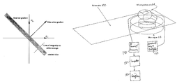
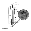
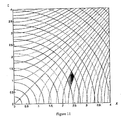
• FIG. 1 illustrates an electromagnet constructed out of two concentric cylindrical segments where the inner cylinder subtends 270°, and the outer cylinder subtends 180°. As indicated, the FOV is a region of space exterior to the arcs of both cylinders.
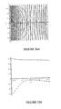
• FIG. 2 illustrates the properties of the magnetic field generated by the arrangement of conductors shown in FIG. 1, where the current on the inner cylinder is 0.6 units and the current on the outer cylinder is 2 units. FIG. 2(a) illustrates level contours of |B₀,| and field vectors (the essentially vertical lines), while FIG. 2(b) illustrates a plot of |B₀,| (solid line) and ∇|B₀|/|B₀|, (dashed line) along y=0.
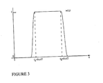
• FIG. 3 illustrates a graph of a typical normalized magnetization profile.
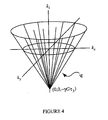
• FIG. 4 illustrates the cone that contains the samples points for F(ρ), showing some lines along which samples are acquired.
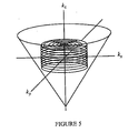
• FIG. 5 illustrates the cylinder within the cone, in which the sample points for the regridded data lie.
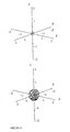
• FIGS. 6(a) and 6(b) respectively illustrate two level surfaces of B_0,εδ with b₀=1, ε=0.1, δ=0.0025.
• FIG. 7 illustrates slant slice imaging with an adjustable gradient of equal strength to the permanent gradient.
• FIG. 8 illustrates a timing diagram for the slant slice imaging method shown in FIG. 7.
• FIG. 9 illustrates an image created from measurements made with a permanent background field and the imaging sequence shown in FIG. 8.
• FIG. 10 illustrates slant slice imaging with an adjustable gradient of smaller strength than the permanent gradient.
• FIG. 11 illustrates level sets of G0+G1 (circular arcs) and G0-G1 (hyperbolas), where a slice is a region between two circular arcs and the slice averaging is along the hyperbolas.
• FIG. 12 shows images made using the slant-slice protocol with various values of the ratio $v=\frac{g_x}{g_z}.$
  The geometric distortion due to the slant of the read-out gradient is not corrected in these images.
• FIG. 13 shows images from FIG. 12 with the corrections for the geometric distortion.
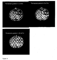
• FIG. 14 illustrates that when the ratio between G₀ and G₁ equals 1, their strengths are simultaneously increased.
• FIG. 15 illustrates a “one-sided” 3d MR-imaging system designed using the techniques of the invention wherein the sample (patient) would lie on a patient table to one side of the magnet.
DETAILED DESCRIPTION OF ILLUSTRATIVE EMBODIMENTS
• Certain specific details are set forth in the following description with respect to FIGS. 1-15 to provide a thorough understanding of various embodiments of the invention. Certain well-known details are not set forth in the following disclosure, however, to avoid unnecessarily obscuring the various embodiments of the invention. Those of ordinary skill in the relevant art will understand that they can practice other embodiments of the invention without one or more of the details described below. Also, while various methods are described with reference to steps and sequences in the following disclosure, the description is intended to provide a clear implementation of embodiments of the invention, and the steps and sequences of steps should not be taken as required to practice the invention.
• Overview
• The present invention relates to three problems that arise in magnetic resonance (MR) imaging: (1) excitation, (2) spatial encoding, and (3) image reconstruction. There are, of course, many other issues that would arise in the practical implementation of such an imaging system. Nonetheless these issues must be addressed first.
• First of all, one must understand what is meant by “imaging in an inhomogeneous background field” in accordance with the invention. At the outset, the problem of imaging with an inhomogeneous background field splits into two cases:
• [Noncritical case] The function |B₀| has no critical points in the field of view, the level sets of |B₀| are smooth, and fit together nicely.
• [Critical case] The function |B₀| has critical points within the field of view.
  The techniques available for spatial localization are different in each case and are treated separately.
• Because the local resonance frequency is determined by the magnitude of the local field, small variations in |B₀| are of much greater importance than small variations in its direction. In accordance with the invention, imaging is performed in an inhomogeneous background field if ∇|B₀| has a “large,” time independent component throughout the imaging experiment. The inventors are not considering the sorts of “random” or localized inhomogeneities that arise from the physical properties of the object being imaged, e.g. susceptibility artifacts. For much of this application, the inventors assume that the function |B₀| i “noncritical,” i.e., has no critical points in the field of view, the level sets of |B₀| are smooth, and fit together nicely. One can write:
  B ₀ =B ₀₀ +G ₀  (1)
  where B₀₀ is a constant uniform field, and the spatial variation of B₀ around the constant background is captured by G₀. The choice of B₀₀ is, a priori, rather arbitrary. One usually selects B₀₀ as the value of B₀ at a central point in the excited slice.
• The first problems that one encounters are connected to selective excitation. Because the permanent gradient tends to be large, a large RF-bandwidth may be required to excite a sufficiently wide slice. Beyond this bandwidth problem, one might also expect small variations in the direction of B₀ to lead to difficulties with selective excitation. However, this turns out to be a relatively minor problem. It can be shown mathematically that if the direction of B₀ does not vary too much, then a selective RF-pulse sequence excites spins lying in a region of space of the form:
  {(x,y,z): ω₀ −Δω≦γ|B ₀(x,y,z)|≦ω₀+Δω}  (2)
  If ∇|B₀| does not vanish within this set then the selected slice is a nonlinear analogue of the region between two planes.
• In the noncritical case, the permanent gradient in B₀ may be used as a slice select gradient. In this case, the problem of imaging in a noncritical, inhomogeneous field becomes, at least conceptually, the problem of imaging with a permanent slice select gradient. This is not an imposed gradient, which could be reversed, but rather a permanent and irreversible gradient that arises from the basic design of the imaging system and the placement of the sample. In the noncritical case, conditions on the background field may be obtained so that the measured signal can, up to appropriate changes in variable, be regarded as samples of a Fourier transform. In principle, the needed changes of variable can be computed with a knowledge of the background field, and the gradient fields throughout the field of view. The inventors' principal observation in this regard is that, so long as the direction of B₀ does not vary too much within the field of view, the most important property for the imaging system is to have a 2-parameter linear family of gradient fields. As explained below, the gradients themselves need not be linear.
• As a concrete example, consider the following situation: one has two infinite, concentric arcs of cylinders with current running in opposite directions, along their axes. The field of view is a region outside of both arcs. The setup is shown in FIG. 1. With infinitely long cylinders, the field is independent of the z-coordinate and lies in the xy-plane. FIG. 2(a) shows level lines of the field generated by the apparatus in FIG. 1, along with vectors indicating its local direction. FIG. 2(b) shows the field strength (solid line), and the relative gradient (dashed line) ∇|B₀|/|B₀|, along the y-axis.
• At each point (x,y,z), the direction of the background field, B₀(x,y,z), defines a “local z-direction.” The transverse component of the magnetization at (x,y,z) is the part of the magnetization orthogonal to B₀(x,y,z), This component of the magnetization precesses about B₀(x,y,z), at the local Larmor frequency, which equals γ|B₀(x,y,z)|. As the definition of the “rotating reference frame” varies from point to point, one may work in the laboratory reference frame.
• For purposes of the present patent application, the perturbations of B₀, used for spatial encoding (i.e. gradients), are referred to as “time independent” fields. Such fields are typically turned on for a period of time, and then turned off, and so are not, strictly speaking, time independent. With use this terminology to distinguish these fields from the RF-fields used for selective excitation. The RF-fields are constantly varying on the time scale of the Larmor period. The reason for this distinction is that, so long as B₀ is a very strong field, the important component of a “time independent” field is the component parallel to B₀ whereas the important components of an RF-field are those orthogonal to B₀. Throughout this description, it is assumed that the B₀-field is strong enough that the components of gradient fields, in directions orthogonal to it, can safely be ignored.
• B₀ is used to denote magnetic fields in the direction of B₀₀ In most applications of MR it is only the spatial dependence of the magnitude of B₀ which is carefully accounted for. Indeed it is usually assumed that the gradients are “linear” so that (in standard homogeneous field imaging):
  B₀₀=(0,0,b₀)  (3)
  B ₀ =B ₀₀+<(x,y,z),(g _x ,g _y ,g _z)>  (4)
  The linear function <(x,y,z),(g_x,g_y,g_z)> (or sometimes the vector (g_x,g_y,g_z) itself) is called the “gradient.” It is the projection of a gradient field in the direction of B₀. In the inhomogeneous case, one needs to be a bit more careful, and so the inventors work with the magnetic fields which generate the gradients. The present inventors distinguish between gradient fields, which are quasi-static magnetic fields used to induce perturbations in the background field and field gradients. Strictly speaking, the field gradient G generated by the gradient field G is defined to be: $\begin{array}{cc}G=\nabla \langle G,\frac{{\mathrm{<figure-callout\; id="0"\; label="B"\; filenames="US20060226837A1-20061012-D00002.png"\; state="\{\{state\}\}">B</figure-callout>}}_0}{{\mathrm{<figure-callout\; id="0"\; label="B"\; filenames="US20060226837A1-20061012-D00002.png"\; state="\{\{state\}\}">B</figure-callout>}}_0}\rangle & \left(5\right)\end{array}$
  If |G₀|<<|B₀| and G₀ is not too rapidly varying, then the following approximate value may be used: $\begin{array}{cc}G\approx \nabla \langle G,\frac{B_{00}}{B_{00}}\rangle ,& \left(6\right)\end{array}$
  for the field gradient, in the computations.
• In the MR-literature, a point where ∇|B₀| vanishes is sometimes called a “sweet spot.” Following the usual practice in the mathematics literature, such a point is called a critical point of |B₀|. The value of |B₀| at a critical point is called a critical value of |B₀|. The coordinates are normalized so that the critical point is located at (0,0,0) and if ω₀ denotes the critical value, then γ|B₀(0,0,0)|. The geometry of the level sets S_ω, for values of ω near to ω₀, is determined by the nature of the critical point that |B₀| has at (0,0,0). This is explained in Section 5 of [9]. Because the components of B₀ are harmonic functions, the function |B₀(x,y,z)| is subharmonic. The maximum principle implies that |B₀| cannot have a local maximum value. Thus (0,0,0) can be either a saddle point or a local minimum. To the inventors' knowledge, the only case that has been considered in the literature is that of a saddle point. This case is analyzed in detail in Section 6 of the aforementioned paper by Epstein, entitled, Magnetic Resonance Imaging in Inhomogeneous Fields, Inverse Problems, Vol. 20 (2004), pp. 753-780, where a new explanation is given as to why this is a problematic geometry for imaging. In this document, examples are constructed to show that magnetic fields exist such that |B₀| attains a nonzero local minimum value. These fields provide new opportunities for localized spectroscopy, which are not available in earlier approaches of this sort, e.g. FONAR and TOPICAL. In particular, with each acquisition, one can measure a complete FID generated by the material located in a single pixel.
• The measurement process for background fields without critical points within the field of view is considered below as well as how to construct fields so that |B₀| has an isolated minimum value.
• Inhomogeneous Fields without Critical Points
• Most approaches to magnetic resonance imaging in a homogeneous background field follow essentially the same sequence of steps:
• 1. The sample is polarized in the uniform background field.
• 2. Using a slice select gradient, the sample is selectively excited using an RF-pulse.
• 3. By reversing the slice select gradient, or using a refocusing pulse, the excited magnetization is rephased.
• 4. Using gradient fields, the excited magnetization is “spatially encoded.”
• 5. The signal is acquired, possibly with additional spatial encoding.
• In this first embodiment, the problem of imaging with an inhomogeneous background field without critical points is considered. A simplified model, with a background field, B₀(x,y,z), of the form:
  B ₀(x,y,z)=(b ₀ −Gz){circumflex over (z)}  (7)
  is considered for z∈[−z_max ,z _max]. While G/b₀ may be large, per unit distance, the field of view is constrained so that b₀±Gz_max is also assumed to be large. This means that B₀ is large within the field of view, and therefore, slowly varying perturbing fields, orthogonal to B₀, can safely be ignored. There are many possibilities for the placement of coils to generate the gradients and RF-pulses needed to do imaging. In some circumstances, these coils could be placed around the sample, in other cases they could be placed on one side of the sample. For a preliminary analysis, it is assumed that the gradient in |B₀| is parallel to the direction of B₀. This simplifies the discussion, a little, but is not necessary to do the analysis. A similar analysis also applies to fields which are not assumed to point in a fixed direction, provided |B₀| is large throughout the field of view, and ∇|B₀| does not vanish. This more general case is considered below.
• The following convention is used in this section: The Fourier transform of a function ƒ is denoted by F(ƒ). For the laboratory frame, {{circumflex over (x)},ŷ,{circumflex over (z)}}, with {circumflex over (z)} parallel to B₀., then:
  [a+ib,c]⇄a{circumflex over (x)}+bŷ+c{circumflex over (z)}  (8)
  with the complex number, a+ib, representing the transverse component of the magnetization. The computations in this section are done in the resonance rotating reference frame defined by b₀{circumflex over (z)}.
• In the analysis of fields without critical points, the permanent gradient in B₀. may be used as a slice select gradient. Leaving the sample stationary in the background field produces an equilibrium magnetization, M₀(x,y,z), given by:
  M ₀ =C(T)ρ′(x,y,z)B ₀(x,y,z)  (9)
  $\begin{array}{cc}C\left(T\right)=\frac{1.0075}{T}{\mathrm{Am}}^{-1}\mathrm{for}\mathrm{protons}\mathrm{in}\mathrm{water}.& \left(10\right)\end{array}$
  Here ρ′(x,y,z), is the density of water protons at (x,y,z). As noted, the constant C(T) is inversely proportional to T, the absolute temperature. To simplify notation, ρ denotes C(T)ρ′. A principal goal of MRI is the determination of the function ρ(x,y,z). If |B₀(x,y,z)| varies considerably over the support of ρ(x,y,z), then it may be necessary to include |B₀(x,y,z)| in the definition of the equilibrium magnetization. Such variation will result in a slowly varying shading of the image that can be removed by post-processing. In this section, it is assumed that this is not the case, and we use b₀ to denote |B₀(x,y,z)| in the formula for the equilibrium magnetization.
• In this embodiment, the slice select gradient does not have to be “turned on.” While the Bloch equation analysis of selective excitation applies, essentially verbatim, a few remarks are in order. If B₀ always points in the same direction, as in equation (7), then the usual analysis of selective excitation, from the homogeneous case, applies without change. In general, the direction of B₀. may vary slowly over the field of view. In this case, a selective RF-pulse designed for use with a B₀.-field having a permanent gradient, but uniform direction, may still be used as in equation (7). It may be shown mathematically that the main consequence of non-orthogonality between B₀. and B₁ is a decrease in the effective amplitude of B₁. If the angle between B₀(x,y,z) and B₁(x,y,z;t) is $\frac{\mathrm{<figure-callout\; id="2"\; label="\pi "\; filenames="US20060226837A1-20061012-D00003.png,US20060226837A1-20061012-D00006.png"\; state="\{\{state\}\}">\pi </figure-callout>}}{2}+\varphi ,$
  then the effective RF-field at this point is $\frac{\left(1+\cos \varphi \right)}{2}{\mathrm{<figure-callout\; id="1"\; label="B"\; filenames="US20060226837A1-20061012-D00006.png,US20060226837A1-20061012-D00009.png"\; state="\{\{state\}\}">B</figure-callout>}}_1\left(x,y,z;t\right).$
  Attenuating the RF slightly diminishes the flip angle and introduces a small phase error, but has very little effect on the selectivity of the pulse. If, over the extent of the sample, the angle between B₁ and B₀ is close to $\frac{\mathrm{<figure-callout\; id="2"\; label="\pi "\; filenames="US20060226837A1-20061012-D00003.png,US20060226837A1-20061012-D00006.png"\; state="\{\{state\}\}">\pi </figure-callout>}}{2},$
  then there will be some (removable) shading in the image. Hence, if B₁ is designed to excite spins with offset frequencies in the band about the Larmor frequency, [ƒ_min,ƒ_max], then the actual excited slice is given by the (possibly nonlinear) region of space
  {(x,y,z): ω₀+ƒ_min ≦γ|B ₀(x,y,z)|≦ω₀+ƒ_max}.
  The slices are bounded by level sets of |B₀(x,y,z)|.
• The first significant difference between imaging in homogeneous fields and in inhomogeneous fields occurs at step 3. In the latter case, it is not possible to reverse the slice select gradient to rephase the magnetization after the application of a selective pulse. The only realistic options are to use a self-refocused pulse or a refocusing pulse. A self refocused pulse, is only refocused once, so this option is not considered further.
• A normalized excitation profile is shown in FIG. 3. Assuming B₀ is given by equation (7), then, at the end of a selective RF-pulse, the magnetization is given by:
  M(x,y,z)=Cb ₀ρ(x,y,z)[e ^{iγGzτ 1} w(z),sgn(z)√{square root over (1−w ²(z))}]  (11)
  with τ₁ the rephasing time for the selective RF-pulse. The function sgn(z) takes the values ±1; it is included to allow for flip angles larger than 90°. In general sgn(z)=1 for z outside a finite band. If one were to immediately apply a refocusing pulse, then, at its conclusion, the magnetization would be given by:
  M(x,y,z)=Cb ₀ρ(x,y,z)[e ^−iγGzτ w(z),sgn(z)√{square root over (1−w ²(z))}]  (12)
  Normalizing so that t=0 at the conclusion of the refocusing pulse, the magnetization, as a function of space and time is given, for t≧0, by:
  M′(x,y,z;t)=Cb ₀ρ(x,y,z)[e ^{iγGz(t−τ 1 )} w(z),sgn(z)√{square root over (1−w ²(z))}]  (13)
  and therefore:
  M′(x,y,z,τ ₁)=Cb ₀ρ(x,y,z)[w(z),sgn(z)√{square root over (1−w ²(z))}]  (14)
  As has been known since the work of Hahn, one can create spin echoes, even with a permanent field gradient. The analysis is only slightly different if the direction of B₀ is slowly varying. This leads to small variations in the degree to which the magnetization is refocused which, in turn, produces a slowly varying shading in the reconstructed image.
• To measure the total density of spins within the slice, one could average the signal over a time interval [τ₁−τ_acq,τ₁+τ_acq] leading to a measured signal of the form: $\begin{array}{cc}{S}_{\mathrm{echo}}=C{\omega }_0^2{\int }_{o3}\mathrm{sinc}\left(\gamma \mathrm{Gz}{\tau }_{\mathrm{acq}}\right)b_{\mathrm{rec}1}\left(x,y,z\right)\rho \left(x,y,z\right)w\left(z\right)dxdydz.& \left(15\right)\end{array}$
  Here, it is assumed that τ_acq≦τ₁. Supposing that G is large, and Δz is the width of the excited slice, the requirement that sinc(γyGzτ_acq) remain positive throughout the excited slice leads to a maximum reasonable value for τ_acq: $\begin{array}{cc}{\tau }_{\mathrm{acq}}\le \frac{\pi }{\Delta f}\mathrm{where}\Delta f=\gamma G\mathrm{\Delta z}.& \left(16\right)\end{array}$
  Since the length of the time interval over which the signal is averaged effectively determines the bandwidth of the measured signal, it may be seen that, in inhomogeneous field imaging, the size of the permanent gradient effectively determines the minimum “receiver bandwidth.” This question is analyzed at length in Section 4 of the Epstein paper referenced above.
• In step 4, the encoding of spatial information, it is apparent from equation (13) that the phase of the transverse magnetization is marching inexorably forward. This suggests a stroboscopic approach to signal acquisition. By combining gradients with refocusing pulses, one could sample the Fourier transform of τ. How often this procedure can be repeated is largely determined by the size of T₂, and how well the magnetization can be repeatedly refocused. If the permanent gradient is large, then diffusion effects might also lead to a rapid decay of signal strength. This approach to the problem has been considered by several groups of investigators. For the most part, the previous work uses pulsed gradients for spatial encoding, and refocusing pulses to repeatedly refocus the accumulating phase in the direction of the permanent gradient. These ideas are described in U.S. Pat. No. 4,656,425, as well as in U.S. Pat. No. 5,023,554. The idea is further developed by Crowley and Rose as described in U.S. Pat. Nos. 5,493,225 and 5,304,930. Pulsed gradients are also used in SPRITE, though for different reasons.
• Crowley and Rose make the important observation that a large permanent gradient leads to a rapid traversal of k-space, and a short refocusing time. Accordingly, within the time constraints imposed by transverse relaxation, many samples can be collected. On the other hand, a large gradient means that, to excite a reasonably sized slice, requires a large RF-bandwidth and thereby an increased SAR. Indeed, as a refocusing pulse is required for each point sampled in k-space, these imaging sequences have a much larger SAR than most sequences used with homogeneous fields. In the afore-mentioned Epstein paper, the present inventor examined how SNR and SAR requirements limit the ratio |∇|B₀μ/|B₀|.
• Alternative approaches to the problem of spatial encoding and signal acquisition, which use a single refocusing pulse per line in k-space, will now be described. We first describe an embodiment using a 3-dimensional imaging protocol. Some applications of this idea lead to irregularly spaced samples, and so one might use a technique like regridding to obtain regularly spaced samples, before reconstructing an image. An analogue of a phase encoding-frequency encoding method and a radial, pure frequency encoding method are described. The latter approach is described first.
• After the selective excitation, the magnetization is allowed to freely precess for an additional τ₂ units of time so that, after a refocusing pulse, the magnetization is given by:
  M(x,y,z)=Cb ₀ρ(x,y,z)[e ^{−iγGzτ 3} w(z),sgn(z)√{square root over (1−w ²(z))}]  (17)
  where τ₃=τ₁+τ₂. At this point, a gradient of the form:
  B _fe0=((g _x ,g _y,0),(x,y,z)){circumflex over (z)}  (18)
  is turned on. If t is normalized so that the end of the refocusing pulse occurs at t=0, then the transverse magnetization is given, for t≧0, by:
  M _xy(x,y,z;t)=Cb ₀ρ(x,y,z)e ^{iγ[Gz(t−τ 3 )+t(g x x+g y y)]} w(z)  (19)
  Sampling at times t∈{jΔt:j=0, . . . ,N}, one measures approximate values for {F({overscore (ρ)})(jΔk_x,jΔk_y,jΔk_z−k_zmax)}, where:
  {overscore (ρ)}(x,y,z)=Cb ₀ρ(x,y,z)b _1rec(x,y,z)w(z)  (20)
  and
  Δk _x =γg _x Δt,Δk _y =γg _y Δt,Δk _z =γGΔt  (21)
  By adjusting the coefficients of the gradient field, B_fe0, one can obtain samples of F(ρ) along straight lines lying within a cone, C, with vertex at (0,0,−γGτ₃), as shown in FIG. 4. By regridding, one can then obtain samples of F(ρ) which are uniformly spaced on a cylindrical grid, lying inside a cylinder, K contained within the cone C, as shown in FIG. 5. An image could then be reconstructed by using the standard Fourier transform in the z-direction and a filtered back-projection algorithm in the transverse plane.
• To use a method like regridding requires a certain amount of oversampling. For each sample point p_j on the regular grid within K, severally irregularly spaced samples must be collected in a neighborhood of p_j. It is also clear that samples from near the vertex of C may not be usable in the regridding process. Additionally, the samples become rather spread out as one crosses the k_z=0 plane. It may be preferable, to measure F(ρ)(k), for k with nonpositive k_z, and recover the values in the other half plane using the conjugate symmetry.
• It is clear that there are many possible variations on this general approach to spatial encoding. For example, one might begin with a larger τ₃ and a large initial gradient to first move the vertex of the cone to (k_x0,k_y0,k_z0). This constitutes a phase encoding step. After reducing the gradient, samples could then be collected along lines of the form: (k_x0,k_y0,k_z0)+tγ(g_x,g_y,G).
• Indeed, one could turn off the x and y gradients and collect samples of the Fourier transform of ρ along vertical lines in k-space. If the initial points (k_x0,k_y0,k_z0) are on a uniformly spaced grid in the (k_x,k_y)-plane, then a standard FFT could be used to reconstruct the image.
• 2-D Imaging Protocol
• A second embodiment using a 2-dimensional imaging protocol will now be described. In this case, the permanent gradient is employed, along with a field of the form G_ss=η₁ ^sG₁+η₂ ^sG₂, to define the slice selection direction, and a field transverse to this direction, G_re as the read out gradient. A third field of the form G_ph=λ(η₁ ^pG₁+η₂ ^pG₂) is used as a phase encoding gradient. To describe the invention, a simple case is first considered wherein all of the gradients are linearly varying magnetic fields. As usual, it is assumed that the background field B₀ is sufficiently strong throughout D that components of fields orthogonal to B₀ have a very small effect on the measurements and can safely be ignored.
• Analysis in the Linear Case
• Let us suppose that B₀₀=(0,0,b₀) and let:
  B ₀=(0,0,b ₀)+(*,*,g _z z)=B ₀₀ +G ₀
  G ₁=(*,*,x) and G ₂=(*,*,y)  (22)
  Here * is used to denote negligibly small field components orthogonal to (0,0,b₀). The permanent field gradient is of the form:
  G_z=(0,0,g_z)  (23)
  and we assume that one can generate fields η₁G₁+η₂G₂, with gradients of the form:
  G _η=η₁(1,0,0)+η₂(0,1,0)  (24)
  where |η_j|≦m_g.
  Strong Transverse Gradients (G₀≦G₁)
• The simplest case arises when m_gεg_z. In this case, one uses for the slice select gradient the field G_ss=g_zG₁+G₀, and for the read gradient, the field G_re=−g_zG₁+G₀. The phase encoding gradient field is then G_ph=λ(*,*,y), where λ assumes values in the range [−m_g,m_g]. The slice select field gradient is then G_ss=(g_z,0,g_z), while the read-out field gradient is G_re=(−g_z,0,g_z). With these fields, the approach to imaging in accordance with the invention is the following:
• • 1. Place the sample in the static field, B₀, long enough to polarize the nuclear spins.
  • 2. Turn on the gradient field g_zG₁ to attain a slice select field gradient G_ss=(g_z,0,g_z).
  • 3. Apply a selective RF-pulse to flip spins lying in the region of space where:
    ƒ₀ −Δƒ≦γ|B ₀ +g _z G ₁|≦ƒ₀+Δƒ,
    leaving the spins outside this region essentially in their equilibrium state. If ƒ₀=γb₀, then the region of space excited is the slanted slice given by:
    {(x,y,z): −Δƒ≦γg _z(x+z)≦Δƒ}  (25)
    If w(s) denotes a function that is 1 for −Δƒ≦s≦Δƒ and zero outside a slightly larger interval, and τ₀ denotes the rephasing time for the selective RF-pulse, at the conclusion of the RF-pulse the transverse magnetization has the form:
    m(x,y,z;0)=sin αρ(x,y,z)w(γg _z(x+z))e ^{iτ 0 γg 2 (x+z)}  (26)
    Here α is the flip angle and ρ is a spin density function, normalized to take account of the magnitude of the equilibrium magnetization, and τ₀ is the rephasing time for the RF-pulse.
  • 4. At the conclusion of the RF-pulse, the adjustable gradient g_zG₁ is switched off and the excited magnetization is allowed to precess under the influence of the permanent gradient G₀ for τ₁ units of time. At the end of the free precession period, a 180° refocusing pulse is applied, this produces a transverse magnetization of the form:
    m(x,y,z;1)=sin αρ(x,y,z)w(γg _z(x+z))e ^{−iγg z (τ 0 (x+z)+τ 1 z)}  (27)
  • 5. The magnetization is now rewound in preparation for read-out: the gradient field g_zG₁ is again turned on and the excited magnetization is allowed to freely precess in the field g_zG₁+G₀ for ${\mathrm{<figure-callout\; id="0"\; label="\tau "\; filenames="US20060226837A1-20061012-D00002.png"\; state="\{\{state\}\}">\tau </figure-callout>}}_0+\frac{1}{2}{\mathrm{<figure-callout\; id="1"\; label="\tau "\; filenames="US20060226837A1-20061012-D00006.png,US20060226837A1-20061012-D00009.png"\; state="\{\{state\}\}">\tau </figure-callout>}}_1$
    units of time. To phase encode, the gradient field is turned on: $G_{\mathrm{ph}}=\frac{-2{\mathrm{\lambda \tau }}_1}{2{\mathrm{<figure-callout\; id="0"\; label="\tau "\; filenames="US20060226837A1-20061012-D00002.png"\; state="\{\{state\}\}">\tau </figure-callout>}}_0+{\mathrm{<figure-callout\; id="1"\; label="\tau "\; filenames="US20060226837A1-20061012-D00006.png,US20060226837A1-20061012-D00009.png"\; state="\{\{state\}\}">\tau </figure-callout>}}_1}{g}_z{\mathrm{<figure-callout\; id="2"\; label="G"\; filenames="US20060226837A1-20061012-D00003.png,US20060226837A1-20061012-D00006.png"\; state="\{\{state\}\}">G</figure-callout>}}_2.$
    At the conclusion of this free precession period, the transverse magnetization takes the form: $\begin{array}{cc}m\left(x,y,z;2\right)=\sin \mathrm{\alpha \rho }\left(x,y,z\right)w\left(\gamma g_z\left(x+z\right)\right)e^{-i\frac{1}{2}\gamma g_z{\mathrm{<figure-callout\; id="1"\; label="\tau "\; filenames="US20060226837A1-20061012-D00006.png,US20060226837A1-20061012-D00009.png"\; state="\{\{state\}\}">\tau </figure-callout>}}_1\left(z-x+\lambda y\right)}& \left(28\right)\end{array}$
  • 6. To read out the magnetization, one immediately turns on the field −g_zG₁. If t=0 at the start of the acquisition, then the signal available for sampling is: $\begin{array}{cc}S\left(t\right)={\int }_D\sin \mathrm{\alpha \rho }\left(x,y,z\right)w\left(\gamma g_z\left(x+z\right)\right)e^{-i\frac{1}{2}\gamma g_t\left({\tau }_1-t\right)\left(z-x\right)}{e}^{-i\frac{1}{2}\gamma \lambda g_z{\mathrm{<figure-callout\; id="1"\; label="\tau "\; filenames="US20060226837A1-20061012-D00006.png,US20060226837A1-20061012-D00009.png"\; state="\{\{state\}\}">\tau </figure-callout>}}_{1}y}dxdydz& \left(29\right)\end{array}$
    One may change variables in this integral, letting a=z+x and b=z−x, to obtain: $\begin{array}{cc}S\left(t\right)=\frac{1}{2}{\int }_D\sin \alpha \rho \left(\frac{a-\mathrm{<figure-callout\; id="2"\; label="b"\; filenames="US20060226837A1-20061012-D00003.png,US20060226837A1-20061012-D00006.png"\; state="\{\{state\}\}">b</figure-callout>}}{2},y,\frac{a+b}{2}\right)w\left(\gamma g_{z}a\right)e^{-i\frac{1}{2}\gamma g_z\left({\tau }_1-t\right)b}{e}^{-i\frac{1}{2}\gamma \lambda g_z{\mathrm{<figure-callout\; id="1"\; label="\tau "\; filenames="US20060226837A1-20061012-D00006.png,US20060226837A1-20061012-D00009.png"\; state="\{\{state\}\}">\tau </figure-callout>}}_{1}y}dadydb& \left(30\right)\end{array}$
    This can be interpreted as the 2-dimensional Fourier transform of the slice average: $\begin{array}{cc}\stackrel{\_}{\rho }\left(y,b\right)=\frac{1}{2}{\int }_{\frac{f_0-\Delta f}{\gamma {\mathrm{<figure-callout\; id="0"\; label="g\; z\; f"\; filenames="US20060226837A1-20061012-D00002.png"\; state="\{\{state\}\}">g</figure-callout>}}_z}}^{\frac{f_{}}{}}\rho \left(\frac{a-\mathrm{<figure-callout\; id="2"\; label="b"\; filenames="US20060226837A1-20061012-D00003.png,US20060226837A1-20061012-D00006.png"\; state="\{\{state\}\}">b</figure-callout>}}{2},y,\frac{a+b}{2}\right)w\left(g_{z}a\right)da.& \left(31\right)\end{array}$
• The slice averaging is illustrated in FIG. 7. The signal is therefore: $\begin{array}{cc}S\left(t\right)=\int \stackrel{\_}{\rho }\left(y,b\right)e^{-i\frac{1}{2}\gamma g_z\left[\left({\tau }_1-t\right)b+\lambda {\tau }_{1}y\right]}dydb.& \left(32\right)\end{array}$
  At time t the signal is ρ(k(t)), where: $k\left(t\right)=\frac{\gamma {\mathrm{<figure-callout\; id="2"\; label="g\; z"\; filenames="US20060226837A1-20061012-D00003.png,US20060226837A1-20061012-D00006.png"\; state="\{\{state\}\}">g</figure-callout>}}_z}{2}\left(\lambda {\tau }_1,\left({\tau }_1-t\right)\right).$
  This pulse sequence is illustrated in the timing diagram shown in FIG. 8 and an image of a phantom using this approach is shown in FIG. 9.
• There are several possible variations in this approach that lead to the same result. For example, one could refocus immediately following the selective excitation. After the refocusing pulse, the magnetization would be allowed to freely precess, under the influence of the permanent gradient alone for 2τ₀ time units. At the conclusion of this free precession period, the magnetization could again be refocused. The signal would then be read out with read-out gradient equal to −g_zG₁, as before. At the start of the read out, the transverse magnetization would equal: $\begin{array}{cc}m\left(x,y,z;2^{\prime }\right)=\sin \alpha \rho \left(x,y,z\right)w\left(\gamma g_z\left(x+z\right)\right)e^{-i\frac{1}{2}\gamma g_z{\mathrm{<figure-callout\; id="0"\; label="\tau "\; filenames="US20060226837A1-20061012-D00002.png"\; state="\{\{state\}\}">\tau </figure-callout>}}_0\left(z-x+\lambda y\right)}& \left(33\right)\end{array}$
  Weak Transverse Gradients (G₀>>G₁)
• What makes the previous case especially simple is the assumption that the apparatus can produce adjustable gradients, with the strength of the field gradient at least equal to the strength of the permanent field gradient. This is by no means necessary for the method to succeed. The only modification is in the definition of the slice average {overscore (ρ)}(y,b). This more general case is now described.
• The following is an illustrative case, with many possible variations that will not be spelled out. Suppose that one can generate adjustable field gradients that are smaller than the magnitude of the permanent field gradient in B₀. As before it is assumed that:
  G₀=(*,*,g_zz),G₁=(*,*,x) and G₂=(*,*,y),
  and that one can generate ρ₁G₁+ρ₂G₂ where |η₁|,|η₂|<m_g<<g_z. The same steps are followed as described above. For the slice select gradient, one can use G₀+g_xG₁, as before one can use λg_xG₂ for phase encoding and G₀−g_xG₁ as the read out gradient. Supposing that a scheme is used with two refocusing pulses, the calculations above are not repeated but one skilled in the art will appreciate that the signal equation now reads: $\begin{array}{cc}S\left(t\right)={\int }_D\sin \alpha \rho \left(x,y,z\right)w\left(\gamma g_z\left(x+z\right)\right)e^{-i\frac{1}{2}\gamma g_z\left({\tau }_0-t\right)\left(g_{z}z-g_{x}x\right)}{e}^{-i\frac{1}{2}\gamma \lambda g_x{\mathrm{<figure-callout\; id="0"\; label="\tau "\; filenames="US20060226837A1-20061012-D00002.png"\; state="\{\{state\}\}">\tau </figure-callout>}}_{0}y}dxdydz& \left(34\right)\end{array}$
  This can also be interpreted as a 2d-Fourier transform of an average over the excited slice. The only difference between this case and the previous case is that the average is over lines that meet the slice at a fixed angle, not necessarily 90°. This is shown in FIG. 10.
• To see this analytically, the variables are changed setting: $\begin{array}{cc}a=\frac{g_{z}z-g_{x}x}{g}b=\frac{g_{z}x+g_{x}z}{g}& \left(35\right)\end{array}$
  where g=√{square root over (g_x ²+g_z ²)}. This gives: $\begin{array}{cc}\begin{array}{c}S\left(t\right)={\int }_D\sin \mathrm{\alpha \rho }\left(\frac{g_{z}b-g_{x}a}{g},y,\frac{g_{z}b-g_{x}b}{g}\right)\\ w\left(\frac{\gamma }{g}\left(\left(g_z^2-g_x^2\right)a+2g_z{g}_{x}b\right)\right)\\ e^{-i\frac{1}{2}\gamma g\left({\tau }_0-t\right)a}{e}^{-i\frac{1}{2}\gamma \lambda g_x{\mathrm{<figure-callout\; id="0"\; label="\tau "\; filenames="US20060226837A1-20061012-D00002.png"\; state="\{\{state\}\}">\tau </figure-callout>}}_{0}y}dbdyda\end{array}& \left(36\right)\end{array}$
  Changing variables in the b-integral, setting: $\begin{array}{cc}s=\frac{\left(g_z^2-g_x^2\right)a+2g_x{g}_z\mathrm{<figure-callout\; id="2"\; label="b\; g"\; filenames="US20060226837A1-20061012-D00003.png,US20060226837A1-20061012-D00006.png"\; state="\{\{state\}\}">b</figure-callout>}}{g^{}}b=\frac{\left(g_x^2-g_z^2\right)a+{\mathrm{<figure-callout\; id="2"\; label="g"\; filenames="US20060226837A1-20061012-D00003.png,US20060226837A1-20061012-D00006.png"\; state="\{\{state\}\}">g</figure-callout>}}^2\mathrm{<figure-callout\; id="2"\; label="s"\; filenames="US20060226837A1-20061012-D00003.png,US20060226837A1-20061012-D00006.png"\; state="\{\{state\}\}">s</figure-callout>}}{2g_x{g}_z}& \left(37\right)\end{array}$
  one obtains:
  S(t)=∫{overscore (ρ)}(a,y)e ^{−iγ(g(τ 0 −t)a+λτ 0 gy]} dyda  (38)
  where: $\begin{array}{cc}\stackrel{\_}{\rho }\left(a,y\right)=\frac{{\mathrm{<figure-callout\; id="2"\; label="g"\; filenames="US20060226837A1-20061012-D00003.png,US20060226837A1-20061012-D00006.png"\; state="\{\{state\}\}">g</figure-callout>}}^2}{2g_x{g}_z}\int \rho \left(\frac{\left(s-a\right)}{2g_x},y,\frac{g\left(s+a\right)}{2g_z}\right)w\left(g\gamma s\right)ds& \left(39\right)\end{array}$
  Thus, {overscore (ρ)} is ρ averaged along lines with slope (g_z,0,g_x). These are lines orthogonal to the read-out direction (−g_x,0,g_z), which are not, in general, parallel to the slice select direction (g_x,0,g_z). In the case at hand, the lines over which ρ is averaged make an angle θ with the slice select direction where: $\begin{array}{cc}\cos \theta =\frac{2g_x{g}_z}{g_x^2+{\mathrm{<figure-callout\; id="2"\; label="g\; z"\; filenames="US20060226837A1-20061012-D00003.png,US20060226837A1-20061012-D00006.png"\; state="\{\{state\}\}">g</figure-callout>}}_z^{}}.& \left(40\right)\end{array}$
  The length of the intersection of these lines with the selected slice is minimized when θ=90°, hence this length is slowly varying for θ close to 90°.
  The Dependence of SNR on the Permanent Gradient Strength
• The signal-to-noise ratio attainable using the procedures described above is now considered. The analysis of the SNR is essentially the same as it would be in a standard 2-dimensional imaging system. The main effects of a large permanent gradient are to reduce the physical thickness of the excited slice, thereby reducing the signal, as well as to reduce the allowable spacing, Δt, between the acquisition of successive samples, thereby increasing the receiver bandwidth. Suppose that one has a slice thickness d and a rectangular field-of-view of size L. If Δx denotes the (isotropic) pixel length, Δt is the acquisition time and N-samples are collected in each direction, then:
  SNR∝dΔx ² N√{square root over (Δt)}  (41)
• It is desired to understand how the strength of the permanent gradient and the ratio ν=g_x/g_z affects the SNR. This brings the FOV into the equation, along with the gradient strength. Suppose that: g=√{square root over (|G₀|²+|G₁|²)}, then, to avoid aliasing, one would need to take: $\begin{array}{cc}\Delta t\le \frac{\sqrt{1+{\mathrm{<figure-callout\; id="2"\; label="v"\; filenames="US20060226837A1-20061012-D00003.png,US20060226837A1-20061012-D00006.png"\; state="\{\{state\}\}">v</figure-callout>}}^2}}{\gamma g_{x}L}.& \left(42\right)\end{array}$
  Using that L=NΔx, combining (41) and (42) one obtains: $\begin{array}{cc}\mathrm{SNR}\propto d\Delta x\sqrt{\frac{L\left(1+v^2\right)}{g_x}}.& \left(43\right)\end{array}$
  Thus, the SNR is not directly affected by the presence of a strong permanent background gradient. It is indirectly affected, because in order to get the desired resolution the maximum frequency sampled in k-space must satisfy: $\begin{array}{cc}{k}_{\max }=\frac{1+{\mathrm{<figure-callout\; id="2"\; label="v"\; filenames="US20060226837A1-20061012-D00003.png,US20060226837A1-20061012-D00006.png"\; state="\{\{state\}\}">v</figure-callout>}}^2}{2d\left(1-v^2\right)}.& \end{array}$
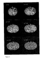
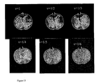
• If ν is close to zero (g_x=g_z), then a thin slice is needed to get high resolution. This has the effect of lowering the SNR and would necessitate using several averages of each line. Beyond this, a large gradient also may lead to a thin slice, if one is constrained in the amount of RF-power one may apply. This also diminishes the SNR. These effects are illustrated in FIGS. 12 and 13, which show images of a pomegranate obtained using different values for ν. FIG. 12 shows images of a pomegranate made using the slant-slice protocol with various values of the ratio $v=\frac{g_x}{g_z}.$
  In FIG. 12, the geometric distortion caused by the slant of the slice has not been corrected, whereas in FIG. 13 it has been. The applied (readout and slice select) gradients have amplitude 3 mT/m, and the amplitude of the permanent gradient ranged between 3 and 18 mT/m. The slice thickness in Hertz is kept fixed throughout these images, which in turn means that the slice thickness in mm decreases as the gradient strength increases. All images have the same intrinsic resolution. The SNR decrease is caused by the decrease in signal due to the thinning of the slice. The following parameters were used for the scan in FIG. 12: TE=12 ms, TR=400 ms, 256 PE steps, Scan time=102 sec., FOV=256×256 mm².
• FIG. 13 shows images from FIG. 12 with the corrections for the geometric distortion.
• On the other hand, as noted by Rose and Crowley, a strong permanent gradient causes k-space to be rapidly traversed and so one can, in principle, refocus the transverse magnetization and reread the same line several times. Indeed, the time to traverse a line in k-space is proportional to the strength of the read-out gradient. Hence, if ν is not too small, then within a single repeat time, one could refocus the magnetization and reread the line a number of times proportional to g, and thereby regain some of the lost SNR, without any increase in imaging time. In FIG. 14 we show images where the ratio between G₀ and G₁ equals 1, but their strengths are simultaneously increased. The slice thickness (in mm) is held constant. Notice the moderate decrease in the SNR as the gradient strength is increased. All images have the same intrinsic resolution.
• The Resolution in the Linear Case
• If one can generate an adjustable gradient of strength equal to that of the permanent gradient, then the pixels are rectangular and the resolution is determined by the usual heuristic formula: $\begin{array}{cc}\Delta x\approx \frac{1}{k_{\max }}.& \left(44\right)\end{array}$
  If the maximum adjustable gradient |G₁| is smaller than the permanent gradient, |G₀|, then there is additional averaging involved in signal acquisition. To quantify this effect one can make the following simplifying assumption: the spin density ρ is constant along lines parallel to the slice select direction. Indeed, this is also a “worst case” analysis, when comparing the slant slice protocol to a protocol with averaging parallel to the slice direction (i.e. |G₀|=|G₁|). This assumption is reasonable for thin slices and a slowly varying spin density. In this case, at least within the excited slice, one gets: $\begin{array}{cc}\rho \left(x,z\right)\approx f\left(\frac{-{\mathrm{xg}}_z+{\mathrm{zg}}_x}{g}\right).& \left(45\right)\end{array}$
  One uses g_x|G₁|,g_z=|G₀|, to simplify the notation. To simplify the analysis, one may ignore the third dimension, which would, in any case be obtained by phase encoding in a direction orthogonal to the plane spanned by G₀ and G₁.
• Ignoring the third dimension, the signal equation becomes: $\begin{array}{cc}S\left(t\right)={\int }_{-\frac{L}{2}}^{\frac{\mathrm{<figure-callout\; id="2"\; label="L"\; filenames="US20060226837A1-20061012-D00003.png,US20060226837A1-20061012-D00006.png"\; state="\{\{state\}\}">L</figure-callout>}}{2}}\left(\frac{{\mathrm{<figure-callout\; id="2"\; label="g"\; filenames="US20060226837A1-20061012-D00003.png,US20060226837A1-20061012-D00006.png"\; state="\{\{state\}\}">g</figure-callout>}}^2}{2g_x{g}_z}\right)\int f\left(a\frac{{\mathrm{<figure-callout\; id="2"\; label="g"\; filenames="US20060226837A1-20061012-D00003.png,US20060226837A1-20061012-D00006.png"\; state="\{\{state\}\}">g</figure-callout>}}^2}{2g_x{g}_z}-s\frac{g_z^2-{\mathrm{<figure-callout\; id="2"\; label="g\; x"\; filenames="US20060226837A1-20061012-D00003.png,US20060226837A1-20061012-D00006.png"\; state="\{\{state\}\}">g</figure-callout>}}_x^{}}{2g_x{g}_z}\right)w\left(g\gamma s\right)ds{e}^{-2\pi \mathrm{ika}}da,& \left(46\right)\end{array}$
  where 2πk=γ(τ₀−t)g. Letting: $\sigma =s\frac{g_z^2-{\mathrm{<figure-callout\; id="2"\; label="g\; x"\; filenames="US20060226837A1-20061012-D00003.png,US20060226837A1-20061012-D00006.png"\; state="\{\{state\}\}">g</figure-callout>}}_x^{}}{2g_x{g}_z}$
  obtains: $\begin{array}{cc}S\left(t\right)={\int }_{-\frac{L}{2}}^{\frac{\mathrm{<figure-callout\; id="2"\; label="L"\; filenames="US20060226837A1-20061012-D00003.png,US20060226837A1-20061012-D00006.png"\; state="\{\{state\}\}">L</figure-callout>}}{2}}\left(\frac{{\mathrm{<figure-callout\; id="2"\; label="g\; z"\; filenames="US20060226837A1-20061012-D00003.png,US20060226837A1-20061012-D00006.png"\; state="\{\{state\}\}">g</figure-callout>}}_z^{}+g_x^2}{g_z^2-g_x^2}\right)\int f\left(a\frac{{\mathrm{<figure-callout\; id="2"\; label="g"\; filenames="US20060226837A1-20061012-D00003.png,US20060226837A1-20061012-D00006.png"\; state="\{\{state\}\}">g</figure-callout>}}^2}{2g_x{g}_z}-\sigma \right)w\left(\gamma g\left(\frac{2\sigma g_x{g}_z}{g_z^2-g_x^2}\right)\right)d\sigma e^{-2\pi \mathrm{ika}}da,& \left(47\right)\end{array}$
  One final change of variables, gives this integral a very simple interpretation: $\begin{array}{cc}\alpha =a\frac{{\mathrm{<figure-callout\; id="2"\; label="g"\; filenames="US20060226837A1-20061012-D00003.png,US20060226837A1-20061012-D00006.png"\; state="\{\{state\}\}">g</figure-callout>}}^2}{2g_x{g}_z},& \left(48\right)\end{array}$
  obtains: $\begin{array}{cc}S\left(t\right)={\int }_{-\frac{L}{2}}^{\frac{\mathrm{<figure-callout\; id="2"\; label="L"\; filenames="US20060226837A1-20061012-D00003.png,US20060226837A1-20061012-D00006.png"\; state="\{\{state\}\}">L</figure-callout>}}{2}}\left(\frac{2g_x{g}_z}{g_z^2-g_x^2}\right)\int f\left(\alpha -\sigma \right)w\left(\gamma g\left(\frac{2\sigma g_x{g}_z}{g_z^2-g_x^2}\right)\right)d\sigma e^{-2\pi i\frac{g_x{\mathrm{<figure-callout\; id="2"\; label="g\; z\; g"\; filenames="US20060226837A1-20061012-D00003.png,US20060226837A1-20061012-D00006.png"\; state="\{\{state\}\}">g</figure-callout>}}_z}{g^{}}}d\alpha ,& \left(49\right)\end{array}$
• The measurement is the Fourier transform, at frequency $\frac{2g_x{\mathrm{<figure-callout\; id="2"\; label="g\; z\; g"\; filenames="US20060226837A1-20061012-D00003.png,US20060226837A1-20061012-D00006.png"\; state="\{\{state\}\}">g</figure-callout>}}_z}{g^{}}k,$
  of the convolution of ƒ with: $\begin{array}{cc}W\left(\sigma \right)=\left(\frac{2g_x{g}_z}{g_z^2-g_x^2}\right)w\left(\gamma g\frac{2\sigma g_x{g}_z}{g_z^2-g_x^2}\right).& \left(50a\right)\end{array}$
  Thus the slanted slice has three different effects on the resolution:
• • 1. It reduces the effective maximum frequency sampled by a factor of $\frac{2g_x{\mathrm{<figure-callout\; id="2"\; label="g\; z\; g"\; filenames="US20060226837A1-20061012-D00003.png,US20060226837A1-20061012-D00006.png"\; state="\{\{state\}\}">g</figure-callout>}}_z}{g^{}}$
    and scales the sample spacing in k-space by the same factor: $\begin{array}{cc}{k}_{\max ,\mathrm{ro}}=\frac{2g_x{\mathrm{<figure-callout\; id="2"\; label="g\; z\; g"\; filenames="US20060226837A1-20061012-D00003.png,US20060226837A1-20061012-D00006.png"\; state="\{\{state\}\}">g</figure-callout>}}_z}{g^{}}{k}_{\max }\mathrm{and}\Delta k_{\mathrm{ro}}=\frac{2g_x{\mathrm{<figure-callout\; id="2"\; label="g\; z\; g"\; filenames="US20060226837A1-20061012-D00003.png,US20060226837A1-20061012-D00006.png"\; state="\{\{state\}\}">g</figure-callout>}}_z}{g^{}}\Delta k& \left(50b\right)\end{array}$
  • 2. It causes blurring due to the convolution with W along the slanted line. As g_x approaches g_z the convolution approaches convolution with a scaled delta function.
  • 3. If the angle θ is close to zero, so that the effect of the convolution with W cannot be removed, then the effective field of view is the support of W*ƒ, rather than the support of ƒ.
    The effect of the convolution can, in principle, be removed if the Fourier transform of W does not vanish in the interval $\left[-\frac{2\mathrm{<figure-callout\; id="1"\; label="v"\; filenames="US20060226837A1-20061012-D00006.png,US20060226837A1-20061012-D00009.png"\; state="\{\{state\}\}">v</figure-callout>}}{1+{\mathrm{<figure-callout\; id="2"\; label="v"\; filenames="US20060226837A1-20061012-D00003.png,US20060226837A1-20061012-D00006.png"\; state="\{\{state\}\}">v</figure-callout>}}^2}{k}_{\max },\frac{2\mathrm{<figure-callout\; id="1"\; label="v"\; filenames="US20060226837A1-20061012-D00006.png,US20060226837A1-20061012-D00009.png"\; state="\{\{state\}\}">v</figure-callout>}}{1+{\mathrm{<figure-callout\; id="2"\; label="v"\; filenames="US20060226837A1-20061012-D00003.png,US20060226837A1-20061012-D00006.png"\; state="\{\{state\}\}">v</figure-callout>}}^2}{k}_{\max }\right].$
    Suppose that w(s)=χ_[−γd,γd](s), then $\begin{array}{cc}\hat{W}\left(k\right)=\frac{2v}{\pi \left(1-v^2\right)k}\sin \left(\pi \mathrm{dk}\frac{1-{\mathrm{<figure-callout\; id="2"\; label="v"\; filenames="US20060226837A1-20061012-D00003.png,US20060226837A1-20061012-D00006.png"\; state="\{\{state\}\}">v</figure-callout>}}^2}{2v}\right).& \left(50c\right)\end{array}$
    Hence, the effect of the slant slice convolution can be removed, without excessive amplification of the noise, for frequencies that satisfy: $\begin{array}{cc}k<<\frac{v}{d\left(1-v^2\right)}.& \left(51\right)\end{array}$
    Recalling that k_max is also scaled, the resolution is effectively given by $\begin{array}{cc}\Delta x\approx \frac{1+{\mathrm{<figure-callout\; id="2"\; label="v"\; filenames="US20060226837A1-20061012-D00003.png,US20060226837A1-20061012-D00006.png"\; state="\{\{state\}\}">v</figure-callout>}}^2}{2v}\frac{1}{k_{\max }},& \left(52\right)\end{array}$
    provided: $\begin{array}{cc}{k}_{\max }<\frac{1}{2d}\frac{1+{\mathrm{<figure-callout\; id="2"\; label="v"\; filenames="US20060226837A1-20061012-D00003.png,US20060226837A1-20061012-D00006.png"\; state="\{\{state\}\}">v</figure-callout>}}^2}{1-{\mathrm{<figure-callout\; id="2"\; label="v"\; filenames="US20060226837A1-20061012-D00003.png,US20060226837A1-20061012-D00006.png"\; state="\{\{state\}\}">v</figure-callout>}}^2}.& \left(53\right)\end{array}$
    Note that k_max=γNΔtg if 2N+1 samples are collected. This shows that the resolution in the readout direction is effectively determined by g_x: $\Delta x\approx \frac{\sqrt{1+{\mathrm{<figure-callout\; id="2"\; label="v"\; filenames="US20060226837A1-20061012-D00003.png,US20060226837A1-20061012-D00006.png"\; state="\{\{state\}\}">v</figure-callout>}}^2}}{2\gamma N\Delta {\mathrm{tg}}_x}.$
    Putting together the two formula shows that this approach has an effective resolution limit: $\begin{array}{cc}\Delta x_{\lim }\approx d\frac{1-v^2}{v}=2d\frac{\sin \theta }{\cos \theta },& \left(54\right)\end{array}$
    where θ is the angle between the slice select direction and the direction along which the spin density is averaged. With this modality, it may be desirable to use thin slices, measured many times. In principle, this would allow the recovery of any lost resolution, though at the cost of additional acquisition time.
    Inhomogeneous Fields without Critical Points, General Case
• The general case of imaging with an inhomogeneous field without critical points is now considered. As before, the permanent gradient in the background field may be used as a slice select gradient, or part of a slice select gradient. Several investigators have obtained partial results in this direction. In the prior art, the analysis is either perturbative, or done with unnecessarily restrictive hypotheses on the background field or the gradients. In this embodiment, the inventors provide minimal hypotheses on the background and gradient fields under which the measurements can, after a change of variables in physical space, be interpreted as samples of the ordinary Fourier transform.
• The following notational conventions will be used: suppose that the object being imaged lies in a region of space that is denoted by D, where D is the field-of-view. The object is described by a density function ρ(x,y,z), supported in D. As usual B₀ denotes the background field.
• • 1. For purposes of the present description:
    φ₀(x,y,z)=|B₀(x,y,z)|,
    and suppose it takes values in [c₀,c₁], for points lying in D. The local Larmor frequency at (x,y,z) is γφ₀(x,y,z).
  • 2. If f is a real valued function defined in a region D, then for each c∈R:
    ƒ⁻¹(c)={(x,y,z)∈D:ƒ(x,y,z)=c}
    The initial assumptions concern the function φ₀(x,y,z):
  • (a) The function φ₀(x,y,z) has no critical points within the field-of-view. This means that the level sets:
    S _γc={(x,y,z)∈D:φ ₀(x,y,z)=c}  (55)
    are smooth. The level sets are labeled by the local Larmor frequency.
  • (b) It is assumed that the coordinates (x,y,z) are chosen so that each level set S_γc can be represented as a graph over a (fixed) region R in the (x,y)-plane. In other words, there is a smooth function z(x,y,c) so that φ₀(x,y,z(x,y,c))=c for c∈[c₀,c₁] and therefore:
    S _γc={(x,y,z(x,y,c)):(x,y)∈R}  (56)
    With these assumptions, the region D is the set:
    D={(x,y,z(x,y,c)):(x,y)∈R and ∈[c ₀ ,c ₁]}.
    The second assumption is not strictly necessary. Though, without something like it, one cannot expect to use the Fourier transform, in any simple way, to reconstruct the spin density. Indeed the mathematical analysis required becomes vastly more complicated.
• A formula will now be provided for the measured signal without additional gradients, which will later be modified to include the effect of gradients. Let ω₀ denote γφ₀(0,0,0), and assume that [ω₀−Δω,ω₀+Δω] is contained in [γc₀,γc₁]. Suppose that the polarized sample is irradiated with a selective RF-pulse designed to flip spins lying in the region where the local Larmor frequency lies between ω₀−Δω and ω₀+Δω. This can be described in terms of an excitation profile w(φ₀). For example, an ideal 90°-flip has excitation profile given by:
  w ₉₀(c)=1 for γc∈[ω ₀−Δω,ω₀+Δω]  (57)
  w ₉₀(c)=0 for γc∈[ω ₀−Δω,ω₀+Δω]  (58)
  After the initial RF-pulse, the signal as a function of time is given by: $\begin{array}{cc}\begin{array}{c}{\mathrm{<figure-callout\; id="0"\; label="S"\; filenames="US20060226837A1-20061012-D00002.png"\; state="\{\{state\}\}">S</figure-callout>}}_0\left(t\right)=C\gamma {\int }_D\rho \left(x,y,z\right){\mathrm{<figure-callout\; id="1"\; label="b"\; filenames="US20060226837A1-20061012-D00006.png,US20060226837A1-20061012-D00009.png"\; state="\{\{state\}\}">b</figure-callout>}}_{1\mathrm{rec}}\left(x,y,z\right){\mathrm{<figure-callout\; id="0"\; label="\phi "\; filenames="US20060226837A1-20061012-D00002.png"\; state="\{\{state\}\}">\varphi </figure-callout>}}_0^2\\ \left(x,y,z\right)w\left({\mathrm{<figure-callout\; id="0"\; label="\phi "\; filenames="US20060226837A1-20061012-D00002.png"\; state="\{\{state\}\}">\varphi </figure-callout>}}_0\left(x,y,z\right)\right)dxdydz\end{array}& \left(59\right)\end{array}$
  One factor of ω₀(x,y,z) comes from the definition of the equilibrium magnetization and the other comes from Faraday's Law. Time is labeled so that t=0 corresponds to the spin echo induced by a refocusing pulse as described in the previous section. Using the second assumption, the variables are changed to (x,y,c), obtaining: $\begin{array}{cc}{\mathrm{<figure-callout\; id="0"\; label="S"\; filenames="US20060226837A1-20061012-D00002.png"\; state="\{\{state\}\}">S</figure-callout>}}_0\left(t\right)=C\gamma {\int }_R{\int }_{c_0}^{{\mathrm{<figure-callout\; id="1"\; label="c"\; filenames="US20060226837A1-20061012-D00006.png,US20060226837A1-20061012-D00009.png"\; state="\{\{state\}\}">c</figure-callout>}}_1}\frac{\rho \left(x,y,c\right){\mathrm{<figure-callout\; id="1"\; label="b"\; filenames="US20060226837A1-20061012-D00006.png,US20060226837A1-20061012-D00009.png"\; state="\{\{state\}\}">b</figure-callout>}}_{1\mathrm{rec}}\left(x,y,c\right)}{{\partial }_z{\mathrm{<figure-callout\; id="0"\; label="\phi "\; filenames="US20060226837A1-20061012-D00002.png"\; state="\{\{state\}\}">\varphi </figure-callout>}}_0\left(x,y,z\left(x,y,c\right)\right)}{\mathrm{<figure-callout\; id="2"\; label="c"\; filenames="US20060226837A1-20061012-D00003.png,US20060226837A1-20061012-D00006.png"\; state="\{\{state\}\}">c</figure-callout>}}^{2}w\left(c\right)dcdxdy& \left(60\right)\end{array}$
  The denominator in equation (60) is computed using the chain rule. It is the Jacobian of the transformation (x,y,z)→φ₀(x,y,z). To simplify the notation ρ(x,y,c) and b_rec1(x,y,c) denote ρ(x,y,z(x,y,c)) and b_1rec(x,y,z(x,y,c)) respectively.
• As above, demodulating and averaging S₀(t) over a sufficiently small time interval [−τ_acq,τ_acq] gives: $\begin{array}{cc}\begin{array}{c}\stackrel{\_}{S}\left(0\right)=C\gamma {\int }_R{\int }_{c_0}^{{\mathrm{<figure-callout\; id="1"\; label="c"\; filenames="US20060226837A1-20061012-D00006.png,US20060226837A1-20061012-D00009.png"\; state="\{\{state\}\}">c</figure-callout>}}_1}\frac{\rho \left(x,y,c\right){\mathrm{<figure-callout\; id="1"\; label="b"\; filenames="US20060226837A1-20061012-D00006.png,US20060226837A1-20061012-D00009.png"\; state="\{\{state\}\}">b</figure-callout>}}_{1\mathrm{rec}}\left(x,y,c\right)}{{\partial }_z{\mathrm{<figure-callout\; id="0"\; label="\phi "\; filenames="US20060226837A1-20061012-D00002.png"\; state="\{\{state\}\}">\varphi </figure-callout>}}_0\left(x,y,z\left(x,y,c\right)\right)}\\ {\mathrm{<figure-callout\; id="2"\; label="c"\; filenames="US20060226837A1-20061012-D00003.png,US20060226837A1-20061012-D00006.png"\; state="\{\{state\}\}">c</figure-callout>}}^{2}w\left(c\right)\sin c\left({\tau }_{\mathrm{acq}}\left(\gamma c-{\omega }_0\right)\right)dcdxdy\end{array}& \left(61\right)\end{array}$
  If Δω is small enough, then: $\begin{array}{cc}\stackrel{\_}{S}\left(0\right)\approx C{\int }_R\frac{\rho \left(x,y,{\gamma }^{-1}{\omega }_0\right)b_{\mathrm{rec}1}\left(x,y,{\gamma }^{-1}{\omega }_0\right)}{{\partial }_z{\mathrm{<figure-callout\; id="0"\; label="\phi "\; filenames="US20060226837A1-20061012-D00002.png"\; state="\{\{state\}\}">\varphi </figure-callout>}}_0\left(x,y,z\left(x,y,{\gamma }^{-1}{\omega }_0\right)\right)}dxdy& \left(62\right)\end{array}$
  Up to a scale factor, this is the total spin density along the slice S_ω ⁰ , weighted by b_rec1/∂_zφ₀.
• The addition of gradients to resolve the 3-dimensional structure of ρ is now considered. As in the previous section, a scheme may be used that directly samples a 3-dimensional Fourier transform. Because the direction of B₀ varies, one needs to consider the properties of the actual gradient fields, and not simply their projections along a fixed direction. For this discussion, it is supposed that one can generate gradient fields in the region D, which can be represented as linear combinations of two basic gradient fields denoted by G₁ and G₂. They are solutions, defined in a neighborhood of D, of the time independent, vacuum Maxwell equation.
• As before, in order to do 3D-imaging in a straightforward manner we require two further assumptions about the gradient fields:
• • 3. For all pairs (η₁,η₂) satisfying |η_j≦η_max, j=1, 2, one can generate the field η₁G₁+η₂G₂.
  • 4. For each c∈[c₀,c₁], the map from R to a subset of the plane, defined by: $\begin{array}{cc}X=\frac{\langle {\mathrm{<figure-callout\; id="1"\; label="G"\; filenames="US20060226837A1-20061012-D00006.png,US20060226837A1-20061012-D00009.png"\; state="\{\{state\}\}">G</figure-callout>}}_1\left(x,y,z\right),{\mathrm{<figure-callout\; id="0"\; label="B"\; filenames="US20060226837A1-20061012-D00002.png"\; state="\{\{state\}\}">B</figure-callout>}}_0\left(x,y,z\right)\rangle }{{\mathrm{<figure-callout\; id="0"\; label="\phi "\; filenames="US20060226837A1-20061012-D00002.png"\; state="\{\{state\}\}">\varphi </figure-callout>}}_0\left(x,y,z\right)}& \left(63\right)\\ Y=\frac{\langle {\mathrm{<figure-callout\; id="2"\; label="G"\; filenames="US20060226837A1-20061012-D00003.png,US20060226837A1-20061012-D00006.png"\; state="\{\{state\}\}">G</figure-callout>}}_2\left(x,y,z\right),{\mathrm{<figure-callout\; id="0"\; label="B"\; filenames="US20060226837A1-20061012-D00002.png"\; state="\{\{state\}\}">B</figure-callout>}}_0\left(x,y,z\right)\rangle }{{\mathrm{<figure-callout\; id="0"\; label="\phi "\; filenames="US20060226837A1-20061012-D00002.png"\; state="\{\{state\}\}">\varphi </figure-callout>}}_0\left(x,y,z\right)}& \left(64\right)\end{array}$
    is one-to-one and has a smooth inverse.
• In standard imaging, with a background field given by B₀=(0,0,b₀), the basic gradient. fields are modeled as G₁=(z,0,x) and G₂=(0,z,y). It is well known that one can generate the linear combinations described in assumption 3 above. In this case X=x, Y=y, so both assumptions are easily seen to be satisfied.
• It will be appreciated by those skilled in the art that due to the linear nature of Maxwell's equations, if, using electromagnets, one can generate the fields G₁ and G₂, in the region D, then, by adjusting the currents, one can also generate the linear combinations called for in assumption 1. In and of itself, condition 3 is a consequence of Maxwell's equation. It is also the fundamental requirement for obtaining data that can be interpreted as samples of the Fourier transform of a function simply related to ρ.
• Assumption 4 is a bit harder to check in practice. If the direction of B₀ does not vary too much over the region D, then this condition is also easily satisfied. If {{tilde over (x)},{tilde over (y)},{tilde over (z)}} is an orthonormal frame such that B₀(0,0,0) is parallel to {tilde over (z)}, then it is easy to show that there are vacuum solutions of Maxwell's equations of the form:
  G ₁ =x{tilde over (z)}+a ₁ {tilde over (x)}+a ₂ {tilde over (y)} G ₂ =y{tilde over (z)}+a ₂ {tilde over (x)}+b ₂ {tilde over (y)}  (65)
  where a₁,a₂,b₁,b₂ are linear functions, vanishing at (0,0,0). With these solutions:
  X=x+h .o .t., Y=y+h .o .t.,
  here h .o .t . are terms vanishing quadratically at (0,0,0). Hence, if the field-of-view is not too large, or, alternately, the direction of B₀ does not vary too rapidly, then the pair (X,Y), defined by the fields given in equations (63) and (64), satisfies assumption 4.
• How the expression for the signal is modified by the addition of the gradient fields may now be seen. It is assumed that φ₀ is sufficiently large throughout the field of view so that one can ignore components of G₁ and G₂ orthogonal to B₀. Here a spatial encoding scheme is used like that described above. For each allowable pair (η₁, η₂) there is an expression for the signal: $\begin{array}{cc}{S}_{\left({\mathrm{<figure-callout\; id="1"\; label="\eta "\; filenames="US20060226837A1-20061012-D00006.png,US20060226837A1-20061012-D00009.png"\; state="\{\{state\}\}">\eta </figure-callout>}}_1,{\eta }_2\right)}\left(t\right)\approx \frac{C{\omega }_0^2}{\gamma }{\int }_{\circ 2}{\int }_{c_0}^{{\mathrm{<figure-callout\; id="1"\; label="c"\; filenames="US20060226837A1-20061012-D00006.png,US20060226837A1-20061012-D00009.png"\; state="\{\{state\}\}">c</figure-callout>}}_1}\frac{\rho \left(x,y,c\right){\mathrm{<figure-callout\; id="1"\; label="b"\; filenames="US20060226837A1-20061012-D00006.png,US20060226837A1-20061012-D00009.png"\; state="\{\{state\}\}">b</figure-callout>}}_{1\mathrm{rec}}\left(x,y,c\right)}{{\partial }_z{\mathrm{<figure-callout\; id="0"\; label="\phi "\; filenames="US20060226837A1-20061012-D00002.png"\; state="\{\{state\}\}">\varphi </figure-callout>}}_0\left(x,y,z\left(x,y,c\right)\right)}\mathrm{gw}\left(c\right)e^{\mathrm{i\gamma }\left[c\left(t-{\tau }_3\right)+t{\eta }_{1}X\left(x,y,c\right)+t{\eta }_{2}Y\left(x,y,c\right)\right]}dcdxdy.& \left(66\right)\end{array}$
  The time parameter is normalized so that the refocusing pulse ends at t=0, at which time, the gradient field η₁G₁+η₂G₂ is switched on.
• Using assumption 2, one can solve for x(X,Y,c) and y(X,Y,c) throughout the region of integration. Let J(X,Y,c) denote the Jacobian of this change of variables: dxdy=J(X,Y,c)dXdY. The expression for the signal becomes: $\begin{array}{cc}{S}_{\left({\mathrm{<figure-callout\; id="1"\; label="\eta "\; filenames="US20060226837A1-20061012-D00006.png,US20060226837A1-20061012-D00009.png"\; state="\{\{state\}\}">\eta </figure-callout>}}_1,{\eta }_2\right)}\left(t\right)\approx \frac{C{\omega }_0^2}{\gamma }{\int }_{c_0}^{{\mathrm{<figure-callout\; id="1"\; label="c"\; filenames="US20060226837A1-20061012-D00006.png,US20060226837A1-20061012-D00009.png"\; state="\{\{state\}\}">c</figure-callout>}}_1}{\int }_{\circ 2}\stackrel{\_}{\rho }\left(X,Y,c\right)w\left(c\right)e^{\mathrm{i\gamma }\left[c\left(t-{\tau }_3\right)+t{\eta }_{1}X+t{\eta }_{2}Y\right]}dXdYdc.& \left(67\right)\end{array}$
  where: $\begin{array}{cc}\stackrel{\_}{\rho }\left(X,Y,c\right)=\frac{\begin{array}{c}\rho \left(x\left(X,Y,c\right),y\left(X,Y,c\right),c\right)b_{1\mathrm{rec}}\\ \left(x\left(X,Y,c\right),y\left(X,Y,c\right),c\right)\end{array}}{{\partial }_z{\mathrm{<figure-callout\; id="0"\; label="\phi "\; filenames="US20060226837A1-20061012-D00002.png"\; state="\{\{state\}\}">\varphi </figure-callout>}}_0\left(x\left(X,Y,c\right),y\left(X,Y,c\right),c\right)}J\left(X,Y,c\right)& \left(68\right)\end{array}$
  Demodulating and sampling one can measure samples F(w{overscore (ρ)})(k_j), where, as before, the points {k_j} lie along straight lines within C. The normalization here is a little different from that used above. In the earlier case, with B₀ given by equation (7), is was not necessary to change variables in the “z-direction.”
• Up to a constant, the measured signal equals the ordinary Fourier transform of w{overscore (ρ)}(X,Y,c). Using a variety of reconstruction techniques, based on the Fourier transform, such as regridding and filtered back-projection, one can therefore reconstruct w{overscore (ρ)}(X,Y,c). To determine the original spin density requires a knowledge of b_1rec and the transformations:
  (x,y,z)⇄(x,y,c)⇄(X,Y,c)  (69)
  These in turn can be computed with a knowledge of the background field B₀ and the basic gradient fields G₁ and G₂. The necessary coordinate transformations are determined by the fields B₀, G₁ and G₂, which means that they can be computed once and stored. But for the need to do this reparameterization before displaying the image, the computational requirements for imaging with an inhomogeneous field are comparable to those found in X-ray CT. Using the phase encoding-frequency encoding approach described above, with uniform sample spacing, one could use a standard FFT for the reconstruction step.
• The conditions above on the background field and gradient fields are essentially that the functions: $\begin{array}{cc}{\mathrm{<figure-callout\; id="0"\; label="\phi "\; filenames="US20060226837A1-20061012-D00002.png"\; state="\{\{state\}\}">\varphi </figure-callout>}}_0\left(x,y,z\right),\frac{\langle {\mathrm{<figure-callout\; id="1"\; label="G"\; filenames="US20060226837A1-20061012-D00006.png,US20060226837A1-20061012-D00009.png"\; state="\{\{state\}\}">G</figure-callout>}}_1\left(x,y,z\right),{\mathrm{<figure-callout\; id="0"\; label="B"\; filenames="US20060226837A1-20061012-D00002.png"\; state="\{\{state\}\}">B</figure-callout>}}_0\left(x,y,z\right)\rangle }{{\mathrm{<figure-callout\; id="0"\; label="\phi "\; filenames="US20060226837A1-20061012-D00002.png"\; state="\{\{state\}\}">\varphi </figure-callout>}}_0\left(x,y,z\right)},\frac{\langle G_2\left(x,y,z\right),B_0\left(x,y,z\right)\rangle }{{\varphi }_0\left(x,y,z\right)}& \left(70\right)\end{array}$
  define a one-to-one map from the field-of-view to a set of the form [c₀,c₁]×R, with R a subset of i². Implicitly, it is assumed that the direction of B₀ does not vary too much within D. This assumption is needed in order to apply the analysis of selective excitation with an inhomogeneous background field presented in the afore-mentioned Epstein paper. In this case, one also expects the receive coil sensitivity, b_rec1, to be approximately constant (or a least bounded from below) within D. Under these conditions it may be seen that the size of the measured signal obtainable with an inhomogeneous field should be comparable to the signal that can be obtained with a homogeneous field. Because there is always a large gradient, diffusion effects may also diminish the signal.
  Analysis in the Non-Linear Case for the 2D Imaging Protocol
• This section briefly describes the needed modifications, for the 2D-slice embodiment, if the gradient fields G₀,G₁,G₂ are not linear but satisfy the conditions enumerated above. For simplicity, we first describe how this approach would be applied to image a 2-dimensional object, so that the slices are 1-dimensional. The modifications needed to image 3-dimensional object with 2-dimensional slices is described at the end of this section. A 2D protocol is described using two refocusing pulses. In this case, B₀=B₀₀+G₀, where B₀₀ is the uniform field B₀₀=(0,b₀). If G denotes an adjustable gradient field, then the local Larmor frequency is determined by: $\begin{array}{cc}{\mathrm{<figure-callout\; id="0"\; label="B"\; filenames="US20060226837A1-20061012-D00002.png"\; state="\{\{state\}\}">B</figure-callout>}}_0+G={\mathrm{<figure-callout\; id="0"\; label="b"\; filenames="US20060226837A1-20061012-D00002.png"\; state="\{\{state\}\}">b</figure-callout>}}_0+\langle \frac{2B_{00}+{\mathrm{<figure-callout\; id="0"\; label="G"\; filenames="US20060226837A1-20061012-D00002.png"\; state="\{\{state\}\}">G</figure-callout>}}_0+\mathrm{<figure-callout\; id="2"\; label="G"\; filenames="US20060226837A1-20061012-D00003.png,US20060226837A1-20061012-D00006.png"\; state="\{\{state\}\}">G</figure-callout>}}{2{\mathrm{<figure-callout\; id="0"\; label="b"\; filenames="US20060226837A1-20061012-D00002.png"\; state="\{\{state\}\}">b</figure-callout>}}_0},{\mathrm{<figure-callout\; id="0"\; label="G"\; filenames="US20060226837A1-20061012-D00002.png"\; state="\{\{state\}\}">G</figure-callout>}}_0+G\rangle +O\left(\frac{1}{b_0}\right)& \left(71\right)\end{array}$
  This equation shows that the validity of the assumption that, for the purposes of analyzing the MR-signal, the gradient fields can be replaced by their projections onto B₀, is equivalent to the assumption that:
  |G ₀ +G|<<b ₀  (72)
  This assumption pertains throughout the calculations that follow.
• Modifying the notation in the linear case, then: $\begin{array}{cc}{\mathrm{<figure-callout\; id="0"\; label="g"\; filenames="US20060226837A1-20061012-D00002.png"\; state="\{\{state\}\}">g</figure-callout>}}_0=\langle \frac{B_{00}}{{\mathrm{<figure-callout\; id="0"\; label="b"\; filenames="US20060226837A1-20061012-D00002.png"\; state="\{\{state\}\}">b</figure-callout>}}_0},{\mathrm{<figure-callout\; id="0"\; label="G"\; filenames="US20060226837A1-20061012-D00002.png"\; state="\{\{state\}\}">G</figure-callout>}}_0\rangle ,{\mathrm{<figure-callout\; id="1"\; label="g"\; filenames="US20060226837A1-20061012-D00006.png,US20060226837A1-20061012-D00009.png"\; state="\{\{state\}\}">g</figure-callout>}}_1=\langle \frac{B_{00}}{{\mathrm{<figure-callout\; id="0"\; label="b"\; filenames="US20060226837A1-20061012-D00002.png"\; state="\{\{state\}\}">b</figure-callout>}}_0},{\mathrm{<figure-callout\; id="1"\; label="G"\; filenames="US20060226837A1-20061012-D00006.png,US20060226837A1-20061012-D00009.png"\; state="\{\{state\}\}">G</figure-callout>}}_1\rangle .& \left(73\right)\end{array}$
  The assumptions on the fields G₀, G₁ imply that ∇g₀, ∇g₁ are linearly independent at every point within the field of view.
• As shown by Epstein in Magnetic Resonance Imaging in Inhomogeneous Fields, Inverse Problems, Vol. 20 (2004), pp. 753-780, provided the direction of B₀ does not vary too much within the field-of-view, the selective excitation step proceeds very much as in the linear case. After the sample becomes polarized in the background field B₀, one may turn on the field G₁ and expose the sample to a selective RF-pulse. If w(s) is the slice profile, then the magnetization at the conclusion of the α-RF-pulse is:
  m(0′)=sin αρ(x,z)w(γ(g ₀ +g ₁))e ^{iτ 0 γ(g 0 +g 1 )}  (74)
  The transverse component is non-zero in the non-linear region of space where:
  w(γ(g ₀(x,z)+g ₁(x,z)))≠0  (75)
  After a refocusing pulse:
  m(1′)=sin αρ(x,y)w(γ(g ₀ +g ₁))e ^{−iτ 0 γ(g 0} g ^{1 )}  (76)
  The field G₁ is turned off and the magnetization is allowed to freely precess for 2τ₀ time units and is once refocused giving:
  m(2′)=sin αρ(x,z)w(γ(g ₀ +g ₁))e ^{−iτ 0 γ(g 0 g 1 )}  (77)
• Finally, at t=0, the field −G₁ is again turned on to obtain the measured signal: $\begin{array}{cc}S\left(t\right)={\int }_D\sin \mathrm{\alpha \rho }\left(x,z\right)w\left(\gamma \left({\mathrm{<figure-callout\; id="0"\; label="g"\; filenames="US20060226837A1-20061012-D00002.png"\; state="\{\{state\}\}">g</figure-callout>}}_0+g_1\right)\right)e^{i\left(t-{\tau }_0\right)\gamma \left(g_0-g_1\right)}dxdz.& \left(78\right)\end{array}$
  Now using the basic assumptions, which imply that:
  gA=g ₀ +g ₁ gB=g ₀ −g ₁  (79)
  define coordinates throughout the region of space occupied by the object, D, and define a map onto a region D′ of R² topologically equivalent to a square. Let dxdz=g²J(A, B)dAdB, the coefficient j is used to normalize so that g²J≈1 near the “center” of the slice. The signal equation becomes: $\begin{array}{cc}\begin{array}{c}S\left(t\right)={\mathrm{<figure-callout\; id="2"\; label="g"\; filenames="US20060226837A1-20061012-D00003.png,US20060226837A1-20061012-D00006.png"\; state="\{\{state\}\}">g</figure-callout>}}^2{\int }_D\sin \mathrm{\alpha \rho }\left(x\left(A,B\right),z\left(A,B\right)\right)\\ w\left(\gamma \mathrm{gA}\right)e^{i\left(t-{\tau }_0\right)\gamma \mathrm{gB}}J\left(A,B\right)dAdB.\end{array}& \left(80\right)\end{array}$
  For each fixed B,A a (x(A, B), z(A, B)) traces a smooth curve in the xz-plane which is, in some sense, transverse to the slice. This is, of course, just the curve:
  g ⁻¹(g ₀(x,z)−g ₁(x,z))=B.
  Rewrite the signal as a 1-dimensional Fourier transform of the slice averaged function:
  {overscore (ρ)}(B)=g ²∫ρ(x(A,B),z(A,B))w(γgA)J(A,B)dA  (81)
  provides: $\begin{array}{cc}S\left(t\right)=\sin \alpha {\int }_D\stackrel{\_}{\rho }\left(B\right)e^{i\left(t-{\tau }_0\right)\gamma \mathrm{gB}}dB.& \left(82\right)\end{array}$
• The measurements are then samples of the Fourier transform of ρ. Samples of ρ can be reconstructed as a function of B. To reconstruct ρ in the slice defined −Δƒ≦g⁻¹γ(g₀+g₁)≦Δƒ, one only needs to invert the relations in equation (79) to solve for (xz) as functions of (A,B). Using the computation of J(A,B) one can also rescale the data according to the density of the individual slices. These steps are possible, at least numerically, if one knows the functions g₀(x,z),g₁(x,z).
• For concreteness the example is considered where g₀=z²,g₁=x². The functions A,B define coordinates in the half plane x>0: A=z²+x²,g₁=z²−x². The image of the positive quadrant is the region where A>|B|. The area forms are related by the equation: $\begin{array}{cc}\mathrm{dxdz}=\frac{\mathrm{<figure-callout\; id="2"\; label="dAdB"\; filenames="US20060226837A1-20061012-D00003.png,US20060226837A1-20061012-D00006.png"\; state="\{\{state\}\}">dAdB</figure-callout>}}{2\sqrt{A^2-{\mathrm{<figure-callout\; id="2"\; label="B"\; filenames="US20060226837A1-20061012-D00003.png,US20060226837A1-20061012-D00006.png"\; state="\{\{state\}\}">B</figure-callout>}}^2}}.& \left(83\right)\end{array}$
  FIG. 11 shows level lines of A and B in this quadrant. As illustrated, near to x=z the pixels are nearly rectilinear, but are less so near the axes. A typical pixel is shaded. The function ρ is given by: $\begin{array}{cc}\rho \left(B\right)={\int }_{-\Delta f}^{\Delta f}w\left(\gamma A\right)\rho \left(\sqrt{\frac{A-\mathrm{<figure-callout\; id="2"\; label="B"\; filenames="US20060226837A1-20061012-D00003.png,US20060226837A1-20061012-D00006.png"\; state="\{\{state\}\}">B</figure-callout>}}{2}},\sqrt{\frac{A+B}{2}}\right)\frac{\mathrm{dA}}{2\sqrt{A^2-{\mathrm{<figure-callout\; id="2"\; label="B"\; filenames="US20060226837A1-20061012-D00003.png,US20060226837A1-20061012-D00006.png"\; state="\{\{state\}\}">B</figure-callout>}}^2}}.& \left(84\right)\end{array}$
  From examination of FIG. 11, it is evident that the simple notions of pixel and resolution, which are used with linear gradients, are not especially meaningful in the strongly non-linear case. Indeed it is evident that resolution in the reconstructed image, when transformed back to physical coordinates, is unlikely to be either isotropic at most points in the image plane, or homogeneous across the image.
• Adding a third dimension is straightforward, given that one can generate two adjustable gradients G₁,G₂ so that the projections in the B₀-direction, g₀,g₁,g₂, define a smooth invertible mapping from the field of view to a region in R³ topologically equivalent to a cube. A field of the form G₀+g_sG₁ can be used for slice selection, multiples of G₂ can be used to phase encode, and G₀−g_sG₁ can be used as a read-out gradient. As explained in the afore-mentioned Epstein article, the measurements obtained in this way can be interpreted, after a change of physical (x-space) coordinates, as the Fourier transform of non-linear averages, of non-linear 2-dimensional slices of ρ(x,y,z).
• An advantage of the 2D approach of the invention is that it allows the usage of a magnet with a substantial permanent gradient to be used as the main magnet in an MR-imaging device. This is accomplished without significantly sacrificing either resolution, acquisition time or SNR. By using slanted slices one recovers, in almost its entirety, the formalism used to describe imaging with a homogeneous background field. In particular, one can use a simple FFT to reconstruct the image, along with a post-processing step to remove geometric distortions due to either non-linear gradient fields or to the slant slice acquisition. The method of the invention produces high quality images, with acquisition times comparable to what would be used in a standard imaging device.
• The inventors have quantified the inherent limitations of the method as regards SNR and resolution, and neither seems, in any way insuperable. As noted above, given a constant physical slice thickness, a large permanent gradient increases the noise in each acquired line in exactly inverse proportion to the time required to acquire the line. Hence, by refocusing and remeasuring these lines, one can recover all the lost SNR, without any increase in overall repeat time. If g_x<<g_z, then, for a given measurement time, this approach does have an intrinsically lower resolution than a standard imaging method, with a homogeneous background field. The only real constraint on the applicability of this method is that ν not be too small, which allows for an enormous increase in the latitude available to designers of practical, high resolution, time and SAR efficient MR-imaging systems.
• This technique could be used to build a “one-sided” 3d MR-imaging system as shown generally in FIG. 15, wherein the sample (patient) would lie on a patient table 100 to one side of the magnet 110. This could be used for open MR-systems, or specialized MR-systems, for example dental MR. In many of these applications, gradient and RF-coils 120 are situated near to or around the sample, which is itself placed to one side of the static field generating magnet 110. As illustrated in FIG. 15, the gradient coils are controlled by gradient amplifier and controller 130, while the RF coils are connected to RF transmitter/receiver 140, which provides output to computer 150 for processing of the image data for display on display device 160. In this configuration, one would not need to work against nature to design magnets with a very homogeneous field “outside the bore,” but can solve the easier problems associated with designing magnets that have fields with a moderate but smooth permanent gradient, which the approach of the invention uses to good advantage. One can even imagine how this technique could be applied to advantage in an application like well-logging. While direct inversion of the measurements leads to images with geometric distortion, this distortion is completely determined by the field gradients. For a given magnet and gradient set, the geometric transformations, needed to remove the distortion, could be computed once and stored.
• Fields with Local Minima
• If one could create a magnetic field, B₀ such that |B₀(x,y,z)| assumes an isolated nonzero minimum value, then one could measure localized spectroscopic data using a single RF-pulse. Suppose the minimum occurs at (x₀,y₀,z₀) and ω₀=γφ₀(x₀,y₀,z₀). A selective excitation which excites frequencies in the band [ω₀−Δω,ω₀+Δω] would only excite spins in the region of space bounded by the closed surface:
  S _{ω 0 +Δω}={(x,y,z):γφ₀(x,y,z)=ω₀+Δω}.
  The entire FID is then produced by spins lying in a bounded region of space, close to the critical point of φ₀. Examples of such fields will now be provided. These fields are obtained as perturbations of a uniform background field:
  B₀=[0,0,b₀].
• • For real parameters ε and δ:
    B _0,εδ =B ₀ +ε[x,−y,0]+δ[−2xz,0,(z ² −x ²)]  (85)
    It is an elementary computation to see that:
    ∇×B _0,εδ=0,∇×B _0εδ=0
    and therefore these vector fields define vacuum solutions of Maxwell's equations. The length of B_0,εδ may be computed as:
    |B _0,εδ ² =b ₀ ²+(ε²−2b ₀δ)x²+ε² y ²+2b ₀ δz ²−4εδx ² z+δ ²(x ² +z ²)²  (86)
    The function φ₀ equals the square root of |B_0,εδ|², and therefore: $\nabla {\mathrm{<figure-callout\; id="0"\; label="\phi "\; filenames="US20060226837A1-20061012-D00002.png"\; state="\{\{state\}\}">\varphi </figure-callout>}}_0=\frac{\nabla {{\mathrm{<figure-callout\; id="0"\; label="B"\; filenames="US20060226837A1-20061012-D00002.png"\; state="\{\{state\}\}">B</figure-callout>}}_{0,\mathrm{\varepsilon \delta }}}^2}{2{\mathrm{<figure-callout\; id="0"\; label="B"\; filenames="US20060226837A1-20061012-D00002.png"\; state="\{\{state\}\}">B</figure-callout>}}_{0,\mathrm{\varepsilon \delta }}}.$
    The critical points of φ₀, where φ₀ does not vanish, therefore agree with the critical points of |B_0,εδ|²|. At critical points, where φ₀≠0, the Hessian matrices satisfy: $\begin{array}{cc}{\mathrm{<figure-callout\; id="0"\; label="H\; \phi "\; filenames="US20060226837A1-20061012-D00002.png"\; state="\{\{state\}\}">H</figure-callout>}}_{{\varphi }_{}}=\frac{H_{{{\mathrm{<figure-callout\; id="0"\; label="B"\; filenames="US20060226837A1-20061012-D00002.png"\; state="\{\{state\}\}">B</figure-callout>}}_{0,\mathrm{\varepsilon \delta }}}^2}}{2{\mathrm{<figure-callout\; id="0"\; label="B"\; filenames="US20060226837A1-20061012-D00002.png"\; state="\{\{state\}\}">B</figure-callout>}}_{0,\mathrm{\varepsilon \delta }}}& \left(87\right)\end{array}$
    This shows that the types of the critical points agree as well.
• From equation (86), it is clear that φ₀ has critical point at (0,0,0). The Hessian is a diagonal matrix: $\begin{array}{cc}{\mathrm{<figure-callout\; id="0"\; label="H\; \phi "\; filenames="US20060226837A1-20061012-D00002.png"\; state="\{\{state\}\}">H</figure-callout>}}_{{\varphi }_{}}\left(0,0,0\right)=\frac{2}{{\mathrm{<figure-callout\; id="0"\; label="\phi "\; filenames="US20060226837A1-20061012-D00002.png"\; state="\{\{state\}\}">\varphi </figure-callout>}}_0\left(0,0,0\right)}\left(\begin{array}{ccc}{\varepsilon }^2-2{\mathrm{<figure-callout\; id="0"\; label="b"\; filenames="US20060226837A1-20061012-D00002.png"\; state="\{\{state\}\}">b</figure-callout>}}_0\mathrm{<figure-callout\; id="0"\; label="\delta "\; filenames="US20060226837A1-20061012-D00002.png"\; state="\{\{state\}\}">\delta </figure-callout>}& 0& 0\\ 0& {\mathrm{<figure-callout\; id="2"\; label="\varepsilon "\; filenames="US20060226837A1-20061012-D00003.png,US20060226837A1-20061012-D00006.png"\; state="\{\{state\}\}">\varepsilon </figure-callout>}}^2& 0\\ 0& 0& 2{\mathrm{<figure-callout\; id="0"\; label="b"\; filenames="US20060226837A1-20061012-D00002.png"\; state="\{\{state\}\}">b</figure-callout>}}_0\delta \end{array}\right)& \left(88\right)\end{array}$
  This demonstrates the following result:
• If δb₀>0 and ε²>2δb₀, then B_0,εδ is a vacuum solution of Maxwell's equations such that B_0,εδ has an isolated minimum at (0,0,0).
• The fields [x,−y,0] and [−2xz,0,z²−x²] are essentially standard gradient fields. Therefore B_0,εδ could be generated by using an arrangement of gradient coils within a standard homogeneous, high field magnet. FIG. 6 illustrates 2 level surfaces of B_0,εδ with b₀=1, ε=0.1, δ=0.0025.
SUMMARY
• It has been shown how a magnet producing an inhomogeneous field, without critical points, can be used to produce the background field for an MR-imaging system. In particular, the present invention illustrates that the main difficulty that one encounters with a inhomogeneous background field is that of refocusing the phase that accumulates along the direction of ∇|B₀|. Several methods for directly sampling the 3d-Fourier transform of ρ, or the 2d-Fourier transform of slices of ρ are outlined.
• Simple geometric criteria are provided for the MR measurements made, using an inhomogeneous background field and nonlinear gradients, to be samples of the Fourier transform, up to a single change of coordinates. This coordinate change is determined by the background field, B₀ and the basic gradient fields, G₁,G₂. As such it need only be computed once and stored. The computations strongly suggest that it should be possible to obtain a strong signal with a background field having substantial inhomogeneity.
• By analyzing well-known imaging methods which employ fields with sweet spots, it may be shown that the principle underlying this approach is nothing other than the classical principle of stationary phase. In the prior art, these sweets spots are of saddle type. The aforementioned paper of Epstein provides a simple geometric explanation for the difficulty of obtaining localized information with critical points of this type: When the signal is large, the excited volume of space is seen to be highly non-localized. Hence, it is only in the long time limit, when the signal has largely decayed, that spatially localized information is available. Examples of fields are constructed such that |B₀| has an isolated, nonzero local minimum. Using such a field one can obtain a well localized excitation, ab initio, thereby avoiding the most serious pitfall of earlier approaches to imaging with a sweet spot.
• In the paper of Epstein cited above, the inventor shows that an isolated non-zero, local minimum is not possible under various symmetry hypotheses. For translationally invariant fields, it may be seen that local minima can occur, which, due to the translational invariance, must occur along a line. It is shown in the Epstein paper that an axially symmetric field cannot have an isolated minimum. Again, because of the axial symmetry, such an isolated minimum would have to occur along the axis of symmetry.
• While the present invention has been described in connection with the preferred embodiments of the various figures, it is to be understood that other similar embodiments may be used or modifications and additions may be made to the described embodiment for performing the same function of the present invention without deviating therefrom. Those skilled in the art will appreciate that there may be limits on magnetic field inhomogeneity and the geometry of level sets near a critical point. There also may be limitations on RF-pulses in inhomogeneous fields as well as for critical points in fields with symmetry. Such limitations are described in the Epstein paper incorporated by reference above. Therefore, the present invention should not be limited to any single embodiment, but rather should be construed in breadth and scope in accordance with the appended claims.

Claims (17)

1. A method of imaging an object using an inhomogeneous magnetic resonance imaging apparatus, comprising:

placing the object to be imaged in an inhomogeneous background field B₀ for a sufficient time for the nuclear spins of a desired species to be polarized, the background field B₀ having no critical points within a field of view of the apparatus;

selectively exciting the polarized nuclear spins using standard selective excitation RF-pulse sequences from said apparatus so as to generate substantially homogeneous RF-fields within the field of view of the apparatus; and

spatially encoding phases of the excited nuclear spins using gradient fields G₁, G₂, wherein the functions |B₀|, <B₀, G₁>, <B₀, G₂> define coordinates within the field of view of the apparatus.

2. The method of claim 1, wherein a single refocusing pulse is used in said phase encoding step to provide phase and frequency encoding of the excited nuclear spins.

3. The method of claim 1, comprising the further step of performing image reconstruction by interpreting the spatially encoded excited nuclear spins as samples of the Fourier transform of a function of three physical variables and using Fourier inversion methods to recover images.

4. The method of claim 4, comprising the step of reconstructing a desired spin density function from |B₀|, <G₁,B₀>, <G₂,B₀> and the reconstructed image.

5. A method of imaging an object using an inhomogeneous magnetic resonance imaging apparatus, comprising:

placing the object to be imaged in an inhomogeneous background field B₀ for a sufficient time for the nuclear spins of a desired species to be polarized, the background field B₀ having a single critical point within a field of view of the apparatus such that |B₀| has an isolated non-zero local minimum; and

selectively exciting the polarized nuclear spins in a neighborhood of the non-zero local minimum using standard selective excitation RF-pulse sequences from said apparatus so as to generate substantially homogeneous RF-fields within the field of view of the apparatus.

6. An inhomogeneous magnetic resonance imaging device for imaging an object, comprising:

means for generating a magnetic resonance imaging sequence to image said object; and

means for generating a non-homogeneous background magnetic field B₀ having a permanent gradient that is used as a slice select gradient, wherein the non-homogeneous background magnetic field B₀ has no critical points within a field of view of the device and the background field B₀ has the following constraints:

the direction of the background field B₀ does not vary too much within the field of view of the device;

the strength of the background field B₀ remains sufficiently large throughout the field of view so that a local Larmor frequency may be determined to a high degree of accuracy by the components of at least one field parallel to B₀;

level sets of the functions |B₀| within the field of view are expressible as graphs of smooth functions over a region lying in a plane;

said means for generating said background field B₀ generates said background field B₀ and said means for generating said magnetic resonance imaging sequence to image said object generates fields G₁, G₂ such that the functions |B₀|, <B₀, G₁>, <B₀, G₂> define coordinates within the field of view of the device;

for parameters (η₁, η₂) lying in a predetermined range, said means for generating said background field B₀ and said means for generating said magnetic resonance imaging sequence to image said object generate the fields η₁G₁+η₂G₂.; and

said means for generating said background field B₀ and said means for generating said magnetic resonance imaging sequence to image said object generate substantially homogeneous RF-fields within the field of view of the device.

7. An inhomogeneous magnetic resonance imaging apparatus for imaging an object, comprising:

means for generating an inhomogeneous background field B₀ for a sufficient time for the nuclear spins of a desired species of the object to be polarized, the background field B₀ having a single critical point within a field of view of the apparatus such that |B₀| has an isolated non-zero local minimum;

means for selectively exciting the polarized nuclear spins in a neighborhood of the non-zero local minimum using standard selective excitation RF-pulse sequences so as to generate substantially homogeneous RF-fields within the field of view of the apparatus; and

means for generating a magnetic resonance imaging sequence to image said object.

8. A method of magnetic resonance imaging an object in the presence of a permanent background gradient, G₀, in the polarizing field, B₀, comprising:

selecting a 2-dimensional slice of the object for excitation that is not perpendicular to G₀;

exciting the selected 2-dimensional slice of the object by applying a selective RF-pulse in the presence of a slice selection gradient G_ss where G_ss is a linear combination of G₀ and a transverse gradient G_ss ^app, generated as a linear combination of basic gradient fields G₁, G₂ provided by a magnetic resonance scanner;

applying a readout gradient G_re where G_re is a linear combination of G₀ and a transverse gradient G_re ^app generated as a linear combination of G₁, G₂, where G_ss and G_re are not parallel at any point in the selected excited slice; and

reconstructing the selected excited slice of the object.

9. A method as in claim 8, further comprising phase encoding the selected excited slice with a gradient G_ph generated as a linear combination of G₁, G₂.

10. A method as in claim 8, wherein the functions X=(G₁, B₀), Y=(G₂, B₀) and Z |B₀(x,y,z)|, define local coordinates that map the field of view of the magnetic resonance scanner onto a region of space.

11. A method as in claim 10, wherein G_ss=B₀+G₁ and G_re=B₀−G₁.

12. A method as in claim 8, wherein the step of applying the readout gradient G_re further comprises applying at least one refocusing pulse.

13. A magnetic resonance imaging device that images an object in the presence of a permanent background gradient, G₀, in the polarizing field, B₀, comprising:

a magnetic resonance scanner that provides basic gradient fields G₁, G₂;

an RF generator and RF coils that excite a selected 2-dimensional slice of the object for excitation that is not perpendicular to G₀ by applying a selective RF-pulse in the presence of a slice selection gradient G_ss, where G_ss is a linear combination of G₀ and a transverse gradient G_ss ^app, generated as a linear combination of the basic gradient fields G₁, G₂ provided by the magnetic resonance scanner;

a gradient generator and gradient coils that apply a readout gradient G_re where G_re is a linear combination of G₀ and a transverse gradient G_re ^app generated as a linear combination of G₁, G₂, where G_ss and G_re are not parallel at any point in the selected excited slice; and

a processor that reconstructs the selected excited slice of the object.

14. A device as in claim 13, further comprising means for phase encoding the selected excited slice with a gradient G_ph generated as a linear combination of G₁, G₂.

15. A device as in claim 13, wherein the functions X=(G₁, B₀), Y=(G₂, B₀) and Z=∥B₀(x,y,z)∥, where G₀=ΔB₀, define local coordinates that map the field of view of the magnetic resonance scanner onto a region of space.

16. A device as in claim 15, wherein G_ss=B₀+G₁ and G_re=B₀−G₀.

17. A device as in claim 13, wherein the gradient generator applies the readout gradient G_re by applying at least one refocusing pulse.

Images