US10765373B2 - Real-time denoising and prediction for a continuous glucose monitoring system - Google Patents
Real-time denoising and prediction for a continuous glucose monitoring system Download PDFInfo
- Publication number
- US10765373B2 US10765373B2 US15/583,558 US201715583558A US10765373B2 US 10765373 B2 US10765373 B2 US 10765373B2 US 201715583558 A US201715583558 A US 201715583558A US 10765373 B2 US10765373 B2 US 10765373B2
- Authority
- US
- United States
- Prior art keywords
- time
- analyte
- transmitter
- sensor
- raw signals
- Prior art date
- Legal status (The legal status is an assumption and is not a legal conclusion. Google has not performed a legal analysis and makes no representation as to the accuracy of the status listed.)
- Active, expires
Links
- 238000012544 monitoring process Methods 0.000 title claims abstract description 124
- 239000008103 glucose Substances 0.000 title description 192
- WQZGKKKJIJFFOK-GASJEMHNSA-N Glucose Natural products OC[C@H]1OC(O)[C@H](O)[C@@H](O)[C@@H]1O WQZGKKKJIJFFOK-GASJEMHNSA-N 0.000 title description 190
- 239000012491 analyte Substances 0.000 claims abstract description 229
- 238000000034 method Methods 0.000 claims abstract description 90
- 238000001914 filtration Methods 0.000 claims abstract description 47
- 238000009499 grossing Methods 0.000 claims description 18
- 238000013528 artificial neural network Methods 0.000 claims description 4
- 238000005259 measurement Methods 0.000 description 52
- NOESYZHRGYRDHS-UHFFFAOYSA-N insulin Chemical compound N1C(=O)C(NC(=O)C(CCC(N)=O)NC(=O)C(CCC(O)=O)NC(=O)C(C(C)C)NC(=O)C(NC(=O)CN)C(C)CC)CSSCC(C(NC(CO)C(=O)NC(CC(C)C)C(=O)NC(CC=2C=CC(O)=CC=2)C(=O)NC(CCC(N)=O)C(=O)NC(CC(C)C)C(=O)NC(CCC(O)=O)C(=O)NC(CC(N)=O)C(=O)NC(CC=2C=CC(O)=CC=2)C(=O)NC(CSSCC(NC(=O)C(C(C)C)NC(=O)C(CC(C)C)NC(=O)C(CC=2C=CC(O)=CC=2)NC(=O)C(CC(C)C)NC(=O)C(C)NC(=O)C(CCC(O)=O)NC(=O)C(C(C)C)NC(=O)C(CC(C)C)NC(=O)C(CC=2NC=NC=2)NC(=O)C(CO)NC(=O)CNC2=O)C(=O)NCC(=O)NC(CCC(O)=O)C(=O)NC(CCCNC(N)=N)C(=O)NCC(=O)NC(CC=3C=CC=CC=3)C(=O)NC(CC=3C=CC=CC=3)C(=O)NC(CC=3C=CC(O)=CC=3)C(=O)NC(C(C)O)C(=O)N3C(CCC3)C(=O)NC(CCCCN)C(=O)NC(C)C(O)=O)C(=O)NC(CC(N)=O)C(O)=O)=O)NC(=O)C(C(C)CC)NC(=O)C(CO)NC(=O)C(C(C)O)NC(=O)C1CSSCC2NC(=O)C(CC(C)C)NC(=O)C(NC(=O)C(CCC(N)=O)NC(=O)C(CC(N)=O)NC(=O)C(NC(=O)C(N)CC=1C=CC=CC=1)C(C)C)CC1=CN=CN1 NOESYZHRGYRDHS-UHFFFAOYSA-N 0.000 description 51
- 238000004422 calculation algorithm Methods 0.000 description 39
- 239000000499 gel Substances 0.000 description 36
- 206010012601 diabetes mellitus Diseases 0.000 description 33
- 230000000670 limiting effect Effects 0.000 description 31
- 229940125396 insulin Drugs 0.000 description 27
- 210000004369 blood Anatomy 0.000 description 25
- 239000008280 blood Substances 0.000 description 25
- 102000004877 Insulin Human genes 0.000 description 24
- 108090001061 Insulin Proteins 0.000 description 24
- 238000004891 communication Methods 0.000 description 23
- 230000001939 inductive effect Effects 0.000 description 23
- 238000004458 analytical method Methods 0.000 description 21
- 230000008859 change Effects 0.000 description 17
- 239000013598 vector Substances 0.000 description 15
- 238000013459 approach Methods 0.000 description 14
- 230000008569 process Effects 0.000 description 14
- 239000000758 substrate Substances 0.000 description 13
- 230000006870 function Effects 0.000 description 12
- 238000005070 sampling Methods 0.000 description 12
- 239000000017 hydrogel Substances 0.000 description 11
- 230000002218 hypoglycaemic effect Effects 0.000 description 11
- 239000011159 matrix material Substances 0.000 description 11
- 208000001072 type 2 diabetes mellitus Diseases 0.000 description 11
- 230000003345 hyperglycaemic effect Effects 0.000 description 9
- CNQCVBJFEGMYDW-UHFFFAOYSA-N lawrencium atom Chemical compound [Lr] CNQCVBJFEGMYDW-UHFFFAOYSA-N 0.000 description 9
- 238000004519 manufacturing process Methods 0.000 description 9
- 230000005284 excitation Effects 0.000 description 8
- 201000001421 hyperglycemia Diseases 0.000 description 8
- 238000013488 ordinary least square regression Methods 0.000 description 8
- 238000003908 quality control method Methods 0.000 description 8
- 239000004065 semiconductor Substances 0.000 description 8
- 238000004364 calculation method Methods 0.000 description 7
- 238000011156 evaluation Methods 0.000 description 7
- 230000002641 glycemic effect Effects 0.000 description 7
- 230000001976 improved effect Effects 0.000 description 7
- 238000001727 in vivo Methods 0.000 description 7
- 210000001519 tissue Anatomy 0.000 description 7
- 238000007476 Maximum Likelihood Methods 0.000 description 6
- 210000000227 basophil cell of anterior lobe of hypophysis Anatomy 0.000 description 6
- 238000009739 binding Methods 0.000 description 6
- 230000001965 increasing effect Effects 0.000 description 6
- 238000003780 insertion Methods 0.000 description 6
- 230000037431 insertion Effects 0.000 description 6
- 230000003287 optical effect Effects 0.000 description 6
- 210000000496 pancreas Anatomy 0.000 description 6
- BASFCYQUMIYNBI-UHFFFAOYSA-N platinum Chemical compound [Pt] BASFCYQUMIYNBI-UHFFFAOYSA-N 0.000 description 6
- 238000007920 subcutaneous administration Methods 0.000 description 6
- 208000013016 Hypoglycemia Diseases 0.000 description 5
- 206010067584 Type 1 diabetes mellitus Diseases 0.000 description 5
- 239000002775 capsule Substances 0.000 description 5
- 230000015556 catabolic process Effects 0.000 description 5
- 238000006243 chemical reaction Methods 0.000 description 5
- 238000006731 degradation reaction Methods 0.000 description 5
- 238000009792 diffusion process Methods 0.000 description 5
- 238000012545 processing Methods 0.000 description 5
- 230000004044 response Effects 0.000 description 5
- 230000035945 sensitivity Effects 0.000 description 5
- 238000002560 therapeutic procedure Methods 0.000 description 5
- 206010022489 Insulin Resistance Diseases 0.000 description 4
- 239000000853 adhesive Substances 0.000 description 4
- 230000001070 adhesive effect Effects 0.000 description 4
- 230000008901 benefit Effects 0.000 description 4
- 238000004061 bleaching Methods 0.000 description 4
- 230000002354 daily effect Effects 0.000 description 4
- 230000006378 damage Effects 0.000 description 4
- 230000001934 delay Effects 0.000 description 4
- 238000001514 detection method Methods 0.000 description 4
- 201000010099 disease Diseases 0.000 description 4
- 208000037265 diseases, disorders, signs and symptoms Diseases 0.000 description 4
- 230000014509 gene expression Effects 0.000 description 4
- 238000002513 implantation Methods 0.000 description 4
- 210000004185 liver Anatomy 0.000 description 4
- 235000012054 meals Nutrition 0.000 description 4
- 230000003647 oxidation Effects 0.000 description 4
- 238000007254 oxidation reaction Methods 0.000 description 4
- 230000037081 physical activity Effects 0.000 description 4
- 229920000642 polymer Polymers 0.000 description 4
- 241000894007 species Species 0.000 description 4
- 102000004190 Enzymes Human genes 0.000 description 3
- 108090000790 Enzymes Proteins 0.000 description 3
- 102000005548 Hexokinase Human genes 0.000 description 3
- 108700040460 Hexokinases Proteins 0.000 description 3
- 230000006399 behavior Effects 0.000 description 3
- 230000007423 decrease Effects 0.000 description 3
- 230000007812 deficiency Effects 0.000 description 3
- 230000001419 dependent effect Effects 0.000 description 3
- 238000013461 design Methods 0.000 description 3
- 230000037213 diet Effects 0.000 description 3
- 235000005911 diet Nutrition 0.000 description 3
- 239000003269 fluorescent indicator Substances 0.000 description 3
- -1 for example Chemical compound 0.000 description 3
- 230000006872 improvement Effects 0.000 description 3
- 230000003914 insulin secretion Effects 0.000 description 3
- 238000011835 investigation Methods 0.000 description 3
- 238000011068 loading method Methods 0.000 description 3
- 230000007774 longterm Effects 0.000 description 3
- 210000000056 organ Anatomy 0.000 description 3
- 230000009467 reduction Effects 0.000 description 3
- 230000001105 regulatory effect Effects 0.000 description 3
- 230000027756 respiratory electron transport chain Effects 0.000 description 3
- 230000000007 visual effect Effects 0.000 description 3
- 208000017667 Chronic Disease Diseases 0.000 description 2
- 208000007342 Diabetic Nephropathies Diseases 0.000 description 2
- 208000032131 Diabetic Neuropathies Diseases 0.000 description 2
- 206010012689 Diabetic retinopathy Diseases 0.000 description 2
- 206010018473 Glycosuria Diseases 0.000 description 2
- MHAJPDPJQMAIIY-UHFFFAOYSA-N Hydrogen peroxide Chemical compound OO MHAJPDPJQMAIIY-UHFFFAOYSA-N 0.000 description 2
- 206010052341 Impaired insulin secretion Diseases 0.000 description 2
- NNJVILVZKWQKPM-UHFFFAOYSA-N Lidocaine Chemical compound CCN(CC)CC(=O)NC1=C(C)C=CC=C1C NNJVILVZKWQKPM-UHFFFAOYSA-N 0.000 description 2
- 230000009471 action Effects 0.000 description 2
- 210000000577 adipose tissue Anatomy 0.000 description 2
- MWPLVEDNUUSJAV-UHFFFAOYSA-N anthracene Chemical compound C1=CC=CC2=CC3=CC=CC=C3C=C21 MWPLVEDNUUSJAV-UHFFFAOYSA-N 0.000 description 2
- 230000001363 autoimmune Effects 0.000 description 2
- WQZGKKKJIJFFOK-VFUOTHLCSA-N beta-D-glucose Chemical compound OC[C@H]1O[C@@H](O)[C@H](O)[C@@H](O)[C@@H]1O WQZGKKKJIJFFOK-VFUOTHLCSA-N 0.000 description 2
- 210000004204 blood vessel Anatomy 0.000 description 2
- 125000005620 boronic acid group Chemical group 0.000 description 2
- 210000004027 cell Anatomy 0.000 description 2
- 239000011248 coating agent Substances 0.000 description 2
- 238000000576 coating method Methods 0.000 description 2
- 238000012937 correction Methods 0.000 description 2
- 230000034994 death Effects 0.000 description 2
- 231100000517 death Toxicity 0.000 description 2
- 230000003111 delayed effect Effects 0.000 description 2
- 208000033679 diabetic kidney disease Diseases 0.000 description 2
- 239000003814 drug Substances 0.000 description 2
- 230000000694 effects Effects 0.000 description 2
- 210000003722 extracellular fluid Anatomy 0.000 description 2
- 230000014101 glucose homeostasis Effects 0.000 description 2
- JYGXADMDTFJGBT-VWUMJDOOSA-N hydrocortisone Chemical compound O=C1CC[C@]2(C)[C@H]3[C@@H](O)C[C@](C)([C@@](CC4)(O)C(=O)CO)[C@@H]4[C@@H]3CCC2=C1 JYGXADMDTFJGBT-VWUMJDOOSA-N 0.000 description 2
- 230000010354 integration Effects 0.000 description 2
- 210000002414 leg Anatomy 0.000 description 2
- 229960004194 lidocaine Drugs 0.000 description 2
- 238000002690 local anesthesia Methods 0.000 description 2
- 238000007726 management method Methods 0.000 description 2
- 230000001404 mediated effect Effects 0.000 description 2
- 210000003205 muscle Anatomy 0.000 description 2
- 230000010355 oscillation Effects 0.000 description 2
- 230000002093 peripheral effect Effects 0.000 description 2
- 229910052697 platinum Inorganic materials 0.000 description 2
- 229920003229 poly(methyl methacrylate) Polymers 0.000 description 2
- 229920002338 polyhydroxyethylmethacrylate Polymers 0.000 description 2
- 239000004926 polymethyl methacrylate Substances 0.000 description 2
- 102000004169 proteins and genes Human genes 0.000 description 2
- 108090000623 proteins and genes Proteins 0.000 description 2
- 238000010791 quenching Methods 0.000 description 2
- 230000000171 quenching effect Effects 0.000 description 2
- 238000011160 research Methods 0.000 description 2
- 239000007787 solid Substances 0.000 description 2
- 238000003860 storage Methods 0.000 description 2
- 239000000126 substance Substances 0.000 description 2
- 208000024891 symptom Diseases 0.000 description 2
- 230000009897 systematic effect Effects 0.000 description 2
- 238000012360 testing method Methods 0.000 description 2
- 238000012549 training Methods 0.000 description 2
- 210000000707 wrist Anatomy 0.000 description 2
- UCTWMZQNUQWSLP-VIFPVBQESA-N (R)-adrenaline Chemical compound CNC[C@H](O)C1=CC=C(O)C(O)=C1 UCTWMZQNUQWSLP-VIFPVBQESA-N 0.000 description 1
- 229930182837 (R)-adrenaline Natural products 0.000 description 1
- 208000010444 Acidosis Diseases 0.000 description 1
- 206010000489 Acidosis hyperchloraemic Diseases 0.000 description 1
- 206010002383 Angina Pectoris Diseases 0.000 description 1
- 201000001320 Atherosclerosis Diseases 0.000 description 1
- 201000004569 Blindness Diseases 0.000 description 1
- ZOXJGFHDIHLPTG-UHFFFAOYSA-N Boron Chemical compound [B] ZOXJGFHDIHLPTG-UHFFFAOYSA-N 0.000 description 1
- 206010048962 Brain oedema Diseases 0.000 description 1
- 208000024172 Cardiovascular disease Diseases 0.000 description 1
- 208000001380 Diabetic Ketoacidosis Diseases 0.000 description 1
- 208000008960 Diabetic foot Diseases 0.000 description 1
- 208000005189 Embolism Diseases 0.000 description 1
- 208000001762 Gastric Dilatation Diseases 0.000 description 1
- 206010017865 Gastritis erosive Diseases 0.000 description 1
- 102000051325 Glucagon Human genes 0.000 description 1
- 108060003199 Glucagon Proteins 0.000 description 1
- 208000002705 Glucose Intolerance Diseases 0.000 description 1
- 206010018429 Glucose tolerance impaired Diseases 0.000 description 1
- 102000018997 Growth Hormone Human genes 0.000 description 1
- 108010051696 Growth Hormone Proteins 0.000 description 1
- 238000012404 In vitro experiment Methods 0.000 description 1
- 208000010415 Low Vision Diseases 0.000 description 1
- 239000004677 Nylon Substances 0.000 description 1
- 208000008589 Obesity Diseases 0.000 description 1
- 208000002193 Pain Diseases 0.000 description 1
- 208000018262 Peripheral vascular disease Diseases 0.000 description 1
- 208000004880 Polyuria Diseases 0.000 description 1
- 208000001435 Thromboembolism Diseases 0.000 description 1
- 206010052428 Wound Diseases 0.000 description 1
- 208000027418 Wounds and injury Diseases 0.000 description 1
- 210000001015 abdomen Anatomy 0.000 description 1
- 230000005856 abnormality Effects 0.000 description 1
- 238000002835 absorbance Methods 0.000 description 1
- 238000009825 accumulation Methods 0.000 description 1
- 239000002253 acid Substances 0.000 description 1
- 230000007950 acidosis Effects 0.000 description 1
- 208000026545 acidosis disease Diseases 0.000 description 1
- 239000000654 additive Substances 0.000 description 1
- 230000000996 additive effect Effects 0.000 description 1
- 150000001412 amines Chemical class 0.000 description 1
- 238000002266 amputation Methods 0.000 description 1
- 239000002260 anti-inflammatory agent Substances 0.000 description 1
- 229940124599 anti-inflammatory drug Drugs 0.000 description 1
- 239000003472 antidiabetic agent Substances 0.000 description 1
- 239000003963 antioxidant agent Substances 0.000 description 1
- 230000003078 antioxidant effect Effects 0.000 description 1
- 235000006708 antioxidants Nutrition 0.000 description 1
- 238000000149 argon plasma sintering Methods 0.000 description 1
- 210000001367 artery Anatomy 0.000 description 1
- QVGXLLKOCUKJST-UHFFFAOYSA-N atomic oxygen Chemical compound [O] QVGXLLKOCUKJST-UHFFFAOYSA-N 0.000 description 1
- 238000005311 autocorrelation function Methods 0.000 description 1
- 235000013405 beer Nutrition 0.000 description 1
- 230000002146 bilateral effect Effects 0.000 description 1
- 229920000249 biocompatible polymer Polymers 0.000 description 1
- 230000033228 biological regulation Effects 0.000 description 1
- 230000005540 biological transmission Effects 0.000 description 1
- 229910052796 boron Inorganic materials 0.000 description 1
- 208000006752 brain edema Diseases 0.000 description 1
- 230000001364 causal effect Effects 0.000 description 1
- 210000003169 central nervous system Anatomy 0.000 description 1
- 239000003153 chemical reaction reagent Substances 0.000 description 1
- 230000001684 chronic effect Effects 0.000 description 1
- 208000020832 chronic kidney disease Diseases 0.000 description 1
- 150000001875 compounds Chemical class 0.000 description 1
- 238000010276 construction Methods 0.000 description 1
- 238000005314 correlation function Methods 0.000 description 1
- 230000005574 cross-species transmission Effects 0.000 description 1
- 238000002790 cross-validation Methods 0.000 description 1
- 230000001186 cumulative effect Effects 0.000 description 1
- 238000007405 data analysis Methods 0.000 description 1
- 238000013480 data collection Methods 0.000 description 1
- 230000002950 deficient Effects 0.000 description 1
- 230000018044 dehydration Effects 0.000 description 1
- 238000006297 dehydration reaction Methods 0.000 description 1
- 230000006866 deterioration Effects 0.000 description 1
- 238000011161 development Methods 0.000 description 1
- 230000018109 developmental process Effects 0.000 description 1
- 238000000502 dialysis Methods 0.000 description 1
- 230000029087 digestion Effects 0.000 description 1
- 238000006073 displacement reaction Methods 0.000 description 1
- 238000010494 dissociation reaction Methods 0.000 description 1
- 230000005593 dissociations Effects 0.000 description 1
- 229940079593 drug Drugs 0.000 description 1
- 238000001647 drug administration Methods 0.000 description 1
- 230000005518 electrochemistry Effects 0.000 description 1
- 230000005520 electrodynamics Effects 0.000 description 1
- 238000001962 electrophoresis Methods 0.000 description 1
- 230000002255 enzymatic effect Effects 0.000 description 1
- 229960005139 epinephrine Drugs 0.000 description 1
- 230000003628 erosive effect Effects 0.000 description 1
- 210000003743 erythrocyte Anatomy 0.000 description 1
- 230000003203 everyday effect Effects 0.000 description 1
- 230000001747 exhibiting effect Effects 0.000 description 1
- 238000000605 extraction Methods 0.000 description 1
- 235000020937 fasting conditions Nutrition 0.000 description 1
- 235000013305 food Nutrition 0.000 description 1
- 210000001035 gastrointestinal tract Anatomy 0.000 description 1
- 230000002068 genetic effect Effects 0.000 description 1
- MASNOZXLGMXCHN-ZLPAWPGGSA-N glucagon Chemical compound C([C@@H](C(=O)N[C@H](C(=O)N[C@@H](CCC(N)=O)C(=O)N[C@@H](CC=1C2=CC=CC=C2NC=1)C(=O)N[C@@H](CC(C)C)C(=O)N[C@@H](CCSC)C(=O)N[C@@H](CC(N)=O)C(=O)N[C@@H]([C@@H](C)O)C(O)=O)C(C)C)NC(=O)[C@H](CC(O)=O)NC(=O)[C@H](CCC(N)=O)NC(=O)[C@H](C)NC(=O)[C@H](CCCNC(N)=N)NC(=O)[C@H](CCCNC(N)=N)NC(=O)[C@H](CO)NC(=O)[C@H](CC(O)=O)NC(=O)[C@H](CC(C)C)NC(=O)[C@H](CC=1C=CC(O)=CC=1)NC(=O)[C@H](CCCCN)NC(=O)[C@H](CO)NC(=O)[C@H](CC=1C=CC(O)=CC=1)NC(=O)[C@H](CC(O)=O)NC(=O)[C@H](CO)NC(=O)[C@@H](NC(=O)[C@H](CC=1C=CC=CC=1)NC(=O)[C@@H](NC(=O)CNC(=O)[C@H](CCC(N)=O)NC(=O)[C@H](CO)NC(=O)[C@@H](N)CC=1NC=NC=1)[C@@H](C)O)[C@@H](C)O)C1=CC=CC=C1 MASNOZXLGMXCHN-ZLPAWPGGSA-N 0.000 description 1
- 229960004666 glucagon Drugs 0.000 description 1
- 230000009229 glucose formation Effects 0.000 description 1
- 230000004153 glucose metabolism Effects 0.000 description 1
- 108010070004 glucose receptor Proteins 0.000 description 1
- 230000006377 glucose transport Effects 0.000 description 1
- 125000002791 glucosyl group Chemical group C1([C@H](O)[C@@H](O)[C@H](O)[C@H](O1)CO)* 0.000 description 1
- 108091005996 glycated proteins Proteins 0.000 description 1
- 239000000122 growth hormone Substances 0.000 description 1
- 229940088597 hormone Drugs 0.000 description 1
- 239000005556 hormone Substances 0.000 description 1
- 229960000890 hydrocortisone Drugs 0.000 description 1
- 229940126904 hypoglycaemic agent Drugs 0.000 description 1
- 210000003016 hypothalamus Anatomy 0.000 description 1
- 238000000338 in vitro Methods 0.000 description 1
- 208000015181 infectious disease Diseases 0.000 description 1
- 230000028709 inflammatory response Effects 0.000 description 1
- 238000001802 infusion Methods 0.000 description 1
- 230000002401 inhibitory effect Effects 0.000 description 1
- 238000002347 injection Methods 0.000 description 1
- 239000007924 injection Substances 0.000 description 1
- 238000001990 intravenous administration Methods 0.000 description 1
- 210000003734 kidney Anatomy 0.000 description 1
- 208000006443 lactic acidosis Diseases 0.000 description 1
- 150000002632 lipids Chemical class 0.000 description 1
- 239000004973 liquid crystal related substance Substances 0.000 description 1
- 230000007257 malfunction Effects 0.000 description 1
- 230000007246 mechanism Effects 0.000 description 1
- 239000012528 membrane Substances 0.000 description 1
- 230000002503 metabolic effect Effects 0.000 description 1
- 238000001690 micro-dialysis Methods 0.000 description 1
- 230000000116 mitigating effect Effects 0.000 description 1
- 239000000203 mixture Substances 0.000 description 1
- YHXISWVBGDMDLQ-UHFFFAOYSA-N moclobemide Chemical compound C1=CC(Cl)=CC=C1C(=O)NCCN1CCOCC1 YHXISWVBGDMDLQ-UHFFFAOYSA-N 0.000 description 1
- 238000012986 modification Methods 0.000 description 1
- 230000004048 modification Effects 0.000 description 1
- 238000012806 monitoring device Methods 0.000 description 1
- 208000010125 myocardial infarction Diseases 0.000 description 1
- 208000031225 myocardial ischemia Diseases 0.000 description 1
- 210000000653 nervous system Anatomy 0.000 description 1
- 230000002644 neurohormonal effect Effects 0.000 description 1
- 201000001119 neuropathy Diseases 0.000 description 1
- 230000007823 neuropathy Effects 0.000 description 1
- 231100000862 numbness Toxicity 0.000 description 1
- 229920001778 nylon Polymers 0.000 description 1
- 235000020824 obesity Nutrition 0.000 description 1
- 238000005457 optimization Methods 0.000 description 1
- 238000012261 overproduction Methods 0.000 description 1
- 230000001590 oxidative effect Effects 0.000 description 1
- 239000001301 oxygen Substances 0.000 description 1
- 229910052760 oxygen Inorganic materials 0.000 description 1
- 230000036407 pain Effects 0.000 description 1
- 230000036961 partial effect Effects 0.000 description 1
- 230000008506 pathogenesis Effects 0.000 description 1
- 230000001575 pathological effect Effects 0.000 description 1
- 230000007310 pathophysiology Effects 0.000 description 1
- 208000033808 peripheral neuropathy Diseases 0.000 description 1
- 238000011422 pharmacological therapy Methods 0.000 description 1
- 238000011458 pharmacological treatment Methods 0.000 description 1
- HXITXNWTGFUOAU-UHFFFAOYSA-N phenylboronic acid Chemical group OB(O)C1=CC=CC=C1 HXITXNWTGFUOAU-UHFFFAOYSA-N 0.000 description 1
- 230000035479 physiological effects, processes and functions Effects 0.000 description 1
- 206010036067 polydipsia Diseases 0.000 description 1
- 230000001737 promoting effect Effects 0.000 description 1
- 238000000746 purification Methods 0.000 description 1
- 238000011002 quantification Methods 0.000 description 1
- IUVKMZGDUIUOCP-BTNSXGMBSA-N quinbolone Chemical group O([C@H]1CC[C@H]2[C@H]3[C@@H]([C@]4(C=CC(=O)C=C4CC3)C)CC[C@@]21C)C1=CCCC1 IUVKMZGDUIUOCP-BTNSXGMBSA-N 0.000 description 1
- 238000005295 random walk Methods 0.000 description 1
- 239000003642 reactive oxygen metabolite Substances 0.000 description 1
- 238000011897 real-time detection Methods 0.000 description 1
- 230000002829 reductive effect Effects 0.000 description 1
- 238000007670 refining Methods 0.000 description 1
- 230000008060 renal absorption Effects 0.000 description 1
- 210000005084 renal tissue Anatomy 0.000 description 1
- 210000001525 retina Anatomy 0.000 description 1
- 238000012552 review Methods 0.000 description 1
- 230000037390 scarring Effects 0.000 description 1
- 230000003248 secreting effect Effects 0.000 description 1
- 230000028327 secretion Effects 0.000 description 1
- 230000035807 sensation Effects 0.000 description 1
- 238000004088 simulation Methods 0.000 description 1
- 230000037380 skin damage Effects 0.000 description 1
- 229910000679 solder Inorganic materials 0.000 description 1
- 239000000243 solution Substances 0.000 description 1
- 230000003595 spectral effect Effects 0.000 description 1
- 238000004611 spectroscopical analysis Methods 0.000 description 1
- 238000001228 spectrum Methods 0.000 description 1
- 238000004544 sputter deposition Methods 0.000 description 1
- 238000011272 standard treatment Methods 0.000 description 1
- 208000023516 stroke disease Diseases 0.000 description 1
- 208000011580 syndromic disease Diseases 0.000 description 1
- 150000003512 tertiary amines Chemical class 0.000 description 1
- 229940124597 therapeutic agent Drugs 0.000 description 1
- 230000032258 transport Effects 0.000 description 1
- 210000000689 upper leg Anatomy 0.000 description 1
- 210000002700 urine Anatomy 0.000 description 1
- 208000019553 vascular disease Diseases 0.000 description 1
- 230000007998 vessel formation Effects 0.000 description 1
- 239000013585 weight reducing agent Substances 0.000 description 1
- 230000029663 wound healing Effects 0.000 description 1
- 229910000859 α-Fe Inorganic materials 0.000 description 1
Images


Classifications
-
- A—HUMAN NECESSITIES
- A61—MEDICAL OR VETERINARY SCIENCE; HYGIENE
- A61B—DIAGNOSIS; SURGERY; IDENTIFICATION
- A61B5/00—Measuring for diagnostic purposes; Identification of persons
- A61B5/72—Signal processing specially adapted for physiological signals or for diagnostic purposes
- A61B5/7203—Signal processing specially adapted for physiological signals or for diagnostic purposes for noise prevention, reduction or removal
-
- A—HUMAN NECESSITIES
- A61—MEDICAL OR VETERINARY SCIENCE; HYGIENE
- A61B—DIAGNOSIS; SURGERY; IDENTIFICATION
- A61B5/00—Measuring for diagnostic purposes; Identification of persons
- A61B5/0002—Remote monitoring of patients using telemetry, e.g. transmission of vital signals via a communication network
- A61B5/0004—Remote monitoring of patients using telemetry, e.g. transmission of vital signals via a communication network characterised by the type of physiological signal transmitted
-
- A—HUMAN NECESSITIES
- A61—MEDICAL OR VETERINARY SCIENCE; HYGIENE
- A61B—DIAGNOSIS; SURGERY; IDENTIFICATION
- A61B5/00—Measuring for diagnostic purposes; Identification of persons
- A61B5/0002—Remote monitoring of patients using telemetry, e.g. transmission of vital signals via a communication network
- A61B5/0015—Remote monitoring of patients using telemetry, e.g. transmission of vital signals via a communication network characterised by features of the telemetry system
- A61B5/0024—Remote monitoring of patients using telemetry, e.g. transmission of vital signals via a communication network characterised by features of the telemetry system for multiple sensor units attached to the patient, e.g. using a body or personal area network
-
- A—HUMAN NECESSITIES
- A61—MEDICAL OR VETERINARY SCIENCE; HYGIENE
- A61B—DIAGNOSIS; SURGERY; IDENTIFICATION
- A61B5/00—Measuring for diagnostic purposes; Identification of persons
- A61B5/0002—Remote monitoring of patients using telemetry, e.g. transmission of vital signals via a communication network
- A61B5/0031—Implanted circuitry
-
- A—HUMAN NECESSITIES
- A61—MEDICAL OR VETERINARY SCIENCE; HYGIENE
- A61B—DIAGNOSIS; SURGERY; IDENTIFICATION
- A61B5/00—Measuring for diagnostic purposes; Identification of persons
- A61B5/0059—Measuring for diagnostic purposes; Identification of persons using light, e.g. diagnosis by transillumination, diascopy, fluorescence
- A61B5/0071—Measuring for diagnostic purposes; Identification of persons using light, e.g. diagnosis by transillumination, diascopy, fluorescence by measuring fluorescence emission
-
- A—HUMAN NECESSITIES
- A61—MEDICAL OR VETERINARY SCIENCE; HYGIENE
- A61B—DIAGNOSIS; SURGERY; IDENTIFICATION
- A61B5/00—Measuring for diagnostic purposes; Identification of persons
- A61B5/145—Measuring characteristics of blood in vivo, e.g. gas concentration, pH value; Measuring characteristics of body fluids or tissues, e.g. interstitial fluid, cerebral tissue
- A61B5/14503—Measuring characteristics of blood in vivo, e.g. gas concentration, pH value; Measuring characteristics of body fluids or tissues, e.g. interstitial fluid, cerebral tissue invasive, e.g. introduced into the body by a catheter or needle or using implanted sensors
-
- A—HUMAN NECESSITIES
- A61—MEDICAL OR VETERINARY SCIENCE; HYGIENE
- A61B—DIAGNOSIS; SURGERY; IDENTIFICATION
- A61B5/00—Measuring for diagnostic purposes; Identification of persons
- A61B5/145—Measuring characteristics of blood in vivo, e.g. gas concentration, pH value; Measuring characteristics of body fluids or tissues, e.g. interstitial fluid, cerebral tissue
- A61B5/14532—Measuring characteristics of blood in vivo, e.g. gas concentration, pH value; Measuring characteristics of body fluids or tissues, e.g. interstitial fluid, cerebral tissue for measuring glucose, e.g. by tissue impedance measurement
-
- A—HUMAN NECESSITIES
- A61—MEDICAL OR VETERINARY SCIENCE; HYGIENE
- A61B—DIAGNOSIS; SURGERY; IDENTIFICATION
- A61B5/00—Measuring for diagnostic purposes; Identification of persons
- A61B5/48—Other medical applications
- A61B5/4836—Diagnosis combined with treatment in closed-loop systems or methods
- A61B5/4839—Diagnosis combined with treatment in closed-loop systems or methods combined with drug delivery
-
- A—HUMAN NECESSITIES
- A61—MEDICAL OR VETERINARY SCIENCE; HYGIENE
- A61B—DIAGNOSIS; SURGERY; IDENTIFICATION
- A61B5/00—Measuring for diagnostic purposes; Identification of persons
- A61B5/72—Signal processing specially adapted for physiological signals or for diagnostic purposes
- A61B5/7235—Details of waveform analysis
- A61B5/7246—Details of waveform analysis using correlation, e.g. template matching or determination of similarity
-
- A—HUMAN NECESSITIES
- A61—MEDICAL OR VETERINARY SCIENCE; HYGIENE
- A61B—DIAGNOSIS; SURGERY; IDENTIFICATION
- A61B5/00—Measuring for diagnostic purposes; Identification of persons
- A61B5/72—Signal processing specially adapted for physiological signals or for diagnostic purposes
- A61B5/7235—Details of waveform analysis
- A61B5/725—Details of waveform analysis using specific filters therefor, e.g. Kalman or adaptive filters
-
- A—HUMAN NECESSITIES
- A61—MEDICAL OR VETERINARY SCIENCE; HYGIENE
- A61B—DIAGNOSIS; SURGERY; IDENTIFICATION
- A61B5/00—Measuring for diagnostic purposes; Identification of persons
- A61B5/72—Signal processing specially adapted for physiological signals or for diagnostic purposes
- A61B5/7235—Details of waveform analysis
- A61B5/7264—Classification of physiological signals or data, e.g. using neural networks, statistical classifiers, expert systems or fuzzy systems
-
- A—HUMAN NECESSITIES
- A61—MEDICAL OR VETERINARY SCIENCE; HYGIENE
- A61B—DIAGNOSIS; SURGERY; IDENTIFICATION
- A61B5/00—Measuring for diagnostic purposes; Identification of persons
- A61B5/72—Signal processing specially adapted for physiological signals or for diagnostic purposes
- A61B5/7271—Specific aspects of physiological measurement analysis
- A61B5/7275—Determining trends in physiological measurement data; Predicting development of a medical condition based on physiological measurements, e.g. determining a risk factor
-
- A—HUMAN NECESSITIES
- A61—MEDICAL OR VETERINARY SCIENCE; HYGIENE
- A61B—DIAGNOSIS; SURGERY; IDENTIFICATION
- A61B2560/00—Constructional details of operational features of apparatus; Accessories for medical measuring apparatus
- A61B2560/02—Operational features
- A61B2560/0204—Operational features of power management
- A61B2560/0214—Operational features of power management of power generation or supply
- A61B2560/0219—Operational features of power management of power generation or supply of externally powered implanted units
-
- A—HUMAN NECESSITIES
- A61—MEDICAL OR VETERINARY SCIENCE; HYGIENE
- A61B—DIAGNOSIS; SURGERY; IDENTIFICATION
- A61B2560/00—Constructional details of operational features of apparatus; Accessories for medical measuring apparatus
- A61B2560/02—Operational features
- A61B2560/0223—Operational features of calibration, e.g. protocols for calibrating sensors
-
- G—PHYSICS
- G16—INFORMATION AND COMMUNICATION TECHNOLOGY [ICT] SPECIALLY ADAPTED FOR SPECIFIC APPLICATION FIELDS
- G16H—HEALTHCARE INFORMATICS, i.e. INFORMATION AND COMMUNICATION TECHNOLOGY [ICT] SPECIALLY ADAPTED FOR THE HANDLING OR PROCESSING OF MEDICAL OR HEALTHCARE DATA
- G16H20/00—ICT specially adapted for therapies or health-improving plans, e.g. for handling prescriptions, for steering therapy or for monitoring patient compliance
- G16H20/10—ICT specially adapted for therapies or health-improving plans, e.g. for handling prescriptions, for steering therapy or for monitoring patient compliance relating to drugs or medications, e.g. for ensuring correct administration to patients
- G16H20/17—ICT specially adapted for therapies or health-improving plans, e.g. for handling prescriptions, for steering therapy or for monitoring patient compliance relating to drugs or medications, e.g. for ensuring correct administration to patients delivered via infusion or injection
Definitions
- the present invention relates generally to determining a concentration of analyte in a medium (e.g., interstitial fluid) of a living animal using a sensor implanted (partially or completely) in the living animal. Specifically, the present invention relates to real-time denoising a raw signal including an analyte-modulated component and converting the processed signal to an analyte concentration.
- a medium e.g., interstitial fluid
- Diabetes is a chronic disease that affects about 300 million people in the world. Diabetes therapy is mainly based on insulin, diet, drug administration, and physical exercise, tuned according to Self-Monitoring of Blood Glucose (SMBG) values collected three to four times a day.
- SMBG Blood Glucose
- the metabolic control based on SMBG is usually suboptimal, and glucose concentration often exceeds the normal range thresholds (70-180 mg/dl).
- CGM Continuous Glucose Monitoring
- CGM sensors are not approved to be used in place of SMBG for therapy adjustment and the suboptimal performance of CGM could negatively influence the correct functioning of applications based on it.
- three issues of relevance can be pointed out.
- hypoglycemic/hyperglycemic thresholds may help the mitigation of hypoglycemic/hyperglycemic critical events.
- the present invention overcomes the disadvantages of prior systems by (i) denoising raw signals using a real-time filtering technique and/or (ii) providing a more accurate and/or reliable predictions of analyte concentration. Further variations encompassed within the systems and methods are described in the detailed description of the invention below.
- an analyte monitoring system including an analyte sensor and a transmitter.
- the analyte sensor may include an indicator element that exhibits one or more detectable properties based on an amount or concentration of an analyte in proximity to the indicator element.
- the analyte sensor may be configured to generate one or more raw signals indicative of one or more analyte amounts or concentrations.
- the transmitter may be configured to (i) receive from the analyte sensor one or more raw signals indicative of analyte concentration and (ii) denoise the raw signal using a real-time filtering technique with one or more time-varying parameters.
- the real-time filtering technique includes Kalman filtering. In some embodiments, the real-time filtering technique compensates for the presence of one or more missing values in the received one or more raw signals.
- the real-time filtering technique may include estimating the one or more time-varying parameters.
- the one or more time-varying parameters may include an error variance ⁇ .
- the one or more time-varying parameters may include a parameter ⁇ 2 , where ⁇ represents a degree to which a slope from a current time window is desired to be close to the slope from a previous time window.
- the one or more time-varying parameters may be estimated occasionally.
- the one or more time-varying parameters may be estimated every 144 minutes using the last 6 hours of data.
- the one or more time-varying parameters may be estimated using a stochastically based smoothing criterion that is based on data of a burn-in interval.
- the transmitter may be further configured to predict ahead of time an analyte concentration based on one or more of the received one or more raw signals.
- an analyte monitoring system including an analyte sensor and a transmitter.
- the analyte sensor may include an indicator element that exhibits one or more detectable properties based on an amount or concentration of an analyte in proximity to the indicator element.
- the analyte sensor may be configured to generate one or more raw signals indicative of one or more analyte amounts or concentrations.
- the transmitter may be configured to (i) receive from the analyte sensor one or more raw signals indicative of analyte concentration and (ii) predict ahead of time an analyte concentration based on one or more of the received one or more raw signals using one or more prediction models.
- the transmitter may be configured to use a forgetting factor ⁇ to regulates how the received one or more raw signals are used to predict ahead of time the analyte concentration.
- the one or more prediction models may include a first-order polynomial model.
- the one or more prediction models may include a first-order autoregressive model.
- the one or more prediction models may include Kalman filtering.
- the one or more prediction models may include one or more artificial neural networks.
- the analyte monitoring method may include using an analyte sensor to generate one or more raw signals indicative of one or more analyte amounts or concentrations.
- the analyte sensor may include an indicator element that exhibits one or more detectable properties based on an amount or concentration of an analyte in proximity to the indicator element.
- the analyte monitoring method may include using a transmitter to receive from the analyte sensor one or more raw signals indicative of analyte concentration.
- the analyte monitoring method may include using the transmitter to denoise the raw signal using a real-time filtering technique with one or more time-varying parameters.
- the analyte monitoring method may include using an analyte sensor to generate one or more raw signals indicative of one or more analyte amounts or concentrations.
- the analyte sensor may include an indicator element that exhibits one or more detectable properties based on an amount or concentration of an analyte in proximity to the indicator element.
- the analyte monitoring method may include using a transmitter to receive from the analyte sensor one or more raw signals indicative of analyte concentration.
- the analyte monitoring method may include using the transmitter to predict ahead of time an analyte concentration based on one or more of the received one or more raw signals using one or more prediction models.
- FIG. 1 is a schematic view illustrating a glucose-insulin control system.
- FIG. 2 is a chart comparing between glycemic profiles obtained with self-monitoring of blood glucose (SMBG) system (filled circles) and continuous glucose monitoring (CGM) system (continuous line).
- SMBG blood glucose
- CGM continuous glucose monitoring
- FIG. 3 is a schematic view illustrating an analyte monitoring system embodying aspects of the present invention.
- FIG. 4 is a schematic view illustrating a sensor and transmitter of an analyte monitoring system embodying aspects of the present invention.
- FIG. 5 is cross-sectional, perspective view of a transmitter embodying aspects of the invention.
- FIG. 6 is an exploded, perspective view of a transmitter embodying aspects of the invention.
- FIG. 7 is a schematic view illustrating a transmitter embodying aspects of the present invention.
- FIG. 8A illustrates an analyte sensor (shown without an analyte-indicator hydrogel coating) embodying aspects of the present invention.
- FIG. 8B illustrates an analyte indicator of an analyte sensor embodying aspects of the present invention.
- FIG. 8C illustrates the chemical structure and glucose binding mode of indicator moiety of a sensor embodying aspects of the present invention.
- FIG. 9 illustrates one or more functions that may be performed by an analyte monitoring system embodying aspects of the present invention.
- FIG. 10 illustrates indicator normalized modulation VS glucose concentration embodying aspects of the present invention.
- FIG. 11 illustrates the reactions and kinetics of the related species of the indicator molecules of a sensor embodying aspects of the present invention.
- FIG. 12 illustrates the components of the excitation light received by the photodetector that contribute to the offset in the raw signal in an analyte monitoring system embodying aspects of the present invention.
- FIG. 13 illustrates the theoretical relationship between interstitial and plasma glucose according to some embodiments of the present invention.
- FIGS. 14-17 illustrate CGM data, YSI values, and the Finger Stick (FS) measurements of a representative sensor embodying aspects of the present invention during different time periods.
- FIG. 18 is a table illustrating ROC accuracy with respect to the concurrence of CGM and hexokinase trends embodying aspects of the present invention.
- FIG. 19 illustrates a representative sensor in Dataset 2 .
- the CGM data is shown with a solid line, the YSI values are shown with circles, and the Finger Sticks (FS) measurements are shown with +s.
- FS Finger Sticks
- FIGS. 20A, 20B, and 20C are graphs showing estimated error variance day-by-day (thin line with circles) with sensor's mean (thin line) and global mean error variance (thick line) for three different sensors.
- FIGS. 21A-21D are graphs illustrating CGM data (thick line) versus smoothed signal (thin line) during a first time window, weighted residuals (circles) during the first time window, CGM data (thick line) versus smoothed signal (thin line) during a second time window, and weighted residuals (circles) during the second time window, respectively, for a representative sensor.
- FIGS. 22A-22C are graphs illustrating CGM data (thin line) versus KF series (thick line) for a representative sensor during first, second, and third time periods, respectively.
- FIGS. 23A-23C are graphs illustrating CGM data (thin line) versus KF series (thick line) for a representative sensor during first, second, and third time periods, respectively.
- FIGS. 25A-25C are graphs illustrating KF series with time-varying (thick line), global (thick dashed line) or sensor individualized (thin dashed line) parameters versus CGM data (thin line) for a representative sensor during first, second, and third time windows, respectively.
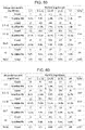
- FIG. 26 is a table illustrating Kalman Filter accuracy metrics.
- FIG. 27 is a table illustrating Kalman Filter regularity metrics.
- FIG. 28 is a table illustrating ROC accuracy with respect to the concurrence of CGM and YSI trends.
- FIG. 29 is a table illustrating ROC accuracy with respect to the concurrence of filtered CGM and YSI trends.
- FIGS. 30A-30C are graphs illustrating estimated error variance day-by-day (line with circles) with sensor's mean (dashed line) and global mean error variance (solid line), for three different sensors.
- FIGS. 31A-31D are graphs illustrating CGM data (thick line) versus smoothed signal (thin line) during a first time window, with weighted residuals (circles) during the first time window, CGM data (thick line) versus smoothed signal (thin line) during a second time window, and weighted residuals (circles) during the second time window, respectively, for a representative sensor.
- FIGS. 32A-32C are graphs illustrating CGM data (thin line) VS KF series (thick line) for a representative sensor during three different time windows.
- FIGS. 33A-33C are graphs illustrating CGM data (thin line) VS KF series (thick line) for a representative sensor during three different time periods.
- FIGS. 35A-35C are graphs illustrating KF series with time-varying (thick line), global (thick dashed line) or sensor individualized (thin dashed line) parameters versus CGM data (thin line) for a representative sensor during three different time windows.
- FIG. 36 is a table showing Kalman Filter accuracy metrics.
- FIG. 37 is a table showing Kalman Filter regularity metrics.
- FIG. 38 is a table showing ROC accuracy with respect to concurrence of CGM and YSI trends.
- FIG. 39 is a table showing ROC accuracy with respect to concurrence of CGM and YSI trends.
- FIG. 43 is a table illustrating original versus predicted time-series performance.
- FIG. 44 is a table illustrating time delay and gain between original and predicted series, calculated with cross-correlation.
- FIG. 45 is a table illustrating time delay and gain between original and predicted series at threshold crossing.
- FIG. 46 is a table illustrating number of peaks, nadirs and hypoglycemic events.
- FIG. 47 is a table illustrating prediction versus YSI performance at clinical session.
- FIG. 48 is a table illustrating ROC accuracy with respect to the concurrence of POL(1) prediction and YSI trends.
- FIG. 49 is a table illustrating ROC accuracy with respect to the concurrence of AR(1) prediction and YSI trends.
- FIG. 50 is a table illustrating ROC accuracy with respect to the concurrence of S prediction and YSI trends.
- FIG. 54 is table showing original VS predicted time-series performance.
- FIG. 55 is table showing time delay and gain between original and predicted series, calculated with cross-correlation.
- FIG. 56 is table showing time delay and gain between original and predicted series at threshold crossing.
- FIG. 57 is table showing a number of peaks, nadirs and hypoglycemic events.
- FIG. 58 is table showing prediction versus YSI performance at clinical session.
- FIG. 59 is table showing ROC accuracy with respect to the concurrence of POL(1) prediction and YSI trends.
- FIG. 60 is table showing ROC accuracy with respect to the concurrence of AR(1) prediction and YSI trends.
- FIG. 61 is table showing ROC accuracy with respect to the concurrence of S prediction and YSI trends.
- FIG. 62 is a table showing baseline characteristics.
- FIG. 63 is a table showing in-exclusive criteria.
- FIG. 64 is a table showing PRECISE study Dataset 1 information.
- FIG. 65 is a table showing PRECISE study Dataset 2 information.
- CGM data can open the doors to the realization of investigations and applications that were hindered by the sparseness of SMBG measurements.
- Retrospective data analysis of CGM readings can be very useful in tuning/refining diabetes therapy.
- a natural application of CGM devices concerns with the early detection of hypo/hyperglycemic episodes. For instance, by comparing the currently measured (or predicted ahead of time) glucose level with a given hypo/hyper threshold, an alert could be generated.
- CGM sensors are a key element of Artificial Pancreas (AP) research prototypes, i.e., minimally invasive systems for subcutaneous insulin infusion driven by a closed-loop control algorithm.
- AP Artificial Pancreas
- some analyte monitoring systems may include a long-term sensor (e.g., a fully subcutaneously long-term implantable sensor that uses a fluorescent, non-enzymatic (such as bisboronic acid based) glucose indicating hydrogel and a miniaturized optical detection system).
- the analyte monitoring system may include use a single sensor for continuous display of accurate analyte values for three months, even up to six months.
- the performance of the analyte monitoring system may still be suboptimal in terms of accuracy and precision.
- a “smart sensor” architecture concept that consists of an analyte sensor and circuitry configured to perform one or more of denoising, signal enhancement, and prediction has been developed.
- the present invention has the aim of improving the performance and the accuracy of analyte monitoring systems.
- the content is organized as follows. Section 1 describes briefly what diabetes is, and how it can be controlled through CGM devices. In Section 2, an analyte monitoring system is widely described, while in Section 3 the database used is presented. In Sections 4 and 5, methods, implementation notes and results of, respectively, denoising and prediction analyses are explained.
- glucose metabolism is fundamental both from a physiological point of view, because glucose is the main source of energy for the whole body cells, and from a pathological point of view, because a malfunction of this system would lead to phenomena of glucose intolerance or, in the worst case, to diabetes.
- concentration of glucose in healthy subjects is tightly regulated by a complex neuro-hormonal control system.
- Insulin which is secreted by the ⁇ -cells of the pancreas, is the primary regulator of glucose homeostasis, by promoting its use by tissues and inhibiting its endogenous production.
- hormones such as glucagon, epinephrine, cortisol, and growth hormone play the role, on different time scales, to prevent hypoglycemia.
- Glucose is generally absorbed by the gastro-intestinal tract through food digestion after a meal or, in fasting condition, it is provided primarily by the liver. Glucose is distributed and used in the whole body. Based on the specific needs and roles in its regulation, tissues and organs can be classified as (i) insulin-independent, (ii) insulin-dependent, and (iii) gluco-sensors. In insulin-independent tissues and organs, such as the central nervous system and erythrocytes, glucose is the substrate of choice and its extraction takes place at a constant speed, regardless of insulin concentration.
- glucose-dependent tissues and organs such as muscle, adipose tissue and liver
- the utilization of glucose by these tissues is phasic; in fact, it is modulated by the amount of circulating insulin.
- Gluco-sensors such as pancreas ⁇ -cells, the liver, and the hypothalamus, are sensitive to glucose concentration and could provide a proper secretory response.
- FIG. 1 a schematic representation of the glucose-insulin control system is shown.
- the production of glucose mainly provided by the liver and its utilization, mediated and not by insulin action, is shown.
- the secretion of insulin from of the ⁇ -cells and its degradation by tissues are shown.
- Dashed arrows show the mutual control between glucose and insulin, where insulin promotes glucose utilization and inhibits its production, while glucose stimulates insulin secretion.
- the control system is in closed loop form: glucose stimulates insulin secretion and this, in turn, acts on glucose production and utilization. An imbalance of this feedback control system can lead to diseases such as diabetes.
- Diabetes is a chronic disease characterized by either an autoimmune destruction of pancreas ⁇ -cells, leading to insulin deficiency (Type 1 Diabetes Mellitus, T1DM), or by insulin resistance (Type 2 Diabetes Mellitus, T2DM) which may be combined with impaired insulin secretion.
- Type 1 Diabetes Mellitus, T1DM Type 1 Diabetes Mellitus
- Type 2 Diabetes Mellitus, T2DM insulin resistance
- T1DM Type 1 Diabetes Mellitus
- T2DM insulin resistance
- impaired insulin secretion Type 2 Diabetes Mellitus
- Type 1 diabetes is the form of diabetes that results from autoimmune destruction of insulin-producing ⁇ -cells of the pancreas.
- the insulin deficiency results in the inability of cells (in particular fat and muscle) to utilize and store glucose, with immediate consequences. These consequences include (i) accumulation of glucose in plasma which leads to strong hyperglycemia, to exceed the threshold of renal reabsorption causing glycosuria, polyuria and polydipsia, and (ii) use of alternative sources of energy such as the lipid reserves, bringing the loss of body fat and protein reserves with loss of lean body mass.
- Type 1 diabetes is less than 10% of cases of diabetes and it is a disease of childhood thus affecting mostly children and adolescents, more rarely young adults (90% ⁇ 20 years).
- Type 2 diabetes is characterized by three physiological abnormalities: impaired insulin secretion, insulin resistance, and overproduction of endogenous glucose. It is the most common type of diabetes (more than 90% of cases), and it is a typically disease of mature age (>40 years), even if it starts to affect patients getting younger.
- the pathogenesis of type 2 diabetes is caused by a combination of lifestyle (obesity, lack of physical activity, etc.) and genetic factors. This form of diabetes frequently goes undiagnosed for many years because the hyperglycemia develops gradually and at earlier stages it is often not severe enough for the patient to notice any of the classic symptoms of diabetes.
- Insulin resistance may improve with weight reduction and/or pharmacological treatment of hyperglycemia but is seldom restored to normal.
- diabetes all forms of diabetes increase the risk of long-term complications, which are mainly related to damage to blood vessels. In fact, diabetes doubles the risk of cardiovascular disease.
- the main “macrovascular” diseases (related to atherosclerosis of larger arteries) are ischemic heart disease (angina and myocardial infarction), stroke and peripheral vascular disease.
- ischemic heart disease angina and myocardial infarction
- stroke and peripheral vascular disease While the main “microvascular” complications (damage to the small blood vessels) are: (i) diabetic retinopathy, (ii) diabetic nephropathy, (iii) and diabetic neuropathy.
- Diabetic retinopathy (70% T1DM, 40% T2DM) affects blood vessel formation in the retina of the eye, leading to visual symptoms, reduced vision, and potentially blindness.
- Diabetic neuropathy With diabetic nephropathy (20-30% of diabetic patients), the impact of diabetes on the kidneys can lead to scarring changes in the kidney tissue, loss of small or progressively larger amounts of protein in the urine, and eventually chronic kidney disease requiring dialysis. Diabetic neuropathy (20-40% of diabetic patients) is the impact of diabetes on the nervous system, most commonly causing numbness, tingling and pain in the feet and also increasing the risk of skin damage due to altered sensation. Together with vascular disease in the legs, neuropathy contributes to the risk of diabetes-related foot problems (such as diabetic foot ulcers) that can be difficult to treat and occasionally require amputation.
- diabetes-related foot problems such as diabetic foot ulcers
- Short-term complications may be caused by either hypoglycemia or hyperglycemia.
- the first case occurs in people with diabetes treated with insulin or hypoglycemic agents and is more common in people who miss or delay meals after an insulin bolus or do physical activity unexpectedly, causing an increase in glucose utilization by tissues.
- the second case diabetic ketoacidosis, occurs usually in young people with type 1 diabetes, and the main cause is the absolute or relative deficiency of insulin.
- cerebral edema hyperchloremic acidosis, lactic acidosis, infections, gastric dilation, erosion and thromboembolism.
- hyperglycemic-hyperosmolar syndrome characterized by hyperosmolarity (plasma osmolality>320 mosm/kg), severe hyperglycemia (blood glucose>600 mg/dl), marked dehydration, the absence of acidosis.
- SMBG values are not sufficient to identify episodes of post-prandial hyperglycemia and especially those of hypoglycemia caused by an overdose of insulin.
- invasiveness minimally invasive or non-invasive.
- CGM Continuous Glucose Monitoring
- the standard treatment for patients with diabetes is therefore based on multiple daily injections of insulin (bolus and basal doses), diet and exercise, tuned according to self-monitoring of blood glucose (SMBG) levels 3 to 4 times a day. Thanks to the availability of CGM sensors and insulin delivery systems has been possible to improve the management of diabetes.
- SMBG blood glucose
- the SMBG however is still remained fundamental for control therapy due to possible systematic and random errors of CGM sensors, becoming of considerable importance the calibration procedure enabled by SMBG values.
- FIG. 2 Comparison between glycemic profiles obtained with SMBG (filled circles) and CGM (continuous line)
- the first CGM systems offered only an “offline” interpretation of the glucose profiles after disconnecting the sensor and uploading the results.
- glucose monitoring devices in: (i) minimally invasive sensors (e.g., with systems of micro dialysis, based on ionophoresis, or based on electrochemistry), (ii) non-invasive sensors (e.g., based on spectroscopy or based on light scattering), and (iii) totally implantable glucose sensors (e.g., intravascular or subcutaneous).
- minimally invasive sensors e.g., with systems of micro dialysis, based on ionophoresis, or based on electrochemistry
- non-invasive sensors e.g., based on spectroscopy or based on light scattering
- totally implantable glucose sensors e.g., intravascular or subcutaneous.
- embodiments of the invention are applicable to analyte monitoring systems including different types of analyte sensors.
- FIG. 3 is a schematic view of an analyte monitoring system 1 embodying aspects of the present invention.
- the analyte monitoring system 1 may be a continuous analyte monitoring system (e.g., a CGM system).
- the analyte monitoring system 1 may include one or more of an analyte sensor 100 , a transmitter 101 , and a display device 105 .
- the sensor 100 may be small, fully subcutaneously insertable sensor measures analyte (e.g., glucose) concentrations in a medium (e.g., interstitial fluid) of a living animal (e.g., a living human).
- analyte e.g., glucose
- the senor 100 may be a partially insertable (e.g, transcutaneous) sensor or a fully external sensor.
- the transmitter 101 may be an externally worn transmitter (e.g., attached via an armband, wristband, waistband, or adhesive patch).
- the transmitter 101 may remotely power and communicate with the inserted sensor to initiate and receive the measurements (e.g., via near field communication).
- the transmitter 101 may power and/or communicate with the sensor 100 via one or more wired connections.
- the transmitter 101 may communicate information (e.g., one or more analyte concentrations) wirelessly (e.g., via a BluetoothTM communication standard such as, for example and without limitation Bluetooth Low Energy) to a hand held application running on a display device 105 (e.g., smartphone).
- information can be downloaded from the transmitter 101 through a Universal Serial Bus (USB) port.
- the analyte monitoring system 1 may include a web interface for plotting and sharing of uploaded data.
- the transmitter 101 may include an inductive element 103 , such as, for example, a coil.
- the transmitter 101 may generate an electromagnetic wave or electrodynamic field (e.g., by using a coil) to induce a current in an inductive element 114 of the sensor 100 , which powers the sensor 100 .
- the transmitter 101 may also convey data (e.g., commands) to the sensor 100 .
- the transmitter 101 may convey data by modulating the electromagnetic wave used to power the sensor 100 (e.g., by modulating the current flowing through a coil 103 of the transmitter 101 ).
- the modulation in the electromagnetic wave generated by the transmitter 101 may be detected/extracted by the sensor 100 .
- the transmitter 101 may receive data (e.g., measurement information) from the sensor 100 .
- the transmitter 101 may receive data by detecting modulations in the electromagnetic wave generated by the sensor 100 , e.g., by detecting modulations in the current flowing through the coil 103 of the transmitter 101 .
- the inductive element 103 of the transmitter 101 and the inductive element 114 of the sensor 100 may be in any configuration that permits adequate field strength to be achieved when the two inductive elements are brought within adequate physical proximity.
- the senor 100 may be encased in a sensor housing 102 (i.e., body, shell, capsule, or encasement), which may be rigid and biocompatible.
- the sensor 100 may include an analyte indicator element 106 , such as, for example, a polymer graft coated, diffused, adhered, or embedded on or in at least a portion of the exterior surface of the sensor housing 102 .
- the analyte indicator element 106 (e.g., polymer graft) of the sensor 100 may include indicator molecules 104 (e.g., fluorescent indicator molecules) exhibiting one or more detectable properties (e.g., optical properties) based on the amount or concentration of the analyte in proximity to the analyte indicator element.
- the sensor 100 may include a light source 108 that emits excitation light 329 over a range of wavelengths that interact with the indicator molecules 104 .
- the sensor 100 may also include one or more photodetectors 224 , 226 (e.g., photodiodes, phototransistors, photoresistors, or other photosensitive elements).
- the one or more photodetectors may be sensitive to emission light 331 (e.g., fluorescent light) emitted by the indicator molecules 104 such that a signal generated by a photodetector (e.g., photodetector 224 ) in response thereto that is indicative of the level of emission light 331 of the indicator molecules and, thus, the amount of analyte of interest (e.g., glucose).
- emission light 331 e.g., fluorescent light
- a signal generated by a photodetector e.g., photodetector 224
- the photodetectors e.g., photodetector 226
- one or more of the photodetectors may be covered by one or more filters that allow only a certain subset of wavelengths of light to pass through (e.g., a subset of wavelengths corresponding to emission light 331 or a subset of wavelengths corresponding to reflection light 333 ) and reflect the remaining wavelengths.
- the sensor 100 may include a temperature transducer 670 .
- the sensor 100 may include a drug-eluting polymer matrix that disperses one or more therapeutic agents (e.g., an anti-inflammatory drug).
- the sensor 100 may include a substrate 116 .
- the substrate 116 may be a circuit board (e.g., a printed circuit board (PCB) or flexible PCB) on which circuit components (e.g., analog and/or digital circuit components) may be mounted or otherwise attached.
- the substrate 116 may be a semiconductor substrate having circuitry fabricated therein.
- the circuitry may include analog and/or digital circuitry.
- circuitry in addition to the circuitry fabricated in the semiconductor substrate, circuitry may be mounted or otherwise attached to the semiconductor substrate 116 .
- a portion or all of the circuitry which may include discrete circuit elements, an integrated circuit (e.g., an application specific integrated circuit (ASIC)) and/or other electronic components (e.g., a non-volatile memory), may be fabricated in the semiconductor substrate 116 with the remainder of the circuitry is secured to the semiconductor substrate 116 and/or a core (e.g., ferrite core) for the inductive element 114 .
- the semiconductor substrate 116 and/or a core may provide communication paths between the various secured components.
- the one or more of the sensor housing 102 , analyte indicator element 106 , indicator molecules 104 , light source 108 , photodetectors 224 , 226 , temperature transducer 670 , substrate 116 , and inductive element 114 of sensor 100 may include some or all of the features described in one or more of U.S. application Ser. No. 13/761,839, filed on Feb. 7, 2013, U.S. application Ser. No. 13/937,871, filed on Jul. 9, 2013, and U.S. application Ser. No. 13/650,016, filed on Oct. 11, 2012, all of which are incorporated by reference in their entireties.
- the structure and/or function of the sensor 100 and/or transmitter 101 may be as described in one or more of U.S. application Ser. Nos. 13/761,839, 13/937,871, and 13/650,016.
- the senor 100 may be an optical sensor, this is not required, and, in one or more alternative embodiments, sensor 100 may be a different type of analyte sensor, such as, for example, a diffusion sensor or a pressure sensor. Also, although in some embodiments, as illustrated in FIGS. 3 and 4 , the analyte sensor 100 may be a fully implantable sensor, this is not required, and, in some alternative embodiments, the sensor 100 may be a transcutaneous sensor having a wired connection to the transmitter 101 . For example, in some alternative embodiments, the sensor 100 may be located in or on a transcutaneous needle (e.g., at the tip thereof).
- the senor 100 and transmitter 101 may communicate using one or more wires connected between the transmitter 101 and the transmitter transcutaneous needle that includes the sensor 100 .
- the sensor 100 may be located in a catheter (e.g., for intravenous blood glucose monitoring) and may communicate (wirelessly or using wires) with the transmitter 101 .
- the sensor 100 may include a transmitter interface device.
- the transmitter interface device may include the antenna (e.g., inductive element 114 ) of sensor 100 .
- the transmitter interface device may include the wired connection.
- FIGS. 5 and 6 are cross-sectional and exploded views, respectively, of a non-limiting embodiment of the transmitter 101 , which may be included in the analyte monitoring system illustrated in FIGS. 3 and 4 .
- the transmitter 101 may include a graphic overlay 204 , front housing 206 , button 208 , printed circuit board (PCB) assembly 210 , battery 212 , gaskets 214 , antenna 103 , frame 218 , reflection plate 216 , back housing 220 , ID label 222 , and/or vibration motor 928 .
- PCB printed circuit board
- the vibration motor 928 may be attached to the front housing 206 or back housing 220 such that the battery 212 does not dampen the vibration of vibration motor 928 .
- the transmitter electronics may be assembled using standard surface mount device (SMD) reflow and solder techniques.
- the electronics and peripherals may be put into a snap together housing design in which the front housing 206 and back housing 220 may be snapped together.
- the full assembly process may be performed at a single external electronics house. However, this is not required, and, in alternative embodiments, the transmitter assembly process may be performed at one or more electronics houses, which may be internal, external, or a combination thereof.
- the assembled transmitter 101 may be programmed and functionally tested. In some embodiments, assembled transmitters 101 may be packaged into their final shipping containers and be ready for sale.
- the antenna 103 may be contained within the housing 206 and 220 of the transmitter 101 .
- the antenna 103 in the transmitter 101 may be small and/or flat so that the antenna 103 fits within the housing 206 and 220 of a small, lightweight transmitter 101 .
- the antenna 103 may be robust and capable of resisting various impacts.
- the transmitter 101 may be suitable for placement, for example, on an abdomen area, upper-arm, wrist, or thigh of a patient body.
- the transmitter 101 may be suitable for attachment to a patient body by means of a biocompatible patch.
- the antenna 103 may be contained within the housing 206 and 220 of the transmitter 101 , this is not required, and, in some alternative embodiments, a portion or all of the antenna 103 may be located external to the transmitter housing.
- antenna 103 may wrap around a user's wrist, arm, leg, or waist such as, for example, the antenna described in U.S. Pat. No. 8,073,548, which is incorporated herein by reference in its entirety.
- FIG. 7 is a schematic view of an external transmitter 101 according to a non-limiting embodiment.
- the transmitter 101 may have a connector 902 , such as, for example, a Micro-Universal Serial Bus (USB) connector.
- the connector 902 may enable a wired connection to an external device, such as a personal computer (e.g., personal computer 109 ) or a display device 105 (e.g., a smartphone).
- a personal computer e.g., personal computer 109
- a display device 105 e.g., a smartphone
- the transmitter 101 may exchange data to and from the external device through the connector 902 and/or may receive power through the connector 902 .
- the transmitter 101 may include a connector integrated circuit (IC) 904 , such as, for example, a USB-IC, which may control transmission and receipt of data through the connector 902 .
- the transmitter 101 may also include a charger IC 906 , which may receive power via the connector 902 and charge a battery 908 (e.g., lithium-polymer battery).
- the battery 908 may be rechargeable, may have a short recharge duration, and/or may have a small size.
- the transmitter 101 may include one or more connectors in addition to (or as an alternative to) Micro-USB connector 904 .
- the transmitter 101 may include a spring-based connector (e.g., Pogo pin connector) in addition to (or as an alternative to) Micro-USB connector 904 , and the transmitter 101 may use a connection established via the spring-based connector for wired communication to a personal computer (e.g., personal computer 109 ) or a display device 105 (e.g., a smartphone) and/or to receive power, which may be used, for example, to charge the battery 908 .
- a spring-based connector e.g., Pogo pin connector
- the transmitter 101 may use a connection established via the spring-based connector for wired communication to a personal computer (e.g., personal computer 109 ) or a display device 105 (e.g., a smartphone) and/or to receive power, which may be used, for example, to charge the battery 908 .
- a personal computer e.
- the transmitter 101 may have a wireless communication IC 910 , which enables wireless communication with an external device, such as, for example, one or more personal computers (e.g., personal computer 109 ) or one or more display devices 105 (e.g., a smartphone).
- the wireless communication IC 910 may employ one or more wireless communication standards to wirelessly transmit data.
- the wireless communication standard employed may be any suitable wireless communication standard, such as an ANT standard, a Bluetooth standard, or a Bluetooth Low Energy (BLE) standard (e.g., BLE 4 . 0 ).
- the wireless communication IC 910 may be configured to wirelessly transmit data at a frequency greater than 1 gigahertz (e.g., 2.4 or 5 GHz).
- the wireless communication IC 910 may include an antenna (e.g., a Bluetooth antenna).
- the antenna of the wireless communication IC 910 may be entirely contained within the housing (e.g., housing 206 and 220 ) of the transmitter 101 . However, this is not required, and, in alternative embodiments, all or a portion of the antenna of the wireless communication IC 910 may be external to the transmitter housing.
- the transmitter 101 may include a display interface device, which may enable communication by the transmitter 101 with one or more display devices 105 .
- the display interface device may include the antenna of the wireless communication IC 910 and/or the connector 902 .
- the display interface device may additionally include the wireless communication IC 910 and/or the connector IC 904 .
- the transmitter 101 may include voltage regulators 912 and/or a voltage booster 914 .
- the battery 908 may supply power (via voltage booster 914 ) to radio-frequency identification (RFID) reader IC 916 , which uses the inductive element 103 to convey information (e.g., commands) to the sensor 101 and receive information (e.g., measurement information) from the sensor 100 .
- RFID radio-frequency identification
- the sensor 100 and transmitter 101 may communicate using near field communication (NFC) (e.g., at a frequency of 13.56 MHz).
- NFC near field communication
- the inductive element 103 is a flat antenna.
- the antenna may be flexible.
- the inductive element 103 of the transmitter 101 may be in any configuration that permits adequate field strength to be achieved when brought within adequate physical proximity to the inductive element 114 of the sensor 100 .
- the transmitter 101 may include a power amplifier 918 to amplify the signal to be conveyed by the inductive element 103 to the sensor 100 .
- the transmitter 101 may include a peripheral interface controller (PIC) microcontroller 920 and memory 922 (e.g., Flash memory), which may be non-volatile and/or capable of being electronically erased and/or rewritten.
- PIC microcontroller 920 may control the overall operation of the transmitter 101 .
- the PIC microcontroller 920 may control the connector IC 904 or wireless communication IC 910 to transmit data via wired or wireless communication and/or control the RFID reader IC 916 to convey data via the inductive element 103 .
- the PIC microcontroller 920 may also control processing of data received via the inductive element 103 , connector 902 , or wireless communication IC 910 .
- the transmitter 101 may include a sensor interface device, which may enable communication by the transmitter 101 with a sensor 100 .
- the sensor interface device may include the inductive element 103 .
- the sensor interface device may additionally include the RFID reader IC 916 and/or the power amplifier 918 .
- the sensor interface device may include the wired connection.
- the transmitter 101 may include a display 924 (e.g., liquid crystal display and/or one or more light emitting diodes), which PIC microcontroller 920 may control to display data (e.g., glucose concentration values).
- the transmitter 101 may include a speaker 926 (e.g., a beeper) and/or vibration motor 928 , which may be activated, for example, in the event that an alarm condition (e.g., detection of a hypoglycemic or hyperglycemic condition) is met.
- the transmitter 101 may also include one or more additional sensors 930 , which may include an accelerometer and/or temperature sensor, that may be used in the processing performed by the PIC microcontroller 920 .
- the transmitter 101 may be a body-worn transmitter that is a rechargeable, external device worn over the sensor implantation or insertion site.
- the transmitter 101 may supply power to the proximate sensor 100 , calculate analyte concentrations from data received from the sensor 100 , and/or transmit the calculated analyte concentrations to a display device 105 (see FIG. 3 ).
- Power may be supplied to the sensor 100 through an inductive link (e.g., an inductive link of 13.56 MHz).
- the transmitter 101 may be placed using an adhesive patch or a specially designed strap or belt.
- the external transmitter 101 may read measured analyte data from a subcutaneous sensor 100 (e.g., up to a depth of 2 cm or more).
- the transmitter 101 may periodically (e.g., every 2 minutes) read sensor data and calculate an analyte concentration and an analyte concentration trend. From this information, the transmitter 101 may also determine if an alert and/or alarm condition exists, which may be signaled to the user (e.g., through vibration by vibration motor 928 and/or an LED of the transmitter's display 924 and/or a display of a display device 105 ).
- an alert and/or alarm condition exists, which may be signaled to the user (e.g., through vibration by vibration motor 928 and/or an LED of the transmitter's display 924 and/or a display of a display device 105 ).
- the information from the transmitter 101 may be transmitted to a display device 105 (e.g., via Bluetooth Low Energy with Advanced Encryption Standard (AES)-Counter CBC-MAC (CCM) encryption) for display by a mobile medical application on the display device 105 .
- the mobile medical application may provide alarms, alerts, and/or notifications in addition to any alerts, alarms, and/or notifications received from the transmitter 101 .
- the mobile medical application may be configured to provide push notifications.
- the transmitter 101 may have a power button (e.g., button 208 ) to allow the user to turn the device on or off, reset the device, or check the remaining battery life.
- the transmitter 101 may have a button, which may be the same button as a power button or an additional button, to suppress one or more user notification signals (e.g., vibration, visual, and/or audible) of the transmitter 101 generated by the transmitter 101 in response to detection of an alert or alarm condition.
- a power button e.g., button 208
- the transmitter 101 may have a button, which may be the same button as a power button or an additional button, to suppress one or more user notification signals (e.g., vibration, visual, and/or audible) of the transmitter 101 generated by the transmitter 101 in response to detection of an alert or alarm condition.
- the senor 100 may be a micro-fluorometer that is encased in a rigid, translucent, and/or biocompatible polymer capsule (e.g., PMMA) 102 .
- the capsule 102 may be, for example and without limitation, 3.3 mm in diameter and 15 mm in length.
- analyte concentration may be measured by means of fluorescence from the indicator element 106 (e.g., the analyte-indicating hydrogel), which may be, for example and without limitation, polymerized onto the capsule surface over the optical cavity.
- the indicator element 106 e.g., the analyte-indicating hydrogel
- the optical system contained within the capsule 102 may include one or more of a light-emitting diode (LED) 108 , which may serve as the excitation source for the indicator element 106 ; one or more photodetectors 224 and 226 , which may be, for example and without limitation, spectrally filtered photodiodes, which may measure the analyte-dependent fluorescence intensity; circuitry (e.g., a custom integrated circuit with onboard temperature sensor); an on-board nonvolatile storage medium (e.g., an electrically erasable programmable memory (EEPROM)), which may be for local configuration storage and/or production traceability; and an antenna 114 , which may receive power from and communicates with the transmitter 101 .
- LED light-emitting diode
- photodetectors 224 and 226 which may be, for example and without limitation, spectrally filtered photodiodes, which may measure the analyte-dependent fluorescence intensity
- circuitry e.g.
- FIGS. 8A-8C illustrate an implantable optical-based glucose sensor.
- FIG. 8A is a photograph of the implantable glucose sensor (shown without glucose-indicator hydrogel coating);
- FIG. 8B shows scanning electron microscope (SEM) images of the glucose indicator hydrogel grafted onto the outside of the PMMA sensor encasement;
- FIG. 8C shows a chemical structure and glucose binding mode of indicator moiety.
- R 2 shown in the figure denotes connectivity to the hydrogel backbone, while R 1 represents a propionic acid side chain.
- the analyte indicator 106 may include poly(2-hydroxyethyl methacrylate) (pHEMA) into which a fluorescent indicator ( FIG. 8C ) may be co-polymerized.
- pHEMA poly(2-hydroxyethyl methacrylate)
- FIG. 8C a fluorescent indicator
- glucose-indicating hydrogel in contrast to CGMs that utilize electrochemical enzyme-based glucose sensors, no chemical compounds are consumed (i.e., glucose, oxygen) or formed (i.e., hydrogen peroxide) during use, and the glucose-indicating hydrogel may not subject to the instability characteristics of enzymes. Instead, glucose may reversibly binds to the indicator boronic acids groups (which act as glucose receptors) in an equilibrium binding reaction.
- PTT photoinduced electron transfer
- anthracene fluorescence may be quenched by intermolecular electron transfer (indicated by the curved arrows in FIG. 8C ) from the unpaired electrons on the indicator tertiary amines.
- intermolecular electron transfer indicated by the curved arrows in FIG. 8C
- the Lewis acidity of boron may be increased, and weak boron-nitrogen bonds are formed. This weak bonding may prevent electron transfer from the amines and may consequently prevent fluorescence quenching.
- the indicator is not chemically altered as a result of the PET quenching process.
- an anti-oxidant layer e.g., platinum
- a glucose-permeable membrane may cover the analyte indicator 106 (e.g., hydrogel) and may provide a biocompatible interface.
- the ability of the sensor 100 to communicate may be mediated by a near field communication (NFC) interface to the external transmitter 101 .
- NFC near field communication
- the sensor 100 may not contain a battery or other stored power source; instead, the sensor 100 may be remotely and discretely powered, as needed, by a simple inductive magnetic link between the sensor and the transmitter 101 .
- the LED source 108 may be energized (e.g., for approximately 4 ms) to excite the fluorescent indicator. Between readings, the sensor 100 may remain electrically dormant and fully powered down.
- the body-worn transmitter 101 may be a rechargeable, external device that is worn over the sensor implantation site and that supplies power to the proximate sensor 100 , calculates glucose concentration from data received from the sensor, and/or transmits the glucose calculation to a smartphone 105 .
- the transmitter 101 may supply power to the sensor 100 through an inductive link (e.g., of 13.56 MHz).
- the transmitter 101 may be placed using an adhesive patch or band (i.e., armband, waistband, and wristband).
- the transmitter 101 may power and activate a measurement sequence (e.g., every 2 min), read measured glucose data from the sensor 100 (e.g., up to a depth of approximately 2-3 cm) and then calculate glucose concentrations and/or trends.
- This information may also enable the transmitter 101 to determine if an alert condition exists, which may be communicated to the wearer through vibration and/or the transmitter's display 924 .
- the information from the transmitter 101 may then transmitted for display to a smartphone 105 (e.g., via a BluetoothTM low energy link).
- the analyte monitoring system 1 may include one or more of three different phases: Warm up, Initialization, and Calibration phases.
- the sensor 100 may be inserted into the subcutaneous space (e.g., using aseptic technique via a small incision ( ⁇ 0.8-1.0 cm) made under local anesthesia with lidocaine). Two 5-0 nylon sutures may be used to close the wound. A typical insertion time may be less than 5 min.
- the transmitter 101 and the application may be paired, and the sensor 100 and the transmitter 101 linked. Then, the Warm up phase may begin (e.g., day 0, 24 h after insertion), in which the transmitter 101 is not worn, and no calibration is done.
- each SMBG measurement entry may be, for example, 2-12 hours apart.
- the Daily calibration phase begins, and one or more (e.g., two) SMBG measurements entries per time period (e.g., day or week) may be done.
- each SMBG measurement entry may be 10-14 hours apart, and the system 1 may allow preferred daily calibration times to be set by patient, e.g., 08:00 and 18:00.
- the removal of the sensor 100 e.g., upon completion of a study or end of sensor life
- aseptic techniques e.g., under local anesthesia with lidocaine.
- a small incision may be made at the proximal end of the sensor location, and manual pressure may be applied to the distal end to extrude the sensor from the subcutaneous space through the incision.
- a thin adhesive strip or suture may be applied to assure closure at the removal site. Typical excision times may be less than 5 min.
- the analyte monitoring system 1 may be configured to perform one or more of the functions illustrated in FIG. 9 .
- the transmitter 101 e.g., the microcontroller 920 of the transmitter 101
- the sensor 100 e.g., circuitry, such as an ASIC, of the sensor 100
- the sensor 100 may be configured to perform one or more of the functions illustrated in FIG. 9 .
- the sensor 100 may measure one or more of the raw fluorescent signal (e.g., emission light 331 ), the reference signal (e.g., reflection light 333 ), and the temperature of the sensor 100 . In some embodiments, the sensor 100 may convey the measurement information to the transmitter 101 . In some embodiments, the analyte monitoring system 1 (e.g., the transmitter 101 of the analyte monitoring system 1 ) may store one or more parameters measured during manufacturing of the sensor 101 and/or one or more parameters characterized using in-vitro and/or in-vivo tests.
- the raw fluorescent signal e.g., emission light 331
- the reference signal e.g., reflection light 333
- the sensor 100 may convey the measurement information to the transmitter 101 .
- the analyte monitoring system 1 e.g., the transmitter 101 of the analyte monitoring system 1
- the analyte monitoring system 1 may generate a much purified signal derived from glucose modulated indicator fluorescence that is normalized (Sn) and directly proportional to glucose concentration.
- the two different measurement channels (signal and reference) of the sensor 100 may be used to calculate the normalized signal.
- This normalized signal may contain some parameters that have to be calibrated, for a good performance of the system 1 .
- This calibration may be done using one or more SMBG measurements, which the system 1 may receive, for example and without limitation, via patient entry into the hand held application of display device 105 , which may convey the one or more SMBG measurements to the transmitter 101 .
- the calibration evaluate an acceptance criterion.
- the system 1 may accept it. If not, the system 1 may be configured to treat the SMBG value as wrong, thus having to change its behavior. In some embodiments, the system 1 may be configured to perform an interpretive algorithm that modifies the normalized signal Sn into an interstitial gel glucose concentration. In some embodiments, the analyte monitoring system 1 may be configured to transform the interstitial gel glucose concentration into a real blood glucose concentration (e.g., by a lag compensation algorithm).
- the system 1 may generate other outputs, like sensor performance and accuracy metrics as the Metric for real time assessment of Sensor Performance (MSP), the Metric of Electronic Performance (MEP), the Mean Absolute Relative Difference (MARD), and/or trend value and alarms prediction.
- MSP Sensor Performance
- MEP Metric of Electronic Performance
- MARD Mean Absolute Relative Difference
- the signal-processing cascade performed by the analyte monitoring system 1 may be based on the relationship shown in FIG. 10 .
- I is the fluorescence from the glucose sensor indicator and I 0 is baseline fluorescence at zero glucose concentration.
- the percent modulation I/I 0 versus glucose concentration is constant throughout the life of the glucose sensor (indicator).
- the end of life of the analyte sensor 100 may arise when the signal to noise ratio declines over time to a point where the error specification can no longer be maintained.
- the system 1 may use an interpretive algorithm to convert Sn into glucose concentration. This algorithm may be derived through the curve seen in FIG. 10 . This curve may be based on the equilibrium reaction: Indicator+Glucose Indicator_Glucose_Complex (2.1)
- the fluorescence of the indicator may increase upon binding glucose.
- the analyte monitoring system 1 may purify and transform this fluorescent signal, which may be directly proportional to glucose concentration, to obtain the desired blood glucose concentration.
- the raw signals from the sensor 100 may contain noise, offset, and/or distortions, which are not related to actual glucose modulation of the indicator 106 .
- the fluorescent amplitude of the indicator 106 may be temperature sensitive.
- the analyte monitoring system 1 may use the Sn equation to purify and normalize the signal by removing the non-glucose-modulated offset/distortion of the signal, and/or may correct for temperature sensitivity.
- the simplest form of Sn equation is that
- FIG. 11 Reactions and kinetics
- the excitation light 329 emitted from light source 108 that reaches the photodetector may include (i) a reflection light component 335 that is reflected from the graft 106 (e.g., gel) before reaching the photodetector and (ii) a bleed light component 337 that reaches the photodetector without encountering the graft 106 .
- the reflection light component 335 may produce a reflection component Z gel of the offset Z
- the bleed light component 337 may produce a bleed component Z bleed of the offset Z.
- the offset (Z) may be hardware based, due to LED light that is not absorbed by the indicator 106 , mostly because it did not encounter an indicator molecule 104 . That light (offset) is then removed by Sn equation, since it is convoluted in the total light arriving at the photodetector.
- the offset may be measured during the manufacturing of the sensor 100 , and the offset may increase due to photo-bleaching (i.e., the fluorescent reagents “shutdown” reaction).
- the Sn equation may dynamically track the offset, with the reference channel photodiode.
- Zgel is the LED spillover component 335 which is reflected from the gel (graft) to the photodetector, while Zbleed is the component 337 directly detected from the photodetector.
- ⁇ Z is the percent increase of Zgel when the indicator is fully photo-bleached.
- the offset (Z) may be used to normalize each sensor's output to a numerical value equal to one at zero glucose concentration (Snmin).
- the system distortion is chemistry (photochemistry) and kinetics based.
- the distortion is any non-glucose-modulated light arriving at the photodetector.
- photo [PA], thermal [Th], and oxidative [Ox] decay species emit fluorescent light that is not modulated by glucose, as shown within FIG. 11 .
- These mechanisms cause the signal degradation, which establishes the end of useful life for the overall sensor product. They are all chronic and predictable under a first order decay function on the loss of signal amplitude.
- % FOx, % FTh and % FPA are the relative quantum efficiencies. Only modulated fluorescence, I, carries glucose concentration information within the system. The effect of not removing these noise sources would compress the modulation shown in FIG. 10 (i.e., the y-axis displacement from zero to infinite glucose).
- the Sn equation removes or compensates distortion-inducing factors such that the processed signal is normalized and a constant value at infinite glucose concentration (Snmax—asymptote as shown in FIG. 10 ). The Sn equation becomes:
- I0 I 0,QC GID[1 ⁇ ( T+ 37) c f ]
- GID e ⁇ k ox t ox e ⁇ k th t th e ⁇ k pb t pb
- I0,QC is I0 obtained from manufacturing quality control (QC).
- kox, kth, and kpb are rates for oxidation, thermal degradation and photo-bleaching, respectively.
- tox, tth and tpb are oxidation time, thermal degradation time and photo-bleaching time, respectively.
- cf is the temperature correction coefficient of glucose indicator.
- tpb is tracked by using the cumulative LED-On time
- tox and tth are the time since the sensor is implanted.
- GID is the glucose indicator decay due to the superimpose of oxidation, thermal degradation and photo-bleaching. It is configured within the algorithm to kinetically track the first order decay loss of signal that occurs over time.
- the distortion producing subspecies [Ox], [Th] and [PA]
- the distortion producing subspecies will form progressively and the analyte monitoring system 1 may kinetically track the fluorescence from each subspecies.
- the interpretive algorithm performed by the analyte monitoring system 1 may be based on the first principles constant base relationship between percent modulation and glucose as shown in FIG. 10 .
- the interpretive algorithm may be based on the reaction in the equilibrium equation (2.1) and may convert Sn into glucose concentration.
- F I e dce ⁇ (2.12) where F is fluorescence of the species, I e is excitation light, d is path length, c is concentration of fluorescer, e is molar excitation coefficient and ⁇ is quantum efficiency.
- F fluorescence of the species
- I e excitation light
- d path length
- c concentration of fluorescer
- e molar excitation coefficient
- ⁇ quantum efficiency.
- equation (2.13) becomes
- each sensor 100 may be cycled through a computer automated quality control measurement rig, which may measure one or more parameters (e.g., one or more of c z , K d , Sn max , Z gel , and Z bleed ).
- one or more other parameters may be developed from designed and controlled in-vitro experiments (e.g., one or more of K pb , K PA , K th , ⁇ Z , c f , c Th . c Ox , c PA , % F Ox , % F PA , and % F Th ) and in-vivo tests (e.g., K Ox ).
- the analyte monitoring system 1 may use an algorithm for real-time smoothing/filtering. Based on the signal-processing algorithm aforementioned, the raw sensor measurements may be converted into corresponding glucose values perceived at the hydrogel surface of the sensor, referred to as Gel glucose, and then the glucose levels in the blood may be inferred based on an in-vivo venous-to-glucose indicator diffusion model and/or an in-vivo sensor sensitivity calibration model.
- Both methods used to convert Gel glucose values into corresponding blood glucose levels inherently involve the estimation of the instantaneous rate of change of values and algebraic combination of its values with their rate of change. Because estimation of the rate of change of noisy values amplifies the noise level in the Gel glucose levels, more noise in the blood glucose levels is observed, compared to the values. The severity of the noise in the blood glucose levels increases with the decrease in the signal-to-noise ratio in the Gel glucose levels.
- the core method for compensating noise in the sensor glucose values is to estimate smooth estimates of the instantaneous rate of change of Gel glucose, i.e., glucose perceived at the hydrogel surface of the sensor, and use those estimates of the Gel glucose rate of change to obtain the blood glucose sensor values. To obtain smooth estimates of the derivative of the Gel glucose profile as a function of time and use them for inferring blood glucose levels, the following venous-to-gel glucose diffusion/transport model, represented in FIG. 13 , is used:
- BG ⁇ ( t ) ⁇ ⁇ ⁇ d ⁇ ( Gel ⁇ ( t ) ) dt + ( 1 + c_d ⁇ _rr ) * Gel ⁇ ( t ) ( 2.22 )
- BG(t) represents the blood glucose level (C1)
- Gel(t) represents the Gel glucose levels (C2)
- ⁇ represents the diffusion time constant
- c_d_rr is the consumption to diffusion rate ratio constant, fixed equal to 0.05.
- the first term amplifies the noise in the Gel glucose profile because derivative of a function amplifies noise component of the function. Therefore, BG(t) appears noisier compared to the corresponding Gel(t) values.
- the analyte monitoring system 1 may be configured to obtain smooth estimates of the derivative of Gel(t) values.
- obtaining the smooth estimates may include one or more of:
- the CLS method to obtain the rate of the change of Gel(t) is implemented and embedded in the transmitter 101 , and works in the following way.
- m and c are given by the following expressions:
- the analyte monitoring system 1 may assume the Gel glucose to vary linearly in a time window (e.g., a 10-min time window).
- the analyte monitoring system 1 may be configured to obtain slope of the line fit using, for example, a constrained least squares method.
- the constraints may be placed on the estimates of slope so that the slope for the current time window lies close to the slope estimated from the previous window and the degree of closeness is inversely proportional to the time interval between two consecutive windows.
- MARD Mean Absolute Relative Difference
- MAD Mean Absolute Difference
- FIGS. 14-17 illustrate some glucose transients of a representative sensor (S 23814 ) during four different time periods.
- the sensor glucose measurements are shown with a solid line; the lab reference values (YSI), with which the accuracy is calculated are shown with circles; and the SMBG (Finger Sticks), which were used to calibrate the system, are shown with pluses (i.e., +s).
- YSI lab reference values
- SMBG Finger Sticks
- FIGS. 14-17 show a good overlap between the calculated glucose and the reference data, and consequently a quite good accuracy of the system.
- FIG. 14 at the beginning of the first day, there are no CGM measures because the system has still to be calibrated. However, the calculated glucose is noisy, and, as clearly seen in FIG. 15 , there is an offset between the CGM data and the reference measures: this is one of the main issues that worsen the system accuracy.
- Trend values also known as Rate Of Change (ROC)
- ROC Rate Of Change
- prediction alarms may be used by patients with diabetes who use CGM to manage their blood glucose, to avoid hypo- and hyper-glycemia events, for example.
- the analyte monitoring system 1 may be configured to calculate one or more trend values using an algorithm that strikes a balance between the noise sensitivity in the instantaneous trend and the delay imbedded in the average trend. In some embodiments, a more accurate trend may lead to a better performance in prediction alarms.
- the analyte monitoring system 1 may employ a straightforward approach for estimating the trend value and predicted glucose to meet the visual expectation of the users and/or obtain a good accuracy against the reference measures.
- the trend value may be calculated as the linear slope of the finite CGM glucose in a time period (e.g., the past 16 min).
- BGn ⁇ N, . . . , BGn ⁇ 1, BGn may be assumed as the CGM glucose in the past minutes and tn ⁇ N, . . . , tn ⁇ 1, tn are the corresponding time stamps. Therefore, the trend value ROCn at time stamp tn, may be calculated, for example, as below through ordinary least squares:
- y ⁇ ⁇ ⁇ X + ⁇ ⁇ ⁇
- y [ BG n - N ⁇ BG n - 1 BG n ]
- X [ 1 t n - N ⁇ ⁇ 1 t n - 1 1 t n ]
- ⁇ [ ⁇ 1 ⁇ 2 ]
- the trend values may be evaluated by comparing them with lab reference (Hexokinase) rate of change (ROC), evaluating the concurrence of CGM and Hexokinase ROC (see FIG. 18 ).
- the predication alarms may be evaluated by calculating the mean absolute relative difference (MARD) between the measured CGM blood glucose and a time period ahead (e.g., 20-min-ahead) prediction, with a result of 9.95%.
- MARD mean absolute relative difference
- one or more algorithms performed by the analyte monitoring system 1 may have one or more of an improved calibration algorithm, improved accuracy, an improved denoise algorithm, and improved prediction.
- the analyte monitoring system 1 may additionally or alternatively may be configured for improved handling of missing values, which the analyte monitoring system 1 (e.g., the transmitter 101 of the analyte monitoring system 1 ) may save as NaN (Not A Number).
- Some embodiments may be applied to an analyte monitoring system 1 having one or more of CGM data that noisy and/or contains a large number of missing values (identified as NaN) (e.g., due to transmitter 101 charging).
- the analyte monitoring system 1 e.g., the transmitter 101 of the analyte monitoring system 1
- the analyte monitoring system 1 may calculate the trend value simply as the linear slope of the finite CGM glucose in a past time period (e.g., the past 16 min) through, for example and without limitation, ordinary least squares and/or the analyte monitoring system 1 may generate one or more alarms based on the predicted glucose that is calculated through linear projection.
- the analyte monitoring system 1 may use one or more digital filtering techniques (e.g., Kalman Filter) to enhance the quality of the signal and reduce the random noise component of the error.
- the analyte monitoring system 1 may apply an on-line Kalman Filter (KF).
- KF Kalman Filter
- the analyte monitoring system 1 may adjust one or more unknown parameters of the KF (e.g., by a stochastically based smoothing criterion exploiting data of a burn-in interval).
- the analyte monitoring system 1 may employ one or more methods (e.g., based on one or more of polynomial or autoregressive time-series models, Kalman filtering, and artificial neural networks) to predict (e.g., 5, 10, 15, 20, 25, 30, 35, or 45 min ahead of time) glucose concentration from past CGM data (possibly weighted via a forgetting factor [ ⁇ ]).
- the analyte monitoring system 1 may use one or more prediction models, such as, for example and without limitation, polynomial or autoregressive.
- the analyte monitoring system 1 may use one or more of the algorithms in a real-time environment. That is, in some embodiments, the algorithms performed by the analyte monitoring system 1 can be implemented and embedded directly in the transmitter 101 .
- the dataset used in the analyses is made up of 44 T1D subjects, of different nationalities, that will be used for the CE approval.
- CGM was performed using an analyte monitoring system 1 while, in parallel, a time-series of blood glucose references was measured using the YSI laboratory apparatus (Yellow Springs Instruments, Yellow Spring, Ohio).
- YSI laboratory apparatus Yellow Springs Instruments, Yellow Spring, Ohio
- the study was designed to provide an at-home performance evaluation of the investigational CGM system.
- An institutional review board approved the protocol, and all study procedures were conducted in accordance with the principles of the Helsinki Declaration and current guidelines for Good Clinical Practice. Written informed consent was obtained from all subjects before study enrollment.
- the prospective, single-arm multi-center investigation consists in at least 3 months data, where two sensors were inserted bilateral in the upper arms of the patients, which were requested to perform a calibration through SMBG twice a day. There were 10 in-clinic procedural visits over 6 months: an insertion visit, three 8-hour day visits, five 24-hour visits and a removal visit. Regarding the home wear, the subjects had to wear a transmitter 101 over the primary sensor at all times for data collection. Note that the CGM data of primary sensor was available to the patient throughout the study.
- Each sensor data consists in a complex structure containing a lot of information: patient and implantation information, calculated blood glucose, lab reference measurements with YSI, SMBG used to calibrate the system, accuracy between reference and calculated glucose concentration.
- the CGM readings data in particular, is retrospectively analyzed to calculate the accuracy: with the purpose to improve it, different techniques (e.g. calibration or filtering techniques) are continuously assessed. Analyzing the data, we found that a unique clinical study design does not exist; each sensor has its own sampling grid and its own duration.
- FIGS. 62-65 show these and other baseline characteristics information, for both datasets.
- FIG. 62 shows baseline characteristics.
- FIG. 63 shows in-exclusive criteria.
- FIG. 64 shows PRECISE study Dataset 1 information.
- FIG. 65 shows PRECISE study Dataset 2 information.
- the different analyses have been applied to 42 patients of the database, for both datasets.
- the purpose of filtering, at the end, is to recover u(t) from y(t).
- noise is white
- (causal) low-pass filtering represents the most natural candidate to separate signal from noise in on-line applications.
- low-pass filtering is that, since signal and noise spectra normally overlap, it is not possible to remove the random noise v(t) from the measured signal y(t) without distorting the true signal u(t).
- distortion results in a delay affecting the estimated i(t) with respect to the true u(t): the more the filtering, the larger the delay.
- the data contains a large number of missing values, identified as NaN, due to transmitter 101 charging.
- the analyte monitoring system 1 may use an approach developed within a Bayesian estimation embedding for the online denoising of CGM signals.
- the analyte monitoring system 1 may use a KF implementation, which may exploit the key feature of incorporating a stochastically based smoothing criterion for the determination of the unknown parameters.
- the method may work in real-time, and it may be self-tunable.
- a fast preliminary analysis has been made to assess the time-dependence of the error variance ⁇ 2 using the same smoothing criterion. Analysis of how the error v(t) varies in one sensor 100 through the time, from the first to the last day, can become a kind of goodness metric. If the error variance grows as time passes, it may indicate a decrease in the system performance.
- the analyte monitoring system 1 (e.g., the transmitter 101 of the analyte monitoring system 1 ) may be configured to implement the Kalman Filter (KF), at discrete time, by first-order difference equations that recursively estimate the unknown state vector x(t) of a dynamic system exploiting vectors of noisy measurements y(t) causally related to it.
- KF Kalman Filter
- x ( t+ 1) Fx ( t )+ w ( t ) (4.2)
- x(t) has, in general, size n
- w(t) is usually a zero-mean Gaussian noise vector (size n) with (unknown) covariance matrix Q (size n ⁇ n)
- F is a suitable matrix (size n ⁇ n).
- the linear minimum variance estimate of the state vector obtainable from the measurements y(t) collected till time t is indicated by x ⁇ circumflex over ( ) ⁇ (t
- t becomes a 2 ⁇ 2 matrix (with P 0
- 0 10 I 2 and x ⁇ circumflex over ( ) ⁇ (0
- 0) [y(0) y( ⁇ 1)] T ), Kt a 2 ⁇ 1 vector, and Q and R are
- both ⁇ 2 and ⁇ 2 are required.
- the analyte monitoring system 1 e.g., the transmitter 101 of the analyte monitoring system 1
- these parameters may be retrospectively tuned (e.g., following the Tikhonov regularization approach).
- the analyte monitoring system 1 may consider a portion (e.g., a 6-h window) of each time-series is considered as a tuning interval, where the unknown parameters ⁇ 2 and ⁇ 2 may be automatically estimated using a stochastically based smoothing criterion based on maximum likelihood (ML2).
- ML2 maximum likelihood
- u ⁇ arg u ⁇ min ⁇ ⁇ ( y - u ) T ⁇ ( y - u ) + ( ⁇ 2 ⁇ 2 ) ⁇ u T ⁇ L T ⁇ Lu ⁇ ⁇ ( 4.8 )
- the first term of the cost function on the right-hand side measures the fidelity to the data
- the second term weights the roughness of the estimate, L being square of lower triangular Toeplitz matrix whose first column is [1, ⁇ 2, 1, 0, . . . . , 0] T .
- WRSS ⁇ ( ⁇ ) n - q ⁇ ( ⁇ ) ⁇ ⁇ ⁇ WESS ⁇ ( ⁇ ) q ⁇ ( ⁇ ) ( 4.9 )
- WRSS (y ⁇ u ⁇ circumflex over ( ) ⁇ ) T (y ⁇ u ⁇ circumflex over ( ) ⁇ )
- WESS u ⁇ circumflex over ( ) ⁇ T L T Lu ⁇ circumflex over ( ) ⁇
- Ik is k-size identity matrix
- k being the number of measured CGM samples in the selected window (here 6 h).
- ⁇ ⁇ 2 WRSS ⁇ ( ⁇ ) n - q ⁇ ( ⁇ ) ( 4.10 )
- the analyte monitoring system 1 may find the values of ⁇ 2 and ⁇ 2 and use them to allow both real-time application of KF and individualization of KF parameters.
- “universal” ⁇ 2 and ⁇ 2 estimates cannot be used for all individuals. Instead, their values need to be individualized, calling for a real-time and self-tunable parameter-estimation procedure in order to make KF really online applicable.
- one of the hypotheses to use that method is the signal causality. Since it is not, an artifice to manage the non-zero initial condition is used: in particular a fictitious burnin interval is used.
- the CGM measurement is extracted from the structures.
- a time window as large as possible of almost a day, is considered: that window doesn't contain any NaN values, allowing the future analysis.
- the u estimate, the smooth signal wanted may be calculated on a virtual grid, thicker than the CGM signal one (i.e. every minute).
- v(t) the zero-mean Gaussian noise measurement error vector
- SD standard deviation
- an analyte monitoring system 1 estimates the error variance estimate ( ⁇ circumflex over ( ) ⁇ 2 ) day-by-day. In some embodiments, an analyte monitoring system 1 for each patient estimates the error variance estimate ( ⁇ circumflex over ( ) ⁇ 2 ) day-by-day for each of the 42 patients considered.
- the analyte monitoring system 1 may take care to evaluate the parameters in a time window without NaN. For that reason, in some embodiments, the suitable valuations are less than the number of total days of each patient. As results, the parameters mean value is calculated, and some plots generated.
- the analyte monitoring system 1 may extract the various series, i.e. CGM, YSI and FS (SMBG), from the structures.
- CGM CGM
- YSI and FS SMBG
- the analyte monitoring system 1 may use a KF to filter and fill the CGM data, using the ⁇ 2 and ⁇ 2 estimated, for example and without limitation, every 0.1 days (i.e., 144 mins). The choice to start from the 2nd day has been taken because the smoothing algorithm may need previous data to estimate the necessary parameters.
- the time window considered doesn't contain any NaN values, and the analyte monitoring system 1 estimates ⁇ 2 and ⁇ 2 using previous data (e.g., the previous 6 hours of data) with, for example and without limitation, the ML2 smoothing criterion described.
- previous data e.g., the previous 6 hours of data
- the same hypotheses and choices are made, i.e. virtual grid, constant SD and fictitious burn-in interval.
- the analyte monitoring system 1 may use the parameters found to allow the data filtering with the KF.
- the time window used to estimate the parameters may be found in order not to have any missing value.
- 0) cannot contain a NaN value: the closer acceptable measurements are used.
- the series' first value has been sought to be not a NaN.
- the KF algorithm may be divided into two parts, i.e. predictive and corrective. The first predicts the output using the system state, while the second corrects the prediction using the measured value. When this value is missing, the algorithm uses only the predictive part, returning a numerical value instead of a NaN.
- the matched signals have been used for the calculation of the metrics of accuracy (MARD, MAD, and ROC), for the RMSE assessment and for the time lag calculation.
- the missing values have been set to zero.
- two other KFs have been used and assessed on the entire dataset, this time using fixed R and Q: they have been defined either with global ⁇ 2 and ⁇ 2 , the average across all sensors calculated in the previous phase, or with sensor individualized parameters.
- the evaluation of the accuracy may be obtained using two different metrics: the Mean Absolute Relative Difference (MARD) and the Mean Absolute Difference (MAD).
- MARD Mean Absolute Relative Difference
- MAD Mean Absolute Difference
- RMSE Root Mean Squared Error
- the Energy of the Second-Order Differences (ESOD) quantifies the regularity of a time-series: the larger the ESOD, the less smooth the time-series. It is defined as
- the Smoothness Relative Gain is an index, which varies between 0 and 1, that measures the relative amount of signal regularity introduced by filtering:
- the performance has been also assessed calculating the time lag between the CGM series and the filtered one.
- An average delay is estimated using the cross-correlation: the time lag is calculated as the cross correlation between the signal and its smoothed version.
- the lag corresponding to the peak of the cross-correlation function provides an accurate estimate of the time lag.
- FIGS. 20A-20C show how the error variance changes through the time.
- FIGS. 20A-20C show the error variance trends of three sensors.
- the line with circles represents the estimated ⁇ 2
- the thick line represents the global mean error variance
- the thin line represents the sensor mean value.
- FIGS. 21A-21D are graphs illustrating CGM data (thick line) versus smoothed signal (thin line) during a first time window, weighted residuals (circles) during the first time window, CGM data (thick line) versus smoothed signal (thin line) during a second time window, and weighted residuals (circles) during the second time window, respectively, for the sensor S 23269 .
- CGM data thick line
- FIGS. 21A-21D we can do a comparison between the sensor S 23269 CGM data and the smoothed signal in the two different time windows, also with the respective weighted residuals trend in the +a (error standard deviation) band.
- FIGS. 22A-22C are graphs illustrating the CGM data (thin line) and the filtered and filled version (thick line) of sensor S 23269 in three different time windows.
- FIGS. 23A-23C are graphs illustrating the CGM data (thin line) and the filtered and filled version (thick line) of sensor S 89652 in three different time windows.
- FIGS. 25A-25C are graphs showing a KF with time-varying parameters (thick line), a KF with global parameters (thick dashed line), and a KF with sensor individualized parameters (thin dashed line) along with CGM data (thin line).
- FIG. 26 is a table showing the assessment of the accuracy performance.
- the MARD and MAD metrics have been calculated between the YSI values or the FS measurements and the CGM signals including the raw (i.e., not filtered) CGM series and the three filtered CGM versions using one of time-varying, global, or sensor individualized parameters.
- FIG. 27 is a table showing the regularity metrics and the time lag, calculated between the raw CGM signal and the three filtered CGM series.
- FIGS. 30A-30C show how the error variance changes through the time.
- FIGS. 30A-30C show the error variance trends of three sensors: S 8589 ( FIG. 30A ), S 8623 ( FIG. 30B ), and S 8703 ( FIG. 30C ).
- FIGS. 30A-30C show the error variance trends of three sensors: S 8589 ( FIG. 30A ), S 8623 ( FIG. 30B ), and S 8703 ( FIG. 30C ).
- 31A-31D are graphs illustrating CGM data (thick line) versus smoothed signal (thin line) during a first time window, weighted residuals (circles) during the first time window, CGM data (thick line) versus smoothed signal (thin line) during a second time window, and weighted residuals (circles) during the second time window, respectively, for the sensor S 23269 .
- FIGS. 32A-32C are graphs illustrating the CGM data (thin line) and the filtered and filled version (thick line) of sensor S 23269 in three different time windows.
- FIGS. 33A-33C are graphs illustrating the CGM data (thin line) and the filtered and filled version (thick line) of sensor S 89652 in three different time windows.
- FIGS. 35A-35C are graphs showing a KF with time-varying parameters (thick line), a KF with global parameters (thick dashed line), and a KF with sensor individualized parameters (thin dashed line) along with CGM data (thin line).
- FIG. 36 is a table showing the assessment of the accuracy performance.
- the MARD and MAD metrics have been calculated between the YSI values or the FS measurements and the CGM signals including the raw (i.e., not filtered) CGM series and the three filtered CGM versions using one of time-varying, global, or sensor individualized parameters.
- FIG. 37 is a table showing the regularity metrics and the time lag, calculated between the raw CGM signal and the three filtered CGM series.
- the estimates may not be calculated every time we have a new CGM value.
- the analyte monitoring system 1 may estimate the parameters occasionally, for example and without limitation, every 144 minutes. Then, the circles in FIGS. 20A-20C and 30A-30C correspond to whole days without missing values where it was possible to smooth the signal, to estimate the optimal parameters for the Kalman Filter. This number is thus significantly lower than the total number of the days. Changing the topic, in FIGS. 21A-21D and 31A-31D we can do a comparison between the sensor S 23269 CGM data and the smoothed signal with the Bayesian based criterion.
- the accuracy and regularity metrics show a better performance estimating these parameters occasionally (cf. FIGS. 26, 27, 36 and 37 ).
- the analyte monitoring system may use individualized time-varying parameters. A difference among these methods, perceptible in FIGS. 25B and 35C , occurs during long periods of missing values: as already said, these models predict future states anyhow, without having enough data to do that, leading to un-physiological values.
- the analyte monitoring system 1 may exploit the continuous glucose monitoring data to prevent hypo/hyperglycemic events in real time by forecasting future glucose levels and to generate alarms, thanks to ahead-of-time prediction using the past CGM data and suitable time-series models.
- Data-driven models represent a class of modeling techniques where the relationships between input and output process variables, that characterize the underlying phenomenon being modeled, are learned, during the training phase, from existing input-output data. Once the relationships have been learned, given new, unseen input process data, the models can accurately predict, up to a certain Prediction Horizon (PH), the corresponding output as long as these data are within the envelope of relationships learned in the training phase.
- PH Prediction Horizon
- the analyte monitoring system 1 may predict glucose simply through linear projection, calculating the trend value as the linear slope of the finite CGM glucose in a past time period (e.g., the past 16 min), through, for example and without limitation, ordinary least squares.
- the purpose of this part is to quantitatively assess different time-series models fitted against past glucose values provided by the analyte monitoring system 1 , improving its prediction performance.
- two simple prediction models potentially usable on-line, have been considered.
- the first method is based on the description of the past glucose data through a first-order Polynomial model (POL(1)).
- POL(1) Polynomial model
- AR(1) AutoRegressive
- the analyte monitoring system 1 may use a first-order polynomial model identified with ordinary least squares using only the last 16 minutes data to compare it with the other two.
- a new set of model parameters is first identified: in POL(1) and AR(1) models by means of weighted least squares techniques, using a forgetting factor ( ⁇ ), while in the S method by ordinary least squares. Then, the model is used to forecast glucose level for a given prediction horizon.
- a new value of ⁇ is first determined by fitting the model against past glucose data CGM(t n ), CGM(t n ⁇ 1), CGM(t n ⁇ 2) . . . by weighted linear least squares.
- the model is used to calculate the prediction of glucose level T steps ahead, i.e. ⁇ n+T.
- T For a sampling interval of 3 min, a value of T equal to 10 or 15 corresponds to a PH equal to 30 or 45, respectively.
- the value ⁇ n+T is calculated in a straightforward fashion from the polynomial model equation. The method is obviously based on time-varying model. All the past data CGM(t n ), CGM(t n ⁇ 1), . . . , CGM(t 1 ) participate, with different relative weights, to the determination of ⁇ . The way with which past data are weighted is a key aspect in model fitting.
- the analyte monitoring system 1 may uses this approach, weighting the same way previous data (e.g., the last 16 minutes data) with a forgetting factor equal to, for example, 1.
- the CGM data must possess “detectable structure” and the dynamics of the time-series data should, ideally, be stationary.
- a process is considered stationary when the sample mean and variance of the process measurements are constant with respect to time and the autocorrelation function is independent of absolute time. Indication of the stationary nature of the underlying process, before applying AR models, has been found empirically by observing the CGM tracks behavior.
- the new value of ⁇ is determined by fitting the model against past glucose data by weighted linear least squares.
- n+T substituting the sample of the w process with the corresponding expected value (i.e., 0), and the variables not yet observed with the predicted values.
- the method therefore, is based on time-varying model, and uses a forgetting factor ( ⁇ ) to weight the past data as well.
- ⁇ forgetting factor
- the analyte monitoring system 1 may extract the various series, i.e. filtered CGM and YSI from the structures. To make comparable the results, all data is then considered from the 2nd.
- the POL(1) and AR models have been applied and identified with three different p values (e.g., 0.5, 0.75 and 0.9), meanwhile the methods predict glucose at three different PH (e.g., 20, 30 and 40 minutes).
- the POL(1) and S method have been identified using, respectively, Weighted Least Squares (WLS) and Ordinary Least Squares (OLS) method, while the AR(1) model is identified using a Recursive Least Square algorithm.
- WLS Weighted Least Squares
- OLS Ordinary Least Squares
- a bound may be put on our prediction: when it falls outside a range (e.g., the [40, 400] (mg/dl) range), it is fixed to 40 or 400 mg/dl, respectively.
- the analyte monitoring system 1 may substitute CGM missing values with the predicted value at the same time: if by that time no value has been predicted yet, the previous acceptable value is used. Seen the high number of NaN values, to improve the prediction performance, moreover, when 5 missing values consecutively occur in the CGM series, the prediction stops and restarts over.
- Another assessment of the delay consists in measuring the times at which some thresholds are crossed in the original and in the predicted glucose time-series. A natural choice for these thresholds would be the levels that define the normal glycemic range (70-180 mg/dl).
- the hyperglycemic level was frequently exceeded, a wider set of “evaluation” threshold levels has been used: the 5 th and the 95th percentile of the glucose time-series, and the ipoglycemic threshold (i.e. 70 mg/ml).
- the information obtained from this analysis is also used to count the number of peak, nadir and ipoglycemic events, and consequently the number of false alarms.
- the matched signals have been used for the metrics of accuracy calculation (MARD, MAD, and ROC) and for the RMSE assessment. As for the ESOD evaluation, instead, the missing values have been set to zero.
- the CGM signal After replacing the NaN values with a mean signal value, the CGM signal has been normalized
- FIG. 41 shows the same result for the AR(1) model.
- FIG. 42A-42C are graphs representing the existing Senseonics approach.
- FIG. 43 is a table offering a quantitative assessment of the results in all 42 subjects by reporting mean and standard deviation of the Root Mean Square Error (RMSE) between the original and the predicted time-series, and of the Energy of the Second-Order Differences of the predicted profile (ESOD).
- FIG. 44 is a table showing the average delay calculated with cross-correlation.
- FIG. 45 is a table showing the average delays for which threshold crossings can be detected (together with standard deviation SD) for each model.
- FIG. 46 is table showing the number of peak, nadir and ipoglycemic events, and consequently the number of false alarms.
- FIG. 43 is a table offering a quantitative assessment of the results in all 42 subjects by reporting mean and standard deviation of the Root Mean Square Error (RMSE) between the original and the predicted time-series, and of the Energy of the Second-Order Differences of the predicted profile (ESOD).
- FIGS. 48-50 are tables showing the ROC accuracy, calculated through the concurrence of the predicted time-series and the YSI trend, for the POL(1), AR(1) and S model, respectively, for the aforementioned best combination.
- FIG. 52 shows the same result for the AR(1) model.
- FIGS. 53A-53C are graphs representing the existing Senseonics approach.
- FIG. 54 is a table offering a quantitative assessment of the results in all 42 subjects by reporting mean and standard deviation of the Root Mean Square Error (RMSE) between the original and the predicted time-series, and of the Energy of the Second-Order Differences of the predicted profile (ESOD).
- FIG. 55 is a table showing the average delay calculated with cross-correlation.
- FIG. 56 is a table showing the average delays for which threshold crossings can be detected (together with standard deviation SD) for each model.
- FIG. 57 is table showing the number of peak, nadir and ipoglycemic events, and consequently the number of false alarms.
- FIG. 58 is a table showing as assessment of the prediction performance during the clinical session with RMSE, MARD and MAD of prediction against YSI.
- FIGS. 59-61 are tables showing the ROC accuracy, calculated through the concurrence of the predicted time-series and the YSI trend, for the POL(1), AR(1) and S model, respectively, for the aforementioned best combination.
- FIGS. 40, 41, and 42A-42C suggest that the performance of each methods is acceptable.
- the RMSE in the table of FIG. 43 is similar with each models, denoting that none of the three seems to be superior to the other.
- the same figures show that, with the same ⁇ , the predicted profiles of the polynomial model are slightly smoother than those of AR(1) and S models (as also confirmed by ESOD values in the table of FIG. 43 ), but exhibit a more consistent overshooting in correspondence to changes in the sign of the first time-derivative.
- influence of PH on quality of prediction is concerned, an increase of PH causes, as expected, a larger prediction error and wider oscillations in predicted profiles.
- FIGS. 41-50 illustrate well the role of the forgetting factor.
- a low value of ⁇ (“short” memory of past glucose, left panels) renders the prediction algorithm able to track changes in the time-series trend (RMSE relatively small), at the price of a higher sensitivity to noise (ESOD relatively large).
- a high value of ⁇ (“long” memory of past glucose, right panels) results in a more stable prediction profile (ESOD relatively small), at the cost of losing the ability to promptly track changes in the glucose trend (RMSE relatively large).
- oscillations in the prediction profile are obviously undesirable, since they can facilitate the generation of false hypo/hyper-alerts.
- a delay of the prediction profile comparable to PH (or larger) would make the approach useless in practice.
- the delay in the predicted profile is quantitatively evaluated. This quantification in each individual CGM time-series will also allow assessment of the average performance of the three prediction strategies in the entire database. Both calculated using the cross-correlation and at threshold crossing (cf. the tables of FIGS. 44 and 45, 55 and 56 ), the time lag between the CGM data and the prediction is lower (consequently the time gain greater) using a forgetting factor instead of not using it. As expected, the smaller is p, the smaller the delay, but the greater its variability relative to the mean, with the inherent increase of the possibility of generating false alarms. However, the main result emerging from the table of FIG. 45 is that crossing of some preselected threshold levels can be detected from the predicted time-series with a delay that is significantly lower than PH.
- the AR and WLS polynomial models of the present invention are preferable to OLS approach modeling because they may be more accurate, may generate a smaller amount of false alarms, and may present lower time delays and consequently a greater gain in time usable for alert generation.
- Continuous glucose monitoring systems can be very useful in the management of diabetes, and CGM sensors are key in several applications, for instance, in systems for real-time detection of hypo/hyperglycemic events and closed-loop algorithms for the Artificial Pancreas.
- Suitable real-time algorithms may (e.g., real-time denoising and/or prediction algorithms) render CGM sensor more reliable with possible great benefit in applications based on CGM devices.
- CGM data are affected by several sources of error, including bias errors (due to imperfect/loss of calibration or to the physics/chemistry of the sensor) and random noise, which dominates the true signal at high frequency. The reduction of this last component has been dealt with by online digital filtering.
- the improvement of the quality of the CGM signal can limit the number of false alerts, which is of crucial importance, especially overnight. Due to the online and fully-automated tuning procedure for KF parameters estimation, the present invention is able to cope with both sensor-to-sensor and individual to-individual variability of CGM data, and due to the real-time feature, it can be embedded in analyte monitoring systems to improve their performance.
- Some embodiments may use Bayesian filtering approaches as well as more sophisticated autoregressive models, e.g., ARI, ARIMA, or regularized AR models.
- the chosen order of the AR model and the value of the forgetting factor may reflect the sampling rate (e.g., the higher is the sampling frequency, the higher should be the model order).
- the maximum allowable PH may be matter of investigation.
- Another possible improvement concerns the inclusion of additional information in the prediction algorithm, such as timing and composition of meals (e.g., a method exploiting neural networks) or level of physical activity measured in real-time, which are not exploited by the current prediction algorithm.
Priority Applications (1)
| Application Number | Priority Date | Filing Date | Title |
|---|---|---|---|
| US15/583,558 US10765373B2 (en) | 2016-04-29 | 2017-05-01 | Real-time denoising and prediction for a continuous glucose monitoring system |
Applications Claiming Priority (2)
| Application Number | Priority Date | Filing Date | Title |
|---|---|---|---|
| US201662329760P | 2016-04-29 | 2016-04-29 | |
| US15/583,558 US10765373B2 (en) | 2016-04-29 | 2017-05-01 | Real-time denoising and prediction for a continuous glucose monitoring system |
Publications (2)
| Publication Number | Publication Date |
|---|---|
| US20170311897A1 US20170311897A1 (en) | 2017-11-02 |
| US10765373B2 true US10765373B2 (en) | 2020-09-08 |
Family
ID=60157747
Family Applications (1)
| Application Number | Title | Priority Date | Filing Date |
|---|---|---|---|
| US15/583,558 Active 2038-03-26 US10765373B2 (en) | 2016-04-29 | 2017-05-01 | Real-time denoising and prediction for a continuous glucose monitoring system |
Country Status (3)
| Country | Link |
|---|---|
| US (1) | US10765373B2 (fr) |
| EP (1) | EP3448247A4 (fr) |
| WO (1) | WO2017190143A1 (fr) |
Families Citing this family (14)
| Publication number | Priority date | Publication date | Assignee | Title |
|---|---|---|---|---|
| US9445445B2 (en) * | 2013-03-14 | 2016-09-13 | Dexcom, Inc. | Systems and methods for processing and transmitting sensor data |
| US11567062B2 (en) * | 2015-06-08 | 2023-01-31 | University Of Virginia Patent Foundation | System and method for tracking changes in average glycemia in diabetics |
| US10398389B1 (en) * | 2016-04-11 | 2019-09-03 | Pricewaterhousecoopers Llp | System and method for physiological health simulation |
| KR20180051196A (ko) * | 2016-11-08 | 2018-05-16 | 삼성전자주식회사 | 분광기, 생체정보 측정 장치 및 방법 |
| US11207173B2 (en) * | 2018-09-11 | 2021-12-28 | Lucian Popescu | Adaptive lower esophagus sphincter augmentation |
| DE102018133125A1 (de) * | 2018-12-20 | 2020-06-25 | Fresenius Medical Care Deutschland Gmbh | Verfahren zum Reduzieren eines digitalen Speicherbedarfs |
| US11832974B2 (en) * | 2019-12-17 | 2023-12-05 | Senseonics, Incorporated | Retrospective smoothing |
| US20210378599A1 (en) * | 2020-06-04 | 2021-12-09 | Ascensia Diabetes Care Holdings Ag | Methods and apparatus for adaptive filtering of signals of continuous analyte monitoring systems |
| EP4161383A1 (fr) * | 2020-06-04 | 2023-04-12 | Ascensia Diabetes Care Holdings AG | Procédés et appareils de filtrage variant dans le temps de signaux de systèmes de surveillance continue d'analytes |
| US20220211329A1 (en) * | 2021-01-07 | 2022-07-07 | Universitat Politècnica De València (Upv) | Method and system for enhancing glucose prediction |
| CN113171090B (zh) * | 2021-03-12 | 2023-09-26 | 中山大学 | 基于介孔微针的糖尿病监测与治疗装置以及系统 |
| US11294723B1 (en) * | 2021-06-25 | 2022-04-05 | Sedai Inc. | Autonomous application management for distributed computing systems |
| CN115841874B (zh) * | 2022-11-15 | 2024-02-23 | 广东工业大学 | 一种连续血糖数据长期监测方法和系统 |
| CN117481629B (zh) * | 2023-12-29 | 2024-03-26 | 成都水木医疗科技有限公司 | 一种多功能胶体渗透压仪及其测定方法和应用 |
Citations (20)
| Publication number | Priority date | Publication date | Assignee | Title |
|---|---|---|---|---|
| WO2003082098A2 (fr) | 2002-03-22 | 2003-10-09 | Cygnus, Inc. | Amelioration de l'efficacite d'un dispositif de surveillance d'analyte |
| US7389133B1 (en) | 2003-09-23 | 2008-06-17 | Roche Diagnostics Operations, Inc. | Method and device for continuous monitoring of the concentration of an analyte |
| WO2009136372A1 (fr) | 2008-05-08 | 2009-11-12 | Universita' Degli Studi Padova | Procédé et dispositif pour traiter des données de taux de glycémie au moyen d'un filtrage auto-adaptatif, pour prédire le taux futur de glycémie et générer des alertes |
| US20110029269A1 (en) | 2009-07-31 | 2011-02-03 | Abbott Diabetes Care Inc. | Method and Apparatus for Providing Analyte Monitoring System Calibration Accuracy |
| US7920906B2 (en) | 2005-03-10 | 2011-04-05 | Dexcom, Inc. | System and methods for processing analyte sensor data for sensor calibration |
| US20110237917A1 (en) | 2010-03-26 | 2011-09-29 | Medtronic Minimed, Inc. | Calibration of glucose monitoring sensor and/or insulin delivery system |
| EP2497420A1 (fr) | 2003-08-01 | 2012-09-12 | DexCom, Inc. | Traitement des données de capteur d'analyte |
| US20130085679A1 (en) | 2011-09-28 | 2013-04-04 | Abbott Diabetes Care Inc. | Methods, Devices and Systems for Analyte Monitoring Management |
| US20130245981A1 (en) | 2012-03-16 | 2013-09-19 | Dexcom, Inc. | Systems and methods for processing analyte sensor data |
| US20130281807A1 (en) | 2008-01-31 | 2013-10-24 | Abbott Diabetes Care Inc. | Analyte Sensor with Time Lag Compensation |
| US20140118138A1 (en) | 2012-10-30 | 2014-05-01 | Dexcom, Inc. | Systems and methods for providing sensitive and specific alarms |
| US20140378791A1 (en) | 2013-06-19 | 2014-12-25 | Senseonics, Incorporated | Remotely powered sensor with antenna location independent of sensing site |
| US9557582B2 (en) | 2013-06-28 | 2017-01-31 | Verily Life Sciences Llc | Reader communication with contact lens sensors and display device |
| US9629578B2 (en) | 2006-10-02 | 2017-04-25 | Abbott Diabetes Care Inc. | Method and system for dynamically updating calibration parameters for an analyte sensor |
| US9662056B2 (en) | 2008-09-30 | 2017-05-30 | Abbott Diabetes Care Inc. | Optimizing analyte sensor calibration |
| EP2329763B1 (fr) | 2003-12-09 | 2017-06-21 | DexCom, Inc. | Traitement de signal pour capteur d'analyte continu |
| US9788354B2 (en) | 2013-03-14 | 2017-10-10 | Dexcom, Inc. | Systems and methods for processing and transmitting sensor data |
| US9804148B2 (en) | 2007-10-23 | 2017-10-31 | Abbott Diabetes Care Inc. | Analyte sensor with lag compensation |
| US10028686B2 (en) | 2011-06-30 | 2018-07-24 | Abbott Diabetes Care Inc. | Methods for generating hybrid analyte level output, and devices and systems related thereto |
| EP2770907B1 (fr) | 2011-10-26 | 2018-07-25 | Medtronic MiniMed, Inc. | Procédé et/ou système de surveillance d'un analyte présent dans plusieurs compartiments |
-
2017
- 2017-05-01 EP EP17790645.0A patent/EP3448247A4/fr not_active Withdrawn
- 2017-05-01 US US15/583,558 patent/US10765373B2/en active Active
- 2017-05-01 WO PCT/US2017/030440 patent/WO2017190143A1/fr active Application Filing
Patent Citations (23)
| Publication number | Priority date | Publication date | Assignee | Title |
|---|---|---|---|---|
| WO2003082098A2 (fr) | 2002-03-22 | 2003-10-09 | Cygnus, Inc. | Amelioration de l'efficacite d'un dispositif de surveillance d'analyte |
| US8394021B2 (en) | 2003-08-01 | 2013-03-12 | Dexcom, Inc. | System and methods for processing analyte sensor data |
| EP2497420A1 (fr) | 2003-08-01 | 2012-09-12 | DexCom, Inc. | Traitement des données de capteur d'analyte |
| US7389133B1 (en) | 2003-09-23 | 2008-06-17 | Roche Diagnostics Operations, Inc. | Method and device for continuous monitoring of the concentration of an analyte |
| EP1518495B1 (fr) | 2003-09-23 | 2010-03-31 | Roche Diagnostics GmbH | Procédé et dispositif de surveillance continue de la concentration d'un analyte |
| EP2329763B1 (fr) | 2003-12-09 | 2017-06-21 | DexCom, Inc. | Traitement de signal pour capteur d'analyte continu |
| US7920906B2 (en) | 2005-03-10 | 2011-04-05 | Dexcom, Inc. | System and methods for processing analyte sensor data for sensor calibration |
| US9220449B2 (en) | 2005-03-10 | 2015-12-29 | Dexcom, Inc. | System and methods for processing analyte sensor data for sensor calibration |
| US9629578B2 (en) | 2006-10-02 | 2017-04-25 | Abbott Diabetes Care Inc. | Method and system for dynamically updating calibration parameters for an analyte sensor |
| US9804148B2 (en) | 2007-10-23 | 2017-10-31 | Abbott Diabetes Care Inc. | Analyte sensor with lag compensation |
| US20130281807A1 (en) | 2008-01-31 | 2013-10-24 | Abbott Diabetes Care Inc. | Analyte Sensor with Time Lag Compensation |
| WO2009136372A1 (fr) | 2008-05-08 | 2009-11-12 | Universita' Degli Studi Padova | Procédé et dispositif pour traiter des données de taux de glycémie au moyen d'un filtrage auto-adaptatif, pour prédire le taux futur de glycémie et générer des alertes |
| US9662056B2 (en) | 2008-09-30 | 2017-05-30 | Abbott Diabetes Care Inc. | Optimizing analyte sensor calibration |
| US20110029269A1 (en) | 2009-07-31 | 2011-02-03 | Abbott Diabetes Care Inc. | Method and Apparatus for Providing Analyte Monitoring System Calibration Accuracy |
| US20110237917A1 (en) | 2010-03-26 | 2011-09-29 | Medtronic Minimed, Inc. | Calibration of glucose monitoring sensor and/or insulin delivery system |
| US10028686B2 (en) | 2011-06-30 | 2018-07-24 | Abbott Diabetes Care Inc. | Methods for generating hybrid analyte level output, and devices and systems related thereto |
| US20130085679A1 (en) | 2011-09-28 | 2013-04-04 | Abbott Diabetes Care Inc. | Methods, Devices and Systems for Analyte Monitoring Management |
| EP2770907B1 (fr) | 2011-10-26 | 2018-07-25 | Medtronic MiniMed, Inc. | Procédé et/ou système de surveillance d'un analyte présent dans plusieurs compartiments |
| US20130245981A1 (en) | 2012-03-16 | 2013-09-19 | Dexcom, Inc. | Systems and methods for processing analyte sensor data |
| US20140118138A1 (en) | 2012-10-30 | 2014-05-01 | Dexcom, Inc. | Systems and methods for providing sensitive and specific alarms |
| US9788354B2 (en) | 2013-03-14 | 2017-10-10 | Dexcom, Inc. | Systems and methods for processing and transmitting sensor data |
| US20140378791A1 (en) | 2013-06-19 | 2014-12-25 | Senseonics, Incorporated | Remotely powered sensor with antenna location independent of sensing site |
| US9557582B2 (en) | 2013-06-28 | 2017-01-31 | Verily Life Sciences Llc | Reader communication with contact lens sensors and display device |
Non-Patent Citations (15)
| Title |
|---|
| A. DeHennis, M. Mortellaro, S. Ioacara. Multiple Study of an Implanted Continuous Glucose Sensor Over 90 Days in Patients With Diabetes Mellitus. J. Diabetes Sci. Technol. 2015; 9 (5): 951-6. |
| A. Facchinetti, G. Sparacino, C. Cobelli: Signal Processing Algorithms Implementing the "Smart Sensor" Concept to Improve Continuous Glucose Monitoring in Diabetes. J. Diabetes Sci. Technol. 2013; 7 (5): 1308-18. |
| American Diabetes Association: Diagnosis and classification of diabetes mellitus. Diabetes Care. 2011; 34 (1): S62-9. |
| C. C. Palerm and B.W. Bequette: Hypoglycemia detection and prediction using continuous glucose monitoring-A study on hypoglycemic clamp data. J. Diabetes Sci. Technol. 2007; 1: 624-9. |
| C. C. Palerm and B.W. Bequette: Hypoglycemia detection and prediction using continuous glucose monitoring—A study on hypoglycemic clamp data. J. Diabetes Sci. Technol. 2007; 1: 624-9. |
| Christiansen M, Bailey T, Watkins E, Liljenquist D, Price D, Nakamura K, Boock R, Peyser T.: A new-generation continuous glucose monitoring system: improved accuracy and reliability compared with a previous-generation system. Diabetes Technol. Ther. 2013; 15 (10): 881-8. |
| D. B. Keenan, J. J. Mastrototaro, G. Voskanyan, and G. M. Steil: Delays in Minimally Invasive Continuous Glucose Monitoring Devices: A Review of Current Technology. J Diabetes Sci. Technol. 2009; 3 (5): 1207-14. |
| D. C. Klonoff: Continuous glucose monitoring: Roadmap for 21st century diabetes therapy. Diabetes Care. 2005; 28: 1231-9. |
| D.C. Klonoff: Benefits and limitations of self-monitoring blood glucose. J. Diabetes Sci. Technol. 2007; 1: 130-2. |
| Evans, J.M., et al.: Frequency of blood glucose monitoring in relation to glycaemic control: observational study with diabetes database. BMJ. 1999; 319 (7202): 83-6. |
| Hindle, E.J., G.M. Rostron, and J.A. Gatt: The estimation of serum fructosamine: an alternative measurement to glycated haemoglobin. Ann Clin Biochem. 1985; 22 (1): 84-9. |
| J. H. Nichols and D. C. Klonoff: The need for performance standards for continuous glucose monitors. J. Diabetes Sci. Technol. 2007; 1: 92-5. |
| L. Heinemann, G. Schmelzeisen-Redeker: Non-invasive continuous glucose monitoring in Type I diabetic patients with optical glucose sensors. Diabetologia. 1998; 41: 848-54. |
| M. Mortellaro, A. DeHennis: Performance characterization of an abiotic and fluorescent-based continuous glucose monitoring system in patients with type 1 diabetes. Biosensors and Bioelectronics. 2014; 61: 227-31. |
| O. Amir, D. Weinstein, S. Zilberman, M. Less, D. Perl-Treves, H. Primack, A. Weinstein, E. Gabis, B. Fikhte, and A. Karasik: Continuous Noninvasive Glucose Monitoring Technology Based on "Occlusion Spectroscopy". J Diabetes Sci. Technol. 2007; 1 (4): 463-9. |
Also Published As
| Publication number | Publication date |
|---|---|
| US20170311897A1 (en) | 2017-11-02 |
| EP3448247A4 (fr) | 2020-01-01 |
| WO2017190143A1 (fr) | 2017-11-02 |
| EP3448247A1 (fr) | 2019-03-06 |
Similar Documents
| Publication | Publication Date | Title |
|---|---|---|
| US10765373B2 (en) | Real-time denoising and prediction for a continuous glucose monitoring system | |
| US20230024262A1 (en) | Methods, devices, and systems for physiological parameter analysis | |
| US11382538B2 (en) | Methods and systems for improving the reliability of orthogonally redundant sensors | |
| Clarke | The original Clarke error grid analysis (EGA) | |
| CN109640796B (zh) | 用于提供与在连续监测系统中测得的分析物值相关联的信号质量度的方法 | |
| US20230061350A1 (en) | Methods, devices, and systems for adjusting laboratory hba1c values | |
| CA3157672A1 (fr) | Procedes, dispositifs et systemes d'analyse de parametres physiologiques | |
| JP2022518109A (ja) | 分析物監視システムの食事および治療インタフェースを改善するためのシステム、デバイス、および方法 | |
| US11701038B2 (en) | Assessement of performance of an implanted sensor | |
| US20230000401A1 (en) | Methods and systems for reducing difference between calculated and measured analyte levels | |
| EP4335368A1 (fr) | Procédés et systèmes de réduction de différence entre des niveaux d'analytes mesurés et calculées |
Legal Events
| Date | Code | Title | Description |
|---|---|---|---|
| AS | Assignment |
Owner name: OXFORD FINANCE LLC, AS COLLATERAL AGENT AND AS LENDER, VIRGINIA Free format text: SECURITY INTEREST;ASSIGNOR:SENSEONICS, INCORPORATED;REEL/FRAME:045164/0154 Effective date: 20180125 Owner name: OXFORD FINANCE LLC, AS COLLATERAL AGENT AND AS LEN Free format text: SECURITY INTEREST;ASSIGNOR:SENSEONICS, INCORPORATED;REEL/FRAME:045164/0154 Effective date: 20180125 |
|
| STPP | Information on status: patent application and granting procedure in general |
Free format text: NON FINAL ACTION MAILED |
|
| AS | Assignment |
Owner name: SENSEONICS, INCORPORATED, MARYLAND Free format text: RELEASE BY SECURED PARTY;ASSIGNOR:OXFORD FINANCE LLC, AS COLLATERAL AGENT AND AS LENDER;REEL/FRAME:049873/0713 Effective date: 20190725 |
|
| AS | Assignment |
Owner name: SOLAR CAPITAL LTD., AS AGENT, NEW YORK Free format text: INTELLECTUAL PROPERTY SECURITY AGREEMENT;ASSIGNOR:SENSEONICS, INCORPORATED;REEL/FRAME:049926/0827 Effective date: 20190725 |
|
| STPP | Information on status: patent application and granting procedure in general |
Free format text: RESPONSE TO NON-FINAL OFFICE ACTION ENTERED AND FORWARDED TO EXAMINER |
|
| STPP | Information on status: patent application and granting procedure in general |
Free format text: NON FINAL ACTION MAILED |
|
| STPP | Information on status: patent application and granting procedure in general |
Free format text: RESPONSE TO NON-FINAL OFFICE ACTION ENTERED AND FORWARDED TO EXAMINER |
|
| AS | Assignment |
Owner name: SENSEONICS, INCORPORATED, MARYLAND Free format text: RELEASE BY SECURED PARTY;ASSIGNOR:SOLAR CAPITAL LTD., AS AGENT;REEL/FRAME:052207/0242 Effective date: 20200323 |
|
| STPP | Information on status: patent application and granting procedure in general |
Free format text: NOTICE OF ALLOWANCE MAILED -- APPLICATION RECEIVED IN OFFICE OF PUBLICATIONS |
|
| AS | Assignment |
Owner name: WILMINGTON SAVINGS FUND SOCIETY, FSB, AS COLLATERAL AGENT, DELAWARE Free format text: INTELLECTUAL PROPERTY SECURITY AGREEMENT -SECOND LIEN;ASSIGNORS:SENSEONICS, INCORPORATED;SENSEONICS HOLDINGS, INC.;REEL/FRAME:052490/0160 Effective date: 20200424 Owner name: WILMINGTON SAVINGS FUND SOCIETY, FSB, AS COLLATERAL AGENT, DELAWARE Free format text: INTELLECTUAL PROPERTY SECURITY AGREEMENT - FIRST LIEN;ASSIGNORS:SENSEONICS, INCORPORATED;SENSEONICS HOLDINGS, INC.;REEL/FRAME:052492/0109 Effective date: 20200424 |
|
| AS | Assignment |
Owner name: SENSEONICS, INCORPORATED, MARYLAND Free format text: ASSIGNMENT OF ASSIGNORS INTEREST;ASSIGNORS:FACCIOLI, SIMONE;CHEN, XIAOXIAO;DEHENNIS, ANDREW;SIGNING DATES FROM 20200402 TO 20200609;REEL/FRAME:052963/0647 |
|
| STPP | Information on status: patent application and granting procedure in general |
Free format text: PUBLICATIONS -- ISSUE FEE PAYMENT VERIFIED |
|
| AS | Assignment |
Owner name: ALTER DOMUS (US) LLC, AS COLLATERAL AGENT, ILLINOIS Free format text: INTELLECTUAL PROPERTY SECURITY AGREEMENT;ASSIGNOR:SENSEONICS, INCORPORATED;REEL/FRAME:053496/0292 Effective date: 20200814 Owner name: SENSEONICS, INCORPORATED, MARYLAND Free format text: RELEASE OF SECURITY INTEREST IN PATENTS AND TRADEMARKS;ASSIGNOR:WILMINGTON SAVINGS FUND SOCIETY, FSB, COLLATERAL AGENT;REEL/FRAME:053498/0275 Effective date: 20200814 Owner name: SENSEONICS HOLDINGS, INC., MARYLAND Free format text: RELEASE OF SECURITY INTEREST IN PATENTS AND TRADEMARKS;ASSIGNOR:WILMINGTON SAVINGS FUND SOCIETY, FSB, COLLATERAL AGENT;REEL/FRAME:053498/0275 Effective date: 20200814 |
|
| STCF | Information on status: patent grant |
Free format text: PATENTED CASE |
|
| AS | Assignment |
Owner name: SENSEONICS, INCORPORATED, MARYLAND Free format text: RELEASE BY SECURED PARTY;ASSIGNOR:ALTER DOMUS (US) LLC, AS COLLATERAL AGENT;REEL/FRAME:063338/0890 Effective date: 20230412 Owner name: SENSEONICS HOLDINGS, INC., MARYLAND Free format text: RELEASE BY SECURED PARTY;ASSIGNOR:ALTER DOMUS (US) LLC, AS COLLATERAL AGENT;REEL/FRAME:063338/0890 Effective date: 20230412 |
|
| AS | Assignment |
Owner name: SENSEONICS HOLDINGS, INC., MARYLAND Free format text: RELEASE BY SECURED PARTY;ASSIGNOR:WILMINGTON SAVINGS FUND SOCIETY, FSB, AS COLLATERAL AGENT;REEL/FRAME:064834/0962 Effective date: 20230907 Owner name: SENSEONICS, INCORPORATED, MARYLAND Free format text: RELEASE BY SECURED PARTY;ASSIGNOR:WILMINGTON SAVINGS FUND SOCIETY, FSB, AS COLLATERAL AGENT;REEL/FRAME:064834/0962 Effective date: 20230907 |
|
| AS | Assignment |
Owner name: HERCULES CAPITAL, INC., CALIFORNIA Free format text: SECURITY INTEREST;ASSIGNOR:SENSEONICS, INCORPORATED;REEL/FRAME:064866/0963 Effective date: 20230908 |
|
| MAFP | Maintenance fee payment |
Free format text: PAYMENT OF MAINTENANCE FEE, 4TH YR, SMALL ENTITY (ORIGINAL EVENT CODE: M2551); ENTITY STATUS OF PATENT OWNER: SMALL ENTITY Year of fee payment: 4 |