KR20220117876A - Devices and Methods for Assessing Vascular Access - Google Patents
Devices and Methods for Assessing Vascular Access Download PDFInfo
- Publication number
- KR20220117876A KR20220117876A KR1020227020928A KR20227020928A KR20220117876A KR 20220117876 A KR20220117876 A KR 20220117876A KR 1020227020928 A KR1020227020928 A KR 1020227020928A KR 20227020928 A KR20227020928 A KR 20227020928A KR 20220117876 A KR20220117876 A KR 20220117876A
- Authority
- KR
- South Korea
- Prior art keywords
- acoustic
- features
- stenosis
- asc
- data
- Prior art date
Links
- 230000002792 vascular Effects 0.000 title claims abstract description 60
- 238000000034 method Methods 0.000 title claims description 117
- 229920000642 polymer Polymers 0.000 claims abstract description 18
- 208000031481 Pathologic Constriction Diseases 0.000 claims description 129
- 230000036262 stenosis Effects 0.000 claims description 128
- 208000037804 stenosis Diseases 0.000 claims description 128
- 230000003595 spectral effect Effects 0.000 claims description 111
- 238000010801 machine learning Methods 0.000 claims description 55
- 239000002033 PVDF binder Substances 0.000 claims description 40
- 229920002981 polyvinylidene fluoride Polymers 0.000 claims description 40
- 230000017531 blood circulation Effects 0.000 claims description 34
- 230000003205 diastolic effect Effects 0.000 claims description 32
- 238000012706 support-vector machine Methods 0.000 claims description 29
- 238000001228 spectrum Methods 0.000 claims description 24
- 230000004907 flux Effects 0.000 claims description 22
- 230000011218 segmentation Effects 0.000 claims description 19
- 239000004205 dimethyl polysiloxane Substances 0.000 claims description 18
- 229920000435 poly(dimethylsiloxane) Polymers 0.000 claims description 18
- 229920001296 polysiloxane Polymers 0.000 claims description 18
- 239000004642 Polyimide Substances 0.000 claims description 17
- 229920001721 polyimide Polymers 0.000 claims description 17
- 230000002123 temporal effect Effects 0.000 claims description 16
- 230000008569 process Effects 0.000 claims description 9
- BQCADISMDOOEFD-UHFFFAOYSA-N Silver Chemical compound [Ag] BQCADISMDOOEFD-UHFFFAOYSA-N 0.000 claims description 7
- 238000001914 filtration Methods 0.000 claims description 7
- 229910052709 silver Inorganic materials 0.000 claims description 7
- 239000004332 silver Substances 0.000 claims description 7
- 238000004891 communication Methods 0.000 claims description 4
- 230000002708 enhancing effect Effects 0.000 claims description 2
- 235000013870 dimethyl polysiloxane Nutrition 0.000 claims 1
- CXQXSVUQTKDNFP-UHFFFAOYSA-N octamethyltrisiloxane Chemical compound C[Si](C)(C)O[Si](C)(C)O[Si](C)(C)C CXQXSVUQTKDNFP-UHFFFAOYSA-N 0.000 claims 1
- 238000004987 plasma desorption mass spectroscopy Methods 0.000 claims 1
- 238000012549 training Methods 0.000 description 67
- 238000012360 testing method Methods 0.000 description 57
- 238000004458 analytical method Methods 0.000 description 37
- 230000004044 response Effects 0.000 description 35
- 238000012545 processing Methods 0.000 description 30
- 230000006870 function Effects 0.000 description 23
- 230000035945 sensitivity Effects 0.000 description 22
- 101000692259 Homo sapiens Phosphoprotein associated with glycosphingolipid-enriched microdomains 1 Proteins 0.000 description 21
- 238000010586 diagram Methods 0.000 description 19
- 238000001514 detection method Methods 0.000 description 18
- 238000000605 extraction Methods 0.000 description 18
- 239000008280 blood Substances 0.000 description 17
- 210000004369 blood Anatomy 0.000 description 17
- 230000000875 corresponding effect Effects 0.000 description 15
- 206010057469 Vascular stenosis Diseases 0.000 description 14
- 230000002159 abnormal effect Effects 0.000 description 14
- 238000004364 calculation method Methods 0.000 description 14
- 230000009021 linear effect Effects 0.000 description 14
- 239000010408 film Substances 0.000 description 12
- 238000013145 classification model Methods 0.000 description 11
- 230000004807 localization Effects 0.000 description 11
- 238000012544 monitoring process Methods 0.000 description 11
- 230000002829 reductive effect Effects 0.000 description 11
- 241000282412 Homo Species 0.000 description 10
- 230000008901 benefit Effects 0.000 description 10
- 238000003384 imaging method Methods 0.000 description 10
- 238000003860 storage Methods 0.000 description 10
- 238000000540 analysis of variance Methods 0.000 description 9
- 210000004204 blood vessel Anatomy 0.000 description 9
- 238000004422 calculation algorithm Methods 0.000 description 9
- 230000000747 cardiac effect Effects 0.000 description 9
- 230000002596 correlated effect Effects 0.000 description 9
- 239000000463 material Substances 0.000 description 9
- 238000012546 transfer Methods 0.000 description 9
- ZLGYJAIAVPVCNF-UHFFFAOYSA-N 1,2,4-trichloro-5-(3,5-dichlorophenyl)benzene Chemical compound ClC1=CC(Cl)=CC(C=2C(=CC(Cl)=C(Cl)C=2)Cl)=C1 ZLGYJAIAVPVCNF-UHFFFAOYSA-N 0.000 description 8
- 238000013459 approach Methods 0.000 description 8
- 238000003491 array Methods 0.000 description 8
- 230000008859 change Effects 0.000 description 8
- 238000013461 design Methods 0.000 description 8
- 238000009826 distribution Methods 0.000 description 8
- 238000001631 haemodialysis Methods 0.000 description 8
- 230000000322 hemodialysis Effects 0.000 description 8
- 230000001965 increasing effect Effects 0.000 description 8
- 230000003902 lesion Effects 0.000 description 8
- 230000000541 pulsatile effect Effects 0.000 description 8
- 230000002966 stenotic effect Effects 0.000 description 8
- 238000000502 dialysis Methods 0.000 description 7
- 238000004519 manufacturing process Methods 0.000 description 7
- 238000005259 measurement Methods 0.000 description 7
- 239000011295 pitch Substances 0.000 description 7
- 210000003484 anatomy Anatomy 0.000 description 6
- 239000003990 capacitor Substances 0.000 description 6
- 238000012512 characterization method Methods 0.000 description 6
- 229920005839 ecoflex® Polymers 0.000 description 6
- 230000000694 effects Effects 0.000 description 6
- 238000005457 optimization Methods 0.000 description 6
- 238000000513 principal component analysis Methods 0.000 description 6
- GWOWBISZHLPYEK-UHFFFAOYSA-N 1,2,3-trichloro-5-(2,3-dichlorophenyl)benzene Chemical compound ClC1=CC=CC(C=2C=C(Cl)C(Cl)=C(Cl)C=2)=C1Cl GWOWBISZHLPYEK-UHFFFAOYSA-N 0.000 description 5
- 230000000004 hemodynamic effect Effects 0.000 description 5
- 230000033001 locomotion Effects 0.000 description 5
- 238000013507 mapping Methods 0.000 description 5
- 238000006243 chemical reaction Methods 0.000 description 4
- 208000020832 chronic kidney disease Diseases 0.000 description 4
- 238000010168 coupling process Methods 0.000 description 4
- 201000000523 end stage renal failure Diseases 0.000 description 4
- 102000048429 human PAG1 Human genes 0.000 description 4
- 229910052751 metal Inorganic materials 0.000 description 4
- 239000002184 metal Substances 0.000 description 4
- 230000003278 mimic effect Effects 0.000 description 4
- 238000011002 quantification Methods 0.000 description 4
- 229920002379 silicone rubber Polymers 0.000 description 4
- 238000010183 spectrum analysis Methods 0.000 description 4
- 239000000758 substrate Substances 0.000 description 4
- 210000003462 vein Anatomy 0.000 description 4
- 206010003226 Arteriovenous fistula Diseases 0.000 description 3
- 208000007536 Thrombosis Diseases 0.000 description 3
- 230000001133 acceleration Effects 0.000 description 3
- 238000013528 artificial neural network Methods 0.000 description 3
- 230000003592 biomimetic effect Effects 0.000 description 3
- 238000010276 construction Methods 0.000 description 3
- 230000008878 coupling Effects 0.000 description 3
- 238000005859 coupling reaction Methods 0.000 description 3
- 239000013078 crystal Substances 0.000 description 3
- 230000004064 dysfunction Effects 0.000 description 3
- 208000028208 end stage renal disease Diseases 0.000 description 3
- 239000012530 fluid Substances 0.000 description 3
- 238000000338 in vitro Methods 0.000 description 3
- 238000012986 modification Methods 0.000 description 3
- 230000004048 modification Effects 0.000 description 3
- 150000003071 polychlorinated biphenyls Chemical class 0.000 description 3
- 230000009467 reduction Effects 0.000 description 3
- 238000011160 research Methods 0.000 description 3
- 238000005070 sampling Methods 0.000 description 3
- 239000004945 silicone rubber Substances 0.000 description 3
- 238000004088 simulation Methods 0.000 description 3
- 238000007619 statistical method Methods 0.000 description 3
- 230000009466 transformation Effects 0.000 description 3
- 238000012935 Averaging Methods 0.000 description 2
- RYGMFSIKBFXOCR-UHFFFAOYSA-N Copper Chemical compound [Cu] RYGMFSIKBFXOCR-UHFFFAOYSA-N 0.000 description 2
- 239000004593 Epoxy Substances 0.000 description 2
- 241000699666 Mus <mouse, genus> Species 0.000 description 2
- 230000005856 abnormality Effects 0.000 description 2
- 239000012491 analyte Substances 0.000 description 2
- 238000013473 artificial intelligence Methods 0.000 description 2
- 238000002555 auscultation Methods 0.000 description 2
- 229910052802 copper Inorganic materials 0.000 description 2
- 239000010949 copper Substances 0.000 description 2
- 238000002790 cross-validation Methods 0.000 description 2
- 238000005520 cutting process Methods 0.000 description 2
- 230000003247 decreasing effect Effects 0.000 description 2
- 238000012938 design process Methods 0.000 description 2
- 238000011161 development Methods 0.000 description 2
- 230000018109 developmental process Effects 0.000 description 2
- 230000009977 dual effect Effects 0.000 description 2
- 229920001971 elastomer Polymers 0.000 description 2
- 230000010354 integration Effects 0.000 description 2
- 238000003698 laser cutting Methods 0.000 description 2
- 238000001465 metallisation Methods 0.000 description 2
- 238000010606 normalization Methods 0.000 description 2
- 230000003287 optical effect Effects 0.000 description 2
- 230000002093 peripheral effect Effects 0.000 description 2
- -1 polydimethylsiloxane Polymers 0.000 description 2
- 238000007637 random forest analysis Methods 0.000 description 2
- 230000002441 reversible effect Effects 0.000 description 2
- 239000005060 rubber Substances 0.000 description 2
- 238000000638 solvent extraction Methods 0.000 description 2
- 230000036962 time dependent Effects 0.000 description 2
- 210000001519 tissue Anatomy 0.000 description 2
- 238000010200 validation analysis Methods 0.000 description 2
- 239000013598 vector Substances 0.000 description 2
- 206010053567 Coagulopathies Diseases 0.000 description 1
- 201000004624 Dermatitis Diseases 0.000 description 1
- 208000009087 False Aneurysm Diseases 0.000 description 1
- 238000012404 In vitro experiment Methods 0.000 description 1
- 239000004944 Liquid Silicone Rubber Substances 0.000 description 1
- 241000699670 Mus sp. Species 0.000 description 1
- 229920000459 Nitrile rubber Polymers 0.000 description 1
- 239000004677 Nylon Substances 0.000 description 1
- 229920000571 Nylon 11 Polymers 0.000 description 1
- 238000012896 Statistical algorithm Methods 0.000 description 1
- 206010047050 Vascular anomaly Diseases 0.000 description 1
- 206010048975 Vascular pseudoaneurysm Diseases 0.000 description 1
- 230000009471 action Effects 0.000 description 1
- 230000002730 additional effect Effects 0.000 description 1
- 230000003321 amplification Effects 0.000 description 1
- 230000002547 anomalous effect Effects 0.000 description 1
- 238000010009 beating Methods 0.000 description 1
- 230000006399 behavior Effects 0.000 description 1
- 230000015572 biosynthetic process Effects 0.000 description 1
- FSAJRXGMUISOIW-UHFFFAOYSA-N bismuth sodium Chemical compound [Na].[Bi] FSAJRXGMUISOIW-UHFFFAOYSA-N 0.000 description 1
- 229910002115 bismuth titanate Inorganic materials 0.000 description 1
- 230000036772 blood pressure Effects 0.000 description 1
- 238000009530 blood pressure measurement Methods 0.000 description 1
- 229910010293 ceramic material Inorganic materials 0.000 description 1
- 230000035602 clotting Effects 0.000 description 1
- 238000002591 computed tomography Methods 0.000 description 1
- 230000003750 conditioning effect Effects 0.000 description 1
- 238000001816 cooling Methods 0.000 description 1
- 238000007405 data analysis Methods 0.000 description 1
- 238000003066 decision tree Methods 0.000 description 1
- 230000001419 dependent effect Effects 0.000 description 1
- 230000004069 differentiation Effects 0.000 description 1
- 238000009792 diffusion process Methods 0.000 description 1
- 230000008030 elimination Effects 0.000 description 1
- 238000003379 elimination reaction Methods 0.000 description 1
- 238000011156 evaluation Methods 0.000 description 1
- 238000002474 experimental method Methods 0.000 description 1
- 229920005570 flexible polymer Polymers 0.000 description 1
- 229920002313 fluoropolymer Polymers 0.000 description 1
- 239000004811 fluoropolymer Substances 0.000 description 1
- MSNOMDLPLDYDME-UHFFFAOYSA-N gold nickel Chemical compound [Ni].[Au] MSNOMDLPLDYDME-UHFFFAOYSA-N 0.000 description 1
- 230000005484 gravity Effects 0.000 description 1
- 230000001771 impaired effect Effects 0.000 description 1
- 230000006872 improvement Effects 0.000 description 1
- 238000010874 in vitro model Methods 0.000 description 1
- 230000003993 interaction Effects 0.000 description 1
- 230000002452 interceptive effect Effects 0.000 description 1
- 208000017169 kidney disease Diseases 0.000 description 1
- HFGPZNIAWCZYJU-UHFFFAOYSA-N lead zirconate titanate Chemical compound [O-2].[O-2].[O-2].[O-2].[O-2].[Ti+4].[Zr+4].[Pb+2] HFGPZNIAWCZYJU-UHFFFAOYSA-N 0.000 description 1
- 229910052451 lead zirconate titanate Inorganic materials 0.000 description 1
- 230000000670 limiting effect Effects 0.000 description 1
- 238000012417 linear regression Methods 0.000 description 1
- 239000004973 liquid crystal related substance Substances 0.000 description 1
- 238000007477 logistic regression Methods 0.000 description 1
- 230000007774 longterm Effects 0.000 description 1
- 230000036244 malformation Effects 0.000 description 1
- 238000007726 management method Methods 0.000 description 1
- 238000013178 mathematical model Methods 0.000 description 1
- 239000011159 matrix material Substances 0.000 description 1
- 238000012806 monitoring device Methods 0.000 description 1
- 210000003205 muscle Anatomy 0.000 description 1
- 238000003058 natural language processing Methods 0.000 description 1
- 230000006855 networking Effects 0.000 description 1
- 230000007935 neutral effect Effects 0.000 description 1
- 230000009022 nonlinear effect Effects 0.000 description 1
- 238000003199 nucleic acid amplification method Methods 0.000 description 1
- 229920001778 nylon Polymers 0.000 description 1
- 238000007427 paired t-test Methods 0.000 description 1
- 230000001575 pathological effect Effects 0.000 description 1
- 230000035479 physiological effects, processes and functions Effects 0.000 description 1
- 238000007747 plating Methods 0.000 description 1
- 229920003223 poly(pyromellitimide-1,4-diphenyl ether) Polymers 0.000 description 1
- 229920002635 polyurethane Polymers 0.000 description 1
- 239000004814 polyurethane Substances 0.000 description 1
- 230000002250 progressing effect Effects 0.000 description 1
- 238000005086 pumping Methods 0.000 description 1
- 238000004451 qualitative analysis Methods 0.000 description 1
- 238000013442 quality metrics Methods 0.000 description 1
- 230000002787 reinforcement Effects 0.000 description 1
- 230000003252 repetitive effect Effects 0.000 description 1
- 230000003362 replicative effect Effects 0.000 description 1
- 238000012552 review Methods 0.000 description 1
- 230000009291 secondary effect Effects 0.000 description 1
- 238000000926 separation method Methods 0.000 description 1
- 238000007493 shaping process Methods 0.000 description 1
- 239000004984 smart glass Substances 0.000 description 1
- 229910000679 solder Inorganic materials 0.000 description 1
- 238000012732 spatial analysis Methods 0.000 description 1
- 238000000528 statistical test Methods 0.000 description 1
- 230000001360 synchronised effect Effects 0.000 description 1
- 229920001169 thermoplastic Polymers 0.000 description 1
- 239000004416 thermosoftening plastic Substances 0.000 description 1
- 239000010409 thin film Substances 0.000 description 1
- 238000000844 transformation Methods 0.000 description 1
- 230000001052 transient effect Effects 0.000 description 1
- 238000002604 ultrasonography Methods 0.000 description 1
- 210000001364 upper extremity Anatomy 0.000 description 1
- 230000006496 vascular abnormality Effects 0.000 description 1
- 125000000391 vinyl group Chemical group [H]C([*])=C([H])[H] 0.000 description 1
- 229920002554 vinyl polymer Polymers 0.000 description 1
- 230000000007 visual effect Effects 0.000 description 1
Images


Classifications
-
- A—HUMAN NECESSITIES
- A61—MEDICAL OR VETERINARY SCIENCE; HYGIENE
- A61B—DIAGNOSIS; SURGERY; IDENTIFICATION
- A61B5/00—Measuring for diagnostic purposes; Identification of persons
- A61B5/02—Detecting, measuring or recording pulse, heart rate, blood pressure or blood flow; Combined pulse/heart-rate/blood pressure determination; Evaluating a cardiovascular condition not otherwise provided for, e.g. using combinations of techniques provided for in this group with electrocardiography or electroauscultation; Heart catheters for measuring blood pressure
- A61B5/026—Measuring blood flow
-
- A—HUMAN NECESSITIES
- A61—MEDICAL OR VETERINARY SCIENCE; HYGIENE
- A61B—DIAGNOSIS; SURGERY; IDENTIFICATION
- A61B5/00—Measuring for diagnostic purposes; Identification of persons
- A61B5/02—Detecting, measuring or recording pulse, heart rate, blood pressure or blood flow; Combined pulse/heart-rate/blood pressure determination; Evaluating a cardiovascular condition not otherwise provided for, e.g. using combinations of techniques provided for in this group with electrocardiography or electroauscultation; Heart catheters for measuring blood pressure
- A61B5/02007—Evaluating blood vessel condition, e.g. elasticity, compliance
-
- A—HUMAN NECESSITIES
- A61—MEDICAL OR VETERINARY SCIENCE; HYGIENE
- A61B—DIAGNOSIS; SURGERY; IDENTIFICATION
- A61B5/00—Measuring for diagnostic purposes; Identification of persons
- A61B5/72—Signal processing specially adapted for physiological signals or for diagnostic purposes
- A61B5/7225—Details of analog processing, e.g. isolation amplifier, gain or sensitivity adjustment, filtering, baseline or drift compensation
-
- A—HUMAN NECESSITIES
- A61—MEDICAL OR VETERINARY SCIENCE; HYGIENE
- A61B—DIAGNOSIS; SURGERY; IDENTIFICATION
- A61B5/00—Measuring for diagnostic purposes; Identification of persons
- A61B5/72—Signal processing specially adapted for physiological signals or for diagnostic purposes
- A61B5/7235—Details of waveform analysis
- A61B5/7253—Details of waveform analysis characterised by using transforms
- A61B5/726—Details of waveform analysis characterised by using transforms using Wavelet transforms
-
- A—HUMAN NECESSITIES
- A61—MEDICAL OR VETERINARY SCIENCE; HYGIENE
- A61B—DIAGNOSIS; SURGERY; IDENTIFICATION
- A61B5/00—Measuring for diagnostic purposes; Identification of persons
- A61B5/72—Signal processing specially adapted for physiological signals or for diagnostic purposes
- A61B5/7235—Details of waveform analysis
- A61B5/7264—Classification of physiological signals or data, e.g. using neural networks, statistical classifiers, expert systems or fuzzy systems
-
- A—HUMAN NECESSITIES
- A61—MEDICAL OR VETERINARY SCIENCE; HYGIENE
- A61B—DIAGNOSIS; SURGERY; IDENTIFICATION
- A61B7/00—Instruments for auscultation
- A61B7/02—Stethoscopes
- A61B7/04—Electric stethoscopes
-
- G—PHYSICS
- G01—MEASURING; TESTING
- G01H—MEASUREMENT OF MECHANICAL VIBRATIONS OR ULTRASONIC, SONIC OR INFRASONIC WAVES
- G01H11/00—Measuring mechanical vibrations or ultrasonic, sonic or infrasonic waves by detecting changes in electric or magnetic properties
- G01H11/06—Measuring mechanical vibrations or ultrasonic, sonic or infrasonic waves by detecting changes in electric or magnetic properties by electric means
- G01H11/08—Measuring mechanical vibrations or ultrasonic, sonic or infrasonic waves by detecting changes in electric or magnetic properties by electric means using piezoelectric devices
-
- G—PHYSICS
- G06—COMPUTING; CALCULATING OR COUNTING
- G06N—COMPUTING ARRANGEMENTS BASED ON SPECIFIC COMPUTATIONAL MODELS
- G06N20/00—Machine learning
-
- G—PHYSICS
- G16—INFORMATION AND COMMUNICATION TECHNOLOGY [ICT] SPECIALLY ADAPTED FOR SPECIFIC APPLICATION FIELDS
- G16H—HEALTHCARE INFORMATICS, i.e. INFORMATION AND COMMUNICATION TECHNOLOGY [ICT] SPECIALLY ADAPTED FOR THE HANDLING OR PROCESSING OF MEDICAL OR HEALTHCARE DATA
- G16H50/00—ICT specially adapted for medical diagnosis, medical simulation or medical data mining; ICT specially adapted for detecting, monitoring or modelling epidemics or pandemics
- G16H50/20—ICT specially adapted for medical diagnosis, medical simulation or medical data mining; ICT specially adapted for detecting, monitoring or modelling epidemics or pandemics for computer-aided diagnosis, e.g. based on medical expert systems
-
- A—HUMAN NECESSITIES
- A61—MEDICAL OR VETERINARY SCIENCE; HYGIENE
- A61B—DIAGNOSIS; SURGERY; IDENTIFICATION
- A61B2562/00—Details of sensors; Constructional details of sensor housings or probes; Accessories for sensors
- A61B2562/04—Arrangements of multiple sensors of the same type
- A61B2562/043—Arrangements of multiple sensors of the same type in a linear array
-
- A—HUMAN NECESSITIES
- A61—MEDICAL OR VETERINARY SCIENCE; HYGIENE
- A61B—DIAGNOSIS; SURGERY; IDENTIFICATION
- A61B2562/00—Details of sensors; Constructional details of sensor housings or probes; Accessories for sensors
- A61B2562/04—Arrangements of multiple sensors of the same type
- A61B2562/046—Arrangements of multiple sensors of the same type in a matrix array
Landscapes
- Health & Medical Sciences (AREA)
- Life Sciences & Earth Sciences (AREA)
- Engineering & Computer Science (AREA)
- Physics & Mathematics (AREA)
- Medical Informatics (AREA)
- Public Health (AREA)
- Biomedical Technology (AREA)
- General Health & Medical Sciences (AREA)
- Surgery (AREA)
- Animal Behavior & Ethology (AREA)
- Molecular Biology (AREA)
- Heart & Thoracic Surgery (AREA)
- Veterinary Medicine (AREA)
- Pathology (AREA)
- Biophysics (AREA)
- Physiology (AREA)
- Artificial Intelligence (AREA)
- Computer Vision & Pattern Recognition (AREA)
- Signal Processing (AREA)
- Psychiatry (AREA)
- Acoustics & Sound (AREA)
- General Physics & Mathematics (AREA)
- Cardiology (AREA)
- Software Systems (AREA)
- Data Mining & Analysis (AREA)
- Theoretical Computer Science (AREA)
- Evolutionary Computation (AREA)
- Mathematical Physics (AREA)
- Hematology (AREA)
- Fuzzy Systems (AREA)
- Databases & Information Systems (AREA)
- Epidemiology (AREA)
- Primary Health Care (AREA)
- Power Engineering (AREA)
- Computing Systems (AREA)
- General Engineering & Computer Science (AREA)
- Vascular Medicine (AREA)
- Measuring Pulse, Heart Rate, Blood Pressure Or Blood Flow (AREA)
- Transducers For Ultrasonic Waves (AREA)
Abstract
혈관 시스템의 음향 신호를 검출하기 위한 장치가 사용될 수 있다. 장치는 적어도 하나의 음향 센서를 포함할 수 있다. 각각의 음향 센서는 관통하는 구멍을 획정하는 구조물을 포함할 수 있다. 압전층은 제1 면 및 대향하는 제2 면을 정의할 수 있다. 압전층은 구조물의 구멍을 가로질러 연장될 수 있다. 제1 전극은 압전층의 제1 면 상에 배치될 수 있다. 제2 전극은 압전층의 제2 면 상에 배치될 수 있다. 폴리머 결합층은 압전층의 제1 면에 기대어 배치될 수 있고 구조물의 구멍 내에서 적어도 부분적으로 배치될 수 있다.A device for detecting acoustic signals of the vascular system may be used. The device may include at least one acoustic sensor. Each acoustic sensor may include a structure defining an aperture therethrough. The piezoelectric layer may define a first surface and an opposing second surface. The piezoelectric layer may extend across the aperture of the structure. The first electrode may be disposed on the first surface of the piezoelectric layer. The second electrode may be disposed on the second surface of the piezoelectric layer. The polymer bonding layer may be disposed against the first side of the piezoelectric layer and may be disposed at least partially within the aperture of the structure.
Description
관련 출원에 대한 교차 참조CROSS REFERENCE TO RELATED APPLICATIONS
본 출원은 2019년 11월 27일자로 출원된 미국 가출원 제62/941,204호에 대한 우선권 및 그 이익을 주장하며, 이의 전문은 참조에 의해 본 명세서에 원용된다.This application claims priority to and benefit from U.S. Provisional Application No. 62/941,204, filed on November 27, 2019, the entirety of which is incorporated herein by reference.
기술분야technical field
본 개시내용은 일반적으로 혈관 액세스(vascular access)를 평가하기 위한 시스템, 장치, 및 방법에 관한 것으로, 특히 혈관 액세스를 평가하기 위해 음향 데이터를 사용하는 것에 관한 것이다.The present disclosure relates generally to systems, devices, and methods for assessing vascular access, and more particularly to using acoustic data to assess vascular access.
혈액 투석(hemodialysis)은 말기 신장 질환을 가진 개인을 위한 생명 유지 치료이다. 치료 동안, 동맥혈은 체외 내 회로에서 여과되고, 대부분 상지(upper extremity) 혈관 액세스를 통해, 정맥 시스템으로 반환된다. 널리 사용되는 혈관 액세스는 동정맥루(arteriovenous fistula) 및 이식편(graft) 또는 중심 정맥 카테터를 포함한다. 장기 투석 효능 및 평생 치료 비용은 혈관 액세스의 개통성(patency)을 유지하는 데 크게 의존한다.Hemodialysis is a life-sustaining treatment for individuals with end-stage renal disease. During treatment, arterial blood is filtered in an extracorporeal intracorporeal circuit and returned to the venous system, mostly via upper extremity vascular access. Widely used vascular accesses include arteriovenous fistulas and grafts or central venous catheters. Long-term dialysis efficacy and lifetime treatment costs are highly dependent on maintaining patency of vascular access.
혈관 액세스 기능 장애는 혈액 투석 환자의 입원의 선두 원인이며, 병원 방문의 20 내지 30%를 차지한다. 동정맥 액세스 기능 장애의 주된 원인은, 혈전증(응고에 의해 야기되는 혈관 폐색)의 위험을 증가시키는 협착(혈관 협착)이다. 이들 두 가지는 동정맥루(arteriovenous fistula: AVF)에서 66 내지 73%의 결합된 발병률을 그리고 동정맥 이식편(arteriovenous graft: AVG)에서 85%의 결합된 발병률을 갖는다. 따라서, 혈관 액세스 유지는, 일반적으로, 신장 질환 치료 결과 진료 지침(Kidney Disease Outcomes Quality Initiatives) 및 투석 관리의 핵심 목표이다. 치료 시점에서 혈관 액세스 기능 장애에 대한 정기적 모니터링은, 액세스 개방성의 완전히 상실 이전에 액세스 혈전증(access thrombosis)의 위험이 있는 환자를 식별할 수 있다. 이 접근법은, 일반적으로 일주일에 3회인 높은 빈도의 치료에 의해 가능하게 된다. 조기 검출은 영상의 사용이 위양성을 배제하는 것 및 치료 계획이 응급 개입을 방지하는 것을 가능하게 한다. 눈에 띄는 모니터링 전략은, 신체 검사 및 투석 기반의 측정 예컨대 정맥 펌프 압력, 혈액 재순환 및 투석액 속도(dialysate flow) 미스매치를 포함한다. 이들 전략은 기능 장애 혈관 액세스를 검출하기 위해 75 내지 82%(신체 검사) 및 35 내지 48%(투석 기기 측정)의 민감도를 갖는다. 월별 액세스 혈류 측정이 널리 사용되지만, 그러나 실용적인 컷오프에 대한 합의가 부족하고, 연구는 컷오프 임계치에 따라 24 내지 88%의 감도를 보고하였다. 대조적으로, 이중 도플러(Doppler) 초음파 스캐닝은 91%의 검출 감도를 가지지만, 그러나 혈관 액세스 기능 장애의 다른 증거가 검출되지 않는 한 통상적으로 사용되지 않는다.Vascular access dysfunction is the leading cause of hospitalization in hemodialysis patients, accounting for 20-30% of hospital visits. A major cause of impaired arteriovenous access is stenosis (stenosis of blood vessels), which increases the risk of thrombosis (occlusion of blood vessels caused by clotting). These two have a combined incidence of 66-73% in arteriovenous fistula (AVF) and 85% combined incidence in arteriovenous graft (AVG). Thus, maintaining vascular access is, in general, a key goal of Kidney Disease Outcomes Quality Initiatives and dialysis management. Regular monitoring of vascular access dysfunction at the time of treatment can identify patients at risk for access thrombosis before complete loss of access patency. This approach is made possible by a high frequency of treatment, usually three times a week. Early detection allows the use of images to rule out false positives and treatment plans to avoid emergency interventions. Prominent monitoring strategies include physical examination and dialysis-based measurements such as venous pump pressure, blood recirculation and dialysate flow mismatch. These strategies have sensitivities of 75-82% (physical examination) and 35-48% (dialysis machine measurements) to detect dysfunctional vascular access. Although monthly access blood flow measurements are widely used, there is a lack of consensus on a practical cutoff, and studies have reported sensitivities of 24-88% depending on the cutoff threshold. In contrast, dual Doppler ultrasound scanning has a detection sensitivity of 91%, but is not commonly used unless other evidence of vascular access dysfunction is detected.
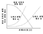
투석 센터의 모니터링 프로그램은 노동 부담 및 임상 워크플로우에 대한 영향을 감소시키기 위해 효율적이고 객관적이어야 한다. 신체 검사는 환자당 추가적인 시간을 필요로 하고 기술과 경험을 요구하는 주관적인 척도이기 때문에, 점점 더 사용되지 않는다. 신체 검사의 한 가지 중요한 양태는 청진인데, 여기서는 청진기를 사용하여 이상음(bruit)(혈관 협착 또는 다른 이상에 의해 야기되는 병리학적 혈류 사운드)을 검출한다. 이상음의 수학적 분석, 즉, 음파 혈관 조영도(phonoangiogram: PAG)는 이상음 스펙트럼 특성으로부터 협착 추정을 가능하게 하였다. 그러나, PAG에 대한 이전 작업은, 청진기를 사용하여 혈관 액세스의 한 개 또는 두 개의 위치로부터 이상음을 기록하는 것에 의해 제한되었다.Monitoring programs in dialysis centers should be efficient and objective to reduce labor burden and impact on clinical workflows. Physical examination is increasingly obsolete as it is a subjective measure that requires additional time per patient and requires skill and experience. One important aspect of physical examination is auscultation, in which a stethoscope is used to detect bruits (pathological blood flow sounds caused by stenosis of blood vessels or other abnormalities). Mathematical analysis of abnormal sounds, ie, phonoangiogram (PAG), made it possible to estimate stenosis from the abnormal sound spectral characteristics. However, previous work on PAGs has been limited by using a stethoscope to record abnormal sounds from one or two locations of vascular access.
다양한 양태에서, 혈관 시스템의 음향 신호를 검출하기 위한 장치가 본 명세서에서 설명된다. 장치는 적어도 하나의 음향 센서를 포함할 수 있다. 적어도 하나의 음향 센서는 관통하는 구멍을 획정하는 구조물을 포함할 수 있다. 압전 폴리머 층은 제1 면과 대향하는 제2 면을 가질 수 있다. 압전 폴리머 층은 구조물을 통해 연장되는 구멍을 가로질러 연장된다. 제1 전극은 폴리머 층의 제1 면 상에서 배치될 수 있다. 제2 전극은 폴리머 층의 제2 면 상에서 배치될 수 있다. 폴리머 결합층(polymer engagement layer)이 폴리머 층의 제1 면에 기대어 배치될 수 있고 구조물을 통해 연장되는 구멍 내에서 적어도 부분적으로 배치될 수 있다.In various aspects, an apparatus for detecting an acoustic signal of a vascular system is described herein. The device may include at least one acoustic sensor. The at least one acoustic sensor may include a structure defining an aperture therethrough. The piezoelectric polymer layer may have a second side opposite the first side. The piezoelectric polymer layer extends across the aperture extending through the structure. The first electrode may be disposed on the first side of the polymer layer. A second electrode may be disposed on the second side of the polymer layer. A polymer engagement layer may be disposed against the first side of the polymer layer and disposed at least partially within the aperture extending through the structure.
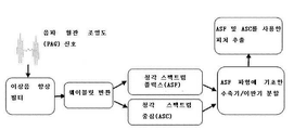
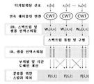
방법은 다음의 것을 포함할 수 있다: 이상음 향상 필터링 데이터(bruit enhanced filtered data)를 생성하기 위해 본 명세서에서 개시되는 바와 같은 장치를 사용하여 수집되는 데이터에 이상음 향상 필터(bruit enhancing filter)를 적용하는 것. 웨이블릿 데이터를 제공하기 위해 이상음 향상 필터링 데이터에 웨이블릿 변환이 적용될 수 있다.The method may include: applying a bruit enhancing filter to data collected using an apparatus as disclosed herein to generate bruit enhanced filtered data. to apply. A wavelet transform may be applied to the abnormal sound enhancement filtering data to provide wavelet data.
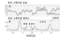
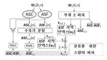
방법은, 웨이블릿 데이터로부터 청각 스펙트럼 플럭스 파형(auditory spectral flux waveform: ASF)을 생성하는 것 및 웨이블릿 데이터로부터 청각 스펙트럼 중심 파형(auditory spectral centroid waveform: ASC)을 생성하는 것을 더 포함할 수 있다.The method may further include generating an auditory spectral flux waveform (ASF) from the wavelet data and generating an auditory spectral centroid waveform (ASC) from the wavelet data.
방법은 청각 스펙트럼 플럭스 파형 및 청각 스펙트럼 중심 파형에 대해 수축기(systole)/이완기(diastole) 분할(segmentation)을 수행하는 것을 더 포함할 수 있다.The method may further include performing systole/diastole segmentation on the auditory spectral flux waveform and the auditory spectral center waveform.
청각 스펙트럼 플럭스 파형 및 청각 스펙트럼 중심 파형에 대해 수축기/이완기 분할을 수행하는 것은 다음의 것 중 적어도 하나를 계산하는 것을 포함할 수 있다: ASC의 수축기 세그먼트의 평균값, ASF의 수축기 세그먼트의 제곱 평균 제곱근(root mean square: RMS), ASC의 수축기 세그먼트의 평균값과 ASC의 이완기 세그먼트의 평균값 사이의 차이, 또는 ASC의 수축기 세그먼트의 평균과 ASF의 수축기 세그먼트의 RMS의 곱.Performing systolic/diastolic segmentation on the auditory spectral flux waveform and the auditory spectral center waveform may include calculating at least one of: the mean value of the systolic segment of the ASC, the root mean square of the systolic segment of the ASF ( root mean square: RMS), the difference between the mean of the systolic segment of ASC and the mean of the diastolic segment of ASC, or the product of the mean of the systolic segment of ASC and the RMS of the systolic segment of ASF.
방법은 다음의 것을 더 포함할 수 있다: 제1 센서로부터의 데이터에 대한 ASF의 임계치의 교차의 제1 시간을 결정하는 것; 혈류 방향과 관련하여 제1 센서에 대해 원위에 있는 제2 센서로부터의 데이터에 대한 ASF의 임계치의 교차의 제2 시간을 결정하는 것; 및 제1 시간과 제2 시간 사이의 차이를 계산하는 것.The method may further include: determining a first time of intersection of the threshold of the ASF for the data from the first sensor; determining a second time of intersection of the threshold of the ASF for data from a second sensor distal to the first sensor with respect to blood flow direction; and calculating a difference between the first time and the second time.
방법은 제1 시간과 제2 시간 사이의 차이에 기초하여 협착도(degree of stenosis)를 결정하는 것을 더 포함할 수 있다.The method can further include determining a degree of stenosis based on a difference between the first time and the second time.
다양한 양태에서, 방법은 협착도(degree of stenosis: DOS)를 결정하기 위해 ASC, ASF, 및 시간 데이터에 대해 회귀(regression)(예를 들면, 가우시안(Gaussian) 프로세스 회귀)를 수행하는 것을 포함할 수 있다. 적어도 하나의 범위(예를 들면, 경증(mild), 중등증(moderate) 및 중증(severe)) 내에서 DOS를 분류하기 위해 머신 러닝 분류기가 사용될 수 있다. 머신 러닝 분류기는 서포트 벡터 머신(support vector machine)을 포함할 수 있다.In various aspects, a method may include performing a regression (eg, a Gaussian process regression) on the ASC, ASF, and temporal data to determine a degree of stenosis (DOS). can A machine learning classifier may be used to classify DOS within at least one range (eg, mild, moderate and severe). A machine learning classifier may include a support vector machine.
시스템은 본 명세서에서 개시되는 바와 같은 장치 및 컴퓨팅 디바이스를 포함할 수 있다. 컴퓨팅 디바이스는 적어도 하나의 프로세서 및 적어도 하나의 프로세서와 통신하는 메모리를 포함할 수 있는데, 여기서 메모리는, 적어도 하나의 프로세서에 의해 실행될 때, 본 명세서에서 개시되는 바와 같은 방법을 수행하는 명령어를 포함한다.A system may include an apparatus and a computing device as disclosed herein. A computing device may include at least one processor and a memory in communication with the at least one processor, wherein the memory includes instructions that, when executed by the at least one processor, perform a method as disclosed herein. .
본 발명의 추가적인 이점은 후속하는 설명에서 부분적으로 기술될 것이며, 부분적으로는 설명으로부터 명백할 것이거나, 또는 본 발명의 실시에 의해 학습될 수도 있다. 본 발명의 이점은 첨부된 청구범위에서 특히 지적되는 요소 및 조합에 의해 실현되고 달성될 것이다. 전술한 일반적인 설명 및 다음의 상세한 설명 둘 모두는 예시적이고 설명적인 것에 불과하며, 청구되는 바와 같은 본 발명을 제한하지는 않는다는 것이 이해되어야 한다.Additional advantages of the invention will be set forth in part in the description that follows, and in part will be apparent from the description, or may be learned by practice of the invention. The advantages of the invention will be realized and attained by means of the elements and combinations particularly pointed out in the appended claims. It is to be understood that both the foregoing general description and the following detailed description are exemplary and explanatory only, and do not limit the invention as claimed.
본 발명의 바람직한 실시형태의 이들 및 다른 피처는, 첨부의 도면을 참조하는 상세한 설명에서 더욱 명백해질 것인데, 첨부의 도면에서:
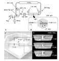
도 1은, 본 명세서에서 개시되는 실시형태에 따른, 임상 시스템 및 센서 어레이의 개략도를 예시한다.
도 2는 다양한 제조의 스테이지에서의 도 1에서와 같은 센서 어레이의 센서의 복수의 개략도를 예시한다.
도 3A는 본 명세서에서 개시되는 실시형태에 따른 센서 어레이의 상면도이다. 도 3B는 도 3A에서와 같은 센서 어레이의 일부의 측면 사시도이다. 도 3C는 어레이가 굴곡된 구성에 있는 도 3A에서와 같은 센서 어레이의 측면도이다. 도 3D는 도 3A에서와 같은 센서 어레이의 단면도이다. 도 3E는 도 3A에서와 같은 센서 어레이의 측면도이다.
도 4는 테스트 대상과 상호 작용하는 도 1의 센서 어레이의 개략도이다.
도 5는 본 명세서에서 개시되는 실시형태에 따른 센서 어레이를 포함하는 시스템의 개략도이다.
도 6은 본 명세서에서 개시되는 실시형태에 따른 센서 어레이를 포함하는 시스템의 다른 개략도이다.
도 7은 본 명세서에서 개시되는 실시형태에 따른 센서 어레이를 포함하는 시스템의 또 다른 개략도이다.
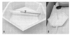
도 8A는 도 1의 센서 어레이를 테스트하기 위한 테스트 장치의 개략도이다. 도 8B는 도 1의 센서 어레이의 센서 사이의 크로스토크(cross-talk)를 측정하기 위한 테스트 장치의 개략도를 예시한다.
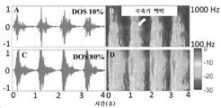
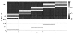
도 9A 및 도 9B는, 각각, 낮은(10%) 협착도(DOS)를 갖는 혈관 액세스 모형(vascular access phantom)에 대해 기록되는 PAG 및 스펙트로그램(spectrogram)을 예시한다. 도 9C 및 도 9D는, 각각, 높은(80%) DOS를 갖는 혈관 액세스 모형에 대해 기록되는 PAG 및 스펙트로그램을 예시한다.
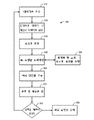
도 10은 PAG 신호를 프로세싱하고 관련 피처를 추출하기 위한 방법을 예시한다.
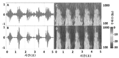
도 11A 및 도 11C는, 각각, 이상음 향상 필터 이전의 PAG 신호 및 이의 스펙트로그램을 예시한다. 도 11B 및 도 11D는, 각각, 이상음 향상 필터 이후의 PAG 신호 및 그것의 스펙트로그램을 예시한다.
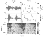
도 12A는 프로세싱되지 않은 PAG 신호의 플롯을 도시한다. 도 12B는 이상음 향상 필터 이후의 도 12A의 데이터를 예시한다. 도 12C는 음향 데이터의 연속 웨이블릿 변환(continuous wavelet transform: CWT)을 예시한다. 도 12D는 분할된 피처 추출을 위해 파형을 세그먼트로 분할하기 위한 사용을 위해 스펙트럼 1차 도함수를 근사하는 청각 스펙트럼 플럭스(Auditory Spectral Flux: ASF)를 예시한다. 도 12E는 청각 스펙트럼 중심(Auditory Spectral Centroid: ASC)을 예시한다.
도 13A는 도 1에서와 같은 센서 어레이를 테스트하기 위한 테스트 시스템이다. 도 13B는 도 13A에서와 같은 테스트 시스템 상에 배치되는 어레이의 개략적인 다이어그램이다. 도 13C는 모형 테스트 장치의 이미지이다. 도 13D는 도 13C에서와 같은 모형 테스트 장치를 따라 상이한 단면적을 보여주는 복수의 도면이다.
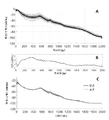
도 14A는 인간 환자에 대한 PAG 스펙트럼을 예시한다. 도 14B는 각각의 주파수에 대한 사분위수간 범위(inter-quartile range)를 예시한다. 도 14C는 튜닝된 혈관 모형 파워 스펙트럼과 평균 인간 스펙트럼 사이의 비교를 예시한다.
도 15는 모형과 예시적인 센서 어레이를 포함하는 테스트 장비(test rig)를 예시한다.
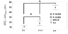
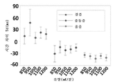
도 16은 경증(DOS < 40%), 중등증(40% < DOS < 60%) 및 중증(DOS < 60%)에 대한 ![]()
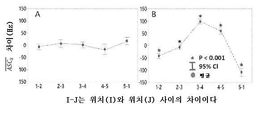
도 17은 모형 상의 인접한 위치 사이의 ![]()
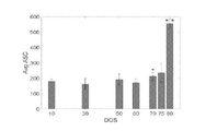
도 18은 ![]()
도 19는 특성 묘사 테스트에 따른 테스트 보드를 예시한다.
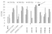
도 20A 내지 도 20E는 상이한 지지체 층(backing layer)을 갖는 센서에 대한 주파수 응답을 예시한다.
도 21은 다수의 주파수에서의 지지체와 상이한 사이즈를 갖는 센서 사이의 신호 비교를 예시한다.
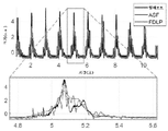
도 22는 Hilbert(힐베르트) 엔벨로프, 청각 스펙트럼 플럭스, 및 주파수 도메인 선형 예측 모델링(frequency domain linear prediction-modeled: FDLP 모델링) 엔벨로프를 포함할 수 있는 PAG로부터 획득되는 분석 신호를 예시한다.
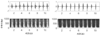
도 23은, 둘 모두 FDLP 수축기 펄스 향상을 사용하는, (A) 종래의 청진기, 및 (B) 실리콘 겔을 갖는 2㎜ 센서로부터 기록되는 PAG의 시간 및 웨이블릿 스케일 표현을 예시한다.
도 24A 및 도 24B는 실리콘 튜빙(silicone tubing) 주위에서 봉합 밴드를 사용하고 생체 모방 실리콘 고무 몰드로 주조되는 혈관 협착 모형의 제조에서의 단계를 예시한다.
도 25A 및 도 25B는, 각각, 통상적인 투석 환자 및 협착이 없는 혈관 모형의 음파 혈관 조영도 및 웨이블릿 변환을 예시한다.
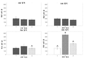
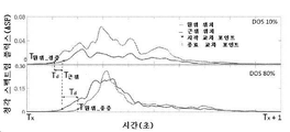
도 26은 10%와 80% 사이의 DOS를 갖는 모형에 대한 다양한 흐름 타입 및 기록 위치에서의 ASC 값을 도시하는 플롯을 예시한다.
도 27은 10%와 80% 사이의 DOS를 갖는 모형에 대한 모두 세 개의 기록 위치에서의 생리학적 흐름 레벨에 걸친 평균 ASC 값을 도시하는 플롯이다.
도 28은 각각의 모형에 대해 위치 2에서 기록되는 모든 흐름 타입에 대한 평균 ASC 값을 도시하는 플롯이다.
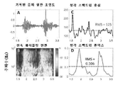
도 29A는 시간 도메인 혈액 사운드를 도시하는 플롯이다. 도 29B는, 본 명세서에서 개시되는 바와 같은 센서 어레이를 사용하여, 본 명세서에서 개시되는 바와 같은 모형으로부터 수집되는 CWT 스펙트럼 도메인을 도시하는 플롯이다. 도 29C는 추출된 분석 신호 청각 스펙트럼 플럭스를 도시하는 플롯이다. 도 29D는 임계치 설정(thresholding)에 의해 계산되는 수축기 시작/종료 시간을 도시하는 플롯이다.
도 30A는 다수의 임계 포인트를 통해 ASF 개시 검출을 도시하는 플롯이다. 도 30B는 ASF RMS 값의 25% 포화도를 갖는 Td의 성능을 도시하는 플롯이다. 도 30C는 5%, 25% 및 50%의 임계 값을 도시하는 플롯이다.
도 31은 근위 및 원위 위치에서 계산되는 ASF가 Td에서 역전을 나타내는 것을 도시하는 플롯이다.
도 32는 유량의 범위에 대한 Td 및 DOS 등급을 도시하는 플롯이다.
도 33은 각각의 DOS 등급에 대한 시간 차이를 도시하는 플롯이다.
도 34는 각각의 DOS 등급에 대한 평균 속도 변화를 도시하는 플롯이다.
도 35는, 본 명세서에서 개시되는 실시형태에 따른, 컴퓨팅 디바이스를 포함하는 시스템의 개략도이다.
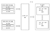
도 36은, 분류를 위한 피처를 추출하기 위해 아날로그 대 디지털 변환 및 디지테이션(digitation) 이후의 디지털 신호 프로세싱에서 신호 대 노이즈 비율을 최대화하고 앨리어싱을 방지하기 위한 아날로그 도메인에서의 신호 프로세싱을 예시하는 개략적인 다이어그램이다.
도 37은 부위 특이적 신호 대역폭(site-specific signal bandwidth)을 나타내기 위해 75% 협착을 기준으로 상이한 위치에서 기록되는 파워 스펙트럼 밀도를 도시하는 플롯이다. 일반적으로, 협착 이후의 부위는, 난류 혈류(turbulent blood flow)의 국소적 존재 때문에, 더 넓은 신호 대역폭을 갖는다.
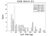
도 38은, 기록 부위에 기초하여 집성된 DOS 10 내지 90%에 대한 156개의 PAG 기록에 대한 95% 파워 대역폭을 도시하는 막대 그래프이다. 부위 2 및 3에서의 기록은 협착도 또는 유량과 무관하게 더 넓은 대역폭을 나타낸다. 이것은 분류기 방법론의 기초를 형성하는데, 협착이 존재하는 상태에서 상승된 파워와 주파수 성분(frequency content) 사이에는 뚜렷한 상관 관계가 있기 때문이다.
도 39는, 아날로그 신호 프로세싱 섹션에서 신호 다이나믹스(signal dynamics)를 정확하게 캡처하기 위해 적어도 1,600㎐의 필수 대역폭을 나타낸 DOS 10-90%를 사용하여 기록되는 PAG에 대한 사분위수 범위 분석을 도시주는 차트를 예시한다. 안전 계수(safety factor)를 포함하여, 인터페이스 증폭기는 노이즈를 제한하기 위해 2.25㎑ 대역폭에 맞게 설계되었다.
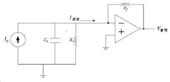
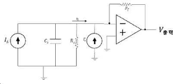
도 40은 100㎐에서의 측정된 임피던스에 기초하여 출력 전류(I신호)와 병렬인 저항기(Rs) 및 커패시터(Cs)로서 간단하게 모델링되는 폴리비닐리덴-플루오라이드(PVDF) 트랜스듀서의 개략적인 다이어그램이다.
도 41은 연산 증폭기 개루프 전달 함수 및 노이즈 전달 함수 대 주파수의 예시적인 플롯이다. 이상적으로, 노이즈 전달 함수는 연산 증폭기 이득이 감쇠되기 시작할 때까지 더 편평해질 것이다(예를 들면, "B").
도 42는, 입력 노이즈 소스로서 기능하는 병렬 전류 소스인 ![]()
도 43은 100 내지 1500㎐로부터의 6개의 단일 톤 주파수를 갖는 인위적으로 생성된 테스트 파형의 스펙트로그램을 도시하는 플롯이다. ASF 곡선(하위)은, 스펙트럼 1차 도함수를 근사하는, 모든 주파수 변경에서의 스파이크를 도시한다.
도 44는 100 내지 1500㎐로부터의 6개의 단일 톤 주파수를 갖는 인위적으로 생성된 테스트 파형의 스펙트로그램을 도시하는 플롯이다. ASC 곡선은 각각의 시점에서의 사인파의 주파수를 설명한다.
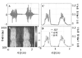
도 45는 시간 도메인 이상음(A) 및 연속 웨이블릿 변환 스펙트럼 도메인(B)이다. 설명 신호(설명 신호) 청각 스펙트럼 중심 및 플럭스는 CWT 계수(C,D)로부터 추출되었다. 설명 신호의 RMS 값은 시간 도메인 파형으로부터 유도되는 스칼라 피처의 일례이다.
도 46은, 협착도에 따라 그러나 또한 수축기 단계와 이완기 단계 사이에서 변하는 청각 스펙트럼 중심(ASC)의 플롯(A) 및 ASC의 RMS 값(ASCRMS)이 별개로 계산될 수 있도록 박동 단계(pulsatile phase) 사이의 분할을 가능하게 하는 청각 스펙트럼 플럭스(ASF) 파형의 플롯이다.
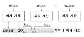
도 47은 각각의 기록 부위로부터 피처가 유도될 수 있는 방법 및 분류를 위해 피처 세트로 결합될 수 있는 방법을 예시하는 다이어그램이다.
도 48은 Td의 역전을 나타낸 근위 및 원위 위치에서 계산되는 ASF의 플롯을 예시한다. 중등증 및 중증 DOS에서, Td는 음수가 되었는데, 흐름 속도가 증가한다는 것을 나타낸다.
도 49는 데이터 프로세싱을 도시하는 다이어그램을 예시한다. 피처가 추출됨에 따라, 데이터세트의 차원은 감소되어 피처의 최종 세트를 산출한다. 각각의 부위가 부위 고유의 피처와 부위 내 피처 차이로부터 추출되는 피처를 가지기 때문에, F[S,M]의 전체 피처 세트는 M 부위에 대한 S 피처를 가지고 생성된다.
도 50은 인접한 부위 사이의 피처 차이로부터 유도되는 공간적 피처를 사용한 협착 위치 파악을 예시하는 예시적인 다이어그램이다. 이 예에서, 부위 사이의 ![]()
도 51은 센서 위치 사이의 ASCS에서의 차이를 도시하는 플롯을 예시한다. 예시되는 바와 같이, 인접한 위치 사이의 ASCS에서의 차이는 0% DOS(p > 0.05)(A)에 대해 유의미한 변화를 나타내지 않았다. 협착(위치 2에서의 협착 중심)에 대해 원위에 있는 위치에서는 큰 스펙트럼 시프트(B). 데이터는 모든 위치에 대해 30% < DOS < 90%, p < 0.001를 갖는 모형에 대해 플롯되었다. 분산의 분석 및 Tukey(터키)의 테스트는 유의도 레벨 α = 0.05에서 ASC 평균에서 통계적으로 유의미한 차이를 식별하였다.
도 52는, ![]()
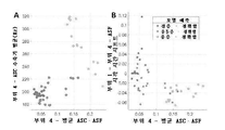
도 53A는 ASC 수축기 평균 대 평균 ASC - ASF의 플롯을 예시한다. 도 53B는 ASC 시작 시간 대 평균 ASC - ASF의 플롯을 예시한다. 2차(quadratic) SVM은 100% 정확도를 가지고 DOS를 경증(< 30%), 중등증(30% < DOS < 60%) 및 중증(DOS > 60%)으로서 분류하였다. 이것은, 포함된 피처가 피처 공간(A,B)에서 선형적으로 완전히 분리되지 않기 때문에, SVM의 이점을 설명한다.
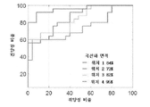
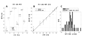
도 54A는 각각의 시험관 내 혈관 협착 모형에 대한 지수 가우시안 프로세스 회귀 추정 협착도(exponential Gaussian process regression estimated degree of stenosis)이다. 도 54B는 4.3%의 RMS 오차를 갖는 트레이닝된 모델 추정 협착도를 도시하는 플롯이다. 도 54C는 모든 테스트된 협착에 대해 그리고 50%를 초과하는 협착에 대해, 각각, [-11% 14%] 및 [-11% 3%]의 오차 범위를 도시하는 플롯이다.
도 55는, 본 명세서에서 개시되는 바와 같은, 인공 지능(artificial intelligence: AI)을 트레이닝시키기 위한 예시적인 시스템이다.
도 56은 협착도를 결정하기 위해 AI를 사용하기 위한 예시적인 방법이다.BRIEF DESCRIPTION OF THE DRAWINGS These and other features of preferred embodiments of the present invention will become more apparent from the detailed description with reference to the accompanying drawings, in which:
1 illustrates a schematic diagram of a clinical system and a sensor array, in accordance with embodiments disclosed herein.
2 illustrates a plurality of schematic views of a sensor of a sensor array as in FIG. 1 at various stages of manufacture;
3A is a top view of a sensor array according to an embodiment disclosed herein. 3B is a side perspective view of a portion of a sensor array as in FIG. 3A; 3C is a side view of the sensor array as in FIG. 3A with the array in a curved configuration; Fig. 3D is a cross-sectional view of the sensor array as in Fig. 3A; Fig. 3E is a side view of the sensor array as in Fig. 3A;
Fig. 4 is a schematic diagram of the sensor array of Fig. 1 interacting with a test subject;
5 is a schematic diagram of a system including a sensor array in accordance with embodiments disclosed herein;
6 is another schematic diagram of a system including a sensor array in accordance with embodiments disclosed herein.
7 is another schematic diagram of a system including a sensor array according to an embodiment disclosed herein.
Fig. 8A is a schematic diagram of a test apparatus for testing the sensor array of Fig. 1; FIG. 8B illustrates a schematic diagram of a test apparatus for measuring cross-talk between the sensors of the sensor array of FIG. 1 ;
9A and 9B illustrate, respectively, PAG and spectrograms recorded for a vascular access phantom with low (10%) stenosis (DOS). 9C and 9D illustrate the PAG and spectrograms recorded for a vascular access model with high (80%) DOS, respectively.
10 illustrates a method for processing a PAG signal and extracting relevant features.
11A and 11C illustrate, respectively, a PAG signal before an abnormal sound enhancement filter and a spectrogram thereof. 11B and 11D illustrate the PAG signal and its spectrogram after the abnormal sound enhancement filter, respectively.
12A shows a plot of the unprocessed PAG signal. 12B illustrates the data of FIG. 12A after the abnormal sound enhancement filter. 12C illustrates a continuous wavelet transform (CWT) of acoustic data. 12D illustrates Auditory Spectral Flux (ASF) approximating spectral first derivative for use to segment a waveform into segments for segmented feature extraction. 12E illustrates the Auditory Spectral Centroid (ASC).
13A is a test system for testing the sensor array as in FIG. 1 . 13B is a schematic diagram of an array disposed on a test system as in FIG. 13A. 13C is an image of the mock test apparatus. Fig. 13D is a plurality of views showing different cross-sectional areas along the mock test apparatus as in Fig. 13C.
14A illustrates the PAG spectrum for a human patient. 14B illustrates the inter-quartile range for each frequency. 14C illustrates a comparison between the tuned vessel model power spectrum and the mean human spectrum.
15 illustrates a test rig including a mockup and an exemplary sensor array.
16 is a graph for mild (DOS < 40%), moderate (40% < DOS < 60%) and severe (DOS < 60%) cases.![]()
17 is a diagram between adjacent positions on the model.![]()
18 is![]()
19 illustrates a test board according to a characterization test.
20A-20E illustrate the frequency response for sensors with different backing layers.
21 illustrates a signal comparison between a support and a sensor having a different size at multiple frequencies.
22 illustrates an analysis signal obtained from a PAG that may include a Hilbert envelope, an auditory spectral flux, and a frequency domain linear prediction-modeled (FDLP modeling) envelope.
23 illustrates a temporal and wavelet scale representation of a PAG recorded from a 2 mm sensor with (A) a conventional stethoscope, and (B) a silicone gel, both using FDLP systolic pulse enhancement.
24A and 24B illustrate the steps in the fabrication of a vascular stenosis model that is cast into a biomimetic silicone rubber mold using a suture band around silicone tubing.
25A and 25B illustrate sonic angiograms and wavelet transformations of a typical dialysis patient and a vascular model without stenosis, respectively.
26 illustrates a plot showing ASC values at various flow types and recording locations for models with DOS between 10% and 80%.
27 is a plot showing mean ASC values across physiological flow levels at all three recording locations for models with DOS between 10% and 80%.
28 is a plot showing the average ASC values for all flow types recorded at
29A is a plot depicting the time domain blood sound. 29B is a plot showing the CWT spectral domain collected from a model as disclosed herein, using a sensor array as disclosed herein. 29C is a plot showing the extracted analyte signal auditory spectral flux. 29D is a plot showing systolic start/end times calculated by thresholding.
30A is a plot showing ASF onset detection through multiple threshold points. 30B is a plot showing the performance of Td with 25% saturation of ASF RMS values. 30C is a plot showing the threshold values of 5%, 25% and 50%.
FIG. 31 is a plot showing that ASF calculated at proximal and distal positions exhibits reversal at T d .
32 is a plot showing T d and DOS ratings for a range of flow rates.
33 is a plot showing the time difference for each DOS class.
34 is a plot showing the average speed change for each DOS class.
35 is a schematic diagram of a system including a computing device, in accordance with embodiments disclosed herein.
36 is a schematic diagram illustrating signal processing in the analog domain to maximize signal-to-noise ratio and avoid aliasing in analog-to-digital conversion and digital signal processing after digitation to extract features for classification is a diagram.
37 is a plot showing the power spectral densities recorded at different locations relative to a 75% constriction to indicate site-specific signal bandwidth. In general, the site after stenosis has a wider signal bandwidth due to the local presence of turbulent blood flow.
38 is a bar graph showing 95% power bandwidth for 156 PAG writes for DOS 10-90% aggregated based on write site. Recordings at
39 is a chart showing interquartile range analysis for a PAG recorded using DOS 10-90% showing the required bandwidth of at least 1,600 Hz to accurately capture signal dynamics in the analog signal processing section; exemplify Including the safety factor, the interface amplifier is designed for a 2.25kHz bandwidth to limit noise.
40 is a polyvinylidene-fluoride (PVDF) transducer modeled simply as a resistor (R s ) and a capacitor (C s ) in parallel with the output current (I signal ) based on the measured impedance at 100 Hz. This is a schematic diagram.
41 is an exemplary plot of an op amp open loop transfer function and noise transfer function versus frequency. Ideally, the noise transfer function will be flatter until the op amp gain begins to decay (eg, “B”).
42 is a parallel current source serving as an input noise source;![]()
43 is a plot showing a spectrogram of an artificially generated test waveform with six single tone frequencies from 100 to 1500 Hz. The ASF curve (bottom) shows the spike at every frequency change, approximating the spectral first derivative.
44 is a plot showing a spectrogram of an artificially generated test waveform with six single tone frequencies from 100 to 1500 Hz. The ASC curve describes the frequency of the sine wave at each time point.
45 is a time domain anomaly (A) and a continuous wavelet transform spectral domain (B). The explanatory signal (explanatory signal) auditory spectral center and flux were extracted from the CWT coefficients (C,D). The RMS value of the explanatory signal is an example of a scalar feature derived from a time domain waveform.
Figure 46 is a plot (A) of the auditory spectral center (ASC) that varies with the degree of constriction but also between the systolic and diastolic phases (A) and the pulsatile phase so that the RMS values of the ASC (ASC RMS ) can be calculated separately. ) is a plot of the auditory spectral flux (ASF) waveform that allows for division between
47 is a diagram illustrating how features can be derived from each recording site and how they can be combined into a set of features for classification.
48 illustrates a plot of ASF calculated at proximal and distal positions showing reversal of T d . At moderate and severe DOS, T d became negative, indicating an increase in flow rate.
49 illustrates a diagram illustrating data processing. As features are extracted, the dimensions of the dataset are reduced to yield the final set of features. Since each site has its own site-specific features and features extracted from feature differences within the site, a full set of features of F[S,M] is created with S features for M sites.
50 is an exemplary diagram illustrating stenosis localization using spatial features derived from feature differences between adjacent regions. In this example, between the sites![]()
51 illustrates a plot depicting the difference in ASC S between sensor positions. As illustrated, the difference in ASC S between adjacent positions did not show a significant change for 0% DOS (p > 0.05) (A). Large spectral shift at positions distal to the stenosis (center of stenosis at position 2) (B). Data were plotted for models with 30% < DOS < 90%, p < 0.001 for all locations. Analysis of variance and Tukey's (Turkey) test identified statistically significant differences in ASC means at the significance level α = 0.05.
52 is![]()
53A illustrates a plot of ASC systolic mean versus mean ASC - ASF. 53B illustrates a plot of ASC onset time versus mean ASC - ASF. The quadratic SVM classified DOS as mild (<30%), moderate (30%<DOS<60%) and severe (DOS>60%) with 100% accuracy. This explains the advantage of SVM, since the included features are not completely linearly separated in feature space (A,B).
54A is an exponential Gaussian process regression estimated degree of stenosis for each in vitro vascular stenosis model. 54B is a plot showing the trained model estimate narrowness with an RMS error of 4.3%. 54C is a plot showing the error ranges of [-11% 14%] and [-11% 3%], respectively, for all tested stenosis and for stenosis greater than 50%.
55 is an example system for training artificial intelligence (AI), as disclosed herein.
56 is an exemplary method for using AI to determine stenosis.
이제, 본 발명은 본 발명의 모든 실시형태가 아닌 몇몇 실시형태가 도시되는 첨부의 도면을 참조하여 이하에서 더욱 완전하게 설명될 것이다. 실제로, 본 발명은 많은 상이한 형태로 구현될 수도 있고 본 명세서에서 기술되는 실시형태로 제한되는 것으로 해석되어서는 안된다; 오히려, 이들 실시형태는 본 개시내용이 적용 가능한 법적 요건을 충족하도록 제공된다. 같은 숫자는 전체에 걸쳐 같은 요소를 가리킨다. 본 발명은 설명되는 특정한 방법론 및 프로토콜로 제한되지 않으며, 그러한 만큼 다양할 수도 있다는 것이 이해되어야 한다. 본 명세서에서 사용되는 전문 용어는 단지 특정한 실시형태를 설명하는 목적을 위한 것이며, 본 발명의 범위를 제한하도록 의도되지는 않는다는 것이 또한 이해되어야 한다.DETAILED DESCRIPTION OF THE PREFERRED EMBODIMENTS The present invention will now be more fully described below with reference to the accompanying drawings in which some but not all embodiments of the invention are shown. Indeed, the present invention may be embodied in many different forms and should not be construed as limited to the embodiments set forth herein; Rather, these embodiments are provided so that this disclosure will satisfy applicable legal requirements. Like numbers refer to the same elements throughout. It is to be understood that the present invention is not limited to the particular methodologies and protocols described, as it may vary as much. It should also be understood that the terminology used herein is for the purpose of describing particular embodiments only, and is not intended to limit the scope of the present invention.
전술한 설명 및 관련된 도면에 제시되는 교시의 이점을 갖는 본 발명이 속하는 기술 분야의 숙련자는, 본 명세서에서 기술되는 본 발명의 많은 수정예 및 다른 실시형태를 떠올릴 것이다. 따라서, 본 발명은 개시되는 특정한 실시형태로 제한되지 않는 다는 것 및 수정예 및 다른 실시형태가 첨부된 청구범위의 범위 내에 포함되도록 의도된다는 것이 이해되어야 한다. 본 명세서에서는 특정한 용어가 활용되지만, 그들은 일반적이고 설명적인 의미로서만 사용되며, 제한의 목적을 위해서는 사용되지는 않는다.Many modifications and other embodiments of the invention described herein will occur to those skilled in the art, having the benefit of the teachings presented in the foregoing description and associated drawings, to which this invention pertains. Accordingly, it is to be understood that the present invention is not limited to the specific embodiments disclosed and that modifications and other embodiments are intended to be included within the scope of the appended claims. Although specific terminology is employed herein, they are used in a generic and descriptive sense only and not for purposes of limitation.
본 명세서에서 사용되는 바와 같이, 단수 형태는 문맥 상 명백하게 다르게 지시하지 않는 한 복수 지시 대상을 포함한다. 예를 들면, 용어 "음향 센서"의 사용은 그러한 음향 센서 등 중 하나 이상을 지칭할 수 있다.As used herein, singular forms include plural referents unless the context clearly dictates otherwise. For example, use of the term “acoustic sensor” may refer to one or more of such acoustic sensors and the like.
본 명세서에서 사용되는 모든 기술적 및 과학적 용어는, 달리 명확하게 나타내어지지 않는 한, 본 발명이 속하는 기술 분야에서 통상의 지식을 가진 자에게 일반적으로 이해되는 것과 동일한 의미를 갖는다.All technical and scientific terms used herein have the same meaning as commonly understood by one of ordinary skill in the art to which this invention belongs, unless clearly indicated otherwise.
본 명세서에서 사용될 때, 용어 "옵션 사항의(optional)" 또는 "옵션 사항으로(optionally)"는, 후속하여 설명되는 이벤트 또는 상황이 발생할 수도 있거나 또는 발생하지 않을 수도 있다는 것 및 그 설명은 상기 이벤트 또는 상황이 발생하는 인스턴스 및 이것이 발생하지 않는 인스턴스를 포함한다는 것을 의미한다.As used herein, the term “optional” or “optionally” means that the subsequently described event or circumstance may or may not occur and that description refers to that event. or that the situation includes instances where it occurs and instances where it does not.
본 명세서에서 사용되는 바와 같이, 용어 "중 적어도 하나"는 "중 하나 이상"과 동의어인 것으로 의도된다. 예를 들면, "A, B 및 C 중 적어도 하나"는 A만을, B만을, C만을, 각각의 조합을 명시적으로 포함한다.As used herein, the term “at least one of” is intended to be synonymous with “at least one of”. For example, “at least one of A, B and C” explicitly includes A only, B only, C only, and combinations of each.
범위는 "약" 하나의 특정한 값으로부터, 및/또는 "약" 다른 특정한 값까지로서 본 명세서에서 표현될 수 있다. 그러한 범위가 표현될 때, 다른 양태는 하나의 특정한 값으로부터 및/또는 다른 특정한 값까지를 포함한다. 유사하게, 값이, 선행사 "약"의 사용에 의해, 근사치로서 표현되는 경우, 특정한 값은 다른 양태를 형성한다는 것이 이해될 것이다. 범위 각각의 엔드포인트는, 다른 엔드포인트와 관련하여, 뿐만 아니라, 다른 엔드포인트와는 독립적으로 중요하다는 것이 추가로 이해될 것이다. 옵션 사항으로, 몇몇 양태에서, 값이 선행사 "약"의 사용에 의해 근사되는 경우, 특별히 언급된 값의 (위로 또는 아래로) 최대 15%, 최대 10%, 최대 5%, 또는 최대 1% 이내의 값이 그들 양태의 범위 내에 포함될 수 있다는 것이 고려된다. 유사하게, 선행사 "일반적으로"의 사용(예를 들면, "일반적으로 원형인")은, 최대 15%, 최대 10%, 최대 5%, 또는 최대 1%의 분산을 나타낼 수 있다.Ranges may be expressed herein as from "about" one particular value, and/or to "about" another particular value. When such a range is expressed, another aspect includes from the one particular value and/or to the other particular value. Similarly, when values are expressed as approximations, by use of the antecedent "about," it will be understood that the particular value forms another aspect. It will be further understood that each endpoint of the scope is significant, with respect to the other endpoints, as well as independently of the other endpoints. Optionally, in some embodiments, when a value is approximated by use of the antecedent "about," within at most 15%, at most 10%, at most 5%, or at most 1% (up or down) of the specifically stated value. It is contemplated that values of may be included within the scope of those embodiments. Similarly, use of the antecedent "generally" (eg, "generally circular") can indicate a variance of at most 15%, at most 10%, at most 5%, or at most 1%.
단어 "또는"은, 본 명세서에서 사용되는 바와 같이, 특정한 목록의 임의의 하나의 멤버를 의미하고 또한 그 목록의 멤버의 임의의 조합을 포함한다.The word “or,” as used herein, means any one member of a particular list and includes any combination of members of that list.
달리 명시적으로 언급되지 않는 한, 본 명세서에서 기술되는 임의의 방법은 그 단계가 특정한 순서로 수행되어야 하는 것을 규정하는 것으로 해석되어야 한다는 것이 어떤 식으로든 의도되지 않는다는 것이 이해되어야 한다. 따라서, 방법 청구항이 그 단계가 따라야 할 순서를 실제로 언급하지 않거나 또는 단계가 특정한 순서로 제한되어야 한다는 것이 청구항 또는 설명에서 달리 구체적으로 언급되지 않은 경우, 임의의 관점에서 순서가 추론되어야 한다는 것이 어떤 식으로든 의도되지 않는다. 이것은, 다음의 것을 비롯하여, 해석을 위한 임의의 가능한 비명시적 근거에 적용된다: 단계 또는 동작 흐름의 배열과 관련한 로직의 문제; 문법적 구성 또는 구두점으로부터 유도되는 평범한 의미; 및 명세서에서 설명되는 양태의 개수 또는 타입.It is to be understood that, unless explicitly stated otherwise, it is not intended in any way that any method described herein should be construed as stipulating that the steps are to be performed in a particular order. Thus, unless a method claim actually recites the order that the steps are to be followed, or unless the claim or description specifically states otherwise in the claim or description that the steps should be limited to a particular order, there is no indication that the order should be inferred in any respect. It is not intended to be This applies to any possible non-explicit basis for interpretation, including: problems of logic with respect to the arrangement of steps or flow of operations; plain meaning derived from grammatical construction or punctuation; and the number or type of aspects described in the specification.
다음의 설명은 완전한 이해를 제공하기 위해 특정한 세부 사항을 제공한다. 그럼에도 불구하고, 숙련된 기술자는 장치, 시스템, 및 장치를 사용하는 관련된 방법이 이들 특정한 세부 사항을 활용하지 않고도 구현되고 사용될 수 있다는 것을 이해할 것이다. 실제로, 장치, 시스템, 및 관련된 방법은, 예시된 장치, 시스템, 및 관련된 방법을 수정하는 것에 의해 실시될 수 있으며, 업계에서 종래에 사용되는 임의의 다른 장치 및 기술과 연계하여 사용될 수 있다.The following description provides specific details in order to provide a thorough understanding. Nevertheless, it will be understood by those skilled in the art that the apparatus, systems, and related methods of using the apparatus may be implemented and used without utilizing these specific details. Indeed, the apparatus, systems, and related methods may be practiced by modifying the illustrated apparatus, systems, and related methods, and may be used in connection with any other apparatus and technique conventionally used in the art.
본 명세서에서 추가로 개시되는 바와 같이, 현장 진료(point of care)에서 또는 환자의 집에서 예비 모니터링(prospective monitoring)을 가능하게 하기 위해, 대규모 마이크 어레이가 혈관 액세스 협착의 실시간 정량화를 위한 데이터 기록 및 디지털 신호 프로세싱 회로부(circuitry)와 결합될 수 있다. 음파 혈관 조영도(PAG)는 신체 검사의 확립된 요소를 구현할 수 있고, 피부 표면으로부터 측정하기 쉽고, 특히 혈관 액세스 구조물에 의해 생성된다.As further disclosed herein, to enable prospective monitoring at the point of care or at the patient's home, a large array of microphones can be used to record data for real-time quantification of vascular access stenosis and It may be coupled with digital signal processing circuitry. Acoustic angiograms (PAGs) can embody an established element of the physical examination, are easy to measure from the skin surface, and are particularly generated by vascular access structures.
이상음 스펙트럼 분석은 액세스 포인트에서 혈류의 수축기 및 이완기 성분을 분리할 수 있다. 청진기를 사용하는 것과 비교하여, 마이크 어레이는 혈관 이상을 정확하게 위치 지정하는 데 상당한 이점을 갖는다. 게다가, 박막 접촉 마이크는 종래의 청진기보다 더 큰 감도 및 대역폭을 갖는다. 예비 모니터링 시나리오에서, 마이크 어레이는, 길고 구불구불한 혈관 액세스를 따라 다수의 부위로부터 동시에 기록하기 위해 사용될 수 있다. 이상음 스펙트럼에서 부위별 차이(site-to-site difference)를 검출하고 주변 노이즈를 제거하기 위해, 채널 사이의 상관된 신호 프로세싱이 사용될 수 있다. 그 다음, 후속하는 이미징을 위해 위험에 처한 환자를 자동적으로 검출하기, 분류기 알고리즘 또는 다른 정량화 기술이 사용될 수 있다.Abnormal sound spectrum analysis can separate systolic and diastolic components of blood flow at the access point. Compared to using a stethoscope, microphone arrays have significant advantages in accurately locating vascular abnormalities. In addition, thin-film contact microphones have greater sensitivity and bandwidth than conventional stethoscopes. In a preliminary monitoring scenario, a microphone array can be used to simultaneously record from multiple sites along a long, tortuous vascular access. To detect site-to-site differences in the anomaly spectrum and to remove ambient noise, correlated signal processing between channels may be used. A classifier algorithm or other quantification technique may then be used to automatically detect patients at risk for subsequent imaging.
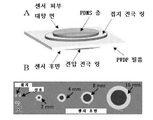
다양한 양태에서 그리고 도 1 내지 도 4를 참조하여, 하나 이상의 센서(102)를 포함하는 음향 센서 어레이(100)가 본 명세서에서 개시된다. 옵션 사항으로, 센서는 제1 축(104)을 따라 배열될 수 있다. 일부 옵션 사항의 양태에서, 센서(102)는 특정한 정맥의 경로를 추적하기 위해 비선형 배열로 배열될 수 있다. 또 다른 실시형태에서, 센서는 제1 축(104) 및 제1 축(104)에 수직인 제2 축(105)을 갖는 이차원 그리드로 배열될 수 있다. 각각의 센서(102)는 제1 전극(106) 및 제2 전극(108)을 포함할 수 있다. 옵션 사항으로, 제1 전극(106) 및 제2 전극(108) 각각은 그들을 관통하는 각각의 구멍(110)을 획정하는 환형 전극일 수 있다. 각각의 센서의 각각의 제1 및 제2 전극(106, 108)의 구멍(110)은 축 방향으로 정렬될 수 있다. 옵션 사항으로, 구멍(110)은 직경이 1 내지 3 밀리미터 사이에 있을 수 있거나, 또는 직경이 약 2밀리미터일 수 있다.In various aspects and with reference to FIGS. 1-4 , an
압전층(112)이 각각의 센서(102)의 제1 전극(106)과 제2 전극(108) 사이에서 배치될 수 있고 제1 전극(106) 및 제2 전극(108)의 구멍(110)에 걸쳐 있을 수 있다. 또 다른 옵션 사항의 양태에 따르면, 예를 들면, 가요성 인쇄 회로 보드와 같은 다른 구조물이 자신을 관통하는 구멍을 획정할 수 있고, 압전층(112)은 구조물 내의 상기 구멍을 가로질러 연장될 수 있다. 옵션 사항으로, 압전층(112)은 폴리머를 포함할 수 있다. 또 다른 양태에서, 예를 들면, 나일론(예를 들면, 나일론-11)의 혼합된 결정 형태, 티탄산 지르콘산 납 또는 티탄산 비스무트 나트륨과 같은 압전 세라믹 재료, 또는, 예를 들면, 비정질 플루오로폴리머 기판에 기초한 하전된 일렉트릿 필름(charged electret film)과 같은 다른 압전 트랜스듀서 재료가 사용될 수 있다.A
압전층(112)은 제1 면(114)(도 2에서 상면(upper side)으로서 도시됨) 및 대향하는 제2 면(116)(도 2에서 하면(lower side)으로 도시됨)을 가질 수 있다. 압전층(112)은 옵션 사항으로 두께가 1과 100 미크론 사이에 있을 수 있거나, 또는 두께가 약 28 미크론일 수 있다. 두께는 센서의 음향 성능을 튜닝하기 위해 선택될 수 있다는 것이 고려된다. 압전층(112)은 옵션 사항으로 은색 잉크 금속화 PVDF 필름(silver ink metallized PVDF film)을 포함할 수 있다. 제1 전극(106) 및 제2 전극(108)은 압전층(112)으로부터의 전기적 판독치를 제공하기 위해 은색 잉크의 각각의 영역과 통신할 수 있다는 것이 고려된다. PVDF 재료는 1㎑를 초과하는 주파수 검출을 위한 다른 압전 결정과 비교하여 필적하는 기록 특성을 가질 수 있으며, 공진 모드를 감쇠하거나 또는 동적 조건에서 주파수 응답을 제어하기 위해, 폴리디메틸실록산(PDMS)과 같은 유연한 폴리머로 코팅될 수 있다. PDMS의 구별 층(differential layer)은 기계적 임피던스 매칭을 위해 사용될 수 있다. 예를 들면, 옵션 사항으로, 부드러운 PDMS의 얇은 층이 피부 인터페이스로서 사용될 수 있고, 더 단단한 PDMS의 층이 압전층에 커플링하기 위해 사용될 수 있다. 음향적 및 기계적 성능을 제어하기 위해, PDMS 외에, 예를 들면, 폴리우레탄, 니트릴 고무, 열가소성 수지 등과 같은 다른 엘라스토머 재료가 사용될 수 있다.The
압전층(112)은 분극될 수 있다. 따라서, 열 노출을 최소화하도록 제조 방법이 선택될 수 있다. 예를 들면, 압전층(112)은 50 ℃ 아래의 온도에서 유지될 수 있다. 압전층(112)은 전극의 구멍에 걸쳐 있는 엄선된 사이즈로 절단될 수 있다. 압전층(112)은, 옵션 사항으로, 레이저 커터(Versa LASER, 모델 VLS2.30 및 VLS 3.50)를 사용하여 시트로부터 절단될 수 있다. 레이저 절단 동안, 냉각을 위해 압축 공기(예를 들면, 40 psi)가 기판 상으로 분사될 수 있다. 옵션 사항으로, 레이저 절단은 두 단계에서 수행될 수 있다. 예를 들면, 하나의 옵션 사항의 양태에서, 제조 동안, 압전층(112)을 절단하지 않고도 금속 잉크-PVDF 결합을 약화시키기 위해, 금속화의 환형 링(예를 들면, 0.5㎜의 링)이 (예를 들면, 14% 파워 및 30% 속도에서의) 래스터 스캐닝(raster-scanning)에 의해 하나의 센서 표면으로부터 먼저 제거된다. 약화된 영역은, 절단된 필름을 가로지르는 금속의 단락을 방지하기 위해, PVDF 필름을 절단하기 이전에 테이프(예를 들면, Kapton(캡톤) 테이프)에 의해 박리될 수 있다. 최종 두께 절단(예를 들면, 17% 파워 및 100% 속도에서 이루어지는 절단)은 시트로부터 각각의 트랜스듀서 요소를 분리할 수 있다. 설정(예를 들면, 파워 및 속도)은 레이저 제조사/모델 및 필름 두께, 은 두께 등에 의존할 수 있다.The
각각의 센서(102)의 제1 전극(106)은 제1 인쇄 회로 보드(PCB)(120) 상에서 배열될 수 있다. 마찬가지로, 각각의 센서(102)의 제2 전극(108)은 제2 PCB(122) 상에서 배열될 수 있다. 제1 PCB(120) 및 제2 PCB(122) 각각은, 옵션 사항으로, 폴리이미드 회로 보드 또는 다른 플렉시블 회로 보드를 포함할 수 있다. 제1 PCB(120) 및 제2 PCB(122) 각각은, 옵션 사항으로, 니켈-금 도금으로 마감되는 구리(예를 들면, 0.5 oz 구리)를 사용하여 제조될 수 있는 2층 폴리이미드 기판을 포함할 수 있다. 솔더 접촉 개구를 갖는 폴리이미드 오버레이는, 옵션 사항으로, 약 110㎛일 수 있는 전체 마감 두께를 위해 보드 둘 모두에 적용될 수 있다. 각각의 절단된 압전층은, 필름의 각각의 면과 개별적으로 전기적으로 접촉하기 위해 제1 PCB와 제2 PCB 사이에서 적층될 수 있다. 옵션 사항으로, 각각의 센서(102)의 제1 및 제2 전극(106, 108)은, 은 전도성 에폭시 접착제(예를 들면, MG Chemicals, 모델 8331)를 사용하여 압전층(112)(예를 들면, PVDF 필름)에 부착될 수 있다. 폴리머 층(112)의 제1 면(114)(피부 대향 면)은 전기적으로 접지될 수 있다.The
또 다른 옵션 사항의 양태에서, 제2 PCB(122)는 생략될 수 있다. 예를 들면, 몇몇 옵션 사항의 실시형태에서, 제1 PCB(120)는 자신을 관통하는 구멍을 획정할 수 있고, 압전층(112)은 이를 가로질러 연장될 수 있다. 제1 전극(106)은 압전층(112)의 제1 면(114)과 접촉할 수 있다. 몇몇 양태에 따르면, 제1 전극(106)은 도 2에서 예시되고 여기에서 추가로 개시되는 바와 같은 환형 전극일 수 있다. 제2 전극(108)은 압전층(112)의 제2 면(116)과 접촉할 수 있다. 예를 들면, 제2 전극(108)은, 옵션 사항으로 전도성 에폭시 또는 다른 금속화를 사용하여, 압전층(112)의 후면 상에 퇴적될 수 있거나, 또는 다르게는 그 후면에 커플링될 수 있다. 압전층(112)의 후면 상에 퇴적되는 제2 전극(108)은, 옵션 사항으로, 제1 PCB(120) 상의 전극에 전기적으로 커플링될 수 있다. 제2 전극(108)은 옵션 사항으로 환형 형상을 가질 수 있다.In another optional aspect, the
제1 전극(106) 또는 제2 전극(108) 중 단지 하나만이 환형이다는 것이 추가로 고려된다. 이들 양태에서, 압전층(112)의 대향하는 면 상의 제1 전극(106) 또는 제2 전극(108) 중 다른 하나는 압전층(112)의 상기 대향하는 면과 접촉할 수 있다. 예를 들면, 제1 전극(106) 또는 제2 전극(108) 중 다른 하나는, 제1 PCB(120) 상의 패드에 연결되기 위해 비전도성 영역 위에 브리지를 형성하는 전도성 에폭시를 포함할 수 있다(옵션 사항으로, 제2 PCB는 생략됨). 상기 구성은 더 쉽게 그리고 경제적으로 구성될 수 있는 것이 고려된다. 따라서, 관통 구멍을 획정하는 환형 또는 다른 구조물(예컨대, 예를 들면, PCB)은 (드럼 헤드와 같은) 다이어프램 센서를 지지할 수 있고, 재료에 대한 전기 접촉은 옵션 사항으로 지지 구조물로부터 분리될 수 있다는 것이 고려된다. 다양한 또 다른 양태에서, 전극 중 단지 하나만이 환형이다. 이들 양태에서, 하나의 환형 전극은, 전극 접촉이 반드시 환형은 아니도록 전도성 및 비전도성 영역 둘 모두를 포함할 수 있다.It is further contemplated that only one of the
다양한 또 다른 옵션 사항의 양태에서, 음향 센서 어레이(100)는 PCB와 같이 그 위에 패턴화되는 은색 잉크를 갖는 PVDF 시트를 포함할 수 있다(다르게는 PCB를 생략함). 은색 잉크는 전기 판독치를 제공하기 위해 에지 커넥터로 라우팅될 수 있다. 따라서, 다양한 양태에서, 음향 센서 어레이(100)는, 디바이스의 제조/비용을 향상시키기 위해 필요에 따라 변경될 수 있는 PCB 상에 또는 PVDF 필름 상에 분포되는 복수의 전극을 포함할 수 있다는 것이 고려된다.In various other optional aspects, the
센서(102)는 순차적인 센서(102)의 외부 에지가 물리적으로 연결되지 않도록 이격될 수 있고, 그에 의해 센서(102) 사이의 크로스토크를 최소화할 수 있다. 예를 들면, 제1 PCB(120) 및 제2 PCB(122)는 센서(102) 사이의 공간(140)을 획정할 수 있다. 즉, 센서(102) 사이에서 공간(140)을 형성하기 위해 센서 사이로부터 PCB 재료가 제거될 수 있다.The
접촉층(130)은 압전층(112)의 제1 면(114)을 피복할 수 있다. 예를 들면, 옵션 사항으로, 접촉층(120)은, 접촉층의 제1 면(132)이 제1 PCB(120)의 피부 대향 표면(124) 위로 연장되도록 제1 전극(106)(또는 제1 PCB(120))에 의해 획정되는 각각의 구멍(110)을 충전할 수 있다. 접촉층(130)은, 피부로부터 압전층(112)으로 음향 파를 송신하도록 접촉층(130)이 피부와 접촉할 수 있도록 제1 PCB(120)의 피부 대향 표면(124) 위로 충분히 연장될 수 있다. 접촉층(130)은, 옵션 사항으로, 두께가 약 1㎜일 수 있다. 접촉층(130)은, 옵션 사항으로, 근육과 유사한 기계적 임피던스, 강성 및/또는 탄성 계수를 갖는 PDMS(예를 들면, Ecoflex 00-10)를 포함할 수 있다.The
외부층(126)은 압전층(112)의 제2 면(116)을 피복할 수 있다. 예를 들면, 외부층(126)은 실리콘 겔(예를 들면, Dow Corning SYLGARD 527 유전체 겔)을 포함할 수 있고 폴리이미드 테이프로 밀봉될 수 있다. 외부층(126)은, 옵션 사항으로, 두께가 약 80 내지 140㎛일 수 있거나, 또는 더욱 바람직하게는, 두께가 약 110㎛일 수 있다. 다양한 양태에서, 외부층(126)의 두께는 (예를 들면, 감쇠를 통해) 센서(102)의 음향 성능을 조정하도록 선택될 수 있다. 외부층(126)은 도 20에 도시되는 바와 같이 센서(들)(102)의 음향 특성을 향상시킬 수 있다.The
추가적인 양태에 따르면, 음향 센서 어레이는 어레이로 배열되는(예를 들면, 가요성 회로 보드에 납땜되는) 복수의 집적 전자 마이크를 포함할 수 있다. 집적 전자 마이크를 포함하는 그러한 어레이는 음향 신호를 수집하기 위해 사용될 수 있고, 음향 신호는, 본 명세서에서 개시되는 실시형태에 따라, 혈관 액세스를 평가하기 위해 사용될 수 있다.According to a further aspect, an acoustic sensor array may include a plurality of integrated electronic microphones arranged in an array (eg, soldered to a flexible circuit board). Such an array comprising an integrated electronic microphone can be used to collect acoustic signals, which can be used to assess vascular access, in accordance with embodiments disclosed herein.
시스템 및 방법systems and methods
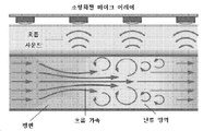
센서 어레이(100)는, 예를 들면, 협착 병변과 같은 혈관 시스템에서의 이상을 검출하기 위해 사용될 수 있다. 또한 도 4를 참조하면, 협착 병변은 협착 원위로 혈관 직경의 1 내지 3 배의 거리에서 난류 혈류를 야기할 수 있다. 난류 와류(turbulent vortex)는 협착도(DOS)에 관련되는 높은 피치(pitch)의 혈류 사운드를 생성할 수 있다. DOS는 혈관의 협착된 단면적 대 근위의 협착되지 않은 관강(lumen) 직경의 비율로서 정의될 수 있다. 몇몇 양태에 따르면, 협착은 DOS가 50%를 초과할 때 난류(turbulent flow)를 생성할 수 있다.The
본 명세서에서 개시되는 실시형태는 200 내지 1000㎐ 범위의 음향 주파수를 검출할 수 있는데, 이것은 청진기 다이어프램의 중립 대역폭(neutral bandwidth)을 초과할 수 있다. DOS는 다수의 기록 부위 또는 협착 위치에 대한 사전 지식을 사용한 근위 및 원위 기록의 비교에 의해 추정될 수 있다. 협착의 위치는 혈관 액세스를 따르는 복수의 부위에서의 기록 및 국소적 난류에 의해 야기되는 스펙트럼 변동의 영역의 검출을 통해 추정될 수 있다. 협착 위치가 검출되면, 스펙트럼 분석에 의해 DOS는 정량화될 수 있다.Embodiments disclosed herein may detect acoustic frequencies in the range of 200 to 1000 Hz, which may exceed the neutral bandwidth of the stethoscope diaphragm. DOS can be estimated by comparison of proximal and distal records using prior knowledge of multiple recording sites or stenosis locations. The location of the stenosis can be estimated through recording at multiple sites along the vascular access and detection of regions of spectral fluctuations caused by local turbulence. Once the location of the stenosis is detected, DOS can be quantified by spectral analysis.
환자의 혈관 액세스의 긴 길이, 구불구불하고, 가변적인 해부학적 구조에 기인하여, 정확한 PAG 기록을 위해 피부에 적합하기 위해서는 대규모의 유연한 마이크 어레이가 사용될 수 있다.Due to the long length, tortuous, and variable anatomy of the patient's vascular access, a large, flexible microphone array can be used to fit the skin for accurate PAG recording.
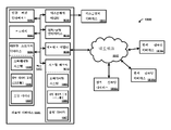
도 2 및 도 5 내지 도 7을 참조하면, 음향 센서 어레이(100)는, 음향 센서 어레이(100)로부터의 신호를, 디지털 신호 프로세싱을 수행하는 컴퓨팅 디바이스(1001)(도 35)로 제공할 수 있는 아날로그 프론트엔드(902) 및 데이터 컨버터(904)와 통신할 수 있다. 옵션 사항으로, 아날로그 프론트엔드(902)(예를 들면, 컨디셔닝 증폭기, 필터 등) 및 데이터 컨버터(904)는 제1 또는 제2 PCB(120 및 122) 중 하나 상에서 제공될 수 있다. 동일한 또는 별개의 컴퓨팅 디바이스(1001)는 데이터를 분석하기 위해 추가적인 데이터 프로세싱을 수행할 수 있다. 예를 들면, 컴퓨팅 디바이스(1001)는 음향 데이터로부터 피처를 추출할 수 있고, 센서 사이의 데이터를 비교할 수 있으며, 음향 데이터의 피처를 분류할 수 있다.2 and 5 to 7 , the
컴퓨팅 디바이스computing device
도 35는 센서 어레이(100)와의 사용을 위한 컴퓨팅 디바이스(1001)를 포함하는 시스템(1000)을 도시한다. 예시적인 양태에서, 컴퓨팅 디바이스(1001)는, 예를 들면, 퍼스널 컴퓨터, 컴퓨팅 스테이션(예를 들면, 워크스테이션), 랩탑 컴퓨터와 같은 휴대용 컴퓨터, 또는 서버일 수 있다.35 shows a
컴퓨팅 디바이스(1001)는 하나 이상의 프로세서(1003), 시스템 메모리(1012), 및 하나 이상의 프로세서(1003)를 포함하는 컴퓨팅 디바이스(1001)의 다양한 컴포넌트를 시스템 메모리(1012)에 커플링하는 버스(1013)를 포함할 수도 있다. 다수의 프로세서(1003)의 경우, 컴퓨팅 디바이스(1001)는 병렬 컴퓨팅을 활용할 수도 있다.Computing device 1001 includes one or
버스(1013)는, 다양한 버스 아키텍처 중 임의의 것을 사용하는 여러가지 가능한 타입의 버스 구조, 예컨대 메모리 버스, 메모리 컨트롤러, 주변장치 버스, 가속 그래픽 포트, 및 프로세서 또는 로컬 버스 중 하나 이상을 포함할 수도 있다.The bus 1013 may include several possible types of bus structures using any of a variety of bus architectures, such as one or more of a memory bus, a memory controller, a peripheral bus, an accelerated graphics port, and a processor or local bus. .
컴퓨팅 디바이스(1001)는 다양한 컴퓨터 판독 가능 매체(예를 들면, 비일시적) 상에서 동작할 수도 있고 그리고/또는 이들을 포함할 수도 있다. 컴퓨터 판독 가능 매체는 컴퓨팅 디바이스(1001)에 의해 액세스 가능한 임의의 이용 가능한 매체일 수도 있고, 비일시적, 휘발성 및/또는 불휘발성 매체, 착탈식 및 비착탈식 매체를 포함한다. 시스템 메모리(1012)는 랜덤 액세스 메모리(random access memory: RAM)와 같은 휘발성 메모리, 및/또는 판독 전용 메모리(read only memory: ROM)와 같은 불휘발성 메모리의 형태로 컴퓨터 판독 가능 매체를 갖는다. 시스템 메모리(1012)는 음향 데이터(1007)와 같은 데이터 및/또는 오퍼레이팅 시스템(1005) 및 하나 이상의 프로세서(1003)가 액세스 가능한 및/또는 그에 의해 동작되는 음향 데이터 분석 소프트웨어(1006)와 같은 프로그램 모듈을 저장할 수도 있다.The computing device 1001 may operate on and/or include various computer-readable media (eg, non-transitory). Computer-readable media may be any available media that can be accessed by computing device 1001 and includes non-transitory, volatile and/or non-volatile media, removable and non-removable media.
컴퓨팅 디바이스(1001)는 또한 다른 착탈식/비착탈식, 휘발성/불휘발성 컴퓨터 저장 매체를 포함할 수도 있다. 대용량 스토리지 디바이스(1004)는 컴퓨터 코드, 컴퓨터 판독 가능 명령어, 데이터 구조, 프로그램 모듈, 및 컴퓨팅 디바이스(1001)에 대한 다른 데이터의 불휘발성 저장을 제공할 수도 있다. 대용량 스토리지 디바이스(1004)는 하드 디스크, 착탈식 자기 디스크, 착탈식 광학 디스크, 자기 카세트 또는 다른 자기 스토리지 디바이스, 플래시 메모리 카드, CD-ROM, 디지털 다기능 디스크(digital versatile disk: DVD) 또는 다른 광학 스토리지, 랜덤 액세스 메모리(RAM), 판독 전용 메모리(ROM), 전기적으로 소거 가능한 프로그래머블 판독 전용 메모리(electrically erasable programmable read-only memory: EEPROM) 등일 수도 있다.The computing device 1001 may also include other removable/non-removable, volatile/nonvolatile computer storage media. Mass storage device 1004 may provide non-volatile storage of computer code, computer readable instructions, data structures, program modules, and other data for computing device 1001 . The mass storage device 1004 may include a hard disk, a removable magnetic disk, a removable optical disk, a magnetic cassette or other magnetic storage device, a flash memory card, a CD-ROM, a digital versatile disk (DVD) or other optical storage, random access memory (RAM), read-only memory (ROM), electrically erasable programmable read-only memory (EEPROM), or the like.
임의의 개수의 프로그램 모듈이 대용량 스토리지 디바이스(1004) 상에 저장될 수도 있다. 오퍼레이팅 시스템(1005) 및 음향 데이터 분석 소프트웨어(1006)는 대용량 스토리지 디바이스(1004) 상에 저장될 수도 있다. 오퍼레이팅 시스템(1005) 및 음향 데이터 분석 소프트웨어(1006) 중 하나 이상(또는 이들의 어떤 조합)은 프로그램 모듈 및 음향 데이터 분석 소프트웨어(1006)를 포함할 수도 있다. 음향 데이터(1007)는 또한 대용량 스토리지 디바이스(1004) 상에 저장될 수도 있다. 음향 데이터(1007)는 기술 분야에서 공지되어 있는 하나 이상의 데이터베이스 중 임의의 것에 저장될 수도 있다. 데이터베이스는 네트워크(1015) 내의 다수의 위치에 걸쳐 분산될 수 있거나 또는 중앙 집중화될 수도 있다.Any number of program modules may be stored on the mass storage device 1004 . The operating system 1005 and acoustic
유저는 입력 디바이스(도시되지 않음)를 통해 커맨드 및 정보를 컴퓨팅 디바이스(1001)에 입력할 수도 있다. 그러한 입력 디바이스는, 키보드, 포인팅 디바이스(예를 들면, 컴퓨터 마우스, 리모콘), 마이크, 조이스틱, 스캐너, 촉각 입력 디바이스 예컨대 장갑, 및 다른 신체 커버 용품, 모션 센서 등을 포함하지만, 그러나 이들로 제한되지는 않는다. 이들 및 다른 입력 디바이스는, 버스(1013)에 커플링되는 인간 머신 인터페이스(1002)를 통해 하나 이상의 프로세서(1003)에 연결될 수도 있지만, 그러나 병렬 포트, 게임 포트, IEEE 1394 포트(Firewire 포트로서 또한 공지되어 있음), 직렬 포트, 네트워크 어댑터(1008), 및/또는 범용 직렬 버스(universal serial bus: USB)와 같은 다른 인터페이스 및 버스 구조에 의해 연결될 수도 있다.A user may enter commands and information into the computing device 1001 via an input device (not shown). Such input devices include, but are not limited to, keyboards, pointing devices (eg, computer mice, remote controls), microphones, joysticks, scanners, tactile input devices such as gloves, and other body covering articles, motion sensors, and the like. does not These and other input devices may be coupled to one or
디스플레이 디바이스(1011)는 또한 디스플레이 어댑터(1009)와 같은 인터페이스를 통해 버스(1013)에 연결될 수도 있다. 컴퓨팅 디바이스(1001)는 하나보다 더 많은 디스플레이 어댑터(1009)를 가질 수도 있고 컴퓨팅 디바이스(1001)는 하나보다 더 많은 디스플레이 디바이스(1011)를 가질 수도 있다는 것이 고려된다. 디스플레이 디바이스(1011)는 모니터, LCD(Liquid Crystal Display), 발광 다이오드(light emitting diode: LED) 디스플레이, 텔레비전, 스마트 렌즈, 스마트 글래스, 및/또는 프로젝터일 수도 있다. 디스플레이 디바이스(1011)에 추가하여, 다른 출력 주변장치 디바이스는 입력/출력 인터페이스(1010)를 통해 컴퓨팅 디바이스(1001)에 연결될 수도 있는 스피커(도시되지 않음) 및 프린터(도시되지 않음)와 같은 컴포넌트를 포함할 수도 있다. 방법의 임의의 단계 및/또는 결과는 출력 디바이스에 임의의 형태로 출력될 수도 있다(또는 출력되게 될 수도 있다). 그러한 출력은, 텍스트, 그래픽, 애니메이션, 오디오, 촉각, 및 등등을 포함하는, 그러나 이들로 제한되지는 않는 임의의 형태의 시각적 표현일 수도 있다. 디스플레이(1011) 및 컴퓨팅 디바이스(1001)는 하나의 디바이스의 일부일 수도 있거나, 또는 별개의 디바이스일 수도 있다.
컴퓨팅 디바이스(1001)는 하나 이상의 원격 컴퓨팅 디바이스(1014a,b,c)에 대한 논리적 연결을 사용하여 네트워크화된 환경에서 동작할 수도 있다. 원격 컴퓨팅 디바이스(1014a,b,c)는 퍼스널 컴퓨터, 컴퓨팅 스테이션(예를 들면, 워크스테이션), 휴대용 컴퓨터(예를 들면, 랩탑, 이동 전화, 태블릿 디바이스), 스마트 디바이스(예를 들면, 스마트폰, 스마트 워치, 활동 추적기, 스마트 의류, 스마트 액세서리), 보안 및/또는 모니터링 디바이스, 서버, 라우터, 네트워크 컴퓨터, 피어 디바이스, 에지 디바이스 또는 다른 공통 네트워크 노드, 및 등등일 수도 있다. 컴퓨팅 디바이스(1001)와 원격 컴퓨팅 디바이스(1014a,b,c) 사이의 논리적 연결은 근거리 통신망(local area network: LAN) 및/또는 일반적인 광역 통신망(wide area network: WAN)과 같은 네트워크(1015)를 통해 이루어질 수도 있다. 그러한 네트워크 연결은 네트워크 어댑터(1008)를 통할 수도 있다. 네트워크 어댑터(1008)는 유선 및 무선 환경 둘 모두에서 구현될 수도 있다. 그러한 네트워킹 환경은 일반적이고 주거지, 사무실, 전사적 컴퓨터 네트워크, 인트라넷, 및 인터넷에서는 평범하다.The computing device 1001 may operate in a networked environment using logical connections to one or more
오퍼레이팅 시스템(1005)과 같은 애플리케이션 프로그램 및 다른 실행 가능한 프로그램 컴포넌트는 본 명세서에서 별개의 블록으로서 도시되지만, 그러한 프로그램 및 컴포넌트는 컴퓨팅 디바이스(1001)의 상이한 스토리지 컴포넌트에서 다양한 시간에 존재할 수도 있고, 컴퓨팅 디바이스(1001)의 하나 이상의 프로세서(1003)에 의해 실행된다는 것이 인식된다. 음향 데이터 분석 소프트웨어(1006)의 구현은 어떤 형태의 컴퓨터 판독 가능 매체 상에 저장될 수도 있거나 또는 그들을 통해 전송될 수도 있다. 개시된 방법 중 임의의 것은 컴퓨터 판독 가능 매체 상에서 구체화되는 프로세서 실행 가능 명령어에 의해 수행될 수도 있다.Although application programs and other executable program components, such as operating system 1005 , are shown herein as separate blocks, such programs and components may reside at various times in different storage components of computing device 1001 , and the computing device It is recognized that execution by one or
머신 러닝machine learning
컴퓨팅 디바이스(1001)는 메모리 모듈과 통신하는 머신 러닝 모듈을 포함할 수 있다.The computing device 1001 may include a machine learning module in communication with a memory module.
이제 도 55를 참조하면, 시스템(800)이 도시되어 있다. 시스템(800)은, 트레이닝 모듈(820)에 의한 하나 이상의 트레이닝 데이터 세트(810A 내지 810B)의 분석에 기초하여, 협착도 범위(예를 들면, 경증, 중등증 또는 중증)를 나타내는 것으로서 음향 신호를 분류하도록 구성되는 적어도 하나의 머신 러닝 기반의 분류기(830)를 트레이닝시키기 위해 머신 러닝 기술을 사용하도록 구성될 수도 있다. 트레이닝 데이터 세트(810A)(예를 들면, 하나 이상의 센서로부터의 음향 데이터의 제1 부분)는 음향 피처 및 음향 피처가 나타내는 관련된 협착도를 포함할 수 있다. 트레이닝 데이터 세트(810B)(예를 들면, 하나 이상의 센서로부터의 음향 데이터의 제2 부분)는 음향 피처 및 음향 피처가 나타내는 관련된 협착도를 포함할 수 있다. 라벨은 "경증 협착", "중등증 협착" 및 "중증 협착"을 포함할 수도 있다.Referring now to FIG. 55 , a
하나 이상의 센서로부터의 음향 데이터의 제2 부분은 트레이닝 데이터 세트(810B)에 또는 테스팅 데이터 세트에 랜덤하게 할당될 수 있다. 몇몇 구현예에서, 트레이닝 데이터 세트 또는 테스팅 데이터 세트에 대한 데이터의 할당은 완전히 랜덤하지는 않을 수도 있다. 이 경우, 할당 동안 하나 이상의 기준, 예컨대 트레이닝 및 테스팅 데이터 세트 각각에서 상이한 관련된 협착도를 갖는 유사한 개수의 음향 데이터 피처가 있는 것을 보장하는 것이 사용될 수도 있다. 일반적으로, 트레이닝 데이터 세트 및 테스팅 데이터 세트에서 충분한 품질과 불충분한 품질 라벨의 분포가 어느 정도 유사한 것을 보장하면서, 데이터를 트레이닝 또는 테스팅 데이터 세트에 할당하기 위해 임의의 적절한 방법이 사용될 수도 있다.The second portion of acoustic data from the one or more sensors may be randomly assigned to the training data set 810B or to the testing data set. In some implementations, the allocation of data to a training data set or a testing data set may not be completely random. In this case, one or more criteria during assignment may be used, such as ensuring that there is a similar number of acoustic data features with different associated stenosis in each of the training and testing data sets. In general, any suitable method may be used to assign data to a training or testing data set, while ensuring that the distribution of sufficient quality and insufficient quality labels in the training data set and the testing data set is somewhat similar.
트레이닝 모듈(820)은, 하나 이상의 피처 선택 기술에 따라 트레이닝 데이터 세트(810A) 내의 하나 이상의 센서로부터의 음향 데이터의 제1 부분으로부터 피처 세트를 추출하는 것에 의해 머신 러닝 기반의 분류기(830)를 트레이닝시킬 수도 있다. 트레이닝 모듈(820)은 또한, 포지티브 예(positive example)의 통계적으로 유의미한 피처(예를 들면, 주어진 DOS의 특정한 속성(들)을 묘사하는 피처) 및 네거티브 예(negative example)의 통계적으로 유의미한 피처(예를 들면, 주어진 DOS 외부의 특정한 속성(들)을 묘사하는 피처)를 포함하는 트레이닝 데이터 세트(810B) 내의 하나 이상의 센서로부터의 음향 데이터의 제2 부분에 하나 이상의 피처 선택 기술을 적용하는 것에 의해 트레이닝 데이터 세트(810A)로부터 획득되는 피처 세트를 추가로 정의할 수도 있다.The
트레이닝 모듈(820)은 트레이닝 데이터 세트(810A) 및/또는 트레이닝 데이터 세트(810B)로부터 다양한 방식으로 피처 세트를 추출할 수도 있다. 트레이닝 모듈(820)은, 매번 상이한 피처 추출 기술을 사용하여 피처 추출을 다수 회 수행할 수도 있다. 한 실시형태에서, 상이한 기술을 사용하여 생성되는 피처 세트는 상이한 머신 러닝 기반의 분류 모델(840)을 생성하기 위해 각각 사용될 수도 있다. 예를 들면, 최고 품질 메트릭을 갖는 피처 세트가 트레이닝에서의 사용을 위해 선택될 수도 있다. 트레이닝 모듈(820)은, 새로운 음향 데이터 피처가 대응하는 DOS의 특정한 속성(들)을 묘사하는 피처를 포함하는지 또는 포함하지 않는지의 여부를 나타내도록 구성되는 하나 이상의 머신 러닝 기반의 분류 모델(840A 내지 840N)을 구축하기 위해 피처 세트(들)를 사용할 수도 있다.The
트레이닝 데이터 세트(810A) 및/또는 트레이닝 데이터 세트(810B)는, 트레이닝 데이터 세트(810A) 및/또는 트레이닝 데이터 세트(810B)에서 충분한 품질/불충분한 품질 라벨과 추출된 피처 사이의 임의의 종속성, 관련성 및/또는 상관 관계를 결정하기 위해 분석될 수도 있다. 식별된 상관 관계는, 대응하는 음향 데이터 세트의 특정한 속성(들)을 묘사하는 음향 피처에 대한 라벨 및 대응하는 DOS의 특정한 속성(들)을 묘사하지 않는 음향 피처에 대한 라벨과 관련되는 피처의 목록의 형태를 가질 수도 있다. 피처는 머신 러닝 컨텍스트에서 변수로서 간주될 수도 있다. 용어 "피처"는, 본 명세서에서 사용되는 바와 같이, 데이터의 아이템이 하나 이상의 특정한 카테고리에 속하는지의 여부를 결정하기 위해 사용될 수도 있는 데이터의 아이템의 임의의 특성을 지칭할 수도 있다. 예로서, 본 명세서에서 설명되는 피처는 하나 이상의 음향 피처 속성을 포함할 수도 있다. 하나 이상의 음향 피처 속성은, 예를 들면, 청각 스펙트럼 중심(ASC, 본 명세서에서 추가로 설명됨)의 수축기 세그먼트의 적어도 일부에 관련되는 값(예를 들면, 그 일부의 평균) 및 청각 스펙트럼 플럭스(ASF, 본 명세서에서 추가로 설명됨)의 수축기 세그먼트의 적어도 일부의 값(예를 들면, 그 일부의 RSM)을 포함할 수도 있다.Training data set 810A and/or training data set 810B may contain any dependencies between sufficient quality/poor quality labels and extracted features in training data set 810A and/or training data set 810B; It may be analyzed to determine relevance and/or correlation. The identified correlation is a list of features associated with a label for an acoustic feature that depicts specific attribute(s) of the corresponding acoustic data set and a label for an acoustic feature that does not depict the specific attribute(s) of the corresponding DOS. may have the form of A feature may be considered as a variable in a machine learning context. The term “feature,” as used herein, may refer to any characteristic of an item of data that may be used to determine whether the item of data belongs to one or more particular categories. By way of example, a feature described herein may include one or more acoustic feature attributes. The one or more acoustic feature attributes may include, for example, a value (e.g., an average of a portion) and an auditory spectral flux ( values of at least a portion of the systolic segment of the ASF (described further herein) (eg, the RSM of that portion).
피처 선택 기술은 하나 이상의 피처 선택 규칙을 포함할 수도 있다. 하나 이상의 피처 선택 규칙은 음향 피처 속성 및 음향 피처 속성 발생 규칙을 포함할 수도 있다. 음향 피처 속성 발생 규칙은, 트레이닝 데이터 세트(810A)에서 어떤 음향 피처 속성이 임계 횟수를 넘어 발생하는지를 결정하는 것 및 임계치를 충족하는 그들 음향 피처 속성을 후보 피처로서 식별하는 것을 포함할 수도 있다. 예를 들면, 트레이닝 데이터 세트(810A)에서 8회보다 더 많이 또는 동등하게 나타나는 임의의 음향 피처 속성이 후보 피처로서 고려될 수도 있다. 8회 미만으로 나타나는 임의의 음향 피처 속성은 피처로서의 고려로부터 배제될 수도 있다. 필요에 따라 임의의 임계량이 사용될 수도 있다.A feature selection technique may include one or more feature selection rules. The one or more feature selection rules may include acoustic feature attributes and acoustic feature attribute generation rules. The acoustic feature attribute generation rules may include determining which acoustic feature attributes occur beyond a threshold number of times in the training data set 810A and identifying those acoustic feature attributes that meet the threshold as candidate features. For example, any acoustic feature attribute that appears more than or equal to eight times in the training data set 810A may be considered a candidate feature. Any acoustic feature attribute that appears less than 8 times may be excluded from consideration as a feature. Any threshold amount may be used as needed.
피처를 선택하기 위해 단일의 피처 선택 규칙이 적용될 수도 있거나 또는 피처를 선택하기 위해 다수의 피처 선택 규칙이 적용될 수도 있다. 피처 선택 규칙은, 피처 선택 규칙이 특정한 순서로 적용되고 이전 규칙의 결과에 적용되는 종속 접속 양식(cascading fashion)으로 적용될 수도 있다. 예를 들면, 음향 피처 속성 발생 규칙은 음향 피처 속성의 제1 목록을 생성하기 위해 트레이닝 데이터 세트(810A)에 적용될 수도 있다. 후보 피처의 최종 목록은 하나 이상의 후보 그룹(예를 들면, 음향 피처 속성의 그룹)을 결정하기 위해 추가적인 피처 선택 기술에 따라 분석될 수도 있다. 필터, 래퍼(wrapper), 및/또는 임베딩된 방법과 같은 임의의 피처 선택 기술을 사용하여 후보 피처 그룹을 식별하기 위해 임의의 적절한 계산 기술이 사용될 수도 있다. 필터 방법에 따라 하나 이상의 후보 피처 그룹이 선택될 수도 있다. 필터 방법은, 예를 들면, 피어슨(Pearson) 상관, 선형 판별 분석, 분산의 분석(analysis of variance: ANOVA), 카이 제곱(chi-square), 이들의 조합, 및 등등을 포함한다. 필터 방법에 따른 피처의 선택은 임의의 머신 러닝 알고리즘과는 독립적이다. 대신, 피처는 결과 변수(예를 들면, 대응하는 음향 데이터 샘플의 특정한 속성(들)을 묘사하는 또는 묘사하지 않는 음향 피처)와의 그들의 상관 관계에 대한 다양한 통계적 테스트에서의 점수에 기초하여 선택될 수도 있다.A single feature selection rule may be applied to select a feature, or multiple feature selection rules may be applied to select a feature. Feature selection rules may be applied in a cascading fashion where feature selection rules are applied in a particular order and applied to the results of previous rules. For example, acoustic feature attribute generation rules may be applied to training data set 810A to generate a first list of acoustic feature attributes. The final list of candidate features may be analyzed according to additional feature selection techniques to determine one or more candidate groups (eg, groups of acoustic feature attributes). Any suitable computational technique may be used to identify a group of candidate features using any feature selection technique, such as filters, wrappers, and/or embedded methods. One or more candidate feature groups may be selected according to the filter method. Filter methods include, for example, Pearson correlation, linear discriminant analysis, analysis of variance (ANOVA), chi-square, combinations thereof, and the like. The selection of features according to the filter method is independent of any machine learning algorithm. Instead, features may be selected based on scores in various statistical tests for their correlation with outcome variables (eg, acoustic features that depict or do not depict particular attribute(s) of the corresponding acoustic data sample). have.
다른 예로서, 래퍼 방법에 따라 하나 이상의 후보 피처 그룹이 선택될 수도 있다. 래퍼 방법은 피처의 서브세트를 사용하도록 그리고 피처의 서브세트를 사용하여 머신 러닝 모델을 트레이닝시키도록 구성될 수도 있다. 이전 모델로부터 인출된 추론에 기초하여, 피처가 서브세트에 추가될 수도 있고 그리고/또는 그로부터 삭제될 수도 있다. 래퍼 방법은, 예를 들면, 순방향 피처 선택, 역방향 피처 제거, 재귀적 피처 제거, 이들의 조합, 및 등등을 포함한다. 한 실시형태에서, 순방향 피처 선택은 하나 이상의 후보 피처 그룹을 식별하기 위해 사용될 수도 있다. 순방향 피처 선택은 머신 러닝 모델의 피처 없이 시작하는 반복적인 방법이다. 각각의 반복에서, 새로운 피처의 추가가 머신 러닝 모델의 성능이 향상시키지 않을 때까지, 모델을 최상으로 향상시키는 피처가 추가된다. 한 실시형태에서, 하나 이상의 후보 피처 그룹을 식별하기 위해 역방향 제거가 사용될 수도 있다. 역방향 제거는 머신 러닝 모델의 모든 피처를 가지고 시작하는 반복적인 방법이다. 각각의 반복에서, 피처의 제거시 어떠한 개선도 관찰되지 않을 때까지, 가장 덜 중요한 피처가 제거된다. 재귀적 피처 제거는 하나 이상의 후보 피처 그룹을 식별하기 위해 사용될 수도 있다. 재귀적 피처 제거는 최상의 성능의 피처 서브세트를 찾는 것을 목표로 하는 탐욕적인 최적화 알고리즘(greedy optimization algorithm)이다. 재귀적 피처 제거는 모델을 반복적으로 생성하고 각각의 반복에서의 최상의 또는 최악의 성능의 피처를 따로 보관한다. 재귀적 피처 제거는 모든 피처가 소진될 때까지 남아 있는 피처를 갖는 다음 번 모델을 구성한다. 그 다음, 재귀적 피처 제거는 그들의 제거의 순서에 기초하여 피처를 평가한다(rank).As another example, one or more groups of candidate features may be selected according to the wrapper method. The wrapper method may be configured to use a subset of features and to train a machine learning model using the subset of features. Based on inferences drawn from previous models, features may be added to and/or deleted from the subset. Wrapper methods include, for example, forward feature selection, backward feature removal, recursive feature removal, combinations thereof, and the like. In one embodiment, forward feature selection may be used to identify one or more groups of candidate features. Forward feature selection is an iterative method that starts without features in a machine learning model. At each iteration, the features that best improve the model are added, until adding new features does not improve the performance of the machine learning model. In an embodiment, reverse removal may be used to identify one or more groups of candidate features. Reverse elimination is an iterative method that starts with all the features of a machine learning model. At each iteration, the least important features are removed until no improvement is observed upon removal of the features. Recursive feature removal may be used to identify one or more groups of candidate features. Recursive feature removal is a greedy optimization algorithm that aims to find the best performing subset of features. Recursive feature removal iteratively builds the model and sets aside the best or worst performing features at each iteration. Recursive feature removal constructs the next model with the remaining features until all features are exhausted. Recursive feature removal then ranks features based on the order of their removal.
추가적인 예로서, 하나 이상의 후보 피처 그룹이 임베딩된 방법에 따라 선택될 수도 있다. 임베딩된 방법은 필터 및 래퍼 방법의 품질을 결합한다. 임베딩된 방법은, 예를 들면, 과적합을 감소시키기 위해 벌점 기능(penalization function)을 구현하는 최소 절대 수축 및 선택 연산자(Least Absolute Shrinkage and Selection Operator: LASSO) 및 리지 회귀(ridge regression)를 포함한다. 예를 들면, LASSO 회귀는, 계수의 크기의 절대 값과 등가인 페널티를 추가하는 L1 정규화(regularization)를 수행하고, 리지 회귀는 계수의 크기의 제곱과 등가인 페널티를 추가하는 L2 정규화를 수행한다.As a further example, one or more groups of candidate features may be selected according to how they are embedded. The embedded method combines the qualities of a filter and wrapper method. Embedded methods include, for example, Least Absolute Shrinkage and Selection Operator (LASSO) and ridge regression that implement a penalty function to reduce overfitting. . For example, LASSO regression performs L1 regularization that adds a penalty equal to the absolute value of the magnitude of the coefficient, and ridge regression performs L2 regularization that adds a penalty equal to the square of the magnitude of the coefficient .
트레이닝 모듈(820)이 피처 세트(들)를 생성한 이후, 트레이닝 모듈(820)은 피처 세트(들)에 기초하여 머신 러닝 기반의 분류 모델(840)을 생성할 수도 있다. 머신 러닝 기반의 분류 모델은 머신 러닝 기술을 사용하여 생성되는 데이터 분류를 위한 복잡한 수학적 모델을 지칭할 수도 있다. 일례에서, 이 머신 러닝 기반의 분류기는 경계 피처를 나타내는 서포트 벡터의 맵을 포함할 수도 있다. 예로서, 경계 피처는 피처 세트로부터 선택될 수도 있고, 그리고/또는 피처 세트에서 가장 높게 평가된 피처를 나타낼 수도 있다.After the
트레이닝 모듈(820)은, 각각의 분류 카테고리(예를 들면, 대응하는 음향 데이터 세트의 각각의 속성)에 대한 머신 러닝 기반의 분류 모델(840A-840N)을 구축하기 위해, 트레이닝 데이터 세트(810A) 및/또는 트레이닝 데이터 세트(810B)로부터 추출되는 피처 세트를 사용할 수도 있다. 몇몇 예에서, 머신 러닝 기반의 분류 모델(840A-840N)은 단일의 머신 러닝 기반의 분류 모델(840)로 결합될 수도 있다. 유사하게, 머신 러닝 기반의 분류기(830)는 단일의 또는 복수의 머신 러닝 기반의 분류 모델(840)을 포함하는 단일의 분류기 및/또는 단일의 또는 복수의 머신 러닝 기반의 분류 모델(840)을 포함하는 다수의 분류기를 나타낼 수도 있다.The
추출된 피처(예를 들면, 하나 이상의 음향 피처 속성)는, 판별 분석; 결정 트리; 최근접 이웃(nearest neighbor: NN) 알고리즘(예를 들면, k-NN 모델, 리플리케이터 NN 모델 등); 통계적 알고리즘(예를 들면, Bayesian(베이지안) 네트워크 등); 클러스터링 알고리즘(예를 들면, k-평균(k-means), 평균 시프트 등); 신경망(예를 들면, 저장소 네트워크(reservoir network), 인공 신경망 등); 서포트 벡터 머신(support vector machine: SVM); 로지스틱 회귀 알고리즘(logistic regression algorithm); 선형 회귀 알고리즘; 마르코프(Markov) 모델 또는 체인; 주 성분 분석(principal component analysis: PCA)(예를 들면, 선형 모델용); 다중 층 퍼셉트론(multi-layer perceptron: MLP) ANN(예를 들면, 비선형 모델용); 복제 저장소 네트워크(replicating reservoir network)(예를 들면, 비선형 모델용, 통상적으로 시계열의 경우); 랜덤 포레스트 분류(random forest classification); 이들의 조합 및/또는 등등과 같은 머신 러닝 접근법을 사용하여 트레이닝되는 분류 모델에서 결합될 수도 있다. 결과적으로 나타나는 머신 러닝 기반의 분류기(830)는 음향 피처(들)를 (예를 들면, 대응하는 음향 데이터 세트의 특정한 속성(들)을 묘사하는 또는 묘사하지 않는) 클래스에 할당하기 위해 각각의 후보 음향 피처 속성에 대한 결정 규칙 또는 매핑을 포함할 수도 있다.The extracted features (eg, one or more acoustic feature attributes) may be subjected to discriminant analysis; decision tree; nearest neighbor (NN) algorithms (eg, k-NN model, replicator NN model, etc.); statistical algorithms (eg, Bayesian networks, etc.); clustering algorithms (eg, k-means, mean shift, etc.); neural networks (eg, reservoir networks, artificial neural networks, etc.); support vector machine (SVM); logistic regression algorithm; linear regression algorithm; Markov model or chain; principal component analysis (PCA) (eg, for linear models); multi-layer perceptron (MLP) ANNs (eg, for non-linear models); replicating reservoir networks (eg for non-linear models, typically for time series); random forest classification; combinations thereof and/or may be combined in a classification model that is trained using machine learning approaches, such as and/or the like. The resulting machine learning-based
후보 음향 피처 속성 및 머신 러닝 기반의 분류기(830)는 (예를 들면, 제2 음향 데이터 세트의 제2 부분에서) 테스팅 데이터 세트에 대한 (예를 들면, 특정한 DOS에 대응하는) 라벨을 예측하기 위해 사용될 수도 있다. 일례에서, 각각의 테스팅 데이터 세트에 대한 예측은, 대응하는 음향 피처가 특정한 DOS를 묘사할 또는 묘사하지 않을 가능성 또는 확률에 대응하는 신뢰도 레벨을 포함한다. 신뢰도 레벨은 0과 1 사이의 값일 수도 있고, 이것은 대응하는 음향 피처(들)가 특정한 클래스에 속할 가능성을 나타낼 수도 있다. 일례에서, 두 가지 상태(예를 들면, 대응하는 음향 데이터 세트의 특정한 속성(들)을 묘사함 또는 묘사하지 않음)가 있을 때, 신뢰도 레벨은, 특정한 음향 피처가 제1 상태(예를 들면, 특정한 속성(들)을 묘사함)에 속할 가능성을 가리키는 값 p에 대응할 수도 있다. 이 경우, 값 1 - p는 특정한 음향 피처가 제2 상태(예를 들면, 특정한 속성(들)을 묘사하지 않음)에 속할 가능성을 가리킬 수도 있다. 일반적으로, 두 개보다 더 많은 상태가 있을 때 각각의 음향 피처에 대해 그리고 각각의 후보 음향 피처 속성에 대해 다수의 신뢰도 레벨이 제공될 수도 있다. 최고 성능의 후보 음향 피처 속성은 각각의 음향 피처에 대해 획득되는 결과를, 테스팅 데이터 세트의 각각의 대응하는 음향 데이터 세트에 대한 공지된 충분한 품질/불충분한 품질 상태와 비교하는 것에 의해(예를 들면, 각각의 음향 피처에 대해 획득되는 결과를, 하나 이상의 센서로부터의 음향 데이터의 제2 부분의 라벨링된 음향 데이터와 비교하는 것에 의해) 결정될 수도 있다. 일반적으로, 대응하는 음향 데이터의 특정한 속성(들)에 대한 최고 성능의 후보 음향 피처 속성은 공지된 묘사 상태 또는 비묘사 상태와 밀접하게 매치하는 결과를 가질 것이다.The candidate acoustic feature attribute and machine learning-based
최고 성능의 음향 피처 속성은 새로운 음향 데이터 세트의 음향 피처에 기초하여 DOS를 예측하기 위해 사용될 수도 있다. 예를 들면, 새로운 음향 데이터 세트가 결정/수신될 수도 있다. 새로운 음향 데이터 세트는, 대응하는 음향 데이터의 특정한 속성(들)에 대한 최고 성능의 음향 피처 속성에 기초하여, 새로운 음향 데이터 세트의 음향 피처를, 특정한 속성(들)을 포함하는 것으로 또는 포함하지 않는 것으로 분류할 수도 있는 머신 러닝 기반의 분류기(830)에 제공될 수도 있다.The best performing acoustic feature properties may be used to predict DOS based on acoustic features in a new acoustic data set. For example, a new set of acoustic data may be determined/received. The new acoustic data set contains the acoustic features of the new acoustic data set with or without the specific attribute(s), based on the best performing acoustic feature attribute for the specific attribute(s) of the corresponding acoustic data. It may also be provided to a machine learning-based
애플리케이션은, 분할 마스크(또는 임의의 생성된 또는 삭제된 속성)에 의해 나타내어지는 속성 중 임의의 것에 대해 이루어지는 하나 이상의 유저 편집의 지시(indication)를 컴퓨팅 디바이스(1001)에 제공할 수도 있다. 예를 들면, 유저는, 속성(들)의 경계의 묘사를 최적으로 묘사하기 위해, 분할 마스크에 의해 나타내어지는 속성 중 임의의 것을, 마우스 움직임을 통해 그의 포인트 중 일부를 소망되는 포지션으로 드래그하는 것에 의해, 편집할 수도 있다. 다른 예로서, 유저는 마우스를 통해 분할 마스크의 일부를 묘화하거나 또는 다시 묘화할 수도 있다. 유저 커맨드를 획득하는 다른 입력 디바이스 또는 방법이 또한 사용될 수도 있다. 하나 이상의 유저 편집은 의미론적 분할 모델을 최적화하기 위해 머신 러닝 모듈에 의해 사용될 수도 있다. 예를 들면, 트레이닝 모듈(820)은 하나 이상의 유저 편집을 포함하는 출력 데이터 세트로부터 하나 이상의 피처를 추출할 수도 있다. 트레이닝 모듈(820)은, 머신 러닝 기반의 분류기(830)를 재트레이닝시키기 위해 그리고 그에 의해 머신 러닝 기반의 분류기(830)에 의해 제공되는 결과를 지속적으로 개선하기 위해, 하나 이상의 피처를 사용할 수도 있다.The application may provide the computing device 1001 with an indication of one or more user edits made to any of the attributes indicated by the segmentation mask (or any created or deleted attributes). For example, the user may drag any of the attributes represented by the segmentation mask to the desired position via mouse movement to optimally depict the depiction of the boundary of the attribute(s). It can also be edited by As another example, the user may draw or redraw a portion of the segmentation mask via the mouse. Other input devices or methods of obtaining user commands may also be used. One or more user edits may be used by the machine learning module to optimize the semantic segmentation model. For example, the
이제 도 9로 돌아가면, 예시적인 트레이닝 방법(900)을 예시하는 플로우차트가 도시되어 있다. 방법(900)은 트레이닝 모듈(820)을 사용하여 머신 러닝 기반의 분류기(830)를 생성하기 위해 사용될 수도 있다. 트레이닝 모듈(820)은 감독(supervised), 자율(unsupervised), 및/또는 반감독(semi-supervised)(예를 들면, 보강 기반) 머신 러닝 기반의 분류 모델(840)을 구현할 수 있다. 도 9에서 예시되는 방법(900)은, 감독 학습 방법의 한 예이다; 트레이닝 방법의 이 예의 변형예가 하기에서 논의되지만, 그러나, 다른 트레이닝 방법은 자율 및/또는 반감독 머신 러닝 모델을 트레이닝시키기 위해 유사하게 구현될 수 있다.Turning now to FIG. 9 , a flowchart illustrating an
트레이닝 방법(900)은, 단계(910)에서, 복수의 음향 피처와 관련되는 제1 음향 데이터 세트(예를 들면, 제1 음향 데이터 샘플) 및 복수의 음향 피처와 관련되는 제2 음향 데이터 세트(예를 들면, 제2 음향 데이터 샘플)를 결정(예를 들면, 액세스, 수신, 검색 등)할 수도 있다. 제1 음향 데이터 세트 및 제2 음향 데이터 세트 각각은, 음향 피처와 관련되는 하나 이상의 음향 결과 데이터세트를 포함할 수도 있고, 각각의 음향 결과 데이터세트는 특정한 속성과 관련될 수도 있다. 각각의 음향 결과 데이터 세트는 음향 결과의 라벨링된 목록을 포함할 수도 있다. 라벨은 "경증 협착", "중등증 협착 및 중증 협착"을 포함할 수도 있다.The
트레이닝 방법(900)은, 단계(920)에서, 트레이닝 데이터 세트 및 테스팅 데이터 세트를 생성할 수도 있다. 트레이닝 데이터 세트 및 테스팅 데이터 세트는, 제2 음향 데이터 세트로부터의 라벨링된 이미징 결과를, 트레이닝 데이터 세트 또는 테스팅 데이터 세트 중 어느 하나에 랜덤하게 할당하는 것에 의해 생성될 수도 있다. 몇몇 구현예에서, 트레이닝 또는 테스트 샘플로서의 라벨링된 이미징 결과의 할당은 완전히 랜덤은 아닐 수도 있다. 한 실시형태에서, 특정한 DOS 타입 및/또는 클래스에 대한 라벨링된 음향 결과만이 트레이닝 데이터 세트 및 테스팅 데이터 세트를 생성하기 위해 사용될 수도 있다. 한 실시형태에서, 특정한 DOS 타입 및/또는 클래스에 대한 라벨링된 음향 결과의 대부분은 트레이닝 데이터 세트를 생성하기 위해 사용될 수도 있다. 예를 들면, 특정한 DOS 타입 및/또는 클래스에 대한 라벨링된 음향 결과의 75%는 트레이닝 데이터 세트를 생성하기 위해 사용될 수도 있고 25%는 테스팅 데이터 세트를 생성하기 위해 사용될 수도 있다.The
트레이닝 방법(900)은, 단계(930)에서, 예를 들면, 상이한 분류(예를 들면, "경증 협착", "중등증 협착", 또는 "중증 협착") 사이를 구별하기 위해 분류기에 의해 사용될 수 있는 하나 이상의 피처를 결정(예를 들면, 추출, 선택 등)할 수도 있다. 하나 이상의 피처는 음향 데이터 결과 속성의 세트를 포함할 수도 있다. 한 실시형태에서, 트레이닝 방법(900)은 제1 음향 데이터 세트로부터 세트 피처를 결정할 수도 있다. 다른 실시형태에서, 트레이닝 방법(900)은 제2 음향 데이터 세트로부터 피처의 세트를 결정할 수도 있다. 또 다른 실시형태에서, 피처의 세트는, 트레이닝 데이터 세트 및 테스팅 데이터 세트의 라벨링된 이미징 결과와 관련되는 DOS 타입 및/또는 클래스와는 상이한 DOS 타입 및/또는 클래스로부터의 라벨링된 이미징 결과로부터 결정될 수도 있다. 다시 말하면, 상이한 DOS 타입 및/또는 클래스로부터의 라벨링된 이미징 결과는, 머신 러닝 모델을 트레이닝시키기 보다는, 피처 결정을 위해 사용될 수도 있다. 트레이닝 데이터 세트는, 하나 이상의 피처를 결정하기 위해, 상이한 DOS 타입 및/또는 클래스로부터의 라벨링된 이미징 결과와 연계하여 사용될 수도 있다. 상이한 DOS 타입 및/또는 클래스로부터의 라벨링된 이미징 결과는, 트레이닝 데이터 세트를 사용하여 추가로 감소될 수도 있는 피처의 초기 세트를 결정하기 위해 사용될 수도 있다.The
트레이닝 방법(900)은, 단계(940)에서, 하나 이상의 피처를 사용하여 하나 이상의 머신 러닝 모델을 트레이닝시킬 수도 있다. 하나의 실시형태에서, 머신 러닝 모델은 감독 학습을 사용하여 트레이닝될 수도 있다. 다른 실시형태에서, 자율 학습 및 반감독 학습을 비롯한, 다른 머신 러닝 기술이 활용될 수도 있다. (940)에서 트레이닝되는 머신 러닝 모델은, 해결될 문제 및/또는 트레이닝 데이터 세트에서 이용 가능한 데이터에 따라 상이한 기준에 기초하여 선택될 수도 있다. 예를 들면, 머신 러닝 분류기는 상이한 정도의 편향을 겪을 수 있다. 따라서, 하나보다 더 많은 머신 러닝 모델이, (940)에서, 트레이닝될 수 있고, 그 다음, 단계(950)에서, 최적화, 개선 및 교차 유효성 확인될 수 있다.The
트레이닝 방법(900)은, (960)에서, 예측 모델(예를 들면, 머신 러닝 분류기)을 구축하기 위해 하나 이상의 머신 러닝 모델을 선택할 수도 있다. 예측 모델은 테스팅 데이터 세트를 사용하여 평가될 수도 있다. 예측 모델은, 단계(970)에서, 테스팅 데이터 세트를 분석할 수도 있고 분류 값 및/또는 예측된 값을 생성할 수도 있다. 분류 및/또는 예측 값은, 그러한 값이 소망되는 정확도 레벨을 달성하였는지의 여부를 결정하기 위해, 단계(980)에서, 평가될 수도 있다.The
본 명세서에서 설명되는 예측 모델의 성능은, 음향 데이터 세트의 음향 피처의 다수의 진양성(true positive), 위양성(false positive), 진음성(true negative), 및/또는 위음성(false negative) 분류에 기초하여 다수의 방식으로 평가될 수도 있다. 예를 들면, 예측 모델의 위양성은, 실제로 특정한 속성을 묘사하지 않았던 특정한 속성을 묘사하는 것으로 예측 모델이 음향 피처(들)를 잘못 분류한 횟수를 가리킬 수도 있다. 반대로, 머신 러닝 모델(들)의 위음성은, 실제로, 하나 이상의 음향 피처가 특정한 속성을 묘사할 때, 예측 모델이 음향 데이터 세트의 하나 이상의 음향 피처를, 특정한 속성을 묘사하지 않는 것으로 분류한 횟수를 가리킬 수도 있다. 진음성 및 진양성은, 예측 모델이 음향 데이터 세트의 하나 이상의 음향 피처를, 특정한 속성을 충분히 묘사하는 것으로 또는 특정한 속성을 묘사하지 않는 것으로, 올바르게 분류한 횟수를 가리킬 수도 있다. 리콜(recall) 및 정밀도의 개념은 이들 측정에 관련된다. 일반적으로, 리콜은, 진양성 대 진양성 및 위음성의 합의 비율을 가리키는데, 이것은 예측 모델의 민감도를 수량화한다. 마찬가지로, 정밀도는 진양성 대 진양성과 위양성의 합의 비율을 가리킨다.The performance of the predictive model described herein is in its ability to classify multiple true positives, false positives, true negatives, and/or false negatives of acoustic features in an acoustic data set. It may be evaluated in a number of ways based on For example, false positives of a predictive model may refer to the number of times the predictive model incorrectly classifies the acoustic feature(s) as describing a particular attribute that did not actually describe the particular attribute. Conversely, the false negative of the machine learning model(s) is, in fact, the number of times the predictive model has classified one or more acoustic features in the acoustic data set as not depicting a particular attribute when one or more acoustic features describe a particular attribute. may point to True negatives and true positives may refer to the number of times a predictive model correctly classifies one or more acoustic features of an acoustic data set as either sufficiently describing a particular attribute or not describing a particular attribute. The concepts of recall and precision relate to these measurements. In general, recall refers to the ratio of true positives to the sum of true positives and false negatives, which quantifies the sensitivity of the predictive model. Similarly, precision refers to the ratio of true positives to the sum of true positives and false positives.
게다가, 예측 모델은 평균 오차의 레벨 및 평균 백분율 오차의 레벨에 기초하여 평가될 수도 있다. 예를 들면, 예측 모델은 추론 모델을 포함할 수도 있다. 추론 모델은, 본 명세서에서 설명되는 바와 같이, 진폭 또는 주파수와 같은, 음향 데이터 세트와 관련되는 추가적인 속성을 결정하기 위해 사용될 수도 있다. 도 10a 및 도 10b는, 트레이닝된 전문가와 비교하여, 진폭 및 주파수 값에 대한 추론 모델의 예측의 예시적인 평가를 도시한다.In addition, the predictive model may be evaluated based on the level of mean error and the level of mean percentage error. For example, a predictive model may include an inference model. An inference model may be used to determine additional properties associated with a set of acoustic data, such as amplitude or frequency, as described herein. 10A and 10B show exemplary evaluations of predictions of an inference model for amplitude and frequency values as compared to a trained expert.
일단 예측 모델의 소망되는 정확도 레벨이 도달되면, 트레이닝 단계는 종료되고 예측 모델은 단계(990)에서 출력될 수도 있다. 그러나, 소망되는 정확도 레벨이 도달되지 않는 경우, 그러면, 예를 들면, 음향 데이터의 더 큰 수집을 고려하는 것과 같은 변형예를 가지고 단계(910)에서 시작하여, 방법(900)의 후속하는 반복이 수행될 수도 있다.Once the desired level of accuracy of the predictive model is reached, the training phase ends and the predictive model may be output at step 990 . However, if the desired level of accuracy is not reached, then, starting at step 910 with variations such as, for example, considering a larger collection of acoustic data, subsequent iterations of the
예시적인 시스템 및 방법Exemplary systems and methods
하기의 예에서 설명되는 임의의 내용은 개시된 시스템 및 방법의 양태를 형성하기 위해 사용될 수 있다는 것이 고려된다. 별개의 예로서 설명되지만, 일례의 특정한 파라미터 또는 단계는, 개시된 시스템 및 방법의 추가적인 양태를 생성하기 위해, 본 명세서에서 개시되는 임의의 다른 예의 파라미터 및 단계와 조합될 수 있다는 것이 고려된다. 따라서, 달리 표시되는 경우를 제외하면, 실시예 1의 단계 또는 피처는 실시예 2의 단계 또는 피처와 조합될 수 있다는 것이 고려된다. 유사하게, 달리 표시되는 것을 제외하고, 실시예 2의 단계 또는 피처는 실시예 1의 단계 및 피처와 조합될 수 있다는 것이 고려된다.It is contemplated that any subject matter set forth in the examples below may be used to form aspects of the disclosed systems and methods. Although described as separate examples, it is contemplated that certain parameters or steps of an example may be combined with parameters and steps of any other example disclosed herein to create additional aspects of the disclosed systems and methods. Accordingly, it is contemplated that the steps or features of Example 1 may be combined with the steps or features of Example 2, except where otherwise indicated. Similarly, except as otherwise indicated, it is contemplated that the steps or features of Example 2 may be combined with the steps and features of Example 1.
실시예 1Example 1
도 3A 내지 도 3E를 참조하면, 예시적인 5 채널 센서 어레이가 2㎜ PVDF 센서 구성을 포함할 수 있다. 이 어레이의 제한된 사이즈는, (하기에서 설명되는) 혈관 모형 상에서의 협착 위치 파악 및 공간적 크로스토크를 비롯하여, 센서 성능을 결정하기에 충분할 수 있다. 아날로그 인터페이스 전자기기는 종래의 단단한 PCB 상에서 조립될 수 있고 유연한 마이크 어레이에 배선될 수 있다. 어레이는 마이크(센서(102)) 중심 사이에서(즉, 중심 대 중심) 1 cm 간격을 가지고 1×5 구성으로 배치될 수 있다. 이 1 cm 간격은 협착의 원위에서 발생하는 난류 혈류의 예상된 거리와 매치할 수 있다. 또 다른 양태에서, 중심 대 중심 간격은 0.2 cm와 2 cm 사이에 있을 수 있다. 이러한 간격으로 인해, 정맥을 따라 배열될 때, 적어도 하나의 센서(102)는 정맥 내의 협착으로부터 난류 혈류를 검출하도록 배치될 수 있다. 마이크 부위 사이의 여분의 재료를 제거하여 채널 사이의 기판 커플링 및 크로스토크를 감소시키기 위해, 폴리이미드 PCB는 레이저 절단될 수 있다. 이 예에서, 조립된 센서 어레이는 0.6 cm의 굽힘 반경을 가지고 최대 90도까지 굴곡될 수 있다는 것이 고려된다.3A-3E , an exemplary 5-channel sensor array may include a 2 mm PVDF sensor configuration. The limited size of this array may be sufficient to determine sensor performance, including stenosis localization and spatial crosstalk on a blood vessel model (described below). Analog interface electronics can be assembled on conventional rigid PCBs and wired to flexible microphone arrays. The array may be placed in a 1×5 configuration with 1 cm spacing between the microphones (sensor 102) centers (ie, center-to-center). This 1 cm spacing can match the expected distance of turbulent blood flow that occurs distal to the stenosis. In another aspect, the center-to-center spacing may be between 0.2 cm and 2 cm. Due to this spacing, when arranged along a vein, the at least one
PVDF 마이크의 임피던스는 10개의 조립된 디바이스에 대해 측정되었고, 소신호 회로 모델(small-signal circuit model)을 개발하기 위해 평균되었다. 5 내지 5000㎐로부터 저항 및 리액턴스를 획득하기 위해 임피던스 분석기(Hioki(히코키) IM3570)가 사용되었고, 병렬 저항기/커패시터 모델이 적합되었다. 테스트된 주파수에 대한 평균값은 모델을 단순화하도록 계산되었다(표 I). PVDF 필름에 대한 등가의 출력 전류를 모델링하기 위해, 캘리브레이팅된 혈관 모형으로부터 PAG를 기록하는 동안, 전류를 전압으로 변환하기 위해, 정밀 전류 증폭기(Stanford Research Systems) SIM918)가 사용되었다. 이 모형은 인간에게서 측정되는 것들과 비교하여 2% 미만의 스펙트럼 변동을 갖는 이상음을 생성하였다. 일정 범위의 혈류량(blood flow rate)에 대한 2㎜ PVDF 마이크에 대한 통상적인 감도는 15 내지 30 nArms 상당의 출력 전류였다.The impedance of the PVDF microphone was measured for 10 assembled devices and averaged to develop a small-signal circuit model. An impedance analyzer (Hioki IM3570) was used to obtain resistance and reactance from 5 to 5000 Hz, and a parallel resistor/capacitor model was fitted. Average values for the tested frequencies were calculated to simplify the model (Table I). To model the equivalent output current for the PVDF film, a precision current amplifier (Stanford Research Systems SIM918) was used to convert the current to voltage while recording the PAG from the calibrated vessel model. This model produced anomalies with spectral fluctuations of less than 2% compared to those measured in humans. Typical sensitivity for a 2 mm PVDF microphone over a range of blood flow rates was an output current equivalent to 15 to 30 nA rms .
도 7에 도시되는 바와 같이, 아날로그 프론트엔드(Analog Front End: AFE) 모델은 두 개의 스테이지를 포함할 수 있다. 제1 스테이지는, 신호 대역폭을 설정하기 위해 1.5㎑ 저역 통과 응답을 가지고 마이크의 출력 전류를 전압으로 변환하기 위한 트랜스 임피던스 증폭기(trans-impedance amplifier: TIA) A1(910)일 수 있고, 제2 증폭기 A2(912)는 제1 스테이지 우세 극(dominant pole)으로 극 분할(pole splitting)을 제한하기 위한 2㎑에서 컷오프 기능을 갖는 저역 통과 필터 및 다중 피드백 증폭기(multiple-feedback amplifier: MFA)일 수 있다. 스테이지 둘 모두는 표 I에 나열된 설계 파라미터를 갖는 동일한 CMOS 연산 증폭기(예를 들면, Texas Instruments TLV9002)를 사용할 수 있다. PVDF 센서 값은 LCR 미터기(Hioki IM3536)를 사용하여 100㎐에서 측정되는 등가의 RC 모델에 의해 결정되었다. 인간으로부터 PAG를 측정할 때 신호 레벨을 추정하기 위해, 혈관 모형 상에 배치되는 센서를 사용하여 센서 소스 전류가 측정되었다. 이 모형의 세부 사항이 본 명세서에서 개시된다. 정밀 전류 증폭기(Stanford Research Systems SIM918)는, 모형으로부터 혈류 사운드를 측정할 때 센서 전류의 범위를 특성 묘사하기 위해 사용되었다. 이들 공칭 센서값은 AFE 트랜스임피던스 이득 및 대역폭을 설계하기 위해 사용되었다.As shown in FIG. 7 , an analog front end (AFE) model may include two stages. The first stage may be a trans-impedance amplifier (TIA) A 1 910 for converting the output current of the microphone into a voltage with a 1.5 kHz low-pass response to set the signal bandwidth, and the second stage Amplifier A 2 912 is a low-pass filter and multiple-feedback amplifier (MFA) with a cutoff function at 2 kHz to limit pole splitting to the first stage dominant pole. can Both stages can use the same CMOS op amp (eg, Texas Instruments TLV9002) with the design parameters listed in Table I. PVDF sensor values were determined by an equivalent RC model measured at 100 Hz using an LCR meter (Hioki IM3536). To estimate the signal level when measuring PAG from a human, the sensor source current was measured using a sensor placed on a blood vessel model. The details of this model are disclosed herein. A precision current amplifier (Stanford Research Systems SIM918) was used to characterize the range of sensor currents when measuring blood flow sounds from the model. These nominal sensor values were used to design the AFE transimpedance gain and bandwidth.
[표 I][Table I]

도 8A 및 도 8B를 참조하면, 센서는 벤치 셋업(bench setup)을 사용하여 음향 대역폭 및 신호 대 노이즈 비율(signal-to-noise ratio: SNR)에 대해 특성 묘사되었다. 함수 생성기(Agilent 33522A)는 1에서부터 10,000㎐까지의 가변 주파수 사인파 신호를 사용하여 접촉 스피커(contact speaker)를 구동하기 위해 사용되었다. 과구동에 기인하는 고조파를 방지하기 위해, 구동 전압은 50 mVpp로 제한되었다. 함수 생성기 소스의 SNR은 동적 신호 분석기(Stanford Research Systems 모델 SR 785)를 사용하여 100, 1000, 및 1500㎐에서 측정되었으며 접촉 스피커를 구동하는 동안의 평균 SNR은 80 ± 2㏈이었다. 저주파 변동은 테스트 전체에 걸쳐 함수 생성기 피크 출력 전압이 1%만큼 변하게 하였는데, 이것은 테스트 하에 있는 디바이스에 대한 최대 SNR을 제한할 수 있었다. 인간 조직의 임피던스를 모방하기 위해, 조직 모방 PDMS(Ecoflex 00-10)의 6㎜ 두께의 섹션이 스피커 상단에 배치되었다(도 8A). 셋업의 주파수 응답은, 기준 접촉 마이크(Tyco Electronics CM-01B)를 사용하여 고유의 전달 함수를 찾는 것, 따라서, 접촉 스피커 및 PDMS 섹션의 평탄하지 않은 주파수 특성을 고려하는 것에 의해 추정되었다. PVDF 마이크 기록은 주파수 응답을 획득하기 위해 역 전달 함수를 통해 프로세싱되었다. SNR은 또한 100, 1,000, 및 1,500㎐에서 고정 톤을 사용하여 이 셋업을 통해 계산되었다. 각각의 테스트 주파수에서의 평균된 SNR 값(표 II)은, 제안된 PVDF 센서가, 유사한 기록 디바이스와 비교하여, 우수한 SNR을 갖는다는 것을 확인하였다.8A and 8B, sensors were characterized for acoustic bandwidth and signal-to-noise ratio (SNR) using a bench setup. A function generator (Agilent 33522A) was used to drive a contact speaker using a variable frequency sine wave signal from 1 to 10,000 Hz. To prevent harmonics due to overdrive, the drive voltage was limited to 50 mVpp. The SNR of the function generator source was measured at 100, 1000, and 1500 Hz using a dynamic signal analyzer (Stanford Research Systems model SR 785) and the average SNR while driving the contact speaker was 80 ± 2 dB. Low frequency fluctuations caused the function generator peak output voltage to vary by 1% throughout the test, which could limit the maximum SNR for the device under test. To mimic the impedance of human tissue, a 6 mm thick section of tissue-mimicking PDMS (Ecoflex 00-10) was placed on top of the speaker (Fig. 8A). The frequency response of the setup was estimated by using a reference contact microphone (Tyco Electronics CM-01B) to find the intrinsic transfer function, thus taking into account the non-flat frequency characteristics of the contact speaker and PDMS section. PVDF microphone recordings were processed through an inverse transfer function to obtain a frequency response. SNR was also calculated through this setup using fixed tones at 100, 1,000, and 1,500 Hz. The averaged SNR values at each test frequency (Table II) confirmed that the proposed PVDF sensor had superior SNR compared to similar recording devices.
[표 II][Table II]

채널 간 크로스토크 특성 묘사: 다중 채널 감지에서의 하나의 중요한 양태는 채널 사이의 크로스토크의 영향이다. 협착 위치 파악의 경우, 낮은 크로스토크는 난류 혈류에 의해 야기되는 스펙트럼 콘텐츠에서 급격한 변화를 검출하는 데 유용하다. 주파수 응답에 대해 사용되는 것과 유사한 셋업을 사용하여, 그러나, 접촉 스피커에 대한 상이한 커플링 방법을 가지고, 크로스토크가 벤치에서 측정되었다(도 8B). 조직 모방 PDMS를 스피커 상에 직접적으로 배치하는 대신, 직경 2㎜, 길이 10 cm의 나무 막대가 보이스 코일에 부착되었고, PDMS에서의 음향 확산을 최소화하고 음향 포인트 소스를 근사하기 위해, PDMS 섹션에 기대어 배치되었다. 포인트 소스는 모든 다른 부위로부터 기록하는 동안 어레이의 하나의 마이크 바로 위에서 배치되었고, 100㎐ 테스트 톤이 적용되었다. 크로스토크는, 어레이의 다른 마이크에 대한 여기된 마이크의 파워 비율로서 측정되었다. 결과적으로 나타나는 파워는 1 cm에서 대략 41㏈, 2 cm에서 53㏈ 감소되었고, 따라서, 낮은 크로스토크를 확인하였다(표 III).Characterization of crosstalk between channels: One important aspect in multi-channel sensing is the effect of crosstalk between channels. For stenosis localization, low crosstalk is useful for detecting abrupt changes in spectral content caused by turbulent blood flow. Crosstalk was measured on the bench, using a setup similar to that used for the frequency response, but with a different coupling method for the contact speaker ( FIG. 8B ). Instead of placing the tissue-mimicking PDMS directly on the speaker, a
[표 III][Table III]

신호 프로세싱signal processing
종래의 PAG 신호 프로세싱 기술은, 웨이블릿 변환, 단시간 푸리에(Fourier) 변환 및 Burg 자기 회귀 스펙트럼 추정(autoregressive spectral estimate)을 비롯한, 다양한 스펙트럼 접근법을 사용하였다. 그러나, 모든 이들 방법은, 시간 도메인 분할 없이, 총 PAG 기록에 대해 동작하였다. 본 명세서에서 개시되는 실시형태에 따르면, 수축기 및 이완기 세그먼트가 별개로 프로세싱되고 스펙트럼 비교가 구별적으로 수행되는, 심장 사이클 기반의 분석을 위한 방법이 수행될 수 있다. 이 방법은 두 가지 뚜렷한 이점을 갖는다. 첫째, 심장 사이클이 독립적인 기록으로서 취급될 수 있어서, 다수의 사이클에 걸친 값의 평균화가 허위 간섭(spurious interference)을 감소시키는 것을 가능하게 할 수 있다. 둘째, 도 9를 참조하면, 수축기의 순방향 혈액 이동 동안에만 난류가 발생한다는 것을 유체 시뮬레이션이 추정하기 때문에, 수축기에서의 스펙트럼 이득을 이완기에 비교하는 것은, 두 사이클 모두에서 측정되는 총 혈류량 또는 주변 간섭에서의 변화에 의해 야기되는 변동성을 감소시킬 수 있다. 스펙트럼 파워는 DOS가 10%로부터 80%로 증가될 때 더 높은 스펙트럼 대역에서 증가한다. 신호 프로세싱은, 피처 계산을 통해 스펙트럼 변화의 특성을 정량화하기 위해 사용된다.Conventional PAG signal processing techniques have used a variety of spectral approaches, including wavelet transforms, short-time Fourier transforms, and Burg autoregressive spectral estimates. However, all of these methods worked for total PAG recordings, without time domain partitioning. According to embodiments disclosed herein, methods for cardiac cycle-based analysis may be performed in which systolic and diastolic segments are processed separately and spectral comparisons are performed differentially. This method has two distinct advantages. First, cardiac cycles may be treated as independent records, allowing averaging of values over multiple cycles to reduce spurious interference. Second, with reference to FIG. 9 , comparing the spectral gain in systole at diastole, because the fluid simulation assumes that turbulence occurs only during forward blood movement in systole, total blood flow measured in both cycles or ambient interference It can reduce the variability caused by changes in The spectral power increases at higher spectral bands when the DOS is increased from 10% to 80%. Signal processing is used to quantify the nature of spectral changes through feature calculations.
도 10을 참조하면, 본 명세서에서 설명되는 신호 프로세싱 접근법은 다수의 스테이지를 포함할 수 있다. 첫째, 원시 PAG 신호는 각각의 기록에 대해 동일한 파워 레벨로 정규화될 수 있다. 이것은, 기록 동안 마이크 감도, AFE 채널 이득 및 각각의 마이크에 대한 국소적 압력에 대한 의존성을 감소시킬 수 있다. 이 정규화는 스펙트럼 기반의 신호 프로세싱 및 피처 추출에 영향을 끼치지 않는다. 그 다음, PAG는 자기 회귀 이상음 향상 필터를 사용하여 사전 프로세싱될 수 있다. 다음으로, 전체 기록에 걸쳐 청각 분석 파형이 계산될 수 있다. 마지막으로, 파형은 수축기 및 이완기 세그먼트로 분리되고, 피처가 추출될 수 있다. 피처가 계산된 이후, 분류 방법에 의해 협착 중증도(severity) 및 위치가 결정될 수 있다.Referring to FIG. 10 , the signal processing approach described herein may include multiple stages. First, the raw PAG signal can be normalized to the same power level for each write. This can reduce dependence on microphone sensitivity, AFE channel gain and local pressure for each microphone during recording. This normalization does not affect spectral-based signal processing and feature extraction. The PAG can then be pre-processed using an autoregressive anomaly enhancement filter. Next, an auditory analysis waveform can be calculated over the entire recording. Finally, the waveform is separated into systolic and diastolic segments, and features can be extracted. After the features are calculated, the stenosis severity and location can be determined by the classification method.
A. 자기 회귀 이상음 향상 필터A. Autoregressive Anomaly Enhancement Filter
이상음 향상 필터(bruit-enhancing filter: BEF)는 하위 대역 주파수 도메인 선형 예측(sub-band frequency domain linear prediction: SB-FDLP)에 기초하고 돌출부(prominence)에 기초하여 비선형적으로 주파수 성분을 향상시킨다. 효과적으로, BEF는 기록의 수축기 부분을 향상시키는데, 그 이유는, 대부분의 고주파 파워가 발생하는 것이 이 부분 내에 있기 때문이다. BEF의 2차 효과는, 피부 위의 기록 트랜스듀서의 움직임에 기인하여 획득되는 피부 스크래치 및 팝 노이즈 아티팩트(pop noise artifact)를 감소시키는 것이다. BEF의 개발은 혈액 투석 환자로부터의 기록에 기초하였으며 앞서 설명되었다. 간단히 말해서, SB-FDLP 엔벨로프는 DCT 계수의 선형 예측 코딩(linear predictive coding: LPC)을 사용하여 PAG의 이산 코사인 변환(discrete-cosine transform: DCT) 값으로부터 계산된다. DCT는 이산 푸리에 변환의 엔벨로프를 근사할 수 있다. 이것은, DCT의 스펙트로그램(DCT를 시간 시퀀스로 취급함)이 시간/주파수 축을 중심으로 시간 도메인 스펙트로그램을 미러링할 수 있다는 것을 나타낼 수 있다. 시간 도메인에서 적용될 때, LPC는 주파수 응답을 자기 회귀 모델로서 추정한다. FDLP는, 시간 도메인 엔벨로프에 대한 자기 회귀 모델을 형성하기 위해, LPC를 주파수 도메인 DCT 계수에 적용한다. 이 구현예는, 다음과 같이 정의되는 P차 전극(all-pole) 유한 임펄스 응답(finite impulse response: FIR) 필터를 사용하여 스펙트럼 엔벨로프를 모델링하기 위해, LPC를 사용한다:A bruit-enhancing filter (BEF) is based on sub-band frequency domain linear prediction (SB-FDLP) and non-linearly enhances frequency components based on prominence. . Effectively, BEF enhances the systolic portion of the recording, since it is within this portion that most of the high-frequency power occurs. A secondary effect of BEF is to reduce skin scratches and pop noise artifacts obtained due to movement of the recording transducer over the skin. The development of BEF was based on records from hemodialysis patients and was previously described. Briefly, the SB-FDLP envelope is calculated from the discrete-cosine transform (DCT) values of the PAG using linear predictive coding (LPC) of DCT coefficients. DCT can approximate the envelope of a discrete Fourier transform. This may indicate that the spectrogram of the DCT (treating the DCT as a time sequence) can mirror the time domain spectrogram around the time/frequency axis. When applied in the time domain, LPC estimates the frequency response as an autoregressive model. FDLP applies LPC to frequency domain DCT coefficients to form an autoregressive model for the time domain envelope. This implementation uses LPC to model the spectral envelope using a P-order all-pole finite impulse response (FIR) filter defined as:

여기서 P는 필터 다항식의 차수이고 P(z)는 이의 z 변환이다. LPC는, 일련의 ![]()
![]()
N개의 하위 대역 엔벨로프(Hm[n])는, 다음과 같이, 하위 대역 가중치(Wm)를 사용하여 이상음 향상 엔벨로프(EBEF[n])를 생성하기 위해 최종적으로 결합될 수 있다:The N sub-band envelopes (H m [n]) can finally be combined to generate an anomaly enhancement envelope (E BEF [n]) using the sub-band weights (W m ) as follows:
![]()
![]()
3,000개가 넘는 PAG 기록에 기초하여 경험적으로 선택되는 하위 대역 가중치는 표 IV에 표시되어 있다. EBEF[n]이 구성된 이후, 원래의 신호(x[n])는 EBEF[n]에 의해 승산되어 이상음 향상 출력 신호(![]()
![]()
[표 IV][Table IV]

도 11A는 이상음 향상 필터 이전의 PAG 신호를 예시하고; 도 11B는 이상음 향상 필터 이전의 스펙트로그램을 예시하고; 도 11C는 이상음 향상 필터 이후의 PAG 신호를 예시하고; 도 11D는 이상음 향상 필터 이후의 스펙트로그램을 예시한다.11A illustrates the PAG signal before the abnormal sound enhancement filter; 11B illustrates the spectrogram before the abnormal sound enhancement filter; 11C illustrates the PAG signal after the abnormal sound enhancement filter; 11D illustrates a spectrogram after the abnormal sound enhancement filter.
B. PAG 청각적 피처 계산 분석B. PAG Acoustic Feature Calculation Analysis
향상된 PAG가 생성된 이후, 시간 경과에 따른 스펙트럼 변동을 설명하기 위해 연속 웨이블릿 변환(CWT)이 계산된다. k 스케일에 대한 웨이블릿 변환 ![]()
![]()
![]()
![]()
여기서, ψ[n/k]는 스케일(k)에서의 분석 웨이블릿이다. 복잡한 Morlet 웨이블릿이 사용될 수 있는데, 그 이유는, 그것이 스케일로부터 주파수로의 양호한 매핑을 가지기 때문이다.where ψ[n/k] is the analysis wavelet at scale k. A complex Morlet wavelet can be used because it has a good mapping from scale to frequency.
다음으로, CWT 계수의 세트로부터 두 가지 기본 n 포인트 파형(n-point waveform)이 계산될 수 있다: 청각 스펙트럼 플럭스(ASF) 및 청각 스펙트럼 중심(ASC). ASF 및 ASC 둘 모두는 청각적 피처가 추출될 수 있는 스펙트럼 분석 신호이다.Next, two basic n-point waveforms can be calculated from the set of CWT coefficients: auditory spectral flux (ASF) and auditory spectral center (ASC). Both ASF and ASC are spectral analysis signals from which auditory features can be extracted.
ASF는, 청각 스펙트럼의 크기가 변하는 레이트를 설명하고, 스펙트럼 1차 차이 또는 1차 도함수를 근사한다. 이것은 두 개의 인접한 시간 프레임 사이의 변동으로서 계산될 수 있다:ASF describes the rate at which the magnitude of the auditory spectrum changes and approximates the spectral first-order difference or first-order derivative. It can be calculated as the variation between two adjacent time frames:
![]()
![]()
여기서 ![]()
![]()
ASC는, 각각의 시점에서의 스펙트럼 "무게 중심"을 설명할 수 있으며, 일반적으로, 오디오 기록의 평균 피치를 추정하기 위해 사용된다. 가우시안 분포 백색 노이즈(Gaussian-distributed white noise)(모든 주파수에서 동일한 스펙트럼 파워)의 경우, ASC는 의사 주파수(pseudofrequency) ![]()
![]()

여기서 fc[k]는 k번째 CWT 스케일의 중심 주파수이다.where f c [k] is the center frequency of the kth CWT scale.
C. PAG 분석 신호의 심장 사이클 분할C. Cardiac Cycle Segmentation of PAG Analysis Signals
박동성 혈류 동안, 수축기에서의 고속 흐름은 상당한 난류를 생성하여, 이상음의 특징적인 피치를 야기할 수 있다. 따라서, 이상음의 수축기 부분은 난류에 관련되는 스펙트럼 콘텐츠를 포함할 수 있으며 감도를 향상시키기 위해 이완기와는 별개로 분석될 수 있다. 맥박을 수축기 및 이완기 기간으로 분할하기 위해 분할 기술이 구현될 수 있다. 분할은 이들 에포크(epoch)를 식별하기 위해 시간 도메인 ASF 파형을 분석하는 것에 의존할 수 있다. 먼저, 각각의 심장 사이클의 시작과 끝을 식별하기 위해, ASF 파형의 RMS 값의 50%가 임계치로서 계산될 수 있다.During pulsatile blood flow, high-velocity flow in systole can create significant turbulence, resulting in the characteristic pitch of the anomaly. Thus, the systolic portion of the anomaly can contain spectral content related to turbulence and can be analyzed separately from the diastolic to improve sensitivity. A segmentation technique may be implemented to divide the pulse into systolic and diastolic periods. Segmentation may rely on analyzing the time domain ASF waveform to identify these epochs. First, to identify the start and end of each cardiac cycle, 50% of the RMS value of the ASF waveform can be calculated as a threshold.
수축기 및 이완기 단계의 초기 식별은, 교대하는 임계치 교차점(수축기의 시작의 경우 임계치 미만으로부터 임계치 초과로, 수축기의 종료의 경우 그 반대)을 찾는 것에 의해 수행될 수 있다. 그 다음, 선택된 수축기 세그먼트는 두 개의 스테이지를 통해 필터링될 수 있다. 이 필터링은 임계치 이중 교차 또는 일시적인 기록 아티팩트에 의해 야기되는 교차를 감소시킬 수 있다. 제1 스테이지에서, 모든 검출된 세그먼트는 후보로서 간주될 수 있고, 한편, 제2 스테이지에서, 유효한 세그먼트는 두 가지 조건을 충족할 수 있다: 1 초 미만이고 스테이지 1로부터의 가장 긴 수축기 세그먼트의 40%보다 더 큰 최대 수축기 세그먼트 길이. 이것은 기록 노이즈 피크에 의해 야기되는 허위 세그먼트를 제거할 수 있다.Initial identification of systolic and diastolic phases can be performed by finding alternating threshold crossings (below threshold for onset of systolic to above threshold and vice versa for end of systolic). The selected systolic segment can then be filtered through two stages. This filtering can reduce threshold double crossings or crossings caused by transient write artifacts. In the first stage, all detected segments can be considered as candidates, while in the second stage, a valid segment can satisfy two conditions: 40 of the longest systolic segments from
D. 세그먼트 기반의 스펙트럼 피처 추출D. Segment-Based Spectral Feature Extraction
PAG 기록으로부터 열 세 개의 음향 피처가 계산될 수 있다. ASC 평균값 ![]()
![]()
![]()
![]()
![]()
![]()
![]()
![]()
![]()
![]()
이들 파라미터는 다음과 같이 정의된다. 첫째,These parameters are defined as follows. first,

여기서, D 및 S는, 각각, 이완기 및 수축기 세그먼트의 시작 시간이다. 둘째,where D and S are the start times of the diastolic and systolic segments, respectively. second,

여기서 Di 및 Si는, 각각, i번째 이완기 및 수축기 세그먼트의 시작 시간이다. 마지막으로, 각각의 수축기 세그먼트에 대한 RMS ASF 값은 다음으로서 계산된다:where D i and S i are the start times of the i th diastolic and systolic segments, respectively. Finally, the RMS ASF value for each systolic segment is calculated as:

E. 인간 이상음 기록으로부터 PAG 피처 추출의 예E. Example of PAG Feature Extraction from Human Abnormal Sound Records
인간 이상음 기록은 18 개월에 걸쳐 24 명의 혈액 투석 환자로부터 기록되었고 신호 프로세싱 단계를 입증하기 위해 동일한 기술을 사용하여 프로세싱될 수 있다(도 12B). 먼저, 원시 신호는 이상음 향상 필터를 사용하여 향상된다. 다음으로, 향상된 PAG의 CWT가 계산되고(도 12C) 계수는 ASF와 ASC를 계산하기 위해 사용된다(각각, 도 12D 및 도 12E). 그 다음, ASF는, 파형을 수축기 및 이완기 세그먼트로 분할하기 위해 사용될 수 있다(도 12D). 그 다음, ![]()
![]()
![]()
![]()
![]()
![]()
혈관 액세스 모형에 대한 협착 위치 파악 및 정량화 성능Stenosis Localization and Quantification Performance for Vascular Access Models
센서가 실제 환자에 대해(그러나 제어된 환경에서) 어떻게 수행할 수 있는지를 시뮬레이팅하기 위해, 혈관 액세스 모형에 대해 기록이 만들어질 수 있다. 모형의 하나의 실시형태는 6㎜ 깊이에서 PDMS 고무(Ecoflex 00-10)에 임베딩되는 6㎜ 실리콘 튜브를 포함할 수 있다. 튜브 주위에 실크 밴드를 묶어 급격한 협착을 생성한 모형의 중앙에서 협착이 시뮬레이팅될 수 있다. DOS는 고정된 직경을 갖는 금속 막대 주위를 밴드로 묶는 것에 의해 제어될 수 있다(도 13C). DOS는 모형의 CT 스캔으로부터 관강 직경 감소의 백분율을 계산하는 것에 의해 확인될 수 있다(도 13D).To simulate how the sensor might perform on a real patient (but in a controlled environment), records can be made against the vascular access model. One embodiment of the mockup may include a 6 mm silicone tube embedded in PDMS rubber (Ecoflex 00-10) at a depth of 6 mm. A stenosis can be simulated in the center of the model where a silk band was tied around the tube to create a sharp stenosis. DOS can be controlled by tying a band around a metal rod with a fixed diameter (FIG. 13C). DOS can be identified by calculating the percentage of luminal diameter reduction from CT scans of the model ( FIG. 13D ).
700 내지 1200 ㎖/분으로부터 인간 혈류역학적 흐름을 시뮬레이팅하기 위해, 모형은 박동성 흐름 펌핑 시스템(Cole Parmer MasterFlex L/S, Shurflo 4008)에 연결될 수 있다. 박동성 압력 및 총 유량은, 각각, 압력 센서(PendoTech N-038 PressureMAT) 및 유량 센서(flow sensor)(Omega FMG91-PVDF)를 사용하여 측정되었다(도 13A).To simulate human hemodynamic flow from 700 to 1200 ml/min, the model can be connected to a pulsatile flow pumping system (Cole Parmer MasterFlex L/S, Shurflo 4008). The pulsatile pressure and total flow were measured using a pressure sensor (PendoTech N-038 PressureMAT) and flow sensor (Omega FMG91-PVDF), respectively ( FIG. 13A ).
모형 청각 신호를 유효성 확인하기 위해, 디지털 청진기(Littman 3200)를 사용하여 기록이 이루어졌고 사람으로부터의 기록과 비교되었다. 총 파워 스펙트럼은, 도 14에 도시되는 바와 같이, 18개월에 걸쳐 24명의 혈액 투석 환자로부터 획득된 3,441개의 고유한 10초 기록으로부터 생성되었다. 이 환자 그룹에서의 큰 해부학적 차이에도 불구하고, 평균 스펙트럼으로부터의 모든 측정치의 사분위수 범위는 3 내지 5㏈ 이내였다. 따라서, 혈관 모형은, 이것이 5㏈ 내에서 인간 스펙트럼 파워의 범위를 캡처할 것이다는 기대를 가지고 총 인간 파워 스펙트럼과 매치하는 파워 스펙트럼을 생성하도록 튜닝되었다. 인간 데이터와 모형 데이터 사이의 스펙트럼 비교는, 예를 들면, 심박수 차이에 기인하는 시간 도메인 변동성을 감소시키기 위해 사용되었다. 인간 및 모형 스펙트럼은 유사한 스펙트럼 경향을 따랐고 시간 도메인 분석에서 유사한 다이나믹 레인지를 나타내었다. 정량적으로, 총 파워 스펙트럼의 정규화된 RMS 오차가 총 인간 PAG 스펙트럼 범위에 걸쳐 계산되었다. 혈관 모형은, 총 파워 스펙트럼 범위로 스케일링된 1.84% 정규화 RMS 오차를 가지고 총 인간 PAG 스펙트럼과 매치하였다. 이 비교는, 혈관 협착 모형이 인간으로부터 측정되는 바와 같은, 그러나 혈관 액세스 유량 및 협착 중증도에 걸쳐 제어를 갖는 PAG를 적절하게 복제하였다는 것을 시사하였다.To validate the mock auditory cues, recordings were made using a digital stethoscope (Littman 3200) and compared to recordings from humans. Total power spectra were generated from 3,441 unique 10-second recordings obtained from 24 hemodialysis patients over 18 months, as shown in FIG. 14 . Despite the large anatomical differences in this patient group, the interquartile range of all measurements from the mean spectrum was within 3-5 dB. Thus, the blood vessel model was tuned to produce a power spectrum that matched the total human power spectrum with the expectation that it would capture a range of human spectral power within 5 dB. Spectral comparisons between human and model data were used, for example, to reduce time domain variability due to heart rate differences. Human and model spectra followed similar spectral trends and exhibited similar dynamic ranges in the time domain analysis. Quantitatively, the normalized RMS error of the total power spectrum was calculated over the total human PAG spectral range. The vascular model matched the total human PAG spectrum with 1.84% normalized RMS error scaled to the total power spectral range. This comparison suggested that the vascular stenosis model adequately replicated the PAG as measured from humans, but with control over vascular access flow rate and stenosis severity.
A. 가변 유량에서 기록된 PAG로부터의 협착 중증도 검출A. Detection of Stenosis Severity from PAG Recorded at Variable Flow Rate
다양한 환자 모집단을 시뮬레이팅하기 위해, 10 내지 85%의 DOS를 갖는, 도 15에 도시되는 10개의 모형으로부터 PAG가 조사되었다. 기능적 혈관 액세스에서 공칭 생리학적 유량을 표현하기 위해 여섯 개의 유량(700 내지 1200 ㎖/분)에서 유연한 센서 어레이(앞서 논의됨)를 사용하여 10 초 기록의 세트가 만들어졌다. PAG는, 10㎑의 샘플링 레이트에서 Labview 소프트웨어 및 National Instruments 데이터 획득 하드웨어를 사용하여, 하나는 근위에 있고, 하나는 협착 상에 있고 두 개의 다른 것은 협착에 대해 원위에 있는, 1 cm 떨어져 이격되는 네 개의 위치에서 동시에 기록되었다. 50 mN의 접촉력(contact force)을 생성하기 위해 5g의 추가 각각의 센서의 후면 상에 배치되었다. 이 가벼운 힘은 진동 아티팩트를 감소시켰고 기록 감도를 개선하였다. 기록 이후, 신호 프로세싱 및 ASF 및 ASC 파형의 계산을 위해, 신호는 MATLAB으로 전송되었다. 신호는 수축기 및 이완기 단계로 분할되었고 피처는 별개로 계산되었다. ASF가 상당한 박동 성분을 가지기 때문에, RMS ASF 값이 사용되었다; 그렇지 않으면, 각각의 심장 세그먼트에서 평균 ASC 값이 계산되었다.To simulate a diverse patient population, PAGs were investigated from 10 models shown in FIG. 15 , with DOS of 10-85%. A set of 10-second recordings was made using a flexible sensor array (discussed above) at six flow rates (700-1200 mL/min) to represent the nominal physiological flow rate in functional vascular access. The PAG was constructed using Labview software and National Instruments data acquisition hardware at a sampling rate of 10 kHz, spaced 1 cm apart, one proximal, one on the stenosis and two others distal to the stenosis. were recorded simultaneously at the dog's location. An addition of 5 g was placed on the back side of each sensor to create a contact force of 50 mN. This light force reduced vibration artifacts and improved recording sensitivity. After recording, the signal was transferred to MATLAB for signal processing and calculation of ASF and ASC waveforms. Signals were split into systolic and diastolic phases and features were counted separately. Since ASF has a significant pulsatile component, the RMS ASF value was used; Otherwise, average ASC values in each cardiac segment were calculated.
각각의 PAG에 대해 피처가 추출될 수 있다. 이들 피처는, 두 가지 주요한 결과를 사용하여 분석되는 ASC 및 ASF 값에 기초할 수 있다: 협착의 위치 파악 및 DOS의 구분. 일정 범위의 흐름에 걸쳐 상이한 DOS에서 그리고 상이한 위치에서 PAG에서의 차이를 검출하기 위해, 밸런스가 맞춰진 분산의 분석(ANOVA)이 행해질 수 있다. ANOVA는 통계적 유의성에 대한 평균 사이의 차이를 테스트하기 위해 사용될 수 있다. 하나의 테스트에서, 기록의 총 개수는, 모든 모형 및 유량을 포함하여, 위치마다 50 개였다. 분할 이후, 이 분석에서 각각의 모형-위치 조합에 대해 대략 350개의 수축기 및 이완기 세그먼트가 있었다.A feature may be extracted for each PAG. These features can be based on ASC and ASF values analyzed using two main outcomes: localization of stenosis and differentiation of DOS. Balanced Analysis of Variance (ANOVA) can be done to detect differences in PAGs at different DOSs and at different locations over a range of flows. ANOVA can be used to test differences between means for statistical significance. In one test, the total number of records was 50 per location, including all models and flow rates. After segmentation, there were approximately 350 systolic and diastolic segments for each model-position combination in this analysis.
![]()
![]()
![]()
![]()
![]()
![]()
B. 채널 대 채널 음향 중심 시프트에 기초한 협착 위치 검출B. Constriction Location Detection Based on Channel-to-Channel Acoustic Center Shift
인접한 위치 사이의 ![]()
![]()
![]()
![]()
![]()
![]()
C. 실패한 혈관 액세스의 현장 진료 검출을 위한 임계치 기반의 분류기C. Threshold-Based Classifier for Point-of-Care Detection of Failed Vascular Access
현장 진료 용도의 경우, 어떤 환자에 대해 혈관 액세스가 실패하였는지 또는 어떤 환자가 혈전증에 대한 위험이 있는지를 식별하기 위해, 간단한 스킴이 사용될 수 있다. 이것은, 임상적으로 DOS > 50%로서 정의되는 혈류역학으로 유의미한 협착을 갖는 환자를 식별할 수 있다. 상기에서 논의되는 ASC 및 ASF 값에 기초하여, DOS를 두 개의 그룹으로 분류하기 위해 이진 분류기가 설계되었다(표 V). 그러한 환자는 영상 연구를 위해 선택될 수도 있거나 또는 응급 개입을 감소시키기 위해 또는 치료 계획을 위해 혈관 감시 프로그램에 참가될 수도 있다.For point-of-care applications, a simple scheme can be used to identify which patients have failed vascular access or which patients are at risk for thrombosis. This can identify patients with hemodynamically significant stenosis, clinically defined as DOS > 50%. Based on the ASC and ASF values discussed above, a binary classifier was designed to classify DOS into two groups (Table V). Such patients may be selected for imaging studies or may be enrolled in a vascular monitoring program to reduce emergency intervention or for treatment planning.
[표 V][Table V]

분류기 성능은 수신자 조작 특성(ROC)에 의해 측정될 수 있다. 검출의 각각의 선택된 임계치에 대해, 기록 피처가 50%보다 더 큰 DOS를 가지고 임계치를 초과하면 진양성이 카운트될 수 있다. 유사하게, 50% 미만의 DOS의 검출은 진음성 검출로서 분류될 수 있다. 분류기는 각각의 기록 위치에 대해 독립적으로 ![]()
![]()
![]()
![]()
![]()
![]()
![]()
![]()
임계치 최적화는, 민감도(q)와 특이성(p)의 함수이며 전반적인 진단 효율성의 일반적으로 사용되는 척도인 유덴 인덱스(Youden's Index)(J)를 최대화하는 것에 의해 수행될 수 있다. 이것은, 모든 임계 포인트(c)에 대해 다음과 같이 정의된다Threshold optimization can be performed by maximizing the Youden's Index (J), which is a function of sensitivity (q) and specificity (p) and is a commonly used measure of overall diagnostic efficiency. This is defined as, for all critical points c
J = max{민감도(c) + 특이성(c) - 1}.J = max {sensitivity (c) + specificity (c) - 1}.
J에 대한 최적의 임계치(J0)는 각각의 분류기에 대해 그리고 각각의 위치에 대해 계산될 수 있다.An optimal threshold for J (J 0 ) can be computed for each classifier and for each location.
도 18을 참조하면, ![]()
![]()
![]()
![]()
![]()
![]()
![]()
![]()
![]()
![]()
![]()
![]()
개시된 실시형태에 대한 테스팅 및 용도Testing and Use of Disclosed Embodiments
말기 신장 질환(end-stage renal disease: ESRD)을 갖는 환자는, 일반 모집단과 비교하여, 상당한 사망률, 공존 질환, 및 입원 기간을 갖는다. 따라서, PAG의 길이 방향 기록(longitudinal recording)은 제어할 수 없는 요인에 기인하여 해석하기 어려울 수 있다. 또한, ESRD를 갖는, 특히 가성동맥류(pseudo-aneurysm)와 같은 기형을 갖는 환자에서는, 혈관 액세스 해부학적 구조(vascular access anatomy)에서 다양한 변화가 존재한다. 제어된 설정에서 PAG를 연구하기 위해, 혈관 협착 모형은 제어된 협착도 및 가변 생리학적 혈압 및 혈류를 가지고 테스트되었다. 튜닝된 모형으로부터의 PAG 스펙트럼은, ESRD가 있는 인간으로부터의 총 PAG 스펙트럼에 대해 스펙트럼적으로 98% 매치되었다. 이 제어된 모델은, PAG의 소정의 음향 피처가 협착도에 의해 영향을 받는 방식의 정확한 설명을 가능하게 하였다. 게다가, 협착 위치의 선험적 지식을 인해, 기록 어레이는 난류 혈류의 국소적 영역을 검출할 수 있다. 가장 중요한 것은, 각각의 DOS에 대한 통계적 분석이 광범위한 혈류량(700 내지 1,200 ㎖/분)에 걸친다는 것이다.Patients with end-stage renal disease (ESRD) have significant mortality, comorbidities, and length of hospital stay compared to the general population. Therefore, longitudinal recordings of PAGs can be difficult to interpret due to factors beyond their control. In addition, in patients with ESRD, particularly with malformations such as pseudo-aneurysm, there are various changes in vascular access anatomy. To study PAG in a controlled setting, a vascular stenosis model was tested with controlled stenosis and variable physiological blood pressure and blood flow. The PAG spectra from the tuned model matched 98% spectrally to the total PAG spectra from humans with ESRD. This controlled model allowed an accurate description of how certain acoustic features of the PAG are affected by the stenosis. Moreover, due to a priori knowledge of the location of the stenosis, the recording array can detect localized regions of turbulent blood flow. Most importantly, the statistical analysis for each DOS spanned a wide range of blood flow (700-1200 ml/min).
이들 센서 어레이가 진료소 또는 환자의 집에서 사용될 방법이 고려되어야만 한다. 옵션 사항으로, 전체 혈관 액세스 해부학적 구조를 커버하기 위해 이차원 어레이가 사용될 수 있다. 개시된 제조 방법은, 전체 혈관 액세스 해부학적 구조를 커버하기 위해, 더 큰 등각적 2차원 어레이의 개발을 지원한다. 이들 어레이는 착탈식 비닐 커프(예컨대, 혈압 측정을 위해 사용됨)에 접착될 수 있고 모든 마이크 부위에 대해 압력을 유지하기 위해 기록 동안 혈관 액세스 주위를 감싼다. 어레이는 90도에서 0.6㎜ 반경 곡선 주위로 굴곡될 만큼 충분히 유연할 수 있다. 마이크는 정확한 기록을 위해 피부에 대해 50 mN의 힘만을 필요로 할 수 있다. 추가적으로, 피부에 노출되는 어레이 재료(폴리이미드 및 실리콘)는 피부 알레르기를 일으키지 않는 착용 가능한 애플리케이션일 수 있다. 더 큰 어레이가 제조됨에 따라, 마이크 주파수 응답에서의 큰 변화가 스펙트럼 분석에 영향을 끼칠 수 있기 때문에, 채널 사이의 음향 대역폭 매칭이 해결될 수 있다. 이들 제약이 인간 사용에서 얼마나 잘 충족될 수 있는지를 결정하기 위해서는, 더 큰 어레이를 사용한 임상적 테스팅이 필요로 된다.How these sensor arrays will be used in the clinic or in the patient's home must be considered. Optionally, a two-dimensional array can be used to cover the entire vascular access anatomy. The disclosed fabrication method supports the development of larger conformal two-dimensional arrays to cover the entire vascular access anatomy. These arrays can be adhered to a removable vinyl cuff (eg used for blood pressure measurement) and wrapped around vessel access during recording to maintain pressure for all microphone sites. The array may be flexible enough to bend around a 0.6 mm radius curve at 90 degrees. The microphone may only require a force of 50 mN against the skin for accurate recording. Additionally, skin-exposed array materials (polyimide and silicone) may be wearable applications that do not cause skin allergies. As larger arrays are manufactured, acoustic bandwidth matching between channels can be resolved, as large changes in microphone frequency response can affect spectral analysis. Clinical testing with larger arrays is needed to determine how well these constraints can be met in human use.
임계치는 협착 형성의 임상 모니터링을 위해 사용될 수 있다. 70㎐보다 더 큰 수축기 ASC의 부위별 차이는 혈관 협착의 존재에 의해 야기될 수 있다. 협착 분류의 관점에서, 결합된 피처에 기초한 간단한 임계치 기반의 이진 분류기가 결정될 수 있다. 더 복잡한 트레이닝 기반의 분류기와 비교하여, 간단한 임계치 기반의 분류기는 (예를 들면, 해석을 위한 임상 표준을 개발하기 위해) 잠재적으로 더 일반화 가능하고, 과적합에 덜 민감하다. 추가적으로, ASC 및 ASF 계산이 허위 피크를 평균하기 때문에, 간단한 임계치가 임상 사용에 대해 충분할 수 있다. 추가적인 양태에서, 이진 임계치의 사용은 복잡한 사례에 대해 너무 단순할 수 있다. 따라서, 모션 아티팩트 또는 불충분한 센서 접촉 압력에 기인하는 위양성에 대해 검출이 얼마나 강건한지를 결정하기 위해, 임상 테스팅이 사용될 수 있다.Thresholds can be used for clinical monitoring of stenosis formation. Regional differences in systolic ASC greater than 70 Hz may be caused by the presence of vascular stenosis. In terms of stenosis classification, a simple threshold-based binary classifier based on the combined features can be determined. Compared to more complex training-based classifiers, simple threshold-based classifiers are potentially more generalizable (eg, to develop clinical standards for interpretation) and less susceptible to overfitting. Additionally, since ASC and ASF calculations average spurious peaks, a simple threshold may be sufficient for clinical use. In a further aspect, the use of binary thresholds may be too simplistic for complex cases. Thus, clinical testing can be used to determine how robust the detection is against false positives due to motion artifacts or insufficient sensor contact pressure.
옵션 사항의 센서 양태 특성 묘사Optional sensor aspect characterization
몇몇 양태에서, 다양한 직경(예를 들면, 전극을 관통하는 구멍(110)의 직경) 및 외부층(126)을 갖는 센서(102)가 특성 묘사될 수 있다. 예를 들면, 2㎜, 4㎜, 8㎜, 및 16㎜의 직경을 갖는 센서가 특성 묘사되었다. 게다가, 공기, ECOFLEX 00-10 PDMS 필름, 및 DOW CORNING SYLGARD 527 유전체 실리콘 겔을 포함하는 다수의 외부층이 특성 묘사되었다. 도 19는 특성 묘사 테스트에 따른 테스트 보드를 예시한다.In some aspects, a
상기 특성 묘사를 위해, 센서는 동일한 조건 하에서 테스트되어, 센서 사이즈와 지지체 재료의 최상의 조합을 결정하였고, 그들의 응답은 종래의 청진기에 비교되었다. 특성 묘사 테스트는, 음향 주파수 응답을 결정하기 위한 저속 주파수 스윕(slow frequency sweep) 및 SNDR을 결정하기 위한 단일 톤 테스트를 포함하였다. 기능 테스트는 혈액 음향(hemoacoustics)의 기록을 시뮬레이팅하기 위해 혈관 흐름 모형으로부터의 신호 기록을 수반하였다. 센서 데이터는 10㎑의 샘플링 레이트에서 LabVIEW를 사용하여 수집되었다. 센서 데이터는 디지털 기록 청진기(3M Littmann Stethoscope 3200)로부터 수집되는 데이터에 비교되었다. 청진기의 샘플링 레이트는 4㎑였지만, 그러나 이것은 주파수 분석을 위한 PVDF 센서의 샘플 레이트와 매치하도록 디지털 방식으로 10㎑로 업샘플링되었다.For this characterization, the sensors were tested under identical conditions to determine the best combination of sensor size and support material, and their responses were compared to a conventional stethoscope. Characterization tests included a slow frequency sweep to determine the acoustic frequency response and a single tone test to determine the SNDR. Functional testing involved recording signals from a vascular flow model to simulate recording of hemoacoustics. Sensor data was acquired using LabVIEW at a sampling rate of 10 kHz. The sensor data was compared to data collected from a digital recording stethoscope (3M Littmann Stethoscope 3200). The stethoscope's sampling rate was 4 kHz, but it was digitally upsampled to 10 kHz to match the PVDF sensor's sample rate for frequency analysis.
A. 주파수 응답A. Frequency response
주파수 생성기는 60 초에 걸쳐 20㎐에서부터 5㎑까지 선형 주파수 스윕을 생성하기 위해 사용되었다. 출력은 PDMS 고무의 6㎜ 층을 통해 음향 진동을 생성하기 위해 접촉 스피커 요소에 연결되었다. 이 배열은 혈관 액세스에서 혈관 위의 조직의 통상적인 두께를 모방하였다. 표면 커플링 압력 및 이득 차이에서의 변동을 고려하기 위해, 센서 및 청진기로부터의 기록은 MATLAB에서 -10㏈ RMS 레벨로 정규화되었다. 이 테스트로부터의 파워 스펙트럼 밀도는 PVDF 센서 및 청진기의 주파수 응답을 나타내었다. 일반적으로, PVDF 센서는 더 편평한 주파수 응답 및 더 넓은 대역폭을 갖는다.A frequency generator was used to generate a linear frequency sweep from 20 Hz to 5 kHz over 60 s. The output was connected to a contact speaker element to generate acoustic vibrations through a 6 mm layer of PDMS rubber. This arrangement mimics the typical thickness of the tissue above the vessel in vessel access. To account for variations in surface coupling pressure and gain difference, recordings from sensors and stethoscopes were normalized to -10 dB RMS levels in MATLAB. The power spectral density from this test was representative of the frequency response of the PVDF sensor and stethoscope. In general, PVDF sensors have a flatter frequency response and wider bandwidth.
청진기에 대한 PVDF 센서의 상대적 주파수 응답을 비교하기 위해, 후자의 파워 스펙트럼 밀도가 각각의 센서 응답으로부터 감산되어 센서 응답을 청진기의 것으로 정규화하였다. 이 분석으로부터, 여러 가지 효과가 분명하였다. 첫째, PVDF 센서는, 청진기와 비교할 때, 상대적으로 낮은 주파수 응답을 가졌는데, 대략 30㎐에서 평균 0㏈ 교차를 가졌다. 둘째, 그들은 30 내지 300㎐의 범위에서, 그리고 또한 700㎐를 초과하는 범위에서, 훨씬 더 큰 감도를 가졌다. 마지막으로, PVDF 센서 중, 실리콘 겔 지지체를 갖는 것들은 대부분의 주파수 범위에서 추가적인 3㏈ 이득을 가졌다. 도 20은 상이한 지지체 층(AC)을 갖는 센서 사이의 주파수 응답 비교를 예시한다. 청진기 응답을 기준으로 플롯되는 경우, OVDF 센서는 향상된 중간 대역 및 고주파수 이득(D-F)을 나타내었다.To compare the relative frequency response of the PVDF sensor to a stethoscope, the power spectral density of the latter was subtracted from each sensor response to normalize the sensor response to that of the stethoscope. From this analysis, several effects were evident. First, the PVDF sensor, compared with the stethoscope, had a relatively low frequency response, with an average 0 dB crossing at approximately 30 Hz. Second, they had much greater sensitivity in the range of 30 to 300 Hz, and also in the range above 700 Hz. Finally, among the PVDF sensors, those with a silicone gel support had an additional 3 dB gain in most frequency ranges. 20 illustrates a frequency response comparison between sensors with different support layers (AC). When plotted relative to the stethoscope response, the OVDF sensor exhibited improved midband and high frequency gain (D-F).
B. 단일 톤 응답B. Single tone response
단일 톤 테스팅은 동일한 셋업을 사용하여 3 가지 주파수(150, 300, 및 450㎐)에서 행해졌다(도 8A). 센서와 청진기 사이의 응답을 비교하기 위해, SNDR이 계산되었다(표 VI). 평균적으로, 모든 PVDF 센서는 청진기를 능가하였는데, 실리콘 겔 지지체가 더해진 2㎜ 센서가 최상의 전체 SNDR을 나타내었다.Single tone testing was done at three frequencies (150, 300, and 450 Hz) using the same setup (FIG. 8A). To compare the responses between the sensor and the stethoscope, the SNDR was calculated (Table VI). On average, all PVDF sensors outperformed the stethoscope, with the 2 mm sensor with silicone gel backing showing the best overall SNDR.
[표 VI][Table VI]

C. PVDF 및 혈액 음향의 청진기 기록C. Stethoscope Recording of PVDF and Blood Acoustics
센서가 실제 환자에 대해(그러나 제어된 환경에서) 어떻게 수행할 것인지를 시뮬레이팅하기 위해, 혈관 액세스 모형에 대해 기록이 만들어졌다. 모형은 6㎜ 깊이에서 PDMS(Ecoflex 00-10)에 임베딩되는 6㎜ 실리콘 튜브를 포함하였다. 튜브 주위에 밴드를 묶어 갑작스러운 협착을 생성한 모형의 중심에서 협착이 시뮬레이팅되었다.To simulate how the sensor would perform on a real patient (but in a controlled environment), records were made against the vascular access model. The mockup included a 6 mm silicone tube embedded in PDMS (Ecoflex 00-10) at a depth of 6 mm. Stenosis was simulated at the center of the model, which created a sudden stenosis by tying a band around the tube.
모형은 432 ㎖/분 및 1120 ㎖/분(각각, 낮은 유량 및 높은 유량)에서 인간 혈류역학을 시뮬레이팅하기 위해 박동 흐름 펌프에 연결되었다. 실리콘 겔 지지체를 갖는 2㎜ PVDF 센서는 100㎐까지 청진기와 유사한 신호 기록 품질을 나타내었다. 더 높은 주파수에서, 청진기는 상대적으로 덜 민감하였다. 도 21은 2㎜ 다이어프램을 갖는 센서가 가장 높은 SNDR을 가졌고 모든 세 가지 테스트 주파수에서 잘 수행되었음을 예시한다.The model was connected to a pulsatile flow pump to simulate human hemodynamics at 432 ml/min and 1120 ml/min (low and high flow rates, respectively). The 2 mm PVDF sensor with silicone gel support exhibited signal recording quality similar to that of a stethoscope up to 100 Hz. At higher frequencies, the stethoscope was relatively less sensitive. Figure 21 illustrates that the sensor with the 2 mm diaphragm had the highest SNDR and performed well at all three test frequencies.
도 21은 다수의 주파수에서의 지지체와 상이한 사이즈를 갖는 센서 사이의 신호 비교를 예시한다.21 illustrates a signal comparison between a support and a sensor having a different size at multiple frequencies.
D. PAG 수축기의 자기 회귀 모델링D. Autoregressive modeling of PAG systolic
도 22는 힐베르트 엔벨로프, 청각 스펙트럼 플럭스, 및 FDLP 모델링 엔벨로프를 포함할 수 있는 PAG로부터 획득되는 분석 신호를 예시한다. 이들 신호 중, FDLP는, 효율적인 피처 추출을 허용하면서, 가장 평활한 응답을 생성하였다.22 illustrates an analysis signal obtained from a PAG that may include a Hilbert envelope, an auditory spectral flux, and an FDLP modeling envelope. Of these signals, FDLP produced the smoothest response, allowing efficient feature extraction.
PAG에 적용되는 경우, FDLP는 수축기 펄스 향상을 위해, 또는, 예를 들면, 흐름 변동을 추정하기 위해 피처 추출을 위한 분석 신호를 생성하기 위해 사용될 수 있다. 여기서, FDLP 엔벨로프는, 엔벨로프를 원래의 PAG 신호로 승산하여 시간 기반의 신호 성형을 적용하는 것에 의해 수축기 향상 필터로서 적용될 수 있다.When applied to PAG, FDLP can be used for systolic pulse enhancement, or to generate analytical signals for feature extraction, for example to estimate flow fluctuations. Here, the FDLP envelope can be applied as a systolic enhancement filter by multiplying the envelope by the original PAG signal to apply time-based signal shaping.
동일한 FDLP 수축기 향상 필터를 사용하여 프로세싱되는 동일한 모형의 종래로부터의 종래의 청진기 기록과 비교하여, FDLP 수축기 향상을 사용하여 프로세싱되는 2㎜ 실리콘 겔 센서로부터의 기록을 고려한다. 스펙트로그램은, 스케일 3에서, 12 유성음(voice)/옥타브를 갖는 6개의 옥타브에 걸쳐 계산되었다. 2㎜ 센서의 개선된 주파수 응답 및 FDLP 프로세싱의 조합은 수축기를 극적으로 향상시키고 수축기 간 소음을 감소시킨다. 도 23은, 둘 모두 FDLP 수축기 펄스 향상을 사용하는, (A) 종래의 청진기, 및 (B) 실리콘 겔을 갖는 2㎜ 센서로부터 기록되는 PAG의 시간 및 웨이블릿 스케일 표현을 예시한다.Consider recordings from a 2 mm silicone gel sensor processed using FDLP systolic enhancement as compared to conventional stethoscope recordings from the same model conventional processed using the same FDLP systolic enhancement filter. The spectrogram was calculated over 6 octaves with 12 voices/octave, on
PVDF 센서의 음향 응답은 청진기 음향 응답보다 대략 10㏈/decade 더 낮다는 것이 나타내어질 수 있다. 그러나, 150 내지 450㎐ 범위에서, 단일 톤 테스팅은 PVDF 센서가 일반적으로 더 나은 SNDR을 갖는다는 것을 나타내었다. 전자는 또한 5㎑에 대해 넓고 상대적으로 편평한 주파수 응답을 가지지만, 청진기 음향 응답은 노이즈 픽업을 감소시키기 위해 내장된 신호 프로세싱에 의해 제한될 가능성이 있다. 전반적으로, 실리콘 겔 지지체를 갖는 2㎜ PVDF 다이어프램은 PAG의 피부 커플링 기록을 위한 신뢰 가능한 트랜스듀서를 형성한다는 결론이 내려질 수 있다. 또한, 제안된 구성 방법은, 피부 접촉 마이크의 유연한 어레이를 가능하게 하기 위해, 유연한 폴리이미드 인쇄 회로와의 사용을 위해 쉽게 수정될 수 있다. 이들 어레이 마이크는 혈관 액세스의 현장 진료 모니터링을 가능하게 할 수 있고 간섭의 거부 및 새로운 PAG 분석 피처를 위해 다중 채널 신호 프로세싱을 활용할 수 있다.It can be shown that the acoustic response of the PVDF sensor is approximately 10 dB/decade lower than the stethoscope acoustic response. However, in the range of 150 to 450 Hz, single tone testing showed that PVDF sensors generally have better SNDR. The former also has a wide and relatively flat frequency response to 5 kHz, but the stethoscope acoustic response is likely limited by the built-in signal processing to reduce noise pickup. Overall, it can be concluded that a 2 mm PVDF diaphragm with a silicone gel support forms a reliable transducer for skin-coupled recording of PAGs. In addition, the proposed construction method can be easily modified for use with flexible polyimide printed circuits, to enable flexible arrays of skin-contacting microphones. These array microphones may enable point-of-care monitoring of vascular access and may utilize multi-channel signal processing for interference rejection and novel PAG analysis features.
혈관 액세스 모형Vascular Access Model
혈액 투석 환자의 광범위한 모집단이 흐름 타입, 유량, 및 협착도(DOS)의 관점에서 크게 다르기 때문에, 혈관 협착 모형은 인간 생리를 모방하도록 개발되었다. 이 모형은, 신호 분석에서 가변성을 감소시켜 피처 식별을 돕기 위해, DOS 및 혈류역학적 파라미터의 독립적인 제어를 허용하였다. 모형은 인간의 혈관 액세스를 위한 공통의 목표를 가정하여 개발되었다: 6㎜ 혈관, 6㎜ 혈관 직경, 및 적어도 600 ㎖/분의 공칭 유량. 혈관 협착 모형은 6㎜ 실리콘 튜빙 및 생체 모방 실리콘 고무(Ecoflex 00-10)를 사용하여 만들어졌다. 혈관 혈류 시뮬레이션에 의해 예측되는 바와 같은 난류 혈류를 생성하기 위해, 이중 밴드 봉합사가 모형 중앙의 튜빙 주위에 묶였다. DOS는 고정된 직경을 갖는 금속 막대 주위에 봉합사를 묶는 것에 의해 제어되었다(도 24A). 봉합 이후, 액체 실리콘 고무를 혈관 모형 주위에 붓고 실리콘이 경화되는 동안 높이 조정 지그를 사용하여 혈관 깊이가 제어되었다(도 24B). 도 24A 및 도 24B는 실리콘 튜빙 주위에서 봉합 밴드를 사용하고 생체 모방 실리콘 고무 몰드로 주조되는 혈관 협착 모형의 제조에서의 단계를 예시한다.Because a broad population of hemodialysis patients differs significantly in terms of flow type, flow rate, and degree of stenosis (DOS), a vascular stenosis model was developed to mimic human physiology. This model allowed independent control of DOS and hemodynamic parameters to aid in feature identification by reducing variability in signal analysis. The model was developed assuming common goals for human vascular access: 6 mm vessels, 6 mm vessel diameters, and a nominal flow rate of at least 600 ml/min. The vascular stenosis model was made using 6 mm silicone tubing and biomimetic silicone rubber (Ecoflex 00-10). To create turbulent blood flow as predicted by vascular blood flow simulation, a double band suture was tied around the tubing in the center of the model. DOS was controlled by tying a suture around a metal rod with a fixed diameter (Fig. 24A). After suturing, liquid silicone rubber was poured around the vessel model and vessel depth was controlled using a height adjustment jig while the silicone cured (Fig. 24B). 24A and 24B illustrate the steps in the fabrication of a vascular stenosis model that is cast into a biomimetic silicone rubber mold and using a suture band around silicone tubing.
분당 60 비트에서 모형을 통해 혈액 모방 유체의 상이한 혈류역학적 흐름을 생성하기 위해, 두 개의 박동 펌프(예를 들면, Cole Parmer MasterFlex L/S, Shurflo 4008)(도 13A 내지 도 13B)가 사용되었다.Two beating pumps (eg, Cole Parmer MasterFlex L/S, Shurflo 4008) ( FIGS. 13A-13B ) were used to generate different hemodynamic flows of blood mimic fluid through the model at 60 beats per minute.
[표 VII][Table VII]

인간 혈관 액세스에서 발견되는 흐름의 범위에 걸치기 위해, 표 VII에서 설명되는 열 세 가지 흐름 타입이 사용되었다. 박동 압력 및 총 유량은 유량 센서(Omega FMG91-PVDF) 및 압력 센서(PendoTech N-038 PressureMAT)를 사용하여 측정되었다. 일례시적 연구에서, 기능적 혈관 액세스에서 공칭 흐름 범위를 표현하기 위해 500 내지 1,010 ㎖/분의 흐름만이 분석되었다.To span the range of flows found in human vascular access, the thirteen flow types described in Table VII were used. The pulsatile pressure and total flow were measured using a flow sensor (Omega FMG91-PVDF) and a pressure sensor (PendoTech N-038 PressureMAT). In one exemplary study, only flows between 500 and 1010 ml/min were analyzed to represent the nominal flow range in functional vascular access.
디지털 기록 청진기(Littman 3200)를 사용하여 각각의 모형 상의 세 위치에서 10 초의 PAG가 기록되었고 신호 분석에서 사용되었다.Using a digital recording stethoscope (Littman 3200), 10 s of PAGs at three positions on each model were recorded and used in signal analysis.
도 25는 통상적인 투석 환자 및 협착이 없는 혈관 모형의 음파 혈관 조영도(A) 및 웨이블릿 변환(B)을 예시한다. 모형은 유사한 혈류 사운드를 생성하지만, 그러나 더 반복적인 흐름 패턴 및 맥박수를 갖는다.25 illustrates sonograms (A) and wavelet transforms (B) of a typical dialysis patient and a vascular model without stenosis. The model produces a similar blood flow sound, but with a more repetitive flow pattern and pulse rate.
혈관 모형으로부터의 기록은, 그들이 생리학적으로 적절하다는 것을 보장하기 위해, 인간으로부터의 것들과 비교되었다. 총 파워 스펙트럼은 18 개월에 걸쳐 24 명의 혈액 투석 환자로부터 획득되는 3,283 개의 고유의 10 초 기록으로부터 생성되었다. 인간 데이터와 모형 데이터 사이의 스펙트럼 비교는, 예를 들면, 심박수 차이에 기인하는 시간 도메인 변동성을 감소시키기 위해 사용되었다(도 25A). 인간 및 모형 스펙트럼은 유사한 스펙트럼 경향을 따랐고 시간 도메인 분석에서 유사한 다이나믹 레인지를 나타내었다(도 25B). 정량적으로, 총 파워 스펙트럼의 정규화된 RMS 오차(도 14C)가 총 인간 PAG 스펙트럼 범위에 걸쳐 계산되었다. 혈관 모형은, 총 파워 스펙트럼 범위로 스케일링된 1.84% 정규화 RMS 오차를 가지고 총 인간 PAG 스펙트럼과 매치하였다. 이 비교는, 혈관 협착 모형이 인간으로부터 측정되는 바와 같은, 그러나 혈관 액세스 유량 및 협착 중증도에 걸쳐 제어를 갖는 PAG를 적절하게 복제할 수 있다는 것을 시사하였다.Records from vascular models were compared with those from humans to ensure that they were physiologically relevant. Total power spectra were generated from 3,283 unique 10-second recordings acquired from 24 hemodialysis patients over 18 months. Spectral comparisons between human and model data were used, for example, to reduce time domain variability due to heart rate differences ( FIG. 25A ). Human and model spectra followed similar spectral trends and exhibited similar dynamic ranges in the time domain analysis (Fig. 25B). Quantitatively, the normalized RMS error of the total power spectrum ( FIG. 14C ) was calculated over the total human PAG spectral range. The vascular model matched the total human PAG spectrum with 1.84% normalized RMS error scaled to the total power spectral range. This comparison suggested that the vascular stenosis model could adequately replicate PAG as measured from humans, but with control over vascular access flow rate and stenosis severity.
각각의 PAG에 대해 열 네 개의 스펙트럼 피처가 계산되었다(표 VIII). 모든 피처는 혈관 모형으로부터의 10초 PAG 기록에 기초하여 Matlab 소프트웨어에서 계산되었다.Fourteen spectral features were calculated for each PAG (Table VIII). All features were calculated in Matlab software based on 10-second PAG recordings from the vascular model.
[표 VIII][Table VIII]

피처는 두 가지 분석 접근법으로부터 유도되었다: 연속 웨이블릿 변환 및 자기 회귀 선형 예측 코딩. 웨이블릿 계수는 Morlet 웨이블릿을 사용하여 계산되었다; 웨이블릿 스케일은, 스케일 3에서 시작하여, 12 유성음/옥타브를 갖는 6개의 옥타브에 걸쳐 계산되었다. 웨이블릿 공간으로부터, 청각 스펙트럼 중심(ASC)이 계산되었다. ASC는 신호에서 존재하는 주파수의 가중된 평균이다. ASC 값은 다음의 식을 사용하여 계산된다:Features were derived from two analytical approaches: continuous wavelet transform and autoregressive linear prediction coding. The wavelet coefficients were calculated using Morlet wavelets; The wavelet scale was calculated over 6 octaves with 12 voiced/octaves, starting at

여기서 x(n)는 빈 번호(bin number)(n)의 가중된 주파수값이고, f(n)는 빈 번호(n)의 중심 주파수이다.where x(n) is the weighted frequency value of the bin number (n), and f(n) is the center frequency of the bin number (n).
힐베르트 엔벨로프와 유사한, 그러나, 이산 코사인 변환으로부터 유도되는 분석 신호를 생성하기 위해 자기 회귀 모델링이 사용되었다. 선형 예측 모델을 PAG의 주파수 듀얼(frequency dual)에 적합시키는 것에 의해, 시간 도메인 파워 엔벨로프의 평활한 근사가 획득되었다. 이 분석 엔벨로프는, 신호의 파워 스펙트럼이 얼마나 빨리 변하고 있는지를 설명하는 일반적인 척도인 청각 스펙트럼 플럭스(ASF)에 고도로 상관된다. 모델링된 분석 엔벨로프가 더 평활하기 때문에, 이것은 피처 추출에서 ASF에 대한 대리로서 사용되었다.Autoregressive modeling was used to generate an analytical signal similar to the Hilbert envelope, however, derived from a discrete cosine transform. By fitting the linear prediction model to the frequency dual of the PAG, a smooth approximation of the time domain power envelope was obtained. This analytic envelope is highly correlated to the auditory spectral flux (ASF), a general measure that describes how quickly the power spectrum of a signal is changing. As the modeled analysis envelope is smoother, it was used as a surrogate for ASF in feature extraction.
ASC 및 ASF 등가 신호로부터 일곱 개의 피처가 유도되었다: 평균값, ASC 피크의 rms 값, ASC 및 ASF 피크폭의 rms 값, ASC 및 ASF 피크 돌출부의 rms 값. 일곱 개의 다변량 피처도 또한 계산되었다: ASC와 ASF 사이의 상관 관계 및 공분산, ASC 대 ASF의 시간 정렬 비율, ASF 피크에서의 대응하는 ASC 값.Seven features were derived from the ASC and ASF equivalent signals: the mean value, the rms values of the ASC peaks, the rms values of the ASC and ASF peak widths, and the rms values of the ASC and ASF peak prominences. Seven multivariate features were also calculated: correlation and covariance between ASC and ASF, temporal alignment ratio of ASC to ASF, and corresponding ASC values at the ASF peaks.
A. 협착 피처 상관 관계 플롯A. Stenosis Feature Correlation Plot
혈류역학적 유량 및 기록 위치에서의 가변성을 결합하는, 각각의 협착 모형에 대한 히트 맵을 사용하여 각각의 계산된 피처의 정성적 분석이 수행되었다. 모든 맵은 흐름 타입 및 기록 위치에 의존하는 피처 경향을 나타내었다. 도 26은 10%와 80% 사이의 DOS를 갖는 모형에 대한 상이한 흐름 타입 및 기록 위치에서의 ASC 값을 예시한다. 14 개의 피처 중, 평균 ASC 값은 상이한 모형에 걸쳐 협착의 부위에서 가장 명확한 경향을 나타내었다.A qualitative analysis of each calculated feature was performed using a heat map for each stenosis model, combining hemodynamic flow rate and variability in recording location. All maps showed feature trends depending on flow type and recording location. 26 illustrates ASC values at different flow types and write locations for models with DOS between 10% and 80%. Of the 14 features, the mean ASC values showed the clearest trend at sites of stenosis across the different models.
도 27은 10%와 80% 사이의 DOS를 갖는 모형에 대한 모두 세 개의 기록 위치에서의 생리학적 흐름 레벨에 걸친 평균 ASC 값을 예시한다. 위치 1과 위치 2 또는 위치 2와 위치 3의 경우 ^ p < 0.05이다. 세 위치 모두에 대해 * p < 0.05이다. 평균 ASC 값이 DOS와 강하게 상관되기 있기 때문에, 그의 성능은 협착 레벨을 국소화하고 설명하는 것에 의해 특성 묘사될 수 있다. 그러나, 분석된 피처 중 많은 것은 유사한 결과를 생성한다. 환자의 혈류량이 해부학적 및 생리학적 요인에 따라 변하는 임상 모니터링 시나리오를 모방하기 위해, 500 ㎖/분보다 더 큰 유량에서의 모든 관찰치가 통계적 분석을 위해 풀링되었다(pooled). 각각의 기록 부위에서의 그리고 각각의 협착 모형에 대한 평균 ASC 값 사이의 통계적 유의도를 결정하기 위해 대응표본 t 검정 비교(paired t-test comparison)가 사용되었다.27 illustrates mean ASC values across physiological flow levels at all three recording locations for models with DOS between 10% and 80%. For
세 개의 기록 위치에 걸친 ASC 값은 더 낮은 DOS(50% 미만)에서 통계적으로 유의미하지 않았다. 60% DOS에서, 기록 위치 사이의 통계적으로 검출 가능한 시프트가 처음으로 명확하게 되었다(p = 0.0018). 80% 초과 DOS에서, 모든 기록 위치에서의 ASC 값이 통계적으로 구별되었다(p = 2.37e-09). 각각의 위치에서의 평균 ASC 값의 구분은, 혈관 협착의 위치 파악을 위해 PAG의 신호 프로세싱이 사용될 수 있다는 것을 시사한다.ASC values across the three recording locations were not statistically significant at the lower DOS (<50%). At 60% DOS, a statistically detectable shift between writing positions became apparent for the first time (p = 0.0018). At >80% DOS, ASC values at all recorded positions were statistically distinct (p = 2.37e-09). Discrimination of mean ASC values at each location suggests that signal processing of PAG can be used for localization of vascular stenosis.
평균 ASC 값이 협착의 레벨을 얼마나 잘 설명할 수 있는지 결정하기 위해, 각각의 모형에 대한 단지 위치 2로부터의 기록이 분석되었다. 도 28은 각각의 모형에 대한 위치 2에 기록되는 모든 흐름 타입에 대한 평균 ASC 값을 예시한다. 60% 초과의 각각의 모형에 대해 통계적으로 유의미한 시프트가 관찰되었다. 60% 미만의 모형은 평균 ASC 값에서 뚜렷한 경향을 나타내지 않았다. 60%의 DOS에서 시작하여, DOS가 증가함에 따라 평균 ASC 값에서의 단조 증가가 관찰되었다. 구체적으로, 평균 ASC 값은 60% 협착에서 169.83 ± 24.48㎐로부터 80% 협착에서 555.92 ± 31.21㎐로 증가되었다. 이 비선형 경향은, ASC가 60% 초과 협착에서 증가하는 특이성을 갖는 DOS를 추정할 수 있다는 것을 암시한다.To determine how well the mean ASC values could explain the level of stenosis, records from
예시적인 데이터 분석Exemplary data analysis
도 29는, 본 명세서에서 개시되는 바와 같은 센서 어레이를 사용하여, 본 명세서에서 개시되는 바와 같은 모형으로부터 수집되는 시간 도메인 혈액 사운드(A) 및 CWT 스펙트럼 도메인(B)을 예시한다. (C)는 추출된 분석 신호 청각 스펙트럼 플럭스를 예시하고, (D)는 임계치 설정에 의해 계산되는 수축기 시작/종료 시간을 예시한다.29 illustrates time domain blood sound (A) and CWT spectral domain (B) collected from a model as disclosed herein, using a sensor array as disclosed herein. (C) illustrates the extracted analyte signal auditory spectral flux, and (D) illustrates the systolic start/end times calculated by threshold setting.
본 명세서에서 개시되는 바와 같이, ASF는 신호의 스펙트럼 1차 도함수를 근사할 수 있고, 따라서, 신호의 시간 스펙트럼 엔벨로프를 추정하는데, 이것이 CWT의 계수 사이의 높은 플럭스의 영역을 나타내기 때문이다. 이것은 힐베르트 엔벨로프와 유사하게 나타나지만, ASF는 역 재구성에 의해서가 아니라 CWT 계수로부터 직접 계산되고, 따라서, 분석 신호가 아니다.As disclosed herein, ASF can approximate the spectral first derivative of a signal and thus estimate the temporal spectral envelope of the signal, since it represents a region of high flux between the coefficients of the CWT. It appears similar to the Hilbert envelope, but the ASF is computed directly from the CWT coefficients rather than by inverse reconstruction, and thus is not an analysis signal.
ASF의 임계치 설정은 수축기 및 이완기 단계를 식별하기 위해 수행될 수 있다. 흐름 가속은 고압 수축기 맥박에서만 발생하기 때문에, 이들 단계의 식별은 혈액 속도 계산을 위해 사용될 수 있다. 임계치 선택은 ASF RMS 값의 다양한 백분율에서 수행되었다. 최적화는, 이완기 기간에 ASF 박차를 거부하는 것(더 높은 임계치)과 향상된 속도 정확도를 위해 수축기 펄스 폭을 최대화하는 것(더 낮은 임계치) 사이에서 절충을 필요로 하였다. 이들 절충의 균형을 유지하기 위해, ASF RMS의 25%의 임계치가 선택되었다(도 30).Thresholding of ASF can be performed to identify systolic and diastolic phases. Because flow acceleration only occurs in hyperbaric systolic pulses, identification of these stages can be used for blood velocity calculations. Threshold selection was performed at various percentages of ASF RMS values. Optimization required a compromise between rejecting ASF spurs in the diastolic period (higher threshold) and maximizing systolic pulse width for improved velocity accuracy (lower threshold). To balance these trade-offs, a threshold of 25% of the ASF RMS was chosen (Figure 30).
ASF RMS 임계치의 25%는 수축기의 시작 및 끝을 검출하기 위해 각각의 기록에 대해 계산되었다. 이 레벨은 신뢰 가능한 펄스 검출을 제공하기 위해 데이터 기록으로부터 경험적으로 선택되었다. 펄스 폭은 펄스의 시작과 끝 사이의 차이로서 계산되었다. 이 폭은 두 스테이지에서의 잘못된 교차 포인트 검출 및 다른 아티팩트의 가능성을 감소시키기 위해 필터링을 위해 사용되었다. 제1 스테이지에서, 가장 긴 폭이 모든 펄스로부터 계산되었고, 한편, 제2 스테이지에서, 확립된 수축기 분할 접근법에 기초하여 1 초가 최대치로서 선택되었고 그 폭의 40%가 최소 폭 기준으로서 선택되었다.25% of the ASF RMS threshold was calculated for each recording to detect the onset and end of systole. This level was selected empirically from the data record to provide reliable pulse detection. The pulse width was calculated as the difference between the start and end of the pulse. This width was used for filtering to reduce the possibility of false intersection point detection and other artifacts in both stages. In the first stage, the longest width was calculated from all pulses, while in the second stage, based on the established systolic segmentation approach, 1 second was selected as the maximum and 40% of that width was chosen as the minimum width criterion.
시간 스펙트럼 피처 추출Temporal Spectral Feature Extraction
수집되는 데이터로부터 협착이 분류될 수 있다. 하나의 양태에 따르면, 협착에 대해 1 cm 근위 및 협착에 대해 2 cm 원위에서 취해지는 위치로부터의 피처가 나타내어질 수 있다. 이들 위치는, 본 명세서에서 설명되는 바와 같이, 난류의 존재에 기초하여 선택될 수 있다.Stenosis can be classified from the data collected. According to one aspect, features from positions taken 1 cm proximal to the stenosis and 2 cm distal to the stenosis may be shown. These positions may be selected based on the presence of turbulence, as described herein.
도 31을 참조하면, ASF 임계치 교차 사이의 시간 차이(Td)는, 근위 위치에서의 교차 포인트(T근위)와 원위 위치의 교차 포인트 사이의 차이로서 계산될 수 있는데, 즉, ![]()
![]()
Td는 모든 생리학적 유량의 범위에 걸쳐 측정될 수 있으며, 도 32에서 예시되는 바와 같이, 유량에 대해 상대적으로 과민할 수 있다. 이것은, DOS 및 혈액 속도 변화가, 환자 사이에서 변하는 유량과는 독립적으로 계산될 수 있다는 것을 시사하였다. 도 32는 DOS 등급 및 유량의 범위에 대한 Td를 예시한다. 흐름에 대한 Td 의존성은 낮을 수 있는데, DOS가 환자 가변 유량과는 독립적으로 평가될 수 있다는 것을 시사한다.T d can be measured over a range of all physiological flow rates and can be relatively sensitive to flow rates, as illustrated in FIG. 32 . This suggested that DOS and blood velocity changes could be calculated independently of flow rates varying between patients. 32 illustrates T d for a range of DOS classes and flow rates. The dependence of T d on flow may be low, suggesting that DOS can be assessed independently of patient variable flow.
도 33은 각각의 DOS 등급에 대한 시간 차이를 예시한다. Td에 기초한 협착 분류는 테스트된 모형을 DOS의 3개의 등급으로 그룹화하는 것에 의해 수행될 수 있다: 경증(DOS < 40%), 중등증(40% < DOS < 60%) 및 중증(DOS > 60%). 시간 차이는 모든 그룹 사이에서 고유할 수 있고(p < 0.001, n = 50, 균형이 맞춰진 ANOVA) DOS에 따라, 도 33에 나타낸 바와 같이, 단조적인 거동을 나타낸다. 혈류역학적으로 유의미한 협착(중등증 및 중증 클래스)의 경우, Td에서의 역전이 확인될 수 있고, 그 결과, 원위 부위가 근위 부위 이전에 수축기 ASF 증가를 나타낼 수 있다.33 illustrates the time difference for each DOS class. Stenosis classification based on T d can be performed by grouping the tested model into three grades of DOS: mild (DOS < 40%), moderate (40% < DOS < 60%) and severe (DOS > 60%). The time difference can be unique among all groups (p < 0.001, n = 50, balanced ANOVA) and shows a monotonic behavior, as shown in Figure 33, according to DOS. For hemodynamically significant stenosis (moderate and severe classes), a reversal in T d can be identified, with the result that the distal site may show an increase in systolic ASF before the proximal site.
각각의 DOS 등급에 대한 평균 속도 변화를 도시하는 도 34를 참조하면, 흐름 가속을 정량화하기 위해, 속도 증가가 기록 부위(3 cm) 사이의 거리를 Td로 나눈 것으로 계산될 수 있다. 하나의 데이터세트에서, 모든 범위의 흐름 및 DOS에 걸쳐, 평균 계산 속도 증가는 경증으로부터 중등증 및 중증 DOS까지 142 및 155 cm/s였다. 이 결과는 6㎜ 구경 혈관에서 혈액 속도에 대한 예상된 생리학적 범위 내에 있었다. 40%보다 더 큰 DOS 를 갖는 협착 모형의 경우, 혈류 음향 데이터로부터 평균 142 내지 155 cm/s의 평균 증가가 계산되었다.Referring to FIG. 34 , which shows the average velocity change for each DOS class, to quantify flow acceleration, the velocity increase can be calculated as the distance between recording sites (3 cm) divided by T d . In one dataset, across all ranges of flow and DOS, mean computational speed increases were 142 and 155 cm/s from mild to moderate and severe DOS. This result was within the expected physiological range for blood velocity in 6 mm caliber vessels. For stenotic models with DOS greater than 40%, mean increases of 142 to 155 cm/s were calculated from blood flow acoustic data.
따라서, 혈류역학적으로 유의미한 협착의 존재 하에서 각각의 수축기 맥박에서의 ASF의 시작에서의 시간 차이(Td)는 역전될 수 있다는 것이 확인될 수 있다. 따라서, Td < 0㎳의 임계치는 임상 모니터링에서 유의미한 협착에 대한 선별 기준으로서 사용될 수 있다.Thus, it can be confirmed that the time difference (T d ) at the onset of ASF at each systolic pulse can be reversed in the presence of a hemodynamically significant stenosis. Thus, a threshold of T d < 0 ms can be used as a selection criterion for significant stenosis in clinical monitoring.
실시예 2Example 2
신호 프로세싱: 이상음의 변환에서의 고려 사항Signal Processing: Considerations for Transformation of Anomalies
이 섹션은, 분류에 필요한 정확도로 관련 음향 신호를 가장 잘 캡처하기 위해 트랜스듀서 및 프론트엔드 인터페이스 증폭기에 대한 소정의 설계 고려 사항을 제공한다.This section presents some design considerations for the transducer and front-end interface amplifier to best capture the relevant acoustic signal with the accuracy required for classification.
피부 커플링 기록 마이크 어레이Skin-coupled recording microphone array
이전에는 이들 신호를 기록하기 위해 청진기만이 사용되었기 때문에, 혈관 사운드의 실제 스펙트럼 대역폭 및 다이나믹 레인지는 여전히 알 수 없을 수도 있다. PAG의 발표된 분석은, 혈관 협착과 관련되는 더 높은 피치의 사운드를 보고하는 데, 이것은 청진기의 감소된 주파수 범위가 혈액 사운드에 대해 충분하지 않을 수 있다는 것을 시사한다. 따라서, 시험관 내 모형으로부터의 음향 기록은 적어도 2㎑까지 평탄한 주파수 응답을 갖는 기준 트랜스듀서(Tyco Electronics CM-01B)를 사용하여 이루어졌다. 각각의 기록에 대해, 파워 스펙트럼 밀도를 통합하는 것에 의해 95% 파워 대역폭이 계산되었다. 파워 대역폭을 계산하기 위해, 파워 스펙트럼 밀도는 고속 푸리에 변환을 사용하여 계산되었고, 그 다음, 통합이 모든 빈에서의 총 파워의 95%를 충족할 때까지 주파수 빈에 의해 누적하여 통합되었다. 전자 회로가 저주파에서 증가된 플리커 노이즈로부터 문제를 겪기 때문에, 그리고 PAG의 모든 이전 보고가 혈관 협착과 관련되는 100㎐를 초과하는 증가된 파워를 나타내기 때문에, 25㎐의 더 낮은 통합 경계가 채택되었다. 이것은, 다르게는 초저주파 신호 성분을 정확하게 캡처하지 못하는 더 짧은 지속 기간 기록(예를 들면, 10 초)을 가능하게 하는 추가적인 이점을 가졌다. 이 분석을 위해, 혈류의 방향과 관련하여, 시뮬레이팅된 협착 1㎝ 이전에서, 협착에서, 협착 1 및 2㎝ 이후에서 10초 기록이 취해졌다.Because previously only stethoscopes were used to record these signals, the actual spectral bandwidth and dynamic range of vessel sounds may still be unknown. A published analysis of PAG reports higher pitch sounds associated with vascular stenosis, suggesting that the reduced frequency range of the stethoscope may not be sufficient for blood sounds. Therefore, acoustic recordings from the in vitro mockup were made using a reference transducer (Tyco Electronics CM-01B) with a flat frequency response up to at least 2 kHz. For each recording, a 95% power bandwidth was calculated by integrating the power spectral density. To calculate the power bandwidth, the power spectral density was calculated using a fast Fourier transform, and then cumulatively integrated by frequency bins until the integration meets 95% of the total power in all bins. Because the electronic circuit suffers from increased flicker noise at low frequencies, and because all previous reports of PAGs indicate increased power in excess of 100 Hz associated with vascular stenosis, a lower integration boundary of 25 Hz was adopted . This had the added advantage of enabling shorter duration recordings (eg 10 seconds) that would otherwise not accurately capture infrasound signal components. For this analysis, with respect to the direction of blood flow, 10 second recordings were taken before, at, and after 1 cm of the
신호 대역폭은, 예상되는 대로, 협착도에 관련되었지만, 그러나 또한, 도 37 및 도 38에 도시되는 바와 같이, 기록 위치에도 관련되었다. 효과 둘 모두는, 통상적인 협착 병변으로부터 최대 1 내지 2㎝까지 존재하는 난류를 나타내는 이전 측정 및 시뮬레이션에 기초하여 예상되었다. 이들 결과는, 협착 병변의 존재 및 중증도를 정확하게 검출하기 위한 다수의 위치로부터의 기록의 이점을 시사한다. 156개의 기록의 분석에서, 95% 대역폭에 대한 최대 사분위수 범위는 25㎐ 내지 1.2㎑였다; 더 낮은 주파수 경계는, 도 39에 도시된 바와 같이, 난류를 거의 생성하지 않는 낮은 DOS를 갖는 모형과 상관되었다. 이들 데이터는, 적어도 1.5㎑의 신호 대역폭이 혈관 이상음을 측정하는 데 적합하다는 것을 시사한다. 25 내지 2.25㎑의 대역폭이 채택되었다(안전 계수를 가짐).The signal bandwidth, as expected, was related to the constriction, but also to the recording position, as shown in FIGS. 37 and 38 . Both effects were expected based on previous measurements and simulations indicating turbulence present up to 1-2 cm from a typical stenotic lesion. These results suggest the advantage of recording from multiple locations to accurately detect the presence and severity of stenotic lesions. In an analysis of 156 records, the maximum interquartile range for 95% bandwidth was 25 Hz to 1.2 kHz; Lower frequency boundaries correlated with models with low DOS that produced little turbulence, as shown in FIG. 39 . These data suggest that a signal bandwidth of at least 1.5 kHz is suitable for measuring vascular anomalies. A bandwidth of 25 to 2.25 kHz was adopted (with a factor of safety).
요구되는 대역폭은 2㎜ 직경의 원형 트랜스듀서로서 폴리비닐리덴-플루오라이드(polyvinylidene-fluoride: PVDF) 필름을 사용하여 24㏈의 신호 대 노이즈 비율을 가지고 달성되었다. 이 트랜스듀서는 직접적인 압전 변환을 통해 혈액 사운드를 측정하기 위해 피부에 직접적으로 커플링되도록 개발되었다. 트랜스듀서의 작은 사이즈는, 기록 어레이로 제조되는 것을 허용하였다.The required bandwidth was achieved with a signal-to-noise ratio of 24 dB using a polyvinylidene-fluoride (PVDF) film as a 2 mm diameter circular transducer. This transducer was developed to be coupled directly to the skin to measure blood sound through direct piezoelectric transformation. The small size of the transducer allowed it to be fabricated as a recording array.
트랜스듀서 프론트엔드 인터페이스 증폭기 설계Transducer Front-End Interface Amplifier Design
디지털 변환 이전에 신호 진폭을 증폭하기 위해, 기록 어레이의 각각의 PVDF 마이크가 인터페이스 증폭기에 커플링될 수 있다. 인터페이스 증폭기의 아날로그 성능은 세 가지 제약 조건에 의해 주도될 수 있다: PVDF 트랜스듀서의 전기 임피던스, 필요한 신호 대역폭, 및 필요한 다이나믹 레인지. 예시적인 양태에서, 다이나믹 레인지 제약은 디지털 신호 프로세싱 및 분류 전략에 필요한 최소 신호 정확도에 의해 주도될 수 있다. 혈액 투석 환자와 시험관 내 모형으로부터 측정되는 혈액 사운드의 예시적인 소급 분석(retrospective analysis)에서, 협착 중증도의 정확한 분류를 위해 60.2㏈의 최소 다이나믹 레인지가 필요하였다는 것이 결정될 수 있는데, 이것은 디지털 변환 이후 10 비트 정확도와 거의 등가이다. 이전 섹션에서 설명되는 바와 같이, PAG 신호에서 대부분의 에너지를 캡처하기 위해서는 2.25㎑의 대역폭이 필요로 된다.Each PVDF microphone of the recording array may be coupled to an interface amplifier to amplify the signal amplitude prior to digital conversion. The analog performance of an interface amplifier can be driven by three constraints: the electrical impedance of the PVDF transducer, the required signal bandwidth, and the required dynamic range. In an exemplary aspect, dynamic range constraints may be driven by the minimum signal accuracy required for digital signal processing and classification strategies. In an exemplary retrospective analysis of blood sounds measured from a hemodialysis patient and an in vitro model, it can be determined that a minimum dynamic range of 60.2 dB was required for an accurate classification of stenosis severity, which after
증폭기 입력 임피던스 제약은 임피던스 분석기(Hioki IM3570)를 사용하여 추출되었던 각각의 2㎜ 트랜스듀서에 대한 전기 모델에 기초한다. PVDF 트랜스듀서는, 도 40에 도시되는, 병렬의 저항기 및 커패시터로서 전기적으로 모델링되었다. PAG를 기록할 때 센서 저항, 커패시턴스, 및 등가 센서 출력 전류의 측정된 값은 표 1에 나타낸다. Rs 및 Cs는 센서의 특성, 예컨대 사용되는 재료 및 센서의 치수의 함수일 수 있다.Amplifier input impedance constraints are based on electrical models for each 2 mm transducer that were extracted using an impedance analyzer (Hioki IM3570). The PVDF transducer was electrically modeled as a resistor and capacitor in parallel, shown in FIG. 40 . The measured values of the sensor resistance, capacitance, and equivalent sensor output current when recording the PAG are shown in Table 1. R s and C s may be a function of the properties of the sensor, such as the material used and the dimensions of the sensor.

PVDF 트랜스듀서가 작은 신호 전류에서 큰 임피던스를 가질 수 있기 때문에, 압전 센서 전류를 디지털화될 수 있는 전압으로 변환하기 위해, 트랜스임피던스 증폭기(TIA)가 사용될 수 있다. 어레이 내의 각각의 마이크는 전용 TIA에 급전할 수 있다. TIA는, 입력 참조 노이즈 파워를 최소화하면서, 트랜스듀서에 의해 생성되는 전류를 출력 전압으로 변환할 수 있다. TIA는 고임피던스, 전류 출력 디바이스에 대한 이상적인 인터페이스일 수 있지만, 그러나 출력 신호의 총 신호 대 노이즈 비율을 최적화하기 위해서는 소정의 중요한 설계 고려 사항이 만들어질 수 있다. 감도에 대한 직접적인 영향을 끼치는 중요한 설계 고려 사항은 TIA의 입력 참조 노이즈이다. 션트-션트 피드백(shunt-shunt feedback)을 갖는 연산 증폭기와 같은 일반적인 전압 증폭기를 사용하여 구축되는 피드백 TIA에서, 입력 참조 노이즈는 연산 증폭기의 입력 참조 전압 및 전류 노이즈의 함수이다. 따라서, 높은 입력 참조 전압 ![]()
![]()
![]()
![]()
TIA의 설계 명세는, 제2 스테이지 프로그래머블 이득 증폭기 및 10 비트 아날로그 대 디지털 컨버터가 후속될 것이다는 것을 가정하여 선택되었다. 따라서, 큰 신호 스윙으로 발생할 수 있는 고조파 왜곡을 제한하기 위해 소신호 출력 레벨이 선택되었다. TIA의 성능은 아날로그 노이즈 플로어 및 선형성을 지배하며, 따라서, 이들 나중의 스테이지는 여기서는 설명되지 않는다. TIA에 대한 설계 요건은, 인간 및 혈관 모형의 PAG로부터의 측정된 특성에 기초하여 표 2에서 요약되어 있다.TIA's design specifications were chosen assuming that a second stage programmable gain amplifier and 10-bit analog-to-digital converter would follow. Therefore, the small signal output level was chosen to limit the harmonic distortion that can occur with large signal swings. The performance of the TIA dominates the analog noise floor and linearity, so these later stages are not discussed here. The design requirements for the TIA are summarized in Table 2 based on the measured properties from the PAGs of human and vascular models.

연산 증폭기의 고유의 노이즈 외에도, 피드백 저항기는 TIA의 전체 입력 참조 노이즈 파워에서 역할을 할 수 있다. 피드백 저항을 증가시키는 것은, 저항과 관련되는 노이즈 전류를 감소시킬 수 있을 뿐만 아니라, 또한, 더 높은 TIA 이득으로 귀결될 수 있는데, 이것은 TIA의 전체 입력 참조 노이즈를 낮추는 데 도움이 될 수 있다. 그럼에도 불구하고, 트랜스듀서와 인터페이싱할 때 TIA의 주파수 응답에 부과되는 요건은, 피드백 경로에서 사용될 수 있는 저항의 양을 제한한다. 여전히, 피드백 저항을 최적화하는 것은, 도 41에 도시되는 전달 함수로부터 결정될 수 있는 바와 같이, TIA의 요구된 이득 대역폭(gain bandwidth: GBW) 내에서 더 낮은 입력 참조 노이즈로 이어질 것이다. 예를 들면, GBW는 증폭기의 대역폭과 대역폭이 측정되는 이득의 곱일 수 있다(예를 들면, 증폭기의 단위 이득 대역폭).In addition to the op amp's inherent noise, the feedback resistor can play a role in the TIA's overall input-referred noise power. Increasing the feedback resistor not only can reduce the noise current associated with the resistor, but can also result in higher TIA gain, which can help lower the overall input reference noise of the TIA. Nevertheless, the requirements imposed on the frequency response of the TIA when interfacing with transducers limit the amount of resistance that can be used in the feedback path. Still, optimizing the feedback resistance will lead to lower input reference noise within the required gain bandwidth (GBW) of the TIA, as can be determined from the transfer function shown in FIG. 41 . For example, GBW may be the product of the bandwidth of the amplifier and the gain for which the bandwidth is measured (eg, the unity gain bandwidth of the amplifier).
성능 메트릭은 설계 프로세스를 완료하는 데 유용하다. 주요 소신호 TIA 성능 메트릭은 트랜스임피던스 이득, 3㏈ 대역폭, 및 입력 참조 노이즈 파워를 포함할 수 있다. 트랜스임피던스 이득 및 대역폭을 고려하면, 피드백 네트워크는, 결정되어야 하는 제1 물리적 파라미터일 수 있다. 피드백 네트워크는 병렬로 연결되는 저항기 및 커패시터를 포함할 수 있다. 저항성 부분은 TIA의 트랜스임피던스 이득을 설정하는 데 도움이 될 수 있고, 한편, 용량성 컴포넌트는 주파수 응답, 특히 대역폭 및 안정성을 설정하는 데 도움이 된다. 주파수 응답은 TIA 노이즈 전달 함수에 영향을 끼칠 수 있고, 결과적으로, TIA의 입력 참조 노이즈에도 또한 영향을 끼칠 수 있다. 하기에서 제공되는 수학식 5 및 수학식 6은 피드백 커패시터 범위를 최적화하는 방법을 설명하는데, 예를 들면,Performance metrics are useful to complete the design process. Key small signal TIA performance metrics may include transimpedance gain, 3 dB bandwidth, and input reference noise power. Considering the transimpedance gain and bandwidth, the feedback network may be the first physical parameter to be determined. The feedback network may include resistors and capacitors connected in parallel. The resistive part can help set the transimpedance gain of the TIA, while the capacitive component helps set the frequency response, especially bandwidth and stability. The frequency response may affect the TIA noise transfer function and, consequently, may also affect the input reference noise of the TIA.

여기서, Rf는 피드백 저항이고 Rin은 등가 입력 저항이다.where R f is the feedback resistance and R in is the equivalent input resistance.
피드백 커패시터 값에 대한 다른 중요한 고려 사항은 소망되는 차단 주파수이다. 이 차단 주파수는 다음과 같이 표현되는 TIA의 -3db 대역폭(f-3dB)을 결정할 수 있다:Another important consideration for the feedback capacitor value is the desired cutoff frequency. This cutoff frequency can determine the -3db bandwidth (f -3dB ) of the TIA, which is expressed as:

입력 참조 파워는, TIA 전달 함수에 의해 나누어지는, 출력 노이즈 파워의 비율에 의해 정의된다. 이것은, 도 42에 도시되는 바와 같이, 회로의 신호 대 노이즈 비율(SNR)을 사용하여 계산될 수 있다:The input reference power is defined by the ratio of the output noise power divided by the TIA transfer function. This can be calculated using the signal-to-noise ratio (SNR) of the circuit, as shown in Figure 42:

여기서 in은 출력 노이즈 전류이고 Is는 전류 소스 진폭이다.where i n is the output noise current and I s is the current source amplitude.
TIA 설계 프로세스는, 필요한 대역폭, 이용 가능한 공급 전압/전류, 및 필요한 다이나믹 레인지에 대한 제약이 주어지면 SNR을 최대화하는 것이다. 출력 전압 레벨(V출력) 및 입력 전류(I신호)의 전달 함수는 피드백 저항에 의존한다:The TIA design process is to maximize SNR given the constraints on required bandwidth, available supply voltage/current, and required dynamic range. The transfer function of the output voltage level (V output ) and input current (I signal ) depends on the feedback resistor:
![]()
![]()
이 예에서, 기준 전압(Vref)은 R1 및 R2의 저항을 갖는 두 개의 저항기를 갖는 분압기(voltage divider)에 의해 생성된다. 둘 모두는, 공급 전압(V공급)의 절반에서 기준을 설정하도록 10 ㏀이 되도록 선택되었다:In this example, the reference voltage V ref is generated by a voltage divider having two resistors with resistances of R 1 and R 2 . Both were chosen to be 10 kΩ to set the reference at half the supply voltage (V supply ):
![]()
![]()
증폭의 이 스테이지에 대한 출력의 DC 값은 2.1 V가 되도록 선택되었다. 이 파라미터로부터, 피드백 저항은 다음과 같이 계산되었다:The DC value of the output for this stage of amplification was chosen to be 2.1 V. From these parameters, the feedback resistance was calculated as:
![]()
![]()
피드백 커패시턴스의 값은 필요한 신호 대역폭으로부터 결정되었다. Cf에 대해 수학식 7을 재정렬하면 다음을 제공한다:The value of the feedback capacitance was determined from the required signal bandwidth. Reordering Equation 7 for C f gives:

이 회로에 대한 최소 연산 증폭기 대역폭(fGBW)은 피드백 저항 및 커패시턴스(Rf 및 Cf)뿐만 아니라, 선택된 연산 증폭기(Texas Instruments OPA2378)의 입력 핀의 커패시턴스를 사용하여 계산되었다. IN 핀 커패시턴스는, 다음과 같이, 센서 커패시턴스(Cs), 공통 모드 입력 커패시턴스(CCM), 및 차동 모드 커패시턴스(CDiff)의 합이다:The minimum op amp bandwidth (f GBW ) for this circuit was calculated using the feedback resistors and capacitances (R f and C f ) as well as the capacitance of the input pin of the selected op amp (Texas Instruments OPA2378). The IN pin capacitance is the sum of the sensor capacitance (C s ), common mode input capacitance (C CM ), and differential mode capacitance (C Diff ) as follows:

따라서, 연산 증폭기는 대략 25㎑의 최소 대역폭을 가질 수 있다. OPA2378의 900㎑ 대역폭은 이 요건을 충족하며, 이 애플리케이션을 위한 실용적인 성분이다. OPA2378은 ![]()
![]()
![]()
![]()
혈관 협착의 음향 검출을 위한 신호 프로세싱 및 피처 분류 전략Signal Processing and Feature Classification Strategies for Acoustic Detection of Vascular Stenosis
본 명세서에서 제공되는 바와 같이, 음파 혈관 조영도, 유연한 마이크의 어레이를 통해 효율적으로 변환될 수 있고, 인터페이스 및 데이터 변환 전자기기에 필요한 대역폭 및 다이나믹 레인지를 제공할 수 있다. 이상음이 기록된 이후, 의미 있는 피처를 추출하기 위해 광범위한 디지털 신호 프로세싱 전략이 사용될 수 있다. 이전 예는, 자기 회귀 스펙트럼 엔벨로프 추정, 웨이블릿 하위 대역 파워 비율, 및 웨이블릿 유도 음향 피처가 협착도에 상관된다는 것을 보고하였다. 피처가 다수의 신호 프로세싱 분기로부터 추출될 수 있고 머신 러닝 기술, 예를 들면, 방사 기저 함수(radial basis function) 또는 랜덤 포레스트(random forest)를 사용하여 비교될 수 있다. 그러나, 제한된 데이터세트에 대한 과적합을 방지하기 위해서는, 그리고 일반화된 사용을 개선하기 위해서는, 피처 추출 및 모델 트레이닝이 제한되어야만 한다. 본 명세서에서 설명되는 바와 같이, 두 개의 유도된 시간 도메인 신호인 음향 스펙트럼 중심(ASC) 및 음향 스펙트럼 플럭스(ASF)는 이상음 분류를 위한 고유의 특성을 갖는다. 중요하게도, ASC 및 ASF는 이산 웨이블릿 변환 계수로부터 직접적으로 유도될 수 있는데, 이것은 피처 차원수(feature dimensionality)를 감소시키고 스칼라 피처 추출을 지원한다.As provided herein, sonic angiograms can be efficiently converted through an array of flexible microphones, providing the necessary bandwidth and dynamic range for interface and data conversion electronics. After anomalies are recorded, a wide range of digital signal processing strategies can be used to extract meaningful features. Previous examples have reported that autoregressive spectral envelope estimation, wavelet sub-band power ratio, and wavelet-induced acoustic features are correlated with constriction. Features may be extracted from multiple signal processing branches and compared using machine learning techniques, for example, a radial basis function or a random forest. However, to prevent overfitting to a limited dataset, and to improve generalized usage, feature extraction and model training must be limited. As described herein, the two derived time domain signals, the acoustic spectral center (ASC) and the acoustic spectral flux (ASF), have unique properties for anomaly classification. Importantly, ASC and ASF can be derived directly from discrete wavelet transform coefficients, which reduce feature dimensionality and support scalar feature extraction.
특정한 물리적 시스템 구현예는, 피처의 선택을 안내할 수 있는 계산 복잡도, 정확도, 및 구현의 용이성에 대한 제약을 제공한다. 단일의 음향 기록 부위로부터 스펙트럼 피처를 추출하기 위한 기본적인 접근법이 본 명세서에서 설명된다. 본 명세서에서 추가로 설명되는 바와 같이, 신호 프로세싱은, 마이크의 어레이로부터의 시간 동기화된 기록을 활용하는 것에 의해, 다른 도메인으로, 특히 시간 및 공간으로 추가로 확장될 수 있다.Certain physical system implementations provide constraints on computational complexity, accuracy, and ease of implementation that may guide the selection of features. A basic approach for extracting spectral features from a single acoustic recording site is described herein. As further described herein, signal processing may be further extended to other domains, particularly in time and space, by utilizing time synchronized recordings from an array of microphones.
다중 도메인 음파 혈관 조영도 피처 계산Multi-domain sonographic angiogram feature calculation
PAG가 시간 도메인 파형이기 때문에, 그들은 시간 또는 스펙트럼 도메인 둘 모두에서 분석될 수 있다: 어느 도메인에서든 일차원 신호로서 분석될 수 있다. 이산 코사인 변환 및 연속 웨이블릿 변환과 같은 스펙트럼 변환은 이들 도메인을 결합하여 시간 및 주파수(또는 스케일) 축을 따라 이차원 파형을 형성한다. 그러나, PAG가 혈관 액세스를 따라 다수의 부위에서 획득되는 경우, PAG 특성의 공간적 분포는 추가적인 분석 도메인을 제공한다. PAG가 또한 동시에 샘플링되는 경우, 신호 사이의 시간 도메인 차이는 상관될 수 있고 분석될 수 있다. 피처가 상이한 도메인으로부터 추출될 때, 그들은, 그들이 스칼라 형태로 축소되는 한, 클러스터링 및 분류기 기술을 사용하여 서로에게 비교될 수 있다.Because PAGs are time domain waveforms, they can be analyzed in either the time or spectral domain: they can be analyzed as a one-dimensional signal in either domain. Spectral transforms, such as discrete cosine transforms and continuous wavelet transforms, combine these domains to form two-dimensional waveforms along the time and frequency (or scale) axes. However, when PAGs are acquired at multiple sites along vascular access, the spatial distribution of PAG properties provides an additional domain of analysis. If the PAGs are also sampled simultaneously, the time domain differences between the signals can be correlated and analyzed. When features are extracted from different domains, they can be compared to each other using clustering and classifier techniques, as long as they are reduced to a scalar form.
이 섹션은, 스칼라 값으로의 차원 축소를 통해 각각의 도메인으로부터 피처가 추출될 수 있는 방법을 설명한다. 스펙트럼 도메인은 평균 피치와 같은 스칼라 피처를 제공한다. 시간 스펙트럼(temporospectral)(결합된 시간 스펙트럼) 도메인은, 심장 사이클에서의 혈액 사운드의 분할이, 수축기 시작에 대한 샘플 인덱스를 제공하는 것을 허용한다. 시간 스펙트럼 분할 이후, 스펙트럼 피처는 수축기 및 이완기 단계에서 별개로 계산될 수 있다. 마지막으로, 공간 도메인은 상이한 기록 부위에서 PAG 사이의 시간 지연을 설명하는 피처를 제공한다. 또한 공간 분석은, 부위 사이의 스펙트럼 변화의 검출이, 난류 혈류이 발생하는 곳을 예측하는 것을 가능하게 한다.This section describes how features can be extracted from each domain through dimensionality reduction to a scalar value. The spectral domain provides scalar features such as average pitch. The temporal spectral (combined temporal spectrum) domain allows the segmentation of blood sounds in the cardiac cycle to provide a sample index for systolic onset. After temporal spectral segmentation, spectral features can be calculated separately in the systolic and diastolic phases. Finally, the spatial domain provides a feature that accounts for the time delay between PAGs at different writing sites. Spatial analysis also allows detection of spectral changes between sites to predict where turbulent blood flow will occur.
스펙트럼 도메인 피처 추출Spectral domain feature extraction
스펙트럼 도메인 피처 추출은 PAG 신호 프로세싱에서 가장 일반적인 접근법일 가능성이 있다. 이것은, 인간이 주파수 성분을 매우 민감하게 인식하고, PAG 프로세싱은 귀에 의한 전통적인 청진을 복제하려고 시도하기 때문에, 직관적이다. 이 섹션은, 시간 경과에 따른 스펙트럼 변동을 설명하기 위해 연속 웨이블릿 변환(CWT)을 사용한 스펙트럼 도메인 피처 추출의 재검토를 포함한다.Spectral domain feature extraction is likely the most common approach in PAG signal processing. This is intuitive because humans are very sensitive to frequency components, and PAG processing attempts to replicate traditional auscultation by the ear. This section includes a review of spectral domain feature extraction using continuous wavelet transform (CWT) to account for spectral fluctuations over time.
k 스케일에 대한 CWT(![]()
![]()
![]()
![]()
여기서, ![]()
![]()
![]()
![]()
여기서 fc는 웨이블릿 중심 주파수이다. 제한 ![]()
![]()
![]()
![]()
![]()
![]()

여기서, k0은 시작 스케일이며 가장 작은 스케일 값과 스케일의 총 개수(K = NONV)를 정의한다. PAG 분석의 경우, CWT는, k0 = 3에서 시작하여, NO = 6개의 옥타브 및 NV = 12개의 유성음/옥타브를 사용하여 계산되었다. CWT를 계산한 이후, 모든 K개의 스케일에 걸친 의사 주파수(F[k])가 다음과 같이 계산된다:Here, k 0 is the starting scale and defines the smallest scale value and the total number of scales (K = N O N V ). For PAG analysis, CWT was calculated using NO = 6 octaves and N V = 12 voiced notes/octave, starting at k 0 =3. After computing the CWT, the pseudo-frequency (F[k]) over all K scales is calculated as:
![]()
![]()
CWT가 시간 도메인 컨볼루션을 수반하기 때문에, 각각의 별개의 샘플(n)은 k개의 CWT 계수의 쌍을 이룬 시퀀스를 갖는다: 이것은 2차원 시퀀스이다. 음파 혈관 조영도 분류의 맥락에서, 피처는 단일 차원의 것인 W[k, n]로부터 추출될 수 있다. W[k, n]의 차원 축소는, 각각의 별개의 샘플(n)에서 k개의 스케일 중 일부 또는 모두에 걸쳐, 모든 n개의 샘플에 대해 단일의 k 스케일에 걸쳐, W[k, n]의 모든 포인트에 걸쳐, 또는 k 및 n에 걸친 합산의 더욱 복잡한 조합을 통해 동작될 수 있다.Since CWT involves time domain convolution, each distinct sample n has a paired sequence of k CWT coefficients: it is a two-dimensional sequence. In the context of sonographic angiogram classification, a feature can be extracted from W[k, n], which is of a single dimension. The dimensionality reduction of W[k, n] is the sum of W[k, n] over some or all of the k scales in each distinct sample (n), over a single k scale for all n samples, It can operate over all points, or through more complex combinations of summing over k and n.
박동성 혈류의 수축기 및 이완기 부분은, 난류에 대한 상이한 스펙트럼 정보를 포함하며, 따라서, CWT 차원수는, 시간 도메인 파형을 생성하기 위해, n으로 축소될 수 있다. 이것은 심장 흐름 사이클에서 상이한 시간 사이의 스펙트럼 차이를 보존한다. 두 개의 n 포인트 파형이 W[k, n]으로부터 계산될 수 있다: 청각 스펙트럼 플럭스(ASF) 및 청각 스펙트럼 중심(ASC). 이들 파형으로부터, RMS 스펙트럼 중심과 같은 시간 독립적인 피처가 계산될 수 있거나, 또는 다음 번 섹션에서 설명되는 바와 같이 시간 도메인 스펙트럼 피처가 추출될 수 있다.The systolic and diastolic portions of pulsatile blood flow contain different spectral information about turbulence, so the CWT dimensionality can be reduced to n to generate a time domain waveform. This preserves spectral differences between different times in the cardiac flow cycle. Two n-point waveforms can be calculated from W[k, n]: auditory spectral flux (ASF) and auditory spectral center (ASC). From these waveforms, time-independent features such as the RMS spectral center can be calculated, or time-domain spectral features can be extracted as described in the next section.
ASF는, 청각 스펙트럼의 크기가 변하는 레이트를 설명하고, 스펙트럼 1차 도함수를 근사한다. 이것은 두 개의 인접한 샘플 사이의 스펙트럼 변동으로서 계산된다:ASF describes the rate at which the magnitude of the auditory spectrum changes and approximates the first derivative of the spectrum. It is calculated as the spectral shift between two adjacent samples:
![]()
![]()
여기서, W[k, n]은, k개의 총 스케일에 걸쳐 획득되는 연속 웨이블릿 변환이다.Here, W[k, n] is a continuous wavelet transform obtained over k total scales.
ASF가 신호를 설명하는 방법을 직관적으로 설명하기 위해, 도 43은 계단식의 단일 톤 테스트 파형으로부터 계산되는 ASF를 도시한다. 톤은 매 2초마다 계단 모양을 만들면서 [100 200 400 800 1000]에 걸쳐 변한다. 모든 톤 변화에서, ASF 파형에서의 스파이크는 스펙트럼 시프트의 시간, 및 크기에 대응한다. 따라서, ASF 파형은, 스펙트럼 파워가 대역 사이에서, 어떻게 언제, 그리고 얼마나 빨리 시프트하고 있는지를 설명한다. 이것은, 수축기 및 이완기 단계와 같은, PAG 신호에서의 큰 변동을 매핑함에 있어서 유용하다. 따라서, 이들 단계의 분할은 (하기에서 설명되는) ASF 파형을 사용한다.In order to intuitively explain how ASF describes a signal, FIG. 43 shows an ASF calculated from a cascading single tone test waveform. The tone changes over [100 200 400 800 1000] creating a stair step every 2 seconds. For all tone changes, the spikes in the ASF waveform correspond to the time, and magnitude, of the spectral shift. Thus, the ASF waveform describes how, when, and how fast spectral power is shifting between bands. This is useful for mapping large fluctuations in the PAG signal, such as systolic and diastolic phases. Thus, the division of these steps uses the ASF waveform (described below).
ASC는 시간의 각각의 n 샘플에서의 스펙트럼 "질량 중심"을 설명한다. 가우시안 분포 백색 노이즈의 경우, ASC는 의사 주파수 ![]()
![]()

여기서 ![]()
![]()
![]()
![]()
동일한 테스트 파형에 대한 ASC는, 이 파형이 신호의 시간 도메인 스펙트럼 에너지를 설명하는 방법을 직관적으로 설명하기 위해 플롯된다(도 44). 각각의 시점에서 단일 톤만이 사용되기 때문에, ASC는 사인파의 주파수를, 그것이 변경될 때까지, 일관되게 설명한다. ![]()
![]()
ASC 및 ASF 파형의 예시적인 계산은, 시간 도메인 및 스펙트럼 도메인 PAG 기록과 비교하여, 피처 계산을 설명한다(도 45). 3차원 ![]()
![]()
시간 스펙트럼 도메인 피처 추출Time Spectral Domain Feature Extraction
PAG 분석의 경우, 주요 관심사는 수축기 및 이완기 단계의 시간 시작을 식별하는 것이다. 이것은 각각의 단계에서의 별개의 스펙트럼 피처 추출, 단계 사이의 스펙트럼 변화를 비교하는 것에 의한 비율화된 피처(ratioed feature), 및 시간 도메인 비교 예컨대 심장 단계의 길이, 또는 기록 부위 사이의 시간 시프트를 허용한다. 이 분석은, 높은 스펙트럼 파워를 생성하는 난류를 발생시키는 고압 수축기 펄스에서 혈류 가속이 발생하기 때문에 유용하다. 스펙트럼 도함수로서, ASF 파형은 수축기 난류의 시작을 설명하는 데 잘 적합되며 시간 스펙트럼 분할을 위해 사용된다.For PAG analysis, the main concern is to identify the time onset of the systolic and diastolic phases. This allows for discrete spectral feature extraction at each step, ratioed features by comparing spectral changes between steps, and time domain comparisons such as the length of cardiac steps, or time shifts between recording sites. do. This analysis is useful because blood flow acceleration occurs in high-pressure systolic pulses that generate turbulence that produces high spectral power. As a spectral derivative, the ASF waveform is well suited to account for the onset of systolic turbulence and is used for temporal spectral segmentation.
분할은 단순히 임계치 설정 프로시저를 사용할 수 있다; 수축기 ASF 시작은, ASF 파형이 각각의 펄스 사이클에서 임계치를 초과하는 시간으로 정의될 수 있다(도 46). 인간 환자 및 혈관 모형으로부터 기록되는 데이터를 사용하여, ASFRMS 값의 25%의 적절한 임계치가 경험적으로 결정되었다. 펄스 폭은 또한 잘못된 임계치 교차를 감소시키기 위해 사용된다. 임계치 교차 사이의 시간은 계산될 수 있으며 평균의 40% 미만의 펄스 폭을 생성하는 임의의 교차는 폐기된다.Partitioning can simply use the threshold setting procedure; Systolic ASF onset can be defined as the time at which the ASF waveform exceeds a threshold in each pulse cycle (FIG. 46). Using data recorded from human patients and vascular models, an appropriate threshold of 25% of the ASF RMS value was empirically determined. The pulse width is also used to reduce false threshold crossings. The time between threshold crossings can be calculated and any crossings that produce pulse widths less than 40% of the average are discarded.
시간 스펙트럼 분할은, 그들 자체가 피처로서 사용될 수 있는 수축기 및 이완기 펄스 폭을 설명하는 i개의 인덱스(nASF,i)의 세트를 생성할 수 있다. 그러나, 인덱스는 또한, ASF 및 ASC와 같은 스펙트럼 파형을 수축기 ASFS 및 ASCS, 및 이완기 ASFD 및 ASCD로 분할하기 위해, 그들을 분할하도록 사용될 수 있다. 각각의 단계에 대한 피처는, 모든 세그먼트를 결합하는 것에 의해, 또는 각각의 세그먼트에 대한 피처를 평균하는 것에 의해 계산될 수 있다. 한 예로서, 길이 n을 각각 갖는 P개의 수축기 세그먼트로 분할되는 ASC 파형을 고려한다. 그러면, 수축기 단계만의 ASC의 RMS 값은 다음과 같다:Temporal spectral segmentation can generate a set of i indices (n ASF,i ) that describe systolic and diastolic pulse widths, which themselves can be used as features. However, the index can also be used to split spectral waveforms, such as ASF and ASC, into systolic ASF S and ASC S , and diastolic ASF D and ASC D to split them. The features for each step can be calculated by combining all segments, or by averaging the features for each segment. As an example, consider the ASC waveform divided into P systolic segments each of length n. Then, the RMS values of ASCs in the systolic phase only are:

실제로, 수축기 세그먼트가 모두 동일한 길이(n)를 갖는 것은 아니기 때문에, 임의의 유도된 피처는 각각의 세그먼트에 대해 독립적으로 계산되고 P개의 세그먼트에 걸쳐 평균된다.In practice, since not all systolic segments have the same length n, any derived features are calculated independently for each segment and averaged over the P segments.
비율 계량적 피처(ratiometric feature)는 연속적인 수축기/이완기 쌍 사이의 비율 또는 차이로서 또한 계산될 수 있다. 이것은, 인접한 세그먼트 사이에서 상관되는 기록에 의해 야기되는 간섭의 영향을 감소시키거나, 또는 혈관의 직경 및 절대 유량이 ASC에 기여하고 사람들 사이에서 다르기 때문에 덜 개인 고유의 피처일 수 있다. 예를 들면, ASC 및 ASF 파형은, 특히 DOS가 증가함에 따라, 수축기 및 이완기 단계에서 유의미한 차이를 나타낸다(도 46).Ratiometric features can also be calculated as ratios or differences between successive systolic/diastolic pairs. This reduces the effect of interference caused by correlated recordings between adjacent segments, or may be a less individual feature because the diameter and absolute flow rate of blood vessels contribute to ASC and differ between people. For example, the ASC and ASF waveforms show significant differences in systolic and diastolic phases, particularly as DOS increases ( FIG. 46 ).
공간 도메인 피처 추출Spatial domain feature extraction
PAG 신호 프로세싱의 모델에서 분석되는 최종 도메인은 공간 도메인일 수 있다. 피처는 공간 도메인으로부터 직접적으로 추출되지 않고, 대신, 부위 사이의 피처에서의 차이로서 새로운 피처가 유도된다(도 47). 이것은 강력한 기술인데, 그 이유는, 그것이 난류의 영역을 강조할 뿐만 아니라, 기록 위치 사이의 비례적인 피처 변화 자체가 협착도에 관련되기 때문이다. 따라서, 공간 도메인 피처는 협착의 물리적 위치 파악, 및 협착도의 분류 둘 모두에 대해 유용하다. 더구나, 비율 계량적 부위 대 부위 피처 비교는 해부학적 구조에서의 차이에 귀속되는 피처에서의 개개의 변동 중 일부를 제거한다. 예를 들면, 부위 1과 부위 2 사이의 수축기 ASC(systolic ASC: ASCS)에서의 무차원 변화는 ![]()
![]()
![]()
![]()
이 공간 도메인 기술은, 비교된 피처가 독립적인 스칼라인 한, 복잡성이 거의 없는 임의의 다중 부위 측정을 위한 복합 피처를 생성하도록 일반화될 수 있다. 그러나, 시간에 의존하는 임의의 부위별 계산은, 부위 사이의 샘플 레이트에서의 동기화를 필요로 하거나, 또는 상대적 시간 차이가 계산될 수 있도록 기준 심볼에 기초한 파형의 정렬을 필요로 한다. 예를 들면, 복합 시간 스펙트럼 피처는 계산에서 시간 불변성을 필요로 한다. 일단 이 조건이 충족되면, 시간 시프트에 기초한 복합 공간 도메인 피처는 계산하기가 간단하다. 예를 들면, 부위 1과 부위 2 사이의 ASF 수축기 시작에서의 시간 지연![]()
![]()
![]()
![]()
이 계산은 각각의 기록 부위에 대한 피처 계산으로부터 쉽게 수행되며(도 38) 샘플 레이트(FS)로 나누는 것에 의해 초 단위의 연속 시간 차이로 변환된다. 스칼라 피처가 마치 그들이 단위가 없는 것처럼 분석될 수 있기 때문에 특히 머신 러닝 분류기가 사용될 경우, 다수의 도메인으로부터의 스칼라 피처는 결합되어 단일의 피처 세트를 형성할 수 있다(도 37).This calculation is easily performed from the feature calculation for each recording site (FIG. 38) and is converted to a continuous time difference in seconds by dividing by the sample rate F S . Scalar features from multiple domains can be combined to form a single set of features, especially when machine learning classifiers are used because scalar features can be analyzed as if they were unitless (FIG. 37).
시험관 내에서의 혈관 액세스 협착 위치 및 중증도의 분류Classification of Vascular Access Stenosis Location and Severity in Vitro
PAG의 다중 부위 기록에 대한 임상 목표는 협착의 위치를 찾고 뿐만 아니라 그 중증도를 설명하는 것일 수 있다. 단일의 피처를 사용하는 이진 또는 삼원 분류는 DOS를 경증, 중등증 또는 중증으로 분류하기에 충분할 수 있다는 것이 밝혀졌다. 수신자 조작 특성(ROC)을 사용한 이 방법의 분석은, 검출 감도를 88 내지 92%만큼 높은 것으로, 그리고 특이성을 96 내지 100%만큼 높게 나타내었지만, 그러나 분류는 소정의 기록 위치에서만 정확하였다. 따라서, 기록 부위 사이의 차이를 검출하기 위해서는, 기록 부위의 어레이에 대한 피처 선택이 중요하다. 이 섹션은, PAG 기록으로부터의 협착 분류 정확도를 크게 향상시키기 위해, 초차원 분류기(hyperdimensional classifier)를 사용한 부위 사이의 비교 피처를 설명한다.The clinical goal for multisite recording of PAG may be to locate the stenosis as well as describe its severity. It has been found that binary or ternary classification using a single feature may be sufficient to classify DOS as mild, moderate or severe. Analysis of this method using receiver operating characteristics (ROC) showed detection sensitivity as high as 88-92% and specificity as high as 96-100%, but classification was only accurate at certain recording locations. Therefore, in order to detect differences between writing sites, feature selection for an array of writing sites is important. This section describes the comparison features between sites using a hyperdimensional classifier to greatly improve the stenosis classification accuracy from PAG records.
다중 도메인 피처 선택Multi-domain feature selection
이전 섹션은, 디지털 신호 프로세싱을 위해 디지털화되기 이전에, 음파 혈관 조영도가 어떻게 변환되고 아날로그 신호로서 프로세싱되는지를 설명하였다. 그 다음, 다수의 차원으로부터 피처가 추출되어, S개의 기록 부위 각각에 대한 부위 고유의 M개의 피처 ![]()
![]()
머신 러닝 분류기는 다양한 방법을 통해 최적화된 피처 선택을 사용할 수 있다. 피처 선택은 분류기 알고리즘의 성능을 개선할 수 있고 제한된 사이즈의 데이터 세트에 과적합될 가능성을 감소시킬 수 있다. 관찰된 효과에서의 분산의 대부분을 설명하는 피처를 선택하기 위해 트레이닝된 전문가에 의존하는 감독된 피처 선택과 마찬가지로, 주 성분 분석과 같은 수치적 방법은 강력한 도구이다. 이 작업은 가장 적절한 피처를 선택하기 위해 자동화된 및 감독된 피처 선택 둘 모두를 사용하였다. 다음의 분류 예는 주어진 분류 태스크에 대한 피처 선택 배후의 이론적 근거를 설명한다.Machine learning classifiers can use optimized feature selection through a variety of methods. Feature selection can improve the performance of the classifier algorithm and reduce the likelihood of overfitting to a data set of limited size. As with supervised feature selection, which relies on trained experts to select features that account for most of the variance in observed effects, numerical methods such as principal component analysis are powerful tools. This task used both automated and supervised feature selection to select the most appropriate features. The following classification example illustrates the rationale behind feature selection for a given classification task.
음향 피처를 사용한 협착 공간 위치 파악Constriction Localization Using Acoustic Features
협착의 존재가 혈액에서 난류를 생성하기 때문에, 병변의 1 내지 2 cm 내에서 특징적인 고주파 사운드가 국소적으로 생성될 수 있다. 공간 도메인 피처 분석은 혈류 패턴에서의 급격한 변화에 의해 야기되는 기록 부위 사이의 차이를 검출하는 데 유리할 수 있다. 음향 피처만을 사용하여 협착의 위치를 검출하는 실현 가능성을 입증하기 위해, 이전에 설명한 혈관 모형 상의 8개의 협착 모형이 700 내지 1,200 ㎖/분의 가변 혈류량에서 테스트되었다. 흐름의 이 범위는 동정맥 혈관 액세스에서 인간 혈류량의 공칭 레벨을 시뮬레이팅하기 위해 각각의 협착도에서 테스트되었다. 모형에 대한 DOS는 10 내지 85%의 범위에 걸쳤다.Because the presence of stenosis creates turbulence in the blood, characteristic high-frequency sounds can be locally produced within 1-2 cm of the lesion. Spatial domain feature analysis can be advantageous for detecting differences between recording sites caused by abrupt changes in blood flow patterns. To demonstrate the feasibility of detecting the location of a stenosis using only acoustic features, eight stenosis models on the previously described vascular model were tested at variable blood flow rates between 700 and 1,200 ml/min. This range of flow was tested at each stenosis to simulate the nominal level of human blood flow in arteriovenous vascular access. DOS for the model ranged from 10 to 85%.
혈관 액세스는 통상적으로 측부 정맥(collateral vein)이 거의 없는 혈관의 균일한 세그먼트이다. 따라서, 혈류의 경로를 따라 5개의 위치를 갖는 일차원 기록 어레이(도 4)가 테스팅을 위해 사용되었다. 앞서 설명되는 바와 같이 기록 부위는 1 cm만큼 이격되고 피부 커플링 마이크를 사용하였다. 협착 위치 파악을 위해 15 개가 넘는 피처가 분석되었지만, 많은 피처는 상관되었고, 따라서, 위치 파악을 위한 유일한 피처로서 평균 수축기 ASC의 부위별 변화 ![]()
![]()
이 실험에서, 실제 협착은 위치 2 바로 아래에 위치되었고; 위치 1은 1㎝ 근위에서 기록되었고, 위치 3, 4, 및 5는 협착에 대해 1, 2 및 3㎝ 원위에 있었다. 구간 플롯(도 20)은 근위 위치로부터 원위 위치로의 ![]()
![]()
![]()
![]()
음향 피처로부터의 협착 중증도 분류Classification of Stenosis Severity from Acoustic Features
협착의 위치는 부위 사이의 피처 시프트를 임계치에 비교하는 것에 의해 추정될 수 있지만, 협착도의 분류는 단일의 피처로부터는 더 어려울 수 있다. 이것은, 부분적으로는, DOS가 전체 유량 및 난류 패턴에 비선형적으로 영향을 끼쳐, 음향 스펙트럼 및 강도 둘 모두에 대해 시간 종속적인 변화를 도입하도록, 협착도 및 혈액의 비선형 특성이 상호 작용하기 때문이다. 단일의 기록 부위에 대해 많은 분류 전략이 제안되고 연구되었다(예를 들면, 이항 가우시안 모델링(binomial Gaussian modeling)을 사용하여 약 84%의 분류 정확도를 나타냄). 다수의 기록 부위로부터 인출되는 시간-공간 도메인 피처를 활용하도록 분류가 확장될 수 있다는 것이 추가로 고려된다.The location of stenosis can be estimated by comparing feature shifts between sites to a threshold, but classification of stenosis can be more difficult from a single feature. This is, in part, because stenosis and the non-linear properties of blood interact such that DOS non-linearly affects the overall flow rate and turbulence pattern, introducing time-dependent changes to both the acoustic spectrum and intensity. . A number of classification strategies have been proposed and studied for a single recording site (eg, using binomial Gaussian modeling, showing a classification accuracy of about 84%). It is further contemplated that the classification may be extended to take advantage of temporal-spatial domain features that are retrieved from multiple recording sites.
PAG 데이터는 2차 서포트 벡터 머신(SVM)을 사용하여 분류될 수 있다. 2차 SVM은 자연어 프로세싱 태스크에 널리 사용되며, 스피치(speech)와 유사한 자기 회귀 특성을 갖는 PAG에 대해 적합하다. 머신 러닝 알고리즘으로서, SVM은 고차원 공간에서 데이터 포인트의 클러스터를 분리하기 위해 사용되는 초평면(hyperplane)을 정의할 수 있다. 초평면은 결정 표면(decision surface)으로 사용될 수 있으며 데이터의 클래스 사이의 분리 거리를 최대화하도록 최적화될 수 있다.PAG data can be classified using a second order support vector machine (SVM). The quadratic SVM is widely used in natural language processing tasks and is suitable for PAGs with speech-like autoregressive properties. As a machine learning algorithm, SVM can define a hyperplane used to separate clusters of data points in a high-dimensional space. The hyperplane can be used as a decision surface and can be optimized to maximize the separation distance between classes of data.
데이터가 선형적으로 분리 가능하지 않기 때문에, SVM은 커널 함수를 사용하여 입력 데이터 포인트를 더 높은 차원으로 변환할 수 있다. 2차 SVM의 경우, 커널(K)은 차수 2의 다항식이다:Since the data are not linearly separable, the SVM can use a kernel function to transform the input data points to a higher dimension. For quadratic SVM, the kernel (K) is a polynomial of degree 2:
![]()
![]()
이 커널을 전개하는 것은 상호 작용 항을 통해 데이터가 어떻게 더 높은 차원으로 전개되는지를 드러낸다:Evolving this kernel reveals how the data unfolds into higher dimensions via interaction terms:

이 차원 확장은 더 높은 차원의 공간에서 데이터 포인트 사이의 거리를 변경할 수 있고 결정 표면이 구성되는 것을 허용한다. 결정 표면은 초평면과 각각의 클래스에서의 가장 가까운 데이터 포인트 사이의 거리에 최적화되는 초평면일 수 있다. 이 2차 최적화 문제가 상당한 계산을 수반하기 때문에, SVM은 머신 러닝 전략을 사용하여 개발될 수 있고 일반적으로 반복적으로 튜닝될 수 있다.This dimensional extension can change the distance between data points in a higher dimensional space and allows crystal surfaces to be constructed. The crystal surface may be a hyperplane that is optimized for the distance between the hyperplane and the nearest data point in each class. Because this quadratic optimization problem involves significant computation, SVMs can be developed using machine learning strategies and generally iteratively tuned.
DOS 분류의 사례의 경우, SVM은 상기에서 설명되는 370개 기록의 동일한 데이터세트를 사용하여 MATLAB(또는 다른 적절한 소프트웨어)에서 트레이닝될 수 있다. S개의 기록 부위 각각에 대해, M개의 피처의 세트가 계산되어 전체 피처 어레이 ![]()
![]()
![]()
![]()
소정의 예에서, SVM의 트레이닝은 MATLAB에서 세 개의 단계에서 수행되었다. 먼저, 다항식 커널을 사용하여 PAG 피처는 고차원 공간으로 변환되었다. 그 다음, SVM의 피처의 총 개수(따라서 차원수)를 감소시키기 위해 피처 선택이 수행되었다. 이것은 전체 모델 복잡도를 감소시켰고, SVM에 고유한 수치적 불안정성 위험을 감소시켰으며, 과적합의 위험을 감소시켰다. 데이터 클래스 사이의 분산을 설명한 다음의 세 가지 피처를 정의하기 위해 주 성분 분석이 사용될 수 있다: ![]()
![]()
![]()
![]()
2차 SVM은 PAG를 DOS에 대한 다음의 세 개의 출력 클래스로 분류하도록 설계될 수 있다: 경증, 중등증 및 중증. 예시적인 테스팅에서, 이들 클래스가 순서형(ordinal)(단조적(monotonic))이고 선험적으로 공지되어 있기 때문에, (예를 들면, 클러스터링 방법과 대비하여) 2차 SVM이 선택되었다. 게다가, DOS가 연속적인 변수이지만, 임상 모니터링이 DOS의 정확한 정량화를 필요로 하지 않기 때문에 DOS는 분류 범위로 편제되거나 또는 비닝되었다(binned); 그 다음, 치료 옵션을 더욱 정확하게 결정하기 위해 병변이 식별된 이후 이미징이 사용된다. 그러나, 음향 피처는, 다음의 섹션에서 설명되는 바와 같이, 회귀를 사용하여 DOS를 지속적으로 추정하기 위해 또한 사용될 수 있다. 회귀 이후 임계치 설정은, 추정된 DOS를 임상 작용(clinical action)을 위한 범위로 유사하게 분류하기 위해 사용될 수 있다.Secondary SVMs can be designed to classify PAGs into three output classes for DOS: mild, moderate and severe. In the exemplary testing, the secondary SVM was chosen (eg, as opposed to the clustering method) because these classes are ordinal (monotonic) and known a priori. Moreover, although DOS is a continuous variable, DOS has been organized or binned into classification ranges because clinical monitoring does not require accurate quantification of DOS; Imaging is then used after the lesion has been identified to more accurately determine treatment options. However, acoustic features can also be used to continuously estimate DOS using regression, as described in the next section. Threshold setting after regression can be used to similarly classify the estimated DOS into ranges for clinical action.
클래스 정의가 선택되었다(예를 들면, DOS < 30%(경증), 30% ≤ DOS ≤ 70%(중등증), 및 DOS > 70%(중증)). 이 데이터에 대한 2차 SVM의 유효성 확인 정확도는, 비록 피처가 선형적으로 분리 가능하지 않았더라도 100%였다(도 53). 중요하게도, 표 3에서 반영되는 바와 같이, 분류 정확도의 대부분은 ASC 및 ASF 피처로부터 유래하였지만, 그러나, 시간-공간 척도(td)를 추가하는 것은, 협착이 혈관 유량을 크게 감소시킬 때 발생하는 높은 DOS에서 오분류를 방지하는 데 도움이 되었다.Class definitions were chosen (eg, DOS < 30% (mild), 30% ≤ DOS ≤ 70% (moderate), and DOS > 70% (severe)). The validation accuracy of the second-order SVM on this data was 100%, although the features were not linearly separable ( FIG. 53 ). Importantly, as reflected in Table 3, most of the classification accuracy was derived from the ASC and ASF features, however, adding a temporal-spatial scale (t d ), as reflected in Table 3, is likely to occur when stenosis significantly reduces vascular flow Helped to avoid misclassification in high DOS.

그러나, td가 분류 정확도를 약간만 향상시키지만, 협착 위치 파악을 위한 다수의 기록 위치는 정확한 분류에 대해 여전히 필수적이다. 예를 들면, 표 4는, 협착의 실제 부위로부터 2 cm보다 더 멀리 기록되며 공간적 피처(td)를 떨어뜨리는 PAG에 적용될 때, 분류 정확도가 얼마나 유의미하게 떨어지는지를 나타낸다. 이것은, 분석을 위한 위치를 검출하기 위해서는 정확한 PAG 분류가 다수의 부위 기록 또는 협착 위치의 사전 지식 중 어느 한 쪽을 필요로 한다는 것을 나타낸다.However, although t d only slightly improves classification accuracy, a large number of recorded positions for stenosis localization is still essential for accurate classification. For example, Table 4 shows how significantly the classification accuracy drops when applied to PAGs that are recorded further than 2 cm from the actual site of the stenosis and drop spatial features (t d ). This indicates that accurate PAG classification requires either a multiple site record or prior knowledge of the stenosis location in order to detect a location for analysis.

이 분석은 머신 러닝이 PAG의 정확한 분류를 위해 사용될 수 있다는 것을 시사하였다. 이 모델은 가변 레이트의 혈류를 갖는 혈관 모형의 세트로부터의 데이터를 사용하여 트레이닝되었지만, 그러나, 인간에게서 관찰될 수 있는 광범위한 해부학적 변화를 고려하기 위해서는 추가적인 데이터 및/또는 분류가 필요로 될 수도 있다는 것이 이해된다.This analysis suggested that machine learning can be used for accurate classification of PAGs. This model was trained using data from a set of vascular models with variable rates of blood flow, however, additional data and/or classification may be needed to account for the wide range of anatomical changes that can be observed in humans. it is understood
음향 피처로부터의 협착도 추정Estimation of stenosis from acoustic features
협착을 임상적으로 실용적인 범위로 분류하기 위해 PAG로부터의 음향 피처를 사용하는 것에 추가하여, 음향 피처는 실제 협착도를 예측하기 위해 또한 사용될 수 있다. 협착 위치의 사전 지식이 주어지면 DOS는 6% 이내로 추정될 수 있다는 것이 고려된다. 본 명세서에 나타낸 바와 같이, 가우시안 프로세스 회귀(Gaussian process regression: GPR)을 사용하여 DOS 추정을 추가로 개선하기 위해, 다수의 도메인으로부터의 피처가 사용될 수 있다.In addition to using the acoustic features from the PAG to classify stenosis into clinically practical ranges, the acoustic features can also be used to predict the actual degree of stenosis. It is contemplated that given prior knowledge of the location of the stenosis, DOS can be estimated to within 6%. As shown herein, features from multiple domains can be used to further refine DOS estimation using Gaussian process regression (GPR).
GPR은 회귀 모델링 방법이지만, 그러나, 선형 또는 비선형 회귀 - 이것은 데이터세트(f(x))에 대한 예측 오차를 최소화하기 위해 최소 제곱 모델을 적합시키려고 시도함 - 와는 달리, GPR은 f(x)를 가우시안 프로세스로서 모델링하는 베이지안 프로세스이다. 따라서, 각각의 포인트(x)에서의 값(f(x))은 가우시안 분포를 갖는 랜덤 변수로서 표현된다. 따라서, 모델을 트레이닝시키기 위해 사용되는 실제 값은, 단순히, 각각의 포인트에서 기저의 정규 확률 분포로부터 인출되는 독립적인 관찰치로서 간주된다. 예를 들면, 관찰-반응 쌍 ![]()
![]()
![]()
![]()
![]()
![]()
![]()
![]()
![]()
![]()
모든 입력 피처(F[M])의 결합 분포의 평균이 제로라는 것(각각의 기록 사이의 정보 손실이 없는 정규화를 통해 달성됨)을 가정하면, GPR을 트레이닝시키는 것은 방사 기저 함수 커널(K(xm,xn))을 사용하여 미지의 공분산 매트릭스에 대한 해를 구하는 것을 수반한다:Assuming that the mean of the joint distribution of all input features (F[M]) is zero (achieved via normalization with no loss of information between each recording), training the GPR is equivalent to a radial basis function kernel (K( It involves finding a solution to the unknown covariance matrix using x m ,x n )):
![]()
![]()
이 예에서, 파라미터(α2)는 데이터의 출력 분산이고, 한편 l2는 데이터 분산의 길이 스케일을 나타낸다. 일반적으로, α2는 함수의 평균으로부터의 그 평균 거리를 나타내고, 한편 l는 모델링된 GPR의 메모리 길이를 결정한다. 시간 불변 피처, 예를 들면, PAG 피처에 대해 트레이닝되는 GPR의 경우, l = 1이다. 2차 SVM과 유사하게, 트레이닝 데이터는 기저 함수에 의해 더 높은 차원의 공간으로 변환된다. 그 다음, 입력 데이터에 대한 RMS 예측 오차를 최소화하기 위해, 기저 함수의 최적화가 반복적으로 수행된다. 모델 트레이닝은 2차 SVM 분류기를 트레이닝시키기 위해 사용되는 동일한 50개의 기록에 대해 MATLAB에서 수행되었다. 표 5에서 반영되는 바와 같이, 최적화된 GPR의 RMS 오차는 5중 교차 유효성 확인을 사용하여 계산되었다.In this example, the parameter α 2 is the output variance of the data, while l 2 represents the length scale of the data variance. In general, α 2 represents the average distance of the function from the mean, while l determines the memory length of the modeled GPR. For GPR trained on time-invariant features, eg, PAG features, l=1. Similar to quadratic SVM, training data is transformed into a higher-dimensional space by a basis function. Then, in order to minimize the RMS prediction error for the input data, the optimization of the basis function is iteratively performed. Model training was performed in MATLAB on the same 50 records used to train the quadratic SVM classifier. As reflected in Table 5, the RMS error of the optimized GPR was calculated using five-fold cross-validation.

SVM 분류기가 이전 섹션에서 설명되었지만, SVM 회귀는 협착 추정을 위해 사용되지 않았다. GPR은, 난류 유체 흐름의 혼란스러운 본질, 및 가변 혈류량에 대한 의존성에 기인하여, 각각의 협착도에서 측정되는 피처가 정의된 중심 값 주변에서 일정 범위의 관찰치에 걸쳐 있다는 것을 나타낸 피처 분포 분석 이후에 선택되었다. 일반적으로, DOS > 50%의 경우, 추출된 피처는, 모든 기록 부위 및 모든 유량에 걸쳐 풀링될 때 정규 분포를 따랐다. DOS가 0 내지 100% 범위 상에서 한정되기 때문에 GPR이 신뢰 구간에 대한 유한한 한계로부터 문제를 겪을 수 있지만, 모델이 10 내지 90%로부터의 DOS의 범위에 대해서만 유효성 확인되었기 때문에, GPR은, 어쩌면 각각의 피처에 대한 기저의 분산의 추정에 기인하여, 다른 회귀보다 성능이 우수하였다. 예를 들면, 표 5에서와 동일한 피처를 사용하여, 2차 SVM 회귀는 최상의 경우 8.3% RMS 오차를 달성하였다.Although the SVM classifier was described in the previous section, SVM regression was not used for stenosis estimation. GPR was performed after feature distribution analysis showing that, due to the confounding nature of turbulent fluid flow, and its dependence on variable blood flow, the features measured at each constriction span a range of observations around a defined central value. was chosen In general, for DOS > 50%, the extracted features followed a normal distribution when pooled across all recording sites and all flow rates. While GPR may suffer from finite limits on confidence intervals because DOS is bound on the 0-100% range, since the model was validated only for a range of DOS from 10-90%, the GPR could be It performed better than the other regressions, due to the estimation of the variance of the basis for the features of . For example, using the same features as in Table 5, quadratic SVM regression achieved a best case 8.3% RMS error.
2차 SVM 분류기에서와 같이, 더 많은 피처의 추가는 회귀의 RMS 오차가 감소시켰다. 그러나, SVM과는 달리, 회귀는 정확도를 개선하기 위해 협착 주변의 부위로부터의 데이터를 필요로 하였다. 이 예에서, 실제 협착 병변은 부위 2 아래에 위치되었고 확립된 모델에 기초하여 부위 3 및 부위 4 아래에서 난류가 발생하고 있었다. 병변에 대한 근위 및 원위의 기록으로부터의 피처를 포함하는 것은 추정 정확도를 크게 향상시켰다. 모든 테스트된 DOS에 대해, 오차는 범위 [-11% 14%] 내에 있었고, DOS > 50%의 경우, 오차는 [-11% 3%]였다(도 44). 이 결과는 두 가지 결론으로 이어졌다. 첫째, 이 시험관 내 실험은, 협착도의 정확한 음파 혈관 조영 추정을 위한 다수의 기록 부위에 대한 필요성을 분명하게 나타낸다. 더욱 가변적인 혈관 해부학 구조를 갖는 인간에서는, 협착의 위치 또는 존재가 사전에 공지되지 않기 때문에, 다수의 기록 부위에 대한 필요성은 더 커질 가능성이 있다. 둘째, 달성된 정확도는, 일반적으로 협착이 50%를 초과하거나 또는 급속하게 진행되는 경우를 검출하기만 하면 되는 임상 모니터링에 대해 충분하다.As with the quadratic SVM classifier, the addition of more features decreased the RMS error of the regression. However, unlike SVM, regression required data from sites around the stenosis to improve accuracy. In this example, the actual stenotic lesion was located under
예시적인 양태Exemplary aspect
설명되는 제품, 시스템, 방법 및 이들의 변형을 고려하여, 본 발명의 소정의 더 구체적으로 설명되는 양태가 본 명세서의 하기에서 설명된다. 그러나, 이들 특별히 기재되는 양태는 본 명세서에서 설명되는 상이한 또는 더 일반적인 교시를 포함하는 임의의 상이한 청구범위에 대해 임의의 제한적인 영향을 갖는 것으로, 또는 "특정한" 양태가 본 명세서에서 문자 그대로 사용되는 언어의 고유의 의미 외에 어떤 다른 방식으로 어떻게든 제한되는 것으로 해석되어서는 안된다.In view of the described products, systems, methods, and variations thereof, certain more specifically described aspects of the invention are set forth below herein. However, these particularly described aspects have any limiting effect on any different claims, including the different or more general teachings set forth herein, or in which "specific" aspects are used literally herein. It should not be construed as being limited in any way other than the intrinsic meaning of the language.
양태 1: 혈관 시스템의 음향 신호를 검출하기 위한 장치로서, 장치는 다음의 것을 포함한다: 다음의 것을 포함하는 적어도 하나의 음향 센서: 관통하는 구멍을 획정하는 구조물; 제1 면 및 제2 면을 정의하는 압전 폴리머 층으로서, 압전 폴리머 층은 구조물의 구멍을 가로질러 연장되는, 압전 폴리머 층; 폴리머 층의 제1 면 상에 배치되는 제1 전극; 폴리머 층의 제2 면 상에 배치되는 제2 전극; 및 폴리머 층의 제1 면에 기대어 배치되고 구조물의 구멍 내에서 적어도 부분적으로 배치되는 폴리머 결합층.Aspect 1: A device for detecting an acoustic signal of a vascular system, the device comprising: at least one acoustic sensor comprising: a structure defining a through hole; a piezoelectric polymer layer defining a first face and a second face, the piezoelectric polymer layer extending across the aperture of the structure; a first electrode disposed on the first side of the polymer layer; a second electrode disposed on the second side of the polymer layer; and a polymer bonding layer disposed against the first side of the polymer layer and disposed at least partially within the aperture of the structure.
양태 2: 양태 1의 장치로서, 관통하는 구멍을 획정하는 구조물은 제1 전극을 포함하고, 제1 전극은 환형이고 구멍과 동축인 제1 개구를 정의하고, 제2 전극은 환형이다.Aspect 2: The device of
양태 3: 양태 2의 장치로서, 제2 전극은 제1 전극의 제1 개구와 동축인 제2 개구를 정의한다.Aspect 3: The device of
양태 4: 이전 양태 중 임의의 하나의 장치로서, 압전층은 제1 전극의 제1 개구를 가로질러 연장되고 PVDF를 포함한다.Aspect 4: The apparatus of any one of the preceding aspects, wherein the piezoelectric layer extends across the first opening of the first electrode and comprises PVDF.
양태 5: 양태 4의 장치로서, 압전층은 은색 잉크 금속화 PVDF 필름을 포함한다.Aspect 5: The device of
양태 6: 청구항 1의 장치로서, 폴리머 결합층은 PDMS를 포함한다.Aspect 6: The device of
양태 7: 청구항 1의 장치로서, 구조물의 구멍은 1 내지 3㎜ 사이의 직경을 갖는다.Aspect 7: The device of
양태 8: 청구항 1의 장치로서, 구조물의 구멍은 약 2㎜의 직경을 갖는다.Aspect 8: The apparatus of
양태 9: 청구항 2의 장치로서, 장치는 제1 폴리이미드 인쇄 회로 보드 및 제2 폴리이미드 인쇄 회로 보드를 포함하고, 적어도 하나의 음향 센서 각각의 제1 전극은 제1 폴리이미드 인쇄 회로 보드의 컴포넌트이고 적어도 하나의 음향 센서 각각의 제2 전극은 제2 폴리이미드 인쇄 회로 보드의 컴포넌트이고, 구멍을 획정하는 구조물은 제1 폴리이미드 인쇄 회로 보드를 포함한다.Aspect 9: The apparatus of
양태 10: 청구항 1의 장치로서, 압전층의 제2 면 상에 배치되는 외부층을 더 포함한다.Aspect 10: The apparatus of
양태 11: 청구항 9의 장치로서, 외부층은 실리콘 겔을 포함한다.Aspect 11: The device of
양태 12: 청구항 1의 장치로서, 적어도 하나의 음향 센서는 제1 축을 따라 이격된 관계로 배치되는 복수의 음향 센서를 포함한다.Aspect 12: The apparatus of
양태 13: 청구항 12의 장치로서, 복수의 음향 센서는 제1 축을 따라 약 1 센티미터만큼 순차적 음향 센서로부터 중심 대 중심 이격된다.Aspect 13: The apparatus of claim 12, wherein the plurality of acoustic sensors are center-to-center from the sequential acoustic sensor by about 1 centimeter along the first axis.
양태 14: 청구항 12의 장치로서, 구조물은 순차적 음향 센서 사이의 크로스토크를 감소시키기 위해 복수의 음향 센서의 순차적 음향 센서의 외부 에지 사이에서 갭을 정의한다.Aspect 14: The apparatus of claim 12, wherein the structure defines a gap between outer edges of the sequential acoustic sensors of the plurality of acoustic sensors to reduce crosstalk between the sequential acoustic sensors.
양태 15: 청구항 1의 장치로서, 적어도 하나의 음향 센서로부터 아날로그 신호를 수신하도록 그리고 아날로그 신호를 프로세싱하여 수정된 신호를 제공하도록 구성되는 프론트엔드를 더 포함한다.Aspect 15: The apparatus of
양태 16: 청구항 15의 장치로서, 프론트엔드는 전류를 전압으로 변환하도록 구성되는 트랜스 임피던스 증폭기 및 저역 통과 필터를 포함한다.Aspect 16: The apparatus of
양태 17: 청구항 16의 장치로서, 프론트엔드는 저역 통과 필터를 포함하는 다수의 피드백 필터를 포함하되, 저역 통과 필터는 극 분할을 제한하도록 구성된다.Aspect 17: The apparatus of claim 16, wherein the front end comprises a plurality of feedback filters comprising a low pass filter, wherein the low pass filter is configured to limit pole division.
양태 18: 다음의 것을 포함하는 방법: 이상음 향상 필터링 데이터를 생성하기 위해 양태 1 내지 17 중 임의의 하나에서와 같은 장치를 사용하여 수집되는 데이터에 이상음 향상 필터를 적용하는 것; 및 웨이블릿 데이터를 제공하기 위해 이상음 향상 필터링 데이터에 웨이블릿 변환을 적용하는 것.Aspect 18: A method comprising: applying an anomaly enhancement filter to data collected using the apparatus as in any one of aspects 1-17 to generate an anomaly enhancement filtering data; and applying a wavelet transform to the anomaly enhancement filtering data to provide wavelet data.
양태 19: 다음의 것을 더 포함하는 양태 18의 방법: 웨이블릿 데이터로부터 청각 스펙트럼 플럭스 파형(ASF)을 생성하는 것; 및 웨이블릿 데이터로부터 청각 스펙트럼 중심 파형(ASC)을 생성하는 것.Aspect 19: The method of aspect 18, further comprising: generating an auditory spectral flux waveform (ASF) from the wavelet data; and generating an auditory spectral center waveform (ASC) from the wavelet data.
양태 20: 다음의 것을 더 포함하는 양태 19의 방법: 청각 스펙트럼 플럭스 파형 및 청각 스펙트럼 중심 파형에 대해 수축기/이완기 분할을 수행하는 것.Aspect 20: The method of aspect 19, further comprising: performing systolic/diastolic segmentation on the auditory spectral flux waveform and the auditory spectral center waveform.
양태 21: 양태 20의 방법으로서, 청각 스펙트럼 플럭스 파형 및 청각 스펙트럼 중심 파형에 대해 수축기/이완기 분할을 수행하는 것은 다음의 것 중 적어도 하나를 계산하는 것을 포함한다: ASC의 수축기 세그먼트의 평균값, ASF의 수축기 세그먼트의 제곱 평균 제곱근(RMS), ASC의 수축기 세그먼트의 평균값과 ASC의 이완기 세그먼트의 평균값 사이의 차이, 또는 ASC의 수축기 세그먼트의 평균과 ASF의 수축기 세그먼트의 RMS의 곱.Aspect 21: The method of
양태 22: 다음의 것을 더 포함하는 양태 21의 방법: 제1 센서로부터의 데이터에 대한 ASF의 임계치의 교차의 제1 시간을 결정하는 것; 혈류 방향과 관련하여 제1 센서에 대해 원위에 있는 제2 센서로부터의 데이터에 대한 ASF의 임계치의 교차의 제2 시간을 결정하는 것; 및 제1 시간과 제2 시간 사이의 차이를 계산하는 것.Aspect 22: The method of
양태 23: 양태 22의 방법으로서, 제1 시간과 제2 시간 사이의 차이에 기초하여 협착도를 결정하는 것을 더 포함한다.Aspect 23: The method of aspect 22, further comprising determining a degree of stenosis based on a difference between the first time and the second time.
양태 24: 청구항 20의 방법으로서, 협착도(DOS)를 결정하기 위해 ASC, ASF, 및 시간 데이터에 대해 회귀를 수행하는 것을 더 포함한다.Aspect 24: The method of
양태 25: 청구항 24의 방법으로서, 회귀는 가우시안 프로세스 회귀이다.Aspect 25: The method of claim 24, wherein the regression is a Gaussian process regression.
양태 26: 제24항 또는 제25항의 방법으로서, 적어도 하나의 범위 내에서 DOS를 분류하기 위해 머신 러닝 분류기를 사용하는 것을 더 포함한다.Aspect 26: The method of
양태 27: 청구항 26의 방법으로서, 적어도 하나의 범위는 경증, 중등증 및 중증을 포함한다.Aspect 27: The method of claim 26, wherein the at least one range includes mild, moderate and severe.
양태 28: 제26항 또는 제27항의 방법으로서, 머신 러닝 분류기는 서포트 벡터 머신을 포함한다.Aspect 28: The method of clause 26 or 27, wherein the machine learning classifier comprises a support vector machine.
양태 29: 다음의 것을 포함하는 시스템: 양태 1 내지 17 중 임의의 하나에서와 같은 장치; 및 컴퓨팅 디바이스로서, 컴퓨팅 디바이스는, 적어도 하나의 프로세서 및 적어도 하나의 프로세서와 통신하는 메모리를 포함하되, 메모리는, 적어도 하나의 프로세서에 의해 실행될 때, 양태 18 내지 28 중 임의의 하나의 방법을 수행하는 명령어를 포함하는, 컴퓨팅 디바이스.Aspect 29: A system comprising: the apparatus as in any one of aspects 1-17; and a computing device, the computing device comprising: at least one processor and a memory in communication with the at least one processor, wherein the memory, when executed by the at least one processor, performs the method of any one of aspects 18-28 A computing device comprising instructions to:
전술한 발명이 이해의 명확화의 목적을 위해 예시 및 예로서 일부 상세하게 설명되었지만, 소정의 변경예 및 수정예가 첨부된 청구범위의 범위 내에서 실시될 수도 있다.Although the foregoing invention has been described in some detail by way of illustration and example for purposes of clarity of understanding, certain changes and modifications may be practiced within the scope of the appended claims.
Claims (29)
적어도 하나의 음향 센서를 포함하되, 상기 적어도 하나의 음향 센서는,
관통하는 구멍을 획정하는 구조물;
제1 면 및 대향하는 제2 면을 정의하는 압전층으로서, 상기 압전층은 상기 구조물의 상기 구멍을 가로질러 연장되는, 상기 압전층;
상기 압전층의 상기 제1 면 상에 배치되는 제1 전극;
상기 압전층의 상기 제2 면 상에 배치되는 제2 전극; 및
상기 압전층의 상기 제1 면에 기대어 배치될 수 있고 상기 구조물의 상기 구멍 내에서 적어도 부분적으로 배치되는 폴리머 결합층(polymer engagement layer)
을 포함하는, 장치.A device for detecting an acoustic signal of a vascular system, comprising:
At least one acoustic sensor, wherein the at least one acoustic sensor comprises:
a structure defining a through hole;
a piezoelectric layer defining a first face and an opposing second face, the piezoelectric layer extending across the aperture of the structure;
a first electrode disposed on the first surface of the piezoelectric layer;
a second electrode disposed on the second surface of the piezoelectric layer; and
a polymer engagement layer disposed against the first side of the piezoelectric layer and disposed at least partially within the aperture of the structure.
A device comprising a.
이상음 향상 필터링 데이터(bruit enhanced filtered data)를 생성하기 위해 제1항 내지 제17항 중 어느 한 항에서와 같은 장치를 사용하여 수집되는 데이터에 이상음 향상 필터(bruit enhancing filter)를 적용하는 단계; 및
웨이블릿 데이터를 제공하기 위해 상기 이상음 향상 필터링 데이터에 웨이블릿 변환을 적용하는 단계를 포함하는, 방법.As a method,
18. Applying a bruit enhancing filter to the data collected using the apparatus as in any one of claims 1 to 17 to generate bruit enhanced filtered data. ; and
applying a wavelet transform to the anomaly enhancement filtering data to provide wavelet data.
상기 웨이블릿 데이터로부터 청각 스펙트럼 플럭스 파형(auditory spectral flux waveform: ASF)을 생성하는 단계; 및
상기 웨이블릿 데이터로부터 청각 스펙트럼 중심 파형(auditory spectral centroid waveform: ASC)을 생성하는 단계를 더 포함하는, 방법.19. The method of claim 18,
generating an auditory spectral flux waveform (ASF) from the wavelet data; and
generating an auditory spectral centroid waveform (ASC) from the wavelet data.
상기 청각 스펙트럼 플럭스 파형 및 상기 청각 스펙트럼 중심 파형에 대해 수축기/이완기 분할을 수행하는 단계를 더 포함하는, 방법.20. The method of claim 19,
and performing systolic/diastolic segmentation on the auditory spectral flux waveform and the auditory spectral center waveform.
상기 ASC의 수축기 세그먼트의 평균값,
상기 ASF의 수축기 세그먼트의 제곱 평균 제곱근(root mean square: RMS),
상기 ASC의 상기 수축기 세그먼트의 상기 평균값과 상기 ASC의 이완기 세그먼트의 평균값 사이의 차이, 또는
상기 ASC의 상기 수축기 세그먼트의 상기 평균과 상기 ASF의 상기 수축기 세그먼트의 상기 RMS의 곱
중 적어도 하나를 계산하는 단계를 포함하는, 방법.21. The method of claim 20, wherein performing the systolic/diastolic segmentation on the auditory spectrum flux waveform and the auditory spectrum center waveform comprises:
mean value of the systolic segment of the ASC,
the root mean square (RMS) of the systolic segment of the ASF,
the difference between the mean value of the systolic segment of the ASC and the mean value of the diastolic segment of the ASC, or
The product of the mean of the systolic segment of the ASC and the RMS of the systolic segment of the ASF
calculating at least one of
제1 센서로부터의 데이터에 대한 상기 ASF의 임계치의 교차의 제1 시간을 결정하는 단계;
혈류 방향과 관련하여 상기 제1 센서에 대해 원위에 있는 제2 센서로부터의 데이터에 대한 상기 ASF의 상기 임계치의 교차의 제2 시간을 결정하는 단계; 및
상기 제1 시간과 상기 제2 시간 사이의 차이를 계산하는 단계를 더 포함하는, 방법.21. The method of claim 20,
determining a first time of intersection of the threshold of the ASF for data from a first sensor;
determining a second time of intersection of the threshold of the ASF to data from a second sensor distal to the first sensor with respect to blood flow direction; and
and calculating a difference between the first time and the second time.
제1항 내지 제17항 중 어느 한 항에서와 같은 장치; 및
컴퓨팅 디바이스를 포함하되, 상기 컴퓨팅 디바이스는, 적어도 하나의 프로세서 및 상기 적어도 하나의 프로세서와 통신하는 메모리를 포함하고, 상기 메모리는, 상기 적어도 하나의 프로세서에 의해 실행될 때, 상기 적어도 하나의 프로세서로 하여금,
상기 장치를 사용하여 수집되는 데이터에 이상음 향상 필터를 적용하게 하고; 그리고
웨이블릿 데이터를 제공하기 위해 상기 이상음 향상 필터링 데이터에 웨이블릿 변환을 적용하게 하는
명령어를 포함하는, 시스템.As a system,
18. A device as in any one of claims 1 to 17; and
A computing device, comprising: at least one processor and a memory in communication with the at least one processor, wherein the memory, when executed by the at least one processor, causes the at least one processor to: ,
apply an anomaly enhancement filter to data collected using the device; and
applying a wavelet transform to the anomaly enhancement filtering data to provide wavelet data
A system comprising instructions.
Applications Claiming Priority (3)
| Application Number | Priority Date | Filing Date | Title |
|---|---|---|---|
| US201962941204P | 2019-11-27 | 2019-11-27 | |
| US62/941,204 | 2019-11-27 | ||
| PCT/US2020/062183 WO2021108517A1 (en) | 2019-11-27 | 2020-11-25 | Devices and methods for assessing vascular access |
Publications (1)
| Publication Number | Publication Date |
|---|---|
| KR20220117876A true KR20220117876A (en) | 2022-08-24 |
Family
ID=76129723
Family Applications (1)
| Application Number | Title | Priority Date | Filing Date |
|---|---|---|---|
| KR1020227020928A KR20220117876A (en) | 2019-11-27 | 2020-11-25 | Devices and Methods for Assessing Vascular Access |
Country Status (5)
| Country | Link |
|---|---|
| EP (1) | EP4064997A4 (en) |
| KR (1) | KR20220117876A (en) |
| CA (1) | CA3162630A1 (en) |
| MX (1) | MX2022006421A (en) |
| WO (1) | WO2021108517A1 (en) |
Families Citing this family (1)
| Publication number | Priority date | Publication date | Assignee | Title |
|---|---|---|---|---|
| DE102022209907A1 (en) | 2022-09-20 | 2024-03-21 | Fresenius Medical Care Deutschland Gmbh | Wearable device for detecting stenosis and system therewith |
Family Cites Families (2)
| Publication number | Priority date | Publication date | Assignee | Title |
|---|---|---|---|---|
| US6780159B2 (en) * | 2001-01-16 | 2004-08-24 | Biomedical Acoustic Research Corporation | Acoustic detection of vascular conditions |
| WO2012163738A1 (en) * | 2011-05-27 | 2012-12-06 | Gambro Lundia Ab | Monitoring stenosis formation in an arteriovenous access |
-
2020
- 2020-11-25 WO PCT/US2020/062183 patent/WO2021108517A1/en unknown
- 2020-11-25 CA CA3162630A patent/CA3162630A1/en active Pending
- 2020-11-25 EP EP20894742.4A patent/EP4064997A4/en active Pending
- 2020-11-25 MX MX2022006421A patent/MX2022006421A/en unknown
- 2020-11-25 KR KR1020227020928A patent/KR20220117876A/en active Search and Examination
Also Published As
| Publication number | Publication date |
|---|---|
| EP4064997A4 (en) | 2023-12-13 |
| WO2021108517A1 (en) | 2021-06-03 |
| EP4064997A1 (en) | 2022-10-05 |
| MX2022006421A (en) | 2022-09-09 |
| CA3162630A1 (en) | 2021-06-03 |
Similar Documents
| Publication | Publication Date | Title |
|---|---|---|
| Ismail et al. | Localization and classification of heart beats in phonocardiography signals—a comprehensive review | |
| Gupta et al. | Neural network classification of homomorphic segmented heart sounds | |
| Nabih-Ali et al. | A review of intelligent systems for heart sound signal analysis | |
| Dokur et al. | Heart sound classification using wavelet transform and incremental self-organizing map | |
| Turkoglu et al. | An intelligent system for diagnosis of the heart valve diseases with wavelet packet neural networks | |
| Syed et al. | A framework for the analysis of acoustical cardiac signals | |
| Ahmad et al. | An efficient heart murmur recognition and cardiovascular disorders classification system | |
| Meziani et al. | Analysis of phonocardiogram signals using wavelet transform | |
| US11062792B2 (en) | Discovering genomes to use in machine learning techniques | |
| Naseri et al. | Computerized quality assessment of phonocardiogram signal measurement-acquisition parameters | |
| Ismail et al. | PCG classification through spectrogram using transfer learning | |
| Khan et al. | Artificial neural network-based cardiovascular disease prediction using spectral features | |
| Pathak et al. | Ensembled transfer learning and multiple kernel learning for phonocardiogram based atherosclerotic coronary artery disease detection | |
| Sujadevi et al. | A hybrid method for fundamental heart sound segmentation using group-sparsity denoising and variational mode decomposition | |
| Mustafa et al. | Detection of heartbeat sounds arrhythmia using automatic spectral methods and cardiac auscultatory | |
| Yıldız et al. | Automated auscultative diagnosis system for evaluation of phonocardiogram signals associated with heart murmur diseases | |
| Ren et al. | A comprehensive survey on heart sound analysis in the deep learning era | |
| Ajitkumar Singh et al. | An improved unsegmented phonocardiogram classification using nonlinear time scattering features | |
| KR20220117876A (en) | Devices and Methods for Assessing Vascular Access | |
| Talal et al. | Machine learning‐based classification of multiple heart disorders from PCG signals | |
| Morshed et al. | Automated heart valve disorder detection based on PDF modeling of formant variation pattern in PCG signal | |
| Singh et al. | Expert diagnostic system for detection of hypertension and diabetes mellitus using discrete wavelet decomposition of photoplethysmogram signal and machine learning technique | |
| Behbahani | A hybrid algorithm for heart sounds segmentation based on phonocardiogram | |
| Touahria et al. | Feature selection algorithms highlight the importance of the systolic segment for normal/murmur PCG beat classification | |
| Abbas et al. | Artificial intelligence framework for heart disease classification from audio signals |
Legal Events
| Date | Code | Title | Description |
|---|---|---|---|
| A201 | Request for examination |