JP7287705B2 - Quantum Computation for Combinatorial Optimization Problems Using Programmable Atomic Arrays - Google Patents

Quantum Computation for Combinatorial Optimization Problems Using Programmable Atomic Arrays Download PDF

Info

Publication number
JP7287705B2
JP7287705B2 JP2021510387A JP2021510387A JP7287705B2 JP 7287705 B2 JP7287705 B2 JP 7287705B2 JP 2021510387 A JP2021510387 A JP 2021510387A JP 2021510387 A JP2021510387 A JP 2021510387A JP 7287705 B2 JP7287705 B2 JP 7287705B2
Authority
JP
Japan
Prior art keywords
qubits
quantum
vertex
qaoa
encoded
Prior art date
Legal status (The legal status is an assumption and is not a legal conclusion. Google has not performed a legal analysis and makes no representation as to the accuracy of the status listed.)
Active
Application number
JP2021510387A
Other languages
Japanese (ja)
Other versions
JP2021536610A (en
Inventor
ピヒラー,ハネス
ワン,シェンタオ
チョウ,レオ,シアンユー
チェ,スーンウォン
ルーキン,ミハイル,ディー.
Current Assignee (The listed assignees may be inaccurate. Google has not performed a legal analysis and makes no representation or warranty as to the accuracy of the list.)
Harvard College
Original Assignee
Harvard College
Priority date (The priority date is an assumption and is not a legal conclusion. Google has not performed a legal analysis and makes no representation as to the accuracy of the date listed.)
Filing date
Publication date
Application filed by Harvard College filed Critical Harvard College
Publication of JP2021536610A publication Critical patent/JP2021536610A/en
Priority to JP2023082550A priority Critical patent/JP2023103427A/en
Application granted granted Critical
Publication of JP7287705B2 publication Critical patent/JP7287705B2/en
Active legal-status Critical Current
Anticipated expiration legal-status Critical

Links

Images

Classifications

    • BPERFORMING OPERATIONS; TRANSPORTING
    • B82NANOTECHNOLOGY
    • B82YSPECIFIC USES OR APPLICATIONS OF NANOSTRUCTURES; MEASUREMENT OR ANALYSIS OF NANOSTRUCTURES; MANUFACTURE OR TREATMENT OF NANOSTRUCTURES
    • B82Y10/00Nanotechnology for information processing, storage or transmission, e.g. quantum computing or single electron logic
    • GPHYSICS
    • G06COMPUTING; CALCULATING OR COUNTING
    • G06NCOMPUTING ARRANGEMENTS BASED ON SPECIFIC COMPUTATIONAL MODELS
    • G06N10/00Quantum computing, i.e. information processing based on quantum-mechanical phenomena
    • GPHYSICS
    • G06COMPUTING; CALCULATING OR COUNTING
    • G06EOPTICAL COMPUTING DEVICES; COMPUTING DEVICES USING OTHER RADIATIONS WITH SIMILAR PROPERTIES
    • G06E1/00Devices for processing exclusively digital data
    • GPHYSICS
    • G06COMPUTING; CALCULATING OR COUNTING
    • G06NCOMPUTING ARRANGEMENTS BASED ON SPECIFIC COMPUTATIONAL MODELS
    • G06N10/00Quantum computing, i.e. information processing based on quantum-mechanical phenomena
    • G06N10/20Models of quantum computing, e.g. quantum circuits or universal quantum computers
    • GPHYSICS
    • G06COMPUTING; CALCULATING OR COUNTING
    • G06NCOMPUTING ARRANGEMENTS BASED ON SPECIFIC COMPUTATIONAL MODELS
    • G06N10/00Quantum computing, i.e. information processing based on quantum-mechanical phenomena
    • G06N10/40Physical realisations or architectures of quantum processors or components for manipulating qubits, e.g. qubit coupling or qubit control
    • GPHYSICS
    • G06COMPUTING; CALCULATING OR COUNTING
    • G06NCOMPUTING ARRANGEMENTS BASED ON SPECIFIC COMPUTATIONAL MODELS
    • G06N10/00Quantum computing, i.e. information processing based on quantum-mechanical phenomena
    • G06N10/60Quantum algorithms, e.g. based on quantum optimisation, quantum Fourier or Hadamard transforms
    • GPHYSICS
    • G06COMPUTING; CALCULATING OR COUNTING
    • G06NCOMPUTING ARRANGEMENTS BASED ON SPECIFIC COMPUTATIONAL MODELS
    • G06N5/00Computing arrangements using knowledge-based models
    • G06N5/01Dynamic search techniques; Heuristics; Dynamic trees; Branch-and-bound

Description

関連出願の相互参照
本願は、2018年8月31日に出願された発明の名称「QUANTUM OPTIMIZATION FOR MAXIMUM INDEPENDENT SET USING RYDBERG ATOM ARRAYS」の米国仮出願第62/725,874号に対する優先権の利益を主張し、該出願の開示はその全体において参照により本明細書に援用される。
CROSS-REFERENCE TO RELATED APPLICATIONS This application claims the benefit of priority to U.S. Provisional Application No. 62/725,874, entitled "QUANTUM OPTIMIZATION FOR MAXIMUM INDEPENDENT SET USING RYDBERG ATOM ARRAYS," filed Aug. 31, 2018. , the disclosure of that application is incorporated herein by reference in its entirety.

著作権注意
本特許開示は、著作権保護を必要とする資料を含み得る。著作権所有者は、米国特許商標庁の特許ファイルまたは記録に現われる場合、特許文書または特許開示のいずれかによる複写再生に対して異議を有さないが、そうでない場合、任意および全ての著作権を保有する。
COPYRIGHT NOTICE This patent disclosure may contain material which is subject to copyright protection. The copyright owner has no objection to the facsimile reproduction by either the patent document or the patent disclosure, as it appears in the U.S. Patent and Trademark Office patent file or records, but otherwise all rights reserved. hold.

連邦政府後援研究または開発に関する陳述
本発明は、国立科学基金により授与された助成金番号1506284、PHY-1125846、およびPHY-1521560;米国空軍科学研究局により授与されたFA9550-17-1-0002;ならびに米国防衛省/海軍研究局により授与されたN00014-15-1-2846の元の政府援助によりなされた。政府は、本発明において一定の権利を有する。
STATEMENT REGARDING FEDERALLY SPONSORED RESEARCH OR DEVELOPMENT This invention was supported by grant numbers 1506284, PHY-1125846, and PHY-1521560 awarded by the National Science Foundation; FA9550-17-1-0002 awarded by the United States Air Force Office of Scientific Research; and with Original Government Support N00014-15-1-2846 awarded by the US Department of Defense/Office of Naval Research. The Government has certain rights in this invention.

技術分野
本特許は、量子コンピューター計算に関し、より具体的には、量子コンピューター計算のための原子のアレイの調製および進展(evolve)に関する。
TECHNICAL FIELD This patent relates to quantum computing, and more specifically to the preparation and evolution of arrays of atoms for quantum computing.

背景
量子シミュレーターとしての、完全に制御されたコヒーレントな多体量子系は、強く相互に関係した量子系および量子もつれの役割について特有の洞察を提供し得、平衡から離れていても、物質の新しい状態の実現および研究を可能にし得る。これらの系はまた、量子情報処理装置の実現のための基礎を形成する。かかる処理装置の基本的構築ブロックは、いくつかのカップリングされたキュービットの系において示されてきたが、コヒーレントにカップリングされたキュービットの数を増加させて現代の古典的な機械が及ばないタスクを実施することは、困難である。さらに、現存する系は、完全な量子ダイナミクス(fully quantum dynamics)を達成するために、コヒーレンスおよび/または量子非線形性を欠いている。
Background Perfectly controlled coherent many-body quantum systems, as quantum simulators, can provide unique insights into the role of strongly interrelated quantum systems and entanglement, revealing new possibilities for matter, even away from equilibrium. It can allow states to be realized and studied. These systems also form the basis for the realization of quantum information processors. The basic building blocks of such processors have been demonstrated in several systems of coupled qubits, but with increasing numbers of coherently-coupled qubits modern classical machines are reaching. It is difficult to perform a task without Moreover, existing systems lack coherence and/or quantum nonlinearities to achieve fully quantum dynamics.

中性原子は、表題「NEUTRAL ATOM QUANTUM INFORMATION PROCESSOR」のPCT出願番号PCT/US18/42080においてより詳細に記載されるように、大規模量子系のための構築ブロックとして働き得る。該大規模量子系は、環境から十分に分離され得、長持ちする量子記憶を可能にする。該大規模量子系の内部および運動状態の初期化、制御、および読出しは、過去40年にわたって開発された共鳴方法により達成される。多くの同一の原子を有するアレイは、単一原子の光学的制御を維持しつつ、迅速に集合され得る。これらのボトムアップ式アプローチは、蒸発式冷却(evaporative cooling)により調製された極低温原子を負荷した光学的格子が関与する方法に補完的であり、一般的に、数μmの原子分離を生じる。原子間の制御可能な相互作用は、これらのアレイを量子シミュレーションおよび量子情報処理に使用するために導入され得る。これは、高度に励起されたリュードベリ状態に対するコヒーレントなカップリングにより達成され得、該リュードベリ状態は、強く長距離の相互作用を示す。このアプローチは、迅速な多キュービット量子ゲート、250スピンまでを有するイジング型スピンモデルの量子シミュレーション、およびメソスコピックアンサンブル(mesoscopic ensemble)における集合的挙動の研究などの多くの適用のための強力な基盤を提供する。かかるリュードベリ励起に関連する短いコヒーレンス時間および比較的低いゲート忠実度は、意欲をかきたてる(challenging)。この不完全なコヒーレンスは、量子シミュレーションの質を制限し得、中性原子量子情報処理の見通しを曇らせ得る。制限されたコヒーレンスは、単一の単離された原子キュービットのレベルでも明らかになる。 Neutral atoms can serve as building blocks for large-scale quantum systems, as described in more detail in PCT Application No. PCT/US18/42080, entitled "NEUTRAL ATOM QUANTUM INFORMATION PROCESSOR." The large-scale quantum system can be sufficiently isolated from the environment to enable long-lasting quantum storage. Initialization, control, and readout of the internal and motional states of the large-scale quantum system are accomplished by resonance methods developed over the last four decades. Arrays with many identical atoms can be rapidly assembled while maintaining optical control of single atoms. These bottom-up approaches are complementary to methods involving cryogenic atom-loaded optical lattices prepared by evaporative cooling, and typically yield atomic separations of a few μm. Controllable interactions between atoms can be introduced to use these arrays for quantum simulation and quantum information processing. This can be achieved by coherent coupling to highly excited Rydberg states, which exhibit strong, long-range interactions. This approach lays a strong foundation for many applications, such as rapid multi-qubit quantum gates, quantum simulations of Ising-type spin models with up to 250 spins, and the study of collective behavior in mesoscopic ensembles. offer. The short coherence time and relatively low gate fidelity associated with such Rydberg excitation are challenging. This imperfect coherence can limit the quality of quantum simulations and cloud the prospects for neutral-atom quantum information processing. Limited coherence is also evident at the level of single isolated atomic qubits.

PCT/US18/42080は、量子コンピューター計算のための例示的な方法および系を記載する。これらの系および方法は、まず、個々の原子を捕捉すること、および例えば聴覚光学ディフレクターを使用して、該個々の原子を、複数の原子の特定の幾何学的配置(configuration)に配置することを含み得る。個々の原子のこの正確な配置は、量子コンピューター計算問題のエンコードを補助する。次いで、1つ以上の配置された原子は、リュードベリ状態に励起され得、該リュードベリ状態は、アレイ中の原子間の相互作用を生じさせ得る。その後、系は、制御された環境下で進展し得る。最後に、エンコードされた問題に対する解を観測するために、原子の状態を読出し得る。さらなる例としては、原子の集合されたアレイの高い忠実度およびコヒーレントな制御を提供することが挙げられる。 PCT/US18/42080 describes exemplary methods and systems for quantum computing. These systems and methods involve first trapping individual atoms and placing them into a particular configuration of atoms using, for example, an acoustic optical deflector. can include This precise placement of individual atoms aids in encoding quantum computing problems. One or more of the arranged atoms can then be excited into a Rydberg state, which can give rise to interactions between atoms in the array. The system can then proceed under a controlled environment. Finally, the state of the atoms can be read out to observe the solution to the encoded problem. Further examples include providing high fidelity and coherent control of assembled arrays of atoms.

概要
1つ以上の態様において、方法は、複数のキュービットを空間的構造に選択的に配置して、量子コンピューター計算問題をエンコードすること、ここで、各キュービットは、量子コンピューター計算問題における頂点(vertex)に対応し、キュービットの空間的近接は、量子コンピューター計算問題のエッジ(edge)を示す;複数のキュービットを初期状態に初期化すること;一定でない(variable)持続時間および一定でない光学的位相を有する共鳴光パルスのシーケンスを複数のキュービットの少なくともいくつかに適用することにより、複数のキュービットを最終状態に駆動すること、ここで、最終状態は、量子コンピューター計算問題に対する解を含む;ならびに最終状態において、複数のキュービットの少なくともいくつかを測定すること、を含む。
overview
In one or more embodiments, a method selectively arranges a plurality of qubits in a spatial structure to encode a quantum computing problem, wherein each qubit represents a vertex ( vertex), and the spatial proximity of qubits marks the edge of a quantum computing problem; initializing multiple qubits to initial states; variable duration and variable optics driving a plurality of qubits into a final state by applying a sequence of resonant light pulses having a similar phase to at least some of the plurality of qubits, where the final state provides a solution to a quantum computational problem. as well as measuring at least some of the plurality of qubits in the final state.

1つ以上の態様において、空間的構造は、1次元、2次元または3次元のキュービットのアレイを含む。 In one or more embodiments, the spatial structure comprises an array of qubits in one, two or three dimensions.

1つ以上の態様において、エンコードされた量子コンピューター計算問題は、重み無し最大独立集合問題(unweighted maximum independent set problem)、重み付き最大独立集合問題(maximum-weight independent set problem)、最大クリーク問題(maximum clique problem)、および最小頂点被覆問題(minimum vertex cover problem)の1つ以上を含む。 In one or more embodiments, the encoded quantum computing problem is an unweighted maximum independent set problem, a maximum-weight independent set problem, a maximum clique problem clique problem, and one or more of the minimum vertex cover problem.

1つ以上の態様において、重み付き最大独立集合問題における重みは、光シフトを複数のキュービットの少なくともいくつかに適用することにより、エンコードされる。 In one or more embodiments, the weights in the weighted maximum independent set problem are encoded by applying optical shifts to at least some of the multiple qubits.

1つ以上の態様において、複数のキュービットの最終状態は、エンコードされた重み無し最大独立集合問題に対する解、エンコードされた重み付き最大独立集合問題に対する解、エンコードされた最大クリーク問題に対する解、およびエンコードされた最小頂点被覆問題に対する解の1つ以上を含む。 In one or more embodiments, the final state of the plurality of qubits is a solution to an encoded unweighted maximally independent set problem, an encoded weighted maximally independent set problem, an encoded maximal clique problem, and Contains one or more of the solutions to the encoded minimum vertex cover problem.

1つ以上の態様において、量子コンピューター計算問題に対する解は、量子コンピューター計算問題に対するおよその解を含む。 In one or more embodiments, a solution to a quantum computing problem includes an approximate solution to a quantum computing problem.

1つ以上の態様において、方法は、複数のキュービットを、複数の頂点キュービットおよび複数のアンシラリー(ancillary)キュービットを含む空間的構造に選択的に配置し、該複数のキュービットの空間的近接を使用して量子コンピューター計算問題をエンコードすること、ここで、各頂点キュービットは、量子コンピューター計算問題における頂点に対応し、アンシラリーキュービットのサブセットは、量子コンピューター計算問題のエッジに対応する;該複数のキュービットを初期状態に初期化すること;該複数のキュービットを最終状態に駆動すること、ここで、該最終状態は、量子コンピューター計算問題に対する解を含む;ならびに最終状態において該複数のキュービットの少なくともいくつかを測定すること、を含む。 In one or more embodiments, a method selectively arranges a plurality of qubits in a spatial structure comprising a plurality of vertex qubits and a plurality of ancillary qubits, and spatially disposing the plurality of qubits. Encoding a quantum computing problem using proximities, where each vertex qubit corresponds to a vertex in the quantum computing problem and a subset of the ancillary qubits corresponds to an edge in the quantum computing problem initializing the plurality of qubits to an initial state; driving the plurality of qubits to a final state, wherein the final state comprises a solution to a quantum computing problem; and in the final state the measuring at least some of the plurality of qubits.

1つ以上の態様において、複数のキュービットを最終状態に駆動することは、一定または一定でないラビ周波数Ωおよ
び一定または一定でない離調(detuning)

Figure 0007287705000001
を有する光パルスを該複数のキュービットの少なくともいくつかに適用することを含む。 In one or more embodiments, driving the plurality of qubits to a final state includes constant or non-constant Rabi frequency Ω and constant or non-constant detuning
Figure 0007287705000001
to at least some of the plurality of qubits.

1つ以上の態様において、光パルスを複数のキュービットの少なくともいくつかに適用することは、離調

Figure 0007287705000002
を有する少なくとも1つの光パルスをコーナー頂点(corner vertex)またはジャンクション頂点(junction vertex)を含む頂点キュービットに適用すること;および離調
Figure 0007287705000003
を有する少なくとも1つの光パルスを、頂点キュービットに連結されるエッジ上の頂点キュービットに近接するiアンシラリーキュービットの各々に適用することをさらに含む。 In one or more embodiments, applying a pulse of light to at least some of the plurality of qubits is detuning
Figure 0007287705000002
to a vertex qubit containing a corner vertex or a junction vertex; and detuning
Figure 0007287705000003
to each of the i ancillary qubits adjacent to the vertex qubit on the edge connected to the vertex qubit.

1つ以上の態様において、光パルスを複数のキュービットの少なくともいくつかに適用することは、光シフトを該複数のキュービットの少なくともいくつかのうちの選択されたキュービットに適用することをさらに含む。 In one or more embodiments, applying an optical pulse to at least some of the plurality of qubits further comprises applying an optical shift to selected qubits of at least some of the plurality of qubits. include.

1つ以上の態様において、複数のキュービットを最終状態に駆動することは、一定でない持続時間および一定でない光学的位相を有する共鳴光パルスのシーケンスを、該複数のキュービットの少なくともいくつかに適用することを含む。 In one or more embodiments, driving a plurality of qubits to a final state applies a sequence of resonant light pulses having non-constant durations and non-constant optical phases to at least some of the plurality of qubits. including doing

1つ以上の態様において、複数のキュービットを複数の頂点キュービットおよび複数のアンシラリーキュービットに配置することは、複数のキュービットをグリッド(grid)に配置することを含む。 In one or more embodiments, arranging the plurality of qubits in the plurality of vertex qubits and the plurality of ancillary qubits includes arranging the plurality of qubits in a grid.

1つ以上の態様において、エンコードされた量子コンピューター計算問題は、重み無し最大独立集合問題、重み付き最大独立集合問題、最大クリーク問題、および最小頂点被覆問題の1つ以上を含む。 In one or more embodiments, the encoded quantum computing problem includes one or more of an unweighted maximum independent set problem, a weighted maximum independent set problem, a maximum clique problem, and a minimum vertex cover problem.

1つ以上の態様において、重み付き最大独立集合問題の重みは、光シフトを複数のキュービットに適用することによりエンコードされる。 In one or more embodiments, the weights of the weighted maximum independent set problem are encoded by applying optical shifts to multiple qubits.

1つ以上の態様において、複数のキュービットの最終状態は、エンコードされた重み無し最大独立集合問題に対する解、エンコードされた重み付き最大独立集合問題に対する解、エンコードされた最大クリーク問題に対する解、およびエンコードされた最小頂点被覆問題に対する解の1つ以上を含む。 In one or more embodiments, the final state of the plurality of qubits is a solution to an encoded unweighted maximally independent set problem, an encoded weighted maximally independent set problem, an encoded maximal clique problem, and Contains one or more of the solutions to the encoded minimum vertex cover problem.

1つ以上の態様において、該方法は、量子コンピューター計算問題をエンコードする前に量子コンピューター計算問題中の少なくとも2つの頂点の番号付け替えをさらに含む。 In one or more embodiments, the method further comprises renumbering at least two vertices in the quantum computing problem prior to encoding the quantum computing problem.

1つ以上の態様において、量子コンピューター計算問題に対する解は、量子コンピューター計算問題に対するおよその解を含む。 In one or more embodiments, a solution to a quantum computing problem includes an approximate solution to a quantum computing problem.

1つ以上の態様において、方法は、複数のキュービットを空間的構造に選択的に配置し、量子コンピューター計算問題をエンコードすること、ここで、各キュービットは、量子コンピューター計算問題中の頂点に対応する;該複数のキュービットを初期状態に初期化すること;該複数のキュービットを最終状態にストロボ的に駆動すること、ここで、最終状態は、量子コンピューター計算問題に対する解を含む;および最終状態において該複数のキュービットの少なくともいくつかを測定すること、を含む。 In one or more embodiments, a method selectively arranges a plurality of qubits into a spatial structure to encode a quantum computing problem, wherein each qubit is a vertex in the quantum computing problem. correspondingly; initializing the plurality of qubits to an initial state; strobing the plurality of qubits to a final state, where the final state comprises a solution to a quantum computing problem; and measuring at least some of the plurality of qubits in a final state.

1つ以上の態様において、複数のキュービットを最終状態にストロボ的に駆動することは、光パルスを連続的かつ選択的にある順序で複数のキュービットのサブセットに適用することを含み、光パルスの該順序は、量子コンピューター計算問題のグラフ構造に対応する。 In one or more embodiments, stroboscopically driving the plurality of qubits to a final state includes sequentially and selectively applying an optical pulse to a subset of the plurality of qubits in an order, the optical pulse corresponds to the graph structure of the quantum computing problem.

1つ以上の態様において、複数のキュービットを最終状態に駆動することは、一定または一定でないラビ周波数Ωおよび一定または一定でない離調

Figure 0007287705000004
を有する光パルスを該複数のキュービットの少なくともいくつかに適用することを含む。 In one or more embodiments, driving the plurality of qubits to a final state includes constant or non-constant Rabi frequency Ω and constant or non-constant detuning
Figure 0007287705000004
to at least some of the plurality of qubits.

1つ以上の態様において、複数のキュービットを最終状態に駆動することは、一定でない持続時間および一定でない光学的位相を有する共鳴光パルスのシーケンスを該複数のキュービットの少なくともいくつかに適用することを含む。 In one or more embodiments, driving a plurality of qubits to a final state applies a sequence of resonant light pulses having non-constant durations and non-constant optical phases to at least some of the plurality of qubits. Including.

1つ以上の態様において、エンコードされた量子コンピューター計算問題は、重み無し最大独立集合問題、重み付き最大独立集合問題、最大クリーク問題、および最小頂点被覆問題の1つ以上を含む。 In one or more embodiments, the encoded quantum computing problem includes one or more of an unweighted maximum independent set problem, a weighted maximum independent set problem, a maximum clique problem, and a minimum vertex cover problem.

1つ以上の態様において、重み付き最大独立集合問題における重みは、光シフトを複数のキュービットに適用することによりエンコードされる。 In one or more embodiments, the weights in the weighted maximum independent set problem are encoded by applying optical shifts to multiple qubits.

1つ以上の態様において、複数のキュービットの最終状態は、エンコードされた重み無し最大独立集合問題に対する解、エンコードされた重み付き最大独立集合問題に対する解、エンコードされた最大クリーク問題に対する解、およびエンコードされた最小頂点被覆問題(minimum vertex cover)に対する解の1つ以上を含む。 In one or more embodiments, the final state of the plurality of qubits is a solution to an encoded unweighted maximally independent set problem, an encoded weighted maximally independent set problem, an encoded maximal clique problem, and Contains one or more of the solutions to the encoded minimum vertex cover problem.

1つ以上の態様において、該方法は、量子コンピューター計算問題をエンコードする前に、量子コンピューター計算問題の少なくとも2つの頂点の番号付け替えをさらに含む。 In one or more embodiments, the method further comprises renumbering at least two vertices of the quantum computing problem prior to encoding the quantum computing problem.

1つ以上の態様において、量子コンピューター計算問題に対する解は、量子コンピューター計算問題に対するおよその解を含む。 In one or more embodiments, a solution to a quantum computing problem includes an approximate solution to a quantum computing problem.

1つ以上の態様において、方法は、量子コンピューター計算問題をエンコードするために、複数のキュービットを配置すること;qレベルの光パルスのシーケンスを複数のキュービットに適用すること、ここで、該qレベルの光パルスは、少なくともq変動性パラメーター(variational parameter)の第1の組およびq変動性パラメーターの第2の組を含む;複数のキュービットの1つ以上の状態を測定すること;複数のキュービットの1つ以上の少なくともいくつかの測定された状態に基づいて、qレベルの光パルスのq変動性パラメーターの第1の組およびq変動性パラメーターの第2の組を最適化すること;qレベルの光パルスのq最適化変動性パラメーターの第1の組およびq最適化変動性パラメーターの第2の組に少なくとも基づいて、pレベルの光パルスのp変動性パラメーターの第1の組およびp変動性パラメーターの第2の組を最適化すること、ここで、q<p;ならびに最終状態において該複数のキュービットの少なくともいくつかを測定すること、を含む。 In one or more embodiments, a method comprises arranging a plurality of qubits to encode a quantum computing problem; applying a sequence of q-level light pulses to the plurality of qubits, wherein the the q-level optical pulse includes at least a first set of q variational parameters and a second set of q variability parameters; measuring one or more states of the plurality of qubits; optimizing a first set of q-variability parameters and a second set of q-variability parameters of a q-level optical pulse based on at least some measured states of one or more of the qubits of a first set of p variability parameters for the p-level light pulses based at least on the first set of q-optimized variability parameters and the second set of q-optimized variability parameters of the q-level light pulses; and optimizing a second set of p variability parameters, where q<p; and measuring at least some of the plurality of qubits in the final state.

1つ以上の態様において、pレベルの光パルスのp変動性パラメーターの第1の組およびp変動性パラメーターの第2の組を最適化することは、pレベルの光パルスのp変動性パラメーター開始値の第1の組およびp変動性パラメーター開始値の第2の組をコンピューター計算することをさらに含む。 In one or more embodiments, optimizing the first set of p-variability parameters of the p-level light pulse and the second set of p-variability parameters is the p-variability parameter of the p-level light pulse. Further comprising computing the first set of values and the second set of p-variability parameter starting values.

1つ以上の態様において、p>1においてpレベルの光パルスのp変動性パラメーター開始値の第1の組をコンピューター計算することは、qレベルの光パルスのq変動性パラメーターの第1の組の、複数のk周波数成分へのフーリエ変換を実施すること、ここで、k周波数成分の各々は、振幅

Figure 0007287705000005
を有する;および振幅
Figure 0007287705000006
に基づいて、pレベルの光パルスのp変動性パラメーター開始値の第1の組をコンピューター計算すること、を含む。 In one or more embodiments, computing the first set of p-variability parameter starting values for p-level light pulses at p>1 is the first set of q-variability parameters for q-level light pulses. into a plurality of k frequency components, where each of the k frequency components has an amplitude
Figure 0007287705000005
and the amplitude
Figure 0007287705000006
computing a first set of p-variability parameter starting values for the p-level light pulse based on.

1つ以上の態様において、p>1においてpレベルの光パルスのp変動性パラメーター開始値の第2の組をコンピューター計算することは、qレベルの光パルスのq変動性パラメーターの第2の組の、複数のk周波数成分へのフーリエ変換を実施すること、ここで、k周波数成分の各々は、振幅

Figure 0007287705000007
を有する:および振幅
Figure 0007287705000008
に基づいて、pレベルの光パルスのp変動性パラメーター開始値の第2の組をコンピューター計算すること、を含む。 In one or more embodiments, computing the second set of p-variability parameter starting values for p-level light pulses at p>1 is the second set of q-variability parameters for q-level light pulses. into a plurality of k frequency components, where each of the k frequency components has an amplitude
Figure 0007287705000007
has: and amplitude
Figure 0007287705000008
computing a second set of p-variability parameter starting values for the p-level light pulses based on .

1つ以上の態様において、pレベルの光パルスのp変動性パラメーター開始値の第1の組およびp変動性パラメーター開始値の第2の組をコンピューター計算することは、qレベルの光パルスのq変動性パラメーターの第1の組に基づいてpレベルの光パルスのp変動性パラメーター開始値の第1の組を外挿すること;およびqレベルの光パルスのq変動性パラメーターの第2の組に基づいて pレベルの光パルスのp変動性パラメーター開始値の第2の組を外挿すること、を含む。 In one or more embodiments, computing the first set of p variability parameter starting values and the second set of p variability parameter starting values for the p-level light pulse comprises q extrapolating a first set of p-variability parameter starting values for the p-level light pulse based on the first set of variability parameters; and a second set of q-variability parameters for the q-level light pulse. extrapolating a second set of p-variability parameter starting values for the p-level light pulses based on .

1つ以上の態様において、該方法は、pレベルの光パルスのシーケンスを、p最適化変動性パラメーターの第1の組およびp最適化変動性パラメーターの第2の組を有する複数のキュービットに適用することをさらに含み、最終状態において複数のキュービットの少なくともいくつかを測定することは、pレベルの光パルスのシーケンスを複数のキュービットに適用した後に、該複数のキュービットの少なくともいくつかを測定することを含む。 In one or more embodiments, the method converts a sequence of p-level light pulses into a plurality of qubits having a first set of p-optimized variability parameters and a second set of p-optimized variability parameters. measuring at least some of the plurality of qubits in the final state comprises: including measuring

1つ以上の態様において、エンコードされた量子コンピューター計算問題は、MaxCut問題を含み、複数のキュービットの最終状態は、MaxCut問題に対する解を含む。 In one or more embodiments, the encoded quantum computing problem comprises a MaxCut problem, and the final state of the plurality of qubits comprises a solution to the MaxCut problem.

1つ以上の態様において、エンコードされた量子コンピューター計算問題は、 最大独立集合問題を含み、複数のキュービットの最終状態は、最大独立集合問題に対する解を含む。 In one or more embodiments, the encoded quantum computing problem comprises a maximally independent set problem, and the final state of the plurality of qubits comprises a solution to the maximally independent set problem.

図面の簡単な説明
開示された主題の種々の目的、特徴、および利点は、以下の図面と関連して考慮された場合に、開示された主題の以下の詳細な説明に関してより十分に理解され得、該図面において、同様の参照番号は、同様の要素を示す。
図1A~1Eは、いくつかの態様によるキュービットのアレイを使用して最適化問題をエンコードしかつそれに対する解を見出すための例示的な図解を示す。 図2Aは、いくつかの態様による頂点およびアンシラリーキュービットの配置を示し、特徴づける。 図2Bは、いくつかの態様による頂点およびアンシラリーキュービットの配置を示し、特徴づける。 図3A~3Bは、いくつかの態様によるランダムUDグラフ上のMISに対する古典的な分岐限定(branch and bound)アルゴリズムの性能を示すグラフである。 図4A~4Dは、いくつかの態様によるランダムUDグラフのMISに対する量子アルゴリズムの性能を示すグラフである。 図5は、いくつかの態様による例示的なランダム単位円グラフ(unit disk graph)である。 図6は、いくつかの態様による断熱的時間スケールTLZを抽出するための方法を示すグラフである。 図7A~7Cは、いくつかの態様による断熱的時間スケールTLZの局面を示すグラフである。 図8は、いくつかの態様による近似比(approximation ratio)rに関する量子アルゴリズムについての状態図(phase diagram)である。 図9は、いくつかの態様によるリュードベリ問題の挙動を示す図示およびグラフである。 図10A~10Bは、いくつかの態様による最大次数(maximum degree)3の平面グラフのグリッド表示および単位円グラフへの変換である。 図11A~11Cは、いくつかの態様による非最近傍(non-nearest-neighbor)相互作用を考慮した最大次数3の平面グラフのグリッド表示である。 図12AおよびEは、いくつかの態様による有効スピンモデル(effective spin model)への変換のグリッド表示である。 図12Bは、いくつかの態様による有効スピンモデルへの変換のグリッド表示である。 図12Cは、いくつかの態様による有効スピンモデルへの変換のグリッド表示である。 図12Dは、いくつかの態様による有効スピンモデルへの変換のグリッド表示である。 図13A~13Bは、いくつかの態様による局所的な非最大独立集合配置およびドメイン壁(domain wall)の図示である。 図14Aは、いくつかの態様によるp-レベルQAOAアルゴリズムの概略図である。 図14Bは、いくつかの態様による例示的なMaxCut問題の図示である。 図15A~15Bは、いくつかの態様によるQAOA最適変動性パラメーターを示すグラフである。 図15C~15Hは、いくつかの態様によるQAOA最適変動性パラメーターを示すグラフである。 図16A~16Bは、いくつかの態様による開示されたヒューリスティック(heuristic)戦略の態様と腕ずくの方法(brute force method)の態様の比較を示すグラフである。 図16C~16Dは、いくつかの態様によるQAOAの平均性能を示すグラフである。 図17A~17Cは、いくつかの態様によるQAと比べてのQAOAの性能を示すプロットである。 図17D~17Eは、いくつかの態様によるQAと比べてのQAOAの性能を示すプロットである。 図17F~17Hは、いくつかの態様によるQAと比べてのQAOAの性能を示すプロットである。 図17I~17Jは、いくつかの態様によるQAと比べてのQAOAの性能を示すプロットである。 図18A~18Bは、いくつかの態様によるQAOAの非断熱的局面を示すグラフおよび図示である。 図18C~18Fは、いくつかの態様によるQAOAの非断熱的局面を示すグラフおよび図示である。 図19は、いくつかの態様によるQAOAのモンテカルロシミュレーションの結果を示すグラフである。 図20A~20Eは、いくつかの態様による例示的な頂点番号付け替え技術およびリュードベリ実行(Rydberg implementation)を示すグラフおよび図示である。 図20Fは、いくつかの態様による例示的な頂点番号付け替え技術およびリュードベリ実行を示すグラフおよび図示である。 図21A~21Fは、いくつかの態様によるQAOA最適変動性パラメーターを示すグラフである。 図22は、いくつかの態様によるFOURIER[q, R]ヒューリスティック戦略の2つの変形の概略図である。 図23は、いくつかの態様による種々のヒューリスティック戦略の間の比較を示すグラフである。 図24Aは、いくつかの態様によるQAOAおよびQAについての解に対するエネルギースペクトルおよび時間を示すグラフである。 図24Bは、いくつかの態様によるQAOAおよびQAについての解に対するエネルギースペクトルおよび時間を示すグラフである。 図24Cは、いくつかの態様によるQAOAおよびQAについての解に対するエネルギースペクトルおよび時間を示すグラフである。 図25Aは、いくつかの態様による例示的な瞬間的な固有状態集団およびカップリングを示すグラフである。 図25Bは、いくつかの態様による例示的な瞬間的な固有状態集団およびカップリングを示すグラフである。
BRIEF DESCRIPTION OF THE FIGURES Various objects, features and advantages of the disclosed subject matter may be better understood with regard to the following detailed description of the disclosed subject matter when considered in conjunction with the following drawings. , in which like reference numbers indicate like elements.
1A-1E show exemplary illustrations for encoding and finding a solution to an optimization problem using an array of qubits according to some aspects. FIG. 2A illustrates and characterizes the placement of vertices and ancillary qubits according to some embodiments. FIG. 2B illustrates and characterizes the placement of vertices and ancillary qubits according to some aspects. 3A-3B are graphs showing the performance of classical branch and bound algorithms for MIS on random UD graphs according to some embodiments. 4A-4D are graphs illustrating the performance of quantum algorithms for MIS of random UD graphs according to some aspects. FIG. 5 is an exemplary random unit disk graph according to some aspects. FIG. 6 is a graph illustrating a method for extracting the adiabatic time scale T LZ according to some embodiments. 7A-7C are graphs illustrating aspects of the adiabatic time scale T LZ according to some embodiments. FIG. 8 is a phase diagram for a quantum algorithm for an approximation ratio r, according to some aspects. FIG. 9 is a diagram and graph illustrating the behavior of the Rydberg problem according to some aspects. 10A-10B are grid representations of planar graphs of maximum degree 3 and conversion to unit pie graphs according to some aspects. 11A-11C are grid representations of planar graphs of up to degree 3 that take into account non-nearest-neighbor interactions according to some aspects. 12A and E are grid representations of conversion to effective spin models according to some embodiments. FIG. 12B is a grid representation of a conversion to an effective spin model according to some aspects. FIG. 12C is a grid representation of a conversion to an effective spin model according to some aspects. FIG. 12D is a grid representation of a conversion to an effective spin model according to some aspects. 13A-13B are illustrations of local non-maximum independent population configurations and domain walls according to some embodiments. FIG. 14A is a schematic diagram of a p-level QAOA algorithm according to some aspects. FIG. 14B is an illustration of an exemplary MaxCut problem according to some aspects. 15A-15B are graphs showing QAOA optimal variability parameters according to some embodiments. 15C-15H are graphs showing QAOA optimal variability parameters according to some embodiments. 16A-16B are graphs illustrating comparisons of aspects of the disclosed heuristic strategy and the brute force method according to some aspects. 16C-16D are graphs showing average performance of QAOA according to some embodiments. 17A-17C are plots showing the performance of QAOA compared to QA according to some embodiments. 17D-17E are plots showing the performance of QAOA compared to QA according to some embodiments. 17F-17H are plots showing the performance of QAOA compared to QA according to some embodiments. 17I-17J are plots showing the performance of QAOA compared to QA according to some embodiments. 18A-18B are graphs and diagrams illustrating non-adiabatic aspects of QAOAs according to some embodiments. 18C-18F are graphs and diagrams illustrating non-adiabatic aspects of QAOAs according to some embodiments. FIG. 19 is a graph showing results of a Monte Carlo simulation of QAOA according to some embodiments. 20A-20E are graphs and diagrams illustrating an exemplary vertex renumbering technique and Rydberg implementation according to some aspects. FIG. 20F is a graph and diagram illustrating an exemplary vertex renumbering technique and Rydberg execution according to some aspects. 21A-21F are graphs showing QAOA optimal variability parameters according to some embodiments. FIG. 22 is a schematic diagram of two variations of the FOURIER[q, R] heuristic strategy, according to some aspects. FIG. 23 is a graph showing comparisons between various heuristic strategies according to some aspects. FIG. 24A is a graph showing energy spectrum and time for solutions for QAOA and QA according to some embodiments. FIG. 24B is a graph showing energy spectrum and time for solutions for QAOA and QA according to some embodiments. FIG. 24C is a graph showing energy spectrum and time for solutions for QAOA and QA according to some embodiments. FIG. 25A is a graph illustrating exemplary instantaneous eigenstate populations and couplings according to some aspects. FIG. 25B is a graph illustrating exemplary instantaneous eigenstate populations and couplings according to some aspects.

詳細な説明
最適化アルゴリズムは、特定の問題について特定の基準が与えられた場合に、最良の解を見出すために使用される。組合せ最適化は、有限の組の解が与えられた場合に、問題に対する最適な解を同定することを含む。量子最適化は、個々の原子の2Dアレイなどの量子多体系の制御された動力学を使用することにより、組合せ最適化問題を解くための技術であり、該個々の原子の各々は、「キュービット」または「スピン」と言われ得る。量子アルゴリズムは、かかる問題をスピンモデルなどのプログラム可能な量子系の古典的な基底状態にエンコードすることにより、困難な最適化問題を組合せ的に解き得る。次いで、量子アルゴリズムは、系をこの基底状態に駆動するために、量子進展を使用するように設計され、その結果、その後の測定は、解を明らかにする。換言すれば、問題は、キュービットを所望の相互作用を有する所望の配置に配置することによりエンコードされ得、該所望の相互作用は、最適化問題により示される束縛(constraint)をエンコードする。適切にエンコードされた場合、多体系の基底状態は、最適化問題に対する解を含む。従って、問題は、進展過程により多体系をその基底状態に駆動することにより、解かれ得る。
DETAILED DESCRIPTION Optimization algorithms are used to find the best solution given certain criteria for a particular problem. Combinatorial optimization involves identifying the optimal solution to a problem given a finite set of solutions. Quantum optimization is a technique for solving combinatorial optimization problems by using the controlled dynamics of quantum many-body systems, such as 2D arrays of individual atoms, each of which is a "queue may be referred to as "bits" or "spins". Quantum algorithms can combinatorially solve difficult optimization problems by encoding such problems into classical ground states of programmable quantum systems such as spin models. A quantum algorithm is then designed to use quantum evolution to drive the system to this ground state, so that subsequent measurements reveal the solution. In other words, the problem can be encoded by placing qubits in desired configurations with desired interactions, which encode the constraints dictated by the optimization problem. If properly encoded, the many-body basis state contains the solution to the optimization problem. Therefore, the problem can be solved by driving the many-body to its ground state by an evolution process.

理論に拘束されることなく、キュービット間の相互作用の完全な制御を仮定すると、非決定論的多項式(nondeterministic polynomial)(「NP」)-完全最適化問題をかかる系の基底状態にエンコードするのは可能である。しかし、ほとんどの実現において、全ての相互作用が、十分にプログラム可能というわけではない。代わりに、かかる相互作用は、局在していること(locality)、幾何学的結合性、または制御可能性などであるがこれらに限定されない特異的な物理的実現の特性により決定され、該特性は、効率的に実現され得る問題の種類を束縛するか、またはそれらの実現のために実質的なオーバーヘッド(overhead)が必要とされることを意味するかのいずれかである。従って、量子最適化アルゴリズムの理解および評価における難題の1つは、物理系における特異的およびより大きな種類の組合せ問題を、効率的かつ自然な方法でエンコードするための方法を設計することを含む。 Without being bound by theory, assuming perfect control over the interactions between the qubits, a nondeterministic polynomial ("NP") - encoding the perfect optimization problem into the ground states of such a system. is possible. However, in most implementations not all interactions are fully programmable. Instead, such interactions are determined by specific physical realization properties such as, but not limited to, locality, geometric connectivity, or controllability, which properties either constrain the kinds of problems that can be efficiently implemented, or imply that substantial overhead is required for their implementation. Therefore, one of the challenges in understanding and evaluating quantum optimization algorithms involves designing methods to encode singular and larger classes of combinatorial problems in physical systems in an efficient and natural way.

いくつかの実行において、量子最適化は、(1)キュービットの対の間の特定の型および強さの相互作用が与えられた場合に、量子系において個々のキュービットの位置を制御することにより、問題をエンコードすること、ならびに(2)進展過程により量子系におけるキュービットの動力学を操ること、その結果、それらの進展した最終状態は、最適化問題に対する解を提供する、を含み得る。キュービットの動力学を最適化問題に対する基底状態解へと操ることは、量子アニーリングアルゴリズム(QAA)における断熱的原理などであるがこれらに限定されない複数の異なるプロセス、または量子近似最適化アルゴリズム(QAOA)などであるがこれらに限定されないより一般的な変動性アプローチにより達成され得る。かかるアルゴリズムは、古典的なコンピューターの能力を超えるコンピューター的に困難な問題に取り組み得る。しかし、これらのアルゴリズムのヒューリスティックな性質は、それらの実際の性能を予測することに難題を課し、実験的な試験を必要とする。さらに、かかる系は、それらの十分な一般性において(in their full generality)、上記した実際の束縛のために、実行するのが非効率的かつ困難であり、最適化問題のサブセットのみに使用され得る。 In some implementations, quantum optimization involves (1) controlling the position of individual qubits in a quantum system given a particular type and strength of interaction between pairs of qubits; and (2) manipulating the dynamics of the qubits in the quantum system by an evolution process, such that their evolved final states provide the solution to the optimization problem. . Manipulating qubit dynamics into a ground-state solution to an optimization problem involves multiple different processes such as, but not limited to, the adiabatic principle in quantum annealing algorithms (QAA), or quantum approximate optimization algorithms (QAOA). ) can be achieved by a more general variability approach such as, but not limited to. Such algorithms can tackle computationally difficult problems beyond the capabilities of classical computers. However, the heuristic nature of these algorithms poses challenges in predicting their actual performance, requiring empirical testing. Moreover, such systems, in their full generality, are inefficient and difficult to implement, and are used only for a subset of optimization problems, due to the practical constraints mentioned above. obtain.

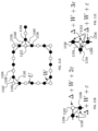
本開示のいくつかの局面は、プログラム可能なアレイにキュービットを配置するための系および方法に関し、該キュービットは、効率的な方法でより広い組の最適化問題をエンコードするかまたは近似的にエンコードし得る。いくつかの態様において、近接する「アンシラリー」キュービットの偶数の鎖は、例えば図2Aに関してより詳細に記載されるように、アンシラリーキュービットの鎖を用いて遠いキュービットを連結することにより、遠いキュービットの間の相互作用をエンコードするために使用される。本開示を通じてより詳細に記載されるように、「アンシラリー」キュービットのこれらの鎖は、他の頂点キュービットではなく特定の「頂点」キュービットの間の相互作用をエンコードするために使用され得、エッジにより連結されることを意図されない2つの頂点キュービットの間の長距離の相互作用の強さを低減するために使用され得る。いくつかの態様において、長距離の相互作用の効果は、特定のキュービットの間の相互作用を選択的に制御するために、離調パラメーターを選択された制御技術に導入することによりさらに低減され得る。例えば、コーナーおよびジャンクションキュービットについて、本開示に記載される離調パターンは、長距離の相互作用の効果を低減し得、その結果、系の基底状態は、エンコードされた問題に対する最適な解である。本明細書に記載される技術は、単純な単位円グラフを超えるより大きな組の最適化問題の効率的なエンコードを可能にし得る。 Some aspects of this disclosure relate to systems and methods for arranging qubits in programmable arrays that encode or approximate a broader set of optimization problems in an efficient manner. can be encoded to In some embodiments, even chains of adjacent "ancillary" qubits are formed by linking distant qubits with chains of ancillary qubits, for example, as described in more detail with respect to FIG. 2A. Used to encode interactions between distant qubits. As described in more detail throughout this disclosure, these chains of "ancillary" qubits can be used to encode interactions between specific "vertex" qubits rather than other vertex qubits. , can be used to reduce the strength of long-range interactions between two vertex qubits that are not intended to be connected by an edge. In some embodiments, the effects of long-range interactions are further reduced by introducing detuning parameters into selected control techniques to selectively control interactions between specific qubits. obtain. For example, for corner and junction qubits, the detuning patterns described in this disclosure can reduce the effects of long-range interactions, so that the ground state of the system is the optimal solution to the encoded problem. be. The techniques described herein may enable efficient encoding of larger sets of optimization problems beyond simple unit pie charts.

本開示のいくつかのさらなるまたは代替的な局面は、励起を含むキュービットの内部状態をコヒーレントに操作するための系および方法に関する。いくつかの態様において、エンコードされた問題を進展させ最適な(または近似的に最適な)解を見出すために使用され得る技術が、開示される。例えば、本開示の態様は、量子近似最適化アルゴリズム(「QAOA」)を実施するための最適変動性パラメーターおよび戦略に関し、そのうちいくつかの態様は、例えば、図14Aに関して記載される。例えば、態様は、古典的なフィードバックループのためのヒューリスティックを含み、これは、腕ずくのQAOA実行の性能を改善し得る。いくつかの態様において、これらの戦略は、現存するアルゴリズム以下である場合、少なくとも同様に実施される。本開示のいくつかの局面は、MaxCut組合せ問題を解くためにQAOAを使用する実行に焦点を合わせているが、開示された技術は、それに限定されない。 Some additional or alternative aspects of this disclosure relate to systems and methods for coherently manipulating qubit internal states, including excitations. In some aspects, techniques are disclosed that can be used to evolve an encoded problem and find an optimal (or nearly optimal) solution. For example, aspects of the present disclosure relate to optimal variability parameters and strategies for implementing a Quantum Approximation Optimization Algorithm (“QAOA”), some aspects of which are described, eg, with respect to FIG. 14A. For example, aspects include heuristics for classical feedback loops, which can improve the performance of brute force QAOA implementations. In some embodiments, these strategies are performed at least as well as if less than existing algorithms. Although some aspects of this disclosure focus on implementations using QAOA to solve the MaxCut combinatorial problem, the disclosed techniques are not so limited.

例示的な最適化問題およびエンコード
いくつかの態様において、特定の型の最適化問題は、キュービットの配置を用いてエンコードされ得る。例えば、図1A~1Eは、いくつかの態様によるキュービットのアレイを使用して最適化問題に対する解をエンコードするおよび見出すための例示的な図解を示す。図1Aは、いくつかの態様による単位円グラフ上のリュードベリブロッケード機構(Rydberg blockade mechanism)および最大独立集合の局面を示す。本開示に記載される技術を使用して解かれ得る1つの例示的な最適化問題は、最大独立集合(「MIS」)問題である。グラフGが頂点VおよびエッジEを有すると仮定すると、独立集合は、対がエッジにより連結されていない頂点のサブセットとして、画定され得る。図1Aは、102、104などの頂点を有する例示的なグラフを示す。頂点102、104は、エッジ106などのエッジを介して連結され得る。MIS問題のコンピューター的タスクは、最大独立集合(MIS)と呼ばれる最大のかかる集合を見出すことである。図1Aのグラフに示されるように、最大独立集合は、102などの黒の頂点を介して示され、これらのどれも連結されていない。図1Aの例において、最大独立集合のサイズは、6である。MISのサイズが任意のグラフGについての所定の整数aより大きいかどうかを決定することは、周知のNP-完全問題(NP-complete problem)である。さらに、MISのサイズを近似することでさえ、NP-困難問題(NP-hard problem)である。いくつかの態様において、MIS問題はまた、最大クリーク問題および最小頂点被覆問題と同等である。従って、MIS問題に対する解は、対応する最大クリーク問題および最小頂点被覆問題に対する解を構成する。
Exemplary Optimization Problems and Encodings In some aspects, certain types of optimization problems may be encoded using qubit arrangements. For example, FIGS. 1A-1E show exemplary diagrams for encoding and finding solutions to optimization problems using arrays of qubits according to some aspects. FIG. 1A shows aspects of the Rydberg blockade mechanism and maximum independent set on a unit pie chart according to some embodiments. One exemplary optimization problem that can be solved using the techniques described in this disclosure is the maximum independent set (“MIS”) problem. Suppose a graph G has vertices V and edges E, an independent set can be defined as the subset of vertices whose pairs are not connected by edges. FIG. 1A shows an exemplary graph with vertices 102, 104, and so on. Vertices 102 , 104 may be connected via edges, such as edge 106 . The computational task of the MIS problem is to find the largest such set, called the maximum independent set (MIS). As shown in the graph of FIG. 1A, maximal independent sets are indicated via black vertices such as 102, none of which are connected. In the example of FIG. 1A, the maximum independent set size is six. Determining whether the size of MIS is greater than a given integer a for any graph G is a well-known NP-complete problem. Moreover, even approximating the size of the MIS is an NP-hard problem. In some embodiments, the MIS problem is also equivalent to the maximum clique problem and the minimum vertex cover problem. The solution to the MIS problem thus constitutes the solution to the corresponding max clique and minimal vertex cover problems.

理論に拘束されることなく、図1Aの態様は、単位円(「UD」)グラフと言われ得る。UDグラフは、頂点が2D面に配置され、それらの対の距離が単位長rよりも小さい場合連結される幾何学的グラフである。換言すれば、UDグラフは、互いから距離r以内の任意の2つの頂点がエッジにより連結される、例えば、頂点102、104がエッジ106を介して連結されるグラフである。頂点108は、頂点102、104から遠すぎてエッジを用いてそれと連結できない。UDグラフ上のMIS問題(UD-MIS)は、なおNP-完全であり、種々の工業分野における例えば、ワイヤレスネットワーク設計からマップラべリング(map labelling)までにわたる実際の状況を見出すために使用され得る。 Without being bound by theory, the embodiment of FIG. 1A may be referred to as a unit circle (“UD”) graph. A UD graph is a geometric graph whose vertices are located in 2D faces and are connected if their pairwise distance is less than unit length r. In other words, a UD graph is a graph in which any two vertices within a distance r of each other are connected by an edge, eg vertices 102 , 104 are connected via edge 106 . Vertex 108 is too far from vertices 102, 104 to connect with it using an edge. The MIS problem on UD graphs (UD-MIS) is still NP-complete and can be used to find practical situations in various industrial fields ranging from e.g. wireless network design to map labelling. .

いくつかの態様において、MIS問題は、スピン-1/2と各頂点

Figure 0007287705000009
を結びつけることにより、エネルギー最小化問題として定式化され得る。図1Aに示されるもののような頂点は、経時的に変化するラビ周波数Ωおよび離調Δを有するもの(図1Dおよび1Eに示される)などの駆動シーケンスの後に、各キュービットの状態|1>がエネルギー的に好まれ、近くの頂点もまた状態|1>にある場合は別であり、この場合、1つの頂点が状態|0>に遷移することがエネルギー的に好まれるように調製され得る。理論に限定されることなく、かかる系のハミルトニアン(「HP」)は、以下のように表され得る:
Figure 0007287705000010
式中、スピン-1/2系は、状態|0>および|1>を各頂点に割り当て、nv=|1>υ<1|であり、Δは、スピン上の離調であり、Uは、エッジ(
Figure 0007287705000011
)により連結される2つのスピン(
Figure 0007287705000012
)の両方が状態|1>にある場合のエネルギーペナルティーである。最初に、全ての頂点を、|0>状態に調製し得る。駆動により、少なくともいくつかの頂点を|1>状態に遷移させる。Δ>0について、HPは、キュービットが状態
Figure 0007287705000013
にあることを好む。しかし、U>Δである場合、2つのキュービット、uおよびvが同時に状態
Figure 0007287705000014
にあることは、これらがエッジ
Figure 0007287705000015
により連結される場合、エネルギー的に好ましくない。従って、HPの各基底状態は、最大独立集合中の頂点に対応するキュービットが状態
Figure 0007287705000016
にあり、全ての他のキュービットが状態
Figure 0007287705000017
にある構成を示す。 In some embodiments, the MIS problem consists of spin-1/2 and each vertex
Figure 0007287705000009
can be formulated as an energy minimization problem by combining A vertex, such as the one shown in Fig. 1A, changes the state of each qubit after a driving sequence, such as the one with time-varying Rabi frequency Ω and detuning Δ (shown in Figs. 1D and 1E). is energetically favored and the nearby vertex is also in state |1>, in which case one vertex can be arranged so that it is energetically favored to transition to state |0> . Without being limited by theory, the Hamiltonian (“H p ”) of such a system can be expressed as follows:
Figure 0007287705000010
where the spin-1/2 system assigns states |0> and |1> to each vertex, n v =|1>ν<1|, Δ is the spin detuning, and U is the edge (
Figure 0007287705000011
) connected by two spins (
Figure 0007287705000012
) are both in state |1>. First, all vertices can be prepared to the |0> state. Driving causes at least some vertices to transition to the |1> state. For Δ>0, H P indicates that the qubit is in the state
Figure 0007287705000013
prefer to be in However, if U>Δ, then two qubits, u and v, are simultaneously in the state
Figure 0007287705000014
The thing is that these are the edges
Figure 0007287705000015
is energetically unfavorable when linked by Therefore, each ground state of HP is such that the qubit corresponding to the vertex in the maximally independent set is in the state
Figure 0007287705000016
with all other qubits in the state
Figure 0007287705000017
shows the configuration in .

図1Cは、いくつかの態様による弱い駆動Ω<<ΔおよびΔ>0の極限における2つの隣接する頂点の間の原子間相互作用ポテンシャルを示すグラフである。経時的に離調およびラビ周波数を変更することにより、系を初期状態から最終状態へと変更する量子進展が生じ得、該最終状態は、エンコードされた問題に対する解(または1つ以上の近似解)を含み得る。上記したように、かかる条件下では、rB(リュードベリブロッケード半径)よりも近いキュービットについて、キュービットの1つが|0>状態にとどまることがエネルギー的に好ましい。例えば、U>Δ>0である場合、ハミルトニアンHPは、スピンの対がエッジにより連結され(即ち、リュードベリ半径以内)ない限り、各スピンが状態|1(にあることをエネルギー的に好む。従って、ハミルトニアンHPの基底状態において、MIS中の頂点のみが、状態|1(にある。かかる状態は、MIS-状態と言われ得、HPは、MIS-ハミルトニアンと言われ得る。いくつかの態様において、MISのNP-完全決定問題は、HPの基底状態エネルギーが-αΔより低いかどうかを決定することになる。 FIG. 1C is a graph showing interatomic interaction potentials between two adjacent vertices in the limit of weakly driven Ω<<Δ and Δ>0 according to some embodiments. By changing the detuning and Rabi frequency over time, a quantum evolution can occur that changes the system from the initial state to the final state, which is the solution (or one or more approximate solutions) to the encoded problem. ). As noted above, under such conditions, for qubits closer than r B (the Ryde Veri-Bloccade radius), it is energetically favorable for one of the qubits to remain in the |0> state. For example, if U>Δ>0, the Hamiltonian HP energetically prefers each spin to be in state |1() unless the spin pair is connected by an edge (ie, within the Rydberg radius). Therefore, in the ground state of the Hamiltonian H P , only the vertices in MIS are in the state |1(. Such a state can be called the MIS-state, and H P can be called the MIS-Hamiltonian. In the embodiment of , the NP-complete decision problem of MIS becomes to determine whether the ground state energy of HP is lower than -αΔ.

いくつかの態様において、量子アニーリングアルゴリズム(「QAA」)は、初期状態から最終状態へと量子状態を進展させるために使用され得、該最終状態は、最適化問題に対する解をエンコードする。例えば、単純なQAAは、横磁場(transverse field)

Figure 0007287705000018
(式中、σx=|0><1|+|1><0|)を追加することにより実行され得、該横磁場は、異なるスピン配置間での量子トンネル現象(quantum tunneling)を誘導する。図1Bは、いくつかの態様によるスピン状態間の遷移を示す。例えば、ラビ周波数Ωと標識された矢印は、例えば、
Figure 0007287705000019
を有するレーザービームにより制御されるスピン状態|0>および|1>の間の遷移を記載する。離調Δ<0である場合、ハミルトニアンHPの基底状態は、全てのキュービットが|0>状態にあるトリビアルな状態である。離調Δ>0である場合、HPの基底状態は、状態|1>にあるキュービットがMISを形成するMIS状態である。例えば図1Eおよび1Dのそれぞれに示されるように時間依存的様式でΩおよびΔをゆっくり変更することにより、全てのキュービットが|0>にあるトリビアルな基底状態(Δ<0、Ω=0)は、MISをエンコードする最終状態(Δ>0、Ω=0)に断熱的に連結され得、キュービットは最適化問題に対する解に残る。一般的に、かかる手順は、本開示を通じてより詳細に議論されるように、消滅する(vanishing)エネルギーギャップにわたる遷移を含み得ることに留意のこと。シミュレーションの例示的かつ非限定的な態様は、表題「ランダムUD-MISのための量子アニーリング」の節により詳細に下記される。 In some embodiments, a quantum annealing algorithm (“QAA”) may be used to evolve quantum states from an initial state to a final state, which encodes the solution to the optimization problem. For example, a simple QAA uses the transverse field
Figure 0007287705000018
(where σ x =|0><1|+|1><0|), the transverse magnetic field induces quantum tunneling between different spin configurations do. FIG. 1B illustrates transitions between spin states according to some aspects. For example, the arrow labeled Rabi frequency Ω indicates, for example,
Figure 0007287705000019
We describe the transition between the spin states |0> and |1> controlled by a laser beam with For detuning Δ<0, the ground state of the Hamiltonian H P is the trivial state with all qubits in the |0> state. For detuning Δ>0, the ground state of HP is the MIS state where the qubits in state |1> form the MIS. For example, by slowly varying Ω and Δ in a time-dependent manner as shown in Figures 1E and 1D, respectively, the trivial ground state (Δ<0, Ω=0) with all qubits at |0> can be adiabatically linked to the final state (Δ>0, Ω=0) encoding the MIS, and the qubit remains the solution to the optimization problem. Note that in general such procedures may involve transitions across vanishing energy gaps, as will be discussed in more detail throughout this disclosure. Exemplary, non-limiting aspects of the simulation are described in more detail below in the section entitled "Quantum Annealing for Random UD-MIS."

いくつかの態様において、MIS問題は、個々の原子間のリュードベリ相互作用を使用して実行され得る。例えば、PCT/US18/42080により詳細に議論されるように、図1Aに示されるもののようなグラフは、2準位キュービットを使用して実行され得、該キュービットの状態は、いくつかの態様により図1Bに示される。光ピンセットを使用して、原子(キュービット)を、1次元、2次元および3次元でさえの十分にプログラム可能なアレイに個々にかつ決定論的に配置し得る。かかる系は、いわゆるリュードベリブロッケード機構を介して相互作用する個々に捕捉され均一に励起された中性原子を使用し得る。各原子は、内部基底状態|0>および高度に励起された長持ちするリュードベリ状態|1>を有するキュービット

Figure 0007287705000020
を実現し、これは、外部のレーザー場によりコヒーレントに操作され得る。2つの原子の両方がこのリュードベリ状態にあり、リュードベリブロッケード半径以内にある場合、該2つの原子は、強いファンデルワールス相互作用を介して相互作用し、これは、エネルギー的に好ましくない。これは、以下により詳細に説明するように、頂点としてキュービットを使用しリュードベリ半径により設定される円サイズを使用してUD-MIS問題をエンコードすることを可能にし得る。図9は、UD-MIS問題に対する例示的な解を示し、ここで、いくつかの態様により、いくつかのキュービット904は、内部基底状態|0>に見いだされ、他のキュービット902は、長持ちするリュードベリ状態|1>に見いだされる。 In some embodiments, the MIS problem can be performed using Rydberg interactions between individual atoms. For example, as discussed in more detail in PCT/US18/42080, graphs such as the one shown in FIG. An embodiment is shown in FIG. 1B. Using optical tweezers, atoms (qubits) can be individually and deterministically arranged into fully programmable arrays in one, two, and even three dimensions. Such systems may employ individually trapped and uniformly excited neutral atoms that interact through the so-called Rydberg blockade mechanism. Each atom is a qubit with an internal ground state |0> and a highly excited and long-lived Rydberg state |1>
Figure 0007287705000020
, which can be coherently manipulated by an external laser field. When two atoms are both in this Rydberg state and within the Rydberg blockade radius, the two atoms interact via strong van der Waals interactions, which are energetically unfavorable. This may allow encoding the UD-MIS problem using qubits as vertices and a circle size set by the Rydberg radius, as described in more detail below. FIG. 9 shows an exemplary solution to the UD-MIS problem, where some qubits 904 are found in the internal ground state |0> and other qubits 902 are found in the internal ground state |0> according to some aspects. It is found in the long-lasting Rydberg state |1>.

理論に限定されることなく、かかる系の態様の進展を支配するハミルトニアンは、以下のように表され得る:

Figure 0007287705000021
式中、
Figure 0007287705000022
は、キュービットvの位置
Figure 0007287705000023
でのラビ周波数およびレーザー離調である。個々の操作が可能であるが、かかる系はまた、例えば、
Figure 0007287705000024
である均一な駆動レーザーを用いて実行され得る。演算子
Figure 0007287705000025
は、キュービットvがリュードベリ状態にある場合に、キュービットvのコヒーレントなスピンフリップおよび
Figure 0007287705000026
計数(count)を生じ得る。いくつかの態様において、等方性リュードベリ状態について、原子間相互作用強度は、相対的原子距離xにのみ依存し、
Figure 0007287705000027
により与えられ、式中、Cは定数である。短い距離での強い相互作用は、図1Cに示されるように、2つのキュービットが、リュードベリブロッケード半径
Figure 0007287705000028
以内にある場合に、同時に状態|1>にあることをエネルギー的に妨げ、いくつかの態様によるいわゆるブロッケード機構を生じる。これは、リュードベリハミルトニアンHRydとUD-MIS問題に対する解の間の関連を提供し得る。換言すれば、リュードベリブロッケードは、リュードベリ半径(rB)以内の近接するキュービットをエネルギー的に好ましくするが、両方をリュードベリ状態|1>にはさせない。UDグラフにおいてと同様に、この構成のいくつかの態様において、キュービットは、リュードベリブロッケード半径より短い距離だけ分離された場合、両方が状態|1>に見出され得ない。 Without being limited by theory, the Hamiltonian governing the evolution of aspects of such systems can be expressed as follows:
Figure 0007287705000021
During the ceremony,
Figure 0007287705000022
is the position of the qubit v
Figure 0007287705000023
is the Rabi frequency and laser detuning at . Although individual manipulations are possible, such systems can also be used, for example,
Figure 0007287705000024
can be implemented with a uniform drive laser where . operator
Figure 0007287705000025
is a coherent spin flip of qubit v and
Figure 0007287705000026
A count can be produced. In some embodiments, for isotropic Rydberg states, the atomic interaction strength depends only on the relative atomic distance x,
Figure 0007287705000027
where C is a constant. A strong interaction at short distances can be seen in Fig. 1C, where the two qubits are separated from each other by the Ryde Veriblockade radius
Figure 0007287705000028
When within, it energetically prevents being in state |1> at the same time, giving rise to the so-called blockade mechanism according to some aspect. This may provide a link between the Rydberg Hamiltonian H Ryd and the solution to the UD-MIS problem. In other words, the Rydberg blockade makes neighboring qubits within the Rydberg radius (r B ) energetically favorable, but does not let them both be in the Rydberg state |1>. As in the UD graph, in some aspects of this construction, the qubits cannot both be found in state |1> if they are separated by a distance less than the Ryde Veri-Brockade radius.

MIS-ハミルトニアンHPは、古典的な極限Ωv=0において、リュードベリハミルトニアンHRydといくつかの特徴を共有する。いくつかの態様において、例えば、任意のグラフがHPに許容される場合、主な相違点は、対の相互作用の達成可能な連結性(connectivity)にある。リュードベリブロッケード機構に最も密接に関連する特別な限られた種類のグラフを考慮し得る。これらのいわゆる単位円(UD)グラフは、頂点が面における座標に割り当てられ得、単位距離r以内にある頂点の対のみがエッジにより連結される場合、上記されるように構築される。従って、単位距離rは、HRydにおけるリュードベリブロッケード半径rBと類似の役割を果たす。換言すれば、キュービットの空間的近接は、UD-MIS問題中のエッジをエンコードするために使用される。MISは、かかる単位円グラフに制限されている場合でさえ、NP-完全である。本開示の態様は2D問題およびキュービットの2D配置を議論するが、当業者は、本開示に基づいて、本明細書に記載される問題エンコードの局面が、1次元構造または3次元構造などの他の空間的構造に適用可能であることを理解する。 The MIS-Hamiltonian H P shares some features with the Rydberg Hamiltonian H Ryd in the classical limit Ω v =0. In some embodiments, for example, where arbitrary graphs are allowed in HP , the main difference lies in the achievable connectivity of pairwise interactions. A special limited class of graphs most closely related to the Ryde Veri blockade mechanism may be considered. These so-called unit circle (UD) graphs are constructed as described above, where vertices can be assigned coordinates on a face and only pairs of vertices within a unit distance r are connected by an edge. Thus, the unit distance r plays an analogous role to the Ryde Veri Blockade radius r B in H Ryd . In other words, the spatial proximity of qubits is used to encode edges in the UD-MIS problem. MIS is NP-complete even when restricted to such unit pie charts. Although aspects of the present disclosure discuss 2D problems and 2D arrangements of qubits, one of ordinary skill in the art, based on the present disclosure, will appreciate that aspects of the problem encoding described herein can be applied to structures such as one-dimensional or three-dimensional structures. Understand that it is applicable to other spatial structures.

理論に拘束されることなく、重み付き最大独立集合問題は、MIS問題であり、ここで、各頂点vが重み

Figure 0007287705000029
を有し、これは、等式1の同種の重みΔと置き換えたものである。重み付き最大独立集合問題は、最大の重みの合計和を有する独立集合を見出すことである。いくつかの態様実行において、これらの重み
Figure 0007287705000030
は、対応する光シフトを各キュービットに適用することにより、エンコードされ得る。いくつかの態様において、これらの光シフトは、共鳴から離れた(off-resonant)レーザービームまたは空間的光変調器により作製されるACシュタルクシフトであり得る。 Without being bound by theory, the weighted maximum independent set problem is the MIS problem, where each vertex v has a weight
Figure 0007287705000029
, which replaces the like weight Δ in Equation 1. The weighted maximal independent set problem is to find the independent set with the maximum total sum of weights. In some implementations, these weights
Figure 0007287705000030
can be encoded by applying a corresponding optical shift to each qubit. In some embodiments, these optical shifts can be AC Stark shifts produced by off-resonant laser beams or spatial light modulators.

例示的なキュービット配置および離調
リュードベリ相互作用は、リュードベリ半径を越えると有意に減衰するが、図1Aに示すように、102および108などの遠いキュービットの間になお長距離の相互作用テール(interaction tail)がある。相互作用テールは、単独でも集合でも、図1Dおよび1Eに示すものなどの駆動の後に、系が解にあることが見出される可能性を低減し得る。従って、図1Aに示すものなどの実行が、常に完璧にNP-完全MIS問題をエンコードするわけではない場合がある。さらに、図1Aに関して記載される技術を使用してエンコードされ得るNP-完全問題の範囲は、単位円に関連するものに限定される。
Exemplary qubit arrangements and detuning Although the Rydberg interaction significantly decays beyond the Rydberg radius, there are still long-range interaction tails between distant qubits such as 102 and 108, as shown in Fig. 1A. (interaction tail). Interaction tails, either alone or collectively, can reduce the likelihood that the system will be found in solution after a drive such as that shown in FIGS. 1D and 1E. Therefore, implementations such as the one shown in FIG. 1A may not always perfectly encode NP-complete MIS problems. Furthermore, the range of NP-complete problems that can be encoded using the techniques described with respect to FIG. 1A is limited to those related to the unit circle.

いくつかの態様において、これらの問題の1つ以上は、2次元における原子位置およびレーザーパラメーターを、リュードベリハミルトニアンHRydの低エネルギー領域が、最大次数3を有する平面グラフ上で(NP-完全)MIS-ハミルトニアンHPに単純化されるように、選択することにより解かれ得る。本開示のいくつかの局面において、反強磁性秩序は、リュードベリブロッケード機構のために、正の離調においてアンシラリーキュービットの(準)1Dスピン鎖の基底状態にあることが見出され得る。かかる構成は、ブロッケード束縛を遠い頂点キュービットの間で効果的に送り得る。本開示の他の局面において、離調パターン[Δv]は、基底状態スピン構成を変えることなく、所望されない長距離の相互作用の効果を排除するために導入され得る。いくつかの態様は、NP-完全問題の捕捉された中性原子のアレイの基底状態における効率的なエンコードを可能にする。理論に拘束されることなく、かかる態様における2Dアレイ中のリュードベリ相互作用原子の基底状態エネルギーは、NP-困難(およびΩv=0である場合、NP-完全)である。 In some embodiments, one or more of these problems solve the problem of determining atomic positions and laser parameters in two dimensions on a planar graph where the low-energy region of the Rydberg Hamiltonian H Ryd has maximal degree 3 (NP-complete) MIS -Hamiltonian can be solved by choosing to simplify to H P . In some aspects of the present disclosure, antiferromagnetic order can be found in the ground state of the (quasi) 1D spin chains of the ancillary qubits at positive detuning due to the Ryde Veriblockade mechanism. Such a configuration can effectively send blockade constraints between distant vertex qubits. In other aspects of the present disclosure, detuning patterns [Δ v ] can be introduced to eliminate the effects of undesired long-range interactions without changing the ground state spin configuration. Some embodiments enable efficient encoding in the ground state of arrays of trapped neutral atoms for NP-complete problems. Without being bound by theory, the ground state energies of Rydberg interacting atoms in 2D arrays in such embodiments are NP-hard (and NP-complete if Ω v =0).

アンシラリーキュービットを用いる例示的なキュービット配置
図2Aおよび2Bに関して記載されるように、NP-完全問題は、「頂点」キュービットの間でエッジを実行する(implement)「アンシラリー」キュービットまたは頂点を用いてエンコードされ得、ここで、いくつかの態様により、頂点キュービットは、3の最大次数を有する。例えば、図2Aに示されるように、複数の頂点キュービット202、204、212、214、および216は、グラフにおいて配置され得る。頂点キュービット202および204などの頂点キュービットの対の間のエッジは、偶数のアンシラリーキュービット206を使用して実行され得、それらの各々は、単位長rだけ分離される。この技術は、最大次数3を有する平面グリッドグラフをUDグラフに埋め込む(embed)ために使用され得る。例えば、最大次数3を有する平面グラフは、いくつかの態様により図2Aに示されるように、偶数のアンシラリー頂点を各エッジに沿って導入することにより、グリッド(グリッド単位gを有する)

Figure 0007287705000031
に効率的に埋め込まれ得、UDグラフGに変換され得る。UD半径
Figure 0007287705000032
は、各エッジに沿ったアンシラリー頂点の直線密度(linear density)に比例したパラメーターkにより決定され得る。いくつかの態様によると、各頂点を形成する相互作用がほぼ等しい強さであることを確実にするにするために、任意の所定のエッジに沿ってほぼ同じ密度のアンシラリーキュービットを実行することが望ましい。 Exemplary Qubit Arrangements Using Ancillary Qubits As described with respect to FIGS. 2A and 2B, the NP-complete problem is to implement an edge between the 'vertex' qubits, the 'ancillary' qubits or It can be encoded with vertices, where in accordance with some aspects the vertex qubits have a maximum degree of three. For example, as shown in FIG. 2A, multiple vertex qubits 202, 204, 212, 214, and 216 can be arranged in a graph. Edges between pairs of vertex qubits, such as vertex qubits 202 and 204, may be implemented using even ancillary qubits 206, each of which is separated by unit length r. This technique can be used to embed a planar grid graph with maximum degree 3 into a UD graph. For example, a planar graph with maximum degree 3 can be gridded (with grid unit g) by introducing an even number of ancillary vertices along each edge, as shown in FIG. 2A according to some aspects.
Figure 0007287705000031
can be efficiently embedded in and converted to the UD graph G. UD radius
Figure 0007287705000032
can be determined by a parameter k proportional to the linear density of the ancillary vertices along each edge. According to some aspects, we run approximately the same density of ancillary qubits along any given edge to ensure that the interactions forming each vertex are of approximately equal strength. is desirable.

頂点キュービット202および204の例において、頂点キュービット202は、最も左のアンシラリーキュービット206と、まるでそれが頂点キュービット204であるかのように相互作用し得、頂点キュービット204は、最も右のアンシラリーキュービット206と、まるでそれが頂点キュービット202であるかのように相互作用し得る。この様式において、エッジは、リュードベリ半径の外側の頂点キュービットの間でかつ単位円グラフとして純粋に実行できない様式で実行され得る。さらに、図1Aに関して議論したもののような単位円グラフにおいて、いくつかの頂点をエッジにより連結される同じ距離だけ分離させ(例えば、頂点キュービット202、204)、一方で、同じ距離だけ分離される他の頂点をエッジにより連結しない(例えば、頂点キュービット212、214)ことは可能ではないが、かかる構成は、本開示に記載されるアンシラリー頂点を使用して実現され得る。 In the example of vertex qubits 202 and 204, vertex qubit 202 can interact with leftmost ancillary qubit 206 as if it were vertex qubit 204, and vertex qubit 204 can: It can interact with the rightmost ancillary qubit 206 as if it were the vertex qubit 202 . In this fashion, edges can be implemented between vertex qubits outside the Rydberg radius and in a manner not purely feasible as a unit pie graph. Further, in a unit pie graph such as the one discussed with respect to FIG. 1A, some vertices are separated by the same distance connected by edges (e.g., vertex qubits 202, 204) while separated by the same distance. While it is not possible to have other vertices not connected by edges (eg, vertex qubits 212, 214), such configurations can be achieved using the ancillary vertices described in this disclosure.

例示的な離調パターン
いくつかの態様において、MISグラフが図2Aに示されるように実行される場合、リュードベリ相互作用のテールは、コーナーおよびジャンクションの近傍を除いて、キュービット間の相互作用に影響を及ぼさず、そこでは、アンシラリーキュービットのアレイは、ある角度をなす。頂点キュービット202は、例示的なコーナーであり、頂点キュービット216は、例示的なジャンクションである。図2Bに関してより詳細に記載されるように、キュービットの駆動の間の離調パターンは、相互作用テールの効果を相殺するために、これらの構造の周りで調整され得る。
Exemplary Detuning Patterns In some embodiments, if the MIS graph is performed as shown in FIG. No effect, where the array of ancillary qubits is at an angle. Vertex qubit 202 is an exemplary corner and vertex qubit 216 is an exemplary junction. As described in more detail with respect to FIG. 2B, the detuning pattern during qubit actuation can be tuned around these structures to counteract the effects of interaction tails.

図2Bは、いくつかの態様によるかかる離調パターンの例を示す。図2Bの挿入図は、図2A中の頂点キュービット216などの3の次数を有する頂点キュービット216を示し、これは、第1の方向において、近接するアンシラリーキュービット222、224であり、第2の方向において、232、234であり、第3の方向において、242、244である。図2Bは、垂直(水平)方向に沿って離調Δcを有する頂点キュービットから距離jにあるキュービットの離調

Figure 0007287705000033
をプロットする。図2Bに示されるように、離調
Figure 0007287705000034
は、各アンシラリーキュービット(例えば、PCT/US18/42080に記載される個々のアドレシング(addressing)技術を使用して)個々にアドレシングされ得、相互作用テールの効果を排除する様式で設定され得る。例えば、離調
Figure 0007287705000035
は、範囲
Figure 0007287705000036
かつ十分に大きなkで選択され得る。いくつかの態様において、離調は、この範囲内で任意に選択され得る。かかる離調は、長距離の相互作用の所望されない効果を相殺し得る。かかる条件下では、HRydの基底状態において(Ωv=0で)、アンシラリーキュービットの各アレイは、|0>と|1>の間で交替する(せいぜい1つのドメイン壁を有する)秩序だった構成にある。これは、Ωv=0についてのHRyd(2)の基底状態が、Gに対するMISハミルトニアン(1)の基底状態と同時に生じることを確実にする。個々のアンシラリーキュービットについての離調のこの摂動は、全体的な(global)駆動パターンの複数の異なる型(本開示を通じてより詳細に記載されるQAAおよびQAOAなど)を用いて、MISに対する解が何であるかの前もっての知識なしに、実施され得る。さらに、G上のMISのサイズは、アンシラリー頂点の数の半分まで、
Figure 0007287705000037
上のMISのサイズと同一であるので、MIS問題がアンシラリー頂点を使用して実行される場合、リュードベリハミルトニアン(2)の基底状態を見出すことはなおNP-困難である。 FIG. 2B shows examples of such detuning patterns according to some aspects. The inset of FIG. 2B shows a vertex qubit 216 with degree 3, such as the vertex qubit 216 in FIG. 232, 234 in the second direction and 242, 244 in the third direction. Figure 2B shows the detuning of a qubit at distance j from the vertex qubit with detuning Δc along the vertical (horizontal) direction.
Figure 0007287705000033
to plot Detuning as shown in Figure 2B
Figure 0007287705000034
can be individually addressed (e.g., using individual addressing techniques described in PCT/US18/42080) and set in a manner that eliminates the effects of interaction tails . For example, detuning
Figure 0007287705000035
is the range
Figure 0007287705000036
and can be selected with a sufficiently large k. In some embodiments, the detuning can be chosen arbitrarily within this range. Such detuning can offset the undesirable effects of long-range interactions. Under such conditions, in the ground state of H Ryd (at Ω v =0), each array of ancillary qubits is ordered (with at most one domain wall) alternating between |0> and |1> was in the configuration. This ensures that the ground state of H Ryd (2) for Ω v =0 occurs simultaneously with the ground state of the MIS Hamiltonian (1) for G. This perturbation of detuning for individual ancillary qubits provides solutions to MIS using multiple different types of global drive patterns (such as QAA and QAOA, which are described in more detail throughout this disclosure). can be implemented without prior knowledge of what Moreover, the size of the MIS on G is up to half the number of ancillary vertices,
Figure 0007287705000037
Identical to the size of the MIS above, it is still NP-hard to find the ground state of the Rydberg Hamiltonian (2) if the MIS problem is performed using ancillary vertices.

いくつかの態様において、実行は、単位円グラフを超えて、より一般的なグラフまで拡張され得る。かかる実行は、「ストロボ的」実行と言われ得、これは、図2Aに関して記載されるアンシラリーキュービットを用いずに実行される任意のグラフを含み得る。例えば、いくつかの態様において、種々の光学的技術が、これらの系にアドレシングされ得る問題の種類を拡張するために使用され得る。1つの例示的なアプローチは、キュービットを基底-リュードベリキュービットエンコードではなく超微細基底状態(hyperfine ground state)にエンコードすること、およびリュードベリSおよびP状態などの種々の種類をリュードベリ状態へと選択的に励起すること(例えば、キュービットの個々のアドレシングを用いて)を含む。この例において、異なるパリティーSおよびPを有するリュードベリ状態間の強く長距離の双極性相互作用は、その複数の隣接体(neighbor)により制御される単一キュービットの回転を効率的に実現するために使用され得る。例えば、リュードベリSおよびP状態は、多キュービット-制御回転を実現するために使用され得る。回転(またはキュービットフリップ)は、量子状態を初期状態から最終MIS-状態に進展させるために使用され得る。これらの相互作用を制御することにより、例えば、2つのキュービットが、エッジにより連結される場合に、両方ともリュードベリ状態にあるように進展しないことを確実にすることにより、系の進展が独立集合の束縛を破らないことを確実にすることが可能である。いくつかの例において、所定の(中央)キュービットの全ての隣接体は、状態

Figure 0007287705000038
からS-状態に選択的に励起され得る。その後、中央キュービットの2つの超微細状態の間とリュードベリP-状態における中間段階との2段階遷移は、多キュービット-制御回転を実行し得る。トロタライズド(Trotterized)時間進展(例えば、全ハミルトニアン進展を小さな不連続な段階に分割すること)と合わせると、これらの技術は、UDグラフを超えるための手段を提供し、任意のグラフ上のMIS問題に対する種々の量子最適化アルゴリズムを実行する。いくつかの態様において、この技術は、図2Aに描かれるものよりも広い範囲のグラフを含み得る任意のグラフを実行し得る。いくつかの態様において、「ストロボ的実行」(キュービットのリュードベリ状態への選択的かつ連続的な励起)は、多キュービット-制御回転の実行を可能にする。この選択的な励起は、グラフ構造に従った制御された回転を容易にし得、該グラフ構造は、単位円幾何構造に必ずしも限定されない。 In some aspects, implementations can be extended beyond unit pie charts to more general charts. Such an execution may be referred to as a "stroboscopic" execution, which may include any graph executed without the ancillary qubits described with respect to FIG. 2A. For example, in some embodiments various optical techniques can be used to expand the types of problems that can be addressed with these systems. One exemplary approach is to encode the qubits into a hyperfine ground state rather than a basis-Rydberg qubit encoding, and select different kinds of Rydberg S and P states into the Rydberg state. excitation (eg, using individual addressing of the qubits). In this example, the strong, long-range bipolar interactions between Rydberg states with different parities S and P allow efficient rotation of a single qubit controlled by its multiple neighbors. can be used for For example, Rydberg S and P states can be used to realize multi-qubit-controlled rotations. A rotation (or qubit flip) can be used to evolve the quantum state from the initial state to the final MIS-state. By controlling these interactions, for example, by ensuring that two qubits, when connected by an edge, do not evolve such that they are both in the Rydberg state, the evolution of the system is independent set It is possible to ensure that the bindings of In some examples, all neighbors of a given (central) qubit are state
Figure 0007287705000038
can be selectively excited from to the S-state. A two-step transition between the two hyperfine states of the central qubit and an intermediate step in the Rydberg P-state can then perform a multi-qubit-controlled rotation. Combined with Trotterized time evolution (e.g., dividing the total Hamiltonian evolution into small discrete steps), these techniques provide a means to go beyond the UD graph and solve the MIS problem on arbitrary graphs. perform various quantum optimization algorithms on . In some embodiments, this technique may implement any graph that may include a broader range of graphs than that depicted in FIG. 2A. In some embodiments, "stroboscopic execution" (selective and sequential excitation of qubits into Rydberg states) enables the execution of multi-qubit-controlled rotations. This selective excitation may facilitate controlled rotation according to a graph structure, which is not necessarily limited to the unit circle geometry.

例示的な古典的および量子アルゴリズムの比較
いくつかの態様によると、量子コンピューター計算を用いて解を見出すことが標準的なコンピューター計算アプローチに対して大きな改善を示すUD-MIS問題の型を同定することが望ましい。古典的および量子アルゴリズムの両方の数値的シミュレーションは、量子アルゴリズムがUD-MISに十分に適合する型(regime)および系サイズを同定するために使用され得る。1つの態様において、N個の頂点を、ランダムに密度ρで、サイズL×Lの2Dボックス(ここで、

Figure 0007287705000039
およびUD半径r=1)中に配置することにより構築されるランダムUDグラフ上のMISが考察され得る。この問題の困難さは、頂点密度に依存し得る:密度が、浸透閾域(percolation threshold)
Figure 0007287705000040
未満である場合、グラフは、連結されない有限のクラスターに分解され、効率的な多項式時間アルゴリズム(polynomial time algorithm)を可能にする。反対の極限において、例えば、密度が非常に大きい、
Figure 0007287705000041
である場合、問題は、既知の最良のパッキング比が
Figure 0007287705000042
である(連続的な)2D面における円の最密充填(closest packing)に本質的になる。 Comparison of Exemplary Classical and Quantum Algorithms According to some embodiments, we identify types of UD-MIS problems for which finding solutions using quantum computation represents a significant improvement over standard computational approaches. is desirable. Numerical simulations of both classical and quantum algorithms can be used to identify regimes and system sizes for which quantum algorithms are well suited for UD-MIS. In one embodiment, N vertices are randomly placed with density ρ in a 2D box of size L×L (where
Figure 0007287705000039
and the MIS on a random UD graph constructed by placing in the UD radius r=1). The difficulty of this problem may depend on the vertex density:
Figure 0007287705000040
If less than, the graph is decomposed into finite unconnected clusters, allowing an efficient polynomial time algorithm. In the opposite limit, e.g., the density is very large,
Figure 0007287705000041
, the problem is that the best known packing ratio is
Figure 0007287705000042
is essentially the closest packing of circles in a (continuous) 2D surface where .

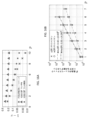
図3A~3Bは、いくつかの態様による例示的な古典的な最適化アルゴリズムの性能を示す。特に、それは、いくつかの密度領域において、古典的なアルゴリズムが最適化問題を解くことが困難であり、正確に解くために指数関数的な時間を必要とすることを示す。これらの型において、量子利点(quantum advantage)は、他の型よりも有益である。図4A~4Dは、いくつかの態様による量子アルゴリズム(QAAおよびQAOAの両方)の対応する性能を示す。スモール-サイズシミュレーションを用いた実行によると、図4A~4Dは、QAOAが問題を迅速に解き得、QAAに勝り得ることを示す。図4A~4Dは、いくつかの態様による特定の型についての量子利点を示す。より具体的には、図3Aは、古典的な最適化アルゴリズムの性能を示すグラフであり、いくつかの態様による分岐限定アルゴリズムに焦点を合わせている。CPU時間においてMISを見出すためのメジアン運転時間Trunは、所定の数(垂直軸)および密度(水平軸)でビン(bin)について示される。図3Aに示される例示的な統計は、データ点あたり50のグラフから得られた。破線は、上記した浸透閾域を示し、これは、この場合において、

Figure 0007287705000043
であることが示される。図3Aに見られ得るように、Nおよびρのパラメーター空間の特定の型において、問題は、例えば、運転時間が大きいので、古典的な最適化アルゴリズムが解くのは困難である。 Figures 3A-3B illustrate the performance of an exemplary classical optimization algorithm according to some aspects. In particular, it shows that in some density regions classical algorithms have difficulty solving the optimization problem, requiring exponential time to solve it accurately. In these types the quantum advantage is more beneficial than in other types. 4A-4D show corresponding performance of quantum algorithms (both QAA and QAOA) according to some embodiments. According to an implementation using small-size simulations, FIGS. 4A-4D show that QAOA can solve the problem quickly and outperform QAA. Figures 4A-4D illustrate quantum advantages for particular molds according to some embodiments. More specifically, FIG. 3A is a graph showing the performance of classical optimization algorithms, focusing on branch and bound algorithms according to some aspects. The median run time T run to find the MIS in CPU time is shown for bins with a given number (vertical axis) and density (horizontal axis). The exemplary statistics shown in Figure 3A were obtained from 50 graphs per data point. The dashed line indicates the permeation threshold zone mentioned above, which in this case is
Figure 0007287705000043
is shown to be As can be seen in FIG. 3A, in certain types of N and ρ parameter spaces, the problem is difficult for classical optimization algorithms to solve, eg, because the run time is large.

図3Bは、いくつかの態様によるNの関数として運転時間Trunを示すグラフである。

Figure 0007287705000044
について多項式スケーリング(polynomial scaling)があるが、中間密度ρ~7において、運転時間は、N~150頂点を超えると、系サイズと指数関数的な依存性を示す。この指数関数的な依存性は、任意の所定の数Nについて最悪の場合および典型的な例の両方において見られ得る。ρ~7において、古典的なアルゴリズムは、しばしば、Odysseyコンピューター計算クラスター(ハーバード大学により運営される)の単一のノード(node)において、24時間のCPU時間以内に
Figure 0007287705000045
について解を見出すことができなかったことに留意のこと。より一般的な非-UDグラフについて、古典的なアルゴリズムのこの制限は、
Figure 0007287705000046
で観察される。比較のために、エッジ確率p=0.05を有するErdoes-Renyiグラフに対する性能もまた示され、類似した指数関数的な運転時間を示す。エラーバーは、100のグラフの中の5番目および95番目の百分位数値である。図3Bは、古典的なアルゴリズムが特定のサイズ(例えば、~N=400)の問題を解くのに長時間 (例えば、24時間)かかり得ることを示す。これは、問題が古典的に解くにはトリビアルではないように、問題サイズを試験量子アルゴリズムに通知する。 FIG. 3B is a graph showing run time T run as a function of N, according to some aspects.
Figure 0007287705000044
Although there is a polynomial scaling for , at intermediate densities ρ˜7, the run times show an exponential dependence with the system size beyond N˜150 vertices. This exponential dependence can be seen in both the worst case and typical cases for any given number N. At ρ~7, classical algorithms often run within 24 hours of CPU time on a single node of the Odyssey computing cluster (run by Harvard University).
Figure 0007287705000045
Note that we were unable to find a solution for For more general non-UD graphs, this limitation of classical algorithms is
Figure 0007287705000046
observed in For comparison, the performance for the Erdoes-Renyi graph with edge probability p=0.05 is also shown, showing similar exponential drive times. Error bars are 5th and 95th percentile values in 100 graphs. FIG. 3B shows that the classical algorithm can take a long time (eg, 24 hours) to solve a problem of a certain size (eg, ˜N=400). This informs the test quantum algorithm of the problem size so that the problem is not trivial to solve classically.

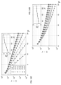
図4Aおよび4Bは、いくつかの態様によるランダムUDグラフ上のMISに対する量子アルゴリズムの性能を示すグラフである。図4Aは、いくつかの態様による断熱的時間スケールTLZに関する量子断熱的アルゴリズムについての困難さの図であり、垂直軸上のNに対して水平軸上に密度ρをプロットしている。例えば、図4Aは、上記したMISアニーリングハミルトニアンHD+HPを用い、

Figure 0007287705000047
としてパラメーターを掃引(sweep)した断熱的QAAの数値的シミュレーションの結果を示す。 4A and 4B are graphs illustrating performance of quantum algorithms for MIS on random UD graphs according to some embodiments. FIG. 4A is a difficulty diagram for the quantum adiabatic algorithm for the adiabatic time scale T LZ according to some embodiments, plotting density ρ on the horizontal axis against N on the vertical axis. For example, FIG. 4A uses the MIS annealing Hamiltonian H D +H P described above,
Figure 0007287705000047
The results of numerical simulations of adiabatic QAA with parameters swept as are shown.

極限

Figure 0007287705000048
が観察され得、そこでは、動力学が独立集合部分空間に限られ、系サイズN~40キュービットまでの数値的シミュレーションを可能にする。縞パターンに平行な傾斜した破線は、最適な円パッキングに対応する。十分に連結された領域は、トリビアルに
Figure 0007287705000049
を有する。断熱性に必要とされるLandau-Zener時間スケールTLZは、数値的結果を、基底状態確率
Figure 0007287705000050
の予想される長時間挙動にフィッティングすることにより抽出され得る。例えば、大きなTについてPMISをフィッティングさせTLZを抽出することが可能である。図4Aは、浸透閾域ρ=1.436での、問題を解くのに容易な型からそうではない型までの明確な遷移を示す。高い密度で、MISのサイズは、最適パッキング問題に対する関係のために、
Figure 0007287705000051
により決定され得る。これは、また、図4A中の縞パターンにより見られ得るTLZに反映される。指数関数的なヒルベルト空間サイズは、数値的シミュレーションを制限し、古典的なアルゴリズムのスケーリングとの決定的な比較を困難を超えるものにする。いくつかの実行において、有限のコヒーレンス時間は、量子断熱的経路に沿った基底状態と第1励起状態の間のエネルギーギャップに対応する最小エネルギーギャップ
Figure 0007287705000052
の指数関数的なスケーリングを伴う断熱的アルゴリズムの性能をさらに制限し得る。 limit
Figure 0007287705000048
can be observed, where the dynamics are confined to independent set subspaces, allowing numerical simulations up to system size N~40 qubits. Sloping dashed lines parallel to the fringe pattern correspond to optimal circle packing. Well-connected regions are trivially
Figure 0007287705000049
have The Landau-Zener timescale T LZ required for adiabaticity expresses the numerical results in terms of the ground state probabilities
Figure 0007287705000050
can be extracted by fitting to the expected long-term behavior of For example, it is possible to fit P MIS for large T and extract TLZ . FIG. 4A shows a clear transition from easy to not easy to solve problems with a penetration threshold ρ=1.436. At high densities, the size of the MIS is
Figure 0007287705000051
can be determined by This is also reflected in the TLZ , which can be seen by the fringe pattern in FIG. 4A. The exponential Hilbert space size limits numerical simulations and makes definitive comparisons with scaling of classical algorithms beyond difficult. In some implementations, the finite coherence time is the minimum energy gap corresponding to the energy gap between the ground state and the first excited state along the quantum adiabatic path
Figure 0007287705000052
can further limit the performance of adiabatic algorithms with exponential scaling of .

いくつかのアプローチが、これらの潜在的な制限の克服を試みるために実行され得る。かかるアプローチは、ギャップを利用できるようにする(open up)ためのヒューリスティックス、QAAにおける非断熱(diabatic)(非断熱的)遷移の使用、および下記で検討されるQAOAなどの変動性量子アルゴリズムを含む。図4Bは、いくつかの態様によるシミュレートされた非断熱的QAAについてのPMISであるMISを見出す確率を示すグラフである。いくつかの態様において、TLZおよびPMISは、類似した情報を運び得、大きなT(断熱的な型において)について、

Figure 0007287705000053
により関係付けられる。図4Aは、例示的な断熱的な型(大きなT)を示し、図4Bは、例示的な非断熱的な型(短いT)を示す。例えば、図4Bは、単一のTについての単一掃引(図4Aに示されるように、合計時間Tについての複数回の掃引ではない)を示し、これは、短いアニーリング時間
Figure 0007287705000054
での等式(Eq.)(3)におけるプロフィール(profile)を有する例示的な短時間極限(例えば、非断熱的)である。図4Bは、MIS状態との実質的な重複が、進展時間
Figure 0007287705000055
で得られ得、成功確率は、断熱的困難さの図に定性的に類似することを示す。これらの結果は、非断熱的アニーリングが、特に、最小スペクトルギャップ
Figure 0007287705000056
が小さい場合に有利であり得るという観察と一致する。いくつかの態様において、ギャップが小さい場合(他のエネルギースケールと比べて)、量子断熱的アルゴリズムを走らせるために長いコヒーレンス時間(例えば、
Figure 0007287705000057
)が必要とされ得る。 Several approaches can be implemented to attempt to overcome these potential limitations. Such approaches include heuristics to open up gaps, the use of diabatic (non-adiabatic) transitions in QAA, and fluctuating quantum algorithms such as QAOA, discussed below. . FIG. 4B is a graph showing the probability of finding a MIS that is a P MIS for simulated non-adiabatic QAA according to some embodiments. In some embodiments, T LZ and P MIS may carry similar information, and for large T (in adiabatic form)
Figure 0007287705000053
related by FIG. 4A shows an exemplary adiabatic mold (large T) and FIG. 4B shows an exemplary non-adiabatic mold (short T). For example, FIG. 4B shows a single sweep for a single T (rather than multiple sweeps for a total time T as shown in FIG. 4A), which has a short annealing time.
Figure 0007287705000054
is an exemplary short-time limit (eg, non-adiabatic) with the profile in (3). Figure 4B shows that the substantial overlap with the MIS state is
Figure 0007287705000055
, indicating that the probability of success is qualitatively similar to the adiabatic difficulty diagram. These results indicate that non-adiabatic annealing, especially the minimum spectral gap
Figure 0007287705000056
This is consistent with the observation that it may be advantageous if . In some embodiments, when the gap is small (relative to other energy scales), a long coherence time (e.g.,
Figure 0007287705000057
) may be required.

本開示を通じて記載されるように、ファンデルワールス相互作用を介して相互作用するスピンの多体問題とコンピューター的複雑性理論の直接の関連を利用することが可能である。かかるスピンの位置に対する個々の制御により、NP-完全最適化問題がかかる量子系に直接エンコードされる。この結果は、3の最大次数を有する平面グラフ上のMISからの簡略化から得られ得る。中性原子を捕捉および操作するための技術と組み合わせての本開示に記載される技術に基づく量子オプティマイザー(quantum optimizers)は、NP-困難な最適化問題を、従来のコンピューター計算技術に対する改善として扱い得る。 As described throughout this disclosure, it is possible to take advantage of the direct link between the spin many-body problem and computational complexity theory that interact via van der Waals interactions. Individual control over the position of such spins directly encodes the NP-perfect optimization problem into such quantum systems. This result can be obtained from a simplification from MIS on a planar graph with a maximum degree of 3. Quantum optimizers based on the techniques described in this disclosure in combination with techniques for trapping and manipulating neutral atoms solve NP-hard optimization problems as an improvement over conventional computational techniques. can handle.

例示的な量子アルゴリズム
上記で議論したように、上記した「アンシラリー」キュービット技術を使用しようとしまいといずれにせよ、量子系の位置を使用して組合せ問題をエンコードした後、次の段階は、組合せ問題に対する解である基底状態を生成する様式で、系を進展させることである。いくつかの例は、QAAおよびQAOAを含む。
Exemplary Quantum Algorithms As discussed above, whether or not the "ancillary" qubit technique described above is used, after encoding the combinatorial problem using the position of the quantum system, the next step is to: It is the evolution of the system in a manner that produces a ground state that is the solution to the combinatorial problem. Some examples include QAA and QAOA.

QAOA
いくつかの態様において、QAOAは、本開示に記載されるもののような量子最適化問題に適用され得る。例えば、(レベルpの)QAOAは、p共鳴パルスのシーケンスを、最初に調製される状態における異なる(varying)持続時間tkおよび光学的位相φkの全てのキュービット(または本開示により詳細に記載されるように、特定のキュービットに対するいくつかの離調およびエネルギー調整を有する)に適用することからなり得る。これは、変動性波動関数

Figure 0007287705000058
を生じ得る。理論に拘束されることなく、本開示は、いくつかのさらなるまたは代替的な最適化パラメーター(γ, β)を記載し、これは、いくつかの態様において、以下の表題MISに対するQAOAの節により詳細に記載されるように、持続時間tkおよび光学的位相φkに関連し得る。 QAOA
In some embodiments, QAOA may be applied to quantum optimization problems such as those described in this disclosure. For example, a (level p) QAOA can generate a sequence of p resonance pulses for all qubits (or as described, with some detuning and energy adjustments to a particular qubit). This is the fluctuating wavefunction
Figure 0007287705000058
can occur. Without being bound by theory, this disclosure describes several additional or alternative optimization parameters (γ, β), which in some embodiments are defined by the QAOA section for MIS below. As will be described in detail, it can be related to duration t k and optical phase φ k .

得られた量子状態は、コンピューターベースで測定され得、次いで、最適化に使用され得る。例えば、変動性パラメーターtkおよびφkは、この量子状態における

Figure 0007287705000059
の測定からの古典的なフィードバックループにおいて最適化され得る。この最適化の例は、以下により詳細に記載される。 The resulting quantum states can be computer-based measured and then used for optimization. For example, the variability parameters t k and φ k in this quantum state are
Figure 0007287705000059
can be optimized in a classical feedback loop from the measurement of Examples of this optimization are described in more detail below.

QAOAの性能は、選択された古典的な最適化ルーチンに一部依存する。かかる技術の例示的な実行を説明する前に、いくつかの態様において、古典的なコンピューター計算技術に対する改善を示すQAOAの性能を示し得る。例えば、図4Cは、例示的なグラフの例G0(N=32および独立集合空間次元dimIS=17734、ρ=2.4および

Figure 0007287705000060
)において、最適化QAOAと量子 アニーリングを比較し、該例について、いくつかの態様によると、断熱的時間スケールは、およそ
Figure 0007287705000061
であると観測され得る。図4Cに示されるように、QAOAは、デプス(depth)
Figure 0007287705000062
(即ち、40未満の共鳴パルス)でO(1)成功確率を達成し、それにより、有意により短い進展時間
Figure 0007287705000063
を示し、例外的に良好な変動性状態を示し、これは、アルゴリズムがエンコードされた問題を解くのに効果的であることを示し得る。そして、以下でより詳細に議論されるが、これは、また、大きな系に対するQAOAの実行に反映される。しかし、通常の数値解析(numerical analytics)を使用して評価され得る例示的な系サイズについて、測定射影ノイズと関連する変動は、MISサイズが、より小さなpであっても、古典的な最適化ルーチンの間に容易に見出され得ることを意味し得る。いくつかの態様において、この「測定射影ノイズ」は、測定中のノイズではない。例えば、各測定は、コンフィギュレーション空間(configuration space)を生じ得る。オブザーバブルの期待値を評価し、QAOA最適化を実施するために、測定は、複数回繰り返される必要がある。小さな系サイズについて、測定結果は、多くの最適化の前にMISをヒット(hit)し得、なぜなら、各測定はMISを生じる高い確率を有するからである。 The performance of QAOA depends in part on the classical optimization routine chosen. Before describing exemplary implementations of such techniques, in some embodiments, we can demonstrate the performance of QAOA, which represents an improvement over classical computational techniques. For example, FIG. 4C shows an illustrative graph example G 0 (N=32 and independent set spatial dimension dim IS =17734, ρ=2.4 and
Figure 0007287705000060
), comparing optimized QAOA with quantum annealing, and for the example, according to some embodiments, the adiabatic timescale is approximately
Figure 0007287705000061
It can be observed that As shown in Figure 4C, the QAOA is a depth
Figure 0007287705000062
(i.e., less than 40 resonant pulses) to achieve O(1) success probability, resulting in significantly shorter evolution times
Figure 0007287705000063
, indicating exceptionally good variability conditions, which may indicate that the algorithm is effective in solving the encoded problem. And, as discussed in more detail below, this is also reflected in the performance of QAOA on large systems. However, for an exemplary system size that can be evaluated using routine numerical analytics, the variation associated with measurement projection noise is less than that of classical optimization, even for smaller p for MIS size. It can mean that it can be easily found during the routine. In some embodiments, this "measurement projection noise" is not the noise in the measurement. For example, each measurement can yield a configuration space. Measurements need to be repeated multiple times to evaluate the expected value of observables and perform QAOA optimization. For small system sizes, measurements can hit the MIS before many optimizations, because each measurement has a high probability of producing an MIS.

図4Dは、いくつかの態様によるグラフG0に対する種々の量子アルゴリズムのシミュレートされた性能を示す。例えば、図4Dは、G0に対するシミュレートされたQAOAおよびQAAについてのM測定後に見出された真のMISと最大の独立集合の間の平均差を示す。図4Dに示されるように、ヒューリスティックアンサツ(ansatz)法およびランダム推測法を用いたQAOAの両方を示す。かかる結果を得るために、QAOAについてのシミュレーションを、射影測定からのサンプリングを含むモンテカルロシミュレーション技術を用いて実施した。最大の測定された独立集合のサイズを、測定数の関数としてプロットする(モンテカルロ軌跡(trajectory)にわたって平均した)。tkおよびφkについてヒューリスティック アンサツを適切に選択することにより、QAOA(p=3で)により、~102~103測定後に既にMISが見出される。これは、古典的な最適化ルーチンの一部として、

Figure 0007287705000064
を正確に評価するために必要な測定数と同等である。この性能は、非断熱的アニーリング時間T=1/Ω0、10/Ω0、100/Ω0について上記等式3により記載される掃引(およびΔ00=6)を用いたQAAの繰り返しのラン(run)と比較され得る。この小さな系サイズについて、QAOAは、アニーリング時間T~10/Ω0での非断熱的QAAとして同様に実施される。 FIG. 4D shows simulated performance of various quantum algorithms for graph G 0 according to some aspects. For example, FIG. 4D shows the average difference between the true MIS and the largest independent set found after M measurements for simulated QAOA and QAA for G 0 . As shown in Figure 4D, both QAOA using heuristic ansatz and random guessing methods are shown. To obtain these results, simulations for QAOA were performed using Monte Carlo simulation techniques involving sampling from projective measurements. Plot the size of the largest measured independent set as a function of the number of measurements (averaged over the Monte Carlo trajectory). By appropriately choosing the heuristic answers for t k and φ k , QAOA (with p=3) already finds the MIS after ˜10 2 -10 3 measurements. As part of the classic optimization routine,
Figure 0007287705000064
is equivalent to the number of measurements required to accurately evaluate This performance is comparable to that of QAA using the sweeps described by Equation 3 above (and Δ 00 =6) for non-adiabatic annealing times T=1/Ω 0 , 10/Ω 0 , 100/Ω 0 . It can be compared with repeated runs. For this small system size, QAOA is performed similarly as non-adiabatic QAA with annealing times T˜10/Ω 0 .

上記で説明したように、QAOAは、変動性パラメーターの組に従って、量子状態を調製する量子処理装置である。測定出力 (各キュービットの測定されたキュービット状態

Figure 0007287705000065
など)を使用し、次いで、パラメーターは、例えば、古典的なコンピューターを介して最適化され得、閉鎖ループ内の量子機械にフィードバックされ得る。QAOAにおいて、状態は、2p変動性パラメーターにより特定されるp-レベル回路により調製される。換言すれば、各パルスは、2つのパラメーター
Figure 0007287705000066
を有し、式中、kは1~pである。最小の回路デプス(p=1)であっても、QAOAは、トリビアルでない証明可能な性能利益(例えば、単純な古典的なアルゴリズムよりも良好な性能)を有するが、古典的なコンピューターによっては効率的にシミュレートされ得ない。 As explained above, a QAOA is a quantum processor that prepares quantum states according to a set of variability parameters. Measured output (the measured qubit state of each qubit
Figure 0007287705000065
etc.), the parameters can then be optimized via, for example, a classical computer and fed back to the quantum machine in a closed loop. In QAOA, states are prepared by p-level circuits specified by the 2p variability parameter. In other words, each pulse has two parameters
Figure 0007287705000066
where k is from 1 to p. Even at minimal circuit depth (p=1), QAOA has non-trivial provable performance benefits (e.g., better performance than simple classical algorithms), but is less efficient on some classical computers. cannot be realistically simulated.

しかし、

Figure 0007287705000067
であるQAOAについては、本当にほとんどわかっていない。1つの障害は、非凸状高次元パラメーター分野(landscape)における効率的な最適化が困難であることにある。パラメーター最適化を実施するための建設的なアプローチがなければ、ハイブリッドアルゴリズムの任意の潜在的な利点は失われ得る。さらに、QAOAは、それが、断熱的量子アニーリング(即ち、断熱的アルゴリズム)を近似する能力のために
Figure 0007287705000068
の極限において成功することが示され得るが、
Figure 0007287705000069
の場合のその性能は、ほとんど調査されていない。 but,
Figure 0007287705000067
We really know very little about QAOA. One obstacle is the difficulty of efficient optimization in non-convex high-dimensional parameter landscapes. Without a constructive approach to performing parameter optimization, any potential advantages of hybrid algorithms may be lost. In addition, QAOA is a
Figure 0007287705000068
can be shown to succeed in the limit of
Figure 0007287705000069
Its performance in the case of has been largely unexplored.

QAOAについての例示的なパラメーター最適化
本開示の局面は、QAOA変動性パラメーターを効率的に最適化するための技術を詳述する。いくつかの例において、キュービットの組が特定の配置にあると仮定すると、QAOAは、一連の操作をキュービットに適用することにより進行し、各操作は、少なくとも2つの変動性パラメーターを有する。キュービットの進展した状態が測定され、それは、変動性パラメーターを調整するために、最適化ルーチン(古典的なアルゴリズムなど)にフィードバックされる。次いで、プロセスは、キュービットの測定された状態がエンコードされた問題に対する解またはその近似であることが決定されるまで、キュービットに対して繰り返される。いくつかの態様において、古典的な最適化ルーチンのための技術が開示される。これらの技術は、既知の全体的な最適物(optimum)を典型的に生じ、性能に勝るために2O(p)回の腕ずくの最適化ランを一般的に必要とするという意味において、準最適である。本開示の局面は、また、かかる最適化技術を用いたQAOAの実行を開示し、例えば、例は、MaxCut問題を解くために古典的なアルゴリズムに対して潜在的な利点を示す数百のリュードベリ-相互作用をする原子の2D物理的アレイを含む。
Exemplary Parameter Optimization for QAOA Aspects of this disclosure detail techniques for efficiently optimizing QAOA variability parameters. In some examples, given a set of qubits in a particular configuration, QAOA proceeds by applying a sequence of operations to the qubits, each operation having at least two variability parameters. The qubit's evolved state is measured, which is fed back to an optimization routine (such as a classical algorithm) to adjust the variability parameter. The process is then repeated for the qubits until it is determined that the measured state of the qubit is the solution or an approximation thereof to the encoded problem. In some aspects, techniques are disclosed for classical optimization routines. These techniques typically yield a known global optimum, in the sense that they generally require 2 O(p) brute force optimization runs to outperform. Suboptimal. Aspects of the present disclosure also disclose QAOA implementations using such optimization techniques, e.g., an example of hundreds of Rydberg algorithms demonstrating potential advantages over classical algorithms for solving the MaxCut problem. -Contains a 2D physical array of interacting atoms.

上記で議論したように、多くの実世界の問題は、組合せ最適化問題として表現され(frame)得る。いくつかの態様において、N-ビットバイナリー弦(binary string)

Figure 0007287705000070
上で一般的に画定され得る問題があり、ここで、目標は、所定の古典的な目的関数(objective function)
Figure 0007287705000071
を最大化する弦(string)を決定することである。近似最適化アルゴリズムは、所望の近似比
Figure 0007287705000072
を達成する弦
Figure 0007287705000073
を見出すことを意図する。 As discussed above, many real-world problems can be framed as combinatorial optimization problems. In some embodiments, an N-bit binary string
Figure 0007287705000070
There is a problem that can be generally defined above, where the goal is a given classical objective function
Figure 0007287705000071
is to determine the string that maximizes . Approximate optimization algorithms use the desired approximate ratio
Figure 0007287705000072
strings to achieve
Figure 0007287705000073
intended to find

量子近似最適化アルゴリズム(QAOA)は、これらの組合せ最適化問題に取り組み得る量子アルゴリズムである。問題をエンコードするために、古典的な目的関数は、各バイナリー変数ziを量子スピン

Figure 0007287705000074
に昇格(promote)させることにより、量子問題ハミルトニアンに転換され得る:
Figure 0007287705000075
Quantum Approximate Optimization Algorithm (QAOA) is a quantum algorithm that can tackle these combinatorial optimization problems. To encode the problem, the classical objective function transforms each binary variable z i into a quantum spin
Figure 0007287705000074
can be transformed into the quantum problem Hamiltonian by promoting to :
Figure 0007287705000075

図14Aは、いくつかの態様による例示的なQAOAアルゴリズムのフロー図である。図14Aに示されるように、量子回路は、入力

Figure 0007287705000076
を取り込み、
Figure 0007287705000077
のp-レベルの組(1440, . . .,1450)を交互に適用する。いくつかの態様において、
Figure 0007287705000078
は、系の進展の2つの異なる型を示し、これらは、レーザーパルスにより物理的に誘導され得る。パラメーター
Figure 0007287705000079
は、各進展がどれほど長く生じるかを定量し得る。これらのレベルの各々は、変動性パラメーター1480に適用され、該変動性パラメーター1480は、p-レベルの組の各々の間で異なり得る。次いで、出力は、1460で関数
Figure 0007287705000080
に関して測定される。いくつかの態様において、出力は、スピン状態の重ね合わせである。測定された場合、系は、これらのスピン状態の1つに崩壊し、その結果、測定結果は、単一のスピン構成であり得る。いくつかの態様において、期待値
Figure 0007287705000081
は、スピン構成の関数であるが、この構成においてハミルトニアンHCを評価した場合に到達されかつ複数の実験的ランについて平均した数であり、次いで、該数は、オプティマイザー1470(古典的な最適化関数であり得る)に供給され、該オプティマイザー1470は、
Figure 0007287705000082
を最大化する組において各レベル1440, . . ., 1450についてパラメーター
Figure 0007287705000083
を計算する。次いで、これらのパラメーター
Figure 0007287705000084
は、次のイテレーション(例えば、フィードバックループとして)のために変動性パラメーター1480として提供される。変動性パラメーター1480は、pレベルの組における各レベル1440, . . .,1450で異なり得ることに留意のこと。次いで、入力
Figure 0007287705000085
は、再度提供され、プロセスは繰り返される。いくつかの態様において、複数のイテレーションの後、測定1460は、エンコードされた問題に対する解とみなされ得る。 FIG. 14A is a flow diagram of an exemplary QAOA algorithm according to some aspects. As shown in FIG. 14A, the quantum circuit has an input
Figure 0007287705000076
and
Figure 0007287705000077
p-level pairs (1440, . . ., 1450) are applied alternately. In some embodiments,
Figure 0007287705000078
show two different types of system evolution, which can be physically induced by laser pulses. parameter
Figure 0007287705000079
can quantify how long each evolution occurs. Each of these levels is applied to a variability parameter 1480, which can differ between each of the p-level sets. Then the output is function
Figure 0007287705000080
measured with respect to In some embodiments, the output is a superposition of spin states. When measured, the system collapses into one of these spin states, so that the measurement result can be a single spin configuration. In some embodiments, the expected value
Figure 0007287705000081
is a function of the spin configuration, but is the number reached when evaluating the Hamiltonian H C in this configuration and averaged over multiple experimental runs, which is then calculated by the optimizer 1470 (classical optimal ), the optimizer 1470 provides
Figure 0007287705000082
parameter for each level 1440, .
Figure 0007287705000083
to calculate Then these parameters
Figure 0007287705000084
is provided as a variability parameter 1480 for the next iteration (eg, as a feedback loop). Note that the variability parameter 1480 can be different for each level 1440, . Then enter
Figure 0007287705000085
is provided again and the process is repeated. In some embodiments, after multiple iterations, the measurement 1460 can be considered a solution to the encoded problem.

図14Aに記載されるp-レベルQAOAについて、量子処理装置は、状態

Figure 0007287705000086
に初期化され得る。問題ハミルトニアンHC(1442, 1452)および混合ハミルトニアン
Figure 0007287705000087
は、制御された持続時間を交互に(p回)適用され、変動性波動関数:
Figure 0007287705000088
を生じ、これは、2p個のパラメーターγiおよびβi
Figure 0007287705000089
(pレベルの組における各レベルについて1つ)によりパラメーター化される。この変動性状態における期待値HCは、以下:
Figure 0007287705000090
のように決定され得、これは、コンピューターベースにおける量子系の繰り返しの測定1460および平均をとることにより同定され得る(例えば、現存する測定技術を使用して測定され得る2つの直交するスピン構成
Figure 0007287705000091
を用いる)。 For the p-level QAOA described in FIG. 14A, the quantum processor
Figure 0007287705000086
can be initialized to Problem Hamiltonian H C (1442, 1452) and mixed Hamiltonian
Figure 0007287705000087
is applied with alternating controlled durations (p times) and the fluctuating wavefunction:
Figure 0007287705000088
which yields 2p parameters γ i and β i
Figure 0007287705000089
(one for each level in the set of p-levels). The expected value H C in this variability state is:
Figure 0007287705000090
, which can be identified by repeated measurements 1460 and averaging of the quantum system on a computer basis (e.g., two orthogonal spin configurations, which can be measured using existing measurement techniques).
Figure 0007287705000091
).

一旦、測定1460が実施されると、結果(例えば、多くのHCにわたって平均をとることにより決定される計算された

Figure 0007287705000092
)は、オプティマイザー1470、例えば、古典的なコンピューターにフィードバックされ得、
Figure 0007287705000093
Once the measurements 1460 are performed, the result (e.g., the calculated calculated
Figure 0007287705000092
) can be fed back to the optimizer 1470, e.g. a classical computer,
Figure 0007287705000093

いくつかの態様においてQAOAの性能は、近似比:

Figure 0007287705000094
に基づいてベンチマークテストされ得る。 In some embodiments, the QAOA performance is an approximate ratio:
Figure 0007287705000094
can be benchmark tested based on

いくつかの態様において、rは、QAOAにより提供される解がどれほど良好かを特徴づける。r値が高いほど、解は良好である。 In some embodiments, r characterizes how good the solution provided by the QAOA is. The higher the r-value, the better the solution.

いくつかの態様において、理論に拘束されることなく、このQAOAフレームワークは、一般的な組合せ最適化問題に適用され得る。1つの例において、MaxCutと呼ばれる原型的な問題が考慮され得る。 In some embodiments, without being bound by theory, this QAOA framework can be applied to general combinatorial optimization problems. In one example, a prototypical problem called MaxCut may be considered.

図14Bは、いくつかの態様によるMaxCut問題の例を示す。MaxCut問題は、入力グラフG=(V, E)について記載され得る。ここで、V=[1, 2, . . . , N]は、頂点の組(アップスピンおよびダウンスピン1492A、1492B、1492C、1494A、1494Bとして示される)を示し、

Figure 0007287705000095
は、エッジの組(実線および点線を用いて示される)であり、式中、
Figure 0007287705000096
の重みである。例えば、2つのアップスピン1492A、1492Bを連結するエッジは、w13の重みを有する。MaxCutの目標は、以下の目的関数:
Figure 0007287705000097
を最大化することであり、ここで、エッジ
Figure 0007287705000098
は、スピン
Figure 0007287705000099
が逆整列した場合かつ場合のみに、重みwijと共に寄与する。例えば、曲がった破線は、整列したエッジw13およびw25を除いた逆整列したスピンの全てのエッジを通るカットを示す。 FIG. 14B illustrates an example MaxCut problem according to some aspects. The MaxCut problem can be written for the input graph G=(V, E). where V=[1, 2, .
Figure 0007287705000095
is a set of edges (indicated using solid and dotted lines), where
Figure 0007287705000096
is the weight of For example, the edge connecting two upspins 1492A, 1492B has a weight of w13 . The goal of MaxCut is the following objective function:
Figure 0007287705000097
is to maximize , where the edge
Figure 0007287705000098
is a spin
Figure 0007287705000099
contributes with the weight w ij if and only if is anti-aligned. For example, the curved dashed line indicates a cut through all edges of the anti-aligned spins except aligned edges w13 and w25 .

例示的な組合せ問題
本開示の態様はd-正則グラフ上のMaxCutを議論し、該グラフでは、全ての頂点は正確にd個の他の頂点に連結されるが、本開示に基づいて、当業者は、本明細書に記載されるQAOAの局面は、他の型のグラフ上のMaxCut問題、最大独立集合問題、および他のものなどであるがこれらに限定されない他の型の組合せ問題に適用可能であることを理解する。2つの型のd-正則MaxCutグラフが考慮される:(1)重み無しd-正則グラフ(udR)、ここで、全てのエッジは、等しい重み

Figure 0007287705000100
を有する;および(2)重み付きd-正則グラフ(wdR)、ここで、重み
Figure 0007287705000101
は、[0,1]からランダムに一律に(uniformly)選択される(他の態様において、区間(interval)[0,1]以外の他の重みが選択され得るが)。 Exemplary Combinatorial Problems Aspects of this disclosure discuss MaxCut on a d-regular graph, where every vertex is connected to exactly d other vertices, but based on this disclosure, Vendors understand that the aspects of QAOA described herein apply to other types of combinatorial problems such as, but not limited to, MaxCut problems on other types of graphs, maximum independent set problems, and others. Understand that it is possible. Two types of d-regular MaxCut graphs are considered: (1) unweighted d-regular graphs (udR), where all edges have equal weight
Figure 0007287705000100
and (2) a weighted d-regular graph (wdR), where the weights
Figure 0007287705000101
is randomly and uniformly selected from [0,1] (although in other embodiments other weights than interval [0,1] may be selected).

全てのグラフに対するMaxCutについて

Figure 0007287705000102
または上記で議論する重み無し3正則グラフ(「u3R」)に限られる場合に
Figure 0007287705000103
の最小近似比を保証するアルゴリズムを設計することは、NP-困難である。 About MaxCut for all graphs
Figure 0007287705000102
or if restricted to unweighted 3-regular graphs ("u3R") discussed above
Figure 0007287705000103
It is NP-hard to design an algorithm that guarantees a minimum approximation ratio of .

いくつかの態様によると、QAOAは、いくつかの利益をもたらす。特定の場合について、該QAOAは、p=1の場合に、保証された最小近似比を達成する。さらに、いくつかの合理的な複雑性-理論的仮定下で、QAOAは、p=1の場合でも任意の古典的なコンピューターによって効率的にシミュレートされ得ず、このことは、候補アルゴリズムを、「量子超越性(quantum supremacy)」、即ち、量子コンピューターが、従来のコンピューターにはできない計算を実施する能力に役立たせる。QAOAがその一例であり得る動的進展の方形パルス(square-pulse)(「バンバン(bang-bang)」)アンサツは、一定の量子コンピューター計算時間を仮定すると、最適であり得る。一般的に、QAOAの性能は、pが増大するにつれて改善し得、p→∞の場合にr→1を達成し、なぜなら、該QAOAの性能は、トロタリゼーション(Trotterization)を介して断熱的量子アニーリングを近似し得るからである。この単調さは、該QAOAを、その性能が運転時間の増大と共に低下し得る量子アニーリングよりも魅力的にする。 According to some aspects, QAOA provides several benefits. For the particular case, the QAOA achieves a guaranteed minimum approximation ratio when p=1. Moreover, under some reasonable complexity-theoretical assumptions, QAOA cannot be efficiently simulated by any classical computer, even for p=1, which suggests that the candidate algorithm is “Quantum supremacy,” or the ability of quantum computers to perform computations that conventional computers cannot, will help. A dynamic evolution square-pulse (“bang-bang”) answer, of which QAOA may be an example, may be optimal given a constant quantum computation time. In general, QAOA performance can improve as p increases, achieving r→1 for p→∞, because the QAOA performance is adiabatic through Trotterization. This is because it can approximate quantum annealing. This monotonicity makes the QAOA more attractive than quantum annealing, whose performance can degrade with increasing run time.

QAOAのいくつかの態様は単純な記述を有するが、現在p=1を超えて多くは理解されていない。u2Rグラフ上のMaxCutの例示的な問題(1D反強磁性リングなど)について、QAOAは、数値的証拠により決定された場合、

Figure 0007287705000104
を生じ得る。n項目(item)の間のグローバー非構造検索問題(unstructured search problem)などの別の例において、QAOAは、
Figure 0007287705000105
を有する標的状態を見出し得、定常因子内で最適クエリ複雑性(optimal query complexity)を達成し得る。いくつかの態様において、より一般的な問題について、単純な腕ずくのアプローチは、各パラメーターをO(ポリ(N))グリッド点へと不連続にする(discretizing)ことにより使用され得る。しかし、この技術は、レベルpでNO(p)の可能性の検査を必要とし、これにより、pが大きくなるにつれて、典型的なコンピューターを使用して計算することが非実用的になり得る。従って、本開示の態様は、
Figure 0007287705000106
について、QAOAパラメーターの効率的な最適化およびアルゴリズムの理解を扱う。 Although some aspects of QAOA have simple descriptions, much beyond p=1 is currently not understood. For an exemplary problem of MaxCut on the u2R graph (such as a 1D antiferromagnetic ring), the QAOA, as determined by numerical evidence, is
Figure 0007287705000104
can occur. In another example, such as the Grover unstructured search problem between n items, QAOA
Figure 0007287705000105
and can achieve optimal query complexity within the constant factor. In some embodiments, for more general problems, a simple brute force approach can be used by discretizing each parameter into O(poly(N)) grid points. However, this technique requires a probabilistic examination of N O(p) at level p, which can become impractical to compute using a typical computer as p becomes large. . Accordingly, aspects of the present disclosure are:
Figure 0007287705000106
deals with efficient optimization of QAOA parameters and understanding of algorithms.

パラメーター最適化のための例示的なヒューリスティックス
本開示のいくつかの態様は、変動性パラメーターを最適化するための技術に関する。以下により詳細に記載されるように、最適パラメーターにおけるパターンは、最適変動性パラメーターをより迅速に同定するためのヒューリスティック最適化戦略を開発するために利用され得る。以下に記載されるいくつかの例において、レベルp QAOAについて同定されるパラメーターは、レベル-(p+1) QAOAについてパラメーターをより迅速に最適化するために使用され得、それにより、最適化のための良好な開始点を生じ得る。これらの技術は、腕ずくの技術に対する改善を提供する。いくつかの態様において、任意のq<pに関してレベル-q QAOAについて同定されるパラメーターは、レベルp QAOAについてパラメーターをより迅速に最適化するために使用され得る。さらに、いくつかの例は、u3Rおよびw3Rのランダムに生成された例を議論するが、類似した結果は、これらの技術を、u4Rおよびw4Rグラフ、ならびにランダムな重みを有する完全グラフ(complete graph)(またはシェリングトン-カークパトリックスピングラス問題に適用する場合に、見出され得る。これらの他の例示的なu3R、w3R、u4R、およびw4Rグラフは、正則グラフであり、これは、例えば、各頂点が同じ数の隣接体(それぞれ3または4)を有することを意味する。文字uおよびwは、ヒトが、それぞれ重み無しまたは重み付きグラフと考えるかどうかを言い得る。いくつかの態様において、これらのグラフは、試験サンプルとして有用である。本明細書において同定される最適パラメーターにおけるパターンは、準-最適解をO(poly(p))回効率的に見出し得る例示的なヒューリスティック戦略を開発するために使用される。
Exemplary Heuristics for Parameter Optimization Some aspects of this disclosure relate to techniques for optimizing variability parameters. As described in more detail below, patterns in optimal parameters can be exploited to develop heuristic optimization strategies to more quickly identify optimal variability parameters. In some examples described below, parameters identified for level-p QAOA can be used to more rapidly optimize parameters for level-(p+1) QAOA, thereby increasing the efficiency of optimization. can yield a good starting point for These techniques offer improvements over the brute force technique. In some embodiments, parameters identified for level-q QAOA for any q<p can be used to more rapidly optimize parameters for level-p QAOA. Additionally, some examples discuss randomly generated examples of u3R and w3R, but similar results show that these techniques can be applied to u4R and w4R graphs, as well as complete graphs with random weights. (Or, when applied to the Sherington-Kirkpatrick spin glass problem, these other exemplary u3R, w3R, u4R, and w4R graphs are regular graphs, which, for example, each Means that the vertices have the same number of neighbors (3 or 4, respectively).The letters u and w may say whether a human considers the graph unweighted or weighted, respectively.In some embodiments, These graphs are useful as test samples.The patterns in the optimal parameters identified here develop an exemplary heuristic strategy that can efficiently find a sub-optimal solution O(poly(p)) times. used to

いくつかの態様において、対称性によるパラメーター空間内の縮退を排除することが可能である。例えば、一般的に、QAOAは、HBおよびHCの両方が実数値であるので、時間反転対称性

Figure 0007287705000107
を有し得る。MaxCutに適用されるQAOAについて、
Figure 0007287705000108
は、回路を通じて交換可能であるのでさらなる
Figure 0007287705000109
対称性が存在し得る。さらに、udRグラフ上のMaxCut問題の構造は、dが偶数である場合、
Figure 0007287705000110
であるので、冗長性(redundancy)を生成し得る。これらの対称性は、一般に
Figure 0007287705000111
に制限することを可能にする。 In some embodiments, it is possible to eliminate degeneracy in the parameter space due to symmetry. For example, in general QAOAs have time-reversal symmetry
Figure 0007287705000107
can have Regarding QAOA applied to MaxCut,
Figure 0007287705000108
are interchangeable through the circuit, so further
Figure 0007287705000109
Symmetry may exist. Furthermore, the structure of the MaxCut problem on the udR graph is, if d is even,
Figure 0007287705000110
, it can create redundancy. These symmetries are generally
Figure 0007287705000111
allows to limit to

いくつかの態様において、腕ずくのアプローチを使用して、頂点数

Figure 0007287705000112
を有するランダムu3Rおよびw3Rグラフ上のMaxCutについての最適QAOAパラメーターを数値的に調査することが可能である。各グラフの例および所定のレベルpについて、パラメーター空間におけるランダム開始点(シード)が選択され得、ブロイデン-フレッチャー-ゴールドファーブ-シャノ(「BFGS」)などの勾配ベースの最適化アルゴリズムは、このシードから開始して局所最適
Figure 0007287705000113
を見出すために使用され得る。いくつかの態様において、局所最適は、パラメーター
Figure 0007287705000114
の所定の選択について、結果が、パラメーター
Figure 0007287705000115
の値がわずかに変化する場合に、常に悪化する場合を言い得る。しかし、かかる局所最適について、結果は、これらのパラメーターの値が、その代わりに、劇的に変化する場合、良好になり得る。従って、最適は、局所最適と言われ得、全体的な最適とは言われ得ない。いくつかの態様において、各グラフについて、最適化が初期開始パラメーターに近いパラメーターのみを捜すものなどの局所最適化法により、変動性パラメーターを最適化し、解が局所最適に達することが可能である。この局所最適化は、十分に多くの異なるシードを用いて繰り返され得、全体的な最適
Figure 0007287705000116
を見出し得る。いくつかの態様において、全体的な最適は、パラメーターのより良好な選択がない場合を言い得る。全体的な最適は、グラフ毎に変化し得る。最適パラメーター
Figure 0007287705000117
の縮退は、上記で議論される対称性を使用して(例えば、等しい
Figure 0007287705000118
のいくつかの(別個の)値を見出すことにより、なぜなら、これらは、正確に同じ結果を導き、従って、個々に考える必要はないからである)、低減され得る。いくつかの例示的な例において、全体的な最適は、これらの対称性まで非縮退であり得る。 In some embodiments, using a brute force approach, the number of vertices
Figure 0007287705000112
It is possible to numerically investigate the optimal QAOA parameters for MaxCut on random u3R and w3R graphs with For each graph example and given level p, a random starting point (seed) in the parameter space can be chosen, and a gradient-based optimization algorithm such as Broyden-Fletcher-Goldfarb-Shanot ("BFGS") uses this seed local optimum starting from
Figure 0007287705000113
can be used to find In some embodiments, the local optimum is the parameter
Figure 0007287705000114
For a given choice of , the result is the parameter
Figure 0007287705000115
We can say that it always gets worse when the value of . However, for such local optima, results can be better if the values of these parameters change dramatically instead. Therefore, the optimum may be called a local optimum and not a global optimum. In some embodiments, for each graph, the variability parameters can be optimized by local optimization methods, such as those in which the optimization only looks for parameters close to the initial starting parameters, so that the solution reaches a local optimum. This local optimization can be repeated with sufficiently many different seeds to yield a global optimal
Figure 0007287705000116
can be found. In some embodiments, global optimum may refer to the absence of a better choice of parameters. The global optimum may vary from graph to graph. Optimal parameters
Figure 0007287705000117
The degeneracy of , using the symmetries discussed above (e.g., equal
Figure 0007287705000118
can be reduced by finding several (distinct) values of , since they lead to exactly the same result and therefore do not have to be considered individually. In some illustrative examples, the global optimum may be non-degenerate up to these symmetries.

いくつかの態様において、最適パラメーター

Figure 0007287705000119
を同定するプロセスは、種々の頂点数Nを有する100個のu3Rおよびw3Rグラフなどのさらなるランダムグラフについて繰り返され得、これは、最適パラメーター
Figure 0007287705000120
の1つ以上のパターンを引き出し得る。1つの例において、最適
Figure 0007287705000121
は、各イテレーション
Figure 0007287705000122
は、滑らかに減少する傾向にあり得る。例えば、図15A~15Bは、いくつかの態様によるレベルp=7での16-頂点重み無し3-正則(u3R)グラフ上のMaxCutの例示的な例について得られた最適QAOAパラメーター
Figure 0007287705000123
の例示的な例を示す。図15A~15Bに示されるように、レベルp=7についてのパラメーターは、各イテレーションiについて滑らかに推移する(transition)。 In some embodiments, optimal parameters
Figure 0007287705000119
The process of identifying can be repeated for additional random graphs, such as 100 u3R and w3R graphs with varying number of vertices N, which gives the optimal parameters
Figure 0007287705000120
can derive one or more patterns of In one example, the optimal
Figure 0007287705000121
does each iteration
Figure 0007287705000122
may tend to decrease smoothly. For example, FIGS. 15A-15B show optimal QAOA parameters obtained for illustrative examples of MaxCut on a 16-vertex unweighted 3-regular (u3R) graph at level p=7 according to some embodiments.
Figure 0007287705000123
shows an illustrative example of As shown in Figures 15A-15B, the parameters for level p=7 transition smoothly for each iteration i.

図15C~15Hは、いくつかの態様によるイテレーションiの関数として、

Figure 0007287705000124
についての16-頂点u3Rグラフ(図15A~15Bをプロットするために使用される例など)の40の例の最適パラメーターをプロットすることにより可視化されたパラメーターパターンを示す。各破線は、1つの特定のグラフの例についてのパラメーターを連結する。各例および各pについて、古典的なBFGS最適化アルゴリズムを、104ランダムシード(開始点)から最良のパラメーターを保持しつつ使用した。類似したパターンがw3Rグラフについて見出され得、これは、以下により詳細に議論される。さらに、いくつかの例において、所定の種類のグラフについて、pが変化する場合に、最適パラメーターが観測され得、同じ範囲の値がほぼ占有され得る。これは、以下により詳細に議論されるように、最適化において利用され得る最適QAOAパラメーターにおけるパターンを示す。ランダムシードの数がそれに従って増大する場合、類似したパターンが、
Figure 0007287705000125
までのパラメーターについて見出される。 Figures 15C-15H show, as a function of iteration i, according to some aspects:
Figure 0007287705000124
Figure 10 shows parameter patterns visualized by plotting the optimal parameters of 40 examples in a 16-vertex u3R graph (such as the example used to plot Figures 15A-15B) for . Each dashed line connects the parameters for one particular graph example. For each example and each p, the classical BFGS optimization algorithm was used while retaining the best parameters from 10 4 random seeds (starting point). A similar pattern can be found for the w3R graph, which is discussed in more detail below. Further, in some instances, for a given type of graph, the optimal parameters may be observed to occupy approximately the same range of values as p varies. This indicates a pattern in the optimal QAOA parameters that can be exploited in optimization, as discussed in more detail below. If the number of random seeds increases accordingly, a similar pattern is
Figure 0007287705000125
are found for parameters up to

図21A~21Fは、いくつかの態様による

Figure 0007287705000126
に関する16-頂点重み付き3-正則(w3R)グラフの40例についての最適QAOAパラメーター
Figure 0007287705000127
を示すグラフを示す。各破線は、1つの特定のグラフの例についてのパラメーターを連結する。各例示的な例および各pについて、BFGSアルゴリズムは、104ランダム開始点から最適化するために使用され、最良のパラメーターは、
Figure 0007287705000128
として保持される。図21A~21Fは、図15C~15Hにおける重み無しグラフの結果に類似する。重み付きグラフについての
Figure 0007287705000129
のスプレッド(spread)は、図15C~15Hに示す重み無しグラフについてのものより広い。いくつかの態様において、これは、ランダムな重みが、サブグラフ(subgraph)型の数を効果的に増大させるからである。さらに、重み無しグラフと比べての重み付きグラフについての
Figure 0007287705000130
のより大きな値は、各キュービットが経験する有効平均場強度を介して理解され得る。 Figures 21A-21F illustrate the
Figure 0007287705000126
Optimal QAOA parameters for 40 examples of 16-vertex weighted 3-regular (w3R) graphs of
Figure 0007287705000127
shows a graph showing Each dashed line connects the parameters for one particular graph example. For each illustrative example and for each p, the BFGS algorithm was used to optimize from 10 4 random starting points and the best parameters were
Figure 0007287705000128
retained as Figures 21A-21F are similar to the unweighted graph results in Figures 15C-15H. about weighted graphs
Figure 0007287705000129
is wider than for the unweighted graphs shown in Figures 15C-15H. In some embodiments, this is because random weights effectively increase the number of subgraph types. Furthermore, for weighted graphs compared to unweighted graphs,
Figure 0007287705000130
The larger value of can be understood via the effective mean field strength experienced by each qubit.

特に、小さなデプスにおいても、このパラメーターパターンは、いくつかの態様におけるHCが徐々にオンになり、HBが徐々にオフになる断熱的量子アニーリングを思い出させ得る。しかし、以下により詳細に議論されるように、QAOAの機構は、断熱的原理を超えることが示され得る。さらに、いくつかの態様において、最適パラメーターは、多くの異なる例にわたって小さなスプレッドを有し得る。これは、目的関数

Figure 0007287705000131
が全てのエッジから距離
Figure 0007287705000132
離れている頂点を含むサブグラフに対応する項の和であり得るからであり得る。小さなpにおいて、Fpに入り、最適パラメーターを効果的に決定し得るわずか数個の関連するサブグラフ型がある。
Figure 0007287705000133
の場合に一定の有限のpで、関連するサブグラフ型がランダムグラフに現れる確率は、一定の有理数(fraction)に近づき得る。これは、最適パラメーター
Figure 0007287705000134
の分布が、この極限において一定の値の組に収束し得ることを意味する。 In particular, even at small depths, this parameter pattern can be reminiscent of adiabatic quantum annealing, in which HC is gradually turned on and HB is gradually turned off in some embodiments. However, as discussed in more detail below, the mechanism of QAOA can be shown to go beyond adiabatic principles. Moreover, in some embodiments, the optimal parameters may have small spreads over many different instances. This is the objective function
Figure 0007287705000131
is the distance from all edges
Figure 0007287705000132
This may be because it can be the sum of terms corresponding to subgraphs containing distant vertices. At small p, there are only a few relevant subgraph types that can enter F p and effectively determine the optimal parameters.
Figure 0007287705000133
For some finite p for , the probability that the associated subgraph type appears in a random graph can approach a certain fraction. This is the optimal parameter
Figure 0007287705000134
can converge to a constant set of values in this limit.

いくつかの態様において、上記で観察される最適パラメーターパターンは、一般的に、パラメーター

Figure 0007287705000135
の基礎となるゆっくり変化する連続的な曲線があることを示し得る。いくつかの態様において、この曲線は、各レベルpからp+1へとわずかにのみ変化する。これらの観察に基づいて、QAOAの新たなパラメーター化および限定されることなく、「FOURIER」と言われ得るヒューリスティック最適化戦略が使用され得る。いくつかの態様において、ヒューリスティック戦略は、良好な開始点を生じることにより、レベルpでの最適パラメーターからの情報を使用し、レベルp+1での最適化を補助する。このヒューリスティックは、QAOAパラメーターの全体的な最適物を必ずしも見出さないが、該ヒューリスティックは、O(poly(p))回において、2O(p)回の腕ずくのランを用いてのみ超えられ得る準-最適物を生じ得る。いくつかの有益な態様において、これは、p=1以外の(beyond)QAOAの性能および機構の評価を容易にする。 In some embodiments, the optimal parameter pattern observed above is generally the parameter
Figure 0007287705000135
It can be shown that there is a slowly varying continuous curve underlying . In some embodiments, this curve changes only slightly from each level p to p+1. Based on these observations, a new parameterization of QAOA and a heuristic optimization strategy that can be referred to without limitation as "FOURIER" can be used. In some embodiments, the heuristic strategy uses information from optimal parameters at level p to aid optimization at level p+1 by producing good starting points. Although this heuristic does not necessarily find global optima of the QAOA parameters, the heuristic can only be surpassed in O(poly(p)) times with 2 O(p) brute force runs. A sub-optimum can be produced. In some beneficial embodiments, this facilitates evaluation of QAOA performance and mechanisms beyond p=1.

いくつかの態様において、QAOAは、最適QAOAパラメーター

Figure 0007287705000136
がそれらの指数iの滑らかな関数であるように見えるという観察に基づいて再パラメーター化され得る。QAOAパラメーターの代替的な表示は、実数のフーリエ関連変換を使用して実行され得、これは、必要なパラメーターの数に簡略化し得る。2pパラメーター
Figure 0007287705000137
を使用する代わりに、FOURIERは、2qパラメーター
Figure 0007287705000138
を代わりに使用し得、ここで、個々の要素
Figure 0007287705000139
は、以下の変換:
Figure 0007287705000140
により
Figure 0007287705000141
の関数として記述される。 In some embodiments, the QAOA is the optimal QAOA parameters
Figure 0007287705000136
can be re-parameterized based on the observation that appears to be a smooth function of their index i. An alternative representation of the QAOA parameters can be performed using real Fourier-associated transforms, which can be simplified to the number of parameters required. 2p parameters
Figure 0007287705000137
FOURIER uses the 2q parameter
Figure 0007287705000138
can be used instead, where the individual elements
Figure 0007287705000139
will convert the following:
Figure 0007287705000140
by
Figure 0007287705000141
is described as a function of

いくつかの態様において、これらの変換は、離散サイン/コサイン変換と言われ得、ここで、ukおよびvkは、

Figure 0007287705000142
のそれぞれについてのk番目の周波数成分の振幅と解釈され得る。
Figure 0007287705000143
の場合、この新たなパラメーター化は、レベルpでの全ての可能なQAOAプロトコルを記述し得る。 In some embodiments, these transforms may be referred to as discrete sine/cosine transforms, where u k and v k are
Figure 0007287705000142
can be interpreted as the amplitude of the k-th frequency component for each of
Figure 0007287705000143
, this new parameterization can describe all possible QAOA protocols at level p.

FOURIER 戦略の態様は、レベルp=1で開始し、レベルp=1について腕ずくのものなどの最適化関数を使用して最適化し、次いで、レベルpでの最適物を使用してレベルp+1についての開始点を決定することにより、作動する(work)。開始点は、最適化パラメーター

Figure 0007287705000144
から外挿されたレベルpからの周波数成分の最適化振幅
Figure 0007287705000145
を再度使用し、レベルp+1についてパラメーター
Figure 0007287705000146
を同定することにより生じ得る。これは、pが増大する間繰り返され得る。 Aspects of the FOURIER strategy start at level p=1 and optimize using an optimization function such as arm-wrestling for level p=1, then use the optimal at level p to level p+ It works by determining the starting point for 1. The starting point is the optimization parameters
Figure 0007287705000144
optimized amplitude of frequency components from level p extrapolated from
Figure 0007287705000145
again and for level p+1 the parameter
Figure 0007287705000146
can occur by identifying This can be repeated while p increases.

いくつかの態様は、この戦略のいくつかの変形を含み、その例は、p-レベルQAOAを最適化することについて、FOURIER[q, R]およびINTERPと言われる。限定されることなく、変形の1つの態様は、2つの整数パラメーターqおよびRを特徴とするFOURIER[q, R]と言われ得る。第1の整数qは、パラメーター

Figure 0007287705000147
において許容される最大周波数成分と言われ得、これは、kの最大値であり得る。q=pである場合、p-レベルQAOAの最大の羃(full power)が使用され得る。しかし、最適パラメーター
Figure 0007287705000148
の滑らかさは低周波数成分のみが重要であることを意味するので、qが、pから独立しているがそれより小さな一定の定数であり、その結果、パラメーターの数がQAOA回路デプスが増大する場合でも束縛される場合を考慮することも可能である。 Some embodiments include several variations of this strategy, examples of which are referred to as FOURIER[q, R] and INTERP for optimizing p-level QAOA. Without limitation, one aspect of the variation may be referred to as FOURIER[q, R], characterized by two integer parameters q and R. The first integer q is the parameter
Figure 0007287705000147
may be said to be the maximum frequency component allowed in , which may be the maximum value of k. If q=p, the full power of the p-level QAOA can be used. But the optimal parameters
Figure 0007287705000148
Since the smoothness of means that only the low frequency components are important, q is a constant constant independent of but smaller than p, so that the number of parameters increases with increasing QAOA circuit depth. It is also possible to consider the case of being constrained even in the case.

いくつかの態様において、第2の整数Rは、局所最適をより良好なものへと逃すために、パラメーターに追加された制御されたランダム摂動の数と言われ得る。例えば、最適化パラメーター

Figure 0007287705000149
が、初期値p=1について局所最適にあるが全体的な最適ではないと同定された場合、摂動は、増大するpの値について該局所最適にのみに焦点を合わせることを避けるために導入され得る。本開示で議論される例示的な結果は、FOURIER[q, R]戦略(式中、そうではないと述べられない限り、q=pおよびR=10)を実行するが、選択などは制限しない。 In some embodiments, the second integer R can be referred to as the number of controlled random perturbations added to the parameters to deviate from the local optimum to a better one. For example, optimization parameters
Figure 0007287705000149
is identified as being at the local optimum for the initial value p=1 but not the global optimum, a perturbation is introduced to avoid focusing only on the local optimum for increasing values of p. obtain. Exemplary results discussed in this disclosure implement the FOURIER[q, R] strategy (where q=p and R=10 unless stated otherwise), but do not limit selection etc. .

qがq=pであるように選択される態様において、戦略は、qがpに束縛されずに増大するので、

Figure 0007287705000150
と示され得る。この戦略の
Figure 0007287705000151
変形の態様において、開始点は、ゼロ振幅で開始されるより高い周波数成分をレベルpでの最適に追加することにより、レベルp+1について生成される。例えば、いくつかの態様により図22に示されるように、レベルp-1での最適化変動性パラメーター2212
Figure 0007287705000152
から、開始点2222A
Figure 0007287705000153
は、
Figure 0007287705000154
に従って生成される。
Figure 0007287705000155
2222Aを開始点として使用することにより、BFGS最適化ルーチンは、レベルpについての局所最適2224B
Figure 0007287705000156
を得るために実施され得る。これは、プロセスが続く場合、pの次のレベルに対する出力である。 In embodiments where q is chosen such that q=p, the strategy is that since q grows unconstrained by p,
Figure 0007287705000150
can be shown. of this strategy
Figure 0007287705000151
In a variant embodiment, a starting point is generated for level p+1 by optimally adding higher frequency components starting at zero amplitude at level p. For example, as shown in FIG. 22 according to some embodiments, the optimized variability parameter 2212 at level p-1
Figure 0007287705000152
from, starting point 2222A
Figure 0007287705000153
teeth,
Figure 0007287705000154
generated according to
Figure 0007287705000155
By using 2222A as a starting point, the BFGS optimizer finds the local optimum 2224B
Figure 0007287705000156
can be implemented to obtain This is the output for the next level of p if the process continues.

いくつかの態様において、この技術に対する改善は、図22にも示される戦略

Figure 0007287705000157
を用いて得られ得る。いくつかの態様において、戦略
Figure 0007287705000158
は、最適に及ばない局所最適で行き詰まり(stick)得る。従って、
Figure 0007287705000159
で実施されるようなその開始点の摂動により、
Figure 0007287705000160
で既に見られたQAOAの性能が大いに改善され得る。 In some embodiments, an improvement to this technique is the strategy also shown in FIG.
Figure 0007287705000157
can be obtained using In some embodiments, strategies
Figure 0007287705000158
can get stuck at suboptimal local optima. Therefore,
Figure 0007287705000159
With a perturbation of that starting point, such as implemented in
Figure 0007287705000160
The performance of QAOA already seen in can be greatly improved.

図22に示されるように、技術は、いくつかの態様によりレベルp-1で開始する。

Figure 0007287705000161
のいくつかの態様において、戦略
Figure 0007287705000162
に従った最適化に加えて、p-レベルQAOAが、R+1特別(extra)開始点から最適化され得、このうちRは、ランダム摂動をレベルp-1で見出される全ての局所最適
Figure 0007287705000163
の最良のものに追加することにより生成される。特に、p-レベルQAOAの各例について、およびr=0, 1, . . . , Rについて、最適化は、
Figure 0007287705000164
(式中、
Figure 0007287705000165
は、平均0ならびに
Figure 0007287705000166
により与えられる分散を有する正規分布から得られるランダムな数を含む:
Figure 0007287705000167
)から開始され得る。 As shown in Figure 22, the technique starts at level p-1 according to some embodiments.
Figure 0007287705000161
In some aspects of
Figure 0007287705000162
p-level QAOA can be optimized from R+1 extra starting points, where R is the random perturbation found at level p−1 to all local optima
Figure 0007287705000163
is generated by adding to the best of In particular, for each example of p-level QAOA, and for r=0, 1, . . . , R, the optimization is
Figure 0007287705000164
(In the formula,
Figure 0007287705000165
has a mean of 0 and
Figure 0007287705000166
contains random numbers obtained from a normal distribution with variance given by:
Figure 0007287705000167
).

かかる態様において、摂動の強さに対応する自由パラメーター(free parameter)

Figure 0007287705000168
がある。試行錯誤から生じるいくつかの非限定的な例において、
Figure 0007287705000169
と設定することにより、良好な結果を生じ得る。この
Figure 0007287705000170
の選択は、そうではないと述べられない限り、本開示において仮定される。しかし、当業者は、
Figure 0007287705000171
特定の実行に依存して必要に応じて使用され得ることを理解する。 In such embodiments, the free parameter corresponding to the strength of the perturbation
Figure 0007287705000168
There is In some non-limiting examples arising from trial and error,
Figure 0007287705000169
can produce good results. this
Figure 0007287705000170
selection is assumed in this disclosure unless stated otherwise. However, those skilled in the art
Figure 0007287705000171
It is understood that which may be used as desired depending on the particular implementation.

いくつかの態様において、さらなる戦略が、上記されるパラメーターパターンを利用するために使用され得る。1つの例示的な戦略は、より低いレベルのQAOAでの最適パラメーターの線形補間(linear interpolation)を使用し得、より高いレベルについての開始点を生成し得、これは、限定されることなく、「INTERP」と言われ得る。INTERPおよびFOURIER戦略の両方は、本開示を通じて議論される例について効果的であり、他にも同様に適用可能である。FOURIERは、ランダムな摂動が導入された場合により良好な最適物を見出すことにおいてその性能にわずかな有効性(edge)を示したが、当業者は、本開示から、INTERPがまた、QAOAを改善する効率的な様式であり、さらなる利益を提供し得ることを理解する。FOURIER[q, R]およびINTERPの態様は、以下により詳細に記載される。しかし、機械学習の使用などのさらなる技術が、本開示により企図される。さらに、本開示の局面において、ヒューリスティック戦略は、レベル-(p-1)QAOAで見出される最適変動性パラメーターを使用して、レベルp QAOAでの初期変動性パラメーターを見出すが、当業者は、任意のm<pについてレベル-mで見出される最適変動性パラメーターが、レベルp QAOAでの初期変動性パラメーターを設計するために使用され得ることを理解する。 In some embodiments, additional strategies can be used to take advantage of the parameter patterns described above. One exemplary strategy may use linear interpolation of optimal parameters at lower levels of QAOA to generate starting points for higher levels, which include, but are not limited to: It can be called "INTERP". Both the INTERP and FOURIER strategies are effective for the examples discussed throughout this disclosure and are applicable to others as well. Although FOURIER showed a slight edge in its performance in finding better optima when random perturbations were introduced, it is clear from this disclosure that INTERP also improves QAOA. understand that it is an efficient way of doing business and may provide additional benefits. Embodiments of FOURIER[q, R] and INTERP are described in more detail below. However, additional techniques such as the use of machine learning are contemplated by this disclosure. Furthermore, in aspects of the present disclosure, the heuristic strategy uses the optimal variability parameter found at level-(p-1) QAOA to find the initial variability parameter at level p-QAOA, although one skilled in the art may use any It is understood that the optimal variability parameter found at level-m for m<p of QAOA can be used to design the initial variability parameter at level p QAOA.

FOURIER戦略のいくつかの変形において、周波数成分qの数は、一定である。これらの変形は、全ての

Figure 0007287705000172
パラメーターが第1q成分で切り捨てられ得る場合を除いて、上記で議論されるq=pの場合の戦略と同様に扱われ得る。例えば、FOURIER[q,0]戦略を用いてレベル
Figure 0007287705000173
でQAOAを最適化する場合、さらにより高い周波数成分は追加されず、開始点は、
Figure 0007287705000174
で開始する。 In some variants of the FOURIER strategy, the number of frequency components q is constant. These variants are
Figure 0007287705000172
It can be treated similarly to the strategy for the q=p case discussed above, except that the parameter can be truncated at the first q component. For example, using the FOURIER[q,0] strategy
Figure 0007287705000173
When optimizing the QAOA with , no higher frequency components are added and the starting point is
Figure 0007287705000174
start with .

INTERPと言われる最適化戦略のいくつかの態様において、線形補間は、QAOAを最適化するための開始点を生じるために使用され得、最適化ルーチンは、レベルpをイテレーション的に(iteratively)増大させ得る。しかし、本議論の目的のために、pは、FOURIER戦略についての議論においてp-1と同じであるとみなされるべきであり、これは、このことが、単に、どこでアルゴリズムを開始するかについての記号論(semantics)の問題であるからである。いくつかの態様において、これは、パラメーター

Figure 0007287705000175
の形態(shape)が
Figure 0007287705000176
の形態に非常に類似するという観察に基づく。所定の例について、QAOAは、p=1から開始し、局所最適パラメーター
Figure 0007287705000177
を得、かつpからp+1へと漸増させることにより、イテレーション的に最適化される。レベルp+1についてパラメーターを最適化するために、レベルpからの最適化パラメーターを使用して、
Figure 0007287705000178
について、
Figure 0007287705000179
(式中、iは、ベクトルのi番目の要素を示す)に従って、開始点
Figure 0007287705000180
を生じる。ここで、
Figure 0007287705000181
は、パラメーターベクトル
Figure 0007287705000182
についての式は、
Figure 0007287705000183
の交換の後、上記と同じであり得る。
Figure 0007287705000184
から開始する場合、BFGS最適化ルーチン(または任意の他の最適化ルーチン)は、(p+1)-レベルQAOAについて局所最適
Figure 0007287705000185
を得るために実施され得る。最終的に、pは、1だけ増加され得、同じプロセスは、標的レベルに到達するまで、繰り返され得る。 In some aspects of the optimization strategy, referred to as INTERP, linear interpolation may be used to generate a starting point for optimizing the QAOA, and the optimization routine iteratively increases the level p can let However, for the purposes of this discussion, p should be considered the same as p-1 in the discussion of the FOURIER strategy, since this simply means where to start the algorithm. This is because it is a matter of semantics. In some embodiments, this is the parameter
Figure 0007287705000175
The shape of
Figure 0007287705000176
based on the observation that it is very similar to the morphology of For a given example, QAOA starts with p=1 and the local optimal parameters
Figure 0007287705000177
is iteratively optimized by obtaining and incrementing from p to p+1. To optimize the parameters for level p+1, using the optimized parameters from level p,
Figure 0007287705000178
about,
Figure 0007287705000179
(where i denotes the ith element of the vector), according to the starting point
Figure 0007287705000180
produces here,
Figure 0007287705000181
is the parameter vector
Figure 0007287705000182
The formula for is
Figure 0007287705000183
can be the same as above after the replacement of
Figure 0007287705000184
, the BFGS optimizer (or any other optimizer) finds a local optimum for (p+1)-level QAOA
Figure 0007287705000185
can be implemented to obtain Finally, p can be increased by 1 and the same process can be repeated until the target level is reached.

いくつかの態様において、INTERP戦略は、また、局所最適に行き詰まり得る。INTERPに摂動を追加することは、補助となり得るが、いくつかの態様において、 FOURIERを用いた場合ほどは効果的であり得ない。これは、最適パラメーターが滑らかであるので生じ得、

Figure 0007287705000186
が相関する様式で改変され、このことは、最適化が局所最適をより容易に逃れることを可能にし得る。しかし、類似した摂動ルーチンが企図される。 In some embodiments, the INTERP strategy may also stall at local optima. Adding perturbations to INTERP can help, but in some embodiments may not be as effective as with FOURIER. This can occur because the optimal parameters are smooth,
Figure 0007287705000186
is modified in a correlated manner, which may allow optimization to escape local optima more easily. However, similar perturbation routines are contemplated.

上記で議論したように、本開示に記載されるヒューリスティックアプローチは、腕ずくのQAOA技術に対する有意な改善を構成する。例示的な実行の非限定的な比較は、以下の節で以下に議論される。 As discussed above, the heuristic approach described in this disclosure constitutes a significant improvement over the brute force QAOA technique. A non-limiting comparison of exemplary implementations is discussed below in the following sections.

本開示に基づいて、当業者は、開示されたヒューリスティック戦略が複数の技術的基盤に対して実行され得ることを理解する。表題「例示的なQAOA実行」の以下の節において、MaxCut問題は、例として考慮されるが、それは、他の興味深い問題を解くためにも適用され得る。 Based on the present disclosure, those skilled in the art will appreciate that the disclosed heuristic strategy can be implemented for multiple technical platforms. In the following section entitled "Exemplary QAOA Implementation", the MaxCut problem is considered as an example, but it can also be applied to solve other interesting problems.

量子系を用いた例示的な実行
いくつかの態様において、大きなサイズの問題は、量子系に対する実行に適している。かかる実行(リュードベリ原子を用いて相互作用範囲および例を低減すること)の2つの局面は、以下により詳細に議論される。
Exemplary Implementations Using Quantum Systems In some embodiments, large size problems are amenable to implementations on quantum systems. Two aspects of such implementation (reducing the interaction range and instances using Rydberg atoms) are discussed in more detail below.

まず、相互作用範囲を低減することに関して、いくつかの量子実行において、上記で議論したように、各頂点は、キュービットにより示され得る。大きな問題サイズについて、一般的なグラフをエンコードすることに対する主な難題は、(キュービットの間の)相互作用パターンの必要な範囲および融通性(versatility)である。ランダムグラフを1Dまたは2D幾何構造を伴う物理的実行に埋め込む(embed)ことは、非常に長距離の相互作用を必要とし得る。グラフ頂点を再標識することにより、相互作用の必要な範囲を低減することが可能である。理論に拘束されることなく、これは、グラフバンド幅問題(graph bandwidth problem)として定式化され得る:N頂点を有するグラフG=(V, E)を仮定すると、頂点番号付けは、頂点から別個の整数への全単射マップである

Figure 0007287705000187
頂点番号付けのバンド幅
Figure 0007287705000188
これは、(1Dにおける)最長エッジの長さと理解され得る。次いで、グラフバンド幅問題は、全ての頂点番号付けの中から最小バンド幅、即ち、B(G)=minfBf(G) を見出すことであり;即ち、それは、頂点番号付け替えにより最長エッジの長さを最小化することである。 First, regarding reducing the interaction range, in some quantum implementations, each vertex may be denoted by a qubit, as discussed above. For large problem sizes, the main challenge to encoding general graphs is the required range and versatility of interaction patterns (between qubits). Embedding random graphs into physical implementations with 1D or 2D geometries can require very long-range interactions. By relabeling the graph vertices, it is possible to reduce the required range of interactions. Without being bound by theory, this can be formulated as the graph bandwidth problem: Given a graph G=(V, E) with N vertices, the vertex numbering is distinct from the vertices. is a bijective map to the integers of
Figure 0007287705000187
Vertex numbering bandwidth
Figure 0007287705000188
This can be understood as the length of the longest edge (in 1D). Then the graph bandwidth problem is to find the minimum bandwidth among all vertex numberings, i.e. B(G)=min f B f (G); is to minimize the length of

一般的に、最小グラフバンド幅を見出すことは、NP-困難であるが、良好なヒューリスティックアルゴリズムが、グラフバンド幅を低減するために開発されてきた。図20A~20Eは、いくつかの態様によるバンド幅低減の単純な例を示す。図20A、20Bは、5-頂点グラフを用いた頂点番号付け替えを示す。図20Eは、各N=400の1000個のランダム3-正則グラフについてのグラフバンド幅の柱状グラフを示す。カットヒル-マッキーアルゴリズムを使用して、グラフバンド幅は、約

Figure 0007287705000189
まで低減され得る。これは、1Dにおいて極めて長い相互作用範囲(interaction range)をなお必要とし得るが、バンド幅問題は、また、より高い次元まで一般化され得る。2D配置において、相互作用の半径は、N=400の3-正則グラフについて
Figure 0007287705000190
であると考えられ得、これは、量子デバイスについて可能である。図20Cおよび20Dは、1つの例示的なグラフについての頂点番号付け替えの前後の隣接マトリックス(adjacency matrix)の散在するパターンを示す。この例示的な例において、頂点番号付け替え技術は、MaxCut問題に適用されるが、当業者は、本開示に基づいて、同じ技術が最大独立集合問題などの他の組合せ最適化問題に使用され得ることを理解する。 In general, finding the minimum graph bandwidth is NP-hard, but good heuristic algorithms have been developed to reduce the graph bandwidth. 20A-20E show a simple example of bandwidth reduction according to some aspects. 20A, 20B illustrate vertex renumbering using a 5-vertex graph. FIG. 20E shows a histogram of graph bandwidth for 1000 random 3-regular graphs with N=400 each. Using the Cuthill-Mackey algorithm, the graph bandwidth is approximately
Figure 0007287705000189
can be reduced to This may still require a very long interaction range in 1D, but the bandwidth problem can also be generalized to higher dimensions. In the 2D configuration, the radius of interaction is for the 3-regular graph with N=400
Figure 0007287705000190
, which is possible for quantum devices. Figures 20C and 20D show sparse patterns of adjacency matrices before and after vertex renumbering for one exemplary graph. In this illustrative example, the vertex renumbering technique is applied to the MaxCut problem, but one of ordinary skill in the art, based on this disclosure, can use the same technique for other combinatorial optimization problems, such as the maximum independent set problem. Understand.

いくつかの態様において、一般的な構築物(general construction)は、さらなる物理的キュービットおよびゲージ束縛(gauge constraint)を含めることにより、任意の長距離の相互作用を局所場にエンコードするために使用され得る。いくつかの幾何学的構造を示す特別なグラフに制限することも可能である。例えば、単位円グラフは、2D面における幾何学的グラフであり、ここで、頂点は、単位距離以内にある場合にのみ、エッジにより連結される。これらのグラフは、2D物理的実行にエンコードされ得、MaxCut問題は、単位円グラフ上でなおNP-困難である。 In some embodiments, a general construction is used to encode arbitrary long-range interactions into local fields by including additional physical qubits and gauge constraints. obtain. It is also possible to restrict to special graphs showing some geometric structures. For example, a unit pie graph is a geometric graph in a 2D surface, where vertices are connected by edges only if they are within unit distance. These graphs can be encoded into 2D physical implementations, and the MaxCut problem is still NP-hard on unit pie graphs.

いくつかの態様において、QAOAの上記議論は、基盤と独立しており、任意の最新の基盤に適用可能である。例示的な基盤は、中性リュードベリ原子、捕捉されたイオン、および超伝導キュービットを含む。以下の議論は、リュードベリ励起を介して相互作用する中性原子を伴うQAOAの実行に焦点を合わせ、そこでは、高い-忠実度のもつれが最近示されているが、他の実行が企図される。 In some aspects, the above discussion of QAOA is platform independent and is applicable to any state of the art platform. Exemplary substrates include neutral Rydberg atoms, trapped ions, and superconducting qubits. The following discussion focuses on QAOA runs with neutral atoms interacting via Rydberg excitations, where high-fidelity entanglements have recently been demonstrated, although other runs are contemplated. .

いくつかの態様において、所定のグラフに従って個々の原子の間の相互作用の制御を実行することが可能である。いくつかの態様において、この様式では、どの型の問題が解かれるかを制御することが可能である。相互作用は問題を特定し得るので、相互作用を制御することは、問題を制御するための1つの方法である。上記により詳細に議論されるように、例示的なリュードベリ実行において、各原子における超微細基底状態は、キュービット状態

Figure 0007287705000191
状態は、相互作用を誘導するためにリュードベリレベル
Figure 0007287705000192
に励起され得る。キュービット回転項
Figure 0007287705000193
は、整調可能な(tunable)持続時間を伴う全体的な駆動ビームにより実行され得る。相互作用項
Figure 0007287705000194
は、一般的なグラフについてストロボ的に実行され得;これは、図20Fに示されるように、リュードベリ-ブロッケード制御ゲートにより実現され得る。例えば、図20Fは、リュードベリ-ブロッケード制御ゲートを使用して相互作用項
Figure 0007287705000195
を実行するためのプロトコルを示す。例えば、図20Fは、第1に、π-パルスを制御キュービットに適用し、第2に、カップリング強度Ωおよび離調Δを有するパルスを標的キュービットに適用し、かつこのパルスを制御キュービット上で別のπ-パルスを用いて追跡することにより、相互作用項の特定の成分をどのように実現するかを示す。第2のステップについて適切なゲート時間、例えば、
Figure 0007287705000196
を選択することにより、リュードベリレベル
Figure 0007287705000197
に集団は、蓄積され得ない。整調可能なカップリング強度Ωおよび離調Δを用いて、相互作用時間
Figure 0007287705000198
を制御することが可能である。 In some embodiments, it is possible to perform control of interactions between individual atoms according to predetermined graphs. In some embodiments, it is possible to control which types of problems are solved in this fashion. Interactions can identify problems, so controlling interactions is one way to control problems. As discussed in more detail above, in the exemplary Rydberg run, the hyperfine ground state at each atom is the qubit state
Figure 0007287705000191
The state is the Rydberg level to induce the interaction
Figure 0007287705000192
can be excited by qubit rotation term
Figure 0007287705000193
can be performed with an overall drive beam with tunable duration. interaction term
Figure 0007287705000194
can be performed stroboscopically on the general graph; this can be realized with Rydberg-Brockade control gates, as shown in FIG. 20F. For example, Figure 20F shows the interaction term
Figure 0007287705000195
shows the protocol for executing For example, FIG. 20F first applies a π-pulse to the control qubit, second applies a pulse with coupling strength Ω and detuning Δ to the target qubit, and applies this pulse to the control qubit We show how to realize a particular component of the interaction term by tracking with another π-pulse on the bit. A suitable gate time for the second step, e.g.
Figure 0007287705000196
By selecting the Rydberg level
Figure 0007287705000197
populations cannot be accumulated. With tunable coupling strength Ω and detuning Δ, the interaction time
Figure 0007287705000198
can be controlled.

カップリング強度

Figure 0007287705000199
、およびゲート時間を、単一-キュービット回転と一緒に制御することにより、
Figure 0007287705000200
を実行することが可能であり、これは、次いで、各相互作用対について繰り返され得る。この様式において、どの対が相互作用するべきであるかを選択すること、および、従って、どの問題が解かれるべきであるかを制御することが可能である。いくつかの態様において、リュードベリブロッケード機構のさらなる利点は、多キュービット集合的ゲートを並行して実施するその能力である。これは、2-キュービット操作段階の数を、エッジの数から頂点の数Nまで低減させ得、これは、~N2エッジを有する密なグラフについてN倍の低減を意味する。リュードベリ相互作用の減少は2つのキュービットが相互作用し得る距離を制限し得るが、興味深いサイズのMaxCut問題は、上記で議論したように、単位円グラフ上の頂点番号付け替えまたは該単位円グラフに焦点を合わせることにより、なお実行され得る。さらに、本開示で議論されるアンシラリー頂点を実行することは、相互作用の長さを増大させるために使用され得る。 coupling strength
Figure 0007287705000199
, and by controlling the gate time together with the single-qubit rotation,
Figure 0007287705000200
can be performed, which can then be repeated for each interaction pair. In this manner, it is possible to choose which pairs should interact, and thus control which problems should be solved. In some embodiments, a further advantage of the Ryde Veriblockade scheme is its ability to implement multi-qubit collective gates in parallel. This can reduce the number of 2-qubit manipulation stages from the number of edges to the number of vertices N, which means an N-fold reduction for dense graphs with ∼N 2 edges. A reduction in the Rydberg interaction can limit the distance over which two qubits can interact, but the interesting size of the MaxCut problem is to renumber vertices on the unit pie graph or It can still be done by focusing. Additionally, implementing ancillary vertices as discussed in this disclosure can be used to increase the interaction length.

理論に拘束されることなく、いくつかの態様において、400-頂点正則グラフの一般的問題について、相互作用範囲は、2Dにおいて大体5原子であり得る。これは、2μmの最小-原子間分離を仮定することにより決定され得、これは、10μmの相互作用半径を意味し、これは、高いリュードベリレベルを用いて実現され得る。高い-忠実度制御を有するカップリング強度

Figure 0007287705000201
(リュードベリレベル寿命により制限される)の例を仮定すると、2-キュービットゲート当たりの誤りは、ほぼ
Figure 0007287705000202
になり得る。400-頂点の3-正則グラフについて、レベル
Figure 0007287705000203
のQAOAは、中性原子の2Dアレイを用いて実行され得る。パルス整形(pulse-shaping)などの進んだ制御技術は、かかる系においてQAOAの能力を増大させる。さらに、QAOAは、リュードベリ原子を用いた現存する実行に存在する欠陥(imperfection)のいくつかに敏感ではあり得ない。 Without being bound by theory, in some embodiments, for the general problem of a 400-vertex regular graph, the interaction range can be approximately 5 atoms in 2D. This can be determined by assuming a minimum-to-atom separation of 2 μm, which implies an interaction radius of 10 μm, which can be achieved using high Rydberg levels. Coupling strength with high-fidelity control
Figure 0007287705000201
Given the example (limited by the Rydberg level lifetime), the error per 2-qubit gate is approximately
Figure 0007287705000202
can be For a 400-vertex 3-regular graph, the level
Figure 0007287705000203
QAOA can be performed with a 2D array of neutral atoms. Advanced control techniques such as pulse-shaping increase the capabilities of QAOA in such systems. Moreover, QAOA may not be sensitive to some of the imperfections present in existing implementations with Rydberg atoms.

以下の節は、本開示のさらなる例および態様を調査する。本開示は、本明細書に記載される理論により限定されず、該理論は、単に、本開示のいくつかの態様の基礎をなす操作原理のいくつかの局面の例示を意味する。 The following sections explore further examples and aspects of this disclosure. The present disclosure is not limited by the theory set forth herein, which theory is meant merely to exemplify some aspects of the operating principles underlying some aspects of the present disclosure.

ランダムUD-MISのための量子アニーリング
いくつかの態様において、量子アニーリングアルゴリズム(QAA)などの量子最適化アルゴリズムは、ランダムUD-MIS問題のために使用され得る。上記で議論したように、ランダム単位円(UD)グラフ上の最大独立集合問題は、本開示により企図される問題のほんの1つの型である。UDグラフを伴うQAAについて、ランダムUDグラフは、2つのパラメーター:頂点の数Nおよび2D頂点密度ρによりパラメーター化され得る。図5に示されるように、単位距離は、r=1であることが採用され得、頂点は、

Figure 0007287705000204
である。特に、図5は、N=40、ρ=1.5、|MIS|=14、および93エッジを有するランダム単位円グラフの例を示す。理論に拘束されることなく、密度ρを有するランダムUDグラフについて、平均頂点次数(vertex degree)は、およそπρである。有限-サイズ境界効果を最小化するために、周期的境界条件が、本開示で議論される数値的シミュレーションにおけるUDグラフについて使用される。しかし、かかる条件は不要である。 Quantum Annealing for Random UD-MIS In some embodiments, quantum optimization algorithms such as the Quantum Annealing Algorithm (QAA) may be used for random UD-MIS problems. As discussed above, the maximum independent set problem on random unit circle (UD) graphs is just one type of problem contemplated by this disclosure. For QAA with UD graphs, random UD graphs can be parameterized by two parameters: the number of vertices N and the 2D vertex density ρ. As shown in FIG. 5, the unit distance can be taken to be r=1, and the vertices are
Figure 0007287705000204
is. In particular, FIG. 5 shows an example of a random unit pie chart with N=40, ρ=1.5, |MIS|=14, and 93 edges. Without being bound by theory, for a random UD graph with density ρ, the average vertex degree is approximately πρ. To minimize finite-size boundary effects, periodic boundary conditions are used for the UD graphs in the numerical simulations discussed in this disclosure. However, such conditions are not necessary.

上記で議論したように、MISについてのQAAは、以下のハミルトニアン:

Figure 0007287705000205
を使用して実施され得る。 As discussed above, QAA for MIS has the following Hamiltonian:
Figure 0007287705000205
can be implemented using

QAAは、まず、全てのキュービットを時間t=0で|0>に初期化することにより設計され得、これは、Δ(t=0)<0およびΩ(t=0)=0(U>0の場合)の場合に、HQA(t=0)の基底状態である。次いで、パラメーターは、例えば、まず、Ω(t)を非-ゼロ値にオンし、Δ(t)を正の値まで掃引し、最後に、再度Ω(t)をオフすることにより、変更され得る。理論に拘束されることなく、本開示を通じて議論される例示的なアニーリングプロトコルは、

Figure 0007287705000206
により特定され得る。 A QAA can be designed by first initializing all qubits to |0> at time t=0, which implies Δ(t=0)<0 and Ω(t=0)=0(U >0), the ground state of H QA (t=0). The parameters are then changed, for example, by first turning Ω(t) on to a non-zero value, sweeping Δ(t) to a positive value, and finally turning Ω(t) off again. obtain. Without being bound by theory, exemplary annealing protocols discussed throughout this disclosure are:
Figure 0007287705000206
can be identified by

時間進展が十分に遅い場合、断熱定理(adiabatic theorem)により、系は、瞬間的な基底状態を経て進み得、最後に、MIS問題に対する解になり得る。Ω0=1はエネルギーの単位と考えられ得、Δ00=6に固定することが可能であり、これは、非限定的な例において、非断熱的遷移を最小化するための良好な比として同定される。 If the time evolution is slow enough, the adiabatic theorem allows the system to progress through the instantaneous ground state and finally to the solution to the MIS problem. Ω 0 =1 can be considered as units of energy and can be fixed at Δ 00 =6, which in a non-limiting example is good for minimizing non-adiabatic transitions. ratio.

いくつかの態様において、量子アニーリングは、N個の頂点および密度ρを有するランダム単位円グラフ上で調査され得る。いくつかの態様において、

Figure 0007287705000207
の極限において、非独立集合は、大きなエネルギーペナルティーにより押しのけられ(pushed away)、無視され得る。いくつかの実行において、これは、リュードベリ相互作用エネルギーが他のエネルギースケールによりもかなり強い極限に対応し得る。理論に拘束されることなく、この極限におけるいくつかの例において、波動関数は、本明細書で議論される例示的な数値的シミュレーションにおいて、
Figure 0007287705000208
などの全ての独立集合の部分空間に制限され得、これは、
Figure 0007287705000209
であるので、N~50までのかなりより大きな系サイズへのアクセスを可能にする。まず、ある例において、全ての独立集合の部分空間は、古典的なアルゴリズム、ブロン-カーボッシュアルゴリズムにより見出され得、次いで、等式18におけるハミルトニアンは、全ての独立集合の部分空間に射影され得る。時間依存的ハミルトニアンを用いた動力学は、総シミュレーション時間tを十分に小さな不連続の時間ステップτに分割することにより、シミュレートされ得、各小さな時間ステップにおいて、打ち切った(truncated)テーラー級数近似を用いたスケーリングアンドスクエアリング法(scaling and squaring method)を使用して、完全な進展演算子を形成せずに時間進展を実施し得る。 In some embodiments, quantum annealing can be investigated on a random unit pie chart with N vertices and density ρ. In some embodiments,
Figure 0007287705000207
In the limit of , non-independent sets can be pushed away and ignored due to large energy penalties. In some implementations, this may correspond to the limit where the Rydberg interaction energy is much stronger than on other energy scales. Without being bound by theory, in some examples in this limit, the wavefunction, in the exemplary numerical simulations discussed herein, is
Figure 0007287705000208
can be restricted to the subspace of all independent sets, such as
Figure 0007287705000209
, allowing access to much larger system sizes from N to 50. First, in one example, the subspace of all independent sets can be found by the classical algorithm, the Bron-Kerbosch algorithm, then the Hamiltonian in Equation 18 is projected onto the subspace of all independent sets obtain. The dynamics with the time-dependent Hamiltonian can be simulated by dividing the total simulation time t into sufficiently small discrete time steps τ such that at each small time step a truncated Taylor series approximation can be used to perform the time evolution without forming the full evolution operator.

いくつかの態様において、断熱的量子アニーリングを良好に実施するための例示的な時間スケールが、調査され得る。いくつかの例において、この時間スケールは、最小スペクトルギャップ∈gapにより支配され得、ここで、必要なラン時間は、

Figure 0007287705000210
であり得る。しかし、最小スペクトルギャップは、最終基底状態が高度に縮退している場合、不明瞭であるとみなされ得、なぜなら、状態が瞬間的な励起状態とカップリングすることが可能であるからであるが、それは、該状態が、最終的に、基底状態に戻る限りのことである。例示的な一般的なグラフについて、多くの別個の最大独立集合が存在し得る(HPの基底状態は、高度に縮退し得る)。従って、最小ギャップを見出す代わりに、異なるアプローチが断熱的な時間スケールを抽出するために採られ得る。 In some embodiments, exemplary timescales for successfully performing adiabatic quantum annealing can be explored. In some examples, this time scale may be governed by a minimum spectral gap ∈ gap , where the required run time is
Figure 0007287705000210
can be However, the minimum spectral gap can be considered ambiguous if the final ground state is highly degenerate, since it is possible for the state to couple with an instantaneous excited state , that is, as long as the state eventually returns to the ground state. For an exemplary general graph, there may be many distinct maximum independent sets (the ground state of HP may be highly degenerate). Therefore, instead of finding the minimum gap, a different approach can be taken to extract the adiabatic timescale.

いくつかの態様において、断熱的極限において、最終基底状態集団(縮退を含む)は、ランダウ-ゼナー式

Figure 0007287705000211
(式中、aは定数であり、TLZは、断熱的時間スケールである)
の形式を採り得る。非縮退の場合の態様において、
Figure 0007287705000212
を有することが典型的である。より一般的な場合において、時間スケールTLZは、この式にフィッティングすることにより抽出され得る。しかし、いくつかの例において、単純な指数関数的な形式は、
Figure 0007287705000213
である断熱的極限においてのみ維持される。従って、各グラフの例について、等式が維持されるように最小Tを捜すことが可能である。例えば、Tは、PMIS>0.9であるような最小T*が見出されるまで、(Tmin=5から)イテレーション的に適応的に(adaptively)2倍になり得、そこでは、いくつかの態様において、時間進展がランダウ-ゼナー型にあると仮定することが可能である。次いで、動力学は、別の3つの時点1.5T*、2T*、および2.5T*についてシミュレートされ得、その後、最後に、T*~2.5T*の等式にフィッティングし得、時間スケールTLZを抽出し得る。 In some embodiments, in the adiabatic limit, the final ground state population (including degeneracy) is the Landau-Zener equation
Figure 0007287705000211
(where a is a constant and T LZ is the adiabatic time scale)
can take the form of In a non-degenerate case embodiment,
Figure 0007287705000212
It is typical to have In the more general case, the time scale T LZ can be extracted by fitting this equation. However, in some examples, the simple exponential form is
Figure 0007287705000213
holds only in the adiabatic limit where Therefore, for each graph example, it is possible to find the minimum T such that the equality holds. For example, T can be iteratively adaptively doubled (from T min =5) until a minimum T * is found such that P MIS >0.9, where some embodiments , it is possible to assume that the time evolution is of the Landau-Zener type. The kinetics can then be simulated for another three time points 1.5T * , 2T * , and 2.5T * and then finally fitted to the equation for T * ~ 2.5T * , the time scale T LZ can be extracted.

フィッティングは、いくつかの例において、ほとんどの例について効果的であることが示された。例えば、図6は、断熱的時間スケールTLZを抽出するための

Figure 0007287705000214
へのランダウ-ゼナーフィッティングを示す。ここで、N=10、20、30、40を有する4つのランダム単位円グラフがプロットされる。各例示的な例について、最初のTは、PMIS(T)>0.9であるようにイテレーション的に見出され、T*と示される。次いで、フィッティングは、4つの点T*、1.5T*、2T*、2.5T*に対して実施され、時間スケールTLZが抽出される。適合度(goodness-of-fit)R2<0.99であるいくつかのグラフを脱落させることが可能である。いくつかの態様において、この手順は、各Nおよびρでの30個までのグラフの例についてTLZを抽出するために実施され得る。これらから、メジアンが得られ得、該メジアンは、上記した図4AにプロットされるようなTLZに関する完全な状態図を生じるために使用され得る。 Fitting was shown to be effective for most cases in some cases. For example, Figure 6 shows the
Figure 0007287705000214
shows the Landau-Sener fitting to . Here four random unit pie charts with N=10, 20, 30, 40 are plotted. For each illustrative example, the first T is iteratively found such that P MIS (T)>0.9 and is denoted T * . A fitting is then performed for the four points T * , 1.5T * , 2T * , 2.5T * and the time scale T LZ is extracted. It is possible to drop some graphs with goodness-of-fit R 2 <0.99. In some embodiments, this procedure can be performed to extract T LZ for up to 30 graph examples at each N and ρ. From these, the median can be obtained and used to generate the complete phase diagram for T LZ as plotted in FIG. 4A above.

図7A~7Cは、いくつかの一定の密度での断熱的時間スケールTLZを示す。より具体的には、図7A~7Cは、N=46までの系サイズに関するQAAについてシミュレートされた200個のランダム単位円グラフを示す。図7Aは、メジアンTLZをプロットし、図7Bおよび7Cは、ρ=0.8およびρ=3に関する個々の例についてTLZをプロットする。図7A~7Cは、いくつかの一定の密度ρ=0.8(浸透閾域より下)およびρ=3(浸透閾域より上)でのNを有するTLZのスケーリング(scaling)を示す。図7Aは、いくつかの態様によるρ=0.8とρ=3の間の明確な分離を示す。しかし、Nのスケーリングは、不明確であり、これは、有限サイズ効果により得る:

Figure 0007287705000215
は、スケーリングを示すためのより良好な条件であり得る。図7Bおよび7Cは、また、各例についてTLZのスプレッドを示す。いくつかの例示的な困難な例は、典型的な例より有意に長いTLZを必要とするが、ρ=3、
Figure 0007287705000216
について平均してTLZ>10でさえあることが見られ得る。 Figures 7A-7C show the adiabatic time scale T LZ at several constant densities. More specifically, FIGS. 7A-7C show simulated 200 random unit pie charts for QAA for system sizes up to N=46. FIG. 7A plots the median T LZ and FIGS. 7B and 7C plot the T LZ for the individual examples for ρ=0.8 and ρ=3. Figures 7A-7C show the scaling of TLZ with N at several constant densities ρ = 0.8 (below the penetration threshold) and ρ = 3 (above the penetration threshold). FIG. 7A shows a clear separation between ρ=0.8 and ρ=3 according to some embodiments. However, the scaling of N is imprecise, which we get due to the finite size effect:
Figure 0007287705000215
may be a better condition to show the scaling. Figures 7B and 7C also show the T LZ spread for each example. Some exemplary difficult examples require significantly longer T LZ than typical examples, but ρ=3,
Figure 0007287705000216
It can be seen that even T LZ >10 on average.

上記で議論されるいくつかの態様は、例示的なアルゴリズムがMISを正確に解く能力に主に焦点を合わせているが、例えば、できる限り大きな独立集合を見出すという意味において、アルゴリズムがMISを近似的に解き得るかどうかを同定することも可能である。いくつかの例示的な量子アルゴリズムについて、理論に拘束されることなく、近似比rが、近似の性能を評価するために使用され得る。例えば、状態

Figure 0007287705000217
を出力する量子アルゴリズム(量子アニーラーなど)について、
Figure 0007287705000218
は、MISのサイズである)を記述することが可能である。換言すれば、rは、出力量子状態を測定することにより見出される平均独立集合サイズの最大独立集合サイズに対する比を定量し得る。図8は、いくつかの態様による一定の時間T=10/Ω0でNおよびρあたり30個のグラフの例を平均した量子アニーリング(上記で議論される図4Bと同じ例)をシミュレートすることにより、近似比rに関して例示的な類似した状態図を示す。垂直の破線は、
Figure 0007287705000219
での浸透比(percolation ratio)に対応し、傾斜した破線は、最適円パッキングに対応する。図8は、図4Bに関して上記で議論される基底状態集団と定性的に同じ特徴を示すが、有限サイズ効果は、大きな密度にて小さな不連続の|MIS|値のためにより強い。 Although some aspects discussed above focus primarily on the ability of exemplary algorithms to solve the MIS exactly, it is possible that the algorithm approximates the MIS in the sense that, for example, it finds as large an independent set as possible. It is also possible to identify whether it can be solved systematically. For some exemplary quantum algorithms, without being bound by theory, the approximation ratio r can be used to evaluate the performance of the approximation. For example, state
Figure 0007287705000217
For quantum algorithms (such as quantum annealers) that output
Figure 0007287705000218
is the size of the MIS). In other words, r can quantify the ratio of the average independent set size found by measuring the output quantum state to the maximum independent set size. FIG. 8 simulates quantum annealing (same example as FIG. 4B discussed above) averaging 30 graph examples per N and ρ at constant time T=10/Ω 0 according to some embodiments. Thus, an exemplary analogous state diagram is shown for the approximation ratio r. A vertical dashed line is
Figure 0007287705000219
The sloping dashed line corresponds to the optimal circular packing. FIG. 8 shows qualitatively the same features as the ground-state population discussed above with respect to FIG. 4B, but the finite-size effect is stronger for small discrete |MIS| values at large densities.

UDグラフを超える任意のグラフ構造に対する一般化
ストロボ的進展
上記で議論したように、UD模範(paradigm)を超えての、グラフG=(V, E)に対するMIS問題を扱うための上記で議論される例示的な実行を一般化することが可能である。
Generalized stroboscopic advances for arbitrary graph structures beyond the UD graph As discussed above, beyond the UD paradigm, for dealing with the MIS problem for graphs G=(V, E) It is possible to generalize the exemplary implementation

いくつかの態様において、UD模範に関して上記で議論される量子アルゴリズムは、ハミルトニアン

Figure 0007287705000220
を用いた進展を含む。U>>|Ω|,|Δ|である例示的な態様において、動力学は、独立集合空間HISに効果的に制限され得る。理論に拘束されることなく、一般的なグラフ構造に対応するハミルトニアンを用いたかかる進展を生じるためのいくつかの態様において、時間進展演算子のトロタライズドバージョンが考慮され得る:
Figure 0007287705000221
(式中、時間区間[0,T]は、
Figure 0007287705000222
であるように、分割され、時間tjを画定する)。ここで、Dmaxは、グラフの最大次数を示し得る。各U(tj)は、以下
Figure 0007287705000223
のように、さらにトロタライズされ得る。 In some embodiments, the quantum algorithm discussed above with respect to the UD paradigm is the Hamiltonian
Figure 0007287705000220
Includes progress using In exemplary embodiments where U>>|Ω|,|Δ|, the dynamics can be effectively constrained to the independent set space H IS . Without being bound by theory, in some aspects for producing such evolution with the Hamiltonian corresponding to the general graph structure, a trotterized version of the time evolution operator can be considered:
Figure 0007287705000221
(where the time interval [0,T] is
Figure 0007287705000222
is divided and defines the times t j ). where D max may denote the maximum degree of the graph. Each U(t j ) is
Figure 0007287705000223
can be further trotalized, such as

換言すれば、それは、項

Figure 0007287705000224
の積に分割され得、ここで、各々は、1つのスピンvの進展と関連する。ここで、
Figure 0007287705000225
の隣接体を示し得る。U→∞極限において、これは、
Figure 0007287705000226
として記述され得ることに留意のこと。 In other words, it is the term
Figure 0007287705000224
, where each is associated with the evolution of one spin v. here,
Figure 0007287705000225
can indicate neighbors of In the U→∞ limit, this means that
Figure 0007287705000226
Note that it can be written as

これは、原子

Figure 0007287705000227
の単純な単一キュービット回転であり、いくつかの態様において、
Figure 0007287705000228
であることを条件とする。隣接体の少なくとも1つが、状態
Figure 0007287705000229
は進展し得ない。 This is the atomic
Figure 0007287705000227
is a simple single-qubit rotation of and in some embodiments,
Figure 0007287705000228
provided that At least one of the neighbors is in the state
Figure 0007287705000229
cannot progress.

キュービット超微細エンコードを使用した実行
いくつかの態様において、キュービットの特定の対またはサブセットの間の相互作用を特定するために、量子系のさらなる制御を追加することが望ましい。個々に制御される中性原子を用いて対応する動力学を実行するための1つの例示的なアプローチは、内部原子基底状態マニホールド(manifold)中の2つの(相互作用しない)超微細状態にエンコードされたキュービット状態

Figure 0007287705000230
を利用し得る。換言すれば、他の形式のグラフを実行する場合、キュービットの個々の対(またはセット)の間の所望の相互作用により、イテレーションすることが可能である。 Implementation Using Qubit Hyperfine Encoding In some embodiments, it is desirable to add additional control over the quantum system to specify interactions between particular pairs or subsets of qubits. One exemplary approach for implementing the corresponding dynamics using individually controlled neutral atoms encodes two (non-interacting) hyperfine states in an internal atom ground state manifold. qubit state
Figure 0007287705000230
can be used. In other words, when implementing other types of graphs, it is possible to iterate according to the desired interaction between individual pairs (or sets) of qubits.

いくつかの態様において、原子は、距離gを有する2D正方格子の点に配置され得る。単一ステップ

Figure 0007287705000231
上のvの隣接体に対応する原子uが、状態
Figure 0007287705000232
へと選択的に励起され得る。いくつかの態様において、グリッド長
Figure 0007287705000233
のいずれもがこのプロセスの間に相互作用しないように、選択され得る。次いで、原子vは、例えば、物理的操作などであるがこれに限定されないユニタリー操作を用いて、超微細マニホールド中での単一キュービット回転が実現されるように駆動され得、該物理的操作は、決定論的に実施され得、例えば、
Figure 0007287705000234
は、原子vの2つの超微細キュービット状態をカップリングさせ、
Figure 0007287705000235
にあるかどうかを数える(count))
を用いた進展に対応する量子状態進展を引き起こすレーザーを用いて原子を駆動することである。いくつかの態様において、この回転を実現するために、リュードベリP-状態を通した遷移を介して原子vの2つの超微細状態
Figure 0007287705000236
をカップリングさせ得る個々にアドレシングされた(addressed)2段階励起が使用され得る(例えば、まず、第1のレーザーパルスを用いて原子を、状態
Figure 0007287705000237
からリュードベリP状態に励起すること、および次いで、第2のレーザーパルスを用いてその状態を、リュードベリP状態から状態
Figure 0007287705000238
に変更することにより)。いくつかの態様において、全ての原子uが、状態
Figure 0007287705000239
にある場合、このプロセスは乱され得ないが、次いで、隣接体の少なくとも1つがリュードベリS状態である場合、強いS-P相互作用がブロッケード機構を生じ得、該ブロッケード機構は、キュービットvの回転を妨げ、従って、正確に等式23を実現する。いくつかの態様において、これは、一方ではリュードベリS-状態にある2つの原子についてのブロッケード半径と、他方ではS-Pブロッケード半径の異なるスケールの相互作用長を必要とし得、なぜなら、これらの2つの相互作用は、原子の分離と異なって比例する(scale)からであることに留意のこと:S-P相互作用は、1/x3として減衰し(ほぼ1/x6に比例するS-S相互作用よりかなり遅い)、これは、高い忠実度を有する集合的ゲートの実行を可能にする。従って、量子最適化を、単位円グラフよりも一般的であるグラフ上のMIS問題に適用することが可能である。 In some embodiments, atoms can be arranged at points of a 2D square lattice with distance g. single step
Figure 0007287705000231
The atom u corresponding to the neighbor of v above is in the state
Figure 0007287705000232
can be selectively excited to In some embodiments, grid length
Figure 0007287705000233
may be selected such that none of the , interact during this process. The atom v can then be driven to achieve single qubit rotation in the hyperfine manifold using unitary manipulations such as, but not limited to, physical manipulations such as can be performed deterministically, e.g.
Figure 0007287705000234
couples the two hyperfine qubit states of atom v, and
Figure 0007287705000235
to count (count)
is to drive the atoms with a laser that induces quantum state evolution corresponding to the evolution with In some embodiments, to achieve this rotation, the two hyperfine states of atom v via transitions through Rydberg P-states
Figure 0007287705000236
Individually addressed two-step excitation can be used (e.g., first using a first laser pulse to move the atoms to the state
Figure 0007287705000237
to the Rydberg P state, and then using a second laser pulse to excite that state from the Rydberg P state to the state
Figure 0007287705000238
). In some embodiments, all atoms u are in the state
Figure 0007287705000239
, this process cannot be perturbed, but then if at least one of the neighbors is in the Rydberg S state, strong SP interactions can give rise to a blockade mechanism, which causes the rotation of the qubit v to hinders and thus exactly implements Equation 23. In some embodiments, this may require interaction lengths on different scales of the blockade radius for the two atoms in the Rydberg S-state on the one hand and the SP blockade radius on the other hand, because these two mutual Note that the action is from a different scale to atom separation: the SP interaction decays as 1/x 3 (much slower than the SS interaction which scales approximately 1/x 6 ), which allows the execution of collective gates with high fidelity. Therefore, it is possible to apply quantum optimization to MIS problems on graphs, which are more general than unit pie graphs.

単位円グラフについての最大独立集合
理論に拘束されることなく、この節は、本開示に記載される技術に従って解かれ得る単位円グラフ上のMIS問題のいくつかの局面を扱う。図5は、いくつかの態様による円508により示される、頂点502、504を有する単位円グラフを示し、該頂点が互いに半径r以内にある場合、該頂点のいくつかは、エッジ506により連結される。問題は、

Figure 0007287705000240
のエネルギーの最小化として定式化され得る。この問題は、該問題を最大次数3の平面グラフ上でMISから簡略化することによりNP-完全であると証明され得る。いくつかの態様において、本明細書で議論されるリュードベリハミルトニアン(等式2)と関連するコンピューター的複雑性の分析が類似した簡略化に基づくので、以下の定理およびその証明を検討することは、有益であり得る:単位円グラフ上のMISは、NP-完全である。 Maximum Independent Set for Unit Pie Graphs Without being bound by theory, this section deals with some aspects of the MIS problem on unit pie graphs that can be solved according to the techniques described in this disclosure. FIG. 5 shows a unit pie graph having vertices 502, 504, indicated by circles 508 according to some aspects, some of which are connected by edges 506 if the vertices are within radius r of each other. be. The problem is,
Figure 0007287705000240
can be formulated as the minimization of the energy of This problem can be proved to be NP-complete by simplifying the problem from MIS on planar graphs of up to degree 3. In some embodiments, since the computational complexity analysis associated with the Rydberg Hamiltonian (Equation 2) discussed herein is based on a similar simplification, considering the following theorem and its proof: May be informative: The MIS on the unit pie chart is NP-complete.

理論に拘束されることなく、この定理は、以下のように証明され得る:(1)最大次数3を有する平面グラフ上のMISは、NP-完全である。(2)頂点Vおよびエッジεを有し、最大次数3を有する平面グラフ

Figure 0007287705000241
領域を使用して、その頂点が整数座標にあり、そのエッジが整数iおよびj、ならびにグリッド間隔
Figure 0007287705000242
上の線セグメントを連結することにより引かれるような様式で、平面に埋め込まれ得る。(3)ヒトは、
Figure 0007287705000243
の各エッジ[u, v]を、頂点VおよびエッジEを有するUDグラフG=(V, E)が構築され得るような様式で、アンシラリー頂点の偶数2ku,vを有する経路により入れ替え得る。
Figure 0007287705000244
を有することを立証することは、簡単である。 Without being bound by theory, this theorem can be proved as follows: (1) MIS on planar graphs with maximum degree 3 is NP-complete. (2) a planar graph with vertices V and edges ε and maximum degree 3
Figure 0007287705000241
Use regions whose vertices are at integer coordinates and whose edges are integers i and j, and grid spacing
Figure 0007287705000242
It can be embedded in a plane in such a way that it is drawn by connecting line segments above. (3) humans
Figure 0007287705000243
can be permuted by paths with even 2k u,v of ancillary vertices in such a way that a UD graph G=(V,E) with vertex V and edge E can be constructed.
Figure 0007287705000244
It is easy to prove that we have

いくつかの態様において、この定理は、HUDの基底状態エネルギーが-α'Δよりも低いかどうかを決定することがNP-完全であることを示す。いくつかの態様において、この定理の証明における変換は、2D面中のアンシラリー頂点の実際の位置を完全には決定しない。いくつかの態様において、この変換の要件と一致する特定の配置が、特定され得る。一旦リュードベリ相互作用が考慮されると、キュービットの各対の間の相互作用強度は、原子の距離を考慮に入れた様式で、一定であり得る。 In some embodiments, this theorem shows that determining whether the ground state energy of HUD is lower than -α'Δ is NP-complete. In some embodiments, the transformations in the proof of this theorem do not fully determine the actual positions of the ancillary vertices in the 2D surface. In some embodiments, specific placements consistent with the requirements of this conversion may be identified. Once the Rydberg interaction is considered, the interaction strength between each pair of qubits can be constant in a manner that takes into account the atomic distance.

いくつかの態様において、グラフ

Figure 0007287705000245
のエッジ[u, v]がグリッド上に埋め込まれたと仮定すると、このエッジの長さは、
Figure 0007287705000246
はグリッド単位長である)
により示され得る。まず、アンシラリー頂点が、エッジに沿って
Figure 0007287705000247
グリッド点に配置され得、該エッジを長さ
Figure 0007287705000248
セグメントに分割し得る。整数
Figure 0007287705000249
が選択され得、等しく間隔を空けた2kアンシラリー頂点が、各セグメントに沿って配置され得、該セグメントを、等しい長さ
Figure 0007287705000250
の2k+1個の断片に分割し得る。いくつかの態様において、変則(irregular)頂点が、各エッジ上のアンシラリースピンの数が偶数であることを確実にするように、使用され得る。しかし、いくつかの態様において、各エッジ上のスピンの総数は、異なり得る。
Figure 0007287705000251
が偶数であるである場合、1つのセグメントが選択され得、このセグメントの中央に近い
Figure 0007287705000252
アンシラリー頂点が、決定されるべきいくつかの整数
Figure 0007287705000253
アンシラリー頂点と入れ替えられ得る。かかるセグメントは、「変則セグメント」と言われ得、変則セグメントの中央の頂点は、変則頂点と言われ得る。いくつかの態様において、これらの例外は、アンシラリー頂点が解かれるべき問題の性質を変更することなく独立集合束縛を移すことを確実にするために、各エッジ
Figure 0007287705000254
に沿ったアンシラリー頂点の総数2ku,vが偶数であることを確実にするように作られる。この配置に従うと、アンシラリー頂点の最近傍距離は、dまたはDのいずれかであり得る。単位円半径をr=D+0+に設定することにより、単位円グラフGが生じ得る。頂点の位置は、
Figure 0007287705000255
により標識され得る。いくつかの態様において、配置は、自由に選択されたパラメーターkおよび
Figure 0007287705000256
に依存する。従って、本開示を通じて記載されるように、困難な問題は、単位円グラフを形成する頂点の配置に対するMIS問題に変換され得る。 In some aspects, the graph
Figure 0007287705000245
Assuming that the edge [u, v] of is embedded on the grid, the length of this edge is
Figure 0007287705000246
is the grid unit length)
can be indicated by First, the ancillary vertices are
Figure 0007287705000247
can be placed at grid points, and the edges are defined as length
Figure 0007287705000248
It can be divided into segments. integer
Figure 0007287705000249
may be selected, and 2k equally spaced ancillary vertices may be placed along each segment, making the segment equal length
Figure 0007287705000250
can be divided into 2k+1 pieces of In some embodiments, irregular vertices may be used to ensure that the number of ancillary spins on each edge is even. However, in some aspects, the total number of spins on each edge may be different.
Figure 0007287705000251
is an even number, then one segment may be selected, close to the middle of this segment
Figure 0007287705000252
Ancillary vertices are some integers to be determined
Figure 0007287705000253
Can be replaced with ancillary vertices. Such segments may be referred to as "irregular segments" and the central vertices of the irregular segments may be referred to as irregular vertices. In some aspects, these exceptions are used to ensure that each edge
Figure 0007287705000254
is made to ensure that the total number of ancillary vertices 2k u,v along is even. According to this arrangement, the nearest neighbor distance of an ancillary vertex can be either d or D. By setting the unit circle radius to r=D+0 + , the unit circle graph G can result. The position of the vertex is
Figure 0007287705000255
can be labeled with In some embodiments, the arrangement is characterized by the freely selected parameters k and
Figure 0007287705000256
depends on Thus, as described throughout this disclosure, the hard problem can be transformed into a MIS problem for the placement of the vertices forming the unit pie graph.

理論に拘束されることなく、いくつかの態様により、この様式において構築された単位円グラフの型上の最大独立集合のいくつかの特性は、注目され得る。まず、いくつかの態様において、G上の最大独立集合は、

Figure 0007287705000257
上の最大独立集合が唯一のものであったとしても、一般的に縮退している。G上のMIS-状態の特定の組、例えば、頂点Vに対する
Figure 0007287705000258
の特性が考慮され得る。理論に拘束されることなく、かかる状態が常に存在し得ることを調べるために、
Figure 0007287705000259
から以下のように構築される:2つのキュービットの状態が、2つの頂点
Figure 0007287705000260
に対応すると仮定した場合、uが状態
Figure 0007287705000261
にある(またはその逆)場合、2ku,vアンシラリー頂点は、(反強磁性的に)秩序だった状態においてuおよびvを連結するエッジ上に配置され得、該秩序だった状態において、キュービットは、状態
Figure 0007287705000262
に交互にある。他の場合において、uおよびvの両方が状態
Figure 0007287705000263
にある場合、アンシラリー頂点は、類似した秩序だった状態に配置され得る。この後者の態様の場合、例えば、2つの隣接するキュービットの両方が状態
Figure 0007287705000264
にある例の態様において、ドメイン壁が導入され得る。エッジに沿ったこのドメイン壁の位置は、無関係である。両方の場合において、エッジに沿った2ku,v個のアンシラリー頂点の半分は、状態
Figure 0007287705000265
にある。従って、上記定理により、このプロセスを
Figure 0007287705000266
から構築される状態は、G上のMIS-状態である。 Without being bound by theory, according to some aspects, several properties of the stylistic maximal independent set of unit pie charts constructed in this manner can be noted. First, in some embodiments, the largest independent set on G is
Figure 0007287705000257
Even if the maximal independent set above is unique, it is generally degenerate. for a particular set of MIS-states on G, e.g.
Figure 0007287705000258
can be considered. Without being bound by theory, to see that such a state can always exist,
Figure 0007287705000259
is constructed as follows: two qubit states are constructed from two vertices
Figure 0007287705000260
, then u corresponds to the state
Figure 0007287705000261
(or vice versa), the 2k u,v ancillary vertices can be placed on the edge connecting u and v in an (antiferromagnetically) ordered state, in which the queue bit state
Figure 0007287705000262
alternating with In other cases, both u and v are states
Figure 0007287705000263
, the ancillary vertices can be arranged in a similar ordered state. For this latter aspect, for example, two adjacent qubits are both in the state
Figure 0007287705000264
In some example embodiments, domain walls can be introduced. The position of this domain wall along the edge is irrelevant. In both cases, half of the 2k u,v ancillary vertices along the edge are in the state
Figure 0007287705000265
It is in. Therefore, by the above theorem, we define this process as
Figure 0007287705000266
The states constructed from are the MIS-states on G.

理論に拘束されることなく、いくつかの態様により、エッジが90°の角度で交わる点の周囲のこれらのMIS-状態の構造は、さらに特定され得る。かかる点は、3個のエッジが図2Aにおける点216などの頂点で交わるジャンクション、または図2Aにおける202などのコーナーのいずれかであり得る。各コーナーまたはジャンクションに近いキュービットが秩序だっている(例えば、1つおきの頂点が状態

Figure 0007287705000267
にある状態において)ようなMIS-状態
Figure 0007287705000268
がある。例えば、全てのコーナーおよびジャンクションについて、距離
Figure 0007287705000269
以内の全ての頂点が、ドメイン壁を有さない2つの可能な秩序だった構成の1つにあるような最大独立集合が存在する。理論に拘束されることなく、これは、いくつかの態様において、上記議論から、エッジ
Figure 0007287705000270
に沿った任意のドメイン壁の位置が無関係であることに注目することにより、たどられる。例えば、任意のドメイン壁は、グリッド点上の任意の頂点に対するその距離が
Figure 0007287705000271
に沿って動かされ得る。ドメイン壁を動かす可能性は、例えば、下記表題リュードベリ問題のNP-完全性の節において議論される完全なリュードベリ問題(full Rydberg problem)の議論においても利用される。 Without being bound by theory, according to some aspects, the structure of these MIS-states around the point where the edges meet at a 90° angle may be further specified. Such points can either be junctions where three edges meet at vertices such as point 216 in FIG. 2A, or corners such as 202 in FIG. 2A. The qubits near each corner or junction are ordered (e.g. every other vertex is in the state
Figure 0007287705000267
MIS-state such as
Figure 0007287705000268
There is For example, for all corners and junctions, the distance
Figure 0007287705000269
There exists a maximally independent set such that all vertices within are in one of the two possible ordered configurations with no domain walls. Without being bound by theory, in some aspects this follows from the discussion above.
Figure 0007287705000270
is traced by noting that the position of any domain wall along is irrelevant. For example, any domain wall has its distance to any vertex on a grid point
Figure 0007287705000271
can be moved along The possibility of moving domain walls is also exploited, for example, in the discussion of the full Rydberg problem discussed in the NP-completeness section of the Rydberg problem below.

コーナーおよびジャンクションについてのモデル離調
理論に拘束されることなく、上記簡略化のリュードベリ相互作用を使用する実行への適用を示すために、単純なモデルを実行して、いくつかの実行の局面を説明し得る。このモデルは、特定の頂点の扱いを含むがこれに限定されない本開示の態様のいくつかの局面および利益を示すために使用され得る。例えば、UDグラフについてのMIS-ハミルトニアンHUDに類似したハミルトニアンが、単位円半径を超える相互作用を導入して考慮され得る。リュードベリ系における状況に類似して、これらのさらなる相互作用は、基底状態の変化を生じ得るエネルギーシフトを生じ得、従って、MISのエンコードを無効にする(invalidate)。換言すれば、かかるさらなる相互作用は、エンコードされたMIS問題の基底状態を、MIS問題に対する解とミスマッチ(mismatch)であるものにし得る。この問題を解くために、局所離調が、さらなる相互作用を相殺するために使用され得る。
Model Detuning for Corners and Junctions Without being bound by theory, to demonstrate the application of the above simplifications to runs using the Rydberg interaction, we run a simple model to illustrate some aspects of the run. can explain. This model can be used to illustrate some aspects and benefits of aspects of the present disclosure, including but not limited to the treatment of particular vertices. For example, a Hamiltonian similar to the MIS-Hamiltonian H UD for the UD graph can be considered introducing interactions beyond the unit circle radius. Analogous to the situation in the Rydberg system, these additional interactions can result in energy shifts that can result in ground state changes, thus invalidating the MIS encoding. In other words, such further interactions may cause the ground state of the encoded MIS problem to be a mismatch with the solution to the MIS problem. To solve this problem, local detuning can be used to cancel additional interactions.

理論に拘束されることなく、モデルの態様は、

Figure 0007287705000272
により与えられ得る。W=0およびΔv=Δについて、Hmodelは、等式25に記載されるハミルトニアンHUDに簡略化され得る。W>0について、該Hmodelは、単位円半径rを超える相互作用を含み、従って、リュードベリハミルトニアンに対する一次近似として考慮され得る。 Without being bound by theory, aspects of the model are:
Figure 0007287705000272
can be given by For W=0 and Δ v =Δ, the H model can be simplified to the Hamiltonian H UD described in Equation 25. For W>0, the H model includes interactions beyond the unit circle radius r and can therefore be considered as a first order approximation to the Rydberg Hamiltonian.

いくつかの態様において、単位円グラフGに対応する表題「単位円グラフについての最大独立集合」の節において記載されるキュービット配置の場合、および

Figure 0007287705000273
の場合において、ほとんどのキュービットは、G上のそれらの隣接体とのみ相互作用し、例外は、コーナー(図2Aにおけるキュービット202など)またはジャンクション(図2Aにおけるキュービット216など)に近いキュービットである。かかる幾何学的配置において、G上の隣接しないいくつかのキュービットは、強さW>0でもって相互作用する。いくつかの態様において、これらの相互作用は、MIS-ハミルトニアンHPと比べて、基底状態を変化させる。 In some embodiments, for the qubit constellation described in the section entitled "Maximum Independent Sets for Unit Pie Graphs" corresponding to the unit pie graph G, and
Figure 0007287705000273
In the case , most qubits interact only with their neighbors on G, with the exception of cubits near corners (such as qubit 202 in FIG. 2A) or junctions (such as qubit 216 in FIG. 2A). Bits. In such a geometry, several non-adjacent qubits on G interact with strength W>0. In some embodiments, these interactions alter the ground state relative to the MIS-Hamiltonian HP .

図11A~11Cは、いくつかの態様による単位円グラフに対応する頂点配置の例を示し、ここで、モデルHmodel(等式26)の基底状態は、最大独立集合に対応しない。図11Aにおけるこのグラフ上の最大独立集合は、頂点1106および1156などの黒の頂点により示される。頂点1102、1104、1152などの白の頂点は、別の独立集合を示し、そのサイズは、1つの頂点による最大独立集合のサイズより小さい。Wが大きすぎる場合、コーナー1102およびジャンクション1152に近い対角線(diagonal)1130、1160上のさらなる相互作用は、MIS-状態を嫌い(disfavor);代わりに、黒のキュービットが状態

Figure 0007287705000274
にある状態が基底状態となる。本開示を通じて記載されるように、この問題は、コーナーおよびジャンクションのそれぞれについて、図11Bおよび11Cに示されるような問題のある構造において局所的に離調を変化させることにより、解かれ得る。 11A-11C show examples of vertex placements corresponding to a unit pie graph according to some aspects, where the ground state of the model H model (equation 26) does not correspond to the maximum independent set. The maximal independent sets on this graph in FIG. 11A are indicated by black vertices such as vertices 1106 and 1156 . White vertices such as vertices 1102, 1104, 1152 indicate another independent set whose size is less than the size of the largest independent set by one vertex. If W is too large, further interactions on diagonals 1130, 1160 near corner 1102 and junction 1152 disfavor the MIS-state;
Figure 0007287705000274
The state at is the ground state. As described throughout this disclosure, this problem can be solved by locally varying the detuning in the problematic structure as shown in FIGS. 11B and 11C for corners and junctions, respectively.

いくつかの態様において、HUDのMIS-状態が有限のWであってもHmodelの基底状態にとどまるような離調パターンΔvを見出すことが望ましい。換言すれば、グラフのMIS解をグラフの他の解よりもエネルギー的に好ましくする(即ち、それを系の基底状態にカップリングさせる)離調パターンを見出すことが望ましい。いくつかの態様において、関連するキュービット配置について、HUDとHmodelの相互作用は、コーナーおよびジャンクションの周囲においてのみ異なる。従って、Δvは、個々におよび別々に考慮され得るこれらの構造を除いて全ての場所で(例えば、全てのキュービットについて)、Δv=Δに設定され得る。 In some embodiments, it is desirable to find a detuning pattern Δv such that the MIS-state of HUD stays in the ground state of H model even for finite W. In other words, it is desirable to find a detuning pattern that makes the MIS solution of the graph energetically more favorable than other solutions of the graph (ie, couples it to the ground state of the system). In some embodiments, for related qubit configurations, H UD and H model interactions differ only around corners and junctions. Therefore, Δ v can be set to Δ v =Δ everywhere (eg, for all qubits) except for these structures, which can be considered individually and separately.

表題「単位円グラフについての最大独立集合」の節において上記で議論したような図11Bに示されるコーナーに関するいくつかの態様において、コーナーキュービット1102およびその2つの隣接体1106が、以下の2つの秩序だった構成の1つにあるような少なくとも1つのMIS-状態

Figure 0007287705000275
が存在する:コーナーキュービット1102が状態
Figure 0007287705000276
または、コーナーキュービット1102が状態
Figure 0007287705000277
は、第1の頂点が状態
Figure 0007287705000278
にある3つの頂点の状態である。離調は、これらの2つの構成のみがHmodelの基底状態に関連するような様式で、これらの3つのキュービットについて選択され得る。即ち、離調は、全ての可能なキュービット構成のエネルギーが、コーナー上のキュービットを01010または10101などであるがこれらに限定されない2つの秩序だった状態の1つに配置することにより常に低下され得るように、特定され得る。いくつかの態様において、これは、コーナーキュービット1102の離調が
Figure 0007287705000279
であるように選択され、その2つの隣接体1106の離調が
Figure 0007287705000280
であるように選択された場合に、達成され得る。ここで、
Figure 0007287705000281
は自由に選択され得る(トリビアルな束縛Δv<Uまで、ここで、Uは、非常に近い2つの頂点についての相互作用の強さである)。いくつかの態様において、異なる
Figure 0007287705000282
を選択することについていくつかの利点があり得、本明細書に記載される値は、例として議論される。いくつかの態様において、離調のこの選択は、3つのキュービット上の2つの秩序だった構成の間のエネルギー差をΔまで回復させ、これは、状態
Figure 0007287705000283
にあるさらなる頂点キュービットに対応する。理論に拘束されることなく、トリビアルな定数(および下記で議論するジャンクションからの寄与)まで、HmodelおよびHUDは、各コーナーが上記秩序だった構成の1つにある全ての状態で同一である。これは、特に、HUDの1つの基底状態を含み、これは、MIS-状態に対応する。いくつかの態様によると、この型のものではない全ての状態は、構造(construction)によりHmodelに関してより高いエネルギーを有する。 In some aspects of the corner shown in FIG. 11B, as discussed above in the section entitled “Maximally Independent Set for Unit Pie Graphs,” the corner qubit 1102 and its two neighbors 1106 are represented by the following two at least one MIS-state as in one of the ordered configurations
Figure 0007287705000275
exists: the corner qubit 1102 is in the state
Figure 0007287705000276
Or if the corner qubit 1102 is in the state
Figure 0007287705000277
means that the first vertex is the state
Figure 0007287705000278
are the states of the three vertices at . Detunings can be chosen for these three qubits in such a way that only these two configurations are relevant to the ground state of H model . That is, detuning always lowers the energy of all possible qubit configurations by placing the qubits on the corners into one of two ordered states, such as but not limited to 01010 or 10101. can be specified as can be. In some embodiments, this means that the detuning of the corner qubits 1102 is
Figure 0007287705000279
and the detuning of its two neighbors 1106 is
Figure 0007287705000280
can be achieved if selected to be here,
Figure 0007287705000281
can be chosen freely (until the trivial constraint Δ v <U, where U is the interaction strength for two very close vertices). In some embodiments, different
Figure 0007287705000282
There may be several advantages to choosing , and the values described herein are discussed as examples. In some embodiments, this choice of detuning restores the energy difference between the two ordered configurations on the three qubits to Δ, which corresponds to the state
Figure 0007287705000283
correspond to additional vertex qubits in . Without being bound by theory, up to trivial constants (and contributions from junctions discussed below), H model and H UD are identical for all states with each corner in one of the above ordered configurations. be. This specifically includes one ground state of the HUD , which corresponds to the MIS-state. According to some embodiments, all states that are not of this type have higher energies with respect to the H model due to their construction.

図11Cに関するいくつかの態様において、ジャンクションは、類似した離調技術を用いて扱われ得る。理論に拘束されることなく、中央キュービット1152が状態

Figure 0007287705000284
にあるか、または中央キュービット1152が状態
Figure 0007287705000285
にあるような少なくとも1つのMISが存在する。次数-3ジャンクションキュービット1152の離調(ΔJと示される)は、ΔJ=Δ+W+3εとして選択され得、その3つの隣接体1156の離調(ΔN'と示される)は、ΔN'=Δ+W+εとして選択され得る。いくつかの態様において、この選択は、ジャンクション上の2つの秩序だった状態の1つを、任意の他の状態よりもエネルギー的に好ましくし、それらのエネルギー差を正確に2Δまで回復させる。本開示に基づいて、εの他の値が選択され得ることを理解すべきである。 In some embodiments with respect to FIG. 11C, junctions can be treated using similar detuning techniques. Without being bound by theory, the central qubit 1152 states
Figure 0007287705000284
or the central qubit 1152 is in the state
Figure 0007287705000285
There is at least one MIS such as The detuning of the order-3 junction qubit 1152 (denoted as ΔJ ) may be chosen as ΔJ = Δ+W+3ε, and the detuning of its three neighbors 1156 (denoted as ΔN ' ) is , Δ N′ =Δ+W+ε. In some embodiments, this selection makes one of the two ordered states on the junction energetically favorable to any other state, restoring their energy difference to exactly 2Δ. It should be understood that other values of ε may be selected based on this disclosure.

いくつかの態様において、上記した離調パターンを使用することにより、HUDおよびHmodelの作用は、非限定的な理論的目的のために、少なくとも1つのMIS-状態について同一である。さらに、いくつかの態様は、選択された離調が任意の他の構成のエネルギーを低下させないことを確実にする。従って、Hmodelの基底状態は、HUDの基底状態であり、対応する単位円グラフ上のMIS問題をエンコードし、その結果、該基底状態がMIS問題に対する解である。 In some embodiments, by using the detuning patterns described above, the behavior of HUD and H model are identical for at least one MIS-state for non-limiting theoretical purposes. Additionally, some aspects ensure that the selected detuning does not lower the energy of any other configuration. The ground state of the H model is therefore the ground state of the HUD and encodes the MIS problem on the corresponding unit pie graph, so that the ground state is the solution to the MIS problem.

リュードベリ問題のNP-完全性
理論に拘束されることなく、いくつかの態様において、上記した離調モデルは、リュードベリハミルトニアンの場合に適用され得、それにより、Ωv=0の場合にHRydの基底状態エネルギーが所定の閾域未満であるかどうかを決定することがNP-完全であることを示し、ここで、原子は、少なくとも2次元において任意に配置され得る。主な思想は類似しているが、無限範囲のリュードベリ相互作用は、より多くの説明を正当化する(warrant)。
NP-Completeness of the Rydberg Problem Without being bound by theory, in some embodiments, the detuning model described above can be applied in the case of the Rydberg Hamiltonian, whereby for Ω v =0, H Ryd Determining whether the ground state energy is below a predetermined threshold region indicates NP-completeness, where atoms can be arbitrarily arranged in at least two dimensions. Although the main ideas are similar, the infinite range of Rydberg interactions warrants more explanation.

上記したように、いくつかの態様において、長さおよび相互作用スケールを分離する離調パターンを適用することが可能である。これは、近くにあるキュービット間の相互作用を、グラフG上で大いに離れているキュービット間の相互作用から切り離し得るように、リュードベリ相互作用が迅速に減衰することを一部の理由として可能である。例えば、遠いキュービット間の相互作用は、十分大きなkが選択される場合、無視され得る。かかる態様において、系の個々の部分構造は、理論の目的のために、別々に扱われ得る。 As noted above, in some embodiments it is possible to apply detuning patterns that separate length and interaction scales. This is possible in part because the Rydberg interaction decays quickly so that interactions between qubits that are close together can be decoupled from interactions between qubits that are farther apart on the graph G. is. For example, interactions between distant qubits can be ignored if k is chosen large enough. In such embodiments, individual substructures of the system can be treated separately for theoretical purposes.

いくつかの態様において、リュードベリハミルトニアンの低エネルギー領域は、かなりより単純な有効スピンモデルにマップされ得る。例えば、キュービットのクラスターは、2つの構成のみが各クラスターに関連するように、特定の離調パターンを用いてアドレシングされ(address)得る。いくつかの態様において、得られた有効擬スピン(pseudo-spin)は、MISハミルトニアンにより記述される。これは、リュードベリハミルトニアンの基底状態がMIS解であるように、MIS問題を、最大次数3を有する平面グラフにエンコードすることを可能にする。この節における議論は、有効モデルに対するマッピングの詳細を証明する。 In some embodiments, the low-energy region of the Rydberg Hamiltonian can be mapped to a much simpler effective spin model. For example, clusters of qubits can be addressed with specific detuning patterns such that only two configurations are associated with each cluster. In some embodiments, the resulting effective pseudo-spin is described by the MIS Hamiltonian. This allows encoding the MIS problem into a planar graph with maximum degree 3, such that the ground state of the Rydberg-Hamiltonian is the MIS solution. The discussion in this section proves the details of the mapping to the effective model.

まず、長さスケールの分離に関して、リュードベリ相互作用は、冪乗則として距離と共に減衰し得、従って、相互作用が存在するのを終わる長さスケールを画定しない。それにも関わらず、いくつかの態様において、例示的なキュービット配置は、2つの長さスケールを導入する:(1)2つのキュービットの間の最接近距離d、および(2)グリッド長g。これらの長さスケールは、因子(factor)g=d(2k+1)により分離され、該因子は、平面グラフ

Figure 0007287705000286
の単位円グラフGへの変換において任意に選択され得る。かかる実行を伴ういくつかの態様において、「近い」キュービット間の相互作用は、例えば、本開示に記載されるように十分に大きなkが選択される場合、「遠い」キュービット間の相互作用から分離され得る。 First, with respect to separation of length scales, the Rydberg interaction can decay with distance as a power law and therefore does not define the length scale over which the interaction exists. Nevertheless, in some aspects, an exemplary qubit arrangement introduces two length scales: (1) the closest distance d between two qubits, and (2) the grid length g . These length scales are separated by a factor g=d(2k+1), which is the planar graph
Figure 0007287705000286
can be chosen arbitrarily in the conversion of G to the unit pie chart G. In some embodiments involving such implementations, the interaction between "near" qubits is reduced to the interaction between "far" qubits, e.g., if sufficiently large k is chosen as described in this disclosure. can be separated from

系における最接近キュービットは、距離dだけ離れ、従って、

Figure 0007287705000287
の強さで相互作用する。これは、エネルギー
Figure 0007287705000288
からGへの変換を特定するパラメーターkの選択に依存する。 The closest qubits in the system are separated by a distance d, so
Figure 0007287705000287
interact with the strength of this is the energy
Figure 0007287705000288
It depends on the choice of parameter k, which specifies the transformation from to G.

理論に拘束されることなく、2つのキュービットは、それらのxまたはy座標が少なくともg(グリッド長)だけ異なる場合、「遠い」と記述され得る。単一キュービットと全ての遠いキュービットとの相互作用エネルギーは:

Figure 0007287705000289
により上方が束縛され(upper bounded)得る。 Without being bound by theory, two qubits can be described as 'far' if their x or y coordinates differ by at least g (the grid length). The interaction energy of a single qubit with all distant qubits is:
Figure 0007287705000289
can be upper bounded by .

いくつかの態様において、この束縛は、キュービットが2D面における各可能なキュービット位置(即ち、全てのグリッド線に沿って)で状態

Figure 0007287705000290
に配置され得る系を考慮することにより、誘導され得る。Edistは、かかる系における単一キュービットと上記の意味で遠い全ての他のキュービットの相互作用エネルギーである。これは、任意のグラフにおける単一キュービットと全ての遠いキュービットの最大相互作用エネルギーに対する上方束縛であり、該任意のグラフ自体は、
Figure 0007287705000291
は、リーマンゼータ関数である)
により上方束縛され得る。いくつかの態様において、d/g=1/(2k+1)であるので、スピンと全ての遠いスピンとの相互作用エネルギーは、
Figure 0007287705000292
として比例し得る。平面における元の平面グラフ
Figure 0007287705000293
領域を用いてなされ得るので、スピンの総数は、
Figure 0007287705000294
として比例し得る。従って、いくつかの態様において、互いに関して遠いスピンの全ての対の間の相互作用の寄与は、
Figure 0007287705000295
により束縛され得る。いくつかの態様において、kは、これらの寄与が無視され得るように、十分に大きく選択され得る。かかる態様において、基底状態は、長距離の相互作用のために変化しない。必要なkは問題サイズ|V|に関して多項式的に比例し得ることに留意のこと。 In some embodiments, this constraint is such that the qubit is in the state
Figure 0007287705000290
can be derived by considering a system that can be placed in E dist is the interaction energy of a single qubit in such a system and all other qubits distant in the above sense. This is the upper bound on the maximum interaction energy of a single qubit and all distant qubits in any graph, which itself is
Figure 0007287705000291
is the Riemann zeta function)
can be bound upward by In some embodiments, d/g=1/(2k+1), so the interaction energy between a spin and all distant spins is
Figure 0007287705000292
can be proportional as the original planar graph in the plane
Figure 0007287705000293
The total number of spins is
Figure 0007287705000294
can be proportional as Thus, in some embodiments, the interaction contribution between all pairs of distant spins with respect to each other is
Figure 0007287705000295
can be bound by In some embodiments, k may be chosen large enough such that these contributions can be ignored. In such embodiments, the ground state does not change due to long-range interactions. Note that the required k can be polynomially proportional with the problem size |V|.

有効スピンモデル
以下により詳細に記載されるように、理論に拘束されることなく、有効スピンモデルは、対応するリュードベリハミルトニアンの基底状態が

Figure 0007287705000296
の最大独立集合を直接明らかにするように、最大次数3の各平面グラフ
Figure 0007287705000297
原子の配置が同定され得、離調パターンが適用され得ることを示すために、開発され得る。さらに、理論に拘束されることなく、
Figure 0007287705000298
の基底状態エネルギーがいくつかの閾域より低いかどうかを決定することがNP-完全であることが見られ得る。さらに、理論に拘束されることなく、特定の配置を擬スピンとして扱い、いくつかの態様の局面の非限定的な議論を単純化することが可能である。 Effective spin model As described in more detail below, without being bound by theory, the effective spin model assumes that the ground state of the corresponding Rydberg Hamiltonian is
Figure 0007287705000296
Each planar graph of maximal degree 3 directly reveals the maximally independent set of
Figure 0007287705000297
Arrangements of atoms can be identified and developed to show that detuning patterns can be applied. Furthermore, without being bound by theory,
Figure 0007287705000298
It can be seen that determining whether the ground state energy of is below some threshold window is NP-complete. Further, without being bound by theory, it is possible to treat certain configurations as pseudospins to simplify non-limiting discussion of aspects of some embodiments.

上記で議論されるモデルに類似したいくつかの態様において、単位円半径を超える相互作用(例えば、相互作用テール)は、問題があり得る。例えば、より長距離の相互作用は、上記したエンコードされたMIS問題を有する系の基底状態を、MIS解と異なるようにさせ得る。これらの相互作用は、次数3の頂点、例えば、図2Aにおける頂点キュービット216またはコーナー、例えば、図2Aにおける頂点キュービット202の近くで(close to)、より顕著であり得る。 In some embodiments similar to the model discussed above, interactions beyond the unit circle radius (eg, interaction tails) can be problematic. For example, longer-range interactions can cause the ground state of the system with the MIS problem encoded above to differ from the MIS solution. These interactions may be more pronounced close to a vertex of degree 3, eg, vertex qubit 216 in FIG. 2A or a corner, eg, vertex qubit 202 in FIG. 2A.

いくつかの態様において、本開示を通じて議論されるように、これらの複雑さを扱うために、長さおよび相互作用スケールが、これらの構造を単離し、これらを個々に制御するために、分離され得る。例えば、本開示で議論されるいくつかのグラフについて、種々の「特別な」頂点が定義され得る。整数グリッド座標を有するものまたは変則頂点であるもののいずれかに対応し得る特別な頂点がある。従って、特別な頂点は、

Figure 0007287705000299
をUDグラフGに変換するために導入された頂点のサブセットも含む。図12Aは、いくつかの態様による最大次数3を有しグリッドに埋め込まれている平面グラフ
Figure 0007287705000300
の例を示す。図12Aの平面グラフは、上記で議論したようにエッジキュービットを用いて連結され得る頂点キュービット1202A、1202Bを含む。 In some embodiments, to address these complexities, length and interaction scales are separated to isolate these structures and control them individually, as discussed throughout this disclosure. obtain. For example, various "special" vertices may be defined for some graphs discussed in this disclosure. There are special vertices that can correspond to either those with integer grid coordinates or those that are irregular vertices. So the special vertex is
Figure 0007287705000299
It also contains the subset of vertices introduced to transform G into a UD graph G. FIG. 12A is a planar graph embedded in a grid with maximum degree 3 according to some aspects
Figure 0007287705000300
shows an example of The planar graph of FIG. 12A includes vertex qubits 1202A, 1202B that can be connected using edge qubits as discussed above.

図12Bは、いくつかの態様によるk=7および

Figure 0007287705000301
を有する図12Aのグラフを実行するスピン配置を示す。iと示される各特別な頂点について、各レッグ(leg)にiおよびその2q隣接体を含む頂点の組Aiが画定され得る。qの値は、
Figure 0007287705000302
であるように選択され得る。 FIG. 12B shows k=7 and
Figure 0007287705000301
12B shows a spin arrangement that implements the graph of FIG. 12A with For each special vertex denoted i, a vertex set A i can be defined containing i and its 2q neighbors in each leg. The value of q is
Figure 0007287705000302
can be chosen to be

図12Bは、領域Aiを示し、これは、特別な頂点およびq=1の値を有する各レッグ上のそれらの2q隣接体に対応する。領域A1、A4、A6およびA9は、コーナーと言われ得、領域A3、A7、およびA11は、ジャンクションと言われ得る。領域A12は、オープンレッグ(open leg)と言われ得、領域A2、A5、A8、A10、A13およびA14は、直線セグメント上の特別な頂点と言われ得る。領域A10およびA14は、変則領域(例えば、頂点間の間隔が他の領域と異なるもの)と言われ得る。スピンモデルにおいて、各領域Aiは、隣接する擬スピンと相互作用する擬スピンsiにより示され得る。換言すれば、特定の領域におけるスピンは、擬スピンとして集合され(aggregate)得、これは、以下により詳細に説明するように、基底状態における特定の数の状態に制限される。2つの擬スピン状態は、Aiにおける2つの秩序だった構成に対応する。si=0およびsi=1と示されるこれらの2つの構成は、特別なスピンiが状態

Figure 0007287705000303
にあり、Aiにおける全ての他のスピンが対応する完璧に秩序だった状態にある状態に対応する。各領域Aiについて、擬スピンsiが画定され得、
Figure 0007287705000304
と示される)について計算され得る。状態
Figure 0007287705000305
にあるAiにおけるスピンの数は、擬スピン状態siにより直接決定され得、これは、該数が、si+miq(ここで、mは、特別な頂点iの次数を示す)により与えられるからであることに留意のこと。図12Bに示されるように、集合Bi,jは、AiおよびAjを連結する経路に沿った頂点として画定され得る。かかる態様において、構築物Bi,jは、偶数の頂点を含む。異なる型の擬スピンAおよびBの基底状態は、表題「低エネルギーでの挙動」の節に関してより詳細に記載される。例えば、図12Dは、基底状態構成において見られ得るアンシラリースピンの直線セグメントに沿った3つの可能な頂点の配置を示す。図12Eは、いくつかの態様によるグラフ
Figure 0007287705000306
に対応する有効スピンモデルを示す。 FIG. 12B shows regions A i , which correspond to special vertices and their 2q neighbors on each leg with a value of q=1. Areas A 1 , A 4 , A 6 and A 9 may be referred to as corners and areas A 3 , A 7 and A 11 may be referred to as junctions. Region A 12 may be referred to as the open leg, and regions A 2 , A 5 , A 8 , A 10 , A 13 and A 14 may be referred to as special vertices on the straight line segment. Regions A 10 and A 14 may be referred to as anomalous regions (eg, those in which the spacing between vertices differs from other regions). In the spin model, each region A i can be represented by a pseudospin s i that interacts with neighboring pseudospins. In other words, the spins in a particular region can be aggregated as pseudospins, which are restricted to a particular number of states in the ground state, as explained in more detail below. The two pseudospin states correspond to the two ordered configurations in A i . These two configurations, denoted s i =0 and s i =1, have a special spin i in the state
Figure 0007287705000303
, corresponding to the perfectly ordered state to which all other spins in A i correspond. For each region A i a pseudospin s i may be defined,
Figure 0007287705000304
) can be calculated for situation
Figure 0007287705000305
The number of spins in A i at can be directly determined by the pseudospin state s i , since the number is s i +m i q (where m denotes the order of a particular vertex i) Note that this is because it is given by As shown in FIG. 12B, the set B i,j can be defined as the vertices along the path connecting A i and A j . In such embodiments, the construct B i,j contains an even number of vertices. The different types of pseudospin A and B ground states are described in more detail with respect to the section entitled "Low Energy Behavior". For example, FIG. 12D shows three possible vertex arrangements along straight line segments of ancillary spins that can be found in the ground state configuration. FIG. 12E is a graph according to some aspects
Figure 0007287705000306
shows the effective spin model corresponding to

理論に拘束されることなく、本開示を通じて記載される長さおよび相互作用スケールの分離により、2つのスピンuおよびvの間の相互作用は、これらが同じ集合

Figure 0007287705000307
に属するか、または、近接する集合
Figure 0007287705000308
に属する場合にのみ関連する。他の全ての相互作用項は、
Figure 0007287705000309
のように消える寄与を与える。理論に拘束されることなく、総エネルギーは、
Figure 0007287705000310
として記述され得る。ここで、
Figure 0007287705000311
は、Xにのみスピンを考慮した場合の系のエネルギーを与え、
Figure 0007287705000312
は、2つの領域XおよびY中のスピンの間の相互作用エネルギーを定量する。和
Figure 0007287705000313
は、Aiが空でない集合Bi,jによりAjに連結されるようにiおよびjを繰り返し、因子1/2は、二重計数を相殺する。 Without being bound by theory, by the separation of length and interaction scales described throughout this disclosure, the interaction between the two spins u and v is that they are the same set
Figure 0007287705000307
set that belongs to or is close to
Figure 0007287705000308
Relevant only if it belongs to All other interaction terms are
Figure 0007287705000309
gives vanishing contributions such as Without being bound by theory, the total energy is
Figure 0007287705000310
can be described as here,
Figure 0007287705000311
gives the energy of the system when only the spin is considered in X, and
Figure 0007287705000312
quantifies the interaction energy between the spins in the two domains X and Y. sum
Figure 0007287705000313
repeats i and j such that A i is connected to A j by a non-empty set B i, j and the factor 1/2 cancels double counting.

いくつかの態様において、領域AiおよびBi,j中のいくつかのスピンの構成のみが系全体の基底状態を構築することに関連するように、離調Δvの適切な選択を適用することが可能である。いくつかのかかる構成において、基底状態についての候補として、指数関数的に多くの構成ではなく、いくつかの構成のみを考慮することが可能である。例えば、以下により詳細に議論されるように、かかる態様において、図12Cに示す領域Ai中の2つのスピンの構成のみが関連する。さらに、かかる態様において、いくつかの態様により、図12Dに示されるように、各領域Bi,j中の4つのスピンの構成のみが関連する。さらに、これらの構成は、擬スピン状態siおよびsjにより完全に決定され得る。si=1およびsj=0(またはその逆)である場合、Bi,jが完璧に秩序だった状態にある場合に、総エネルギーが最小化される。si=sj=0またはsi=sj=1である場合、最小のエネルギー状態もまた、秩序だっているが、単一ドメイン壁が領域Bi,jの中央にある。理論に拘束されることなく、これらの構成についてのエネルギー

Figure 0007287705000314
により示され得、これは、
Figure 0007287705000315
に留意のこと)
を生じる。Bi,jにおける状態
Figure 0007287705000316
におけるスピンの数は、bi,j-sisj(ここで、2bi,jはBi,jにおけるスピンの数を与える)として記述され得る。相互作用エネルギー
Figure 0007287705000317
の上記組み合わせの全てについて定数であり得る。 In some embodiments, a suitable choice of detuning Δv is applied so that only some spin configurations in regions A i and B i,j are relevant to constructing the ground state of the whole system. Is possible. In some such configurations, it is possible to consider only a few configurations as candidates for the ground state, rather than exponentially more configurations. For example, as discussed in more detail below, in such embodiments only the configuration of two spins in region A i shown in FIG. 12C is relevant. Moreover, in such embodiments, according to some embodiments, only four spin configurations in each region B i,j are relevant, as shown in FIG. 12D. Moreover, these configurations can be completely determined by the pseudospin states s i and s j . If s i =1 and s j =0 (or vice versa), the total energy is minimized when B i,j is in a perfectly ordered state. When s i =s j =0 or s i =s j =1, the lowest energy state is also ordered, but with a single domain wall in the middle of region B i,j . Without being bound by theory, the energies for these configurations
Figure 0007287705000314
which can be shown by
Figure 0007287705000315
(note the
produces state at B i,j
Figure 0007287705000316
The number of spins in can be written as b i,j −s i s j , where 2b i,j gives the number of spins in B i,j . interaction energy
Figure 0007287705000317
can be constant for all of the above combinations of .

いくつかの態様において、

Figure 0007287705000318
の基底状態を含む関連のある構成領域領域における総エネルギーは、擬スピン(pseudo-spin)についての有効スピンモデル:
Figure 0007287705000319
により与えられ得、ここで和
Figure 0007287705000320
は、(二重に計数することなく)擬スピンの近接するペアを繰り返す。有効離調
Figure 0007287705000321
(例えば擬スピンに対して、正常スピンに対する離調と同様の効果を有する離調)が導入され得、擬スピン相互作用
Figure 0007287705000322
は、
Figure 0007287705000323
により与えられ得る。 In some embodiments,
Figure 0007287705000318
The total energy in the relevant constituent domain region containing the ground state of is given by the effective spin model for pseudo-spin:
Figure 0007287705000319
where the sum
Figure 0007287705000320
repeats adjacent pairs of pseudospins (without double counting). Effective detuning
Figure 0007287705000321
(e.g., for pseudospins, detuning that has a similar effect to detuning for normal spins) can be introduced, resulting in pseudospin interactions
Figure 0007287705000322
teeth,
Figure 0007287705000323
can be given by

いくつかの態様において、離調パターン

Figure 0007287705000324
は、有効擬スピン離調および相互作用が均一
Figure 0007287705000325
であり、
Figure 0007287705000326
を満足するように選択され得る。いくつかの態様において、これらのパラメーターが上述の等式を満足するように選択される場合、リュードベリハミルトニアンの問題は、MISの問題と同等に処理され得る。長期の訂正がいくつかの小さい定数
Figure 0007287705000327
により束縛されることを確実にするために、
Figure 0007287705000328
は、
Figure 0007287705000329
であるように選択され得る。ξは、選択された離調パターンに基づいてコンピューター計算され得る。 In some embodiments, the detuning pattern
Figure 0007287705000324
has uniform effective pseudospin detuning and interaction
Figure 0007287705000325
and
Figure 0007287705000326
can be selected to satisfy In some embodiments, the Rydberg Hamiltonian problem can be treated equivalently to the MIS problem if these parameters are chosen to satisfy the above equations. some small constant long-term corrections
Figure 0007287705000327
to ensure that it is bound by
Figure 0007287705000328
teeth,
Figure 0007287705000329
can be chosen to be ξ can be computed based on the selected detuning pattern.

等式32におけるこの有効スピンモデルは、

Figure 0007287705000330
に対する元のMIS問題に戻って関連付けられ得る。理論に拘束されることなく、この有効スピンモデルの態様は、図12A~12Eに関してより詳細に議論される偶数
Figure 0007287705000331
の頂点の弦でそれぞれのエッジ
Figure 0007287705000332
を置き換えることにより、
Figure 0007287705000333
から得られるグラフ
Figure 0007287705000334
に対するMIS問題に正確に対応する。これらのさらなる頂点は、表題「単位円グラフについての最大独立集合」の節における上述の議論に対する完全な類推において
Figure 0007287705000335
の最大独立集合の間に正確な対応を与える独立集合の束縛を移送する。 This effective spin model in Equation 32 is
Figure 0007287705000330
can be linked back to the original MIS problem for Without being bound by theory, aspects of this effective spin model are discussed in more detail with respect to Figures 12A-12E.
Figure 0007287705000331
Each edge at the chord of the vertex of
Figure 0007287705000332
by replacing
Figure 0007287705000333
The graph obtained from
Figure 0007287705000334
Accurately address MIS issues for These further vertices, in full analogy to the discussion above in the section titled "Maximum Independent Set for Unit Pie Graphs"
Figure 0007287705000335
transports the independent set bindings that give the exact correspondence between the maximally independent sets of .

そのため、最大次数3のそれぞれの平面グラフ

Figure 0007287705000336
について、
Figure 0007287705000337
原子の構成が同定され得、離調パターンは、対応するリュードベリハミルトニアンの基底状態が
Figure 0007287705000338
の最大独立集合を直接明らかにするように適用され得る。したがって、理論に拘束されることなく、
Figure 0007287705000339
の基底状態エネルギーがいくつかの閾値よりも低くなるかどうかを決定することがNP完全であると見られ得る。第1に、
Figure 0007287705000340
の基底状態は古典的な記述を有するので、この質問はNPにある。また、最大次数3の平面グラフである
Figure 0007287705000341
上のMISのサイズが≧aであるかどうかを決定することのNP完全問題からの簡略化のために。
Figure 0007287705000342
と推定する
Figure 0007287705000343
のMISのサイズが≧aである場合、
Figure 0007287705000344
の基底状態エネルギーは、
Figure 0007287705000345
である。
Figure 0007287705000346
のMISのサイズが≦a-1である場合、
Figure 0007287705000347
の基底状態エネルギーは、
Figure 0007287705000348
である。いくつかの態様において、
Figure 0007287705000349
を選択することにより、
Figure 0007287705000350
の基底状態エネルギーが
Figure 0007287705000351
である場合およびその場合にのみ、
Figure 0007287705000352
のMISは、≧aのサイズを有する。 So each planar graph of maximum degree 3
Figure 0007287705000336
about,
Figure 0007287705000337
The atomic configuration can be identified, and the detuning pattern indicates that the ground state of the corresponding Rydberg Hamiltonian is
Figure 0007287705000338
can be applied directly to reveal the maximal independent set of Therefore, without being bound by theory,
Figure 0007287705000339
Determining whether the ground state energy of becomes lower than some threshold can be viewed as NP-complete. First,
Figure 0007287705000340
This question is on NP, since the ground state of has a classical description. It is also a planar graph of maximum degree 3
Figure 0007287705000341
For the simplification from the NP-complete problem of determining whether the size of the MIS above is ≧a.
Figure 0007287705000342
presumed to be
Figure 0007287705000343
If the size of the MIS of is ≥a, then
Figure 0007287705000344
The ground state energy of is
Figure 0007287705000345
is.
Figure 0007287705000346
If the size of the MIS of is ≤a-1, then
Figure 0007287705000347
The ground state energy of is
Figure 0007287705000348
is. In some embodiments,
Figure 0007287705000349
By selecting
Figure 0007287705000350
The ground state energy of
Figure 0007287705000351
if and only if
Figure 0007287705000352
The MIS of has a size ≧a.

低エネルギーでの挙動
理論に拘束されることなく、リュードベリハミルトニアンの基底状態の局面の態様は以下に記載される。リュードベリハミルトニアンの例示的局面は、より低いエネルギーで、基底状態は、エンコードされた問題に対するMIS解に対応することを示す。したがって、例示的実行において、問題が適切にエンコードされる場合、対応するキュービットをより低いエネルギー状態に遷移することにより、エンコードされた問題に対する解に対応する基底状態における系が生じ得る。理論に拘束されることなく、かかる遷移の議論は、以前の節に議論される「擬スピン」を参照することにより補助され得る。
Behavior at Low Energy Without being bound by theory, aspects of the ground state aspect of the Rydberg Hamiltonian are described below. An exemplary aspect of the Rydberg Hamiltonian shows that at lower energies the ground state corresponds to the MIS solution to the encoded problem. Thus, in an exemplary implementation, if the problem is properly encoded, transitioning the corresponding qubit to a lower energy state can yield a system in the ground state corresponding to the solution to the encoded problem. Without being bound by theory, a discussion of such transitions can be aided by reference to the "pseudospin" discussed in the previous section.

いくつかの態様において、

Figure 0007287705000353
の基底状態は、それぞれのスピンの離調が本明細書に記載される技術に従って選択される場合に、関連のあるUDグラフ上の最大独立集合に対応する。最大独立集合は、独立性の特性を破ることなく頂点が付加され得ない(例えば2つの近接する頂点の両方が状態|1>であり得ない)独立集合をいう。最も大きな最大独立集合は最大の独立集合である。かかる集合に対応する構成のために、2つの近接するスピンは状態|1>にあり得ず(独立性)、全てのその近接体が状態|0>にある場合、スピンは状態|0>にはあり得ない(最大性(maximality))。 In some embodiments,
Figure 0007287705000353
The ground state of corresponds to the largest independent set on the relevant UD graph when the detuning of each spin is chosen according to the techniques described herein. Maximum independent set refers to the independent set to which no vertex can be added without violating the independence property (eg, two adjacent vertices cannot both be in state |1>). The largest maximum independent set is the largest independent set. Due to the construction corresponding to such a set, no two neighboring spins can be in state |1> (independence), and a spin is in state |0> if all its neighbors are in state |0>. cannot be (maximality).

リュードベリハミルトニアンのいくつかの態様において、全ての頂点上の離調

Figure 0007287705000354

Figure 0007287705000355
(式中、
Figure 0007287705000356

Figure 0007287705000357
上で近接する2つの頂点の間の最大ユークリッド距離である)に従う限りは、系が
Figure 0007287705000358
の基底状態にある場合、
Figure 0007287705000359
上の近接する2つの頂点は同時に状態|1>にはあり得ない。 In some aspects of the Rydberg Hamiltonian, detuning on all vertices
Figure 0007287705000354
but
Figure 0007287705000355
(In the formula,
Figure 0007287705000356
teeth
Figure 0007287705000357
, which is the maximum Euclidean distance between two adjacent vertices), so long as the system
Figure 0007287705000358
In the ground state of
Figure 0007287705000359
Two adjacent vertices above cannot be in state |1> at the same time.

図13Aは、いくつかの態様による、次数3の頂点でのキュービットのグラフの一部を示す。グラフは、キュービット1302A、1302B、1304、1306および1310を含む。図13Bは、いくつかの態様による、次数3の2つの頂点を有する同様のグラフを示す。図13Bは、次数3の頂点1314、1324、およびキュービット1312A、1312B、1316、1318、1320、1322A、1322B、1326、1328、1330を示す。MISハミルトニアンについてΔ>0は、スピンが状態|1>および従って基底状態の最大性にあることをエネルギー的に好むのに十分であるが、これは必ずしもリュードベリハミルトニアンについて真実ではない。これは一部に、本開示を通じて議論される長距離相互作用のためである。この場合、エネルギー利得

Figure 0007287705000360
は、スピン
Figure 0007287705000361
の相互作用エネルギーと関連するエネルギーコストを超える必要があり、全ての他のスピンは状態|1>である。最大性を保証する必要とされる離調を決定するために、(
Figure 0007287705000362
上の)近接体が全て状態|0>にある(図13A中のキュービット1306または図13B中のキュービット1316および1326などの)スピン
Figure 0007287705000363
の相互作用エネルギーは、系の残りに束縛され得る。束縛を得るために、寄与(contribution)へのエネルギーは、遠いスピン(
Figure 0007287705000364
により束縛される、等式29参照)、および残りの「近い」スピン
Figure 0007287705000365
からの寄与から分割され得る。後者の近いスピンからの寄与は、スピン
Figure 0007287705000366
(1306、1316、1326)が次数3の頂点1304に直接近接している場合に最大である。
Figure 0007287705000367
である限り、2つの近接するスピンは同時に状態|1>にあり得ることはないので、それは、
Figure 0007287705000368
により上方(upper)で束縛され得る。第1の項は、同じグリッドライン上のスピン(図13Aにおけるキュービット1304、1310および図13Bにおけるキュービット1314、1320または1324、1330など)とのスピン
Figure 0007287705000369
の最大相互作用に対応し、一方で第2の項は、2つの垂直なグリッドライン上のスピン(図13Aにおける1302A、1302Bまたは図13Bにおける1312A、1312B、1322A、1322Bなど)との相互作用を束縛する。 FIG. 13A illustrates a portion of a graph of qubits at a degree 3 vertex, according to some aspects. The graph includes qubits 1302A, 1302B, 1304, 1306 and 1310. FIG. 13B shows a similar graph with two vertices of degree 3, according to some aspects. FIG. 13B shows degree 3 vertices 1314, 1324 and qubits 1312A, 1312B, 1316, 1318, 1320, 1322A, 1322B, 1326, 1328, 1330. FIG. Although Δ>0 for the MIS Hamiltonian is sufficient to energetically prefer the spin to be in the state |1> and thus the ground state maximum, this is not necessarily true for the Rydberg Hamiltonian. This is in part due to the long range interactions discussed throughout this disclosure. In this case the energy gain
Figure 0007287705000360
is a spin
Figure 0007287705000361
, and all other spins are in state |1>. To determine the required detuning that guarantees maximality, (
Figure 0007287705000362
above) spins whose neighbors are all in state |0> (such as qubit 1306 in FIG. 13A or qubits 1316 and 1326 in FIG. 13B)
Figure 0007287705000363
The interaction energy of can be bound to the rest of the system. To get bound, the energy to the contribution is the far spin (
Figure 0007287705000364
, see Eq. 29), and the remaining "near" spin
Figure 0007287705000365
can be split from the contribution from The contribution from the latter near spin is the spin
Figure 0007287705000366
It is maximum when (1306, 1316, 1326) is directly adjacent to vertex 1304 of degree 3.
Figure 0007287705000367
Since two adjacent spins cannot be in state |1> at the same time as long as
Figure 0007287705000368
can be bound at the top by The first term is the spin with spins on the same grid line (such as qubits 1304, 1310 in FIG. 13A and qubits 1314, 1320 or 1324, 1330 in FIG. 13B).
Figure 0007287705000369
, while the second term corresponds to the interaction with spins on two perpendicular grid lines (1302A, 1302B in FIG. 13A or 1312A, 1312B, 1322A, 1322B, etc. in FIG. 13B). to bind

図13Aに示される構成は、いくつかの態様による、3つのキュービット(1304、1306)が同じ状態|0>にある非最大独立集合構成に対応する。離調がグリッド上に埋め込まれる

Figure 0007287705000370
は、図13Bに示される構成は、直線のセグメントに沿った2つのドメイン壁1318、1328を有する別の非最大独立集合構成である。以下により詳細に議論されるように、2つのドメイン壁を併合させることにより(すなわち1つのみのドメイン壁が存在するように直線のセグメントに沿ってスピンをフリップすることにより)、もう1つのスピンが状態|1>にある欠陥を有さない構成を得ることが可能である。これらの2つの構成の間の相互作用エネルギーの増加は、
Figure 0007287705000371
により束縛され得、ここで1つのドメイン壁を有する状態は、最も低いエネルギー構成である。したがって、頂点1314、1324などの2つの特別な頂点を連結する任意の所定のセグメントについて、多くて1つのドメイン壁を含むことがエネルギー的に好ましい。 The configuration shown in FIG. 13A corresponds to a non-maximally independent set configuration with three qubits (1304, 1306) in the same state |0>, according to some aspects. Detuning embedded on the grid
Figure 0007287705000370
The configuration shown in FIG. 13B is another non-maximally independent set configuration with two domain walls 1318, 1328 along straight line segments. As discussed in more detail below, by merging two domain walls (i.e. by flipping the spins along a straight segment such that there is only one domain wall), one more spin It is possible to obtain a defect-free configuration in which is in state |1>. The increase in interaction energy between these two configurations is
Figure 0007287705000371
where the state with one domain wall is the lowest energy configuration. Therefore, for any given segment connecting two particular vertices, such as vertices 1314, 1324, it is energetically favorable to include at most one domain wall.

そのため、いくつかの態様において、リュードベリハミルトニアンの基底状態中のスピンの構成は、

Figure 0007287705000372
である場合に、関連のあるUDグラフ(最近傍の近接体の間のエッジ)上の最大独立集合に対応する。 So, in some embodiments, the configuration of the spins in the ground state of the Rydberg Hamiltonian is
Figure 0007287705000372
corresponds to the maximally independent set on the associated UD graph (the edge between the nearest neighbors) if .

直線のセグメント
図13Bは、いくつかの態様による、例示的な直線のセグメントの擬スピンを示す。以下に説明されるように、かかるセグメントは、図12Dに示される最大で3つの状態において見られ得る。
Straight Line Segments FIG. 13B illustrates an exemplary straight line segment pseudospin, according to some embodiments. As explained below, such segments can be found in up to three states shown in FIG. 12D.

Figure 0007287705000373
上のスピンは、いわゆる2つ(それ以上ではない)の近接するスピンが状態|0>にあるドメイン壁まで、スピンが状態|0>および|1>に交互にある構成などのある秩序だった構成にある。
Figure 0007287705000374
上のMIS構成は、いくつかの態様により、図13Bにおける1314、1324などの2つの特別な頂点
Figure 0007287705000375
を連結するスピンの任意のアレイ上に多くて1つのかかるドメイン壁を有する。リュードベリ系の基底状態がこの特性を守ることを確実にするために、離調は十分に大きく選択され得る。例えば、かかる直線のセグメントが
Figure 0007287705000376
のドメイン壁を有するある秩序だった状態にあることを仮定すると、2つのかかるドメイン壁(1318、1328)が合される場合、さらなるスピン
Figure 0007287705000377
は、状態|0>から状態|1>へとフリップされ得、総エネルギーへの単一粒子の寄与が
Figure 0007287705000378
だけ低下される。相互作用エネルギーにおける対応する差は、ドメイン壁の距離に伴って増大し、例えば図13Bに示されるように、2つのドメイン壁が最初に、2つのジャンクションを連結するセグメントの反対の末端にある場合に差は最大である。これは
Figure 0007287705000379
により束縛され得、ここで
Figure 0007287705000380
である。
Figure 0007287705000373
The upper spins were in some order, such as a configuration in which the spins alternate between states |0> and |1>, up to the so-called domain wall where two (but no more) adjacent spins are in state |0>. in configuration.
Figure 0007287705000374
The above MIS configuration, according to some aspects, uses two special vertices such as 1314, 1324 in FIG. 13B.
Figure 0007287705000375
There is at most one such domain wall on any array of spins connecting . The detuning can be chosen large enough to ensure that the ground state of the Rydberg system observes this property. For example, if such a straight line segment is
Figure 0007287705000376
If two such domain walls (1318, 1328) are combined, an additional spin
Figure 0007287705000377
can be flipped from state |0> to state |1> and the single particle contribution to the total energy is
Figure 0007287705000378
is reduced by The corresponding difference in interaction energy increases with the distance of the domain walls, e.g., when the two domain walls are initially at opposite ends of the segment joining the two junctions, as shown in FIG. 13B. is the largest difference. this is
Figure 0007287705000379
can be bound by, where
Figure 0007287705000380
is.

いくつかの態様により、この束縛は、図13Bを参照して理解され得、ここで0ドメイン壁構成は、真ん中のバー1340(すなわちドメイン壁の間)上の秩序だったスピンを1原子左にシフトさせ、次いで右のジャンクションの次にあるスピンを状態|1>にフリップすることにより、2つのドメイン壁を有するものから得られ得る。したがって、第1の和は、H形状の真ん中のバーと側方との間の相互作用に対応し、最後の和は、新たにフリップされたスピンからの追加の(extra)相互作用である。したがって、(

Figure 0007287705000381
について)
Figure 0007287705000382
である場合に、直線のセグメントに沿って2つの近接するドメイン壁を併合させることが好ましい。 According to some embodiments, this constraint can be understood with reference to FIG. 13B, where the 0 domain wall configuration places the ordered spins on the middle bar 1340 (i.e. between the domain walls) one atom to the left. It can be obtained from one with two domain walls by shifting and then flipping the spin next to the right junction to state |1>. The first sum thus corresponds to the interaction between the middle bar of the H shape and the sides, and the last sum is the extra interaction from the newly flipped spins. therefore,(
Figure 0007287705000381
about)
Figure 0007287705000382
It is preferred to merge two adjacent domain walls along a straight line segment if .

そのため、

Figure 0007287705000383
について、リュードベリハミルトニアンの基底状態は、1セグメント当たり多くて1ドメイン壁を有する、2つの特別な頂点を連結する全てのセグメント上で秩序だてられる。これは図12Dを参照してなされる低エネルギー領域の分析を構造
Figure 0007287705000384
の3つのみの構成に制限することが可能であるという仮定を正当化する。第1の構成において、全てのスピンは、構造
Figure 0007287705000385
のいずれかの末端上で異なる状態に交互になる。第2の構成において、構造
Figure 0007287705000386
のいずれかの末端上のスピン状態は、間に1つのドメイン壁を伴って0に等しい。第3の構成において、構造
Figure 0007287705000387
のいずれかの末端のスピン状態は、間に1つのドメイン壁を伴って1に等しい。全てのこれらのスピンについての離調は、上述の範囲内で等しくなるように設定され得、これは
Figure 0007287705000388
により表示され得る。 for that reason,
Figure 0007287705000383
, the ground state of the Rydberg Hamiltonian is ordered on every segment connecting two special vertices, with at most one domain wall per segment. This structural analysis of the low-energy region is made with reference to Figure 12D.
Figure 0007287705000384
justify the assumption that it is possible to restrict to only three configurations of In the first configuration, all spins are
Figure 0007287705000385
alternates between different states on either end of the . In the second configuration, the structure
Figure 0007287705000386
The spin state on either end of is equal to 0 with one domain wall in between. In a third configuration, the structure
Figure 0007287705000387
is equal to 1 with one domain wall in between. The detuning for all these spins can be set equal within the above range, which is
Figure 0007287705000388
can be displayed by

以下に、それぞれのレグ(leg)上で頂点

Figure 0007287705000389
の近接体からなる特別な構造
Figure 0007287705000390
の態様をより詳細に記載する。この議論は、1つのレグ当たり多くて1つのドメイン壁を有する
Figure 0007287705000391
において秩序だった状態に制限され得る。離調パターンは、任意のかかるドメイン壁が、構造
Figure 0007287705000392
の中からスピン
Figure 0007287705000393
からエネルギー的に押しのけられるように、
Figure 0007287705000394
においてスピンについて選択され得る。理論に拘束されることなく、かかる離調により、
Figure 0007287705000395
上の2つのみの秩序だった状態は、基底状態について考慮される必要がある。 Below, on each leg, the vertex
Figure 0007287705000389
A special structure consisting of neighbors of
Figure 0007287705000390
will now be described in more detail. This argument has at most one domain wall per leg
Figure 0007287705000391
can be restricted to an ordered state at The detuning pattern is such that any such domain walls are
Figure 0007287705000392
spin from
Figure 0007287705000393
so as to be energetically pushed away from
Figure 0007287705000394
can be selected for spin in . Without being bound by theory, such detuning results in
Figure 0007287705000395
Only the top two ordered states need to be considered for the ground state.

コーナー
図12Cの態様に示されるものなどの、擬スピンとしてまとめて処理され得るコーナー頂点および2つのレグ上のスピンが最初に考慮される。

Figure 0007287705000396
と一致する離調パターンは、2つのみの構成が低いエネルギー領域において(例えば基底状態について)関連があるように適用され得る。コーナーにわたり、
Figure 0007287705000397
によりそれぞれ示され得るコーナースピンの状態|0>または|1>に対応する2つの秩序だった状態がある。 Corners Spins on corner vertices and two legs that can be collectively treated as pseudospins, such as the one shown in the embodiment of FIG. 12C, are considered first.
Figure 0007287705000396
A detuning pattern consistent with can be applied such that only two configurations are relevant in the low energy region (eg, for the ground state). over the corner,
Figure 0007287705000397
There are two ordered states corresponding to the corner spin states |0> or |1> which can be denoted respectively by

いくつかの態様において、コーナースピンが状態|0>にある場合、ドメイン壁が形成され得、ここでレグの1つの上でコーナーから

Figure 0007287705000398
の距離の2つのスピンは状態|0>にある。ドメイン壁は、スピン
Figure 0007287705000399
の状態をフリップすることにより1単位(すなわち
Figure 0007287705000400
)だけ移動され得る。相互作用エネルギーはこのプロセスで増加する。その量は、式中
Figure 0007287705000401
である、
Figure 0007287705000402
により束縛され得る。 In some embodiments, when the corner spin is in the state |0>, a domain wall may form, where on one of the legs from the corner
Figure 0007287705000398
Two spins at a distance of are in state |0>. domain wall spin
Figure 0007287705000399
by flipping the state of 1 unit (i.e.
Figure 0007287705000400
) can be moved. Interaction energy increases in this process. The amount is
Figure 0007287705000401
is
Figure 0007287705000402
can be bound by

理論に拘束されることなく、この束縛は以下のように理解され得る。効果的に、1つのスピン励起は、1つの部位だけコーナーの方に移動される。同じレグ上の全てのスピンを伴うこの励起の相互作用エネルギーは、低減され(

Figure 0007287705000403
の場合など)、従って0により上方に束縛されるが、他のレグ上の全てのスピンを伴う相互作用エネルギーは増加する。このレグ上の任意の欠陥はこの相互作用エネルギーを減少させるので、他のレグ上の全てのスピンが完全に秩序だった状態である場合にエネルギーは最大化され得、等式39において束縛を与える。 Without being bound by theory, this constraint can be understood as follows. Effectively, one spin excitation is moved towards the corner by one site. The interaction energy of this excitation with all spins on the same leg is reduced (
Figure 0007287705000403
), thus being bound upward by 0, but increasing the interaction energy with all spins on the other leg. Any defect on this leg reduces this interaction energy, so the energy can be maximized when all spins on the other leg are in a perfectly ordered state, giving the constraint in Eq. .

このプロセスにおいて相互作用エネルギーは増加し得るが、単一粒子項から総エネルギーへの寄与は、

Figure 0007287705000404
だけ変化する。離調の選択に応じて、これは、コーナースピンから離れて1単位だけドメイン壁を移動させることがエネルギー的に好ましいように、エネルギー利得をもたらし得る。したがって、それぞれのレグ上の最初の
Figure 0007287705000405
スピンが完全に秩序だった状態にある場合、コーナースピンが状態|0>であり、スピンについての離調が
Figure 0007287705000406
を満たす場合に、エネルギーは最小化される。
Figure 0007287705000407
Although the interaction energy can increase in this process, the contribution to the total energy from the single-particle term is
Figure 0007287705000404
only change. Depending on the choice of detuning, this can result in an energy gain such that moving the domain wall by one unit away from the corner spin is energetically favorable. Therefore, the first
Figure 0007287705000405
If the spin is in a perfectly ordered state, the corner spin is the state |0> and the detuning for the spin is
Figure 0007287705000406
The energy is minimized if
Figure 0007287705000407

同様に、コーナースピンが状態|1>にある場合、それぞれのレグ上の最初の

Figure 0007287705000408
スピンが完全に秩序だった場合にあり、離調が
Figure 0007287705000409
を満たし、式中
Figure 0007287705000410
であれば、エネルギーは最小化される。 Similarly, if the corner spin is in state |1>, the first
Figure 0007287705000408
where the spins are perfectly ordered and the detuning is
Figure 0007287705000409
and in the expression
Figure 0007287705000410
, the energy is minimized.

等式40、41の条件は、選択(

Figure 0007287705000411
について)
Figure 0007287705000412
により満足され得る。 The conditions in Equations 40 and 41 are the choice (
Figure 0007287705000411
about)
Figure 0007287705000412
can be satisfied by

いくつかの態様において、これらの和は、収束性(convergent)であり、数値的に効率的に評価され得る。

Figure 0007287705000413
は、
Figure 0007287705000414
とともに単調に減少し、大きな
Figure 0007287705000415
について
Figure 0007287705000416
に達する。さらに、このシーケンスにおける
Figure 0007287705000417
の最大値は、
Figure 0007287705000418
と評価され得る。そのため、コーナーのレグに沿った離調が必要な範囲内にあるように、
Figure 0007287705000419
を選択することが可能である。 In some embodiments, these sums are convergent and can be evaluated numerically efficiently.
Figure 0007287705000413
teeth,
Figure 0007287705000414
decreases monotonically with increasing
Figure 0007287705000415
about
Figure 0007287705000416
reach. Furthermore, in this sequence
Figure 0007287705000417
is the maximum value of
Figure 0007287705000418
can be evaluated as So that the detuning along the leg of the corner is within the desired range,
Figure 0007287705000419
can be selected.

上述の離調パターンおよび選択

Figure 0007287705000420
により、基底状態構成は必ず、コーナー構造を形成する
Figure 0007287705000421
スピンが2つの秩序だった状態の1つであるようなものである。これらの状態は、コーナースピンの対応する状態(|0>および|1>)に従って、
Figure 0007287705000422
として標識され得る。 Detuning patterns and selections described above
Figure 0007287705000420
, the ground state configuration must form a corner structure
Figure 0007287705000421
It is like spin is one of two ordered states. These states, according to the corresponding states of corner spin (|0> and |1>), are
Figure 0007287705000422
can be labeled as

等式43、44における選択は、

Figure 0007287705000423
と示されるコーナースピンの離調を除き全てのスピン上の離調を固定することに注意。これは、基底状態についての2つの関連のある構成の間の相対エネルギー
Figure 0007287705000424
を調整することを可能にする。理論に拘束されることなく、この差を計算するために、量
Figure 0007287705000425
は、2つのスピン構成の間の相互作用エネルギーの差
Figure 0007287705000426
として定義され得る。 The choice in equations 43, 44 is
Figure 0007287705000423
Note that we fix the detuning on all spins except the corner spin detuning, which is denoted as . This is the relative energy between two related configurations for the ground state
Figure 0007287705000424
allows you to adjust the Without being bound by theory, in order to calculate this difference, the quantity
Figure 0007287705000425
is the difference in interaction energy between the two spin configurations
Figure 0007287705000426
can be defined as

同様に、理論に拘束されることなく、単一粒子項のために2つの構成のエネルギーの差(

Figure 0007287705000427
)は:
Figure 0007287705000428
として計算され得る。 Similarly, without being bound by theory, for the single-particle term the difference in energy of the two configurations (
Figure 0007287705000427
)teeth:
Figure 0007287705000428
can be calculated as

コーナー構造

Figure 0007287705000429
について、これは
Figure 0007287705000430
と評価され得、コーナースピンの離調により十分に調整され得る。したがって、いくつかの態様において、コーナー構造は、2つのみの構成を有するものとして処理され得る。 corner structure
Figure 0007287705000429
About this is
Figure 0007287705000430
and can be well adjusted by cornerspin detuning. Thus, in some embodiments, corner structures may be treated as having only two configurations.

ジャンクション
いくつかの態様において、図13Aに示されるものなどのジャンクションは、コーナーと同様の方法で処理され得る。例えば、ジャンクションでのスピンおよび近接するスピンは、擬スピンとして処理され得る。いくつかの態様により、ジャンクションのレグ上の離調パターンは、基底状態においてジャンクションが2つの秩序だった構成の1つのみであり得るようにドメイン壁をジャンクションから押しのけることがエネルギー的に好ましくあるように選択され得る。この方法において、ジャンクションはまた、3方向ジャンクション頂点の状態により画定される多くて2つの状態により記述され得る。
Junctions In some embodiments, junctions, such as the one shown in FIG. 13A, can be treated in a similar manner as corners. For example, spins at junctions and nearby spins can be treated as pseudospins. According to some embodiments, the detuning pattern on the legs of the junction is such that it is energetically favorable to push the domain wall away from the junction such that in the ground state the junction can be in only one of two ordered configurations. can be selected to In this way a junction can also be described by at most two states defined by the states of a three-way junction vertex.

第1に、いくつかの態様により、状態|0>であり得る図13Aにおける次数3の頂点1304などの中心スピンを参照して、3つのレグは

Figure 0007287705000431
により言及され得、ここで具体化のために、
Figure 0007287705000432
は同じグリッドライン上にあり(例えば頂点1302A、1302Bから続くスピンに対応する)、
Figure 0007287705000433
は、グリッドラインに垂直である(例えば頂点1306から続くスピンに対応する)。中心頂点からの距離
Figure 0007287705000434
でレグ
Figure 0007287705000435
上の2つの頂点が状態|0>にあり、そのためにドメイン壁を形成する状況において、このドメイン壁を頂点から離して1単位押すために、頂点
Figure 0007287705000436
の状態はフリップされる必要がある。いくつかの態様において、それを行うために必要な相互作用エネルギーは
Figure 0007287705000437
により束縛される。この束縛は、レグ
Figure 0007287705000438
上にドメイン壁が存在するかどうか(またはそのどこ)に関係なく適用され得ることに注意。同様に、レグ
Figure 0007287705000439
上のドメイン壁をコーナーから1単位だけ押すために必要な相互作用エネルギーは、
Figure 0007287705000440
により束縛され得る。 First, according to some embodiments, the three legs are
Figure 0007287705000431
can be mentioned by, where for reification,
Figure 0007287705000432
are on the same grid line (e.g. corresponding to spins following from vertices 1302A, 1302B) and
Figure 0007287705000433
are perpendicular to the grid lines (eg, corresponding to spins following from vertex 1306). distance from central vertex
Figure 0007287705000434
at leg
Figure 0007287705000435
In the situation where the top two vertices are in state |0> and thus form a domain wall, to push this domain wall away from the vertex by one unit, the vertex
Figure 0007287705000436
state must be flipped. In some embodiments, the interaction energy required to do so is
Figure 0007287705000437
bound by This bondage is reg
Figure 0007287705000438
Note that it can be applied regardless of whether (or where) there is a domain wall above it. Similarly, Reg
Figure 0007287705000439
The interaction energy required to push the top domain wall from the corner by one unit is
Figure 0007287705000440
can be bound by

他の場合において、すなわち中心頂点が状態|1>にある場合、同様の束縛が見られ得る。中心頂点から距離

Figure 0007287705000441
でレグ
Figure 0007287705000442
上の2つの頂点が状態|0>にある場合、頂点
Figure 0007287705000443
の状態がフリップされる場合、すなわちドメイン壁が中心から1単位だけ押しのけられる場合、相互作用エネルギーは増加する。そのため、レグ
Figure 0007287705000444
上でドメイン壁を1単位だけ押すために必要な相互作用エネルギーは、
Figure 0007287705000445
により束縛され得る。この束縛は、レグ
Figure 0007287705000446
上のスピンの構成とは独立して有効(valid)であり得る。レグ
Figure 0007287705000447
上のドメイン壁を中心から1単位だけ押すために必要な相互作用エネルギーは、
Figure 0007287705000448
により束縛され得る。 A similar constraint can be seen in the other case, ie when the central vertex is in state |1>. distance from center vertex
Figure 0007287705000441
in leg
Figure 0007287705000442
If the top two vertices are in state |0>, the vertex
Figure 0007287705000443
The interaction energy increases if the state of is flipped, i.e., the domain wall is displaced from the center by one unit. Therefore, Reg
Figure 0007287705000444
The interaction energy required to push the domain wall by one unit above is
Figure 0007287705000445
can be bound by This bondage is reg
Figure 0007287705000446
It may be valid independently of the spin configuration above. leg
Figure 0007287705000447
The interaction energy required to push the upper domain wall by one unit from the center is
Figure 0007287705000448
can be bound by

そのため、いくつかの態様において、エネルギーを最小化する状態は、離調パターンが

Figure 0007287705000449
について
Figure 0007287705000450
を満たし、
Figure 0007287705000451
である場合に、それぞれのレグ上の最初の
Figure 0007287705000452
スピン上に任意のドメイン壁を含み得ない。ここで
Figure 0007287705000453
はレグσ上の
Figure 0007287705000454
番目のスピンの離調を示す。理論に拘束されることなく、これは、以下:
Figure 0007287705000455
により達成され得、式中
Figure 0007287705000456
である。上述の選択のために、このシーケンスにおける
Figure 0007287705000457
の最大値は、
Figure 0007287705000458
と評価し得る。したがって、ジャンクション
Figure 0007287705000459
のレグ上の全ての離調は、範囲
Figure 0007287705000460
内にある。そのため、それらの全てが許容される範囲
Figure 0007287705000461
内にあるように
Figure 0007287705000462
を選択することが可能である。いくつかの態様において、さらなる選択
Figure 0007287705000463
により、2つのみの秩序だった構成が基底状態に関連することが見られ得る。 Thus, in some embodiments, the energy-minimizing state is such that the detuning pattern is
Figure 0007287705000449
about
Figure 0007287705000450
The filling,
Figure 0007287705000451
the first on each leg if
Figure 0007287705000452
It cannot contain any domain walls on the spin. here
Figure 0007287705000453
is on leg σ
Figure 0007287705000454
th spin detuning. Without being bound by theory, this is the following:
Figure 0007287705000455
can be achieved by the formula
Figure 0007287705000456
is. For the above selection, in this sequence
Figure 0007287705000457
is the maximum value of
Figure 0007287705000458
can be evaluated. Therefore the junction
Figure 0007287705000459
All detunings on the legs of the range
Figure 0007287705000460
inside. Therefore, the range in which all of them are allowed
Figure 0007287705000461
as in
Figure 0007287705000462
can be selected. In some embodiments, further selection
Figure 0007287705000463
It can be seen that only two ordered configurations are associated with the ground state.

コーナー構造の状況と類似して、

Figure 0007287705000464
と示されるジャンクションスピンの離調は、ジャンクションの2つの関連のある構成の間の相対的なエネルギーを調整するために使用され得る。理論に拘束されることなく、この構造における2つのスピン構成の相互作用エネルギーにおける差は、
Figure 0007287705000465
により与えられ得、これは、
Figure 0007287705000466
と評価され得る。同様に、単一粒子項のために2つの構成のエネルギーにおける差は、
Figure 0007287705000467
として計算され得、これは
Figure 0007287705000468
と評価され得る。そのため、理論に拘束されることなく、量
Figure 0007287705000469
は、
Figure 0007287705000470
として記述され得る。 Analogously to the situation with corner structures,
Figure 0007287705000464
Junction spin detuning, denoted as , can be used to adjust the relative energies between two related configurations of the junction. Without being bound by theory, the difference in the interaction energies of the two spin configurations in this structure is
Figure 0007287705000465
which can be given by
Figure 0007287705000466
can be evaluated as Similarly, for the single-particle term, the difference in the energies of the two configurations is
Figure 0007287705000467
which can be computed as
Figure 0007287705000468
can be evaluated as Therefore, without being bound by theory, the quantity
Figure 0007287705000469
teeth,
Figure 0007287705000470
can be described as

他の特別な頂点
理論に拘束されることなく、いくつかの態様は、コーナーおよびジャンクションでの頂点に加えて、上述の他の特別な頂点を含む。これらは、次数1の頂点(開放端、図12Bにおける

Figure 0007287705000471
など)、同じグリッドライン上の2つのレグを有するグリッド点上の頂点(直線の構造、図12Bにおける
Figure 0007287705000472
など)、および不規則な頂点(図12Bにおける
Figure 0007287705000473
など)である。これらの特別な頂点は、以下により詳細に記載されるように擬スピンとして処理され得る。以前の2節における分析は、全てのかかる頂点について反復され得、それにより、これら2つが2つの状態の1つであると記述され得ることが示される。 Other Special Vertices Without being bound by theory, some embodiments include other special vertices described above in addition to vertices at corners and junctions. These are the vertices of degree 1 (open-ended,
Figure 0007287705000471
), vertices on grid points with two legs on the same grid line (straight line construction, in Figure 12B
Figure 0007287705000472
etc.), and irregular vertices (
Figure 0007287705000473
etc.). These special vertices can be treated as pseudospins as described in more detail below. It is shown that the analysis in the previous two sections can be repeated for all such vertices, thereby describing these two as one of two states.

開放端. いくつかの態様において、エネルギーは、離調がかかる開放レグ上のスピンについて一定である場合、開放レグの末端でスピンから離れてドメイン壁が移動される場合に低下され得る。そのため、擬スピン状態は、開放レグの末端でのスピンに近接する

Figure 0007287705000474
スピン上の2つの秩序だった構成に制限され得る。理論に拘束されることなく、かかる開放レグの2つの状態の間のエネルギーの差は、
Figure 0007287705000475
により示され得、ここで
Figure 0007287705000476
は次数1の頂点に対応するスピンについての離調である。後者に近接する
Figure 0007287705000477
スピン上の均一な離調は、
Figure 0007287705000478
と等しくなるように選択され得る。 Open Ends. In some embodiments, the energy can be lowered if the domain wall is moved away from the spin at the end of the open leg, where detuning is constant for spins on the open leg. So the pseudospin state is close to the spin at the end of the open leg
Figure 0007287705000474
It can be restricted to two ordered configurations on a spin. Without being bound by theory, the energy difference between the two states of such an open leg is
Figure 0007287705000475
can be denoted by, where
Figure 0007287705000476
is the spin detuning corresponding to the 1st order vertex. close to the latter
Figure 0007287705000477
A uniform detuning on the spin is
Figure 0007287705000478
can be chosen to be equal to

直線の構造. いくつかの態様において、規則的な特別な頂点について、基底状態についての関連のある構成は、レグ上の全ての

Figure 0007287705000479
スピンについての離調を
Figure 0007287705000480
として選択することにより2つの秩序だった状態に制限され得る。この選択により、潜在的なドメイン壁を隣り合う近接領域に移動させることがエネルギー的に好ましい。理論に拘束されることなく、エネルギー差は:
Figure 0007287705000481
により示され、ここで
Figure 0007287705000482
は特別な頂点の離調を示す。 Construction of straight lines. In some embodiments, for regular special vertices, the relevant construction for the ground state is
Figure 0007287705000479
spin detuning
Figure 0007287705000480
can be restricted to two ordered states by choosing as This selection makes it energetically favorable to move the potential domain wall to the adjacent neighboring region. Without being bound by theory, the energy difference is:
Figure 0007287705000481
, where
Figure 0007287705000482
indicates a special vertex detuning.

不規則な構造. いくつかの態様において、不規則な頂点は、直線の構造と同一に処理され得る。不規則な頂点に近いスピンの間隔は、他の場所のものよりもわずかに大きいため(例えば不規則な構造は、それぞれのエッジ上のアンシラリー頂点の数が等しくなることを確実にするために、頂点の間の間隔が、通常の構造におけるものよりも大きくなる構造として画定され得るため)、不規則な構造の離調が

Figure 0007287705000483
よりも大きい場合、任意のドメイン壁は自然に、不規則な構造から押しのけられる。したがって、2つのみの秩序だった構成が基底状態に関連する。対応するエネルギー差は、(アンシラリー頂点がどのように構成されるかを示し得る)φの全ての選択について数値的に評価され得る。大きなφ(および
Figure 0007287705000484
の極限において、等式60におけるものと同じ解析的表現を得ることが可能である。 Irregular Structures. In some embodiments, irregular vertices can be treated the same as straight structures. Because the spacing of spins near irregular vertices is slightly larger than elsewhere (e.g., irregular structures have an equal number of ancillary vertices on each edge). (because the spacing between vertices can be defined as a structure in which the spacing between vertices is larger than that in a regular structure), the detuning of the irregular structure is
Figure 0007287705000483
Any domain wall is naturally pushed away from the irregular structure if it is larger than . Therefore, only two ordered configurations are associated with the ground state. The corresponding energy difference can be evaluated numerically for all choices of φ (which can indicate how the ancillary vertices are constructed). large φ (and
Figure 0007287705000484
In the limit of , it is possible to obtain the same analytical expression as in Equation 60.

有効エネルギー
いくつかの態様において、擬スピンの有効離調

Figure 0007287705000485
(基底状態における制限された(limited)状態の集合を有するように記述され得る上述の直線のセグメント、コーナー、ジャンクションおよび他の特別な頂点など)およびそれらの有効相互作用エネルギー
Figure 0007287705000486
を決定することが可能である。いくつかの態様において、擬スピンの有効離調および有効相互作用を知ることにより、有効に解決される問題のエンコードが可能になる。 Effective Energy In some embodiments, the effective detuning of the pseudospin
Figure 0007287705000485
(such as the above-mentioned line segments, corners, junctions and other special vertices that can be described as having a limited set of states in the ground state) and their effective interaction energies
Figure 0007287705000486
can be determined. In some embodiments, knowing the effective detuning and interaction of the pseudospins allows the encoding of effectively solved problems.

有効相互作用
いくつかの態様において、かつ理論に拘束されることなく、直線のセグメント、コーナー、ジャンクションおよび他の特別な頂点に関する上述の議論は、基底状態を説明するためのそれぞれの領域

Figure 0007287705000487
において4つのみのスピン構成が関連するという概念に頼り得る。これらは、近接する領域
Figure 0007287705000488
におけるスピンの4つのあり得る構成に対応する。例えば、
Figure 0007287705000489
における離調が均一である
Figure 0007287705000490
に設定され、
Figure 0007287705000491
(またはその逆)の場合、最小のエネルギー構成は、
Figure 0007287705000492
の場合は、
Figure 0007287705000493
上の完全に秩序だった状態に対応するべきである(
Figure 0007287705000494
)。任意の他の構成は少なくとも2個のドメイン壁を必要とする。第2に、
Figure 0007287705000495
の場合、状態|1>の
Figure 0007287705000496
スピンを有する秩序だった構成における
Figure 0007287705000497
におけるスピンおよび1つのドメイン壁を配置することによりエネルギーは低下され得る。このドメイン壁の位置は、
Figure 0007287705000498
までエネルギーを変化させないので、異なるドメイン壁構成の間の区別が必要ない。最終的に、
Figure 0007287705000499
の場合、最小のエネルギー構成は、
Figure 0007287705000500
の場合は、同様に、1つのドメイン壁を有する秩序だった構成により達成される。ドメイン壁の位置は関連し得ないが、
Figure 0007287705000501
スピンのみがこの状態において状態|1>にある。 Effective Interactions In some aspects, and without being bound by theory, the above discussion of straight line segments, corners, junctions, and other special vertices can be applied to the respective domains to describe the ground state.
Figure 0007287705000487
We can rely on the notion that only four spin configurations are relevant in . These are adjacent areas
Figure 0007287705000488
correspond to four possible configurations of spins in . for example,
Figure 0007287705000489
uniform detuning at
Figure 0007287705000490
is set to
Figure 0007287705000491
(or vice versa), the minimum energy configuration is
Figure 0007287705000492
In the case of,
Figure 0007287705000493
should correspond to the perfectly ordered state above (
Figure 0007287705000494
). Any other configuration requires at least two domain walls. Second,
Figure 0007287705000495
if state |1>
Figure 0007287705000496
in an ordered configuration with spin
Figure 0007287705000497
The energy can be lowered by placing the spins in and one domain wall. The position of this domain wall is
Figure 0007287705000498
There is no need to distinguish between different domain wall configurations, since we do not change the energy up to . Finally,
Figure 0007287705000499
For , the minimum energy configuration is
Figure 0007287705000500
The case of is similarly achieved by an ordered configuration with one domain wall. The position of the domain wall may not be relevant, but
Figure 0007287705000501
Only spin is in state |1> in this state.

理論に拘束されることなく、いくつかの態様において、これらの異なる関連のある構成の間の関連のあるエネルギーの差は、

Figure 0007287705000502
として容易に計算され得る。 Without being bound by theory, in some embodiments, the relevant energy difference between these different relevant configurations is
Figure 0007287705000502
can be easily calculated as

Figure 0007287705000503
が連結されない場合、これは0であり得る。その他に(else)、
Figure 0007287705000504
であるので、この項は、大きな
Figure 0007287705000505
の極限において
Figure 0007287705000506
とは独立し、
Figure 0007287705000507
と評価する。
Figure 0007287705000503
This can be 0 if is not concatenated. else (else),
Figure 0007287705000504
, so this term is a large
Figure 0007287705000505
in the limit of
Figure 0007287705000506
independent of
Figure 0007287705000507
and evaluate.

同様に、

Figure 0007287705000508
は、
Figure 0007287705000509
として計算され得る。 Similarly,
Figure 0007287705000508
teeth,
Figure 0007287705000509
can be calculated as

したがって、いくつかの態様において、擬スピンの間の有効相互作用

Figure 0007287705000510
は、
Figure 0007287705000511
と記述され得る。 Thus, in some embodiments, effective interactions between pseudospins
Figure 0007287705000510
teeth,
Figure 0007287705000511
can be described as

かかる態様において、有効相互作用は、連結構造における離調

Figure 0007287705000512
の選択のみに依存し、それにより問題を特定するための有効相互作用の制御が可能になる。 In such embodiments, the effective interaction is the detuning in the linkage structure.
Figure 0007287705000512
, which allows control of the effective interactions to identify the problem.

有効離調
いくつかの態様において、擬スピンについての有効離調は、

Figure 0007287705000513
により与えられ得、式中
Figure 0007287705000514
は、特別な頂点の次数
Figure 0007287705000515
(すなわち、コーナー頂点および直線の構造について
Figure 0007287705000516
、ジャンクションについて
Figure 0007287705000517
および開放レグについて
Figure 0007287705000518
)である。
Figure 0007287705000519
の値は、スピン
Figure 0007287705000520
の離調の選択により十分に調整され得る。これは、均一な有効離調
Figure 0007287705000521
が擬スピンの全ての4つの型について使用され得るように選択され得る。これは
Figure 0007287705000522
により達成され得る。 Effective Detuning In some embodiments, the effective detuning for pseudospin is:
Figure 0007287705000513
can be given by, where
Figure 0007287705000514
is the special vertex degree
Figure 0007287705000515
(i.e. for corner vertices and straight line structures
Figure 0007287705000516
, for junctions
Figure 0007287705000517
and for the open leg
Figure 0007287705000518
).
Figure 0007287705000519
The value of spin
Figure 0007287705000520
can be fully adjusted by selecting the detuning of . This is a uniform effective detuning
Figure 0007287705000521
can be chosen such that can be used for all four types of pseudospin. this is
Figure 0007287705000522
can be achieved by

これは、

Figure 0007287705000523
と適合性であり、有効スピンモデルの実現は
Figure 0007287705000524
と適合性である。いくつかの態様において、この不等式が満足される場合、有効モデルの解は、解決が困難な問題の解と一致し得る。 this is,
Figure 0007287705000523
and the realization of the effective spin model is
Figure 0007287705000524
is compatible with In some aspects, if this inequality is satisfied, the solution of the effective model may match the solution of the intractable problem.

例示的QAOA実行
いくつかの態様において、さらなる考察が、本開示に記載されるQAOA技術の実行に関連する。しかしながら、QAOAの枠組みは一般的であり、組合せ最適化問題を解くための種々の技術的プラットフォームに適用され得る。
Exemplary QAOA Implementations In some embodiments, further considerations relate to the implementation of the QAOA techniques described in this disclosure. However, the QAOA framework is general and can be applied to various technical platforms for solving combinatorial optimization problems.

有限の測定試料
いくつかの態様において、有限の精度は、不連続の値のみを採り得る有限の多くの測定結果を平均することにより得られ得るので、量子ゆらぎ(射影雑音など)は、有限の精度を生じ得る。そのため、測定コストと最適化の質の間に兼ね合い(trade-off)があり得:良好な最適を見出すことは、多くの測定の犠牲を払って良好な精度を必要とし得る。さらに、目的関数値における大きな変動は、より多くの測定を要求し得るが、最適に近いMaxCut構成を見出す機会の向上を補助し得る。
Finite Measurement Samples In some embodiments, since finite accuracy can be obtained by averaging a finite number of measurements that can only take discrete values, quantum fluctuations (such as projection noise) Accuracy can occur. So there may be a trade-off between measurement cost and optimization quality: finding a good optimum may require good accuracy at the cost of many measurements. Additionally, large variations in objective function values may require more measurements, but may help improve the chances of finding a near-optimal MaxCut configuration.

理論に拘束されることなく、例示として、測定射影雑音(measurement projection noize)の効果を、いくつかの例示的グラフ上のQAOAの充分なモンテカルロシミュレーションにより説明し得、ここで目的関数は、その誤りが閾値未満になるまで反復される射影測定により評価される。この数値的シミュレーションの例示的な実行の詳細は、表題「測定射影雑音による例示的シミュレーション」の節において議論される。 As an illustration, without being bound by theory, the effect of measurement projection noise can be illustrated by a full Monte Carlo simulation of QAOA on some example graphs, where the objective function is the error is evaluated by repeated projective measurements until is below a threshold. Details of an exemplary implementation of this numerical simulation are discussed in the section entitled "Exemplary Simulation with Measurement Projected Noise".

図19は、いくつかの態様による、図18Bにおいて試験される例示的な例における測定射影雑音を説明するQAOAのモンテカルロシミュレーションを示す。シミュレーションされたQAOAは、小さなサイズの例について見出された既知の最適に基づいて、初期パラメーターの教育された(educated)選択を使用して、

Figure 0007287705000525
のいずれかのレベルで開始する開示されたFOURIERヒューリスティックの態様により最適化される。近似比
Figure 0007287705000526
は、
Figure 0007287705000527
番目の測定から追跡され、
Figure 0007287705000528
回の測定の後に見出された最小の取るに足らない(fractional)誤り
Figure 0007287705000529
をプロットし、多くのモンテカルロ実現に対して平均する。実線および破線は、
Figure 0007287705000530
のそれぞれで
Figure 0007287705000531
の教育された推測で開始するFOURIER戦略を用いて最適化されるQAOAに対応し、局所的最適を見出した後に
Figure 0007287705000532
を1だけ増加する。局所的最適は、新たな候補パラメーターベクトルノルムが0.01未満だけ変化する場合、または平均
Figure 0007287705000533
が0.1未満だけ変化する場合に見出されると推定され得る。破-点線は、
Figure 0007287705000534
でランダムに推測される
Figure 0007287705000535
で開始して最適化されたQAOAに対応し、局所的最適を見出した後に
Figure 0007287705000536
を1だけ増加する。3つの標識された点線は、QAを和
Figure 0007287705000537
回反復して走らせ、出力状態に対する測定を実施することの結果である。 FIG. 19 shows a Monte Carlo simulation of QAOA illustrating measurement projection noise in the illustrative example tested in FIG. 18B, according to some aspects. The simulated QAOA uses an educated choice of initial parameters, based on known optima found for small size examples,
Figure 0007287705000525
Optimized by aspects of the disclosed FOURIER heuristic starting at any level of . approximate ratio
Figure 0007287705000526
teeth,
Figure 0007287705000527
Tracked from th measurement,
Figure 0007287705000528
smallest fractional error found after measurements
Figure 0007287705000529
Plot and average over many Monte Carlo realizations. Solid and dashed lines are
Figure 0007287705000530
in each of
Figure 0007287705000531
After responding to a QAOA that is optimized using the FOURIER strategy starting with an educated guess of , and finding a local optimum
Figure 0007287705000532
is incremented by 1. A local optimum is found if the new candidate parameter vector norm changes by less than 0.01, or on average
Figure 0007287705000533
can be estimated to be found when varies by less than 0.1. Dashed-dotted lines are
Figure 0007287705000534
randomly guessed at
Figure 0007287705000535
After corresponding to optimized QAOA and finding a local optimum starting with
Figure 0007287705000536
is incremented by 1. Three labeled dotted lines sum QA
Figure 0007287705000537
This is the result of running iterations and performing measurements on the output states.

図19に示されるように、QAOAは、約10~102回の測定においてMaxCut解を見出し得、中間レベル(

Figure 0007287705000538
)での開示される最適化の開始の態様は、最低レベル(
Figure 0007287705000539
)での開始よりも良好である。比較において、
Figure 0007287705000540
で開始する初期パラメーターのランダムな選択を伴ういくつかの態様は、より悪く実施され、103~104回の測定がなされるまでMaxCut解を見出すことに失敗する。さらに、QAOAを種々のアニーリング時間を用いるQAと比較する場合、アニーリング時間
Figure 0007287705000541
の選択がまさにこの例におけるQAOAと同様になされ得るようである。それにも関わらず、いくつかの態様において、レベル
Figure 0007287705000542
でQAOAを走らせることは、コヒーレント時間が制限される場合に
Figure 0007287705000543
でのQAよりもなお有利である。 As shown in Fig. 19, QAOA can find the MaxCut solution in about 10-10 2 measurements, with an intermediate level (
Figure 0007287705000538
) is the lowest level (
Figure 0007287705000539
) is better than starting with In comparison,
Figure 0007287705000540
Some embodiments with random selection of initial parameters starting with , perform worse, failing to find a MaxCut solution until 10 3 -10 4 measurements are made. Furthermore, when comparing QAOA to QA with various annealing times, the annealing time
Figure 0007287705000541
can be made just like QAOA in this example. Nevertheless, in some embodiments, the level
Figure 0007287705000542
Running QAOA with
Figure 0007287705000543
It is still more advantageous than QA in .

この例示的シミュレーションは、小さなサイズの例に限定されるが、QAOAおよびQAの良好な性能は、一般的なアニーリングスケジュールからの小さいが有意な基底状態集団により複雑にされ得る。目的関数の十分に正確な推定を得るために102回の測定が採られ得るので、

Figure 0007287705000544
の基底状態確率は、多くのパラメーター最適化なしで基底状態を見出し得ることを意味する。いくつかの態様において、102~103キュービットを有するより大きな問題サイズについて、最適化なしの一般的なQAOA/QAプロトコルからの基底状態確率は、系のサイズに伴い指数関数値的に減少し得るが、最適化の測定コストは、問題のサイズに伴って単に多項式的に増加する。ここで結果は、パラメーターパターンおよび開示されるヒューリスティック戦略が、最適化を強化して、基底状態の発見の確率を有意に増加させるQAOAの実際的な実行における実施目的に有用なガイドラインであることを示す。 Although this exemplary simulation is limited to small size examples, the good performance of QAOA and QA can be complicated by small but significant ground-state populations from typical annealing schedules. Since 10 2 measurements can be taken to obtain a sufficiently accurate estimate of the objective function,
Figure 0007287705000544
A ground state probability of means that the ground state can be found without much parameter optimization. In some embodiments, for larger problem sizes with 10 2 -10 3 qubits, ground-state probabilities from generic QAOA/QA protocols without optimization decrease exponentially with system size. However, the measurement cost of optimization only grows polynomially with problem size. The results here show that the parameter patterns and disclosed heuristic strategies are useful guidelines for implementation purposes in practical implementations of QAOA that enhance optimization and significantly increase the probability of ground state discovery. show.

大きな問題サイズのための実行
量子機械によりMaxCut問題に対する解を実行することは、量子コヒーレント時間およびグラフ連結性により制限され得る。いくつかの態様において、コヒーレント時間に関して、QAOAは高度に有利であり:QAOAならびにその短いおよび中間のデプスの回路パラメーター化の混成の性質は、QAOAを量子デバイスに有用にする。さらに、QAOAは一般的に、小さなスペクトルギャップにより制限されず、これは、興味深い問題がコヒーレント時間内に解決され得る(または少なくとも近似される)ことを示す。
Implementation for Large Problem Sizes Implementing solutions to the MaxCut problem by quantum machines can be limited by quantum coherence time and graph connectivity. In some embodiments, QAOA is highly advantageous in terms of coherence time: the hybrid nature of QAOA and its short and medium-depth circuit parameterizations make QAOA useful for quantum devices. Moreover, QAOAs are generally not limited by small spectral gaps, which shows that interesting problems can be solved (or at least approximated) in coherent time.

ヒューリスティック的最適化QAOAの性能
ヒューリスティックス態様と腕ずくの間の比較
いくつかの態様により、例示的なヒューリスティック戦略と例示的な腕ずくのアプローチの非限定的な比較を評価し得る。例えば、図16Aは、いくつかの態様による、16頂点w4Rグラフの例示的な例におけるQAOAの最適化のための例示的なFOURIERヒューリスティックおよび腕ずくの(BF)アプローチの間の比較を示す。

Figure 0007287705000545
が近似比である
Figure 0007287705000546
の値を、対数線形尺度に対してQAOAレベル
Figure 0007287705000547
の関数としてプロットする。腕ずくの点は、1000のランダムに作成された開始点から最適化することにより得られ、10回のかかる実現に対して平均される。低い
Figure 0007287705000548
で、例示的なFOURIERヒューリスティック戦略を、1000回の腕ずくのランうちの最良のものとまさに同様に行い、両方は全体的な最適を見出し得る。一方で、腕ずくの戦略の平均性能は、開示されるヒューリスティックスよりもかなり悪い。これは、QAOAパラメーター分野(landscape)は高度に非凸状であり得、低品質の非縮退局所的最適により満たされ得ることを示す。
Figure 0007287705000549
の場合、例示的なFOURIERヒューリスティックは最良の腕ずくのランよりも性能が優れている。 Comparison Between Performance Heuristics Aspects of Heuristic Optimization QAOA and Brawl According to some aspects, a non-limiting comparison of an exemplary heuristic strategy and an exemplary brawl approach may be evaluated. For example, FIG. 16A illustrates a comparison between an exemplary FOURIER heuristic and a brute force (BF) approach for QAOA optimization in an exemplary 16-vertex w4R graph, according to some aspects.
Figure 0007287705000545
is the approximate ratio
Figure 0007287705000546
on a log-linear scale to the QAOA level
Figure 0007287705000547
Plot as a function of . Brute force points are obtained by optimizing from 1000 randomly generated starting points and averaged over 10 such realizations. low
Figure 0007287705000548
, an exemplary FOURIER heuristic strategy just like the best of 1000 brute force runs, both can find the global optimum. On the other hand, the average performance of the brute force strategy is considerably worse than the disclosed heuristics. This shows that the QAOA parameter landscape can be highly non-convex and can be satisfied by low-quality non-degenerate local optima.
Figure 0007287705000549
For , the exemplary FOURIER heuristic outperforms the best brute-force run.

いくつかの態様により、例示的なFOURIERヒューリスティックスと同じまたはそれより良い近似比を有する最適を見出すために必要とされる腕ずくのランの数を推定するために、図16Bに示されるように40000までのランを有する16頂点u3Rおよびw3Rグラフの40の例に対して、腕ずくの最適化を実施した。特に、図16Bは、16頂点u3Rおよびw3Rグラフの40の例について、例示的なFOURIERヒューリスティックと同様に良好な近似比を得るために必要とされる腕ずくのランのメジアン数を示す。対数線形尺度を使用して、結果に指数関数曲線を適合する。エラーバーは5および95番目の百分位数である。図16Bにおいて、例示的なFOURIERヒューリスティックに勝つ(beat)ために必要とされる腕ずくのランのメジアン数は、

Figure 0007287705000550
と指数関数値的に比例することが示される。そのため、開示されるヒューリスティックスの態様は、QAOAについての良好なパラメーターを見出すために必要なリソースにおいて劇的な向上を提供する。過大な数の腕ずくのランにより検証されるように、ヒューリスティックスはしばしば全体的な最適を見出す。 In accordance with some embodiments, to estimate the number of brute force runs required to find an optimum with the same or better approximation ratio than the exemplary FOURIER heuristic, 40000 as shown in FIG. 16B. A brute force optimization was performed on 40 examples of 16-vertex u3R and w3R graphs with runs up to . In particular, FIG. 16B shows the median number of brute force runs required to obtain good approximation ratios as well as the exemplary FOURIER heuristic for 40 examples of 16-vertex u3R and w3R graphs. An exponential curve is fit to the results using a log-linear scale. Error bars are 5th and 95th percentiles. In FIG. 16B, the median number of brute force runs required to beat the exemplary FOURIER heuristic is
Figure 0007287705000550
is exponentially proportional to . As such, aspects of the disclosed heuristics provide dramatic improvements in the resources required to find good parameters for QAOA. Heuristics often find a global optimum, as verified by an excessive number of brute force runs.

本開示において議論されるほとんどの例は、数値的シミュレーションにおいて勾配ベース法(gradient-based method)(BFGS)を使用するが、開示されるヒューリスティック戦略と共に非勾配ベースアプローチ、例えばネルダーミード法が使用され得る。勾配ベース最適化を使用するための選択は、いくつかの実行において勾配ベース最適化を用いてより速くなるシミュレーション速度により動機づけられ得る。他の態様において、他の手順が使用され得る。 Most examples discussed in this disclosure use gradient-based methods (BFGS) in numerical simulations, but non-gradient-based approaches, such as the Neldermead method, can be used with the disclosed heuristic strategies. . The choice to use gradient-based optimization may be motivated by faster simulation speed with gradient-based optimization in some runs. In other embodiments, other procedures may be used.

典型的な例におけるQAOAの性能
考究中の開示されるヒューリスティック最適化戦略の態様を使用して、多くのグラフの例に対する中間の

Figure 0007287705000551
レベルのQAOAの性能を試験し得る。例えば、頂点数
Figure 0007287705000552
を有する多くのランダムに作成される例のu3Rおよびw3Rグラフを考慮して、レベル
Figure 0007287705000553
についての最適なQAOAパラメーターを見出すために開示されるFOURIER戦略の態様を使用することが可能である。以下の議論において、QAOAの性能を評価するために取るに足らない誤り(fractional error)
Figure 0007287705000554
を使用する。 Performance of QAOA on Typical Examples Using aspects of the disclosed heuristic optimization strategy under consideration, intermediate
Figure 0007287705000551
Level QAOA performance can be tested. For example, the number of vertices
Figure 0007287705000552
Considering many randomly generated example u3R and w3R graphs with a level
Figure 0007287705000553
It is possible to use aspects of the disclosed FOURIER strategy to find the optimal QAOA parameters for . In the discussion below, fractional error is used to evaluate the performance of QAOA.
Figure 0007287705000554
to use.

一例において、重み無しのグラフの場合、特にu3Rグラフを考慮し得る。例えば、図16Cおよび16DはQAOAのレベル

Figure 0007287705000555
の関数として、取るに足らない誤り
Figure 0007287705000556
をプロットする。図16Cおよび16Dに示される例示的な結果は、u3Rグラフ(図16C)およびw3Rグラフ(図16D)の100までのランダムな例に開示されるヒューリスティックFOURIER最適化戦略の態様を適用することにより得られた。異なる形状を有する線は、異なる系のサイズ
Figure 0007287705000557
についての平均に適合された線に対応し、ここでモデル関数は重み無しグラフについて
Figure 0007287705000558
であり、重み付きグラフについて
Figure 0007287705000559
である。挿入図は、系のサイズ
Figure 0007287705000560
に対する適合パラメーター
Figure 0007287705000561
の従属性(dependence)を示す。 In one example, for unweighted graphs, one may specifically consider the u3R graph. For example, Figures 16C and 16D show QAOA levels
Figure 0007287705000555
as a function of the insignificant error
Figure 0007287705000556
to plot The exemplary results shown in Figures 16C and 16D were obtained by applying aspects of the disclosed heuristic FOURIER optimization strategy to up to 100 random examples of u3R graphs (Figure 16C) and w3R graphs (Figure 16D). was taken. Lines with different shapes correspond to different system sizes
Figure 0007287705000557
corresponds to the mean fitted line for , where the model function is for the unweighted graph
Figure 0007287705000558
and for the weighted graph
Figure 0007287705000559
is. The inset is the size of the system
Figure 0007287705000560
Fit parameters for
Figure 0007287705000561
indicates the dependency of

図16Cに示されるように、平均において、

Figure 0007287705000562
は、いくつかの態様において、
Figure 0007287705000563
に伴って指数関数値的に減衰するように思われる。試験された例は、
Figure 0007287705000564
である系のサイズ
Figure 0007287705000565
を有するu3Rグラフであったので、かかる態様は、取るに足らない誤りが約10-2未満になる事実上全てのシナリオにおいて、MaxCut状態を準備した(prepare)ことに注意。理論に拘束されることなく、この良好な性能は、特に最適化されたパラメーターが図15C~15Hに見られるパターンのものである場合に、トロタライズド量子アニーリングとして、QAOAを解釈することにより理解され得、ここで初期化は、
Figure 0007287705000566
の基底状態にあり、次いで系は、滑らかに減少(および増加)する持続時間と共に、
Figure 0007287705000567
により進展する。個々のパラメーターは
Figure 0007287705000568
であり、
Figure 0007287705000569
下の進展時間に対応し得るので、同等の総アニーリング時間
Figure 0007287705000570
は、レベル
Figure 0007287705000571
にほぼ比例し得る。
Figure 0007287705000572

Figure 0007287705000573
よりもかなり長く、ここで
Figure 0007287705000574
は、(例えばスペクトルギャップが小さい場合に走らせるために長い時間Tを必要とすることにより、量子アニーリングアルゴリズム(QAA)の適用を支配し得る)最小スペクトルギャップである場合、量子アニーリングは、断熱的原理によりMaxCutに対する正確な解(
Figure 0007287705000575
の基底状態)を見出し得、Landau-Zenerの式により予想されるように指数関数値的に小さい取るに足らない誤りを達成し得る。いくつかの態様において、数値的に、これらのu3Rの例の最小のギャップは、量子アニーリングを走らせる場合に、
Figure 0007287705000576
のようであることが決定され得る。したがって、QAOAはこれらの大きなギャップの例について断熱的な機構により
Figure 0007287705000577
の基底状態を準備し得るので、QAOAが、例示的な態様を平均して指数関数値的に小さい取るに足らない誤りを達成し得ることは驚くべきことではない。それにも関わらず、この指数関数値的な挙動は、ギャップが小さいいくつかの困難な例について破壊され得る。 On average, as shown in FIG. 16C,
Figure 0007287705000562
is, in some aspects,
Figure 0007287705000563
appears to decay exponentially with A tested example is
Figure 0007287705000564
The size of the system where
Figure 0007287705000565
Note that this aspect prepared the MaxCut state in virtually all scenarios where the negligible error would be less than about 10 −2 , since the u3R graph with Without being bound by theory, this good performance can be understood by interpreting QAOA as trotardized quantum annealing, especially when the optimized parameters are of the pattern seen in Figures 15C-15H. , where the initialization is
Figure 0007287705000566
and the system then with smoothly decreasing (and increasing) duration
Figure 0007287705000567
progress by Individual parameters are
Figure 0007287705000568
and
Figure 0007287705000569
Comparable total annealing time since it can correspond to the evolution time below
Figure 0007287705000570
is the level
Figure 0007287705000571
can be approximately proportional to
Figure 0007287705000572
but
Figure 0007287705000573
much longer than here
Figure 0007287705000574
is the smallest spectral gap (which can dominate the application of quantum annealing algorithms (QAA), e.g. by requiring a long time T to run when the spectral gap is small), quantum annealing is adiabatic By principle, the exact solution for MaxCut (
Figure 0007287705000575
) and achieve negligible errors that are exponentially small as predicted by the Landau-Zener equation. In some embodiments, numerically, the minimum gap for these u3R examples is, when running quantum annealing,
Figure 0007287705000576
It can be determined that Therefore, the QAOA is an adiabatic mechanism for these large gap instances.
Figure 0007287705000577
, it is not surprising that QAOA can achieve exponentially small negligible error averaging the exemplary embodiments. Nevertheless, this exponential behavior can be destroyed for some difficult examples with small gaps.

図16Dに示されるように、w3Rグラフの場合、いくつかの態様により、取るに足らない誤りは

Figure 0007287705000578
として比例するように思われる。いくつかの態様において、引き伸ばされた指数関数値的な比例は平均的な意味において真であるが、個々の例は非常に異なる挙動を有する。対応する最小ギャップ
Figure 0007287705000579
が大きい簡単な例について、取るに足らない誤りの指数関数値的な比例が見られ得る。最小ギャップが小さいより困難な例について、取るに足らない誤りは、
Figure 0007287705000580
が増加する場合にさらに減少する前に、中間pでプラトーに達する。これらの困難な例は、以下の表題「断熱的機構、量子アニーリングおよびQAOA」の節においてより詳細に議論される。注意すべきことに、ランダムに作成された例に対して平均される場合、取るに足らない誤りは、引き伸ばされた指数関数(strended-exponential function)により顕著に十分に適合される。 As shown in FIG. 16D, for the w3R graph, due to some aspects, the insignificant error is
Figure 0007287705000578
It seems to be proportional as In some embodiments, the stretched exponential value proportionality is true in the average sense, but individual instances have very different behavior. Corresponding minimum gap
Figure 0007287705000579
An exponential proportionality of the negligible error can be seen for simple examples where . For more difficult examples with small minimum gaps, the trivial error is
Figure 0007287705000580
reaches a plateau at mid-p before further decreasing when increases. These challenging examples are discussed in more detail below in the section entitled "Adiabatic Mechanisms, Quantum Annealing and QAOA". Notably, when averaged over randomly generated examples, negligible errors are remarkably well-fitted by a stretched-exponential function.

QAOAの態様の平均的な性能のこれらの結果は、有限のサイズの効果の考慮にも関わらず顕著である。図16C、16Dの挿入図に示されるように、減衰定数

Figure 0007287705000581
は、系のサイズ
Figure 0007287705000582
に依存するように思えるが、本開示に示される例示的な有限サイズのシミュレーションは、正確な比例を最終的には決定し得ない。いくつかの態様において、傾向が
Figure 0007287705000583
の系のサイズに続く場合、QAOAは、正確な解を見出すことが実行不可能な領域(regime)において、他の公知のアルゴリズムよりも良好にまたはそれと同等に、興味深いMaxCutの例を解くことに実際に有用である(すなわちQAOAは有効量子近似体(approximator)である)。QAOAがいくつかの最も悪い場合のグラフについて失敗したとしても、QAOAがランダムに選択された大きな系のサイズのグラフに対して十分に機能する場合は、QAOAは依然として、実際に有用であり得る。 These results of the average performance of QAOA embodiments are striking despite consideration of finite size effects. As shown in the insets of Figures 16C, 16D, the decay constant
Figure 0007287705000581
is the system size
Figure 0007287705000582
, the exemplary finite-size simulations presented in this disclosure cannot conclusively determine the exact proportion. In some embodiments, the trend is
Figure 0007287705000583
QAOA performs better or as well than other known algorithms in solving interesting MaxCut examples in regimes where finding an exact solution is infeasible. useful in practice (i.e. QAOA is an effective quantum approximator). Even if QAOA fails for some worst-case graphs, it can still be useful in practice if it performs well for randomly chosen large system size graphs.

ヒューリスティックスの間の比較
本開示において提唱される種々のヒューリスティック戦略の態様の間の性能の差は、14頂点w3Rグラフの例示的な例に対して試験され得る。図23に示されるように、いくつかの態様により、本明細書に開示されるINTERPおよびFOURIER[∞、0]戦略の例示的な態様は、本質的に同じ性能を有する(大きな

Figure 0007287705000584
でのほとんど見えない小さな変動を除く)。これは、いくつかの態様において、両方の戦略がレベル
Figure 0007287705000585
での最適の滑らかな変形に基づいてレベル
Figure 0007287705000586
を最適化するための開始点を作成することを考慮することにより説明され得る。さらに、FOURIER[∞、10]戦略は、レベル
Figure 0007287705000587
で開始するINTERPおよびFOURIER[∞、0]よりも性能が優れている。顕著なことに、QAOAパラメーターの数を
Figure 0007287705000588
に制限した場合であっても、FOURIER[
Figure 0007287705000589
]戦略は、低い
Figure 0007287705000590
で他のヒューリステクックスの性能に密接に適合し、大きな
Figure 0007287705000591

Figure 0007287705000592
ヒューリスティックに勝つ。これは、最適なQAOAパラメーターは実際に、小さな次元の集合体内に存在し得ることを示唆する。そのため、中間の
Figure 0007287705000593
レベルQAOAのための最適化は、開示されるパラメーター化(
Figure 0007287705000594
)を使用することにより劇的に単純化され得る。 Comparison Between Heuristics The performance differences between the various heuristic strategy embodiments proposed in this disclosure can be tested on an illustrative example of a 14-vertex w3R graph. As shown in FIG. 23, according to some embodiments, exemplary embodiments of the INTERP and FOURIER[∞,0] strategies disclosed herein have essentially the same performance (large
Figure 0007287705000584
except for small, barely visible fluctuations in . This is because, in some embodiments, both strategies
Figure 0007287705000585
Level based on optimal smooth deformation at
Figure 0007287705000586
can be explained by considering creating a starting point for optimizing In addition, the FOURIER[∞, 10] strategy has a level
Figure 0007287705000587
outperforms INTERP and FOURIER[∞, 0] starting with . Notably, the number of QAOA parameters
Figure 0007287705000588
FOURIER[
Figure 0007287705000589
] Strategy is low
Figure 0007287705000590
closely matches the performance of other heuristics in
Figure 0007287705000591
and
Figure 0007287705000592
Win the heuristic. This suggests that the optimal QAOA parameters may indeed lie within a small dimensional ensemble. Therefore, the intermediate
Figure 0007287705000593
The optimization for level QAOA is the disclosed parameterization (
Figure 0007287705000594
) can be dramatically simplified by using

断熱的機構、量子アニーリングおよびQAOA
以前の節では、近似比

Figure 0007287705000595
に関するランダムなグラフの例に対するMaxCutについてのQAOAの態様の性能を議論した。近似最適化については有用であるが、QAOAは、しばしばレベル
Figure 0007287705000596
が増加する場合、高い確率でMaxCut構成-問題の全体的最適を見出し得る。この節において、開示されるアルゴリズムの例示的態様の効率は、MaxCut構成を見出し、該開示されるアルゴリズムと量子アニーリングを比較するために示される。いくつかの態様において、QAOAは、量子アニーリングにおける最小ギャップにより必ずしも制限されず、QAOAに断熱的制限を克服させる運転の際の機構(mechanism of work)が説明される。 Adiabatic mechanisms, quantum annealing and QAOA
In the previous section, the approximate ratio
Figure 0007287705000595
We have discussed the performance of the QAOA aspect for MaxCut for a random graph example of . Although useful for approximate optimization, QAOA often uses level
Figure 0007287705000596
increases, we can find a global optimum for the MaxCut configuration-problem with high probability. In this section, the efficiency of an exemplary embodiment of the disclosed algorithm is shown for finding MaxCut configurations and comparing the disclosed algorithm with quantum annealing. In some embodiments, QAOA is not necessarily limited by the minimum gap in quantum annealing, and the mechanism of work that allows QAOA to overcome the adiabatic limitation is described.

QAOAと量子アニーリングの比較
QAOAの前のものである量子アニーリング(QA)は、組合せ最適化問題を解決するために使用され得る。理論に拘束されることなく、

Figure 0007287705000597
を最大化するMaxCut構成、以下の単純なQAプロトコルを見出すことが考慮され得:
Figure 0007287705000598
であり、ここで
Figure 0007287705000599
は、総アニーリング時間である。初期状態は、
Figure 0007287705000600
の基底状態、すなわち
Figure 0007287705000601
であるように調整され得る。最終ハミルトニアンの基底状態
Figure 0007287705000602
は、
Figure 0007287705000603
においてエンコードされるMaxCut問題の解に対応し得る。断熱的QAにおいて、アルゴリズムは、瞬間の基底状態をアニーリング経路に沿って維持するために断熱的原理に頼り得、最終的に基底状態を見出すことによりコンピューター計算問題を解決する。高い成功の確率を確実にするために、アルゴリズムのラン時間は典型的に
Figure 0007287705000604
として比例し、ここで
Figure 0007287705000605
は最小スペクトルギャップである。結果的に、断熱的QAは、
Figure 0007287705000606
が極端に小さくなる例について非効率的になる。これらのグラフの例は、断熱的QAについての困難な例と称され得る。 Comparing QAOA and Quantum Annealing
Quantum annealing (QA), the predecessor of QAOA, can be used to solve combinatorial optimization problems. Without being bound by theory,
Figure 0007287705000597
A MaxCut configuration that maximizes , it may be considered to find the following simple QA protocol:
Figure 0007287705000598
and where
Figure 0007287705000599
is the total annealing time. The initial state is
Figure 0007287705000600
the ground state of , i.e.
Figure 0007287705000601
can be adjusted to be ground state of the final Hamiltonian
Figure 0007287705000602
teeth,
Figure 0007287705000603
can correspond to the solution of the MaxCut problem encoded in In adiabatic QA, the algorithm can rely on adiabatic principles to maintain the instantaneous ground state along the annealing path, ultimately solving the computational problem by finding the ground state. To ensure a high probability of success, algorithm run times are typically
Figure 0007287705000604
and where
Figure 0007287705000605
is the minimum spectral gap. Consequently, adiabatic QA is
Figure 0007287705000606
becomes inefficient for examples where is extremely small. These graphical examples can be referred to as hard examples for adiabatic QA.

完全に断熱的な領域を超えるいくつかの態様において、しばしば成功確率(基底状態集団

Figure 0007287705000607
)とラン時間(アニーリング時間
Figure 0007287705000608
)の間に兼ね合いがあり:アルゴリズムは、高い成功確率を得るために長いアニーリング時間で走らされ得るか、または少なくとも1回解を見出すためにより短い時間で複数回走らされ得るかのいずれかである。最良のバランスを決定するために使用され得る1つの測定規準は、時間-対-解(TTS)と称され得る:
Figure 0007287705000609
。 In some embodiments beyond the fully adiabatic regime, the probability of success (ground state population
Figure 0007287705000607
) and run time (annealing time
Figure 0007287705000608
): the algorithm can either be run with a long annealing time to get a high probability of success, or it can be run multiple times with shorter times to find a solution at least once. . One metric that can be used to determine the best balance can be referred to as time-to-solution (TTS):
Figure 0007287705000609
.

Figure 0007287705000610
は、状態調製および測定時間などの非アルゴリズム的オーバーヘッドを無視して、標的確率
Figure 0007287705000611
(本開示において99%と採られる)で基底状態を少なくとも1回見出すために必要とされる時間を測定し得る。Landau-Zener式当たり
Figure 0007287705000612
の場合の断熱的領域は、
Figure 0007287705000613
と独立する
Figure 0007287705000614
を生じ得る。いくつかの場合において、より短いTTSを得るためにQAを非断熱的に走らせることがより良くあり得る。最良のアニーリング時間
Figure 0007287705000615
を選択することにより、断熱性に関係なく、QAの最小アルゴリズムラン時間として
Figure 0007287705000616
が決定され得る。理論に拘束されることなく、ベンチマークテストする目的のために、QAOAについて同様の非限定的測定規準が画定され得る。変動性パラメーター
Figure 0007287705000617
は、ハミルトニアン
Figure 0007287705000618
のそれぞれ下で進展される時間とみなされ得る。いくつかの態様において、変動性パラメーターの和は総「アニーリング」時間と解釈され得るので、
Figure 0007287705000619
と定義され得、ここで
Figure 0007287705000620
は、最適なpレベルQAOAプロトコルの後の基底状態集団である。この量は、最適なパラメーターを見出すことにおいてオーバーヘッドを考慮することを必要としない。
Figure 0007287705000621
は、アルゴリズムをベンチマークでテストするために使用され得るが、実際の実験ラン時間として直接採用されるべきではない。
Figure 0007287705000610
ignores non-algorithmic overheads such as state preparation and measurement time to obtain the target probability
Figure 0007287705000611
The time required to find the ground state at least once (taken as 99% in this disclosure) can be measured. per Landau-Zener formula
Figure 0007287705000612
The adiabatic region for
Figure 0007287705000613
independent of
Figure 0007287705000614
can occur. In some cases it may be better to run QA non-adiabatically to get a shorter TTS. best annealing time
Figure 0007287705000615
as the minimum algorithm run time for QA, regardless of adiabaticity, by choosing
Figure 0007287705000616
can be determined. Without being bound by theory, a similar non-limiting metric can be defined for QAOA for benchmarking purposes. Variability parameter
Figure 0007287705000617
is the Hamiltonian
Figure 0007287705000618
can be viewed as the time progressed under each of Since, in some embodiments, the sum of the variability parameters can be interpreted as the total "annealing" time,
Figure 0007287705000619
can be defined as where
Figure 0007287705000620
is the ground-state population after the optimal p-level QAOA protocol. This quantity does not require consideration of overhead in finding the optimal parameters.
Figure 0007287705000621
can be used to benchmark the algorithm, but should not be taken directly as the actual experimental run time.

アルゴリズムの例を比較するために、

Figure 0007287705000622
は、多くのランダムグラフの例についてコンピューター計算され得る。
Figure 0007287705000623
それぞれの偶数の頂点数について、w3Rグラフの1000個の例を作成する。図17A~17Eは、いくつかの態様による、それぞれの例示的な例についての量子アニーリングにおける
Figure 0007287705000624
と最小ギャップ
Figure 0007287705000625
と頂点サイズNの間の関係のプロットである。図17A~17Eについて、最大カットオフ
Figure 0007287705000626
は、
Figure 0007287705000627
=10、12、14、16、18のそれぞれについて
Figure 0007287705000628
=50、50、40、35、30であるように採用される。破線は、Landau-Zenerにより予想される
Figure 0007287705000629
の断熱的QAラン時間に対応する。例示的なランダムグラフのほとんどは、大きなギャップ(
Figure 0007287705000630
)を有する。最適TTSは、これらのグラフについて、
Figure 0007287705000631
minのLandau-Zener予想に従うように観察され得る。いくつかの態様において、これは、QAOAの準断熱的パラメーター化は、
Figure 0007287705000632
が合理的に大きい場合に最良であり得ることを示す。しかしながら、多くの例示的なグラフは、非常に小さいギャップ(
Figure 0007287705000633
)を示し、そのため、断熱的進展のために非常に長いラン時間を必要とする。いくつかのグラフについて、
Figure 0007287705000634
は10-8程に小さくなり、これは断熱的進展は、
Figure 0007287705000635
のラン時間を必要とすることを意味し得る。それにもかかわらず、QAOAは、断熱的QAよりも早くこれらの困難な例について解を見出し得る。顕著なことに、いくつかの態様において、
Figure 0007287705000636
は、極度に小さいギャップを有する多くのグラフについて、ギャップに独立するように思われ、多数の桁だけ断熱的TTS(Landau-Zener線)に勝つ。したがって、TTSの指数関数値的な向上は、断熱的QAが指数関数値的に小さいギャップにより制限される場合、非断熱的機構により可能になる。 To compare example algorithms,
Figure 0007287705000622
can be computed for many random graph examples.
Figure 0007287705000623
Create 1000 examples of w3R graphs for each even number of vertices. 17A-17E illustrate respective illustrative examples of quantum annealing in accordance with some aspects.
Figure 0007287705000624
and minimum gap
Figure 0007287705000625
is a plot of the relationship between and vertex size N. Maximum cutoff for Figures 17A-17E
Figure 0007287705000626
teeth,
Figure 0007287705000627
for each of =10, 12, 14, 16, 18
Figure 0007287705000628
=50, 50, 40, 35, 30. Dashed line is predicted by Landau-Zener
Figure 0007287705000629
corresponds to an adiabatic QA run time of Most of the example random graphs have large gaps (
Figure 0007287705000630
). The optimal TTS is, for these graphs,
Figure 0007287705000631
It can be observed to follow the Landau-Zener conjecture of min. In some embodiments, this means that the quasi-adiabatic parameterization of QAOA is
Figure 0007287705000632
We show that it can be best when is reasonably large. However, many example graphs show very small gaps (
Figure 0007287705000633
), thus requiring very long run times for adiabatic progress. for some graphs
Figure 0007287705000634
becomes as small as 10 -8 , which means that the adiabatic evolution is
Figure 0007287705000635
can mean that it requires a run time of Nevertheless, QAOA can find solutions to these difficult cases faster than adiabatic QA. Notably, in some embodiments,
Figure 0007287705000636
appears to be gap independent, beating the adiabatic TTS (Landau-Zener line) by many orders of magnitude for many graphs with extremely small gaps. Therefore, an exponential improvement in TTS is enabled by a non-adiabatic mechanism when adiabatic QA is limited by an exponentially small gap.

同様に、QAについて、最適アニーリング時間

Figure 0007287705000637
は、小さなギャップのグラフについて断熱的な制限内にある必要はない。図17F~17Jは、いくつかの態様による、それぞれのランダムグラフの例についての
Figure 0007287705000638
を示す。QAOAの態様は、破線より下の例についてQAよりも性能が優れる。QAOA TTSとQA TTSの間の(ピアソンの)相関係数は、
Figure 0007287705000639
である。図17F~17Jに示されるように、それぞれのグラフの例について、
Figure 0007287705000640
の間には強い相関があり得る。理論に拘束されることなく、これは、QAOAは、遅い断熱的進展がより良いかまたは速い断熱的進展がより良いかに関わらず、最適なアニーリングスケジュールを利用していることを示唆する。理論に拘束されることなく、表題「断熱的機構を超える:ケース試験」の以下の節において、図17A~17Hにおいて観察された結果および断熱的規範を超えるQAOAの機構の局面を説明するための非限定的な例が調べられる。 Similarly, for QA, the optimal annealing time
Figure 0007287705000637
need not be within adiabatic limits for small gap graphs. 17F-17J illustrate examples of respective random graphs, according to some aspects.
Figure 0007287705000638
indicates The QAOA embodiment outperforms QA for the examples below the dashed line. The (Pearson's) correlation coefficient between QAOA TTS and QA TTS is
Figure 0007287705000639
is. For each example graph, as shown in FIGS. 17F-17J,
Figure 0007287705000640
There can be a strong correlation between Without being bound by theory, this suggests that QAOA utilizes the optimal annealing schedule, whether slow adiabatic evolution is better or fast adiabatic evolution is better. Without being bound by theory, in the following section entitled "Beyond Adiabatic Mechanism: A Case Study," the results observed in FIGS. Non-limiting examples can be explored.

断熱的機構を超える:ケース試験
QAOAの挙動を理解するために、断熱的QAについて困難であるグラフの例を、より詳細に扱い得る。例えば、QAOAおよび断熱的QAの態様が断熱的制限をどのように克服し得るかを説明するために代表的な例を使用する。18Aに図示されるように、QAOAは、QAにおいて非常に小さいグラフにより引き起こされる困難さを回避するために、反交差で非断熱的(diabatic)遷移を利用することを学習し得る。図18Aは、QAOAおよび内挿されたアニーリング経路が、非断熱的遷移(小さい破線)により小さな最小ギャップ制限をどのように克服し得るかの概略図を示す。ナイーブな(naive)断熱的量子アニーリング経路は、反交差の点(大きい破線)を通過する励起した状態をもたらす。
Beyond Adiabatic Mechanisms: A Case Test
To understand the behavior of QAOA, we can treat in more detail the example of a graph that is difficult for adiabatic QA. For example, a representative example is used to illustrate how aspects of QAOA and adiabatic QA can overcome adiabatic limitations. As illustrated in 18A, QAOA may learn to utilize diabatic transitions at anticrossings to avoid difficulties caused by very small graphs in QA. FIG. 18A shows a schematic of how QAOA and interpolated annealing pathways can overcome the small minimum gap limitation with non-adiabatic transitions (small dashed lines). A naive adiabatic quantum annealing pathway results in an excited state passing through the point of anticrossing (large dashed line).

図18Bは、いくつかの態様による、小さな最小スペクトルギャップ

Figure 0007287705000641
を有する、
Figure 0007287705000642
=14を有する重み付き3の正則グラフの代表的な例を示す。例えば、図18Bは、等式69により与えられる量子アニーリング経路に沿った小さな最小スペクトルギャップを有する重み付き3の正則グラフの例を示す。例として、最適MaxCut構成は、2つの頂点型(円および四角)により示され、実線(破線)は、切断(非切断)エッジである。この例について、困難な例である量子アニーリングプロセスがシミュレートされ得る。理論に拘束されることなく、図18Cは、いくつかの態様による、異なるアニーリング時間
Figure 0007287705000643
の間のプロセスの終了時点での基底状態および低い励起状態の集団を示す。実線は、基底状態集団についてのLandau-Zener式
Figure 0007287705000644
をたどり、ここでcは適合パラメーターである。最小ギャップは非常に小さくあり得るので、断熱的条件は、
Figure 0007287705000645
であることを必要とする。基底状態集団についてのLandau-Zener式
Figure 0007287705000646
は、本明細書において議論される正確な数値的シミュレーションと十分に適合し、ここでcは適合パラメーターである。しかしながら、アニーリング時間
Figure 0007287705000647
で基底状態集団中に「バンプ(bump)」がある。かかる時間スケールで、動力学は非断熱的であるとみなされ得;これは「非断熱的バンプ」と称され得る。この現象は、他の最適化問題の量子アニーリングにおいても観察されている。 FIG. 18B illustrates a small minimum spectral gap, according to some embodiments
Figure 0007287705000641
has a
Figure 0007287705000642
A representative example of a weighted 3-regular graph with =14 is shown. For example, FIG. 18B shows an example of a weighted 3 regular graph with a small minimum spectral gap along the quantum annealing path given by Equation 69. As an example, the optimal MaxCut configuration is shown by two vertex types (circles and squares) and solid (dashed) lines are cutting (non-cutting) edges. For this example, a difficult example quantum annealing process can be simulated. Without being bound by theory, FIG. 18C illustrates different annealing times according to some embodiments.
Figure 0007287705000643
The population of ground and lower excited states at the end of the process during . The solid line is the Landau-Zener equation for the ground state population
Figure 0007287705000644
where c is the fit parameter. Since the minimum gap can be very small, the adiabatic condition is
Figure 0007287705000645
need to be Landau-Zener equation for the ground state population
Figure 0007287705000646
is a good fit with the exact numerical simulations discussed here, where c is the fit parameter. However, the annealing time
Figure 0007287705000647
There is a "bump" in the ground state population. At such timescales, the dynamics can be considered non-adiabatic; this can be referred to as a "non-adiabatic bump." This phenomenon has also been observed in quantum annealing for other optimization problems.

いくつかの態様において、この困難な例に対してQAOAをシミュレートすることも可能である。上述のように、QAOAは、基底状態重複の代わりにエネルギーを最適化し得るが、実質的な基底状態集団は依然として、多くの困難なグラフについても得られ得る。いくつかの態様により、開示されるFOURIERヒューリスティック戦略の例示的態様を使用して、出力状態の種々の低エネルギー状態集団は、図18Dに示される異なるレベル

Figure 0007287705000648
について示される。より具体的に、図18Dは、異なるレベル
Figure 0007287705000649
でQAOAを使用して、低い励起状態の集団を示す。図18Dに示される最適化において例示的なFOURIERヒューリスティック戦略を使用する。かかる態様において、QAOAは、小さな
Figure 0007287705000650
で非断熱的バンプと同様の基底状態集団を達成し得、
Figure 0007287705000651
後に実質的な増加が起こる。 In some embodiments, it is also possible to simulate QAOA for this difficult case. As mentioned above, QAOA can optimize energy instead of ground-state overlap, but substantial ground-state ensembles can still be obtained for many difficult graphs. According to some embodiments, using exemplary embodiments of the disclosed FOURIER heuristic strategy, the various low-energy state populations of the output states are distributed at different levels shown in FIG. 18D.
Figure 0007287705000648
is shown for More specifically, Figure 18D shows the different levels
Figure 0007287705000649
We use QAOA in to show the population of lower excited states. An exemplary FOURIER heuristic strategy is used in the optimization shown in Figure 18D. In such embodiments, the QAOA is a small
Figure 0007287705000650
can achieve a ground state population similar to the non-adiabatic bump with
Figure 0007287705000651
Substantial increases occur later.

理論に拘束されることなく、QAOAの態様の機構をよりよく理解するためおよびQAとの比較を行うために、QAOAパラメーターは、滑らかなアニーリング経路として解釈され得る。変動性パラメーターの和は、上述のように総アニーリング時間、すなわち

Figure 0007287705000652
であると解釈され得る。滑らかなアニーリング経路は、QAOA最適パラメーターから
Figure 0007287705000653
と構築され得、ここで
Figure 0007287705000654
は、それぞれの時間間隔
Figure 0007287705000655
の中間点にあるように選択され得る。境界条件
Figure 0007287705000656
および他の中間時間
Figure 0007287705000657
での線形内挿により、QAOAパラメーターは、十分に画定されたアニーリング経路に変換され得る。いくつかの態様により、図18Eに示されるように、この変換は、
Figure 0007287705000658
=40でQAOA最適パラメーターに適用され得る。アニーリング時間パラメーターは、
Figure 0007287705000659
と記述され得、ここで
Figure 0007287705000660
である。平坦な上方の点線は、ギャップが、点
Figure 0007287705000661
であるその最小にある反交差の位置を標識する。挿入図は、
Figure 0007287705000662
=40についての元のQAOA最適パラメーター
Figure 0007287705000663
を示す。いくつかの態様により、図18Fに示されるように、このアニーリング経路により、量子アニーリングプロセスの間中に瞬間の固有状態集団をたどることが可能である。特に、図18Fは、図18Eで与えられるアニーリング経路下の瞬間の固有状態集団を示す。瞬間の基底状態および第1の励起状態は反交差の点で交換されることに注意。断熱的QAとは対照的に、状態集団は、反交差の点の前に、基底状態から漏れて第1の励起状態に蓄積し、ここでギャップは、その最小にある。反交差での非断熱的遷移を使用して、2つの状態は集団を交換し得、大きな基底状態集団は最後に得られる。構築されたアニーリング経路からの最終的な状態の集団は、例えばトロタライズ化および内挿のためにQAOAのものとはわずかに異なり得るが、理論に拘束されることなく、基礎をなす機構は同じものとして解釈され得、これは図18Cに見られる非断熱的バンプの原因であるともみなされ得る。上述の等式において使用される変換に加えて、QAOAパラメーターからアニーリング経路を構築するために他の規範が使用され得、定性的特徴は変化するようには思われない。 Without being bound by theory, to better understand the mechanism of QAOA aspects and to make comparisons with QA, the QAOA parameters can be interpreted as a smooth annealing path. The sum of the variability parameters is the total annealing time, i.e.
Figure 0007287705000652
can be interpreted as A smooth annealing path is derived from the QAOA optimal parameters
Figure 0007287705000653
and can be constructed with
Figure 0007287705000654
are the respective time intervals
Figure 0007287705000655
can be selected to be at the midpoint of . boundary condition
Figure 0007287705000656
and other intermediate times
Figure 0007287705000657
By linear interpolation at , the QAOA parameters can be transformed into well-defined annealing paths. According to some embodiments, as shown in FIG. 18E, this conversion is
Figure 0007287705000658
=40 can be applied to the QAOA optimal parameter. The annealing time parameter is
Figure 0007287705000659
can be written as, where
Figure 0007287705000660
is. The flat upper dashed line indicates that the gap
Figure 0007287705000661
Mark the position of the anticrossing that lies at the minimum of . The inset is
Figure 0007287705000662
original QAOA optimal parameters for =40
Figure 0007287705000663
indicate. According to some aspects, this annealing path allows the instantaneous population of eigenstates to be followed during the quantum annealing process, as shown in FIG. 18F. In particular, Figure 18F shows the instantaneous population of eigenstates under the annealing path given in Figure 18E. Note that the instantaneous ground state and first excited state are exchanged at the point of anticrossing. In contrast to adiabatic QA, the population of states leaks from the ground state and accumulates into the first excited state before the point of anticrossing, where the gap is at its minimum. Using non-adiabatic transitions at anticrossings, two states can exchange populations and a large ground state population is obtained at the end. The final population of states from the constructed annealing pathway may differ slightly from that of QAOA, for example due to trotalization and interpolation, but without being bound by theory, the underlying mechanism is the same. , which can also be attributed to the non-adiabatic bumps seen in FIG. 18C. In addition to the transformations used in the equations above, other criteria can be used to construct the annealing pathway from the QAOA parameters, and the qualitative features do not appear to change.

理論に拘束されることなく、これらの結果は、QAOAは、断熱的定理により設定される制限を克服し得る器用に最適化された非断熱的QA経路に密接に関連することを示す。最適化を通して、QAOAは、良好なアニーリング経路を見出し得、基底状態集団を高めるために非断熱的遷移を利用し得る。これは、

Figure 0007287705000664
が断熱的アルゴリズムにより必要とされる時間よりも有意に短くあり得ることの図17A~17Eにおける観察を説明する。一方、図17H~17Jに見られるように、
Figure 0007287705000665
は、
Figure 0007287705000666
と強力に相関し得:QAOAは、特定の問題の例について何が最良のルートであるかに応じて断熱的であり得るかまたは断熱的であり得ない良好なアニーリング経路を見出し得る。 Without being bound by theory, these results demonstrate that QAOA is closely related to deftly optimized non-adiabatic QA pathways that can overcome the limitations set by the adiabatic theorem. Through optimization, QAOA can find good annealing pathways and exploit non-adiabatic transitions to enhance the ground-state population. this is,
Figure 0007287705000664
17A-17E that can be significantly shorter than the time required by the adiabatic algorithm. On the other hand, as seen in Figures 17H-17J,
Figure 0007287705000665
teeth,
Figure 0007287705000666
can be strongly correlated with: QAOA can find good annealing paths that may or may not be adiabatic depending on what is the best route for a particular problem instance.

図18Fに示されるように、これらの例示的な特定の例についてのQAOAの有効動力学は、限定されることなく、以下の節においてより詳細に議論される有効二準位系により理解され得る。一般的に、エネルギースペクトルはより複雑であり得、動力学は、図18Aにおいて単純な概略図により説明され得ない多くの励起状態を含み得る。それにもかかわらず、QAOAは、より複雑な場合であっても、開示されるヒューリスティック最適化戦略により、適切な経路を見出し得る。 As shown in FIG. 18F, the effective dynamics of the QAOA for these illustrative specific examples can be understood, without limitation, by the effective two-level system discussed in more detail in the following section. . In general, the energy spectrum can be more complex and the dynamics can include many excited states that cannot be explained by a simple schematic in FIG. 18A. Nevertheless, QAOA can find suitable paths even in more complex cases with the disclosed heuristic optimization strategy.

非断熱的バンプの有効少数レベルの理解
理論に拘束されることなく、この節は、有効少数レベルの動力学による、図18Cに関して先に議論された非断熱的バンプの機構を解明する。量子アニーリングの間の中間の動力学は、瞬間の固有状態の基底

Figure 0007287705000667
を使用して理解され得、ここで
Figure 0007287705000668
である。 Effective Few Levels Understanding of Non-Adiabatic Bumps Without being bound by theory, this section elucidates the non-adiabatic bump mechanism discussed above with respect to FIG. 18C through effective few levels dynamics. The intermediate dynamics during quantum annealing are based on the instantaneous eigenstates
Figure 0007287705000667
where
Figure 0007287705000668
is.

この規定において時間進展状態を

Figure 0007287705000669
として展開すると、シュレディンガー方程式は、
Figure 0007287705000670
と記述され得、ここで表記法中の
Figure 0007287705000671
および時間依存性は、便宜上省略する。等式に
Figure 0007287705000672
をかけると、シュレディンガー方程式は、
Figure 0007287705000673
となり、ここで位相を固有ベクトル
Figure 0007287705000674
に吸収させることにより
Figure 0007287705000675
が採られる。マトリックスの形態で記載すると、
Figure 0007287705000676
であることが見られ得、ここで基底状態エネルギーは(係数の位相に吸収させることにより)
Figure 0007287705000677
であり、
Figure 0007287705000678

Figure 0007287705000679
番目の励起状態から基底状態への瞬間のエネルギーギャップである。時間進展は、
Figure 0007287705000680
を有する初期基底状態から開始し、励起状態へのカップリングを防ぐ断熱的状態は、
Figure 0007287705000681
である。 In this specification, the time evolution state is
Figure 0007287705000669
Expanding out as, the Schrödinger equation is
Figure 0007287705000670
where in the notation
Figure 0007287705000671
and time dependencies are omitted for convenience. to the equation
Figure 0007287705000672
When multiplied by , the Schrödinger equation becomes
Figure 0007287705000673
where the phase is the eigenvector
Figure 0007287705000674
by absorbing into
Figure 0007287705000675
is taken. Written in matrix form,
Figure 0007287705000676
where the ground state energy is (by absorbing in the phase of the coefficients)
Figure 0007287705000677
and
Figure 0007287705000678
teeth
Figure 0007287705000679
is the instantaneous energy gap from the th excited state to the ground state. The time evolution is
Figure 0007287705000680
An adiabatic state that starts from an initial ground state with and prevents coupling to an excited state is
Figure 0007287705000681
is.

第1の同等性は等式76に由来し得る。これは標準的な断熱的状態

Figure 0007287705000682
を生じ得る。先に議論されるように、いくつかのグラフについての最小ギャップは極めて小さくあり得るので、断熱的制限は実際的ではないことがある。しかしながら、断熱性を破るがわずかな励起状態のみが動力学に有効に含まれるように十分に長い適切なラン時間
Figure 0007287705000683
を選択することが可能である。これは、非断熱的バンプが作動する領域であり、等式79を第1の少数の基底状態に切断することにより動力学が理解され得る。 A first equivalence can be derived from Equation 76. This is the standard adiabatic condition
Figure 0007287705000682
can occur. As discussed earlier, the minimum gap for some graphs can be quite small, so an adiabatic limit may not be practical. However, suitable run times that break the adiabaticity but are long enough so that only a few excited states are effectively included in the dynamics
Figure 0007287705000683
can be selected. This is the region in which non-adiabatic bumps operate, and the dynamics can be understood by truncating equation 79 to the first few ground states.

例として、図25Aは、いくつかの態様による、第1の少数の状態の瞬間の固有状態集団をプロットする。特に、図25Aは、図18Bにおける例示的グラフについて、等式69により与えられる線形傾斜量子アニーリング経路に沿って瞬間の固有状態集団をプロットする。アニーリング時間は

Figure 0007287705000684
であるように選択され得、これは、図18Cにおいて非断熱的バンプが起こる時間に対応し得る。図25Aは、完全ヒルベルト空間を用いてシミュレートされるが、有効ことに、シミュレーションが等式79における第1の少数の基底状態に制限される場合に同じ動力学が生じる。 As an example, FIG. 25A plots the eigenstate population of the first few state instants, according to some embodiments. In particular, FIG. 25A plots the instantaneous eigenstate ensemble along the linear gradient quantum annealing path given by Equation 69 for the exemplary graph in FIG. 18B. Annealing time is
Figure 0007287705000684
, which may correspond to the time at which the non-adiabatic bump occurs in FIG. 18C. FIG. 25A is simulated using a complete Hilbert space, but advantageously the same dynamics occur when the simulation is restricted to the first few ground states in Eq.

図25Bは、いくつかの態様による、瞬間の基底状態と低い励起状態の間のカップリングの強度を示す。プロットされた量は(等式80において説明されるように)断熱性の度合いを測定する。図25Aと25Bを比較することにより、

Figure 0007287705000685
が、時間進展により、反交差の前に断熱的状態を破ることを見ることが可能であり:集団は第1の励起状態に漏れて、反交差の後に基底状態になる。したがって、非断熱的バンプについての
Figure 0007287705000686
の時間尺度は、集団を基底状態から漏れさせることと過剰な集団の漏れを抑制することの間の微妙なバランスを示し、理論に拘束されることなく、一定の時間尺度の範囲でなぜこれが起こるのかが説明される。 FIG. 25B shows the strength of coupling between the instantaneous ground state and lower excited states, according to some embodiments. The plotted quantity measures the degree of adiabaticity (as described in equation 80). By comparing Figures 25A and 25B,
Figure 0007287705000685
However, by time evolution it is possible to see that the adiabatic state is broken before the anticrossing: the population leaks into the first excited state and becomes the ground state after the anticrossing. Therefore, for non-adiabatic bumps
Figure 0007287705000686
The timescale of indicates a fine balance between allowing the population to leak from the ground state and suppressing excess population leakage, and without being bound by theory, why this happens over a range of timescales. is explained.

例示的なグラフの例および時間-対-解
先の節において、断熱的最小ギャップが小さい例示的な代表的なグラフの例は、図18Bを参照して考慮された。いくつかの態様により、図24A において、QA経路に沿ったグラフについての低いエネルギースペクトルが見られ得る。より具体的に、図24Aは、図18Bに与えられるグラフの例についてのアニーリング経路に沿った低い励起状態(基底状態エネルギー

Figure 0007287705000687
から測定される)の例示的なエネルギースペクトルを示す。パリティ演算子
Figure 0007287705000688
の下で不変の状態などの、この例において基底状態にカップリングされ得る状態のみが示される。挿入図は、対数尺度における基底状態からのエネルギーギャップを示す。ハミルトニアン
Figure 0007287705000689

Figure 0007287705000690
と交換可能であり、初期状態は
Figure 0007287705000691
不変である:
Figure 0007287705000692
ので、図24Aの態様に示されるように、パリティ演算子
Figure 0007287705000693
下で不変である固有状態のみが示される。 Illustrative Graphical Examples and Time-vs.-Solution In the previous section, an illustrative representative graphical example with a small adiabatic minimum gap was considered with reference to FIG. 18B. According to some embodiments, a low energy spectrum for the graph along the QA path can be seen in FIG. 24A. More specifically, FIG. 24A illustrates lower excited states (ground state energies
Figure 0007287705000687
) shows an exemplary energy spectrum of . parity operator
Figure 0007287705000688
Only states that can be coupled to the ground state in this example are shown, such as states invariant under . The inset shows the energy gap from the ground state in logarithmic scale. Hamiltonian
Figure 0007287705000689
teeth
Figure 0007287705000690
and the initial state is
Figure 0007287705000691
Immutable:
Figure 0007287705000692
So, as shown in the embodiment of FIG. 24A, the parity operator
Figure 0007287705000693
Only eigenstates that are invariant under are shown.

図24Bおよび24Cは、同じグラフについてのTTSQAおよびTTSQAOAを図示する。特に、図24Bは、同じグラフの例についての線形傾斜量子アニーリングプロトコルについての時間-対-解TTSQAを示す。この態様において、長時間極限におけるTTSは、アニーリング時間Tから独立するLandau-Zener式により予想される線をたどる。図24Cは、それぞれの反復デプス

Figure 0007287705000694
でのQAOAについてのTTSを示す。QAについて、
Figure 0007287705000695
を有する非断熱的進展は、断熱的進展より数桁も短いTTSを生じる。また、断熱的制限におけるTTSは、アニーリング時間
Figure 0007287705000696
から独立し、Landau-Zener式
Figure 0007287705000697
に従う。QAOAについて、FOURIER[∞、10]ヒューリスティック戦略の例示的な態様は、
Figure 0007287705000698
まで数値的シミュレーションを実行し、
Figure 0007287705000699
をコンピューター計算するために使用される。この特定の図について、
Figure 0007287705000700
は起こるが、いくつかの態様において、より深い回路デプスでの最適化オーバーヘッドおよび誤り蓄積のために、
Figure 0007287705000701
でQAOAを走らせることがより好ましくあり得る。図24Cに示されるTTSQAOAにおける明白な不連続なジャンプは、2つの理由により説明され得る
Figure 0007287705000702
における対応するジャンプのためである:第1は、開示されるヒューリスティック戦略の態様は、全体的な最適を見出すことが保証されず、ランダム摂動が局所的な最適のアルゴリズム回避(escape)を補助し得、基底状態集団においてジャンプを生じ;第2に、全てのレベル
Figure 0007287705000703
について全体的な最適が見出される場合であっても、QAOAの目的関数は基底状態集団ではなくエネルギーであるので、
Figure 0007287705000704
において不連続性が依存としてあり得る。 Figures 24B and 24C illustrate TTS QA and TTS QAOA for the same graph. In particular, FIG. 24B shows the time-versus-solution TTS QA for the linear gradient quantum annealing protocol for the same graph example. In this embodiment, TTS in the long time limit follows the line predicted by the Landau-Zener equation independent of the annealing time T. Figure 24C shows the respective iteration depths
Figure 0007287705000694
shows the TTS for QAOA in About QA
Figure 0007287705000695
A non-adiabatic evolution with Also, the TTS in the adiabatic limit is the annealing time
Figure 0007287705000696
independent of the Landau-Zener formula
Figure 0007287705000697
obey. For QAOA, an exemplary embodiment of the FOURIER[∞, 10] heuristic strategy is
Figure 0007287705000698
run numerical simulations up to
Figure 0007287705000699
used to compute the For this particular diagram,
Figure 0007287705000700
occurs, but in some embodiments due to optimization overhead and error accumulation at deeper circuit depths,
Figure 0007287705000701
It may be more preferable to run QAOA with The apparent discontinuous jumps in the TTS QAOA shown in Figure 24C can be explained by two reasons.
Figure 0007287705000702
First, aspects of the disclosed heuristic strategy are not guaranteed to find the global optimum, and random perturbations help the algorithm escape the local optimum. second, resulting in a jump in the ground state population;
Figure 0007287705000703
Since the objective function of QAOA is the energy, not the ground state ensemble, even if a global optimum is found for
Figure 0007287705000704
There can be discontinuities in as dependencies.

シミュレーション技術
測定射影雑音を伴うシミュレーションの詳細
実際の量子デバイス上でQAOAを走らせる場合、目的関数は多くの測定結果を平均することにより評価され得、結果的に、その精度は、いくつかの態様において、量子揺らぎからのいわゆる測定射影雑音により制限され得る。この効果は、実際の測定の完全モンテカルロシミュレーションを実施することにより説明され得、ここでシミュレートされた量子プロセッサは、

Figure 0007287705000705
回の測定を平均することにより得られる目的関数の近似値のみを出力し:
Figure 0007287705000706
であり、ここで
Figure 0007287705000707
は、コンピューター計算基礎において
Figure 0007287705000708
を測定することにより得られる
Figure 0007287705000709
番目の測定結果に対応するランダム変数であり、
Figure 0007287705000710
は古典的な目的関数である。
Figure 0007287705000711
であることに注意。例示的なシミュレーションにおいて、有限の精度
Figure 0007287705000712
は、平均の累積標準誤りが標的精度レベルξ未満に下がるまでのサンプリング測定により達成され得る。すなわち、古典的最適化装置により要求される
Figure 0007287705000713
のそれぞれの評価について、実施される測定の数
Figure 0007287705000714
は、以下の基準により設定される:
Figure 0007287705000715
。 Simulation Techniques Details of Simulations with Measured Projected Noise When running QAOA on real quantum devices, the objective function can be evaluated by averaging many measurements, and consequently its accuracy depends on several aspects. can be limited by the so-called measurement projection noise from quantum fluctuations. This effect can be explained by performing full Monte Carlo simulations of real measurements, where the simulated quantum processor is
Figure 0007287705000705
Output only an approximation of the objective function obtained by averaging the measurements:
Figure 0007287705000706
and where
Figure 0007287705000707
is based on computer calculation
Figure 0007287705000708
obtained by measuring
Figure 0007287705000709
is a random variable corresponding to the th measurement result, and
Figure 0007287705000710
is the classical objective function.
Figure 0007287705000711
Note that . Finite precision in the exemplary simulation
Figure 0007287705000712
can be achieved by sampling measurements until the cumulative standard error of the mean drops below the target precision level ξ. i.e., required by the classical optimizer
Figure 0007287705000713
number of measurements performed for each evaluation of
Figure 0007287705000714
is set according to the following criteria:
Figure 0007287705000715
.

いくつかの態様において、

Figure 0007287705000716
であることが予想され得る。有限なサンプルサイズを用いて、明らかになり得る問題を扱うために、それぞれの目的関数の評価について少なくとも10回の測定が実施される(
Figure 0007287705000717
10)。 In some embodiments,
Figure 0007287705000716
can be expected to be With a finite sample size, at least 10 measurements are performed for each objective function evaluation (
Figure 0007287705000717
Ten).

QAOAパラメーターを最適化するために使用される古典的最適化アルゴリズムに関して、一般的に、古典的最適化アルゴリズムはイテレーション的に、いくつかの所定のパラメーター点

Figure 0007287705000718
からの情報を使用して、目的関数のより大きな値
Figure 0007287705000719
を生じる新たなパラメーター点
Figure 0007287705000720
を見出す。アルゴリズムを終結させるために、いくつかの停止基準が設定され得る。いくつかの態様において、2までが使用され得る:第1に、目的関数における変化が
Figure 0007287705000721
である場合に、アルゴリズムが終結するように目的関数の許容性
Figure 0007287705000722
が設定され得る。第2に、ステップ許容性δはまた、新たなパラメーター点が以前のものに非常に近接する場合
Figure 0007287705000723
にアルゴリズムが終結するように設定され得る。BFGSなどの勾配ベース最適化アルゴリズムについて、δはまた、有限差分法:
Figure 0007287705000724
を介して勾配を推定するために増分サイズとして使用され得る。本明細書において議論されるシミュレーションにおいて、BFGSアルゴリズムは、MATLAB R2017bの標準ライブラリーにおけるfminuncとして実行される。 Regarding classical optimization algorithms used to optimize QAOA parameters, in general, classical optimization algorithms iteratively
Figure 0007287705000718
larger value of the objective function using information from
Figure 0007287705000719
A new parameter point that yields
Figure 0007287705000720
find out. Several stopping criteria can be set to terminate the algorithm. In some embodiments, up to 2 may be used: first, if the change in objective function is
Figure 0007287705000721
The admissibility of the objective function such that the algorithm terminates if .
Figure 0007287705000722
can be set. Second, the step tolerance δ also increases when the new parameter point is very close to the previous one
Figure 0007287705000723
can be set so that the algorithm terminates at . For gradient-based optimization algorithms such as BFGS, δ is also the finite difference method:
Figure 0007287705000724
can be used as an increment size to estimate the gradient via In the simulations discussed here, the BFGS algorithm is implemented as fminunc in the standard library of MATLAB R2017b.

上記のアプローチを使用して、精度パラメーター

Figure 0007287705000725
および開始点の種々の選択により、いくつかの例示的な例についての測定射影雑音を用いてQAOAを最適化する実験をシミュレートすることが可能である。図19において試験される例示的な代表例について
Figure 0007287705000726
である。シミュレートされた実験のそれぞれのランは、
Figure 0007287705000727
のいずれかのレベルのQAOAで開始し、開示されるFOURIER[∞、0]ヒューリスティック戦略の態様を使用してQAOAの増加レベルを最適化することを続ける。QAOA最適化の開始点は、ランダムに選択され得る(
Figure 0007287705000728
で開始する場合)か、または(
Figure 0007287705000729
で)小さいサイズの例からの最適パラメーターを使用して教育された推測に基づいて選択され得るかのいずれかである。具体的に、図19において試験される例についての教育された推測から得られる開始点は、レベル
Figure 0007287705000730

Figure 0007287705000731
であり、レベル
Figure 0007287705000732

Figure 0007287705000733
である。それぞれのかかるランについて、全ての測定の履歴は、
Figure 0007287705000734
番目の測定後に見出される最大のカット
Figure 0007287705000735
が計算され得るように追跡され得る。それぞれの実験は、異なる擬似乱数生成シード(pseudo-random number generation seed)を用いて500回反復され、それらの履歴に対して平均が取られる。 Using the above approach, the precision parameter
Figure 0007287705000725
and various choices of starting points, it is possible to simulate experiments to optimize QAOA using measured projection noise for several illustrative examples. For illustrative representative examples tested in FIG.
Figure 0007287705000726
is. Each run of the simulated experiment was
Figure 0007287705000727
and continue to optimize increasing levels of QAOA using aspects of the disclosed FOURIER[∞, 0] heuristic strategy. The starting point for the QAOA optimization can be chosen randomly (
Figure 0007287705000728
) or (
Figure 0007287705000729
d) can be selected based on educated guesses using optimal parameters from small-sized examples. Specifically, the starting point obtained from educated guesses about the example tested in FIG.
Figure 0007287705000730
and
Figure 0007287705000731
and the level
Figure 0007287705000732
and
Figure 0007287705000733
is. For each such run, the history of all measurements is
Figure 0007287705000734
largest cut found after the second measurement
Figure 0007287705000735
can be tracked so that can be calculated. Each experiment is repeated 500 times with a different pseudo-random number generation seed and averaged over their history.

数値的シミュレーションの速度を上げるための技術
いくつかの態様において、QAOAおよびQAの両方について数値的シミュレーションの速度を上げるためにいくつかの技術が利用され得る。
Techniques for Speeding up Numerical Simulations In some embodiments, several techniques may be utilized to speed up numerical simulations for both QAOA and QA.

例えば、第1に、ハミルトニアン中に存在する対称性が使用され得る。一般的なグラフに対するMaxCutについて、

Figure 0007287705000736
の両方と交換可能である対称性演算子のみは、パリティ演算子
Figure 0007287705000737
であり、そのために
Figure 0007287705000738
がなされ、ここでHQA(s)は、量子アニーリングハミルトニアン等式69である。パリティ演算子は、2つの固有値+1および-1を有し得、それぞれは全ヒルベルト空間の半分を有する。QAOAおよびQAの両方についての初期状態は正の領域にあり、すなわち
Figure 0007287705000739
である。したがって、任意の動力学は、正のパリティ領域のままでなければならない。
Figure 0007287705000740
は、
Figure 0007287705000741
の固有ベクトルの基底において書き直され得、ヒルベルト空間は、正のパリティ領域において作動することにより
Figure 0007287705000742
低減され得る。 For example, first, the symmetries present in the Hamiltonian can be used. Regarding MaxCut for general graphs,
Figure 0007287705000736
The only symmetry operator that is commutative with both is the parity operator
Figure 0007287705000737
and for that
Figure 0007287705000738
is done, where H QA (s) is the quantum annealing Hamiltonian equation 69. The parity operator can have two eigenvalues +1 and -1, each half of the total Hilbert space. The initial states for both QAOA and QA are in the positive region, i.e.
Figure 0007287705000739
is. Therefore any dynamics must remain in the positive parity region.
Figure 0007287705000740
teeth,
Figure 0007287705000741
can be rewritten in the basis of the eigenvectors of , and the Hilbert space is by operating in the positive parity region
Figure 0007287705000742
can be reduced.

QAについて、時間依存ハミルトニアンを含む動力学は、総シミュレーション時間

Figure 0007287705000743
を十分に小さな不連続な時間Tに分割し、それぞれの時間ステップを順次実行することによりシミュレートされ得る。それぞれの小さなステップで、クリロフ部分空間射影法(Krylov subspace projection method)または打ち切りテイラー級数近似(truncated Taylor series approximation)のいずれかを使用して、完全な進展演算子を形成することなく、状態を進展させることが可能である。本明細書において議論されるシミュレーションにおいて、小さな時間ステップについてクリロフ部分空間法よりもわずかに速く走るように思われるので、打ち切りテイラー級数近似と共にスケーリングスクエアリング法(scaling and squaring method)が使用される。 For QA, the dynamics, including the time-dependent Hamiltonian, is the total simulation time
Figure 0007287705000743
can be simulated by dividing T into sufficiently small discrete times T and executing each time step sequentially. At each small step, evolve the state using either the Krylov subspace projection method or the truncated Taylor series approximation without forming a full evolution operator. It is possible to In the simulations discussed here, the scaling and squaring method is used along with the truncated Taylor series approximation, as it appears to run slightly faster than the Krylov subspace method for small time steps.

QAOAについて、いくつかの態様において、動力学は、演算子

Figure 0007287705000744
の特別な形態のためにより効率的な方法で実行され得る。作業は、標準的な
Figure 0007287705000745
基底において実行され得る。したがって、
Figure 0007287705000746
は対角マトリックスとして記述され得、
Figure 0007287705000747
の行為はベクトル演算として実行され得る。
Figure 0007287705000748
について、時間進展演算子は、
Figure 0007287705000749
として簡略化され得る。 For QAOA, in some embodiments, the dynamics are the operator
Figure 0007287705000744
can be performed in a more efficient manner due to the special form of work is standard
Figure 0007287705000745
can be performed at the base. therefore,
Figure 0007287705000746
can be written as a diagonal matrix,
Figure 0007287705000747
can be performed as vector operations.
Figure 0007287705000748
For , the time evolution operator is
Figure 0007287705000749
can be simplified as

そのため、

Figure 0007287705000750
の行為はまた、疎マトリックス
Figure 0007287705000751
を明示的に形成することなく、
Figure 0007287705000752
個の連続ベクトル操作として実行され得、その両方がシミュレーション速度を向上し、メモリを節約する。また、変動性パラメーターの最適化において、勾配は、有限差分法を使用する代わりに解析的に計算され得る。
Figure 0007287705000753
レベルQAOAについて、勾配のコンピューター計算のコストを
Figure 0007287705000754
低減する、傾斜パルス形成(gradient ascent pulse engineering) (GRAPE)法と同様の技術も使用され得る。最終的に、開示されるFOURIER戦略の態様の例示的なシミュレーションにおいて、目的関数の勾配は、新たなパラメーター
Figure 0007287705000755
に関して計算され得る。いくつかのマトリックス
Figure 0007287705000756
について、
Figure 0007287705000757
であるので、それらの勾配も
Figure 0007287705000758
を介して関連し得る。 for that reason,
Figure 0007287705000750
also works for sparse matrices
Figure 0007287705000751
without explicitly forming
Figure 0007287705000752
can be performed as successive vector operations, both of which improve simulation speed and save memory. Also, in optimizing the variability parameter, the gradient can be calculated analytically instead of using the finite difference method.
Figure 0007287705000753
For level QAOA, the computational cost of the gradient is
Figure 0007287705000754
Techniques similar to reducing gradient ascent pulse engineering (GRAPE) methods can also be used. Finally, in an exemplary simulation of aspects of the disclosed FOURIER strategy, the gradient of the objective function is defined by the new parameter
Figure 0007287705000755
can be calculated with respect to some matrices
Figure 0007287705000756
about,
Figure 0007287705000757
so their gradients are also
Figure 0007287705000758
can be related via

MISについてのQAOA
この節では、いくつかの態様による、最大独立集合問題を解決するための量子近似最適化アルゴリズムをシミュレートするための例示的な技術が議論される。
QAOA about MIS
In this section, exemplary techniques for simulating a quantum approximation optimization algorithm for solving the maximum independent set problem are discussed, according to some aspects.

量子近似最適化アルゴリズム
理論に拘束されることなく、いくつかの態様において、所定のグラフ

Figure 0007287705000759
上でMISを見出すための問題を仮定すると、MISについての
Figure 0007287705000760
レベルQAOAは、以下のステップからなる変動性アルゴリズムであり得る: Quantum Approximation Optimization Algorithm Without being bound by theory, in some aspects a given graph
Figure 0007287705000759
Given the problem of finding the MIS above,
Figure 0007287705000760
Level QAOA can be a variability algorithm consisting of the following steps:

(i)

Figure 0007287705000761
における量子状態の初期化。 (i)
Figure 0007287705000761
Quantum state initialization in .

(ii) 変動性波動関数:

Figure 0007287705000762
の調製、ここで
Figure 0007287705000763
である。パラメーター
Figure 0007287705000764
は、変動性状態を特定する。 (ii) fluctuating wavefunction:
Figure 0007287705000762
preparation, where
Figure 0007287705000763
is. parameter
Figure 0007287705000764
identifies the variability state.

(iii)

Figure 0007287705000765
の測定。 (iii)
Figure 0007287705000765
measurement.

3つのステップ(i)~(iii)は、

Figure 0007287705000766
を最小化するために、反復され得、変動性パラメーターの古典的最適化と合わされ得る。 The three steps (i)-(iii) are
Figure 0007287705000766
can be iterated and combined with classical optimization of the variability parameter to minimize .

代替的公式化
いくつかの態様において、

Figure 0007287705000767
である場合、変動性検索は、アルゴリズムが、MIS候補として直接除外され得る状態を調べる必要がないように、独立集合により張られる部分空間
Figure 0007287705000768
に限定され得る。この極限において、
Figure 0007287705000769
と記述することが可能であり、ここで
Figure 0007287705000770
は独立集合部分空間
Figure 0007287705000771
への射影体である。
Figure 0007287705000772
による進展は、
Figure 0007287705000773
軸の周りの個々のスピンの単純な回転まで簡略化し得る。
Figure 0007287705000774
であるので、等式86における
Figure 0007287705000775
により生成される全てのユニタリーを、ユニタリーが初期状態に対して(トリビアルに)作用するまで最も右側に交換することが可能である。したがって、状態
Figure 0007287705000776

Figure 0007287705000777
として書き直すことが可能であり、ここで以下の
Figure 0007287705000778
が同定され得る。 Alternative Formulations In some embodiments,
Figure 0007287705000767
, the variability search uses the subspace spanned by the independent set so that the algorithm does not need to examine states that can be directly ruled out as MIS candidates.
Figure 0007287705000768
can be limited to In this limit,
Figure 0007287705000769
where
Figure 0007287705000770
is the independent set subspace
Figure 0007287705000771
is a projective to
Figure 0007287705000772
The progress made by
Figure 0007287705000773
It can be simplified to a simple rotation of individual spins around an axis.
Figure 0007287705000774
so in Equation 86
Figure 0007287705000775
It is possible to exchange all unitaries generated by to the rightmost until the unitary acts (trivially) on the initial state. Therefore the state
Figure 0007287705000776
of
Figure 0007287705000777
can be rewritten as, where the following
Figure 0007287705000778
can be identified.

したがって、先に与えられるQAOAの公式化のいくつかの態様は、

Figure 0007287705000779
について等式90と同等であり得る。 Thus, some aspects of the QAOA formulation given above are
Figure 0007287705000779
can be equivalent to Equation 90 for

本開示の局面は、量子アルゴリズムが、必要とされるアンシラリーキュービットの数に限定されないが、必要とされる量子回路のさらなるデプス等を含み得る、最小リソースおよび実行オーバーヘッドを有するコヒーレント量子オプティマイザーによりコンピューター計算的に困難な問題を解くために実行され得ることを示す。 An aspect of the present disclosure is a coherent quantum optimizer with minimal resources and execution overhead, where the quantum algorithm is not limited to the number of ancillary qubits required, but may include additional depth of quantum circuitry required, etc. can be implemented to solve computationally difficult problems.

本開示の局面は、NP完全組合せ最適化問題が、キュービットの間の望ましくない相互作用を考慮した場合でも、量子系において正確にエンコードされ得ることを示す。 Aspects of the present disclosure show that NP-complete combinatorial optimization problems can be accurately encoded in quantum systems even when undesired interactions between qubits are considered.

本開示の局面は、量子アルゴリズムが、一定でない持続時間および一定でない光学的位相を有する光パルスを、複数のキュービットの少なくともいくつかに適用することにより実行され得ることを示す。 Aspects of the present disclosure show that quantum algorithms can be implemented by applying light pulses having non-constant durations and non-constant optical phases to at least some of the plurality of qubits.

本開示の局面は、ヒューリスティック最適化戦略が、パラメーターの多くの初期推測を使用する腕ずくのアプローチにより必要とされる

Figure 0007287705000780
リソースなしで、
Figure 0007287705000781
回で、変動性量子アルゴリズムにおける準最適変動性パラメーターを見出し得ることを示す。 An aspect of the present disclosure is that a heuristic optimization strategy is required by a brute force approach that uses many initial guesses of parameters.
Figure 0007287705000780
without resources
Figure 0007287705000781
We show that we can find suboptimal variability parameters in variability quantum algorithms.

本開示の局面は、量子近似最適化アルゴリズムが、消滅スペクトルギャップに関連する難題を克服するために非断熱的機構を利用することを示す。 Aspects of the present disclosure show that quantum approximation optimization algorithms utilize non-adiabatic mechanisms to overcome challenges associated with the annihilation spectral gap.

本開示の局面は、組合せ最適化問題の頂点の番号付け替えが、量子系に、より広範囲の部類の問題の例を実行させることを示す。
Aspects of this disclosure show that renumbering the vertices of a combinatorial optimization problem causes the quantum system to run examples of a wider class of problems.

Claims (34)

複数のキュービットを空間的構造に選択的に配置して、量子コンピューター計算問題をエンコードする工程、ここで、各キュービットは、量子コンピューター計算問題における頂点(vertex)に対応し、キュービットの空間的近接は、量子コンピューター計算問題におけるエッジ(edge)を示す;
複数のキュービットを初期状態に初期化する工程;
一定でない(variable)持続時間および一定でない光学的位相を有する共鳴光パルスのシーケンスを複数のキュービットの少なくともいくつかに適用することにより、複数のキュービットを最終状態に駆動する工程、ここで、最終状態は、量子コンピューター計算問題に対する解を含む;ならびに
最終状態において、複数のキュービットの少なくともいくつかを測定する工程、
を含む、方法。
selectively arranging a plurality of qubits in a spatial structure to encode a quantum computing problem, wherein each qubit corresponds to a vertex in the quantum computing problem and a space of qubits; Quantum proximity indicates an edge in a quantum computing problem;
initializing a plurality of qubits to an initial state;
applying a sequence of resonant light pulses having variable durations and variable optical phases to at least some of the plurality of qubits to drive the plurality of qubits to a final state, wherein: the final state comprises a solution to a quantum computing problem; and measuring at least some of the plurality of qubits in the final state;
A method, including
空間的構造は、1次元、2次元または3次元のキュービットのアレイを含む、請求項1記載の方法。 2. The method of claim 1, wherein the spatial structure comprises an array of qubits in one, two or three dimensions. エンコードされた量子コンピューター計算問題は、重み無し最大独立集合問題(unweighted maximum independent set problem)、重み付き最大独立集合問題(maximum-weight independent set problem)、最大クリーク問題(maximum clique problem)、および最小頂点被覆問題(minimum vertex cover problem)の1つ以上を含む、請求項1記載の方法。 The encoded quantum computational problem is the unweighted maximum independent set problem, the maximum-weight independent set problem, the maximum clique problem, and the minimum vertex 2. The method of claim 1, comprising one or more of minimum vertex cover problems. 重み付き最大独立集合問題における重みは、光シフトを複数のキュービットの少なくともいくつかに適用することにより、エンコードされる、請求項3記載の方法。 4. The method of claim 3, wherein the weights in the weighted maximally independent set problem are encoded by applying optical shifts to at least some of the plurality of qubits. 複数のキュービットの最終状態は、エンコードされた重み無し最大独立集合問題に対する解、エンコードされた重み付き最大独立集合問題に対する解、エンコードされた最大クリーク問題に対する解、およびエンコードされた最小頂点被覆問題に対する解の1つ以上を含む、請求項3記載の方法。 The final states of multiple qubits are the solution to the encoded unweighted maximum independent set problem, the encoded weighted maximum independent set problem, the encoded maximum clique problem, and the encoded minimum vertex cover problem. 4. The method of claim 3, comprising one or more solutions to . 量子コンピューター計算問題に対する解は、量子コンピューター計算問題に対するおよその解を含む、請求項1記載の方法。 2. The method of claim 1, wherein the solution to a quantum computing problem comprises an approximate solution to a quantum computing problem. 複数のキュービットを、複数の頂点キュービットおよび複数のアンシラリー(ancillary)キュービットを含む空間的構造に選択的に配置し、該複数のキュービットの空間的近接を使用して量子コンピューター計算問題をエンコードする工程、ここで、各頂点キュービットは、量子コンピューター計算問題における頂点に対応し、アンシラリーキュービットのサブセットは、量子コンピューター計算問題におけるエッジに対応する;
該複数のキュービットを初期状態に初期化する工程;
該複数のキュービットを最終状態に駆動する工程、ここで、該最終状態は、量子コンピューター計算問題に対する解を含む;ならびに
最終状態において該複数のキュービットの少なくともいくつかを測定する工程、
を含む、方法。
selectively arranging a plurality of qubits in a spatial structure comprising a plurality of vertex qubits and a plurality of ancillary qubits, and using the spatial proximity of the plurality of qubits to solve a quantum computing problem; encoding, wherein each vertex qubit corresponds to a vertex in the quantum computing problem and a subset of the ancillary qubits corresponds to an edge in the quantum computing problem;
initializing the plurality of qubits to an initial state;
driving the plurality of qubits to a final state, where the final state comprises a solution to a quantum computing problem; and measuring at least some of the plurality of qubits in the final state;
A method, including
複数のキュービットを最終状態に駆動する工程は、一定または一定でないラビ周波数Ωおよび一定または一定でない離調(detuning)Δを有する光パルスを該複数のキュービットの少なくともいくつかに適用することを含む、請求項7記載の方法。 The step of driving a plurality of qubits to a final state includes applying an optical pulse having a constant or non-constant Rabi frequency Ω and a constant or non-constant detuning Δ to at least some of the plurality of qubits. 8. The method of claim 7, comprising 光パルスを複数のキュービットの少なくともいくつかに適用することは、離調
Figure 0007287705000782
を有する少なくとも1つの光パルスをコーナー頂点(corner vertex)またはジャンクション頂点(junction vertex)を含む頂点キュービットに適用すること;および
離調
Figure 0007287705000783
を有する少なくとも1つの光パルスを、頂点キュービットに連結されるエッジ上の頂点キュービットに近接するiアンシラリーキュービットの各々に適用することをさらに含む、請求項8記載の方法。
Applying a light pulse to at least some of the multiple qubits is detuning
Figure 0007287705000782
to a vertex qubit containing a corner vertex or a junction vertex; and detuning
Figure 0007287705000783
to each i ancillary qubit adjacent to the vertex qubit on the edge connected to the vertex qubit.
光パルスを複数のキュービットの少なくともいくつかに適用することは、光シフトを該複数のキュービットの少なくともいくつかのうちの選択されたキュービットに適用することをさらに含む、請求項9記載の方法。 10. The method of claim 9, wherein applying an optical pulse to at least some of the plurality of qubits further comprises applying an optical shift to selected qubits of at least some of the plurality of qubits. Method. 複数のキュービットを最終状態に駆動する工程は、一定でない持続時間および一定でない光学的位相を有する共鳴光パルスのシーケンスを、該複数のキュービットの少なくともいくつかに適用することを含む、請求項7記載の量子コンピューター計算方法。 3. The step of driving a plurality of qubits to a final state comprises applying a sequence of resonant light pulses having non-constant durations and non-constant optical phases to at least some of the plurality of qubits. The quantum computer calculation method according to 7. 複数のキュービットを複数の頂点キュービットおよび複数のアンシラリーキュービットに配置することは、複数のキュービットをグリッド(grid)に配置することを含む、請求項7記載の方法。 8. The method of claim 7, wherein arranging the plurality of qubits in the plurality of vertex qubits and the plurality of ancillary qubits comprises arranging the plurality of qubits in a grid. エンコードされた量子コンピューター計算問題は、重み無し最大独立集合問題、重み付き最大独立集合問題、最大クリーク問題、および最小頂点被覆問題の1つ以上を含む、請求項7記載の方法。 8. The method of claim 7, wherein the encoded quantum computing problem comprises one or more of an unweighted maximum independent set problem, a weighted maximum independent set problem, a maximum clique problem, and a minimum vertex cover problem. 重み付き最大独立集合問題の重みは、光シフトを複数のキュービットに適用することによりエンコードされる、請求項13記載の方法。 14. The method of claim 13, wherein the weights of the weighted maximally independent set problem are encoded by applying optical shifts to multiple qubits. 複数のキュービットの最終状態は、エンコードされた重み無し最大独立集合問題に対する解、エンコードされた重み付き最大独立集合問題に対する解、エンコードされた最大クリーク問題に対する解、およびエンコードされた最小頂点被覆問題に対する解の1つ以上を含む、請求項13記載の方法。 The final states of multiple qubits are the solution to the encoded unweighted maximum independent set problem, the encoded weighted maximum independent set problem, the encoded maximum clique problem, and the encoded minimum vertex cover problem. 14. The method of claim 13, comprising one or more solutions to . 量子コンピューター計算問題をエンコードする前に量子コンピューター計算問題中の少なくとも2つの頂点の番号付け替えをさらに含む、請求項7記載の方法。 8. The method of claim 7, further comprising renumbering at least two vertices in the quantum computing problem prior to encoding the quantum computing problem. 量子コンピューター計算問題に対する解は、量子コンピューター計算問題に対するおよその解を含む、請求項7記載の方法。 8. The method of claim 7, wherein the solution to the quantum computing problem comprises an approximate solution to the quantum computing problem. 複数のキュービットを空間的構造に選択的に配置し、量子コンピューター計算問題をエンコードする工程、ここで、各キュービットは、量子コンピューター計算問題中の頂点に対応する;
該複数のキュービットを初期状態に初期化する工程;
該複数のキュービットを最終状態にストロボ的に駆動する工程、ここで、最終状態は、量子コンピューター計算問題に対する解を含む;および
最終状態において該複数のキュービットの少なくともいくつかを測定する工程、
を含む、方法。
selectively placing a plurality of qubits into a spatial structure to encode a quantum computing problem, wherein each qubit corresponds to a vertex in the quantum computing problem;
initializing the plurality of qubits to an initial state;
stroboscopically driving the plurality of qubits to a final state, where the final state comprises a solution to a quantum computing problem; and measuring at least some of the plurality of qubits in the final state;
A method, including
複数のキュービットを最終状態にストロボ的に駆動する工程は、光パルスを連続的かつ選択的にある順序で複数のキュービットのサブセットに適用することを含み、光パルスの該順序は、量子コンピューター計算問題のグラフ構造に対応する、請求項18記載の方法。 The step of stroboscopically driving the plurality of qubits to a final state includes sequentially and selectively applying light pulses to a subset of the plurality of qubits in an order, the order of light pulses being controlled by the quantum computer. 19. The method of claim 18, corresponding to a graph structure of a computational problem. 複数のキュービットを最終状態に駆動する工程は、一定または一定でないラビ周波数Ωおよび一定または一定でない離調Δを有する光パルスを該複数のキュービットの少なくともいくつかに適用することを含む、請求項18記載の方法。 The step of driving a plurality of qubits to a final state comprises applying an optical pulse having a constant or non-constant Rabi frequency Ω and a constant or non-constant detuning Δ to at least some of the plurality of qubits. Item 19. The method according to Item 18. 複数のキュービットを最終状態に駆動する工程は、一定でない持続時間および一定でない光学的位相を有する共鳴光パルスのシーケンスを該複数のキュービットの少なくともいくつかに適用することを含む、請求項18記載の方法。 19. The step of driving a plurality of qubits to a final state comprises applying a sequence of resonant light pulses having non-constant durations and non-constant optical phases to at least some of the plurality of qubits. described method. エンコードされた量子コンピューター計算問題は、重み無し最大独立集合問題、重み付き最大独立集合問題、最大クリーク問題、および最小頂点被覆問題の1つ以上を含む、請求項18記載の方法。 19. The method of claim 18, wherein the encoded quantum computing problem comprises one or more of an unweighted maximum independent set problem, a weighted maximum independent set problem, a maximum clique problem, and a minimum vertex cover problem. 重み付き最大独立集合問題における重みは、光シフトを複数のキュービットに適用することによりエンコードされる、請求項22記載の方法。 23. The method of claim 22, wherein the weights in the weighted maximally independent set problem are encoded by applying optical shifts to multiple qubits. 複数のキュービットの最終状態は、エンコードされた重み無し最大独立集合問題に対する解、エンコードされた重み付き最大独立集合問題に対する解、エンコードされた最大クリーク問題に対する解、およびエンコードされた最小頂点被覆問題(minimum vertex cover)に対する解の1つ以上を含む、請求項22記載の方法。 The final states of multiple qubits are the solution to the encoded unweighted maximum independent set problem, the encoded weighted maximum independent set problem, the encoded maximum clique problem, and the encoded minimum vertex cover problem. 23. The method of claim 22, comprising one or more of the solutions for (minimum vertex cover). 量子コンピューター計算問題をエンコードする前に、量子コンピューター計算問題の少なくとも2つの頂点の番号付け替えをさらに含む、請求項18記載の方法。 19. The method of claim 18, further comprising renumbering at least two vertices of the quantum computing problem prior to encoding the quantum computing problem. 量子コンピューター計算問題に対する解は、量子コンピューター計算問題に対するおよその解を含む、請求項18記載の方法。 19. The method of claim 18, wherein the solution to a quantum computing problem comprises an approximate solution to a quantum computing problem. 量子コンピューター計算問題をエンコードするために、複数のキュービットを配置する工程;
qレベルの光パルスのシーケンスを複数のキュービットに適用する工程、ここで、該qレベルの光パルスは、少なくともq変動性パラメーター(variational parameter)の第1の組およびq変動性パラメーターの第2の組を含む;
複数のキュービットの1つ以上の状態を測定する工程;
複数のキュービットの1つ以上の少なくともいくつかの測定された状態に基づいて、qレベルの光パルスのq変動性パラメーターの第1の組およびq変動性パラメーターの第2の組を最適化する工程;
qレベルの光パルスのq最適化変動性パラメーターの第1の組およびq最適化変動性パラメーターの第2の組に少なくとも基づいて、pレベルの光パルスのp変動性パラメーターの第1の組およびp変動性パラメーターの第2の組を最適化する工程、ここで、q<p;ならびに
最終状態において該複数のキュービットの少なくともいくつかを測定する工程、
を含む、方法。
arranging a plurality of qubits to encode a quantum computing problem;
applying a sequence of q-level light pulses to a plurality of qubits, wherein the q-level light pulses have at least a first set of q variability parameters and a second set of q variability parameters; contains the set of
measuring one or more states of a plurality of qubits;
optimizing a first set of q-variability parameters and a second set of q-variability parameters of a q-level optical pulse based on at least some measured states of one or more of the plurality of qubits process;
based at least on the first set of q-optimized variability parameters and the second set of q-optimized variability parameters of the q-level light pulses; and optimizing a second set of p variability parameters, where q<p; and measuring at least some of the plurality of qubits in the final state;
A method, including
pレベルの光パルスのp変動性パラメーターの第1の組およびp変動性パラメーターの第2の組を最適化する工程は、pレベルの光パルスのp変動性パラメーター開始値の第1の組およびp変動性パラメーター開始値の第2の組をコンピューター計算することをさらに含む、請求項27記載の方法。 The step of optimizing the first set of p-variability parameters and the second set of p-variability parameters of the p-level light pulses includes: optimizing the first set of p-variability parameter starting values of the p-level light pulses; 28. The method of claim 27, further comprising computing a second set of p-variability parameter starting values. p>1においてpレベルの光パルスのp変動性パラメーター開始値の第1の組をコンピューター計算することは、qレベルの光パルスのq変動性パラメーターの第1の組の、複数のk周波数成分へのフーリエ変換を実施すること、ここで、k周波数成分の各々は、振幅
Figure 0007287705000784
を有する;および
振幅
Figure 0007287705000785
に基づいて、pレベルの光パルスのp変動性パラメーター開始値の第1の組をコンピューター計算すること、を含む、請求項28記載の方法。
Computing a first set of p-variability parameter starting values for the p-level light pulses at p>1 comprises: a plurality of k-frequency components of the first set of q-variability parameters for the q-level light pulses; performing a Fourier transform to , where each of the k frequency components has an amplitude
Figure 0007287705000784
and an amplitude
Figure 0007287705000785
29. The method of claim 28, comprising computing a first set of p-variability parameter starting values for p-level light pulses based on .
p>1においてpレベルの光パルスのp変動性パラメーター開始値の第2の組をコンピューター計算することは、qレベルの光パルスのq変動性パラメーターの第2の組を複数のk周波数成分へのフーリエ変換を実施すること、ここで、k周波数成分の各々は、振幅
Figure 0007287705000786
を有する;および
振幅
Figure 0007287705000787
に基づいて、pレベルの光パルスのp変動性パラメーター開始値の第2の組をコンピューター計算すること、を含む請求項28記載の方法。
Computing a second set of p variability parameter starting values for p-level light pulses at p>1 yields a second set of q variability parameters for q-level light pulses into a plurality of k frequency components. where each of the k frequency components has an amplitude
Figure 0007287705000786
and an amplitude
Figure 0007287705000787
29. The method of claim 28, comprising computing a second set of p-variability parameter starting values for the p-level light pulses based on.
pレベルの光パルスのp変動性パラメーター開始値の第1の組およびp変動性パラメーター開始値の第2の組をコンピューター計算することは:
qレベルの光パルスのq変動性パラメーターの第1の組に基づいてpレベルの光パルスのp変動性パラメーター開始値の第1の組を外挿すること;および
qレベルの光パルスのq変動性パラメーターの第2の組に基づいてpレベルの光パルスのp変動性パラメーター開始値の第2の組を外挿すること、
を含む、請求項28記載の方法。
Computing a first set of p-variability parameter starting values and a second set of p-variability parameter starting values for the p-level light pulse includes:
extrapolating a first set of p-variability parameter starting values for p-level light pulses based on the first set of q-variability parameters for q-level light pulses; and
extrapolating a second set of p-variability parameter starting values for the p-level light pulses based on the second set of q-variability parameters for the q-level light pulses;
29. The method of claim 28, comprising:
pレベルの光パルスのシーケンスを、p最適化変動性パラメーターの第1の組およびp最適化変動性パラメーターの第2の組を有する複数のキュービットに適用することをさらに含む方法であって、最終状態において複数のキュービットの少なくともいくつかを測定する工程は、pレベルの光パルスのシーケンスを複数のキュービットに適用した後に、該複数のキュービットの少なくともいくつかを測定することを含む、請求項27記載の方法。 applying a sequence of p-level light pulses to a plurality of qubits having a first set of p-optimized variability parameters and a second set of p-optimized variability parameters, the method comprising: measuring at least some of the plurality of qubits in the final state comprises measuring at least some of the plurality of qubits after applying the sequence of p-level light pulses to the plurality of qubits; 28. The method of claim 27. エンコードされた量子コンピューター計算問題は、MaxCut問題を含み、複数のキュービットの最終状態は、MaxCut問題に対する解を含む、請求項27記載の方法。 28. The method of claim 27, wherein the encoded quantum computational problem comprises a MaxCut problem and the final state of the plurality of qubits comprises a solution to the MaxCut problem. エンコードされた量子コンピューター計算問題は、最大独立集合問題を含み、複数のキュービットの最終状態は、最大独立集合問題に対する解を含む、請求項27記載の方法。
28. The method of claim 27, wherein the encoded quantum computing problem comprises a maximally independent set problem, and wherein the final state of the plurality of qubits comprises a solution to the maximally independent set problem.
JP2021510387A 2018-08-31 2019-08-30 Quantum Computation for Combinatorial Optimization Problems Using Programmable Atomic Arrays Active JP7287705B2 (en)

Priority Applications (1)

Application Number Priority Date Filing Date Title
JP2023082550A JP2023103427A (en) 2018-08-31 2023-05-18 Quantum computing for combinatorial optimization problems using programmable atom arrays

Applications Claiming Priority (3)

Application Number Priority Date Filing Date Title
US201862725874P 2018-08-31 2018-08-31
US62/725,874 2018-08-31
PCT/US2019/049115 WO2020047444A1 (en) 2018-08-31 2019-08-30 Quantum computing for combinatorial optimization problems using programmable atom arrays

Related Child Applications (1)

Application Number Title Priority Date Filing Date
JP2023082550A Division JP2023103427A (en) 2018-08-31 2023-05-18 Quantum computing for combinatorial optimization problems using programmable atom arrays

Publications (2)

Publication Number Publication Date
JP2021536610A JP2021536610A (en) 2021-12-27
JP7287705B2 true JP7287705B2 (en) 2023-06-06

Family

ID=69644688

Family Applications (2)

Application Number Title Priority Date Filing Date
JP2021510387A Active JP7287705B2 (en) 2018-08-31 2019-08-30 Quantum Computation for Combinatorial Optimization Problems Using Programmable Atomic Arrays
JP2023082550A Pending JP2023103427A (en) 2018-08-31 2023-05-18 Quantum computing for combinatorial optimization problems using programmable atom arrays

Family Applications After (1)

Application Number Title Priority Date Filing Date
JP2023082550A Pending JP2023103427A (en) 2018-08-31 2023-05-18 Quantum computing for combinatorial optimization problems using programmable atom arrays

Country Status (5)

Country Link
US (1) US20210279631A1 (en)
EP (1) EP3844631A4 (en)
JP (2) JP7287705B2 (en)
CA (1) CA3108560A1 (en)
WO (1) WO2020047444A1 (en)

Families Citing this family (23)

* Cited by examiner, † Cited by third party
Publication number Priority date Publication date Assignee Title
CN109716360B (en) 2016-06-08 2023-08-15 D-波系统公司 System and method for quantum computing
US11263547B2 (en) 2017-01-30 2022-03-01 D-Wave Systems Inc. Quantum annealing debugging systems and methods
KR102609437B1 (en) 2017-07-13 2023-12-01 프레지던트 앤드 펠로우즈 오브 하바드 칼리지 Neutral Atom Quantum Information Processor
US11586915B2 (en) 2017-12-14 2023-02-21 D-Wave Systems Inc. Systems and methods for collaborative filtering with variational autoencoders
US11580435B2 (en) 2018-11-13 2023-02-14 Atom Computing Inc. Scalable neutral atom based quantum computing
US10504033B1 (en) * 2018-11-13 2019-12-10 Atom Computing Inc. Scalable neutral atom based quantum computing
US11900264B2 (en) * 2019-02-08 2024-02-13 D-Wave Systems Inc. Systems and methods for hybrid quantum-classical computing
US11625612B2 (en) 2019-02-12 2023-04-11 D-Wave Systems Inc. Systems and methods for domain adaptation
US11640549B2 (en) * 2019-04-30 2023-05-02 Microsoft Technology Licensing, Llc Variational quantum Gibbs state preparation
US11748648B2 (en) * 2019-07-01 2023-09-05 International Business Machines Corporation Quantum pulse optimization using machine learning
GB202002000D0 (en) * 2020-02-13 2020-04-01 Phasecraft Ltd Low-weight fermion-to-qubit encoding
EP4115352A4 (en) 2020-03-02 2024-04-24 Atom Computing Inc Scalable neutral atom based quantum computing
US11861456B2 (en) * 2020-05-28 2024-01-02 Quantinuum Llc Apparatuses, computer-implemented methods, and computer program products for instruction compilation for at least one time slice in a one-dimensional quantum computing environment
EP3916643A1 (en) * 2020-05-29 2021-12-01 Bull SAS Position atoms using optical tweezer traps
US20220043948A1 (en) * 2020-08-06 2022-02-10 Palo Alto Research Center Incorporated Validating qualitative states with the conflict resolution method
US11281524B1 (en) 2020-11-11 2022-03-22 International Business Machines Corporation Stretch factor error mitigation enabled quantum computers
WO2022256040A1 (en) * 2021-06-03 2022-12-08 QC Ware Corp. Exponential spin embedding for quantum computers
FR3130053A1 (en) * 2021-12-03 2023-06-09 Pasqal Method for determining a configuration of a quantum processor for solving an optimization problem
WO2023215401A1 (en) * 2022-05-03 2023-11-09 University Of Washington Systems and methods including combinatorial optimization circuitry utilizing sram cells and noise
CN114841352B (en) * 2022-05-11 2023-03-10 北京百度网讯科技有限公司 Quantum computing processing method and device and electronic equipment
US11875227B2 (en) 2022-05-19 2024-01-16 Atom Computing Inc. Devices and methods for forming optical traps for scalable trapped atom computing
CN115062786B (en) * 2022-08-19 2022-12-30 中国科学技术大学 Quantum bit mapping and quantum gate scheduling method for quantum computer
KR20240033467A (en) * 2022-09-05 2024-03-12 주식회사 엘지유플러스 Method and apparatus for calculating a solution to a problem based on quantum annealing

Citations (2)

* Cited by examiner, † Cited by third party
Publication number Priority date Publication date Assignee Title
WO2017001404A1 (en) 2015-06-29 2017-01-05 Universität Innsbruck Quantum processing device and method
JP2017510005A (en) 2014-01-06 2017-04-06 グーグル インコーポレイテッド Construction and programming of quantum hardware for quantum annealing process

Family Cites Families (9)

* Cited by examiner, † Cited by third party
Publication number Priority date Publication date Assignee Title
US7307275B2 (en) * 2002-04-04 2007-12-11 D-Wave Systems Inc. Encoding and error suppression for superconducting quantum computers
US7533068B2 (en) * 2004-12-23 2009-05-12 D-Wave Systems, Inc. Analog processor comprising quantum devices
US7984012B2 (en) * 2006-11-02 2011-07-19 D-Wave Systems Inc. Graph embedding techniques
US7870087B2 (en) * 2006-11-02 2011-01-11 D-Wave Systems Inc. Processing relational database problems using analog processors
US8229863B2 (en) * 2008-05-28 2012-07-24 D-Wave Systems Inc. Method and apparatus for evolving a quantum system using a mixed initial hamiltonian comprising both diagonal and off-diagonal terms
US9317473B2 (en) * 2010-12-14 2016-04-19 President And Fellows Of Harvard College Scalable room temperature quantum information processor
US10789540B2 (en) * 2016-04-18 2020-09-29 D-Wave Systems Inc. Systems and methods for embedding problems into an analog processor
US11120357B2 (en) * 2017-03-10 2021-09-14 Rigetti & Co, Inc. Quantum approximate optimization
US11100418B2 (en) * 2018-02-28 2021-08-24 D-Wave Systems Inc. Error reduction and, or, correction in analog computing including quantum processor-based computing

Patent Citations (2)

* Cited by examiner, † Cited by third party
Publication number Priority date Publication date Assignee Title
JP2017510005A (en) 2014-01-06 2017-04-06 グーグル インコーポレイテッド Construction and programming of quantum hardware for quantum annealing process
WO2017001404A1 (en) 2015-06-29 2017-01-05 Universität Innsbruck Quantum processing device and method

Also Published As

Publication number Publication date
EP3844631A1 (en) 2021-07-07
EP3844631A4 (en) 2022-06-08
JP2021536610A (en) 2021-12-27
WO2020047444A1 (en) 2020-03-05
JP2023103427A (en) 2023-07-26
CA3108560A1 (en) 2020-03-05
US20210279631A1 (en) 2021-09-09

Similar Documents

Publication Publication Date Title
JP7287705B2 (en) Quantum Computation for Combinatorial Optimization Problems Using Programmable Atomic Arrays
Paulson et al. Simulating 2d effects in lattice gauge theories on a quantum computer
Mueller et al. Deeply inelastic scattering structure functions on a hybrid quantum computer
Chanowitz Electroweak symmetry breaking: unitarity, dynamics, and experimental prospects
González-Cuadra et al. Quantum simulation of the Abelian-Higgs lattice gauge theory with ultracold atoms
Kim et al. Hybrid algorithms in quantum Monte Carlo
Huo et al. Iterative linearized density matrix propagation for modeling coherent excitation energy transfer in photosynthetic light harvesting
Yang et al. An “optimal” spawning algorithm for adaptive basis set expansion in nonadiabatic dynamics
Assel et al. Classification of heterotic Pati–Salam models
JP2022517100A (en) Systems and methods for hybrid algorithms using cluster shrinkage
Jaderberg et al. Minimum hardware requirements for hybrid quantum–classical DMFT
US20190266213A1 (en) Short path quantum procedures for solving combinatorial optimization problems
Funcke et al. Review on quantum computing for lattice field theory
Trochet et al. Algorithmic developments of the kinetic activation-relaxation technique: Accessing long-time kinetics of larger and more complex systems
Mineh et al. Accelerating the variational quantum eigensolver using parallelism
KR20230066842A (en) Quantum state simulation method using a quantum computer and the quantum computer
Wójtowicz et al. Accumulative reservoir construction: Bridging continuously relaxed and periodically refreshed extended reservoirs
Di Meglio et al. CERN Quantum Technology Initiative Strategy and Roadmap
Lehman et al. Quantum walks with non-abelian anyons
Kofler et al. Kd-tree based n-body simulations with volume-mass heuristic on the GPU
Jaschke et al. Ab-initio two-dimensional digital twin for quantum computer benchmarking
CN115630704A (en) Solving method of multi-body problem and quantum computing system
Garmon et al. Exploiting model uncertainty to improve the scalability of long-time simulations using Parallel Trajectory Splicing
Giusti et al. Fermions on tori in uniform Abelian fields
Bande Developing electron dynamics into a tool for 21st century chemistry simulations

Legal Events

Date Code Title Description
A621 Written request for application examination

Free format text: JAPANESE INTERMEDIATE CODE: A621

Effective date: 20220704

TRDD Decision of grant or rejection written
A977 Report on retrieval

Free format text: JAPANESE INTERMEDIATE CODE: A971007

Effective date: 20230428

A01 Written decision to grant a patent or to grant a registration (utility model)

Free format text: JAPANESE INTERMEDIATE CODE: A01

Effective date: 20230502

A61 First payment of annual fees (during grant procedure)

Free format text: JAPANESE INTERMEDIATE CODE: A61

Effective date: 20230518

R150 Certificate of patent or registration of utility model

Ref document number: 7287705

Country of ref document: JP

Free format text: JAPANESE INTERMEDIATE CODE: R150