JP4414591B2 - System and method for brain and heart primary current tomography - Google Patents
System and method for brain and heart primary current tomography Download PDFInfo
- Publication number
- JP4414591B2 JP4414591B2 JP2000508064A JP2000508064A JP4414591B2 JP 4414591 B2 JP4414591 B2 JP 4414591B2 JP 2000508064 A JP2000508064 A JP 2000508064A JP 2000508064 A JP2000508064 A JP 2000508064A JP 4414591 B2 JP4414591 B2 JP 4414591B2
- Authority
- JP
- Japan
- Prior art keywords
- probability
- calculating
- eeg
- grid
- brain
- Prior art date
- Legal status (The legal status is an assumption and is not a legal conclusion. Google has not performed a legal analysis and makes no representation as to the accuracy of the status listed.)
- Expired - Fee Related
Links
- 238000000034 method Methods 0.000 title claims description 92
- 210000004556 brain Anatomy 0.000 title claims description 63
- 238000003325 tomography Methods 0.000 title claims description 13
- 239000013598 vector Substances 0.000 claims description 45
- 230000006870 function Effects 0.000 claims description 43
- 230000000694 effects Effects 0.000 claims description 31
- 239000011159 matrix material Substances 0.000 claims description 29
- 238000004364 calculation method Methods 0.000 claims description 26
- 239000004020 conductor Substances 0.000 claims description 26
- 238000009826 distribution Methods 0.000 claims description 23
- 239000007787 solid Substances 0.000 claims description 19
- 238000005259 measurement Methods 0.000 claims description 15
- 210000001519 tissue Anatomy 0.000 claims description 15
- 238000002603 single-photon emission computed tomography Methods 0.000 claims description 14
- 238000002599 functional magnetic resonance imaging Methods 0.000 claims description 12
- 230000004913 activation Effects 0.000 claims description 10
- 238000002600 positron emission tomography Methods 0.000 claims description 10
- 238000011156 evaluation Methods 0.000 claims description 9
- 230000005684 electric field Effects 0.000 claims description 8
- 238000012360 testing method Methods 0.000 claims description 8
- 210000004884 grey matter Anatomy 0.000 claims description 7
- 238000011160 research Methods 0.000 claims description 7
- 238000002595 magnetic resonance imaging Methods 0.000 claims description 6
- 230000009466 transformation Effects 0.000 claims description 6
- 230000003247 decreasing effect Effects 0.000 claims description 3
- 210000005003 heart tissue Anatomy 0.000 claims description 2
- 230000035790 physiological processes and functions Effects 0.000 claims description 2
- 230000002829 reductive effect Effects 0.000 claims description 2
- 238000002790 cross-validation Methods 0.000 claims 2
- 239000000470 constituent Substances 0.000 claims 1
- 238000012986 modification Methods 0.000 claims 1
- 230000004048 modification Effects 0.000 claims 1
- 210000004165 myocardium Anatomy 0.000 claims 1
- 210000000944 nerve tissue Anatomy 0.000 claims 1
- 230000001575 pathological effect Effects 0.000 claims 1
- 238000004613 tight binding model Methods 0.000 claims 1
- 238000002565 electrocardiography Methods 0.000 description 22
- 238000004458 analytical method Methods 0.000 description 14
- 238000006243 chemical reaction Methods 0.000 description 14
- 238000007619 statistical method Methods 0.000 description 10
- 230000004044 response Effects 0.000 description 8
- 230000002123 temporal effect Effects 0.000 description 8
- 238000001514 detection method Methods 0.000 description 7
- 230000003902 lesion Effects 0.000 description 7
- 239000000523 sample Substances 0.000 description 7
- 238000010586 diagram Methods 0.000 description 6
- 238000009472 formulation Methods 0.000 description 6
- 238000003384 imaging method Methods 0.000 description 6
- 239000000203 mixture Substances 0.000 description 6
- 230000000638 stimulation Effects 0.000 description 6
- 230000002159 abnormal effect Effects 0.000 description 5
- 230000003321 amplification Effects 0.000 description 5
- 230000008901 benefit Effects 0.000 description 5
- 238000010276 construction Methods 0.000 description 5
- 238000003199 nucleic acid amplification method Methods 0.000 description 5
- 238000012545 processing Methods 0.000 description 5
- 238000001228 spectrum Methods 0.000 description 5
- 241000700605 Viruses Species 0.000 description 4
- 230000007177 brain activity Effects 0.000 description 4
- 238000013507 mapping Methods 0.000 description 4
- 210000005036 nerve Anatomy 0.000 description 4
- 238000002610 neuroimaging Methods 0.000 description 4
- 230000007170 pathology Effects 0.000 description 4
- 230000008569 process Effects 0.000 description 4
- 206010010904 Convulsion Diseases 0.000 description 3
- 210000003484 anatomy Anatomy 0.000 description 3
- 230000001276 controlling effect Effects 0.000 description 3
- 238000011161 development Methods 0.000 description 3
- 230000018109 developmental process Effects 0.000 description 3
- 238000000537 electroencephalography Methods 0.000 description 3
- 238000003909 pattern recognition Methods 0.000 description 3
- 230000035699 permeability Effects 0.000 description 3
- 210000003625 skull Anatomy 0.000 description 3
- 238000010972 statistical evaluation Methods 0.000 description 3
- 238000012876 topography Methods 0.000 description 3
- 206010002329 Aneurysm Diseases 0.000 description 2
- 206010003571 Astrocytoma Diseases 0.000 description 2
- 239000000654 additive Substances 0.000 description 2
- 230000000996 additive effect Effects 0.000 description 2
- 238000013528 artificial neural network Methods 0.000 description 2
- 238000004422 calculation algorithm Methods 0.000 description 2
- 210000000748 cardiovascular system Anatomy 0.000 description 2
- 210000001627 cerebral artery Anatomy 0.000 description 2
- 238000003759 clinical diagnosis Methods 0.000 description 2
- 238000007621 cluster analysis Methods 0.000 description 2
- 238000013461 design Methods 0.000 description 2
- 238000003745 diagnosis Methods 0.000 description 2
- 238000002059 diagnostic imaging Methods 0.000 description 2
- 238000002001 electrophysiology Methods 0.000 description 2
- 230000007831 electrophysiology Effects 0.000 description 2
- 238000005516 engineering process Methods 0.000 description 2
- 230000006872 improvement Effects 0.000 description 2
- 230000000670 limiting effect Effects 0.000 description 2
- 239000003550 marker Substances 0.000 description 2
- 230000007246 mechanism Effects 0.000 description 2
- 230000008558 metabolic pathway by substance Effects 0.000 description 2
- 230000000926 neurological effect Effects 0.000 description 2
- 210000002569 neuron Anatomy 0.000 description 2
- 230000001936 parietal effect Effects 0.000 description 2
- 230000001105 regulatory effect Effects 0.000 description 2
- 230000035945 sensitivity Effects 0.000 description 2
- 238000000926 separation method Methods 0.000 description 2
- 230000003595 spectral effect Effects 0.000 description 2
- 238000012109 statistical procedure Methods 0.000 description 2
- 230000004936 stimulating effect Effects 0.000 description 2
- 238000005309 stochastic process Methods 0.000 description 2
- 238000001356 surgical procedure Methods 0.000 description 2
- 238000000844 transformation Methods 0.000 description 2
- 230000017105 transposition Effects 0.000 description 2
- 230000000007 visual effect Effects 0.000 description 2
- 230000001755 vocal effect Effects 0.000 description 2
- OVSKIKFHRZPJSS-UHFFFAOYSA-N 2,4-D Chemical compound OC(=O)COC1=CC=C(Cl)C=C1Cl OVSKIKFHRZPJSS-UHFFFAOYSA-N 0.000 description 1
- 238000012935 Averaging Methods 0.000 description 1
- 235000006810 Caesalpinia ciliata Nutrition 0.000 description 1
- 241000059739 Caesalpinia ciliata Species 0.000 description 1
- OYPRJOBELJOOCE-UHFFFAOYSA-N Calcium Chemical compound [Ca] OYPRJOBELJOOCE-UHFFFAOYSA-N 0.000 description 1
- 241000238366 Cephalopoda Species 0.000 description 1
- 208000033001 Complex partial seizures Diseases 0.000 description 1
- 238000007476 Maximum Likelihood Methods 0.000 description 1
- 102100026456 POU domain, class 3, transcription factor 3 Human genes 0.000 description 1
- 101710133393 POU domain, class 3, transcription factor 3 Proteins 0.000 description 1
- 206010061334 Partial seizures Diseases 0.000 description 1
- 208000003443 Unconsciousness Diseases 0.000 description 1
- 230000005856 abnormality Effects 0.000 description 1
- 230000009471 action Effects 0.000 description 1
- 230000003044 adaptive effect Effects 0.000 description 1
- 230000002411 adverse Effects 0.000 description 1
- 238000000137 annealing Methods 0.000 description 1
- 230000033228 biological regulation Effects 0.000 description 1
- 210000000988 bone and bone Anatomy 0.000 description 1
- 230000005978 brain dysfunction Effects 0.000 description 1
- 210000005013 brain tissue Anatomy 0.000 description 1
- 230000002308 calcification Effects 0.000 description 1
- 230000000747 cardiac effect Effects 0.000 description 1
- 210000004413 cardiac myocyte Anatomy 0.000 description 1
- 230000002490 cerebral effect Effects 0.000 description 1
- 239000002131 composite material Substances 0.000 description 1
- 238000002591 computed tomography Methods 0.000 description 1
- 230000008602 contraction Effects 0.000 description 1
- 230000001054 cortical effect Effects 0.000 description 1
- TXWRERCHRDBNLG-UHFFFAOYSA-N cubane Chemical compound C12C3C4C1C1C4C3C12 TXWRERCHRDBNLG-UHFFFAOYSA-N 0.000 description 1
- 230000001186 cumulative effect Effects 0.000 description 1
- 238000013480 data collection Methods 0.000 description 1
- 238000000354 decomposition reaction Methods 0.000 description 1
- 230000006866 deterioration Effects 0.000 description 1
- 201000010099 disease Diseases 0.000 description 1
- 208000037265 diseases, disorders, signs and symptoms Diseases 0.000 description 1
- 238000005315 distribution function Methods 0.000 description 1
- 206010015037 epilepsy Diseases 0.000 description 1
- 230000000763 evoking effect Effects 0.000 description 1
- 238000000605 extraction Methods 0.000 description 1
- 238000000556 factor analysis Methods 0.000 description 1
- 230000004927 fusion Effects 0.000 description 1
- 210000002064 heart cell Anatomy 0.000 description 1
- 230000000004 hemodynamic effect Effects 0.000 description 1
- 238000010191 image analysis Methods 0.000 description 1
- 230000002452 interceptive effect Effects 0.000 description 1
- 230000000302 ischemic effect Effects 0.000 description 1
- 238000012886 linear function Methods 0.000 description 1
- 238000011068 loading method Methods 0.000 description 1
- 238000011430 maximum method Methods 0.000 description 1
- 230000004060 metabolic process Effects 0.000 description 1
- 238000002156 mixing Methods 0.000 description 1
- 230000000877 morphologic effect Effects 0.000 description 1
- 238000000491 multivariate analysis Methods 0.000 description 1
- 230000035772 mutation Effects 0.000 description 1
- 230000001537 neural effect Effects 0.000 description 1
- 230000036403 neuro physiology Effects 0.000 description 1
- RJMUSRYZPJIFPJ-UHFFFAOYSA-N niclosamide Chemical compound OC1=CC=C(Cl)C=C1C(=O)NC1=CC=C([N+]([O-])=O)C=C1Cl RJMUSRYZPJIFPJ-UHFFFAOYSA-N 0.000 description 1
- 238000010606 normalization Methods 0.000 description 1
- 210000000869 occipital lobe Anatomy 0.000 description 1
- 230000036961 partial effect Effects 0.000 description 1
- 230000001766 physiological effect Effects 0.000 description 1
- 230000001242 postsynaptic effect Effects 0.000 description 1
- 238000007781 pre-processing Methods 0.000 description 1
- 230000005180 public health Effects 0.000 description 1
- 230000009467 reduction Effects 0.000 description 1
- 230000002441 reversible effect Effects 0.000 description 1
- 230000011218 segmentation Effects 0.000 description 1
- 238000010187 selection method Methods 0.000 description 1
- 230000011664 signaling Effects 0.000 description 1
- 238000004513 sizing Methods 0.000 description 1
- 230000003238 somatosensory effect Effects 0.000 description 1
- 238000010183 spectrum analysis Methods 0.000 description 1
- 230000002269 spontaneous effect Effects 0.000 description 1
- 230000003068 static effect Effects 0.000 description 1
- 238000007920 subcutaneous administration Methods 0.000 description 1
- 230000036962 time dependent Effects 0.000 description 1
- 235000013311 vegetables Nutrition 0.000 description 1
- 238000011179 visual inspection Methods 0.000 description 1
- 238000012800 visualization Methods 0.000 description 1
- 239000002023 wood Substances 0.000 description 1
Images


Classifications
-
- A—HUMAN NECESSITIES
- A61—MEDICAL OR VETERINARY SCIENCE; HYGIENE
- A61B—DIAGNOSIS; SURGERY; IDENTIFICATION
- A61B5/00—Measuring for diagnostic purposes; Identification of persons
- A61B5/24—Detecting, measuring or recording bioelectric or biomagnetic signals of the body or parts thereof
- A61B5/316—Modalities, i.e. specific diagnostic methods
- A61B5/369—Electroencephalography [EEG]
- A61B5/372—Analysis of electroencephalograms
-
- A—HUMAN NECESSITIES
- A61—MEDICAL OR VETERINARY SCIENCE; HYGIENE
- A61B—DIAGNOSIS; SURGERY; IDENTIFICATION
- A61B5/00—Measuring for diagnostic purposes; Identification of persons
- A61B5/24—Detecting, measuring or recording bioelectric or biomagnetic signals of the body or parts thereof
- A61B5/242—Detecting biomagnetic fields, e.g. magnetic fields produced by bioelectric currents
- A61B5/245—Detecting biomagnetic fields, e.g. magnetic fields produced by bioelectric currents specially adapted for magnetoencephalographic [MEG] signals
-
- A—HUMAN NECESSITIES
- A61—MEDICAL OR VETERINARY SCIENCE; HYGIENE
- A61B—DIAGNOSIS; SURGERY; IDENTIFICATION
- A61B5/00—Measuring for diagnostic purposes; Identification of persons
- A61B5/24—Detecting, measuring or recording bioelectric or biomagnetic signals of the body or parts thereof
- A61B5/316—Modalities, i.e. specific diagnostic methods
- A61B5/369—Electroencephalography [EEG]
Description
【0001】
(技術分野)
本発明は、脳の神経細胞および心臓の筋肉細胞によって生成される一次電流(PEC:Primary Electric Current)の断層撮影映像を得るためのシステムおよび方法から成る。
【0002】
(背景)
当技術分野で使用する句および用語について、本発明では次のように定義することとする。
ベクトルは太い小文字で示し、行列は太い大文字で示す。1Nは、1のN次元
![]()
一次電流(PEC)jp(r,t)は、位置rおよび時点tにおける神経または心臓細胞群のシナプス後活動(post−synaptic activity)の空間的および時間的平均によって得られる微視的な大きさである。
立体的導体Ωv:研究対象の身体、頭部または胸部の内側領域。
発生立体Ωg:PECが発生するΩvの部分集合であり、脳または心臓から成る。
立体的導体の格子Rv:Nv点の離散群 rv∈Ωv。
発生立体の格子Rg:Ng点の離散群 rg∈Ωg。
![]()

電子脳撮影図(EEG:electroencephalogram)および心電図(EKG:electro−cardiogram):頭部および胸部上の位置rc(記録電極)およびrf(基準)において、身体上に配置した一対の電極に生ずる電圧差Ver(t)を測定することによって得られる時系列。Ver(t)は、身体のNe部位で測定される。この種の測定ベクトルをv(t)で示す。
磁気脳撮影図(MEG:magneto−encephalogram)および磁気心電図(MKG:magneto−cardiogram):単純コイルの中心rcにおける磁界密度ベクトルの、それを含む面に対して垂直なベクトルnc上の投影bcn(t)を測定することによって得られる時系列。これらの単純コイルは、1群の磁気流検出変換器によって、超電導量子干渉装置(dcSQUID:dc Superconducting Quantum Interference Device)に接続される。この種の測定のベクトルを、b(t)で示す。
解剖学的画像:コンピュータ断層撮影装置(CAT)、磁気共鳴画像(MRI)、凍結切開術(cryotomy)を用いた頭部の死後断面のような身体に関する構造情報を提供する医学的画像の一種。
解剖図解:頭部または胸部の基準系における、それぞれ、脳または心臓の解剖画像。脳に対する基準系の特定のインスタンス(instance)が、″Talairach″国際系である。解剖図解の可能な形式には次のものがある。
研究対象の個々の構造画像(図1)。
確率:所与の母集団における解剖画像の正常または異常形態学の個体内変異性(variability)を要約した複合統計画像(valdes P.and Biscay R. The statistical analysis of brain images.In:Machinary of the Mind,E.Roy Hohn et al.the,(ed.),(1990),Birkhauser,pp.405−434;Collins DL,Neelin P,Peter TM,Evans AC(1994)Automatic 3D registration of MR volumetric dates in standardized talairach space.J Comput Assist Tomogr 18(2);192−205;Evans AC,Collins DL,Mills SR.Brown ED, Kelly RL,Peters TM(1993) 3D statistical neuroanatomical models from 305 MRI volumes.Proc.IEEE−nuclear Science Symposium and Medical Imaging Conference: 1813−1817;Evans,A.C.,Collins,D.L.,Neelin,P.,MacDonald,D.,Kambei,M.,and Marret,T.S〉(1994)Three dimensional correlative imaging:Applications in human brain mapping.In R.Thatcher,M.Hallet,T.Zeffiro,E.Roy John and M.Huerta(Eds.) Functional neuroimaging technological foundations,Academic Press)。
【0004】
機能的画像:機能的磁気共鳴(fMRI)、ポジトロン放出断層撮影(PET)および単一光子放出断層撮影(SPECT)のような、血行動態体物質代謝(hemodynamics corporal metabolism)に関する情報を提供する医学的画像の一種。
![]()
ランダム変数のベクトルの多変量Z変換
【数5】
xΘx={ux,Σx}その平均ベクトル、および
![]()
関数空間(functional space):共通の特性を有する関数の集合(Triebel,H.1990.Theory of Function Spaces II,Basel;Birkhauser)。関数空間におけるメンバシップを用いて、考慮対象のTPECにおける所望の特性を指定する。関数空間は、原子の組み合わせから成ると考えられる。
【0005】
![]()
![]()
(次数mの導関数に対して)最大平滑度のソボレフ空間(Sobolev
![]()
![]()
基準群:所与のTPEC画像に対してメンバシップが確率されるべき基準群から成る。
古典的定量電気生理学(qEEK/qEKG)
本発明の先行技術として、多変量統計分析をEEGおよびEKGに適用することによって、脳および心臓の異常状態の定量化およびその検出を目的とするために行われた研究がある。これらの方法は、電気脳撮影法および定量的心電図(それぞれ、qEEGおよびqEKGと省略する)として知られている。qEEGのシステムおよび方法っは、米国特許第4,846,190号、第4,913,160号、第5,282,474号、第5,083,571号に記載されており、qEKGの方法は、米国特許第4,974,598号に記載されていた。これらの特許は以下のことを詳細に説明する。
複数のセンサによるEEGおよび/またはEKG(v(t))の記録。
オプションとして、元々記録されているv(t)を分析する代わりに、時系列s(t)、外部イベントのマーカ、に対するv(t)の相互共分散の算出によって、予め処理してある系列(PPS)を得る。EEGの場合、s(t)は、ある種の刺激が検査対象に与えられた時点を示す、一連のディラック・デルタ関数として見なすことができる。得られる時系列は、平均誘発電位(AEP)として知られている。EKGの場合、s(t)は、EKG自体のR波の発生を報せることができ、得られるPPSは平均EKG(AEKG)である。
【0006】
これらの時系列からの記述パラメータ(DP)の抽出。これらは、通常および異常生理学的活動における変動を反映するように設計された、記録時系列の統計的要約である。
前述の特許では、EEGに対して指定されるDPは、広帯域周波数スペクトルにおける平均であり、これらDPの基礎変換も含まれる。広帯域スペクトル分析(BBSA)のDPは、形式的に次のように定義される。So(ω)をV(t)のフーリエの係数のクロススペクトルまたは分散および共分散行列とする。DP−BBSAは、
![]()
先に引用した特許では、AEPおよびAEKGに対するDPは、カーフネン・レーブ・ベース(Karhunen−Loeve bases)の係数として定義される。これらのパラメータは、要因分析負荷(Factorial Analysis loading)として知られている。
引用した特許では、DPの変換を行い、そのガウス性(gaussianity)を保証する。
![]()
先に引用した特許では、母集団平均μxに対する標準偏差σxの単位で測定した偏差としてDPを表現する単一変量z変換によって、DPの比較を通常の変異性に対して行う。規範的データベースに基づくzxの算出において、診断対象ではない変異性を発生する随伴性変異(被験者の年齢の場合のように)の効果は、等分散的多項式回帰によって除去される。
脳および心臓局所マップ(TM)の構築。これらのTMでは、ノームに対する被験者の偏差度を、カラー・スケールによってコード化する。TMは、センサの測定間に補間される画像であり、頭部または胸部の概略的な二次元投影図を表わす。
同様の被験者群を、そのDP値にしたがって規定するためのクラスタ分析の使用(米国特許第5,083,571号)。
線形判別分析を用いて、検査対象の被験者を、診断群、即ち、そのDPの既定値に基づくクラスタ分析によって予め定義されている診断群に属するものとして分類する(米国特許第5,083,571号)。
【0007】
被験者の、選択した時点において実行した彼自身の以前の状態に対する、統計的距離の測定。これは、被験者の物理的状態に関する情報を提供する。例えば、次のような状態である。手術中、集中治療中、または病理学の評価に対する評価中(米国特許第4,545,388号、第4,815,474号、第4,844,086号および第4,841,983号)。これらの方法の有用性は、いくつかの研究において確認されている(John,E.R.;Harmony,T.Valdes−Sosa and P.(1987b);The uses of statistics in electrophysiology.In:Gevins,A.S.and Remond,A.(Eds),Handbook of Electroencephalography and Clinical Neurophisiology.Revised Series.Volume 1,Elsevier,The Netherlands,497−540 and Hon,E.R.;Prichep,L.S.and Easton,P.(1987a);Normative data bases and neurometrics. Basic concepts,methods and results of norm construction.In:Gevins,A.S.and Remond,A.(Eds),Handbook of Electroencephalography and Clinical Neurophisiology.Revised Series,Volume 1,Elsevier,The Netherlands,449−496)。しかしながら、これらの方法には次のような制約がある。
【0008】
DP−BBSAは、EEGの多種類の活動の定量化には、記述パラメータとして不十分である。これは、周波数帯域の平均化に起因する解像度の損失によるものであり、その結果診断における感度および特定性の損失を招く(Szava,S.;Valdes,P.;Biscay,R;Galan L.;Bosch,J.;Clark,I.and Jimenez,J.C.:High Resolution Quantitative EEG Analysis.Brain Topography,Vol.6,Nr.3,1994,pp.211−219)。
TMの使用によるDP群の分析は、変数間の高い相関性によって阻害される。この困難を克服するために、Galan et al.(Galan,L;Biscay,R;Valdes,P.;Neira,L.and Virues T.(1994);Multivariate Statistical Brain Electromagnetic Mapping,Brain Topography,vol 7,10.1)は、多変量Z変換の使用により、多変量TMを導入した。
TMの正常性(normality)の評価は、マップの多点に対する多数の比較によって生ずるタイプI誤差の制御の必要性を考慮せずに、単一変量統計によって行う。これによって、誤った異常検出の確率が、制御不可能なレベルに上昇する。
![]()
磁気測定b(t)の使用は、V(t)によって提供される情報にこれらが追加の情報を付加するという事実にも拘らず、含まれていない。
生理学的情報の分析は、j(t)に関する推論は全くなく、v(t)に限定されている。したがって、これらの方法には、TPECの様式を較正するものはない。これらは、単に、神経/心臓PECの発生器およびセンサ間に介挿された被験者の組織によって歪められた後に、身体の表面上のj(t)の投影を分析するに過ぎない。実際、PECおよびEEG/MEG/EKG/MKG間の関係は、頭部および胸部の導体特性に左右される(例えば、幾何学的形状、導電性、電気および磁気浸透性等)
脳および心臓多変量統計マップ
これらの制約の一部は、Pedro Valdes−Sosa et al.の米国特許第5,282,474号によって克服された。この特許では、脳および心臓の異常な活動の評価のために、以下の革新技術によって、統計的方法を用いることを主張する。
オプションの生理学的情報源として、b(t)を追加する。続いて、v(t)およびb(t)双方から得られたDPの使用が、qEEGおよびqEKGの定義に含まれる。
時系列s(t)の追加成分が、被験者自身の自発的または非自発的反応から得られるような、より一般的な形式の外部イベント、またはそれら自体の分析o(t)から得られるもののマーカの形態で含まれる。かかる呼び処理によって導出される系列を、o(t)から導出されるイベント関連成分(ERC)と命名する。
【0009】
機能的空間・時間ベースのテンソル積におけるERCの拡張。これらは、フーリエの基礎だけでなく、生理学的プロセスの記述において柔軟性を高める別のDP集合間のウェーブレット(非統計的プロセスの記述のため)も含む。
高次統計モーメントおよび異なるパラメトリック時系列モデルの使用による、これらDPを含めて纏める。特に、線形自己回帰の係数が含まれる。
離散フーリエの一変形による全周波数ωに対するSo(ω)の使用において一貫性のある高解像度区間分析(HRSA)のDPとしての導入。
DPの大域最大および大域最小の経験的確率分布に基づくカラー・スケールのTMにおける導入。このスケールは、偽りの異常検出の確率の効果的な制御を行う。
この特許において導入された脳活動評価に対する改善が、例示されている。
5才から97才までのキューバ人に対するHRSAのノームの構築による(Valdes,P.;Biscay,R.;Galan,L.;Bosch,L.;Szava,S.;and Virues,T.:High Resolution Spectral EEG norms for topography,Brain Topography,1990,vol.3,pp.281−283 and Valdes,P.;Bosch,J.;Serius of it Banks,R.;Hernandez,J.L.;Pascual,R.and Biscay,R,:Frequency domain models for the EEG.Brain Topography,1992a,vol.4,pp.309−319)。
DP−HRSAが、神経学および精神学的病理学の検出に対して、DP−BBSAよりも高い感度および特定性を達成することを示すことによる(Szava,S.;Valdes,P.;Biscay,R.;Galan,L.;Bosch,J.;Clark,I.and Jimenez,J.C.:High Resolution Quantitative EEG Analysis,Brain Topography,Vol.6,Nr.3,1994,pp.211−219)。
しかしながら、この先に引用した特許において用いられたo(t)のDPの構築は、DP−HRSAのようなパラメトリック・モデルに限定される。静止および線形確率的信号、または限られた種類の非線形を有する信号に対するo(t)にのみ完全な記述がある。かかるDPのある種の被験者のEEGの研究の不適格性(特に、癲瘤の患者)は、Hernandez,Valdes−Sosa and Vilaによって例証された(Hernandez,J.L.,Valdes,P.A.,and Vila,P.(1996) EEG spike and wave modeled by to stochastic limit cycle,NeuroReport,7:2246−2250)。
qEEG方法およびqEKGは、これらはTPECの真の変異体ではないという理由のために、j(t)の推定値には適用されない。
【0010】
脳および心臓一次電流の断層撮影法
全種類の断層撮影法におけるように、TPECの進展の開始点は、観察データを推定対象量に関係付けるモデルの確率であり、このモデルは直接問題(Direct Problem)として知られている。TPECでは、直接問題は、いかにしてo(t)をj(t)から発生するかを過程する。このモデルは、2つの成分を有する。
仮定する立体的導体、即ち、頭部おおび胸部の導電特性の特定モデル、特にそれらの幾何学的形状、導電性、電気および磁気浸透性等。
j(t)に対して仮定したモデル、またはソース・モデル。
立体的導体の特性は、電気kE(r)および磁気kM(r)リード・フィールド(LF)において要約される。これらは、PEC jp(r,t)、ver(t)およびben(t)間直接的な関係を確率する、最初の種類のフレドホルム型積分方程式のカーネルである。
【数18】
![]()
![]()
古典的なグリーン定式化の代わりに、LFを用いて直接問題を定式化することにより、Rush and Driscoll(Rush S.and Driscoll D.A.EEG electrode sensitivity−an application of reciprocity. IEEE Trans,on Biomed,Eng.,vol.BME−16,pp.15−22,1969)およびPlonsey (Plonsey R. Capability and limitations of electrocardiography and magnetocardiography,IEEE Trans.Biomed.Eng.,vol.BME−19,not.3,pp.239−244,1972)によれば、注目に値する利点が得られた。これは、主に、PECに対する特定のモデルを想定せずに、頭部および胸部の導電特性全てが、これらの大きさで抄録することができるからである。しかしながら、身体における導電性は、非均質であり、異方性であることは周知であり(Hoeltzell P.B.and Dykes R.W. Conductivity in the somatosensory cortex of the cat.Evidence for cortical anisotropy,Brain Research,117,pp.61−82,1979)、実際にはLFの算出を非常に複雑化する。しかしながら、区域を較正する各組織種別毎に、導電性を一定および等方性と見なせば、大幅な簡略化が可能である(Schwan H.P.and Kay C.F. The conductivity of living tissues,Ann,N.Y.Acad,Sci.,vol.65,pp.1007−1013,1957)。この立体的導体のモデルは、等方性個別均質立体的導体(IPHC:Isotropic and Piecewise Homogeneous Volume Conductor)と命名されている。一般に、2種類のモデルIPHCが頭部および胸部に用いられている。
球体:異なる区域が同心球であることを定義する表面を指定する最も単純なモデル。このモデルでは、Kを評価する明示的な式が存在する。このモデルは、評価が簡単であるが、主に頭部の時間領域に対してはあまり正確でない。
現実:区域の表面が、解剖図解から得られる。このモデルのために、Fletcher et al.(Fletcher D.j.,Amir A.,Jewett D.L.and Fein G. Improve method for the calculation of potentials in a realistic head shape model.IEEE trans.Biomed.Eng.,vol.42,not.11,pp.1094−1104,1995)およびOostendorp and Oosteroom (Oostendorp T.and van Oosterom A.The potential distribution generated by surface electrodes in homogeneous volume conductive of arbitrary shape.IEEE Trans.Biomed.Eng.,vol.BME−38,pp.409−417,1991)によってモデル数値方法が開発されている。しかしながら、この手順は、センサを付勢することによって生成される区域を制限する表面上の電位差の計算に対する境界要素法(BEM:boudary element method)に基づいている。
式
【数19】
【数20】
l(o(t)|j(t),ΣEE)=C0exp[−Rθ]は、式(3)に対応する尤度として定義され、C0は密度の正規化の定数である。以下では、特に述べない限り、po=2とする。
【0012】
TPECの中心的な目的は、(4)の最小化によるj(t)の推定であり、これは「逆問題」である。一般に、(4)は一意の解がないことは周知である。何故なら、同時電気および磁気測定が可能な場合でも、LF演算子は非自明なヌル空間を有するからである。
PECの推定が可能なのは、一連の制約を強要するj(t)に対するモデルの形式で、先験的情報に寄与する場合のみである。これらは、以下のように分類することができる。
外因的:所望の解の、他の種類の神経画像から提供される情報との適合性を要求することからなる。脳の解剖学的神経画像の典型的な要件は、
頭部をモデル化する球状立体的導体の内側のみでj(t)を推定すること、
j(t)を、被験者の皮質面に限定し、前記皮質に垂直に方位付けすること、である(Dale,A.M.,and Sereno and M.I.,J.Cognit.Neurosc.,1993,5:2,pp.162−176)。
内因性:活性化組織の形状および面積範囲に関する要件からなる。モデルとデータの適合性を維持しつつ(簡素性)、活性化面積をできるだけ小さくすることが必要である。空間j(t)における形状のばらつきについては、この要件は、最小の平滑度(現双極子に対応するディラック・デルタの集合体)から、最大限平滑な関数までの範囲を取る。
前述の条件は全て、2つの等価な方法で、解に強要される。
規制化:(4)に、非負関数RJ=RJ(j(t)|Θ)を追加し、最小化する。
![]()
ベイズの推定:後験分布(a posteriori distribution)を最大化する
【数21】
![]()
o(t)の発生器を推定するために開発された異なる方法における基本的な差は、j(t)に対して指定されたモデルにある。これらについて以下のように見直しを行う。
RJ(j(t)|Θ)がNg<Θ0を保証する関数である場合、Θ0が定数であれば、式(4)の解の一意性が保証される。j(t)に対するこのクラスのモデルは、現双極子(current dipole)と命名されている(Scherg,M.and Ebersole,J.S.(1993);Models of Brain Sources,Brain Topography,Vol.5,Nr.4,pp.419−423)。
【数22】
これらは、小さな領域群がPECを生成し、全てが小さい範囲であるという状況をモデル化するには有効である。
形式化によって、単純な最小二乗推定方法が得られる。
得られる推定値のDPの集合は非常にコンパクトであり、現双極子各々の位置および方位から成る。
モデルの単純さのため、PECのこのモデルの推定に追加の制約を加えるのは容易である(Scherg,M.and Ebersole,J.S.(1993);Models of Brain Sources.Brain Topography,Vol.5,Nr.4,pp.419−423)。例えば、αg(t)にある程度の平滑度を強要することができ、μg(t)=μgという要件は、時間に依存しない。これらの要件は、推定DPを安定化する。
【0014】
しかし、論じた双極子モデルには、以下の制約がある。
PEC(Ng)の可能な発生器数が大きすぎると、この種のモデルは、オペレータの手動介入を頻繁に必要とする。この場合、逆問題も誤って解決されることになる。実際、これらのモデルは、Ngを決定するための統計的な手法を含まない。
PEGを発生する組織の異なる領域が広い区域に分散している場合、双極子モデルは、実際の領域の質量中心に位置する等価双極子を推定し、したがってアーチファクトが生ずる。
αg(t)の平滑度は、スプライン基準(spline basis)の使用によって強要され、活動の広さの可能な形態を、ソボレフ関数空間W2(L2)(二時導関数積分可能ルベーグ)に属することに限定する。
この種のモデルは、AEPまたはAEKGを記述するためにのみ用いられてきた。
この発生器のモデルは、立体的導体の球または現実モデルを用いて適用されている。しかしながら、LF方法論は用いられてなく、現実的な場合には、数値アルゴリズムの使用が必要となる。これらは各繰り返し毎にBEMの工程の評価を必要とするので、あまり実用的でない。
TPECは、Valdes−Sosa et al.の米国特許第5,307,807号において、最初に提案され、医学的画像の新たな様式に地位を与えた。この発明は、以下の革新によって、神経/心臓PECの発生器の広さ、方位および導電性の三次元マップを作成する方法およびシステムから成る。
身体内の内側の三次元格子上でj(t)の推定を実行する。
CREのPECのDPを検討する。
他の種類の構造的医学画像から得られる情報を用いて、被験者身体の導電特性を特定する。また、これを用いて、PECを既定する格子の空間範囲を既定し(したがって、PECを推定する可能な部位を制限する)、PECの方位を判定する。被験者の身体幾何学的特性は、パラメトリック・モデルの使用により、定量的にPTECに組み込まれる。
【0015】
他の種類の機能的医学画像から得られる研究対象被験者の物質代謝に関する情報を、j(t)を推定する格子を更に限定するために使用する。
モデル化される発生器は、個別ソース(双極子)を含むだけでなく、個別発生器よりも広さが大きい場合、背景発生器ノイズを記述する発生器を拡散する。
CREの発生器に周波数ドメイン推定を導入する、特に、発生器の相互スペクトル行列Sj(ω)を導入する。この特許において導入される脳活動の評価に対する改良は、後に、限局性神経病変がある被験者における異常電気活動の原初に関する研究によって検証された。例えば、Harmony,T.;Fernandez−Bouzas,A.;Marosi,E.;Fernandez,T.;Valdes,P.;Bosch,J.;Riera,J.;Rodrigues,M.;Reyes,A.;Silva,J;Alonso,M.and Sanchez,J.M.(1995):Frequency Source Analysis in Patents with Brain Lesions,Brain Topograpy,vol 8,No.2を参照されたい。
しかしながら、前述の臨床研究およびその他(Valdes,P.;Carballo,J.A.;Alvarez,A.;Diaz,G.F.;Biscay,R.;Perez,M.C.;Szava,S.;Virues,T.and Quesada,M.E.:qEEG in to public Health System,Brain Topography,Vol.4,Nr.4,1992b,pp.259−266)によって、米国特許第5,282,474号および第5,307,807号に記載されている発明は、TPECの方法論の一層の完成度のために必要な以下の面を考慮していなかった。
米国特許第5,282,474号に記載されている統計的手順は、TPECにおける使用に拡張されていなかった。即ち、TPECのサンプル空間は、4次元空間時間多様体上で定義された確率場であり、したがってこの分析のためには、特別な方法が必要であるが、前記特許ではそれが考慮されていなかった。
米国特許5,282,474号において実験的随伴変数の影響を排除するために用いられている回帰方法は、パラメトリック大域多項式型のものである。これらは、電気生理学的データには典型的な多重スケールにおける変動を記述するためには、十分な柔軟性がない。
米国特許第5,307,807号の場合、規制化源のみが、パラメータを検討する双極子数の制御から成る。これは、Ng<Θ0を保証する関数RJ(j(t)|Θ)の暗示的な使用であり、あまり柔軟性がなく、頻繁な人手の介入を必要とする。
米国特許第5,307,807号の場合、発生器の活動を観察可能な信号に関係付ける直接問題に対する解が、解剖的デコンボリューション(anatomical deconvolution)によって得られる。この方法は、発生器の一般的な構成には適合せず、最適解に対する不正確な数値近似に過ぎない。
【0016】
米国特許第5,307,807号の場合、被験者の身体の幾何学的形状を特徴付けるために採用されたパラメトリック記述は、関数形態の定量的記述の使用に基づいており、固体内の形態的変異性を適切に記述する程十分な柔軟性がない。即ち、この方法は、研究対象の特定の被験者の構造的画像の獲得が望ましくない場合や実用的でない場合には、確率的解剖情報を含むことができない。
米国特許第5,307,807号の場合、他の画像様式から得られる物質代謝情報は、アクティブな双極子が許される領域に対する制約として一体化されるに過ぎない。したがって、この情報は、統計的に最適な推定手順には用いられない。
前述の2つの特許の公表以降、一連の研究が現れ、先に概要を説明した問題を完全には解決していないものの、本発明において主張する解法の洗練化には寄与している。次に、関連のある開発を、それらの利点および不適当性の評価と共に列挙する。
今日まで全てのTPECの構築において用いられてきたDPは、生データか、または当該データから導出した十分な統計であり、殆ど常に時間または周波数ドメインにおける低次統計モーメント(lower order statistical moment)の一部である。最近の研究(Hernandez,J.L.,Valdes,P.A.,and Vila,P.(1996)EEG spike and wave modeled by to stochastic limit cycle,NeroReport,7:2246−2250)は、神経および心臓組織の質量の特徴である、動的な活動、特に非線形性の記述を可能にするEEG/MEG/EKG/MKGの時間的シーケンスのための柔軟な非パラメトリック記述の必要性を論証する。
![]()
(Riera,J.J.,Aubert,E.,Valdes,P.,Casanova,R.and Lins,O.Discrete Spline Electric−Magnetic Tomography(DSPET)based on Realistic Neuronatomy,proceedings of The Tenth International Conference on Biomagnetism,BIOMAG′96,Santa Fe,New Mexico,February 1996に記載されている)。ここでは、解の平滑度は、行列ΣJJによって指定される。PECの推定器は、この場合、以下の明示的な表現を有する。
【数24】
![]()
このTPEC系統において最も重要な代表物は、ΣEE=σ2 EE|と仮定することによって特徴付けられる。ここで、σ2 EEは、同一種類のセンサに共通な分散である。異なる線形解が、以下に示すように仮定することによって、Σjによって特徴付けられる。
![]()
【0018】
低解像度電気断層撮影法(LORETA)。
【数28】
![]()
![]()
【数29】
場合によっては、追加の制約を加えて、米国特許第4,977,896号に記載されている、周知のBackus and Gilbert解を得ることができる。
これらスプライン法は全て、整数qについて、ソボロフ空間Hq(L2)に対するj(t)のメンバシップを指定する。双極子型のPECの推定は許されないので、これは制約がきつ過ぎる。実際、レイリー限界は有効であり、近隣の点源を判別する不可能性を述べる。加えて、この限界は、「ゴースト」解の出現の原因であり、線形方法による解の限界のためのアーチファクトと干渉する。
【0019】
広がりが少ない解を求めて、何人かの著者がj(t)の非線形推定器を提案している。その中でも、1)Matsuura and Okabe(Matsuura L.and Okabe Y.(1995)Selective Minimum−Norm Solution of the Biomagnetic Inverse Problem.IEEE Trans.BME Vols.43not.6pp.608−615)は、逆問題を定義する一般化ガウス分布において、poおよびpjを変動させ、その結果、逆解を非線形に推定しなければならないという結果を得た。2)Gorodnitsky and Bhaskar(Gorodnitsky,I.and Bhaskar D.R.1997. Sparse signal reconstruction from limited data using FOCUSS: a reweighted minimum norm algorithm. IEEE Trans.Signal Proc.Vol.45(3)pp600−616)は、式(5)の推定器を繰り返し適用し、前回のステップにおいて推定したj(t)値に比例して各格子点に重み付けすることを提案した。双方の提案は、アルゴリズム的に、センサ数に等しい数の個別発生器に収束し、したがって実際には、双極子嵌め合い(dipole fit)の更に精巧な形態となる。その結果、これらは、これらの双極子モデルと、空間的に分散された点源を推定できないという欠陥を共有する。
Philips et al.(Philips JW,leahy RM and Mosher JC.MEG based imaging of focal neuronal current sources.(1997).IEEE trans Medical Imaging,Volume 16:338−348)は、モデル(6)に次の関数(functional)を導入した。
【数30】
![]()
![]()
【数31】
![]()
数多くの研究によってo(t)画像の処理が達成され、時として他の神経画像様式によって寄与された情報も考慮に入れているが、j(t)の推定およびその後の使用を目的として有するものはないことを述べるべきであろう。これは、フィンランド特許第925,461号、および米国特許第5,331,970号の場合である。これらの特許は、TPECを得ることを目的としていないので、この技術の分析には、これらの形式の先行技術は含まれていない。
【0020】
(発明の説明)
本発明の目的は、o(t)に基づいてj(t)の推定値を算出するシステムおよび方法を提供することであり、前記推定値はTPECとして示す。脳の研究に言及すると、具体的には脳の一次電流の断層撮影法では、その手順を(TPECc)として示し、心臓の場合、心臓一次電流の断層撮影法(TPECk)として示す。
マップは、a)この制約のために解剖図解を用いて電気活動を発生する高い確率を有する構造に対する解の制約、およびb)解が、ベソフ型、またはメガ辞書によって定義される、予め指定した関数空間に属することを強要することに基づくEEG/MEG/EKG/MKG問題の逆解である。このマップまたはその部分集合が検査群に属することの確率を判定する。この限定のために、マップの空間的および時間的相関をモデル化すると共に、実験的共変数(covariable)への依存性もモデル化する。得られた確率を疑似カラー・スケールでコード化し、それらの双方向三次元視覚化のために解剖図解上に重ね合わせる。逆問題の解決および視覚化のために用いられる図解は、個々の構造的神経画像、確率的図解、または確率的図解から個々の形態学(morphology)への可塑的変形とすることができる。
【0021】
したがって、本発明の態様の1つは、脳(TPECc)および心臓(TPECk)の一次電流断層撮影法(TPEC)システムから成り、
脳(TPECc)および心臓(TPECk)の一次電流断層撮影(TPEC)システムであって、以下の要素、即ち、
・被験者身体に近接して配置され、増幅サブシステムに接続された複数の外部電界および/磁界センサであって、TPECcの場合被験者の頭蓋骨に近接して配置され、TPECkの場合被験者の胸部に近接して配置される、センサと、
・前置増幅器と電子増幅器とから成り、センサが検出した信号を記録し、そのアナログ/ディジタル変換のために信号の予備調整を行う増幅サブシステムと、
・増幅信号を二進数o(t)のシーケンスに変換し、該シーケンスを、制御ユニット(CU)として機能する汎用ディジタル・コンピュータのメモリに格納するアナログ/ディジタル変換サブシステムであって、TPECcの場合、電気センサから得た時系列は電気脳撮影図(EEG)であり、一方TPECkの場合、電気センサから得た時系列は心電図(EKG)であり、磁気センサから得た時系列が磁気心臓記録図(MKG)である、アナログ/ディジタル変換サブシステムと、
・CUに結合され、脳または心臓の解剖図解の頭部および胸部それぞれの基準系への入力、ならびに、当該図解に記載されている組織に関連する導電性値、電気および磁気浸透性の入力を可能にする外部ディジタル記憶サブシステムであって、脳の基準系の特定でかつ排他的でないインスタンスが、″Talairach″国際系である、外部ディジタル記憶サブシステムと、
・CUに結合された外部ディジタル記憶サブシステムであって、CUが、機能的磁気共鳴撮像(fMRI)、ポシトロン放出断層撮影(PET)および単一光子放出断層撮影光子(SPECT)のような他の生物物理的手順によって得られた被験者の脳または心臓の機能的状態の画像の入力を可能とし、機能画像が、頭部または胸部の基準系において定義される、外部ディジタル記憶サブシステムと、
・ディジタル形態で、センサの座標および被験者の頭部または胸部の外部解剖学的構造の座標を伝達する、センサ位置検出デバイスであって、座標が、頭部または胸部の基準系において定義され、CUに格納されている、センサ位置検出デバイスと、
・CUに接続され、聴覚視覚的刺激、および患者の神経または心臓血管系を刺激する目的のための熱、電気、および磁気パルスを放出する、複数の刺激デバイスと、
・研究対象被験者の運動的、生理学的、および言語的反応(被験者の応答)を測定する、複数のセンサ・デバイスと、
・研究の実施を制御するための命令群(プログラム)が常駐するメモリを有するCUであって、該プログラム動作領域が、既定の設計に応じた刺激デバイスの活性化、EEG/MEG/EKG/MKGの獲得の制御、センサ位置の決定、研究対象被験者の活動の記録、その他の生物物理学的様式から来る機能画像の獲得、および脳の機能状態の時間的進展の三次元統計的マップを構築するための被験者の研究において獲得した全情報のディジタル処理を含む、CUと、
から成る。
【0022】
加えて、本発明は、前述のシステムと共に用いる算出方法も提供し、以下のステップから成る。
a)センサの座標の解剖図解(図4)の基準系への変換。これは、粘弾性変形(最も一般的には、非線形)の提供によって達成され、被験者の外部解剖学的マーカの座標をCU内に格納されている解剖図解に対応付ける。
b)脳または心臓のいずれかの部分にPECが存在する被験者において生成されるEEG/MEG/EKG/MKGを予測する線形演算子(電気的カーネルおよび磁気的カーネル)の算出。このカーネルは、電気および磁気相互性の原理を用いて、格子 に対して算出される。この原理は、電気および磁気LF間に線形関係を確立し、センサを低周波の直流または交流で付勢すると、電界が現れる。したがって、この電界は、任意のCEPの出現とは無関係に、心臓または胸部の導電特性全てを要約する。相互性の定理。δr3を導体Ωv内部の立体的要素とする。導体内部の位置rgにおける一次電流jp(t)δr3の点源は、頭蓋骨上に位置する電極リードにお
【数33】
【数34】
![]()
【0023】
前述の手順から、大規模な代数方程式系が得られる。敷居(thresholding)の原理に基づく多解分析の使用により、これら膨大な代数方程式系の疎なフォーマットへの変換が可能となり、このようにして、計算コスト及び丸めによって生ずる誤差を大幅に低減することが可能となる(D.M.Bond and S.A.Vavasis. Fast wavelet transforms for matrices arising from boundary element methods,1994 and Glowinski R.,Bread T.W〉,Wells R.O.and Zhou Z..Wavelet and finite element solutions for Neumann problem using fictitious domains,1994)。
c)解剖図解の使用による頭部または胸部におけるPEC発生器の存在可能部位の判定
等方性個別均質立体的導体という特別な場合では、前述のIPHCは、N個の区分域(R1,R2,…,RN)から成り、これらは交差せず、区分域同士を含まないように配列されている。空気は、RN+1と定義する。加えて、σjは、区分域Rjにおける導電性の値を表わす(σN+1=0)。表面Sj,j+1は、区分域RjおよびRj+1を分離する境界である。ベクトルnj(r)は、当該位置の表面に対する法線rを示す(図7)。
1)状況(1)に対する各区分域Rjにおけるオーム電流密度jj(r)は、ベクトル境界問題に対応し、第2グリーン・ベクトル方程式に基づいて算出することができる。
【数35】
【数36】
【数37】
式(11)および(13)は、IPHCの対称性によってラプラス・ベクトル方程式の解に対する変数の分離を可能にする曲線座標系における表現が可能な場合、分析的に解かれる。それ以外の場合には、これらは、デカルト座標に変換し離散化しなければならない。(13)において固定周波数ω=ωcに対して、これらの式は、独立項{j∞(r),j∞(r,ωc)}において相違するだけであることを注記しておく。一般ベクトル場をck(r)={jk(r),jk(r,ωc)}と示すことにする。すると、これを独立項c∞(r)について書くことができ、この一般ベクトル場は、次の式を満足する。
【数38】
![]()
【数39】
![]()
代数式(17)の系の解は、系cest=(D+Γ)−1C∞の行列を逆転することによって得られる。この代数式の系は、特異性の問題を有さない。何故なら、オーム電流密度は、いずれの基準を指定することにも依存しないからである。
区分域Rjの内部の点rにおけるcj(r)の値は、表面上で推定した一般ベクトル場を以下の式に代入することによって得られる。
【数41】
EEGについて
注入される電流は、電共に対応する、頭蓋骨上にマークされた三角形全てにおいて一定であると見なすことを念頭に入れて、以下の式を得る。
【数42】
固定周波数ω=ωcにおいて、各三角形において磁界ベクトル密度が一定であり、質量の中心におけるその値に等しいと考えると、以下の式が得られる。
【数43】
【数44】
逆解の算出
逆問題に対する解は、画像融合に対する階層ベイズ・モデルの定式化に基づく(Hurm,1996;Mardia,1996)。モデルの最も基本的なレベルでは、観察不可能な脳または心臓組織の活動の存在A(t)を仮定する。
このモデルは、以下の成分から成る。
・対応する直接問題に基づく各様式m毎の尤度項Iom
【数45】
![]()
![]()
・以下の関係にしたがって脳活動度A(x,t)に対して調整した、各関数活動Fm(x,t)毎の先験確率πfm
【数47】
![]()
![]()
・脳または心臓活動A(t)〜πA(A(t)|ΘA)の先験確率πA
・ハイパーパラメータに対する先験確率
ΘA 〜πΘA(ΘA)
Θβm 〜πΘβm(Θβm)
Θem 〜πΘem(Θem)
これらの全ては、先験確率を以下の基礎に導く。
【数48】
モデルのパラメータA,ΘA,F,Θβ,ΘE全ての推定は、最大方法後験(MAP:Maximum method a Posteriori)方法によって行われる。本発明の実施形態の中には、明示的な推定器が存在するものもある。それ以外では、以下の繰り返し方法の1つによって推定値を得て、初期値として、より単純なモデルまたは単純にランダムな値の推定値とする。
パラメータA,ΘA,F,Θβ,ΘEの部分集合に対する(20)を連続最大化しつつ、他の全ては固定して維持する「繰り返し条件最大化」(ICM: Iterated Conditional Maximization;Winker,G.(1995) Image Analysis,Random Fields and Dynamic Carlo Methods Mounts.Springer)。
A.パラメータの部分集合に対する(20)を連続最大し、他のパラメータをその期待値に固定する「期待最大化」(EM:Expectation Maximization;Tanner,1996)。
B.Monte Carlo Markov Chain methodsによって得られた(20)のMonte Carlo分布のモード選択(MCMC,Tanner M. 1996 Tools for Statistical Inference.Third Edition,Springer)。
定式化(20)の利点は、統計的に最適な方法で、撮像様式によって与えられる情報の異なる時間的および空間的解像度との組み合わせを可能にすることである。各様式に割り当てるべき重みは、自動的に得られる。即ち、EEGおよびMEGを結合すべき、最適な相対重みを見出すことが可能である。
尤度の形式は、危険度の形態で指定する。
【数49】
【数50】
【0028】
【数51】
【数52】
ICM,EM,またはMCMCを用いて(20)のMAP推定器を求めるために、必須のステップは、R0+λ・RJ(j(t)|Θ)(式5)という形式の式の最小化である。R0を
【数55】
![]()
![]()
部分解(Smola,1996)は、支持ベクトル機構(SVM:Support Vector Mechanism)による回帰と等価である。二次プログラミング問題として述べた、効率的な最小化を可能にすることの他に、得られる解は、異常値によって汚染されたデータに対しても堅牢である。加えて、推定したPECは、Kmの要素の減少数の関数であり、TPECの簡略化を保証する。
EEGおよびMEG fm(t)=j(t)双方について、PECのモデルを、更に次のように詳細化する。
![]()
として指定される。式(25)は、脳双極子(式7;Scherg,1993)に初期に導入された空間時間モデリングをTPECに拡張する。
j(t)=M・G(t)+ξ(t)
発生器の方位および強度の指定は、以下の先験確率を定義することによって行い、
【数59】
適合性に、脳活動A、およびベソフ空間によって予め定義されている関数平滑度を適用(enforce)する。この場合インデックス(1,1,s)のベソフ空間を選択すると、変数解像度TPEC(VARETA:Variable Resolution TPEC)が得られる。VARETAは、点源発生器および分散源発生器双方の推定を、同じフレームワーク内において可能にする。したがって、これまで存在していた、双方の形式のモデリング間の絶対二分法は、不要となる。VARETAでは、解に適用される平滑性の量が、発生立体内部において点毎に可変であることが可能である。これによって、「可変解像度」と命名された。この可変解像度は、現点源の空間的適応非線形推定値を可能とし、通常の線形分布解に存在する「ゴースト」解を除去する。また、これは、互いに非常に接近している離散源を区別可能な、「超解像度」の達成を可能にする。特に、排他的な実現ではないが、式(26)の先験確率は、次の通りである。
【数61】
【数62】
![]()
式(27)に対する同様の式も明らかである。pgに対する依存性により、先験的な我々の知識によって、格子の点に対するPECに、推定器の確率的制約が許されることに注意されたい。即ち、pgが0および1の値のみを取る場合、このPECの特定に対する制約は、決定論的になる。
【0031】
統計的評価
検査群に対するメンバシップの決定
所与の被験者に対して、一旦j(x,t)およびγ(x,t)の推定値、およびハイパーパラメータの推定値を得たならば、DPのベクトルにおいて、これらの選択を構成する。このベクトルは、多数の検査群の1つにおいて、非パラメトリック統計の方法を用いて、得られたTPECが分類可能な否か判定するために用いられる(Ripley B.D.(1966) Pattern Recognition and Neural Networks. Cambridge University Press)。本発明の異なる実施形態を表わす検査群は、以下の通りである。
・TPEC以外の評価基準によって正常と定義された被験者群。これらの群は、データベース内に記憶されている正常な被験者のTPECのDPのサンプルによって、暗示的に指定される。この場合、統計的分析の目的は、評価されたTPECのDPが健康な被験者から得られる確率を判定することである。
・TPEC以外の評価基準によって予め定義されている病変(pathology)を有すると定義された被験者群は、データベースに記憶されている対象の病変を有する患者のTPECのDPのサンプルによって暗示的に指定される。この場合、統計的分析の目的は、指定した病気の被験者からTPECが得られる確率を判定することである。
・非監視パターン認識(Unsupervised Pattern Recognition)の方法によって決定された群。正常および/または病変被験者のサンプルのTPECのDPの基準は、共通して、対象の生理学的特性を有する。この場合、統計的分析の目的は、生理学的特性を有する被験者からTPECが得られる確率を判定することである。
・研究対象の被験者から以前に得られたTPECのDPのサンプルから成る群。各分析時毎にDP群は、ベクトル時系列を構成する。このベクトル時系列の統計的分析の目的は、2つある。
1.DPの変化に反映される、脳または心臓の所定部分の機能における経時的変化を判定し、例えば、手術の間の脳の状態を監視することも目的とする。
2.脳または心臓の機能状態を反映するDPのベクトルが、現試験後のある時点において、所与の値集合を得ることの確率について、予測を行うこと。
【0032】
以前の確率の算出のために、発生立体の格子の各点におけるパラメータの各々に対し、各検査群の平均μx(v)および分散x(v)を有する必要がある。これらの平均および分散は、非パラメトリック回帰によって、制御変数vの関数として表わすことができる(Hastie,T.J.and Tibshirani,R.J.(1990):Generalized additive models. Chapman and Hall,Pp18−20;ISBN 0−412−34390−8 and Fan J.and Gibjels.I.Local Polynomimal Modeling and its Applications,1996)。
![]()
1.ベクトルxが以前に指定した1つの選択fに近い分布を有することを確認するための、非線形関数x=T(DP)による目標分布に対する変換。
2.単一変動変異体を用いたzx変換の算出。
3.zxの全てまたは一部が、予め指定した最大または最小値に達する確率の算出。この算出は、多数の空間的および時間的相関の効果の補正によって実行する。これらは、推定プロセスの結果であると共に、脳および心臓の病変の結果でもあり、全体的な影響により、病変状態の識別におけるタイプ1の誤差が増大する。
この問題の複雑性は、四次元多様体上で定義したランダム関数としてのzxの性質にある。3つの次元は空間であり、1つは時間である(一般性を失うことなくそう定義するが、時間次元は、メガ辞書に基づく拡大を意味する場合もあり、したがって、周波数または時間周波数次元を定義する可能性もある)。n次元多々様態上における確率プロセスとして定義される、この種のランダム変数のために、統計的方法が開発されている(Worsley,K.J.,Marrett,S.,Neelin,P.,Vandal,A.C.,Friston,K.J.,and Evans,A.C.(1995): A unified statistical approximation for determining significant signals in images of cerebral activation. Human Brain Mapping,4:58−73)。これら統計的手順は、機能的画像(fMRI,SPECT,およびPET)だけでなく、構造的画像(CAT,MRI)の研究に適用されている。前述の方法は、未だqEEG/qEKGの分野やTPECには適用されていない。即ち、これらの結果は、Zmax、(任意形状の)対象領域Cにおいて観察されたzの最大値が、所与のスレシホルドUを超過する確率を算出する。
【数63】
ここで、ρmax(f)dおよびρmin(f)dは、仮定したランダム場の形式fに依存し(ガウス、t,F,χ2等)、Rd、確率場のFWHMに関して表現したCの幾何学的形状を特徴付ける。
【数64】
![]()
![]()
zxは以下の方法でプロットする。
・一次元グラフとして、zxは、格子の子定点に対する関数としてプロットする。この種のグラフを、TPECのz像と呼ぶ。プロットは、TPECの規範値からの偏差度を示すカラー・コードにしたがって行う。このプロットを、画像の背景を構成する解剖図解に重ね合わせる。
Z画像の統計的評価の明確化のために、以下の変換を定義する。
【数66】
【0034】
好適な実施形態の例
周波数ドメインにおけるTPEC
本発明の好適であるが排他的でない実施形態の1つは、EEGのための周波数ドメインにおけるTPECである。この実施形態は、個々のMRIを得ることが都合よくなく、したがって確率的脳図解の使用が必要となるという状況に対して進められる。ここでは、個人i,セグメントjに対するEEGとして観察を行い、
【数67】
![]()
言い換えると、観察するEEGは、理想的な記録EEGvi,j(t)にスカラー係数κj(個別およびランダム)を乗算し、更に基準電極ρij(t)の活動を減算することによる歪みであると仮定する。
視覚検査によって、セグメントは、静止性(stationarity)および「混合」(mixing)の仮定に一致することが保証される(Brillinger,D.R,(1975):Time series
![]()
【数68】
【数69】
【0035】
ここで、Hはデータを平均基準に変換する中心化行列(centering matrix)を示し(Mardia KV,Kent JT and Bibby JM.(1979):Multivariate Analysis. Academic Press Inc.London Ltd.)、κの最尤推定器は、Hernandez et al.に記載されている(Hernandez,J.L.; Valdes,P.;Biscay,R.;Virues,T.;Szava,S.;Bosch,J.;Riquenes,A.and Clark,I.(1995): A Global Scale Factor in Brain Topography. Intern.Journal of Neuroscience,76:267−278)。
この場合、主要な対象目的は、Σji(ω)の推定であり、適切な先験確率を選択することによって行われる。この場合、MAP推定手順は、以下の式を最小化することと等価である。
【数70】
【数71】
【数73】
![]()
【0036】
ここで、対角行列Λsは、格子の各点に適用される平滑度を指定し、この場合、灰白質の境界に対してゼロである。Λmは、格子の各点におけるPECの許容可能な大きさを荷重する。
![]()
![]()
![]()
![]()
【0037】
このようにSj(ω)から得られたz値の二次元または三次元プロットは、TPECのz画像の一例を構成する。プロットは、算出した画像の規範値からの偏差を示すカラー・コードを用いて行った。このプロットを、画像の背景を構成するTalairach座標の脳図解上に重ね合わせる。Z画像の統計的評価のために、これらは4つの三次元ガウス・ランダム場(3空間および1周波数次元)のサンプルであると仮定する。この場合、Worsley et al.が記載した定理を適用する(Worsley,K.J.,Marrett,S.,Neelin,P.,Vandal,A.C.,Friston,K.J.,and Evans,A.C.(1995): A unified tatistical approximation for determining significant signals in images of cerebral activation. Human Brain Mapping,4:58−73)。これは、画像zの最大または最小が所与の値を取る確率の評価を可能とする。前述のzw変換を、単一変量ガウス分布に対応する確率のスケールを得るために選択する。
【0038】
臨床例1
図10a)において、周波数ドメインにおけるTPECcのZ画像を示す。この画像は、27才の女の患者から得た画像であり、左前頭頂領域に神経膠星状細胞腫が診断された。比較の目的のため、この図には、b)螺旋CAT、c)SPECT、およびおよびe)T2MRIも示す。
臨床例2
左(LCMA)または右(RCMA)内側脳動脈の閉塞による、虚血源(ischemic origin)の脳血管性災害の診断に基づいて、最近入院した11人の神経科の患者群を選択した。TCEPc周波数ドメインおよびCATを全ての患者に適用した。得られたTPECc−FDの例を図11に示す。臨床診断との完全な対応がある。事例7では、TPECc−DFがCATよりも優れており、特定精度に関しては、3つが等しく、悪いのは1つだけであることが認められる。CATは、今日まで、その侵入性にも拘らず、CVAの評価のための、画像選択方法である。
【表1】
γ(x,t)の非線形分析
別の好適であるが限定ではない本発明の実施形態は、時間ドメインにおけるTPECcである。この場合、前述の方法を用いて、個々の解剖脳図解を研究対象被験者に有する場合に、活性化している脳領域およびその機能的接続を識別する。一旦γ(x,t)を推定したなら、これらを非線形時系列として分析する。γ(x,t)の値は、非パラメトリック非線形自己回帰モデル(NNAM)を嵌め込むベクトル
![]()
![]()
![]()
![]()
![]()
【0040】
加えて、Fの推定値によって、Geweke(1984)によって導入された影響測定の皮下の非線形および非静止一般化によって、PECの発生器間におけるGranger因果律の推定値の算出が可能となる。A,B,Cをγtから成る時系列の部分集合(交差
![]()
【数78】
【図面の簡単な説明】
【図1】 個々の構造画像に基づく脳の解剖図解。a)MRIの軸方向スライスであり、これに輪郭検出手順を適用した。b)検出した皮膚の概要。c)全てのスライスにおいて検出された輪郭を用いた、皮膚表面の三角測量(triangulation)の3D再生。
【図2】 Talairach基準系における放物線構造画像に基づく脳の解剖図解。a)平均画像の軸方向スライス。b)灰白質の出現確率の画像。c)後頭葉の灰白質の出現の確率の画像。d)離散カラー・スケールによって表わされた灰白質の異なる構造の区分化。
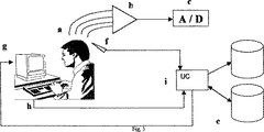
【図3】 この図は、TPECを得るためのシステムを示す図であり、TPECcの特定の実施形態について、汎用性を失うことなく、以下に提示する部分から成る。これらの要素は、次に記載され、その識別のために用いられる文字によって示される。a)被験者の身体に近接して配置される、複数の外部電界および/または磁界センサ。TPECcの場合、前記センサは、患者の頭部に近接して配置される。TPECkの場合、前記センサは、患者の胸部に近接して配置される。これらのセンサは、電子前置増幅器と、前記センサによって取り上げられた信号を記録し、後のアナログ/ディジタル変換のためにこれらの信号の予備調整を行う増幅器から成る、増幅サブシステム(b)に接続されている。増幅サブシステムは、増幅信号を一連の二進数に変換する、アナログ/ディジタル変換サブシステム(1・c)に接続されている。前記アナログ/ディジタル変換サブシステムは、制御ユニット(CU)として動作する汎用ディジタル・コンピュータに接続されている。(i)デジタル化した信号は、CUのメモリに格納され、一方CUは外部ディジタル記憶サブシステム(d)に結合され、以下の読み取りおよび格納を可能にする。
・頭部および胸部それぞれの基準系における脳または心臓の解剖図解。
・他の生物物理的手順によって得られ、頭部または胸部の基準系において定義
された被験者の脳および心臓の機能画像。
本システムは、センサの位置を検出し、ディジタル形態でこれらセンサの座標、および被験者の頭部または胸部の外部解剖学的構造の座標を伝送するデバイス(f)も備えている。これらの座標は前記基準系において定義され、CU内に格納されている。加えて、本システムは、CUに接続され、聴覚視覚的刺激、および患者の神経または心臓血管系を刺激する目的のための熱、電気、および磁気パルスを放出する、複数の刺激デバイス(g)を備えている。また、CUには、研究対象被験者の運動的、生理学的、および言語的反応(被験者の応答)を測定する、複数のセンサ・デバイスが接続されている。CUは、(i)研究の実施を制御するための命令群(プログラム)が常駐するメモリを有する汎用コンピュータである。このプログラムによって制御されるTPECのためのシステムの活動は、(被験者の反応を探求する目的で考えられた)既定の設計に応じた刺激デバイスの活性化、EEG/MEG/EKG/MKGの獲得の制御、センサ位置の決定、EEG/MEG/EKG/MKGと同じ時間基準系における研究対象被験者の活動の記録、その他の生物物理学的様式(modalities)から来る機能画像の獲得、および脳の機能状態の時間的進展の三次元統計的マップを構築するための被験者の研究において獲得した全情報のディジタル処理を含む。
【図4】 Talairach基準系における確率的脳図解の皮膚上に示すEEGの記録のための標準的な10/20システムの電極。
【図5】 任意形状の表面Sに包囲された区分域Rjに対する相互性の原理の図。基本電圧
【図7】 等方性個別均質立体的導体(IPHC)の図式表現)。
【図8】 被験者との処理のシーケンス。TPECを終えるための前述のシステムの使用は、以下の動作から成る。前述のシステムに近接した着座または横臥位置へのお被験者の配置。EEG/MEG/EKG/MKGの記録の形態で、脳および心臓の恣意リ学的活動を表わす電気および磁気信号を検出および記録するためのセンサ群(電極および磁気センサ)の配置。CUのメモリに格納するための、センサの座標および頭部または胸部の外部解剖学的構造の座標の測定のためのデバイスの使用。CUのメモリに格納されているプログラムによって制御された、被験者のデータ収集の開始。増幅およびアナログ/ディジタル変換のためのシステム使用による、被験者の脳または心臓の電気的および/または時期的活動の収集およびアナログ/ディジタル変換。このステップは、任意に、前述のデバイスを用いた刺激の発生、および被験者の応答の獲得を伴うことも可能である。取り込んだ信号は、EEG/MEG/EKG/MKGの時系列の形態で格納する。システムからの被験者の退出。アーチファクトおよび非生理学的周波数成分の除去のため、被験者から記録した信号の予備処理。
プログラムによって用いられる動作のシーケンス。
観察データの入力(任意に、fMRI,PET,SPECTのような機能画像のEEG/EKG;MEG/MKG)。
センサ位置の入力。
解剖図解の入力。これは、個別のまたは確率的構造画像のいずれでもよい。
センサ位置の、解剖図解の基準系への変換。
解剖図解から得た先験確率の算出。
導電特性の入力。
変更したセンサの位置を用いた、電気および磁気LFの算出。
PEC j(t)の算出。
既に予備処理した信号の観察可能な記述パラメータ(DP)の算出。これらのDPは、確率プロセスのモデルの十分な統計である。限定するのではないが、特に、これらの統計のインスタンス(instance)は、次の通りである。
・時間的不変量として、または代わりに非静止として算出した、平均、分散、共分散、または高次累積率。
・時間的不変量として、または代わりに非静止として算出した、記録EEG/EKGおよびMEG/MKGの全チャネルの相互多スペクトル。
・パラメトリック(線形、二次系)および非パラメトリック双方のEEG/EKGおよびMEG/MKGに嵌め込んだ多変量自己回帰関数。
・EEG/EKGおよびMEG/MKG間の相関測定、相互情報、Granger因果律。
・システムまたは被験者の回答によって発せられる刺激に対する前述の種類のあらゆるパラメータの回帰係数。
【図9】周波数ドメインにおけるTPECの正規変動を記述する式を示す。各サブ・プロットは、代表的な脳格子の点に対して、周波数(x軸)および年齢(z軸)に関するPEC(z軸)のスペクトルの対数の回帰表面を示す。
【図10】左前頭頂領域に神経膠星状細胞腫が診断された27才の女の患者から得た、周波数ドメインにおけるTPECcのZ画像。比較の目的のため、この患者の他の画像方式を、b)螺旋CAT、c)SPECT、およびおよびe)T2 MRIで示す。
【図11】a)左およびb)右中)内側脳動脈の脳血管性災害がある2人の患者の、周波数領域におけるTPECcの対数のZ変換の最大強度投影図。
【図12】複合部分的発作を有する患者のEEG記録。この記録は、スパイクおよび波動活動を示す。
【図13】PECの主要源を示し、更に、非線形非静止作用の測定によって決定された情報の流れの方向を示す、図12の記録の時間ドメインにおけるTPECc。[0001]
(Technical field)
The present invention comprises a system and method for obtaining a tomographic image of a primary electric current (PEC) generated by brain neurons and heart muscle cells.
[0002]
(background)
In the present invention, phrases and terms used in the art are defined as follows.
Vectors are shown in bold lowercase letters, and matrices are shown in bold uppercase letters. 1NIs one N dimension
![]()
The primary current (PEC) jp (r, t) is the microscopic magnitude obtained by the spatial and temporal average of the post-synaptic activity of a nerve or heart cell group at location r and time t. It is.
Solid conductor Ωv: The inner area of the body, head or chest under study.
Generated solid Ωg: Ω in which PEC occursvA subset of the brain or heart.
Three-dimensional conductor grid Rv: NvDiscrete group of points rv∈Ωv.
Generated solid lattice Rg: NgDiscrete group of points rg∈Ωg.
![]()
Electroencephalogram (EEG) and electro-cardiogram (EKG): position r on the head and chestc(Recording electrode) and rfIn (reference), voltage difference V generated between a pair of electrodes arranged on the bodyerA time series obtained by measuring (t). Ver(T) is N of the bodyeMeasured at the site. This type of measurement vector is denoted by v (t).
Magnetic brain radiograph (MEG) and magnetic electrocardiogram (MKG): center of simple coil rcVector n of the magnetic field density vector perpendicular to the plane containing itcProjection b abovecnA time series obtained by measuring (t). These simple coils are connected to a superconducting quantum interference device (dc SQUID) by a group of magnetic current detection transducers. The vector of this type of measurement is denoted by b (t).
Anatomical image: A type of medical image that provides structural information about the body such as post-mortem cross-section of the head using computed tomography (CAT), magnetic resonance imaging (MRI), cryotomy.
Anatomical illustration: An anatomical image of the brain or heart in the reference system of the head or chest, respectively. A specific instance of the reference system for the brain is the “Talairach” international system. Possible forms of anatomical illustration include:
Individual structural images of the study object (Figure 1).
Probability: composite statistical image summarizing the intra-individual variability of normal or abnormal morphology of anatomical images in a given population (valdes P. and Biscay R. the statistical analysis of brain images. In: Machine of the Mind, E. Roy Hohn et al. The, (ed.), (1990), Birkhauser, pp. 405-434; standardized tairaiach space.J Computation Assistis. Tomogr 18 (2); 192-205; Evans AC, Collins DL, Mills SR. Evans, A. C., Collins, D. L., Neelin, P., MacDonald, D., Kambei, M., and Marret, TS> (1994) Three-dimensional correlative imaging: ications in human brain mapping.In R.Thatcher, M.Hallet, T.Zeffiro, E.Roy John and M.Huerta (Eds.) Functional neuroimaging technological foundations, Academic Press).
[0004]
Functional imaging: medical information providing information on hemodynamics corporate metabolism, such as functional magnetic resonance (fMRI), positron emission tomography (PET) and single photon emission tomography (SPECT) A type of image.
![]()
Multivariate Z transformation of random variable vector
[Equation 5]
xΘx= {Ux, Σx} Its mean vector, and
![]()
Function space: A set of functions having common characteristics (Triebel, H. 1990. Theory of Function Spaces II, Basel; Birkhauser). A desired property in the TPEC to be considered is specified using membership in the function space. A function space is thought to consist of a combination of atoms.
[0005]
![]()
![]()
Sobolev space with maximum smoothness (for derivative of degree m) (Sobolev)
![]()
![]()
Reference group: consists of a reference group whose membership is to be probable for a given TPEC image.
Classical quantitative electrophysiology (qEEK / qEKG)
As prior art of the present invention, there is research conducted for the purpose of quantifying and detecting abnormal states of the brain and heart by applying multivariate statistical analysis to EEG and EKG. These methods are known as electroencephalography and quantitative electrocardiograms (abbreviated as qEEG and qEKG, respectively). qEEG systems and methods are described in U.S. Pat. Nos. 4,846,190, 4,913,160, 5,282,474, and 5,083,571. Was described in US Pat. No. 4,974,598. These patents explain in detail:
Recording EEG and / or EKG (v (t)) by multiple sensors.
As an option, instead of analyzing the originally recorded v (t), a pre-processed sequence (by calculating the mutual covariance of v (t) for the time series s (t) and the external event marker ( PPS). In the case of EEG, s (t) can be viewed as a series of Dirac delta functions that indicate when certain types of stimuli are applied to the test subject. The resulting time series is known as the average evoked potential (AEP). In the case of EKG, s (t) can report the generation of R wave of EKG itself, and the obtained PPS is an average EKG (AEKG).
[0006]
Extraction of description parameters (DP) from these time series. These are statistical summaries of recorded time series designed to reflect variations in normal and abnormal physiological activity.
In the aforementioned patents, the DPs specified for EEG are averages in the wideband frequency spectrum, including the basic transformations of these DPs. Broadband spectral analysis (BBSA) DP is formally defined as: Let So (ω) be the cross spectrum or variance and covariance matrix of the Fourier coefficients of V (t). DP-BBSA
![]()
In the above-cited patents, the DP for AEP and AEKG is defined as a Karhunen-Loeve base coefficient. These parameters are known as Factor Analysis loading.
The cited patent performs DP conversion and guarantees its gaussianity.
![]()
In the previously cited patent, the population average μxStandard deviation forxComparison of DP is done for normal variability by univariate z-transform expressing DP as deviation measured in units of. Z based on normative databasexIn the calculation of, the effect of concomitant mutations (as in the subject's age) that generate variability that is not the diagnostic object is eliminated by equal variance polynomial regression.
Construction of brain and heart local maps (TM). In these TMs, a subject's deviation from the gnome is encoded by a color scale. TM is an image interpolated between sensor measurements and represents a schematic two-dimensional projection of the head or chest.
Use of cluster analysis to define similar groups of subjects according to their DP values (US Pat. No. 5,083,571).
Using linear discriminant analysis, the test subject is classified as belonging to a diagnostic group, ie, a diagnostic group predefined by cluster analysis based on a default value of the DP (US Pat. No. 5,083,571). issue).
[0007]
A statistical distance measure for the subject's previous state performed at the selected time point. This provides information about the physical state of the subject. For example, the state is as follows. During surgery, intensive care, or evaluation for pathology evaluation (US Pat. Nos. 4,545,388, 4,815,474, 4,844,086 and 4,841,983) . The utility of these methods has been confirmed in several studies (John, ER; Harmony, T. Valdes-Sosa and P. (1987b); The uses of statics in electrophysiology. In: Gevins, A. S. and Remond, A. (Eds), Handbook of Electroencephalography and Clinical Neurophysiology. Revised Series. Volume 1, Elsevier, The. , P. (1987a); Normative data base. and neurometrics. Basic concepts, methods and results of norm construction.In:Gevins,A.S.and Remond, A. (Eds), Handbook of Electroencephalography and Clinical Neurophisiology.Revised Series, Volume 1, Elsevier, The Netherlands, 449- 496). However, these methods have the following limitations.
[0008]
DP-BBSA is insufficient as a descriptive parameter for quantifying the many types of EEG activities. This is due to loss of resolution due to frequency band averaging, resulting in a loss of sensitivity and specificity in diagnosis (Szava, S .; Valdes, P .; Biscay, R; Galan L .; Bosch, J .; Clark, I. and Jimenez, JC: High Resolution Quantitative EEG Analysis. Brain Topology, Vol. 6, Nr. 3, 1994, pp. 211-219).
Analysis of the DP group by using TM is hampered by the high correlation between variables. To overcome this difficulty, Galan et al. (Galan, L; Biscay, R; Valdes, P .; Neira, L. and Viruses T. (1994); Multivariate Strategic Brain Electromagnetic Mapping, Brain Topology, Vol. Introduced multivariate TM.
The assessment of TM normality is made by univariate statistics without taking into account the need for control of type I errors caused by multiple comparisons to multiple points in the map. This increases the probability of erroneous abnormality detection to an uncontrollable level.
![]()
The use of magnetic measurements b (t) is not included despite the fact that they add additional information to the information provided by V (t).
The analysis of physiological information has no reasoning about j (t) and is limited to v (t). Therefore, none of these methods calibrate the TPEC format. They merely analyze the projection of j (t) on the surface of the body after being distorted by the subject's tissue interposed between the generator / sensor of the nerve / heart PEC. In fact, the relationship between PEC and EEG / MEG / EKG / MKG depends on the conductor properties of the head and chest (eg, geometry, conductivity, electrical and magnetic permeability, etc.)
Brain and heart multivariate statistical map
Some of these constraints are described in Pedro Valdes-Sosa et al. U.S. Pat. No. 5,282,474. This patent claims to use statistical methods for the assessment of abnormal brain and heart activity with the following innovations:
Add b (t) as an optional physiological information source. Subsequently, the use of DP obtained from both v (t) and b (t) is included in the definition of qEEG and qEKG.
A marker of the more general form of external events, or those derived from their own analysis o (t), where the additional components of the time series s (t) are obtained from the subject's own spontaneous or involuntary response It is included in the form of A sequence derived by such call processing is named an event-related component (ERC) derived from o (t).
[0009]
ERC extension in functional space-time tensor product. These include not only the fundamentals of Fourier, but also wavelets between different DP sets (for the description of non-statistical processes) that increase flexibility in the description of physiological processes.
These DPs are summarized by using higher order statistical moments and different parametric time series models. In particular, linear autoregressive coefficients are included.
Introduction of DP as a high-resolution interval analysis (HRSA) consistent in the use of So (ω) for all frequencies ω by a variant of discrete Fourier.
Introduction of color scale in TM based on empirical probability distribution of global maximum and minimum of DP. This scale provides effective control of the probability of false anomaly detection.
The improvement to brain activity assessment introduced in this patent is illustrated.
By construction of HRSA gnomes for Cubans aged 5 to 97 (Valdes, P .; Biscay, R .; Galan, L .; Bosch, L .; Szava, S .; and Viruses, T .: High Resolution Spectral EEG norms for topography, Brain Topology, 1990, vol.3, pp.281-283 and Valdes, P.; Bosch, J.; Serius of it Banks, R .; and Biscay, R ,: Frequency domain models for the EEG.Brain Topography, 1992a, vol.4, pp.309- 319).
By demonstrating that DP-HRSA achieves higher sensitivity and specificity than DP-BBSA for detection of neurology and psychological pathology (Szava, S .; Valdes, P .; Biscay, Bosch, J .; Clark, I. and Jimenez, JC: High Resolution Quantitative EEG Analysis, Brain Topology, Vol. 6, Nr. 3, 1994, pp. 2111-219). .
However, the construction of the o (t) DP used in this previously cited patent is limited to a parametric model such as DP-HRSA. There is a complete description only for o (t) for stationary and linear stochastic signals, or signals with a limited kind of nonlinearity. The ineligibility (especially patients with aneurysm) of EEG studies of certain subjects with such DP was illustrated by Hernandez, Valdes-Sosa and Vila (Hernandez, JL, Valdes, PA). , And Vila, P. (1996) EEG spike and wave modeled by to stochastic limit cycle, NeuroReport, 7: 2246-2250).
The qEEG method and qEKG do not apply to the estimate of j (t) because they are not true variants of TPEC.
[0010]
Tomography of brain and heart primary currents
As in all types of tomography, the starting point for the development of TPEC is the probability of a model relating observation data to an estimated amount, which is known as a direct problem. In TPEC, the direct problem is how to generate o (t) from j (t). This model has two components.
Specific models of assumed conductive properties, i.e. head and chest conductive properties, in particular their geometry, conductivity, electrical and magnetic permeability etc.
Model assumed for j (t), or source model.
The characteristics of the three-dimensional conductor areE(R) and magnetic kM(R) Summarized in the lead field (LF). These are PEC jp(R, t), ver(T) and ben(T) is a kernel of the first kind of Fredholm-type integral equation that probates a direct relationship.
[Expression 18]
![]()
![]()
Instead of the classical Green formulation, the problem is formulated directly using LF, and Rush and Driscoll (Rush S. and Driscoll DA AEEEG electrodesitivity-an application of reciprocityEcE , Eng., Vol. BME-16, pp. 15-22, 1969) and Plonsey (Plonsey R. Capability and limitations of electrocardiography and magnetocardiography, IEEE Trans., Bio. pp. 239-244, 1972 ) Gave me a remarkable advantage. This is mainly because all of the head and chest conductive properties can be abstracted at these sizes without assuming a specific model for PEC. However, it is well known that the conductivity in the body is inhomogeneous and anisotropic (Hoeltzell P.B. and Dykes RW Conductivity in the somatosensory of the cat.Evidence for corticotropy. Research, 117, pp. 61-82, 1979), in practice, the calculation of LF is very complicated. However, for each tissue type that calibrates the area, significant simplification is possible if the conductivity is considered constant and isotropic (Schwan HP and Kay CF, the conductance of living tissues). , Ann, NY Acad, Sci., Vol.65, pp.1007-1013, 1957). This model of the three-dimensional conductor is named as an isotropic individual homogeneous three-dimensional conductor (IPHC: Isotropic and Piecewise Homogeneous Volume Conductor). In general, two types of model IPHC are used for the head and chest.
Sphere: The simplest model that specifies a surface that defines different areas as concentric spheres. In this model, there is an explicit expression that evaluates K. This model is easy to evaluate, but is not very accurate mainly for the time domain of the head.
Reality: The surface of the area is obtained from an anatomical illustration. For this model, Fletcher et al. (Fletcher D.j., Amir A., Jewett D.L. and Fein G. Improve method for the calculus of potential in E. modal. E. mod. E. modal. E. med. pp. 1094-1104, 1995) and Oostendorp and Osteroom (Oostendorp T. and van Osterom A. The potentially distributed nature of the biomolecules in the homeosphere. y shape.IEEE Trans.Biomed.Eng., vol.BME-38, pp.409-417, 1991). However, this procedure is based on the boundary element method (BEM) for the calculation of the potential difference on the surface that limits the area created by energizing the sensor.
formula
[Equation 19]
[Expression 20]
l (o (t) | j (t), ΣEE) = C0exp [-Rθ] Is defined as the likelihood corresponding to equation (3), and C0Is a constant for density normalization. In the following, it is assumed that po = 2 unless otherwise stated.
[0012]
The central purpose of TPEC is to estimate j (t) by minimizing (4), which is an “inverse problem”. In general, it is well known that (4) has no unique solution. This is because the LF operator has a non-trivial null space even when simultaneous electrical and magnetic measurements are possible.
PEC estimation is possible only if it contributes a priori information in the form of a model for j (t) that enforces a set of constraints. These can be classified as follows.
Exogenous: consists of requiring compatibility of the desired solution with information provided from other types of neural images. Typical requirements for anatomical neuroimaging of the brain are
Estimating j (t) only inside the spherical solid conductor that models the head;
j (t) is limited to the subject's cortical plane and oriented perpendicular to the cortex (Dale, AM, and Sereno and MI, J. Cognit. Neurosc., 1993). 5: 2, pp. 162-176).
Endogenous: consists of requirements regarding the shape and area range of the activated tissue. It is necessary to keep the activation area as small as possible while maintaining the compatibility between the model and the data (simpleness). For shape variations in space j (t), this requirement ranges from a minimum smoothness (a collection of Dirac deltas corresponding to the current dipole) to a maximally smooth function.
All of the above conditions are forced into the solution in two equivalent ways.
Regulation: (4), non-negative function RJ= RJAdd (j (t) | Θ) and minimize.
![]()
Bayesian estimation: maximizing a posteriori distribution
[Expression 21]
![]()
The fundamental difference in the different methods developed to estimate the generator of o (t) is in the model specified for j (t). These will be reviewed as follows.
RJ(J (t) | Θ) is Ng<Θ0If the function guarantees0If is a constant, the uniqueness of the solution of equation (4) is guaranteed. This class of models for j (t) is termed the current dipole (Scherg, M. and Ebersol, JS (1993); Models of Brain Sources, Brain Topology, Vol. 5). Nr. 4, pp. 419-423).
[Expression 22]
These are effective for modeling the situation where a small group of regions generates a PEC and all are small ranges.
Formalization provides a simple least squares estimation method.
The set of estimated DPs obtained is very compact and consists of the position and orientation of each current dipole.
Due to the simplicity of the model, it is easy to place additional constraints on the estimation of this model of PEC (Scherg, M. and Ebersol, JS (1993); Models of Brain Sources. Brain Topography, Vol. 5, Nr.4, pp.419-423). For example, αgA certain degree of smoothness can be imposed on (t), and μg(T) = μgThe requirement is not time dependent. These requirements stabilize the estimated DP.
[0014]
However, the dipole model discussed has the following constraints.
PEC (NgIf the number of possible generators) is too large, this type of model frequently requires manual operator intervention. In this case, the inverse problem is also solved by mistake. In fact, these models are NgDoes not include statistical methods to determine
If different regions of the tissue generating PEG are spread over a wide area, the dipole model estimates an equivalent dipole located at the center of mass of the actual region, thus creating artifacts.
αgThe smoothness of (t) is enforced by the use of spline basis, and the possible form of activity spread is represented by the Sobolev function space W2(L2) (Two-time derivative integral Lebesgue).
This type of model has only been used to describe AEP or AEKG.
This generator model is applied using a three-dimensional conductor sphere or a real model. However, the LF methodology is not used, and in practical cases it is necessary to use a numerical algorithm. These are not very practical because they require evaluation of the BEM process for each iteration.
TPEC is described in Valdes-Sosa et al. U.S. Pat. No. 5,307,807, first proposed and gave status to a new style of medical imaging. The present invention consists of a method and system for creating a three-dimensional map of the width, orientation and conductivity of a neuro / cardiac PEC generator with the following innovations.
Perform an estimate of j (t) on the inner three-dimensional lattice in the body.
Consider the CRE PEC DP.
Information obtained from other types of structural medical images is used to identify the conductive properties of the subject's body. This is also used to determine the spatial range of the grid that predefines the PEC (thus limiting the possible sites for estimating the PEC) and determining the orientation of the PEC. The subject's body geometric properties are quantitatively incorporated into the PTEC through the use of a parametric model.
[0015]
Information about substance metabolism of the subject under study obtained from other types of functional medical images is used to further limit the grid for estimating j (t).
The modeled generator not only contains individual sources (dipoles) but also spreads the generator describing the background generator noise if it is wider than the individual generators.
Introducing frequency domain estimation into the generator of the CRE, in particular the generator cross-spectral matrix Sj(Ω) is introduced. The improvements to the assessment of brain activity introduced in this patent were later verified by studies on the original abnormal electrical activity in subjects with localized nerve lesions. For example, Harmony, T .; Fernandez-Bouzas, A .; Marosi, E .; Fernandez, T .; Valdes, P .; Bosch, J .; Riera, J .; Rodrigues, M .; Reyes, A .; Silva, J; Alonso, M .; and Sanchez, J .; M.M. (1995): Frequency Source Analysis in Patents with Brain Relations, Brain Topology, vol. See 2.
However, the aforementioned clinical studies and others (Valdes, P .; Carvallo, JA; Alvarez, A .; Diaz, GF; Biscay, R .; Perez, MC; Szava, S .; U.S. Pat. Nos. 5,282,474 and Virues, T. and Quesada, ME: qEEG in to public Health System, Brain Topology, Vol.4, Nr.4, 1992b, pp. 259-266). The invention described in US Pat. No. 5,307,807 did not consider the following aspects necessary for further completeness of the TPEC methodology.
The statistical procedure described in US Pat. No. 5,282,474 has not been extended for use in TPEC. In other words, the sample space of TPEC is a random field defined on a four-dimensional spatio-temporal manifold, so a special method is necessary for this analysis, but it is not considered in the patent. It was.
The regression method used in US Pat. No. 5,282,474 to eliminate the effects of experimental adjoint variables is of the parametric global polynomial type. They are not flexible enough to describe the variations in multiple scales typical of electrophysiological data.
In the case of US Pat. No. 5,307,807, only the regulated source consists of controlling the number of dipoles that consider the parameters. This is Ng<Θ0Function R that guaranteesJIt is an implicit use of (j (t) | Θ), is not very flexible and requires frequent human intervention.
In U.S. Pat. No. 5,307,807, a solution to the direct problem relating generator activity to an observable signal is obtained by anatomical deconvolution. This method does not fit the general configuration of the generator and is only an inaccurate numerical approximation to the optimal solution.
[0016]
In the case of US Pat. No. 5,307,807, the parametric description employed to characterize the subject's body geometry is based on the use of a quantitative description of the functional form, and morphological variation within the solid. There is not enough flexibility to describe the sex appropriately. That is, this method cannot include probabilistic anatomical information if it is not desirable or practical to obtain a structural image of a particular subject under study.
In the case of US Pat. No. 5,307,807, the substance metabolism information obtained from other image formats is only integrated as a constraint on the region where active dipoles are allowed. This information is therefore not used for statistically optimal estimation procedures.
Since the publication of the aforementioned two patents, a series of studies have emerged, which have not fully solved the problem outlined above, but have contributed to the refinement of the solution claimed in the present invention. The relevant developments are then listed together with an assessment of their advantages and inadequacies.
The DP that has been used in the construction of all TPECs to date is either raw data or sufficient statistics derived from that data, almost always one of the lower order statistical moments in the time or frequency domain. Part. A recent study (Hernandez, JL, Valdes, PA, and Vila, P. (1996) EEG spike and wave modeled by stochastic limit cycle, NeuroReport, 7: 2246-2250). We demonstrate the need for a flexible non-parametric description for the temporal sequence of EEG / MEG / EKG / MKG that allows the description of dynamic activity, particularly nonlinearity, which is characteristic of tissue mass.
![]()
(Riera, J.J., Aubert, E., Valdes, P., Casanova, R. and Lins, O. Discrete Splay Electric Electric-Magnetic Tonemography (DSPET) based on Realistic Energy. BIOMAG'96, Santa Fe, New Mexico, February 1996). Here, the smoothness of the solution is the matrix ΣJJSpecified by. The PEC estimator in this case has the following explicit representation:
[Expression 24]
![]()
The most important representative in this TPEC line is ΣEE= Σ2 EEIs characterized by assuming |. Where σ2 EEIs a common distribution for the same type of sensors. By assuming different linear solutions as shown below, ΣjIs characterized by
![]()
[0018]
Low resolution electrical tomography (LORETA).
[Expression 28]
![]()
![]()
[Expression 29]
In some cases, additional constraints can be added to obtain the well-known Backus and Gilbert solution described in US Pat. No. 4,977,896.
All of these spline methods are related to the Sovorov space Hq(L2) Specifies the membership of j (t). This is too restrictive since estimation of dipole PEC is not allowed. In fact, Rayleigh bounds are valid and describe the impossibility of discriminating nearby point sources. In addition, this limit is responsible for the appearance of “ghost” solutions and interferes with artifacts due to the limit of solutions by linear methods.
[0019]
Several authors have proposed a non-linear estimator for j (t) in search of a solution with less spread. Among them, 1) Matsuura and Okabe (Matsuura L. and Okabe Y. (1995) Selective Minimum-Norm Solution of the Biomagnetic Inverse Probe. IE tran. In the generalized Gaussian distributionoAnd pjAs a result, the inverse solution must be estimated nonlinearly. 2) Gorodnitsky and Bhaskar (Gorodnitsky, I.and Bhaskar D.R.1997 Sparse signal reconstruction from limited data using FOCUSS:.. A reweighted minimum norm algorithm IEEE Trans.Signal Proc.Vol.45 (3) pp600-616) is It has been proposed to apply the estimator of equation (5) repeatedly and weight each grid point in proportion to the j (t) value estimated in the previous step. Both proposals algorithmically converge to a number of individual generators equal to the number of sensors, and thus actually become a more elaborate form of dipole fit. As a result, they share the flaw of not being able to estimate spatially distributed point sources with these dipole models.
Philips et al. (Philips JW, leahy RM and Mosher JC. MEG based imaging of focal current sources sources. (1997). IEEE trans Medical Imaging, Volume 3: 38). did.
[30]
![]()
![]()
[31]
![]()
Numerous studies have achieved processing of o (t) images, sometimes taking into account information contributed by other neuroimaging formats, but for the purpose of estimation and subsequent use of j (t) It should be stated that there is no. This is the case with Finnish patent 925,461 and US Pat. No. 5,331,970. Since these patents are not aimed at obtaining TPEC, the analysis of this technology does not include these types of prior art.
[0020]
(Description of the invention)
An object of the present invention is to provide a system and method for calculating an estimate of j (t) based on o (t), where the estimate is denoted as TPEC. Referring to brain research, specifically, in the brain primary current tomography, the procedure is shown as (TPECc), and in the case of the heart, it is shown as heart primary current tomography (TPECk).
The map specifies a) a constraint for a structure with a high probability of generating electrical activity using an anatomical diagram due to this constraint, and b) a pre-specified where the solution is defined by a Besov-type, or mega dictionary It is an inverse solution to the EEG / MEG / EKG / MKG problem based on forcing it to belong to a function space. The probability that this map or a subset thereof belongs to the examination group is determined. Because of this limitation, we model the spatial and temporal correlation of the map, as well as the dependence on experimental covariables. The resulting probabilities are encoded on a pseudo color scale and overlaid on the anatomical illustration for their interactive 3D visualization. The illustration used for solving and visualizing the inverse problem can be an individual structural neuroimage, a stochastic illustration, or a plastic deformation from a stochastic illustration to an individual morphology.
[0021]
Accordingly, one aspect of the present invention comprises a primary current tomography (TPEC) system of the brain (TPECc) and heart (TPECk),
A primary current tomography (TPEC) system of the brain (TPECc) and heart (TPECk) comprising the following elements:
A plurality of external electric and / or magnetic field sensors placed close to the subject's body and connected to the amplification subsystem, placed close to the subject's skull for TPECc and close to the subject's chest for TPECk Arranged with a sensor,
An amplification subsystem consisting of a preamplifier and an electronic amplifier, which records the signal detected by the sensor and preconditions the signal for its analog / digital conversion;
An analog / digital conversion subsystem that converts an amplified signal into a sequence of binary numbers o (t) and stores the sequence in a memory of a general-purpose digital computer that functions as a control unit (CU). In the case of TPECk, the time series obtained from the electric sensor is an electrocardiogram (EEG), and the time series obtained from the electric sensor is an electrocardiogram (EKG). An analog / digital conversion subsystem that is a diagram (MKG);
-Input to the reference system of the head and chest of the anatomical illustration of the brain or heart, coupled to the CU, and the conductivity, electrical and magnetic permeability inputs associated with the tissue described in the illustration An external digital storage subsystem that enables a specific and non-exclusive instance of the reference system of the brain to be the “Tairaach” international system;
An external digital storage subsystem coupled to the CU, where the CU has other functionalities such as Functional Magnetic Resonance Imaging (fMRI), Positron Emission Tomography (PET) and Single Photon Emission Tomography Photons (SPECT) An external digital storage subsystem that allows input of an image of the functional state of the subject's brain or heart obtained by a biophysical procedure, wherein the functional image is defined in a head or chest reference system;
A sensor position detection device, in digital form, which communicates the coordinates of the sensor and the external anatomy of the subject's head or chest, wherein the coordinates are defined in a reference system of the head or chest and the CU A sensor position detection device stored in
A plurality of stimulation devices connected to the CU and emitting auditory visual stimulation and heat, electrical and magnetic pulses for the purpose of stimulating the patient's nerves or cardiovascular system;
A plurality of sensor devices that measure the motor, physiological and verbal responses (subject responses) of the subject under study;
A CU having a memory in which a group of instructions (programs) for controlling the implementation of research is resident, the program operation area being an activation of a stimulation device according to a predetermined design, EEG / MEG / EKG / MKG Construct a three-dimensional statistical map of control of acquisition, sensor location determination, recording of subject activity, acquisition of functional images from other biophysical modalities, and temporal evolution of the functional state of the brain Including digital processing of all information acquired in the subject's research for
Consists of.
[0022]
In addition, the present invention also provides a calculation method for use with the above-described system, which comprises the following steps.
a) Conversion of anatomical illustration of sensor coordinates (FIG. 4) to a reference system. This is accomplished by providing viscoelastic deformations (most commonly non-linear) and maps the coordinates of the subject's external anatomical markers to the anatomical illustration stored in the CU.
b) Calculation of linear operators (electrical and magnetic kernels) that predict EEG / MEG / EKG / MKG generated in subjects with PEC in either part of the brain or heart. This kernel is calculated for the lattice using the principle of electrical and magnetic reciprocity. This principle establishes a linear relationship between electrical and magnetic LF, and when the sensor is energized with low frequency direct current or alternating current, an electric field appears. This electric field therefore summarizes all the conductive properties of the heart or chest, regardless of the appearance of any CEP. Reciprocity theorem. δr3The conductor ΩvIt is an internal three-dimensional element. Position r inside the conductorgPrimary current jp(T) δr3The point source is the electrode lead located on the skull.
[Expression 33]
[Expression 34]
![]()
[0023]
From the above procedure, a large system of algebraic equations is obtained. The use of multi-solution analysis based on the principle of thresholding enables the conversion of these enormous algebraic systems into sparse formats, thus greatly reducing the cost of computation and errors caused by rounding. (D. M. Bond and S. A. Vavasis. Fast wavelet transforms for matrixes forming foundation element methods, 1994 and Growinski R., W. T. O. Wavelet and finite element solutions for Neumann problem using fititious dome ins, 1994).
c) Determining possible locations of PEC generators in the head or chest by using anatomical illustrations
In the special case of isotropic individual homogeneous solid conductors, the aforementioned IPHC is divided into N sections (R1, R2, ..., RNThese are arranged so that they do not intersect and do not include the sections. Air is RN + 1It is defined as In addition, σjIs the RjRepresents the value of conductivity at (σN + 1= 0). Surface Sj, j + 1Is the RjAnd Rj + 1Is the boundary that separates Vector nj(R) shows a normal line r to the surface of the position (FIG. 7).
1) Each zone R for situation (1)jOhm current density atj(R) corresponds to the vector boundary problem and can be calculated based on the second green vector equation.
[Expression 35]
[Expression 36]
[Expression 37]
Equations (11) and (13) are solved analytically if the IPHC symmetry allows expression in a curvilinear coordinate system that allows separation of variables for the solution of the Laplace vector equation. Otherwise, they must be converted to Cartesian coordinates and discretized. In (13), the fixed frequency ω = ωcFor these equations, the independent term {j∞(R), j∞(R, ωcNote that there is only a difference in)}. General vector field ck(R) = {jk(R), jk(R, ωc)}. Then this is the independent term c∞(R) can be written, and this general vector field satisfies:
[Formula 38]
![]()
[39]
![]()
The solution of the system of algebraic expression (17) is the system cest= (D + Γ)-1C∞Is obtained by reversing the matrix of This algebraic system has no singularity problem. This is because the ohmic current density does not depend on specifying any criterion.
Division RjC at point r insidejThe value of (r) is obtained by substituting the general vector field estimated on the surface into the following equation.
[Expression 41]
About EEG
With the in mind that the injected current is considered constant for all triangles marked on the skull, both corresponding to the electrical, we obtain:
[Expression 42]
Fixed frequency ω = ωcIf the magnetic field vector density is constant in each triangle and is equal to the value at the center of mass, the following equation is obtained.
[Equation 43]
(44)
Calculation of reverse solution
The solution to the inverse problem is based on the formulation of a hierarchical Bayesian model for image fusion (Hurm, 1996; Mardia, 1996). At the most basic level of the model, we assume the presence of unobservable brain or heart tissue activity A (t).
This model consists of the following components:
• Likelihood term I for each style m based on the corresponding direct problemom
[Equation 45]
![]()
![]()
Each function activity F adjusted for brain activity A (x, t) according to the following relationshipmA priori probability π for each (x, t)fm
[Equation 47]
![]()
![]()
Brain or heart activity A (t) to πA(A (t) | ΘA) A priori probability πA
・ A priori probability for hyperparameters
ΘA ~πΘA(ΘA)
Θβm ~πΘβm(Θβm)
Θem ~πΘem(Θem)
All of these lead to a priori probabilities on the following basis:
[Formula 48]
Model parameters A, ΘA, F, Θβ, ΘEAll estimations are made by the maximum method a posteriori (MAP) method. Some embodiments of the present invention have explicit estimators. Otherwise, the estimated value is obtained by one of the following iterative methods, and the initial value is a simpler model or simply an estimated value of a random value.
Parameter A, ΘA, F, Θβ, ΘEIterative Conditional Maximization (ICM: Winker, G. (1995) Image Analysis, Random Fields and Dynamic Carries) Methods Mounts. Springer).
A. “Expectation Maximization” (EM: Tanner, 1996) which continuously maximizes (20) for a subset of parameters and fixes other parameters to their expected values.
B. Mode selection of the Monte Carlo distribution of (20) obtained by Monte Carlo Markov Chain methods (MCMC, Tanner M. 1996 Tools for Statistical Inference. Third Edition, Springer).
The advantage of formulation (20) is that it allows a combination of different temporal and spatial resolutions of the information provided by the imaging modality in a statistically optimal manner. The weight to be assigned to each style is automatically obtained. That is, it is possible to find the optimal relative weight to which EEG and MEG should be combined.
The likelihood format is specified in the form of risk.
[Formula 49]
[Equation 50]
[0028]
[Formula 51]
[Formula 52]
In order to find the MAP estimator of (20) using ICM, EM, or MCMC, the essential steps are R0+ Λ ・ RJIt is a minimization of an expression of the form (j (t) | Θ) (Expression 5). R0
[Expression 55]
![]()
![]()
Partial decomposition (Smola, 1996) is equivalent to regression with a support vector mechanism (SVM). In addition to enabling efficient minimization as described for the quadratic programming problem, the resulting solution is robust against data contaminated by outliers. In addition, the estimated PEC is KmIs a function of the reduction in the number of elements and guarantees simplification of TPEC.
EEG and MEG fmFor both (t) = j (t), the PEC model is further refined as follows.
![]()
Specified as Equation (25) extends the spatiotemporal modeling initially introduced into the brain dipole (Equation 7; Scherg, 1993) to TPEC.
j (t) = M · G (t) + ξ (t)
The generator orientation and strength are specified by defining the following a priori probabilities:
[Formula 59]
For the fitness, the brain activity A and the function smoothness predefined by Besov space are enforced. In this case, when the Besov space of the index (1, 1, s) is selected, a variable resolution TPEC (VARITA: Variable Resolution TPEC) is obtained. VARETA allows estimation of both point source and distributed source generators within the same framework. Therefore, the absolute dichotomy between both types of modeling that existed before is no longer necessary. In VARETA, the amount of smoothness applied to the solution can be variable point by point within the generated solid. This was named “variable resolution”. This variable resolution allows for a spatially adaptive nonlinear estimate of the current point source and eliminates the “ghost” solution that exists in ordinary linear distribution solutions. This also makes it possible to achieve “super-resolution” that can distinguish discrete sources that are very close to each other. In particular, although not an exclusive realization, the a priori probability of equation (26) is:
[Equation 61]
[62]
![]()
A similar equation for equation (27) is also apparent. pgNote that due to our dependence on, our a priori knowledge allows a stochastic constraint of the estimator on the PEC for the points of the grid. That is, pgThe constraint on the identification of this PEC becomes deterministic if を 取 る takes only the
[0031]
Statistical evaluation
Determining membership for a test group
Once an estimate of j (x, t) and γ (x, t) and a hyperparameter estimate are obtained for a given subject, these choices are configured in the DP vector. This vector is used in one of a number of test groups to determine whether the obtained TPEC can be classified using non-parametric statistical methods (Ripley BD (1966) Pattern Recognition and (Neural Networks. Cambridge University Press). The test groups representing different embodiments of the present invention are as follows.
A group of subjects defined as normal by an evaluation standard other than TPEC. These groups are implicitly designated by a sample of normal subject TPEC DPs stored in the database. In this case, the purpose of statistical analysis is to determine the probability that an estimated TPEC DP is obtained from a healthy subject.
A group of subjects defined as having a pathology predefined by criteria other than TPEC is implicitly specified by a sample of TPEC DP for patients with the target lesion stored in the database The In this case, the purpose of statistical analysis is to determine the probability of obtaining a TPEC from a subject with a specified disease.
-Groups determined by the method of Unsupervised Pattern Recognition. The TPEC DP criteria for samples of normal and / or diseased subjects commonly have the physiological characteristics of the subject. In this case, the purpose of statistical analysis is to determine the probability of obtaining a TPEC from a subject with physiological characteristics.
A group of TPEC DP samples previously obtained from study subjects. For each analysis time, the DP group constitutes a vector time series. There are two purposes of statistical analysis of this vector time series.
1. It is also an object to determine changes over time in the function of a given part of the brain or heart that are reflected in changes in DP, for example to monitor the state of the brain during surgery.
2. Predict the probability that a DP vector reflecting the functional state of the brain or heart will obtain a given set of values at some point after the current test.
[0032]
For the calculation of previous probabilities, for each of the parameters at each point of the lattice of the generated solid, the mean μxIt is necessary to have (v) and variance x (v). These means and variances can be expressed as a function of the control variable v by non-parametric regression (Hastie, TJ and Tibshirani, RJ (1990): Generalized additive models. Chapman and Hall, Pp18- 20; ISBN 0-412-34390-8 and Fan J. and Gibbels. I. Local Polynomial Modeling and its Applications, 1996).
![]()
1. Transformation to the target distribution with a non-linear function x = T (DP) to confirm that the vector x has a distribution close to one previously specified selection f.
2. Z using a single variation mutantxConversion calculation.
3. zxCalculation of the probability that all or part of will reach a pre-specified maximum or minimum value. This calculation is performed by correcting for the effects of numerous spatial and temporal correlations. These are the results of the estimation process as well as the results of brain and heart lesions, and the overall effect increases Type 1 errors in identifying lesion states.
The complexity of this problem is z as a random function defined on a four-dimensional manifold.xIs in the nature of The three dimensions are space and one is time (as defined without loss of generality, but the time dimension may also mean an extension based on a mega dictionary, so the frequency or time-frequency dimension is May be defined). Statistical methods have been developed for this type of random variable, defined as a stochastic process on an n-dimensional variety (Worsley, KJ, Marrett, S., Neelin, P., Vandal, A. C., Friston, K. J., and Evans, A. C. (1995): A unified statistical for determinating signaling signals in H. cerv. These statistical procedures have been applied to the study of structural images (CAT, MRI) as well as functional images (fMRI, SPECT, and PET). The method described above has not yet been applied to the field of qEEG / qEKG and TPEC. That is, these results are Zmax, Calculate the probability that the maximum value of z observed in the target area C (of any shape) exceeds a given threshold U.
[Equation 63]
Where ρmax(F)dAnd ρmin(F)dDepends on the assumed random field form f (Gauss, t, F, χ2Etc.), RdCharacterize the geometric shape of C expressed in terms of the FWHM of the random field.
[Expression 64]
![]()
![]()
zxIs plotted in the following way.
・ Z as a one-dimensional graphxPlots as a function of the lattice child fixed points. This type of graph is called a TPEC z-image. The plot is performed according to a color code indicating the degree of deviation from the reference value of TPEC. This plot is superimposed on the anatomical illustration that makes up the background of the image.
ZTo clarify the statistical evaluation of images, we define the following transformations:
[Equation 66]
[0034]
Examples of preferred embodiments
TPEC in the frequency domain
One preferred but non-exclusive embodiment of the present invention is TPEC in the frequency domain for EEG. This embodiment is advanced for situations where it is not convenient to obtain individual MRIs, thus requiring the use of probabilistic brain illustrations. Here, observation is performed as EEG for individual i and segment j,
[Equation 67]
![]()
In other words, the observed EEG is the ideal recording EEGv.i, j(T) is multiplied by a scalar coefficient κj (individual and random), and the reference electrode ρijAssume that the distortion is due to subtracting the activity of (t).
Visual inspection ensures that the segments meet the assumptions of stationarity and “mixing” (Brillinger, DR, (1975): Time series.
![]()
[Equation 68]
[Equation 69]
[0035]
Here, H indicates a centering matrix for converting data into an average standard (Mardia KV, Kent JT and Bibby JM. (1979): Multivariate Analysis. Academic Press Inc. London, κ). The likelihood estimator is described in Hernandez et al. (Hernandez, J. L .; Valdes, P .; Biscay, R .; Viruses, T .; Szava, S .; Bosch, J .; Riquenes, A. and Clark, I. (1995) : A Global Scale Factor in Brain Topology. International. Journal of Neuroscience, 76: 267-278).
In this case, the main target purpose is Σji(Ω) is estimated by selecting an appropriate a priori probability. In this case, the MAP estimation procedure is equivalent to minimizing the following equation:
[Equation 70]
[Equation 71]
[Equation 73]
![]()
[0036]
Where the diagonal matrix ΛsSpecifies the smoothness applied to each point of the grid, which in this case is zero for gray matter boundaries. ΛmLoads the allowable size of the PEC at each point of the grid.
![]()
![]()
![]()
![]()
[0037]
SjA two-dimensional or three-dimensional plot of z values obtained from (ω) constitutes an example of a TPEC z-image. The plot was performed using a color code indicating a deviation from the calculated standard value of the image. This plot is overlaid on the brain illustration of the Talairach coordinates that make up the background of the image.ZFor statistical evaluation of the images, assume that these are samples of four 3D Gaussian random fields (3 space and 1 frequency dimension). In this case, Worsley et al. (Worsley, KJ, Marrett, S., Neelin, P., Vandal, A.C., Friston, KJ, and Evans, A.C. (1995): A unified statistical application for determining signing signals in images of cerebral activation. Human Brain Mapping, 4: 58-73). This allows an evaluation of the probability that the maximum or minimum of the image z takes a given value. Z mentioned abovewA transform is chosen to obtain a scale of probability corresponding to a univariate Gaussian distribution.
[0038]
Clinical example 1
In FIG. 10a), a Z image of TPECc in the frequency domain is shown. This image was obtained from a 27-year-old female patient, and astrocytoma was diagnosed in the left frontal parietal region. For comparison purposes, this figure also shows b) helical CAT, c) SPECT, and e) T2MRI.
Clinical example 2
Based on the diagnosis of an ischemic origin cerebrovascular disaster due to occlusion of the left (LCMA) or right (RCMA) medial cerebral artery, a group of 11 recently admitted neurological patients was selected. The TCEPc frequency domain and CAT were applied to all patients. An example of the obtained TPECc-FD is shown in FIG. There is complete correspondence with clinical diagnosis. In case 7, it can be seen that TPECc-DF is superior to CAT, with respect to specific accuracy, three are equal and only one is bad. To date, CAT is an image selection method for evaluation of CVA despite its invasiveness.
[Table 1]
Non-linear analysis of γ (x, t)
Another preferred but non-limiting embodiment of the invention is TPECc in the time domain. In this case, the above-described method is used to identify an active brain region and its functional connections when each subject subject has an individual anatomical brain diagram. Once γ (x, t) is estimated, these are analyzed as non-linear time series. The value of γ (x, t) is a vector that fits a nonparametric nonlinear autoregressive model (NNAM)
![]()
![]()
![]()
![]()
![]()
[0040]
In addition, the estimate of F allows the calculation of the Granger causality estimate between the generators of PEC, due to the subcutaneous non-linear and non-stationary generalization of the influence measurement introduced by Geweke (1984). A, B, C is γtA time series subset of
![]()
[Formula 78]
[Brief description of the drawings]
FIG. 1 Anatomical illustration of the brain based on individual structural images. a) An axial slice of MRI, to which the contour detection procedure was applied. b) Summary of detected skin. c) 3D reconstruction of the triangulation of the skin surface using the contours detected in all slices.
FIG. 2 is an anatomical illustration of the brain based on a parabolic structure image in the Talairach reference frame. a) Axial slice of the average image. b) Image of gray matter appearance probability. c) Image of the probability of appearance of gray matter in the occipital lobe. d) Segmentation of different structures of gray matter represented by discrete color scales.
FIG. 3 shows a system for obtaining TPEC, which consists of the parts presented below without loss of versatility for a specific embodiment of TPECc. These elements are described next and are indicated by the letters used to identify them. a) A plurality of external electric and / or magnetic field sensors placed in close proximity to the subject's body. In the case of TPECc, the sensor is placed close to the patient's head. In the case of TPECk, the sensor is placed close to the patient's chest. These sensors are in an amplification subsystem (b) consisting of an electronic preamplifier and an amplifier that records the signals picked up by said sensors and preconditions these signals for later analog / digital conversion. It is connected. The amplification subsystem is connected to an analog / digital conversion subsystem (1 · c) that converts the amplified signal into a series of binary numbers. The analog / digital conversion subsystem is connected to a general purpose digital computer operating as a control unit (CU). (I) The digitized signal is stored in the memory of the CU, while the CU is coupled to an external digital storage subsystem (d) to allow the following reading and storage.
-Anatomical illustration of the brain or heart in the reference system of the head and chest respectively.
Obtained by other biophysical procedures and defined in the head or chest reference system
Functional images of the subject's brain and heart.
The system also includes a device (f) that detects the position of the sensors and transmits the coordinates of these sensors and the coordinates of the external anatomy of the subject's head or chest in digital form. These coordinates are defined in the reference system and stored in the CU. In addition, the system includes a plurality of stimulation devices (g) connected to the CU and emitting thermal, electrical and magnetic pulses for the purpose of stimulating auditory visual stimulation and the patient's nerves or cardiovascular system. It has. Also connected to the CU are a plurality of sensor devices that measure the motor, physiological, and verbal responses (subject responses) of the subject under study. The CU is a general-purpose computer having a memory in which a group of instructions (programs) for controlling the execution of research (i) is resident. The activity of the system for TPEC controlled by this program is the activation of the stimulation device according to a pre-determined design (conceived for the purpose of exploring the subject's response), the acquisition of EEG / MEG / EKG / MKG Control, determination of sensor position, recording of the subject's activity in the same time reference system as EEG / MEG / EKG / MKG, acquisition of functional images coming from other biophysical modalities, and functional state of the brain Includes digital processing of all information acquired in the study of subjects to build a three-dimensional statistical map of the time evolution of
FIG. 4:
FIG. 5 is a section R surrounded by a surface S of arbitrary shape.jDiagram of the principle of reciprocity against. Basic voltage
FIG. 7 is a schematic representation of an isotropic individual homogeneous three-dimensional conductor (IPHC).
FIG. 8 shows a processing sequence with a subject. The use of the aforementioned system to finish TPEC consists of the following operations. Place the subject in a seated or lying position close to the system described above. Arrangement of sensors (electrodes and magnetic sensors) for detecting and recording electrical and magnetic signals representing arbitrary brain and heart activity in the form of EEG / MEG / EKG / MKG recordings. Use of the device for measurement of sensor coordinates and coordinates of external anatomy of the head or chest for storage in the memory of the CU. Start of subject data collection controlled by a program stored in the memory of the CU. Collection of electrical and / or temporal activity of the subject's brain or heart and analog / digital conversion by using the system for amplification and analog / digital conversion. This step can optionally involve the generation of a stimulus using the aforementioned device and the acquisition of the subject's response. The captured signal is stored in the form of time series of EEG / MEG / EKG / MKG. The withdrawal of the subject from the system. Pre-processing recorded signals from subjects for removal of artifacts and non-physiological frequency components.
A sequence of actions used by a program.
Input of observation data (optionally EEG / EKG of functional image such as fMRI, PET, SPECT; MEG / MKG).
Input of sensor position.
Input of anatomical illustration. This can be either an individual or a probabilistic structure image.
Conversion of sensor position to reference frame of anatomical illustration.
Calculation of prior probabilities obtained from anatomical illustrations.
Input of conductive properties.
Calculation of electrical and magnetic LF using the changed sensor position.
Calculation of PEC j (t).
Calculation of observable description parameters (DP) of already preprocessed signals. These DPs are sufficient statistics for models of stochastic processes. In particular, but not by way of limitation, instances of these statistics are:
A mean, variance, covariance, or higher order cumulative rate, calculated as a time invariant or instead as non-stationary.
• Mutual multispectrals of all recorded EEG / EKG and MEG / MKG channels, calculated as time invariants or alternatively as non-stationary.
Multivariate autoregressive function fitted to both parametric (linear, quadratic) and nonparametric EEG / EKG and MEG / MKG.
Correlation measurement between EEG / EKG and MEG / MKG, mutual information, Granger causality.
• Regression coefficients for all parameters of the aforementioned type for stimuli emitted by the system or subject response.
FIG. 9 shows an equation describing the normal variation of TPEC in the frequency domain. Each sub-plot shows the logarithmic regression surface of the spectrum of PEC (z-axis) with respect to frequency (x-axis) and age (z-axis) for a representative brain lattice point.
FIG. 10 is a Z-image of TPECc in the frequency domain, obtained from a 27 year old female patient diagnosed with astrocytoma in the left frontal parietal region. For comparison purposes, other imaging schemes for this patient are shown with b) spiral CAT, c) SPECT, and e) T2 MRI.
11: Maximum intensity projection of logarithmic Z-transform of TPECc in the frequency domain for two patients with a) left and b) right middle) cerebrovascular disaster of the medial cerebral artery.
FIG. 12 EEG recording of a patient with multiple partial seizures. This record shows spike and wave activity.
13 is a TPECc in the time domain of the recording of FIG. 12, showing the main source of PEC and further indicating the direction of information flow as determined by measurement of non-linear non-stationary effects.
Claims (15)
a)前記センサ・アレイからの出力信号を測定し、共通時間tの間の観察を定義し、EEG/EKGをo1(t)、MEG/MKGをo2(t)でそれぞれ示し、その結果、電子生理学的信号
b)既定の共通身体基準系(「共通基準系」)における各センサの位置および方位を定義する1組のデカルト座標として、センサ位置の格子を指定するステップであって、前記格子を、EEG/EKGおよびMEG/MKGに対して、それぞれ、
c)解剖画像を選択し、前記基準系において、その構成ボクセルのデカルト座標を、立体導体
d)
e)前記立体導体の格子の各点rvに、最も高い確率を有する組織種別を命名するステップであって、
f)前記立体導体
g)励起可能な組織(脳における灰白質または心臓における心筋層)を示すラベル「b」を選択し、
・各点rv 毎の励起可能組織の確率p(b,rv)、
・前記確率が非ゼロとなるNg個の点rgの集合、
を定義するステップと、
h)ベクトル境界要素法によって、誘導電界K1および磁界K2マトリクスを計算し、σ、
o1(t)=K1f1(t), o2(t)=K2f2(t)、ここで、f1(t)およびf2(t)はPECを示すために相互交換可能に用いられる、ステップと、
i)使用可能なときに、以下の関数様式、o3(t), o4(t)およびo5(t)をそれぞれ定義する機能的磁気共鳴(fMRI)、ポジトロン放出断層写真(PET)、および単一光子放出計算断層写真(SPECT)の画像の1つ以上を選択するステップと、
j)選択した各関数画像について、前記共通基準系において、1組のデカルト座標として、ボクセル位置の格子を指定するステップであって、前記格子を、fMRI、PET、およびSPECTに対して、それぞれ、
k)選択した各機能画像mをサンプルした時点tl, l=1, ..., Nm tの格子を指定するステップであって、前記格子をfMRI、PET、およびSPECTに対して、それぞれ、
l)
・fm(t)の空間解像度を、
・fm(t)の時間解像度を、
m)
n)全ての観察したmに対する全てのfm(t)およびa(t)の合同推定によって、PECの推定値を計算するステップであって、前記推定が、
i.任意の初期値をfm(t)およびa(t)に割り当てるステップと、
ii. fm(t)およびa(t)の値を繰り返し修正するステップと、
iii. fm(t)およびa(t)の値が同時に、
・危険度関数によって認定された小さな誤差でom(t)を構築するとき、および
・所与のベソフ空間において小さなノームを有するときに増加する確率尺度pを計算するステップと、
iv. 尺度pが増加しなくなるまでステップiiを継続するステップと、
から成る、ステップと、
o)γm(t)から、以下の量を計算するステップ(γm(t)=fm(t)、m=1,2,3,4,5、およびγ6(t)=a(t)を定義する)と、
・
・脳または心臓領域Bの、領域Cから来る活動に影響されない領域Aに対して及ぼされる影響を定量化する値
q)カラー・スケールによってpG(sm i)および
から成る方法。A method for obtaining a tomogram of primary current (PEC) from signals originating from either the brain or heart using an external electrical and biomagnetic sensor array and a set of anatomical and medical images comprising:
a) Measure the output signal from the sensor array, define the observations during the common time t, show EEG / EKG as o 1 (t) and MEG / MKG as o 2 (t), respectively , Electrophysiological signals
b) designating a grid of sensor positions as a set of Cartesian coordinates defining the position and orientation of each sensor in a predetermined common body reference system (“common reference system”), wherein the grid is defined as EEG / For EKG and MEG / MKG, respectively
c) Select an anatomical image, and in the reference system, the Cartesian coordinates of its constituent voxels are
d)
e) naming the tissue type with the highest probability for each point r v of the grid of solid conductors,
f) the solid conductor
g) Select the label “b” indicating the excitable tissue (gray matter in the brain or myocardium in the heart),
The probability p (b, r v ) of the excitable tissue for each point r v ,
A set of N g points r g for which the probability is non-zero,
A step of defining
h) Calculate the induced electric field K 1 and magnetic field K 2 matrix by the vector boundary element method,
o 1 (t) = K 1 f 1 (t), o 2 (t) = K 2 f 2 (t), where f 1 (t) and f 2 (t) are interchanged to indicate PEC Possible steps used, and
i) Functional magnetic resonance (fMRI), positron emission tomography (PET), defining the following functional modes, o 3 (t), o 4 (t) and o 5 (t), respectively, when available: And selecting one or more images of a single photon emission computed tomography (SPECT);
j) For each selected function image, the step of designating a grid of voxel positions as a set of Cartesian coordinates in the common reference system, wherein the grid is for fMRI, PET, and SPECT, respectively.
k) designating a grid at time t l , l = 1,..., N m t when each selected functional image m is sampled, wherein the grid is defined for fMRI, PET, and SPECT, respectively. ,
l)
・ The spatial resolution of f m (t)
・ The time resolution of f m (t)
m)
n) calculating an estimate of the PEC by joint estimation of all f m (t) and a (t) for all observed m, said estimation comprising:
i. assigning arbitrary initial values to f m (t) and a (t);
ii. repeatedly correcting the values of f m (t) and a (t);
iii. The values of f m (t) and a (t) are
Constructing o m (t) with a small error identified by the risk function, and calculating a probability measure p that increases when having a small nom in a given Besov space;
iv. continuing step ii until scale p no longer increases;
A step consisting of:
o) From γ m (t), calculate the following quantities (γ m (t) = f m (t), m = 1,2,3,4,5, and γ 6 (t) = a ( t))
・
A value that quantifies the effect of the brain or heart region B on region A that is not affected by the activity coming from region C
q) p G (s m i ) and color scale
A method consisting of:
a)以下の形式、コンピュータ化軸方向断層写真(CAT)、磁気共鳴画像(MRI)、凍結切開術(cryotomy)によって得た頭部の死後断面等のいずれか1つである、研究対象の特定の被験者について得られた解剖画像の組織確率の抽出による。前記地図は、個別解剖地図と呼ばれる。
b)被験者の立体導体の剛性または柔軟性変形により、正常または病的な解剖画像のサンプルから組織確率分布を得た、標準立体導体格子に対する可能な限り最良の対応を保証する。前記地図は、確率解剖地図と呼ばれる。The method of claim 1, wherein the anatomical map is obtained according to one of the following variants.
a) Identification of the research object in one of the following formats, computerized axial tomography (CAT), magnetic resonance imaging (MRI), postmortem cross section of the head obtained by cryotomy, etc. By extracting the tissue probability of the anatomical image obtained for the subject. The map is called an individual anatomical map.
b) Ensures the best possible correspondence to a standard solid conductor grid, where tissue stiffness distributions are obtained from normal or pathological anatomical image samples due to the rigid or flexible deformation of the subject's solid conductor. The map is called a probability anatomical map.
a)請求項1−bにおいて定義したように、EEG/EKGおよびMEG/MKG様式
b)発生立体
c)近似を用い、組織ラベルの各集合が、導電率値が一定であるN個の埋め込み領域の集合σ={σ1,...,σN}を構成するように、請求項1−gにおいて定義したように、前記導電率プロファイルを指定するステップと、
d)以下の式の線形代数系Dc=c∞−Γcによって、領域を限定する表面に属する立体導体
bc(r’,ω)が、無限および同質立体導体内の単一コイルを通過する低周波数交流電流によって発生する磁界であり、
関数
e)相反定理を用いることによって、IPHCの各コンパートメントにおいて、誘導電界および磁界を計算するステップであって、先端電極「er」において、
から成る方法。The method of claim 1, wherein the calculation of the induced electric field and magnetic field by the vector boundary element method is:
a) EEG / EKG and MEG / MKG formats as defined in claim 1-b
b) Generated solid
c) Using approximation, each set of tissue labels constitutes a set of N embedded regions σ = {σ 1 ,..., σ N } with constant conductivity values. specifying the conductivity profile as defined in g.
d) A solid conductor belonging to a surface defining a region by a linear algebra system Dc = c ∞ −Γc of the following equation:
b c (r ′, ω) is the magnetic field generated by the low frequency alternating current passing through a single coil in infinite and homogeneous solid conductors,
function
e) calculating the induced electric and magnetic fields in each compartment of the IPHC by using the reciprocity theorem, in the tip electrode “er”,
A method consisting of:
a)以下の変数集合に初期値を割り当てるステップと、
1.
3.活性化Θaのハイパーパラメータ。
4.関数指示子
5.計器ノイズ
b)以下の乗法項から成る後験確率を計算するステップと、
4)活性化
5)関数指示子
6)計器ノイズ
c)後験確率の最大値に達するまで、パラメータモデルのパラメータa(t), Θa, f(t),
1.パラメータの部分集合に対して
2.パラメータの部分集合に対して、
3.モンテ・カルロ・マルコフ・チェーン法(MCMC)によって求めた、
から成る方法。The method of claim 1, wherein the estimate of PEC f 1 (t) for a given subject is:
a) assigning initial values to the following variable sets;
1.
3. Hyperparameter of activation Θ a .
4). Function indicator
5). Instrument noise
b) calculating a post-test probability consisting of the following multiplicative terms:
until the maximum value of c) after test probability parameter model parameters a (t), Θ a, f (t),
2. For a subset of parameters,
3. Calculated by Monte Carlo Markov Chain Method (MCMC)
A method consisting of:
・前記関数画像om(t), m=3,4,5のいずれもf1(t)の推定に用いないか、あるいは、
・以下の組み合わせ、fMRIのみ、PETのみ、SPECTのみ、fMRIおよびSPECT、fMRIおよびSPECT、PETおよびSPECTのいずれか1つにおいて、これらの尺度の一部を用いる、
のいずれかである、方法。The method of claim 6 wherein:
Either none of the function images o m (t), m = 3,4,5 is used to estimate f 1 (t), or
Use some of these measures in any one of the following combinations: fMRI only, PET only, SPECT only, fMRI and SPECT, fMRI and SPECT, PET and SPECT,
Which is one of the methods.
a)非ガウス尤度を評価する特定的な目的のために、ε不多項式危険度または一般化多項式危険度Rx[x|Θx]のいずれかの使用を選択するステップと、
b)不一致ベクトルΔ=om(t)-(Km*fm)(t)を計算するステップと、
c)ハイパーパラメータ
d)Δの危険度、
e)
から成る、方法。The method of claim 6, wherein the likelihood.
a) choosing to use either an ε innomial risk or a generalized polynomial risk R x [x | Θ x ] for the specific purpose of evaluating non-Gaussian likelihoods;
b) calculating a mismatch vector Δ = o m (t) − (K m * f m ) (t);
c) Hyper parameters
d) the risk of Δ,
e)
A method consisting of:
a)推定関数指示子の平滑性を定義する目的で、ベソフ空間Bm n,sのインデックス・インデックスm,n,sを選択するステップであって、唯一ではないが特定的な選択が、m=1, n=1,s=1であり、「バンプの代数」を定義する、ステップと、
b)不一致ベクトル
c)ハイパーパラメータ
d)Bm n,sにおけるΔのノーム、
e)
から成る、方法。7. The method of claim 6, wherein the a priori probability for a function indicator.
a) The step of selecting the index index m, n, s of the Besov space B m n, s for the purpose of defining the smoothness of the estimation function designator, although not the only specific choice is m = 1, n = 1, s = 1 and define a “bump algebra”
b) Mismatch vector
c) Hyper parameters
d) Δ nom in B m n, s ,
e)
A method consisting of:
a)確率地図h(px)の非減少関数h(・)を計算するステップと、
b)請求項10において指定したように、ノーム
c)
から成る、方法。7. The method of claim 6, wherein the a priori probability calculation of the activation π a {a (t) | Θ a } is:
a) calculating a non-decreasing function h (•) of the probability map h (p x );
b) Gnomes as specified in claim 10
c)
A method consisting of:
・
・
・
・
・電気信号をフーリエ変換し、tはここでは周波数を示すこと、
・
・
・
・
を指定する、方法。7. The method according to claim 6, wherein the calculation for o 1 (t) and / or o 2 (t) is performed in the frequency domain.
The Fourier transform of the electrical signal, where t is the frequency here,
・
・
・
・
How to specify.
脳または心臓領域Bの、領域Cから来る活動に影響されない領域Aに対して及ぼされる影響を定量化する値
a)領域A、B、Cを、発生立体から選択した任意のボクセル
b)ベクトル値時系列a(t)を集合Aに属する全てのボクセルに対するγm(t)の値、b(t)を集合Bに属する全てのボクセルに対するγm(t)の値、c(t)を集合Cに属する全てのボクセルに対するγm(t)の値として定義するステップと、
c)マトリクス
d)マトリクス
a)
b)
Kh(x)は、請求項15の前記c)のステップと同様に定義され、
p,qおよびsは交差妥当化によって選択される、ステップと、
c)影響尺度
から成る方法。 The method of claim 1, further comprising step o) :
A value that quantifies the effect on region A of brain or heart region B that is not affected by activity coming from region C
a) Arbitrary voxels with regions A, B, and C selected from the generated solid
b) The vector value time series a (t) is the value of γ m (t) for all voxels belonging to set A, b (t) is the value of γ m (t) for all voxels belonging to set B, c ( defining t) as the value of γ m (t) for all voxels belonging to set C;
c) Matrix
d) Matrix
a)
b)
K h (x) is defined as in step c) of claim 15 ;
p, q and s are selected by cross-validation, and
c) Influence scale
A method consisting of:
Applications Claiming Priority (3)
| Application Number | Priority Date | Filing Date | Title |
|---|---|---|---|
| CU1997087A CU22550A1 (en) | 1997-08-22 | 1997-08-22 | SYSTEM AND METHOD FOR TOMOGRAPHY OF THE PRIMARY ELECTRICAL CURRENT OF THE BRAIN AND HEART |
| CU87/97 | 1997-08-22 | ||
| PCT/CU1998/000006 WO1999010816A1 (en) | 1997-08-22 | 1998-08-24 | System and method for the tomography of the primary electric current of the brain and the heart |
Publications (3)
| Publication Number | Publication Date |
|---|---|
| JP2001514031A JP2001514031A (en) | 2001-09-11 |
| JP2001514031A5 JP2001514031A5 (en) | 2006-02-09 |
| JP4414591B2 true JP4414591B2 (en) | 2010-02-10 |
Family
ID=5459328
Family Applications (1)
| Application Number | Title | Priority Date | Filing Date |
|---|---|---|---|
| JP2000508064A Expired - Fee Related JP4414591B2 (en) | 1997-08-22 | 1998-08-24 | System and method for brain and heart primary current tomography |
Country Status (12)
| Country | Link |
|---|---|
| EP (1) | EP1005677B9 (en) |
| JP (1) | JP4414591B2 (en) |
| AR (1) | AR016854A1 (en) |
| AT (1) | ATE341790T1 (en) |
| CA (1) | CA2301712C (en) |
| CO (1) | CO4790140A1 (en) |
| CU (1) | CU22550A1 (en) |
| DE (1) | DE69836086T8 (en) |
| DK (1) | DK1005677T3 (en) |
| ES (1) | ES2274576T4 (en) |
| PT (1) | PT1005677E (en) |
| WO (1) | WO1999010816A1 (en) |
Families Citing this family (10)
| Publication number | Priority date | Publication date | Assignee | Title |
|---|---|---|---|---|
| US6622036B1 (en) * | 2000-02-09 | 2003-09-16 | Cns Response | Method for classifying and treating physiologic brain imbalances using quantitative EEG |
| US8160676B2 (en) | 2006-09-08 | 2012-04-17 | Medtronic, Inc. | Method for planning a surgical procedure |
| US8150497B2 (en) | 2006-09-08 | 2012-04-03 | Medtronic, Inc. | System for navigating a planned procedure within a body |
| US8160677B2 (en) | 2006-09-08 | 2012-04-17 | Medtronic, Inc. | Method for identification of anatomical landmarks |
| US8150498B2 (en) | 2006-09-08 | 2012-04-03 | Medtronic, Inc. | System for identification of anatomical landmarks |
| US11103174B2 (en) | 2013-11-13 | 2021-08-31 | Biosense Webster (Israel) Ltd. | Reverse ECG mapping |
| CN109753754B (en) * | 2019-01-22 | 2023-03-24 | 国网浙江省电力有限公司电力科学研究院 | Generator dynamic parameter online identification method based on Hi-Honow regularization |
| CN110610458B (en) * | 2019-04-30 | 2023-10-20 | 北京联合大学 | GAN image enhancement interaction processing method and system based on ridge regression |
| CN110390724B (en) * | 2019-07-12 | 2023-06-02 | 杭州凌像科技有限公司 | SLAM method with instance segmentation |
| WO2022187388A1 (en) * | 2021-03-03 | 2022-09-09 | Lvis Corporation | Systems, methods, and apparatuses for neurological activity data analysis |
Family Cites Families (2)
| Publication number | Priority date | Publication date | Assignee | Title |
|---|---|---|---|---|
| JPH0542116A (en) * | 1991-08-13 | 1993-02-23 | Hitachi Ltd | Signal processing method for estimating in-vivo current distribution from biosurface potential distribution |
| US5370126A (en) * | 1992-01-22 | 1994-12-06 | Neurotech, Inc. | Method and apparatus for three-dimensional mapping of evoked potentials |
-
1997
- 1997-08-22 CU CU1997087A patent/CU22550A1/en unknown
-
1998
- 1998-08-21 AR ARP980104151A patent/AR016854A1/en active IP Right Grant
- 1998-08-21 CO CO98047931A patent/CO4790140A1/en unknown
- 1998-08-24 PT PT98941221T patent/PT1005677E/en unknown
- 1998-08-24 AT AT98941221T patent/ATE341790T1/en active
- 1998-08-24 DE DE69836086T patent/DE69836086T8/en active Active
- 1998-08-24 JP JP2000508064A patent/JP4414591B2/en not_active Expired - Fee Related
- 1998-08-24 DK DK98941221T patent/DK1005677T3/en active
- 1998-08-24 EP EP98941221A patent/EP1005677B9/en not_active Expired - Lifetime
- 1998-08-24 ES ES98941221T patent/ES2274576T4/en not_active Expired - Lifetime
- 1998-08-24 WO PCT/CU1998/000006 patent/WO1999010816A1/en active IP Right Grant
- 1998-08-24 CA CA002301712A patent/CA2301712C/en not_active Expired - Fee Related
Also Published As
| Publication number | Publication date |
|---|---|
| EP1005677B9 (en) | 2007-12-26 |
| DE69836086T2 (en) | 2007-11-22 |
| JP2001514031A (en) | 2001-09-11 |
| WO1999010816A1 (en) | 1999-03-04 |
| ES2274576T3 (en) | 2007-05-16 |
| ES2274576T4 (en) | 2008-04-16 |
| EP1005677A1 (en) | 2000-06-07 |
| EP1005677B1 (en) | 2006-10-04 |
| DK1005677T3 (en) | 2007-02-05 |
| CA2301712C (en) | 2009-12-22 |
| ATE341790T1 (en) | 2006-10-15 |
| CA2301712A1 (en) | 1999-03-04 |
| DE69836086D1 (en) | 2006-11-16 |
| CO4790140A1 (en) | 1999-05-31 |
| CU22550A1 (en) | 1999-03-31 |
| DE69836086T8 (en) | 2008-04-03 |
| AR016854A1 (en) | 2001-08-01 |
| PT1005677E (en) | 2007-01-31 |
Similar Documents
| Publication | Publication Date | Title |
|---|---|---|
| US7092748B2 (en) | System and method for the tomography of the primary electric current of the brain and of the heart | |
| Song et al. | EEG source localization: Sensor density and head surface coverage | |
| EP1049402B1 (en) | Method for measuring, estimating and displaying rms current density maps | |
| Phillips et al. | Imaging neural activity using MEG and EEG | |
| Auranen et al. | Bayesian analysis of the neuromagnetic inverse problem with ℓp-norm priors | |
| US20140066739A1 (en) | System and method for quantifying or imaging pain using electrophysiological measurements | |
| Pellegrino et al. | Accuracy and spatial properties of distributed magnetic source imaging techniques in the investigation of focal epilepsy patients | |
| EP2499585B1 (en) | Methods and systems for channel selection | |
| Im et al. | Spatial resolution of EEG cortical source imaging revealed by localization of retinotopic organization in human primary visual cortex | |
| He et al. | Electrophysiological mapping and neuroimaging | |
| EP1998668A1 (en) | Localising and displaying electrophysiological signals | |
| JP4414591B2 (en) | System and method for brain and heart primary current tomography | |
| Khosropanah et al. | Fused multivariate empirical mode decomposition (MEMD) and inverse solution method for EEG source localization | |
| JP2005532116A (en) | Method and system for displaying confidence intervals for source reconstruction | |
| Chang et al. | Assessing recurrent interactions in cortical networks: modeling EEG response to transcranial magnetic stimulation | |
| Halchenko et al. | Multimodal integration: fMRI, mri, EEG, MEG | |
| Afnan et al. | Validating MEG source imaging of resting state oscillatory patterns with an intracranial EEG atlas | |
| Väisänen | Multichannel EEG methods to improve the spatial resolution of cortical potential distribution and the signal quality of deep brain sources | |
| Sohrabpour et al. | Estimating underlying neuronal activity from EEG using an iterative sparse technique | |
| US11712189B2 (en) | Dipole group quantification method and dipole group display system | |
| Haor et al. | Improved back-projection cortical potential imaging by multi-resolution optimization technique | |
| Eiber et al. | A ‘Total Unique Variation Analysis’ for Brain-Machine Interfaces | |
| Aburidi et al. | Normalized Cumulative Periodogram Method For Tuning A Regularization Parameter of The EEG Inverse Problem | |
| Campi | Localization of neural activity from neuromagnetic data using varying-support sources | |
| Zar et al. | Neural silences can be localized rapidly using noninvasive scalp EEG |
Legal Events
| Date | Code | Title | Description |
|---|---|---|---|
| A521 | Request for written amendment filed |
Free format text: JAPANESE INTERMEDIATE CODE: A523 Effective date: 20050818 |
|
| A621 | Written request for application examination |
Free format text: JAPANESE INTERMEDIATE CODE: A621 Effective date: 20050818 |
|
| A131 | Notification of reasons for refusal |
Free format text: JAPANESE INTERMEDIATE CODE: A131 Effective date: 20080902 |
|
| A601 | Written request for extension of time |
Free format text: JAPANESE INTERMEDIATE CODE: A601 Effective date: 20081202 |
|
| A602 | Written permission of extension of time |
Free format text: JAPANESE INTERMEDIATE CODE: A602 Effective date: 20081209 |
|
| A521 | Request for written amendment filed |
Free format text: JAPANESE INTERMEDIATE CODE: A523 Effective date: 20090105 |
|
| A131 | Notification of reasons for refusal |
Free format text: JAPANESE INTERMEDIATE CODE: A131 Effective date: 20090803 |
|
| A521 | Request for written amendment filed |
Free format text: JAPANESE INTERMEDIATE CODE: A523 Effective date: 20090824 |
|
| TRDD | Decision of grant or rejection written | ||
| A01 | Written decision to grant a patent or to grant a registration (utility model) |
Free format text: JAPANESE INTERMEDIATE CODE: A01 Effective date: 20091006 |
|
| A01 | Written decision to grant a patent or to grant a registration (utility model) |
Free format text: JAPANESE INTERMEDIATE CODE: A01 |
|
| A61 | First payment of annual fees (during grant procedure) |
Free format text: JAPANESE INTERMEDIATE CODE: A61 Effective date: 20091120 |
|
| FPAY | Renewal fee payment (event date is renewal date of database) |
Free format text: PAYMENT UNTIL: 20121127 Year of fee payment: 3 |
|
| R150 | Certificate of patent or registration of utility model |
Free format text: JAPANESE INTERMEDIATE CODE: R150 |
|
| LAPS | Cancellation because of no payment of annual fees |