JP4327289B2 - Component recognition method and apparatus - Google Patents
Component recognition method and apparatus Download PDFInfo
- Publication number
- JP4327289B2 JP4327289B2 JP03359599A JP3359599A JP4327289B2 JP 4327289 B2 JP4327289 B2 JP 4327289B2 JP 03359599 A JP03359599 A JP 03359599A JP 3359599 A JP3359599 A JP 3359599A JP 4327289 B2 JP4327289 B2 JP 4327289B2
- Authority
- JP
- Japan
- Prior art keywords
- electrode
- coordinates
- electrodes
- electrode pattern
- small window
- Prior art date
- Legal status (The legal status is an assumption and is not a legal conclusion. Google has not performed a legal analysis and makes no representation as to the accuracy of the status listed.)
- Expired - Fee Related
Links
Images


Classifications
-
- G—PHYSICS
- G06—COMPUTING; CALCULATING OR COUNTING
- G06T—IMAGE DATA PROCESSING OR GENERATION, IN GENERAL
- G06T7/00—Image analysis
- G06T7/70—Determining position or orientation of objects or cameras
- G06T7/73—Determining position or orientation of objects or cameras using feature-based methods
- G06T7/74—Determining position or orientation of objects or cameras using feature-based methods involving reference images or patches
-
- G—PHYSICS
- G06—COMPUTING; CALCULATING OR COUNTING
- G06V—IMAGE OR VIDEO RECOGNITION OR UNDERSTANDING
- G06V10/00—Arrangements for image or video recognition or understanding
- G06V10/20—Image preprocessing
- G06V10/24—Aligning, centring, orientation detection or correction of the image
-
- G—PHYSICS
- G06—COMPUTING; CALCULATING OR COUNTING
- G06T—IMAGE DATA PROCESSING OR GENERATION, IN GENERAL
- G06T2207/00—Indexing scheme for image analysis or image enhancement
- G06T2207/30—Subject of image; Context of image processing
- G06T2207/30108—Industrial image inspection
- G06T2207/30141—Printed circuit board [PCB]
Landscapes
- Engineering & Computer Science (AREA)
- Physics & Mathematics (AREA)
- General Physics & Mathematics (AREA)
- Theoretical Computer Science (AREA)
- Multimedia (AREA)
- Computer Vision & Pattern Recognition (AREA)
- Image Analysis (AREA)
- Image Processing (AREA)
- Supply And Installment Of Electrical Components (AREA)
- Length Measuring Devices By Optical Means (AREA)
Description
【0001】
【発明の属する技術分野】
本発明は、部品認識方法およびその装置、更に詳細には、電子部品の表面実装装置などにおいて撮像された部品の画像位置決めが可能な部品認識方法およびその装置に関する。
【0002】
【従来の技術】
電子部品の表面実装装置において、電子部品は部品供給装置(フィーダ)から供給され、吸着ノズルにより吸着されて回路基板に実装される。吸着ノズルは必ずしも正しい姿勢で電子部品を吸着するとは限らないので、通常CCDカメラなどにより吸着部品が撮像されて部品認識が行なわれ、正しい姿勢で吸着されていない場合には、認識結果に基づき位置補正、傾き補正などが行なわれている。
【0003】
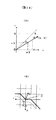
図1には、このような従来の部品認識方法が図示されている。図1(A)はBGA(ボール・グリッド・アレイ)を底面1、すなわち電極側から反射光撮像したものであり、複数のボール電極1a、1b、1c、……が撮像されている。また、(B)はコネクタ、PLCC等リード部品を同条件で撮像したものであり、基礎2に取り付けられたリード2a、2b、2c、……が撮像されている。入力画像は濃淡画像でありXY座標系で画素の位置をあらわすものとする。部品の電極パターンと寸法はあらかじめわかっているから、吸着ノズルの吸着位置のずれと吸着角度のずれを勘案して図で点線1’、2’で示すように、画像内に電極集合の存在範囲(ウィンドウ)を設定し、この範囲で画像へのアクセスを行ない画像処理の高速化を計るのが一般的である。
【0004】
図1(A)は、存在範囲1’の中で水平方向に画像を走査している。走査によって得られた画素の値、すなわち明度をZ軸であらわせば図1(C)の明度グラフが得られる。図1(C)のa、b、cは、それぞれ(A)の画像の走査線a、b、cに対応している。グラフの山の周期Tが電極間距離に等しいことから、走査線cでは電極の列を走査していることが理解できる。図1(A)の電極1aのX座標は、(C)の走査線bのピーク座標であり(x0)、またそのY座標は走査線bとcの間にあることから、両者のY座標を補間することにより求めることができる(y0)。他のボール電極の座標も同様に順次求めて行く。なお、走査する方向は、水平方向走査の他に、垂直方向走査、45度方向走査も加えて位置の信頼性を高めた実施形態もある。
【0005】
図1(B)のリード部品の場合には、走査の結果、電極間距離と同じ周期のリード形状に対応した波形が得られるから、BGAのときと同様な処理を行なえば、リード2a、2b、2c等の先端座標を求めることができる。
【0006】
【発明が解決しようとする課題】
しかしながら、従来の部品認識では、走査線が出力する明度値に依存するため認識対象とする部品の種類によっては認識が困難ないし不可能なものがある。図2には、その例が示されており、(A)はBGA部品3であって、外縁3aがあり、偽電極3bがあり、基礎3cは雑音で汚れ、構造物3dがあり、更に配線3eが走っている。このBGAを撮像すると、それらの明度は、真の対象電極より高いときさえあるので、従来方式で走査した場合には、電極以外の構造を波形として出力するため認識は不可能である。
【0007】
図2(B)は、コネクタ等によく見られるリード部品であり、基礎4には段差構造4aがあり、また止め金具4bが取り付けられている。従って、このリード部品の撮像画面では、これらの段差ないし止め金具の明度が対象電極より高い場合があるので、従来方式で走査した場合、まず上段電極では止め金具4bを取り込んでしまうから、これが真のリードかどうかの判定が困難になる。また下段電極では、段差4aの映像が一様でないため真のリードかどうかの判定が困難である。
【0008】
図2(C)は、(A)と同様BGA部品5である。電極5aだけ映って好条件にもかかわらず従来方式では認識が困難である。なぜなら電極が十字型に並んでいるから水平、垂直、45°、どの方向に走査しても最初の検出波形の山が1個しかないので(45°の場合も部品は普通傾いて映っているから1個になる)、周期の確定を前提とする処理ができないからである。従って、図2(C)のような部品を位置決めするには、その電極パターンに特化した画像処理を行なわなければならないのが、実状である。また画像の走査を行うので、画像全域もしくはその一部の全域の画素数に比例した処理時間がかかるのも難点で、処理時間が大きく、部品搭載のタクト・タイムの点で問題である。
【0009】
このように従来方式では、認識が困難ないし不可能な部品があり、認識精度が劣化する、認識精度を上げるためには、照明・撮像の条件が厳しく機器のコストが上昇する、画像処理速度が遅い、など種々の問題があった。
【0010】
本発明は、上記従来の問題点を解決するためになされたもので、所定配列の電極パターンを有する部品を精度良く認識でき、照明条件が緩く、しかも高速な画像処理が可能な部品認識方法およびその装置を提供することをその課題としている。
【0011】
【課題を解決するための手段】
本発明は、上述した課題を解決するために、所定配列の電極群でなる電極パターンを有する部品を撮像して電極の位置を認識する部品認識方法において、撮像された部品の画像を所定の角から電極1個分に対応する大きさの小窓で掃引して、物理座標上で電極の抽出を行ない、抽出された電極を原点とし、隣り合う電極間の距離を1とする有界の原始地図座標でなる論理座標系を作成し、抽出された電極の論理座標から前記電極パターンを用いて予測される、未抽出の次の電極の論理座標に対応する物理座標上の近傍一定領域に電極1個分に対応する大きさの小窓を設定して、順次電極群の電極パターン並びに各電極の物理座標を求め、求められた電極パターンと前記所定配列の電極パターンとを前記論理座標系上で重ねあわせてずらしながら照合し、両パターンの不一致が最小になる照合結果に基づき求めた前記所定配列の電極パターンの電極画像の論理座標から、この電極パターンの論理座標に対応する求められた電極パターンの各電極の物理座標を求める構成を採用した。
【0012】
また、本発明では、所定配列の電極群でなる電極パターンを有する部品を撮像して電極の位置を認識する部品認識装置において、撮像された部品の画像を所定の角から電極1個分に対応する大きさの小窓で掃引する手段と、掃引された電極1個分に対応する大きさの小窓を介して、物理座標上で電極の抽出を行なう手段と、抽出された電極を原点とし、隣り合う電極間の距離を1とする有界の原始地図座標でなる論理座標系を作成する手段と、抽出された電極の論理座標から前記電極パターンを用いて予測される、未抽出の次の電極の論理座標に対応する物理座標上の近傍一定領域に電極1個分に対応する大きさの小窓を設定する手段と、順次電極群の電極パターン並びに各電極の物理座標を求める手段と、求められた電極パターンと前記所定配列の電極パターンとを前記論理座標系上で重ねあわせてずらしながら照合する手段と、両パターンの不一致が最小になる照合結果に基づき求めた前記所定配列の電極パターンの電極画像の論理座標から、この電極パターンの論理座標に対応する求められた電極パターンの各電極の物理座標を求める手段と、を有する構成を採用している。
【0013】
本発明では、所定配列の電極パターンを有する部品が撮像され、部品の画像を所定の角から小窓で掃引して種電極が抽出される。種電極が検出されると、これを原点にして電極地図座標系H0V0が作成され、周辺電極が観測される状態になる。この状態では、すでに抽出された電極ないし電極群から予測される領域に小窓が設定され、順次電極が抽出されていく。このように抽出された電極のパターン並びにその電極の座標が求められ、抽出された電極パターンと所定配列の電極パターン(論理ないし定義電極パターン)とが重ねて照合され、位置決めが行われる。両パターンの不一致が最も少なくなったときに、すなわち両パターンが最もよく一致するとき、抽出電極の座標値から所定配列の電極パターンの電極の画像座標が決定される。このような構成では、電極の抽出が高速に行われ、しかも抽出された電極パターンと所定配列の電極パターンとが重ねて照合され、位置決めが行われるので、正確な電極の座標値を求めることができる。
【0014】
【発明の実施の形態】
以下、図面に示す実施の形態に基づいて本発明を詳細に説明する。
【0015】
<全体の構成>
図3は、本発明の一実施形態に係わる部品認識装置のブロック構成図であり、画像記憶部10は、照明光源11、11’で照明された認識対象部品12をテレビカメラ(CCDカメラ)13で撮像して得られる部品の濃淡画像を記憶する手段である。照合方向決定部14は、認識対象部品12の電極パターンから認識に有利な角を決める手段であり、候補電極決定部15は、電極パターンの角近傍の電極を選び位置決めの候補とする手段である。
【0016】
不一致許容数決定部16は、電極パターンとその角をもとに位置決めの信頼性を得るための上限値、すなわち不一致許容数を決定する手段であり、探索領域縮小部17は、電極パターンとその角をもとに画像の探索領域をさらに小さくする手段である。また、種電極探索部18は、画像に浮かぶ電極の中から指定角近傍の任意の電極を探し出す手段であり、座標予測部19は、既に抽出された電極群の論理座標と物理座標から、指定された論理座標の電極の物理座標を予測する手段である。
【0017】
また、ボール小窓発生部20はBGAの部品認識のとき作動し、電極の中心予測領域を覆う抽出用の小窓を発生する手段であり、リード小窓発生部21はリード部品の認識のとき作動し、電極の先端予測領域を覆う抽出用の小窓を発生する手段である。更に、三角点発生部22は抽出電極群の望ましい格子の基準点、すなわち測量用の三角点を発生する手段であり、偽電極排除部23は抽出した電極を過去に溯って調べ偽電極を排除する手段であり、電極位置決め部24は抽出される電極のパターンから認識対象部品の画像座標を最終的に確定する手段である。
【0018】
小窓ボール抽出部25はBGA部品の認識のとき作動し、画像内に置かれた窓を通し実際に電極を抽出する手段であり、小窓リード抽出部26はリード部品の認識のとき作動し、画像内に置かれた窓を通し実際に電極を抽出する手段である。
【0019】
また、角三角掃引部27は矩形領域を三角形状に掃引する論理座標を生成する手段、角四角掃引部28は矩形領域を長方形状に掃引する論理座標を生成する手段、らせん掃引部29は矩形領域をらせん形状に掃引する論理座標を生成する手段である。
【0020】
制御部30は各部の制御を行なう。
【0021】
以下に、図4の全体の流れを示すフローチャートに従って、本発明の各処理を詳細に説明する。
【0022】
部品の電極パターンは、格子状に配列された縦M個横N個の矩形仮想電極空間の全体または矩形部分空間であり、部品は仮想電極空間の少なくともひとつの角を共有しかつ少なくとも1個の実電極を持たねばならない。リード部品はM=1に相当するので、例えば、図2(E)に示したようなリード部品7の認識は、図2(D)のBGA部品6のM=1の認識と全く同じ手順で認識される。従って、以下では、縦M個横N個のBGAを部品例にして説明が行なわれる。
【0023】
<照合方向決定>
まず、ステップS20において照合方向決定部14による照合方向が決定される。各部品の電極は所定配列の電極パターンを形成しており、部品データなどから図6に示したような電極パターン(入力時の論理ないし定義電極パターン)を作成することができる。このような所定配列の論理電極パターンはPQ座標系で表され、照合方向決定部14は、この電極パターンからその重心を求め、認識に有利な角を決定する。図6の電極パターンの場合、まずP軸のパターン重心座標Gp、Q軸のパターン重心座標Gq、を次の式で求める。
【0024】
Gp = (Σ(原点からの軸距離(i)×Q方向の実電極数))/実電極数
Gq = (Σ(原点からの軸距離(j)×P方向の実電極数))/実電極数
図6では、
Gp=(0×3+1×4+2×4+3×3+4×3)/17 = 1.94、
Gq=(0×3+1×4+2×5+3×5)/17 = 1.71となる。パターンの中心は(2,1.5)であるから重心Gが左上に位置することがわかる。これから照合座標系hvを図6の向きにとり実際入力パターンをhvの向きに整列して書き換えたパターンを用意する。
【0025】
各hv軸の方向は、重心の位置に従って図8に示したような向きになる。図8(A)〜(D)はそれぞれ右上、左上、左下、右下にそれぞれ重心がある場合のh軸v軸の向きが示されている。
【0026】
図7はリード部品の場合のhv座標の取り方を示す。図7(A)は入力パターンのP座標の終端寄りに重心があるのでh軸は図の向きにとる。このとき仮想的v軸を図の向きにとる。望ましい走査線の動きは図の点線で示す向きであるから実際に画像座標系XYと対応させるときは図8(D)を使う。ただしこのときh軸とv軸を交換する。一方図7(B)に示すように、P軸の原点寄りに重心がある場合には、h軸は図の向きにとる。このときも仮想的v軸を図の向きにとる。望ましい走査線の動きは図の実線で示す向きであるから実際に画像座標系XYと対応させるときは図8(C)を使う。リード部品の認識の場合、このようにリードの向き(例は下向き)に対して座標系が2個必要となり従って実装現場での4方向の向きに対して4×2=8種類の座標変換を用意する。
【0027】
図17の定義電極パターンの場合には、7個の電極があり、領域A、B、Cには電極がないものとする。照合方法決定部14により右上の電極40を位置決めの核とすることが決まり、図18の照合座標系(hv)が張られる。hv座標系は論理座標系であり、座標の中身は1=実電極、0=空電極の2値である。矢印で示したように外側に0を配置して4×4の大きさにしておくと照合の速度を上げることができる。
【0028】
このように、照合方向の決定により認識に最も有利な角が決定され、照合座標系hvに座標変換を行うことができる。
【0029】
<候補電極決定>
次に図4のステップS21に示したように、候補電極決定部15により候補電極が決定される。候補電極決定部15は、電極パターンの角近傍の電極を選び位置決めの候補とする手段である。候補電極は、例えば、図9(A)に図示したような角三角掃引で生成される。角三角掃引の場合、最初の出力は(0、0)以降矢印の向きに原点から遠ざかりながら途中の格子座標を発生する。これにより、図10(A)に示したような電極パターンの場合、候補電極C1〜C5が生成される。候補電極の数は比較的小さい定数(たとえば5)で十分である。なぜなら確率の理論によると電極が小窓で抽出される確率をPとしたとき、N個の電極すべてが抽出されない確率は(1−P)のN乗であり、仮にP=0.9、N=5としてもそれは10のマイナス5乗であるからである。
【0030】
図10(A)はある電極パターンの候補の選出順序をしめすものであり、それらは同図に見るとおり角三角掃引を反時計回りに行なうことによって得られる。一方、図10(A)の電極パターンでは候補電極C6が必要である。これを得るために今度は同じ角三角掃引を時計回りに発生すればよいことが判る。これには反時計回りのときのIJを交換して図10(A)に貼り付けることで容易に達成できる(時計回りの掃引時に得られる5個目の電極がC6である)。
【0031】
このような候補電極C6を必要とする理由は、図10(B)から理解できる。図10(B)において部品が実線36でなく点線36’で図示したように傾きをもって吸着されたとき、電極C5より電極C6のほうが先に抽出されるから処理が少しでも早くなるからである。もう一つの理由は、仮に図10(A)の例で、電極C1〜C4がなく、かつ電極C5とC6間に多くの電極がある部品である場合、図10(B)で実線36に示すような吸着状態のときはC5よりの候補群だけが、そして一方点線36’のときはC6よりの候補群だけが抽出の対象となるからである。
【0032】
図17(図18)の電極パターンの例では、候補電極決定手段により候補者(電極)C1〜C5が決まる。各候補者の中身はその論理座標である。たとえばC1=(2、2)。
【0033】
<不一致許容数決定>
また、ステップS22において、不一致許容数決定部16により電極パターンとそのひとつの角をもとに位置決めの確認を得るための上限値、すなわち不一致許容数(非負整数e)が決定される。不一致許容数とは、ある候補電極が自己の周辺にe以下の不一致数を観測したとき他の候補電極は必ずeより大きい値をとるような数であり、電極パターンの照合時、不一致許容数内にすることにより電極パターンの位置決めの信頼性を高めるために用いられる。不一致許容数決定部16は、その不一致許容数を決定する手段であり、図11にその処理の流れが図示されている。
【0034】
まず、ステップS40において、抽出率と誤読率から不一致許容数lim1が求められる。例えば、電極が小窓の中にあるときの抽出確率をP(たとえば0.95)、電極が小窓の中にないとき誤って他のものを抽出する確率をQ(たとえば0.05)とすれば、
lim1=(1−P)×電極数+Q×仮想電極外周個数
で表される。たとえば、図17の例では、
lim1=(1−0.95)×7+0.05×8=0(個)となる。但し、第1項と第2項のそれぞれで整数まるめが行われている。
【0035】
次のステップS41で、仮想電極の総数を越えるような正数を識別距離としてlim2にセットする。識別距離lim2は電極パターン固有の値であり、0以上の数である。直感的にいえば、2次元に広がる有界の電極パターンがあるとき、同じものを上から被せたとき同じ位置に被せれば上と下の不一致は勿論0個であるが、ひとつでもずらせば不一致数(>0)が観測される。これを候補電極の位置だけ繰り返したときのその最小値をkとする(k>0)。実際に観測される不一致数は真のとき0個、偽のときk個以上であるからlim2=k−1とすればこれは両者を識別できる最大の数であり工業上都合が良い。
【0036】
図12には図17の電極パターンに対するkの求め方を示している。縦の列は、座標系HV原点の位置であり候補電極C1〜C5で示す。横の列は観測する候補電極C1〜C5である。図12の表の値は観測する候補電極がHV座標の原点であると仮定した場合の不一致の観測数の最小値である。時間は上から下に、また左から右に流れている。εはそのときの最小値を越えたことを示す。
【0037】
たとえば、最初の最小値10はHV原点が電極C1のとき電極C2が観測する不一致数である。これは、次のようにして求まる。図18において、この4×4の2値パターンを右上角▲1▼'の電極(その2値は0)から、図9(B)に示す角四角掃引により電極パターン全域にわたって取り出す(▲1▼'、▲2▼'、▲3▼'、....)。電極が取り出されるごとに、電極C1を原点とした場合と(真の原点)、電極C2を原点とした場合の各電極についてその2値が一致しているか、不一致であるかを調べる。
【0038】
まず電極▲1▼'のとき、電極C2からの変位は(2、1)であり、その2値は0(空電極)である。一方、真の原点の電極C1からの変位(2、1)は、パターン空間の正方向の外であるから2値は0である。従って、電極▲1▼'は、電極C1を原点にしても、電極C2を原点にしても同じ2値(=0)となり、両者は一致する。同様に、電極▲2▼'のときも、各2値は0となり一致する。
【0039】
次に電極▲3▼'のときは、2値は1であり、電極C2を原点とすると、電極C2からの変位は(1、0)である。真の原点C1からの同じ変位量の位置は電極▲4▼'が占めているので、その2値は0である。従って、電極C2を原点とすると、電極▲3▼'は実電極(=1)として観測され、また真の原点C1からは空電極(=0)として観測されるので、最初の不一致が発生する。
【0040】
次の電極▲4▼'、▲5▼'では、いずれも2値は0であり、不一致はない。次の電極▲6▼'は自分自身であるからスキップする。次の電極▲7▼'のときは、その2値は0であり、電極C2を原点としたときの変位は、変位(0、−1)である。真の原点C1からの同変位は電極▲8▼'のところであり、その2値は1である。従って、不一致であり、不一致数は2となる。次の電極▲8▼'では、同様に不一致が発生し、不一致数は3となる。以下同様にパターン全域で繰り返す。さらに図17の領域ABCが空であるから図18において、v軸のすぐ左隣(h=−1)の列のパターン値(すべて0)とh軸のすぐ下隣(v=−1)の列のパターン値(すべて0)についても同様に繰り返す(ステップS42)。以上の結果、観測される不一致数は10であり、現在の最小値となる。
【0041】
図12において、次に電極C3を原点として、上記と同様な処理を行い、各電極▲1▼'、▲2▼'、▲3▼'、……ごとに、観測した不一致数を求める。このときは6個の不一致が観測される。これは現在の最小値10より小さいので6に置き換えられる。以下同様に続けると電極C4を原点としたときの不一致数5が最小値のまま表が埋められる。従って、求める不一致の最小値はk=5である。以上は、図11のステップS43、S44の処理に対応し、不一致数がlim2より小さいとときには、lim2はその数で書き換えられる(ステップS44)。
【0042】
注意すべきは図17の電極パターンの場合、領域A、B、Cのどれかが空でないときである。たとえばA、B、Cがすべて空でない、言い換えれば、あるかないか不明のときはkの値は極端に減少する。たとえば図17ではk=1となる。この値は図12の(縦C4,横C1)の位置がとる値となる。なお図13にみられる空のない1次元電極列は点線の左側が空のときk=2、不明のときk=1であり長さに無関係である。ちなみに図1のパターンのABCが不明のとき、k=17である。
【0043】
以上のようにして求められた二つの要求値lim1,lim2に対して、ステップS45でlim2を1減算し、ステップS46で不一致許容数e = MIN{ lim1,lim2}とする。図17の電極パターンの場合、e=0となる。
【0044】
このように、位置決めの確証を得るための不一致許容数が決定される。
【0045】
<探索領域縮小>
次に、図4のステップS23において探索領域縮小部17により電極パターンとそのひとつの角から画像の探索領域をさらに小さくできる。ノズルの吸着範囲から探索範囲は決まっているが、電極パターンの配置からそれを更に狭めることができ、それにより位置決めの処理時間を短縮することができる。
【0046】
図14には、探索領域縮小が行われる様子が、また図15には、その流れ図が図示されている。図14において、角三角座標系ijが示されており、また照合座標系hvが設定されている。まず、ステップS50において、hv座標系右上角の電極から始めて、その中の電極がすべて空である三角形の空虚領域38の深さを求める。この電極パターンの空虚三角形の深さを知るには、撮像された電極パターンの右上から図9(A)の角三角掃引を行えばよい。最初に見つかった電極(=1)の座標(i,j)の角からの軸方向の変位δがわかる。これより図14に示すように角からの軸変位δ−1に開始探索線を設ければよい。
【0047】
一方左下の領域の縮小については、空虚がどんなに深くてもパターンの左下角からの軸変位η=MIN{M−1,N−1}までには実電極があることになっていることを前提にすれば、図14に示すように左下角からの軸変位η−1に最終探索線を設ければよい。
【0048】
なお、図17の電極パターンの場合パターンが小さいため縮小はなされない。
【0049】
<画像取り込み>
続いて、ステップS24において部品の画像の取り込みが行われる。部品は、テレビカメラ13により撮像され、画像記憶部10に記憶される。本発明は、部品の撮像を行うとき、電極数が多ければ全部の電極が映っていなくてもよいし、電極以外のものが映っていてもよいが、部品の認識対象電極のほとんどが映っていることが、前提になる。図2の各部品は、いずれもこの前提を満たしており本発明により高い精度で認識できる部品である。
【0050】
<種電極探索>
続いて、図4のステップS25、S26において種電極探索部18により種電極が探索される。この種電極は、ステップS24で取り込まれた画像に対して照合方向決定部で決定された角から斜め探索が行われ最初に抽出される電極のことである。
【0051】
図22(A)はボール電極のときの種電極の探索を、また図22(B)はリード電極のときの種電極の探索の状態を示している。いずれの場合も角から三角形状に探索範囲を広げることを特徴とする。この位置決めには図9(A)の角三角掃引が使われる。図22(A)において、小窓と小窓の軸距離Δは、Δ = (4/3)ρとするのが適当である。ただしρは、後述する小窓のボール抽出能力と呼ばれる半径である(図24(A))。図22(A)には、小窓44を角三角掃引により掃引することにより種電極(網点の電極)45が抽出される状態が図示されている。
【0052】
一方、図22(B)においては、小窓と小窓の軸距離は、ピッチ方向ΔPとリード方向ΔLに分かれる。ΔP=(4/3)P、ΔL=(4/3)L、とするのが適当である。ただしP、Lは、後述する小窓のリード抽出能力と呼ばれる長さである(図26(A))。図22(B)には、小窓46を角三角掃引により掃引することにより種電極(網点の電極)47が抽出される状態が図示されている。
【0053】
図5の状態図では、領域33の角33aから三角掃引されて種電極32が探索された状態が示されている。また、図19の例では、探索領域の右上角から図のように、位置を三角形に広げながらボール電極の抽出が行われる。小窓が41の位置にきたときに種電極43が抽出されている。
【0054】
<電極地図座標作成>
種電極が探索されると、図4のステップS27に進み、電極地図が作成され、三角測量網が作成され、周辺電極観測状態となる(ステップS27、図5の状態S2)。電極地図は、図5、図20に示したように、抽出された種電極を原点として原始電極地図座標系(H0V0)を張ることにより作成される。この座標系H0V0は論理座標系であって、上限と下限を有し、座標の中身は抽出電極の画像座標、直径(幅)、明度、面積、..等である。図19において種電極43の画像座標は(x1、y1)である。ちなみにボール電極の中心座標とリード電極の先端座標は図16の細粒座標系で示される。細粒座標系は図16の太線48a〜48dで示す画素格子を分割した座標である。図では8分割している。細粒座標系は画像座標系と原点を共有しているので、以降煩わしさを避けるため画像座標系の値として表記する。
【0055】
原始地図座標系は、上述したように上限と下限を有し、図19においてHS、VSはそれぞれ探索範囲X軸Y軸のボール個数換算値として、同個数変位ΔH、ΔVが図から判るので、原始地図座標系H0V0の上限は(ΔH、ΔV)、下限は(ΔH−HS+1,ΔV−VS+1)となる。原始電極地図座標系が有界であることは処理の高速化に欠かせない特長である。
【0056】
次に図20において原始電極地図座標系と原点を共有する(ただの)電極地図座標系(HV)を生成する。これは実体のない仮想の座標系であり原始電極地図座標系とは結合ベクトルで結ばれている。今はそのベクトルは(0,0)である。
【0057】
種電極が抽出された後は、図20原始電極地図座標系の原点の負方向近傍一定領域に対して電極の探索が行われる。この大きさは定数でよくたとえば例では近傍半径=4である。図20では、5×5=25個が探索されている。このときの電極の探索順序は重要である。図9(B)の角四角掃引と名づける座標の発生による掃引による探索順序が使われる。この掃引の最初の出力は(0、0)以降矢印の向きに原点から遠ざかりながら途中の格子座標を発生する。これを図20のIJで示す向きに対応させる。
【0058】
<座標予測>
種電極が抽出された後は、周辺の電極が抽出されるが、その電極抽出は座標予測部19により予測された領域に小窓を設定することより行われる。そのために、座標予測部19は既に抽出された電極群の論理座標と物理座標から、指定された論理座標の電極の物理座標を予測し、予測領域を設定する。この状態が図23(A)、(B)に図示されている。
【0059】
図23(A)は、HV座標系が張られたときに既に存在しているときの電極が1個の場合である。この状況は種電極が抽出された直後にできる。いま既存電極の論理座標を(h1、v1)、予測電極のそれを(h、v)とすれば論理距離の差分(h−h1,v−v1)の各成分にボール間距離(ΔH、ΔV)を乗ずればこれは物理(画像)の距離となる。図6に示すようにボール間距離ΔH、ΔVは、その差はわずかであるが、H軸V軸で一般的に異なっている。この物理ベクトルをXYにおけるHVの置かれた90°回転変位で回転する。さらに吸着ノズルの回転ずれ角度の最大値φをもって右回りと左回りに振る。こうしてできた広がりのある領域にさらに本発明が不確実性と呼ぶ距離ε(図には記載していない)を加算して広げれば最終結果がΓで示す予測領域が設定される。不確実性εは予測に余裕を含ませるための値であり、電極の直径に依存するのがよい。たとえばボールの場合はε=(1/3)ボール半径、リードの場合はε=(1/8)リード幅と定める。なおφは表面実装の現場では5°未満である。
【0060】
一方、図23(B)は、既存電極が2個以上の場合である。この状況は普通の状況である。いま既存電極の論理座標を(h1、v1)、(h2、v2)、予測電極のそれを(h、v)とすれば既存論理距離の差分(h2−h1,v2−v1)の各成分にボール間距離(ΔH、ΔV)を乗ずればこれは物理(画像)の距離となる。同様に差分(h−h1,v−v1)の各成分にボール間距離(ΔH、ΔV)を乗ずる。
【0061】
このふたつのベクトルのなす角度θ(既存から未知の向きに測る、図では負値)がわかり、一方このふたつのベクトルの長さの比(分母は既存、分子は未知、図では1より大)がわかる。既存電極のもつ物理座標の差分を(p2−p1,q2−q1)とすれば(図には記していない)、このベクトルをまずθ回転し、次に長さの比で乗じたのち(逆でもよい)、電極(h1、v1)の物理座標を加算すればこれは予測の中心と呼ばれる座標が生成されたことになる。このあと1点からのときと同様に不確実性距離ε(図には記載していない)を加算して広げれば最終結果がΓで示す予測領域である。なおこのとき長さの比が1より大きいときはその比の分だけ拡大する量も増やす。一方長さの比が1以下のときには加算する量をεとする。図23(B)において、電極(h、v)の予測に使う既存電極は(h、v)の近傍から選ぶ。このとき(h、v)を中心とするらせん状に捜すのが望ましい。
【0062】
このらせん掃引は、図9(C)に示したように、らせん掃引部29により発生され、出発点の座標(i0,j0)が与えられると、最初の出力は(i0+1,j0)以降矢印の向きに原点から遠ざかりながら途中の格子座標を発生する機構である。らせん発生する領域は4つの座標で示される。電極(h、v)の予測においてはそれをらせんの中心におき、電極地図の上限下限をらせん領域に設定すればよい。予測は一般に2個以上の既存電極を使っておこなわれる。
【0063】
なお、後述するように、三角点発生手段により点灯している三角点が2個以上あるときは、その三角点の座標を使って予測を行うことにする。電極(h、v)のもよりの三角点座標がわかるから、上記と同様にその三角点近傍をらせん周回して、点灯三角点2個を捜す。その2個の三角点の保有する電極座標を使って図23(B)と同様に予測する。
【0064】
<小窓発生(ボール小窓)>
上記のように、HV座標系で座標の予測が行なわれると、撮像された電極パターンXY座標系の予測領域を覆う小窓が発生される。そのために、対象部品がボール電極か、リード電極かで、ボール小窓とリード小窓が発生される。ボール小窓は、ボール小窓発生部20により発生され、主にBGA部品の認識のとき発生され、電極の中心予測領域を覆う抽出用の小窓である。図24(A)、(B)に説明図、図25にその流れ図を示す。
【0065】
図24(A)に示すように、発生される小窓には抽出能力ρと呼ぶ半径がある。小窓の中心に半径ρの円53を描いたとき、円内に中心を置く電極ボール像54は必ず抽出される。実施形態ではρ=((√3)/2)×ボール半径と設定されるが、必ずしもこれに限定される必要はない。しかし、実施形態のような値にすると、ボールは、小窓の中心を通る軸による切断長がボール半径以上となり早い段階での合否検査をかけることができるので高速化において有利である。
【0066】
図24(B)は小窓の発生軌跡を示している。まず予測領域の中心に小窓を置き、この小窓から電極ボールの抽出を試みる(図25のステップS60)。図24(B)には、小窓の抽出能力ρの円が細い点線で図示されている。ステップS61で小窓から電極ボールが抽出できたかを判断する。抽出できた場合には、処理を終了する。
【0067】
一方、抽出できなかった場合は、矢印で示す順につぎつぎと小窓を移して抽出を試みる。平面が半径ρの円板で覆われて行く。この場合、小窓は以下に示すようにρを拡大した各段階の能力半径の円周上の位置を順次移動する。電極中心の矩形予測領域(図23(A)、(B))を包み込む最小の円が図24(B)で太い点線(半径R)で示されている。小窓を51に移動した時点でも電極が抽出できなかったとき、ここで抽出が終了してボール電極なしと判定する(ステップS62、S63)。
【0068】
一方、ρが対象被覆半径Rより小さい場合には、以下で示すようにρを拡大して(拡大したρの値をUとして)、小窓の位置を拡大したρの位置に移動してその拡大した段階で同様な処理を繰り返す(ステップS65)。これは、ステップS66でその小窓でボール抽出を行い、ステップS67で抽出できれば処理を終了し、抽出できなければ、Uを有する座標のすべてを実行することによって行われる。
【0069】
この段階でも電極が抽出できない場合には、ステップS68で拡大した能力半径Uが対象被覆半径Rより大きいかを判断し、U>=Rとなっている場合は、抽出を終了してボール電極なしと判定する(ステップS69)。一方、UがまだRより小さい場合には、まだρを拡大して上位の段階に進めるので(ステップS64)、ステップS70に進み、U>=Rとなるまで処理を繰り返す。この場合、ステップS71で示したように、能力半径Uを以下に示すように拡大して登録し、その拡大した能力半径Uの円周上の小窓からボール抽出を実行する。
【0070】
図24(B)において、位置50にある小窓はρを拡大した第1段階の能力半径の円周上にありその最終円である。位置51にある小窓は第1段階の能力半径をさらに拡大した第2段階の能力半径の円周上にありその最終円である。以下同様に拡大を続けるが現実ほとんどの場合第1段階までの予測で済んでいる。従って本発明を実施するときは4段階まで準備しておけば十分である。実施形態では下記の表を定数としてもち高速化を測った。
【0071】
第1段階の半径増加比(対ρ) 0.732、
第2段階の半径増加比(対ρ) 0.775、
第3段階の半径増加比(対ρ) 0.819、
第4段階の半径増加比(対ρ) 0.866、
上記例において第1段階の半径増加比は、半径1の円周上に並ぶ等間隔6個の半径1の円を想定すると、隣り合う円同士の交点が能力の拡大点であるから、予測中心と交点の距離=2×(√3)/2=(√3)からもとの1を引いた値(√3)−1から得られる近似値となっている。また、第4段階の半径増加比は、図24(B)に示したように位置52にある小窓で示す第3段階のさらに外側にできるから直線上に中心を置いて並ぶ間隔1、半径1の円群とみなすことができ、隣り合う円同士の交点が能力の拡大点であるから、直線と交点の距離=(√3)/2から得られる近似値になっている。第2および第3段階の半径増加比の値は第1および第4段階での値をそれぞれ内分したものである。
【0072】
このようなプロセスで小窓を順次発生させ、予測領域にボール電極があるかどうかを検出することができる。
【0073】
<小窓発生(リード小窓)>
以上は、BGA部品のように認識対象がボール状電極であったが、リード部品の場合には、円形の小窓ではなく、リード電極の先端予測領域を覆う抽出用の小窓がリード小窓発生部21により順次発生される。図26(A)、(B)にその状態が説明されており、また図27にその処理の流れが図示されている。
【0074】
図26(A)に示したように、小窓には抽出能力と呼ぶ領域60がある。図26(A)では2P×2Lの小領域である。この領域にその先端を置くリード像61は必ず抽出される。実施形態ではリード形状に応じて領域の大きさを変えている。
【0075】
図26(B)は小窓の抽出能力の軌跡を示している。まずステップS80に示したように、予測の中心が小窓の抽出能力の中心となるように小窓を位置決めしてリード抽出を実行する。従って小窓自身の中心座標はリード方向に図26(A)のPcenterずれた位置にある。図26(B)で抽出能力ピッチ長さ2P、同リード長さ2Lの領域が点線で示されている。
【0076】
図27のステップS81でリード電極が抽出されれば、処理を終了し、抽出できなかった場合は図26(B)の矢印で示す順につぎつぎと小窓を移動して抽出が実行され、平面が2P×2Lの矩形で覆われて行く。リード先端の矩形予測領域が太い点線で示されている。この領域はいずれは有限個の能力で覆われるので、最終段階の能力をかけた時点でも抽出できなかったとき、リード電極なしと判定される(ステップS88)。なお予測領域が小さくて最初の能力に含まれる場合があり、このときは初回で結論がだせることは言うまでもない(ステップS82の肯定)。以下は予測領域が大きくいずれかまたはどちらの方向も能力を超えている場合を想定している。従って、ステップS84で最初の小窓を中心とするらせん旋回の準備をする。
【0077】
図26(B)で予測中心からピッチ方向予測領域の端までの片側区間について考えると、能力の片側個数aはCpitch/2の距離を長さ2Pの線分で多少の被さりを持ちながら覆う問題として扱えば容易である。このようにして個数a個を得る。右がa個なら左もa個である。同様にリード方向も片側個数bを得る。このときaまたはbが0の場合もある(しかしともに0ではない)。能力中心の座標列を出力するには図9(C)に示したらせん掃引を使用する。図26(B)の能力座標列は前記の個数aとbを、imin、imaxともにaとして、jmin、jmaxともにbとして、らせん出力(i,j)を用いれば容易に出力できる。
【0078】
ステップS85、ステップS86のループで、上述したようならせん旋回を行ってらせん出力し、リード抽出を実行する。ステップS87でリードが抽出されれば、処理を終了し、抽出されなければ、ステップS85に戻り、またらせん旋回を終了しても抽出されない場合には、ステップS88でリード電極なしとして処理を終了する。
【0079】
以上のようにして、リード電極の場合も、リード小窓を順次発生させることによりリード電極の予測領域にリード電極があるかを検出することが可能になる。
【0080】
<三角点発生>
なお、上述した座標予測において三角点を発生させることにより座標予測の精度を向上させることできる。三角点は、抽出電極群の望ましい格子の基準点すなわち測量用の三角点であり、三角点発生部22により発生される。図28は三角点測量網の一部分であり、△印が三角点である。三角点は論理座標で管理され隣り合う三角点同士の論理距離は1である(図の太線)。三角点座標系の原点(0、0)は原始電極地図座標系(図20のH0V0)の原点(0、0)と一致している。三角点は原始電極地図座標系の原点電極から起算して、電極の一定個数毎の位置に置く。
【0081】
図28では、4個ごとに三角点が設けてあるがこの数は必然ではない。図28の例では、三角点はその近傍2の距離までの電極の座標を代表している。近傍0距離は三角点自身の電極、近傍1距離は点線で示され、8個の座標がある。近傍2距離はその外側の領域で16個の座標値がある。種電極を得て、図20の原始電極地図座標系を張ったとき、三角点座標系も同時に張られる。原始電極地図座標系に被さるからこの座標系もまた、上にも下にも有界である。このとき原点を除くすべての三角点は初期化されて保有電極はひとつも無い状態である。三角点の原点だけは抽出した種電極の座標としきい値が記録されている。
【0082】
上述した処理により電極の抽出が進行するとともに、電極が一つ検出されるごとにそれを管理する三角点に対して登録作業が行われる。図28は中央の三角点が既に近傍1距離(点線で示す)に4個の電極をかかえていたところに5番目の電極64が近傍1距離に登録されたところである。図28の例では、近傍0距離と近傍1距離にあわせて電極が5個になったとき三角点として点灯すなわち基準点として旗を揚げるようにしているので、電極64の追加により点灯作業を始める。
【0083】
まず、5個の近傍1距離から登録順に先頭と2番目、2番目と3番目、3番目と4番目、4番目と5番目そして5番目と1番目の5組ができるのでこの各組から三角点の座標を予測させる。予測には図23(B)の手段が使われる。これら5組5回の予測座標を記録しておく。一方もし三角点自身が電極の場合、まず自身で1回完了とする。自身を除く4点があるので上と同様に4組4回の予測を行う。
【0084】
一方近傍2距離の電極群についてはもし2個以上あれば、最も遠い2点、図28では電極65と66の2個の電極座標で三角点の予測をする。以上の合計6個の予測座標が得られるから、各軸ごとに6個の座標和を6で割った値として平均座標を得ればこれがすなわち三角点の座標である。
【0085】
このように三角点を発生させることにより座標予測の精度を上げることができる。
【0086】
<電極抽出(ボール電極)>
上述の予測領域に対して画像内に置かれた窓を通して実際の電極が抽出され、座標値が求められる。図29は、小窓ボール抽出部25によりBGA部品を認識するときに行われる処理の流れを示し、図30は、小窓ボール抽出の様子を示す。
【0087】
図30において、70は解剖画像と呼ぶところの、入力画像とは別のメモリに確保した2値をとる小画像である。この画像の大きさは、Rを小窓の半径として、縦横ともに2(R+1)+1=2R+3画素である。2R+3は奇数であるから解剖画像の中心は画素に対応することになる。図30で、各格子点71が解剖画像の画素であり、解剖画像の座標系ΨΩは入力画像系XYと平行である。図22(A)において小窓44の中心画素45がΨΩ座標系の原点に対応する。ボール小窓は論理的には円であるが、図30に示すように解剖画像においては72で示したような経路になる。これは小窓の経路が図31に示すような方向コード0〜7で形成されているからである。小窓の経路は半径Rによって決まるので実施形態では処理範囲のすべてのRについてあらかじめ方向コード列を計算し定数表としてもっておくことにより、小窓72を瞬時に発生させることができる。なお図30で小窓72の外側のすべての解剖画素73は立ち入り禁止のフラグが立っているものとする。
【0088】
ボール抽出は、まずステップS90において小窓内部の濃淡画像を適当なしきい値で2値化して解剖画像に出力する。2値化のためのしきい値は、適当な値を選び、操作者からの指示により決められた値を使うものであればその値とする。一方、自動的にしきい値を求める場合は、次のようにして求める。まず、図30において原点近傍74の数点(たとえば9個)を選び、その対応する(図22(A)の画素45の近傍)入力画素の濃淡値の最大値をaとする。次に、図30で小窓72の経路上の数点(たとえば8個)を選び、その対応する(図22(A)の経路44)入力画素の濃淡値の最小値をbとする。a < C1・b(C1は明度比定数、たとえば1.2)のときは電極無しと判定する。そうでなければしきい値をa、bのM:N内分値とする(たとえばM=3、N=1)。すなわち、しきい値=(Na+Mb)/(M+N)とする。ただしこの値があらかじめ設定されている上下限値を超えたときはその限界値に設定し直す。このようにしきい値を自動計算すれば小窓ごとに適正な値となり照明ムラによる、明度がかたよった画像でも安定した抽出が可能である。
【0089】
解剖画像は、上述のようにして求めたしきい値でΨ軸、Ω軸、小窓経路そして小窓内部の順に2値化することにより行なわれる。Ψ軸の2値化のとき「1」の開始端と終了端をつかんでおき、その長さがボールの半径未満なら電極無しと判定する(図24(A)参照)。Ω軸も同様である。小窓経路の2値化のときは、「1」の数の総数が一定値(たとえば経路画素数の3/5)を超えたら電極無しと判定する。
【0090】
一方、例えば、図30で画素Eを出発点とし、Ψ軸負方向に1画素ずつ進み「1」を検出したら、「1」で囲まれるベクトル(方向コード)列いわゆる島データを出力する。これには公知の方法を用いる。すなわち図32(A)の2値物体80の矢印で示す反時計回り方向コード列を求めるときは、あたかも左手を「1」の壁について離さず前進すればいずれはもとの位置に戻る原理を使う。たとえば図32(A)の円内81の動きを図32(B)に示すと、中心が現在地(画素)である。上に向かう現方向にたいして優先順序を方向7におき、ついで0、1..5の順に調べる。最初に「1」を検出したら(図32(B)では方向3)、それが次の移動方向である。島が一つ生成されたら、Ψ軸上の島を超えた位置からΨ軸の負方向前進を続けて同じことを繰り返す。なおボールの大きさからあらかじめ島の外周長の下限が決まっているものとする。島の開始画素はΨΩ原点まで調べれば十分である。
【0091】
このようにして一般にボール電極がもしあれば1個以上の島データが得られる。ステップS91で前段で出力されたすべての島について以下の処理を繰り返す。ただし途中でボール電極と判定された時点で処理は終了する。
【0092】
いま図30において島Z0〜Z0の島ベクトルデータが取り出されたとする。この島Z0〜Z0で75の部分はボール電極であり、76の部分は配線等の異物である。この島データから図33に示したような、島の構成頂点から選ばれた頂点の表を作成する。このとき、小窓に接触せず、向きが滑らかに変化する区間を選び出してその頂点列を表にする(ステップS92)。例えば、図30においてボール部は小窓と接触し得ないので、小窓との接触頂点77a〜77bは選ばれない。また、向きの変化が90°以上に急な頂点77cも選ばれない。ただし左向き90°の頂点77dは選ばれる。このようにして得られた頂点の座標は、図33において頂点番号を付して頂点座標のところに記録される。なお頂点座標は、ΨΩ座標系の座標である。
【0093】
次に、ステップS93において、図33の表に、濃度勾配ベクトルを記録し、またそのベクトルの8方向分類コードを割り付ける。島Z0〜Z0勾配ベクトルとは頂点における画像濃度の変化方向を示すベクトルであり、たとえば図30で頂点A1ではベクトルGとなる。このベクトルは、公知の方法で求めることができる。例えば、中心画素の勾配ベクトルを求めるときは、図31で方向コード0〜7にそれぞれベクトル(1、0)(1、1)..(1、−1)を割り当て、そのベクトルと、その濃度変化の積を8方向に総和して得られる。勾配ベクトルは濃度の低いところから高いところに向かいその絶対値は濃度差が高いほど大きい。もし頂点がボール電極の頂点である場合には、その勾配ベクトルは図30に見るとおりほぼボール中心Fに向かうことが確認される。なお、図33において、方向コードとは勾配ベクトルのおよその向きを図31の0〜7の方向に分類したものであり、直径の組を見つけるとき中心的な役割を果たすと同時に、処理時間の大きな短縮に役立つものである。
【0094】
次に、ステップS94において、島の直径第1組を求める。図33の表からまず第1頂点A1を順に移動し、それに正対する相手の頂点B1を表から捜す。頂点B1になるには距離、勾配ベクトル同士のなす角度、..等多くの検査が必要である。
【0095】
同様に、次のステップS95で島の直径第2組を求める。図30で頂点A1の方向コード(図31で右上がりだから方向は1である)を反時計回り90°回転した方向(図31で方向3)を出発方向とし、その方向を持つ頂点を表から捜す。表になければ次善の方向すなわちそれから1単位隔たった方向(図31で、方向2および方向4)、2単位隔たった方向まで続け、その頂点をA2とする。それに正対する相手の頂点B2を同様に表から捜す。頂点B2になるには、(A1、B1)のときと同様の検査が必要であり、それに加えて(A1、B1)との位置と角度に関する検査が必要である。たとえば図30において、点線78は不合格となる。
【0096】
この時点でボール電極と確認できるので、ステップS96において、ボール電極の中心座標を求める。まず直径2組4点それぞれに影座標と呼ぶ座標を生成する。影座標は図30で頂点A1ならS点である。影座標は図16で示される細粒座標であり、2値の頂点軌跡の外側をとりまくしきい値そのものをもつ仮想の座標のことである。例えば、図34(A)において、2値画素Oは「1」、画素P、Rはともに「0」とする。Qはどちらでもよい。いまベクトル(a,b)(a>=b>=0)方向の細粒座標T(μ0,ν0)はまずH点の座標が比例配分で容易に知れるから、P点濃度とR点濃度をH座標で比例配分してH点の濃度(しきい値より低い)が求められる。ところがO点はしきい値より高いので、その中間にちょうどしきい値となる位置が存在する。これがT点である。Tは比例配分で簡単に求まる。図34(A)でa>=b>=0に限定したのは処理を簡素にするためである。すなわち、図34(B)において、O点の影座標を求めるにはGの方向が濃度の高い方向であるから、逆向き(−G)の方向を回転と45°での折り返し操作を施すと図でμνの座標系を貼り付けることができる。図34(A)のT点を求めた後、前の操作の逆をおこなえば図34(B)のT座標が得られる。
【0097】
図30において、×印を付したSの影座標4点をSa1、Sb1、Sa2、Sb2とすればこれらを円周上の点とみなすことができる。Sa1、Sb1の垂直2等分線を求め、Sa2、Sb2の垂直2等分線を求め、その2つの直線同士の交点を求める。これが求めるボール電極の座標F(中心座標)である。
【0098】
続いて、ステップS97で、ボールの平均濃度を求め、ボールの直径を求めておく。
【0099】
<電極抽出(リード電極)>
以上のようにしてボール電極が抽出されるが、リード電極の場合には、小窓リード抽出部26により電極抽出が行われる。図35にその流れが、また図36に小窓リード抽出の様子が図示されている。
【0100】
図36において、91は解剖画像と呼ぶところの、入力画像とは別のメモリに確保した2値をとる小画像である。この画像の大きさは縦は2(Rlead+1)+1=2Rlead+3画素である。ただしRleadは小窓93のリード方向の半径である。また横は2(Rpitch+1)+1=2Rpitch+3画素である。ただしRpitchは小窓のピッチ方向の半径である。ともに奇数であるから解剖画像の中心は画素に対応することになる。図36の各格子点92が解剖画像の画素である。解剖画像の座標系ΨΩは入力画像系XYの90°整数倍(0、1、2、3)回転である(図8参照)。図22(B)において小窓46の中心画素47がΨΩの原点に対応する。なお図36で小窓93の外側のすべての解剖画素94は立ち入り禁止の札(フラグ)が立っているものとする。
【0101】
リード抽出を順に追ってみると、まず、ステップS100で、ステップS90と同様に、小窓内部の濃淡画像を適当なしきい値で2値化して解剖画像に出力する。2値化のためのしきい値は、操作者からの指示により決められた値を使うものであればその値とする。一方、自動計算の指示の場合には以下のようにして求められる。図36の原点近傍95の数点(たとえば9個)を選び、その対応する(図22(B)の画素47の近傍)入力画素の濃淡値の最大値をaとする。次に、図36で小窓93の経路上の数点(たとえば8個)を選び、その対応する(図22(B)の経路46)入力画素の濃淡値の最小値をbとする。a < C1・b(C1は明度比定数、たとえば1.2)のときは電極無しと判定する。そうでなければしきい値をa、bのM:N内分値とする(たとえばM=2、N=1)。すなわち、しきい値=(Na+Mb)/(M+N)とする。ただしこの値があらかじめ設定されている上下限値を超えたときはその限界値に設定し直す。このようにしきい値を自動計算すれば小窓ごとに適正な値となり照明ムラによる、明度がかたよった画像でも安定した抽出が可能である。
【0102】
続いて、Ψ軸、Ω軸、小窓経路そして小窓内部の順に上述のようにして求めたしきい値で2値化する。Ψ軸の2値化のとき「1」の開始端と終了端をつかんでおき、その長さがリードの幅未満なら電極無しと判定する。Ω軸も同様である。次に、図36の画素Eを出発点とし、Ω軸正方向に1画素ずつ進み「1」を見つけたら「1」で囲まれるベクトル(方向コード)列いわゆる島データを出力する。これには小窓ボール抽出で述べた方法を用いる。島が一つ生成されたら、Ω軸上の島を超えた位置からΩ軸の正方向前進を続けて同じことを繰り返す。なおリードの大きさからあらかじめ島の外周長の下限が決まっているものとする。島の開始画素はΨΩ原点付近まで調べれば十分である。
【0103】
このようにして一般にリード電極がもしあれば1個以上の島データが得られる。ステップS101で、前段で出力されたすべての島について以下の処理を繰り返す。ただし途中でリード電極と判定された場合には、処理を終了する。
【0104】
いま、図36において、96をリード電極として島Z0〜Z0が取り出されたとする。ステップS102で、この島のΩ座標最大点Ztopと最小点Zbottomを求め長さを検査をする。続いて、ステップS103で、始点Z0から時計回りに進みZtopに至る経路を生成する。同様に反時計回りも生成する。なお、このとき、操作者からはリード先端の不安定区間長(α)と安定区間長(β)とリード幅(γ)が指示されているとする。また、さきの両経路において、Z0からの高さ(α+β)ラインまでは小窓に接触してはならない。
【0105】
続いて、ステップS104で、Z0からの高さ(α+β)ラインを横断すれば島の幅第1組(A1、B1)が分かり、幅の検査をする。また各点において滑らかに方向が変化しているか検査される。次に、ステップS105で、Z0からの高さαラインを横断することにより幅第2組(A2、B2)が分かり、幅の検査をする。また各点において滑らかに方向が変化しているか検査される。不合格のとき、1上昇した横断線で同じ検査を行う。これを繰り返し(A1、B1)手前までにみつかればよしとする。
【0106】
このようにして、リード電極が確認できたときには、ステップS106で、リードの中心線を求める。まず上述のようにして求めた幅2組4点にそれぞれに影座標を生成する。影座標は小窓ボール抽出と同じものである。図36において、A1ならS点である。×印(S点)の影座標4点をSa1、Sb1、Sa2、Sb2とすれば、リードの中心線97はSa1、Sb1の中点を通り、かつSa2、Sb2の中点を通る。また、Zbottomに影座標Sbを生成し、Sbから、さきのリード中心線97に垂線を降ろし、その垂点が求めるリード電極の先端座標(図36のF点)である。
【0107】
なお、リード電極のときも、ステップS107でリードの平均明度を求め、リードの幅を求めておく。
【0108】
<偽電極排除>
図4の全体の流れに戻れば、上述したように種電極が探索され(ステップS26)、電極地図、三角測量網が作成され(ステップS27)、周辺電極観測状態(ステップS28)となり、この周辺電極観測状態(S2)では、上述したように、電極予測領域に小窓を発生させて電極があるかないかの検出が行われ、周辺電極の抽出が行われる。図5では種電極32の近傍の電極が×印で示したように抽出されている。なお34は偽電極であり、このような偽電極があると、電極の位置予測精度が劣化するので、偽電極排除部23により抽出した電極を過去に溯って調べ偽電極を排除するようにする。
【0109】
例えば、図37(A)において抽出電極100は座標が狂っていて明らかに偽電極(電極もどき)である。実施形態では望ましい格子座標からボール半径を超えて存在する電極を偽電極と判定している。このような電極はその周辺の電極の位置予測を狂わす元凶となるので早いうちに摘出排除せねばならない。また位置決めの照合の不一致回数にも数えられるのでこの意味からも除去が必要である。
【0110】
一方図37(B)の電極101は直径が小さすぎて明らかに偽電極(電極もどき)である。直径以外には明度の低すぎるあるいは高すぎることも偽電極の判定に使われる。この直径(リードの場合は幅,以下断らない)と明度を電極の固有値と呼ぶことにする。実施形態では常時固有値の平均値を管理している。ある電極のどちらかの固有値が、平均値の±40%を超えたとき偽電極と判定している。このような電極は一般に座標も狂っていてその周辺の電極の位置予測を狂わす元凶となるので早いうちに摘出排除せねばならない。また位置決めの照合の不一致回数にも数えられるのでこの意味からも除去が必要である。
【0111】
そこで、図38に示す流れに沿って偽電極の排除が行われる。まず、ステップS110において、座標予測領域から電極の抽出が行われ(ステップS111で拒否座標群を検査する)、ステップS112で固有値の検査が、またステップS113で座標の格子点の検査が行われる。また、電極が抽出されると、ステップS114において、上述したように電極地図に記入され、三角点に送出され、抽出電極数に1が加算される。
【0112】
最初の抽出電極が偽であることもあるし、それを含めて早いうちに抽出した複数の電極が偽であるかもしれない。初期の段階では平均値が存在し得ないので除去することはできない。このような問題は状態遷移図により解決される。図39(A)は固有値の状態遷移図を、また図39(B)は位置の状態遷移図を示している。固有値についてのべると、最初の電極である種電極を得ると状態P1に行く。電極数は1となる。種の固有値(直径/明度)がそれぞれの場所に総和値として書き込まれる。2番目の電極が抽出された場合も、その固有値を足し込むだけである。以下同様に進み、6番目の電極が抽出されると、その固有値を足し込んだあと、その総和を6で割りすなわち平均値をだす。直径の平均値と明度の平均値が公表される。同時に固有値に関する一斉検査を要求して(張り紙をだして)状態をP2に移す。状態P2では電極が入れば平均値を常時更新してもとの状態から動かない。一方偽電極の排除が行われるとその知らせが入り、その電極の固有値分だけ総和から引かれ平均値が更新される。排除後の電極数が依然として6以上あれば状態は変わらないが、もし5になったら(4以下であることはありえない)、状態をP1に移動する。以下は同様の遷移が繰り返される。
【0113】
一方位置の状態遷移図の場合、管理する値はないが電極数が8個未満のときはZ1を続ける。7個から8個に増えるとき一斉検査を要求して(張り紙をだして)状態をZ2に移す。状態Z2では電極が入ればもとの状態から動かない。一方偽電極の排除が行われるとその知らせが入り、排除後の電極数が依然として8以上あれば状態は変わらないが、もし7になったら(6以下であることはありえない)、状態をZ1に移動する。以下は同様の遷移が繰り返される。
【0114】
これだけの単純な動きで偽電極はすべて排除される。すなわち偽電極が排除されるときというのは、P1(Z1)からP2(Z2)に移動するときの一斉検査要求が実行されるときである(これは偽電極がなくなるまで何回でもおこることに注意)。P2(Z2)状態においては新規入力電極が登録されるまえに平均値による審査をうけるので問題無い。
【0115】
上述した流れが、ステップS115〜S119に図示されている。
【0116】
既存の電極が排除されたときと、新規電極が事前審査で不合格になったとき、その座標を図40のXY座標の配列に加える。この配列は拒否座標群と呼ばれる。図5の初期状態において初期化され以降初期化されることはない。すなわち溜まる一方であり画像全域において過去に排除された偽電極が再び抽出されることを防ぐ役目を持つ。なお表面実装の現場において、画像内の偽電極の数は高々20個程度である。そのため図40の矢印で示す容量はこの数程度用意すれば十分である。
【0117】
なお上記の、遷移条件として例示した電極数6または8は必然性の数ではない。
【0118】
<電極位置決め>
図4に戻って、周辺電極観測状態(図5のS2)で、偽電極が発生して電極の喪失があれば空電極を初期化し(ステップS29)、初期(原始)電極地図原点周辺を抽出し(ステップS30)、電極の喪失がなければ原点電極追跡状態S3となる(ステップS31)。原点電極追跡状態では、位置決め成績表が初期化され(ステップS32)、図5に示したように、種電極32を筆頭に近傍何個かの電極に対して順に、あらかじめ決めておいた複数候補電極の誰かであるかどうかの打診がなされ、ある候補に間違いないと判定されれば、位置決め完了状態(S4)に行く。一方、どの候補でもなかった場合種電極32はおそらく偽電極であり状態S1に戻る。また一方、途中偽電極の排除が起こることがある。そのときは直ちにS2に行く。S2では排除された電極34の近傍電極の再調査が行われる。そして再度種電極32(種自身が排除されていることもありうる)の近傍の抽出が行われ(調査の必要なものに限る)偽電極がより少なくなった状態で再びS3に行く。
【0119】
このようにして最終的には状態S3において種電極32の近傍のどれかがある候補者と一致して必ずS4に抜ける。なおS4に行くとき、種電極32は必ずしも真の電極とは限らないことに注意する。
【0120】
状態S3からS4間で行われる電極の位置決め(ステップS32〜S35)を図41の流れを参照して説明する。この流れにおいて、電極位置決め部24(図3)により、抽出された電極のパターンから認識対象部品の電極の画像座標が最終的に確定される。まず、ステップS120で、位置決め成績表を初期化し、不一致許容数をすでに求めてあるe(図4のステップS23)にセットする。
【0121】
図5の状態S3の時点では、初期電極地図座標系H0V0の近傍(種検出直後)もしくは相当広い範囲(偽電極排除後)に抽出電極が分布している。依然として候補電極はH0V0原点の近傍にいるはずであるから、原点近傍の数個が候補電極かどうかを検査すればよい。候補電極は既に見たように角三角形状に展開しているから、その展開にあわせて、初期(原始)電極地図座標系原点より負方向に角三角掃引を行い、その毎回の論理座標に対応する実電極を機械的に取り出して(ステップS121)、座標のオフセット操作により(ただの)電極地図座標系の原点をその実電極にずらし(ステップS122)、各候補者に自分が電極地図座標系原点であると仮定したときの論理予測値(図18に示したような定義電極パターンからの有り/無し)と現実の観測値(図20ないし図21の電極地図座標系の電極の有り/無し)の一致/不一致を調べさせ、その不一致数を位置決め成績表に記録していく(ステップS123)。この記録に際しては、オフセットの回数ごとに不一致数の最小値だけに着目するときわめて高速化できる。eの初期値は前出の不一致許容数である。
【0122】
1回目はこの値を上限に照合検査が行われる。もし生存候補があれば(従ってe以下の不一致を観測した候補者があれば)それらの不一致観測数の最少値を次の回(2回目)の上限としてeを書き換える(ステップS124)。このようにすれば、正しい照合は不一致数最小の照合であるという自然原理に従うと同時に、回を追うごとにeが単調減少するため候補者の死亡が急速に進み、従って高速位置決めが可能となる。
【0123】
なお位置決め時のオフセットの個数は任意で良いが候補者と同数程度にするのが自然である。なお、この位置決め過程においては、電極地図座標系(HV)の、まだ調べられていない論理点に対して、画像からの電極抽出が行なわれる。その順序は、そのときの地図と定義パターンとにより決まり、必ずしも規則的な動きとはならない。
【0124】
図41の流れの中で、ステップS125において不一致許容数以下の値を持つ候補電極が存在したかが判断され、肯定される場合は、成績表から最小値を持つ候補電極を探す。その候補電極の真の画像座標はそのときの電極地図原点電極の画像座標であるので、電極パターンの電極の画像座標が求まり、電極の位置決めが完了する(ステップS126)。一方、ステップS125の判断が否定される場合は、検出した種電極では位置決めができなかったので、抽出された電極数の数を評価し処理を繰り返す(ステップS127)。
【0125】
例えば、入力時の電極パターンが図17の場合、論理電極パターンないし定義電極パターンは図18のようになり、また図21のように電極が抽出されて原始電極地図座標系H0V0に展開している。図21の丸で囲んだ数字の順に(ただの)電極地図座標系HVが原始電極地図座標系H0V0から分離される。図21では2回目の結合ベクトル=(−1、0)の様子を示している。この座標順序は既にみた角三角掃引である。
【0126】
図42には各候補者が毎回の原点分離において自分がHV原点であると仮定した場合に観測する不一致の数が図示されている。*印は許容数(e=0)を超えたため候補者が死んだことを示す。一致/不一致は論理電極パターンの論理値(図18)と観測値(図21のHV座標系)間のものである。図18のIJは既にみた角四角掃引である。最初は結合ベクトル▲1▼=(0、0)である。これは図20の状態であるから図18の候補者C1が原点のとき完全に一致しているのでC1の観測する不一致数は0である。
【0127】
一方候補者C2の立場からは図18のC2に原点をおいてみれば目視でも容易に数えられ、不一致数は10個となる。たとえばC2の右横にはC1があるはずなのに図20HV原点の右横の座標(1、0)の観測結果は空電極であろうからひとつの不一致が計数される。候補者C2は許容数e=0をはるかに超えて不適格になり死亡する。C3〜C5も同様である。
【0128】
次に原点が分離されて▲2▼の位置にきて、結合ベクトル▲2▼=(−1、0)となる。これは図21の状態であるから候補者C2が原点のとき完全に一致しているのでC2の観測する不一致数は0である。逆に候補者C1は死亡する。他の候補者も同様に死亡する。以下同様に結合を▲3▼▲4▼▲5▼▲6▼と試すことにより図42の位置決め成績表が得られる。なお▲5▼は実電極でないため試験からはずしている。
【0129】
今回の位置決め成績表をみると最小値0が存在してどの候補者ももしそれを持てば唯一個所だけである。この状態は、曖昧性のない位置決め状態と呼ばれる。
【0130】
図43は、従来図の説明に用いた図1(A)のBGAを本発明方式で認識した結果である。最初の種電極はC2であった。そのためそれより高いところにあるC1とC3は位置決めの電極が自分に回ってこないため毎回死亡している。他の候補は不一致数ゼロを報告して、正しい認識が完了している。ちなみにこのときの不一致許容数は4であった。
【0131】
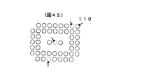
一方、図44は図45のBGA部品を撮像したのち、定義電極パターンとして図1(A)のものをそのまま入力し、本発明方式で認識した結果である。図45において矢印の4個所が定義パターンと食い違いがある。不一致許容数は定義パターンがおなじであるから4で変わらない。実際につかんだ最初の種電極は図45の電極110であった。すなわち回数▲1▼▲2▼..はこの電極が起点である。▲1▼はどの候補でもないから全員死亡、▲2▼は実電極でないから無視、▲3▼以降はそれぞれの候補者がおり、各候補者は等しく不一致数4を報告している。許容不一致数を合格した正しい認識が完了している。なおこの後、実装の現場では操作者にエラーを検出した電極部位の表示をして、判断を委ねることが一般的である。
【0132】
このようにして電極位置決めにより、抽出電極パターンの座標値から認識対象部品の電極パターンの位置、すなわち部品の電極の画像座標を決定することができ、図5の状態S4の位置決め完了状態となる。ここでの処理は本発明とは直接関係がないので説明を省略するが、部品表面実装の現場では得られた電極の形状診断、位置診断のあと電極の画像座標からロボット・アームが行なうべき搭載位置のずれ補正量と角度補正量を出力することになる。
【0133】
<他の実施形態>
上述した実施形態では、電極の明度がその背景より高い場合を例示したが、逆に低い場合(セラミック基礎の半田ボール等)でも効果は全く変わらない。なおそのときは小窓からの電極抽出部だけの変更ですみ、しかも、しきい値に対する大小判断を逆にするだけで済む。
【0134】
また、種電極の探索に関して、角四角掃引にすると、多少能率が落ちるが効果はほとんど変わらない。さらに、候補電極の選定に関して、角四角掃引にしても、効果は全く変わらない。また、位置決めの原点電極に関して、角四角掃引にしても、効果は全く変わらない。
【0135】
【発明の効果】
以上説明したように、本発明によれば以下の効果が得られる。
【0136】
a)位置決めを推進する力は画像から抽出される電極の有り無しの情報だけである。もし電極以外のものを間違えて電極として抽出しても、あとで偽電極の排除により捨てられるので問題ない。また仮に本物と区別のつかない、従って排除できない偽電極が混入しても、不一致許容数の範囲なら誤りのない位置決めが可能である。従って、現市場の格子配列電極部品のほとんどが認識可能である。従って、ほとんどすべての部品が高精度で認識できる、という効果が得られる。
【0137】
b)電極は小窓から抽出され、小窓の座標は三角点を使った座標予測から発生する。そのため歪んだ画像でも歪んだなりに予測は正確である。また小窓の2値化のしきい値は小窓毎に設定される。そのため照明ムラに強く、雑音に強く、また全体に暗いもしくは明るい画像でも抽出可能である。以上のことからカメラや照明の品質に対する要求を少なくすることが出来、廉価の機器で構成することができる。
【0138】
c)画像データにアクセスする量が少なく、最初の種電極を見つけるまではその面積に比例した時間がかかるがその量はわずかである。種電極が検出された後は、論理的判断の時間と、予測された局所領域からの電極抽出の時間の和であり、これはほぼ電極数に比例した時間となり、画像サイズに比例する従来方式と比べると、本発明の方式のほうが処理が原理的に早くなる。
【0139】
d)本発明の方式が適用出来るのは、部品の角を含む画像であって、部品全体が映っている必要はない。部分認識とは大きな部品を複数回分割撮影して成る、部品の部分画像からその一部の電極群を位置決めすることであるが、本方式により原理的に部分認識が可能になる。
【0140】
e)三角点の働きによる効果が得られる。三角点はその仮想電極の格子座標をもっており、三角点から予測した座標は本来あるべき電極座標である。これと実際に抽出される座標には一般に誤差があるので、全電極にわたって統計処理すれば、誤差の標準偏差が得られ、誤差長の大きい異常電極を判定することが容易である。とくに歪んだ画像でも歪んだなりに位置の診断ができることが本発明の効果である。
【図面の簡単な説明】
【図1】従来の部品認識の方法を説明した説明図である。
【図2】認識される電極のパターンないし配列を示した説明図である。
【図3】本発明の全体構成を示すブロック図である。
【図4】本発明で行われる処理の全体の流れを示すフローチャート図である。
【図5】本発明の処理の中で現れる種々の状態を示した状態図である。
【図6】電極パターンの重心を求める状態を示した説明図である。
【図7】照合方向の決め方を説明した説明図である。
【図8】照合方向の決め方を説明した説明図である。
【図9】種々の掃引方式を説明した説明図である。
【図10】位置決めの候補電極の選定を説明した説明図である。
【図11】不一致許容数を決定するときの流れを示すフローチャート図である。
【図12】不一致許容数を決定するときに作成される表図である。
【図13】不一致許容数を決定するときに用いられる電極パターンを示したパターン図である。
【図14】電極を探索するとき探索領域が縮小される状態を示した説明図である。
【図15】電極を探索するとき探索領域を縮小する処理の流れを示したフローチャート図である。
【図16】座標値を記述する細粒座標を示した説明図である。
【図17】部品の論理ないし定義電極パターンを示すパターン図である。
【図18】部品の論理ないし定義電極パターンから不一致許容数を決定する状態を説明した説明図である。
【図19】種電極の抽出を説明する説明図である。
【図20】種電極が抽出されたとき作成される原始電極地図座標系を示す説明図である。
【図21】抽出された電極パターンを電極地図座標系で示すパターン図である。
【図22】種電極の抽出を説明する説明図である。
【図23】抽出された電極から他の電極が存在する領域を予測する状態を示した説明図である。
【図24】予測領域にボール小窓を発生させる状態を示した説明図である。
【図25】予測領域にボール小窓を発生させる流れを示したフローチャート図である。
【図26】予測領域にリード小窓を発生させる状態を示した説明図である。
【図27】予測領域にリード小窓を発生させる流れを示したフローチャート図である。
【図28】測量用の三角点を発生させる状態を示した説明図である。
【図29】ボール電極を抽出してその座標値を求める流れを説明したフローチャート図である。
【図30】ボール電極を抽出してその座標値を求める状態を説明した説明図である。
【図31】ボール電極抽出の過程で用いられる方向コードを示すコード図である。
【図32】ボール電極の抽出を説明する説明図である。
【図33】ボール電極を抽出するときに得られる頂点の座標が格納される状態を示した表図である。
【図34】ボール電極の座標を求める状態を示した説明図である。
【図35】リード電極を抽出してその座標値を求める流れを説明したフローチャート図である。
【図36】リード電極を抽出してその座標値を求める状態を説明した説明図である。
【図37】偽電極が抽出された状態を示す説明図である。
【図38】偽電極を排除する流れを示したフローチャート図である。
【図39】偽電極排除の過程を説明する説明図である。
【図40】偽電極排除のときに使用される座標図である。
【図41】電極位置決めの流れを示すフローチャート図である。
【図42】電極位置決めのとき用いられる成績表を示した表図である。
【図43】電極位置決めのとき用いられる成績表を示した表図である。
【図44】電極位置決めのとき用いられる成績表を示した表図である。
【図45】電極位置決めを説明する電極パターン図である。
【符号の説明】
12 部品
13 テレビカメラ
14 照合方向決定部
15 候補電極決定部
16 不一致許容数決定部
17 探索領域縮小部
18 種電極探索部
19 座標予測部
20 ボール小窓発生部
21 リード小窓発生部
22 三角点発生部
23 偽電極排除部
24 電極位置決め部
25 小窓ボール抽出部
26 小窓リード抽出部
27 角三角掃引部
28 角四角掃引部
29 らせん掃引部[0001]
BACKGROUND OF THE INVENTION
The present invention relates to a component recognition method and apparatus, and more particularly, to a component recognition method and apparatus capable of positioning an image of a component imaged in an electronic component surface mounting apparatus or the like.
[0002]
[Prior art]
In the surface mounting apparatus for electronic components, the electronic components are supplied from a component supply device (feeder), sucked by a suction nozzle, and mounted on a circuit board. Since the suction nozzle does not always pick up electronic components in the correct posture, the picked-up component is usually imaged by a CCD camera or the like, and the component is recognized. Correction, tilt correction, etc. are performed.
[0003]
FIG. 1 shows such a conventional component recognition method. FIG. 1A shows a reflected light image of a BGA (ball grid array) from the
[0004]
In FIG. 1A, an image is scanned in the horizontal direction within the
[0005]
In the case of the lead component shown in FIG. 1B, a waveform corresponding to the lead shape having the same cycle as the distance between the electrodes is obtained as a result of scanning. Therefore, if the same processing as in the case of BGA is performed, the leads 2a, 2b Tip coordinates such as 2c can be obtained.
[0006]
[Problems to be solved by the invention]
However, in conventional component recognition, depending on the brightness value output by the scanning line, there are some components that are difficult or impossible to recognize depending on the type of component to be recognized. An example is shown in FIG. 2, (A) is a
[0007]
FIG. 2B shows a lead component often found in a connector or the like. The
[0008]
FIG. 2C shows the
[0009]
As described above, in the conventional method, there are parts that are difficult or impossible to recognize, the recognition accuracy is deteriorated, and in order to increase the recognition accuracy, the conditions of illumination / imaging are severe and the cost of the equipment is increased, and the image processing speed is increased. There were various problems such as slowness.
[0010]
The present invention has been made to solve the above conventional problems. A part having an electrode pattern of a predetermined arrangement It is an object of the present invention to provide a component recognition method and apparatus capable of accurately recognizing a product, having a gentle illumination condition, and capable of high-speed image processing.
[0011]
[Means for Solving the Problems]
In order to solve the above-described problems, the present invention provides a predetermined array. Consisting of electrodes In a component recognition method for imaging a component having an electrode pattern and recognizing the position of the electrode, the image of the imaged component is changed from a predetermined corner to one electrode. Correspondence Swept with a small window At The pole is extracted and extracted Power Bounded with the pole as the origin and the distance between adjacent electrodes as 1. Consist of primitive map coordinates Create a logical coordinate system and extract Electrode From logical coordinates Using the electrode pattern is expected , Unextracted For one electrode in a certain constant neighborhood on the physical coordinates corresponding to the logical coordinates of the next electrode Correspondence Set a small window of the size you want, and sequentially group of electrode Pattern each The physical coordinates of the electrode are obtained, and the obtained electrode pattern and the electrode pattern of the predetermined array are overlapped on the logical coordinate system. While shifting From the logical coordinates of the electrode image of the electrode pattern of the predetermined arrangement obtained based on the collation result obtained by collating and minimizing the mismatch between both patterns, Electrode pattern Corresponds to logical coordinates For each electrode of the required electrode pattern Physical coordinates Asking The configuration is adopted.
[0012]
In the present invention, the predetermined arrangement Consisting of electrodes In a component recognition apparatus that images a component having an electrode pattern and recognizes the position of the electrode, the image of the captured component is changed from a predetermined corner to one electrode. Correspondence A means of sweeping with a small window of the size to be used, and one swept electrode Correspondence On physical coordinates through a small window At Means to extract the poles, Power Bounded with the pole as the origin and the distance between adjacent electrodes as 1. Consist of primitive map coordinates Means to create a logical coordinate system, and extracted Electrode From logical coordinates Using the electrode pattern is expected , Unextracted For one electrode in a certain constant neighborhood on the physical coordinates corresponding to the logical coordinates of the next electrode Correspondence Means to set a small window of the size, and electrodes in sequence group of electrode Pattern each Means for obtaining physical coordinates of electrodes, and superimposing the obtained electrode pattern and the electrode pattern of the predetermined arrangement on the logical coordinate system While shifting From the logical coordinates of the electrode image of the electrode pattern of the predetermined arrangement obtained based on the matching means and the matching result that minimizes the mismatch between the two patterns, Electrode pattern Corresponds to logical coordinates For each electrode of the required electrode pattern Physical coordinates Asking The structure which has a means to adopt.
[0013]
In the present invention, a part having an electrode pattern of a predetermined arrangement is imaged, and a seed electrode is extracted by sweeping the image of the part from a predetermined corner with a small window. When the seed electrode is detected, the electrode map coordinate system H0V0 is created with this as the origin, and the peripheral electrodes are observed. In this state, a small window is set in a region predicted from the already extracted electrode or electrode group, and electrodes are sequentially extracted. The extracted electrode pattern and the coordinates of the electrode are obtained, and the extracted electrode pattern is collated with a predetermined array of electrode patterns (logic or definition electrode pattern) to perform positioning. When the mismatch between the two patterns is minimized, that is, when the two patterns match best, the image coordinates of the electrodes of the electrode pattern in the predetermined arrangement are determined from the coordinate values of the extracted electrodes. In such a configuration, the electrodes are extracted at high speed, and the extracted electrode pattern and the electrode pattern in a predetermined arrangement are collated and positioned, so that positioning is performed. it can.
[0014]
DETAILED DESCRIPTION OF THE INVENTION
Hereinafter, the present invention will be described in detail based on embodiments shown in the drawings.
[0015]
<Overall configuration>
FIG. 3 is a block diagram of a component recognition apparatus according to an embodiment of the present invention. The
[0016]
The discrepancy allowable
[0017]
The ball
[0018]
The small window
[0019]
Further, the square
[0020]
The
[0021]
Below, according to the flowchart which shows the whole flow of FIG. 4, each process of this invention is demonstrated in detail.
[0022]
The electrode pattern of the part is the whole or a rectangular partial space of M vertical N horizontal virtual electrode spaces arranged in a grid pattern, and the part shares at least one corner of the virtual electrode space and has at least one piece. Must have a real electrode. Since the lead component corresponds to M = 1, for example, the recognition of the
[0023]
<Determination of collation direction>
First, in step S20, the collation direction is determined by the collation direction determination unit 14. The electrode of each component forms an electrode pattern of a predetermined arrangement, and an electrode pattern (logic or definition electrode pattern at the time of input) as shown in FIG. 6 can be created from component data or the like. Such a predetermined arrangement of logic electrode patterns is represented in the PQ coordinate system, and the collation direction determination unit 14 obtains the center of gravity from the electrode pattern and determines an angle that is advantageous for recognition. In the case of the electrode pattern of FIG. 6, first, the pattern centroid coordinates Gp of the P axis and the pattern centroid coordinates Gq of the Q axis are obtained by the following equations.
[0024]
Gp = (Σ (axial distance from origin (i) × number of actual electrodes in Q direction)) / number of actual electrodes
Gq = (Σ (axial distance from origin (j) × number of actual electrodes in P direction)) / number of actual electrodes
In FIG.
Gp = (0 × 3 + 1 × 4 + 2 × 4 + 3 × 3 + 4 × 3) /17=1.94
Gq = (0 × 3 + 1 × 4 + 2 × 5 + 3 × 5) /17=1.71. Since the center of the pattern is (2,1.5), it can be seen that the center of gravity G is located at the upper left. A rewritten pattern is prepared by arranging the collation coordinate system hv in the direction of FIG. 6 and aligning the actual input pattern in the direction of hv.
[0025]
The direction of each hv axis is as shown in FIG. 8 according to the position of the center of gravity. FIGS. 8A to 8D show the directions of the h-axis and v-axis when the centers of gravity are located at the upper right, upper left, lower left, and lower right, respectively.
[0026]
FIG. 7 shows how to take the hv coordinate in the case of a lead component. In FIG. 7A, since the center of gravity is near the end of the P coordinate of the input pattern, the h axis is in the direction shown in the figure. At this time, the virtual v-axis is set in the direction shown in the figure. Since the desirable movement of the scanning line is the direction indicated by the dotted line in the figure, FIG. 8D is used when actually corresponding to the image coordinate system XY. However, at this time, the h-axis and the v-axis are exchanged. On the other hand, as shown in FIG. 7B, when the center of gravity is near the origin of the P-axis, the h-axis is oriented as shown. At this time, the virtual v-axis is set in the direction shown in the figure. Since the desired movement of the scanning line is the direction indicated by the solid line in the figure, FIG. 8C is used to actually correspond to the image coordinate system XY. In the case of lead component recognition, two coordinate systems are required for the lead direction (for example, downward) as described above. Therefore, 4 × 2 = 8 types of coordinate conversion are performed for the four directions at the mounting site. prepare.
[0027]
In the case of the definition electrode pattern shown in FIG. 17, it is assumed that there are seven electrodes and there are no electrodes in the regions A, B, and C. The collation method determination unit 14 determines that the upper
[0028]
Thus, the most advantageous angle for recognition is determined by determining the collation direction, and coordinate transformation can be performed on the collation coordinate system hv.
[0029]
<Candidate electrode decision>
Next, as shown in step S <b> 21 of FIG. 4, candidate electrodes are determined by the candidate electrode determination unit 15. The candidate electrode determination unit 15 is a means for selecting an electrode near the corner of the electrode pattern as a positioning candidate. Candidate electrodes are generated, for example, by angle triangle sweep as illustrated in FIG. In the case of the angular triangle sweep, the first output is (0, 0) and subsequent halfway grid coordinates are generated while moving away from the origin in the direction of the arrow. Thus, candidate electrodes C1 to C5 are generated in the case of the electrode pattern as shown in FIG. A relatively small constant (for example, 5) is sufficient for the number of candidate electrodes. This is because, according to the theory of probability, when the probability that an electrode is extracted by a small window is P, the probability that all N electrodes are not extracted is the Nth power of (1-P), and P = 0.9, N This is because even if = 5, it is 10 to the fifth power.
[0030]
FIG. 10A shows a selection order of candidates for a certain electrode pattern, which can be obtained by performing a triangular triangle sweep counterclockwise as shown in FIG. On the other hand, the candidate electrode C6 is required in the electrode pattern of FIG. In order to obtain this, it can now be seen that the same angular triangular sweep may be generated clockwise. This can be easily achieved by exchanging the IJ in the counterclockwise direction and attaching it to FIG. 10A (the fifth electrode obtained during the clockwise sweep is C6).
[0031]
The reason why such a candidate electrode C6 is required can be understood from FIG. This is because when the part is attracted with an inclination as shown by the dotted line 36 'instead of the
[0032]
In the example of the electrode pattern of FIG. 17 (FIG. 18), candidates (electrodes) C1 to C5 are determined by the candidate electrode determining means. The content of each candidate is its logical coordinates. For example, C1 = (2, 2).
[0033]
<Determination of discrepancy allowable number>
In step S22, the upper limit value for obtaining the positioning confirmation based on the electrode pattern and one corner thereof, that is, the allowable mismatch number (non-negative integer e) is determined by the mismatched allowable
[0034]
First, in step S40, the discrepancy allowable number lim1 is obtained from the extraction rate and the misreading rate. For example, let P (for example, 0.95) the extraction probability when the electrode is inside the small window, and Q (for example 0.05) the probability of erroneously extracting the other when the electrode is not inside the small window. if,
lim1 = (1−P) × number of electrodes + Q × number of outer circumferences of virtual electrodes
It is represented by For example, in the example of FIG.
lim1 = (1−0.95) × 7 + 0.05 × 8 = 0 (pieces). However, integer rounding is performed for each of the first term and the second term.
[0035]
In the next step S41, a positive number exceeding the total number of virtual electrodes is set to lim2 as an identification distance. The identification distance lim2 is a value unique to the electrode pattern and is a number of 0 or more. Intuitively speaking, when there is a two-dimensional bounded electrode pattern, if the same object is covered from the top, if it is covered at the same position, there is of course no discrepancy between the top and bottom. (> 0) is observed. When this is repeated for the position of the candidate electrode, the minimum value is k (k> 0). The actual number of discrepancies observed is 0 when true and k or more when false. Therefore, if lim2 = k−1, this is the maximum number that can be distinguished from each other, which is industrially convenient.
[0036]
FIG. 12 shows how to obtain k for the electrode pattern of FIG. The vertical column is the position of the origin of the coordinate system HV and is indicated by candidate electrodes C1 to C5. The horizontal columns are the candidate electrodes C1 to C5 to be observed. The values in the table of FIG. 12 are the minimum values of the number of mismatch observations when it is assumed that the candidate electrode to be observed is the origin of the HV coordinates. Time flows from top to bottom and from left to right. ε indicates that the minimum value at that time was exceeded.
[0037]
For example, the first
[0038]
First, in the case of the electrode {circle around (1)}, the displacement from the electrode C2 is (2, 1), and its binary value is 0 (empty electrode). On the other hand, since the displacement (2, 1) from the true origin electrode C1 is outside the positive direction of the pattern space, the binary value is zero. Therefore, the electrode {circle around (1)} has the same binary value (= 0) regardless of whether the electrode C1 is the origin or the electrode C2 is the origin, and the two match. Similarly, in the case of the electrode {circle around (2)}, each binary value is 0 and matches.
[0039]
Next, for the electrode {circle over (3)}, the binary value is 1, and when the electrode C2 is the origin, the displacement from the electrode C2 is (1, 0). Since the position of the same displacement amount from the true origin C1 is occupied by the electrode {circle over (4)}, its binary value is zero. Therefore, when the electrode C2 is the origin, the electrode {circle around (3)} is observed as a real electrode (= 1), and from the true origin C1, it is observed as an empty electrode (= 0), so the first mismatch occurs. .
[0040]
In the next electrodes {circle around (4)} and {circle around (5)}, the binary value is 0 and there is no mismatch. Since the next electrode {circle around (6)} is itself, it is skipped. In the case of the next electrode (7), the binary value is 0, and the displacement when the electrode C2 is the origin is the displacement (0, -1). The same displacement from the true origin C1 is at the electrode {circle over (8)}, and its binary value is 1. Therefore, there is a mismatch and the number of mismatches is 2. In the next electrode {circle around (8)}, a mismatch occurs similarly, and the number of mismatches is 3. The same is repeated throughout the pattern. Furthermore, since the area ABC in FIG. 17 is empty, in FIG. 18, the pattern values (all 0) immediately adjacent to the left side of the v-axis (h = −1) and the immediately lower side of the h-axis (v = −1) It repeats similarly about the pattern value (all 0) of a column (step S42). As a result, the number of mismatches observed is 10, which is the current minimum value.
[0041]
In FIG. 12, the same processing as described above is performed with the electrode C3 as the origin, and the number of observed inconsistencies is determined for each of the electrodes {circle around (1)}, {circle around (2)}, {circle around (3)},. At this time, six inconsistencies are observed. This is replaced with 6 because it is less than the current minimum value of 10. Subsequently, if the same operation is continued, the table is filled with the
[0042]
It should be noted that in the case of the electrode pattern of FIG. 17, any of the regions A, B, and C is not empty. For example, when all of A, B, and C are not empty, in other words, when it is unknown whether or not they exist, the value of k decreases extremely. For example, in FIG. 17, k = 1. This value is a value taken by the position of (vertical C4, horizontal C1) in FIG. It should be noted that the one-dimensional electrode array with no sky shown in FIG. 13 is independent of length because k = 2 when the left side of the dotted line is empty and k = 1 when unknown. Incidentally, when ABC of the pattern in FIG. 1 is unknown, k = 17.
[0043]
In step S45, 1 is subtracted from lim2 from the two request values lim1 and lim2 obtained as described above, and the allowable mismatch number e = MIN {lim1, lim2} is set in step S46. In the case of the electrode pattern of FIG. 17, e = 0.
[0044]
In this way, the discrepancy allowable number for obtaining the positioning confirmation is determined.
[0045]
<Search area reduction>
Next, in step S23 of FIG. 4, the search
[0046]
FIG. 14 shows the search area. Shrink FIG. 15 is a flow chart showing how this is performed. In FIG. 14, an angular triangular coordinate system ij is shown, and a collation coordinate system hv is set. First, in step S50, starting from the electrode in the upper right corner of the hv coordinate system, the depth of the triangular vacant region 38 in which all the electrodes are empty is obtained. In order to know the depth of the empty triangle of this electrode pattern, the angle triangle sweep of FIG. 9A may be performed from the upper right of the imaged electrode pattern. The axial displacement δ from the corner of the coordinate (i, j) of the electrode (= 1) found first is known. Thus, as shown in FIG. 14, a start search line may be provided for the axial displacement δ-1 from the corner.
[0047]
On the other hand, regarding the reduction of the lower left region, it is assumed that there is an actual electrode by the axial displacement η = MIN {M−1, N−1} from the lower left corner of the pattern no matter how deep the emptiness is. Then, as shown in FIG. 14, a final search line may be provided for the axial displacement η−1 from the lower left corner.
[0048]
In the case of the electrode pattern shown in FIG.
[0049]
<Image capture>
Subsequently, in step S24, an image of the part is captured. The parts are picked up by the
[0050]
<Seed electrode search>
Subsequently, the seed
[0051]
22A shows the search for the seed electrode when it is a ball electrode, and FIG. 22B shows the search for the seed electrode when it is a lead electrode. In any case, the search range is extended from a corner to a triangle. For this positioning, an angular triangular sweep shown in FIG. 9A is used. In FIG. 22A, it is appropriate that the axial distance Δ between the small windows is Δ = (4/3) ρ. However, (rho) is a radius called the ball extraction capability of the small window mentioned later (FIG. 24 (A)). In FIG. 22 (A), the
[0052]
On the other hand, in FIG. 22B, the axial distance between the small windows is divided into a pitch direction ΔP and a lead direction ΔL. It is appropriate that ΔP = (4/3) P and ΔL = (4/3) L. However, P and L are lengths called lead extraction ability of a small window described later (FIG. 26A). In FIG. 22 (B), a
[0053]
The state diagram of FIG. 5 shows a state in which the
[0054]
<Create electrode map coordinates>
When the seed electrode is searched, the process proceeds to step S27 in FIG. 4, an electrode map is created, a triangulation network is created, and the peripheral electrode observation state is entered (step S27, state S2 in FIG. 5). As shown in FIGS. 5 and 20, the electrode map is created by setting a primitive electrode map coordinate system (H0V0) with the extracted seed electrode as the origin. This coordinate system H0V0 is a logical coordinate system and has an upper limit and a lower limit, and the contents of the coordinates are the image coordinates, diameter (width), brightness, area,. . Etc. In FIG. 19, the image coordinates of the
[0055]
As described above, the primitive map coordinate system has an upper limit and a lower limit. In FIG. 19, HS and VS are respectively converted into ball number converted values of the search range X axis and Y axis, and the same number displacements ΔH and ΔV are known from the figure. The upper limit of the primitive map coordinate system H0V0 is (ΔH, ΔV), and the lower limit is (ΔH−
[0056]
Next, in FIG. 20, a (just) electrode map coordinate system (HV) sharing the origin with the primitive electrode map coordinate system is generated. This is a virtual coordinate system with no substance, and is connected to the primitive electrode map coordinate system by a coupling vector. Now that vector is (0,0).
[0057]
After the seed electrode is extracted, the electrode is searched for a certain region near the negative direction of the origin of the original electrode map coordinate system in FIG. This size may be a constant, for example, the neighborhood radius = 4 in the example. In FIG. 20, 5 × 5 = 25 are searched. The search order of the electrodes at this time is important. The search order by the sweep by the generation of coordinates named the square square sweep in FIG. 9B is used. The initial output of this sweep is (0, 0) and thereafter, generating grid coordinates in the middle while moving away from the origin in the direction of the arrow. This is made to correspond to the direction indicated by IJ in FIG.
[0058]
<Coordinate prediction>
After the seed electrode is extracted, peripheral electrodes are extracted. The extraction of the electrode is performed by setting a small window in the region predicted by the coordinate
[0059]
FIG. 23A shows a case where there is one electrode when it already exists when the HV coordinate system is stretched. This situation can occur immediately after the seed electrode is extracted. If the logical coordinates of the existing electrode are now (h1, v1) and that of the predicted electrode is (h, v), the distance between the balls (ΔH, ΔV) is added to each component of the difference in logical distance (h−h1, v−v1). ), This is the physical (image) distance. As shown in FIG. 6, the distances ΔH and ΔV between the balls are slightly different, but generally differ between the H axis and the V axis. This physical vector is rotated with a 90 ° rotational displacement in which HV is placed in XY. Further, the suction nozzle is swung clockwise and counterclockwise with the maximum value φ of the rotation deviation angle. If a distance ε (not shown in the figure) called “uncertainty” is added to the wide area thus formed and expanded, a prediction area whose final result is indicated by Γ is set. Uncertainty ε is a value for including a margin in the prediction, and should depend on the diameter of the electrode. For example, ε = (1/3) ball radius in the case of a ball, and ε = (1/8) lead width in the case of a lead. Φ is less than 5 ° at the surface mounting site.
[0060]
On the other hand, FIG. 23B shows a case where there are two or more existing electrodes. This situation is normal. If the logical coordinates of the existing electrode are (h1, v1), (h2, v2) and the predicted electrode is (h, v), the difference of the existing logical distance (h2-h1, v2-v1) Multiply by the distance between balls (ΔH, ΔV), this becomes the physical (image) distance. Similarly, each component of the difference (h−h1, v−v1) is multiplied by the ball distance (ΔH, ΔV).
[0061]
You can see the angle θ between these two vectors (measured in an unknown direction from the existing, negative value in the figure), while the ratio of the lengths of the two vectors (existing denominator, unknown numerator, greater than 1 in the figure) I understand. If the difference between the physical coordinates of the existing electrodes is (p2-p1, q2-q1) (not shown in the figure), this vector is first rotated by θ and then multiplied by the length ratio (reverse) However, if the physical coordinates of the electrodes (h1, v1) are added, a coordinate called the center of prediction is generated. After that, if the uncertainty distance ε (not shown in the figure) is added and expanded in the same manner as from one point, the final result is the prediction region indicated by Γ. At this time, if the length ratio is larger than 1, the amount of enlargement is increased by the ratio. On the other hand, when the length ratio is 1 or less, the amount to be added is ε. In FIG. 23B, an existing electrode used for prediction of the electrode (h, v) is selected from the vicinity of (h, v). At this time, it is desirable to search in a spiral shape centered on (h, v).
[0062]
As shown in FIG. 9C, this spiral sweep is generated by the
[0063]
As will be described later, when there are two or more lit triangular points by the triangular point generating means, the prediction is performed using the coordinates of the triangular points. Since the coordinates of the triangular point of the electrode (h, v) are known, spiral lighting around the triangular point and searching for two lighting triangular points are performed as described above. The prediction is performed in the same manner as in FIG. 23B using the electrode coordinates held by the two triangular points.
[0064]
<Small window generation (ball window)>
As described above, when coordinates are predicted in the HV coordinate system, a small window that covers the predicted region of the imaged electrode pattern XY coordinate system is generated. Therefore, a ball small window and a lead small window are generated depending on whether the target component is a ball electrode or a lead electrode. The ball small window is an extraction small window that is generated by the ball
[0065]
As shown in FIG. 24A, the generated small window has a radius called extraction ability ρ. When a circle 53 having a radius ρ is drawn at the center of the small window, the
[0066]
FIG. 24B shows the trajectory of small windows. First, a small window is placed at the center of the prediction region, and an electrode ball is extracted from the small window (step S60 in FIG. 25). In FIG. 24B, the circle of the small window extraction capability ρ is shown by a thin dotted line. In step S61, it is determined whether the electrode ball has been extracted from the small window. If it can be extracted, the process ends.
[0067]
On the other hand, if the extraction cannot be performed, extraction is attempted by moving the small windows one after another in the order indicated by the arrows. The plane is covered with a disk with a radius ρ. In this case, as shown below, the small window sequentially moves the position on the circumference of the ability radius at each stage where ρ is enlarged. The smallest circle that wraps around the rectangular prediction region (FIGS. 23A and 23B) at the center of the electrode is indicated by a thick dotted line (radius R) in FIG. If the electrode cannot be extracted even when the small window is moved to 51, the extraction is completed here and it is determined that there is no ball electrode (steps S62 and S63).
[0068]
On the other hand, when ρ is smaller than the target covering radius R, as shown below, ρ is enlarged (the enlarged value of ρ is U), and the position of the small window is moved to the enlarged position of ρ. Similar processing is repeated at the stage of enlargement (step S65). This is done by performing ball extraction with the small window in step S66, ending the process if extraction is possible in step S67, and executing all coordinates having U if extraction is not possible.
[0069]
If the electrode cannot be extracted even at this stage, it is determined whether or not the ability radius U expanded in step S68 is larger than the target covering radius R. If U> = R, the extraction is finished and there is no ball electrode. (Step S69). On the other hand, if U is still smaller than R, ρ is still enlarged and advanced to the upper stage (step S64), so the process proceeds to step S70 and the process is repeated until U> = R. In this case, as shown in step S71, the ability radius U is enlarged and registered as shown below, and ball extraction is executed from a small window on the circumference of the enlarged ability radius U.
[0070]
In FIG. 24B, the small window at
[0071]
First-stage radius increase ratio (vs. ρ) 0.732,
Second stage radius increase ratio (vs. ρ) 0.775,
Third stage radius increase ratio (vs. ρ) 0.819,
Fourth stage radius increase ratio (vs. ρ) 0.866,
In the above example, assuming that six circles of
[0072]
In this process, small windows can be sequentially generated to detect whether or not there is a ball electrode in the predicted region.
[0073]
<Small window generation (lead small window)>
As described above, the recognition target is the ball-shaped electrode as in the case of the BGA component. However, in the case of the lead component, the extraction small window that covers the predicted region of the tip of the lead electrode is not the small small window. It is sequentially generated by the
[0074]
As shown in FIG. 26A, the small window has an
[0075]
FIG. 26B shows a trajectory of the small window extraction capability. First, as shown in step S80, lead extraction is performed by positioning the small window so that the center of prediction is the center of the small window extraction capability. Therefore, the center coordinate of the small window itself is at a position shifted by Pcenter in FIG. In FIG. 26 (B), the area of the extraction capability pitch length 2P and the lead length 2L is indicated by dotted lines.
[0076]
If the lead electrode is extracted in step S81 of FIG. 27, the process is terminated. If extraction is not possible, the extraction is executed by moving the small windows one after another in the order indicated by the arrows in FIG. It is covered with a 2P × 2L rectangle. A rectangular prediction region at the tip of the lead is indicated by a thick dotted line. Since this area is covered with a limited number of capacities, it is determined that there is no lead electrode when extraction is not possible even when the final stage capacities are applied (step S88). In some cases, the prediction area is small and included in the first ability. In this case, it is needless to say that a conclusion can be made in the first time (Yes in step S82). In the following, it is assumed that the prediction area is large and the capacity is exceeded in either or both directions. Accordingly, in step S84, preparation for spiral turning around the first small window is made.
[0077]
Considering the one-sided section from the prediction center to the end of the pitch direction prediction region in FIG. 26B, the ability one-sided number a is a problem of covering the distance of Cpitch / 2 with a line segment of length 2P with some covering. It is easy to treat as. In this way, the number a is obtained. If the right is a, the left is a. Similarly, the number b on one side is obtained in the lead direction. At this time, a or b may be 0 (but not both). Spiral sweep as shown in FIG. 9C is used to output the capability center coordinate sequence. The capability coordinate sequence in FIG. 26B can be easily output by using the spiral outputs (i, j) with the numbers a and b as a and imin and imax as a and jmin and jmax as b.
[0078]
In the loop of step S85 and step S86, the spiral turning as described above is performed, the spiral is output, and lead extraction is executed. If the lead is extracted in step S87, the process is terminated. If not extracted, the process returns to step S85. If the lead is not extracted even if the spiral turn is terminated, the process is terminated in step S88 with no lead electrode. .
[0079]
As described above, also in the case of the lead electrode, it is possible to detect whether the lead electrode exists in the predicted region of the lead electrode by sequentially generating the lead small windows.
[0080]
<Triangular point generation>
Note that the accuracy of coordinate prediction can be improved by generating a triangular point in the coordinate prediction described above. The triangular point is a reference point of a desired grid of the extraction electrode group, that is, a triangular point for surveying, and is generated by the triangular point generator 22. FIG. 28 shows a part of the triangulation network, and the triangle mark is a triangular point. Triangular points are managed in logical coordinates, and the logical distance between adjacent triangular points is 1 (thick line in the figure). The origin (0, 0) of the triangular coordinate system coincides with the origin (0, 0) of the primitive electrode map coordinate system (H0V0 in FIG. 20). Triangular points are calculated from the origin electrode of the primitive electrode map coordinate system, and are placed at a fixed number of electrodes.
[0081]
In FIG. 28, a triangle point is provided for every four, but this number is not inevitable. In the example of FIG. 28, the triangular point represents the coordinates of the electrode up to the
[0082]
Extraction of the electrode proceeds by the above-described processing, and registration work is performed for a triangular point that manages the electrode every time one electrode is detected. FIG. 28 shows that the
[0083]
First, from the 5
[0084]
On the other hand, if there are two or more electrode groups at two distances in the vicinity, if there are two or more, the farthest two points, in FIG. Since a total of six predicted coordinates as described above are obtained, if average coordinates are obtained as a value obtained by dividing six coordinate sums by six for each axis, this is the coordinates of the triangular point.
[0085]
By generating triangular points in this way, the accuracy of coordinate prediction can be increased.
[0086]
<Electrode extraction (ball electrode)>
An actual electrode is extracted through a window placed in the image with respect to the prediction region, and a coordinate value is obtained. FIG. 29 shows the flow of processing performed when the small window
[0087]
In FIG. 30, 70 is a small image which is called an anatomical image and takes a binary value secured in a memory different from the input image. The size of this image is 2 (R + 1) + 1 = 2R + 3 pixels in both vertical and horizontal directions, where R is the radius of the small window. Since 2R + 3 is an odd number, the center of the anatomical image corresponds to a pixel. In FIG. 30, each
[0088]
In the ball extraction, first, in step S90, the gray image inside the small window is binarized with an appropriate threshold value and output to the anatomical image. The threshold value for binarization is selected if an appropriate value is selected and a value determined by an instruction from the operator is used. On the other hand, when the threshold value is automatically obtained, it is obtained as follows. First, in FIG. 30, several points (for example, nine) near the origin 74 are selected, and the maximum value of the gray value of the corresponding input pixel (near the
[0089]
The anatomical image is obtained by binarizing in the order of the Ψ axis, the Ω axis, the small window path, and the inside of the small window with the threshold values obtained as described above. When binarizing the Ψ axis, the start and end ends of “1” are grasped, and if the length is less than the radius of the ball, it is determined that there is no electrode (see FIG. 24A). The same applies to the Ω axis. When the small window path is binarized, it is determined that there is no electrode when the total number of “1” exceeds a certain value (for example, 3/5 of the number of path pixels).
[0090]
On the other hand, for example, when “1” is detected starting from the pixel E in FIG. 30 and proceeding pixel by pixel in the negative direction of the Ψ axis, a vector (direction code) sequence surrounded by “1”, so-called island data, is output. A known method is used for this. That is, when obtaining the counterclockwise direction code string indicated by the arrow of the
[0091]
In this way, generally one or more island data is obtained if there is a ball electrode. The following processing is repeated for all islands output in the previous stage in step S91. However, the process ends when the ball electrode is determined in the middle.
[0092]
Assume that the island vector data of the islands Z0 to Z0 are extracted in FIG. In these islands Z0 to Z0, 75 is a ball electrode, and 76 is foreign matter such as wiring. A table of vertices selected from the island vertices as shown in FIG. 33 is created from the island data. At this time, a section in which the direction changes smoothly without touching the small window is selected and its vertex row is tabulated (step S92). For example, in FIG. 30, since the ball portion cannot contact with the small window, the contact vertices 77a to 77b with the small window are not selected. Also, the apex 77c whose direction change is more than 90 ° is not selected. However, the apex 77d facing 90 ° to the left is selected. The coordinates of the vertices obtained in this way are recorded at the vertex coordinates with a vertex number in FIG. Note that the vertex coordinates are coordinates in the ΨΩ coordinate system.
[0093]
Next, in step S93, the density gradient vector is recorded in the table of FIG. 33, and the 8-direction classification code of the vector is assigned. The island Z0 to Z0 gradient vector is a vector indicating the change direction of the image density at the apex. For example, the vector G at the apex A1 in FIG. This vector can be obtained by a known method. For example, when obtaining the gradient vector of the central pixel, vectors (1, 0) (1, 1). . (1, -1) is assigned, and the product of the vector and the density change is summed in eight directions. The gradient vector goes from a low density to a high density, and its absolute value increases as the density difference increases. If the apex is the apex of the ball electrode, it is confirmed that the gradient vector is almost directed to the ball center F as seen in FIG. In FIG. 33, the direction code is obtained by classifying the approximate direction of the gradient vector into the directions of 0 to 7 in FIG. 31, and plays a central role in finding a set of diameters. It is useful for big shortening.
[0094]
Next, in step S94, a first set of island diameters is obtained. First, the first vertex A1 is sequentially moved from the table of FIG. 33, and the opponent's vertex B1 directly facing it is searched from the table. To reach vertex B1, the distance, the angle between the gradient vectors,. . Etc. are necessary.
[0095]
Similarly, the second set of island diameters is obtained in the next step S95. In FIG. 30, a direction (
[0096]
Since the ball electrode can be confirmed at this time, the center coordinate of the ball electrode is obtained in step S96. First, coordinates called shadow coordinates are generated for each of two points in two sets of diameters. The shadow coordinate is S point in FIG. The shadow coordinates are fine-grain coordinates shown in FIG. 16, and are virtual coordinates having a threshold value surrounding the binary vertex locus. For example, in FIG. 34A, the binary pixel O is “1”, and the pixels P and R are both “0”. Q can be either. Since the fine-grain coordinates T (μ0, ν0) in the vector (a, b) (a> = b> = 0) direction are first known by the proportional distribution of the coordinates of the H point, the P point concentration and the R point concentration can be expressed as follows. The density at the H point (lower than the threshold value) is obtained by proportional distribution in the H coordinate. However, since the point O is higher than the threshold value, there is a position that is exactly the threshold value in the middle. This is the T point. T can be easily obtained by proportional distribution. The reason why a> = b> = 0 in FIG. 34A is to simplify the processing. That is, in FIG. 34B, since the direction of G is the direction in which the density is high in order to obtain the shadow coordinates of the point O, if the reverse direction (−G) is rotated and the folding operation is performed at 45 °. In the figure, the coordinate system of μν can be pasted. After obtaining the T point in FIG. 34A, the T coordinate in FIG. 34B can be obtained by reversing the previous operation.
[0097]
In FIG. 30, if four shadow coordinates of S marked with “x” are Sa1, Sb1, Sa2, and Sb2, these can be regarded as points on the circumference. A vertical bisector of Sa1 and Sb1 is obtained, a vertical bisector of Sa2 and Sb2 is obtained, and an intersection of the two straight lines is obtained. This is the desired coordinate F (center coordinate) of the ball electrode.
[0098]
Subsequently, in step S97, the average density of the balls is obtained, and the diameter of the balls is obtained.
[0099]
<Electrode extraction (lead electrode)>
The ball electrode is extracted as described above. In the case of a lead electrode, the small window
[0100]
In FIG. 36, 91 is a small image which is called an anatomical image and takes a binary value secured in a memory different from the input image. The size of this image is 2 (Rlead + 1) + 1 = 2Rlead + 3 pixels in the vertical direction. However, Rlead is a radius of the small window 93 in the lead direction. The horizontal is 2 (Rpitch + 1) + 1 = 2Rpitch + 3 pixels. Here, Rpitch is the radius of the small window in the pitch direction. Since both are odd numbers, the center of the anatomical image corresponds to the pixel. Each
[0101]
If the lead extraction is followed in order, first, in step S100, as in step S90, the gray image inside the small window is binarized with an appropriate threshold value and output to the anatomical image. If the threshold value for binarization uses a value determined by an instruction from the operator, that value is used. On the other hand, in the case of an automatic calculation instruction, it is obtained as follows. Several points (for example, 9) in the vicinity of the
[0102]
Subsequently, binarization is performed with the threshold values obtained as described above in the order of the Ψ axis, the Ω axis, the small window path, and the inside of the small window. When binarizing the Ψ axis, the start and end ends of “1” are grasped, and if the length is less than the lead width, it is determined that there is no electrode. The same applies to the Ω axis. Next, starting from the pixel E in FIG. 36, proceeding by one pixel in the positive direction of the Ω axis and finding “1”, a vector (direction code) sequence surrounded by “1”, so-called island data is output. For this, the method described in the small window ball extraction is used. When one island is created, repeat the same process by continuing forward advance of the Ω axis from the position beyond the island on the Ω axis. It is assumed that the lower limit of the outer periphery length of the island is determined in advance from the size of the lead. It is sufficient to examine the start pixel of the island up to the vicinity of the ΨΩ origin.
[0103]
In this way, generally, if there is a lead electrode, one or more island data can be obtained. In step S101, the following processing is repeated for all islands output in the previous stage. However, if it is determined as a lead electrode in the middle, the process is terminated.
[0104]
In FIG. 36, it is assumed that islands Z0 to Z0 are taken out with 96 as a lead electrode. In step S102, the Ω coordinate maximum point Ztop and minimum point Zbottom of this island are obtained and the length is inspected. Subsequently, in step S103, a route that goes clockwise from the starting point Z0 to Ztop is generated. Similarly, a counterclockwise rotation is also generated. At this time, it is assumed that the operator instructs an unstable section length (α), a stable section length (β), and a lead width (γ) at the tip of the lead. Further, in both the above paths, the small window should not be touched up to the height (α + β) line from Z0.
[0105]
In step S104, the first set of island widths (A1, B1) can be found by crossing the height (α + β) line from Z0, and the width is inspected. Also, it is inspected whether the direction smoothly changes at each point. Next, in step S105, the second width group (A2, B2) is known by traversing the height α line from Z0, and the width is inspected. Also, it is inspected whether the direction smoothly changes at each point. In case of a failure, the same inspection is performed with the crossing line raised by one. If this is repeated (A1, B1) before this, it is good.
[0106]
When the lead electrode can be confirmed in this way, the center line of the lead is obtained in step S106. First, shadow coordinates are generated for each of 2 points and 4 points of width obtained as described above. Shadow coordinates are the same as for the small window ball extraction. In FIG. 36, A1 is the S point. If the four shadow coordinates of the X mark (S point) are Sa1, Sb1, Sa2, and Sb2, the lead center line 97 passes through the midpoints of Sa1 and Sb1, and passes through the midpoints of Sa2 and Sb2. Further, a shadow coordinate Sb is generated in Zbottom, a perpendicular is dropped from Sb to the lead center line 97, and the perpendicular is the tip coordinate of the lead electrode (F point in FIG. 36) to be obtained.
[0107]
Even in the case of a lead electrode, the average brightness of the lead is obtained in step S107, and the width of the lead is obtained.
[0108]
<Fake electrode exclusion>
Returning to the overall flow of FIG. 4, the seed electrode is searched as described above (step S26), an electrode map and a triangulation network are created (step S27), and the peripheral electrode observation state (step S28) is obtained. In the electrode observation state (S2), as described above, a small window is generated in the electrode prediction region to detect whether there is an electrode, and the peripheral electrodes are extracted. In FIG. 5, the electrodes in the vicinity of the
[0109]
For example, in FIG. 37A, the
[0110]
On the other hand, the
[0111]
Therefore, the false electrodes are eliminated along the flow shown in FIG. First, in step S110, electrodes are extracted from the coordinate prediction area (the rejected coordinate group is inspected in step S111), the eigenvalue is inspected in step S112, and the lattice point of the coordinate is inspected in step S113. When the electrodes are extracted, in step S114, the electrode map is entered as described above, sent to the triangular point, and 1 is added to the number of extracted electrodes.
[0112]
The first extraction electrode may be false, or a plurality of electrodes extracted earlier including that may be false. At the initial stage, there cannot be an average value and it cannot be removed. Such a problem is solved by a state transition diagram. FIG. 39A shows a state transition diagram of eigenvalues, and FIG. 39B shows a state transition diagram of positions. As for the eigenvalue, when the seed electrode which is the first electrode is obtained, the state P1 is entered. The number of electrodes is 1. The eigenvalue (diameter / lightness) of the seed is written as a sum value at each location. When the second electrode is extracted, it only adds its eigenvalue. In the same manner, when the sixth electrode is extracted, its eigenvalue is added, and then the sum is divided by 6, that is, an average value is obtained. The average diameter and the average brightness are published. At the same time, a request for simultaneous inspection on the eigenvalue is issued (with a sticker), and the state is shifted to P2. In the state P2, even if the electrode is inserted, the average value is constantly updated and does not move from the original state. On the other hand, when the false electrode is eliminated, a notice is given, and the average value is updated by subtracting from the sum by the eigenvalue of the electrode. If the number of electrodes after exclusion is still 6 or more, the state does not change, but if it becomes 5 (it cannot be 4 or less), the state is moved to P1. Thereafter, the same transition is repeated.
[0113]
On the other hand, in the case of the position state transition diagram, there is no value to be managed, but when the number of electrodes is less than 8, Z1 is continued. When the number increases from 7 to 8, a simultaneous inspection is requested (with a sticker) and the state is shifted to Z2. In state Z2, if an electrode enters, it does not move from the original state. On the other hand, when the false electrode is eliminated, the notification is given, and if the number of electrodes after elimination is still 8 or more, the state does not change, but if it becomes 7 (it cannot be 6 or less), the state is changed to Z1. Moving. Thereafter, the same transition is repeated.
[0114]
With this simple movement, all false electrodes are eliminated. In other words, when the false electrode is excluded, it is when a simultaneous inspection request is executed when moving from P1 (Z1) to P2 (Z2) (this occurs as many times as there are no false electrodes). Note). In the P2 (Z2) state, there is no problem because the examination is based on the average value before the new input electrode is registered.
[0115]
The above-described flow is illustrated in steps S115 to S119.
[0116]
When the existing electrode is removed and when the new electrode fails the preliminary examination, the coordinates are added to the XY coordinate array of FIG. This array is called a reject coordinate group. It is initialized in the initial state of FIG. 5 and is not initialized thereafter. In other words, it has the role of preventing the false electrodes that have been removed in the past from being extracted in the past while being accumulated. At the surface mounting site, the number of pseudo electrodes in the image is about 20 at most. Therefore, it is sufficient to prepare about the capacity indicated by the arrow in FIG.
[0117]
Note that the number of
[0118]
<Electrode positioning>
Returning to FIG. 4, in the peripheral electrode observation state (S2 in FIG. 5), if a false electrode occurs and the electrode is lost, the empty electrode is initialized (step S29), and the initial (primary) electrode map origin periphery is extracted. If no electrode is lost (step S30), the origin electrode tracking state S3 is set (step S31). In the origin electrode tracking state, the positioning result table is initialized (step S32), and as shown in FIG. 5, a plurality of candidates determined in advance in order with respect to several electrodes in the vicinity of the
[0119]
In this way, finally, in state S3, one of the vicinity of
[0120]
The electrode positioning (steps S32 to S35) performed between states S3 to S4 will be described with reference to the flow of FIG. In this flow, the electrode positioning unit 24 (FIG. 3) finally determines the image coordinates of the electrode of the recognition target component from the extracted electrode pattern. First, in step S120, the positioning result table is initialized, and the allowable mismatch number is set to e (step S23 in FIG. 4) that has already been obtained.
[0121]
At the time of state S3 in FIG. 5, the extraction electrodes are distributed in the vicinity of the initial electrode map coordinate system H0V0 (immediately after the species detection) or in a considerably wide range (after the false electrodes are excluded). Since the candidate electrodes should still be in the vicinity of the origin of H0V0, it is only necessary to check whether several near the origin are candidate electrodes. Candidate electrodes are expanded in the shape of a triangular triangle as we have already seen. Therefore, in accordance with the expansion, a triangular sweep is performed in the negative direction from the origin of the initial (primary) electrode map coordinate system, and each time the corresponding logical coordinates are handled. The actual electrode to be mechanically taken out (step S121), the origin of the electrode map coordinate system is shifted to the actual electrode by the coordinate offset operation (step S122), and each candidate is himself / herself in the electrode map coordinate system origin. The predicted logic value (presence / absence from the definition electrode pattern as shown in FIG. 18) and the actual observation value (presence / absence of electrodes in the electrode map coordinate system of FIGS. 20 to 21) Match / mismatch, and the number of mismatches is recorded in the positioning result table (step S123). In this recording, the speed can be greatly increased by paying attention only to the minimum value of the number of mismatches for each number of offsets. The initial value of e is the above-mentioned mismatch allowable number.
[0122]
At the first time, a verification check is performed with this value as the upper limit. If there is a surviving candidate (thus, if there is a candidate who observed an inconsistency of e or less), e is rewritten with the minimum value of the number of inconsistent observations as the upper limit of the next time (second time) (step S124). In this way, the correct matching is based on the natural principle that the matching is the smallest number of mismatches, and at the same time, e decreases monotonically with each turn, so the death of the candidate proceeds rapidly, thus enabling high-speed positioning. .
[0123]
The number of offsets at the time of positioning may be arbitrary, but it is natural that the number is the same as the number of candidates. In this positioning process, electrodes are extracted from the image for logical points that have not yet been examined in the electrode map coordinate system (HV). The order is determined by the map and the definition pattern at that time, and is not necessarily a regular movement.
[0124]
In the flow of FIG. 41, it is determined in step S125 whether there is a candidate electrode having a value less than or equal to the allowable number of mismatches. If the result is affirmative, the candidate electrode having the minimum value is searched for from the score sheet. Since the true image coordinates of the candidate electrode are the image coordinates of the electrode map origin electrode at that time, the image coordinates of the electrode of the electrode pattern are obtained, and the positioning of the electrode is completed (step S126). On the other hand, if the determination in step S125 is negative, since the detected seed electrode could not be positioned, the number of extracted electrodes is evaluated and the process is repeated (step S127).
[0125]
For example, when the electrode pattern at the time of input is FIG. 17, the logical electrode pattern or the definition electrode pattern is as shown in FIG. 18, and the electrodes are extracted and developed in the primitive electrode map coordinate system H0V0 as shown in FIG. . The electrode map coordinate system HV is separated from the primitive electrode map coordinate system H0V0 in the order of the circled numbers in FIG. FIG. 21 shows the state of the second combined vector = (− 1, 0). This coordinate order is the angle triangle sweep already seen.
[0126]
FIG. 42 shows the number of inconsistencies observed when each candidate assumes that he / she is the HV origin in each origin separation. The * mark indicates that the candidate died because the allowable number (e = 0) was exceeded. Match / mismatch is between the logic value (FIG. 18) and the observed value (HV coordinate system of FIG. 21) of the logic electrode pattern. IJ in FIG. 18 is a square sweep that has already been seen. Initially, the combined vector {circle around (1)} = (0, 0). Since this is the state of FIG. 20, since the candidate C1 of FIG. 18 is completely coincident with the origin, the number of inconsistencies observed by C1 is zero.
[0127]
On the other hand, from the standpoint of the candidate C2, if the origin is placed at C2 in FIG. 18, it can be easily counted visually, and the number of mismatches is ten. For example, although C1 should be on the right side of C2, the observation result of the coordinate (1, 0) on the right side of the origin of FIG. 20HV will be an empty electrode, so one mismatch is counted. Candidate C2 becomes ineligible and die far beyond the allowed number e = 0. The same applies to C3 to C5.
[0128]
Next, the origin is separated and comes to the position {circle around (2)}, and the combined vector {circle around (2)} = (− 1, 0). Since this is the state shown in FIG. 21, since the candidate C2 is completely coincident with the origin, the number of inconsistencies observed by C2 is zero. Conversely, candidate C1 dies. Other candidates will die as well. In the same manner, the positioning result table shown in FIG. 42 is obtained by trying the connection in the same manner as (3) (4) (5) (6). Note that (5) is not a test because it is not an actual electrode.
[0129]
Looking at the current positioning results table, there is a minimum value of 0, and if any candidate has it, there is only one place. This state is called an unambiguous positioning state.
[0130]
FIG. 43 shows the result of recognizing the BGA of FIG. The first seed electrode was C2. Therefore, C1 and C3, which are higher than that, die every time because the positioning electrode does not turn around. Other candidates report zero discrepancy and correct recognition is complete. Incidentally, the allowable number of mismatches at this time was 4.
[0131]
On the other hand, FIG. 44 shows the result of recognizing by the method of the present invention after inputting the image of the BGA part of FIG. 45 and inputting the definition electrode pattern of FIG. 1A as it is. In FIG. 45, the four arrows are inconsistent with the definition pattern. The discrepancy allowable number does not change with 4 because the definition pattern is the same. The first seed electrode actually captured was electrode 110 in FIG. That is, the number of times (1) (2). . This electrode is the starting point. Since (1) is not any candidate, all members have died, (2) is ignored because it is not an actual electrode, and after (3) there are respective candidates, and each candidate reports the same number of inconsistencies. Correct recognition has passed the acceptable number of discrepancies. After this, it is common to leave the judgment to the operator by displaying the electrode part where the error is detected to the operator.
[0132]
Thus, by positioning the electrodes, the position of the electrode pattern of the recognition target component, that is, the image coordinates of the electrode of the component can be determined from the coordinate value of the extracted electrode pattern, and the positioning complete state of state S4 in FIG. Since the processing here is not directly related to the present invention, the description thereof will be omitted. However, the mounting to be performed by the robot arm from the image coordinates of the electrode after the shape diagnosis and position diagnosis of the electrode obtained at the site of component surface mounting is omitted. The positional deviation correction amount and the angle correction amount are output.
[0133]
<Other embodiments>
In the above-described embodiment, the case where the brightness of the electrode is higher than the background is illustrated, but the effect is not changed at all when the electrode is low (ceramic-based solder ball or the like). At that time, it is only necessary to change the electrode extraction unit from the small window, and it is only necessary to reverse the magnitude judgment with respect to the threshold value.
[0134]
In addition, regarding the search for the seed electrode, if the square-square sweep is used, the efficiency is somewhat lowered, but the effect is hardly changed. Furthermore, regarding the selection of candidate electrodes, the effect does not change at all even when the square sweep is performed. Even if the square electrode sweep is performed on the positioning origin electrode, the effect is not changed.
[0135]
【The invention's effect】
As described above, according to the present invention, the following effects can be obtained.
[0136]
a) The force for promoting positioning is only information on presence / absence of electrodes extracted from the image. If something other than the electrode is mistakenly extracted as an electrode, there is no problem because it is discarded later by eliminating the false electrode. Even if false electrodes that are indistinguishable from the real product and therefore cannot be excluded, positioning without error is possible within the allowable mismatch range. Therefore, most of the grid array electrode parts in the current market are recognizable. Therefore, it is possible to obtain an effect that almost all parts can be recognized with high accuracy.
[0137]
b) The electrodes are extracted from the small window, and the coordinates of the small window are generated from the coordinate prediction using the triangular point. Therefore, the prediction is accurate even when the image is distorted. The threshold value for binarizing the small window is set for each small window. Therefore, it is resistant to uneven illumination, is resistant to noise, and can extract even a dark or bright image as a whole. From the above, it is possible to reduce the requirements for the quality of the camera and the illumination, and it is possible to configure with inexpensive equipment.
[0138]
c) The amount of access to the image data is small, and it takes a time proportional to the area until the first seed electrode is found, but the amount is small. After the seed electrode is detected, it is the sum of the time of logical judgment and the time of electrode extraction from the predicted local area, which is a time proportional to the number of electrodes and is proportional to the image size. Compared with, the method of the present invention is faster in principle.
[0139]
d) The method of the present invention can be applied to an image including a corner of a component, and does not need to show the entire component. Partial recognition is to position a part of an electrode group from a partial image of a part formed by dividing and photographing a large part multiple times. In principle, partial recognition is possible with this method.
[0140]
e) The effect by the function of the triangle point is obtained. The triangular point has the grid coordinates of the virtual electrode, and the coordinates predicted from the triangular point are the original electrode coordinates. Since there is generally an error between this and the coordinates actually extracted, if statistical processing is performed over all electrodes, a standard deviation of the error can be obtained, and it is easy to determine an abnormal electrode having a large error length. The effect of the present invention is that the position can be diagnosed even when the image is distorted.
[Brief description of the drawings]
FIG. 1 is an explanatory diagram for explaining a conventional component recognition method;
FIG. 2 is an explanatory diagram showing a recognized electrode pattern or arrangement;
FIG. 3 is a block diagram showing the overall configuration of the present invention.
FIG. 4 is a flowchart showing the overall flow of processing performed in the present invention.
FIG. 5 is a state diagram showing various states appearing in the processing of the present invention.
FIG. 6 is an explanatory diagram showing a state in which the center of gravity of an electrode pattern is obtained.
FIG. 7 is an explanatory diagram for explaining how to determine a collation direction.
FIG. 8 is an explanatory diagram for explaining how to determine a collation direction;
FIG. 9 is an explanatory diagram illustrating various sweeping methods.
FIG. 10 is an explanatory diagram illustrating selection of positioning candidate electrodes.
FIG. 11 is a flowchart showing a flow when determining the allowable mismatch number.
FIG. 12 is a table created when determining the allowable number of mismatches.
FIG. 13 is a pattern diagram showing an electrode pattern used when determining the discrepancy allowable number.
FIG. 14 is an explanatory diagram showing a state in which a search area is reduced when searching for an electrode;
FIG. 15 is a flowchart showing a flow of processing for reducing a search area when searching for an electrode;
FIG. 16 is an explanatory diagram showing fine grain coordinates describing coordinate values.
FIG. 17 is a pattern diagram showing a logic or definition electrode pattern of a part.
FIG. 18 is an explanatory diagram for explaining a state in which the allowable number of mismatches is determined from the logic or definition electrode pattern of a part.
FIG. 19 is an explanatory diagram for explaining extraction of a seed electrode.
FIG. 20 is an explanatory diagram showing a primitive electrode map coordinate system created when a seed electrode is extracted.
FIG. 21 is a pattern diagram showing an extracted electrode pattern in an electrode map coordinate system.
FIG. 22 is an explanatory diagram for explaining extraction of a seed electrode.
FIG. 23 is an explanatory diagram showing a state in which a region where another electrode exists is predicted from the extracted electrode.
FIG. 24 is an explanatory diagram showing a state in which a small ball window is generated in the prediction area.
FIG. 25 is a flowchart showing a flow of generating a ball small window in a prediction area.
FIG. 26 is an explanatory diagram showing a state in which a small lead window is generated in the prediction region.
FIG. 27 is a flowchart showing a flow of generating a lead small window in a prediction region.
FIG. 28 is an explanatory diagram showing a state in which a triangular point for surveying is generated.
FIG. 29 is a flowchart illustrating a flow of extracting ball electrodes and obtaining coordinate values thereof.
FIG. 30 is an explanatory diagram illustrating a state in which a ball electrode is extracted and its coordinate value is obtained.
FIG. 31 is a code diagram showing a direction code used in the process of ball electrode extraction.
FIG. 32 is an explanatory diagram for explaining extraction of a ball electrode.
FIG. 33 is a table showing a state in which coordinates of vertices obtained when a ball electrode is extracted are stored.
FIG. 34 is an explanatory diagram showing a state in which the coordinates of the ball electrode are obtained.
FIG. 35 is a flowchart illustrating a flow of extracting lead electrodes and obtaining coordinate values thereof.
FIG. 36 is an explanatory diagram illustrating a state in which lead electrodes are extracted and their coordinate values are obtained.
FIG. 37 is an explanatory diagram showing a state in which a false electrode is extracted.
FIG. 38 is a flowchart showing a flow of eliminating false electrodes.
FIG. 39 is an explanatory diagram for explaining a process of excluding false electrodes.
FIG. 40 is a coordinate diagram used when false electrodes are excluded.
FIG. 41 is a flowchart showing a flow of electrode positioning.
FIG. 42 is a chart showing a score table used for electrode positioning.
FIG. 43 is a chart showing a score table used for electrode positioning.
FIG. 44 is a chart showing a score table used for electrode positioning.
FIG. 45 is an electrode pattern diagram illustrating electrode positioning.
[Explanation of symbols]
12 parts
13 TV camera
14 Collation direction determination unit
15 Candidate electrode determination unit
16 Inconsistency allowable number determination part
17 Search area reduction unit
18-type electrode search unit
19 Coordinate prediction unit
20 ball small window generator
21 Lead small window generator
22 Triangular point generator
23 False electrode exclusion part
24 Electrode positioning part
25 Small window ball extraction unit
26 Small window lead extraction part
27 angle triangle sweep part
28 square sweep part
29 Spiral sweep
Claims (2)
撮像された部品の画像を所定の角から電極1個分に対応する大きさの小窓で掃引して、物理座標上で電極の抽出を行ない、
抽出された電極を原点とし、隣り合う電極間の距離を1とする有界の原始地図座標でなる論理座標系を作成し、
抽出された電極の論理座標から前記電極パターンを用いて予測される、未抽出の次の電極の論理座標に対応する物理座標上の近傍一定領域に電極1個分に対応する大きさの小窓を設定して、順次電極群の電極パターン並びに各電極の物理座標を求め、
求められた電極パターンと前記所定配列の電極パターンとを前記論理座標系上で重ねあわせてずらしながら照合し、
両パターンの不一致が最小になる照合結果に基づき求めた前記所定配列の電極パターンの電極画像の論理座標から、この電極パターンの論理座標に対応する求められた電極パターンの各電極の物理座標を求めることを特徴とする部品認識方法。In a component recognition method for recognizing the position of an electrode by imaging a component having an electrode pattern composed of a predetermined array of electrode groups ,
By sweeping the image of the imaged part by the size of a small window corresponding to one partial electrode from the predetermined angular performs extraction electrodes on the physical coordinates,
The extracted electrodes as the origin, to create a logical coordinate system consisting bounded primitive map coordinates to 1 the distance between adjacent electrodes,
A small window of a size corresponding to one electrode in a certain area near the physical coordinates corresponding to the logical coordinates of the next unextracted electrode predicted from the logical coordinates of the extracted electrodes, using the electrode pattern. And sequentially determine the electrode pattern of the electrode group and the physical coordinates of each electrode,
Collating the obtained electrode pattern and the electrode pattern of the predetermined array while overlapping and shifting on the logical coordinate system,
From the logical coordinate electrode image electrode pattern of the predetermined sequence calculated on the basis of the collation result mismatch of both patterns is minimized to obtain the physical coordinates of each electrode of the electrode pattern obtained corresponding to the logical coordinate of the electrode pattern A method for recognizing parts.
撮像された部品の画像を所定の角から電極1個分に対応する大きさの小窓で掃引する手段と、
掃引された電極1個分に対応する大きさの小窓を介して、物理座標上で電極の抽出を行なう手段と、
抽出された電極を原点とし、隣り合う電極間の距離を1とする有界の原始地図座標でなる論理座標系を作成する手段と、
抽出された電極の論理座標から前記電極パターンを用いて予測される、未抽出の次の電極の論理座標に対応する物理座標上の近傍一定領域に電極1個分に対応する大きさの小窓を設定する手段と、
順次電極群の電極パターン並びに各電極の物理座標を求める手段と、
求められた電極パターンと前記所定配列の電極パターンとを前記論理座標系上で重ねあわせてずらしながら照合する手段と、
両パターンの不一致が最小になる照合結果に基づき求めた前記所定配列の電極パターンの電極画像の論理座標から、この電極パターンの論理座標に対応する求められた電極パターンの各電極の物理座標を求める手段と、
を有することを特徴とする部品認識装置。In a component recognition apparatus that recognizes the position of an electrode by imaging a component having an electrode pattern composed of a predetermined array of electrode groups ,
Means for sweeping an image of the imaged part with a small window having a size corresponding to one electrode from a predetermined angle;
Through the size of the small window corresponding to the swept electrode one minute, and means for extracting on the physical coordinate electrodes,
The extracted electrodes as an origin, and means for creating a logical coordinate system consisting bounded primitive map coordinates to 1 the distance between adjacent electrodes,
A small window having a size corresponding to one electrode in a certain fixed region on the physical coordinates corresponding to the logical coordinates of the next unextracted electrode predicted from the logical coordinates of the extracted electrodes using the electrode pattern. A means of setting
Means for sequentially obtaining the electrode pattern of the electrode group and the physical coordinates of each electrode;
Means for collating the obtained electrode pattern and the electrode pattern of the predetermined arrangement while overlapping and shifting on the logical coordinate system;
From the logical coordinate electrode image electrode pattern of the predetermined sequence calculated on the basis of the collation result mismatch of both patterns is minimized to obtain the physical coordinates of each electrode of the electrode pattern obtained corresponding to the logical coordinate of the electrode pattern Means to
A component recognition device comprising:
Priority Applications (2)
| Application Number | Priority Date | Filing Date | Title |
|---|---|---|---|
| JP03359599A JP4327289B2 (en) | 1999-02-12 | 1999-02-12 | Component recognition method and apparatus |
| US09/500,716 US6690819B1 (en) | 1999-02-12 | 2000-02-09 | Method and apparatus for recognizing components |
Applications Claiming Priority (1)
| Application Number | Priority Date | Filing Date | Title |
|---|---|---|---|
| JP03359599A JP4327289B2 (en) | 1999-02-12 | 1999-02-12 | Component recognition method and apparatus |
Publications (2)
| Publication Number | Publication Date |
|---|---|
| JP2000232299A JP2000232299A (en) | 2000-08-22 |
| JP4327289B2 true JP4327289B2 (en) | 2009-09-09 |
Family
ID=12390857
Family Applications (1)
| Application Number | Title | Priority Date | Filing Date |
|---|---|---|---|
| JP03359599A Expired - Fee Related JP4327289B2 (en) | 1999-02-12 | 1999-02-12 | Component recognition method and apparatus |
Country Status (2)
| Country | Link |
|---|---|
| US (1) | US6690819B1 (en) |
| JP (1) | JP4327289B2 (en) |
Cited By (1)
| Publication number | Priority date | Publication date | Assignee | Title |
|---|---|---|---|---|
| US9495738B2 (en) | 2012-08-27 | 2016-11-15 | Yamaha Hatsudoki Kabushiki Kaisha | Semiconductor component mounting apparatus |
Families Citing this family (18)
| Publication number | Priority date | Publication date | Assignee | Title |
|---|---|---|---|---|
| JP4614487B2 (en) * | 2000-01-25 | 2011-01-19 | Juki株式会社 | Component position detection method, component position detection device, component data storage method and device |
| JP2002157582A (en) * | 2000-11-21 | 2002-05-31 | Matsushita Electric Ind Co Ltd | Ic inclination correcting method of semiconductor wafer and ic inclination correcting device |
| JP2002221404A (en) * | 2001-01-26 | 2002-08-09 | Shinkawa Ltd | Method and apparatus for image processing |
| JP4839560B2 (en) * | 2001-09-27 | 2011-12-21 | 日本電気株式会社 | IC appearance inspection method |
| US7200270B2 (en) * | 2001-12-13 | 2007-04-03 | Kabushiki Kaisha Toshiba | Pattern recognition apparatus and method using distributed model representation of partial images |
| US7457444B2 (en) * | 2003-05-14 | 2008-11-25 | Siemens Medical Solutions Usa, Inc. | Method and apparatus for fast automatic centerline extraction for virtual endoscopy |
| JP4811651B2 (en) * | 2006-03-30 | 2011-11-09 | 独立行政法人産業技術総合研究所 | Wheelchair user detection system using stereo camera |
| JP4865653B2 (en) * | 2006-08-08 | 2012-02-01 | Juki株式会社 | Image processing device |
| JP5215545B2 (en) * | 2006-09-13 | 2013-06-19 | Towa株式会社 | Inspection method of electronic component mounting status |
| JP5383983B2 (en) * | 2007-05-17 | 2014-01-08 | 株式会社レクザム | Lens meter and lens measuring method |
| US9448968B2 (en) * | 2007-06-27 | 2016-09-20 | Monsanto Technology Llc | Automated small object sorting systems and methods |
| JP5193518B2 (en) * | 2007-07-13 | 2013-05-08 | 株式会社東芝 | Pattern search apparatus and method |
| JP4956375B2 (en) * | 2007-10-30 | 2012-06-20 | キヤノン株式会社 | Image processing apparatus and image processing method |
| US8262457B2 (en) | 2007-11-01 | 2012-09-11 | Wms Gaming Inc. | Wagering game apparatus and method to provide a trusted gaming environment |
| US8682630B2 (en) * | 2009-06-15 | 2014-03-25 | International Business Machines Corporation | Managing component coupling in an object-centric process implementation |
| US8688585B2 (en) * | 2010-08-13 | 2014-04-01 | Apple Inc. | Remote container |
| CN105824310B (en) * | 2015-01-08 | 2018-10-19 | 江苏美的清洁电器股份有限公司 | The ambulation control method and robot of robot |
| CN108645385A (en) * | 2018-04-28 | 2018-10-12 | 黄冈职业技术学院 | A kind of heavy construction steel construction intelligence deformation detecting system |
Family Cites Families (5)
| Publication number | Priority date | Publication date | Assignee | Title |
|---|---|---|---|---|
| US5023916A (en) * | 1989-08-28 | 1991-06-11 | Hewlett-Packard Company | Method for inspecting the leads of electrical components on surface mount printed circuit boards |
| JP2516844B2 (en) | 1991-02-25 | 1996-07-24 | ヤマハ発動機株式会社 | Parts detection method and device |
| JP3256372B2 (en) | 1994-05-26 | 2002-02-12 | ヤマハ発動機株式会社 | Image recognition device and image recognition method |
| US6151406A (en) * | 1997-10-09 | 2000-11-21 | Cognex Corporation | Method and apparatus for locating ball grid array packages from two-dimensional image data |
| US6055328A (en) * | 1998-01-16 | 2000-04-25 | Cognex Corporation | Analyzing an acquired arrangement of object locations |
-
1999
- 1999-02-12 JP JP03359599A patent/JP4327289B2/en not_active Expired - Fee Related
-
2000
- 2000-02-09 US US09/500,716 patent/US6690819B1/en not_active Expired - Fee Related
Cited By (1)
| Publication number | Priority date | Publication date | Assignee | Title |
|---|---|---|---|---|
| US9495738B2 (en) | 2012-08-27 | 2016-11-15 | Yamaha Hatsudoki Kabushiki Kaisha | Semiconductor component mounting apparatus |
Also Published As
| Publication number | Publication date |
|---|---|
| US6690819B1 (en) | 2004-02-10 |
| JP2000232299A (en) | 2000-08-22 |
Similar Documents
| Publication | Publication Date | Title |
|---|---|---|
| JP4327289B2 (en) | Component recognition method and apparatus | |
| US9044858B2 (en) | Target object gripping apparatus, method for controlling the same and storage medium | |
| US5692061A (en) | Method of utilizing a two-dimensional image for detecting the position, posture, and shape of a three-dimensional objective | |
| US6396942B1 (en) | Method and apparatus for locating ball grid array packages from two-dimensional image data | |
| US20090074286A1 (en) | Data management equipment used to defect review equipment and testing system configurations | |
| JP4571763B2 (en) | Image processing apparatus and bonding apparatus | |
| KR101588367B1 (en) | Charged particle beam apparatus | |
| CN105809705A (en) | Patch element positioning identification method based on minimum enclosing rectangle | |
| US9805443B2 (en) | Image processing method, image processing apparatus, program, storage medium, production apparatus, and method of producing assembly | |
| JP5010207B2 (en) | Pattern inspection apparatus and semiconductor inspection system | |
| US20130058526A1 (en) | Device for automated detection of feature for calibration and method thereof | |
| US6765666B1 (en) | System and method for inspecting bumped wafers | |
| CN112329880A (en) | Template fast matching method based on similarity measurement and geometric features | |
| US7027637B2 (en) | Adaptive threshold determination for ball grid array component modeling | |
| JP2000339462A (en) | Defect inspection method and defect inspection device | |
| US10663407B2 (en) | Method of examining locations in a wafer with adjustable navigation accuracy and system thereof | |
| JP3422147B2 (en) | Position shift amount detecting device and image measuring device | |
| JP3722757B2 (en) | Defect imaging device | |
| Bach et al. | Using pattern matching on a flexible, horizon-aligned grid for robotic vision | |
| JP4706366B2 (en) | Position detection method | |
| JP5438574B2 (en) | Image search method | |
| JP3919505B2 (en) | Pattern inspection apparatus and method | |
| JP2562047B2 (en) | Position and orientation recognition method of target object | |
| JP2000011173A (en) | Method for recognizing image and device therefor | |
| CN115937273A (en) | Image alignment method, system, recording medium, and computer program product |
Legal Events
| Date | Code | Title | Description |
|---|---|---|---|
| A621 | Written request for application examination |
Free format text: JAPANESE INTERMEDIATE CODE: A621 Effective date: 20060131 |
|
| A521 | Request for written amendment filed |
Free format text: JAPANESE INTERMEDIATE CODE: A821 Effective date: 20070209 |
|
| RD02 | Notification of acceptance of power of attorney |
Free format text: JAPANESE INTERMEDIATE CODE: A7422 Effective date: 20070209 |
|
| A977 | Report on retrieval |
Free format text: JAPANESE INTERMEDIATE CODE: A971007 Effective date: 20081029 |
|
| A131 | Notification of reasons for refusal |
Free format text: JAPANESE INTERMEDIATE CODE: A131 Effective date: 20081111 |
|
| A521 | Request for written amendment filed |
Free format text: JAPANESE INTERMEDIATE CODE: A523 Effective date: 20090109 |
|
| A131 | Notification of reasons for refusal |
Free format text: JAPANESE INTERMEDIATE CODE: A131 Effective date: 20090203 |
|
| A521 | Request for written amendment filed |
Free format text: JAPANESE INTERMEDIATE CODE: A523 Effective date: 20090401 |
|
| TRDD | Decision of grant or rejection written | ||
| A01 | Written decision to grant a patent or to grant a registration (utility model) |
Free format text: JAPANESE INTERMEDIATE CODE: A01 Effective date: 20090512 |
|
| A01 | Written decision to grant a patent or to grant a registration (utility model) |
Free format text: JAPANESE INTERMEDIATE CODE: A01 |
|
| A61 | First payment of annual fees (during grant procedure) |
Free format text: JAPANESE INTERMEDIATE CODE: A61 Effective date: 20090611 |
|
| FPAY | Renewal fee payment (event date is renewal date of database) |
Free format text: PAYMENT UNTIL: 20120619 Year of fee payment: 3 |
|
| R150 | Certificate of patent or registration of utility model |
Free format text: JAPANESE INTERMEDIATE CODE: R150 |
|
| FPAY | Renewal fee payment (event date is renewal date of database) |
Free format text: PAYMENT UNTIL: 20120619 Year of fee payment: 3 |
|
| FPAY | Renewal fee payment (event date is renewal date of database) |
Free format text: PAYMENT UNTIL: 20130619 Year of fee payment: 4 |
|
| LAPS | Cancellation because of no payment of annual fees |