JP4282302B2 - X-ray CT system - Google Patents

Description

ここで、式（１）は重み付けの式で、ｗ（β、γ）は重み付けで用いる関数を示す。また、式（２）〜式（５）は、等角度データ収集におけるファンビーム再構成の式で、ｆ（ｘ、ｙ）は、再構成する被写体ｆのデータ、ｇ（γ）はフィルタ処理で用いる関数、ｈ（ｔ）は関数ｇ（γ）の演算で用いる関数、Ｌ^２（β、ｘ、ｙ）は逆投影で用いる関数をそれぞれ示す。
【００５１】
上記のうち、式（１）は、重み付けの式である。この再構成法は、２次元逆ラドン変換であり、被写体ｆの断面像を正確に再構成するものである。
【００５２】
上記のことを概念的に説明する。最初に、円軌道上の任意のＸ線焦点βで収集された投影データｐ（β、γ）を、ｃｏｓγと、上記式中の関数ｗ（β、γ）とで重み付けし（ステップ１）、その重み付けされた投影データを上記式中の関数ｇ（γ）でフィルタ処理し（ステップ２）、そのフィルタ処理されたデータを上記式中のＬ^−２（β、ｘ、ｙ）で重み付けしながら、ファンビーム逆投影を行う（ステップ３）。そして、同様のステップ１〜３を円軌道上の全ての焦点位置βに対し繰り返し適用することにより、被写体ｆの画像を再構成する（ステップ４）。
【００５３】
この再構成法では、１）被写体ｆが静止しているか、あるいは動きが無視できるほど小さい、２）ＣＴスキャナが機械的に十分に安定し、かつ、収集位置の幾何学的な誤差は無視できる程度である、３）被写体ｆ内の散乱線の影響は無視できる、４）Ｘ線焦点βと検出素子のサイズは有限であること（互いの位置を入れ替えたこと）の影響を無視できる、ことが仮定されている。
【００５４】
従って、この再構成法によれば、式（１）のように冗長なデータを均等に重み付けすることでノイズによる誤差を最小限にすることができる。これは、異なる焦点位置βで収集された２つの対向するレイ（図８及び図９参照）は、上記の仮定の元でフォトンノイズ（photon noise）以外は同じ線積分値を与えるためである。
【００５５】
図１１は、上記の円軌道フルスキャンＦＳで得られる被写体ｆのスライス画像における時間感度プロファイルを説明するもので、横軸が時間に相当する焦点位置βを、縦軸が重み付け関数ｗをそれぞれ示す。図１１において、時間分解能（プロファイルの半値幅に相当）は、Ｘ線焦点βが１回転する時間Ｔと同じである。
【００５６】
次に、２次元の円軌道ハーフスキャン（以下、必要に応じ「ＨＳ（Half Scan）」と略記する）の再構成法を説明する。円軌道ハーフスキャンＨＳは、上記のように１回転スキャンを行う円軌道フルスキャンＦＳの場合には２次元ラドンデータを冗長に収集することになるため、こういったデータ収集の冗長度を最小限にするために半回転と少しの範囲（π＋２γｍ）でスキャンするものである。
【００５７】
この円軌道ハーフスキャンＨＳの再構成法では、重み付けで用いる関数ｗ（β、γ）として、部分的に冗長なデータに対しては「ビュー方向β、レイ方向γで連続的になるような重み関数」を用いる。このことを演算式で示すと、次の式（１１）〜式（１４）で表される。
【００５８】
【数２】

ここで、ｆ（ｘ、ｙ）を求める式（１４）中の焦点位置βの範囲が前述の式（２）の場合の［０、２π］から［０、π＋２γｍ］に変化している。この場合、β∈［π＋２γｍ、２π］の範囲で、ｘ^２（β、γ）＝ｗ［ｘ^２（β、γ）］＝０として、式（１３）の代わりに式（２）をそのまま適用してもよい。
【００５９】
図１３は、上記のハーフスキャンＨＳの再構成法を概念的に説明するものである。また、図１４は、そのサイノグラムを、図１５は、これで得られるスライス画像中央部の時間感度プロファイルをそれぞれ示す。
【００６０】
図１３において、円軌道の外側に示す円形のグラフは、各Ｘ線焦点位置（投影角度）での中心レイ（γ＝０）に対する重みを示す。例えば、Ｘ線焦点β＝０では、全てのレイが対向するデータによって再度収集されているので、重みをゼロとし、またそこから移動したＸ線焦点では大半のレイが２回収集されているが、ごく一部のレイはそのＸ線焦点のみで１回しか収集されないので、１回しか収集されないレイに対しては重みを１とし、２回収集されるレイに対しては上記の式（１１）と「ビュー方向β、レイ方向γで連続的になるような重み関数」のルールとに基づいて滑らかに変化するように重みを決定する。
【００６１】
ここでのスキャン及びその再構成法では、画像再構成のための投影角度の範囲、すなわちデータ収集時間が１回転スキャンの場合の約半分で済むため、図１４に示すスライス画像中央部の時間感度プロファイルが得られ、その時間分解能はＴ／２となって非常によくなる。このことは、図１２中の重みのグラフや、図１３のサイノグラムのグラムで示される結果とも一致する。しかし、このように時間分解能が向上する代償として、画像再構成で必要とする投影数（データ数、すなわちフォトン数）が上述の円軌道フルスキャンＦＳの約半分と少なくなるので、画像ノイズがＦＳの約１．４倍に増大することになる。
【００６２】
なお、前述の「ビュー方向β、レイ方向γで連続的になるような重み関数」に関して、その連続性の重要性を補足すると、上述の式（２）及び式（１４）で示される再構成演算では、レイ方向に高周波数領域を強調するコンボリューション演算を行うため、これで重み付けされたデータがレイ方向に不連続であると、このことが必要以上に強調されてしまい、最終画像（再構成された画像）にアーチファクトとして残ってしまうことになる。そこで、被写体ｆが元来有しているＸ線吸収係数などの不連続な分布以外は回避するように重み関数はレイ方向に連続的であることが必要となる。
【００６３】
また、上記の２次元の円軌道ハーフスキャンＨＳの概念を拡張し、２γｍの代わりに仮想的なファン角度２Γｍを導入し、再構成に供する投影角度をπ＋２γｍ〜２πとする、いわゆる２次元の円軌道Ｍｏｄｉｆｉｅｄハーフスキャン（以下、必要に応じ「ＭＨＳ（Modified Half Scan）」と略記する）の再構成法（「M.D. Silver:“A method for including redundant data in computed tomography,”Med. Phys. 27,pp.773-774,2000」参照）の場合でも、時間分解能はＴ／２となる。
【００６４】
次に、２次元の円軌道アンダースキャン（以下、必要に応じ「ＵＳ（Under Scan）」と略記する）の再構成の場合を説明する。
【００６５】
ここで、前述したＦＳにおける１回転スキャンの収集開始時（β＝０、ｔ＝０）と収集終了時（β＝２π、ｔ＝Ｔ）のＸ線焦点で得られるデータは、２次元ラドン空間では非常に近いものになるが、１回転スキャン中に被写体が動いた場合には、前述した再構成法で仮定する条件の１つ、すなわち「被写体ｆが静止しているか、あるいは動きが無視できるほど小さい」が満たされないために被写体ｆの動きの影響でその値は大きく異なったものになる。その影響により、前述したフルスキャンＦＳの再構成法を用いると、データに矛盾が生じ、β＝０の焦点位置から扇状に広がるアーチファクトが生じることになる。
【００６６】
そこで、２次元の円軌道アンダースキャンＵＳの再構成では、上記のような被写体の動きに起因して生じるアーチファクトを抑制するため、前述したＦＳの再構成の式（２）と併用して、重み付けの式として、次の式（２１）及び式（２２）が採用される。
【００６７】
【数３】

【００６８】
図１５は、上記の円軌道アンダースキャンＨＳの再構成法を概念的に説明するものである。また、図１６は、そのサイノグラムを、図１７は、これで得られるスライス画像中央部の時間感度プロファイルをそれぞれ示す。
【００６９】
図１５において、円軌道の外側に示す円形のグラフは、各Ｘ線焦点位置（投影角度）での中心レイ（γ＝０）に対する重みを示す。図１５〜図１７に示すように、円軌道アンダースキャンＨＳでは、上記のＦＳにおけるデータの矛盾を解消するため、信頼度の低いデータ（β＝０、２π付近）に対する重み付けを軽く（重みを低く）し、重みの連続性を保ちつつ必要な２次元ラドン空間のデータを収集してなるべく均一となるように重みが決定されている。
【００７０】
次に、２次元の円軌道オーバースキャン（以下、必要に応じ「ＯＳ（Over Scan）」と略記する）の再構成の場合を説明する。これは、前述のアンダースキャンの場合と同じ目的で、１回転より余分にスキャンし、同じ投影角度（焦点位置）で収集した１回転前と後の２つの投影データに対しそれぞれ重み付けした後で、前述したＦＳと同様の再構成法を用いるものである。この場合の重み付けの式は、次の通りである。
【００７１】
【数４】

【００７２】
図１８は、上記の円軌道オーバースキャンＯＳの再構成法を概念的に説明するものである。また、図１９は、そのサイノグラムをそれぞれ示す。図１９において、円軌道の外側に示す円形のグラフは、各Ｘ線焦点位置（投影角度）での中心レイ（γ＝０）に対する重みを示す。図１８及び図１９に示すように、この場合の時間分解能はＴとなる。
【００７３】
（２） ３次元再構成法のレビュー及びその問題点
次に、本発明者の視点から、前述した２次元再構成法のレビュー結果を元に既知の３次元再構成法をレビューし、その問題点を明確にする。ここでは、２次元検出器として、円筒型検出器（検出素子が円筒面上に均等に配列され、ｘｙ平面内ではレイ方向に等角度サンプリング、ｚ軸方向に等距離サンプリングされる）と、平面検出器（検出器面上で検出素子が均等な間隔で配列され、等距離サンプリングされる）とのうち、各々のアルゴリズムにとって都合の良い方を想定する。
【００７４】
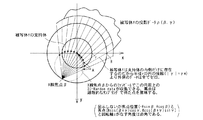
図２０及び図２１は、３次元座標系において３次元のデータ収集を概念的に説明するものである。図２０及び図２１に示すように、３次元のデータ収集は、Ｘ線焦点βからの投影データｐ（β、γ、α）（図示しない）で、Ｘ線焦点β及び面積分の対象とする平面Ｑとを含む平面（図２０中の例えば平面検出器上では直線Ｌ）に沿って積分した値を処理して、３次元ラドン空間では点Ａ（図２１）の３次元ラドンデータ（ζ、φ、ｓ）を収集することに相当する。ここで、βは投影角度（Ｘ線焦点の位置）、γはレイ角、αはコーン角度（ｘｙ平面とレイとが成す角度）をそれぞれ示す。
【００７５】
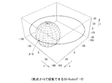
従って、図２２に示すように、Ｘ線焦点βの位置から照射されるコーンビームの全てのレイによって、Ｘ線焦点βと座標系の座標中心Ｏ（ｘ＝０、ｙ＝０、ｚ＝０）とを直径とする球面上の３次元ラドンデータが収集される。この際、前述した２次元の場合と同様に、検出器の素子が離散的で広がり（ファン角度）が限定されている場合には、上記球面上のうち、ある限定された範囲のデータが収集されることになる。
【００７６】
なお、図２３に示すように、被写体の支持体が半径ｒの球体である場合、正確な３次元再構成のためには、その球体と交わるか又は接する全ての面の面積分を収集する必要がある。
【００７７】
以上の３次元データ収集の概要を元に、３次元の再構成法を説明する。
【００７８】
まず、３次元の円軌道フルスキャンＦＳの再構成法を説明する。これは、前述した２次元のＦＳ再構成法の方法論を３次元に単純に適用したもので、本来、平面検出器（検出器面上で検出素子が均等な間隔で配列され、等距離サンプリングになる）用に開発された、Feldkamp 再構成法（「L.A. Feldkam,L.C. Davis,and J.W. Kress:“Practical cone-beam algorithm,”J. Opt. Soc. Am.,1(6),pp. 612-619,1984」参照）を、円筒検出器用に拡張した手法である（「H. Kudo and T. Saito:“Three-dimensional helical-scan computed tomography using cone-beam projection,”IEICE(D-II) J74-D-II,1108-1114(1991)」参照）。以下、この場合の手法に関しては、２次元の場合の「ＦＳ」に対し、必要に応じて「Ｆｅｌｄｋａｍｐ＋ＦＳ」と略記する。
【００７９】
この３次元の円軌道フルスキャンＦＳの再構成法は、具体的には、１回転スキャンで得られた３次元ラドンデータ（投影データ）のうちの互いに冗長なデータ同士に対し均等に重み付けするものである。これを演算式で示すと、次の式（３１）〜式（３５）で表される。
【００８０】
【数５】

【００８１】
この式（３１）〜式（３５）と、前述した２次元のＦＳの演算式（式（１）〜式（５））とを比べると、式（３２）において投影角度の積分式（逆投影部）が２次元逆投影の代わりに３次元逆投影である点と、ｃｏｓαの項が加わっている点とを除くと、全て同様となる。
【００８２】
このことを概念的に説明する。最初に、円軌道上の任意のＸ線焦点βで収集された投影データｐ（β、γ、α）を、ｃｏｓγｃｏｓαと、関数ｗ（β、γ、α）とで重み付けし（ステップ１）、その重み付けされた投影データを上記式中の関数ｇ（γ）でフィルタ処理し（ステップ２）、そのフィルタ処理されたデータを上記式中のＬ^−２（β、ｘ、ｙ）で重み付けしながら、３次元コーンビーム逆投影を行う（ステップ３）。そして、同様のステップ１〜３を円軌道上の全ての焦点位置βに対し繰り返し適用することにより、被写体ｆの画像を再構成する（ステップ４）。
【００８３】
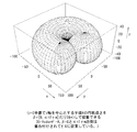
例えば、ｚ＝０の平面を回転軸ｚを中心とする円軌道上を１回だけ回転してスキャンすると、図２４に示すように、前述した図２２中の焦点及び座標中心（回転軸）を含む球体（半径ｒ）をその座標中心を中心に１回転させたときの全軌跡をカバーする領域（以下、便宜上、「りんご状領域」と呼ぶ）の３次元ラドンデータを２回ずつ収集したことになる。すなわち、ｚ＝０の平面上でみる限り、２次元のＦＳの場合と同様に、データ収集は冗長である。
【００８４】
しかし、３次元で再構成すべき被写体は、前述した図２３中の半径ｒの球体（支持体）内にあるため、この球体をカバーする領域のデータを収集する必要があるが、この点で言えば、前述の３次元のＦｅｌｄｋａｍｐ＋ＦＳでは欠落したデータがあるために不完全である。このことは、図２５に示すように、図２３と図２４とを重ね合わせた図を見ることで一目瞭然となる。すなわち、被写体の支持体を再構成するためには、Ｆｅｌｄｋａｍｐ＋ＦＳでは、本来、図２５に示す被写体を含む球体をカバーするりんご状領域のデータが必要であるにも関わらず、図２４に示すようにりんご状領域の芯部側のデータが明らかに欠落しており、これにより、必要な全ての３次元データを収集できていないことが分かる（この場合の欠落したデータを「missing data」と呼ぶことがある）。
【００８５】
なお、この３次元のＦｅｌｄｋａｍｐ＋ＦＳで得られるスライス画像の時間感度プロファイルは、前述した図１１と同様になる。
【００８６】
次に、３次元の円軌道ハーフスキャンの再構成法を説明する。ここでは、前述した３次元のＦｅｌｄｋａｍｐ＋ＦＳと同様に、２次元のＨＳの方法論を３次元に適用している。以下、この場合の手法に関しては、２次元の場合の「ＨＳ」に対し、必要に応じて「Ｆｅｌｄｋａｍｐ＋ＨＳ」と略記する。
【００８７】
この３次元のＦｅｌｄｋａｍｐ＋ＨＳでは、半回転と少しの範囲（π＋２γｍ）の円軌道上をスキャンし、ビュー方向β及びレイ方向γで連続的になるような重み関数で重み付けする。このときの重みは、コーン角αの関数ではない（全検出器列に同じ重みを乗じる）。このことを演算式で示すと、次の式（４１）〜式（４４）で表される。
【００８８】
【数６】

【００８９】
図２６は、前述した３次元Ｆｅｌｄｋａｍｐ＋ＨＳのデータ収集を概念的に説明するものである。図２６に示すように、この場合の３次元ラドンデータは、ｚ＝０の平面で回転軸ｚを中心とする半径Ｒの円軌道上をβ＝［０、π＋２γｍ］の範囲でスキャンして収集されている。
【００９０】
図２７は、図２３と図２６とを重ね合せたものである。この図２７と図２６との比較により、３次元Ｆｅｌｄｋａｍｐ＋ＨＳは、前述した３次元Ｆｅｌｄｋａｍｐ＋ＦＳの場合よりも、３次元ラドンデータの欠落領域が広がっていることが分かる。これは、２次元の再構成における方法論を単純に３次元の再構成に適用したためである。従って、３次元Ｆｅｌｄｋａｍｐ＋ＨＳでは、再構成された画像は時間分解能は高くなるものの、データ欠落領域の拡大によりアーチファクトはＦｅｌｄｋａｍｐ＋ＦＳの場合よりも強くなり、実用に耐えないといった問題があることが確認された。
【００９１】
また、前述した２次元のＭＨＳにFeldkamp 再構成法を適用したＦｅｌｄｋａｍｐ＋ＭＨＳの場合には、失うデータはＦｅｌｄｋａｍｐ＋ＨＳよりも少ないが、冗長なデータ収集を補正する重み付けが３次元ラドンデータではなく、２次元ラドンデータの収集位置に基づいているため、スキャン面以外の不正確さがＦｅｌｄｋａｍｐ＋ＦＳよりも増してしまうことはＦｅｌｄｋａｍｐ＋ＨＳと同様である。
【００９２】
次に、３次元の円軌道アンダースキャンＵＳの再構成法を説明する。これも、前述した３次元のＦｅｌｄｋａｍｐ＋ＦＳと同じく、２次元のＵＳの方法論を３次元の単純に適用したものである。以下、この場合の手法に関しては、２次元の場合の「ＵＳ」に対し、必要に応じて「Ｆｅｌｄｋａｍｐ＋ＵＳ」と略記する。
【００９３】
この３次元のＦｅｌｄｋａｍｐ＋ＵＳでは、１回転のスキャン範囲の全データを使用しているが、やはり一部のデータの重みが軽いので、Ｆｅｌｄｋａｍｐ＋ＦＳよりもデータ欠落は大きくなる。また、冗長なデータ収集に関しては、補正する重み付けが３次元ラドンデータではなく、２次元ラドンデータの収集位置に基づいているので、スキャン面以外の不正確さがＦｅｌｄｋａｍｐ＋ＦＳよりも増してしまうといった問題がある。
【００９４】
また、２次元の円軌道オーバースキャンＯＳの方法論を３次元の単純に適用した３次元の円軌道オーバースキャンＵＳの再構成法（以下、必要に応じて「Ｆｅｌｄｋａｍｐ＋ＯＳ」と略記する）の場合には、３次元ラドンデータの取得率は、３次元のＦｅｌｄｋａｍｐ＋ＦＳと同じであるが、時間分解能がＦＳと同じくＴとなり良くないといった問題がある。
【００９５】
以上の３次元再構成法のほか、「Grnatgeat 法」と呼ばれるアルゴリズムも知られている。
【００９６】
このGrnatgeat 法は、被写体が体軸方向に境界があり、検出器はみ出しがない場合（被写体が孤立物体であり、検出器が被写体全部の投影データを常に収集できる場合）、このことを専門用語で言い換えれば、「Short-object problemでdetector truncation」がない場合、焦点の軌道がＴｕｙのデータ必要条件、すなわち「被写体の支持体と交わるか又は接する全ての平面が、少なくとも一度、焦点の軌道と交わるか又は接する」の条件を満たしていれば、正確な３次元再構成が出来るものである。従って、円軌道の場合には、前述したＦｅｌｄｋａｍｐ＋ＦＳと同じく近似解となる。
【００９７】
このGrnatgeat 法による３次元再構成法のアルゴリズムは、次のステップ１〜９に示す通りである。
【００９８】
まず、焦点βで収集した投影データｐ（β、γ、α）を、ｃｏｓγｃｏｓαで重み付けし、Ｇ^（１）（β、γ、α）を得る（ステップ１）。
【００９９】
次いで、焦点βを含む平面Ｑ（ξ、φ、ｓ）に含まれるＧ^（１）（β、γ、α）を積分（平面検出器上では直線Ｌに沿って線積分）して、重み付き面積分データＧ^（２）（ξ、φ、ｓ）を得る（ステップ２）。
【０１００】
次いで、平面Ｑの近傍の平面Ｑ’（直線Ｌ’）のデータを使ってＧ^（２）（ξ、φ、ｓ）を微分して、３次元ラドンデータの１次微分データＰ^（２）（ξ、φ、ｓ）を得る（ステップ３）。
【０１０１】
次いで、上記ステップ３で得られた３次元ラドンデータの１次微分データを３次元ラドン空間に変換する（rebinning）（ステップ４）。
【０１０２】
次いで、上記ステップ１〜４を全ての焦点位置βに対して適用する（ステップ５）。
【０１０３】
次いで、３次元ラドン空間で３次元ラドンデータの冗長度を、そのラドンデータを収集した回数Ｍ（ξ、φ、ｓ）の逆数で除して補正（正規化）する（Ｍはその平面と焦点の軌道との交点の数を示す）（ステップ６）。
【０１０４】
次いで、１次微分データを半径方向に微分して２次微分データＰ^（２）（ξ、φ、ｓ）を得る（ステップ７）。
【０１０５】
次いで、２次微分データＰ^（２）（ξ、φ、ｓ）を平面Ｑ（ξ、φ、ｓ）に３次元逆投影する（ステップ８）。
【０１０６】
そして、上記ステップ６〜８の演算を、必要な全ての３次元ラドン空間のデータに繰り返し実行し、被写体ｆを再構成する（ステップ９）。
【０１０７】
また、その他の３次元再構成法として、上記のGrangeat 法の別の実装法であり、上記rebinning（ステップ４）を避けて各焦点で収集したデータを独立に扱える、「shift-variant FBP(filtered backprojection）法」と呼ばれる手法が知られている。
【０１０８】
このshift-variant FBP 法は、前述した上記Grangeat 法の条件（Ｔｕｙのデータ必要十分条件を含む）を満たしていれば、円軌道の場合にはＦｅｌｄｋａｍｐ＋ＦＳとなる（「H. Kudo and T. Saito:“Derivation and implementation of a cone-beam reconstruction algorithm for nonplanar orbits,”IEEE Trans. Med. Imag.,MI-13, pp.186-195,1994」、「M. Defrise and R. Clack:“A cone-beam reconstruction algorithm using shift-variant filtering and cone-beam backprojection,”IEEE Trans. Med. Imag., MI-13, pp.186-195,1994」等参照）。
【０１０９】
図２８（ａ）〜（ｃ）は、上記のshift-variant FBP 法を説明する概要図である。図２８（ａ）は焦点から平面検出器上へのコーンビーム投影による投影データを用いてその再投影データを得る段階（ステップ１〜２）を、図２８（ｂ）は再投影データを用いてそのコーンビーム逆投影による再構成データを得る段階（ステップ３〜９）を、図２８（ｃ）は平面検出器上でFeldkamp 法により逆投影されるデータ範囲の例を、それぞれ示す。
【０１１０】
このshift-variant FBP 法のアルゴリズムは、次のステップ１〜９に示す通りである。
【０１１１】
まず、図２８（ａ）に示すように、焦点βで収集した投影データｐ（β、ｕ、ｖ）を、ｃｏｓγｃｏｓαで重み付けし、Ｇ^（２）（β、ｕ、ｖ）を得る（ステップ１）。
【０１１２】
そして、この焦点を含む平面Ｑ（ξ、φ、ｓ）に含まれるＧ^（２）（β、ｕ、ｖ）を積分（平面検出器上では直線Ｌに沿って線積分）して、再投影データとして、重み付き面積分データＰ^（３）（ξ、φ、ｓ）を得る（ステップ２）。
【０１１３】
次いで、図２８（ｂ）に示すように、平面Ｑの近傍の平面Ｑ’（直線Ｌ’）のデータを使って、上記のＰ^（３）（θ、φ、ｓ）をフィルタ処理（微分）して、３次元ラドンデータの１次微分データＰ^（４）（ξ、φ、ｓ）を得る（ステップ３）。
【０１１４】
そして、このＰ^（４）（ξ、φ、ｓ）に重み関数Ｗを乗算することにより、データ冗長度を補正してＰ^（５）（ξ、φ、ｓ）を得る（ステップ４）。この３次元ラドンデータの１次微分Ｐ^（５）（ξ、φ、ｓ）を直線Ｌに沿って検出器面に（２次元）平行逆投影する（ステップ５）。
【０１１５】
次いで、上記ステップ２〜５の処理を検出器面上で全ての角度に適用して、Ｇ^（３）（β、ｕ、ｖ）を得る（ステップ６）。このＧ^（３）（β、ｕ、ｖ）を焦点の軌跡の接線方向（焦点の移動方向）に微分してＧ^（４）（β、ｕ、ｖ）を得る（ステップ７）。このＧ^（４）（β、ｕ、ｖ）をＬ^−２で重み付けしながら、（３次元）コーンビーム逆投影する（ステップ８）。
【０１１６】
そして、上記ステップ１〜８の処理を全焦点位置βに適用することにより、被写体ｆを再構成する（ステップ９）。
【０１１７】
上記のアルゴリズムを数式で表現すると、次の式（５１）〜式（５７）で示す通りである。
【０１１８】
【数７】

ここで、関数Ｗは、冗長度補正関数と呼ばれるもので、検出器面上の直線に対応する平面と焦点軌道との交点の数Ｍの逆数に相当する。あるいは、この関数Ｗは、交点数Ｍをスムージングしたものでもよい。上記では、平面検出器で説明してあるが、前述した通り、円筒型検出器にも適用可能であることは言うまでもない。
【０１１９】
また、上記のshift-variant FBP 法（ＦＢＰアルゴリズム）を円軌道スキャンに適用した３次元再構成法の場合には、平面と焦点軌道との交点数は常に２になるため、
【数８】

を上記式（５４）に代入すると、上記式（５１）〜（５７）を簡略化でき、Ｆｅｌｄｋａｍｐ再構成の式（３２）に帰着させることが可能である。
【０１２０】
また、上記のshift-variant FBP 法を、円と直線の組合わせからなるスキャン軌道に適用した場合には、次の条件１〜３を満たすアルゴリズムを採用することができる。
【０１２１】
１）円軌道だけと交わる平面に属するデータに関しては、平面と焦点軌道との交点数は常に２であるため、上記と同様に式（５８）を式（５４）に代入することで、式（５１）〜（５７）をFeldkamp 再構成法の式（３２）に帰着させる（条件１）。
【０１２２】
２）円軌道と直線軌道の両者と交点をもつ平面に関しては、円軌道で収集したデータに式（５８）を、また直線軌道で収集したデータに、
【数９】

を代入して使用しない（条件２）。
【０１２３】
３）円軌道と交わらずに直線軌道とのみに交点をもつ平面に属するデータに関しては、直線軌道との交点の数に応じて冗長度補正関数Ｗ_β（ｒ、θ）を与えて式（５１）〜（５７）を適用する（条件３）。
【０１２４】
以上で明らかな通り、３次元再構成における冗長度補正関数Ｗ_β（ｒ、θ）と、２次元再構成における重み関数ｗ（β、γ）は、いずれも「ｎ次元ラドンデータの冗長度を補正する」といった同じ目的を達成している。
【０１２５】
上記の冗長度補正関数Ｗ_β（ｒ、θ）の設計法に関しては、Shift-variant FBP 法の発展法が提案されている（「H. Kudo and T. Saito:“An extended completeness condition for exact cone-beam reconstruction and its application,”Conf. Rec. 1994 IEEE Med. Imag. Conf. (Norfolk, VA)(New York:IEEE)1710-14」、「H. Kudo and T. Saito: “Fast and stable cone-beam filtered backprojection method for non-planar orbits,”1998 Phys. Med. Biol. 43,pp. 747-760,1998」等参照）。これによると、冗長度補正関数Ｗ_β（ｒ、θ）は、次の目的１、２のいずれかに合せて設定される。
【０１２６】
１）専門用語で言う長大物体問題（Long-object problem）を解く。すなわち、人体の一部をスキャンする場合のように、体軸方向に長い被写体の一部を体軸歩行の幅の狭い検出器でスキャンして再構成するために、被写体はみ出しに相当する面に対応するデータに対する重みをゼロにする（目的１）。
【０１２７】
２）再構成の計算誤差を最小にする。同じ平面の誤差の少ない水平方向のramp filtering で処理できる焦点と、誤差の大きいshift-variant filtering で処理すべき焦点とに属する場合、関数Ｍを均等にせず、ramp filtering に対応するデータの重みを大きく、shift-variant filtering に対応するデータの重みを小さくする（目的２）。
【０１２８】
なお、ヘリカルスキャンの場合の正確な３次元再構成法としては、「n-PI method」と呼ばれる手法が提案されている（「R. Proksa et. al.:“The n-pi-method for helical cone-beam CT,”IEEE Trans. Med. Img., 19,848-863(2000)」参照）。本方法は、その他のヘリカルスキャンの３次元再構成法が３次元ラドンデータを冗長に収集しないのに対し、各々の３次元ラドンデータを１、３、５、７、…といったように奇数回収集するものである。従って、冗長に収集したデータは、冗長度補正関数Ｗ_β（ｒ、θ）（上記 Proksa らの文献中の式２４、すなわち
【数１０】

で示される関数が、この場合の冗長度補正関数に相当する）によって重み付けされ、補正される。
【０１２９】
従って、前述した２次元再構成法及び３次元再構成法の独自のレビューにより、正確な３次元再構成における冗長度補正関数Ｗの設定法においては、「収集時刻」という概念がなく、「被写体が動く可能性がある」という前提条件もないことが明らかになった。しかしながら、３次元再構成アルゴリズムを医用ＣＴに適用するときには、被写体である患者が動くことがあり、これを無視するとアーチファクトが生じることがある。また、時間分解能を向上したいという要求がある。
【０１３０】
（３） 本発明の３次元再構成法の原理
本発明は、前述した２次元再構成法及び３次元再構成法の独自のレビューから明確になった「被写体である患者の動きによるアーチファクトの解消および時間分解能の向上」といった要求を実現する３次元再構成法を提供する。
【０１３１】
この目的実現のため、本発明は、前述した正確な３次元再構成法において、冗長度補正関数Ｗをデータの収集時刻を元にした信頼度に基づいて設計し、その設計した冗長度補正関数Ｗを用いて３次元のラドンデータを補正するという構成を採る。
【０１３２】
ここで設計される冗長度補正関数Ｗは、データ収集が冗長であり、言い換えると同じ３次元ラドンデータを複数回収集できるスキャンの再構成法であれば、いずれの方法であってもそのまま適用できる。さらに、後述するように、信頼度の低いデータの画像への寄与率を積極的に下げた方が良い場合には、データ収集が冗長でない再構成の場合にも、上述した冗長度補正関数Ｗによる補正を適用することができる。
【０１３３】
この冗長度補正関数Ｗによる補正は、また、３次元のラドンデータのそれぞれに対して、すなわち、この各ラドンデータを演算（面積分）する対象となった平面Ｑ毎に、補正ユニット３４により実行される。
【０１３４】
ここで導入される冗長度補正関数Ｗ_β（ｒ、θ）の設計指針は、次のルール１〜３で規定される。
【０１３５】
まず、データの信頼性関数Ｔ（β）が大きく信頼できるデータ収集時刻（又は収集時刻範囲）で収集した３次元ラドンデータのそれぞれに対する重みを大きくする（ルール１）。これを数式で表現すると、次の通りである。
【０１３６】
【数１１】

【０１３７】
また、データの信頼性関数Ｔ（β）が小さく信頼できないデータ収集時刻（又は収集時刻範囲）で収集した３次元ラドンデータのそれぞれに対する重みを小さくする（ルール２）。これを数式で表現すると、次の通りである。
【０１３８】
【数１２】

【０１３９】
このルール１及び２をより具体的に説明する。
【０１４０】
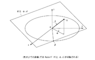
一例として、前述したように、Ｘ線管１０の焦点βが円軌道（フルスキャン）を描くように移動するスキャンの場合、この焦点βとＸ線検出器１１が提示する検出器面上の直線Ｌとを含む平面Ｑ（つまり、３次元のラドンデータのそれぞれを演算（面積分）する対象となった平面）を想定する（図２０参照）。繰返しの説明になるが、この場合、平面Ｑが円軌道の面に対して僅かでも傾いている限り、円軌道は平面Ｑに対してデータ収集時刻の異なる２箇所で交差する。この平面Ｑを面積分することにより、１つの点Ａのラドンデータが演算される（図２１参照）。したがって、２箇所で交差するということは、点Ａのラドンデータが２回収集されていることになる。
【０１４１】
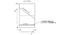
この平面Ｑと円軌道面との交差状態は、より平易には、図３３〜３４に示すように模式化できる。図中、ｔ１、ｔ２は交差する２点でのデータ収集時刻を表す。また、図３３〜３４において、（ｂ）図は、（ａ）図をある横方向Ａから見たときの模式図を示す。
【０１４２】
例えば図３３に示すデータ収集時刻ｔ１、ｔ２に対し、データ収集の冗長性を補正するため、一方のデータ収集時刻ｔ１が得たい画像の時刻であり且つこの時刻を基準に３次元ラドンデータの再構成処理を行いたいものとすると、もう一方の時刻ｔ２で収集された投影データは、一方の時刻ｔ１で収集された投影データに対しては、ｔ１〜ｔ２間に被検体が動いた可能性があるため、信頼度が低いものと推定される。この場合、時刻ｔ１で収集された投影データから演算されるラドンデータには最大の信頼度を与える一方で、時刻ｔ２で収集された投影データから演算されるラドンデータには、時刻ｔ１のそれよりも低い信頼度、すなわち、低い重みが与えられるようにする。この場合、例えば、時刻ｔ１〜ｔ２の時間差が大きくなるほど、重みが下げられるようにする。
【０１４３】
また図３４に示すデータ収集時刻ｔ１、ｔ２の場合、データ収集の冗長性を補正するため、両方の時刻ｔ１、ｔ２の中間の時刻ｔ０を得たい画像の時刻とし且つこの時刻ｔ０を基準に３次元ラドンデータの再構成処理を行いたいものとする。この場合、時刻ｔ０〜ｔ１及び時刻ｔ０〜ｔ２の時間差に応じて（例えば、それらの時間差が大きくなるにつれて）、より低い信頼度、すなわち、低い重みが与えられるようにする。
【０１４４】
また一方で、Ｘ線管１０の焦点βが円軌道（ハーフスキャン）を描くように移動するスキャンの場合、データ収集の観点からは、一部のデータ収集範囲において２箇所で交差することを除けば、焦点βの軌道は平面Ｑと１箇所でしか交差しない。この交差の様子を図３５に概念的に示す。この図３５において、（ｂ）図は、（ａ）図をある横方向Ａから見たときの模式図を示す。１箇所交差の場合、データ収集の冗長性は無い。ｔ１は交差する１点でのデータ収集時刻を表す。いま、データ収集の信頼度を考慮した補正を行うため、時刻ｔ０を得たい画像の時刻とし且つこの時刻ｔ０を基準に３次元ラドンデータの再構成処理を行いたいものとする。この場合、時刻ｔ０〜ｔ１の絶対時間差に応じて（例えば、それらの時間差が大きくなるにつれて）、より低い信頼度、すなわち、低い重みが与えられるようにする。
【０１４５】
実際には、後述するようにスキャン方法（すなわちＸ線焦点βの移動軌跡）に応じてデータ収集時刻ｔに対応した信頼度関数Ｔが決められており、この信頼度関数Ｔから冗長度補正関数Ｗによる重みが後述するように演算又は決められる。
【０１４６】
さらに、残りのルールは、同じ平面Ｑに対応する重みの積分は、０以上１以下で、データの信頼性関数の積分によって決定することである（ルール３）。これを数式で表現すると、次の通りである。
【０１４７】
【数１３】

【０１４８】
したがって、Ｘ線焦点βが円軌道を描くとすると、その円軌道に適用した場合のデータの信頼性関数Ｔ（β）は、例えば、次式（１０４）及び（１０５）で示すように収集時刻に基づいて決定される。
【０１４９】
【数１４】

【０１５０】
上記のルール１と２を具体化すると、次式（１０６）で表現される。
【０１５１】
【数１５】

【０１５２】
（データの信頼性関数の例）
本実施形態におけるデータの信頼性関数は、そのスキャン態様（例えば、円スキャン、直線スキャン、ヘリカルスキャン等）によって適宜設定されるが、その一例を図３０〜図３２に基づいて説明する。
【０１５３】
図３０は、スキャン態様が直線軌道と円１回転の軌道とから成るスキャンである場合のデータの信頼性関数Ｔ（β）又はＴ（ｔ）の例を説明するものである。
【０１５４】
この場合のスキャン軌道は、図３０中の上段グラフ（縦軸：スキャン軌道Ｚ、横軸：時間ｔ＝β）に示すように、直線方向（Ｚ軸方向、回転軸方向、又はスライス方向）の所定区間（Ｚ＝Ｚ_Ｓ〜Ｚ_Ｅ、ｔ＝ｔ_Ｓ〜ｔ_Ｅ）分、行われる直線スキャンと、これに引き続いて直線方向の一定位置（Ｚ＝Ｚ_Ｃ）で行われる円周方向の１回転（β＝０〜２π）分の円スキャンとで構成される。
【０１５５】
このスキャン軌道におけるデータの信頼性関数Ｔ（ｔ）又はＴ（β）は、例えば図３０中の中段グラフ（縦軸：Ｔ（ｔ）又はＴ（β）、横軸：ｔ又はβ）に示すように、円スキャンの中心部（β＝π）で最も信頼性が高くなるように設定される。この場合のＴ（ｔ）又はＴ（β）は、スキャンの終始点、すなわち直線スキャンの始点Ｚ_ｃ（ｔ＝ｔ_Ｓ）と、円スキャンの終点（β＝２π）で最も低く、その両者の間で、直線スキャンの始点Ｚ_ｃからその終点Ｚ_Ｅ（ｔ＝ｔ_Ｅ）を介し円スキャンの始点（ｔ＝０）を経てその中心部（β＝π）に向けて連続して増加していき、その円スキャンの中心部（β＝π）で最も高くなり、これをピークにして円スキャンの終点（β＝２π）に向けて連続して減少していくパターンとなる。
【０１５６】
これ以外の上記スキャン軌道におけるデータの信頼性関数Ｔ（ｔ）又はＴ（β）としては、図３０中の下段グラフ（縦軸：Ｔ（ｔ）又はＴ（β）、横軸：ｔ又はβ）に示すように、上記と同様に円スキャンの中心部（β＝π）で最も信頼性が高くなるように設定される一方で、直線スキャン及び円スキャンの始終点（ｔ＝ｔ_ｃ）の信頼性がほぼ同じレベルで低くなるパターンのものでもよい。
【０１５７】
図３０に示す例によれば、スキャン態様が直線と円１回転スキャンである場合により適したコーンビームＣＴによる３次元再構成アルゴリズムを構築でき、これにより、上記効果を最大限に発揮させ、被写体の動きに起因して生じるアーチファクトをより効果的に低減できる。
【０１５８】
なお、上述した図３０の例の場合、スキャンは直線軌道及び円軌道の順に１回だけなされる態様で説明したが、先に１回の円軌道のスキャンが行われ、この後に１回の直線軌道のスキャンが実行されるものであってもよい。その場合の信頼性関数は、例えば上述した図３０の中段又は下段に記した信頼性関数の時間順序を逆にすればよい。
【０１５９】
また、上述した直線軌道及び円軌道が組合されたスキャンは、複数回実行されるようにしてもよい。
【０１６０】
図３１は、スキャン態様が複数回転の連続した円軌道スキャンである場合のデータの信頼性関数Ｔ（β）又はＴ（ｔ）の設定例を説明するものである。
【０１６１】
この場合のスキャン軌道は、図３１中の最上段グラフ（縦軸：スキャン軌道Ｚ、横軸：時間ｔ＝β）に示すように、直線方向の一定位置で円周方向に連続回転させる円スキャン（β＝０〜２π〜４π〜６π）となる。このスキャン軌道におけるＴ（β）又はＴ（ｔ）は、図３１中の中央２段〜最下段の各グラフ（縦軸：Ｔ（β）又はＴ（ｔ）、横軸：ｔ＝β）に示すように、円スキャンの所定区間毎にその中央部（図中の例では、β＝０〜２π区間ではβ＝π、β＝π〜３π区間ではβ＝２π、β＝２π〜４π区間ではβ＝３π）が最も高くなるように設定される。
【０１６２】
図３１に示す例によれば、スキャン態様が複数回転の連続した円軌道スキャンである場合により適したコーンビームＣＴによる３次元再構成アルゴリズムを構築でき、これにより、上記効果を最大限に発揮させ、被写体の動きに起因して生じるアーチファクトをより効果的に低減できる。
【０１６３】
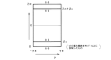
図３２は、スキャン態様がヘリカルスキャンである場合のデータの信頼性関数Ｔ（β）又はＴ（ｔ）の例を説明するものである。
【０１６４】
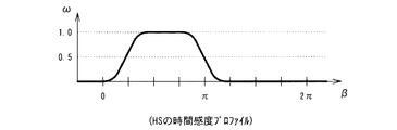
この場合のスキャン軌道は、図３２中の最上段グラフ（縦軸：スキャン軌道Ｚ、横軸：時間ｔ＝β）に示すように、直線位置を変えながら円スキャンを行うヘリカルスキャン（Ｚ＝Ｚ１〜Ｚ２〜Ｚ３〜Ｚ４、ｔ＝ｔ１〜ｔ２〜ｔ３〜ｔ４）となる。このスキャン軌道におけるＴ（β）又はＴ（ｔ）は、図３２中の中央２段〜最下段の各グラフ（縦軸：Ｔ（β）又はＴ（ｔ）、横軸：ｔ＝β）に示すように、ヘリカルスキャンの所定区間毎にその中央区間（図中の例では、上限がｔ＝ｔ３より小さい区間でｔ＝ｔ１〜ｔ２、ｔ＝ｔ１〜ｔ４の間の区間でｔ＝ｔ２〜ｔ３、上限がｔ＝ｔ４を超える区間でｔ＝ｔ３〜ｔ４）でほぼ一定値で最も高くなるパターン（略台形状パターン）に設定される。
【０１６５】
図３２に示す例によれば、スキャン態様がヘリカルスキャンである場合により適したコーンビームＣＴによる３次元再構成アルゴリズムを構築でき、これにより、上記効果を最大限に発揮させ、被写体の動きに起因して生じるアーチファクトをより効果的に低減できる。
【０１６６】
本実施形態にあっては、上述した信頼性関数Ｔを例えば式（１０６）に適用して冗長度補正関数Ｗとして演算される。この補正関数Ｗに従う重みは、補正ユニット３４又は再構成ユニット３６により求められるもので、式（１０６）などの式に基づく演算を各補正演算の度に行ってもよいし、予め補正ユニット３４の内蔵メモリ又はデータ保存ユニット３５に格納しておく記憶テーブルを参照する方法で求めてもよい。
【０１６７】
この重みを設定する手順は概略、以下のようである。まず、スキャン軌道（円軌道か、直線軌道及び円軌道の組合せ軌道かなど）及び得たい画像（再構成したい画像）の時刻が決められる。次いで、平面Ｑ毎に、スキャン軌道と平面Ｑとが交差する収集時刻（ビュー）が決められる。つまり、平面Ｑ毎に、収集されるビューが決まる。逆に言えば、各ビューで収集される平面Ｑが複数決まる。従って、各平面Ｑについて、同じ平面が収集される別のビューのデータが分かる。次いで、交差する収集時刻と上述した得たい画像の時刻との時間関係を信頼性関数に適用して、データの信頼性が決められる。次いで、この決められて信頼性を冗長度補正関数に適用して、信頼性に応じて重みが決められる。これにより、例えば、得たい画像の時刻により近い時刻で収集されたデータに、より大きな重みが設定され、一方、得たい画像の時刻から離れた時刻で収集されたデータには、相対的に小さい重みが設定される。
【０１６８】
なお、この設定は３次元再構成処理と並行して又は適宜な事前のタイミングで行っておけばよい。
【０１６９】
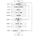
次に、上記の設計指針に基づいて求まる冗長度補正関数Ｗを用いた、実際の３次元再構成アルゴリズムによる画像再構成の処理を説明する。
【０１７０】
（Shift-variant FBP法 その１）
３次元再構成アルゴリズムとしてのShift-variant FBP 法に適用した例を説明する。この場合の処理は、図３６に示すステップＳ１０１ａ〜Ｓ１１０の順に、補正ユニット３４及び再構成ユニット３６により協働して実行される。
【０１７１】
最初に所定の収集時刻が指定され（ステップＳ１０１ａ）、検出器面上の所定角度が指定され（ステップＳ１０１ｂ）、この焦点βの位置及び検出面上の角度位置（すなわち積分対象の面に相当）で収集した投影データｐ（β、ｕ、ｖ）を、ｃｏｓγｃｏｓαで重み付けし、Ｇ^（２）（β、ｕ、ｖ）を得る（ステップＳ１０２）。
【０１７２】
次いで、焦点を含む平面Ｑ（ξ、φ、ｓ）に含まれるＧ^（２）（β、ｕ、ｖ）を積分（平面検出器上では直線Ｌに沿って線積分）して、重み付き面積分データＰ^（３）（ξ、φ、ｓ）を得る（ステップＳ１０３）。
【０１７３】
次いで、平面Ｑの近傍の平面Ｑ’（直線Ｌ’）のデータを使って、Ｐ^（３）（ξ、φ、ｓ）をフィルタ処理（微分）して、３次元ラドンデータの１次微分データＰ^（４）（ξ、φ、ｓ）を得る（ステップＳ１０４）。
【０１７４】
次いで、前述の式（１０１）〜（１０６）で求まる信頼性関数Ｔ（β）に基づいた重み関数Ｗ_β（ｒ、θ）を乗算してデータ冗長度を補正してＰ^（５）（ξ、φ、ｓ）を得る（ステップＳ１０５）。
【０１７５】
次いで、３次元ラドンデータの１次微分Ｐ^（５）（ξ、φ、ｓ）を直線Ｌに沿って検出器面に（２次元）平行逆投影する（ステップＳ１０６）。
【０１７６】
次いで、検出器面上で全ての角度に上記ステップＳ１０１ｂ〜１０６を適用してＧ^（３）（β、ｕ、ｖ）を得る（ステップＳ１０７）。
【０１７７】
次いで、焦点の軌跡の接線方向（焦点の移動方向）にＧ^（３）（β、ｕ、ｖ）を微分してＧ^（４）（β、ｕ、ｖ）を得る（ステップＳ１０８）。
【０１７８】
次いで、Ｇ^（４）（β、ｕ、ｖ）をＬ^−２で重み付けしながら、（３次元）コーンビーム逆投影する（ステップＳ１０９）。
【０１７９】
そして、上記ステップ１０１ａ〜１０９を焦点βのデータ収集範囲内の全ての位置（すなわち全収集時刻）に適用して、被写体ｆを再構成する（ステップＳ１１０）。
【０１８０】
上記のアルゴリズムを数式で表現すると、次の式（１１１）〜式（１１７）で示す通りである。
【０１８１】
【数１６】

【０１８２】
なお、本例において、信頼性関数Ｔ（β）や冗長度補正関数Ｗ_β（ｒ、θ）に負の値を持つことを許容すると外挿になり、ゼロの値の領域を広げて信頼できる区間を狭くすると、時間分解能を更に向上させることが可能となる（データ取得率を犠牲にする）。
【０１８３】
（Ｘ線焦点の直線と円とを組み合せた軌道を移動するスキャン）
その他、Ｘ線焦点βが直線と円とを組み合せた軌道を移動するスキャンの再構成法に上述した冗長度補正関数Ｗを適用した例を説明する。
【０１８４】
まず、焦点の軌道λ（β）を、次式（１２１）及び（１２２）で定義する。
【０１８５】
【数１７】

【０１８６】
このうち、次式（１２３）で示される範囲のデータを使って、被写体ｆを再構成する場合を考える。
【０１８７】
【数１８】

【０１８８】
この場合、データの信頼性関数Ｔ（β）及び冗長度補正関数Ｗ_β（ｒ、θ）は、それぞれ次式（１２４）及び（１２５）で定義される。
【０１８９】
【数１９】

【０１９０】
なお、本例の３次元再構成法は、上記のほか、Grangeat 法及びn-PI method 等の全ての３次元再構成アルゴリズムに適用可能である。また、データ収集が冗長でない再構成法であっても、「信頼の出来ないデータの重みを軽くした方が例えデータ取得率が低下しても良い結果を得ることが出来る」場合には、前述のルール１〜３の「データの信頼度に基づいて３次元ラドンデータに対する重み付けを同じ３次元ラドンデータに対する重みの総和が０〜１の間になるように決定する」という基本的な考え方は適用できる。
【０１９１】
また、本例の３次元再構成法で用いる検出器の形状は、平面検出器、円筒型検出器、球面型検出器等の任意の形状に適用できる。
【０１９２】
（shift-variant FBP法 その２）
次に、その他の３次元再構成法の例を説明する。
【０１９３】
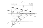
図２９は、本例のジオメトリを示すものである。図２９に示す検出器面上のジオメトリにおいて、その検出器面上の点（ｕ，ｖ）に向けて焦点βのコーンビーム頂点位置ｓ（β）（ｓはベクトル）からコーンビーム投影される投影データｇ（ｕ，ｖ，β）は、次式（１２９）及び（１３０）で与えられる円軌道に沿った演算で求められる。
【０１９４】
【数２０】

ここで、ｆ（ｒ）（ｒはベクトル）は再構成すべき被写体、Ｒは円軌道の半径、α_{ｕ，ｖ，β}は単位ベクトルをそれぞれ示す。
【０１９５】
上記のジオメトリにおいて、本適用例の３次元再構成アルゴリズムは、１）データの信頼性関数Ｔ（β）を定義し、２）３次元ラドンデータのＴ（β）に基づいて冗長度補正関数ｗ（ｓ、μ、β）を演算する、３）ｗ（ｓ、μ、β）をshift-variant FBP 法に適用するものである。以下、この内容を順次説明する。
【０１９６】
まず、データ信頼性関数Ｔ（β）に関しては、１）Ｔ（β−β_０）が│β−β_０│と共に減少する、２）∂Ｔ（β）／∂βが連続性を有するといったルールの元で、次式（１３１）及び（１３２）で定義する。
【０１９７】
【数２１】

【０１９８】
次いで、冗長度補正関数ｗ（ｓ、μ、β）に関しては、１）ｗ（ｓ、μ、β）がＴ（β）と共に増加する、２）同じ３次元ラドン面のｗ（ｓ、μ、β）における総和が１に等しくなる、３）ｗ（ｓ、μ、β）がｓ、μの座標軸において連続性を有するといったルールの元で、次式（１３３）及び（１３４）で定義する。
【０１９９】
【数２２】

【０２００】
次いで、図３７に示すステップ１２１〜１２６により、上記で求まる冗長度補正関数ｗ（ｓ、μ、β）をshift-variant FBP 法に適用して、被写体ｆを再構成する。なお、図３７に示す一連の処理は、補正ユニット３４及び再構成ユニット３６が協働して実行される。
【０２０１】
まず、所定の収集時刻及び検出器面上の位置が指定される（ステップＳ１２１，Ｓ１２２）。次に、次式（１３５）により、重み付けを行う（ステップ１２３）。
【０２０２】
【数２３】

【０２０３】
次いで、shift-variant filtering を行う（ステップ１２４）。このステップ２は、次のサブステップ２ａ〜２ｃで構成される。
【０２０４】
まず、次式（１３６）により、３次元ラドンデータを面積分で計算する（サブステップ１２４ａ）。
【０２０５】
【数２４】

【０２０６】
次いで、次式（１３７）により、冗長性補正を行う（サブステップ１２４ｂ）。これらの処理は、検出面上に設定した全ての線（すなわち面積分の対象となる全平面）について個別に繰り返される（ステップＳ１２４ｃ）。
【０２０７】
【数２５】

【０２０８】
次いで、次式（１３８）により、２次元逆投影とμ軸に沿った微分を行う（サブステップ１２４ｄ）。
【０２０９】
【数２６】

【０２１０】
そして、コーンビーム逆投影を行い、被写体ｆを再構成する（ステップ１２５）。以上の処理は、Ｘ線焦点βの必要なデータ収集範囲内の全ての位置（すなわち全収集時刻）について繰り返される（ステップＳ１２６）。
【０２１１】
上記のように構成されたＸ線ＣＴスキャナにおいて、Ｘ線管１０および２次元検出器１１がＲ−Ｒ方式で回転駆動され、マルチスキャンまたはヘリカルスキャンなどのスキャン法でＸ線投影される。この回転駆動の間、Ｘ線管１０からはＸ線が連続的に被検体Ｐに向けて曝射される。この連続Ｘ線はプリコリメータ２２によりコーン状に整形され、コーンビームとして被検体Ｐに照射される。被検体Ｐを透過したＸ線は２次元検出器１１で検出され、読み出される。これで読み出された投影データは、データ伝送部２８を通って補正ユニット３４に送られ、ここで各種の補正を受けた後、データ保存ユニット３５にビュー毎に保存される。
【０２１２】
この保存データに対し、再構成ユニット３６にて前述した３次元再構成法のいずれかのアルゴリズム（例えば、前述したステップＳ１０１ａ〜Ｓ１１０で示すアルゴリズム）に基づく画像処理が行われて被検体Ｐの再構成画像が作成され、これがメインコントローラ３０の制御の元、必要に応じてデータ保存ユニット３５に保存される一方、表示プロセッサ３７に送られ、ここでカラー化処理、アノテーションデータやスキャン情報の重畳処理などの必要な処理が行われ、ディスプレイ３８にてＤ／Ａ変換され、断層像又はボリューム像（３次元像）として表示される。
【０２１３】
以上のように、前述したファンビームのＭＨＳ（２次元の円軌道 Modified ハーフスキャン）によれば、仮想ファン角度２Γｍをπとしたときと同じ重み付けを３次元ラドンデータに対して実現しつつ、焦点回転面（ｚ＝０の平面）では２次元ファンビーム再構成におけるＭＨＳ（２Γｍ＝π）と同じ効果が得られる。すなわち、１）３次元ラドンデータのデータ取得率を信頼性に基づいた合理的な値にできる、２）時間分解能がＴ／２に向上できる、３）コーン角度の小さな領域での正確性を保てる、４）重みの連続性を保つことができるのでアーチファクトが生じない等の利点がある。
【０２１４】
従って、本実施形態によれば、コーンビームＣＴによる３次元再構成アルゴリズムを医用ＣＴに適用する際に被写体の動きに起因して生じるアーチファクトを低減すると共に、時間分解能を向上させることができる。
【０２１５】
なお、本実施形態及びその適用例では、Ｘ線ＣＴスキャナは、第３世代ＣＴに適用した例を説明してあるが、第四世代ＣＴや、高速スキャンのできる多管球ＣＴ（第３世代ＣＴでＸ線管と検出器のペアが複数あるもの）、第５世代ＣＴ（Ｘ線管を装備しないで、リング状に形成されたターゲットに対する電子ビームの衝突位置を変更してＸ線焦点を回転させるもの）等のその他のＸ線ＣＴ装置でも適用可能である。また、Ｘ線検出器についても、その形状は平面型に限定されず、円筒型など、他の形状の検出器を用いることもできる。
【０２１６】
なお、本発明は、代表的に例示した上述の実施形態及びその適用例に限定されるものではなく、当業者であれば、特許請求の範囲の記載内容に基づき、その要旨を逸脱しない範囲内で種々の態様に変形、変更することができ、それらも本発明の権利範囲に属するものである。
【０２１７】
【発明の効果】
以上説明したように、本発明によれば、コーンビームＣＴによる３次元再構成アルゴリズムを医用ＣＴに適用する際に被写体の動きに起因して生じるアーチファクトを低減できると共に、時間分解能を向上させることができる。
【図面の簡単な説明】
【図１】本発明の実施形態に係るＸ線ＣＴスキャナ（Ｘ線装置）のガントリ内のＸ線管と２次元検出器の位置関係を説明する図。
【図２】Ｘ線ＣＴスキャナの概略構成図。
【図３】Ｘ線ＣＴスキャナの電気系の概略ブロック図。
【図４】２次元のデータ収集を座標上で説明する図。
【図５】２次元ラドン空間における２次元のデータ収集を説明する図。
【図６】２次元ラドンデータを座標上で説明する図。
【図７】Ｘ線焦点からのファンビームで収集される２次元ラドンデータの集まりを座標上で説明する図。
【図８】冗長性をもつ２次元ラドンデータを説明する図。
【図９】冗長性をもつ２次元ラドンデータ収集の様子を座標上で説明する図。
【図１０】冗長性をもつ２次元ラドンデータをサイノグラム上で説明する図。
【図１１】２次元の円軌道フルスキャン（ＦＳ）の場合のスライス画像の時間感度プロファイルを示す図。
【図１２】２次元の円軌道ハーフスキャン（ＨＳ）の再構成を説明する図。
【図１３】ＨＳ再構成の場合の２次元ラドンデータをサイノグラム上で説明する図。
【図１４】ＨＳ再構成の場合のスライス画像の時間感度プロファイルを示す図。
【図１５】２次元の円軌道アンダースキャン（ＵＳ）の再構成を説明する図。
【図１６】ＵＳ再構成の場合の２次元ラドンデータをサイノグラム上で説明する図。
【図１７】ＵＳ再構成の場合のスライス画像の時間感度プロファイルを示す図。
【図１８】２次元の円軌道オーバースキャン（ＯＳ）の再構成を説明する図。
【図１９】ＯＳ再構成の場合の２次元ラドンデータをサイノグラム上で説明する図。
【図２０】３次元のデータ収集を座標上で説明する図。
【図２１】３次元ラドン空間における３次元のデータ収集を説明する図。
【図２２】ある焦点からのコーンビームで収集される３次元ラドンデータを説明する図。
【図２３】被写体を再構成するのに必要な３次元ラドンデータを説明する図。
【図２４】３次元の円軌道スキャンで収集される３次元ラドンデータを説明する図。
【図２５】図２３と図２４とを重ね合わせた図。
【図２６】３次元の円軌道ハーフスキャン（β＝［０〜π＋２γｍ］）で収集される３次元ラドンデータを説明する図。
【図２７】図２３と図２６とを重ね合わせた図。
【図２８】 shift-variant FBP 法を説明する図。
【図２９】その他の３次元再構成法の例におけるジオメトリを説明する図。
【図３０】直線と円１回転スキャンの場合のデータの信頼性関数の例を説明する図。
【図３１】複数回転の連続した円軌道スキャンの場合のデータの信頼性関数の例を説明する図。
【図３２】ヘリカルスキャンの場合のデータの信頼性関数の例を説明する図。
【図３３】データ収集の冗長性を説明する説明図。
【図３４】データ収集の冗長性を説明する別の説明図。
【図３５】冗長性の無いデータ収集を説明する説明図。
【図３６】本発明を実施した３次元再構成アルゴリズムの一例を説明する概略フローチャート。
【図３７】本発明を実施した３次元再構成アルゴリズムの別の例を説明する概略フローチャート。
【符号の説明】
１ ガントリ
２ 寝台
３ 制御キャビネット
４ 電源装置
１０ Ｘ線管
１１ ２次元検出器
２４ ＤＡＳ
３０ メインコントローラ
３１〜３３ コントローラ
３６ 再構成ユニット
３８ ディスプレイ[0001]
BACKGROUND OF THE INVENTION
The present invention relates to an X-ray CT apparatus that performs scanning using cone-beam X-rays. In particular, two-dimensional projection data of transmitted X-rays are collected by a two-dimensional detector, and three-dimensional data is obtained from the two-dimensional projection data. The present invention relates to an X-ray CT apparatus called a cone beam CT apparatus that performs reconstruction and obtains a CT image.
[0002]
[Prior art]
An X-ray CT scanner has an X-ray tube (X-ray irradiation device) and an X-ray detector arranged so that a subject is sandwiched in a gantry, and in an example driven by the RR method, for example, an X-ray tube The X-ray detector is rotated around the subject synchronously, and the X-ray beam exposed from the X-ray tube is transmitted through the subject and incident on the X-ray detector. The X-ray detector is connected to a DAS (data acquisition device), and the DAS collects transmitted X-ray intensity data for each scan, and reconstructs the projection data, thereby reconstructing the subject. Image data (slice data or volume data) can be obtained.
[0003]
In the field of such X-ray CT scanners, in recent years, as one of attempts to generate a high-resolution three-dimensional image at high speed, so-called cone beam CT, in which scanning is performed using a cone beam, has been actively studied. Yes.
[0004]
For example, according to Japanese Patent Laid-Open No. 9-19425 (see Patent Document 1), a cone beam CT that can improve the image quality by reducing the reconstruction error caused by the deviation between the actually measured X-ray path and the calculated X-ray path. An X-ray computed tomography apparatus has been proposed.
[0005]
Also, according to Japanese Patent Laid-Open No. 2000-102532 (see Patent Document 2), the scan time is exceptionally maintained while maintaining a practical circuit scale of DAS when scanning with a cone beam using continuous X-rays. There has been proposed an X-ray CT scanner as a cone beam CT that can reliably collect high-resolution projection data with few effective paths due to a shift in projection data collection timing without lengthening the projection data.
[0006]
[Patent Document 1]
Japanese Patent Laid-Open No. 9-19425
[0007]
[Patent Document 2]
JP 2000-102532 A
[0008]
[Problems to be solved by the invention]
However, if the cone beam CT proposed in the above-mentioned conventional example is applied to an actual medical CT, the patient as the subject may move. Therefore, the projection is performed with a general-purpose three-dimensional reconstruction algorithm while ignoring this. When attempting to reconstruct an image from data three-dimensionally, there are problems such as artifacts and poor time resolution.
[0009]
  The present invention has been made against the background of such a conventional situation, and even when the three-dimensional reconstruction algorithm of cone beam CT is applied to medical CT, it is possible to reduce artifacts caused by the movement of an object and to reduce time. Resolution can also be improvedX-ray CT systemThe purpose is to provide.
[0010]
[Means for Solving the Problems]
  In order to achieve the above object, according to the X-ray CT apparatus of the present invention, an X-ray source that emits cone-beam X-rays, and an X-ray that is emitted from the X-ray source and transmitted through the subject. A two-dimensional X-ray detector that detects projections and outputs projection data corresponding to the X-ray dose, and at least a predetermined scanning range under a desired scanning method involving movement of the X-ray source on a fixed trajectory A scanning unit that scans a subject with X-rays emitted from the X-ray source and causes the X-ray detector to collect the projection data associated with the scanning, and 3 from the projection data collected by the scanning unit Radon data generating means for generating three-dimensional radon data of a three-dimensional distribution, and the radon data generating meansCorresponding to each of the target areas for the area for obtaining each of the three-dimensional radon data,Weighting means for weighting the three-dimensional radon data with a weight function that exhibits a non-constant weight with respect to the projection data collection time, and reconstructing the three-dimensional radon data weighted by the weighting means with a desired three-dimensional reconstruction algorithm And reconstruction means to obtain images,The basic feature is that
[0012]
For example, the weighting unit exhibits the maximum weight at the data collection time representative of the time of the image reconstructed by the reconstruction unit as the weight function, and the small weight at the data collection time far from the data collection time. Is a means for weighting the three-dimensional radon data corresponding to the projection data collected in the scan range by using a weighting function representing
[0013]
Further, for example, the weighting unit exhibits a data collection time representing the time of the image reconstructed by the reconstruction unit and a maximum weight at a time close to the data collection time as the weight function, and these data collection times The weighting function that exhibits a small weight at a data collection time away from the image data may be used as means for weighting the three-dimensional radon data corresponding to the projection data collected in the scan range.
[0014]
Further, for example, the weighting unit exhibits a maximum weight at a data collection time representing the time of the image reconstructed by the reconstruction unit as the weight function, and a weight that decreases as the distance from the data collection time increases. It is also possible to configure as means for weighting the three-dimensional radon data corresponding to the projection data collected in the scan range using a weighting function that exhibits
[0015]
Preferably, the weight function is set according to the type of the scanning method. This scan method is, for example, a circular orbit full scan in which the orbit forms a circular orbit of one rotation, an extended circle orbit using the projection data from a 360 degree scan range in which the orbit draws a circular orbit of one rotation. Half scan (MHS: Modified Half Scan), circular trajectory underscan in which the trajectory forms a circular trajectory of one revolution, circular trajectory scan in which the trajectory presents a circular trajectory of two or more revolutions, the trajectory is a linear trajectory and a circular trajectory Or a scanning method based on a helical scan in which a trajectory in which the trajectory forms a helical trajectory.
[0018]
Specific configurations and features according to other aspects of the present invention will be made clear by embodiments of the invention described below and the accompanying drawings.
[0019]
DETAILED DESCRIPTION OF THE INVENTION
  Hereinafter, an X-ray CT apparatus according to the present invention will be described with reference to FIGS..
[0020]
The X-ray CT scanner (X-ray CT apparatus) shown in FIGS. 1 to 3 includes a gantry 1, a bed 2, a control cabinet 3, a power supply device 4, and various controllers, and is driven by, for example, the RR method. It has become. The various controllers include a high voltage controller 31, a gantry controller 33, and a bed controller 32 as shown in FIG.
[0021]
Here, as shown in FIGS. 1 and 2, the longitudinal direction of the bed 2 is defined as the column direction (or rotation axis direction or slice direction) Z, and the two directions orthogonal thereto are defined as the channel direction X and the beam exposure direction Y, respectively. Define.
[0022]
A top plate 2a is disposed on the top surface of the bed 2 so as to be slidable in the longitudinal direction (column direction Z), and the subject P is placed on the top surface of the top plate 2a. The couchtop 2a is inserted into a diagnostic opening (not shown) of the gantry 1 so as to be able to advance and retract by driving a couch driving device 2b represented by a servomotor. A driving signal is supplied from the bed controller 32 to the bed driving device 2b. The bed 2 is also provided with a position detector (not shown) such as an encoder for detecting the position of the table 2a in the longitudinal direction of the bed with an electric signal, and this detection signal is sent to the bed controller 32 as a signal for bed control. It has become.
[0023]
As shown in FIGS. 1 and 3, the gantry 1 has a substantially cylindrical rotating frame 9 therein. The above-described diagnostic opening is located inside the rotating frame 9. Further, the rotary frame 9 is provided with an X-ray tube 10 and a two-dimensional detector 11 as an X-ray detector so as to face each other with the subject P inserted in a diagnostic opening located inside thereof. . Further, at a predetermined position of the rotating frame 9, as schematically shown in FIG. 3, a high voltage generator 21, a pre-collimator 22, a scattered ray removing collimator 23 as a post-collimator, a data collecting device (DAS) 24, and A gantry driving device 25 is provided.
[0024]
Among these, the X-ray tube 10 functioning as an X-ray source has a structure of, for example, a rotating anode X-ray tube, and heats the filament by heating the filament by continuously passing a current from the high voltage generator 21 to the filament. To the target. The thermoelectrons collide with the target surface to form an effective focus, and the X-ray beam is continuously exposed from the site of the effective focus on the target surface with a spread.
[0025]
The high voltage generator 21 is supplied with a low voltage power supply from the power supply device 4 via the low voltage slip ring 26 and also receives a control signal for X-ray exposure from the high voltage controller 31 via the optical signal transmission system 27. It is done. For this reason, the high voltage generator 21 generates a high voltage from the supplied low voltage power source, generates a continuous tube voltage corresponding to the control signal from the high voltage, and supplies this to the X-ray tube 10. .
[0026]
The pre-collimator 22 is located between the X-ray tube 10 and the subject P, and the scattered radiation removing collimator 2 as a post-collimator is located between the subject P and the two-dimensional detector 11. The precollimator 22 forms, for example, a slit-shaped opening having a certain width in the column direction Z, for example. Thereby, the width of the total X-ray beam exposed from the X-ray tube 10 in the column direction Z is limited, for example, a cone having a total desired slice width corresponding to a plurality of detection element columns of the two-dimensional detector 11. Form a beam.
[0027]
The X-ray tube 10 and the two-dimensional detector 11 are rotatable in the gantry 1 so as to face each other around the axial center axis of rotation in the diagnostic opening by the rotation of the rotating frame 9.
[0028]
Further, the two-dimensional detector 11 can be applied to any one of a planar shape and a cylindrical shape, but in the description of this example, a planar shape is exemplified (the present invention is a cylindrical shape). It is also applicable to other detectors). The two-dimensional detector 11 is a detector in which a plurality of rows of detection elements having a plurality of detection channels are arranged in the slice direction (see FIG. 1). As an example, the detection unit of each detection element includes a scintillator that converts incident X-rays into an optical signal once, and converts the optical signal into an electrical signal, and a solid state detector of a photodiode. Each detection element is provided with a charge storage section (sample hold). For this reason, the two-dimensional detector 11 has a structure in which the charge accumulating unit is sequentially selected by the switch group of the DAS 24 to read out the charges, thereby detecting a signal (projection data) indicating the intensity of the transmitted X-rays. ing. In addition, as each detection element, you may use the sensor (II etc.) of the system which converts incident X-rays directly into an electrical signal.
[0029]
The DAS 24 has a so-called filter DAS structure in which detection signals are sequentially read out from each detection element and A / D converted (converted into voltage and sampled) by switching the switch group. In order to do this, the DAS 24 considers that the detector 11 is a two-dimensional detector, for example, column selection units, one channel selection unit, one A / D converter for N channels, And a control circuit.
[0030]
The data transmission unit 28 connects a signal path between the rotation side and the fixed side in the gantry 1, and here, as an example, an optical transmission system that performs signal transmission without contact is used. Note that a slip ring structure may be used as the data transmission unit 28. The digital projection data extracted via the data transmission unit 28 is sent to a correction unit (to be described later) of the control cabinet 3.
[0031]
Further, the gantry driving device 25 includes a motor, a gear mechanism, and the like that rotate the entire rotating side element in the gantry 1 together with the rotating frame 9 around its central axis. A drive signal is given to the gantry driving device 25 from the gantry controller 33.
[0032]
The high voltage controller 31, the couch controller 32, and the gantry controller 33 are interposed between the gantry 1 and the couch 2 and the control cabinet 3 in terms of signals, and each responds to a control signal from a main controller described later. Drive the load elements that you are responsible for.
[0033]
In addition to the main controller 30 that controls the entire system, the control cabinet 3 includes a correction unit 34, a data storage unit 35, a reconstruction unit 36, a display processor 37, a display 38, and an input connected to the main controller 30 via a bus. And a container 39.
[0034]
The correction unit 34 performs various correction processes such as offset correction and calibration correction on the digital amount of projection data sent from the DAS 24 in response to a processing command from the main controller 30. The corrected collected data is temporarily stored and stored in the data storage unit 35 in response to a write command from the main controller 30. The stored data is read from the data storage unit 35 in response to a read command at a desired timing of the main controller 30 and transferred to the reconstruction unit 36.
[0035]
The reconstruction unit 36 performs the three-dimensional reconstruction by applying the cone beam CT three-dimensional reconstruction method (described later) of the present invention when the collection data for reconstruction is transferred under the control of the main controller 30. A reconstruction process based on an algorithm is performed to generate image data of a three-dimensional region. The image data is stored in the data storage unit 35 as needed under the control of the main controller 30 and is sent to the display processor 37.
[0036]
The display processor 37 performs necessary processing such as colorization processing, annotation data and scan information superimposition processing on the image data, and supplies the image data to the display 38.
[0037]
The display 38 D / A converts the image data and displays it as a tomographic image.
[0038]
The input device 39 is used to give commands to the main controller 30 such as scan conditions (including the scan site and position, slice thickness, X-ray tube voltage and current, scan direction with respect to the subject, etc.) and image display conditions. .
[0039]
Here, the principle of the three-dimensional reconstruction method of the cone beam CT forming the skeleton of this embodiment will be described with reference to FIGS.
[0040]
Here, from the inventor's point of view, a known two-dimensional reconstruction method is reviewed, and the problems and factors in applying this method to the three-dimensional reconstruction method are clarified, and the book completed based on these. The three-dimensional reconstruction algorithm of the invention will be described in detail using its arithmetic expression. The n-dimensional image reconstruction means an n-dimensional inverse Radon transform, which corresponds to the subject used in this calculation (the subject P described above, and will be described below). The same shall apply.) Two-dimensional radon data (2D-Radon data) corresponding to projection data corresponding to the X-ray absorption coefficient in (2) is based on subject line integration, and three-dimensional radon data (3D-Radon data) is Depending on the area, they can be obtained.
[0041]
(1) Review of 2D reconstruction methods
First, a two-dimensional reconstruction method using a fan beam is reviewed from the viewpoint of the inventor. In general, in the case of two-dimensional data collection, the line integral data of all straight lines passing through or in contact with the subject of the two-dimensional distribution corresponds to the two-dimensional radon data (X-ray projection data), and the two-dimensional radon. Once the data is collected, complete reconstruction is possible. This will be described below with reference to FIGS. Here, in order to simplify the explanation, it is assumed that the X-ray detector is an arc detector in which detection elements are arranged in a uniform manner on an arc and capable of equiangular sampling, but as described above, in the present invention, The shape of the detector itself (arc or straight line) is not important.
[0042]
First, as shown in FIG. 4, when a virtual xy coordinate system with the rotation axis (rotation center) z of the rotation frame 9 (see above) in the gantry 1 as an origin is considered, a two-dimensional image of the subject f Is reconstructed so that a circle having a radius r including the subject f and centering around the rotation axis z is used as a support, and the two-dimensional radon space is discretely filled within the range of the support. You just have to get the data.
[0043]
Now, as shown in FIG. 5, the X-ray projection data p of the subject f collected by CT or the like corresponding to the two-dimensional radon data sets the X-ray absorption coefficient of the subject f to a certain ray in the fan beam. A set of values obtained by line integration along the line.
[0044]
For example, as shown in FIGS. 5 and 6, when the X-ray focal point of the X-ray tube 10 rotates on a circular orbit having a radius R around the rotation axis z, the X-ray focal point on the circular orbit is considered. Collecting the projection data p (β, γ) of the subject f along the ray from the position of β is that in the two-dimensional radon space, the intersection A obtained when the perpendicular is dropped from the rotation axis z onto the ray. This corresponds to collecting two-dimensional radon data (here, β represents a projection angle, that is, an X-ray focal point position, and γ (−γm to γm) represents a ray angle).
[0045]
Therefore, as shown in FIG. 7, when projection data p (β, γ) of the subject f along all rays of the fan beam irradiated from the position of the X-ray focal point β is collected, the X-ray focal point β and the rotation axis Two-dimensional radon data can be collected on a circle whose diameter is z (see solid and dotted lines in FIG. 7). In this case, when the detector elements are discretely arranged and their spread (fan angle) is limited, two-dimensional radon data within the range indicated by the solid line in FIG. 7 is collected.
[0046]
Therefore, as shown in FIGS. 8 and 9, when the X-ray focal point β is scanned by rotating once along the circular orbit of radius R around the rotation axis z on the plane of z = 0, the same point A is obtained. Since the two-dimensional radon data is collected twice, it can be seen that the data collection of this scan is executed with redundancy.
[0047]
FIG. 10 illustrates the above-described data collection using a sinogram in which the horizontal axis represents the ray angle γ (−γm to γm) and the vertical axis represents the projection angle β (0 to 2π) that is the position of the X-ray focal point. To do. In this case, for example, the two-dimensional radon data obtained when β = β shown by the solid line in the figure and the two-dimensional radon data obtained when β = π + 2γ shown by the dotted line in the figure have the same value. .
[0048]
Next, an algorithm for reconstructing an image of the subject f from two-dimensional radon data (projection data) obtained by scanning on a two-dimensional circular orbit as described above will be described.
[0049]
First, a reconstruction method of a two-dimensional circular orbit full scan (hereinafter abbreviated as “FS (Full Scan)” as necessary) will be described. In this case, redundant data among the two-dimensional radon data obtained by one rotation scan are equally weighted. This is expressed by the following equations (1) to (5).
[0050]
[Expression 1]

Here, Expression (1) is a weighting expression, and w (β, γ) is a function used for weighting. Expressions (2) to (5) are fan beam reconstruction expressions in equiangular data collection, f (x, y) is data of the subject f to be reconstructed, and g (γ) is a filter process. Function to be used, h (t) is a function used in the calculation of the function g (γ), L²(Β, x, y) indicate functions used in back projection.
[0051]
Of the above, Expression (1) is a weighting expression. This reconstruction method is a two-dimensional inverse radon transform and accurately reconstructs a cross-sectional image of the subject f.
[0052]
The above will be described conceptually. First, the projection data p (β, γ) collected at an arbitrary X-ray focal point β on the circular orbit is weighted with cos γ and the function w (β, γ) in the above equation (step 1). The weighted projection data is filtered with the function g (γ) in the above equation (step 2), and the filtered data is converted to L in the above equation.^-2Fan beam back projection is performed while weighting with (β, x, y) (step 3). The image of the subject f is reconstructed by repeatedly applying the same steps 1 to 3 to all the focal positions β on the circular orbit (step 4).
[0053]
In this reconstruction method, 1) the subject f is stationary or the motion is negligibly small, 2) the CT scanner is mechanically sufficiently stable, and the geometric error of the acquisition position can be ignored. 3) The influence of scattered radiation in the subject f can be ignored. 4) The influence of the X-ray focal point β and the size of the detection element being finite (replacement of each other) can be ignored. Is assumed.
[0054]
Therefore, according to this reconstruction method, the error due to noise can be minimized by weighting redundant data equally as in equation (1). This is because two opposing rays (see FIGS. 8 and 9) collected at different focal positions β give the same line integral value except for photon noise under the above assumptions.
[0055]
FIG. 11 illustrates a time sensitivity profile in the slice image of the subject f obtained by the above circular orbit full scan FS. The horizontal axis indicates the focal position β corresponding to time, and the vertical axis indicates the weighting function w. . In FIG. 11, the time resolution (corresponding to the half width of the profile) is the same as the time T when the X-ray focal point β rotates once.
[0056]
Next, a reconstruction method of a two-dimensional circular orbit half scan (hereinafter abbreviated as “HS (Half Scan)” as necessary) will be described. In the case of the circular orbit full scan FS that performs one rotation scan as described above, the circular orbit half scan HS collects redundantly the two-dimensional radon data, and therefore minimizes the redundancy of such data collection. In order to achieve this, scanning is performed within a half rotation and a small range (π + 2γm).
[0057]
In this circular orbit half-scan HS reconstruction method, as a function w (β, γ) used for weighting, “weight that is continuous in the view direction β and the ray direction γ” is applied to partially redundant data. Function "is used. This is expressed by the following equations (11) to (14).
[0058]
[Expression 2]

Here, the range of the focal position β in the equation (14) for obtaining f (x, y) is changed from [0, 2π] in the case of the above equation (2) to [0, π + 2γm]. In this case, in the range of β∈ [π + 2γm, 2π], x²(Β, γ) = w [x²As (β, γ)] = 0, the expression (2) may be applied as it is instead of the expression (13).
[0059]
FIG. 13 conceptually illustrates the above-described half-scan HS reconstruction method. FIG. 14 shows the sinogram, and FIG. 15 shows the time sensitivity profile at the center of the slice image obtained in this way.
[0060]
In FIG. 13, a circular graph shown outside the circular orbit indicates the weight for the central ray (γ = 0) at each X-ray focal position (projection angle). For example, at the X-ray focal point β = 0, all rays are collected again by the opposing data, so the weight is set to zero, and most of the rays are collected twice at the X-ray focal point moved from there. Since only a part of rays are collected only once at the X-ray focal point, the weight is set to 1 for rays collected only once, and the above equation (11) for rays collected twice. ) And the rule of “weight function that is continuous in view direction β and ray direction γ”, the weight is determined so as to change smoothly.
[0061]
In this scan and its reconstruction method, since the projection angle range for image reconstruction, that is, the data acquisition time is about half that of a single rotation scan, the time sensitivity at the center of the slice image shown in FIG. A profile is obtained and its time resolution is T / 2, which is very good. This coincides with the results shown in the weight graph in FIG. 12 and the sinogram in FIG. However, at the cost of improving the time resolution in this way, the number of projections (number of data, that is, the number of photons) required for image reconstruction is reduced to about half of the above circular orbit full scan FS. Will increase to about 1.4 times.
[0062]
In addition, regarding the above-described “weight function that is continuous in the view direction β and the ray direction γ”, the reconstruction shown by the above formulas (2) and (14) will be supplemented with the importance of continuity. In the calculation, a convolution operation is performed to emphasize the high frequency region in the ray direction. If the weighted data is discontinuous in the ray direction, this is emphasized more than necessary, and the final image (re-created) is reproduced. Will remain as an artifact in the constructed image). Therefore, the weight function needs to be continuous in the ray direction so as to avoid other than the discontinuous distribution such as the X-ray absorption coefficient inherent to the subject f.
[0063]
In addition, the concept of the above-described two-dimensional circular orbit half scan HS is expanded, a virtual fan angle 2Γm is introduced instead of 2γm, and a projection angle used for reconstruction is π + 2γm to 2π, so-called two-dimensional circle. Orbit Modified Half Scan (hereinafter abbreviated as “MHS (Modified Half Scan)” if necessary) (“MD Silver:“ A method for including redundant data in computed tomography, ”Med. Phys. 27, pp .773-774, 2000 "), the time resolution is T / 2.
[0064]
Next, the case of reconstruction of a two-dimensional circular orbit underscan (hereinafter abbreviated as “US (Under Scan)” if necessary) will be described.
[0065]
Here, the data obtained at the X-ray focal point at the start of acquisition (β = 0, t = 0) and the end of acquisition (β = 2π, t = T) in the FS described above is a two-dimensional radon space. However, if the subject moves during one rotation scan, it is one of the conditions assumed in the reconstruction method described above, that is, “subject f is stationary or motion can be ignored. Since “not so small” is not satisfied, the value varies greatly due to the movement of the subject f. As a result, when the above-described full-scan FS reconstruction method is used, the data becomes inconsistent, and an artifact spreading in a fan shape from the focal position of β = 0 is generated.
[0066]
Therefore, in the reconstruction of the two-dimensional circular orbit underscan US, weighting is performed in combination with the above-described FS reconstruction formula (2) in order to suppress the artifacts caused by the movement of the subject as described above. The following equations (21) and (22) are employed as the equations.
[0067]
[Equation 3]

[0068]
FIG. 15 conceptually illustrates the above-described circular orbit underscan HS reconstruction method. FIG. 16 shows the sinogram, and FIG. 17 shows the time sensitivity profile at the center of the slice image obtained in this way.
[0069]
In FIG. 15, the circular graph shown outside the circular orbit indicates the weight for the central ray (γ = 0) at each X-ray focal position (projection angle). As shown in FIGS. 15 to 17, in the circular orbit underscan HS, in order to eliminate the inconsistency of the data in the FS described above, the weighting on the data with low reliability (near β = 0, 2π) is lightened (the weight is reduced). The weights are determined so as to be as uniform as possible by collecting necessary two-dimensional Radon space data while maintaining the continuity of the weights.
[0070]
Next, the case of reconstruction of a two-dimensional circular orbit overscan (hereinafter abbreviated as “OS (Over Scan)” if necessary) will be described. This is the same purpose as in the case of the underscan described above, after scanning one extra rotation and weighting the two projection data before and after one rotation collected at the same projection angle (focal position). A reconstruction method similar to the above-described FS is used. The weighting formula in this case is as follows.
[0071]
[Expression 4]

[0072]
FIG. 18 conceptually illustrates the above-described circular orbit overscan OS reconstruction method. FIG. 19 shows the sinograms. In FIG. 19, a circular graph shown outside the circular orbit shows the weight for the central ray (γ = 0) at each X-ray focal point position (projection angle). As shown in FIGS. 18 and 19, the time resolution in this case is T.
[0073]
(2) Review of 3D reconstruction method and its problems
Next, from the viewpoint of the present inventor, the known three-dimensional reconstruction method is reviewed based on the review result of the above-described two-dimensional reconstruction method, and the problem is clarified. Here, as a two-dimensional detector, a cylindrical detector (detection elements are uniformly arranged on the cylindrical surface, and equiangular sampling in the ray direction and equidistant sampling in the z-axis direction in the xy plane) Of the detectors (detection elements are arranged at equal intervals on the detector surface and sampled equidistantly), the one that is convenient for each algorithm is assumed.
[0074]
20 and 21 conceptually explain three-dimensional data collection in a three-dimensional coordinate system. As shown in FIGS. 20 and 21, three-dimensional data collection is performed with projection data p (β, γ, α) (not shown) from the X-ray focal point β, and targets for the X-ray focal point β and area. A value integrated along a plane including the plane Q (for example, a straight line L on the flat detector in FIG. 20) is processed, and in the three-dimensional radon space, the three-dimensional radon data (ζ, This corresponds to collecting φ, s). Here, β represents a projection angle (X-ray focal point position), γ represents a ray angle, and α represents a cone angle (an angle formed by an xy plane and a ray).
[0075]
Accordingly, as shown in FIG. 22, the X-ray focal point β and the coordinate center O of the coordinate system (x = 0, y = 0, z = 0) are obtained by all rays of the cone beam irradiated from the position of the X-ray focal point β. ) And 3D radon data on a spherical surface with a diameter of. At this time, as in the case of the above-described two-dimensional case, when the detector elements are discrete and spread (fan angle) is limited, data on a limited range on the spherical surface is collected. Will be.
[0076]
As shown in FIG. 23, when the support of the subject is a sphere with a radius r, it is necessary to collect the area of all surfaces that intersect or touch the sphere for accurate three-dimensional reconstruction. There is.
[0077]
Based on the outline of the above three-dimensional data collection, a three-dimensional reconstruction method will be described.
[0078]
First, a reconstruction method of a three-dimensional circular orbit full scan FS will be described. This is a simple application of the two-dimensional FS reconstruction method methodology described above to three dimensions. Originally, a flat detector (detection elements are arranged at equal intervals on the detector surface and used for equidistant sampling. Feldkamp reconstruction method ("LA Feldkam, LC Davis, and JW Kress:" Practical cone-beam algorithm, "J. Opt. Soc. Am., 1 (6), pp. 612- 619, 1984) is an extended method for cylindrical detectors (“H. Kudo and T. Saito:“ Three-dimensional helical-scan computed tomography using cone-beam projection, ”IEICE (D-II) J74 -D-II, 1108-1114 (1991). Hereinafter, regarding the method in this case, “Feldkamp + FS” is abbreviated as necessary to “FS” in the two-dimensional case.
[0079]
Specifically, the reconstruction method of the three-dimensional circular orbit full scan FS weights the redundant data equally among the three-dimensional radon data (projection data) obtained by one rotation scan. It is. This is expressed by the following equations (31) to (35).
[0080]
[Equation 5]

[0081]
Comparing these formulas (31) to (35) with the above-described two-dimensional FS calculation formulas (formulas (1) to (5)), the integral formula of the projection angle (back projection) in formula (32) Except for the point that the part) is a three-dimensional backprojection instead of the two-dimensional backprojection and the point where the cosα term is added, all are the same.
[0082]
This will be explained conceptually. First, projection data p (β, γ, α) collected at an arbitrary X-ray focal point β on the circular orbit is weighted with cos γ cos α and a function w (β, γ, α) (step 1). The weighted projection data is filtered with the function g (γ) in the above equation (step 2), and the filtered data is converted to L in the above equation.^-2Three-dimensional cone beam backprojection is performed while weighting with (β, x, y) (step 3). The image of the subject f is reconstructed by repeatedly applying the same steps 1 to 3 to all the focal positions β on the circular orbit (step 4).
[0083]
For example, when a plane with z = 0 is rotated and scanned once on a circular orbit centered on the rotation axis z, as shown in FIG. 24, the focal point and the coordinate center (rotation axis) in FIG. Collecting three-dimensional radon data twice each for a region that covers the entire trajectory when the sphere (radius r) is rotated about its coordinate center (hereinafter referred to as “apple-shaped region”). become. That is, as long as it is seen on the plane where z = 0, data collection is redundant as in the case of the two-dimensional FS.
[0084]
However, since the object to be reconstructed in three dimensions is in the sphere (support) having the radius r in FIG. 23 described above, it is necessary to collect data of the area covering the sphere. In other words, the aforementioned three-dimensional Feldkamp + FS is incomplete because of missing data. As shown in FIG. 25, this becomes clear at a glance by looking at a diagram in which FIGS. 23 and 24 are overlapped. That is, in order to reconstruct the support of the subject, as shown in FIG. 24, although Feldkamp + FS originally needs the data of the apple-shaped region covering the sphere including the subject shown in FIG. It can be seen that the data on the core side of the apple-shaped area is clearly missing, and thus all necessary 3D data has not been collected (this missing data is called "missing data") There is).
[0085]
Note that the time sensitivity profile of the slice image obtained by this three-dimensional Feldkamp + FS is the same as that in FIG. 11 described above.
[0086]
Next, a reconstruction method of a three-dimensional circular orbit half scan will be described. Here, the two-dimensional HS methodology is applied to the third dimension, as in the above-described three-dimensional Feldkamp + FS. Hereinafter, regarding the method in this case, “Feldkamp + HS” is abbreviated as necessary to “HS” in the two-dimensional case.
[0087]
In this three-dimensional Feldkamp + HS, a half orbit and a small range (π + 2γm) are scanned on a circular orbit and weighted with a weighting function that is continuous in the view direction β and the ray direction γ. The weight at this time is not a function of the cone angle α (multiply all detector rows by the same weight). This can be expressed by the following equations (41) to (44).
[0088]
[Formula 6]

[0089]
FIG. 26 conceptually illustrates the above-described three-dimensional Feldkamp + HS data collection. As shown in FIG. 26, the three-dimensional radon data in this case is collected by scanning a circular orbit with a radius R centered on the rotation axis z in the plane of z = 0 within a range of β = [0, π + 2γm]. Has been.
[0090]
FIG. 27 is a superposition of FIG. 23 and FIG. Comparison between FIG. 27 and FIG. 26 indicates that the three-dimensional Feldkamp + HS has a larger three-dimensional radon data missing region than the above-described three-dimensional Feldkamp + FS. This is because the methodology in the two-dimensional reconstruction is simply applied to the three-dimensional reconstruction. Therefore, in the three-dimensional Feldkamp + HS, although the reconstructed image has high time resolution, it is confirmed that the artifact becomes stronger than that in the case of Feldkamp + FS due to the expansion of the data missing region, and there is a problem that it is not practical.
[0091]
Further, in the case of Feldkamp + MHS in which the Feldkamp reconstruction method is applied to the above-described two-dimensional MHS, the lost data is less than Feldkamp + HS, but the weight for correcting redundant data collection is not three-dimensional radon data but two-dimensional radon data. Since it is based on the data collection position, inaccuracies other than the scan plane increase more than Feldkamp + FS, as in Feldkamp + HS.
[0092]
Next, a reconstruction method of the three-dimensional circular orbit underscan US will be described. This is also a three-dimensional simple application of the two-dimensional US methodology, similar to the three-dimensional Feldkamp + FS described above. Hereinafter, regarding the method in this case, “Feldkamp + US” is abbreviated as necessary to “US” in the two-dimensional case.
[0093]
In this three-dimensional Feldkamp + US, all data in the scan range of one rotation is used. However, since the weight of a part of the data is also light, data omission becomes larger than that of Feldkamp + FS. Further, regarding redundant data collection, since the weight to be corrected is based on the collection position of the two-dimensional radon data, not the three-dimensional radon data, there is a problem that inaccuracies other than the scan plane increase more than Feldkamp + FS. is there.
[0094]
In the case of the reconstruction method of the three-dimensional circular orbit overscan US (hereinafter abbreviated as “Feldkamp + OS” as necessary) in which the two-dimensional circular orbit overscan OS methodology is simply applied in three dimensions. Although the acquisition rate of the three-dimensional radon data is the same as that of the three-dimensional Feldkamp + FS, there is a problem that the time resolution is not T, which is the same as the FS.
[0095]
In addition to the above three-dimensional reconstruction method, an algorithm called “Grnatgeat method” is also known.
[0096]
This Grnatgeat method uses this terminology when the subject has a boundary in the body axis direction and the detector does not protrude (when the subject is an isolated object and the detector can always collect projection data of the entire subject). In other words, in the absence of "detector truncation in a short-object problem", the focal trajectory is Tuy's data requirement, ie "all planes that meet or touch the subject support intersect the focal trajectory at least once. If the condition “or touch” is satisfied, an accurate three-dimensional reconstruction can be performed. Therefore, in the case of a circular orbit, the approximate solution is the same as the Feldkamp + FS described above.
[0097]
The algorithm of the three-dimensional reconstruction method based on this Grnatgeat method is as shown in the following steps 1 to 9.
[0098]
First, the projection data p (β, γ, α) collected at the focal point β is weighted by cos γ cos α, and G⁽¹⁾(Β, γ, α) is obtained (step 1).
[0099]
Next, G included in the plane Q (ξ, φ, s) including the focal point β.⁽¹⁾(Β, γ, α) is integrated (line integration along the straight line L on the flat detector), and weighted area data G⁽²⁾(Ξ, φ, s) is obtained (step 2).
[0100]
Next, using the data of the plane Q ′ (straight line L ′) in the vicinity of the plane Q, G⁽²⁾Differentiating (ξ, φ, s), the first derivative data P of the three-dimensional radon data⁽²⁾(Ξ, φ, s) is obtained (step 3).
[0101]
Next, the first differential data of the three-dimensional radon data obtained in step 3 is converted into a three-dimensional radon space (rebinning) (step 4).
[0102]
Next, the above steps 1 to 4 are applied to all the focal positions β (step 5).
[0103]
Next, the redundancy of the three-dimensional radon data is corrected (normalized) by dividing the redundancy of the three-dimensional radon data by the reciprocal number M (ξ, φ, s) of collecting the radon data in the three-dimensional radon space (M is the plane and the focal point). (The number of intersections with the trajectory) is indicated (step 6).
[0104]
Next, the first derivative data is differentiated in the radial direction to obtain second derivative data P⁽²⁾(Ξ, φ, s) is obtained (step 7).
[0105]
Next, secondary differential data P⁽²⁾(Ξ, φ, s) is three-dimensionally back-projected onto the plane Q (ξ, φ, s) (step 8).
[0106]
Then, the operations in steps 6 to 8 are repeatedly performed on all necessary three-dimensional radon space data to reconstruct the subject f (step 9).
[0107]
In addition, as another three-dimensional reconstruction method, another implementation method of the above Grangeat method, which avoids the rebinning (step 4) and can independently handle data collected at each focus, “shift-variant FBP (filtered A method called “backprojection method” is known.
[0108]
This shift-variant FBP method is Feldkamp + FS in the case of a circular orbit if the above-mentioned Grangeat method conditions (including Tuy's data necessary and sufficient conditions) are satisfied ("H. Kudo and T. Saito: “Derivation and implementation of a cone-beam reconstruction algorithm for nonplanar orbits,” IEEE Trans. Med. Imag., MI-13, pp.186-195, 1994 ”,“ M. Defrise and R. Clack: “A cone- beam reconstruction algorithm using shift-variant filtering and cone-beam backprojection, "IEEE Trans. Med. Imag., MI-13, pp.186-195, 1994").
[0109]
FIGS. 28A to 28C are schematic diagrams for explaining the shift-variant FBP method. FIG. 28A shows a step (steps 1 and 2) of obtaining reprojection data using projection data by cone beam projection from a focal point onto a flat detector, and FIG. 28B shows reprojection data. FIG. 28C shows an example of a data range backprojected by the Feldkamp method on the flat detector, respectively, at the stage of obtaining reconstruction data by the cone beam backprojection (steps 3 to 9).
[0110]
The algorithm of this shift-variant FBP method is as shown in the following steps 1 to 9.
[0111]
First, as shown in FIG. 28A, the projection data p (β, u, v) collected at the focal point β is weighted by cos γ cos α, and G⁽²⁾(Β, u, v) is obtained (step 1).
[0112]
G included in the plane Q (ξ, φ, s) including the focal point⁽²⁾(Β, u, v) is integrated (line integration along the straight line L on the plane detector), and weighted area data P as reprojection data⁽³⁾(Ξ, φ, s) is obtained (step 2).
[0113]
Next, as shown in FIG. 28 (b), the data of the plane Q ′ (straight line L ′) in the vicinity of the plane Q is used to obtain the above P⁽³⁾(Θ, φ, s) is filtered (differentiated) to obtain first-order differential data P of three-dimensional radon data⁽⁴⁾(Ξ, φ, s) is obtained (step 3).
[0114]
And this P⁽⁴⁾By multiplying (ξ, φ, s) by the weight function W, the data redundancy is corrected and P⁽⁵⁾(Ξ, φ, s) is obtained (step 4). First derivative P of this three-dimensional radon data⁽⁵⁾(Ξ, φ, s) is backprojected along the straight line L onto the detector surface (two-dimensional) (step 5).
[0115]
Next, apply the processing in steps 2 to 5 above to all angles on the detector surface, and G⁽³⁾(Β, u, v) is obtained (step 6). This G⁽³⁾Differentiating (β, u, v) in the tangential direction (focus movement direction) of the focal locus, G⁽⁴⁾(Β, u, v) is obtained (step 7). This G⁽⁴⁾(Β, u, v) to L^-2(3D) cone beam backprojection (step 8).
[0116]
Then, the object f is reconstructed by applying the processes in steps 1 to 8 to the omnifocal position β (step 9).
[0117]
The above algorithm is expressed by mathematical formulas as shown in the following formulas (51) to (57).
[0118]
[Expression 7]

Here, the function W is called a redundancy correction function and corresponds to the reciprocal of the number M of intersections between the plane corresponding to the straight line on the detector surface and the focal track. Alternatively, this function W may be a smoothed number of intersection points M. In the above description, the planar detector is described, but it goes without saying that the present invention can also be applied to a cylindrical detector as described above.
[0119]
In addition, in the case of the three-dimensional reconstruction method that applies the shift-variant FBP method (FBP algorithm) to the circular orbit scan, the number of intersections between the plane and the focal orbit is always 2.
[Equation 8]

Is substituted into the above equation (54), the above equations (51) to (57) can be simplified, and the Feldkamp reconstruction equation (32) can be reduced.
[0120]
Further, when the above-described shift-variant FBP method is applied to a scan trajectory composed of a combination of a circle and a straight line, an algorithm satisfying the following conditions 1 to 3 can be employed.
[0121]
1) For data belonging to a plane that intersects with only a circular orbit, the number of intersections between the plane and the focal orbit is always 2. Therefore, by substituting Expression (58) into Expression (54) as described above, Expression (54) 51) to (57) are reduced to Equation (32) of the Feldkamp reconstruction method (condition 1).
[0122]
2) For a plane that intersects with both a circular orbit and a straight orbit, the equation (58) is added to the data collected on the circular orbit and the data collected on the straight orbit is
[Equation 9]

Is not used by substituting (Condition 2).
[0123]
3) For data belonging to a plane having an intersection only with a straight orbit without intersecting with a circular orbit, the redundancy correction function W depends on the number of intersections with the straight orbit._βEquations (51) to (57) are applied by giving (r, θ) (condition 3).
[0124]
As apparent from the above, the redundancy correction function W in the three-dimensional reconstruction_β(R, θ) and the weight function w (β, γ) in the two-dimensional reconstruction both achieve the same purpose of “correcting the redundancy of n-dimensional radon data”.
[0125]
Redundancy correction function W_βRegarding the design method of (r, θ), a development method of Shift-variant FBP method has been proposed (“H. Kudo and T. Saito:“ An extended completeness condition for exact cone-beam reconstruction and its application, ” Conf. Rec. 1994 IEEE Med. Imag. Conf. (Norfolk, VA) (New York: IEEE) 1710-14, “H. Kudo and T. Saito:“ Fast and stable cone-beam filtered backprojection method for non- planar orbits, "1998 Phys. Med. Biol. 43, pp. 747-760, 1998"). According to this, the redundancy correction function W_β(R, θ) is set in accordance with either of the following purposes 1 and 2.
[0126]
1) Solve the long-object problem in technical terms. That is, in order to scan and reconstruct a part of a subject that is long in the body axis direction with a detector having a narrow body axis walking width, as in the case of scanning a part of the human body, the surface corresponding to the protrusion of the subject The weight for the corresponding data is set to zero (Purpose 1).
[0127]
2) Minimize reconstruction error. If the focus belongs to the same plane with low error horizontal ramp filtering and the focus to be processed with large error shift-variant filtering, the function M is not equalized, and the data weight corresponding to ramp filtering is Increase the data weight corresponding to the shift-variant filtering (object 2).
[0128]
As an accurate three-dimensional reconstruction method in the case of helical scanning, a method called “n-PI method” has been proposed (“R. Proksa et. Al .:“ The n-pi-method for helical cone-beam CT, "IEEE Trans. Med. Img., 19,848-863 (2000)"). This method does not collect 3D radon data redundantly, while other helical scan 3D reconstruction methods collect each 3D radon data odd times such as 1, 3, 5, 7,. To do. Therefore, the data collected redundantly is the redundancy correction function W_β(R, θ) (Equation 24 in Proksa et al.
[Expression 10]

Are weighted and corrected by the redundancy correction function in this case.
[0129]
Therefore, according to the original review of the two-dimensional reconstruction method and the three-dimensional reconstruction method described above, there is no concept of “collection time” in the method of setting the redundancy correction function W in the accurate three-dimensional reconstruction, It has become clear that there is no precondition that "There is a possibility of movement". However, when the three-dimensional reconstruction algorithm is applied to medical CT, the subject patient may move, and if this is ignored, artifacts may occur. There is also a demand to improve time resolution.
[0130]
(3) Principle of the three-dimensional reconstruction method of the present invention
The present invention realizes the requirement of “resolving artifacts due to the movement of a patient as a subject and improving temporal resolution” which has been clarified from the original review of the above-described two-dimensional reconstruction method and three-dimensional reconstruction method. A reconstruction method is provided.
[0131]
In order to achieve this object, the present invention designs the redundancy correction function W based on the reliability based on the data collection time in the above-described accurate three-dimensional reconstruction method, and the designed redundancy correction function. A configuration is adopted in which three-dimensional radon data is corrected using W.
[0132]
The redundancy correction function W designed here is redundant in data collection, in other words, any scan reconstruction method that can collect the same three-dimensional radon data multiple times can be applied as it is. . Further, as will be described later, when it is better to actively reduce the contribution rate of data with low reliability to the image, the redundancy correction function W described above is used even in the case of reconstruction in which data collection is not redundant. The correction by can be applied.
[0133]
The correction by the redundancy correction function W is also executed by the correction unit 34 for each of the three-dimensional radon data, that is, for each plane Q on which each radon data is calculated (for the area). Is done.
[0134]
Redundancy correction function W introduced here_βThe design guideline for (r, θ) is defined by the following rules 1 to 3.
[0135]
First, the weight for each of the three-dimensional radon data collected at the data collection time (or the collection time range) where the data reliability function T (β) is large and reliable is increased (rule 1). This can be expressed as follows:
[0136]
## EQU11 ##

[0137]
Further, the weight for each of the three-dimensional radon data collected at the data collection time (or the collection time range) where the data reliability function T (β) is small and unreliable is reduced (rule 2). This can be expressed as follows:
[0138]
[Expression 12]

[0139]
Rules 1 and 2 will be described more specifically.
[0140]
As an example, as described above, in the case of a scan in which the focal point β of the X-ray tube 10 moves so as to draw a circular orbit (full scan), this focal point β and a straight line on the detector surface presented by the X-ray detector 11 A plane Q including L (that is, a plane on which each of the three-dimensional radon data is calculated (area)) is assumed (see FIG. 20). In this case, as long as the plane Q is slightly inclined with respect to the plane of the circular trajectory, the circular trajectory intersects the plane Q at two points with different data collection times. By dividing the plane Q into an area, radon data of one point A is calculated (see FIG. 21). Therefore, intersecting at two places means that radon data at point A is collected twice.
[0141]
The intersecting state between the plane Q and the circular orbital plane can be simplified as shown in FIGS. In the figure, t1 and t2 represent data collection times at two intersecting points. 33 to 34, (b) shows a schematic diagram when (a) is viewed from a certain lateral direction A. FIG.
[0142]
For example, in order to correct the data collection redundancy for the data collection times t1 and t2 shown in FIG. 33, one data collection time t1 is the time of the image to be obtained, and the 3D radon data is reproduced based on this time. Assuming that the configuration processing is to be performed, the projection data collected at the other time t2 may have moved the subject between t1 and t2 with respect to the projection data collected at the other time t1. Therefore, the reliability is estimated to be low. In this case, the radon data calculated from the projection data collected at time t1 is given the maximum reliability, while the radon data calculated from the projection data collected at time t2 is given more than that at time t1. Also, a low reliability, that is, a low weight is given. In this case, for example, the weight is lowered as the time difference between the times t1 and t2 increases.
[0143]
Further, in the case of data collection times t1 and t2 shown in FIG. 34, in order to correct the redundancy of data collection, a time t0 intermediate between both times t1 and t2 is set as the time of the image to be obtained, and 3 based on this time t0. Suppose you want to reconstruct the dimensional radon data. In this case, in accordance with the time difference between the times t0 to t1 and the times t0 to t2 (for example, as the time difference increases), a lower reliability, that is, a lower weight is given.
[0144]
On the other hand, in the case of scanning in which the focal point β of the X-ray tube 10 moves so as to draw a circular orbit (half scan), from the viewpoint of data collection, except that it intersects at two points in a part of the data collection range. For example, the trajectory of the focal point β intersects the plane Q only at one place. This crossing is conceptually shown in FIG. In FIG. 35, (b) shows a schematic diagram when (a) is viewed from a certain lateral direction A. FIG. In the case of a single intersection, there is no data collection redundancy. t1 represents the data collection time at one intersecting point. Now, in order to perform correction in consideration of the reliability of data collection, it is assumed that a time t0 is set as the time of the image to be obtained, and the reconstruction process of the three-dimensional radon data is performed based on the time t0. In this case, in accordance with the absolute time difference between times t0 and t1 (for example, as the time difference increases), a lower reliability, that is, a lower weight is given.
[0145]
Actually, a reliability function T corresponding to the data acquisition time t is determined according to the scanning method (that is, the movement locus of the X-ray focal point β) as will be described later, and the redundancy correction function is determined from the reliability function T. The weight by W is calculated or determined as described later.
[0146]
Further, the remaining rule is that the integration of the weights corresponding to the same plane Q is 0 or more and 1 or less and is determined by the integration of the data reliability function (rule 3). This can be expressed as follows:
[0147]
[Formula 13]

[0148]
Therefore, if the X-ray focal point β draws a circular orbit, the reliability function T (β) of data when applied to the circular orbit is, for example, the collection time as shown by the following equations (104) and (105): To be determined.
[0149]
[Expression 14]

[0150]
More specifically, the above rules 1 and 2 are expressed by the following formula (106).
[0151]
[Expression 15]

[0152]
(Example of data reliability function)
The data reliability function in the present embodiment is appropriately set depending on the scan mode (for example, circular scan, straight line scan, helical scan, etc.), and an example thereof will be described with reference to FIGS.
[0153]
FIG. 30 illustrates an example of the data reliability function T (β) or T (t) when the scan mode is a scan composed of a linear trajectory and a circular trajectory.
[0154]
As shown in the upper graph (vertical axis: scan trajectory Z, horizontal axis: time t = β) in FIG. 30, the scan trajectory in this case is linear (Z-axis direction, rotation axis direction, or slice direction). Predetermined section (Z = Z_S~ Z_E, T = t_S~ T_E) Minutes, followed by a linear scan and a certain position in the linear direction (Z = Z_C) And a circle scan for one rotation (β = 0 to 2π) in the circumferential direction.
[0155]
The reliability function T (t) or T (β) of data in this scan trajectory is shown in, for example, the middle graph (vertical axis: T (t) or T (β), horizontal axis: t or β) in FIG. As described above, the reliability is set to be the highest at the center (β = π) of the circular scan. In this case, T (t) or T (β) is the end point of the scan, that is, the start point Z of the linear scan._c(T = t_S) And the lowest end point (β = 2π) of the circle scan, and the linear scan start point Z between them_cTo its end point Z_E(T = t_E) Through the circle scan start point (t = 0) and continuously increase toward the center (β = π), and becomes the highest at the center (β = π) of the circle scan. It becomes a pattern that continuously decreases toward the end point (β = 2π) of the circle scan with the peak at.
[0156]
As other data reliability functions T (t) or T (β) in the above scan trajectory, the lower graph in FIG. 30 (vertical axis: T (t) or T (β), horizontal axis: t or β As shown in FIG. 5B, in the same manner as described above, the highest reliability is set at the center (β = π) of the circular scan, while the start and end points of the linear scan and the circular scan (t = t_c) In which the reliability decreases at substantially the same level.
[0157]
According to the example shown in FIG. 30, it is possible to construct a three-dimensional reconstruction algorithm based on cone beam CT that is more suitable when the scan mode is a straight line and a one-round rotation scan. Artifacts caused by the movement of the can be more effectively reduced.
[0158]
In the case of the example in FIG. 30 described above, the scan is described as being performed only once in the order of the linear trajectory and the circular trajectory. However, one circular trajectory is scanned first, and then one straight line is scanned. Orbital scanning may be performed. The reliability function in that case may be reversed, for example, in the time order of the reliability functions described in the middle or lower part of FIG.
[0159]
Further, the above-described scan in which the linear track and the circular track are combined may be executed a plurality of times.
[0160]
FIG. 31 illustrates a setting example of the data reliability function T (β) or T (t) when the scan mode is a continuous circular orbit scan of a plurality of rotations.
[0161]
The scan trajectory in this case is a circular scan that is continuously rotated in the circumferential direction at a fixed position in the linear direction as shown in the uppermost graph (vertical axis: scan trajectory Z, horizontal axis: time t = β) in FIG. (Β = 0 to 2π to 4π to 6π). The T (β) or T (t) in this scan trajectory is shown in each graph (vertical axis: T (β) or T (t), horizontal axis: t = β) in the middle two stages to the lowest stage in FIG. As shown, the central portion of each predetermined period of the circular scan (in the example in the figure, β = π in the β = 0 to 2π interval, β = 2π in the β = π to 3π interval, β = 2π in the β = 2π to 4π interval, β = 3π) is set to be the highest.
[0162]
According to the example shown in FIG. 31, it is possible to construct a three-dimensional reconstruction algorithm using cone beam CT that is more suitable when the scan mode is a continuous circular orbit scan of a plurality of rotations, thereby maximizing the above effect. Artifacts caused by the movement of the subject can be reduced more effectively.
[0163]
FIG. 32 illustrates an example of the data reliability function T (β) or T (t) when the scan mode is a helical scan.
[0164]
As shown in the uppermost graph (vertical axis: scan trajectory Z, horizontal axis: time t = β) in FIG. 32, the scan trajectory in this case is a helical scan (Z = Z1) that performs a circular scan while changing the linear position. ~ Z2-Z3-Z4, t = t1-t2-t3-t4). T (β) or T (t) in this scan trajectory is shown in each graph (vertical axis: T (β) or T (t), horizontal axis: t = β) in the middle two stages to the lowest stage in FIG. As shown in the figure, for each predetermined section of the helical scan, the central section (in the example in the figure, t = t1 to t2 where the upper limit is smaller than t = t3, t = t2 to t2 between t = t1 and t4) In a section where t3 and the upper limit exceed t = t4, a pattern (substantially trapezoidal pattern) that is the highest at a substantially constant value at t = t3 to t4) is set.
[0165]
According to the example shown in FIG. 32, it is possible to construct a three-dimensional reconstruction algorithm based on cone beam CT, which is more suitable when the scan mode is a helical scan, thereby maximizing the above effect and resulting from the movement of the subject. As a result, the artifacts generated can be reduced more effectively.
[0166]
In the present embodiment, the reliability function T described above is applied to, for example, the equation (106) and is calculated as the redundancy correction function W. The weight according to the correction function W is obtained by the correction unit 34 or the reconstruction unit 36, and an operation based on an expression such as the expression (106) may be performed for each correction operation. You may obtain | require by the method of referring the memory | storage table stored in the built-in memory or the data storage unit 35. FIG.
[0167]
The procedure for setting the weight is roughly as follows. First, a scan trajectory (whether a circular trajectory or a combination of a linear trajectory and a circular trajectory) and the time of an image to be obtained (image to be reconstructed) are determined. Next, for each plane Q, an acquisition time (view) at which the scan trajectory and the plane Q intersect is determined. That is, the collected view is determined for each plane Q. In other words, a plurality of planes Q collected in each view are determined. Therefore, for each plane Q, the data of another view in which the same plane is collected is known. Next, the reliability of the data is determined by applying the time relationship between the intersecting acquisition time and the time of the desired image to be obtained to the reliability function. The determined reliability is then applied to the redundancy correction function to determine the weight according to the reliability. Thereby, for example, a larger weight is set to data collected at a time closer to the time of the image to be obtained, while relatively small is set to data collected at a time away from the time of the image to be obtained. A weight is set.
[0168]
This setting may be performed in parallel with the three-dimensional reconstruction process or at an appropriate advance timing.
[0169]
Next, an image reconstruction process using an actual three-dimensional reconstruction algorithm using the redundancy correction function W obtained based on the above design guidelines will be described.
[0170]
(Shift-variant FBP method 1)
An example applied to the Shift-variant FBP method as a three-dimensional reconstruction algorithm will be described. The processing in this case is executed in cooperation with the correction unit 34 and the reconstruction unit 36 in the order of steps S101a to S110 shown in FIG.
[0171]
First, a predetermined collection time is specified (step S101a), a predetermined angle on the detector surface is specified (step S101b), and the position of the focal point β and the angular position on the detection surface (that is, corresponding to the integration target surface). The projection data p (β, u, v) collected in step S is weighted by cos γ cos α, and G⁽²⁾(Β, u, v) is obtained (step S102).
[0172]
Next, G included in the plane Q (ξ, φ, s) including the focal point⁽²⁾(Β, u, v) is integrated (line integration along the straight line L on the plane detector), and weighted area data P⁽³⁾(Ξ, φ, s) is obtained (step S103).
[0173]
Next, using the data of the plane Q ′ (straight line L ′) in the vicinity of the plane Q, P⁽³⁾(Ξ, φ, s) is filtered (differentiated) to obtain first-order differential data P of three-dimensional radon data.⁽⁴⁾(Ξ, φ, s) is obtained (step S104).
[0174]
Next, the weighting function W based on the reliability function T (β) obtained by the above-described equations (101) to (106)._βMultiply (r, θ) to correct the data redundancy and P⁽⁵⁾(Ξ, φ, s) is obtained (step S105).
[0175]
Next, the first derivative P of the 3D radon data⁽⁵⁾(Ξ, φ, s) is (2D) parallel backprojected onto the detector surface along the straight line L (step S106).
[0176]
Next, the above steps S101b to 106 are applied to all angles on the detector surface to obtain G⁽³⁾(Β, u, v) is obtained (step S107).
[0177]
Next, G in the tangential direction (focus movement direction) of the focus locus⁽³⁾Differentiate (β, u, v) to give G⁽⁴⁾(Β, u, v) is obtained (step S108).
[0178]
Then G⁽⁴⁾(Β, u, v) to L^-2(3D) cone beam backprojection while weighting with (Step S109).
[0179]
Then, the above steps 101a to 109 are applied to all positions within the data collection range of the focus β (that is, all collection times) to reconstruct the subject f (step S110).
[0180]
The above algorithm is expressed by mathematical formulas as shown in the following formulas (111) to (117).
[0181]
[Expression 16]

[0182]
In this example, the reliability function T (β) and the redundancy correction function W_βAllowing (r, θ) to have a negative value is extrapolated, and if the range of zero values is expanded and the reliable section is narrowed, the time resolution can be further improved (data acquisition rate). Sacrificing).
[0183]
(Scan to move along a trajectory combining X-ray focal lines and circles)
In addition, an example in which the above-described redundancy correction function W is applied to a scan reconstruction method in which the X-ray focal point β moves on a trajectory combining a straight line and a circle will be described.
[0184]
First, the focal path λ (β) is defined by the following equations (121) and (122).
[0185]
[Expression 17]

[0186]
Of these, a case is considered in which the subject f is reconstructed using data in the range represented by the following equation (123).
[0187]
[Formula 18]

[0188]
In this case, the data reliability function T (β) and the redundancy correction function W_β(R, θ) is defined by the following equations (124) and (125), respectively.
[0189]
[Equation 19]

[0190]
The three-dimensional reconstruction method of this example is applicable to all three-dimensional reconstruction algorithms such as the Grangeat method and the n-PI method in addition to the above. Even if the data collection is a non-redundant reconstruction method, in the case where “the result of reducing the data acquisition rate can be obtained by reducing the weight of unreliable data,” for example, Rules 1 to 3 in which the basic idea that “the weight of the three-dimensional radon data is determined so that the sum of the weights of the same three-dimensional radon data is between 0 and 1 based on the reliability of the data” is applied. it can.
[0191]
The shape of the detector used in the three-dimensional reconstruction method of this example can be applied to any shape such as a flat detector, a cylindrical detector, a spherical detector, and the like.
[0192]
(Shift-variant FBP method 2)
Next, examples of other three-dimensional reconstruction methods will be described.
[0193]
FIG. 29 shows the geometry of this example. In the geometry on the detector surface shown in FIG. 29, the projection is cone-beam projected from the cone beam vertex position s (β) (s is a vector) of the focal point β toward the point (u, v) on the detector surface. The data g (u, v, β) is obtained by calculation along a circular orbit given by the following equations (129) and (130).
[0194]
[Expression 20]

Here, f (r) (r is a vector) is a subject to be reconstructed, R is a radius of a circular orbit, α_{u, v, β}Indicates a unit vector.
[0195]
In the above geometry, the 3D reconstruction algorithm of this application example defines 1) a data reliability function T (β), and 2) a redundancy correction function w based on T (β) of 3D radon data. (S, μ, β) is calculated. 3) w (s, μ, β) is applied to the shift-variant FBP method. Hereinafter, the contents will be sequentially described.
[0196]
First, regarding the data reliability function T (β), 1) T (β−β₀) Is │β-β₀2) It is defined by the following equations (131) and (132) under the rule that ∂T (β) / ∂β has continuity.
[0197]
[Expression 21]

[0198]
Then, for the redundancy correction function w (s, μ, β), 1) w (s, μ, β) increases with T (β), 2) w (s, μ, The sum of β) is equal to 1, and 3) w (s, μ, β) is defined by the following expressions (133) and (134) under the rule that s and μ have continuity in the coordinate axes.
[0199]
[Expression 22]

[0200]
Next, in steps 121 to 126 shown in FIG. 37, the redundancy correction function w (s, μ, β) obtained above is applied to the shift-variant FBP method to reconstruct the subject f. Note that a series of processing shown in FIG. 37 is executed in cooperation with the correction unit 34 and the reconstruction unit 36.
[0201]
First, a predetermined collection time and a position on the detector surface are designated (steps S121 and S122). Next, weighting is performed according to the following equation (135) (step 123).
[0202]
[Expression 23]

[0203]
Next, shift-variant filtering is performed (step 124). This step 2 includes the following sub-steps 2a to 2c.
[0204]
First, the three-dimensional radon data is calculated for the area by the following equation (136) (substep 124a).
[0205]
[Expression 24]

[0206]
Next, redundancy correction is performed by the following equation (137) (substep 124b). These processes are individually repeated for all the lines set on the detection surface (that is, all planes to be covered by the area) (step S124c).
[0207]
[Expression 25]

[0208]
Next, two-dimensional backprojection and differentiation along the μ axis are performed by the following equation (138) (substep 124d).
[0209]
[Equation 26]

[0210]
Then, cone beam back projection is performed to reconstruct the subject f (step 125). The above process is repeated for all positions (that is, all acquisition times) within the necessary data collection range of the X-ray focal point β (step S126).
[0211]
In the X-ray CT scanner configured as described above, the X-ray tube 10 and the two-dimensional detector 11 are rotationally driven by the RR method, and are X-ray projected by a scanning method such as multi-scan or helical scan. During this rotational drive, X-rays are continuously exposed from the X-ray tube 10 toward the subject P. The continuous X-ray is shaped into a cone shape by the pre-collimator 22 and irradiated onto the subject P as a cone beam. X-rays that have passed through the subject P are detected and read by the two-dimensional detector 11. The projection data read out in this way is sent to the correction unit 34 through the data transmission unit 28, and after being subjected to various corrections, is stored in the data storage unit 35 for each view.
[0212]
The stored data is subjected to image processing based on one of the algorithms of the three-dimensional reconstruction method described above (for example, the algorithm shown in steps S101a to S110 described above) in the reconstruction unit 36, and the object P is reconstructed. A configuration image is created, and is stored in the data storage unit 35 as necessary under the control of the main controller 30, while being sent to the display processor 37, where colorization processing, annotation data, and superimposition processing of scan information are performed. Necessary processing such as the above is performed, D / A conversion is performed on the display 38, and a tomographic image or a volume image (three-dimensional image) is displayed.
[0213]
As described above, according to the MHS (two-dimensional circular orbit modified half scan) of the fan beam described above, the same weighting as that when the virtual fan angle 2Γm is set to π is realized for the three-dimensional radon data, while focusing. The same effect as MHS (2Γm = π) in the two-dimensional fan beam reconstruction can be obtained on the rotation plane (plane where z = 0). In other words, 1) the data acquisition rate of 3D radon data can be set to a reasonable value based on reliability, 2) the time resolution can be improved to T / 2, and 3) accuracy in a small cone angle region can be maintained. 4) Since the continuity of weights can be maintained, there are advantages such as no artifacts.
[0214]
Therefore, according to the present embodiment, it is possible to reduce the artifacts caused by the movement of the subject when applying the three-dimensional reconstruction algorithm based on the cone beam CT to the medical CT, and to improve the time resolution.
[0215]
In this embodiment and its application example, the X-ray CT scanner has been described as being applied to the third generation CT. However, the fourth generation CT and a multi-tube CT (third generation CT) capable of high-speed scanning are described. CT with multiple X-ray tube and detector pairs), 5th generation CT (without the X-ray tube, changing the collision position of the electron beam to the ring-shaped target to change the X-ray focus It can be applied to other X-ray CT apparatuses such as those that rotate. Further, the shape of the X-ray detector is not limited to the planar type, and a detector having another shape such as a cylindrical type can also be used.
[0216]
It should be noted that the present invention is not limited to the above-described exemplary embodiments and application examples thereof, and those skilled in the art are within the scope of the present invention based on the description of the claims. Thus, various modifications and changes can be made to various embodiments, and these also belong to the scope of the right of the present invention.
[0217]
【The invention's effect】
As described above, according to the present invention, when a three-dimensional reconstruction algorithm based on cone beam CT is applied to medical CT, it is possible to reduce artifacts caused by the movement of the subject and improve time resolution. it can.
[Brief description of the drawings]
FIG. 1 is a view for explaining the positional relationship between an X-ray tube and a two-dimensional detector in a gantry of an X-ray CT scanner (X-ray apparatus) according to an embodiment of the present invention.
FIG. 2 is a schematic configuration diagram of an X-ray CT scanner.
FIG. 3 is a schematic block diagram of an electric system of an X-ray CT scanner.
FIG. 4 is a diagram illustrating two-dimensional data collection on coordinates.
FIG. 5 is a diagram for explaining two-dimensional data collection in a two-dimensional Radon space.
FIG. 6 is a diagram illustrating two-dimensional radon data on coordinates.
FIG. 7 is a diagram for explaining, on coordinates, a collection of two-dimensional radon data collected by a fan beam from an X-ray focal point.
FIG. 8 is a diagram illustrating two-dimensional radon data having redundancy.
FIG. 9 is a diagram for explaining the state of collecting two-dimensional radon data having redundancy on coordinates.
FIG. 10 is a diagram for explaining two-dimensional radon data having redundancy on a sinogram.
FIG. 11 is a diagram showing a time sensitivity profile of a slice image in the case of a two-dimensional circular orbit full scan (FS).
FIG. 12 is a view for explaining reconstruction of a two-dimensional circular orbit half scan (HS).
FIG. 13 is a diagram for explaining two-dimensional radon data in the case of HS reconstruction on a sinogram.
FIG. 14 is a diagram showing a time sensitivity profile of a slice image in the case of HS reconstruction.
FIG. 15 is a diagram illustrating reconstruction of a two-dimensional circular orbit underscan (US).
FIG. 16 is a view for explaining two-dimensional radon data in the case of US reconstruction on a sinogram.
FIG. 17 is a diagram showing a time sensitivity profile of a slice image in the case of US reconstruction.
FIG. 18 is a diagram illustrating reconstruction of a two-dimensional circular orbit overscan (OS).
FIG. 19 is a view for explaining two-dimensional radon data in the case of OS reconstruction on a sinogram.
FIG. 20 is a diagram illustrating three-dimensional data collection on coordinates.
FIG. 21 is a diagram illustrating three-dimensional data collection in a three-dimensional radon space.
FIG. 22 is a diagram for explaining three-dimensional radon data collected with a cone beam from a certain focal point.
FIG. 23 is a diagram for explaining three-dimensional radon data necessary for reconstructing a subject.
FIG. 24 is a diagram for explaining three-dimensional radon data collected by a three-dimensional circular orbit scan.
FIG. 25 is a diagram in which FIG. 23 and FIG. 24 are superimposed.
FIG. 26 is a view for explaining three-dimensional radon data collected by a three-dimensional circular orbit half scan (β = [0 to π + 2γm]).
FIG. 27 is a diagram in which FIG. 23 and FIG. 26 are superimposed.
FIG. 28 is a diagram for explaining the shift-variant FBP method.
FIG. 29 is a diagram illustrating geometry in another example of the three-dimensional reconstruction method.
FIG. 30 is a diagram for explaining an example of a reliability function of data in the case of a straight line and one circle scan.
FIG. 31 is a diagram for explaining an example of a data reliability function in the case of continuous circular orbit scanning of a plurality of rotations;
FIG. 32 is a diagram for explaining an example of a data reliability function in the case of a helical scan.
FIG. 33 is an explanatory diagram for explaining data collection redundancy;
FIG. 34 is another explanatory diagram for explaining data collection redundancy;
FIG. 35 is an explanatory diagram for explaining data collection without redundancy;
FIG. 36 is a schematic flowchart illustrating an example of a three-dimensional reconstruction algorithm embodying the present invention.
FIG. 37 is a schematic flowchart for explaining another example of the three-dimensional reconstruction algorithm embodying the present invention.
[Explanation of symbols]
1 Gantry
2 sleeper
3 Control cabinet
4 Power supply
10 X-ray tube
11 Two-dimensional detector
24 DAS
30 Main controller
31-33 controller
36 reconstruction units
38 display

Claims (8)

An X-ray source that emits cone-beam X-rays;
A two-dimensional X-ray detector that detects X-rays emitted from the X-ray source and transmitted through the subject and outputs projection data corresponding to the X-ray dose;
The subject is scanned with X-rays exposed from the X-ray source in a predetermined scanning range under a desired scanning method involving movement of the X-ray source on a fixed orbit, and the scanning accompanying the scanning is performed. Scanning means for causing the X-ray detector to collect projection data;
Radon data generating means for generating three-dimensional radon data of a three-dimensional distribution from the projection data collected by the scanning means;
A non-constant weight is given to the three-dimensional radon data with respect to the time of collection of the projection data , corresponding to each of the areas corresponding to the area for obtaining each of the three-dimensional radon data generated by the radon data generating means. A weighting means for performing weighting by a weight function to be presented ;
Reconstruction means for obtaining an image by reconstructing the three-dimensional radon data weighted by the weighting means with a desired three-dimensional reconstruction algorithm ;
An X-ray CT apparatus comprising:   The scanning means moves the X-ray source so as to draw a trajectory including at least “180 degrees + fan angle of the cone beam X-ray” as the scanning range around the subject as the constant trajectory. The X-ray CT apparatus according to claim 1, wherein the X-ray CT apparatus is configured to allow the X-ray CT apparatus to operate. The weighting means presents a maximum weight at a data collection time representing the time of the image reconstructed by the reconstruction means as the weight function, and a small weight at a data collection time away from the data collection time. using the weight function, X-rays CT apparatus according to claim 1, wherein the means for the weighting to the three-dimensional radon data corresponding to the projection data collected in the scan range. The weighting means presents a maximum weight at a data collection time representing the time of the image reconstructed by the reconstruction means and a time close to the data collection time as the weight function, and is away from the data collection time The X-ray CT apparatus according to claim 1 , wherein the X-ray CT apparatus is a unit that weights the three-dimensional radon data corresponding to the projection data collected in the scan range by using a weight function that exhibits a small weight at a data collection time. The weighting means presents a maximum weight at the data collection time that represents the time of the image reconstructed by the reconstruction means as the weight function, and a weight function that exhibits a weight that decreases with increasing distance from the data collection time. using, X-rays CT apparatus according to claim 1, wherein the means for the weighting to the three-dimensional radon data corresponding to the projection data collected in the scan range. The X-ray CT apparatus according to claim 1 , wherein the weighting function is set according to a type of the scanning method. The scan method includes a circular orbit full scan in which the orbit forms a circular orbit of one rotation, an extended circle orbit half scan using a projection data from a 360-degree scan range in which the orbit draws a circular orbit of one rotation. (MHS: Modified Half Scan), circular trajectory underscan in which the trajectory forms a circular trajectory of one revolution, circular trajectory scan in which the trajectory presents a circular trajectory of two revolutions or more, and the trajectory combines a linear trajectory and a circular trajectory The X-ray CT apparatus according to claim 6 , wherein the X-ray CT apparatus is a scan method based on a combined scan or a scan based on a helical scan that draws a helical trajectory. And further providing means for determining the weighting function from the reliability of the projection data determined in advance according to the collection time of the projection data for each surface, and providing weight information based on the weighting function for each surface. Item 8. The X-ray CT apparatus according to any one of Items 2 to 7 .

Images