JP2016519487A - Compilers and methods for software defined networks - Google Patents
Compilers and methods for software defined networks Download PDFInfo
- Publication number
- JP2016519487A JP2016519487A JP2016504588A JP2016504588A JP2016519487A JP 2016519487 A JP2016519487 A JP 2016519487A JP 2016504588 A JP2016504588 A JP 2016504588A JP 2016504588 A JP2016504588 A JP 2016504588A JP 2016519487 A JP2016519487 A JP 2016519487A
- Authority
- JP
- Japan
- Prior art keywords
- network
- mapping
- node
- physical
- topology
- Prior art date
- Legal status (The legal status is an assumption and is not a legal conclusion. Google has not performed a legal analysis and makes no representation as to the accuracy of the status listed.)
- Pending
Links
Images


Classifications
-
- H—ELECTRICITY
- H04—ELECTRIC COMMUNICATION TECHNIQUE
- H04L—TRANSMISSION OF DIGITAL INFORMATION, e.g. TELEGRAPHIC COMMUNICATION
- H04L41/00—Arrangements for maintenance, administration or management of data switching networks, e.g. of packet switching networks
- H04L41/12—Discovery or management of network topologies
- H04L41/122—Discovery or management of network topologies of virtualised topologies, e.g. software-defined networks [SDN] or network function virtualisation [NFV]
-
- H—ELECTRICITY
- H04—ELECTRIC COMMUNICATION TECHNIQUE
- H04L—TRANSMISSION OF DIGITAL INFORMATION, e.g. TELEGRAPHIC COMMUNICATION
- H04L41/00—Arrangements for maintenance, administration or management of data switching networks, e.g. of packet switching networks
- H04L41/14—Network analysis or design
- H04L41/145—Network analysis or design involving simulating, designing, planning or modelling of a network
-
- H—ELECTRICITY
- H04—ELECTRIC COMMUNICATION TECHNIQUE
- H04L—TRANSMISSION OF DIGITAL INFORMATION, e.g. TELEGRAPHIC COMMUNICATION
- H04L41/00—Arrangements for maintenance, administration or management of data switching networks, e.g. of packet switching networks
- H04L41/34—Signalling channels for network management communication
- H04L41/342—Signalling channels for network management communication between virtual entities, e.g. orchestrators, SDN or NFV entities
-
- H—ELECTRICITY
- H04—ELECTRIC COMMUNICATION TECHNIQUE
- H04L—TRANSMISSION OF DIGITAL INFORMATION, e.g. TELEGRAPHIC COMMUNICATION
- H04L41/00—Arrangements for maintenance, administration or management of data switching networks, e.g. of packet switching networks
- H04L41/40—Arrangements for maintenance, administration or management of data switching networks, e.g. of packet switching networks using virtualisation of network functions or resources, e.g. SDN or NFV entities
-
- H—ELECTRICITY
- H04—ELECTRIC COMMUNICATION TECHNIQUE
- H04L—TRANSMISSION OF DIGITAL INFORMATION, e.g. TELEGRAPHIC COMMUNICATION
- H04L45/00—Routing or path finding of packets in data switching networks
- H04L45/64—Routing or path finding of packets in data switching networks using an overlay routing layer
-
- H—ELECTRICITY
- H04—ELECTRIC COMMUNICATION TECHNIQUE
- H04L—TRANSMISSION OF DIGITAL INFORMATION, e.g. TELEGRAPHIC COMMUNICATION
- H04L45/00—Routing or path finding of packets in data switching networks
- H04L45/74—Address processing for routing
-
- H—ELECTRICITY
- H04—ELECTRIC COMMUNICATION TECHNIQUE
- H04L—TRANSMISSION OF DIGITAL INFORMATION, e.g. TELEGRAPHIC COMMUNICATION
- H04L67/00—Network arrangements or protocols for supporting network services or applications
- H04L67/01—Protocols
- H04L67/10—Protocols in which an application is distributed across nodes in the network
- H04L67/1097—Protocols in which an application is distributed across nodes in the network for distributed storage of data in networks, e.g. transport arrangements for network file system [NFS], storage area networks [SAN] or network attached storage [NAS]
-
- H—ELECTRICITY
- H04—ELECTRIC COMMUNICATION TECHNIQUE
- H04L—TRANSMISSION OF DIGITAL INFORMATION, e.g. TELEGRAPHIC COMMUNICATION
- H04L45/00—Routing or path finding of packets in data switching networks
- H04L45/12—Shortest path evaluation
- H04L45/123—Evaluation of link metrics
-
- H—ELECTRICITY
- H04—ELECTRIC COMMUNICATION TECHNIQUE
- H04L—TRANSMISSION OF DIGITAL INFORMATION, e.g. TELEGRAPHIC COMMUNICATION
- H04L45/00—Routing or path finding of packets in data switching networks
- H04L45/58—Association of routers
- H04L45/586—Association of routers of virtual routers
Landscapes
- Engineering & Computer Science (AREA)
- Computer Networks & Wireless Communication (AREA)
- Signal Processing (AREA)
- Data Exchanges In Wide-Area Networks (AREA)
Abstract
方法と論理的なネットワークモデルに基づいてネットワークを制御するためのコンパイラ。ネットワークは、物理ノードと仮想ノードを持っています。物理ノードは、物理的なネットワークレイアウトに従って、物理リンクによって相互接続されています。論理的なネットワークモデルは、ネットワーク内の少なくとも1つの物理的または少なくとも1つの仮想ノードを指す論理ノード名で示される論理ノードを有しています。この方法は、物理的な転送ポリシーに依存して物理ネットワークの物理パスを定義する物理的な転送ポイントオブアタッチメント関係を使用して、仮想ノードと物理ノードが相互にマッピングする方法を規定する第1のマッピング関係、および第2のマッピング論理ノードが物理ノードと仮想ノードにマップする方法を定義する関係。この方法はまた、物理ノードと仮想の間の物理的な転送ポイントオブアタッチメント関係の最初のマッピング関係に依存して物理ノードと仮想ノード間のパスに物理的にネットワーク内で変換するパスと同様に、変換する経路を含みます物理ノードと仮想ノード間及び第2のマッピング関係上のパスに依存して、論理ノード間の可能なリンク関係にノード。論理ネットワーク内の論理パスを定義するポイントオブアタッチメント関係論理転送が計算され、転送テーブルのエントリは、論理的な転送ポイントオブアタッチメント関係から物理ノードと仮想ノードのために作成されています。Compiler for controlling networks based on methods and logical network models. The network has physical nodes and virtual nodes. The physical nodes are interconnected by physical links according to the physical network layout. A logical network model has a logical node indicated by a logical node name that points to at least one physical or at least one virtual node in the network. This method uses a physical transfer point-of-attachment relationship that defines the physical path of the physical network depending on the physical transfer policy, and the first method specifies how virtual nodes and physical nodes map to each other. Mapping relationship and the relationship that defines how the second mapping logical node maps to physical and virtual nodes. This method is also similar to a path that physically translates in the network to a path between the physical node and the virtual node depending on the initial mapping relationship of the physical transfer point of attachment relationship between the physical node and the virtual. Depending on the path on the second mapping relationship between the physical node and the virtual node, including the path to convert, the node into a possible link relationship between the logical nodes. Point-of-attachment relationships that define logical paths in the logical network are calculated, and forwarding table entries are created for physical and virtual nodes from the logical transfer point-of-attachment relationships.
Description
本発明は、通信ネットワークおよびコンピューティング装置にも関します。
このようなネットワークは、パケット交換されてもよいです。
特に、本発明は、パケット転送装置、コンピュータ機器、仮想スイッチと物理的および仮想ネットワーク内の仮想マシンを構成するための方法に関する。
The invention also relates to communication networks and computing devices.
Such networks may be packet switched.
In particular, the present invention relates to packet forwarding devices, computer equipment, virtual switches and methods for configuring virtual machines in physical and virtual networks.
パケットのフィールドの最近の開発は、ネットワーク(PSN)を交換し、コンピューティングは、ソフトウェア定義ネットワーク(SDN)の概念につながりました。
適切に指示し、本発明の文脈において、我々は、高レベル仕様のネットワークを定義する機能として、ネットワークソフトウェア定義考える(例えばし、しかし、高レベルのプログラミングまたはスクリプト言語に限定されない)自動化されたプロセスを介しこの仕様に応じて、物理および仮想ネットワークやコンピューティングリソース。
このような最近の動向は、「仮想スイッチを実装し、管理するための方法および装置」WO2010115060に発見され、WO2012082988「ネットワークスイッチの設定方法」をすることができます。
最近では、標準化されたプロトコルを介してオープンインタフェースを使用して所望の転送動作をパケット転送装置に指示することが可能となりました。
このため、現在の大手プロトコルはOpenFlowをであるが、本発明は、限定されたかのOpenFlowプロトコルに結合したが、自然の中で一般的なものではなく、パケット転送装置の転送テーブル(複数可)へのプログラムによるアクセスを提供し、将来のプロトコルで動作することができます。
転送テーブル(複数可)にからパケットを転送するために所望の出力ポートを提供し、マッチングされ、着信パケットの入力ポートからの情報に対する情報が含まれています。
我々は、システム間相互接続(OSI)レイヤ2を開くために限定されるものではなく、パケット転送を実行する任意のデバイスを参照して、この文書の残りを通じて「スイッチ」として「パケット転送装置」を参照します。
転送機能の他にスイッチにパケットを転送する前に、着信パケットのヘッダおよび/またはペイロードの監視および/または記録および/またはバッファリングおよび/または修正に限定されるようではなく、パケットに追加の操作(単数または複数)を提供するかもしれませんそれの出力ポートの一つ以上。
スイッチは、(ブロック)パケットを転送しない場合があります。
パケット交換以外のパケットに対して追加の操作(単数または複数)を実行するデバイスのこれらの種類は、典型的には、中間装置と呼ばれ、本書で使用されるスイッチの定義に含まれます。
最近、関心がネットワーク機能を導入するには、より大きな柔軟性と俊敏性を可能にするために、潜在的にコストを削減するために、ネットワーク仮想化(NFV)を関数と一般的に呼ばれる、仮想化された物理サーバ上で実行中の仮想マシンに切り替え、中間ボックス機能を実行するために成長しました。
SDNコンパイラは、説明され、本発明に記載の、これらの仮想マシンの転送命令を作成する機能を持っている必要があります。
スイッチにこれらの転送テーブルの分布は一般的に、いわゆる「SDNコントローラ」によって行われます。
SDNコントローラは、機能的に一元指定転送テーブルは、ネットワーク内の一般的に地理的に分散したスイッチ間に分散されるときの中心的な場所(実装は一般的に冗長である)です。
さらに、SDNコントローラは例えば、そのノースバウンドインターフェイスで物理的および/または仮想ネットワーク資源を集中ビューを提供ネットワーク内のスイッチ、そのトポロジー、個々のリンクの状態。
上記SDNと伝統的なネットワーキングの重要な違いを概説:制御ネットワークプロトコルの多種多様に基づいて従来のネットワークが動作分散方式とは対照的に、ネットワーク内のスイッチの転送テーブルは、集中的に計算されます。
大幅に強化、集中ネットワークの所望の動作を指定するために:これはSDNネットワーク(例えばが、ネットワークオペレータ、ITはオペレータ、オペレーションシステム、アプリケーション、他のネットワーク、他のSDNコンパイラに限定されるものではなく広い意味でのユーザ)のユーザを許可しますネットワーク経由で制御します。
また、クラウドコンピューティングの導入により、間に、両方のコンピューティングおよびネットワーキングリソースを集中管理の緊密な統合が必須要件となっています。
現在、ネットワーク業界は、パケット転送装置の転送テーブル(複数可)にプログラムでアクセスに焦点を当てています。
ネットワークおよびコンピューティングの間の緊密な統合を作成するために、しかし、同様に物理ホスト、仮想ホストと物理NICに命令を提供する必要があります。
例えばホストが特定の宛先ノードへパケットを送信するためにどのインターフェースを介して指示することができました。
例えばホストが受け入れ、どれをドロップしたパケットを指示することができました。
例えばNICは、転送するようにし、どれを削除するにはどのパケット指示することができました。
これは、物理および仮想ネットワークやコンピューティングリソースを含むソフトウェア定義ネットワークへの総合的なアプローチが必要です。
コンピューティングの分野では、前述したクラウドコンピューティングで、その結果、1つまたは複数の仮想マシンに物理サーバーを仮想化することが一般的になってきています。
サーバ仮想化のプロセスは、物理的なコンピューティング・リソースの論理的な抽象化を作成します。
コンピューティングと必要性をネットワーク間で考えると、今日の緊密な統合は、物理および仮想ネットワークのリソースの論理的な抽象化が求められています。
US2013/058215は、ネットワークを介してデータを転送管理する複数のスイッチング素子を管理するための仮想化を開示しています。
バーチャライザは、入力論理転送プレーンデータと出力物理制御プレーンデータを格納するためのテーブルの第2のセットを格納するためのテーブルの第1のセットを備えます。
また、データベースのセットを実行することによって、テーブルの第二のセットにおける出力物理制御プレーンデータテーブルの最初のセットで入力論理転送プレーンデータをマッピングするためのテーブルマッピングエンジンは、入力論理転送プレーンデータの操作を参加含みますテーブルの最初のセット。
いくつかの実施形態では、物理制御プレーンデータは、続いて、管理対象のスイッチング素子によるデータの転送を直接物理的転送動作に変換されます。
この先行技術文献では管理対象スイッチは、この変換を実行するために物理ノード上の要件を配置するという欠点を持つ、管理対象スイッチ(参照:[0197])の転送動作を指定する物理的なフォワーディングプレーンデータにこの物理制御プレーンデータを変換し、そして、言った物理ノードのリソースを使用して。
US2013/044641に示された従来技術は、アンダーレイ、一般的にIPベースのネットワーク内のトンネルに基づいて、このアプリケーション論理ネットワークの用語では、オーバーレイの仮想ネットワークを作成します。
このアプローチは、仮想オーバレイネットワークおよび操作を複雑にアンダーレイネットワークの両方を動作させるという欠点を有します。
また、物理ノードの後に 、このアプリケーションの用語で US2013/044641モデル仮想ノード、論理ノードによる従来技術では、ネットワーク要素の操作ではなく、ネットワークサービスに基づいてネットワークを構成し、管理するために継続するという欠点を持ちます。
Recent developments in the field of packets replaced the network (PSN) and computing led to the concept of software-defined network (SDN).
Appropriately directed, in the context of the present invention, we consider network software definition as a function to define high-level specification networks (eg, but not limited to high-level programming or scripting languages) Depending on this specification through physical and virtual networks and computing resources.
Such a recent trend can be found in WO2010115060 "Method and apparatus for implementing and managing virtual switches" and WO2012082988 "How to configure network switches".
Recently, it has become possible to instruct a packet transfer device to perform a desired transfer operation using an open interface via a standardized protocol.
For this reason, the current major protocol is OpenFlow, but the present invention is coupled to a limited or limited OpenFlow protocol, but is not common in nature, to the forwarding table (s) of the packet forwarding device Provides programmatic access and can work with future protocols.
Provides the desired output port to forward the packet from to the forwarding table (s), contains information on the matched and information from the incoming port of the incoming packet.
We are not limited to open intersystem interconnect (OSI)
In addition to the forwarding function, before forwarding the packet to the switch, additional operations on the packet, not limited to monitoring and / or recording and / or buffering and / or modification of incoming packet headers and / or payloads One or more of it's output ports may provide (single or multiple).
The switch may not forward (block) packets.
These types of devices that perform additional operation (s) on packets other than packet switching are typically referred to as intermediate devices and are included in the definition of switches used in this document.
Recently, interest in introducing network functions, commonly called network virtualization (NFV) function, to potentially reduce costs, to allow greater flexibility and agility, It grew to switch to a virtual machine running on a virtualized physical server and execute the middle box function.
The SDN compiler must have the ability to create these virtual machine transfer instructions as described and described in the present invention.
The distribution of these forwarding tables on the switch is generally done by a so-called “SDN controller”.
An SDN controller is a central location (implementation is generally redundant) when a functionally centralized forwarding table is distributed among generally geographically distributed switches in a network.
In addition, the SDN controller provides a centralized view of physical and / or virtual network resources at its northbound interface, for example, the switch in the network, its topology, and the state of individual links.
Outlined the important differences between the above SDN and traditional networking: In contrast to the traditional network operating distributed method based on a wide variety of control network protocols, the forwarding table of switches in the network is calculated intensively The
Significantly enhanced, to specify the desired behavior of a centralized network: this is not limited to SDN networks (eg, network operators, IT operators, operating systems, applications, other networks, other SDN compilers Control over the network that allows users in a broader sense).
In addition, with the introduction of cloud computing, tight integration of centralized management of both computing and networking resources has become a requirement.
Currently, the networking industry is focusing on programmatic access to the forwarding table (s) of packet forwarding equipment.
In order to create a tight integration between the network and computing, however, you must provide instructions to physical hosts, virtual hosts and physical NICs as well.
For example, a host could direct through which interface to send a packet to a specific destination node.
For example, the host could indicate which packets it accepted and dropped.
For example, the NIC could tell which packet to forward and which to delete.
This requires a comprehensive approach to software-defined networks, including physical and virtual networks and computing resources.
In the field of computing, the cloud computing described above has resulted in the generalization of virtualizing physical servers into one or more virtual machines.
The server virtualization process creates a logical abstraction of physical computing resources.
Given the computing and need between networks, today's tight integration requires a logical abstraction of physical and virtual network resources.
US2013 / 058215 discloses virtualization for managing multiple switching elements that transfer and manage data over a network.
The virtualizer has a first set of tables for storing a second set of tables for storing input logical transfer plane data and output physical control plane data.
Also, by executing the database set, the table mapping engine for mapping the input logical transfer plane data in the first set of output physical control plane data tables in the second set of tables is the input logical transfer plane data Includes the first set of tables that involve the operation.
In some embodiments, the physical control plane data is then converted from direct data transfer by managed switching elements to physical transfer operations.
In this prior art document, the managed switch specifies the forwarding action of the managed switch (see [0197]), which has the disadvantage of placing requirements on the physical node to perform this conversion. Convert this physical control plane data into plane data, and using physical node resources said.
The prior art shown in US2013 / 044641 creates an overlay virtual network in this application logical network terminology, based on underlays, generally tunnels in IP-based networks.
This approach has the disadvantage of operating both a virtual overlay network and an underlay network that complicates operation.
Also, after the physical node, in the terminology of this application in the US2013 / 044641 model virtual node, logical node, it is said to continue to configure and manage the network based on network services, not network element operations Has drawbacks.
したがって、本発明の目的は、コンピューティング、ネットワーキングとの間に上記の緊密な統合に対処する方法およびコンパイラを提供し、物理および仮想ネットワークリソースの論理的な抽象化のために必要なことです。
請求項1に記載のように、その目的のために、本発明は、方法を提供します。
したがって、本発明は、適切な物理的および/または仮想ネットワークおよび/またはコンピューティングリソースのための命令のセットにハイレベルのネットワークの仕様を翻訳又はコンパイルするための方法を提供します。
アクションは、ソースノードからのパケットを送信する方法と同様に着信パケットをドロップし、受信、転送するなどの着信パケットに対して実行するこれらの命令の状態。
本発明はまた、このような方法を実行するように構成されたSDNコンパイラに関する。
このタスクを達成するために、SDNコンパイラは、高レベルのネットワーク仕様で定義された各論理ネットワークのモデルを保持します。
また、SDNコンパイラは、物理的および/または仮想ネットワークおよび/またはコンピューティングリソースのモデルを保持します。
どちらのモデルだけでなく、彼らの関係は、そのようなマトリックスのように、関係のセットで表現されています。
論理ネットワークは、論理ノードを含みます。
各論理ソースと論理宛先ノード間の転送経路は、物理リソースと仮想リソースの(イーサネットのMAC(Media Access Control) アドレスに限定されないが、例えば)ポイント・オブ・添 付ファイルの一覧が得られ、これらの行列に実行される操作を介して決定されます。
行列に保存されているこれらの転送パスからの前述した適切な指示を導出します。
上記のアプローチは、同じ物理リソースと仮想リソースの定義や複数の同時論理ネットワークを作成できます。
ケースでは、マトリックス関係が使用され、論理ノードとネットワークのための階層的な名前付け構造により、行列のサイズは、合理的な時間枠内で、これらの行列を計算するために、現在のコンピューティング・ハードウェアおよびソフトウェアを可能にするために、合理的な限界内に維持されます
さらに、上述のマトリックスの大部分は、計算処理を高速化する並列計算を可能にする、互いに独立しています。
また、階層的な命名構造は、現在のハードウェアとソフトウェアの実装ではサポートできたとしても非常に大規模な生産ネットワークのためのフォワーディングテーブルの合理的な大きさになります。
記載されている方法は、現在利用可能なのOpenFlowベースの製品に適用することができますが、のOpenFlowに限定されるものではなく、パケット転送装置の転送テーブル(複数可)へのプログラムによるアクセスを提供し、将来のプロトコルで動作することができます。
記載された方法は、現在広く、イーサネットMACアドレスなどのポイントオブアタッチメントの識別子を使用するために適用することができます。
記載された方法は、IPv4とIPv6の命名およびパケットフォーマットに適用することができます。
IPv4とIPv6の命名の使用法の拡張機能は、提案手法の展開でさらなる利点を提供することが提案されています。
記載された発明は、直接あまり複雑転送ハードウェアとソフトウェアの転送の実装を可能にする、着信パケットに転送の決定を行うために使用することができる転送エントリを作成し、物理ノード内の任意の変換を必要としません。
記載された発明は、物理的なネットワークリソースへの論理的な名前空間を使用して論理ネットワークをコンパイルして、操作を簡素化し、アンダーレイネットワークを必要としません。
記載された発明は、操作を簡素化し、指定の実装および維持を可能にする、前記ネットワークサービスを実装し、維持するために、SDNコンパイラのユーザは、宣言の要求に基づいてネットワーク・サービスを指定することができ有向グラフに基づいてネットワークの抽象化を使用し、SDNコンパイラ複雑なネットワークサービスを提供しています。
本発明の他の独立した側面は、独立請求項35、61および65に記載されています。
本発明の明細書で詳細に説明されるように、第1の独立請求項に従属の請求項7、9-23及び25-34 の主題は、同様に、独立請求項35の主題に適用することができます。
説明されるように、第1の独立請求項に従属クレーム5、7、10、13-15、17-26、28-30および32-34 の主題は、同様に、独立請求項61の主題に適用することができ本発明の明細書中で詳細に示します。
本発明の明細書で詳細に説明されるように、第1の独立請求項に従属の請求項 10、18、22- 24、30、33 及び34の主題は、同様に、独立請求項65の主題に適用することができ。
本発明は、単に本発明の実施形態を示すように意図され、範囲を限定するものではない、いくつかの図面を参照しながら詳細に説明します。
本発明の範囲は添付の特許請求の範囲において、その技術的均等物によって定義されます。
すなわち、当業者は、その他の特徴、構成要素、要素、ことを理解するであろう特に明記しない限り、技術的等価物によって置換することができ、本発明を説明するために使用されます。
さらに、異なる実施形態の個々の特徴は、明示的に図示または説明していないにも、組み合わせることができ仕様は、このような組み合わせは物理的に不可能でない限り。
図面は示しています。
The object of the present invention is therefore to provide a method and compiler that addresses the tight integration described above between computing and networking, and is necessary for the logical abstraction of physical and virtual network resources.
For that purpose, the present invention provides a method as claimed in
Thus, the present invention provides a method for translating or compiling high-level network specifications into a set of instructions for appropriate physical and / or virtual networks and / or computing resources.
The action is the state of these instructions that are executed on the incoming packet, such as dropping, receiving, forwarding, etc. the incoming packet as well as how to send the packet from the source node.
The invention also relates to an SDN compiler configured to perform such a method.
To accomplish this task, the SDN compiler maintains a model for each logical network defined in the high-level network specification.
The SDN compiler also maintains a model of physical and / or virtual networks and / or computing resources.
Both models, as well as their relationships, are represented by a set of relationships, such as a matrix.
A logical network contains logical nodes.
The transfer path between each logical source and logical destination node is a list of point-of-attachment files (for example, but not limited to Ethernet MAC (Media Access Control) addresses) for physical and virtual resources. Is determined through the operations performed on the matrix.
Derive the appropriate instructions mentioned above from these forwarding paths stored in the matrix.
The above approach can define the same physical and virtual resources or create multiple simultaneous logical networks.
In cases, matrix relationships are used, and due to the hierarchical naming structure for logical nodes and networks, the size of the matrix is computed to calculate these matrices within a reasonable time frame. • Maintained within reasonable limits to allow hardware and software In addition, most of the above matrices are independent of each other, allowing parallel computing to speed up the computation process.
In addition, the hierarchical naming structure is a reasonable forwarding table size for very large production networks, even if supported by current hardware and software implementations.
The described method can be applied to currently available OpenFlow-based products, but is not limited to OpenFlow, and provides programmatic access to the forwarding table (s) of the packet forwarding device. Provide and work with future protocols.
The described method can now be widely applied to use point-of-attachment identifiers such as Ethernet MAC addresses.
The described method can be applied to IPv4 and IPv6 naming and packet formats.
Extensions to IPv4 and IPv6 naming usage have been proposed to provide additional benefits in the deployment of the proposed method.
The described invention creates a forwarding entry that can be used to make forwarding decisions on incoming packets, allowing the implementation of forwarding of less complex forwarding hardware and software directly, and in any physical node Does not require conversion.
The described invention compiles a logical network using a logical namespace to physical network resources, simplifying operations and does not require an underlay network.
In order to implement and maintain the network service, the described invention simplifies the operation and allows the specified implementation and maintenance, the user of the SDN compiler specifies the network service based on the declaration request Can use network abstraction based on directed graphs, SDN compiler provides complex network services.
Other independent aspects of the invention are set out in the
As explained in detail in the specification of the invention, the subject matter of
As will be explained, the subject matter of the
As explained in detail in the specification of the present invention, the subject matter of
The present invention will now be described in detail with reference to a few drawings, which are intended merely to illustrate embodiments of the invention and are not intended to limit the scope.
The scope of the present invention is defined by the technical equivalents in the appended claims.
That is, those skilled in the art will understand other features, components, elements, and unless otherwise specified, can be replaced by technical equivalents and used to describe the present invention.
In addition, individual features of different embodiments are not explicitly illustrated or described, and can be combined unless the specification is physically impossible.
The drawing shows.
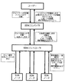
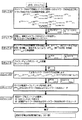
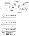
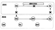
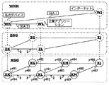
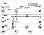
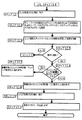
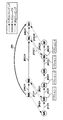
上記の導入に与えられるようにSDNの定義、図1に示すように、以下の成分を含むシステムに、本発明の発明者をリードしています。
1.高レベルのネットワーク仕様でネットワークを定義するユーザ。
2。SDNコンパイラは、物理および仮想ネットワークとコンピューティングリソースのための命令のセットに高レベルのネットワーク仕様を翻訳。
物理および仮想ネットワークとコンピューティングリソースへの命令のセットを配布3. SDNコントローラ。
命令の受信セットに従って着信パケット上のアクションを実行する4.物理および仮想ネットワークとコンピューティングリソース。
図1では、それらは用語「SDNノード」で示されています。
上記の点1に記載したユーザはかもしれないが、人、ネットワーク管理システム、クラウド管理システム、アプリケーション、他のSDNコンパイラが、これらに限定されません。
そのように、ユーザは、スタンドアローンまたはより大きなネットワークの一部であってもよいコンピュータワークステーションのような「ユーザ機器」、すなわち、任意の適切なコンピュータ機器を指すことができます。
このようなコンピュータ装置の例を図31に示し、後述します。
図1では、下から上への方向に、さまざまなコンポーネントは、特定のタスクを実行し、変更、統計情報とエラーを報告してきた彼らのノースバウンドインターフェイスについて報告します。
ポイント4で述べた資源のような典型的なネットワークおよびコンピューティング資源を含むが、これらに限定されません。
・物理パケット転送装置(例えば、ただし中間装置の、レイヤ2スイッチ、レイヤ3ルータ、ファイアウォール、ディープパケット検査装置、キャッシングノード、または他のタイプに限定されません)。
・物理的なサーバ、パーソナルコンピュータ、ラップトップ、タブレット、携帯電話に限定されるものではないようなネットワークホストとして機能する物理デバイス。
・物理ネットワークインタフェースカード(NIC)を。
・仮想化された物理サーバに仮想スイッチ。
・仮想化された物理サーバー内の仮想マシン。
この論理ネットワーク抽象化の仕様は、ユーザにより入力された上記の点1に記載した「高レベルのネットワーク仕様」です。
理想的には、この仕様は、任意の転送ポリシーと任意のトポロジーで論理ノードの任意の数からなる転送パスを 決定し、任意の論理ネットワークを指定し、論理ノードは、任意の物理および仮想ネットワークとコンピューティングリソースにマッピングされています。
複数の論理ネットワークが定義されており、同一の物理および仮想ネットワークとコンピューティングリソース上で同時に作成することができます。
ポイント2は、上記の「ネットワーキングとコンピューティングリソースのための命令のセットに高レベルのネットワーク仕様の翻訳」を指します。
スイッチの場合、これらの命令は、パケットが転送されるべきそれによれば、そのスイッチの転送テーブルエントリです。
ホストの場合、これらの命令は、特定の宛先ノードにそのホストのノードから発信されるパケットを送信するためにどの出力ポートにフィルタテーブルパケットが受け入れまたは削除する必要があり、それによればエントリおよび命令です。
NICの場合、これらの命令は、パケットを転送するのか廃棄する必要があり、それによれば、フィルタテーブルのエントリがあります。
上記に言及ポイント2は、適切な物理および仮想ネットワークとコンピューティングリソースのための命令のセットに高レベルのネットワーク仕様からの翻訳またはコンパイルを提供します。
我々は、低レベルの命令に高レベルの言語を翻訳する、コンピューティングで使用されるコンパイラと同様に「SDNコンパイラのプロセス、このプロセスと呼ばれています。
基本的にの上に仮想的にトンネルを作成します(このようなNicira社/ VMWareの等によって提案されたように)「オーバーレイ」の仮想ネットワークは対照的に、いわゆる、上記のプロセスは、両方の物理および仮想ネットワークとコンピューティングリソースへの指示を提供するべきであることに注意してください物理的なネットワーク、トンネル入口および出口のスイッチを除いて、物理的なスイッチの設定なし。
希望SDNコンパイラの方法は、全体の物理的なネットワークを含む仮想および物理リソースの両方を含む一体的なアプローチを提供する必要があります。
さらに、所望のSDNコンパイラの方法はまた、非スイッチングネットワークデバイスを指示する必要があり、必要な指示を、上記に言及しました。
また、現在のOpenFlowの実装などのソフトウェアで利用可能である(例えば、
オープン仮想化された物理サーバーで実行されている仮想スイッチを提供するvSwitch)と同様に、ハードウェア(例えば
NEC ProgrammableFlow PF5240 スイッチ)、仮想および物理的なネットワークおよびコンピューティングリソースにわたって上記の指示を決定する必要があります。
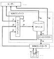
インプリメンテーションでは、「SDNコンパイラ '、または少なくともそれの一部、および「SDNコントローラ」、またはそれの少なくとも一部の機能の機能は、単一のシステムに統合することができます。
論理ネットワーク定義または物理または仮想リソースの変更が発生したときに「SDNコンパイラ」プロセスは、これらの命令の合理的に高速計算を可能にすべきです。
例えば合理的な時間は、LOのミリ秒のオーダーであるかもしれません。
また、転送またはフィルタテーブルのリストには、現在のハードウェアとソフトウェアの実装でサポートされる生産規模ネットワークのための合理的な範囲内に維持されるべきです。
例えば合理的な数の順序エントリは5000転送テーブルエントリの順序になることがあります。
私たちは今、第一の機能表現を使用して、SDNコンパイラは適切な指示を作成するための物理および仮想リソースについて説明します。
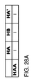
図2A〜図2Gは、物理的なネットワークの構成要素を示しています。
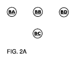
例えば物理ノードは、図2Aに示されている論理ネットワークが作成され、その上に物理的なリソースであると考えられます。
物理ノード(図2AにおけるBDを介してBA)のような名前は、物理リソースを識別するために使用され、任意の時に、転送の決定を行うために使用されていません。
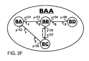
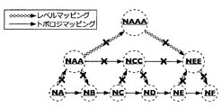
図2(b)に示すように、我々は、物理ノードの集合として(図2bにBAAで識別される)物理的なネットワークを定義します。
物理ノードは、(実線で示す)物理リンクによって相互接続されています。
物理リンクが双方向である場合には、物理 的なリンクは、物理ノードのペア、各方向に1つずつの隣接間の隣接関係のペアを作成します。
物理リンクが単方向である場合には、物理 的なリンクは、物理ノードのペア間の単一の隣接関係を作成します。
物理リンクは、以下を含むが、光ファイバケーブル、銅ケーブル、空気、これらに限定されない、任意の物理媒体とすることができます。
物理リンクもではなく、光波長、時分割多重(TDM)回路、マルチプロトコルラベルスイッチング(MPLS)パスに限定などの他のネットワーク技術、提供するパスすることができます。
物理リンクのセットと組み合わせた物理ノードのセットは、ネットワークの物理トポロジを決定します。
物理的なネットワークは、任意のトポロジーで、その結果、任意のリンクと、ノードの任意の数で構成することができます。
図2Cに示すように、物理ノードと物理的なリンクの間のインターフェースは、p108にpl0lで示される物理的な「ポイントオブアタッチメント」(PoA)、と呼ばれます。
現在展開されたネットワーク内のPoA物理識別子の典型的な例は、イーサネットメディアアクセス制御(MAC)アドレスであるが、我々の発明は、これに限定されるものではありません。
PoAの識別子は、SDNコンパイラの制御下にあるネットワークの集合内で一意である必要があります。
PoAは、パケットがノードから送信された場合、パケットはノードとノードの出力ポート 'で受信されたノードの「入力ポート」の両方を識別します。
図2Dに示されるように、各物理リンクは、一 つまたは複数のコストの種類及び各方向における各原価タイプに関連付けられたコスト値(複数可)を有します。
物理ネットワークで使用される典型的なコストの種類は、典型的にはミリ秒単位のコスト値と、リンクの遅延であるが、コストの任意のタイプを使用することができます。
各双方向物理リンクが2コスト値は、各方向に1つを持っています。
各一方向の物理リンクは、各原価タイプ1のコスト値を有します。
特定の方向における物理リンクのコス ト値は、パケットがその特定の方向のための発信元の物理ノードの最も近くに示されています。
例えばBAからBBへのリンクが1のコスト値を有します。
BBからBAへのリンクが3のコスト値を有します。
物理リンクは、物理ノードの対の間の隣接関係(複数可)を表す一方で、物理的なパスは、ユニキャストネットワークの場合には、物理 的な宛先ノードへのパケットは、物理ソース・ノードから次の物理的経路を表します。
これは、図2Eの一部の例のパスによって示されています。マルチキャストまたはブロードキャストネットワークの場合、単一の物理的なソース・ノードと複数の物理的な宛先ノードの間の物理パスの関係が存在します。
物理パスは、から成る物理リンクの特定の方向の特定のコスト型のコスト値の和に等しく、典型的にはコスト値でそれぞれの方向に複数のコスト・タイプを有することができます。
物理パスは、パケットがソースノードから宛先 ノードに横断するを通じて物理のPoAのシーケンスです。
「パス」の代替用語は、例えば、「フロー」でありますOpenFlowの仕様では、用語「流れ」を使用しています。
一緒に上記の要素を置く、物理ネットワークの典型的な表現は、p108と、各物理リンクのコス ト値を介して物理ネットワークBAA、BDを介して物理ノードのBA、物理の PoA pl0lを示す2Fの図に示します。
転送ポリシーを適用することができるようにするため(例えば、しかし最短パスファーストに限定されない)では、重み付き有向グラフとして、ネットワークを表します。
ネットワークBAAの加重有向グラフは、BDと頂点のペアを接続する有向エッジを介して頂点(ノード)BAを示す、図2Gに示されています。
有向グラフとして表現する場合は、2つの頂点間の双方向物理リンクが2エッジによって表されます。
各エッジは、隣接関係に対応しています。
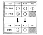
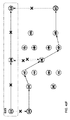
図2Hに示すように、我々は、物理ノードの3タイプを区別:
・物理スイッチノードは、次の機能を持つ:それはソースノードBとなっている、A)の送信パケット)を受信するパケットには宛先ノードCにあるの)着信パケットは、出力のいずれかの入力ポートのいずれかで受信したフォワードD(これを受信したポートを含む)ポート)は、必要に応じてのような、パケットの操作(単数または複数)を提供するが、監視および/または記録および/またはバッファリングおよび/または着信パケット・ヘッダの修正および/またはこれらに限定されませんそれの出力ポートのうちの1つまたは複数にパケットを転送する前に、ペイロード。
また、パケットを(ブロック)転送していません。 e)参照)、パケットFをドロップSDNコンパイラ(オプション)にパケットをカプセル化し、リダイレクト
・次の機能を持つ物理ホストノードに、:A)は、ソースノードBとなっているパケットを送信します)、それが宛先ノードCになっているパケットを受信)パケットDをドロップ)SDNコンパイラ(オプション)にパケットをカプセル化し、リダイレクト
・物理ネットワークインタフェースカード(NIC)は、次の機能では、a)着信パケットが特定の出力ポート(入力ポートと出力ポートとの間の固定された関係)b)のパケットCをドロップ)カプセル化したパケットをリダイレクトするために特定の入力ポートで受信したフォワードSDNへのコンパイラ(オプション)
物理スイッチ、ホストとNICのノードは、図21に示す記号で表されます。
仮想ノードは、以下に説明します。
物理的および仮想ノードのためのSDNコンパイラによる適切な指示を作成することができるようにするために、我々は今、典型的には、現在のネットワークに配置物理および仮想機器をモデル化します。
図3Aは、(例えば、物理的なレイヤ2スイッチ、物理レイヤ3ルータ、ファイアウォール、ディープパケット検査装置、キャッシングノード、または中間装置の他のタイプに限定されない)物理的なパケット転送システムBEを示しています。
物理パケット転送システムは、一つ以上のPoAのp109を有しています。
図3Bに示さ機能表現によって示されるように物理的なパケット転送システムは、物理的なスイッチ・ノードとして表されます。対応する有向グラフを図3Cに示されています。
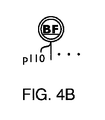
図4Aは、非仮想化コンピューティング装置(例えば、物理的なサーバ、パーソナルコンピュータ、ラップトップ、タブレット、携帯電話に限定されない)BFを示しています。
非仮想化コンピューティング装置は、一つ以上のPoAのp110を有しています。
図4Bに示され、機能表現によって示されるように、非仮想化されたコンピューティング機器は、典型的には、物理 的なホストノードとして使用されています。対応する有向グラフを図4Cに示されています。ホスト・ノードBFは2つのノードに分割されました:図4(c)のノードBFは「受信側ホストを表している一方で、図4(c)のノードBFは、送信側ホストを表しています。
ホストノードは、図2Hごとに、すべての着信パケットを転送することは許されないため、この区別が行われます。ソースパケットを送信し、宛先のパケットを受信するホストノードの機能は、図4(c)に、それぞれ、ノードBF及びBF 'で表されます。
図5Aは、例えば、仮想化されたコンピューティング装置を示しているが、仮想化された物理サーバや仮想スイッチの任意の数に接続された仮想マシンGA-GDの任意の数が作成された仮想化されたブレードサーバ、に限定されるものではなく、仮想化技術を使用して。
仮想化されたコンピューティング機器は、コンピューティング機器外のノードに仮想スイッチBJ、BKからの接続性を提供する、いわゆるネットワークインタフェースカード(NIC)、BG、BHにポアスp111、p112、p114、p115を有しています。
仮想スイッチBJ、BKは、一つまたは複数のNIC BG、BHに接続することができます。単一の仮想マシンGA-GDが(仮想マシンGAおよび仮想スイッチBJによって示される)は、単一の仮想スイッチに接続することができます。
仮想マシンGCおよびGDと仮想スイッチBKによって示されるように、複数の仮想マシンは、単一の仮想スイッチに接続することができます。仮想マシンGBと仮想スイッチBJとBKで示すように、単一の仮想マシンは、複数の仮想スイッチに接続することができます。それぞれ1物理仮想マッピング:N 、N:1、1:私たちは、1としてこれを参照します。
図5Aに示される仮想化されたコンピューティング機器の機能モデルは、図5Bに示されています。物理NIC BG、BHは、図21で定義された記号で表されます。
図21に定義されている仮想スイッチBJ、BKは物理的な転送装置と機能的に同等であるように、仮想スイッチBJ、BKは、物理的なスイッチ・ノードとして表され、物理的なスイッチ・ノードの記号で表されていることに注意してください。
違いは、仮想スイッチとして実装しているBJ、BKは、通常、ソフトウェアではなくハードウェアで実装されています。
仮想マッピングに物理的には、仮想スイッチBJ、BKの仮想マシンGA-GDのポイント・オブ・添 付ファイルを特定の仮想ポアスP 117-P 126と破線で示しています。典型的な実装では、これらのPoAp117、P 126は、典型的には、仮想NICまたはのvNICと呼ばれるが、他の専門用語を使用することもできます。
仮想ポアスパイ17-pl26は仮想マッピングへの物理の物理ノード(仮想スイッチ)と仮想ノードの(仮想マシン)のポイント・オブ・添 付ファイルを識別します。
図6A-6Cは、1の機能的な表現を示す:1、1:NとN:仮想マッピングに物理的に1。
(b)は1を示している図では、仮想マッピングに物理的に1:図6(a)は1を示している仮想マッピングに1物理的に:N仮想マッピングに物理的に、(c)はNを示している把握。
仮想マッピングへの物理的なマッピングの各方向のためのオプションのコスト値を持つことができます。
物理サーバの仮想化の場合、一般的に参照する1に対して行われる:1、1:N、N:1の仮想化は、仮想マシンに物理サーバーの数の比を指します。
1、1:N、N:1は、仮想マシンに仮想スイッチの数の割合を参照している比率1の上方に導入仮想マッピングに物理的にことに注意してください。
図2Hに示すように、我々は仮想ノード、両方とも、仮想マシンの2種類を区別:
・次の機能を持つ仮想スイッチノードに、:A)は、ソースノードBとなっているパケットを送信します)、それが宛先ノードCになっているパケットを受信)出力のいずれかに任意の入力ポートで受信した着信パケットを転送D(これを受信したポートを含む)ポート)は、必要に応じてのような、パケットの操作(単数または複数)を提供するが、監視および/または記録および/またはバッファリングおよび/または着信パケット・ヘッダの修正および/またはこれらに限定されませんそれの出力ポートのうちの1つまたは複数にパケットを転送する前に、ペイロード。
また、パケットを(ブロック)転送していません。 e)参照)、パケットFをドロップSDNコンパイラ(オプション)にパケットをカプセル化し、リダイレクト
上記の仮想スイッチ・ノードがネットワークを可能にする仮想化(NFV)機能:仮想スイッチノードは、トラフィックが転送される介して仮想マシンに実装されています。
上記)Dで述べたように一般的には、仮想スイッチノードは、パケットにオプションの操作を実行します。
・次の機能を持つ仮想ホストノードに、:A)は、ソースノードBとなっているパケットを送信します)、それが宛先ノードCになっているパケットを受信)パケットDをドロップ)SDNコンパイラ(オプション)にパケットをカプセル化し、リダイレクト
物理ネットワークと同様に、我々は、仮想ノードの集合として、仮想ネットワークを定義します。
これは、スイッチの上記特性を持つ仮想マシンを参照するとき、我々は「物理的なスイッチ・ノード」を参照しながら、仮想化された物理サーバー内の仮想スイッチを参照するとき、我々は、「仮想スイッチノード」を参照してくださいすることが観察されます。
また、図5(b)および図6(a)に示されている仮想マシンは、図6(c)は、仮想スイッチノードまたは仮想ホストノードのいずれかとすることができることが観察されます。
このように、スイッチ及びホストノードを表す円記号を表す十字記号は、これらの図では省略されています。
仮想マシンGH、仮想スイッチBR、BS、およびNICのBP、BQは、1つのコンピューティング装置に収容されています。
仮想スイッチBU、及びNIC BTは、別のコンピューティング装置に収容されています。
仮想マシンGJは計算装置の両方のインスタンスに収容されています。
接続の例には、それぞれのポアスpl33、pl53間のリンクを介して表示されます。
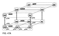
図7Aは、仮想化されたコンピューティング機器のいくつかの追加のプロパティを示しています。
図7Aは、2つの仮想マシンのGH、GJ、3つの仮想スイッチBR、BS、BU、3枚のNIC BP、BQ、BTを示しています。 PoA I 46及びp147で示すように、仮想スイッチは、図7Bの物理リンクによって表される、相互接続することができます。仮想スイッチは、物理スイッチノードによって表されるように、この相互接続は物理リンクで表されることに注意してください。
仮想マシンGJによって示されるように、仮想マシンは、それぞれ異なるコンピューティング装置インスタンス内に存在する複数の仮想スイッチに接続することができます。
冗長性のために、仮想スイッチは、典型的には、複数のNICに接続されています。 NICのリソースおよび他のコンピューティング装置またはパケット転送システムの物理リンクを効率的に利用するために、複数の仮想スイッチは、単一のNICに接続することができます。 NICは今(単一のPoAで識別される)単一の出力ポートへの(複数のPoAで識別される)複数の入力ポートからカプラ/ SPリター転送パケットとして機能し、単一の入力ポートから複数の出力ポートに。
図7aの物理NICは、BPとBQこのカプラ/ SPのトイレの機能を提供するノード:彼らは両方の2つの仮想スイッチBR、BSに接続されています。私たちは、「NICのカプラ/スプリッタ」として、NICのこのタイプを参照してください。
図7Bは、図7Aに示される仮想化コンピューティング装置の機能的な表現を示しています。 NICカプラー/ SP用リターの機能的表現は、NICが全くスイッチング能力を有していないことが観察されたが、入力ポート(S)と出力ポートとの間の固定された関係を提供して、以下に説明されます。
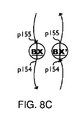
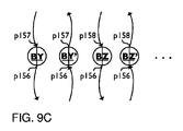
これは、図8A〜図8Cおよび図9A-9Cに示されています。図8Aは、ポアスパイ54パイと55でNIC BXを示しています。
機能モデルは、図8Bに示されています。 POAパイ54で着信パケットは、POAのパイ55に転送されるとのPOAパイ55で着信パケットを受信したPOAパイ54に転送されます。
NICの有向グラフで表現は、図8Cに示されています。 NICノードBXは、その機能性を表すために、図8(c)に2ノードBXとBX」に分割されました:NICノードはどちらの方向に固定された出力ポートに固定された入力ポートからのパケットを転送しています。
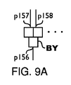
カプラ/ SPリターとしてNIC作用は、図9A-9Cに示されています。 3ポアスpl56、pl57とpl58とBY 2 NICカプラ/ SPのトイレ:図9 Aが1を示しています。
POAパイ56で着信パケットが両方のPoAパイ57とのPoAパイ58に転送される場合には、POA pl57で着信パケットをのPOA pl56に転送される場合には、POA pl58で着信パケットを受信したPOAパイ56に転送されます。
我々は、図9(b)に機能モデルに2つのノードBYおよびBZとして、これをモデル化し、それぞれが、それぞれのPOAパイ56、のPOAパイ57とのPOA pl56、のPOA pl58との間の1対1の転送関係を提供します。
1:NのNICカプラ/ SPのトイレは機能モデルではNの個々のノードになります。
NICカプラー/ sのBPとBQは、図7Bの機能表現のノードBP、BVとBQ、BWで表されているごみノード。ケースではネットワークインターフェイスカードは、物理的なスイッチ・ノードとしてモデル化されるであろう機能を切り替え提供する使用されます。
NICは、コンピューティング機器の境界に位置し、コンピューティング機器内のコンピューティング機器とリソース外部のリソース間の接続を提供します。
図2Hで説明したように、NICは、パケットの送信元または宛先ノードになることはありません。
カプラ/ SPのトイレとしてNIC演技の有向グラフを図9Cに示されています。図のNIC 8 Aと同様に、図9のノードによって表され、BZは今では、BY '、BZ、BZ」ノードで表現されるのカプラー/ SPのトイレとして動作するNIC。
図面2G、3C、4C、8C、9Cに物理ノードの有向グラフ表現が示されています。
有向グラフでまったく同じ表現が仮想と論理ノードは、NIC型ノードではないことをこの例外に、同様に仮想および論理ノードに適用されます。
仮想スイッチノードの能力のような、パケットの操作(単数または複数)を提供する任意に上述のが、パケットを転送する前に、着信パケットのヘッダおよび/またはペイロードの監視および/または記録および/またはバッファリングおよび/または修正に限定されるものではありません一つ以上には、出力ポート、並びにパケット(ブロック)転送ではありません。
今日では、この機能は、典型的には、ファイアウォール、ディープパケット検査デバイス及びキャッシングノードに限定されるものではなく、このようなミドルボックスと呼ばれる専用のハードウェアデバイスによって提供されます。
仮想スイッチノードでこの機能を実現することは、例えば、利益を作成しても減少し、設備コスト、運用コストの削減、ネットワークサービスのより迅速なプロビジョニングに限定されるものではないだろう。
業界では、これは、ネットワーク機能の仮想化(NFV)と呼ばれます。
SDNコンパイラは、仮想スイッチノードに関連する手順を説明します。
NFV機能は、仮想化されたコンピューティング機器に実装された仮想スイッチノードで実現することができました。
上記のように、我々は、機能としてネットワークソフトウェア定義は高レベルの仕様でネットワークを定義するために考慮する(など、しかし、高レベルのプログラミングまたはスクリプト言語に限定されない)を指示し、自動化されたプロセスを介して、適切な物理的及びこの仕様に応じて、仮想ネットワークとコンピューティングリソース。
今では、我々は、物理および仮想ネットワークとコンピューティングリソースの機能モデルを提供してきました。
次に、本発明を例示するために、我々は、高レベルの仕様で定義された物理的および仮想リソースから独立していることができる論理ネットワークを考えます。
論理ネットワークを指定することによって定義されます。
論理ネットワークの1名
論理ネットワークを構成している論理ノードの2名
論理ノード間の3隣接関係
論理ネットワークの4つまたはそれ以上のコストタイプ
各コストタイプのための論理ノード間の論理的な隣接関係の5コスト(複数可)
以下に説明する論理ネットワークの6転送ポリシー、
論理ノードへの物理および/または仮想ノードから7のマッピング
上記で説明し、物理的および/または仮想ノードを使用して、論理ノードにマッピングされ、1:1,1:N、またはN:Lマッピング。
これは以下のように、数字10A-10Gに示されています。
- 図10A:1:1物理論理マッピング
- 図10B:1:N論理マッピングへの物理
- 図10C:N:論理マッピングへリットルの物理
- 図10D:1:論理マッピングに仮想1 - 図10E:1:N個の仮想論理マッピングへ
- 図10F:N:論理マッピングに仮想リットル
- 図10G:N:物理的および論理マッピングに仮想リットル
図1(B)に示されるような論理ノードの機能表現は、破線の円です。論理マッピングの仮想/物理マッピングの各方向のためのオプションのコスト値を持つことができます。
SDNコンパイラのユーザは論理ネットワークを定義します。
ユーザーはかもしれないが、人に、ネットワーク管理システム、クラウド管理システム、アプリケーション、他のSDNコンパイラに限定されるものではありません。
論理ネットワークは、任意の論理トポロジで、その結果、任意の論理的隣接関係で、論理ノードの任意の数で構成することができます。
一例として、論理ネットワークは、論理ノードが各論理ノードの属性であるマッピングされた物理的および/または仮想ノード(単数または複数)と、高レベルのプログラミング言語のグラフのように指定することができます。
論理ノードのために、我々は、物理および仮想リソースの名前空間から独立した論理的な名前空間を使用します。
論理ネットワークは現在、一意の文字の任意の適切な数の任意の適切な形で表現することができ、必要に応じて、適切な仮想および物理リソースにマッピングされる論理ノード名で定義することができます。
このマッピングを変更することにより、論理的なネットワークは、他の仮想および物理リソースに再マッピングすることができます。
1:N個の論理マッピングへの物理的には、複数の論理名を持つ単一の物理リソースに名前を付けることができます。
1:N個の論理マッピングに仮想では、複数の論理名を持つ単一の仮想リソースに名前を付けることができます。
パスは、物理リソースと仮想リソース間に存在し、そのように物理ネットワークと仮想リソースの抽象化を提供して制約を持つもちろん、物理ネットワークと仮想リソースの論理的なネットワークに依存しないことに注意してください。
図11のAに示すように、我々は、論理ノードの2種類を区別:
それがマッピングされている物理的および/または仮想スイッチノードの同じ機能を持つ・論理スイッチ・ノード、。
それがマッピングされている物理的および/または仮想ホストノードの同じ機能を持つ・論理ホストノード、。
図11のAに示すように、論理スイッチ・ノードが論理ノードへの物理的および/または仮想スイッチノード(複数可)のマッピングの結果です。
論理的なホストノードは、論理ノードの物理的および/または仮想ホストノード(複数可)のマッピングの結果です。
物理NICが論理ネットワーク内のエンティティにマップされていません。
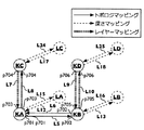
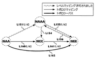
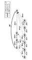
ノードの種類と記号の完全なリストは、図1(B)にまとめられています。ノードの上のモデリングは3パケット転送システム、DB、DC、DD、仮想スイッチDA、NICのDE及びDFおよび仮想マシンのHAとHBとで1仮想化されたコンピューティング機器からなる、図12に示すネットワークのモデル化によって示されています一つの非仮想化されたコンピューティング機器DG。
パケット転送システムDBは、パケット転送システムDCでのPOA P77へのPOA P75にあるリンクを介して接続され、パケット転送システムDDでのPOA P78へのPOA P74でリンクを介しています。パケット転送システムDBは、コンピューティング機器の物理NIC DFののPOA P80へのPOA P73にあるリンクを介して接続されています。
パケット転送システムのDCは、コンピューティング機器の物理NICのDEのPOA P82へのPOA P76にあるリンクを介して接続されています。
パケット転送システムDDは、コンピューティング機器のDGでのPOA P84へのPOA P83にあるリンクを介して接続されています。仮想スイッチDAが物理NICのDEでのPOA P81へのPOA P72にあるリンクを介して接続されています。仮想スイッチDAも物理NICのDFでのPOA P79へのPOA P71にあるリンクを介して接続されています。
仮想マシンのHAは、仮想スイッチのDAでのPOA P85へのPOA P86にあるリンクを介して接続されています。仮想マシンHBは、仮想スイッチのDAでのPOA P87へのPOA P88にあるリンクを介して接続されています。
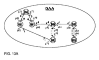
すべての物理ノードの機能的表現は、上記で説明したアプローチによれば、図13のAに示されています。
図13のAでは、様々なリンクの重みは、双方向リンクの各方向のために追加されました。
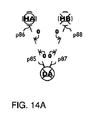
これらの物理的なノードの集合は、物理的なネットワークDAAと呼ばれています。仮想スイッチDAは、図13Aのネットワークの重み付き有向グラフ表現は図13bに示されている図13 Aの機能的表現で物理スイッチ・ノードであることに注意してください。図14Aは、ネットワークDAA内の仮想マッピングにのみ物理的である物理ノードDAおよび仮想ノードHAとHBの間の仮想マッピングに物理的に描いています。 P88を通じてポアスP85は、仮想のPoAであることに注意してください。また、両方のマッピングのコストは両方向でゼロであることに注意してください。
仮想マシンHBが仮想スイッチノードの機能を提供しながら、ここでの例では、仮想マシンのHAは、仮想ホストノードの機能を提供します。
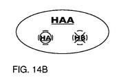
我々は、図14Bに示されるように、仮想ネットワークHAAなどの仮想ノードHAとHBのコレクションを参照してください。私たちは、仮想および物理リソース上に論理ネットワークのマッピングを説明するために、この例を使用します。
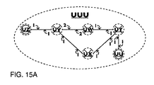
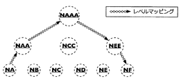
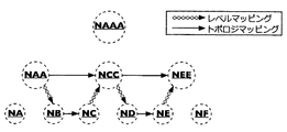
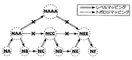
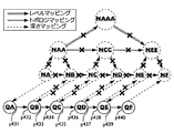
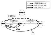
図15Aは、論理ノードUU、UV、UW、UX、UYとUZからなる、例えば論理ネットワークUUUを示しています。論理ノードの名前は、上に転送決定を行うために使用されます。
ないそのインターフェイス、論理ノード自体に名前が付けられていることに注意してください。
物理ネットワークとの類推では、論理ノードの集合として(図15 Aでは、UUUで識別)論理ネットワークを定義します。
論理ノードは、(実線で示す)論理リンクによって相互接続されています。
論理リンクが双方向である場合、論理リンクは、論理ノードのペア間の隣接関係のペアを作成します。
論理リンクが単方向である場合、論理リンクは、物理ノードのペア間の単一の隣接関係を作成します。
論理リンクのセットと組み合わせ論理ノードの集合は、ネットワークの論理トポロジを決定します。
各論理リンクは、一 つまたは複数のコストの種類と各原価タイプに関連付けられたコスト値(複数可)を有します。
各双方向論理リンクは、それぞれのコストタイプ、各方向に1つずつ2コスト値を持っています。
各一方向の論理リンクは、各原価タイプ1のコスト値を有します。
特定の方向における論理リンクのコス ト値は、パケットがその特定の方向のための発信元の論理ノードの最も近くに示されています。
論理リンクは、論理ノードの対の間の隣接関係(複数可)でありながら、論理パスは、ユニキャストネットワークの場合には、論理的な宛先ノードへのパケットは、論理ソース・ノードから次の論理的な経路を示しています。
マルチキャストまたはブロードキャスト・ネットワークの場合には単一の論理ソースノード及び複数の論理的な宛先ノードとの間の論理パスの関係が存在します。
論理パスは、から成る論理リンクの特定の方向の特定のコスト型のコスト値の和に等しく、典型的にはコスト値でそれぞれの方向に複数のコスト・タイプを有することができます。
論理パスは、物理のPoAおよび/またはパケットが論理的な宛先ノードへの論理ソースノードから横断する介して仮想のPoAのシーケンスです。
論理ソースと論理宛先ノードと物理と仮想のPOAのの観点から説明パスとの関係:ここでは、重要な関係に到着しました。
これは、私たちは物理的および/または仮想ネットワークおよび/またはコンピューティングリソースのための物理的および/または仮想のPoAの点で命令に定義されているネットワークを論理ノード名にネットワークを定義し、翻訳(コンパイル)することができます。
論理ネットワークUUUの加重有向グラフ表現は、図15Bに示されています。論理ノードの物理的および仮想ノードとの間のマッピングは、図15Cに示されています。仮想/物理ノードと論理ノード間のすべてのマッピングのコストがゼロであることに注意してください。
図16は、図12、13 A、13B、14A、14B及び15A-15Cに示された例のための物理的、仮想的、論理ノードと物理的および論理的なネットワークとの間の関係をまとめたものです。図16の物理ネットワークDAAの下部に表示されます。
示すように、物理ネットワークDAAは、その物理リンクおよび物理のPoAでDGを介してノードのDAを含みます。
HA(仮想ホストノード)とHB(仮想スイッチノード)という名前の2つの仮想マシンが物理ノードDAにマッピングされている(1:仮想マッピングに物理的に2)。
1物理的および/または論理マッピングに仮想:論理ノードUU、UV、UW、UX、UY、UZは1を介して、それぞれ物理ノードDG、仮想ノードHB、物理ノードDB、DC、DDと仮想ノードHAにマッピングされます。
私たちは、「論理マッピングに対する仮想/物理」として物理的および/または論理マッピングに仮想を参照します。
論理ネットワークUUUは、図15に示すように、論理ノードが論理リンクとUZを通じてUU含みます。
物理NICのノードは、ソースノードまたはそれが宛先ノードになっているパケットを受信して いるのパケットを(図2Hを参照)を送信しないように、論理マッピングの仮想/物理的には、NICのノード上で実行することができません。
したがって、ノードDEとノードDFは物理NICのノードである、論理マッピングの仮想/物理的には、ノードとノードDE、DFのために行われません。論理マッピングの仮想/物理的には物理ノードのDAに行われないことに注意してください。これは、この特定の例のための選択である、また、物理ノードDAの論理マッピングに仮想/物理が行われている可能性があります。これは、論理マッピングの仮想/物理的には必ずしも物理的または仮想スイッチまたはホストノード上で実行される必要がないことを示しています。
比較的簡単な例を維持するために論理マッピングに仮想/物理1:この例では、1つだけを示しています。
同様に1:NまたはN:1論理マッピングの仮想/物理が使用されている可能性があります。
一般的には、論理ネットワーク内のノードの数は、それがマッピングされた数の物理および仮想ノードから独立しています。
論理マッピングの仮想/物理1:論理ネットワークUUUのトポロジーがあっても1でマッピングされているノード間で物理的なネットワークDAAのトポロジーとは異なることに注意してください。
例えば物理ノードDBと物理ネットワークDAA内の物理ノードのDCとの間のリンクがある間は論理ノードUWはUXはある物理ノードDBと論理ノードにマッピングされている間に論理的なネットワークでUUUは、論理ノードUWと論理ノードUXの間にはリンクが、ありません物理ノードDCにマッピングされました。物理ネットワークDAA内の物理ノードのDCと物理ノードDDとの間にリンクがないながら、論理ノードUXは、物理ノードDCおよび論理ノードにマッピングされている間も、論理ネットワークUUUで論理ノードUXおよび論理ノードUYとの間のリンクは、そこにありますUYは、物理ノードDDにマッピングされています。論理ネットワーク内のリンクは、物理ネットワーク内のリンクと物理から仮想ノードへのマッピングから独立している:これは、論理ネットワークの重要な特性を示しています。
また、論理ネットワーク内の隣接関係のコストは、物理ネットワーク内の同じ隣接関係のコストと異なることがあります。
これは、物理ネットワークに指定された転送ポリシーとは異なる論理ネットワーク内の特定のパスに沿ってパケットを転送することができます。
これは、論理ノードUV及び論理ノードUW(参照する図15B)との間のリンク上の両方向に2のコスト値を使用して示されています。
物理ネットワークに指定された転送ポリシーとは異なる論理ネットワーク内の特定のパスに沿ってパケットを転送する機能は、仮想スイッチ・ノードに作用する仮想マシンのような、パケットの操作(複数可)を提供するために使用されたときに非常に便利ですしかし、着信パケットのヘッダおよび/またはペイロードの監視および/または記録および/またはバッファリングおよび/または修正に限定されない、または(ブロッキング)パケットを転送しません。
論理ネットワーク内の隣接関係のための適切なコスト値を選択し、論理ネットワーク内の転送ポリシーを適用することにより、パスが転送以外の特定の機能を実行する仮想スイッチ・ノードとして動作する特定の仮想マシンを横断論理ソースと論理宛先ノード間に作成することができますパケットに。
完全を期すために、我々は、物理、仮想、および論理的な要素をまとめたものです。
物理的要素:
- 物理的なネットワーク
- 物理的なスイッチ・ノード
- 物理ホストノード
- 物理NICノード - 物理のPoA
- 物理リンク
- 物理パス仮想の要素:
- 仮想ネットワーク - 仮想スイッチノード
- 仮想ホストノード
- 仮想のPoA論理要素:
- 論理ネットワーク - 論理スイッチノード
- 論理ホストノード
- 論理リンク - 論理パス
ネットワーク内の隣接関係やネットワーク内のパスの間の関係は、特定のネットワークの転送ポリシーによって決定されます。
本質的には、ネットワークの転送ポリシーは、転送パスのセットに、ネットワーク内の隣接関係の翻訳を提供します。
ネットワークで使用される典型的なポリシーの例としては、これらに限定されないが、以下のとおりです。
・最短パス優先(SPF)
・ファイアウォール(パスが許可されません)
・指 定されたパス(パス内のすべてのノードを指定します)
・ロードバランシング
複数のポリシーは、全体のポリシーにまとめることができます。
我々は論理コンポーネントの面でネットワークを定義すると、パケット転送の決定は、論理ノード名に基づいて行われます。
物理的および仮想ノードは、物理リソースと仮想リソースを識別する目的のためだけに名前が付けられています。
転送の決定に使用する物理または仮想ノード名があることはありません。
図17は、パケット転送システム内のパケット転送を示しています。
ここで、出力ポート=フォワーディング関数f(論理ソースノード、論理的な宛先ノード、入力ポート、ロードバランシング識別子):パケット転送は次のように記述されています。
- 転送関数f:フォワーディングテーブルに対してルックアップが提供するローカルフォワーディング機能(複数可)
- 論理ソースノード:着信パケットのヘッダに記載されているようにパケットは、発信された論理ノード。
- 論理的な宛先ノード:着信パケットのヘッダに記載されているように、パケットが、宛先とされた論理ノード。
- 入力ポート:パケットが転送ノードを入射する物理または仮想のPoA
- 出力ポート:パケットが転送された物理または仮想のPoA。 - ロードバランシングの識別子:ロード・バランシングの目的のために、オプションの識別子。
転送テーブル内の各エントリには含まれています:論理ソースノード、論理的な宛先ノード、入力ポート、オプションのロード・バランシング識別子、出力ポートを。
ケースでは、特定の要素は、転送の決定(例えば、論理ソースノード) '*'(アスタリスク)には関係ありません、ワイルドカード記号として使用されています。
「転送テーブル」の代替用語は、「フローテーブル」であり、例えばOpenFlowの仕様では、用語「フローテーブル」を使用しています。
ユニキャストの場合、各エントリは、パケットが転送された単一の出力ポートを指定します。
マルチキャストまたはブロードキャストパケットの着信の場合は、複数の出力ポートに転送されます。
ローカルフォワーディング関数fに転送する論理ノード名(論理ソースノード、論理的な宛先ノード)との物理的および/または仮想出力ポートとの間の関係を提供します。
それは、物理および仮想の出力ポートに変換する、論理コンポーネントの面でネットワークの定義と作成を可能として、この関係は非常に重要です。
また、パケットがドロップすることができますまたは必要に応じてSDNコンパイラにカプセル化し、リダイレクトすることができます。
我々が検討しているノードの3つの異なるタイプ、すなわちスイッチノードは、ホストノードとNICのノードの転送動作は、それぞれ、図18A、図18B、図19、図20A-20Cに示されています。
図18のAに機能を備えた物理または仮想スイッチノード描いている:A)は、転送機能FBに基づいて出力ポートのいずれかにソースノードとなっているパケットを送信する)それが基づいて宛先ノードになっているパケットを受信転送機能FC)は転送関数fに基づいて、それを受信したポートを含む出力ポート()のいずれかの入力ポートのいずれかで受信した着信パケットを転送します。
ケースでは一致するものが転送テーブルにパケットがドロップされ、および/または必要に応じてカプセル化され、SDNコンパイラにリダイレクトされるルックアップ見つかりません。
図18Bは、図18Aのスイッチ・ノードの機能を提供するスイッチ・ノードを示し、
さらに能力:d)任意にパケットを転送する前に、監視および/または記録および/またはバッファリングおよび/または着信パケットのヘッダおよび/またはペイロードの修正に限定されたパケットの操作(単数または複数)を提供する、などではなくそれのうちの1つ以上は、パケットを(ブロッキング)転送出力ポートまたはではありません。
これは、図18Bにオプション機能」と呼ばれています。スイッチ・ノードは、複数のオプション機能を実行することができます。
A)であるが注意してくださいとパケットが転送されていない上にb)は、我々はまだを参照するために、単一の機能を持つように、「転送機能」を参照してください。
A)は、転送機能Fに基づいて出力ポートのいずれかにソースノードとなっているパケットを送信します。図19は、する能力を持つ物理または仮想ホストノードを示しています
B)は転送関数fに基づいて、宛先ノードであるパケットを受信します
ケースでは一致するものが転送テーブルにパケットがドロップされ、および/または必要に応じてカプセル化され、SDNコンパイラにリダイレクトされるルックアップ見つかりません。
物理または仮想ホストノードは、パケットの任意の転送を提供していません。
しかし我々は関係なく、ノードタイプのこの関数の命名で一致するように、ホストノードの場合、転送機能として関数fを参照します。
ホストノードの場合、転送関数fは、特定のノードを宛先ホストノードから発信出力ポートパケットが送られるべきであることを指定します。
また、それは、着信パケットを受信したか、削除するかどうかを指定します。
20 A、20Bが図、図20Cは、着信パケットを転送する物理NICのノードは、入力ポートと出力ポートとの間に固定された関係で、特定の出力ポートに特定の入力ポートで受信示します。
1、図20B 1:Nお よび図20C、N:1の関係図20Aは、1を示しています。
パケットは基本的に、NICの場合のフィルタテーブルでフォワーディングテーブルに従って転送されます。また、パケットがドロップすることができますまたは必要に応じてSDNコンパイラにカプセル化し、リダイレクトすることができます。
実装では、いくつかのノードは、機能が制限される可能性があります。
例として、NICがパケットをカプセル化し、SDNコンパイラにリダイレクトする能力を持っていない可能性があります。
これは、システム全体に少ない機能を提供しますが、これは作業の実装です。
また、一例として、NICは、パケットをフィルタリングする機能を持っていないかもしれないと、パケットヘッダ内の宛先アドレス、入力ポートおよび/またはオプションの負荷が識別子のバランスをとるパケットヘッダに関係なく、送信元アドレスのすべてのパケットを転送します。
これは以下のセキュリティになりますが、これは作業の実装です。
また、一例として、ホストは、すべてのSDNコンパイラによって作成された転送テーブルをサポートしていますが、すべての着信トラフィックを受信し、単一の出力ポート(POA)のすべてのトラフィックを送信しない場合があります。
SDNコンパイラでこの単一のPOAにこのホストのモデル化、作業の実施になります。
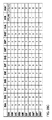
SDNコンパイラによって実行されるメソッドを作成するために、上記のモデルは、現在の行列に関して説明されています。
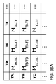
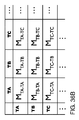
我々は、次の6マトリックスタイプを区別:
- で表されるPOAに隣接行列<PoAの>:のPoAで表し、ノード間の隣接関係を記述
記述転送(パス)のPoAで表し、ノード間の関係を: - F <PoAの>で示されるPOAに転送行列
- Mで表されるPOAにマッピング行列<POAは>:ノード間のマッピング関係を記述するのPoAで表現
隣接コスト値で表し、ノード間の隣接関係を記述: - <OS>で示されるコスト値を持つ隣接行列
- F <費用>で示されるコスト値と転送行列:記述転送(パス)は、ノード間の関係は、パスコスト値で表現
マッピングのコスト値で表現さのノードとの間のマッピング関係を記述する: - M <費用>で示されるコスト値とのマッピング行列
私たちは、POA型マトリックスなどの最初の3つの行列を参照してください。
我々はコスト型マトリックスなどの、最後の3つの行列を参照してください。
すべての行列は、行と列を持っていると行(インデックスi)および列(インデックスj)方向の両方にノード名によってインデックスされています。
インデックスjは行列が表す隣接、パスまたはマッピング関係に宛先ノードを示しているインデックスiがソース・ノードを示します。
隣接行列の場合は、転送行列の場合の行と列は、ノードの同じセットによってインデックス付けされています。
行のインデックスを作成するノードの順序は、しかし、列のインデックスを作成するノードの順序と異なる場合があります。
マッピング行列の場合は行のインデックスを作成するノードのセットは、どちらかと異なることや列のインデックスを作成するノードのセットと同じにすることができます。
PoAの型隣接および転送行列の一般的な表現は、行列の各要素は、それぞれの行にして、1つ以上の行が含まれている図21 Aに描かれているフォームの出力ポートののPoA(入力ポート)の配列。 。 。」任意の長さの。
PoAの型隣接行列の場合は、のPoAのこのシーケンスは、列jによって索引付けノードに行iでインデックス付けノードから隣接関係を示しています。
要素I、Jの複数の行にあるノードiとノードjの結果との間に複数の隣接関係は、それぞれが隣接関係を表します。
ケースでは全く隣接iは、iとノードjのノードとの間に要素の値を存在しない、のPoA型隣接行列でjは0(ゼロ)です。
ノードは、自身と隣接関係を持っていない場合には、当該PoA型隣接行列の対応する要素の値が0(ゼロ)です。
PoAのタイプの転送行列の場合には、のPoAのこのシーケンスは、宛先ノードjへのIソースノードからの経路を表します。
要素I、Jの複数の行にあるノードiとノードjの結果との間に複数のパスは、それぞれがパスを表します。
ケースでは全くパスは、ノードiとノードj、i、jが0(ゼロ)要素の値の間に存在しません。
自分自身に得るためにノードに必要な一切のパス、セル、iの対応する値がないので、場合指標でjはiと指数jは、POA型の転送行列の同じノードをしている識別値1(1)、何も出力がないことを示しますポート(入力ポート)が必要とされています。
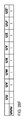
隣接のPoA型マトリクスの例は、図27Bおよび図29Bに示されています。転送のPoA型マトリックスの例を図27D及び29Cに示されています。
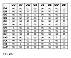
PoAの型マッピング行列の一般的な表現は、図22Aに示されています。マッピング文は、次の値のいずれかが含まれます。
- フォームの出力ポート(入力ポート)ののPoAの各行の配列と1つまたは複数の行、。 。 。」任意の長さの。
- 1(1)
- 0(ゼロ)
値出力ポート(入力ポート)。 。 。 「出力ポートと、行iおよび列jによってインデックス付けノードによってインデックス付けノード間のマッピングを示している 'ノードのiとノードjの「入力ポート」。
値が '1' iとノードが指定した任意のPoAなしに、列jによって索引付け行によってインデックス付けノード間のマッピングを示しています。値が「0」の行によってインデックス付けノードiとj列によって索引付けノード間のマッピングを示していません。
PoAの型マッピングマトリックスの例を図28B、28C、28G、28Hに示されています。 PoAの型マトリックスはコスト型行列を伴っています。
コスト型行列の行と列のインデックス付けは、対応のPoA型行列の行及び列の索引付けと同じです。
コスト型隣接および転送行列の一般的な表現は、図2(B)に示されています。隣接コストマトリックスは、それが付属して隣接のPoA行列で指定された隣接関係のコスト値が含まれています。
各POA型隣接行列は、特定のコストタイプを表す1つ以上の添付コスト型の隣接行列をそれぞれ持つことができます。
ケースでは隣接関係は、ノードiとノードj、コスト型隣接行列 ∞される(無限大)の要素I、Jの値の間に存在していません。
要素の複数の行にあるノードiとノードjの結果との間に、複数の隣接I、J iの要素、それは付属のPoA型隣接行列のJで特定の行に対応するコスト値を表す各。
ケースでは、ノードは、自身との隣接関係、コストタイプ隣接行列∞される(無限大)の対応する要素の値を持っていません。
転送コストマトリックスは、付属の転送のPOA行列で指定されたパスのコスト値が含まれています。
各々のPoA型転送行列は、一つ以上の付随するコスト型の転送行列特定のコストタイプを表すそれぞれを有することができます。
ケースでは何のパスは、ノードiとノードj、コスト型の転送行列∞される(無限大)の要素I、Jの値の間に存在していません。
要素I、Jの複数の行にあるノードiとノードjの結果との間に複数のパスは、それぞれがiの要素、それは付属PoA-タイプの転送行列のj内の特定の行に対応するコスト値を表します。
自分自身を取得するノードのために必要なパスが存在しないため、コスト型の転送行列の対応する要素はゼロのコストを示す、0(ゼロ)です。
隣接コスト型マトリクスの例は、図27Cおよび29Aに示されています。転送コスト型マトリックスの例は、図27E及び29Dに示されています。
コスト型マッピング行列の一般的な表現は、図22Aに示されています。各POA型マッピング行列は、特定のコストタイプを表す1つ以上の添付コスト型のマッピング行列をそれぞれ持つことができます。
マッピング文は、次の値のいずれかのいずれかが含まれています - 各行コスト値をオンにした1つまたは複数の行、
-∞(無限大)コスト値は、iとノードはコスト値が特定のコストマッピング行列が表す特定のコストタイプのコスト値であることと、列jによって索引付け行によってインデックス付けノード間のマッピングを示しています。
コスト値が無限大にすることはできません。
コストオートディーラーステートメント値「∞」(無限大)は、行によってインデックス付けノードiとj列によって索引付けノード間のマッピングを示していません。
コスト型マッピングマトリックスの例を図28Dに、28E、281、28Jに示されています。
マッピングマトリックスの別の型は、ノードとネットワークとの間のマッピングを提供するだけでなく導入されます。
マッピングマトリックスのこのタイプの一般的な表現は、図22Bに示されています。マトリックスのこのタイプの単一の行には、ネットワーク名をインデックスされ、列(インデックスj)は、1つまたは複数のノード名によってインデックスされています。
要素の値は、I、Jは次のとおりです。
- 1(1)jでインデックス付けノードがネットワークiの一部である場合には
- 0(ゼロ)jでインデックス付けノードがネットワークiの一部ではない場合には
我々は、ネットワークマッピング行列として、このマトリックスを参照します。
ネットワーク・マッピング行列は、POA型の行列です。
ネットワークノードとの間のマッピングマトリックスの例は、図27A、28A〜28Fに示されています。
上記のマトリックスで実行されます主な操作は行列であります
乗算。
動作は、第1の行列の行の要素を第2の行列の列の対応する要素で乗算されている標準的な行列の乗算、との類似性を有します。
PoAの型及びコスト型の行列で行列乗算は、図23A-23H及び24A-24Mに説明されます。行列の乗算に関わる行列は、同じタイプのPoAの型またはコスト型行列のいずれかである必要があります。
我々は最初のPoA型行列の行列乗算を考えます。
二つの行列RRAとRRBは、それぞれ図23のAおよび23 Cで定義されています。
行列乗算を説明する目的のために、これらの行列を使用することができるが、行と列の任意の数の一般的なマトリックスにおける3×3の行列です。
行列の乗算で第1の行列と第2のマトリックスの行の列の数が同じであるべきであり、同じ順序でのノードの同じセットによってインデックス付けされます。
マトリックスRRAは、POA型行列であり、行列がRRBのPoAタイプの行列です。
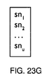
RRAの各要素は、「SA」のq列からなる要素の図23Cに示されるように「SB」r行からなる素子に図23Dに示されるように「SC」要素の図23Bに示されるように1つまたは複数の行で構成され行からなります。
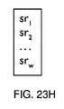
RRBの各要素のu列からなる要素の図23Fに示されるように、1つ以上の行で構成され「SK 'T行からなる、要素の図23Gに示すように、「SN」、要素については、図23Hに示すように、「SR」 W行から成ります。
ケースでは要素が2列以上で構成され、これらの行のいずれかの値が0(ゼロ)にすることはできません。
行列乗算RRC = RRA <> RRB(このセクションで定義されたようなマトリックス乗算演算を示す・ここで)図24Aに示されたマトリックスRRCで結果。基本的に、標準的な行列乗算処理が使用されている第1の行列の行の要素は、第2のマトリックスの列の対応する要素と乗算され、標準的な行列乗算操作の結果の要素の乗算は、に変更しました「**」操作と標準の行列演算に起因する要素の合計は、新しい行が生じています。
行列RRCの要素の最初の行(RR、RX)は「SA ** SK」です。
操作「SA ** SKが「図24Bに示される行要素の結果です。本質的には、「SA」の様々な行ののPoAの配列は、すべての可能な組み合わせの「SK」の様々な行ののPoAのシーケンスによって追加されます。
同様に、2行目「SB ** SN 'および3行目「SC **、SR'要素のRRC(RR、RX)とを算出します。
行列RRCの「SA ** SK '、SB ** SN」と「SC ** SR'要素については、図24Cに示されるように、すべての行からなる単一の要素に結合されている(RR、RX)の結果行。場合にRRAまたはRRBの行列要素の値が0(ゼロ)が含まれ、このマトリックス要素を伴う「**」操作中のオペランドの一方が0(ゼロ)です。
「**」操作中のオペランドの一方が0(ゼロ)である場合、値0(ゼロ)と一列に「**」の演算結果。
結果の行列要素は、行列要素が単一に設定されている場合、これらのすべての行の値が0(ゼロ)、1つまたは複数の行で構成されない限り、すべての値が0(ゼロ)は、行列乗算の結果の行列から除去され値0(ゼロ)の行。
場合RRAやRRBの行列要素が値1(1)が含まれ、この行列要素を伴う「**」の操作でオペランドの一方は、1(1)です。
「**」の操作でオペランドの一方が1(1)である場合には、他のオペランドの値に「** '演算結果。
値1(1)と「SA」の任意の行について、その行を含む「SA ** SK」の結果の値は「SK」の各列の値に等しいです。
値1(1)と「SK」の任意の行について、その行を含む「SA ** SK」の結果の値は「SA」の各列の値に等しいです。
この場合、図24Dに示されている「SAI」は値1(1)があります。
コスト型マトリックス上で行わ行列乗算演算は、図23A-23Hと24E、24F、24Gに説明されます。図23A及び23Cで行列RRAとRRBはそれぞれ今コスト型行列です。
これらの行列は、3×3行列である行列乗算を説明する目的のために、しかし、一般に、行と列の任意の数のマトリックスを使用することができます。
行列の乗算で第1の行列と第2のマトリックスの行の列の数が同じであるべきであり、同じ順序でのノードの同じセットによってインデックス付けされます。
行列RRA原価型行列であり、行列は、RRBコスト型の行列です。
RRAの各要素は、「SA」のq列からなる要素の図23Cに示されるように「SB」r行からなる素子に図23Dに示されるように「SC」要素の図23Bに示されるように1つまたは複数の行で構成され行からなります。
RRBの各要素のu列からなる要素の図23Fに示されるように、1つ以上の行で構成され「SK 'T行からなる、要素の図23Gに示すように、「SN」、要素については、図23Hに示すように、「SR」 W行から成ります。
ケースでは要素が2行以上で構成され、これらの行のいずれかの値がbe∞(無限大)することはできません。
行列乗算RRD = RRA <> RRB(このセクションで説明する行列乗算演算を示す・ここで)図24Eに示されたマトリックスRRDで結果。基本的に、標準的な行列乗算処理が使用されている第1の行列の行の要素は、第2のマトリックスの列の対応する要素と乗算され、標準的な行列乗算操作の結果の要素の乗算は、に変更しました「++」操作と標準の行列演算に起因する要素の合計は、新しい行が生じています。
行列RRDの要素の最初の行(RR、RX)は「SA ++ SK」です。
操作は「SA ++ SK」の図24Fに示されている行要素が得られています。本質的には、「SA」の様々な行のコスト値は、すべての可能なにおける「SK」の様々な行のコスト値に加算されます
組み合わせ。
同様に、RRDの2行目「SB ++ SN 'と3行目「SC ++ SR'要素の(RR、RX)を算出しています。
行列の要素(RR、RX)については、図24Gに示すように、「SA ++ SK」、「SB ++ SN」と「SC ++ SR」の結果の行は、すべての行からなる単一の要素に結合されますRRD。場合RRAやRRBの行列要素は値∞(無限大)、この行列要素 ∞される(無限大)を含む「++」の操作でオペランドの一方が含まれています。
「++」操作 ∞される(無限大)でのオペランドの場合には1、値∞を持つ単一の行に「++演算結果(無限大)。
結果の行列要素は、行列要素は単一の行に設定されている場合、すべての行の値∞(無限大)、1つまたは複数の行で構成されていない限り、すべての値∞(無限大)は、行列の乗算から生じる行列から削除されます値∞(無限大)と。
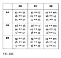
我々は、図24Hの例物理的なネットワークを使用して行列の乗算を示しています。物理ネットワークCAAは、物理スイッチノードCH、CJ、CK、CLで構成されています。仮想ネットワークGAAは、仮想スイッチ・ノードGR、GS、GTの、この例では、構成されています。図に示されるように物理的なスイッチ・ノードCJが仮想スイッチノードのGSとGTにマッピングされている間に241物理スイッチノードCHは、仮想スイッチノードGRにマップされます。物理ネットワークCAAの隣接行列は、我々は、F <POA> CAAと呼ぶ図24Kに示されている物理ネットワークCAAの<POA> CAA転送行列と呼ぶ、図24Jに与えられています。
最初の最短パス優先(SPF)のポリシーは、図24Hに示される隣接コスト値を使用して適用されています。第二に、追加のパスはノードCJを通じてCHをノード間CJを通じて、ノードCKからのCKをノード間CHから作成されています。これらの追加のパスは、それぞれの要素(CH、CK)とCAAの転送行列の要素(CK、CH)の2行目になります。
我々はM <POA> GAA-CAAは、図24Lに示すように参照する物理ノードのCH、CJ、CK、CLに仮想ノードGR、GS、GTからのPoA型マッピング行列。適用行列の乗算M <POA> GAA-CAA * F <POA>図24Mに示すマトリックスにCAA結果。この行列は(CH、CJ、CK、CL)の物理ノードに仮想ノード(GR、GS、GT)からのすべてのパスを提供します。
仮想ノードGRと物理ノードCKとの間に2つのパス内の物理ノードのCHおよびCK結果との間に2つの経路があり ます。 ' - '細胞内のシンボル(GR、CK)及び(GR、CLは)のPoAのシーケンスが次の行に続くことを意味します。
本質的には、PoAの型行列の行列乗算はのPoAで表さネットワーク内のパスを作成しています。関連するコスト型行列の行列乗算はコスト型行列が表す特定のコストタイプのためにそのパスのコストを作成しています。
単一の物理ネットワーク、単一の仮想ネットワークと単一の論理ネットワークのSDNコンパイラ方法の詳細な例を図25に示されています。
ステップ1:
ネットワークAAAは物理的なスイッチ・ノード、ホストノードとの物理リンクによって相互接続されたNICのノードを構成する物理ネットワークです。
物理ノード名、物理ノードタイプ(スイッチ、ホスト、NIC)、物理リンク、物理のPoA、必要に応じて各コストタイプkに対する物理リンクコスト、仮想のPoA、仮想の物理ノードからの方向に仮想マッピングへの物理の必要に応じて費用各コストタイプkのノードが検索され、物理的なネットワークのAAAのために記憶されます。実装によっては、この情報は、SDNコントローラ、直接ノード、ネットワーク管理システム、ネットワークオペレーションシステム、クラウド管理システム、他の手段またはこれらの組み合わせから取得することができます。
ケースではコストタイプは、その値は通常の測定から取得され、「待ち時間」です。
他のコスト・タイプの場合には、その値は、典型的には、オペレーションシステムに定義されています。
私たちは、ネットワークのAAAとAAAが含まれているノードのネットワークとの関係をMAAA提供ネットワークマッピング行列を定義します。
私はネットワークのAAAと彼らは加重有向グラフ表現で表現されるように、我々はノードを使用したAAAのノードによってインデックス付け一つまたは複数の列jでインデックス付け単一の行からなるMAAA。
NICおよびNICノード:したがって、MAAAa NICに2つのノードで表されます。
ホスト:MAAAaでホストが2つのノードで表され、
(送信ホストを表す)と、(受信側ホストを表す)ホスト」。
MAAAであります 1(1)のすべての行列要素の値。
図16のネットワークDAAのネットワークマッピングマトリックスの例を図27Aに示されています。
手順2:
手順1で取得した情報に基づいて、物理的なネットワークのAAA AAAof単一のPoA型隣接行列A <POA>が作成されます。
一つ以上の添付コスト型隣接は<コストのK> AAAありますが作成し、それぞれのコストタイプkの1行列します。
図16のネットワークDAAのためのそれぞれPoA-タイプの隣接行列とコスト型の隣接行列の例は、それぞれ、図27Bおよび27Cに示されています。
ステップ3:
上記のように、ネットワーク内の隣接ネットワーク内の経路間の関係は、特定のネットワークの転送ポリシーによって決定されます。
私たちは、フォワーディングポリシーPAAAofネットワークAAA、ネットワークのAAAでの転送パスのセットにネットワークのAAAでの隣接関係の翻訳を提供し、基本的に関数を定義します。典型的な転送ポリシーの例は、以下のステップ4の説明に記載されています。
ステップ4:
物理ネットワークのAAA AAAof単一転送のPoA行列F <POA>が作成され、物理的なネットワークのAAA内のすべてのパスを含む5は、物理のPoAで表現。図16のネットワークDAAのための例は、図27Dに示されています。 F <コスト> ^ AAAありますが作成された1つ以上の添付の転送コスト行列は、各コストタイプkの1(図27Dの図16のネットワークDAAのための例を参照してください) 。
F <POA> AAAと F <費用> <K> AAAによって計算されます。
-1 N / T7 <PoAの> Pコスト K \ - のPOAコストK
-LUトンAAA、ΓAAA)<〜>「AAA(AAA、AAA)
本質的には、ネットワークの転送ポリシー関数Pは、ネットワーク内の隣接関係の翻訳提供(行列A <PoAの>で表される1つ以上のA、特定のネットワークの<コスト>)ネットワークで転送パスのセットに(その特定のネットワークの行列F によって表される<PoAの>と1つまたは複数のF <コスト>)。
私たちは今のような典型的な現在使用され、転送ポリシーに基づいて、フォワーディングポリシー機能の例15を説明します:
・最短パス優先(SPF)
・ファイアウォール(パスが許可されません)
・指 定されたパス(パス内のすべてのPOAを指定します)
20・ロードバランシング
一般に、転送ポリシー関数Pは、したがって、我々の発明は、上記の方針に限定されるものではなく、任意の形態をとることができます。
さらに、複数のポリシーはまた、全体的なポリシーに組み合わせることができます。
例えば1は、第1のネットワークへのSPFポリシーを適用し、ネットワーク内の特定のノードにファイアウォールポリシーを適用することができます。
図2Hに示し、21が考慮されるべきであるとして、25転送ポリシー、物理ノードの特定のタイプ、物理スイッチノードである、物理ホストノードまたは物理NICを適用する場合。
などのSPF方針、例えば
ダイクストラのアルゴリズムは、重み付けされた有向グラフを表す我々のモデルで使用される隣接行列に適用することができます。
PoAの型30マトリックスはPOAを含み、コスト型マトリックスは、各隣接のための特定のコスト型のコスト値を含むが、パスを表すのPoAのシーケンスを計算するために使用することができます。
ファイアウォールポリシーは、ネットワーク内の特定のパスを許可していません。
F <コスト>で、これは(無限大)by∞表されながらF <PoAの>で、これは、0(ゼロ)で表されます。
そのように、使用される転送行列の観点から、ファイアウォールポリシーは0にソースノード(転送行列のインデックスi行)と宛先ノード(転送行列のインデックス列j)との間の経路のそれぞれの値を設定することによって適用されますF <PoAの>とFでに∞(無限大)<コスト>で(ゼロ)。
指定されたパスポリシーは、送信元ノードから宛先 ノードまでのPoAの明示された配列です。
また、明示的にFの特定の要素(i、j)を示すことによって実装されている<PoAの>とF <コスト>。
特定のコストタイプの関連するコストは、その特定のコストタイプのF <コスト>に記載されている間、F <PoAの>でのPoAのシーケンスは、記載されています。
我々が検討し、次のポリシーはロード・バランシングです。
ロードバランシングは、同時に、送信元と宛先ノードとの間に複数のパスを利用する能力です。
一般的に、ロード・バランシング・ポリシーは、複数のパス間でネットワークトラフィックを分割するために使用されます。
負荷分散を適用することは、ソースと宛先ノード間の帯域幅を増加させることができます。
適用ロードバランシングもまだ利用可能であるかもしれないノード(単数または複数)および/またはソース・ノードと宛先ノードの間のリンク(複数可)は、いくつかの経路(単数または複数)を失敗した場合のように、パスの冗長性を介してネットワークの可用性を向上させることができます。
図21Aと21Bと上記の関連する説明に示されているように、F <POA>およびF <コスト>ロードバランスするトラフィックを能力を提供する、マトリックスの特定の要素(I、J、)で複数のパスを含めることができます。
適用されたポリシーに起因する任意の転送ループが重複入力ポートAAA以下のためにiの要素を、行列F <POA>のjの各列をスキャンして検出しPAAA あります。
彼らはループ内で転送されるパケットをもたらすであろうとして転送ループがSDNコンパイラによって許可されていません。
転送ループが検出された場合には、次の可能なアクションまたは他の適切なアクションのいずれかまたは複数をとることができます。
- 転送ループが重複入力ポート間でのPoAのシーケンスと同様に、この重複入力ポートの最初の発生を除去することにより、パスから削除されます。 - 別のパスを指定し、代替ポリシーに基づいて計算されます
- SDNコンパイラのユーザがSDNコンパイラ、F <POA> AAAand F <費用のK> AAAcouldも検索すること、および/またはSDNコンパイラ外の外部に計算に含まれている情報の手順1〜4を実行する別の方法として通知されます。そして、SDNのコンパイラに入力されます。
ステップ5:仮想スイッチング・ノードおよび/または仮想ホストノードは、物理ネットワークのAAAの物理的なスイッチングノードにマップされます。各仮想ノードの名前、そのノードタイプ(仮想スイッチノードまたは仮想ホストノード)、その仮想のPoA、物理ノードと各コストタイプkのマッピングの必要に応じて費用の仮想ノードからの方向に仮想マッピングに物理的にあります取得され、保存されました。
必要に応じて、どの仮想ノードは、物理的なネットワークのAAAにマッピングされていません。私たちは、仮想ノードのセットとして仮想ネットワークKKKを定義します。
私たちは、ネットワークKKKとKKKが含まれているノードのネットワークとの間の関係を提供するΜκκκネットワークマッピング行列を定義します。
Μκκκは私がネットワークKKK、それらは重み付き有向グラフで表現されているよう我々はノードを使用したKKKのノードによってインデックスさゼロ以上の列jによってインデックス付け単一の行からなりますさ。
(送信ホストを表す)ホストノードと(受信側ホストを表す)ホストのノード:したがって、ΜΚκκにホストが2つのノードで表されます。
Μκκκのすべての行列要素の値は、1(1)です。
基本的にKKKは、仮想ノードの単なる集合体である、ネットワーク、ネットワークKKKのノードとの間には隣接関係が存在しないことに注意してください。
ネットワーク・マッピング行列図14BのMHAA以下のためにネットワークHAAの一例を図28Aに示されています。
、1:1:私たちは、1を記述する2のPoA型マッピング行列の集合を定義するNまたはN:1の図6A-6Cに示されている仮想マッピングに物理的および16以上説明しました。
行列jは物理的なネットワークのAAAのノードによってインデックス付けされている間、物理ネットワークのAAAのノードと仮想ネットワークKKKのノードによってインデックス付けのPoA型マッピング行列M <POA> iのAAA / KKK-AAAあります、。 PoAの型マッピング行列は、以下の細胞を除いて、「マッピングなし」を表すない、すべてのセルにゼロ値が含まれています。
- セルI、Jは、1の値(1つ)が含まれた場合の指数でiおよびインデックスjは、同じ物理ノード識別、 - セルのI、jは、iは物理ノードjにマップされている場合、仮想ノードに出力ポート(入力ポート)」を含んでいます出力ポートは、仮想ノードiののPoAと物理ノードjのPoAのある入力ポートであることです。
物理のPoA型マッピング行列M <POA> DAA / HAA-DAAであります図28(b)に示す仮想/物理例。
列jは、物理ネットワークのAAAと仮想ネットワークKKKのノードのノードによってインデックス付けされている間、行は、POA型マッピング行列M <POA> AAA-AAA / KKKありますの私は、物理的なネットワークのAAAのノードによってインデックスさ。 PoAの型マッピング行列は、以下の細胞を除いて、「マッピングなし」を表すない、ゼロが含まれています。
- セルI、Jは、値1を含む場合の指数でiおよびインデックスjが同じ物理ノードを識別
- セルi、jが含ま私は、出力ポートは、iと仮想ノードjののPoAが入力ポートの物理ノードのPoAのあることで、仮想ノードjにマッピングされている場合、物理ノードでの出力ポート(入力ポート)」。
物理/仮想のPoA型マッピング行列M <POA> DAA-DAA / HAAでありますへの物理的な例を図28Cに示します。
我々は、記述2費用型マッピング行列のセットを定義し、1:1、1:NまたはN:1の物理図6A-6Cおよび図16に示され、コストタイプkに対する上述仮想マッピングします。
列jは物理的なネットワークのAAAのノードによってインデックス付けされながらコスト型マッピング行列M <コスト> ^ AA / KKK-AAAありますの行私は、物理的なネットワークのAAAのノードと仮想ネットワークKKKのノードによってインデックスさ。コスト型マッピング行列は、以下の細胞を除いて、「マッピングなし」を表すない、全ての細胞において値∞(無限大)を含んでいます。
- セルi、jはiと指標jが同一の物理ノードを識別する場合のインデックスは0(ゼロ)の値を含みます
- セルi、jはiは、物理ノードj iに仮想ノードからの方向のコスト値と、物理ノードjにマップされている場合、仮想ノードには「コスト値 'が含まれています。
物理的なコスト型写像行列コストl(M <コスト1> DAA / HAA-DAA)への物理/仮想の例を図28Dに示されています。
列jは物理的なネットワークのAAAのノードと仮想ネットワークKKKのノードによってインデックス付けされながらコスト型マッピング行列M <コスト> ^ AA-AAA / KKKありますの行私は、物理的なネットワークのAAAのノードによってインデックスさ。コスト型マッピング行列は、以下の細胞を除いて、「マッピングなし」を表すない全ての細胞に(無限大)、値∞含まれています: - セルi、jはiとインデックスjが特定のケースのインデックス0(ゼロ)の値が含まれています同じ物理ノード
- セルi、jはiは仮想ノードjへの私の物理ノードからの方向にコスト値で、仮想ノードjにマッピングされている場合、物理ノードには「コスト値 'が含まれています。
仮想/物理OST型写像行列コストl(M <コスト1> DAA-DAA / HAA)への物理的な例を図28Eに示されています。
私たちは、論理名で、各論理ノードの論理ノードと名前を定義します。
私たちは、論理ノードの集合としてネットワークVVVを定義します。
我々はMvvvがネットワークVVVとVVVに含まれるノードのネットワークとの間の関係を提供するネットワーク・マッピング行列を定義します。
MVvvは私がネットワークVVVとVVVのノードによってインデックス付け一つまたは複数の列jでインデックス付け単一の行からなりますさ。 Mvvvのすべての行列要素の値は、1(1)です。
論理ネットワークUUUたとえば、ネットワークマッピング行列Muuuは、図28Fに示されている(15 A、15Bは、図)。
私たちは、記述2のPoA型マッピング行列の第2のセットを定義する1:1、1:NまたはN:図12に示し、上記で説明した論理マッピングに仮想リットルの物理/。
行のPoA型マッピング行列のI M <POA> VVV-AAA / KKKあります列jは物理的なネットワークのAAAのノードと仮想ネットワークK KでのPoAのノードによってインデックス付けされている間、論理ネットワークVVVのノードによってインデックス付け型マッピング行列は、以下の細胞を除いて、 'はマッピング」を表していない、全てのセルに値0(ゼロ)を含んでいます。
- セルi、jはiは物理または仮想ノードjにマッピングされている場合、論理ノード内の1(1)の値が含まれています。
ノード(複数可) 'ノードは、物理または仮想ホストにマップされる(受信ホスト)'(ホストを送信して)論理ホストノードは、物理または仮想ホストノード(複数可)と対応する論理ホストにマッピングされていることに注意してください。
列jは、論理ネットワークVVVのノードによってインデックス付けされている間、行のPoA型マッピング行列Μの私<ΡoΑ>ΑΑΑ/κκκ-νννは、物理ネットワークのAAAと仮想ネットワークKKKのノードのノードによってインデックス付けされています。 PoAの型マッピング行列は、以下の細胞を除いて、「マッピングなし」を表すない、すべてのセルの値を0(ゼロ)が含まれています: - セルi、jはケースに私がマッピングされている物理または仮想ノードを1(1)の値が含まれています論理ノードjへ。
物理または仮想ホストノードは、論理ホストノード(複数可)(送信ホスト)にマップされ、対応する物理または仮想ホスト(受信ホスト)ノード(S) 'ノードが論理ホストにマップされている」ことに注意してください。
物理/仮想のPoA型マッピング行列M <POA> UUU-DAA / HAAれていますへの論理の例を図28Gに示します。論理のPoA型マッピング行列M <POA>への物理/仮想の例がDAA / HAA-UUUを図28Hに示されています。
我々はコストを記述する2費用型マッピング行列の第2のセットを定義する1:1、1:NまたはN:1の図12に示し、コストタイプkに対する上述論理マッピングに対する仮想/物理。
行コスト型マッピング行列M <コスト> ^ VW-AAA / KKKあります列jは、物理ネットワークのAAAと仮想ネットワークKKKのノードのノードによってインデックス付けされている間、論理ネットワークVVVのノードによってインデックス付けの私。コスト型マッピング行列は、以下の細胞を除いて、「マッピングなし」を表すない、全ての細胞において値∞(無限大)を含んでいます。
- セルi、jはiは物理または仮想ノードj iに論理ノードからの方向のコスト値で、物理または仮想ノードjにマッピングされている場合、論理ノードには「コスト値 'が含まれています。
図281に示す仮想/物理コスト型マッピング行列M <コスト1> UUU-DAA / HAAれていますへの論理の一例。
ノード(複数可) 'ノードは、物理または仮想ホストにマップされる(受信ホスト)'(ホストを送信して)論理ホストノードは、物理または仮想ホストノード(複数可)と対応する論理ホストにマッピングされていることに注意してください。
論理コスト型マッピング行列M <コストK>に仮想/物理AAA / KKK-VVVの私は、物理的なネットワークのAAAのノードと仮想ネットワークのノードによってインデックス付けされた行
KKK、列jは、論理ネットワークVVVのノードによってインデックス付けされています。コストタイプのマッピング行列は、以下の細胞を除いて、「マッピングなし」を表すない、全ての細胞において値∞(無限大)を含んでいます。
- セルi、jはiは論理ノードjへの物理または仮想ノードからのI方向におけるコスト値で、論理ノードjにマッピングされている場合、物理または仮想ノードに「コスト値 'が含まれています。
論理コスト型マッピング行列の仮想/物理M <コスト1> DAA / HAA-UUUが図28Jに示されている例。
物理または仮想ホストノードは、論理ホストノード(複数可)(送信ホスト)にマップされ、対応する物理または仮想ホスト(受信ホスト)ノード(S) 'ノードが論理ホストにマップされている」ことに注意してください。
コスト型マッピングの計算は行列M <コストK> VVV-AAA / KKK、M <コストK> AAA / KKK- VVV、<コストK> AAA / KKK-AAAとM <コスト> ^ AAA-AAA / KKKはオプションです。
論理ノードの特定のタイプは、論理スイッチ・ノードまたは論理ホストノードは、によって決定され、それは図11のA、図11Bに示されるようにマッピングされた物理または仮想ノードの特定のタイプと同じですされています。論理ネットワークは、任意のNICが含まれており、図11aあたりとしてNICのノードに対応していませんのでご了承ください。
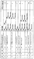
上記のマッピング行列は、一般的に疎行列であるように、スパース行列を格納するための通常の形式は、マトリックスおよび効率的な行列乗算演算を効率的に格納するために使用することができます。
ステップ6:
物理ネットワークのAAAでの転送(パス)の関係は現在、好ましくはすべて、にして、論理ネットワークVVVのすべての論理ノード間の可能な隣接関係を変換されています。
アポA すべて _ RPOA rPoATJPOA / R P°A \
VW - M VVV-AAA / KKK *(M AAA / KKK-AAA *ΓAAA * M AAA-AAA / KKK)「M <POA> AAA / KKK-VVVで後(M <POA> AAA / KKK-AAA * F <POA> AAA・M <POA> AAA-AAA / KKK)私は、jはiとインデックスjが同じノードを識別した場合の指数の値1(1)に設定されているセルの値。
ここで、好ましくは、完全な操作後のセルの値は、I、Jの値が0(ゼロ)に設定した場合の指数で指数iおよびjは、同一のノードを識別する。
計算の中間ステップは図28Kに示されている論理ネットワークUUUためにこのような行列A <PoAのすべて> UUUの例は、図28Lに示されています。
用語(M <POA> AAA / KKK-AAA・F <POA> AAA・M <POA> AAA-AAA / KKK)セルの値を持つI、値1(1)にj個のセットの場合のインデックスiおよびインデックス内jが同じノードは、すべての物理および仮想ノード間のパスを表して識別します。
行列A <PoAのすべて> VVV論理ネットワークVVVのすべての論理ノード間の可能な隣接関係が含まれています。それぞれのネットワークのAAAとKKKの物理および仮想ノード間のパスは、論理ネットワークVVVのすべての論理ノード間の可能な隣接関係に翻訳されていることに注意してください。対応するコスト型の隣接行列Aコスト型kのVVVはして算出された<すべてコストK>:
コストK すべて VW - iコスト K iコスト K Tjコスト K <■>iコスト K
M VVV-AAA / KKK *(M AAA / KKK-AAA * AAA * M AAA- AAA \ <■> iコスト K
/ KKKj * M AAA / KKK-VVV
これで後(M <コスト> ^ AAA / KKK-AAA・F <コストK> AAA・M <コスト> VA-AAA / KKK)の場合の指数のiは、jが0(ゼロ)の値に設定されているセルの値Iインデックスjが同じノードを識別します。
これでは、好ましくは、完全動作後のセルの値は、I、Jは、iおよびインデックスjが同じノードを識別する場合インデックスに(無限大)値∞に設定されています。
計算における中間ステップは図28Mに示されている論理ネットワークUUUためにこのような行列A <コスト1> <すべて> UUUの例は、図28Nに示されています。用語(M <コスト> VA / KKK-AAA・F <コストK> AAA・M <コスト> AAA / KKK)セルの値を持つ私は、値0(ゼロ)にj個のセットの場合のインデックスiおよびインデックスj内同じノードを識別することは、すべての物理および仮想ノード間のパスのコストを表します。
行列A <コストkはすべて> VWは、物理ネットワーク内のコストに基づいて、仮想マッピングおよび論理仮想/物理のコストへの物理的なコストを論理ネットワークVVVのすべての論理ノード間の可能な隣接関係の費用が含まれていますマッピング。
Aの計算<コストkはすべて> VVVはオプションです。
その値は、論理ネットワークVVVに隣接のコストを定義するために使用することができます。
なお、このステップ6は、2つのサブステップを実行するようにまとめることができることが観察されます。a)物理的な転送ポイントオブアタッチメントに応じて物理ノードと仮想ノードを含む、ノードのセット間のパスに物理ネットワーク内のパスを変換します関係と第一マッピング関係上、ならびにb)の物理ノードのセットと、仮想ノード間の経路上の第二に依存して論理ノード間の可能なリンク関係に物理ノードと仮想ノードのセット間のパスを変換しますマッピング関係。
ここでは、最初のマッピング関係は、仮想ノードと物理ノードが相互にどのようにマッピングされるかを定義し、第2のマッピング関係は、論理ノードが物理ノードと仮想ノードにマップする方法を定義します。
実際にこの最初のサブステップは、(M <POA> AAA / KKK-AAA * F <POA> AAA * M <POA> AAA-AAA / KKK)の計算を反映しており、第2のサブステップでは、計算の残りの部分を反映しています行列A <PoAのすべて> VWの。
ステップ7:
ステップ6から生じる可能性の隣接関係から、我々は論理ネットワークVVVの隣接関係を定義し、それぞれのコストタイプnの各隣接のコストをオプション。
値無限大のコスト(∞)は、2つのノード間の隣接関係がありません示しています。
論理ネットワークVVVのコストタイプとコスト値がコストタイプと物理ネットワークのAAA、仮想マッピングに物理のコストと論理マッピングに物理/仮想のコストのコスト値から完全に独立しています。
論理ネットワーク内のコストがに基づいて、論理ネットワーク内のコストが行列Aに格納されたコストに基づいて行うことができる行列F <コスト> ^ AAA-に格納されているが、物理ネットワーク内のコスト、と同じことができます<コストK すべて> VW。
ステップ8:
ステップ7で定義された隣接関係に基づいて、単一の隣接のPoA行列論理ネットワークVVVのA <PoAの> VVVが作成されます。
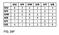
ネットワークUUUたとえば隣接行列A <PoAの> UUUを図29Bに示されています。一つ以上の添付隣接コストが作成され、<コスト> VVV、各コストタイプnの1行列します。
例えば隣接コストマトリックス
ネットワークUUUための<OS> UUUは、図29Aに示されています。
<PoAの> VVVに係るA <PoAのすべて> Vwの由来であります:
<PoAの> WV(i、j)は= 0の場合、A <原価N> WV(i、j)を等しいです∞(無限大)
<コストのN>ウエストバージニア(I、J)は(無限大)同じ∞ていない場合は、<のPoA> WV(i、j)が<PoAのすべて> VVV(i、j)を=
値無限大のコスト(∞)は、2つのノード間の隣接関係にかかわらず、使用される特定のコストタイプの、ありません示しています。
したがって、任意のコストタイプのは、<のPoA> VVV(i、j)を決定するために、上記の文で使用することができます。
場合には、<なPoA> VVV(i、j)の値は、SDNコンパイラのユーザによって定義された隣接関係を表す、1(1)に等しく、A <PoAのすべて> VVV(i、j)が、一連のではありませんPoAは、SDNコンパイラのユーザが指定した隣接関係が作成できないことを示す、エラーメッセージで通知されます。
ステップ9:私たちは、ネットワークVVV、ネットワークVVVで転送パスのセットにネットワークVVVでの隣接関係の翻訳を提供する基本的機能の転送ポリシーPvvvを定義します。転送ポリシーを適用する場合、論理ノードの特定のタイプ、図13に示すように、論理スイッチノードまたは論理ホストノードであることを考慮すべきです。
様々な転送ポリシーの例は、物理的なネットワークのための上記の手順4の説明に与えられました。
同じ例は、論理ネットワークの転送ポリシーに適用されます。
ステップ10:
論理ネットワークVVVの単一転送のPoA行列F <PoAの> WVが作成され、論理ネットワークVVV内のすべてのパスを含む、物理と仮想のPoAで表現。ネットワークUUUたとえば転送行列F <PoAの> UUUを図29Cに示されています。
一つ以上の添付の転送コストの行列Fに作成されているWV <コスト>」、各コストタイプnの1。
F <PoAの> VVVとF <コストN> VVVは、以下によって計算されます。
TJPはTjコスト N \ PoAのコストを°N \
(ΓVVV、ΓVVV) - 「WV(VVV、ウェストバージニア州)
ネットワークUUUのコスト行列F <コスト2> UUUを転送する例を図29Dに示されています。
適用されたポリシーPvvvに起因する任意の転送ループがiの要素を、転送行列のjの各列をスキャンして検出されたF <PoAの> VW重複入力ポートのため。
彼らはループ内で転送されるパケットをもたらすであろうとして転送ループがSDNコンパイラによって許可されていません。
ステップ11でSDNコンパイラによって作成された転送エントリの面では、それらは同一の論理ソース、論理宛先と物理または仮想入力ポートで複数の転送エントリをもたらすであろう。
転送ループが検出された場合には、次の可能なアクションまたは他の適切なアクションのいずれかまたは複数を撮影することができます: - 転送ループが重複入力ポート間でのPoAのシーケンスと同様に、最初に除去することにより、パスから削除されますこの重複した入力ポートの発生。
- 別のパスを指定し、代替ポリシーに基づいて計算されます
5 - SDNコンパイラのユーザに通知されます
これは、観察される転送行列F <なPoA> VVVとF <コストN> VVV(ステップ10の出力)が再帰を作成再びステップ5の開始点として使用することができます。
この場合、論理ネットワークは、ステップ5に行列F <のPoA> VVVは、F <コストn>はVVVのようになり、入力を転送する手順5から10に従うことによって、別の論理ネットワークSSSを作成することにより、表現します。
このvvv- <PoAの>その場合の10 MAAA / KKK-AAAとMAAA-AAA / KKKは、手順5で作成し、手順6で使用される行列は、転送行列Fの大きさと同じ大きさの両方のアイデンティティ行列の私であることになるのでご注意くださいステップ6の変換ステップを削減します:
すべてのPoA _ A、ΓΡΟΑTJPOAΛ,,ΡΟΑ
SSS - M SSS-VW *ΓVVV * M VW-SSS
そして、必要に応じて:
RコストのN すべて <■> iコスト Nコスト N Tjコスト N <■>
ポンドA SSS - M SSS-VW *ΓVVV * M VW-SSS
特定の論理ソースノードと、物理および仮想のPoAで発現される特定の論理宛先ノードとの間のすべての転送パスであること、「ネットワーク状態 'を含むWV行列F <PoAの>転送。ここでは、一般的にコンピューティングで使用される用語「状態」を使用しています。
行列F <PoAの> VVV転送すると、転送の動作を決定し
決定論的な方法で20物理および仮想ノード。
また、転送行列Fと<のPoA> VVVが行列を転送し、「ネットワーク状態 'を含むF <PoAの> VVVさらなる分析のためのいずれかSDNコンパイラまたはSDNコンパイラの外で使用することができます。
例として、転送行列F <POAは> VVVは、論理ノード名で識別される物理および仮想ノードによって報告された(例えば、トレースルート情報)をパストレースと照合することができ
25一貫性を確認します。
また、転送行列Fに含まれる「ネットワーク状態 '<のPoA> VVVはときに特定の「ネットワーク状態」を復元するために、(例えば、行列F <PoAの> VVVまたは定期的な間隔での転送の各変化の後に)特定の瞬間に保存することができました必要としていました。
ステップ11:
対応する転送テーブルエントリを計算できるようにするために、
VWは行列F <0> VVVとFをフォワーディング <OSTのn> で30 間の分離ホストとホスト
-開始:以下のプロセスに従って除去
ステップ1:ネットワークUUUたとえばwv-転送行列テーブルF Fと同じ<PoAの表> VWを<PoAの>作成マトリックス表を転送するF <PoAの表> UUUを図29Eに示されています。
ステップ2:ネットワークUUUの転送コスト・マトリックス表を作成したp Pコストに<コストのN表> vw同一の <n>はVVV ^ n個例フォワーディングコスト・マトリックス表F <コスト2表> UUUは、図29Fに示されています。
ステップ3:転送行列テーブルF <PoAのテーブル>内の各列のVWと転送:転送行列テーブルF <PoAの表> VWとF <コストN> <表> VWホストのノードステップ4によってインデックス付けの各行を削除しますコスト・マトリックス表F <コストN表> VWホストのノードによってインデックス付け、ホストによってインデックス付けた行を除いて、すべての行のホストノードに対応することにより、索引列に行列要素の値をコピーします。
ステップ5:転送行列テーブルホストのノードによってインデックス付けF <PoAの表> VWと転送コスト・マトリックス表F <コストのN表> VWの各列を削除します
-終わり
ホストノードは、現在のマトリックステーブルを転送行列内の単一ノードによって識別されます
FPOA表vwは^ ^ CQst行列taWepコスト n個表を転送します
転送行列テーブルF <PoAの表>の各出力ポートのためのVWの出力ポートは、次の項目で、誰に属する物理 または仮想ノードの転送エントリを作成します。
- 論理ソースノード:出力ポートが発生し、転送行列テーブルpPoA表^^・ηの要素の行インデックスi
- 論理宛先ノード:出力ポートが発生した転送マトリックス表pPoA表^^・ηの要素の列インデックスj - 入力ポート:入力ポートを位置(H-1)の出力ポートの位置hでのPoAの順序で、またはケースの出力ポートの「ローカル」とは、のPoAのシーケンスの最初のPoAです。
- オプションのロードバランシング識別子
- 出力ポート:各入力ポートの出力ポートフォワーディングマトリックス表F <PoAのテーブル>内のPoAのシーケンスの最後のPoAであるVW、以下の項目で入力ポートが属する誰に物理または仮想ノードの転送エントリを作成します:
- 論理ソースノード:フォワーディングマトリックス表の要素の行インデックスi
Fは、<表のPoA> VWれる入力ポートが発生
- 論理宛先ノード:入力ポートが発生した転送マトリックス表pPoA表^^・ηの要素の列インデックスj
- 入力ポート:入力ポート
- オプションのロードバランシング識別子 - 出力ポート: "ローカル"
「ローカル」入力ポート値で転送エントリは、パケットがそのノードによって送信されるべきであるため、ソース・ノードを表します。
「ローカル」出力ポート値で転送エントリは、したがって、パケットは、そのノードによって受信されるべき、宛先ノードを表します。
オプションの負荷分散の識別子は、複数のパスが論理ソースとネットワークVVVで論理宛先ノードとの間に存在する場合にも使用することができます。ケースでは複数のパスは、各パスを表すのPoAの特定の配列を含む、複数の行が含まれているWV論理ソースと論理宛先ノードの転送行列F <PoAの>の対応する要素の間に存在します。
例として、ロードバランサの識別子は、要素の値はそのパスに関連付けられた特定のロードバランシング識別子であると、行列F <PoAの> WVを転送すると同じ寸法とインデックスと負荷分散行列に記憶することができます。
マトリックス表pPoA表^^ ^この行列で間の分離ホストとホスト」を転送するための上記の方法と同様に、転送マトリクステーブルと同じ次元の負荷分散行列を作成するために除去することができます
FPOA表
VVV-同様に、SDNコンパイラは、現在使用中のパスが使用できない場合に使用することができる予備パス(複数可)を含有するマトリックスを維持することができます。
これは、図25のプロセス(一部の)の再計算を避け、サービスの迅速な復旧を可能にします。
バックアップパスの有用性は明らかに使用できない現在使用中のパスになります正確な原因によって異なります。
バックアップパス(複数可)は下記のように使用される新しいパスは、プロセスの再計算からもたらされる場合には、同様に使用できないかもしれません。
また、アプリケーションのポート識別子に限定上位などの識別子ではなく、は、転送行列F内の複数の可能な経路からの特定の経路を選択するために使用することができる<M> WV特定するための論理ソースノードと論理的な宛先ノードとの間のアプリケーションポート。
これは、特定のパスに沿って、特定のアプリケーションのトラフィックを転送することができます。
一例として、TCPとUDPポート番号は、アプリケーションのポート識別子として使用することができます。
F <PoAの表> VWとF <コストのNテーブル> VWを作成し、F <PoAの表> VWから転送テーブルエントリを計算するために、上記のプロセスの代わりに、転送テーブルのエントリも<のPoA> Fから直接計算することができますVVVは、プロセスは、上記と使用: - 場合には列がホストの代わりに、ホストの転送エントリに対応するホスト名を使用する 'でインデックスされま す
- によってインデックス付けセルを無視する(ホスト、ホスト')
行はホストによってインデックスされるようホストによってインデックス付けと列 'とホストによって索引付けされた列は、POAを含んでいない、何の反復がホストによってインデックスを付けた行の上に必要とされません」。
このアプローチは、Fを用いて、上記のアプローチと機能的に同等であることに注意してください<のPoA>
表
vvv-ステップ12:
転送テーブルのエントリは、現在「SDNコントローラのそれぞれのネットワークAAAおよび/またはKKの物理および仮想ノードへの転送テーブルエントリの配布を担当するに送信されます。
また、実装に応じて、「SDNコンパイラ」は、ネットワークAAAおよび/またはネットワークKKKの仮想ノードの物理ノードに直接転送エントリを送信することができます。
転送テーブルエントリは、物理または仮想ノードによって直接使用することができ、物理的または仮想ノードによる翻訳を必要としないと述べたノート。
繰り返しプロセス:
上述のようなプロセスは、全体であってもよく、または部分的に、任意の変更のような、任意の、物理的、仮想又は論理ネットワークまたはマッピングで行われるときに繰り返すことができる: - 物理ノード、物理ノードタイプ(スイッチノードは、ホストノード、NICノード)、物理ネットワーク、物理リンク、物理的なPoA、物理的なリンクコストの種類、物理的なリンクコストの値、物理的転送ポリシー
- 仮想ノード、仮想ノードタイプ(スイッチ・ノード、ホストノード)、仮想ネットワーク、仮想のPoA
- 論理ノード、論理ノードタイプ(スイッチ・ノード、ホストノード)、論理ネットワーク、論理リンク、論理リンクコストタイプ、論理リンクコスト値、論理フォワーディングポリシー
- 物理および仮想ノード間のマッピング、物理/仮想および論理ノードとの間のマッピング
スイッチ、ホストおよびNIC:図25の上記のフローチャートでは、ノードの様々なタイプの区別をしました。我々は、適切な転送ポリシーを適用できるようにするために使用するマトリックス中のNIC型とホスト型ノードを導入しました(例:
物理ネットワークと論理ネットワークにおけるSPF)。
代わりに、我々は、ノードの様々なタイプの区別をしないように選択し、使用するマトリックス中のNICの型とホスト型ノードを導入しませんでした。
図25のフローチャートで説明したのと同じプロセスを適用することができるが、追加の情報(ステップ4とステップ10で)転送ポリシーを適用する際に、特定のノードタイプの識別を追加しなければならない:スイッチ、ホストまたはNICを。私たちは別の方法として、図21 Aに指定された形式のPoAの型行列を使用した図25の上記のフローチャートでは、(括弧の間に示されている)「入力ポート」はPoAの型マトリックス中に省略することができました。
図25のフローチャートのステップ11の間、適切な物理的または仮想の「入力ポート」のPoAの配列またはその代わりに、転送テーブルエントリの各物理または仮想出力ポートの後に追加することができます。
特定の物理出力ポートに対応する物理入力ポートの値は、適切な物理PoA-タイプ隣接行列から得ることができます。
特定の仮想出力ポートに対応する仮想入力ポートの値は、仮想マッピングに対応する物理を表す適切なPoA型マッピング行列から得ることができます。
数学的に等価である、定義された行列の行と列を入れ替えることができることに留意されたいです。
図25のフローチャートで説明したプロセスは、図26の図に要約されています。
プロセスは、物理ネットワークのAAAのポリシーPを転送することは物理的なAAAの転送行列(POA型とコスト型)、その結果、塗布された物理ネットワークのAAAの隣接行列(POA型とコスト型)、で始まります。仮想マッピングに物理を記述する4のPoA型マッピング行列を使用し、論理ネットワークVVVの論理マッピングに物理/仮想隣接行列は、可能な隣接関係(図には示していない)を含む作成されます。
必要に応じて、仮想マッピングに物理的および論理的なマッピング、仮想/物理的なコストを記述する4費用型マッピング行列は、ネットワークVVVの可能な隣接のコストタイプkのコスト値を計算することができます。論理ネットワークVVVのために定義された隣接関係に基づいて、論理ネットワークVVVの隣接行列(POA型とコスト型)が作成されます。
論理ネットワークVVVの政策Pvvvを転送すると、論理ネットワークVVVの転送行列(POA型とコスト型)、その結果、VVVのこれらの隣接行列に適用されます。論理ネットワークVVVのPoAの型の転送行列が論理ネットワークVVV内のすべての論理ノード間のすべてのパスが含まれ、物理および仮想のPoAで表現、物理ネットワークのAAAと仮想ネットワークのすべての物理および仮想ノード用のフォワーディングテーブルKKが導出されます。
行列MAAA、MKKK、MVvvは、ノードと、それぞれの物理的なネットワークのAAA、仮想ネットワークKKKと論理ネットワークVVVのネットワーク間の関係を定義します。
図25に示した上記のプロセスでは、SDNコンパイラの典型的には、ユーザは、(入力)以下の項目を定義します。
論理ネットワークの1名
論理ネットワークを構成している論理ノードの2名
論理ノード間の3隣接関係
論理ネットワークの4つまたはそれ以上のコストタイプ
各コストタイプのための論理ノード間の論理的な隣接関係の5コスト
論理ネットワークの6転送ポリシー
論理ノードおよびオプションの物理的および/または仮想ノードから7のマッピング
マッピングコスト値
以下の項目は、通常、指定されたおよび/またはSDNコントローラ、サーバ管理システムやクラウド管理システム、またはこれらの組み合わせによって報告される:1。
仮想ノードの名前(リソース)
仮想ネットワークの2名(仮想ノードのコレクション)
3.仮想ノードタイプ(スイッチ・ノードは、ホストノード)
4.仮想のPoA
仮想ノードおよびオプションのマッピングコスト値への物理ノードから5のマッピング
仮想ノードによって実行される6.オプション機能(複数可)
以下の項目は、通常、指定されたおよび/またはSDNコントローラまたはネットワーク管理システム、サーバ管理システム、またはこれらの組み合わせによって報告されます。
物理ネットワークの1名
物理的なネットワークが構成している物理ノードの2名(リソース)
3.物理ノードタイプ(スイッチ・ノード、ホストノードは、NICのノード)
4.物理のPoA
物理ノード間の隣接関係5.
物理ネットワークの6つまたはそれ以上のコストタイプ
各コストタイプのための物理ノード間の物理的な隣接関係の7コスト
物理ネットワークF O 8.転送経口licy
物理ノードによって実行される9.オプション機能(複数可)
今では、我々は、ネットワークソフトウェア定義のための私たちの目標に達しています。
論理ネットワークは現在、完全にSDNコンパイラのユーザによって、ソフトウェアで定義することができ、これらのリソースのための命令で、その結果、任意の物理および仮想ネットワークとコンピューティングリソースに対してコンパイルすることができます。
複数の論理ネットワークが定義され、同一の物理的および/または仮想ネットワークおよび/またはコンピューティングリソースを同時に作成することができます。
また、私たちの方法は、ネットワーキングとコンピューティングリソースの両方のための説明書を作成、タイトとの統合および仮想ネットワークとコンピューティングリソースを制御します。
これは、物理スイッチノードの転送テーブルの通常の創造を超えて、物理ホストノード、物理NICのノード、仮想スイッチノードおよび仮想ホストノードに転送テーブルの作成を拡張します。
また、SDNコンパイラは、SDNを要求することができます
コントローラー、サーバ管理システムおよび/またはクラウド管理システムは、作成、変更、削除、および/または(別の物理リソースに)これはSDNコンパイラのユーザの要件を満たすために必要な場合に、仮想リソースを移動します。
また、SDNコンパイラは、変更することができる物理的なネットワークのプロパティを変更するには、例えば、SDNコントローラまたはネットワーク管理システムを要求することができます要求は、パケット交換網のノードを相互接続するために使用された場合に、リモート光アド/ドロップマルチプレクサ(ROADMs)または光クロスコネクトからなる光ネットワークの物理ノード間のリンクを変更します。
このように、SDNコンパイラは、例えばとしてSDNコンパイラの利用者のニーズに基づいて、物理および仮想ネットワークとコンピューティングリソースを最適化することができる中心的な構成要素(複数可)となりますアプリケーション。
ネットワーク内のパスは、さまざまな方法でインスタンス化することができます。
・プロアクティブパスのインスタンス - SDNコンパイラは(限り転送ポリシーは、これらのパスを可能にするように)ネットワーク内のすべての論理ソースと論理宛先ノード間の先行転送パスを 計算し、物理的および/または仮想ノードにすべての結果転送エントリを配布SDNコントローラを介して、または直接のいずれか。
・リアクティブパスのインスタンス化 - パケットが物理的に受信されると、又は
転送エントリに対して一致しない仮想ノードは、要求は、関連する転送エントリを提供するために、SDNコンパイラへの物理または仮想ノードによって行われます。
・ハイブリッド・パスのインスタンス化 - プロアクティブなパスのインスタンスと異なるパスのための反応パスのインスタンスの組み合わせ。
説明SDNコンパイラ方法は、パスのインスタンスのすべての3つの上記の方法をサポートするように構成することができます。
一例として、典型的な実装では、イーサネットMACアドレスは、物理および仮想のPoAを識別するためのPoA識別子として使用することができます。イーサネットMACアドレスは、グローバルに一意である多数のアドレスを提供するのに十分な長さ(48ビット)を有し、物理および仮想の両方のPoAを識別するために使用され、普及しています。
我々の手法では、ネットワークと論理名を持つノードの両方に名前を付けています。
一例として、典型的な実装では、IPv4アドレスのサブネットの一部は、論理ネットワークを識別するために使用することができ、IPv4アドレスのホスト部分には、論理ノードを識別するために使用することができます。
インタフェース識別子は、論理ノードを識別するために使用することができるが、一例として、代替的に、IPv6アドレスのグローバルルーティングプレフィックス+サブネット識別子は、論理的なネットワークを識別するために使用することができます。
現在のネットワークでは、IPv4とIPv6のアドレスは、インターフェイスではないノードを表しています。
これは、マルチホーミング問題などのIPネットワーキングではよく知られている制限を作成しています。
A)ノードを示すためにIPアドレスを使用する:これは、2つの方法で対処することができます。
ネットワークソフトウェア定義のようなインタフェースを示すために、IPアドレスが削除された期待の制御プロトコル上のノードの依存関係との間の制御プロトコルを必要としません。
b)の場合には、これは、可能ではない1:N論理マッピングに対する仮想/物理的には単一の物理的または仮想ノードのために複数の論理ノードを作成するために使用することができます。
各論理ノードは、単一の物理的または仮想ノードのための複数のIP-アドレス、その結果、IPアドレスが与えられます。
私たちは今、論理ノードとネットワークの命名を検討してください。
ネットワーク・オブ・ネットワーク・オブ・ネットワーク:提案されたアプローチをスケーラブルにするために、我々は次の形式のネットワークとノードの論理的な命名で階層をご紹介します。
ネットワーク・オブ・ネットワーク。
ネットワーク。
節点
ドット記号「。」論理名で構成されて異なる要素を分離します。
我々はNoNoNsとして、またNoNsなどのネットワーク・オブ・ネットワークへのネットワーク・オブ・ネットワーク・オブ・ネットワークを指します。上記の命名構造は、再帰的な方法で階層が導入されています。
ネットワークノードの集合です
NoNsはネットワークの集まりです
- NoNoNsがNoNsのコレクションです
そのために、使用される命名形態の上記の定義で示されているように。
これは明らかに実用的な制約に限定展開で、ネットワーク内の階層レベルの任意の数を作成します。
ネットワーク・オブ・ネットワーク・オブ・ネットワーク:ノードが配置されていることにより、上記の構造を採用しています。
ネットワーク・オブ・ネットワーク。
ネットワーク。
ネットワーク・オブ・ネットワーク・オブ・ネットワーク:ノードは、同様に、ネットワークが位置しています。
ネットワーク・オブ・ネットワーク。
ネットワーク
ネットワーク・オブ・ネットワーク・オブ・ネットワーク:同様に、NoNsが位置しています。
ネットワーク・オブ・ネットワーク
ように、階層内の様々なレベルのために。
これは、階層型ネットワーク内で、それのアドレスを介して、ノードを検索するための手段を提供します。
さらに、上記のアプローチは、ネーミング階層内の特定のレベルのノードにすべてのネットワークを抽象化します。
例えば
NoNsは、ネットワークノード間の隣接関係を持つノードの集合から成るさと同様に、ネットワーク間の隣接関係とネットワークの集合からなりますさ。
ドメイン間のノード(のIDN)の各種ネットワーク、NoNs年代、NoNoNs年代などの間で相互接続を提供
命名構造の階層に続いて、我々は、IDNを、次のタイプを区別することができます:
ネットワーク間でのIDN:隣接/隣接関係のIDNのペアの間には、2のネットワークの境界を横切ります。
- NoNs年代の間のIDN:隣接/ IDNドメインのペアの間の隣接関係
2 NoNsの境界を横切ります
NoNoNs年代の間のIDN:IDNドメインのペア間の隣接/隣接関係は、2 NoNoNsの境界を横切ります
ように、階層内の様々なレベルのために。
今、私たちは、IDNをからなるネットワークにSDNコンパイラの方法を適用し、IDNをからなるネットワークに、図25のフローチャートの処理を適用することができます。得られた転送テーブルのエントリは、IDNドメイン間の転送を示しています。 IDNドメインからなるネットワークのPoA-型フォワーディングマトリックスはまた、IDNが存在する内のネットワーク内の1つまたは複数のノードの転送動作が含まれています。
転送テーブルのエントリはのIDNが提供する階層レベルに応じなどのネットワーク、NoNs、NoNoNs、間の相互接続のために作成することができます。このように
以下のための相互接続。
IDNドメインがために相互接続性を提供するネットワーク階層レベルに応じてネットワークなど、NoNs、NoNoNs、間の転送パス(複数可)を決定し、IDNドメインポリシーのネットワーク内で適用することができることに注意してください。
宛先ノードへの宛先ネットワーク内のIDNから宛先ネットワークCにIDNに元ネットワークにIDNから)ソースネットワークBのIDNにソースノードからa)の転送転送)転送:転送がに分解されるNoNsため、上記の方法を使用して
転送テーブルエントリ)は、ソース・ノードのネットワークのPoA型転送行列から導出されます。
Cの転送テーブルエントリ)が宛先ノードのネットワークのPoA型転送行列から導出されます。
Bの転送エントリ)がIDNドメインのネットワークののPoA型転送行列から導出されます。
同じプロセスが再帰的に、階層の各レベルのために繰り返すことができます。
上記のアプローチは、間にNoNs年代、IDNの間でのIDNに拡張することができます
NoNoNs年代など
ネットワークのサイズは、ノードの非常に大きな数に拡張できる一方で、上記の再帰的な命名構造、隣接関係を使用することにより、転送とマッピング行列が上記で説明行列の高速計算を可能にする、合理的な大きさに保つことができることに注意してください。
また、転送テーブルのサイズは、IDNドメインのネットワークの転送ポリシーによって決定IDNドメイン間のパスの限られたセットを介してネットワーク間のノードのコレクションのトラフィックを転送することにより、合理的な範囲内に維持することができます。
一例として、上述したが、これらに限定されないように、単一の論理ネットワークからなる典型的な実施例では、IPv4アドレスのサブネットの一部は、論理ネットワークを識別するために使用することができ、IPv4アドレスのホスト部分を使用することができます論理ノードを識別する。
論理的な命名階層例として、ネットワークの階層をサポートするために、上記の、しかしこれらに限定されず使用する場合、ネットワークが、IPv4アドレスのホスト部分には、論理ノードを識別するために使用することができ、NoNs、NoNoNsなどでしIPv4アドレスのサブネットのクラスレスドメイン間ルーティング(CIDR)表記で表します。
IPv6は、インタフェース識別子を使用することができるが、グローバルルーティングプレフィックス+サブネット識別子は、論理的なネットワークを識別するために使用することができるアドレスの例として、上述したが、これらに限定されない、単一の論理ネットワークからなる典型的な実施例のように論理ノードを識別します。
ネットワークの階層をサポートするために、上記の論理的な命名階層を使用する場合、ネットワーク、NoNs、NoNoNsなどがIPv6グローバルルーティングのサブネットによって表すことができるが、IPv6アドレスのインタフェース識別子は、論理ノードを識別するために使用することができます接頭辞および/またはサブネット識別子アドレス。
SDNコンパイラによって制御されるネットワーク(複数可)内の論理ノードの移動性を支援するために、論理ノードはSDNコンパイラによって制御される、またはグローバルサポートするために、グローバルに一意であるされているネットワーク(複数可)内で一意の名前によって識別されるべきですモビリティ。
例として、限定されるものではないが、これは、二つ折り翼のいずれかの方法で実現することができる:a)は、IPv6アドレスのネットワークである部分に空間NoNs、NoNoNs等ノードBを表す部分を分割)ネットワークを示すために、ネットワーク、NoNs、NoNoNsなど、ノードを表すためにIPv4またはIPv6アドレスを導入するノードcを表す部分)及び第二のIPv4またはIPv6アドレスを表す部分にIPv4アドレス空間を分割、NoNs、NoNoNs。
単一の物理ネットワーク、単一の仮想ネットワークと、図25のフローチャートに示すように、単一の論理ネットワークのSDNコンパイラ方法は図面に示した例示的なネットワーク12、図13A、図13B、図14A、図14B、図15A-15Cに適用されます、16。
図27A-27E、28A〜28N、29A-29Fは、種々のマトリックスを表しており、図30A-30Iは、異なるノードDA-DG、およびHA、HBの転送テーブルを示している数字。
図12の物理ノードは、図13Aの機能モデルであり、図13Bの重み付き有向グラフに描かれています。我々は、物理ノードDA、DB、DC、DD、DE、DF、DG、DE '、DF'の集まりのような物理的なネットワークDAAを定義DG」の図の行列MDAA示しますに代表されるネットワークのDAA内の隣接関係がで表現されている27 A.行列A <POA> DAA(図27B)隣接関係のPOAを含有し、<コスト1> DAA(図27C)をマトリックス隣接関係のコストタイプ 'コスト1」のコスト値を含みます。
最短パスファーストフォワーディングポリシーPDAA使用してコスト型フォワーディングの「コスト1」の結果を適用すると、行列F <POA>のコスト値を含むパスと行列F <コスト1> DAA(図27E)のPOAを含むDAA(図27D)パスのコストタイプ 'コスト1」。
我々は、図28Aにネットワークマッピング行列MHAA示しますで表す仮想ノードHA、HBとHA」のコレクションとして仮想ネットワークHAAを定義します。図12および14(a)に示すように、仮想マシンのHAとHBの間のリンクがないよう、MHAAれていますにノードの単なる集まりにご注意ください。私たちは今、物理ネットワークDAAと仮想ネットワークHAAとの間で、最初のマッピングを定義します。 M <POA> DAA / HAA-DAA提供DAA(図28B) をネットワークへのネットワークDAAとHAA(DAA / HAAとして表される)からのマッピング、しばらくM <POA> DAA-DAA / HAA提供DAAをネットワークするためのネットワークDAAからマッピングとHAA(DAA / HAAとして表される)(図28C)。
物理ノードDAおよび仮想ノードHAとHBの間に2マッピング:図14Aおよび16を描い1で、このマッピングの破線。 M M <コスト1> DAA-DAA / HAAは、コストを提供しながら、<コスト1> DAA / HAA-DAAは、DAA(図28D)をネットワークにネットワークDAAとHAA(DAA / HAAとして表される)からのマッピングのコストを提供DAAとHAA(DAA HAAとして表される)(図28E)のネットワークへのネットワークDAAからのマッピング。
マッピングのコスト値は、この例では、物理ノードと仮想ノードの間のすべてのマッピングのためにゼロです。
論理ネットワークUUUは、図15のA(機能表現)に示し、15B(グラフ表現)を把握されています。
私たちは、図28Fに示すネットワーク・マッピング行列Muuuで表す論理ノードUU、UV、UW、UX、UY、UZ、UU '、UZ」のコレクションとして論理ネットワークUUUを定義します。現在、物理ネットワークDAA /仮想ネットワークHAAと論理ネットワークUUUの間、第2のマッピングを定義します。 M <PoAの> uuu- DAA / HAAはDAAとHAAをネットワークにネットワークUUUからのマッピングを提供
(DAA / HAA)(図28G)、M <POA> DAA / HAA-UUUは、UUU(図28H)をネットワークにネットワークDAAとHAA(DAA / HAA)からのマッピングを提供します。
M <コスト1> DAA / HAA-UUUネットワークDAAとHAA(DAA / HAA)からのマッピングのコストを提供しながら、DAAおよびHAA(DAA / HAA)(図281)をネットワークにネットワークUUUからマッピングのコストを提供UUU(図28J)をネットワークします。
マッピングコスト値は、この例では、すべての物理/仮想ノードと論理ノード間のすべてのマッピングのためのゼロです。
この例では1:によって示されるように、それぞれ使用されているノードDG、HB、DB、DC、DD、HA、DC、HA 'とUU、UV、UW、UX、UY、UZ、UU'、UZ 'の間の1のマッピング図15Cの点線。一般的な1:NまたはN:1マッピングを適用することもできます。
、物理、仮想、および論理ホストノードはホスト(送信ホスト)とホスト '(受信ホスト)のノードに分割されていることに注意してください。
物理または仮想ホストノードのノードが論理ホストにマップされている」一方で、物理または仮想ホストノードは、論理ホストノードにマップされます。
:物理ネットワークDAAで転送(パス)の関係は、今では論理ネットワークUUUのすべての論理ノード間の可能な隣接関係に変換されます
PoAのすべて _ RPOA rPoATJPOA / R P°A \
UUU <_> UUU-DAA / HAA *(M DAA / HAA-DAA *ΓDAA * M DA A-DA A / HのAA)「P <OA> DAA / HAA-UUU後(M <POA>でDAA / HAA-DAA * F <POA> DAA・M <POA> DAA-DAA / HAA)は、i、jが値1(1に設定されているセルの値)場合指標でiと指数jは、同じノードを識別します。
ここで、好ましくは、完全な操作後のセルの値は、I、Jの値が0(ゼロ)に設定した場合の指数で指数iおよびjは、同一のノードを識別する。
計算(M <POA> DAA / HAA-DAA・F <POA> DAA・M <POA> DAA-DAA / HAA)場合のセルの値を持つI、値1(1)にj個のセットにおける中間ステップインデックスiおよびインデックスjは、同じノードが図28Kに示されている識別します。 <PoAのすべて> UUUは、図28Lに示されており、論理的なネットワークUUUのすべての論理ノード間の可能な隣接関係が含まれています。
論理ネットワークUUUのすべての論理ノード間の可能な隣接関係のコストタイプ 'コスト1」のコストは次式で与えられます。
コスト1 すべて コスト1 コスト1 コスト1
UUU <_> UUU-DAA / HAA *(M DAA / HAA-DAA * DAA *
M コスト1 コスト1
DA A-DAA / HAA) 'M DAA / HAA-UUU
後(M <コスト1> DAA / HAA-DAA・F <コスト1> DAA・M <コスト1> DAA-DAA / HAA)は、セルの値をI、Jは、値0(ゼロ)に設定した場合の指数では、私はとインデックスjは、同じノードを識別します。
これでは、好ましくは、完全動作後のセルの値は、I、Jは、iおよびインデックスjが同じノードを識別する場合インデックスに(無限大)値∞に設定されています。
セルの値と計算(M DAA / HAA-DAA * F <コスト1> DAA * M <コスト1> DAA-DAA / HAA)における中間ステップ私は、値0(ゼロ)にj個のセットの場合指数のiとインデックスjは、同じノードが図28Mに示されている識別します。 <コスト1 すべて> UUUは、図28Nに示されており、論理的なネットワークUUUのすべての論理ノード間の可能な隣接関係のコストタイプ 'コスト1」の費用が含まれています。
図15Aに定義されたネットワークUUUの特定コストタイプのリンクおよびリンクコスト値によると、私たちは「コスト2」が(図29A)使用コストタイプであることと、<コスト2> UUUを作成15Bを把握。
値無限大(∞)のコストは、2つのノード間には隣接関係がありません示しています。
コストタイプ論理ネットワークUUUのコスト2、そのコスト値がコストタイプのコストl、そのコスト値から完全に独立しています。
しかし、一つはF <コスト1> DAAand /またはA <コスト1 すべて> UUU-で使用されたコスト値を使用するように選択することができます
論理ネットワークUUUの単一隣接のPoA行列A <ROA> UUUを図29(b)に示すように、<コスト2> UUUとA <PoAのすべて> UUUに基づいて作成されます。最短パスファーストフォワーディングポリシーPuuu使用してコストタイプ転送の「コスト2」の結果を適用すると、行列のコスト値を含むパスと行列F <コスト2> UUU(図29D)のPOAを含むF <PoAの>(図29C)パスのコストタイプ 'コスト2」。
対応する転送テーブルエントリを計算することができるようにするために、プロセスに応じて、<なPoA> UUUおよびF <費用> UUUが除去されたFでホストとホストとの間の分離は、「図25のフローチャートのステップ11で説 明しました。
その結果、ホストノードが今で識別のある行列内の1つのノードF <PoAの表> UUUとF <コスト2表> UUU図29Eは、それぞれ、図29Fに示されています。
得られた転送テーブルを、図30に示されています。
転送エントリUUU Fの各出力ポート<PoAの> <表>は、出力ポートが所属先である物理ノード(DA、DB、DC、DD、DE、DF、DG)または仮想ノード(HA、HB)のために作成されているため、以下の項目を持ちます。
- 論理ソースノード:Fの要素の行インデックスiの出力ポートが発生する<PoAの表> UUU
- 論理宛先ノード:Fの要素の列インデックスj出力ポートが発生する<PoAの表> UUU - 入力ポート:入力ポートを位置(H-1)の出力ポートの位置hでのPoAのシーケンスまたは「ローカル」にケースの出力ポートでのPoAのシーケンスの最初のPOAがあります。
- 出力ポート:出力ポート
入力ポートは、物理のために作成されている所属先である物理または仮想ノードの転送エントリUUU F <PoAのテーブル>内のPoAのシーケンスの最後のPoAで各入力ポート(ノードDA、DB、DC、DD、DEのため、以下の項目とDF、DG)または出力ポートが属している人に仮想ノード(HA、HB)、:
- 論理ソースノード:Fの要素の行インデックスi入力ポートが発生した<PoAの表> UUU - 論理宛先ノード:Fの要素の列インデックスj入力ポートが発生した<PoAの表> UUUを
- 入力ポート:入力ポート
- 出力ポート: "ローカル"
任意のロードバランシングの識別子は、この例では使用されません。
転送テーブルのエントリは、現在の実装に応じて、「SDNコントローラの責任を転送テーブルエントリの配布のためにまたは代替的に、直接の物理的および仮想ノードへと送信することができます。
任意の変更は、図25に示すプロセスの任意の、物理、仮想または論理ネットワークまたはマッピング(の一部)で起こるときに繰り返されます。
この例で使用される種々のマトリックスの等価物はまた、図26の図に示されています。
30A-30I物理および仮想ノードの図に示す転送テーブルは、特定のノードのノードタイプを反映:
- 物理的なスイッチは、DA、DB、DC、DDノード:論理ノードUW、UX、UY物理スイッチにマッピングされたが、DB、DC、DD、ノードDB、DCの、したがって転送テーブル、DDはソースでトラフィックの転送 エントリが含まれているノードまたはそれぞれの論理ノードの宛先。
DB、DCとして、DDは交通から生じるまたは他のノード宛に転送され、スイッチノードです。
(入力ポートまたは出力ポートの値を持つ無フォワーディングエントリ「ローカル」)トラフィックのみを起源または他のノード宛に転送されるため、何の論理ノードは、ノードのDAを切り替えるためにマッピングされなかったことに注意してください。
物理ホストノードDG:転送テーブルには、送信元または宛先ノードとして論理ノードUUを描いた唯一の転送エントリが含まれています。
目的の動作ごとのように、何の転送はホストノードDGで行われていません。
- 物理NICは、DE、DFノード:論理的ノードは、NICのノードにマッピングされていないことができ、したがって、NICはDE、DFが唯一の他のノードから発信されるパケットの転送を提供するノード。
それぞれのノードとノードDE、DFのポートP81とP82とポートP79とP80との間に固定された転送の関係に注意してください。
- 仮想スイッチノードHB:論理スイッチ・ノードのUVが仮想スイッチノードHBにマッピングされた、したがって、ノードHBの転送テーブルには、送信元または宛先UVをトラフィックの転送 エントリを含んでいます。 HBは、スイッチ・ノードのトラフィックから発信または他のノードのために運命づけられているように転送されます。
仮想ホストノードHA:転送テーブルは、送信元または宛先ノードと論理ノードUZを描いた唯一の転送エントリが含まれています。
目的の動作ごとのように、何の転送は、ホストノードのHAに場所を取りません。仮想スイッチ・ノードHBは、ネットワーク機能の可視化(NFV)を示しています。仮想マシンで実現される仮想スイッチノードは、トラフィックが転送され、それを通して物理ネットワークDAA、で導入されます。
典型的には、仮想スイッチ・ノードのような任意の操作を実行するが、1つまたはそれ以上にパケットを転送する前に、着信パケットのヘッダおよび/またはペイロードの監視および/または記録および/またはバッファリングおよび/または修正に限定されるものではないであろう出力ポートです。
仮想スイッチ・ノードHBは、(ブロック)パケットを転送しない場合があります。
アクションの最小セットと方法は、括弧間の参照は、図25に関連する上記のステップに加えられた(以下のように定義することができ、本発明に従ったSDNコンパイラによって実行される、しかし、ここで以上の文言定義などのアクション一般に)論理的ネットワークモデルに基づいて、コンパイラは、ネットワークを制御する方法、物理ノードと仮想ノードの第二の数の最初の番号を含むネットワークは、最初の数が1以上あることを特徴と、第二の数があることを特徴と等しいか、0より大きいが、第一および第二の数字は、それらの合計は、少なくとも2つの、物理的なネットワークレイアウトに従って、物理リンクによって相互接続された物理ノード、論理ノードの第3の数を含む論理的ネットワークモデルであるようにあることを特徴と、各論理ノードは、各論理ノード名は、次のアクションを備えたコンパイラを実行した場合と同様に、少なくとも1つの物理またはネットワーク内の少なくとも1つの仮想ノードは、この方法を参照して、論理ノード名で示されている:a)は、物理ノード名を保存します、各物理ノード名は、一意であること
一つの物理ノードの識別子、及び当該物理ノードのポイントオブアタッチメントの各名称は、ポイントオブアタッチメント懸念特定の物理ノードの間のユニークな識別子である、物理ノードを前記ポイントオブアタッチメントの名前を格納そして、物理ノードを接続する物理リンクは別の物理ノード[参照に関係しますステップ1と図25の2]; B)の物理パスを定義する物理的な転送ポイントオブアタッチメント関係を格納する物理的な転送ポリシーに依存して物理的なネットワークは、物理ネットワークは、物理ノード名が言った、とにした物理ノードのポイント・オブ・添 付ファイル名を言った上で、前記、物理的な宛先ノードに物理的なソースノードからのパケットは、以下の物理的な経路を示す物理パス[参照ステップ3と図25の4]; C)仮想ノードと前記物理ノードが相互にマップされ、論理ノードが物理ノードと仮想ノードにマッピングされる前記方法を規定する第2のマッピング関係を記憶していると述べた方法を規定する第1のマッピング関係を記憶し、仮想ノード名を格納する[CF 。図25のステップ5]; D)に依存して物理ノードと仮想ノードが物理的な転送ポイントオブアタッチメント関係述べたとの最初のマッピング関係を述べただけでなく、間にパスを変換すると述べた前記ノードのセット間のパスへの物理的なネットワークがセット前記内のパスを変換します依存して論理ノードが間にパスが物理ノードと仮想ノードのセットとの第2のマッピング関係を前記前記の間の可能なリンク関係に物理ノードと仮想ノード[参照図25のステップ6]。 ; E)は、前記論理ノードと論理ノードは、言っ間の論理的なリンクのセットのための論理ノード名を保存します[参照図25のステップ7]はF)で論理パスを定義する論理的な転送ポイントオブアタッチメント関係の計算の論理的な転送ポリシーに依存して論理ネットワークは、論理ノード名を言うと、上の論理リンクの前記セットに、論理ネットワークを前記しました言っ論理ノード、パケットは論理的な宛先ノードに論理ソースノードから次の論理的な経路を示す論理パス、[参照の間言った物理ノードの転送テーブルエントリを作成する手順8、9および図25の10] g)および仮想言っ
言っ論理転送ポイントオブアタッチメント関係からノード。 [参照図25のステップ11] H)選択された物理ノードと選択された仮想ノードに、直接または間接的に、言った転送テーブルのエントリを送信する、[参照図25のステップ12]
上記の明細書において、参照等コントローラ、コンパイラ、ノード、仮想マシン、NICのように、装置の多くの異なる種類に対して行われています
当業者には明らかなように、このようなユニットの機能は、処理装置上で実行しているハードウェアおよびソフトウェアのうちの少なくとも1つによって実行されます。
このようなハードウェアは、特許請求の範囲に記載の機能を実行するように構成されたハードウェア(現在および将来の)の任意の既知のタイプであってもよいです。
図31は、このような機能を実行することができるコンピュータ装置の概略図を示します。
図31は、「完全な」画像の種類を示しています。それは(プリンタなど)いくつかのコンポーネントは、現在のドキュメントで指定された単位の多くに使用されない可能性があることは明らかであろう。
図31に示す構成は、算術演算を実行するためのプロセッサ1を備えます。
プロセッサ1は、ハードディスク5、読み取り専用メモリ(ROM)7を含む、メモリコンポーネントの複数に接続され、電気的消去可能プログラマブル読み取り専用メモリ(EEPROM)10、およびランダムアクセスメモリ(RAM)11。
これらのメモリタイプのすべてを必ずしも設ける必要はありませ。
また、これらのメモリコンポーネントは、プロセッサ1に物理的に近接して配置される必要はないが、プロセッサ1から遠隔に配置することができます。
プロセッサ1はまた、キーボード13、及びマウス15のような、ユーザにより命令、データ等を入力するためのユニットに接続されています。
このような当業者に知られているタッチスクリーン、トラックボール及び/又は音声変換器等の他の入力装置は、あまりにも提供されてもよいです。
プロセッサ1に接続された読取ユニット17が設けられています。
読取部17は、データを読み取り、おそらくフロッピーディスク19またはCDROM 21のようなデータキャリア上にデータを書き込むように構成されています。
当業者に知られているように、他のデータキャリアは、テープ、等DVD、ブルーレイディスク、コンパクトフラッシュ(CF)、セキュアデジタル(SD)、マイクロSD、ミニSD、エクストリームデジタル(xDで)、およびメモリスティックであってもよいですアート。
データ記憶媒体は、プロセッサ1は、本発明による方法を実行できるように、プロセッサ1によって読み取られ、読み取られた後にされるように配置された命令及びデータを含むコンピュータプログラム製品を備えることができます。
このようなコンピュータプログラム製品は、メモリコンポーネント5、7、9、11のいずれかにロードされてもよいです。
しかしながら、そのようなコンピュータプログラム製品は、あるいは、通信ネットワーク27を介してダウンロードしてもよいです。
プロセッサ1は、例えば、ディスプレイ3と同様に、紙の上に、モニタまたはLCD(液晶ディスプレイ)スクリーン、プラズマディスプレイパネル、有機発光ダイオード(出力データを印刷するプリンタ23に接続されてもよいですOLED)、アクティブマトリックスOLED(AMOLED)または当業者に公知の他の任意のタイプのディスプレイ。
プロセッサ1は、通信ネットワーク27に接続することができる、例えば、パブリックIによって電話網(PSTN)などのローカルエリアネットワーク(LAN)、ワイドエリアネットワーク(WAN)、インターネット、スイッチ/ Oユニット25。
プロセッサ1は、ネットワーク27を介して他の通信の構成と通信するように構成されてもよいです。
プロセッサ1は、スタンドアローンシステムとして、または各々がより大きなコンピュータプログラムのサブタスクを実行するように構成された並列動作する複数のプロセッサとして実装、またはいくつかのサブプロセッサを有する1つ以上のメインプロセッサとしてすることができます。
本発明の機能性の部分であっても、ネットワーク27を介してプロセッサ1と通信するリモートプロセッサによって実行されてもよいです。
これまで我々は、単一の物理ネットワーク、単一の仮想ネットワークと単一の論理ネットワークのSDNコンパイラ方法を考えました。
上記のように、本発明は、適切な物理的および/または仮想ネットワークおよび/またはコンピューティングリソースのための命令のセットにハイレベルのネットワークの仕様を翻訳又はコンパイルするための方法を提供します。
a)組み合わせた物理的および仮想ネットワークは、1つまたは複数の層で構成されている:実行可能なこの方法に基づいて、大規模ネットワークの展開を行うために、我々は、以下の特性を有する任意のネットワークに本手法を拡張します。
各レイヤでは、ノードは、物理的および/または仮想リンクを介して相互接続することができます。
物理リンクは、以下を含むが、光ファイバケーブル、銅ケーブル、空気、これらに限定されない、任意の物理媒体とすることができます。
物理リンクもではなく、光波長、時分割多重(TDM)回路、マルチプロトコルラベルスイッチング(MPLS)パスに限定などの他のネットワーク技術、提供するパスすることができます。
物理リンクもGRE-トンネル[GRE =総称ルーティングカプセル化]、NVGRE -tunnel [総称ルーティングカプセル化を使用してNVGRE =ネットワーク仮想化]、VXLANトンネル[VXLAN =に限定などではなく、別のネットワーク技術により提供されるトンネルすることができます仮想拡張ローカルエリアネットワーク]。
仮想リンクは、仮想スイッチと仮想マシン間の仮想リンクを含むがこれらに限定されない仮想接続、仮想マシン、ネットワークソケットの間に仮想リンクすることができます。
B)層は、上位層にサービスを提供するかもしれないし、下位層からサービスを消費する可能性があります。 c)は、上記の層のそれぞれにおける物理的および/または仮想ノードは、パケット交換又は回線交換ノードのいずれかです。
例のパケット交換ノードがありますが、IPv4対応のルータ、IPv6対応のルータ、スイッチMPLS- [MPLS =マルチプロトコルラベルスイッチング]、パケット交換を提供するアプリケーション・プロセスに限定されるものではありません。
転送機能の他にスイッチにパケットを転送する前に、着信パケットのヘッダおよび/またはペイロードの監視および/または記録および/またはバッファリングおよび/または修正に限定されるようではなく、パケットに追加の操作(単数または複数)を提供するかもしれませんそれの出力ポートの一つ以上。
スイッチは、(ブロック)パケットを転送しない場合があります。
回線交換ノードの例としては、限定するものではないが、光ファイバ4クロスは、リモート光アド/ドロップ、相互接続する光ファイバを接続し
マルチプレクサ(ROADMs)や光クロスコネクトのクロス接続する光の波長を、同期デジタル・ハイアラーキ(SDH)マルチプレクサまたは
同期光ネットワーク(SONET)マルチプレクサは、時間スロットを相互接続します。
パケット交換ノードと回線交換ノードの両方のための命令セットは、SDNコンパイラによって作成されます。
パケット交換ノードの場合には、これらの命令は、転送テーブルのエントリを含みます。
circuit-スイッチングノードの場合には、これらの命令は、クロスコネクト設定を含みます。
d)の最低パケット交換層がする、メディアアクセス制御(MAC)e)の各層は、階層レベルの任意の数のサブネットワークの階層内のサブネットワークの任意の数で構成さを提供
F)論理ネットワークは、1つ以上の層で構成されています
G)論理層は、パケット交換または回線交換のいずれかにマッピングされます
物理、仮想および/または組み合わせた仮想/物理層
H)各論理層は階層レベルの任意の数のサブネットワークの階層内のサブネットワークの任意の数で構成されてい
私たちは次のように任意のネットワークをモデル化することによって、私たちの方法を拡張します。
- ネットワークがリンクによって相互接続ノードで構成されます。
成るネットワークのドメイン内でこれまでに説明した方法が適用されるノード。
- ネットワークは、ノードに抽象化することができ、他のネットワーク内のノードになることができます。
これは、図32Aおよび32Bに示されています。図32Aは、例えば、論理ネットワーク・オブ・ノードYVV、YWW、YXX、YYYからなる例論理ネットワーク・オブ・ネットワーク・オブ・ノードYYYYの機能を示します。論理ノードYA、YB、YC、YKから構成YVV論理ネットワーク・オブ・ノード。論理ネットワーク・オブ・ノードywwが論理ノードYD、YE、YFで構成されています。論理ネットワーク・オブ・ノードYXXは論理ノードYG、YH、YJで構成されています。論理ネットワーク・オブ・ノードYYYは、論理ノードYL、YM、YNで構成されています。図32Bは、どのように論理的なネットワーク・オブ・ノードYVVを示し、YWW、YXX、YYYは論理ノードに抽象化されます。
任意のあいまいさを避けるために、以下、我々はレベル(H-1)でネットワークから成るHレベルのネットワークに参照します。
これは物理的なネットワーク、仮想ネットワークと論理ネットワークに適用されます。
この用語を使用して、Hレベルの論理ネットワークYYYYは(H-1)レベルの論理ネットワークYVV、YWW、YXX、YYYで構成されています。
レベル(H-1)での論理ネットワークYVVは、論理ネットワークYA、YB、YC、YKレベル(H-2)で構成されています。
レベル(H-1)での論理ネットワークywwがレベル(H-2)での論理ネットワークYD、YE、YFで構成されています。
レベルの論理ネットワークYXX(H-1)は、論理ネットワークYG、YH、レベルのYJ(H-2)で構成されています。
レベル(H-1)での論理ネットワークYYYは、レベル(H-2)での論理ネットワークYL、YM、YNで構成されています。
私たちは、0(ゼロ)から始まる正の整数で時間を数えます。
ネットワークの階層内の最も低い時間とのネットワークは、これまでに言及「ノード」に等しいです。
- 全体的なネットワークは層で構成されています。
我々は、nが0(ゼロ)から始まる正の整数で、層nとして特定の層を参照してください。
私たちは、「最下層」としてn = 0のレイヤを参照してください。
現在のネットワークにおける層の例であるが、物理媒体層、周波数または波長分割多重層、時分割多重層、データリンク層、ネットワーク層、トランスポート層、アプリケーション層、これらに限定されません。
全体的なネットワーク層内のn層(N + 1)と層(N + 1)にサービスを提供するには、層nによって提供されるサービスを消費します。
- SDNコンパイラプロセスごととして論理ネットワークは物理ネットワーク、仮想ネットワークまたは組み合わせた仮想/物理ネットワークから作成することができ、これまでに説明しました。
上記のように、転送行列F <なPoA> VVVとF <コストN> VVV(図25のフローチャートのステップ10の出力)を出発点として使用することができる。また、論理ネットワークは、他の論理ネットワークから作成することができ再び図25のフローチャートのステップ5、再帰を作成します。
任意のあいまいさを避けるために、我々は以下の深さで、ネットワークから作成された深さd(D-1)でネットワークに参照します。
私たちは、dは0(ゼロ)から始まる正の整数で、深さdのような特定の深さを参照してください。
深さd = 0は、物理または仮想ネットワークに等しいが、これまでと呼ばれます。
深さD> = 1 がこれまでに言及論理ネットワークに等しいです。
上記は、図33A、33B、33Cに示されています。図33Aは、ネットワークKAとKBが同じレベルhであることと、リンクによって相互接続されているを示しています。
図33Aに示されるように、ネットワークKA及びKBネットワークは、他のネットワークと相互接続することができます。
ネットワーク間の関係をマッピングと呼ばれます。
今後導入されるであろう様々なマッピングの一貫性のあるネーミングを持つために、我々は、トポロジ・マッピングではなく、下のテキストのリンクのモデル化における隣接する参照します。
ケースでは、リンクは、リンクがネットワークの対の間のトポロジ - マッピングのペアを作成し、双方向です。
ケースでは、リンクは、リンクがネットワークのペア間の単一のトポロジ・マップを作成し、単方向です。
トポロジ・マッピングは、第一及び第二のネットワークは、同じ深さdと同じ層nである、第1ネットワークから第2ネットワークへのマッピングです。
図33Bは、ネットワークKA、KB、KC、KDは、同じレベルの時間であることを示しています。
ネットワークKAとKBがトポロジーマッピングとして表さリンクによって相互接続されています。
ネットワークKAおよびKCは、レイヤマッピングとして表さリンクによって相互接続されています。
ネットワークKBおよびKCは、レイヤマッピングとして表さリンクによって相互接続されています。
レイヤマッピングは、第一及び第二のネットワークは、n個の異なる層である、第1ネットワークから第2ネットワークへのマッピングです。
図33C網KA、KB、KC、KD、LA、LB、LCでは、LDが示されています。
この図の中で、各ネットワークは、同じレベルの時間を持っています。
階層レベルがH = 0で開始する場合には、図33CでH = 0でのネットワークは、「ノード」に等しいこれまで、場合には図33CにおけるH =ラ・ネットワークは、「ネットワーク・オブに等しいと呼ばれますノードなど、これまでに言及ネットワーク・オブ・ネットワーク・オブ・ノード ''これまでに、ケースH = 2で図33に、ネットワークがに等しいと呼ばれます "
各ネットワークは、特定の深さdと層nに位置します。
ネットワークKA及びKBは、深さdは、層nである場合、ネットワークKCおよびKDは、深さdは、層(N + 1)、ネットワークLA及びLBは深さである(D + 1)、層n、ネットワークLCとLDにあります深さ(D + 1)、層(N + 1)での。
私たちは、特定のレベルhでのネットワークとの間のマッピングの3種類を区別: - トポロジのマッピングは、同じ深さdと層nとネットワーク間の隣接関係です。
隣接関係がマッピングであることに注意してください。
私たちのイラストが3次元に制限されているとして、図33Cは、2ネットワーク(KA及びKB、KC、およびKD、LAとLB、LCおよびLD)の間の唯一のトポロジ・マッピングを示します。
一般に、トポロジ - マッピングは、ネットワークの任意の数の間に存在することができ、一般的に2次元レイアウトとして提示され、ここで提示SDNコンパイラ方式でサポートされています。
トポロジ・マッピングは、実線で示されています。
仮想マッピングへの物理的には、物理 および仮想ノード間のトポロジのマッピングの特殊なタイプです。
- レイヤマッピングは、異なる層のnと同じ深さdにおけるネットワーク間の関係があります。
レイヤマッピングは、ストライプ状に示されています。
- 深度マッピングが異なる深さdのネットワーク間の関係があります。
論理マッピングに物理的または論理的なマッピングの仮想は、これまでの深さのマッピングの例ですと呼びます。
深度マッピングは破線で示されています。
今後我々は、深さd = 0でネットワークに層n、レベル= 0時間ではなく、物理または仮想ノードを参照します。
今後、我々は深さd> =リットル、層n、レベルh = 0ではなく、論理ノードのネットワークに参照します。
ネットワークKAとネットワークLDとの間に図33Cの深さ・マッピングでは、ネットワークKBとネットワークLCの間で、ネットワークKCとネットワークLBとの間で、ネットワークKDとネットワークとの間で、LAは、比較的単純な図形を維持することが示されていません。
図33Cのトポロジ - では、層 - と深さのマッピングは、単一のネットワークKA、KB、KC、KD、LA、LB、LCまたはLDに接続されており、オープンエンド」であることが示されています。 。 。もう一方の側に '。
これらの層のマッピングは、レイヤマッピングは、層の任意の数に拡張することができることを示します。
単一のネットワークに接続された深さマッピングは奥行きマッピングは深さの任意の数に拡張することができることを示します。
後述するようにレベル(H + 1)レベル時間描いトポロジ・マッピングで単一のネットワークに接続されているトポロジ - マッピング。
異なるレベルのネットワーク間で、我々はレベルのマッピングを考えて:
- レベルのマッピングが異なったレベルと同じ深さDと同じ層nのネットワーク間の関係です。
レベルのマッピングの例は、Hレベルのネットワークからなるレベルでネットワーク(H + 1)です。
レベルマッピングマトリックスの例は、図28Fに示すネットワークマッピング行列です。
レベル・マッピングは、図34Aに示されています。図34Aは、HレベルのネットワークKA、KB、KC、KD、LA、LB、LC、LDとそのトポロジーマッピング、レイヤマッピングおよび深さ優先のマッピング関係を示しています。
図33Cに示されたノードKAおよびKD、KB及びKC、LAとLD、LBとLC間の対角層のマッピングは、図を簡単にするために、この図では省略されています。
図33Cに示されたノードKAとLA、KBとLA、KCとLD、KDおよびLC、KAおよびLC、KCとLA、KBとLD、KDとLBとの間に斜めの深さのマッピングは、この図では省略されています図を簡略化します。
図34Aはまた、ネットワークKAA、KCC、LAA、LCCレベルでの(H + 1)を示しています。
(D、N、H + L)でネットワークKAAは(D、N、H)でネットワークKA及びKBの両 方が含まれている、つまりネットワークにKAAは、ネットワークKAとKBにレベルマッピングによってマッピングされています。 (D、N + L、H + L)でネットワークKCCは(D、N + L、H)でネットワークKCとKDの両方が含まれている、つまりネットワーク内のKCCはネットワークKCとKDにレベルマッピングによってマッピングされています。 (D + L、N、H + 1)のネットワークLAAは、(D + L、N、H)でネットワークLAおよびLBの両方が含まれ、すなわちネットワークLAAはネットワークLA及びLBにレベルマッピングを介してマッピングされています(D + L、N + L、H + L)のネットワークLCCは、両方の(d + L、N + L、H)にネットワークLC及びLDを含んでいる、つまりネットワークにLCCはネットワークLCにレベルマッピングを介してマッピングされていますLD。
することができる第1ネットワークから第2ネットワークへ、レイヤマッピング、深さ優先マッピングまたはレベルマッピング(仮想マッピング物理含む)トポロジーマッピング1:1,1:N、またはN:Lマッピング(第一のネットワーク。第二のネットワーク)。
私たちは今、図34Aと同様の図ではネットワークKAA、KCC、LAA、LCCを表すことができます。図34Bは、図34Aと同様にネットワークKNN、KPP、LNN、LPPとそれらのマッピング関係に示されたネットワークKAA、KCC、LAA、LCCを示しています。
対角層 - マッピングおよび斜め深さのマッピングは、図を簡単にするために、この図では省略されています。
この図内の各ネットワークは、同じレベル(H + 1)を有しています。
基準に図34AにHレベルの単一のネットワークに接続されたトポロジマッピングは、図34Bに31、32、33、34、トポロジマッピングのレベルを示している(H + 1)で、33 32、31によって参照されます、34。
図35のAにおいて、我々は、単一の物理ネットワーク、単一の仮想ネットワークと、我々がこれまで検討している単一の論理ネットワークのSDNコンパイラ方法を示します。
図35Aは、ネットワークKE、KF、KG、KH、LE、LFとのマッピング関係を示しています。
我々は唯一のこれまでノードのネットワークを検討しているように、すべてのネットワークは、レベルh = 0です。
深さd = 0、層n = 0で、レベルh = 0でネットワークKE及びKFは、これまでの物理ノードと呼ばれました。
深さd = 0、層のn = 0、レベルh = 0でのネットワークKGとKHは、これまでのように仮想ノードと呼ばれていました。
深さd =リットル、層のn = 0、レベルh = 0でのネットワークLEとLFが、これまでのように論理ノードと呼ばれていました。
ネットワークKEとネットワークKFとのトポロジー・マッピングは、これまでの物理リンクと呼ばれていました。
ネットワークLEとネットワークLF間のトポロジ・マッピングは、これまでの論理リンクと呼ばれていました。
ネットワークKGとネットワークKHの間には、トポロジ・マッピングは、直接仮想ノードとしてモデル化仮想マシンとの間のリンクがないとして、これまで考えられませんでした。
仮想ノード間のトポロジのマッピングがあるしかしある状況が存在する場合があります。
ネットワークKEとネットワークKG間のトポロジ・マッピングは、仮想マッピングへの物理と呼ばれていました。
ネットワークKFとネットワークKH間のトポロジ・マッピングは、仮想マッピングへの物理と呼ばれていました。
ネットワークKEとネットワークLE間の深さ、マッピングは論理マッピングに物理と呼ばれていました。
ネットワークKFとネットワークLF間の深さ、マッピングは論理マッピングに物理と呼ばれていました。
ネットワークKGとネットワークLE間の深さ、マッピングは論理マッピングに仮想と呼ばれていました。
ネットワークKHとネットワークLF間の深さ、マッピングは論理マッピングに仮想と呼ばれていました。
図35Bは、レベルh = 1 とそれらのマッピング関係でネットワークKEE、KGG、LEEを示しています。
深さd = 0、層n = 0で、レベルh = 1 のネットワークKEEは、これまでのような物理的なネットワークと呼ばれました。
ネットワーク深さd = 0でKGG、層はn = 0、レベルh = 1は、これまでの仮想ネットワークと呼ばれました。
深さd =リットル、層のn = 0、レベルh = 1 のネットワークLEEは、これまでのように論理ネットワークと呼ばれていました。
したがって、さらに、以下の単一の物理ネットワーク、単一の仮想ネットワークのためのSDNコンパイラ方法を説明し、我々がこれまで検討している単一の論理ネットワークは、以下の一般的なSDNコンパイラ方法の一部を説明します。
上記は、以下のように行列の定義を一般化します。
私たちは次の4つのマトリックスタイプを区別: - Mで表さPoAの型マッピング行列を<PoAの>のPoAで表現ネットワーク間のマッピング関係を記述する
- Fで示されるのPoA型フォワーディング行列<PoAの>転送を記述する(パス)のPoAで表さネットワーク間の関係
- M <コスト>マッピングコスト値で表したネットワーク間のマッピング関係を記述することによって示されるコスト型マッピング行列
- Fで示されるコスト型の転送行列<コスト>:すべての行列は、行と列を持っていると行(インデックスi)とカラム(両方のネットワーク名で索引付けされているパスコスト値で表したネットワーク間の転送(パス)の関係を記述するインデックスj)方向。
インデックスjは行列が表すマッピングまたはパス関係の宛先ネットワークを示しているインデックスiがソースネットワークを示しています。
隣接行列は、行と列がインデックスの同じセットによってインデックス付けされた行列をマッピングしていることに注意してください。
したがって、および使用されるマトリックスの種類の数を制限するために、我々は以下の隣接行列に、その代わりに、インデックスの同じセットによってインデックス付け、行と列のマッピング行列を参照しています。
例として、ネットワークのAAAののPoA型隣接行列が<POA>と呼ばAAAこのようにしては遠くのPoA型マッピング行列M <POA> AAA-AAA、以下と呼ぶことにします。
上記の4マッピングタイプは、以下のマッピング行列で表現されています。
- PoAの型トポロジマッピング行列
- PoAの型層-マッピング行列
- PoAの型深さマッピング行列 - PoAの型レベルマッピング行列
- コスト型トポロジマッピング行列
- コスト型層-マッピング行列
- コスト型奥行きマッピング行列
PoAの型レベルマッピング行列を前に、ネットワーク・マッピング行列と呼ばれていたことに注意してください。
より明確にマッピングのタイプを参照するために、我々はを参照します
PoAの型レベルマッピングマトリックス以下。
無償型レベルマッピング行列が使用されないことに注意してください。
これまでのところ、我々は唯一の転送行列によって表される特定のネットワーク内での転送パスを 検討しています。
転送行列は、第2のネットワークへの第一のネットワークからのパスを表すことができることに注意してください。
この場合、転送行列の行と列のインデックスは、インデックスの2組の異なるであろう。
転送行列は、我々が参照する特定の第1のネットワーク内の転送経路を表している場合の第2ネットワーク - - マッピング行列との類似では、最初ネットワークとして第1ネットワークから第2ネットワークへの経路を表す転送行列を参照します
最初ネットワーク最初のネットワーク - 例として、ネットワークのAAAのPoAの型の転送行列、遠いF <0> AAAこのようにしてと呼ばれるが、PoAの型の転送行列F <POA> AAA-AAA、以下のように呼ぶことにします。
私たちは、トポロジ - パスと同じ層nと深さDの第2のネットワークに層nと深さdの第1のネットワークからのパスを参照します。
パスがマッピングを連結したものであるように、パスはトポロジマッピング、レイヤマッピングと深さのマッピングの混合物からなることができることに注意してください。
私たちは、単にパスなどのパスを参照してください。
上記のパスは次のパスの行列で表現されています。
- トポロジー・パスを表すのPoA型トポロジ - 転送行列、
- パスを表すのPoA型フォワーディングマトリックス、 - コスト型トポロジ - 転送行列、トポロジー・パスを表します
- パスを表すコスト型の転送行列、
上記に参照されたネットワークの階層は、行列の要素がネットワークを表すマトリックス自体である、入れ子になった行列で表されます。
このアプローチは、階層的なネットワークと同様のネットワークとの間の関係を説明するためのエレガントな方法を提供します。
これは、ネットワーク構造を格納するためのコンパクトな方法を提供し、SDNコンパイラ方法はすぐに、物理または仮想論理ネットワーク内の任意の変化に対応し、転送テーブルエントリのいずれかの結果の変化を計算することができます。
また、このアプローチは、転送ポリシーに均一なアプローチを提供します。フォワーディングポリシーが指定され、任意のレベルの時間ですべてのネットワークに適用することができます。
ネットワークノードに抽象化することができるように、ポリシーは、同様に任意のレベルHに適用することができます。
一例としてではなく、最短パス優先(SPF)ポリシーは、ノードのネットワークを表す(図32Aに示されている)ネットワークYVVの階層レベルh = 1 に適用することができ、これらに限定されません。
SPFポリシーは、一例として、図32Aに与えられたコスト値に適用することができます。同様に、最短パス優先(SPF)ポリシーは、ネットワークYYYYの階層レベルh = 2に適用することができるネットワーク・オブ・ネットワーク・オブ・ノード、ネットワークのいずれかを表す(図32Aおよび32Bに示されています) -of-ノードYVVいます。 SPFポリシーは、一例として、図32Bに与えられたコスト値に適用することができます。
ポリシーは、下位 の階層レベルでのネットワークまたは多数のノードに適用することができるように、ネットワークのスケーラビリティのすべてのレベルhの結果をすべてのネットワークで転送ポリシーを指定します。
また、それはむしろ個別に各ノードを管理するよりも、ポリシーを介してネットワークを動作させることを可能にします。
レベルhでのネットワークのマッピング行列の一般的な表現は、H> = 1と、図にこの行列のiおよび列jはネットワークによってインデックス付けされた36 A.行レベル(H-1)に描かれています。
私たちは、POA型とコスト型マッピング行列を区別:
- PoAの型マッピング行列の場合、行列の各要素は、レベル(H-1)のネットワークののPoA型マッピング行列が含まれています。
場合はマッピングは、私はJ、i、jが0(ゼロ)である要素の値をネットワークへのネットワークから存在していません。
- コスト型マッピング行列の場合、行列の各要素は、レベル(H-1)のネットワークのコスト型マッピング行列が含まれています。
場合はマッピングは、私はJ、要素I、Jの ∞される(無限大)の値をネットワークへのネットワークから存在していません。
最下位の階層レベルhでのPoA型マッピング行列は、図22A及び上記の説明で定義されているように、ノードのみによって索引付けのPoA型マッピング行列です。
最下位階層レベルhにおけるコスト型のマッピング行列は、図22A及び上記の説明で定義されるように、ノードのみによって索引付けコスト型のマッピング行列です。
、Hレベルのマッピング行列の一般的な表現に基づいて、H> = 1で、図36のAに示すように、行および列を同じシーケンス内のノードの同じセットによってインデックス付けされたマッピングマトリックスの形式をとります図36Bに示されています。
Hレベルのネットワークの転送行列の一般的な表現は、H> = 1で、図36Cに示されています。この行列の行iおよび列jがレベル(H-1)でのネットワークによってインデックス付けされています。
私たちは、POA型とコスト型の転送行列を区別:
- PoAの型の転送行列の場合、行列の各要素は、レベル(H-1)のネットワークののPoA型の転送行列が含まれています。
ケースでは何のパスは、私はJ、i、jが0(ゼロ)である要素の値をネットワークへのネットワークから存在していません。
- コスト型の転送行列の場合、行列の各要素は、レベル(H-1)のネットワークのコスト型の転送行列が含まれています。
ケースでは何のパスは、私はJ、要素I、Jの∞される(無限大)の値をネットワークへのネットワークから存在していません。
最下位の階層レベルhでのPoA型の転送行列は、図21のAおよび上記の説明で定義されているように、ノードのみによって索引付けのPoA型の転送行列です。
図2 IBおよび上記の説明で定義された最下位階層レベルhにおけるコスト型の転送行列は、ノードのみによって索引付けコスト型の転送行列です。
、Hレベルのマッピング転送の一般的な表現に基づいて、H> =リットルで、図36のAに示すように、行と列が同じ順序でノードの同じセットによってインデックス付けされている転送行列の形式は、図36Dに示されています。
マッピング行列および転送行列の上の定義は、様々なレベルの時間でネットワークの階層の再帰的な性質を反映して、再帰的な行列を導入しています。
上述したように、ネットワークは、同じ方法で任意のレベルHに適用するポリシーを可能にする、ノードに抽象化することができます。
ノードに抽象化されたネットワークからなるネットワークのマッピング関係のコストを指定するときに図22(a)に定義されるように、マトリックスがネストされていないため、コストは、コスト型のマッピング行列に格納されます。
次のように、一例として、それぞれHレベルのネストされた行列を作成することができます。
まず、マッピングおよび転送行列は、単一の物理ネットワーク、単一の仮想ネットワークと、単一の物理ネットワークのSDNコンパイラ方法の説明に従って、ノードの各ネットワークのために作成されています。
第二に、ネットワーク・オブ・ネットワーク・オブ・ノードの階層レベルで開始し、最上位階層に反復します:
- PoAの型マッピング行列は、ネットワーク間のマッピングを表していない、すべての行列要素に値0(ゼロ)で初期化されます。
私はjはネットワークへのネットワークからのマッピングが存在する場合は、要素の値(I、J)は、PoAの型マッピング行列Μ<ΡοΑ>の名前に設定されています
- コスト型マッピング行列は、ネットワーク間のマッピングを表していない、すべての行列要素で値∞(無限大)で初期化されます。
私はjはネットワークへのネットワークからのマッピングが存在する場合は、要素の値は、(i、j)はPoAの型マッピング行列M <コス> Vjとの名前に設定されます。
- PoAの型の転送行列がネットワークとの間にはパスを表していない、すべての行列要素に値0(ゼロ)で初期化されます。
私はjはネットワークへのネットワークからのパスが存在する場合には、要素の値は、(i、j)はPoAの型マッピング行列F <のPoA> i_jの名前に設定されます。
- コスト型の転送行列がネットワークとの間には、転送を表現しない、すべての行列要素で値∞(無限大)で初期化されます。
私はjはネットワークへのネットワークからのパスが存在する場合には、要素の値は、(i、j)はPoAの型の転送行列F <コス> Vjとの名前に設定されます。
上記の説明でのPoA型またはコスト型マッピングの名前または転送行列は行列の各要素に格納されていることに注意してください。
これは、ネットワークのマッピングとパスを格納する経済的な方法を提供します。
各要素の値はPoA-型やコスト型のマッピングの名前であるか、転送行列は、以下の規則を使用して、標準的な行列の乗算によって行われる行列の乗算。
- ネストされた行列の名前が乗算される行列乗算の結果は、結果の行列の各要素に行列乗算の和です。
- 結果の行列の乗算のこの和の各要素は、結果の行列の要素で別々の行に格納されます。
- 場合のPoA型マッピングおよび/または転送行列の行列乗算で、オペランドのいずれかが0(ゼロ)は、行列乗算の結果が0(ゼロ)です。 - コスト型マッピングおよび/または転送行列の行列乗算でオペランドのいずれか∞される(無限大)行列乗算∞される(無限大)の結果の場合。
次のように私たちは、ネットワークの階層内のネットワークに参照します:
- 私たちは「SAAAA」として=最高レベルhでのネットワークSAAAAにhmaxとを参照します
- 私たちは '(SAAAA、SAAA)」としてネットワークSAAAA内レベルh =(hmaxと-L)でネットワークSAAAに参照します
- 私たちは '(SAAAA、SAAA、SAA)」としてネットワークSAAAA内のネットワークSAAA内レベルh =(hmaxと-2)でネットワークSAに参照します
- というように、最も低い階層レベルhに到達するまで。
37D〜図37Aは、任意のネットワークのためのSDNコンパイラ方法の詳細な例のフローチャートを示しています。
図37Aのフローチャートのステップ6は、図37Bに示されている手順6.4を介して6.1を、サブを意味します。図37Aのフローチャートのステップ7は、図37Cに示されている7.5を介して7.1サブステップを指します。図37Aのフローチャートのステップ12は、図37Dに示されている11.4を通じて11.1サブステップを指します。各ステップについて説明します。
37D〜図37Aのフローチャートに示すように、任意のネットワークのSDNコンパイラ方式に図25のフローチャートに示すように、図37Eは、単一の物理ネットワーク、単一の仮想ネットワーク、単一の論理ネットワークのSDNコンパイラ方式を比較。ステップ1:
無限ループは、特定のネットワーク状態を '表す新しい転送テーブルエントリを確保するために作成された変更は、以下に取り出され、格納された要素のいずれかに加えられたときに作成され、配布されます。
これは、図25のフローチャートの下部にある「リピート変更の場合には(の一部)プロセス」文と同じです。
フローチャートのインデントはこのループの範囲を示しています。
2〜4の手順を実行します。
ステップ4において情報の提供を通じて2が取得され、記憶されます。
この情報は、ネットワークのステータス情報に、その状態の変化の両方に関する。
ケースの深さD = 0の情報が取得され、2〜4は、直接又は間接的に物理ネットワークから検索されるステップで記憶されています。
ケースの深さd> = 1で、この情報は、SDNコンパイラのユーザによって定義されます。
だから、SDNコンパイラは、ユーザからの情報を受信します。
ケースの深さD = 0でこの情報から検索することができ、実装に依存して、しかし、SDNコントローラ、直接ノード、ネットワーク管理システム、ネットワークオペレーションシステム、クラウド管理システム、他の手段もしくはに限定されるものではありません上記の組み合わせ。
手順2:
- ネットワークの作成と削除を含むネットワークインスタンスの変化を取得し保存します。
- すべてのネットワークのためのネットワークの名前、深さd、層n、レベルhの変化を取得して保存します。
- タイプ(H = 0)を取得し、店舗の変更をすべてのネットワークでは。
これは、図25のフローチャートのステップ1で使用される用語の「ノードタイプ」(物理ノードタイプ)、ステップ5(仮想ノードタイプ)を格納することと同じです。
- 取得し、ポイントオブアタッチメント(POAの)中の店舗の変更すべてのネットワークは、ノードであるためと、(d = 0)で。
これは、図25のフローチャートのステップ1(物理のPOAの)ステップ5(仮想のPOAの)でポイントオブアタッチメント(POAの)を格納することと同じです - (H> = 1)で、すべてのネットワークが取得および格納の変更についてネットワークの名前で(D、N、(H-1))ネットワーク(D、N、H)は、から成ります。
(H = 1)の場合、これは、ステップ1(物理的なネットワークノード)と図25のフローチャートのステップ5(仮想ネットワークおよびノー ド、論理ネットワークノード)でネットワークのノード名を格納することと同じです - ストア随意追加情報
上記に参照さ」の変化は、「初期化だけでなく、初期化後の特性の変化が含まれます。
ステップ3:
すべてのネットワークのマッピングと各費用のためのオプションのマッピング費の変更が検索され、上述のマッピングの4(4)のタイプのために保存:
- レベルのマッピング
- トポロジのマッピング
- レイヤマッピング
- 深度マッピングのコスト・タイプは「待ち時間」である場合、その値は、典型的には、測定値から取得されます。
他のコスト・タイプの場合には、その値は、典型的には、オペレーションシステムに定義されています。
ステップ4:
(H> = 1)で、すべてのネットワークの転送ポリシーの変更が取得され、保存されます。
上記のように、ネットワーク内の隣接ネットワーク内の経路間の関係は、特定のネットワークの転送ポリシーによって決定されます。
典型的な転送ポリシーの例は、図25のフローチャートのステップ4の説明で与えられ、(H> = 1)ですべてのネットワークに適用されました。
そのポリシーがポリシーに広いネットワーク - というよりも、ノードごとのベースのアプローチを提供し、すべてのレベルの時間で、すべての層nで、すべての深さdで、すべてのネットワークに適用されます。
ステップ5:
深さの合計数を超えるステップ5深さd = 0で開始し、反復処理は、ループの各段階で1(1)により、Dをインクリメントと、D。
図37Aのフローチャートのくぼみは、各ループの範囲を示しています。
使用されている「ループがために 'この例では、代わりに、「ループしながら'、 'のために、各ループ'、 'を実行-ながらループ」に限定されたループの他のタイプなどではなく、使用することができます。
ステップ6:
すべての層で、n個の深さdと計算し、店舗ですべてのレベルの時間ですべてのネットワーク上で、このフローチャートを反復これらのネットワークのすべてのためのすべてのマッピング行列のステップ6。
ステップ6は、図37Bに示され、以下に記載される6.4を介して6.1、サブステップを指します。
PoAの型とコスト型の行列を図37Bのフローチャートの6.4〜ステップ6.1で説明したように、4つのマッピング・タイプは、レベルマッピング、トポロジマッピング、レイヤマッピング、前述の深さのマッピングであることのために作成されています。ステップ7:
ステップ7は、(D> = 1)場合に実行され、サブステップに7.5を介して7.1を参照して、図37Cに示され、以下に記載されているされています。
ステップ8:
8層n = 0で開始され、繰り返し処理層の総数を超えるnは、特定の深さdのステップ、ループの各段階で1(1)されることによりnをインクリメントします。
ステップ9:
ループの各段階で1(1)によりHをインクリメント特定の深さdで特定の層nのレベルhの総数を超えるレベルh = 1と繰り返し処理でステップ9を開始し、。
ステップ10:特定のレベルhでのすべてのネットワークを介してステップ10反復し、特定の層nで、特定の深さdで。
我々は(D、N、H)であるとして、このネットワークを参照してください。
必要に応じて、我々は(D、N、H)のネットワークのための特定のネットワーク名を参照してください。
ステップ11:
ステップ11.1では、PoAの型トポロジーマッピング行列は、(dの(D、N、H)のネットワークとネットワークとの間のレイヤマッピングに基づいて、ネットワークで(D、N、H)のために再計算され、 (N-1)、h)及び(D、(N1)、H)でのネットワークのトポロジー転送マトリックス。
ステップ11.2トポロジ - 転送行列は(D、N、H)のネットワークのために計算されます。
ステップ11.4において、ステップ11.2にて算出トポロジ - 転送行列起因転送テーブルエントリは(D、N、H)のネットワークのために計算されます。
このフローチャートのステップ11は、図37Dに示され、以下に記載されている11.4を介して11.1、サブステップを指します。
ステップ12:
算出された転送テーブルのエントリは「SDNコントローラの深さd = 0でのすべてのノードへの転送テーブルエントリの配布を担当するが、物理的または仮想ノードに送信されています。
また、実装に応じて、「SDNコンパイラ」は、物理または仮想ノードであり、深さd = 0ですべてのノードに直接転送エントリを送信することができます。
このステップは、図25のフローチャートのステップ12に相当します。
さて、参照は37Bを参照します。ステップ6.1(レベルマッピング):各ネットワークレベルでのGA(H> = 1)(D、N、H)でネットワークGAによってインデックスを付け、単一の行からなるPoAの型レベルマッピング行列を計算し、格納し、列の場合(D、nは、(H-1))において、ネットワーク(複数可)によってインデックス付け(D、N、H)において、そのネットワークは、GAから成ります。
すべてのセルの値は、1(1)です。
このマトリックスは、レベル(H = 1)でのネットワークのための、レベルのマッピング行列のM <POA> GA-例は、図27A、28A、28Fに与えられていると呼ばれています。 (= 2時間)でのネットワークのレベルマッピングマトリックスの例を図43に示されているA.
ステップ6.2(トポロジマッピング):
- (隣接と呼ばれる上記の)一つ以上のトポロジマッピングが(D、N、H)でGAネットワーク内に存在する場合には、当該PoA型トポロジーマッピング行列を計算し、保存します
P <OA> GA-GA- - ネットワークGAから一つ以上のトポロジ・マッピング(上記の隣接関係と呼ばれる)の場合GBのネットワークへは、POA型トポロジマッピング行列を計算し、保存する存在します
P <OA> GA-GB・
- 必要に応じて各コストタイプkするための1つまたは複数のトポロジ・マッピング(隣接関係と呼ばれる上には)(D、N、H)でネットワークGA内に存在する場合には、コスト型トポロジマッピング行列M <コストKを計算し、保存します> GA-GA-
- 必要に応じてGBのネットワークへのネットワークGAから(隣接関係と呼ばれる上記)は、1つまたは複数のトポロジ・マッピングの場合、各コストタイプkのコスト型トポロジマッピング行列M <費用のK> GA-GBに存在します。ネットワーク・オブ・ノード(H = 1)でのトポロジマッピングマトリックスの例を図46 A、46B、47 A、47Bに示されています。 (= 2時間)で、ネットワークのネットワークのトポロジマッピングマトリックスの例を図43Bに示されています。
6.3(レイヤマッピング)ステップ: - (D = 0)での各ネットワークGAおよびレイヤで(N> = 1)と、各ネットワークGC(D = 0)と層(N-1)は、1つまたは複数でGCはPoAの型層のマッピング行列M <POA> GA-GCを作成存在するネットワークへのネットワークGAからのマッピング
- 層(N> = 1)と層(N-1)の各ネットワークGCで各ネットワークのGAについてネットワークGAへのネットワークGCから一つ以上のマッピングは、POA型層 - マッピング行列M <POA> GCを作成存在する場合-GA
- 必要に応じて層(N> = 1)と層(N-1)の各ネットワークGCでの各ネットワークのGAのための各コストタイプkのためのGCのネットワークへのネットワークGAから一つ以上のマッピングがコスト型を作成存在する場合に層 - マッピング行列M <コストK> OA-OC
- 必要に応じて層(N> = 1)と層(N-1)の各ネットワークGCでの各ネットワークのGAのための各コストタイプkのためのGAをネットワークするためのネットワークGCから一つ以上のマッピングがコスト型を作成存在する場合に層 - マッピング行列M <コストK>、OC-GA
ステップ6.4(奥行きマッピング):
- 深さでの各ネットワークのGAについて(> = 1 D)と深さで各ネットワークGD(D-1)ネットワークGAから一つ以上のマッピングがGDはPoAの型深さ優先マッピング行列M <POAを作成存在するネットワークへ> GA -G-D
- 深さでの各ネットワークのGA(D> = 1)と深さで各ネットワークGDの場合(D-1)ネットワークGDから一つ以上のマッピングがGAはPoAの型深さ優先マッピング行列M <POAを作成存在するネットワークへ> GD -GA
- 必要に応じて深さでの各ネットワークのGAのための各コストタイプk(D> = 1)と深さで各ネットワークGD用(D-1)ネットワークGAから一つ以上のマッピングは、GDがコスト型のマッピング行列を作成存在するネットワークへときM <コストK> OA-GD
- 必要に応じて深さでの各ネットワークのGAのための各コストタイプk(D> = 1)と深さで各ネットワークGD用(D-1)ネットワークGDから一つ以上のマッピングは、GAがコ スト型のマッピング行列を作成存在するネットワークへときM <コストK> OD-GA(H = 1)でのネットワークのための深さマッピングマトリックスの例は、図28Gおよび28Hに示されています。 (= 2時間)でのネットワークの深さマッピングマトリックスの例は、図46Cに示されています。
5さて、図37Cに示すように7.5を介して7.1が記載されている手順。ステップ7.1:
ネットワーク・オブ・ノード深さdと層n、深さで第二のネットワークを通過するパス(D-1)で、最初に第一のネットワーク・オブ・ノードからA)のパスに:ステップ7の目的は、見つけることです深さdと層n。
10これらのパスは、可能なトポロジマッピング関係になります。 b)は、深さdと層nの第1のネットワーク・オブ・ノードからのパス、深さdと層nの第3のネットワーク・オブ・ノードへの深さ(D-1)で第2のネットワークを通過する経路。
これらのパスは、可能なトポロジマッピング関係になります。 C)からのパスのネットワーク・オブ・ノードの深さdと層n、深さで15秒のネットワークを横断するパス(D-1)に、第3のネットワーク・オブ・ノードの深さdと層における(N-1の最初の)。
これらのパスは、可能なレイヤマッピング関係になります。 D)からのパスのネットワーク・オブ・ノードの深さdと層(n-1)と、深さで第二のネットワークを通過する経路(D-1)において、の第1〜第3のネットワーク・オブ・ノードの深さdと層nの。
これらのパスは、可能なレイヤマッピング関係になります。
上記の方法Aを使用して、トポロジ・マッピングの20例、これらに限定されないが、)KAをネットワークするためのネットワークLAからの深さマッピングの連結、からなるパスとして計算LBをネットワークへのネットワークLAからトポロジのマッピングであります図34Aに示されているネットワークのセットで、LBをネットワークにネットワークKBのKBと深さマッピングをネットワーク化するためのネットワークトポロジ - KAからのマッピング。別の例ではなく、
25 限られましたに、使用して計算したトポロジマッピング)上の、H(D = 1のネットワークLEからトポロジーマッピングは、Nであり、= 0、D = 1(LFでのネットワークへのH = 0)、n = 0で= 0)は、図35のAのネットワークの集合で上記のように。
a)の場合、我々は、フォームの行列の関係を探している上に、R最初のネットワークにおける深度D - 深さで第二のネットワーク(D-1)*
TJPOAに
JUトン第二のネットワークにおける深度(D-1) - 第二のネットワークにの深さ(D-1)* cPoA
深さDの第1のネットワーク) - 深さで第二のネットワーク(D-1)F
例ではB)からd)我々は、フォームの行列の関係を探している上に、R最初のネットワークにおける深度D - 深さで第二のネットワーク(D-1)*
FPOA
深さでF第二のネットワーク(D-1) - デプス(D-1)における第二ネットワーク* F <PoAの>の深さで第二のネットワーク(D-1) - 深さDにおける第3ネットワーク)
以下の方法は、この目的を達成するために使用されます。
- 場合(D> = 1)の深さの一つ以上のネットワークからなるネットワーク(D-1)を作成し、一つ以上のネットワークの深さDにおいて、「複合ネットワーク」(CN)と呼ばれます。
- もし(D> = 1)を計算すると、CNの店舗のPoA型フォワーディングマトリックス、必要に応じて各コストタイプのためのCNのコスト型の転送行列を計算し、保存します。
転送行列の算出は、ステップ11.2の説明においてより詳細に説明されます。
- もし(D> = 1)を計算し、電源3 CNの店のPoA型の転送行列は、(CN <3のPoA>)「電源3にCN」のPoA型と呼ばれます。
必要に応じて計算し、「電源3にCN「コスト型と呼ばれる電源3 CNの店舗コスト型の転送行列、
(CN <3コストK>)各コスト型kの。
限定される例ではなくとして、CNは、すべての層で、n個の深さdのすべてのレベルの時間で(D-1)すべての層で、n個の深さで、すべてのレベルの時間ですべてのネットワークと、すべてのネットワークで構成されて可能性があります。
CNはまた、これらのネットワークのサブセットで構成されて可能性があります。
CNを計算することにより、<3のPoA>私たちはから成る可能な経路を計算することに注意してください
3パス、いずれかで3パスの各々の連結:
- 深さでネットワークを通過するパス(D-L)
- 深さdでのネットワークへの深さのネットワーク(D-1)からのパス - パスが深さdでネットワークを通過します
- 深さで、ネットワークへの深さdのネットワークからの経路(D-1)
私たちの目的に従って、CNから<3のPoA>私たちが選択し、フォームを取るすべての行列の関係を格納します。深さDの第1のネットワーク - Rの深さに2番目ネットワーク(D-1)* cPoA
深さでF第二のネットワーク(D-1) - 深さでのセカンドネットワーク(D-1)*
FPOA
深さDの第1のネットワーク) - 第二のネットワークに深さ(D-1)F
今、可能なパスは、深さで第2のネットワークを横断する深さd(D-1)の第1のネットワークへの深さdの第1のネットワークから記憶されています。
行列がネストされているとして今、必要なマッピング関係は、ネットワーク・オブ・ノードのレベルhで発見されています。
同じプロセスは、上記の方法で使用されるのPoAタイプの転送行列を伴うコスト型kのコスト型行列に従うことができます。
方法は、再帰的な性質のために、階層レベルの任意の数に適用することができます。
ステップ7.2:
ループの各段階で1(1)でのnをインクリメント、層の総数の上にn個の特定の深さdで7.2層で始まり、N = 0と反復処理をステップ。
ステップ7.3:
特定の層のn特定の深さdのノードのすべてのネットワークを介して7.3反復処理をステップ。
ステップ7.4:
もし(N = 0)の深さ(D> = 1)とレイヤにおけるネットワーク・オブ・ノードの計算及び格納トポロジーマッピング行列(N = 0)。
もし(N = 0)(n = 0の)第二のネットワーク・オブ・ノードの深さでの(> = D最初のネットワーク・オブ・ノードの深さ(D> = 1)と層でのトポロジマッピング行列を計算し、店L)と層(N = 0)。
必要に応じて同様に(N> = 1)でこのステップを実行します。
必要に応じて、(N> = 1)の深さ(D> = 1)と層(N> = 1)での-ノードネットワーク - のトポロジマッピング行列を計算し、保存する場合。
必要に応じて、(N> = 1)場合は、最初の深さでの-ノードネットワーク(D> = 1)と層(N> = 1)から第二のネットワーク・オブ・ノードの深さにまでトポロジーマッピング行列を計算し、店(D> = 1)と層(N> = 1)。
ステップでは6.2トポロジマッピング行列は、ネットワークごとに定義されています。
深さ(D> = 1)でのネットワーク・オブ・ノードの場合、これらのトポロジーマッピング行列はトポロジーマッピングの場合には1(1つ)を含みます。
このステップでは、トポロジ・マッピングを示す1(1)が含まれている要素のため(D = 0)で、ネットワーク内のパスを表すのPoAの配列を有するこれらのトポロジーマッピング行列を再計算します。
ステップ7.1で、CNステップ7.1、我々は計算ステップ7.1の方法で計算し、とを基準以下のパスを格納するように、<3のPoA>)を使用すると、b):第一のネットワーク・オブ・ノード深さdでのa)のパスそして層(N = 0)、深さdと、層の第1のネットワーク・オブ・ノードへの深さ(D-1)で第2のネットワークを通過する経路、(N = 0)。
これらのパスは、可能なトポロジマッピング関係になります。 b)第一のネットワーク・オブ・ノードの深さdでのパスおよび層(N = 0)、パスは第3のネットワーク・オブ・ノードの深さdと層(時に、(D-1)の深さに第二のネットワークを横断しますN = 0)。
これらのパスは、可能なトポロジマッピング関係になります。
場合には、上記のステップ7.1で説明したa)の結果の行列の関係は形を取るように:R最初のネットワークにおける深度D - 深さで第二のネットワーク(D-1)*
FPOA
深さでF第二のネットワーク(D-1) - 深さでのセカンドネットワーク(D-1)*
FPOA
深さDの第1のネットワーク) - 第二のネットワークに深さ(D-1)F
場合には、上記のステップ7.1で説明したa)の結果の行列の関係は形を取るように:R最初のネットワークにおける深度D - 深さで第二のネットワーク(D-1)*
FPOA
深さでF第二のネットワーク(D-1) - 深さでのセカンドネットワーク(D-1)*
FPOA
深さに F第二のネットワーク(D-1) - 深さDにおける第3ネットワーク)
1(1)を含むネットワーク・オブ・ノードのトポロジーマッピング行列の各要素(i、j)のために、我々は、上記の関係を計算し、トポロジマッピング行列の要素(i、j)は、結果を格納します場合の結果は、のPoAのシーケンスです。ケースでは、トポロジ・マッピング行列の行列要素(i、j)の値は、POAのシーケンスによって表されるSDNコンパイラのユーザによって定義されたトポロジマッピング、およびパスを表す、1(1)であります、計算された行列のうちのいずれかの行列要素(i、j)のに存在しない、SDNコンパイラのユーザが指定したトポロジ・マッピングを作成できないことを示す、エラーメッセージで通知されます。
同じプロセスは、PoAの型トポロジーマッピング行列に伴うコスト型kのコスト型行列に従うことができます。
例として、限定されるものではないが、これは以下の方法で行うことができます。
1)すべての行列要素(I、Jのための可能なトポロジ - マッピングを含む得られたトポロジマッピング行列)を計算し、値1(1)を含む要素にトポロジのマッピングをコピーします。
2)だけが、潜在的にSDN-コンパイラのユーザによって定義されている唯一のトポロジ・マッピングがすべての行列のための可能な経路ではなく、計算されたようはるかに速い方法である、要素(i、j)のために上記の関係の値を計算要素。
一例として、以下のように実現することができる)アプローチ2、これらに限定されません。
パスの関係は、通常、一般の関係上記の通り、3行列の乗算によって与えられます。
3行列のM1、M2の乗算のためにセルの値(i、j)は、M3は、次の行列を乗算することによって計算することができます。
- マトリックスM1の行i
- 行列M2
- 行列M3の列j
MR2は今3行列の全体の乗算と比較してはるかに改善された計算速度が得られ、(ML・M2・M3)のセル(i、j)の値が含まれています。
SDNコンパイラのユーザによって定義されたトポロジーマッピングの数は、典型的にはそうであるすべてのマトリックス細胞のための可能な経路よりもはるかに小さい場合、このアプローチは非常に速く計算をもたらします。
このステップはで実行されることに留意されたい(N = 0)、特定の深さdの最下位層です。
特定の深さdのすべての他の層(N> = 1)が(n-1)は、これらの層の可能な経路が(N> = 1)の層に依存する層からのサービスを利用するように(N-1)とを実行することによって計算されます第一および第二のネットワークは、異なる層にある第2のネットワーク内の可能なリンク関係、最初にネットワーク内のパスの関係の変換。
これは、ステップ11.1にて行い、以下に説明します。
例えば、これらに限定されないが、として計算ネットワークLDへのネットワークLCからトポロジのマッピングであります
LA、図34Aに示されているネットワークのセットで、ネットワークLDにLBとネットワークLBからレイヤマッピングをネットワークにネットワークLAからトポロジーマッピングからなるパスをネットワークするためにネットワークLCから層マッピングの連結。あるいは、このステップは使用されない深さd での層n下層に場合に、深さdで任意の層nのネットワーク(複数可)の転送ポリシーを実行するが、深さのネットワーク(複数可)のポリシーを転送することができる(D -1)が使用されます。
ステップ7.1で、CNステップ7.1で算出したように、<3のPoA>、我々は計算ステップ7.1の方法と5店舗とを基準にして、次のパス)を使用し、B):第一のネットワーク・オブ・ノードの深さでのa)のパスdおよび層N、深さdと層nの第1のネットワーク・オブ・ノードへの深さ(D-1)で第2のネットワークを通過する経路。
これらのパスは、可能なトポロジマッピング関係になります。 b)は、深さdと層nの第3のネットワーク・オブ・ノードへの深さdと層n、深さ(D-1)で10秒のネットワークを横断するパスの第1のネットワーク・オブ・ノードからのパス。
これらのパスは、可能なトポロジマッピング関係になります。
このステップは、我々が計算される単一の物理ネットワーク、単一の仮想ネットワークを単一の論理ネットワーク、だけでなく、図25のフローチャートのステップ6で行ったことに注意してください。
1ITΛP°A すべて _ RPOA rPoATJPOA
-L-> A - M VVV-のAAA *(M AAA / KKK-AAA *ΓAAA *
図25の存在のフローチャートのステップ6で括弧内の用語
(M <POA> AAA / KKK-AAA * F <POA> AAA * M <P> <A> AAA-AAA / KKK°)は、ネットワークのAAA / KK内のすべてのパスを表し、したがって、F <POA> AAA / KKK-ですAAA / KKK。
20はこのため、図25のフローチャートのステップ6は、次のように書くことができます:
PoAのすべて _ A、ΓΡΟΑTJPOAΛ,,ΡΟΑ
VVV- M VVV-AAA / KKK *ΓAAA / KKK * M AAA / KKK- VW
F <RO> VVV-AAA / KKK- <0> VVV-AAA / KKKand F <0> AAA / KKK-VVV- <0> AAA / KKK-VVVとして、この缶、ステップ11.2で詳細に説明されるように以下のように書くこと。
すべてのPoA _ TjPoATJPOATJPOA
VW-ΓVVV-AAA / KKK *ΓAAA / KKK *ΓAAA / KKK- VW
25。上述したように、隣接行列は、現在トポロジーマッピングと呼ばれます。
上述したように、ネットワーク内のパスを表す転送行列は以下のように書かれています
F最初ネットワークまずネットワーク - はthlS収率を適用します。
テレビIPOA すべて _ TjPoATJPOATJPOA
M VVV-VVV-ΓVVV-AAA / KKK *ΓAAA / KKK-AAA / KKK *ΓAAA / KKK- VW
ここで: - ノードAAA / KKのネットワークは、深さd = 0であること、物理的なネットワークのAAAと仮想ネットワーク(株)を組み合わせ、複合ネットワークです。
- ノードのネットワークはVVV深さd = 1であること、論理的なネットワークです。
この関係は、ステップ7.1で一定の関係と同じです。(F <POA>最初のネットワークに深さD - 第二のネットワークの深さで(D-1)*
FPOA
深さでF第二のネットワーク(D-1) - デプス(D-1)における第二のネットワーク*
FPOA
深さDの第1のネットワーク) - 深さで第二のネットワーク(D-1)F
したがって、図25のフローチャートのステップ6で行われる関係が提示一般的なアプローチから生じます。
ステップ7.5
深さのノードのネットワーク(D> = 1)と層nへ(N> = 1)深さD> = 1と層(N-1)のノードのネットワークからレイヤマッピング行列を計算し、保存する場合。
(N> = 1)深さD> = 1と層n個のノードのネットワークからの深さにあるノードのネットワーク(D> = 1)と層(N-1)にレイヤマッピング行列を計算し、保存する場合。
ステップ6.3レイヤマッピング行列は、各ネットワークのために定義されています。
深さ(D> = 1)でのネットワーク・オブ・ノードの場合、これらのレイヤマッピング行列は、レイヤマッピングの場合には1(1つ)を含みます。
このステップでは、レイヤマッピングを示す1(1)が含まれている要素のため(D = 0)で、ネットワーク内のパスを表すのPoAの配列を有するこれらの層マッピング行列を再計算します。
ステップ7.1で、CN <3のPoA>ステップ7.1で計算され、ステップ7.1の方法として、我々は計算とCとを基準に以下のパスを格納する)およびd)の使用:c)前記第1のネットワーク・オブ・ノード深さdでからパスをそして、層n、深さd及び層(N-1)における第3のネットワーク・ノードへの深さ(D-1)における第二のネットワークを横断するパス。
これらのパスは、可能なレイヤマッピング関係になります。 d)の深さdと層(N-1)の第1のネットワーク・オブ・ノードからのパス、深さdと層nの第3のネットワーク・オブ・ノードへの)深さ(DLにおける第二のネットワークを横断するパス。
これらのパスは、可能なレイヤマッピング関係になります。
レイヤマッピング方法Cを使用した例が、これらに限定されないが、)上記LAがKCをネットワークするためのネットワークLCから深さ優先のマッピングの連結として計算ネットワークへのネットワークLCからの層 - マッピングから、レイヤーのマッピングでありますネットワークKCは図34Aに示されているネットワークのセットで、LAをネットワークにネットワークKAからKAと深さマッピングをネットワークします。上記層マッピングする方法Dを使用した例が、これらに限定されないが、)、からの層 - のマッピングをKBをネットワークへのネットワークLBからの深さマッピングの連結として計算されたLDをネットワークにネットワークLBからレイヤマッピングですネットワークKBは、図34Aに示されているネットワークのセットで、ネットワークLDにネットワークKDからKDと深さマッピングをネットワーク化します。ネットワーク・オブ・ノード1(1つ)が含まれてステップ6.3で作成したレイヤマッピング行列の各要素(i、j)のために、我々は、上記の関係を計算し、要素(i、j)は、結果を格納しますレイヤマッピング行列の場合に結果がのPoAのシーケンスです。ケースではM <なPoA>の行列要素(i、j)の値が1(つ)のPOAのシーケンスによって表されるSDNコンパイラのユーザによって定義されたレイヤマッピング、およびパスを表す、ではありません計算された行列のいずれかの行列要素(i、j)がで存在し、SDNコンパイラのユーザが指定したレイヤーマッピングを作成できないことを示す、エラーメッセージで通知されます。
なお、一つ以上の層のn深さで(D-1) と、1つ以上の層のnとすることができる深さdにマッピング層 - ステップ7.1において「組み合わせネットワーク」(CN)の計算を決定における深さdで再計算されました。
例として、限定されるものではないが、ケース内のすべてのレイヤマッピングが深さdで、これらの層にマッピングされる深さ(D-1) における深度dの全ての層及び全ての層であり、深さdで再計算される必要がありますCNの一部であるように選択。
同じプロセスは、PoAの型層マッピング行列に伴うコスト型kのコスト型行列に従うことができます。
例として、ステップ7.4の説明で述べた方法は、3つの行列の乗算の単一行列要素(i、j)の計算を含む、ここにも適用することができます。
さて、図37Dに示すように11.4を通じて11.1が記載されている手順。ステップ11.1
((D> = 1)と(N> = 1))場合は、深さdと層nのネットワーク・オブ・ノードのトポロジーマッピング行列を計算し、保存します。
(N> = 1))と(dは> = 1)とすると、第1の深さdでの-ノードネットワークと層nから第2の深さdでの-ノードネットワークと層nにトポロジマッピング行列を計算し、店。
ステップでは6.2トポロジマッピング行列は、ネットワークごとに定義されています。
深さ(D> = 1)でのネットワーク・オブ・ノードの場合、これらのトポロジーマッピング行列はトポロジーマッピングの場合には1(1つ)を含みます。
このステップでは、トポロジ・マッピングを示す1(1)が含まれている要素のため(D = 0)で、ネットワーク内のパスを表すのPoAの配列を有するこれらのトポロジーマッピング行列を再計算します。
以下の方法が使用されている: - 場合(N> = 1)層(N-1)でのすべてのレベルの時間ですべてのネットワークからなるネットワークを作成し、すべてのネットワーク層nのすべてのレベルの時間で、「組み合わせると呼ばれますネットワーク '(CN)。
- (N> = 1)CNのPoAの型の転送行列を計算する場合は、必要に応じて各コストタイプのためのCNのコストタイプの転送行列を計算します。
転送行列の算出は、ステップ11.2の説明においてより詳細に説明されます。 - 電源3にCNのPoAの型の転送行列を計算する(N> = 1)した場合、(> CN <3のPoA)のパワー3にCN」のPoA型と呼ばれます。
必要に応じて「電源3にCN「コスト型と呼ばれる、電源3にCNのコスト型の転送行列を計算します
(CN <3コストK>)各コスト型kの。
限定される例ではなくとして、CNは層nのすべてのレベルの時間で層(N-1)ですべてのレベルの時間ですべてのネットワークで構成されており、すべてのネットワークができました。
CNはまた、これらのネットワークのサブセットで構成されて可能性があります。
このアプローチはステップ7.1で採用されたアプローチに似ていることに注意してください。
ステップ7.1において、CNは、深さd 1つまたは複数のネットワークで構成されている間、ステップ11.1においてCNは、同じ深さdでの(N-1)層で層nに1つ以上のネットワークと1つ以上のネットワークで構成され、おそらく、おそらく異なる層における異なる層のn、及び深さに1つ以上のネットワーク(D-1)のN。
CNを計算することにより、<3のPoA>私たちはから成る可能な経路を計算することに注意してください
3パス、いずれかで3パスの各々の連結:
- 層(N-1)でのネットワークを通過するパス - 層nでネットワークを通過するパス - 層nのネットワークへのレイヤのネットワークからのパス(N-1)
- レイヤのネットワークへのレイヤnでのネットワークからのパス(N-1)私たちは、選択し、フォームを取るすべての行列の関係を格納します。r最初のネットワークのに層n - 第二のネットワークに層(N-1)* R秒レイヤーのネットワーク(N-1) - 第二のネットワークに層(N-1)*
cPoA
層nの第1のネットワーク) - 第二のネットワークに層(N-1)F
今可能なパスは、層の第1のネットワークへの層nの第1のネットワークから保存されたN層(N-1)で第2のネットワークを通過されています。
行列がネストされているとして今、必要なマッピング関係は、ネットワーク・オブ・ノードのレベルhで発見されています。
1(1)を含むネットワーク・オブ・ノードのトポロジーマッピング行列の各要素(i、j)のために、我々は、上記の関係を計算し、トポロジマッピング行列の要素(i、j)は、結果を格納します場合の結果は、のPoAのシーケンスです。 。
ケースでは、トポロジ・マッピング行列の行列要素(i、j)の値は、POAのシーケンスによって表されるSDNコンパイラのユーザによって定義されたトポロジマッピング、およびパスを表す、1(1)であります、計算された行列のうちのいずれかの行列要素(i、j)のに存在しない、SDNコンパイラのユーザが指定したトポロジ・マッピングを作成できないことを示す、エラーメッセージで通知されます。
同じプロセスは、PoAの型トポロジーマッピング行列に伴うコスト型kのコスト型行列に従うことができます。
例として、ステップ7.4の説明で述べた方法は、3つの行列の乗算の単一行列要素(i、j)の計算を含む、ここにも適用することができます。
ステップ11.2
(D、N、H)でネットワークのトポロジ転送行列を計算し、保存します。
計算し、(D、N、H)で第2のネットワークに(D、N、H)の第1のネットワークからトポロジ - 転送行列を格納します。
私たちは、トポロジ転送行列の2種類を区別します。a)からのパスを表すのネットワーク内のパス(D、N、H)、フォームF最初ネットワーク-最初ネットワークBを取る)トポロジ - 転送行列を表すトポロジ - 転送行列フォームF最初ネットワーク秒のネットワークを取る(D、N、H)で第2のネットワークに(D、N、H)の第1のネットワーク、
まず最下位階層レベルH、ネッ トワーク・オブ・ノードで開始する、上記)タイプAのトポロジ - 転送行列の計算を考えます。
PoAの型とコスト型のネットワーク・オブ・ノードAAAのトポロジ - 転送行列(D、N、H)は、に従って計算されます。
TJPはポリシーR Tjコスト K方針rを°\
R AAA-AAA、ΓAAA-AAA)<〜>
P・ポリシー/ RのP°A <■>iコスト K \
AAA(M AAA-AAA、M AAA-AAA)
これでは、P <ポリシー R>政策rのネットワークのAAAのポリシー機能をAAAれています。
Hレベルのネットワークに適用することが可能に限ら典型的なポリシーではなく、一例です。
・最短パス優先(SPF)
・ファイアウォール(パスが許可されません)
・指 定されたパス(パスに横断するネットワークを指定します)
・ロードバランシング一般的に、転送ポリシーは、我々の発明は、上記の方針に限定されるものではなく、したがって、任意の形態をとることができます。
さらに、複数のポリシーはまた、全体的なポリシーに組み合わせることができます。
このステップはまた、ステップ4と図25のフローチャートのステップ10で行ったことに注意してください。
ステップ4および図25ポリシーのフローチャートのステップ10に隣接行列に印加しながらA)このステップ転送ポリシーでは、トポロジーマッピング行列に適用されます。以下の違いに注意してください。
上述したように、これらのマトリックスは、等価であるb)は、この工程から得られた転送行列では、ポリシーRはこの場合に適用されるポリシーが、含まれています。
複数の転送行列はさまざまなポリシーを適用することにより、単一のネットワークのために作成されるように、それは、結果の転送行列Fにポリシーを含めることが有用です
ネットワーク・ノードのPBB内の転送行列F <POA> PBB-PBB表しますパスは図38Nに示されているトポロジ - のPoA型の例。ネットワーク・オブ・ノードYVV内のパスを表すのPoA型トポロジ - 転送行列F <0> YWW-YWWの例を図380に示されています。
上記のタイプbのように参照する(D、N、H)における第二のネットワークへの(D、N、H)の第1のネットワークからトポロジ - 転送行列の計算)は、基準P6044764EP1に含まれます。
ステップ11.3
このオプションのステップは、参照P6044764EP1に含まれます。
ステップ11.4
ノードによってインデックス付けのPoA型フォワーディング行列に対して転送エントリは、前述の図25のフローチャートのステップ11に従って計算されます。
ステップ11.2で計算されており、必要に応じてステップ11.3で計算されているネストされたトポロジ - 転送行列から計算転送テーブルのエントリは、参照P6044764EP1で含まれています。
ネットワーク・オブ・ネットワーク・オブ・ネットワーク:以上、私たちは次の形式のネットワークとノードの論理的な命名に階層を導入しました。
ネットワーク・オブ・ネットワーク。
ネットワーク。
節点
上述したように、これは階層ネットワーク内のノードを検索するための手段を提供します。
したがって、我々は、「ネットワーク・オブ・ネットワーク・オブ・ネットワークを使用することができます。
の-ネットワークネットワーク - 。
ネットワーク。
ノードのネットワーク・オブ・ネットワークネットワーク - 」のノードのアドレスとして、我々は使用することができます」。
ネットワーク・オブ・ネットワーク。
ネットワーク・オブ・ノードというように、とのアドレスなどのネットワーク」。
私たちは、「単層構造に対処する」と、このようなアドレッシング構造を参照します。
各ドット記号ことに注意してください "。" 、レベルのマッピングを表し、レベルマッピングによって表されるように、したがってアドレス構造は、ネットワークの正確階層構造に従います。
また、物理ネットワーク内の階層命名を使用することができることに注意してください。
ネットワーク・オブ・ネットワーク・オブ・ネットワーク:私たちは今、次のような形式にアドレスを拡張します。
ネットワーク・オブ・ネットワーク。
ネットワーク。
ノード。
サブ識別子1。
サブ識別子2
ここで、各ドット記号「。」 「ネットワーク・オブ・ネットワーク・オブ・ネットワーク内。
ネットワーク・オブ・ネットワーク。
ネットワークは、「レベルのマッピングを表し、これは、各ドットのシンボルの「ノード」内の「。。
サブ識別子1。
サブ識別子2」は、層 - マッピングを表します。
「ネットワーク・オブ・ネットワーク・オブ・ネットワーク」の前に階層的な命名は、レベルの任意の数に拡張することができることを示しています。
「サブ識別子2」後のアドレスは、層の任意の数を含めることができることを識別する。
サブ識別子は、ノードです。
層nのサブ識別子が層にサービスを提供する(N + 1)。
そのようなサービスに限定されない例は、多重サービスです。
種々の層のこのアプローチの論理ネームの使用は、単一の論理アドレス空間の中に組み合わせることができます。
これは、複数の層にまたがる論理アドレス指定空間を使用して転送を行うことが可能となります。
サブ識別子はノードであり、ノードがネットワークであるため、上記のアドレス指定論理提示は次の形式をとります。ネットワーク(D> 0、N = psn_nmin、H = hmaxと)ネットワーク(D> 0、N = psn_nmin、H = 0)ネットワーク(D> 0、N = psn_nmax、H = 0)
ここで: - PSN NMINが最下位層であるn個のパケットスイッチングを提供
- psn_nmaxは最高層n提供するパケット交換であります
- hmaxとは、最高レベルの時間です
私たちは、「多層論理アドレス構造」として、この論理アドレス構造を参照します。
例として、これらに限定されない、サブ識別子は、例えばように、ポートを識別することができるが、TCPまたはUDPの周知のポートに限定されるものではありません。
例として、これらに限定されないが、サブ識別子も7エンティティようなプロセスなどの様々な層にレイヤ4サービスを提供し、レイヤ4の識別子である可能性があります。
そのような層4の識別子は、TCP / IPスタックに存在されていません。
当業者は、ネーミングのより豊富なセットが、現在のネットワークで使用される命名に比べて上記の方法を使用して可能であることを理解するであろう。
(D = 1、N = 0、H = 1)でのノードYWWの論理ネットワークの論理的な命名は、(D =においてノードZWWの論理ネットワークの論理的な命名と組み合わせされる例を説明する以下単一の論理アドレス指定空間にL、N = 1、H = 1)。
論理層 - マッピングに代表される様々な層の論理的な命名を組み合わせ、最高層の論理的なネーミングによって索引付けのPoA型トポロジ - 転送行列から転送エントリを計算する場合、下位層の論理的命名はする必要があります転送テーブルに含まれています。
これは、図38Rに示すエントリを転送する例で示されています。
特によく知られているソースおよび/または宛先ポートに任意のHレベルのステップ11.2トポロジ - 転送行列で上記のようにステップ11.2で計算することができます。
結果の転送エントリは、様々なレベルhにおける論理ソースネットワーク(複数可)と様々なレベルhにおける論理宛先ネットワーク(複数可)だけでなく、論理的な送信元ポートおよび/またはトポロジ - 転送のための論理的な宛先ポートを含める必要がありますマトリックスは、計算されました。
ステップとSDNコンパイラ方法の詳細な例上記の結果の行列を説明するために、我々は(D = 0、n = 0であり、H = 1)で、例えばネットワークのDAAに任意のネットワークのためのSDNコンパイラ法上の適用、HAAで(D = 0、N = 0、H = 1)、UUU(D = 1、N = 0、H = 1)での。
物理ネットワークDAAは、図13A及び13Bに示されている、仮想ネットワークHAAは、図14Bに示されているが、論理ネットワークUUUは、図15Aおよび15Bに示されています。 37Dを介して、図37Aのフローチャートの各ステップの深さdは、層n、レベルHの値ごとに、得られたマトリックスは、図37Fに示されています。各行列のための単一のPoA型行列を示し、必要に応じてコスト型マトリックスは、各コストタイプのために作成されます。
行列の両方のタイプが計算されるように私たちは「PoAの」と「コスト」付き文字が省略されています。
図37Fは、同様に、図25のフローチャートの対応するステップを示しています。
3 階層レベルからなるネットワークの例に適用される図37Fのフローチャートを参照P6044764EP1に含まれます。
様々な層での論理ネームを使用して、トラフィックエンジニアリングは、周知・ポートに基づくアプリケーションごとの型に基づいて行うことができます。
例として、限定されるものではないが、(、ナットに限定されないなどといった、クラウド・プロバイダーやサービス・プロバイダー)SDNコンパイラのユーザが特定のネットワーク内からのビデオストリーミングトラフィックのための特定の転送ポリシーを指定することができます今日の一般的な方法よりも、トラフィックエンジニアリングに基づいたアプローチをはるかに粒状のを可能にするだけでなく、政策RTSP(リアルタイムストリーミングプロトコル)を使用して、特定のネットワーク、。
よく知られている、ポートの使用に比べて層3の上の層でのネットワークへのより一層洗練されたアプローチを説明します。
ネットワーク内の各レイヤは、ネットワーク内の上位層(複数可)にサービスを提供するように、最終的な目的は、高度なネットワーク機能で最高層のユーザに提供することです。
典型的には、最上位層は、例えばように、プロセスにサービスを提供するが、アプリケーション・プロセスが、これらに限定されません。
今日のネットワークでは、ポイントツーポイントサービスまたはポイントツーマルチサービス一般的には、ホストプロセスの間で提供されています。
我々は、プロセス間通信(IPC)のようなネットワークみなす場合には、これらのプロセスは、ホストプロセスおよびスイッチ過程からなる、独自のネットワークを構築できるようにすることが望ましいです。
ローカルとリモートのリソースを区別しない、IPC、結果としてのみ発生待ち時間が異なります。
例として、限定されるものではないが、我々はそのようなアプリケーションのプロセスなど5リソースを、レイヤーにマッピングされた論理ノード間の論理ネットワークを定義するにはSDN-コンパイラのユーザーを考えてみましょう。
これは、物理的な表現は、パケット転送システムPH、PJ、PKからなる、図38Fに与えられ、XA、XB、XC、XD、XE、XFが処理されたどのネットワークのネットワークの例については、例示されています。
パケット転送システムPHは、プロセス、XAでのPOA P202へのPOA P201でリンクを介して接続されています。パケット転送システムPHはプロセスXDでのPOA P204へのPOA P203でリンクを介して接続されています。パケット転送システムPJは、プロセスXBでのPOA P206へのPOA P205でリンクを介して接続されています。パケット転送システムPJは、プロセスXEでのPOA P208へのPOA P207でリンクを介して接続されています。パケット転送システムのPKは、プロセスXCでのPOA P210へのPOA P209でリンクを介して接続されています。パケット転送システムのPKは、プロセスXFでのPOA P212へのPOA P211でリンクを介して接続されています。この例では、プロセスは、パケット転送システムに接続されています。
例として、限定されるものではないが、パケット転送システムは、ユーザ空間でのアプリケーション処理を実行するOS(上記の説明をスイッチング層3と呼ぶ)(オペレーティングシステム)カーネル行うIPルーティング、アプリケーションプロセスと物理サーバとすることができます層5にいます。
私たちは、上記のホストノードとスイッチノードの一般的な定義に従って層5のホストとスイッチのプロセスを区別します。
限定される例ではなくとして、P212を通じてポアスP201は、UNIX(Uniplexed Information and Computing Service)ドメインソケットである可能性があります。
我々は、ノードの論理的なネットワークは、に論理ノードYD、YE、YFからなる(D = 1、N = 0、H = 1)でYWW考える(D = 1、N = 0であり、H = 0)と論理ネットワークの一部で図32Aに示すように、(D = 1、N = 0、H = 2)にYYYY。我々は、図38Hに示す値にノードYDとノードYE、ノードYEとノードYF、ノードYFとYD間のトポロジ - のマッピングのコスト値を変更しました。我々は=(D = 0、N = 1、Hで物理ノードXA、XB、XC、XD、XE、XFからなる、(D = 0、N = 1、H = 1) のノードXBBの物理ネットワークを考慮図381に示すように、0)は、それぞれ、プロセスを表します。
我々は、ノードの論理的なネットワークは(D = 1、N = 1、H = 0で論理ノードZA、ZB、ZC、ZD、ZE、ZFからなる(D = 1、N = 1、H = 1)でZWW検討します)、示される各論理リンクの各方向のコストを含む、図38のJに示すように。
物理ノードのPHからなる(D = 0、N = 0、H = 1)でのノードPBBの物理的ネットワーク、PJ、PKでの(d = 0、n = 0であり、h = 0)、図38Gに示すようにマッピングされています(D = 0、N = 1、H = 0)での物理ノードXA、XB、XC、XD、XE、XFからなる(D = 0、N = 1、H = 1)のノードXBBの物理ネットワークへレイヤマッピングによって。
ネットワークPBBとネットワークXBBの組み合わせは、全体的なネットワークの一例です。
物理ノードのPHからなる(D = 0、N = 0、H = 1) でのノードPBBの物理的ネットワーク、PJ、PKでの(D = 0、N = 0であり、H = 0)、 図38Gに示すようにマッピングされています深度マッピングを介して(D = 1、N = 0であり、H = 0)での論理ノードYD、YE、YFからなる(D = 1、N = 0、H = 1)でのノードYWWの論理ネットワークに。
XA、XB、XC、XD、XE、XFには(D = 0、N = 1、H = 0)である物理ノードからなる(D = 0、N = 1、H = 1)のノードXBBの物理的なネットワーク、 (D = 1、N = 1、H = 0)で論理ノードZA、ZB、ZC、ZD、ZE、ZFからなる(D = 1、N = 1、H = 1)でノードZWWの論理ネットワークにマッピングされ深さマッピングによって。
ノードの論理的なネットワークは、で論理ノードYD、YE、YFからなる、(D = 1、N = 0、H = 1)でYWW(D = 1、N = 0は、H = 0)は、ノードの論理ネットワークにマッピングされレイヤマッピングを介し(D = 1、N = 1、H = 0)で論理ノードZA、ZB、ZC、ZD、ZE、ZFからなる(D = 1、N = 1、H = 1)でZWW。
図38Kは、ノードPH、XA、XD、YD、ZA、ZD間の深さのマッピングおよびレイヤマッピングを示します。図38Lは、ノードPJ、XB、XE、YE、ZB、ZE間の深さのマッピングおよびレイヤマッピングを示します。図38Mは、ノードのPK、XC、XF、YF、ZC、ZF間の深さのマッピングおよびレイヤマッピングを示し
38Pを介して、図38Nに与えられたトポロジー転送行列でネットワークPBB、XBB、YWW、ZWW結果に37D〜図37Aのフローチャートに指定されたプロセスを適用します。すべてのネットワークの転送ポリシーは、SPFに基づいています。図38Nは、POA型トポロジー転送行列F <POA> PBB-PBBを示しています。 380はPoAの型トポロジ - 転送行列F <POA> YWW-YWWを示しています。図38Pは、PoAの型トポロジ - 転送行列F <POA>を示しXBB-XBB図38Qは、POA型トポロジ - 転送行列F <のPoA> zww-zwwを示しています。
例として、限定されるものではないが、PHをノードAに、YDをノード間ZAからレイヤマッピングは、XAをノード間ZAからの深さマッピングの連結のように計算されていることをノードXAからレイヤマッピングに注意し、ノードPHからの深さ優先のマッピングは、上記のステップ7.1の記述にCとを基準にして、図37のフローチャート)のステップ7.5に従ってYDをノードとマッピングの連結の各行列の乗算結果として、図38Kに示すようにします。
ZBをノードにノードYEからの層 - マッピングは、PJ、ノードXBにノードPJからレイヤマッピングおよびZBをノードにノードXBからの深さマッピングをノードにノードYEからの深さ優先のマッピングの連結のように計算されることに注意してくださいdでを基準にして、図37のフローチャートのステップ7.5による)上記のステップ7.1の記述であり、図の38Lに示します。にノードPHからトポロジマッピングからなる、PJのノードにノードPHからのトポロジーパス、YEをノード間YDからのトポロジ・マッピングはノードPHのノードYDからの深さマッピングの連結のように計算されることに注意してくださいノードPJ、及び上記のステップ7.1の説明ではとを基準にして、図37のフローチャート)のステップ7.4に従ってノードYEにノードPJからの深さマッピング及び図38K、38G、38Lに示します。 ZBをノード間ZAからのトポロジ・マッピングはノードYDからにトポロジマッピングからなる、YD、YEをノード間YDからのトポロジーパスをノード間ZAからレイヤマッピングの連結のように計算されることに注意してくださいノードYE、ノードYEからレイヤマッピングは、図37のフローチャートのステップ11.1に従ってZBノードおよび図38K、38H、38Lに示します。したがって、上記の関係を使用して、ZBをノード間ZAからのトポロジーパスは、ノードのZA、XA、PH、YD、PH、PJ、YE、PJ、XB、ZBを備えZBをノード間ZAからのトポロジ・マッピングがあります図38Qに示す要素ごととしてポアスP202(P201)PL9(P21)P 205(P206)のF(ZA、ZB)<のPoA> zww-zwwのシーケンスで構成されます。上述したステップ11.1に従って、ネットワークZWW内のトポロジ・マッピングがに基づいているとネットワークYWWのフォワーディングポリシーから計算されることに注意してください。これは、<のPoA> Fの要素(YE、YF)ごとにパスP21(P 19)P20(P24)を使用して、Fの要素(ZB、ZC)<のPoA> zww-zwwから分かるYWw- Yww-ノートこのパスは、F <POA> PBB-PBBには存在しないこと。これは、37Dを介してフローチャート37Aに示すSDN-コンパイラ方法を示し、缶の上に記載された特定の(d> = 1)での論理層は、トポロジに応じて、およびポリシーを転送された多層論理ネットワークを作成dの下層。
上記のステップ7.4の説明で述べたように、ネットワークZWWで、代わりのトポロジ・マッピングは、に基づいて、ネットワークXBBのフォワーディングポリシーから計算することができました。論理的ネットワークが下層に作成されていない場合にはこれが役に立つだろう。
この例のように場合に論理ネットワークywwが作成されていませんでした。
ネットワーク・オブ・ネットワーク・オブ・ノード:私たちは、今の形の単一の論理名のアドレス空間にネットワークYYYYとネットワークZWWの論理命名の論理命名を結合することを選択しました。ネットワーク・オブ・ノード。ノード。では論理ポート」。。。。」以上の任意の階層レベルを示しています。
例えば私たちは、YYYYとして論理ポートZAを示しています。
YWW。 YD。 ZA、ノードYWW、ノードYYYYのネットワークの中にネットワークのネットワーク内のノードYD内の論理ポートZAを、という。ノードと論理ポート間の命名のドット層マッピングを示していることに注意してください。
命名の他のドットが、レベルのマッピングを示していることに注意してください。
得られた論理アドレス空間は、例えば、分散プロセス間の転送を可能にするが、これらに限定されない、論理ノード名によって識別されるアプリケーション・プロセス、物理的なコンピューティング機器内で実行中のプロセスおよび/または物理的なパケット転送システム、および/または仮想マシン物理的および/または仮想ネットワークで接続されました。
図38Rは、論理ソースノードZA用F <のPoA> ZWW-ZWW由来転送テーブルのエントリが表示されます。場合にPOAはメディアアクセス制御(MAC)ソースのPoAと宛先POAは例えばポアスパイ9、P21、P20、P24と同様に、発信パケットに付加されているを実行するポイントオブアタッチメントであることに注意してください。
プロセスおよびパケット転送のシステムの間のPoAは典型的にはソースのPoAと宛先POAが発信パケットに追加されていません、その場合には、MACを、実行しないでください。
この方法は、しかし、これを許可しないとソースのPoAとPOAは任意の層でMACを実行するポイントオブアタッチメントは、ある場合には送信先のPoAの追加を許可しません。
図38Rノートで論理ノードZAから論理ノードZCへのトラフィックは、図38に示したコストの数字ごとに論理ノードZDを介して転送されていることをJ.したがって、プロセスXAから発信されたトラフィックは、(論理ノードZAにマッピングされる)およびXCを処理するために送信します(論理ノードZCにマッピングされた)、(論理ノードZDにマッピングされた)プロセスのXDを横断するスイッチ・ノードとして動作するプロセスのトラバーサルを含む物理的に離れプロセス間のプロセス間通信(IPC)を作成しています。
その図38Rノートで論理ノードZAからのトラフィックと論理ノードZDは、それぞれ同じパケット転送システムのPH上で動作しているプロセスXAとXDにマッピングされます。このように、プロセスから見た「ポイント・オブ・ビューの待ち時間から離れて物理的に離れた距離にあるプロセス間で物理的に同じ場所とIPCでのプロセス間のIPCの区別はありません。
37Dを介して、図37Aに示すように、SDNコンパイラ方法は、層の任意の数の論理的なネーミングの結合を可能にします。
唯一の2層はアプローチを説明しますするために、この例で示しました。
37Dを介して図37Aに示すようにSDN-コンパイラ方法は、レベルhの任意の数のネットワークの層の任意の数の論理的なネーミングの結合を可能にします。
現在、パケット交換以外のパケットに対して実行する追加の操作のトピックを検討してください。
図18Aに示され、上述したように、物理的または仮想スイッチノードは、適切な出力ポートにパケットを転送する前にパケットに追加の操作を行うことができます。
仮想マシンでこれらの追加操作の実行は、ネットワーク機能仮想化(NFV)と呼ばれています。
パスは、複数のノードを通過できるように、複数の追加の動作は、パケットに対して順序で行うことができます。
これは算術演算がパケットペイロードで実行されるベースの簡単な例を用いて説明します。
上記のように私たちは次のノードが追加の操作を実行するには、ネットワークDAAを考えてみます。
- 仮想ノード11Bに演算を「3」のパケットペイロード上で実行されます。
上記の図に示すように16仮想ノードHBは、以前の論理マッピングの仮想/物理と参照さ、深さ、マッピングによって論理ノードUVにマッピングされます。
- 物理的なノードDCに演算「/ 2」は、パケットのペイロードに対して行われます。
上記の深さマッピングを通じて論理ノードUXにマッピングされている図16の物理ノードDCに示すように、以前に参照さ論理マッピングの仮想/物理など。
上記の図16に示すように、我々はネットワークUUUを考えます。
ソースノードUUで4のペイロード値でソースノードUUと宛先ノードUZを持つパケットは現在、宛先ノードUZにソースノードUUから取られたパスに基づいて、宛先ノードUZで次のペイロード値を持つことになります。
- 先のペイロード値はUZに取られるUVにUWにUYのケースパスUUで7等しいです
- 先のペイロード値はUZにUVにUXにUYにケースパスUU 5に等しく取られます
仮想HBで上記の追加の操作は、必要に応じて作成および削除することができ、仮想マシンで実行されることに注意してください。
受信したパケットに対して実行追加の操作は、パケット・ヘッダを監視することを含む、パケット・ヘッダは、記録パケットのヘッダは、バッファリングは、パケットペイロードは、記録パケットのペイロードは、バッファリングは、パケットペイロードおよび緩衝述べ前記修正、パケットペイロードを監視し、パケットヘッダを述べ前記修正パケットとパケットを遮断します。
さらに、論理ネットワークUUU内の転送を決定するフォワーディングポリシーはSDNコンパイラのユーザによって指定することができます。
このような方法として、ネットワークの非常に柔軟で汎用性の高いプログラマビリティを作成します。
ネットワークは、この搬送中に、パケットヘッダおよび/またはペイロード上の1つまたは複数の物理的な場所(複数可)、動作(複数可)への1つの物理的な位置からのパケットの輸送の両方を実行することに留意されたいです。
パケットに対して実行する追加の動作の他の例は、参照P6044764EP1に含まれます。
私たちは今、仮想および物理ノードの移動性を考慮してください。
我々は、物理的な表現が2パケット転送システム、PCとPGと2仮想化されたコンピューティング機器からなる図38Aに示されているのネットワークの例を考えてみましょう。
仮想スイッチ、PA、PB、NIC、仮想マシンのJAからなる最初の仮想化されたコンピューティング機器。仮想スイッチPE、NIC PFおよび仮想マシンJBからなる第二仮想化されたコンピューティング機器。すべての物理ノードの機能的表現は、図38Bに示されています。図38Bは、様々なリンクの重みは、双方向リンクの各方向のために追加されました。
(D = 0、n = 0であり、h = 0)での物理ノードPA、PB、PC、PE、PF、PGのコレクションがで物理的なネットワークPAAと呼ばれている(D = 0、N = 0であり、H = 1)。
仮想スイッチは、PAとPEは、図38Bの機能的表現で物理スイッチ・ノードであることに注意してください。図38Cに示すように、物理ネットワークPAAの物理ノードPAとPEは、仮想マッピングを物理を通じてそれぞれの仮想ノードJAおよびJBにマッピングされます。
図32Aに示されており、上述した(D = 1、N = 0、H = 1)での論理ネットワークYVVは、深さ優先を通しての(d = 0、N = 0、H = 1)でのPAAネットワークにマッピングされていますマッピング。
図38Cは、ネットワークPAAの物理的および仮想ノードとネットワークYVVの論理ノード間の深さのマッピングを示しています。仮想ノードの移動性の例としては、物理的なサーバ(群)から別の物理サーバ(群)への仮想マシンの移動に限定されません。
物理ノードの移動性の例としては、携帯電話、タブレットやノートパソコンの移動に限定されるものではありません。
より多くのアプリケーションが仮想化された物理サーバー内の仮想マシン上で実行すると、携帯電話、タブレットと仮想および物理ノードモビリティのサポートのラップトップの重要性などのモバイルデバイスを介してアクセスされるように増加しています。
例として、我々は、図38Cに示されるように、物理ノードPEにマッピングされている仮想ノードJBにマップされた論理ノードYK、検討してください。私たちは、仮想ノードJBで特定した仮想マシンが物理ノードPAに物理ノードPEから移行している状況を考えます。図38Cは、当初の状況を示し、図38Dは、仮想ノードJBの移行後の状況を示しています。仮想ポアスP43とP44との物理ノードPEと仮想ノードJB間の仮想マッピングに物理的には除去され、物理ノードPAと仮想ポアスP91とP92で仮想ノードJB間の仮想マッピングに新しい物理が作成されます。
ことに注意してください
仮想ノードJBと論理ノードYKとの間の論理マッピング仮想/物理的には、この例で維持することができます。
物理ノードの物理ノードPEから仮想マシンJBのマイグレーションのようなPAが論理ネットワーク内のすべての変更にはなりません。
ノードYKの論理名が変更されていないとYKはまだノードYXXの論理ネットワークの一部であることに注意してください。例えばではなく、したがってより高い層は、ノード識別子は、任意の変更を認識しませんように論理ノードYKを使用する仮想マシンのJBに仮想マシンのJBまたは接続上で実行されるアプリケーションに限定されていることに注意してください。
また、代わりに仮想マシンJBを移行する、新しい仮想マシンJZは、物理ノードPAに作成することができ、仮想マシンのJBが削除される可能性があります。
例として、仮想マシンJB上で動作するアプリケーションは、仮想マシンのJZに移行することができます。これは、仮想ポアスP93とP94と仮想マッピングに物理的には、物理 ノードPAと仮想ノードJZ間で作成された図38Eに示されています。
論理ノードYKを論理ネーミングおよび論理トポロジを維持するために、仮想ノードJZにマッピングされていることに注意してください。
ノードYKの論理名が変更されていないとYKはまだノードYXXの論理ネットワークの一部であることに注意してください。仮想および物理ノードの移動性の別の例は、参照P6044764EP1に含まれます。
今SDNコンパイラのためのより一般的な方法が記載されています。
上述したように、我々は、以下のマッピング・タイプを区別。
- 奥行きマッピング:(D-X、N2、H)または(dのネットワークへの(D-X、N1、H)のネットワークからのマッピングのネットワークへの(d、N1、H)のネットワークからのマッピング、 xがゼロより大きく、より小さくまたはN1はN2に等しくすることができるD、に等しいと、N 2、H)。
- レイヤマッピング:(D、NY、H)のネットワークまたは(dのネットワークへの(d、NY、H)のネットワークからのマッピングに(D、N、H)のネットワークからのマッピング、 nは、yがゼロより大きいと、(d)より小さいもしくはNN分に等しく、n個分(d)は、深さdの最下位層であると、H)。
- トポロジマッピング:(D、N、H)で、ネットワークへの(D、N、H)のネットワークからのマッピング
-物理仮想マッピング:トポロジマッピング(D、N、H)での物理ネットワークから(D、N、H)または(D、N、Hで仮想ネットワークからトポロジー・マッピングでの仮想ネットワークへ)我々は、トポロジ・マッピングと参照されます(D、N、H)での物理ネットワークに。
- レベルマッピング:(D、N、ヘルツ)または(dのネットワークへの(D、N、ヘルツ)のネットワークからのマッピングのネットワークに(D、N、H)のネットワークからのマッピング、ゼロより大きく、より小さくまたはh-h_min(D、N)、h_min(D、n)の深さdと層nの最低レベルであることに等しいZとN、H)。
我々の目的は、SDNコンパイラのユーザによって要求された論理的な宛先ネットワークへの論理ソースネットワークからの1つまたは複数のトポロジパスを検索し、物理および仮想のノードのエントリを転送と呼ばれる適切な転送命令を計算することです。
我々はネットワークKA、KB、KC、KD、LA、LB、LC、LD、KAA、KCC、LAAおよび図34AのLCCを考慮してください。
図41のフローチャート図に及び39Fを介して、図39Aに示すように示すように、宛先ネットワークLDにソースネットワークLCからのトポロジーパスを見つけるために私たちは、次の手順を実行します。
ステップ1:(dの任意の第1のネットワークからの1つまたは複数のトポロジ - マッピングの連結として(D、N、H)における宛先ネットワークLDに(D、N、H)のソースネットワークLCのトポロジーパス計算図34Aおよび39Aに示すように、ネットワークLCCの転送ポリシーにより決定さ(D、N、H + 1)でのより高いレベルのネットワークLCC内(D、N、H)での任意の第2のネットワークに、N、H)。ネットワークLDへのネットワークLCからのトポロジパスはLDのネットワークへのネットワークLCから単一のトポロジ - のマッピングから構成されていることに注意してください。一般的に、このトポロジー・パスは、トポロジ・マッピングの任意の数の連結で構成することができます。
ステップ2:N> 0をd(でネットワークLCから層マッピングの連結として(D、N、H)で、LDをネットワークに(D、N、H)でネットワークLCからトポロジのマッピングを計算する場合には、n個、(D、N-1、H)でのLBをネットワークに(D、N-1、H)で、(D、N-1、H)でネットワークLAからトポロジーパスをLAネットワークをH)と層でネットワークLBからオートディーラー (D、N-1、H)は(DのLBをネットワークにでLD(D、N、H)のネットワークLAからトポロジーパス(D、N-1、h)をネットワークへ、N-1、h)のより高いレベル内の(D、N-1、H)での任意の第2のネットワークに(D、N-1、H)における任意の第1のネットワークからの1つまたは複数のトポロジ - マッピングを連結していますネットワークLAA(D、N-1、H + 1)図34Aおよび39Bに示されるように、より高いレベルのネットワークLAAの転送ポリシーによって決定しました。ネットワークLDへのネットワークLCからトポロジ・マッピングでクロスのシンボルは、LDのネットワークへのネットワークLCからトポロジ・マッピングはLA、ネットワークからトポロジーパスをネットワークにネットワークLCから層マッピングの上記の連結によって置き換えられていることを意味しますLAは、ネットワークLDにでネットワークLBからLBと層マッピングをネットワークします。 LBのネットワークへのネットワークLAからのトポロジーパスは、LBをネットワークにネットワークLAからの単一のトポロジ - のマッピングから構成されていることに注意してください一般的に、このトポロジー・パスは、トポロジ・マッピングの任意の数の連結で構成することができます。
ネットワークLAでからの深さマッピングの連結としてD> 0でLBをネットワークに(D、N-1、H)でネットワークLAからトポロジーマッピングを計算する場合(D、N-1、H):ステップ3 (D、N-1、H)でKBをネットワークに(D-1、N-1、H)で、(D-1、N-1、H)でネットワークKAからトポロジーパスをKAのネットワークへの(d (D、N-1、H)でのLBネットワーク-1、N-1、H)及び(d-1、N-1、H)のネットワークKBからの深さマッピング、ネットワークKAからトポロジーパス(D-1、N-1、H)(D-1における任意の第1のネットワークから1つまたは複数のトポロジ・マッピングの連結である(D-1、N-1、H)でKBのネットワークへの、N末端に1 H)上位ネットワークKAAの転送ポリシーによって決定(D-1、N-1、H + 1)でのより高いレベルのネットワークKAA内の(D-1、N-1、H)での任意の第2のネットワークに、図34A及び39Cに示すように。 LBのネットワークへのネットワークLAからトポロジ - マッピングでクロスのシンボルはLBのネットワークへのネットワークLAからトポロジー・マッピングはKA、ネットワークからトポロジーパスをネットワークにネットワークLAからの深さマッピングの上記の連結によって置き換えられていることを意味しますLBとをネットワークにネットワークKBのKBと深さマッピングをネットワークへKAネットワークKAからのトポロジーパスがKBをネットワーク化することに注意してくださいKBをネットワークへのネットワークKAから単一のトポロジ・マッピングで構成されています。一般的に、このトポロジー・パスはトポロジ - マッピングの任意の数の連結で構成することができます。
ステップ4:ネットワークからの深さマッピングの連結ようにLAをネットワークに(D、N、H)でネットワークLCの層マッピングを計算> 0、N> 0をD(D、N-1、h)の場合(D、N、H)でのLCは(D-1、N、H)でKCをネットワークに、(D-1、N、H)のネットワークKCからレイヤマッピングは、(D-1でのKAをネットワークNに-1、(D、N-1、H)でLAネットワークをH)及び(d-1、N-1、H)のネットワークKAからの深さマッピング及び(dにおいて、ネットワーク層LBからマッピングを計算します、N-1、h)のN-(D-1でのKBをネットワークする(D、N-1、H)のネットワークLBから深さ優先のマッピングの連結として(D、N、H)で、LDのネットワークへ1 H)、(D-1、N、H)のネットワークKDと、(d-1のネットワークKDからの深さマッピングに対する(D-1、N-1、H)のネットワーク層 - KBからマッピング図39Dに示すように、N、H)は、(D、N、H)でLDをネットワークします。 LAはLAをネットワークにネットワークLCからその層マッピングを表しネットワークへのネットワークLCからレイヤマッピングでのクロスシンボルは、KC、ネットワークからレイヤマッピングをネットワークにネットワークLCからの深さマッピングの上記の連結によって置き換えられていますKCは、KAをネットワークとネットワークKAからの深さマッピングは、LAをネットワークに。 LDのネットワークへのネットワークLBから層 - マッピングでクロスのシンボルは、ネットワークからレイヤマッピング、LDのネットワークへのネットワークLBからレイヤマッピングがKBをネットワークにネットワークLBからの深さマッピングの上記の連結によって置き換えられていることを意味しますKBネットワークLDにネットワークKDからKDと深さマッピングをネットワーク化します。
以下のネットワークを通過するネットワークLDへのネットワークLCからのパスで結果上記の手順1)〜4):
LC、KC、KA、LA、KA、KB、LB、KB、KD、LD。このパスは、レイヤのネットワークnは層n-1でのネットワークからサービスを消費することに似ている、上記の工程ii)から生じた論理ネットワークLAとLBを横切ります。
このパスは、物理または仮想ネットワークKA、KB、KC、以下に説明するように、適切な転送命令を計算することができるためのKDを横切ります。
ステップ5:図39Eに示されるように、ネットワークKAからの深さマッピングLAをネットワークへの直接最終結果がゼロであること、KAをネットワークにネットワークLAからの深さマッピングが続いているので、両方のマッピングは、ネットワークからのパスから削除することができますLCは、LDをネットワークします。また、ネットワークキロバイトからの深さ、マッピングはLBが直接KB、ゼロである正味の結果をネットワークにネットワークLBからの深さマッピングが続くされているネットワークに、したがって、両方のマッピングは、LDをネットワークにネットワークLCからのパスから削除することができます。一般的に、直接最初のノードに第2のノードからの深さマッピングに続いている第2のノードへの最初のノードからの深さマッピングがパスから除去されます。
我々は、転送命令を作成するための物理的および仮想ノードを通る経路に興味があるともソースネットワークLCからの深さ・マッピングは、KCと 宛先ネットワークLDにネットワークKDから深さ優先のマッピングが削除されているにしています。
図39Fに示すように、パスKC、KA、KB、KDで上記の結果、。図39Fは、図39Eにおけるクロスマークの付いたすべてのトポロジ・マッピング、レイヤマッピングと深さのマッピングは削除されました。
このパスは、(D-のネットワークKAからのトポロジーパス、(D-1、N-1、H)でKAをネットワーク化する(D-1、N、H)でネットワークKCからレイヤマッピングを連結したものです1、N-1、h)が(D-1でKBネットワーク、N-1、h)及び(D-1のネットワークKBからレイヤマッピング、N-1、h)をD-(にてKDをネットワークに1、N、H)。
論理ソースネットワークLCは、深さマッピングと、このパスの最後のネットワークを介して、このパスの最初のネットワーク、ネットワークKCにマッピングされたネットワークKD、深さ優先マッピングによって、論理宛先ネットワーク、ネットワークLDにマッピングされています。
手順1)〜5)及び図41に示す成る上記の方法は、任意のHレベルのネットワークの集合に適用することができます。
例として、我々は(D = 0でのネットワーク(株)、KL、KM、KN、KP、KQ、KR、KS、KTから成る、図40Aに示されているネットワークのセットに「深さマッピングでメソッド '上記を適用、n = 0であり、h = 0」、上位ネットワークKKK(D = 0、N = 0、H = 1)で、(D = 0、N = 1、H = 0)においてネットワークKG、KH、KJ、 (時の(d = 0、N = 1、H = 1) でのより高いレベルのネットワークKGG、ネットワークLK、LL、LM、LN、LP(D = 1、N = 0、H = 0)において、上位ネットワークLKK D = 1、N = 0、H = 1)、ネットワークLG、LH、LJに(D = 1、N = 1、H = 0)と、より高いレベルのネットワークLGG(D = 1、N = 1、H = 1)。
トポロジマッピング、レイヤマッピングと奥行きのマッピングも同様に示されています。
トポロジマッピング、レイヤマッピングおよび深さマッピングは双方向です。
また、(D = 0、H = 0)でのネットワーク間のトポロジマッピングおよびレイヤマッピングのPoAが示されています。
すべてのトポロジ・マッピングおよび層 - マッピングのコストは両方向に1(1)です。
全深度マッピングのコストは、両方向に0(ゼロ)です。
LJは、各ステップで次のパスになり宛先ネットワークへのソースネットワークLGからのパスに、図41のステップ1)〜5)を適用します。ステップ1):アプリングは、ソースネットワークLGからのパスに、より高いレベルのネットワークLGGにポリシーを転送します宛先ネットワークLJは、パスLG、LH、LJになります。これは、図40Bに示されています。 C9を通じて識別子CIは、以下に説明し、手順1)〜5)の説明には関係しませんされます。
ステップ2):パスLG、LKにLH結果をネットワークへのネットワークLGからトポロジマッピング、ステップ2)、LL、LM、LH、LGからLHへのトポロジ・マッピングの交換を適用します。 LJをネットワークにネットワークLHからトポロジマッピングにステップ2)を適用すると、LHからLJにトポロジーマッピングを置き換え、パスLH、LM、LN、LP、LJになります
ステップ3):パスLK、KKでLL結果をネットワークへのネットワークLKからトポロジマッピング、ステップ3)、KL、KM、LL、LKからLLにトポロジマッピングの交換を適用します。 LLからLMへのトポロジ・マッピングを置き換えるパスLL、KM、KN、KP、LM、LMで結果をネットワークにネットワークLLからトポロジマッピングにステップ3)を適用します。 LMからLNにトポロジーマッピングを置き換え、パスLM、KP、KQ、KR、LN内のネットワークLN結果にネットワークLMからトポロジマッピングにステップ3)を適用します。 LNからLPへのトポロジ・マッピングを置き換え、パスLN、KR、KS、KT、LPでLP結果をネットワークにネットワークLNからトポロジマッピングにステップ3)を適用します。
ステップ4):パスLG、KGにLK結果をネットワークへのネットワークLGからレイヤマッピングステップ4)、(株)、LK、LGからLKにレイヤマッピングの交換を適用します。 LHからLMにレイヤマッピングを置き換え、パスLH、KH、KP、LMでLM結果をネットワークにネットワークLHからレイヤマッピングにステップ4)を適用します。 LMからLHにレイヤマッピングを置き換え、パスLM、KP、KH、LHにLH結果をネットワークにネットワークLMから層 - マッピングにステップ4)を適用します。 LJをネットワークにネットワークLPからレイヤマッピングにステップ4)を適用すると、LPからLJにレイヤマッピングを置き換え、パスLP、KT、KJ、LJになります。ステップ5):、(株)をネットワークにネットワークLKからLKと深さのマッピングをネットワークにネットワーク(株)からの深さマッピングの除去ステップ5)の結果を適用すると、LLのネットワークへのネットワークKMからの深さマッピングの除去およびKM、KPだけでなく、ネットワークから第2の深さマッピングの削除をネットワークするためのネットワークLMとネットワークLMから第1の深さマッピングに対するネットワークKPから第1の深さマッピングの削除をネットワークへのネットワークLLから深さ優先のマッピングKをネットワークにネットワークLNからLNおよび深さのマッピングをネットワークにKP、ネットワークKRからの深さマッピングの削除をネットワークへのネットワークLMからネットワークLM及び第2の深さマッピング、からの深さマッピングの除去KP LP、KT、KGをネットワークするソース・ネットワークLGからの深さマッピングの除去及び宛先ネットワークLJへのネットワークKJからの深さマッピングの削除をネットワークするためにネットワークLPからの深さマッピングの削除をネットワークへのネットワークKT。以下のネットワークKG、(株)からなるKJ、KL、KM、KN、KP、KH、KP、KQ、KR、KS、KT、KJのネットワークへのネットワークKGからのパスで上記の結果。このパスは、あるネットワークKGからレイヤマッピングの連結である(D = 0、N = 1、H = 0)から(d = 0、n = 0であり、h = 0)、トポロジマッピングからでKKをネットワークへ、(D = 0、n = 0であり、h = 0)での(d = 0、N = 0のネットワークKLからトポロジーマッピングをKLをネットワークへの(d = 0、n = 0であり、h = 0)において、ネットワークKK 、hは0)から(d = 0、n = 0であり、h = 0)ネットワークKMから、トポロジマッピングにおけるKMでネットワークします
(D = 0、n = 0であり、h = 0)でのKNのネットワークへの(d = 0、n = 0であり、h = 0)、(D = 0、N = 0、HにおけるネットワークKNからトポロジーマッピング= 0)(D = 0でKHをネットワークに、(D = 0、n = 0であり、h = 0)での(D = 0、N = 0であり、H = 0)において、ネットワークKPからレイヤマッピングをKPをネットワークに、 N =(D = 0、n = 0であり、h = 0)でのトポロジKPをネットワークへの(d = 0、N = 1、H = 0)でのL、H = 0)、ネットワークKHからレイヤマッピング - (D = 0、n = 0であり、h = 0)において、ネットワークKPからのマッピング(D = 0で、(D = 0、n = 0であり、h = 0)において、ネットワークKQからトポロジーマッピングをKQをネットワークへ、 n = 0であり、h = 0)KSをネットワークに、(D = 0、n = 0であり、h = 0)での(d = 0、n = 0であり、h = 0)において、ネットワークKRからトポロジーマッピングをKRをネットワークに(D = 0、n = 0であり、h = 0)、(D = 0、n = 0であり、h = 0)において、ネットワークKSからトポロジーマッピングの(d = 0、N = 0、hでKTをネットワークへで= 0)と(d = 0、n = 0であり、h = 0)において、ネットワークKTからレイヤマッピング(D = 0、N = 1、H = 0)でKJをネットワークに。
上記のアプローチ、SDNコンパイラのユーザによって要求された(H = 0のように)パスに変換されLG論理宛先ノードへの(H = 0のように)LJトポロジーの連結からなる論理ソースノードからのトポロジパスを使用してオートディーラーと物理または仮想ノード間の層 - マッピング転送を導出するために使用される、(ネットワークKG、KK、KL、KM、KN、KP、KH、KQ、KR、KS、KT、KJのための時間= 0として)などからの命令について説明します。
上記のそれぞれのネットワーク内で使用されるトポロジーは、3次元の限度内で方法を説明することができるようにするためにネットワークの鎖となっています。
この方法は、しかし、任意のトポロジにも適用可能です。
層に任意の第2のネットワークに層n + 1で、または層のn + 1の任意の第1のネットワークから任意の第2のネットワークにレイヤnにおける任意の第1のネットワークから1マッピング:上記の説明では、レイヤマッピングは1をされていますN。
Lまたは1:NのマッピングこれらのレイヤマッピングもNすることができます。
以上の説明では深さ優先のマッピングが1であった:深さdにおける任意の第1のネットワークから1マッピングの任意の第2のネットワークに深さd + 1で、または深さd + 1の任意の第1のネットワークからの深さで、任意の第2のネットワークにD。
これらの深さ優先マッピングもNすることができます:1または1:Nのマッピング。
SDNコンパイラため、両方のパケット交換ネットワーク(PSN)と回路がネットワーク(CSN)をスイッチなどのPSNとのCSNの混在をサポートすることができるようにするには、SDNコンパイラは、D = 0で特定の層nかどうかを指示する必要がありますPSNまたはCSNです。例として、この情報は、ネットワーク管理システム、クラウド管理システムまたは物理ノードにより提供することができます。
特定のnおよびd> 0ですべてのネットワークがnでのネットワークは、D = 0をPSNである場合にPSNであり、nのネットワークは、D = 0はCSNであるCSNであることに注意してください。 PSN内のノードは、パケット交換スイッチングノードと呼ばれています。
CSN内のノードは、回線交換ノードと呼ばれます。
CSNは、PSNがするように、統計的多重化を使用しますが、周波数分割多重(FDM)に限定され多重化の別の種類などではなく、しないように、
波長分割多重(WDM)、時分割多重(TDM)、符号分割多重(CDM)、偏波分割多重(PDM)又は空間分割多重(SDM)。
私たちは、多重化された物理的な信号内の特定のチャネルを意味する用語「チャネル識別子」をご紹介します。
チャネル識別子の例としては、これらに限定されません:
- 周波数分割多重(FDM)ネットワークにおける周波数帯域
直交周波数分割多重(OFDM)ネットワーク、例えば、例えばIEEE 802.11無線ローカルエリアネットワーク(WLAN)、ロング・ターム・エボリューション(LTE)ネットワークのような直交、周波数分割多元接続(OFDMA)ネットワーク、またはワールドワイドインターオペラビリティのためにマイクロ波アクセス(WiMAXの)ネットワーク、波長分割多重(WDM)又は高密度波長分割
例えば多重(DWDM)ネットワーク、粗波長分割多重(CWDM)ネットワーク光ファイバDWDMネットワーク。 - 例えば、aの時分割多重(TDM)ネットワークにおけるタイムスロット、
同期デジタル・ハイアラーキ(SDH)ネットワークや作業同期光ネット(SONET)ネットワーク。 - 例えば、符号分割多重(CDM)ネットワーク内のコード、符号分割多元接続(CDMA)ネットワーク、例えば、ユニバーサル・モバイル・
通信システム(UMTS)ネットワーク。
- 偏光分割多重(PDM)ネットワークにおける偏光。 - 空間分割多重(SDM)ネットワークにおける銅ケーブルや光ファイバなどの物理的な媒体。
各トポロジ・マッピング多重チャンネルのための回線交換物理ネットワークで利用可能であるべきです。
したがって、回線交換物理ネットワーク内の各トポロジ・マッピングは、チャネル識別子を伴うべきです。
このようにチャネル識別子は、トポロジ・マッピングのプロパティです。
例として、限定されるものではないが、ネットワークのセットをグラフで表現される場合には、第2のノードへの最初のノードからのトポロジ・マッピングは、第2のノードとチャネル識別子の最初のノードから有向エッジによって表されます。その有向エッジの属性です。
当業者は、入力ポート、入力チャネルの識別子、出力ポート及び出力チャネル識別子からなる回線交換ノードのために作成転送命令がノード内に設定されるようにクロスコネクト表すことを理解するであろう。
例としてではなく、ROADM内逆多重化された複数の波長を備え、着信DWDM信号に限定されます。物理的な入力ポートは、このDWDM信号は、ROADMに入力された物理的なファイバ・インタフェースです。入力チャネル識別子は、着信DWDM信号内の波長です。
物理出力ポートは、このDWDM信号はROADMから出力される物理的なファイバ・インターフェースです。出力チャネル識別子は、発信DWDM信号内の波長です。
転送命令状態入力波長どの物理出力ポートに出力する波長のクロスコネクトにで物理入力ポート。
これらに限定されアドレッシング論理ではなく、一例として、我々は、図40(a)に示すネットワークは、すべてのPSNであると考えています。論理ノード(H = 0など)LK、LL、LM、LN、LPノードLKKのパケット交換論理ネットワークの一部であり、したがって、ノードLKKと論理ノードLK、LLの論理ネットワークとの間に、レベルのマッピングがあり、 LM、LN、LP。したがって、ノードLK、LL、LM、LN、LPのアドレスは、それぞれ次のとおりです。でLKK.LK、LKK.LL、LKK.LM、LKK.LN、LKK.LP、 "。" (ドット)が、レベルのマッピングを表します。
LG、LH、LJしたがって、ノードLGGと論理ノードLG、LHの論理ネットワーク、LJ間のレベルのマッピングがあり、ノードLGGのパケット交換論理ネットワークの一部である(H = 0など)の論理ノード。論理ノードLGはレイヤマッピングを介して、層マッピングは、論理ノードLHがマッピングされた論理ノードLMを通じて論理ノードLKをマッピングされ、論理ノードLJは、レイヤマッピングによって論理ノードのLPをマッピングされます。
したがって、ノードLGのアドレスは、そのどちらかで、LGG.LGすることができます "。" (ドット)「単層の論理アドレッシング構造」と呼ばれるか、LKであることができ、レベル・マッピングを表します。
でLK.LG、「。」 LKとLKの間(ドット)が、レベルのマッピングを表している中で、「。」 LKとLGとの間の(ドット)レイヤマッピングを表し、「多層論理アドレッシング構造」と呼びます。
後者の場合に含む層はN = 1と層n = 0の両方に対処しながら、前者の場合、唯一の層を含み、N = 1に対処します。
SDNコンパイラの使用者は、使用する論理アドレス形式を指定する必要があります。
この例では、スケーラビリティの向上、ネットワークLKK内のアドレス指定階層を使用しており、後者を使用することを選択しました。
ノードLGのアドレスは、ノードLHのアドレスがLKK.LM.LHあり、ノードLJのアドレスである、LKK.LK.LGあるLKK.LP.LJ.
PSNのアドレス指定論理は、パケットヘッダ内の送信元アドレスと宛先アドレスのような物理的ネットワークの物理的信号内に存在します。
CSNの場合には、論理回路識別子は、物理的な信号に付加することができます。
これらに限定され、一例としてではなく、アナログ変調が論理CSNの論理回路の識別子を表すために、物理的な信号に加えることができます。
層における物理的なPSN内のノードのn層n-1はCSNである場合、またはメディアアクセス制御(MAC)機能を提供する層nが最下層である場合(N = 0)。
MAC関数の例、これらに限定されないが、イーサネット・メディア・アクセス・コントロールです。
場合は「深さのマッピングを持つメソッド」を使用して、図41のフローチャートのステップ5で計算されたパス内のすべてのネットワークが)()上記、「計算されたパス」と呼ばれる、物理のためのノード、転送テーブルのエントリで、および/または仮想ノードには、次の手順を実行して計算することができます。
ステップ1。
入力ポート:計算されたパス内の前のノードからのトポロジ・マッピングまたは層マッピングのPoAの、または「ローカル - :「計算されたパス」内の各ノードについて、一つ以上の転送命令、からなる各転送命令を計算します"場合には、ノードは、パケットがこのノードによって作成さを示す、計算されたパスの最初のノードです。 - 出力ポート:パケットを示すノードは、計算されたパスの最後のノードである場合に計算されたパス内の次のノードへのトポロジ・マッピングまたは層マッピングのPoAの、または「ローカル」は、このノードによって受信されるべき。
ステップ2。
「計算されたパス '内の各パケット交換ノードについてステップ1で計算した転送命令)内で、次のとおりです。
- 論理ソースアドレス:LCC.LC
- 論理宛先アドレス:LCC.LD
ステップ3。
層にn 'を計算されたパス'と層n-1での回線交換ノードである計算されたパス内の次のノードの各パケット交換ノードの場合、ステップ1で計算転送命令以内含めます):
- ソースメディアアクセス制御(MAC):計算されたパス内の次のノードへのレイヤマッピングのPoAの。
- デスティネーションメディアアクセス制御(MAC):レイヤでnは計算されたパスのステップ4の次のノードの入力ポートのPoA。
n = 0の時、各パケット交換ノードと層のノードN = 0が計算されたパス内の次のノードの場合は、ステップ1で計算転送命令)内で、次のとおりです。
- ソースメディアアクセス制御(MAC):計算されたパス内の次のノードへのトポロジ・マッピングのPoAの。 - デスティネーションメディアアクセス制御(MAC):レイヤでnは計算されたパスの次のノードの入力ポートのPoA。
ステップ5。
層nの各回線交換ノードについてステップ1で計算された転送命令)内で、次のとおりです。
- チャンネルで:前のノードは層であるnは計算されたパス内の前のノードからのトポロジ・マッピングのチャネル識別子が含まれている場合
- チャンネルアウト:次のノードが層であるnは、上記の方法を説明するために計算されたパス内の次のノードにトポロジ・マッピングのチャネル識別子が含まれている場合、我々は今、図40Aに示す一組のネットワークの転送命令を計算します。我々は、2つの場合を区別:
ケースA)ネットワーク株式会社は、PSNで、ネットワークKGGはPSNです。したがって、ネットワークLKはLGGがPSNでPSNとネットワークであることに注意してください。多層論理アドレッシング構造上で説明したように使用されます。
ソースノードLGのアドレスはLKです。
LK.LGと宛先ノードのアドレスはLJ LKあります。
LP.LJ.
ケースB)ネットワークKKKはCSNであり、ネットワークKGGはPSNです。したがって、ネットワークLKKはCSNであり、ネットワークLGGがPSNであることに注意してください。図40Bのチャネル識別子でC8を通じてCIが示されています。
チャンネル識別子「CI」は、KLのネットワークへのネットワーク(株)からのトポロジ・マッピングのために使用されます。チャンネル識別子「C2」は、KMのネットワークへのネットワークKLからトポロジ - マッピングに使用されます。チャンネル識別子「C3は「KNをネットワークにネットワークKMからトポロジ・マッピングに使用されます。チャンネル識別子「C4」はKPをネットワークにネットワークKNからトポロジ・マッピングに使用されます。チャンネル識別子「C5」はKQをネットワークにネットワークKPからトポロジ・マッピングに使用されます。チャンネル識別子「C6はK 'をネットワークにネットワークKQからトポロジ・マッピングに使用されます。
チャンネル識別子「C7」はKSをネットワークにネットワークKRからトポロジ・マッピングに使用されます。チャンネル識別子「C8」はKTのネットワークへのネットワークKSからトポロジ・マッピングに使用されます。ソースノードLGのアドレスはLGG.LGで、宛先ノードLJのアドレスであるLGG.LJ.ケースA)の転送命令は、図40Cに示されています。ケースB)の転送命令は、図40Dに示されています。 「N / A」は「ありません表すことに注意してください
このアイテムは、物理または仮想ノードに送信する転送命令の一部ではないことを示し、「適用。
ケースAの各ノード間のパケット)のパケットの内容を図40Eに示されています。パケットのパケット内容だけでなく、ケースBの各ノード間のチャネル識別子)はここで、図40Fに示されている「アドレスに。」 「アドレス」を指します。
図41のフローチャートの)ステップ1で上記の例では( '深さ優先のマッピングを持つメソッド')宛先ネットワークLJにソースネットワークLGからのトポロジーパスを任意の一つ以上のトポロジ・マッピングの連結として算出しました。ネットワークLGGの転送ポリシーによって決定ネットワークLGG内の任意の第2のネットワークに最初のネットワーク。別の方法として、多層転送ポリシーは、図41のフローチャートのステップ1)でパスを計算するために使用することができます。
代わりに単層で転送ポリシーに基づいて経路を計算する2つ以上の層を横切って転送ポリシーが使用されます。
これらに限定され、一例としてではなく、最短パス優先(SPF)の計算は、複数の層にわたって行うことができます。
典型的な例として、これらに限定されないが、層でCSNからなるネットワークを考えるN = 0、例としてこれらに限定されない、高密度波長分割多重層で(DWDM)ネットワークとPSN N = 1として例なくルーティングIPv4ネットワークに限ら。
このようなネットワークのオペレータが直面する一般的な質問です:中間ルータを通過する場合は、N = 1の宛先ネットワークへのN = 1 のソースネットワークからのパスを。
広い帯域幅の要求のために、送信元ネットワークと宛先ネットワークとの間の直接の光路を確立することは有益であるかもしれません。
小さい帯域幅の需要のためには、トラフィックを集約するために、1つまたは複数のルータパススルーすることは有益です。
これは、典型的には、帯域幅の要件だけでなく応じて複雑な作業ですが、また、しかし、待ち時間、品質・オブ・サービス(QoS)の、コストとセキュリティ要件に限定されるものではありません。
多くのパスを持つ典型的なネットワークの場合、これは非常に複雑な作業になります。
SDNコンパイラ多層転送ポリシーを使用すると、複雑さを低減するのを助けることができます。
SDNコンパイラの最適化アルゴリズムからSDNコンパイラの中でもオフラインでは、一部またはネットワークのセット全体についてのすべてのネットワークとのマッピング情報などのSDNコンパイラ内のデータに実行することができます。
例として、我々は再び、図40Aのネットワークを考えてみたが、コストの変化を図40Gに示すように。代わりに、すべてのトポロジ・マッピングおよびレイヤマッピングは両方向に1(1)であることのコストのため、ネットワークLGとネットワークLH間のトポロジマッピングのコストは両方向で5であり、ネットワーク間のトポロジーマッピングのコストLHおよびネットワークLJは両方向で5です。
層でのネットワークのn = 0は、層でのCSN、ネットワークでのn =リットルPSNがあります。図40Hに示すように、パス、LG、LK、LL、LM、LN、LP、LJでネットワークLKとネットワークLGG結果の組み合わせにSPFポリシーを適用します。パケット交換スイッチングノードLHが横断されていないことに注意してください。
( '深さのマッピングを持つメソッド')2)図41のフローチャートの5)を介してのステップを適用すると、パスKG、KK、KL、KM、KN、KP、KQ、K、KS、KT、KJになります。
上記の図41のフローチャートの1)〜5ステップからなる)「深さのマッピングを持つメソッド 'と上記のは、深さの任意の数と層の任意の数に適用することができます。
現在、特定の深さdにおける最下層のnが異なる深さdの異なるであるネットワークの集合を考えます。
ネットワークからなる図34AのようなネットワークがネットワークKA、KB、KC、KD、LC、LDを示す図401に示された例と同様に、ネットワークKUU(D = 0、N = 2、H = 1)で含む(D = 1、N = 2、H = 1)での(d = 0、n = 2であり、h = 0)での(d = 0、n = 2であり、h = 0)とネットワークKVでKUとネットワークLUUネットワークLUの(D = 1、N = 2、H = 0)において、ネットワークLV(D = 1、N = 2、H = 0)。
D = 1における最下層のn =リットルながら、D = 0、最下層のn = 0であることに注意してください。
そこで、最下位層である深さdのn深さdで分(D)を導入します。
したがって、n_min(D = 0)= 0、例でn_min(D = 1)= 1は、図401に示されています。
一般n_min(D + 1)であることを注意してください> = N分(D)。
(D、N)のネットワークを作成するために、(D + 1、N)でのネットワークのために必要とされるようn_min(D + L)とのネットワークの集合<n個分(d)は、不可能です。
我々は、深さdにおける最上層のnは、深さdの最大値(d)を導入します。
一般n_max(D + 1)<= N分(D)であることに注意してください。
(D、N)のネットワークを作成するために、(D + 1、N)でのネットワークのために必要とされるようn_maxとネットワークの集合(D + L)> N maxの(d)は、不可能です。
図401はされ、図示のようにKVをネットワークへのネットワークKUからのパスで、その結果、LVをネットワークにネットワークLUから要求されたパスについては、図41( '深さのマッピングを持つメソッド')のフローチャートの1)〜5段階)を適用することを示しネットワークKDと層 - にKB、ネットワークキロバイトからレイヤマッピングをネットワークにKA、ネットワークKAからのトポロジーパスをネットワークにKC、ネットワークKCからレイヤマッピングをネットワークへのネットワークKUからレイヤマッピングの連結ネットワークKVへのネットワークKDからのマッピング。
深さdのネットワークが深さdでネットワークからサービスを消費している深さd + 1のネットワークと深さd + 1のネットワークにサービスを提供していることに注意してください。
これは、層nのネットワークからのサービスを消費している層n + 1のネットワークと層n + 1のネットワークにサービスを提供している層nのネットワークと同様です。
各深さdでのネットワークのセットが別の所有者によって所有されることに注意してください。
深さから成るネットワークのセット内でd = 0の、これらに限定され例としてではなく、Lおよびd = 2 = D、深さd = 0は、通信サービスプロバイダが所有することができ、深さD = 1 がが所有することができました
企業および深さD = 2、企業内の部門が所有することができます。
深さから成るネットワークのセット内でD = 0の、これらに限定され例としてではなく、Lおよびd = 2 = D、深さd = 0は、通信サービスプロバイダが所有することができ、深さD = 1 がが所有することができましたクラウドプロバイダーと深さD = 2は、エンタープライズが所有することができます。
深さから成るネットワークのセット内で0 = D、これらに限定され例としてではなく、Lおよびd = 2 = D、深さd = 0は、クラウドプロバイダが所有することができ、深さD = 1 がが所有することができましたアプリケーションプロバイダーと深さd = 2は、アプリケーションのユーザーが所有している可能性があります。
図401に示すようにいないDのN、すべての層がd + 1に提供されなければなりません。
深さから成るネットワークのセット内= 0とD = 1をD、これらに限定され例としてではなく、深さd = 0は、テレコムサービスプロバイダと深さdが所有することができ、= 1はクラウドプロバイダが所有することができます。
n = 0の時、ネットワークがDWDMネットワークであり、N = 1のネットワークは、レイヤ3 PSNとn = 2のネットワークは、レイヤ4 PSNがあります。図401に示すように通信サービスプロバイダは、D = 1のクラウドプロバイダへの通信サービス・プロバイダは、層のみで深さd = 0からサービスを提供しているにクラウドプロバイダーとの取り決めはn = 1と層のn = 2を持っている可能性があり、層のn = 0で深さd = 0から任意のサービスを提供していません。
つまり、3 PSNおよびレイヤ4 PSNサービスが提供されている層のみ、ない波長サービスで。
現在のトポロジ・マッピングおよびレイヤマッピングの能力を考慮してください。
物理的および/または仮想ノード間の各トポロジーマッピング各層マッピングは、通常、ビット/秒で表された特定の容量または帯域幅を有します。
各トポロジ - マッピングと論理ノード間の各レイヤのマッピングは、特定の容量、または帯域幅、通常はビット/秒で表しています。
ネットワークLAはトポロジ - で、従ってLBをネットワークとすることから、トポロジー・パスで、41容量は、LAをネットワークにネットワークLCから層 - マッピングで主張されている図のステップ2)で、LDをネットワークにネットワークLCからトポロジーマッピングを交換する場合マッピングこのトポロジー・パスは、ネットワークLDにネットワークLBからレイヤマッピングで、構成されています。図41容量のステップ3でLBをネットワークへのネットワークLAからトポロジ - マッピング)を交換する際のKBをネットワークにネットワークKAからのトポロジーパスで主張し、したがって、トポロジ - マッピングでこのトポロジー・パスがで構成されています。
図の)ステップ4でLAをネットワークにネットワークLCからレイヤマッピングを交換するときは41容量はKAをネットワークにネットワークKCからの層 - マッピングで主張されています。図41容量のステップ4)でLDをネットワークにネットワークLBからレイヤマッピングを交換する際KDをネットワークにネットワークKBの層 - マッピングで主張されています。 SDNコンパイラのユーザが要求されたパスの容量を指定します。
トポロジ・マッピングと物理的および/または仮想ノード間の層 - マッピング内の容量を超えてはならない物理的な特性です。
SDNコンパイラは、物理的および/または仮想ノード間の任意のトポロジのマッピングおよびレイヤマッピングの能力を超えているかどうかを要求され た各パスを確認する必要があります。
SDNコンパイラが管理する必要がありますこのように容量が物理的および/または仮想ノード間の各トポロジマッピングおよびレイヤマッピングで主張しました。
PSN統計多重の場合に使用され、許可されたオーバーサブスクリプションは、容量の上の投与は、物理的および/または間の各トポロジマッピングおよびレイヤマッピングで主張したとき、SDNコンパイラによって考慮されるべき要求された各パスのために指定する必要があります仮想ノード。
ケースでは、そのような能力は、SDNコンパイラは、することによって応答するか、トポロジ・マッピングまたは層のマッピングのいずれかに超えているが、これらに限定されません:
- 代替として、典型的にはより少ない最適なパスを計算し、SDNコンパイラのユーザに通知します
- 要求されたパスを拒否し、SDNコンパイラのユーザに通知
- 空き容量に1つまたは複数の既存のパスを削除し、要求されたパスを作成する要求されたパスは、1つ以上の既存のパスに優先した場合にし、SDNコンパイラのユーザに通知
- 再配置する能力を最適化し、要求されたパスを作成するためにパスを既存および必要に応じてSDNコンパイラのユーザに通知
その段階で2)注3)、4)は、図41の主張容量は総容量とすることができ、物理的および/または仮想ノードとの間の層マッピングのトポロジーマッピングの総容量の割合であることができます物理的および/または仮想ノードとの間の層マッピングのトポロジー・マッピングは、物理的および/または仮想ノード間の複数のトポロジ・マッピングを使用して、トポロジ・マッピングの総容量を超えることができるとして、レイヤーマッピングの総容量を超えることができます物理的および/または仮想ノード間で複数のレイヤマッピングを使用して。
私たちは今、SDNコンパイラによって必要な入力を考えます。
SDNコンパイラは、入力の3種類が必要です。
- ネットワーク入力 - マッピング入力
- 要求されたパスを入力
以下の入力はSDNコンパイラによって必要とされます
- ネットワークインスタンス: - ネットワーク名
- ネットワークの深さd
- ネットワーク層のn
- ネットワークレベルh - パケット交換ネットワークや回線交換網(層nの全てのネットワークについて同じ)
- ノードである各ネットワークのノードタイプ(ホスト、スイッチまたはNIC)
- 物理または仮想ノードは、各ネットワークのためのPoA
- (D、N、H-1)1つまたは複数のネットワークの名前ネットワーク(D、N、H)が構成されます(これはレベルのマッピングであることに注意してください) ノードではないネットワークごとに
- マッピングインスタンス:
- ソースネットワークとトポロジ・マッピングされている物理/仮想マッピングを含む各トポロジ・マッピングの宛先ネットワーク。
- 各トポロジ・マッピングの容量 - 物理的および/または仮想ノード間のトポロジ - マッピングの場合の宛先ネットワークのソースネットワークと、POAでのPoA
- 各レイヤマッピングのソース・ネットワーク及び宛先ネットワーク
- 物理的な多重化信号でCSNチャネル識別子(S)の場合
- チャネル識別子によって識別された各チャンネルのCSN容量の場合 - 各レイヤマッピングの能力
- 物理的および/または仮想ノード間の層 - マッピングの場合の宛先ネットワークのソースネットワークと、POAでのPoA:
- 各深度マッピングのソース・ネットワーク及び宛先ネットワーク
- 要求されたパスのインスタンス: - ソースパスのネットワークと宛先ネットワークの転送エントリを計算します
- 要求されたパスの容量 - 要求されたパスのPSN許容オーバーサブスクリプションの場合、
- 一つ以上のネットワーク内のすべての転送用に指定することができ、パス単位で指定する必要はありません論理アドレッシングフォーマット、。
一例としてではなく、図41の上記の方法は、マトリックスを使用して実装することができるが、これらに限定され。
一例としてではなく、図41の上記の方法は、グラフデータベースを使用して実装することができるが、これらに限定され。
グラフデータベースにおける最近の開発は、データベースの伝統的なタイプに比べてはるかに速く、10億エッジからなる非常に大きいグラフを保存し、これらの大規模なグラフに比較的高速な検索を行うことが可能になりました。
SDNコンパイラに格納されたデータは、頂点は、様々な深さdは、層nとトポロジーマッピングされたエッジによって相互接続レベルhにおけるネットワークである、加重有向グラフからなるれているように、奥行きマッピングおよび層は、可能な実装のマッピングが、 SDNコンパイラの、これらに限定されない、グラフデータベースにネットワークとのマッピングデータを記憶に基づくこ とができます。
グラフデータベースは、特性と性質を有する有向エッジを有する頂点からなる特性グラフモデルに基づいて、典型的には、これらに限定されません。
SDNコンパイラメソッド内ネットワークプロパティは、頂点のプロパティとして格納することができます。
特性頂点このように、頂点の属性とも呼ばれる、上述のSDNコンパイラ方式のネットワーク関連の入力、並びに、例えばなどの追加のネットワーク情報を含むが、物理的または仮想ノードの地理的な経度、地理緯度に限定されませんでしたノードの物理または仮想ノードと稼働時間の。
SDNコンパイラメソッド内トポロジマッピング、レイヤマッピングおよび深マッピングプロパティは、エッジのプロパティとして格納することができます。
また、エッジの属性と呼ばれるこのようなエッジ特性は、例えば、上述のようSDNコンパイラ方式のマッピング関連の入力だけでなく、追加のマッピング情報を含むが、物理的なファイバがに居住されているダクトとの稼働時間に限定されることができませんでした物理リンク。
一例としてではなく、グラフのすべてのために作成することができる階層型ネットワークまたは特定のレベルの時間でのネットワークの一部の場合には、これらに限定され。
レベルh-1レベルhでのネットワーク内でのネットワークは、頂点プロパティとして格納することができます。
私たちは今、階層的ネットワークのセット内のパスを決定する方法を検討してください。
図42Aは、(D、N、H + 1)でネットワークNAA、NCCとNEEからなる(D、N、H + 2)でネットワークNAAAを示しています。
ネットワークNAAは(D、N、H)でネットワークNAとNBで構成されています。
ネットワークNCCは(D、N、H)でネットワークNCとNDで構成されています。
ネットワークNEEは(D、N、H)でネットワークのNEとNFから構成されています。
図42のAは、(D、N、H)でのネットワーク間のトポロジのマッピングを示しています。
図42Bは、(D = 1のネットワーク間のレベルのマッピングを示すことによって、図42AのネットワークNAAA、NAA、NCC、NEE、NA、NB、NC、ND、NEとNFのセットの代替表現を示し、n = 0で)。
例として、(D = 1、N = 0、H = 2)のネットワークNAAAは(D = 1、N = 0、H = 1)でのネットワークNAA、NCCとNEEで構成されています。
レベルマッピングは、ネットワークNAAAとネットワークNAAとの間に示されているので、レベルマッピングは、ネットワークNAAAとネットワークNCCとの間に示されているとレベルのマッピングは、ネットワークNAAAとネットワークNEEとの間に示されています。このように、階層グラフである階層型ネットワークは、非階層グラフとして表現さ れることに注意してください。
我々の目的は、論理的な宛先ネットワークへの論理ソースネットワークからの1つまたは複数のトポロジ・パスを見つけることです。
私たちは、深さdと層nで(D、N)h_minする最下位階層レベルを考慮してください。
レベルh_min(D、N)のネットワークノードです。
42Kを介して図42Cに示すように、宛先ネットワークNEEに元ネットワークNAAからトポロジーパスを見つけるために私たちは、次の手順を実行します。
ステップ1:我々は、レベルマッピングの連結としてレベルのパスを参照してください。
(dのネットワークNAからレベルマッピングの連結からなる宛先アドレスNAAA.NEE.NFで宛先ネットワークNFに送信元アドレスNAAA.NAA.NAと元ネットワークNAからレベル経路を計算する図42Cに示すように、 N、H)は、D(でNAAをネットワークNに、H + 1)(D、N、H + 1)、D(でNAAAをネットワークへ、N、H + 2)のネットワークNAAからレベルマッピングでNEEネットワークする(D、N、H + 2)(D、N、H + 1)とのネットワークNEEからレベルマッピング(D、N、H + 1)のネットワークNAAAからレベルマッピングNFをネットワークへ(D、N、H)で。
我々はh_maxとしてNAAAのレベルを参照してください。
ステップ2:レベルh_max-lにおけるトポロジ - マッピングのコスト型kのコストを計算する図42Dに示すように
(D、N、H +のネットワークNAAから、レベルのマッピングの連結などでNCCをネットワークに(D、N、H + 1)でネットワークNAAからトポロジ・マッピングの計算(D、N、H + 1) 1)(D、N、H)でNCをネットワーク化する、(D、N、H)で(D、N、H)のネットワークNBからトポロジ - のマッピングをNBをネットワークと(のネットワークNCから、レベルマッピングします(D、N、H + 1)でのNCCをネットワークへD、N、H)。
(D、N、H + 1)のネットワークNAAからトポロジーマッピングのコスト型kのコストでNCCネットワークから(D、N、H + 1)のコスト型kのコストの合計でありますネットワークNAAからレベルマッピング(D、N、H + 1)(D、N、H)でNBをネットワークする、のネットワークNBからのトポロジーパスのコスト型kのコスト(D、N、 (D、N、H)と(D、N、H + 1)でのNCCをネットワークへ(D、N、H)のネットワークNCのレベルマッピングのコスト型kのコストでNCネットワークをH) 。
例として、限定されるものではないが、場合には(D、N、H)でNBのネットワークへの(D、N、H + 1)のネットワークNAAからレベルマッピングのコストタイプkのコストに等しいですゼロでN CCのネットワークへのネットワークNCのレベルマッピングのコスト型kのコスト(D、N、H)(D、N、H + 1)がゼロに等しい、コスト型kのコスト(D、N、H + 1)でNCCのネットワークへの(D、N、H + 1)のネットワークNAAからトポロジ・マッピングののネットワークNBからのトポロジーパスのコスト型kのコストに等しいです。 (Dは、N、h)が(D、N、H)でNCネットワークします。
例として、これらに限定されない、および/またはレベル(D、N、H + 1)でのNCCをネットワークへ(D、N、H)のネットワークからレベル・マッピングへの非ゼロコストNCを適用すること(D、N、H)でNDをネットワークに(D、N、H + 1)でネットワークNCCから オートディーラー は、ネットワークNCCのトラバーサルのアカウントに費用を取ることを可能にします。
ステップ3:一つ以上のトポロジ - の連結によって(D、N、H + 1)での宛先ネットワークNEEに(D、N、H + 1)で、ソースネットワークNAAのレベルの経路を置き換える図42Eに示すように転送によって決定任意の第二のネットワーク(D、N、H + 1)上位ネットワークNAAA内で(D、N、H + 2)〜(D、N、H + 1)における任意の第1のネットワークからのマッピングネットワークNAAAの方針。ネットワークNAAからトポロジー・パスはNEEはNCCのネットワークへのネットワークNAAからトポロジ・マッピングの連結とNEEのネットワークへのネットワークNCCから トポロジ・マッピングで構成されてネットワークにあることに注意してください。一般的に、このトポロジー・パスは、トポロジ・マッピングの任意の数の連結で構成することができます。
ステップ4:ネットワークNAAから、レベルマッピングの連結によって(D、N、H + 1)でのNCCをネットワークに(D、N、H + 1)でのネットワークNAAからトポロジーマッピングを交換42F図に示すように(D、N、H + 1)でNBのネットワークへの(D、N、H)、のネットワークNBからトポロジ - マッピング(D、N、H)で、NCネットワークにする(D、N、H)と、 (D、N、H)のネットワークNCから、レベルのマッピングは(D、N、H + 1)でNCCをネットワークします。
図42FでNEEをネットワークに(D、N、H + 1)でネットワークNCCから トポロジーマッピングを計算する(D、N、H + 1)のネットワークNCCから レベルマッピングの連結として、((d)に示すように、 、N、H + 1)(D、N、H)とレベルのマッピングで北東にネットワーク化する(D、N、H)で、(D、N、H)でネットワークNDからトポロジーマッピングをNDをネットワークへ(D、N、H)のネットワークNEから(D、N、H + 1)でNEEをネットワークに。
ステップ5:(DでNCC(D、N、H)でNCCのネットワークへの(D、N、H + 1)で、ネットワークからネットワークNCから、レベルのマッピングから成るレベルパスの交換図42Gに示すように、 、nは、(D、N、H)でNDをネットワークに(D、N、H)でネットワークNCからトポロジー経路により(D、N、H)でNDネットワークをH + 1)。
ネットワークNCからのトポロジーパスはNDはNDをネットワークへのネットワークNCから単一のトポロジ・マッピングで構成されてネットワークにあることに注意してください。一般的に、このトポロジー・パスは、トポロジ・マッピングの任意の数の連結で構成することができます。
図に示すように42GはNB、NCをネットワークへのネットワークNBからトポロジーマッピングをネットワークにネットワークNAAからレベルマッピングからなるNEEをネットワークにネットワークNAAからのパスで結果の上部)〜5)1ステップ、トポロジマッピングネットワークNCからNEEをネットワークにネットワークNEからNEおよびレベルのマッピングをネットワークにND、ネットワークNDからトポロジーマッピングをネットワーク化します。
ステップ6:(D、N、H)で、NAAをネットワークする(D、N、H + 1)とのネットワークNAAからトポロジ - マッピング(でネットワークNAからレベルマッピングの連結を置き換える図42Hに示すように、 D、N、H + 1)NCをD(にNCCをネットワークへ、N、H + 1)でのネットワークNAからトポロジーパスを連結することにより、図42Eに示すように(D、N、H)は、ネットワークに(D、N、H + 1)でNCCをネットワークに(D、N、H)と(D、N、H)のネットワークNCからレベルマッピングで。
ネットワークNAからのトポロジーパスはNCはNBとNCネットワークようにネットワークNBからトポロジーマッピングをネットワークにネットワークNAからトポロジマッピングの連結で構成されてネットワークにあることに注意してください。一般的に、このトポロジー・パスは、トポロジ・マッピングの任意の数の連結で構成することができます。
図42Eに示すようにNEEのネットワークへのネットワークNAからのパスはNAA、NCCとネットワークNCCから トポロジ・マッピングをネットワークへのネットワークNAAからトポロジーマッピングをネットワーク化するためのネットワークNAからレベルマッピングの連結から構成されていることに注意してください。ネットワークNEE。フォワーディングエントリの数を減らすためにルートを要約するためには、NCCネットワークとNEEをネットワークにネットワークNCCから 、ステップ5で算出された転送エントリを使用するネットワークNAからのパスを計算するのに十分です。このステップで計算されたパスは、ソースネットワークNAと宛先ネットワークNEEを有しています。ステップ7:(D、N、H + 1)でNEEネットワークする(D、N、H + 1)のネットワークNCCから トポロジ - マッピングの連結とネットワークNEEからレベルマッピングを交換図421に示すように、ネットワークNCCから レベルマッピングの連結(D、N、H + 1)により、図42Eに示すように(D、N、H + 1)でのNFをネットワークへ(D、N、H)の時(D、N、H)とネットワークからトポロジーパスでNDのネットワークND
(Dは、N、h)が(D、N、H)でのNFをネットワークします。
ネットワークNDからのトポロジーパスは、NFは、NEとNFをネットワークへのネットワークNEからトポロジーマッピングをネットワークにネットワークNDからトポロジマッピングの連結で構成されてネットワークにあることに注意してください。一般的に、このトポロジー・パスは、トポロジ・マッピングの任意の数の連結で構成することができます。
このステップで計算されたパスは、ソースネットワークNAAと宛先ネットワークのNFを 持っています。図42Eに示すように、NFをネットワークへのネットワークNAAからパスは、ネットワークのNEEからNEEとレベルのマッピングをネットワークにNCC、ネットワークNCCから トポロジーマッピングをネットワークにネットワークNAAからトポロジマッピングの連結から構成されていることに注意してくださいネットワークNF。フォワーディングエントリの数を減らすためにルートを要約するためには、NFを、ネットワークおよびネットワークNAAから、ステップ5で計算したNCCをネットワークに転送エントリを使用するネットワークNCCから のパスを計算するのに十分です。このステップで計算されたパスは、ソースネットワークNAAと宛先ネットワークのNFを 持っています。私たちは、1)「階層パス方式」など7)を介して、ステップからなる上記の方法を参照してください。
「深さマッピングを使用しての方法は、 ''階層パス法」に起因する(D、N、H)でのトポロジー・マッピングに適用することができます。
図42Jは、手順1)〜5)から生じる「深さマッピングを持つメソッドは 'でのNE(D、N、H)をネットワークにネットワークNBから上記の計算されたトポロジー・パスに適用される様子を示しているのの最初のノードパスは、ノードNBであること、レベルマッピングにより、NAAをネットワークにマッピングされ、そのうちのパスの最後のノードは、ノードNEされ、レベルマッピングによってNEEネットワークへのマッピングです。
結果の送信元アドレスNAAA.NAA。*と宛先アドレスNAAA.NEEとパス。*は、(D-1でQCをネットワーク化する(D-1、N、H)でネットワークQBからのトポロジーマッピングからなる、nは(D-1におけるネットワークQDから、(D-1、N、H)でのトポロジーマッピングをQDネットワークをH)、(D-1、N、H)のネットワークQCからトポロジーマッピング、N、H )(D-1、N、H)でのQEをネットワークします。
転送テーブルのエントリ内の論理ソースネットワークは、ネットワーク・オブ・ノードNAA、ワイルドカード記号として使用NAAは '*'(アスタリスク)で与えられるネットワーク・オブ・ノードのしたがって、論理ソースノードを指定します。
今転送命令を計算するために上記のプロセスは、図42Kに示す転送エントリをもたらす適用することができます。転送エントリは、トポロジー・パス内の前のノードからのトポロジ・マッピングに関連付けられている入力ポートのPoAを有し、次のノードトポロジーパスにトポロジ・マッピングに関連付けられている出力ポートのPoAを持つ 物理または仮想ノードのために作成されています。
例としてではなく、論理的な送信元アドレスNAAA.NAA.NAと論理宛先アドレスNAAAA.NEEと物理または仮想ノードQBのための図42Kでは、第2転送エントリに制限されています。*ネットワークQAからトポロジー・マッピングの結果上記のステップ6で計算されたNCをネットワークにネットワークNAからトポロジ - パスから生じるQCを、ネットワークへのネットワークQBとネットワークQBからのトポロジーマッピングから。
また、転送エントリは、物理または仮想ノードが物理的および/または深さマッピングによって論理ソースのネットワークにマッピングされている仮想ノードからなるパスの最初のノードであるとトポロジー・マッピングに関連付けられている出力ポートのPoAを持つ ために作成されますトポロジー・パスの次のノードに。
例としてではなく、ネットワークNAからの深さ・マッピングへの結果を。論理ソースアドレスNAAA.NAA.NAと論理宛先アドレスNAAAA.NEEと物理または仮想ノードQAのための図42Kで、最初の転送エントリに限定*上記のステップ6で計算されたNCをネットワークにネットワークNAからのトポロジーパスから生じるQBを、ネットワークへのネットワークQAからネットワークQAとトポロジーマッピング。
最初の行と図42K「ローカル(NA)」の4列目にはパケットは論理ソースネットワークなどのネットワークNAの物理または仮想ノードQAでローカルに作成されていることを意味します。
これは、図42Kの2番目の列に示される論理ソースアドレスと一致しています。また、転送エントリはにマッピングされるトポロジパス内の前のノードにトポロジ - マッピングに関連付けられており、入力ポートのPoAを持つ 物理的および/または仮想ノードからなるパスの最後のノードである物理または仮想ノードのために作成されています深マッピングを通じて論理宛先ネットワーク。
例として、限定されるものではないが、ネットワークのQEからトポロジ・マッピングの論理ソースアドレスNAAA.NAAとの物理的または仮想ノードQFための図42Kにおける第六転送エントリ。*と論理宛先アドレスNAAA.NEE.NF結果に上記の手順7で計算されるように、NFをネットワークにネットワークNDからのトポロジーパスから生じるNFを、ネットワークへのネットワークQFからネットワークQFと深マッピング。
6行目と図42Kの第5列「ローカル(NF) 'は、パケットがネットワークNFとして論理宛先ネットワークとの物理的または仮想ノードQFでローカルに受信されることを意味します。
これは、図42Kの第3列に示された論理宛先アドレスと一致しています。上記のアプローチは、SDNコントローラを介して直接または間接的に、物理的または仮想ノードへ送信すると、物理的または仮想ノードに格納される、SDNコンパイラによって計算されるように、転送命令の数の大幅な削減が可能になります。
ノードの三元のコンテンツアドレス可能メモリ(TCAM)は、通常、サイズが限られており、比較的高価であるので、これは特に重要です。
上記のアプローチは、レベルh + 2 まで示されているが、任意の数のレベルに拡張することができます。
非階層的手法に比べて転送エントリの量の大幅な削減で上記のアプローチをもたらします。
例として、限定されるものではないが、新たな転送命令を計算し、物理的または仮想ノードでの転送命令をインストールするための時間を短縮するためには、上記のアプローチを用いて、レベルH = 1のすべてのネットワークのためのすべての転送エントリを計算することができますかかわらず、これらのパスは、SDNコンパイラのユーザによって要求されたかどうか。
作成されたエントリを転送の数を制限しながら、言い換えれば、本方法は、転送エントリの積極的な作成を可能にします。
まだ作成されていない場合は場合は、新しいパスは、ソース・IDNのソースノードからの経路のための唯一の転送命令を要求し、宛先IDNから宛先ノードに、既に作成されていない場合は、作成する必要があります。
ネットワークNAからの代わりにレベル経路図42Lに示すように、NAAA、ネットワークからのトポロジ - のマッピングをネットワークにNAA、NAAネットワークからトポロジーマッピングをネットワークにNFはネットワークNAからトポロジマッピングの連結からなるネットワークへへのネットワークNBから、NFはNFがNBをネットワークにネットワークNAからトポロジーマッピングから成るネットワークにネットワークNAからのトポロジーパスに置き換えることができるネットワークにトポロジ - マッピングをNEEとネットワークNEEからトポロジーマッピングをネットワークへNAAAネットワークNCネットワークNCからトポロジー・マッピングは、NFをネットワークにNE、ネットワークNEからトポロジ - のマッピングをネットワークにND、NDネットワークからトポロジーマッピングをネットワーク化します。次のようにこのパスは、代わりにステップ6)、代わりにステップ7の代替ステップ7b)は)の)1)〜5)は、上記の手順を適用し、6bの代替手順を適用した結果:
ステップ6bは:(dの(D、N、H + 1) で、ネットワークNAAからNAAをネットワークに(D、N、H)でネットワークNAからレベルマッピングからなるレベルパスの交換、N、H + 1) (D、N、H)でNBをネットワークに(D、N、H)でネットワークNAからトポロジー・パスで(D、N、H)でNBをネットワークに。
ネットワークNAからのトポロジーパスはNBはNBのネットワークへのネットワークNAから単一のトポロジ・マッピングで構成されてネットワークにあることに注意してください。一般的に、このトポロジー・パスは、トポロジ・マッピングの任意の数の連結で構成することができます。
ステップ7bは:(D、N、H + 1)で、かつ(dにおけるネットワークのNEEからNEEをネットワークに(D、N、H)でネットワーク北東からレベルマッピングからなるレベルパスの交換、N、H + 1)(D、N、H)でのNFをネットワークに(D、N、H)でネットワーク北東からのトポロジーパスにより(D、N、H)でのNFをネットワークに。
ネットワーク北東からのトポロジーパスは、NFは、NFをネットワークへのネットワーク北東から単一のトポロジ・マッピングで構成されてネットワークにあることに注意してください。一般的に、このトポロジー・パスは、トポロジ・マッピングの任意の数の連結で構成することができます。
これから、図42Mに示すように、物理的および/または仮想ノードQA、QB、QC、QD、QEとQFの経路にNF結果をネットワークにネットワークNAからトポロジー・パスに「深さのマッピングを持つメソッド」を適用転送エントリのエントリは、上記の方法に従って計算することができます。
このアプローチは、より高い階層レベルHに要約することなく、パスを作成することができます。
例としてではなく、このアプローチはNEEのネットワークへのネットワークNAAから他のトラフィックとは異なる経路を介してNFをネットワークにネットワークNAからのトラフィックを転送することが可能、に制限されています。図42Lに示す例では、NFをネットワークへのネットワークNAからのパスは、レベルのマッピングおよびトポロジマッピングのコストに基づいて計算されることに注意してください。
「階層パス法は「再帰的に階層レベルの任意の数に適用することができます。
私たちは今、共有媒体を検討してください。
共有媒体内で共有メディアに接続されている各物理または仮想ノードは、単一の物理または仮想インターフェイスを使用して、共有メディアが互いに物理的または仮想ノードに直接接続されています。
物理的および/または仮想ノードGM、GN、GPおよびGQを示し、図43(a)に示すようにこれを表現することができます。 GM、GN、GPとGQは単一のPoAがあり、それぞれ別のノードにトポロジ・マッピングを持つ各ノード。
当業者は、IEEE 802.11、ロングタームエボリューション(LTE)に基づく無線ローカルエリアネットワーク(WLAN)、これらに限定された無線ネットワークなどではなくも4G(第四世代と呼ばれることを理解するであろう)ネットワーク、マイクロ波アクセス(WiMAXの)ネットワークのための世界的な相互運用性は、ハブアンドスポークトポロジです。
例えば、ハブアンドスポークネットワークは、GRはハブノードであり、GS、GTとGUがスポークノードである、物理的および/または仮想ノードGR、GS、GTとGU、からなる図43Bに示されています。
例として、またとして無線基地局と呼ばれる、ワイヤレス・アクセス・ポイントを表すことができ、ノードGRに限定されるものではなく、ノードのGSは、GT及びGUは、無線デバイスを表すことができます。
図43B内のトポロジ・マッピングはハブノードGRとスポークノードGS、GTとGUの間で無線接続されています。私たちは今、ポリシーを転送することを検討してください。
ポリシーを転送すると、PSNなどのCSNの両方に適用されることに注意してください。展開では、複数の要件に基づいてパスを指定できることが有益です。
一例としてではなく、ユーザは、5msの時間(ミリ秒)以下の待ち時間で、l00Mb / sの帯域幅(メガビット毎秒)とソース・ノードから宛先 ノードに経路を要求したいとパケット損失より小さいであろうが、これらに限定され0.001%未満です。
これは、要求された宛先ノードに要求されたソースノードから「奥行きのマッピングを持つメソッド」を使用してパスを計算するために、SDNコンパイラを必要とするため、D = 0での各トポロジ・マッピングの容量、各層 - マッピングの容量で、 D = 0、各ノードにおける容量を大きくまたはd = 0でのトポロジマッピング、レイヤマッピングの待ち時間の総和ノードが5msのよりも小さいため、/秒100Mbに等しく、かつためのものですD = 0のトポロジ - マッピング、レイヤマッピングおよびノー ドのパケット損失の合計が0.001%未満です。
例として、それだけには限らないが、待ち時間、パケットロスの数値は、測定により得られました。
トポロジ路の特性のための典型的な要件としては、容量(スループット)、遅延、ジッタ、パケット損失、利用可能性、およびパケットシーケンスの保存が、これらに限定されません。
容量要件は、計算されたパスにはd = 0での各トポロジマッピングおよびレイヤマッピングに利用可能であると、各容量を必要とする例として、限定するものではない、でトポロジ - マッピングおよびレイヤマッピングを除外することによって実現することができます「深さのマッピングを持つメソッド」が適用されるネットワークの集合から容量の要件に準拠していないD = 0。
そのような、これらに限定されないが、遅延、ジッタ、パケット損失、利用可能性、およびパケットシーケンスの保存のような1つ以上の他の特徴を含む要求と要求されたパスは、各トポロジーマッピングおよび層 - で必要な1つまたは複数の特性に関係する計算を必要とします計算されたパスで、D = 0でのマッピング。
例として、最大遅延のための要件は、最大遅延時間を超えないよう計算されたパスで、D = 0でのトポロジのマッピングおよびレイヤマッピングの遅延の合計が必要です。
ケースでは容量以外の二つ以上の特徴は、一例として、要求されているが、限定されない、制約ショートパス(CSP)のアルゴリズムを使用することができます。
CSPアルゴリズムは、ラグランジュ緩和に基づくアルゴリズムを含むが、これらに限定されません。
私たちは今、統合サービス(IS)のアプローチを使用して、絶対的な品質・オブ・サービス(QoS)を考慮してください。
例は、これらに限定されない、ISでのIntServとIPv4ネットワークとIPv6ネットワークの関連するRSVP(リソース予約プロトコル)。
また、基礎、「フローごと」と呼ばれる、パスごとのリソース割り当てに基づいてです。
したがって、状態は、分散制御プレーンを使用してスケールで実現することが困難である、ネットワーク内のすべてのリソースのために維持されなければなりません。
SDNコンパイラは、ネットワークの集中管理を提供し、フロー単位でネットワークの状態を維持するとして、我々はSDNを拡張
サポートするコンパイラの方法があります。絶対的なQoSをサポートするために、我々は、物理または仮想ノードのモデリングにおける入力 - バッファと出力バッファが含まれます。
図46Aは、中央スイッチHKは、入力がHDを切り替え、HE、入力バッファHF、HG、HHとJH、出力バッファHL、HM、HNとHPからなる例パケット転送システムの物理的な表現を示す出力カプラ本社とHR。第1の入力ポートのPOAがP541である、第2の入力ポートのPOAは第1の出力ポートのPOAがp542で、第2の出力ポートのPOAがP544である、p542です。
P576を通じてポアスP545は、パケット転送システムの内部にあります。
例としてではなく、のPOA P541で着信パケットがのPOA P545に入力スイッチにより切り替えられるが、これらに限定され、それがバッファリングされたPOA P546の入力バッファHFに入るのPOA p553で入力バッファHFを出て入ります中央のPOA P554のスイッチ香港と中央スイッチを残すのPOA P567に切り替えられるが、それは、バッファリングP575で出力バッファのHPを離れ、出力バッファHNからのパケットと多重化されているのPoA 568で出力バッファのHPに入り、カプラHRでのPOA P544でパケット転送システムを離れます。
図46Bは、機能表現はパケット転送システムは、中央スイッチHKからなる例を示していることを示す、入力は、HDとHE、入力バッファHF、HG、HHとJH、出力バッファHL、HM、HNとHP、出力を切り替えますカプラ本社とHR。その入力バッファHF、HG、HH、HJと出力バッファHL、HM、HN、HPが1に最小能力を持つのNICとしてモデル化されることに注意してください) の期間のためのパケットをバッファリングし、2)パケットをドロップします。
追加のバッファ機能も同様にモデル化することができました。
図46Cは、単一の中央スイッチ、一つ以上の入力バッファ、一つ以上の出力バッファを、一つ以上の入力ポートと1つ以上の出力ポートを備えた例のパケット転送システムの一般的な物理的な表現を示します。
図46Dは、単一の中央スイッチ、一つ以上の入力バッファ、一つ以上の出力バッファを、一つ以上の入力ポートと1つ以上の出力ポートを備えた例のパケット転送システムの一般的な機能を示します。
より複雑なパケット転送システムは、このアプローチを使用してモデル化することができます。
同様にホストノードにおけるバッファリングをモデル化することができました。
例ではなく、ホストノードが、これらに限定はコンピューティング機器です。
図46Eは、(D-で図46Aおよび46Bに示されている中央のスイッチノード香港だけでなく、物理または仮想ホストノードのHSとで例の物理または仮想パケット転送システムからなるネットワークを示し、(D-1を、N、H) (D、N、HでホストノードGVからなる(D、N、H + 1)で1、N、h)及び物理的または仮想の(D-1、N、H)のホストノードHTならびにネットワークGVVでノード間(D、N、H)と(D、N、H)、ならびに(D-1、N、H)でのノード間のトポロジ・マッピングのホストノードGXで)、スイッチ・ノードGW、トポロジのマッピング(D-1、N、H)と、(D、N、H)のノードとノード間の深さ優先マッピング(D-1、N、H)。
「深さ優先のマッピングを持つメソッド」は、物理的および/または仮想ノードを経由するパスの結果を適用することができます。
HT、論理ソースノードGVから論理宛先のノードGXは、例えばパスHS、HD、HF、香港、HP、HRの結果、図46Fに示されているパスに「深さマッピングを持つ方法」の5まで手順1を適用します。パケット転送装置は、トポロジマッピングを介して相互接続されたノードの集合としてモデル化されるパケット転送装置を通る経路は、転送ポリシーを適用することによって決定することができます。
これらに限定され、代替ではなくとして、SDNコンパイラは、スケジューラ方式はインプットバッファのセットこれに適用するパケット転送装置に指示を与えることができるとのセットするスケジューラ方式を適用するパケット転送装置に指示を与えることができます出力バッファ。
例として、これらに限定されないが、スケジューラ方式はラウンドロビン(WRR)を加重することができ、赤字ラウンドロビン(DRR)と均等化キューイング(WFQ)。
パケット転送装置の実装では、入力バッファおよび出力バッファにより、それぞれの入力バッファと、各出力バッファのサイズをプログラムすること、集中型または分散型と集中型の論理的メモリを使用して実現されるかもしれません。
SDNコンパイラは、バッファサイズは、1つまたは複数の入力バッファおよび1つまたは複数の出力バッファに使用するパケット転送装置に命令を提供することができます。
例として、限定されるものではないが、SDNコンパイラまたは単一スケジューリングのグループに最適な各入力バッファおよび/または、各出力バッファのバッファ長の設定、およびどのように入力バッファを計算することができる別のツールグループだけでなく、これは単一のスケジューリンググループ内のグループへの出力バッファ、ならびに1つまたは複数のユーザのSLA-要件に依存各スケジューリンググループに最適なスケジューラ方式。
スケジューリンググループスケジューリング方式が適用される1つまたは複数の物理または仮想バッファのセットとして定義されます。
私たちは今、仮想プライベートネットワーク(VPN)を検討してください。
本質的には、SDNコンパイラのための提示方法において、VPNはD> 0の論理的なネットワークです。
この論理的なネットワークは、それ自身の名前空間アドレッシングに使用することができます。
この論理的なネットワークは、深さマッピングによって、一つ以上の所有者の物理的および/または仮想リソースに、マップすることができます。
他のVPNから分離された、独自のアドレス空間で各VPNを提供するために、各VPNの名前空間における最上位階層のネットワークが他のテナントからの分離を確実にするために、グローバルに一意である必要があります。
一例としてではなく、最上位階層レベルがIPv6フローラベルであるか、またはテナントを示すために再利用のIPv4識別フィールドとすることができるが、これらに限定され。
私たちは今、論理ネットワークを作成することが可能なトポロジー・マッピングの特性を考慮してください。
図44 Aは、(dの(D-1、N、H + 1)でネットワークXG、XH、XJ、XK、XLおよびXMからなる(D-1、N、H)とネットワークZGGのネットワークXGGを示していますN、H + 1)(D、N、H)と同様に、トポロジ・マッピングとネットワークの間の深さ優先のマッピングでネットワークZGとZJからなります。
「深さのマッピングを持つメソッド」を使って、私たちは、それぞれがそれ自身の特性を有するZJをネットワークにネットワークZGから四つの異なるトポロジのマッピングを計算します。
ZJをネットワークにネットワークZGから「標準可用性」を有する第一のトポロジーマッピングの計算は、図44Bに示されており、パスの結果は、物理的および/または仮想ノードのXG、XH、XJからなります。 ZJをネットワークにネットワークZGから「高可用性」を有する第二のトポロジ・マッピングの計算は、および/または仮想ノードのXG、XH、XJと第二の物理からなる図44Cと最初のパスで結果「パス1」に示されています物理的および/または仮想ノードXG、XK、XL、XM、XJからなるパス 'パス2'。負荷分散ハッシュに限定などではなく、ロードバランシング識別子はZJが持つネットワークにネットワークZGからトポロジ・マッピングの結果「パス1」と「パス2」の上にZJをネットワークへのトラフィックのネットワークZGを分割するために使用されます「高可用性」。
第三トポロジマッピングはZJをネットワークにネットワークZGから「確保」という計算は、暗号化が行われていると、物理的および/または仮想ノードXG、XK、XL、XM、XJからなるパスに図44D、結果に示されていますノードXK及び復号化にノードXMで実行されます。第トポロジーマッピングの計算は、ZJは記録がノードXHに行われていると、物理的および/または仮想ノードXG、XH、XJからなるパスに図44Eと結果に表示されているネットワークにネットワークZGから「記録」されています。私たちは、図44Fに示すように、ネットワークZGGにZJをネットワークにネットワークZGから第一、第二、第三及び第四のトポロジーマッピングを組み合わせることができます。ユーザの要求に基づいて、SDNコンパイラは、現在ZJをネットワークにネットワークZGから第一、第二、第三及び第四のトポロジ - マッピングの1つ以上を使用してネットワークZGG内のパスを作成することができます。ユーザの要求に基づいて、SDNコンパイラは、現在の深さdでZJをネットワークにネットワークZGから第一、第二、第三及び第四のトポロジーマッピングの1つまたは複数を使用して深さd + 1に1つ以上のネットワークを作成することができます。
図44Gは、ネットワークUA、UB、UC、UD、(D、N、H)で、UE、ネットワークDN、DP、DQで、(D-1、N、H)でのネットワークDH、DJ、DK、DL、DMを示し、 (D-1、N + 1、h)及びネットワークでのUF、UG、UH(D、N + 1、H)。
ノードDHは記録を提供し、ノードDPはキャッシングを提供します。
1 '深さマッピングを持つ方法」の5までは、物理的および/または仮想ノードDN、DH、DJ、DK、DP、DK、DLからなるパスの結果宛先ノードUHにソースノードUFからのパスに適用されている手順、DM、DQ。物理的および/または仮想ノードで特定の機能を含む図44Gトポロジ・マッピングに示すように、様々な層で行うことができます。
図44Gに示すように、トポロジーマッピングは経路内の特定の機能を実行する複数の物理および/または仮想ノードを含むことができます。
また、複数のパスに基づいて、トポロジ・マッピングは、マルチレイヤネットワークで計算することができます。
現在、エンドユーザの要求を抽象化している論理ネットワークを考えます。
これまでのところ、我々は転送のために使用されているアドレスを持つ論理ネットワークを検討しています。
現在パケット転送用アドレスに使用されていないが、ユーザの要求を表現するために使用されているネットワークからなる論理ネットワークをご紹介します。
これは、(D-1、N、h)は、ネットワークにおけるネットワークXG、XH、XJ、XK、XLおよびXMからなる(D-1、N、H + 1)におけるネットワークXGGを示す図45のAに示されていますWL、(D、N、H + 1)(D、N、H)でネットワークZG、ZJ、ZLおよびZKからなるネットワークWKK(D + 1、N、H + 1)におけるネットワークWJからなるにおいてZGG (d + 1、N、H)などのネットワーク間のトポロジマッピングと奥行きのマッピングでWK。
ネットワークXGGとZGGは、図61Dに示されました。深さd-1でのネットワークXGGは、物理的および/または仮想資源であるネットワークで構成されています。
深さdのネットワークZGGはアドレスが転送に使用されるの論理ネットワークで構成されています。
深さd + 1のネットワークWKKは論理ネットワーク、トポロジ・マッピングとビジネス要件を指定するトポロジのパスで構成されています。
ネットワークWKは、「マイデバイス」などといったユーザの物理的および/または仮想デバイスであることを表すが、ラップトップ、パーソナルコンピュータ、携帯電話、タブレット、これらに限定されません。
ネットワークWJは、「インターネット」を表します。
ネットワークWLは「コーポレート・アプリケーション」を表します。
トポロジ・マッピングであるネットワークWKとネットワークWJ、間のトポロジーパス、特定のサービスレベルアグリーメント(SLA)「SLA 1」と「マイデバイス」からのインターネットアクセスを持っているユーザーの要求を表します。
トポロジ・マッピングであるネットワークWKとネットワークWLのトポロジーパスは、特定のSLA「SLA 2」と「マイデバイス」から企業アプリケーションにアクセスするためにユーザーの要求を表します。
ネットワーク内のトポロジー・パスまたはトポロジ・マッピングの場合にWKKは、添付SLAは2方向のサービス・レベルを指定する必要が双方向であることに注意してください。
例としてではなく、ネットワークWKK内で指定された要件のセットは、高レベルの点で、彼/彼女のニーズを述べるビジネス・ユーザーによって指定することができ、これらに限定され。
ネットワーク内ではWKK論理ネットワークと論理トポロジ - マッピングは、ユーザの要求を表します。
の図45Aの結果のネットワークのセットWKをネットワークにネットワークWJからトポロジ - パスに「深度マッピングでメソッド '適用し、図45Bに示すように:
WKのネットワークへのステップ1)ネットワークWJからトポロジーパスはWKネットワークには、ネットワークトポロジ - WJからのマッピングで構成されています。ステップ3)ネットワークへのネットワークZKからZKと深さのマッピングをネットワークにZJをネットワークにネットワークWJからの深さマッピングの連結によって置換されているWK、ネットワークZJからトポロジーパスをネットワークへのネットワークWJからトポロジマッピングWK。 ZKをネットワークにネットワークZGからZGとトポロジーマッピングをネットワークにネットワークZJからトポロジマッピングの連結からなるZKをネットワークへのネットワークZJからトポロジーパス。
ステップ3)ネットワークへのネットワークXGからXGと深さのマッピングをネットワークにXJをネットワークにネットワークZJからの深さマッピングの連結によって置き換えられてZG、ネットワークXJからトポロジーパスをネットワークへのネットワークZJからトポロジマッピングZG。 XGをネットワークにネットワークXHからXHとトポロジーマッピングをネットワークにネットワークXJからトポロジマッピングの連結からなるXGをネットワークするためのネットワークXJからトポロジーパス。
ステップ3)ネットワークZGからトポロジー・マッピングはZKは、ネットワークXGからのトポロジーパスはXKやネットワークへのネットワークXKからの深さマッピングをネットワークにXGをネットワークにネットワークZGからの深さマッピングの連結によって置換されているネットワークにZK。 XKをネットワークにネットワークXGからトポロジーマッピングされるXKのネットワークへのネットワークXGからのトポロジーパス。ステップ5)、ZKをネットワークにXJとネットワークXKからのネットワークにネットワークZJから、WKネットワークにネットワークZKから、ZJをネットワークにネットワークWJからの深さのマッピングを削除します。
上記の手順を深さd-1の転送エントリは、上記の方法を用いて計算することが可能なネットワークXJ、XH、XG及びXKからなるにおけるトポロジー経路をもたらします。
そのネットワークXKは、物理または仮想デバイスを表し、ネットワークZKはこのデバイスの論理名ZKを表し、ネットワークZKと組み合わせたネットワークZGGは、パケット転送に使用されているこのデバイスの論理アドレスZGG.ZKを提供し、ネットワークWKが高いを表しますデバイスのユーザによって使用されるような「マイデバイス」として、このデバイスのレベルの名前。
なお、ネットワークXJは、例えばとして、インターネットに接続された物理または仮想デバイスを表しますが、ゲートウェイルータに限定されるものではなく、ネットワークZJは、このデバイスの論理名ZJを表し、ネットワークZGGはZJは、論理アドレスZGGを提供するネットワークと組み合わせます。パケット転送やネットワークWJで使用されているこのデバイスのZJは、「インターネットのための高レベルの抽象化を表します。
XLは、例えばとして、「コーポレート・アプリケーション」を提供する1つまたは複数のデバイスに接続された物理または仮想デバイスを表しますが、サーバのセットに接続されたルータに限定されるものではなく、ネットワーク、ネットワークZLは、このデバイスの論理名ZLを表します、ネットワークネットワークZLと組み合わせるZGGはパケット転送やネットワークWLで使用されているこのデバイスの論理アドレスZGG.ZLが「企業のアプリケーション」の高レベルの抽象化を表しています。
同様にして他のエンティティは、層d +特定のアプリケーションまたはアプリケーション、企業内音声通話、国内および国際的な音声通話、ビデオ会議のグループの1、など、これらに限定されないアクセス時にネットワークによって表すことができ、リモート企業サイトへのアクセス。
本質的には、特定のアプリケーションまたは特定のネットワークへの接続性を提供します。
限定例ではないように、この接続の特性は、エンドユーザと、ネットワーク管理者などのネットワークサービスを提供する個人または組織の間で合意することができます。
SLAは含めることができますが、容量(スループット)、遅延、ジッタ(遅延の変動)、パケットロス、可用性、セキュリティ、およびパケットシーケンスの保存に限定されるものではありません。
これは、一例として、多くの可能性をもたらすが、これらに限定されないように、ネットワーク管理者は、トポロジマッピングは深さd + 1における特定のSLAに生じる特定の特性を有している深さd 1つまたは複数の論理ネットワークを定義することができます。
例として、これらに限定されない、ネットワークZGは、物理または仮想ファイアウォールノードXGに深度マップを介してマッピングされる論理ファイア ウォール・ノードとすることができます。それは深さd + 1でネットワークWKのトポロジに存在しないとして、深さd + 1で「マイデバイス」からインターネットへのアクセスを要求するエンドユーザは、このファイアウォールを認識しません。
ネットワーク管理者は、しかし、設計によって深さdの論理ネットワークZGGファイアウォールとZKをネットワークへのネットワークZJからのトラフィックがネットワークZGを介して転送されるように転送ポリシーが含まれています。展開では、一例としてではなく、ネットワーク管理者は、エンドユーザまたはエンドユーザのグループの代表が1を選択することができ、そこから深さd + 1で可能なすべてのサービスを描いたネットワーク図を作成することができ、これらに限定され、又はより多くのサービスを使用しています。
深さdにおける論理ネットワークの場合、ネットワーク管理者によって提供されるネットワーク図から、エンドユーザによって選択されたサービスに基づいて、SDNコンパイラの方法を使用して作成することができます。
例として、限定されるものではないが、ネットワークWKKは、エンドユーザーは、SLA「SLA 1 'との最初のサービスであるインターネット・アクセスと第二を選択できる1つまたは複数のエンドユーザーにネットワーク管理者から提供されたネットワーク図である可能性がありSLA「SLA 2 'と、企業アプリケーションにアクセスしているサービス。
これらのSLAの遵守には、サービスのネットワーク監視データのSLAを相関させることによってモニターすることができたし、エンドユーザが提供するサービスのために課金されることに注意してください。
SDNコンパイラがエンドユーザに提供する各サービスに起因する物理的および/または仮想リソースを通過するパスを知っている。また、情報は、物理的および/または仮想ノードとリンクについてSDNコンパイラーから取得できるサービスを運びます。
場合は、サーバーとストレージのリソースに既にあるようSDNコンパイラへの入力は方法を提供するので、よりエンドユーザーの選択サービスネットワーク管理者から提供されたネットワーク図の使用は、サービスの自動化とアジャイルの作成、変更、削除が可能にクラウド・アーキテクチャです。
エンドユーザーの用語での深さd + 1のネットワークが深さdの任意の層にマッピングすることができることに注意してください。
エンドユーザーの用語での深さd + 1のネットワークは、任意のトポロジを持つことができることに注意してください。
エンドユーザーの用語での深さd + 1のネットワークは、任意の転送ポリシーを持っている可能性があることに注意してください。
図45(a)に示す例では、単一のトポロジーマッピングからなる深さd + 1でのトポロジー・パスを示します。
一般に、深さd + 1でのトポロジーパスをトポロジーマッピングの任意の数で構成することができます。
(D、H)の2つ以上のネットワークが(D + 1、H)における単一のネットワークとして表現することができることに留意されたいです。
一例として、図45Cに示されているが、これらに限定されないように、我々は、深さでdは再び深さD-1とネットワークZGGにおけるネットワークXGGを考慮し、ネットワークからなる(D + 1、N、H + 1)のネットワークWGG (D + 1、N、H)におけるWG及びWJ。
ネットワークWGは、例えばのような物理的および/または仮想デバイスのセットである「私のチーム」を表すが、チーム内の人によって使用されるラップトップ、パーソナルコンピュータ、携帯電話、タブレット、これらに限定されません。
ネットワークWJは、「インターネット」を表します。
ネットワークWGとネットワークWJ間のトポロジーマッピングは、ネットワークWJで表されるように、WGで表さデバイスのセットがインターネットに接続する必要があることを表しています。ネットワークWGは、WGは、深さマッピングとネットワークWGを通じてZKをネットワークにマッピングされたネットワークは、深さマッピングを通じてZLをネットワークにマッピングされ、深さマッピングを通じてZGをネットワークにマッピングされています。
中図45Cの結果の一組のネットワークのWGをネットワークにネットワークWJからトポロジー・パスに「深度マッピングでメソッド '適用して、図45Dに示すように:
ステップ1)WGのネットワークへのネットワークWJからトポロジーパスはWGをネットワークするためのネットワークトポロジ - WJからのマッピングで構成されています。
ステップ3)ネットワークへのZGをネットワークにZJをネットワークにネットワークWJからの深さマッピングの連結によって置き換えられてWG、ネットワークZJからトポロジーパスをネットワークへのネットワークWJからトポロジー・マッピングとネットワークZGからの深さマッピングWGとWGをネットワークにネットワークZLからZLと深さのマッピングをネットワークにZJ、ネットワークZJからトポロジーパスをネットワークへのネットワークWJからの深さマッピングを連結し、ネットワークへのネットワークWJからの深さマッピングの連結ZJ、WGをネットワークにネットワークZKからZKと深さマッピングをネットワークへのネットワークZJからトポロジーパス。 ZGはZGをネットワークにネットワークZJからトポロジ・マッピングされてネットワークへのネットワークZJからトポロジーパス。 ZKはZKをネットワークへZGをネットワークへのネットワークZJからトポロジ・マッピングの連結とネットワークZGからトポロジ・マッピングされてネットワークへのネットワークZJからトポロジーパス。 ZLは、ZLをネットワークにネットワークZJからトポロジ・マッピングされているネットワークするためのネットワークトポロジ - ZJからパス。
ステップ3)へのネットワークXGからXGと深さのマッピングをネットワークにXJをネットワークにネットワークZJからの深さマッピングの連結によって置き換えられてZG、ネットワークXJからトポロジーパスをネットワークへのネットワークZJからの最初のトポロジのマッピングネットワークZG。 XGをネットワークにネットワークXHからXHとトポロジーマッピングをネットワークにネットワークXJからトポロジマッピングの連結からなるXGをネットワークするためのネットワークXJからトポロジーパス。 ZGはZGをネットワークにネットワークXGからXGと深さマッピングをネットワークに、ネットワークXJからトポロジーパスをXJをネットワークにネットワークZJからの深さマッピングの連結によって置換されているネットワークへのネットワークZJから二番目のトポロジマッピング。 XGをネットワークにネットワークXHからXHとトポロジーマッピングをネットワークにネットワークXJからトポロジマッピングの連結からなるXGをネットワークするためのネットワークXJからトポロジーパス。 ZKのネットワークへのネットワークZGからトポロジ・マッピングはZKをネットワークにネットワークXKからXKと深さマッピングをネットワークに、ネットワークXGからのトポロジーパスをXGをネットワークにネットワークZGからの深さマッピングの連結によって置き換えられています。 XKをネットワークにネットワークXGからトポロジーマッピングされるXKのネットワークへのネットワークXGからのトポロジーパス。 ZLは、ZLをネットワークに、ネットワークXLからXLのネットワークへのネットワークXJからトポロジーパスと奥行きマッピングをXJをネットワークにネットワークZJからの深さマッピングの連結によって置換されているネットワークへのネットワークZJからトポロジーマッピング。 XLはXLをネットワークにネットワークXHからXHとトポロジーマッピングをネットワークにネットワークXJからトポロジ - マッピングの連結からなるネットワークへのネットワークXJからトポロジ - パス。上記の手順、ネットワークZJ、XJ、XH、XG、ZG、ネットワークZJ、XJ、XH、XG、ZG、XG、XK、ZKとネットワークZJからなる第3の経路からなる第二の経路からなる第一の経路になりますXJ、XH、XL、ZL。最初のパスは、ソースアドレスZGG.ZJ及び宛先アドレスZGG.ZGは、第二の経路は、送信元アドレスと宛先アドレスZGG.ZJのZGG.ZKを有しており、第3の経路は、送信元アドレスZGG.ZJ及び宛先アドレスを有しZGG.ZL.
ステップ5)、XH、XGが第二の送信元アドレスZGG.ZJと宛先アドレスZGG.ZG、結果を持つ深さD-1ネットワークXJから成るで最初のトポロジパス内の3つのパスの結果の上から深さのマッピングを削除します深さd-1ネットワークXJ、XHから成るにおける第3のトポロジパスに送信元アドレスZGG.ZJと宛先アドレスZGG.ZKと結果を持つネットワークXJ、XHからなる深さD-1でのトポロジーパス、XG、XK、 XLは、送信元アドレスZGG.ZJと宛先アドレスを持つZGG.ZL.これらの3つのトポロジーパスの各々からの深さd-1に転送エントリは、上述の方法を用いて計算することができます。
図45Cに示す例では、宛先ネットワーク((D、H)の2つ以上のネットワークが深さのマッピングを介してマッピングされているために、その(D + 1、H)における単一のネットワークが、ソースネットワークとすることができますと45D)と横断されているパス内の中間ネットワークにすることができます。
この例では(D、H + 1)のネットワークは、(D + 1、H)でネットワークにマッピングされているから構成されていること(D、H)でのネットワークのサブセット。
また、(D、H + 1)のネットワークが(D + 1、H)でネットワークにマッピングすることができたから構成されていることで、すべてのネットワーク(D、H)。
この例では、深さd + 1のネットワークは、単一層で構成されています。
一般的には、ユーザの要求が指定された深さd + 1でのネットワークの集合は、任意の数の層から構成することができます。
この例では、深さd + 1でのネットワークのセットは、単一のネットワークです。
一般的には、ユーザの要件が指定されるときの深さd + 1でのネットワークのセットはネストすることができる任意の数のネットワークで構成することができます。
この例では、ユーザーの要件は、深さd + 1で指定されています。
また、ユーザの要件は、深さdで指定することができました。
これは、深さd-1、むしろ1つ以上の論理ネットワークに比べて1つまたは複数の物理および/または仮想ネットワークに、深さのマッピングを介して、深さdのユーザの要求を表す1つ以上のネットワークがマッピングされるように、しかし、柔軟性を低下させます。
一般的には、ユーザの要求は、一つ以上のトポロジマッピングおよび/または深さd> 0のレイヤマッピングおよび/またはレベルのマッピングように、ゼロ以上のポリシーとして 、深さd> 0で、一つ以上のネットワークとして指定することができ深さd> 0。
D> 0に1つ以上のネットワークの名前空間は、物理または仮想ノードによって転送決定に使用されていないことに注意してください。
私たちは今、いくつかのセキュリティ面を考慮してください。
従来のIPネットワークとSDNネットワークとの間の重要な違いは、SDNネットワークに転送も呼ばれる、送信元アドレスおよびパスを表す宛先アドレスに基づいている間にIPネットワークに転送が、宛先アドレスに基づいていることです流れとに。
SDNコンパイラは、悪意のあるソースアドレスを持つパスに対する要求を認識し、このパスの転送エントリを作成することを拒否することができるようにのみ、宛先アドレスと比較し、送信元アドレスと宛先アドレスに転送することは、本質的に、セキュリティを増加させます。
また、SDNコンパイラは、悪質な送信元アドレスを持つ既存のパスを削除することができます。
SDNコンパイラは、宛先ベースの転送を提供する、アスタリスク「*」、送信元アドレスからなる転送エントリを作成することができように、SDNネットワークは、ソースアドレスと宛先アドレスに基づいて転送に限定されるものではありません。
SDNとして要求が転送エントリに対して一致していない従来のネットワーク上で追加のセキュリティを提供し、パケットに関連する転送エントリを提供するために、SDNコンパイラへの物理または仮想ノードによってなされたSDNコンパイラによる反応経路のインスタンス化、コンパイラは、明示的に要求されたパスの転送エントリを提供する必要があります。
SDNネットワークは、例えばできますが、宛先ネットワークへのソースネットワークから別のパスに対して異なるレベルのセキュリティを提供することに限定されないネットワーク内のパスを細かく制御することができます。
転送機能の他に、上記のように、スイッチのような、パケットに追加の操作(単数または複数)を提供するが、転送する前に、着信パケットのヘッダおよび/またはペイロードの監視および/または記録および/またはバッファリングおよび/または修正に限定されるものではないかもしれませんそれの出力ポートのうちの1つまたは複数のパケット。
これは、最初のノードでパケットのペイロードを暗号化し、第2のノードにパケットペイロードを復号化するための方法を提供します。
SDNコンパイラは、単一のノードが現在のIPネットワークで持っている限られた可視性と比較して、一つ以上の可能性がネストされたネットワークの概要を説明したように、セキュリティ上の脅威になる可能性のトラフィックパターンを早期に検出することができました。
SDNコンパイラは、1つまたはそれ以上の層の概要を説明したように、第二層の上に第1の層内のセキュリティの脅威の影響を検出することができました。
D> 0のネットワークのトポロジーとして、論理的なネットワークであり、であり、D = 0のネットワークのトポロジーから独立した物理的および/または仮想ネットワークは、セキュリティ対策が取らなど、これらに限定されないことができ、奥行きマッピングを通じて、ファイアウォール機能を提供する物理または仮想ノードに、マッピングされているD> 0で、ネットワーク内のノードを含みます。
ネットワーク管理者は、これらに限定されようなセキュリティ機能を含むことはできませんが、図45(a)に示す例のネットワーク、ネットワークは、深さd + 1缶にエンドユーザーによって定義され、これに対して深さdのネットワーク内のファイアウォールによって示されるようにコンパイルします。
SDNコンパイラ方法は、より一貫性のため、安全なアプローチを提供し、現在のIP-ネットワーク毎のボックスのアプローチと比較して、様々なネットワーク内の転送ポリシーに基づいています。
SDNコンパイラだけでなく、SDNコントローラは、論理的にSDNネットワークに集中していると、セキュリティ攻撃は、大きな意味を持っている可能性があります。
論理的に集中するが、SDNコンパイラだけでなく、SDNコントローラは、通常、可用性とセキュリティを向上するために、分散方法で実装されています。
SDNコンパイラとSDNコントローラの脆弱性は、このようなドメインネームシステム(DNS)サーバーなどのインターネットアーキテクチャの他の重要な論理的に集中化コンポーネントに匹敵します。
DNSサーバーに使用するセキュリティ対策は、SDNコンパイラおよびSDNコントローラを保護するために使用することができます。
例として、それだけには限らないが、我々は今、ウェブブラウザでウェブサイトのURL(Uniform Resource Locator)を指定してWebサイトへのアクセスを要求するユーザへのSDNコンパイラの方法を適用します。
図47は、Aは、ネットワークがでADDを示す(D、N、H + 1)からなる(D + 1、N、H + 1)でのネットワークAD、AE、AFにおいて(D、N、H)、ネットワークAGGからなりますネットワークAG、AH、AJは、(D + 1、N、H)のネットワークAKK(D、N + 1、H + 1)(N + 1、H、d)にネットワークAK及びAlからなる、ネットワークAMM (D + 2、N + 1、H + 1)からなるにおける(D + 1、N + 1、h)及びネットワークAPP時にネットワークからなる(D + 1、N + 1、H + 1)AM及びAN (D + 2、N + 1、H)におけるネットワークAPとのAR。
また、トポロジマッピング、Hレベルのネットワーク間のレイヤマッピングと奥行きのマッピングが示されています。
また、深さdとHレベルのネットワーク間のトポロジのマッピングおよびレイヤマッピングののPoAが示されています。
様々なネットワークは、次のエンティティを表します。
- ネットワークのADは、例えばなどの物理または仮想ホストであり、タブレット、携帯電話やパーソナルコンピュータ(PC)は、 - ネットワークAEは、物理または仮想スイッチであります
- ネットワークAFは、このようなWebサイトをホストしているサーバーなどの物理的または物理または仮想ホストであり、
- ネットワークAGは、ADをホストする深マッピングを通じて論理的なネットワークマッピングです
- ネットワークAHは、AEを切り替える深マッピングを通じて論理的なネットワークマッピングです - ネットワークAJは、AFをホストする深マッピングを通じて論理的なネットワークマッピングです
- ネットワークAKは、Webブラウザアプリケーションです
- ネットワークALはウェブサイトホスティングアプリケーションです
- ネットワークAMは論理ネットワークのWebブラウザアプリケーションAKまでの深さマッピングを通じてマッピングやアプリケーションの論理識別子である、例えばですハイパーテキスト転送プロトコル(HTTP)のためのよく知られたポート80
- ネットワークANは、論理的なネットワークマッピングは、例えばアプリケーションALをホスティングおよびアプリケーションの論理識別子であるウェブサイト - する深さマッピングを介して行われハイパーテキスト転送プロトコル(HTTP)のための既知のポート80を十分に
- ネットワークAPは、URLを要求AAユーザです - ネットワークARは、ユーザによって要求されたURLです。
URL要求は、ネットワークがADD、AGG、AKK、AMM、APP、AD、AE、AF、AG、AH、AJ、AK、A Lを示した図47Bに示すように、APは、ARをネットワークにネットワークからトポロジパスですAM、AN、APとAR。ネットワークAP、AM、AK、A D、AE、AF、AL、AN 、ARからなる示す経路の宛先ネットワークのAR結果にソースネットワークAPからのパスに「深さマッピングを持つ方法」の5まで手順1を適用します。物理/仮想パスはネットワークAK、AD、AE、AF、ALで構成されています。多層論理アドレス構造を使用して、ネットワークANのアドレスであるAGG.AJ.AN.ドメインネームサーバー(DNS)は、典型的には、URLとIP-アドレスとの間の結合を解決します。
図では47Bは、URLとの間の結合、それはアドレスがネットワークのARとネットワークANとの間に深さ優先のマッピングであるのです。例としてではなく、ネットワークAGGは、IPv4アドレスのサブネット一部とすることができるに制限され、ネットワークAJは、深さ優先を通じてマッピングされているポート80をネットワークにレイヤマッピングを介してマッピングされたIPv4アドレスのホスト部分、である可能性がありマッピングは、ARは、URLであることにしています。 SDNコンパイラは、DNSサーバのURLとIPアドレスとの間の結合を取得したり、頻繁に使用されるURLのそのものでしキャッシュのバインド可能性があります。その結果、現在の実装と比較して、ネットワークAGは、URLとIPアドレスとの間の結合を解決するためにDNSサーバーに連絡する必要がなく、代わりにURLが計算SDNコンパイラからユーザが要求することができます図47Bに示されており、物理的および/または仮想リソースを計算した後、関連する転送命令を送信するよう要求されたパス。
このようなネットワークは、パケット転送に使用される論理名前空間を提供して深さよりも大きい深さdで指定することができますように。
一例としてではなく、このようなネットワークは、例えば、URLなどの人間に優しい識別子を含むことができるが、これらに限定され、ユニフォームリソース識別子(URI)、ユニフォームリソース名(URN)または電子メールアドレス。
45Dを介して、図45Aの例に示すように、また、例として、これらに限定されないそのようなネットワークはまた、ユーザの要求を表すことができます。
図48は、実施例SDNコンパイラのフローチャートを示します。
方法は以下のステップを含みます。
ステップ1は、無限ループを開始します。
1.1取得と保存がネットワークインスタンスの変化をステップ。
ネットワーク・インスタンスの変化は変化するが、これらに限定されない、ネットワーク名、ネットワークの深さdは、ネットワーク層n、ネットワークレベルHとネットワークの転送ポリシーを含みます。
1.2深さ優先、層 - 、トポロジ - での取得と保存の変更やレベルマッピングインスタンスをステップ。
深さ優先、層 - 、トポロジ - およびレベルマッピングインスタンスの変化は、特定の費用のコスト値をの変更を含むが、深さ優先、層 - 、トポロジ - およびレベルマッピングの元ネットワークと宛先ネットワークが、これらに限定されません深さ優先の型、層 - 、トポロジ - およびレベルのマッピング、D = 0でのトポロジ - マッピングのプロパティ、D = 0、トポロジマッピングの容量で層マッピングの特性(例えばではなく、制限:待ち時間、多重化に使用される周波数)、レイヤマッピングの容量、D = 0でのネットワーク間のトポロジ - マッピングの宛先ネットワークのソースネットワークとのPoAのPoAの、ソースネットワークのPoAとの宛先ネットワークのPoA D = 0のネットワーク間のレイヤマッピング。
SDNコンパイラは、ユーザからD> 0で、この情報を受信します。
ケースの深さD = 0でこの情報から検索することができ、実装に依存して、しかし、SDNコントローラ、直接ノード、ネットワーク管理システム、ネットワークオペレーションシステム、クラウド管理システム、他の手段もしくはに限定されるものではありません上記の組み合わせ。
SDNコンパイラのユーザによって要求されたトポロジー・パスで1.3取得と保存の変更をステップ。
要求されたパス・インスタンスの変化が要求されたパスの容量の転送エントリを計算するための変更、限定されるものではないが、ソースネットワークとパスの宛先ネットワークの転送エントリを計算するために、送信元ネットワークのアドレスとパスの宛先ネットワークのアドレスを含みます。
1.4は、n = 0 'の深さマッピングを持つ方法」のステップ3(MWDM)と店は深さ優先ならば、他のn> 0ステップ2あれば実行することにより、D> 0で層 - トポロジー・マッピングを追加、および/またはトポロジ - 作成手順ステップ2またはMWDMのステップ3から生じるマッピング。例としてではなく、深さ優先、層 - が、これらに限定され、および/またはステップ2またはMWDMのステップ3に起因するトポロジ - マッピングはトポロジ・マッピングの属性として格納することができます。
MWDM格納深さ優先、およびMW DMのステップ4から得られる層、マッピングのステップ4を実行することにより、D> 0で1.4作成追加層のマッピングを手順。作成されたデプス・マッピングおよびレベルのマッピングは、ステップ1.2に保存され、任意の計算を必要としません。
ステップ1.5 MWDMの場合はN> 0ステップ、他の2のn = 0の場合、手順3を実行することにより、ステップ1.1での変更および/またはステップ1.2による影響を受け、D> 0でトポロジ・マッピングを再計算します。もし成功した深さ優先、層 - 、および/またはステップ2またはMWDMのステップ3から生じたトポロジのマッピングが保存されます。
成功していない場合は影響を受けトポロジ - マッピングが削除されます。
必要に応じてユーザーがトポロジ - マッピングの削除が通知されています。
ステップ1.5はMWDMのステップ4を実行することにより、ステップ1.1および/またはステップ1.2での変更によって影響を受けるD> 0で層のマッピングを再計算します。 MWDMのステップ4から生じた場合は成功深さ優先および/または層 - マッピングが保存されます。
成功していない場合は影響を受けるレイヤマッピングが削除されます。
必要に応じてユーザがトポロジ・マッピングの削除が通知されています。
ケースでは、ネットワークは深さ優先、層 - 、トポロジ - 、削除され、および/または、このネットワークの、レベルのマッピングも同様に削除されます。
ネットワークインスタンスの変更または深さ優先、層 - 、トポロジ - 、および/またはレベルのマッピングインスタンスは、その要件に対してトポロジのマッピングおよび/または層のマッピングのより最適な計算を可能にすることがあります。
したがって、ステップ1.6は、必要に応じてステップ1.1での変更のために最適化され、および/または他のn> 0のステップ2がMWDMや店舗のn = 0のステップ3は、層 - 深さ優先ならばならば実行することにより、D> 0で1.2トポロジ・マッピングを進み、 /またはMWDMのステップ2またはステップ3に起因するトポロジのマッピングおよびオプションによるステップ1.1での変更に最適化および/またはMWDMの手順4を実行することにより、D> 0で1.2層 - マッピングステップとストア深さ優先および/または層 - MWDMのステップ4から生じるマッピング。ステップ1.6はオプションで、例としてであり、限定するものではないが、ユーザの要求に応じて、または定期的に行うことができます。
ステップ1.7がMWDMのステップ1から生じるマッピングトポロジ - MWDMや店舗のステップ1を実行することによって、要求されたトポロジー・パスを追加作成します。例としてではなく、MWDMのステップ1から生じるトポロジマッピングはトポロジ・パスの属性として格納することができるが、これらに限定さ。
ステップ1.7はまた、ステップ1.3での変更に要求され、削除され、以前の反復で作成したトポロジー・パスを削除します。
ステップ1.8はMWDMのステップ1を実行することにより、ステップ1.1および/またはステップ1.2での変更によって影響を受ける以前の反復で要求され、作成されたトポロジー・パスを、再計算されます。 MWDMのステップ1から生じる成功したトポロジ - マッピングが格納されている場合。
ない場合は成功した影響を受け、トポロジパスが削除されます。
必要に応じて1.9ステップによるステップ1.1での変更および/またはMWDMのステップ1を実行し、MWDMのステップ1から生じるトポロジのマッピングを格納することによって、以前の反復で要求され、作成手順1.2トポロジー・パスに最適化します。図48のフローチャートに代わるものとして、ステップ1.3は、ステップ1.6の後、ステップ1.7の前に行うことができました。
各添加影響または最適化された要求されたトポロジー・パスとソースネットワークアドレスおよび/または宛先ネットワークアドレスが変更された各トポロジー経路および1つまたは複数のトポロジ・マッピングを含む各要求されたトポロジーパスステップ1.10において、および/または一つ以上のポイントオブアタッチメント(POA年代)D = 0で層 - マッピングは、転送エントリが手順1.10.1、1.10.2と1.10.3を実行することにより計算され変更されています。
ステップ1.10.1は深さ優先、層 - 、深さ優先を使用して、トポロジ・マッピングおよび/またはd = 0で層 - マッピングまで再帰を通じてトポロジ - および/またはレベルのマッピングの場合、層の連結としてトポロジー・パスを算出し - および/またはトポロジ・マッピングステップ1.4、1.5および/または1.6で保存しました。
ステップ1.10.2は(D + 1、N、H)と第1の2番目のネットワークからの深さマッピングで第2のネットワークに(D、N、H)の第1のネットワークからの深さマッピングのすべての連結を削除しますネットワーク。
ステップ1.10.3は、次のアクションを実行することにより、転送エントリを計算します。
入力ポート:ポイント・オブ・ - :アクション1.10.2のパス内でD = 0の各ノード)について1.10.3.1は、一つ以上の転送命令を計算し、「計算された経路」とからなる各転送命令を呼ば添付ファイルパケットを示すノードは、計算されたパスの最初のノードである場合に計算されたパス内の前のノードからのトポロジ・マッピングまたは層マッピングの(POA)、または「ローカル」は、必要に応じて使用して、このノードによって作成されました元ネットワークの名前の代わりに、「ローカル」。
ノードは、計算されたパスの最後のノードである場合に計算されたパス、または「ローカル」の次のノードへのポイントオブアタッチメント(POA)トポロジマッピングまたは層マッピングの、示す: - 出力ポートパケットは、必要に応じて代わりに「ローカル」の宛先ネットワーク名を使用して、このノードによって受信されるべきです。
1.10.3.1で計算転送命令以内を含む各パケット交換ノード)の場合1.10.3.2:
- 論理ソースアドレス:アクション1.10で元ネットワークのアドレス)
- 論理宛先アドレス:アクション1.10で宛先ネットワークのアドレス)
層nにおける各パケット交換ノードと層n-1、1.10.3.1で計算転送命令)内を含めて、回線交換ノードである計算されたパス内の次のノードの場合1.10.3.3:
- ソースメディアアクセス制御(MAC):ポイントオブアタッチメント(POA)層マッピングの計算されたパス内の次のノードに、
- デスティネーションメディアアクセス制御(MAC):レイヤでnは計算されたパスの次のノードの入力ポートポイントオブアタッチメント(POA)、
1.10.3.1で計算転送命令以内を含むN = n_minと層のノードである計算されたパス内の次のノードの各パケット交換ノードの場合1.10.3.4 N = n_min、):
- ソースメディアアクセス制御(MAC):ポイントオブアタッチメント(POA)トポロジマッピングの計算されたパス内の次のノードに、
- デスティネーションメディアアクセス制御(MAC):レイヤでnは計算されたパス、1.10.3.5の次のノードの入力ポートポイントオブアタッチメント(POA)。
1.10.3.1で計算転送命令以内を含む層nにおける各回線交換ノード)の場合:
- チャンネルで:前のノードは、計算されたパス内の前のノードからのトポロジ・マッピングのチャネル識別子を含む、層nであれば、 - チャンネルアウト:次のノードは、チャネル識別子を含む、層nである場合計算された経路の次のノードへのトポロジマッピング。 dのどのn個分に特定の深さdの最下位層であります
各削除、影響 を受けたか、最適化された要求されたトポロジー・パスとソースネットワークアドレスおよび/または宛先ネットワークアドレスが変更されたそのうちの各トポロジ・パスと1つ以上のトポロジ - のマッピングを含む各要求されたトポロジー・パスのステップ1.11において、および/または一つ以上のPOAののD = 0でのレイヤマッピングは、現在インストールされている要求されたトポロジー・パスに関連付けられている転送エントリを削除するための1つまたは複数の命令を作成して変更されました。
ステップ1.12では転送テーブルのエントリおよび/または命令は、転送テーブルのエントリが)SDNコントローラに配布されているまたはb)すべてのネットワークは、D = 0でのノ ードである削除します。
例が、これらに限定されない、「深さマッピングを持つ方法」のステップ3を使用して、図48のフローチャートのステップ1.4の深さd> 0と層のn = 0で追加されたトポロジー・マッピングを作成するには、創造物でありますLBでネットワークする(D、N-1、H)のネットワークLAからトポロジーマッピング(D、N-1、H)から(D、N-1でのネットワークLAから深度マッピングの連結として計算、(D-1でのKBをネットワーク化する(D-1、N-1、H)で、(D-1、N-1、H)でネットワークKAからのトポロジーパスをKAをネットワークへの時間)、N-1 、H)及び(d-1のネットワークKBからの深さマッピング、N-1、h)は、D(にてLBネットワークからn-1、H)、(D-1のネットワークKAからトポロジーパス、図39Cに示すように、n-1、h)は、KBのネットワークへのネットワークKAからトポロジーマッピングされ、N-1、H)(D-1でのKBをネットワークします。図48のフローチャートの1.4段階に応じて格納される結果のマッピングは、LBでのネットワークにネットワークキロバイトからKBと深さのマッピングをネットワークにKA、ネットワークKAからトポロジーマッピングをネットワークにネットワークLAからの深さ、マッピングされています。
「深さマッピングを持つ方法」の手順4を用いて、図48のフローチャートのステップ1.4で深さd> 0で加え層マッピングを作成する例が、これらに限定されないが、層マッピングを作成することですネットワークでのLC(D、N、H)でKCをネットワークする(D、N、H)のネットワークLCからの深さマッピングの連結として計算(D(N-1、H、D)でLAをネットワークするから-1、N、H)、(D-1のネットワークKCからレイヤマッピング、N、H)(D-1、N-1、H)でのKAをネットワークとネットワークKAからの深さマッピング(時D-1、N-1、h)の図39Dに示すように、(D、N-1、H)でのLAをネットワークします。図48のフローチャートの1.4段階に応じて格納される結果のマッピングは、LAをネットワークにネットワークKAからKAと深さのマッピングをネットワークにKC、ネットワークKCからレイヤマッピングをネットワークするためのネットワークLCからの深さマッピングされています。 「深さマッピングを持つ方法」の手順4を用いて、図48のフローチャートのステップ1.4で深さd> 0で加え層マッピングを作成するのではなく、層 - の作成例が、これらに限定されないが、あります(D、N、H)で、LDをネットワークする(D、N-1、H)のネットワークLBからのマッピングのKBをネットワークに(D、N-1、H)でネットワークLBからの深さマッピングの連結として計算(D-1、N-1、H)において、レイヤマッピングネットワークKBから(D-1、N-1、H)でのKDをネットワークへの(D-1、N、h)及び深さマッピングに図39Dに示すように、(D-1、N、H)のネットワークKDでは、(D、N、H)でLDをネットワークします。図48のフローチャートの1.4段階に応じて格納される結果のマッピングは、ネットワークLDにKD、ネットワークから深さ優先のマッピングをネットワークにKB、ネットワークキロバイトからレイヤマッピングをネットワークへのネットワークLBからの深さマッピングされています。例では、限定されるものではないが、深さD 'の深さマッピングを持つ方法」のステップ2を使用して、図48のフローチャートのステップ1.4で> 0と層のn> 0で追加されたトポロジー・マッピングを作成するには、創造物でありますLAのネットワークへのネットワークLCから層マッピングの連結(D、N、H)として算出(D、N、H)で、LDをネットワークする(D、N、H)のネットワークLCからトポロジマッピングの(D、N-1、H)において、(D、N-1、H)でのLBをネットワークへ(D、N-1、H)のネットワークLAからトポロジー経路及びネットワーク層からLBにマッピング(D、N-1、H)(D、N-1でのLBをネットワークに(D、N-1、H)で、(D、N、H)でネットワークLAからトポロジーパスをLDをネットワークへ、H )図39Bに示すように、LBをネットワークにネットワークLAからトポロジーマッピングされます。図48のフローチャートの1.4段階に応じて格納される結果のマッピングは、LDをネットワークにネットワークLBからLBと層マッピングをネットワークにLA、ネットワークLAからトポロジーマッピングをネットワークへのネットワークLCからレイヤマッピングされています。 「深さマッピングを持つ方法」のステップ1を用いて、図48のフローチャートのステップ1.7で追加された要求されたトポロジー・パスを作成するのに限定されるのではなく、一例では、ソースネットワークからトポロジーパスを作成することです(D、N、H)における宛先ネットワークのLD(D、N、H)でのLCは、図39Aに示すように、LDをネットワークにネットワークLCのトポロジーマッピングされます。ネットワークLCからのトポロジパスはLDをネットワーク化することに注意してくださいネットワークLDにネットワークLCからの単一トポロジーマッピングで構成されています。一般的に、このトポロジー・パスはトポロジ - マッピングの任意の数の連結で構成することができます。
結果のトポロジーのマッピングが保存されるために、図48のフローチャートの1.7段階に応じて、LDをネットワークへのネットワークLCからトポロジ・マッピングです。例では、これらに限定されない、トポロジー・マッピングまで再帰を通じて深さ優先、層 - 、トポロジ - および/または、レベルマッピングインスタンスの連結として、図48のフローチャートのステップ1.10.1におけるトポロジーパスを計算します深さ優先を使用して、D = 0でおよび/またはレイヤマッピング、層 - および/またはステップ1.4で保存されたトポロジ・マッピング、1.5および/または1.6を使用して、再帰を通じてLDをネットワークへのネットワークLCからのパスの計算であり、マッピングは、上記格納されている以下の手順によって示されており、39Dを介して、図39Aに示されています:
1)LDをネットワークするためのネットワークLCからのトポロジーパスは、図39Aに示すように、LDをネットワークにネットワークLCからトポロジ - マッピングで構成されています。
2)LCからトポロジーマッピングをネットワークLCから層マッピングのLDを含むと図39Bに示すように、LDをネットワークにネットワークLBからLBと層マッピングをネットワークに、ネットワークLAからトポロジーマッピングをLAをネットワークに。
3)ネットワークLCからレイヤマッピングをLAはLAをネットワークにネットワークKAからKAと深さマッピングをネットワークに、ネットワークKCからレイヤマッピングをKCをネットワークにネットワークLCから深さ優先のマッピングで構成ネットワークに。 LBのネットワークへのネットワークLAからトポロジー・マッピングは、LBをネットワークにネットワークキロバイトからKBと深さのマッピングをネットワークにKA、ネットワークKAからトポロジーマッピングをネットワークにネットワークLAから深さ優先のマッピングを含み、 LDのネットワークへのネットワークLBからレイヤマッピングは、LDをネットワークにネットワークからネットワークKDと深さマッピングにKB、ネットワークキロバイトからレイヤマッピングをネットワークにネットワークLBから深さ優先のマッピングで構成されています。
4)したがって、ネットワークLCから深マッピングのLDのことを含むネットワークへのネットワークLCからのトポロジーパスはKC、KA、LAのネットワークへのネットワークKAからの深さマッピングをネットワークにネットワークKCからレイヤマッピングをネットワークへKBをネットワークにLB、ネットワークLBからの深さマッピングをネットワークにKB、ネットワークキロバイトからの深さマッピングをネットワークにKA、ネットワークKAからトポロジ - マッピングをネットワーク化するためのネットワークLAからの深さマッピング、ネットワークキロバイトからレイヤマッピング図39Dに示すように、ネットワークLDへのネットワークKDとネットワークKDからの深さマッピング、および図39Dの説明で説明しました。 LC、KC、KA、LA、KA、KB、LB、KB、KD、LD:LDをネットワークするためのネットワークLCからトポロジー・パスは、次のネットワークを横断します。
私たちは、図48のフローチャートのステップ1.7の要求されたトポロジー・パスから計算再帰経路として図48のフローチャートのステップ1.10.1で計算されたパスを参照してください。
再帰的なパス内の物理または仮想ノードに対する転送エントリは、手順1.10.2と図48のフローチャートの1.10.3で計算されます。
階層化を考慮すると、階層レベル、トポロジマッピング、レイヤマッピングの再計算、トポロジー・パスの再計算、トポロジー・マッピングの最適化、レイヤマッピングおよび最適化トポロジー・パスの最適化、図の方法で48の結果の再計算されません論理的なネットワークモデルに基づいて、コンパイラによってネットワーク全体を制御する方法に従って、複数の物理ノードを含むネットワーク全体が、物理ノードは、論理的なネットワークモデルは、論理含む物理的なネットワークレイアウトに従って、物理リンクによって相互接続されていますノード、論理ノード名で示されている各論理ノード、ネットワーク内の少なくとも1つの物理ノードを参照する各論理ノード名は、次のアクションを含む、コンパイラによって実行される方法であって、
a) 物理ノード名を格納する、各物理ノードユニークな名前を付けています一つの物理ノードの識別子、物理トポロジー・マッピングが有向グラフ表現に基づいて、と言った物理ノードのポイントオブアタッチメントの名前を格納していると述べ、各物理トポロジマッピングは一方向に一つの物理リンクと、物理トポロジのマッピングを保存します、当該特定の物理ノードと別の物理ノードに関係する物理ノードを接続する物理リンク間のポイントオブアタッチメントのユニークな識別子である、当該物理ノードのポイントオブアタッチメントの各名称、
b) は、論理的な保存します言った論理ノードのノード名は、一つの論理ノードと保存深度マッピングのユニークな識別子である各論理ノード名は、少なくとも深さの マッピングは物理ノードにマッピングする方法の論理ノード画定し、奥行きマッピングは有向グラフに基づいていると述べました表現、
c) の作成および1つまたは複数の論理トポロジ・マッピングを格納し、最初から最初の深さ優先のマッピングの連結として算出された第2の論理ノードへの最初の論理ノードから有向グラフ表現をされている各論理トポロジマッピング、論理最初の物理ノードにノード、第二の物理ノードと第2の論理ノードへの第2の物理ノードから第2の深さマッピングへの最初の物理ノードから物理トポロジー・パスは、物理トポロジパスは、1つまたはの連結あることを特徴と複数の物理トポロジのマッピング、および第1の深さマッピングとの関係である第1のエッジの関係を含む、論理トポロジ - マッピングのエッジ関係と言っ論理トポロジ - マッピング、1つ以上の第2のエッジの関係は、のそれぞれについて、前記保存毎秒エッジの関係は次のいずれかとの間の関係は、内の1つまたは複数の物理トポロジ・マッピングは物理トポロジパスを前記論理トポロジ - マッピング、および第三エッジの関係が第2の深さマッピングとの関係されていることを特徴とし、論理トポロジ - を言われていますマッピング、
d) を作成し、記憶要求されたトポロジー・パスは、1つまたは複数の論理トポロジーマッピングの連結であり、および1つまたは複数のさらなるエッジの関係を記憶し、さらに各エッジの関係が一つの論理トポロジ・マッピングとの間の関係であり、当該要求されたトポロジー・パス内で、要求されたトポロジーパス、
e) は再帰を通して計算とを再帰的にパスを保存するには、論理ノード名、奥行きマッピング、物理言っによって示されるように論理ノードを備え、要求されたトポロジーパスを前記で示されるように、ノードは、物理ノード名、物理トポロジ・マッピング、物理的なポイントオブアタッチメント物理的ポイントオブアタッチメント名称によって示されるように、再帰的な経路はの有向グラフ表現に基づいている、
f) からの再帰的なパスは、再帰的なパス前記内の物理ノードに対する転送エントリを作成します、
g) 物理ノードに、直接または間接的に言っフォワーディングテーブルエントリの送信は、再帰的な経路を言います。
トポロジー・パスは、トポロジー・マッピングの連結であるため、最初のトポロジーパスは、最初のトポロジの経路と第2のトポロジーパスのネストを作成する、第二のトポロジパスを含むことができます。
レベル・パスは、レベルのマッピングを連結したものですように、第一レベルのパスは最初のレベルの経路と第2レベルのパスのネストを作成する第2レベルパスで構成することができます。
一つ以上のトポロジパスと1つ以上のレベルのパスを連結することができますように、我々はハイテク、(D、N、H1)の第1のネットワークから(Dの第2のネットワークにトポロジー・レベルのパスを参照して、n個)の(d、n)と、ゼロ又は(d、n)と、ゼロまたは(D、N)でより多くのトポロジ・レベルのパスでよりレベルのパスでゼロ以上のトポロジーパスの連結として、トポロジーの数を言いましたパス レベルパスの数は、前記トポロジ・レベルパスの数は、それらの合計が少なくとも一つであるようであると述べました。
まず、第1のトポロジーレベルのパスが最初のトポロジレベルのパスの入れ子及び第二のトポロジーレベルのパスを作成し、第二のトポロジーレベルのパスを含むことができることに注意してください。
トポロジ - レベルのパスが単一のトポロジパスすることができ、または単一レベルパスであることに注意してください。
トポロジ・マッピングは、以下の方法のいずれかを使用して作成することができます。
次のアクションを含む、トポロジマッピングを計算するための第1の方法であって、
(D-Xでの第3のネットワークへの前記第一のネットワークからの深さマッピングの連結としての(D、N1、H)で第2のネットワークに(D、N1、H)の第1のネットワークからトポロジーマッピングを計算し、保存します、N2、H)から、トポロジ・レベルのパスは、第三(D-X、N2、H)における第4のネットワークへのネットワークと深マッピングから第四のネットワークは、xと第2のネットワークはよりゼロより大きく、小さくあることを特徴とする前記またはN1はN2に等しくすることができるD、に等しいです。
「デプス・マッピング(MWDM)と方法」のステップ3は一例であり、限定するものではないが、トポロジマップを計算するための第一の方法。
次のアクションを含む、トポロジマッピングを算出する第2の方法であって、
(dの第3のネットワークへの最初のネットワークは、上記の計算からの層マッピングの連結として(D、N、H)で第2のネットワークに(D、N、H)の第1のネットワークからトポロジーマッピングを保存します、NY、H)から、トポロジ・レベルのパスは、第三の(d、NY、H)における第4のネットワークへのネットワークおよびレイヤマッピングから第四のネットワークをyと第2のネットワークはよりゼロより大きく、小さくあることを特徴とする前記またはNN分(d)に示すように、n個分(d)の特定の深さdの最下位層であり、n分(d)は=> 0であることに等しいです。
「デプス・マッピング(MWDM)と方法」のステップ2は一例であり、限定するものではないが、トポロジマップを計算するための第二の方法。
次のアクションを含むトポロジのマッピングを計算するための第三の方法:の連結として(D、N、H)で第2のネットワークに(D、N、H)の第1のネットワークからトポロジーマッピングを計算し、保存します(D、N、ヘルツ)で第3のネットワーク、(D、N、ヘルツ)で第ネットワークへの第3のネットワークのトポロジー経路および1つ以上の第1のネットワークからのレベルを低下させる1つまたはそれ以上のレベルのマッピングH-h_min、深さdと層nでの最低レベルであること分時間をゼロより大きく、より小さいか等しいZと、第2のネットワークに四ネットワークからレベルの増加に伴うレベルのマッピング。
例として、これらに限定されないが、この方法は、(D、N、H + 1)でのNCCをネットワークに(D、N、H + 1)のネットワークNAAからトポロジーマッピングする、図42Dに使用されたましたでNCをネットワークに(D、N、H)でネットワークNBから、(D、N、H)でのトポロジー・マッピングをNBをネットワークに(D、N、H + 1)のネットワークNAAからレベルマッピングに置き換え(D、N、H + 1)でのNCCをネットワークへ(D、N、H)と(D、N、H)のネットワークNCのレベルマッピング。
トポロジーマッピングを計算するための第3の方法は、以下でより詳細に説明します。
加えて、層nのトポロジーマッピングは上位層でのトポロジ、レベルのパスを使用して計算することができ、通常はより高い層の上にトンネリングと呼ばれる:I。
(dの第3のネットワークへの最初のネットワークは、上記の計算からの層マッピングの連結として(D、N、H)で第2のネットワークに(D、N、H)の第1のネットワークからトポロジーマッピングを保存します、N + Y、H)、からのトポロジー、レベルのパスは(D、N + Y、H)からの層 - マッピングにおける第4のネットワークへの第3のネットワークは、第四のネットワークを前記言わYゼロより大きいと第二のネットワークおよびより小さいまたは-nにn_maxに等しく、N maxは、特定の深さdの最上位層です。
この方法は、トポロジーマップを計算する第四の方法と呼ばれています。
II:また、深さdにおけるトポロジ・マッピングは、より高い深さにトポロジ、レベルパスを用いて計算することができます。
計算と言ったから深さ優先マッピングの連結としての(D、N1、H)で第2のネットワークに(D、N1、H)の第1のネットワークからトポロジーマッピングを保存する(Dの第3のネットワークへの第一のネットワーク+ X、N 2、H)から、トポロジ・レベルのパスが(D + X、N 2、H)からの深さマッピングにおける第4のネットワークへの第3のネットワークは、第四のネットワークを前記言わXゼロより大きいと第二のネットワーク小さいか、最高の深さDの最大-DをD_MAXに等しいです。
この方法は、トポロジーマップを計算するための第5の方法と呼ばれています。
トポロジマッピングを計算する第一の方法、第二の方法、第四の方法及び第5の方法で使用されるトポロジー・レベルのパスがトポロジーレベルとして、トポロジーレベルパス、トポロジ - パスまたはレベルパスすることができます-パスは、シングルレベル・パスで構成することができる単一のトポロジーパスとトポロジレベルのパスを含むことができます。
トポロジ・マッピングを作成するときにトポロジ - マッピングの計算に使用されるトポロジー・レベルのパスがトポロジレベルのパスを明示的に作成されるのどちらか一方しかできないこと、またはすることができます
トポロジ・マッピングおよびレベルのマッピングを連結。
これは、ここでL14と命名トポロジーマッピングはL12と命名深度マッピング、L5命名トポロジーマッピング及びL13命名深度マッピングの連結として計算され、図50Gに示されています。
図50Cの比較では、トポロジー・パスL11は、明示的にL5という名前のトポロジマッピングからなる作成されました。
次のアクションを備え、レイヤマッピングを算出する第1の方法:レイヤマッピングは、以下のいずれかの方法を使用して作成することができます。
計算と言ったから深マッピングの連結として(D、N1-Y、H)で第2のネットワークに(D、N1、H)の第1のネットワークからレイヤマッピングを格納する第3のネットワークへの最初のネットワークで(D-X、N2、H)から、レイヤマッピングは、第三(D-X、N2-Y、H)における第4のネットワークへのネットワークと深マッピングからは、第4のネットワークは、xと第二のネットワークゼロより大きく、小さく言っ前記よりまたはN2-n2_minにゼロより大きく、より小さいか等しいN1-nl_minへと以下でYと、Dに等しい、深度D-Xで最下位層であるn2_min、深さdで最下位層であるN1分、
第二のネットワークへの最初のネットワークの「深度マッピング(MWDM)と方法」のステップ4は、第二のネットワークは、前記より高いレイヤの第1のネットワークは、一例であり、限定するものではないが、算出する第1の方法と述べレイヤマッピング。
次のアクションを含む層マッピングを算出する第2の方法であって、
計算と言ったから深マッピングの連結として(D、N1 + yを、H)で第2のネットワークに(D、N1、H)の第1のネットワークからレイヤマッピングを格納する第3のネットワークへの最初のネットワークで(D-X、N2、H)から、レイヤマッピングは、第三(D-X、N 2 + yを、H)における第4のネットワークへのネットワークと深マッピングからは、第4のネットワークは、xと第二のネットワークゼロより大きく、小さく言っ前記よりまたはdに等しい、ゼロより大きく、nl_max-N1するとより小さいか等しいを-N2をn2_max以下でYと、N1最大深さdの最上位層である、n2_max奥行きD-Xで最高層です。
第二のネットワークへの最初のネットワークの「深度マッピング(MWDM)と方法」のステップ4は、第二のネットワークは、前記の下層の第1のネットワークは、一例であり、限定するものではないが、算出する第1の方法と述べレイヤマッピング。
レイヤマッピングを算出する第1の方法では、第三及び第四のネットワークが(D-X、N2、H)で、または(D-X、N2-Y、H)で同一のネットワークであることに注意してください。
第三及び第四のネットワーク、レイヤマッピングを計算するための第二の方法におけるように注意(D-X、N 2、H)に、または(D-X、N 2 + yを、H)における同じネットワークです。
トポロジ・マッピング、奥行きマッピング、レイヤマッピングおよびレベルマッピングはSDNコンパイラのユーザまたはSDNコントローラによって作成することができます。
例として、しかし、例えば、これらに限定されない物理リンクが追加されるSDNコンパイラによって作成されたトポロジのマッピングに限定されるものではないSDNコントローラ等により、直接物理ノードによってSDNコンパイラに報告物理ノードをポーリングするか、またはポーリングSDNコントローラによって。
(D2、N2、H2)、D1の値、D2、N1、n2の第2のネットワークに(D1、N1、H1)の第1のネットワークからのマッピングを作成する場合は、こんにちは、H2され、マッピングのタイプを決定トポロジマッピング、深マッピング、レイヤマッピングまたはレベルマッピング。
したがって、マッピングのタイプは、方法を簡素化し、SDNコンパイラのユーザまたはSDNコントローラーで指定する必要はありません。
また、マッピングのタイプは、SDNコンパイラのユーザまたはSDNコントローラで指定することができました。
上記のように、深さマッピングがネットワーク間で直接作成することができ、任意の他のエッジを使用していません。
また、レベル・マッピングがネットワーク間を直接作成することができ、それらはネットワークの階層構造を表現しているように、任意の他のエッジを使用していません。
トポロジ・マッピングは、上述したトポロジーマップを計算する第5の方法を介して第1のいずれかを使用して作成することができます。
レイヤマッピングは、上述のレイヤマッピングを計算するための第1及び第2の方法を用いて作成することができます。
次のアクションを備えた、図84に示すように、これは、マッピングを作成するための次のメソッドが生成されます(D2、N4、H2で第2のネットワークに(D1、N3、H1)の第1のネットワークからの要求のマッピングを作成します)によって:I。 D1の場合<> II、直接深さマッピングを作成D2。他にD1 = D2及び場合N3 <> N4層マッピングを作成し、ii.i場合D1 = 0、直接層マッピングを作成する他のii.ii D1> 0とN3>に従い、レイヤマッピングを作成する場合レイヤマッピングを算出する第1の方法、他ii.iii場合D1> 0及びN3 <N4層マッピングを算出する第2の方法に従い、レイヤマッピングを作成し、III。それ以外の場合はD1 = d2及び= N3 N4と直接レベルマッピングを作成H1 <> H2、IV。他にD1 = d2及びN4 = N3とD 1 = 0、H1 = h_minとトポロジーマッピングを直接トポロジマップを作成する物理的な接続であれば、H1 = H2は、IV.Iをトポロジ・マッピングを作成する場合、他のIV.II D1> 0とN3 = n_minとH1 = h_minは、トポロジ・マッピングを算出する第1の方法に従ったトポロジ - マッピングを作成、N分は深さD1の最下位層である、H minは深さD1の最低レベルである場合層N3、もし他のiv.iii N3> n_minとH1 = h_minはトポロジ - マッピングを算出する第2の方法に従い、トポロジー・マッピングを作成、N minは、特定の深さD1の最下位層である、H minは最低レベルであること深さD1と層N3の、他の深さD1と層N3の最低レベルであることminのトポロジーマッピング、時間を計算する第3の方法に従ってトポロジー・マッピングを作成する場合H1> h_minをiv.iv。
(D2、N2、H2)で第2のネットワークに上記の方法(D1、N1、H1)の第1のネットワークからのマッピングを使用すると、最初のネットワークの名前と第2のネットワークの名前を指定して作成することができます。
最初のネットワークの深さD1、層N1とレベルハイと第2のネットワークの深さd2、層N2とレベルH2は、深さD1として上記の方法で指定する必要がないことに注意してください、の層N1とレベルハイテク最初のネットワークは、第1のネットワークの作成時に記憶されており、深さd2、層N2と第2のネットワークのレベルH2は、第2のネットワークの作成時に記憶されています。
マッピングのタイプは、D1の値から決定されるマッピングのタイプ、トポロジマッピング、深マッピングされ、レイヤマッピング、レベルマッピングは、上記の方法で指定する必要がないことに注意してください、N1、ハイテクとd2 、N2、こんにちは。
必要に応じて、以下の手順はiv.viは、iv.viiは、iv.viiiメソッドに追加することができ、iv.v:D1> 0とN1> n_min、明示的にSDNコンパイラのユーザによって要求された場合、他のiv.vトポロジマッピングを計算する第一の方法ごとの方法ごとのトポロジ・マッピングを作成、トポロジーマッピングを計算する第一の方法ごとのトポロジ・マッピングを作成し、n個分の深さD1の最下位層である、h_minは、最低レベルであることあたりのトポロジ - マッピングを作成トポロジーマッピングを計算するために、第二の方法ごとのトポロジ・マッピングを作成するSDNコンパイラのユーザによって要求された深さD1と層N1、他のiv.vi場合N1> n_minとH1> h_min、明示的に第二の方法は、トポロジマッピングを計算し、n個分は、特定の深さD1の最下位層である、時間分の深さD1と層N1で最低のレベルがあること、iv.vii他のN1 <n_maxと明示のユーザによって要求された場合SDNコンパイラは、h minは最低であること、トポロジマッピングトポロジマッピングを計算するために、第四の方法ごとのトポロジ・マッピングを作成、N maxは、特定の深さD1の最上位層であることを計算するために、第四の方法ごとのトポロジ・マッピングを作成しますD1 <D_MAXと明示的にSDNコンパイラのユーザが要求したが、第五ごとのトポロジ・マッピングを作成するトポロジのマッピングを計算する第5の方法ごとのトポロジ・マッピングを作成する場合は、深さD1と層N1のレベルは、他のiv.viiiこの方法は、D maxは最高深され、トポロジマップを計算するために、深度D1及び層N1に最低レベルである時間分。
手順は、iv.vi、iv.viiをiv.v、iv.viiiは、上記の方法では、オプションであり、唯一のSDNコンパイラのユーザによる明示的な要求に応じて作成されます。
次のように必要に応じて、奥行きマッピングの方向は、レイヤマッピングおよびレベルのマッピングを格納することができます。 - (D1、N1、H1)で第2のネットワークに(D2の第1のネットワークからの深さマッピングを保存します増加-奥行きマッピングなどD1 <D2と、N2、H1)
- 最初からレイヤーマッピングを保存する - 減少-奥行きマッピングなどD1> D2と(D2、N2、H2)で第2のネットワークに(D1、N1、H1)の第1のネットワークからの深さのマッピングを保存しますN1 <n2の増加層マッピングなどと(D2、N2、H2)で第2のネットワークに(D1、N1、H1)のネットワーク
- N1>で減少レイヤマッピングとしてN2(D2、N2、H2)で第2のネットワークに(D1、N1、H1)の第1のネットワークからオートディーラー層を保存します
増加レベルマッピングなどH1 <H2と(D2、N2、H2)で第2のネットワークに(D1、N1、H1)の第1のネットワークからレベルマッピングを格納
減少レベルマッピングなどH1> H2と(D2、N2、H2)で第2のネットワークに(D1、N1、H1)の第1のネットワークから、レベルのマッピングを保存します
必要に応じて、(D、N、H1)で第2のネットワークに(D、N、H1)の第1のネットワークのトポロジーマッピングが作成されると(D、N、H2) で第3のネットワークからのレベルマッピング第一のネットワークに存在し、(D、N、H2) における第4のネットワークへの第2のネットワークからのレベル・マッピングがH2> H1に存在する、第四のネットワークへの第3のネットワークからトポロジー・マッピングは、方法IVを使用して作成することができました)トポロジマッピングを作成するために、自動的に上記の代わりに、SDNコンパイラのユーザの明示的な要求に応じて。
例として、限定されるものではないが、図53Aに示すように、北東にネットワークへのネットワークNDからJ27という名前のトポロジ・マッピングの作成時に、NEEのネットワークへのネットワークNCCから J31という名前のトポロジ・マッピングが自動的に作成することができたの代わりに、明示的な時に要求されましたネットワークへのネットワークNCCから 、レベルのマッピングという名前J19の連結ND北東にネットワークへのネットワークNDからトポロジ・マッピングという名前のJ27とNEEをネットワークにネットワーク北東からJ20という名前のレベルマッピングなどSDNコンパイラのユーザの。このプロセスは、階層レベルHの任意の数で繰り返すことができます。
このプロセスは、SDNコンパイラのユーザの明示的な要求に応じて自動の代わりにあるように、これは、階層レベルhの任意の番号に、ネットワーク間のトポロジのマッピングになります。
ゼロ個以上の連結として(D、N、H)で第2のネットワークに(D、N、H)の第1のネットワークからトポロジーパスを計算して記憶:トポロジ・パスは、次の方法を使用して作成することができます(D、N、H)における(D、N、H)、ゼロまたはそれ以上のトポロジパスにおけるトポロジーマッピングは、トポロジーマッピングの数を前記トポロジパスの数は、それらの合計が少なくとも一つであるようであると述べました。
この方法は、トポロジ、パスを計算する方法と呼ばれています。
我々は、転送エントリが要求されたトポロジー・パスとして要求されるトポロジパスを参照してください。
我々は、転送エントリが要求されたレベルパスとして要求されるレベルのパスを参照してください。
私たちは、トポロジー・パス、レベルパスとトポロジレベルのパスフォワーディングエントリが要求されたトポロジー・パスとして要求されているため、要求されたレベルのパスを参照し、それぞれトポロジ - レベルのパスを要求しました。
例としてではなく、要求されたトポロジー・パスはSDNコントローラ、物理ノード、SDNのユーザによって要求される可能性があり、これらに限定され
コンパイラ。
上述したように、このような要求は、反応経路インスタンス化を積極的にパス・インスタンスである可能性があります。
の異形のインスタンスである可能性があります。
ゼロ個以上の連結として(D、N、H1)で第2のネットワークに(D、N、H1)の第1のネットワークから、レベルのパスを計算して記憶:レベルのパスは、以下の方法を使用して作成することができます(D、N)における(D、N)でのレベルのマッピングおよびゼロまたはそれ以上のレベルのパスは、レベルマッピングの数を前記レベルパスの数は、それらの合計が少なくとも一つであるようであると述べました。
この方法は、レベル・パスを計算する方法と呼ばれています。
我々は、転送エントリを要求レベルパスとしてユーザによって要求されるレベルのパスを参照してください。
連結として(D、N、H1)で第2のネットワークに(D、N、H1)の第1のネットワークからトポロジー・レベルのパスを計算して記憶:トポロジレベルパスは、以下の方法を使用して作成することができます(D、N)でゼロ以上のトポロジパスと(D、N)で(D、N)でゼロまたはそれ以上のレベルの経路と0個以上のトポロジーレベルのパスの、トポロジー・パスの数と前記レベルパスの数とトポロジ - レベル・パスの数は、それらの合計が少なくとも一つであるようである装置。
この方法は、トポロジ・レベルパスを計算する方法と呼ばれています。
我々は、転送エントリが要求されたトポロジー・レベルパスとしてユーザによって要求されるトポロジー・レベル・パスを参照してください。
私たちは、エッジとして、トポロジマッピング、深マッピング、レイヤマッピング、レベルマッピング、トポロジー・パス、レベルパスとトポロジレベル・パスを参照してください。
例として、なおが、1つのトポロジーパス、シングルレベル・パス、シングルトポロジ・マッピングまたは単一レベル・マッピングを含むことができるトポロジレベルパスに限定されるものではありません。
より複雑な例を説明するために、我々は各エッジに名前を付けて、私たちは、マッピングとトポロジー、レベルのパスを示すために5 IDを介して、図51Aに示す表記を使用しています。
図51のAは、第1のエッジの名前、最初のマッピング型の最初のマッピングされており、最初のマッピング型であることトポロジーマッピング、深マッピング、レイヤマッピングまたはレベルマッピングに最初のマッピングに使用される表記を示しています第一のネットワークから第2のネットワークに。
最初のポイントオブアタッチメント(POA)、第二のネットワークと第二のPoAでの最初のマッピング・インタフェースの第1のネットワークと第一マッピングインターフェイス。最初のPoAと第二のPoAはオプションです。
' - () - >'マッピングの方向を示す記号。
私たちは、上図の33Cに示すように、ネットワークKA、KB、KC、KD、LA、LB、LC、LDを示しており、図79の例でエッジの命名と新しい表記法を説明し、ネットワークKA間のトポロジのマッピングとネットワークKB、ネットワークKAおよびネットワークKCとネットワークKBとネットワークKDの間の層マッピングとの間の層マッピング。図50Aはまた、p706を介して、ポイント・オブ・添 付ファイル(のPoA)P701を示しています。
ネットワークKA、KB、KC、およびKDは、物理的なネットワークであるように、ネットワークKAとネットワークキロバイトの間のトポロジのマッピングは、物理リンクを表している、ネットワークKAとネットワークKCとの間のレイヤマッピングは、間の物理リンクおよびレイヤマッピングを表していますネットワークKBとネットワークKDが物理リンクを表しています。
物理リンクが単方向または双方向であるように、我々は、第1のネットワークからトポロジーマッピング、深マッピング、レイヤマッピング、レベル - マッピング、トポロジー・パス、レベルパスまたはトポロジレベルパスへを表しますグラフ内の有向エッジによって、第2のネットワーク。
これはネットワークKA、KB、KC、KD、LA、LB、LC、LD、トポロジマッピング、層 - マッピングと深さのマッピングを示す図50Bに示されています。
図5 IEは例として図51 Aの表記で、図50Bのマッピングを示し、KBをネットワークにネットワークKAからL5という名前のトポロジ・マッピングは、以下によって表される:L5 = KA-(トポロジマッピングP701 :: P702) - > KBは、「トポロジマッピング」する「トポロジ・マッピング」を参照。
同様に、「深さマッピング''は深マッピング」を意味し、「レイヤーマッピング''は、レイヤマッピング」を意味し、「レベルマッピング''は、レベルマッピング」を意味し、「トポロジーパスは「参照」トポロジー・パス」と「レベルのパスは」を指し、使用される表記の「レベル・パス」に。
図51のA、図51Bと同じ表記を使用すると、第二エッジ名前の第2のマッピングを示し、第3のネットワークへの第2のネットワークから第2のマッピング型の第2のマッピングビーイング。
深さ優先マッピングまたは上述のトポロジーマッピングを算出する第1の方法を適用することによって、方法のステップ3)を適用することにより、図50Cに示すように、我々は、計算としてLBをネットワークにネットワークLAからL14と命名トポロジーマッピングを格納しますKA、ネットワークKAネットワークKBとLBからL11という名前のトポロジパスをネットワークへのネットワークキロバイトからL13という名前の深さ優先マッピングからL11という名前のトポロジパスをネットワークへのネットワークLAからL12という名前の深さマッピングの連結KBをネットワークにネットワークKAからL5という名前の単一のトポロジ・マッピングのKB下記のものを含むネットワークへのネットワークKA。また、L11という名前のトポロジパスを作成することも省略されている可能性があり、L14という名前のトポロジ・マッピングは、図50Gに示すように直接トポロジーマッピングL5から作成されている可能性があります。図50CにKBをネットワークにネットワークKAからL5と命名トポロジーマッピングトポロジパスL11トポロジにマッピングさL5は、トポロジ、パスL11言い換えるとを計算するために使用されるトポロジーマッピングを示すL5 / L11で標識されていますオートディーラー L5。
私たちは、スラッシュ記号を使用して、第2のエッジが多重化または最初のエッジにマッピングされ、「最初のエッジ/第二エッジ」によってそのようなエッジの関係を表すされたエッジの関係、などの2辺の間の関係を参照してください。
エッジ名L5およびエッジ名L11 で示されるトポロジパスで示さトポロジーマッピング間のエッジの関係として図50Cに示すように一例として、我々はここでL11 という名前のパスをトポロジ - 、L5 / L11 を参照してください。トポロジーマッピングL5は、トポロジ、パスL11を計算するために使用されているL5、すなわち名前トポロジーマッピングにマッピングされます。
このようなエッジを標識すると、図50Cは、エッジの名前が太字で表示されます。
図のトポロジーマッピングL5がトポロジ - マッピングL14 を作成するために使用されるようL5 / L14が作成されエッジの関係を50Gことに注意してください。
図51Cは、第3端名を有する第3のエッジの表記を示している第三のエッジ型と第一エッジと第二エッジの連結であることの第3端ビーイング、連結とスラッシュ記号を示すプラス記号エッジの関係を表します。
例図51Fは、 はトポロジーパスのL11 = L5 / L11」と「トポロジマッピングL14 = L12 / L14 + L11 / L14 + L13 / L14」 としてL14という名前のトポロジマッピングおよびL11 という名前のトポロジパスを作成する方法を示したように「、図51Cの表記法を使用して。
深度マッピングまたはレイヤマッピングを計算するための第一の方法と第二の方法を適用することによって、本方法の工程4)を適用することにより、図50Dに示すように、我々は、計算しLAをネットワークにネットワークLCからL19というレイヤーマッピングを格納しますKC、ネットワークKCネットワークKAからL7というレイヤーマッピングとLAをネットワークにネットワークKAからL15という名前の深さのマッピングをネットワークにネットワークLCからL17という名前の深さマッピングの連結として、我々は計算し、レイヤマッピングを保存KB、KDおよびネットワークへのネットワークKDからL18という名前の深さマッピングをネットワーク化するためのネットワークキロバイトからL10という名前のレイヤーマッピングをネットワークへのネットワークLBからL16という名前の深さマッピングの連結としてLDをネットワークにネットワークLBからL20と命名LD。深さ優先マッピングまたはトポロジーマッピングを計算するための第二の方法を適用することによって、方法の工程2)を適用することにより、図50Eに示すように、我々は、計算と連結としてLDをネットワークにネットワークLCからL22と命名トポロジーマッピングを格納しますネットワークにLA、ネットワークLAネットワークLBとLDのネットワークへのネットワークLBからL20というレイヤーマッピング、ネットワークLAからL21という名前のトポロジパスからL21という名前のトポロジパスをネットワークへのネットワークLCからL19という名前のレイヤーマッピングのLBとのネットワークへのネットワークLAからL14という名前の単一のトポロジ・マッピングのLBであって深さ優先マッピングで方法のステップ1)を適用することによって、図50Fに示すように、我々は計算とLDをネットワークにネットワークLCからL22という名前の単一のトポロジ・マッピングとしてLDをネットワークにネットワークLCからL23という名前のトポロジパスを格納します。図51Fの は、図51Cの表記を使用して、トポロジ・経路L11、L21およびL23、トポロジ - マッピングL14とL22とレイヤマッピングL19とL20の作成を示しています。図50Fに示されているエッジの関係は、再帰を介しエッジの関係のセットを計算することができます。
エッジ関係のセットは、ネストされたエッジの関係を含みます。
例として、限定されるものではないが、KBをネットワークへのネットワークKAからトポロジー・マッピングはエッジ関係L5 / L11、ネットワークKAからのトポロジーパスがKBはエッジの関係L11 / L14からのトポロジ・マッピングを持っているネットワークに持っていますネットワークLAはLBたエッジの関係L14 / L21、ネットワークLAからのトポロジーパスはLDをネットワークにネットワークLCからLBはエッジの関係L21 / L22、トポロジーマッピングを持っているネットワークにネットワークへは、エッジの関係L22 / L23と持っていますLDのネットワークへのネットワークLCからのトポロジーパスは、したがってKBをネットワークにネットワークKAからL11という名前のトポロジマッピングエッジ関係のセットの例を持っている、名前のL23を持っています
L5 / L11 / L14 / L21 / L22 / L23。
我々は、単一のエッジの関係にし、エッジの関係のセットとして再帰を介して結合さ2以上のエッジの関係を参照してください。
最初の例が、トポロジー・マップのエッジ関係のセットのに限定されるものではないがL5はL5 / L11 / L14 / L21 / L22 / L23で命名しました。
第二の例が、L5という名前のトポロジ・マッピングのエッジの関係のセットのこれらに限定されないが、L5 / L14 / L23です。
エッジ関係のセットでの最初のエッジ名は前記エッジの名前であることに注意してください。
私たちは、再帰を介して要求されたトポロジー・パスL23の再帰的な経路を計算し、各辺のエッジ関係のセットでネストされたエッジの関係を格納します。
図80Hは、LDをネットワークにネットワークLCからL23という名前のトポロジ・経路の計算を示しています。図50Fに示すように、上記の我々が計算され、LDをネットワークにネットワークLCからL22という名前の単一のトポロジ・マッピングとしてLDをネットワークにネットワークLCからL23という名前のトポロジパスを保存し、図51Fの でL23という名前のトポロジパスを表します「トポロジーパスL23 = L22 / L23」として、上記の表記法ごとに、ステップ1に示します。
我々は再帰的に再帰的な経路と図の51Gのステップ5に示すように、各辺のネストされたエッジの関係を含む、エッジ関係のセットを計算する場合は、図5に示す関係を使用。手順は、図51Gの2〜4は、計算における中間ステップです。
図5のIDでトポロジーパス、レベルパスまたはトポロジ - レベルパスの表記は図51のA、5 IBおよび51Cの表記法を使用して、示されています。図51Gのステップ6ではステップ5の再帰的な経路は、図5のIEと図51Gのステップ5を組み合わせることにより、図5のIDの表記を使用して表示されます。この再帰的なパスも39Dを介して、図39Aに基づいて、図48のフローチャートの一例の説明では、上記算出しました。さらに、我々は今、以下に記載されている各辺のエッジの関係のセットを計算しました。
エッジの関係のセットの使用方法について説明します。
私たちは今、第1のコンピューティング機器、第2のコンピューティング機器、最初のパケット転送システムからなる例を考えてみましょう。
第1のコンピューティング装置は、H、(D = 0、N = 1での物理データリンク層ネットワークインターフェイスカード(NIC)、物理ノードEUを表す(D = 0、n = 0であり、h = 0)での物理ノードENを含んでいます= 0)は、アプリケーション層プロセスを表す(D = 0、N = 2、H = 0)において、ネットワーク層プロセスと物理ノードEXを表します。
第2のコンピューティング装置は、ネットワークインターフェースカード(NIC)、(D = 0、n = 0であり、h = 0)での物理ノードESを表す(D = 0、n = 0であり、h = 0)での物理ノードERを含んでいます仮想スイッチと最初の仮想マシン(VM)を表します。
ネットワーク - を表す仮想NICを表す第1のVMは、物理ノードにETからなるれる(D = 0、n = 0であり、h = 0)での物理ノードEW(D = 0、N = 1、H = 0)アプリケーション層のプロセスを表す(D = 0、N = 2、H = 0)においてレイヤ処理と物理ノードEY。
このような仮想マシンなどの仮想ノードは、メソッド内の物理ノードとして表現さ れることに注意してください、したがって、我々は物理ノードET、EWとEYを参照してください。ルータに限定され、例えばなくとしての第1パケット転送システムは、物理的なNICである(D = 0、n = 0であり、h = 0)での物理ノードEPを含んでいる、(D = 0の物理ノードEQ 、n = 0であり、h = 0)は、物理NICであり、かつ(D = 0、N = 1、H = 0)での物理ノードEVは、例えばのようなネットワーク層転送要素であるが、転送アプリケーションに限定されるものではありません特異的集積回路(ASIC)。
図52Aはまた、物理リンクされ、物理ノード間のトポロジのマッピングおよびレイヤマッピングを示します。
物理ポイントオブアタッチメント(のPoA)p618、P620、p627、p628、p629、P630、P631、p632電気電子学会(IEEE)802とすることができるデータリンク層での一例としてインタフェースであるが、これらに限定されませんイーサネットMAC(Media Access Control)アドレス。
PoAの例としてp633、これらに限定されないが、第1のコンピューティング機器の内部に物理ノードENで表さ物理NICの界面、可能性があります。
PoAの例としてp634、これらに限定されないが、第1のコンピューティング機器の内部ネットワーク層プロセスEUでのインターフェイスである可能性があります。
PoAの例としてp641、これらに限定されないが、ネットワーク層処理EUからアプリケーション層プロセスEX内部に、ソケットインタフェースは、一例として、それだけには限らないが、UNIX(Uniplexed Information and Computing Service)ドメインソケットであってもよいです第1のコンピューティング機器へ。
PoAの例としてp642、これらに限定されないが、第1のコンピューティング機器への応用層プロセスEXへのネットワーク層プロセスEU内部からソケット・インタフェースである可能性があります。
PoAの例としてp639、これらに限定されないが、最初の仮想マシンへの内部物理ノードETで表さ仮想NICの界面である可能性があります。
PoAの例としてP640、これらに限定されないが、最初の仮想マシンの内部ネットワーク層プロセスEWでのインターフェイスである可能性があります。
PoAの例としてp643、これらに限定されないが、最初の仮想マシン内部のアプリケーション層のプロセスEYへのネットワーク層プロセスEWからソケット・インタフェースである可能性があります。
PoAの例としてp644、これらに限定されないが、最初の仮想マシン内部のアプリケーション層のプロセスEYへのネットワーク層プロセスEWからソケット・インタフェースである可能性があります。
図52Bは、(D = 1 の物理ノードEN、EU、EX、ET、EW、EY、EP、EV、EQとで論理ノードVU(D = 1、N = 1、H = 0)、VXを示す図です。 、N = 2、H = 0)、VWは、(D = 1、N = 1、H = 0)において、(D = 1、N = 2、H = 0)でVY、(D = 1、NにおいてVV = 1、H = 0)、トポロジマッピング、奥行きマッピング、レイヤマッピングおよびグラフの有向エッジとして表さトポロジパス。
図52Bに示されている深さのマッピングによって表されるような論理ノードVU、VX、VW、VY、VVは、それぞれの物理ノードEU、EX、EW、EY、EVにマップされます。図52Cは、同様に、図52Bに示されている図51のAの表記あたりL74を通じてL71という名前のトポロジ・マッピングを示しています。
図52Cは、同様に、図52Bに示されている図51のA、の表記あたりL91、L78、L90を介してL75という名前のレイヤーのマッピングを示しています。
図52Cは、同様に、図52Bに示されているL86 L92、L93、L98、L99、L81を介して名前の深さのマッピングを示しています。
図52Dに示すように、次のトポロジ・マッピングが作成され、上述の方法を使用: - ノードEUからL79という名前のトポロジ・マッピングをトポロジマッピングを計算するための第二の方法を使用して、EVをノードAに
- トポロジーマッピングを算出する第1の方法を使用してVVのノード間のVUからL87と命名トポロジーマッピング - ノードEVからL80と命名トポロジーマッピングは、トポロジーマッピングを計算するための第二の方法を使用して、EWをノードに
VWのノード間のVUからL89という名前のトポロジパス - - トポロジーマッピングを算出する第1の方法を用いて、VWのノード間のV-VからL88という名前のトポロジマッピング
- ノードVXからL94というレイヤーマッピングは、レイヤマッピングを算出する第1の方法を用いて、VUのノードに
- トポロジーマッピングを計算するための第二の方法を使用して、VYのノード間のVXからL96と命名トポロジーマッピング - ノードVWからL95というレイヤーマッピングは、レイヤマッピングを計算するための第二の方法を使用して、VYのノードに
- VYをノード間のVXからL97という名前のトポロジパス
図49に示すように、図52Dに示されるマッピングは、マッピングを作成するための方法を使用して作成することができることに留意されたいです。
私たちは、フォワーディングエントリを作成する必要のある要求されたトポロジー・パスL97要求されたトポロジー・パスを検討してください。
上述の方法を用いて、我々は再帰を通してトポロジーパスL97の再帰的な経路を計算し、再帰的に結果が図52Eに示されているのネストされたエッジの関係、からなる各辺のエッジ関係のセットを計算します。パケット転送やパケットのスイッチングを可能にするためにネットワーク(PSN)パケット交換ノードからなるか、我々はゼロまたは1 スイッチング識別子あたりの割り当ての上、非パケット交換ネットワークに中継または物理的な信号の切り替えをスイッチトポロジマッピング、トポロジー・パス、レベルパスとトポロジレベルのパス。
スイッチング識別子は、深さd及び層上のnトポロジーがネットワークトポロジ・マッピングを含む作成された依存します。
深さdと層nにおける特定のネットワークのいずれかのすべてのパケット交換ネットワークまたはすべての非パケットスイッチドネットワークです。
特定の深さdと層nのノードはすべてのパケット交換ノードまたはすべての非パケット交換・ノードのいずれかです。
私たちは、識別子を切り替えるので、次の種類を区別し、これらに限定されない:私は、深さd = 0で、かつ物理的な信号からなる任意の層nの-識別子を切り替える深さdと層のノードN以外のパケット交換されますスイッチングノード。 II。深さd = 0でスイッチング識別子およびメディア・アクセス制御(MAC)、深さdと層nは、パケット交換ノードのノードを行う層。 III。論理識別子からなる任意の深さdで、任意の層nのスイッチング識別子、深さdと層nはパケット交換ノードのノード。
- 識別子を切り替える第一のタイプの例としては、これらに限定されません。
- 物理的な信号の周波数
- 物理的な信号の波長 - 周波数または波長分割多重(WDM)信号の波長
- 時分割多重(TDM)タイムスロットのタイムスロット
- 一般マルチプロトコルラベルスイッチング(GMPLS)一般ラベル
- 国際電気通信連合(ITU)G.709光チャネルペイロードユニット - 繊維の名、繊維スイッチングネットワークで
- 識別子を切り替える第二のタイプの例としては、これらに限定されません。
- 最初のポイント・オブ・添 付ファイルの名前と第二ポイント・オブ・添 付ファイルの名前
- 電気電子技術の最初協会(IEEE)802イーサネットMAC(Media Access Control)アドレスと第二のIEEE 802イーサネットMAC(Media Access Control)アドレス
我々は値を持つL71という名前のトポロジ・マッピング」元p618、先p620」に切り替え識別子を割り当てる図52Bの例では、我々は値を持つL72という名前のトポロジ・マッピングにスイッチング識別子を割り当てる「ソースp627、先p628 "、我々は値を持つL73という名前のトポロジマッピングに切り替え識別子を割り当てる「ソースp629、先p630我々は割り当て、ソースp631、先p632" "、我々は値を持つL74という名前のトポロジ - マッピングに切り替え識別子を割り当てます」図52Fに示すように、値「ソースP631、先p632」とL74という名前のトポロジ・マッピングへの切替識別子。図52Fは、各エッジの深さdは、層nとHレベルを示しています。
図52Cに示すように、トポロジマッピングトポロジ・マッピングののPoA L74を通じてL71という名前のことに注意してください、スイッチング識別子として使用されています。
- 識別子を切り替える第三のタイプの例としては、これらに限定されない: - 例として、スイッチング識別子としての第1のネットワークアドレスと第2のネットワークのアドレスに限定されないが、フローベースのルーティングに使用されます。
- 宛先ベースのルーティングに使用されるスイッチング識別子としての第2のネットワークのアドレス、例として、これらに限定されません。
- フローベースのルーティングに用いられる第1のネットワークの名前とスイッチング識別子と第二のネットワークの名前、例として、これらに限定されません。
- 宛先ベースのルーティングに使用されるスイッチング識別子としての第2のネットワークの名前、例として、これらに限定されません。
- 第一のネットワークのIPv4アドレスと第2のネットワークのIPv4アドレス
- 第一のネットワークのIPv6アドレスと第2のネットワークのIPv4アドレス - 第1のネットワークと第2のネットワークのIPv6アドレスのIPv4アドレス
- 第一のネットワークのIPv6アドレスと第2のネットワークのIPv6アドレス
- のIPv6フローラベル
- IPv6宛先アドレスと組み合わされたIPv6フローラベル
- IPv6宛先アドレスとIPv6ソースアドレスと組み合わせ、組み合わされたIPv6フローラベル
- IPv4の識別フィールドには、VPN + IPv4の宛先アドレスを示すために再利用しました
- IPv4の識別フィールドには、VPN + IPv4のソースアドレス+ IPv4の宛先アドレスを示すために再利用しました
- 論理的なラベル - 仮想ローカルからエリア・ネットワーク(VLAN) 識別子
- マルチプロトコルラベルスイッチング(MPLS)ラベル
- プロトコルを示すプロトコル識別子、等が、ユーザデータグラムプロトコル(UDP)または伝送制御プロトコル(TCP)に限定されるものではない - アプリケーションを表すポート
- アプリケーションを表す既知のポート
- 差別化サービス(DS)、コードポイント(CP)の識別子、トラフィックのクラスを表します
- 非同期転送モード(ATM)、仮想パス識別子(VPI) - 非同期転送モード(ATM)、仮想チャネル識別子(VCI)
- 第三世代パートナーシッププロジェクト(3 GPP)ロングタームエボリューション(LTE)論理チャネル識別子(LCID)
図52Fに示すように、図52Bの例では、フローベースのルーティングを使用して、値を持つL89という名前のトポロジパス」ソースVU、先VW」の第一のスイッチ識別子を割り当てます。あるいはまた、「宛先VW」の値は、宛先ベースのルーティングのために使用されている可能性があります。
我々は、図52Fに示すように、L89という名前のトポロジパスに値TCP(伝送制御プロトコル)と第二のスイッチ識別子を割り当てます。第二のスイッチ識別子がトポロジー経路L89により、TCPの使用を示すために使用される注意してください。
当業者によって理解されるように、
代わりに、追加のトランスポート層は、ネットワーク層とアプリケーション層との間に図52Aに追加された可能性があります。
TCP / IPスタックを使用する場合には、そこにトランスポート層上のノードを示すために何識別子、従ってトランスポート層に使用される特定のプロトコルを表す第2のスイッチング識別子で十分ではないノードと作成するマッピングの数を減少させます実装インチ
図52Bの例では、フローベースのルーティングを使用して、「ソースVX、VY先」の値をL97という名前のトポロジパスに切り替え識別子を割り当てます。
層nは、層N = n_min(d)に示すように、n個分(D)におけるスイッチング識別子の第二のタイプの場合、深さdの最下位層であることに留意されたい、つまり、層nは深さdの最下位層です、またはレイヤN-1の深さdにおける非パケット交換ノードを含みます。
前または作成時に深さd、層のn SDNコンパイラの第1のネットワークは、例えばとして、ユーザが指示する必要がありますが、ネットワーク管理者に限定されるものではない:私は。でネットワークが深さdと前記かを層nは、パケット交換網または非パケット交換ネットワークIIです。言った深さdのためにスイッチング構築し、層を言っnはネットワークごとに同一のこの情報がで深さdと前記層nを言ったようにこれは、層nを言った深さdの初期化時に行われ、言われている方法について説明します。
これは言った深さdの初期化時に行われ、SDNコンパイラのため、ユーザー層のnは、作成される各ネットワークとこの情報を指定する必要はありませんと言われています。
iにおける情報)上記前述のように、物理的なパケット交換ノードのための物理的または非パケット交換ノードのフォワーディングエントリの転送エントリを作成するための方法を選択するために、SDNコンパイラによって使用されます。
- 識別子を切り替える第二のタイプの例は、深さdと層nのイーサネットネットワークインターフェイスカード(NIC)、またはイーサネットスイッチに限定されるものなどではなく、イーサネットノードは、SDNコンパイラは、その指示され、限定されるものではありません深さdは、前記層のnは、上記のように、物理的なパケット交換ノードの転送エントリを作成するための方法を選択するSDNコンパイラを可能にするパケット交換ノードで含みます。
また、SDNコンパイラは、最初のIEEE 802イーサネットMACアドレスと第二のIEEE 802イーサネットMACアドレスは、深さdと層nは言ったで切り替え識別子であることを指示する必要があります。
使用する場合は、イーサネットメディアアクセス制御のためのスイッチング識別子は、言ったメディアアクセス制御は、リンク毎に実施されるようにスイッチング識別子は、トポロジー・マッピングに割り当てられていると述べました。
この方法では、要求されたトポロジー・レベルパスの言っ再帰パスフォワーディングエントリから計算します。
再帰的なパスは、D = 0、H = h_min物理ノードであるの各ノードについて、次の情報が含まれています。
- 入力ポートは、パケットまたは信号として入力ポートを持っていない再帰パスの最初のノードを除いて、物理または仮想ノードとトポロジ - マッピングまたは層マッピングの間のPoA、あることはありますない再帰パス内の最後のノードを除いて、物理または仮想ノードとトポロジ - マッピングまたはレイヤマッピングの間のPoAされ、出力ポート - 再帰的なパス内の最初のノードによって作成されましたパケットまたは信号として出力ポートは、再帰的な経路の最後のノードによって受信されています
さらに、エッジ - 関係のセットが各エッジについて計算された場合には、再帰的なパスも含まれています。 - の最初のノードを除いて、着信トポロジマッピングまたは層 - マッピングに入ってくるエッジ関係のセットを着信トポロジマッピングまたはレイヤマッピングを持たない再帰パス
- 発信トポロジマッピングまたはレイヤマッピングを持たない再帰パス内の最後のノードを除いて、発信トポロジーマッピングまたは層 - マッピングで発信エッジ関係のセット
適切な転送命令を作成するために、我々は、パケット交換ネットワーク(PSN)内の物理ノードと非PSNで物理ノードを区別します。 PSN内の物理ノードは、物理的なパケット交換ノードと呼ばれ、転送パケットの統計的多重化を実行します。
物理非パケット交換ノードと呼ばれる非PSN内の物理ノードは、中継及び物理的信号の多重行います。
非PSNの例が、これらに限定されないが、回線交換ノード(CSN)です。
非PSNの例が、これらに限定されないが、物理的な信号の多重化を行う無線ネットワーク内のノードです。
転送エントリが物理的なパケット交換ノードに対して計算され、次のアクションを含む、以下の方法を実行することにより、要求されたトポロジー・パス、レベルパスまたはトポロジレベルパスの再帰経路内に、以下の方法でノードと呼ば: 私。再帰的なパスは、着信トポロジマッピングまたは前記ノードの着信レイヤマッピングが含まれており、ノードは各発信トポロジのために作成し、一つ以上の深さマッピングを介し再帰パスのソースネットワークにマッピングされていると述べていない場合オートディーラーと転送エントリの指示は、物理的なパケット交換がのエッジ関係の発信組のスイッチング識別子を含むパケットのオーバーヘッドでパケットを作成するために、スイッチングノード、前記再帰的なパスでノードが発信前記の各発信レイヤマッピングトポロジマッピングまたは深さ、層、言ったノードのレベルと深さ、層、一つ以上の深さのマッピングを介して言ったノードにマッピングされた再帰的なパス内のすべてのネットワークのレベルで発信層マッピングを言って、出て言ったパケットを送信します出力ポートの出力ポートとの間のポイント・オブ・添 付ファイルをあることを特徴とノードと前記発信トポロジーマッピングを言ったり、発信層マッピングを述べ、
II。他の再帰的なパスは、発信トポロジマッピングまたはノードが言って、ノードが各着信用に作成し、一つ以上の深さマッピングを介し再帰経路の宛先ネットワークにマッピングされるため、発信レイヤマッピングが含まれていない場合トポロジ・マッピングと再帰パス転送エントリの指示は、ノードが言っ着信トポロジのエッジ関係の着信設定のスイッチング識別子に応じて、入力ポートでパケットを受信するために前記内のノードの前記各入力層 - マッピング - 深さ、層、言ったノードのレベルで入ってくる層マッピングを言っマッピングまたはと深さ、層、一つ以上の深さのマッピングを介してノードを言ったためにマッピングされた再帰的なパス内のすべてのネットワークのレベルで、入力ポートが点であると述べました間のの取り付けは、ノードおよび前記着信トポロジマッピング言ったか、着信層マッピングを言いました
再帰的なパスは、各発信トポロジのために作成し、言ったノードのための1つまたは複数の発信トポロジマッピングまたは発信レイヤマッピングを含むん1つの着信トポロジマッピングまたは前記ノードの1つの着信レイヤマッピングおよび再帰的なパスが含まれていない他の場合オートディーラーと転送エントリの指示は、ノードが入力ポートで着信パケットを受信するために、前記再帰的なパスの中で述べたノードの各発信レイヤマッピング、ノード言っ間入力ポートは、ポイントオブアタッチメントあることを特徴とし、着信トポロジ - を言いましたマッピングまたは着信レイヤマッピングは再帰的パスで指定されたと述べた、のエッジの関係の着信設定の切り替え、識別子に基づいてパケットが着信トポロジマッピング前記または前記深さ、層のレベルで入ってくる層 - マッピングマッピングされたノードと深さで、層、再帰的なパス内のすべてのネットワークのレベルは、1つ以上の深さ優先のマッピングを介してノード前記と言っ発信のエッジ関係の発信組のスイッチング識別子に基づいて言ったパケットを変更トポロジマッピングまたは深さ、層、言ったノードのレベルでの発信レイヤマッピングおよび前記深さで、にマッピングされた再帰的なパス内のすべてのネットワーク層、レベルがノードは、1つまたはそれ以上の深さマッピングを介し言うと、前方にパケットを言いました出力ポートの出力ポートとの間のポイント・オブ・アタッチメントであると述べたノードは、前記発信トポロジーマッピングを言ったり、発信層マッピングを述べました。
我々は、送信側ホストノードとして上)アクションiにおける物理的なパケット交換ノードを参照してください。
我々は、受信側ホストノードとして上記のアクションII)で物理的なパケット交換ノードを参照してください。
私たちは、スイッチングノードとして上記のアクションIII)で物理的なパケット交換ノードを参照してください。
第1ネットワークから第2ネットワークへのトポロジ・マッピングのために、我々は、第1のネットワークの発信トポロジー・マッピングとしてトポロジーマッピングを言ったを参照してください、我々はを参照して、トポロジ・マッピングは、第2のネットワークの着信トポロジー・マッピングと述べました。
第1ネットワークから第2ネットワークへのレイヤマッピングのために、我々は、第1のネットワークの発信レイヤマッピングなどのレイヤマッピングが言ったを参照してください、我々は、第2のネットワークの着信レイヤマッピングとも言わ層マッピングを参照してください。
フォワーディングエントリは、物理非パケット交換ノードについて計算され、以下からなる方法を実行することにより、要求されたトポロジーパス、パス、レベルまたはトポロジ・レベルパスの再帰的な経路内、以下の方法でノードと呼ば次のアクション:
私。再帰的なパスは、着信トポロジマッピングまたは前記ノードの着信レイヤマッピングが含まれており、ノードは各発信トポロジのために作成し、一つ以上の深さマッピングを介し再帰パスのソースネットワークにマッピングされていると述べていない場合オートディーラーとの各発信レイヤマッピング命令指示は、ノードがのエッジの関係の発信組のスイッチング識別子に応じた信号を生成するために前記再帰的なパスでノードがトポロジ・マッピングの発信または前記発信層を前記 - 深さ、層のレベルでのマッピングは、出力ポートのうち信号は、前記ノードと深さ、層、にマッピングされた再帰的なパス内のすべてのネットワークのレベルでは、1つまたはそれ以上の深さ優先のマッピングを介してノード前記、および送信出力ポイントオブアタッチメントの間にあるポートは、ノードと前記発信トポロジーマッピングを言ったり、発信層マッピングを述べ、
II。他の再帰的なパスは、発信トポロジマッピングまたはノードが言って、ノードが各着信用に作成し、一つ以上の深さマッピングを介し再帰経路の宛先ネットワークにマッピングされるため、発信レイヤマッピングが含まれていない場合トポロジ・マッピングと再帰パス命令指示は、ノードが言っ着信トポロジ - のエッジ関係の着信設定の切り替え、識別子に応じて、入力ポートで信号を受信するように、前記内のノードの前記各入力層 - マッピングマッピングまたは深さ、層のレベルで入ってくるレイヤマッピングは、前記ノードと深さ、層、一つ以上の深さのマッピングを介してノードは、入力ポートがポイント - されていることを特徴とするマッピングされた再帰的なパス内のすべてのネットワークのレベルで付着の間のノードと前記着信トポロジーマッピングを言ったか、着信層 - マッピングを述べ、
III。再帰的なパスは、各発信トポロジのために作成し、言ったノードのための1つまたは複数の発信トポロジマッピングまたは発信レイヤマッピングを含むん1つの着信トポロジマッピングまたは前記ノードの1つの着信レイヤマッピングおよび再帰的なパスが含まれていない他の場合オートディーラー命令指示は、ノードが入力ポートでの着信信号を受信するように、前記再帰的なパスの中で述べたノードの各発信レイヤマッピング、ノード言っ間入力ポートは、ポイントオブアタッチメントあることを特徴とし、着信トポロジーマッピングを言いましたまたは再帰パスで指定された着信層マッピングのエッジの関係の着信設定の切り替え、識別子に応じた信号が入ってくるトポロジマッピングをまたは前記前記深さ、層、言ったのレベルで入ってくる層 - マッピングノードと深さで、層、マッピングされた再帰的なパス内のすべてのネットワークのレベルは、1つ以上の深さ優先のマッピングを介してノードと前記変更するの縁関係の発信組のスイッチング識別子に応じた信号が前記発信トポロジーオートディーラーや深さ、層、ノードと深さで言ったのレベル、層での発信層マッピングを述べ、にマッピングされた再帰的なパス内のすべてのネットワークのレベルは、一つ以上の深さのマッピングを介してノードは言っても、前方から信号を言いました出力ポート、出力ポートはポイントオブアタッチメントの間であることを特徴とノードは、前記発信トポロジーマッピングを言ったり、発信層マッピングと述べました。
参照は、SDNコンパイラの両方がスイッチングノードと非パケット交換ノードのパケット交換のための命令を作成するための一様なアプローチを提供し、非パケット交換ネットワークの場合にもエントリが転送されたいです。
非パケット交換ネットワークの場合の転送エントリは、入力ポートにおける入力信号が、前記入力信号の任意の変更後の出力ポートに中継されるべきかを指定する命令です。
例として、限定されるものではないが、WDM ROADMの場合、SDNコンパイラは、入力ポートでの着信波長が中継される方法を指定する命令を作成し、また、オプションの変更後の出力ポートに、クロス接続されたように言及このような着信波長の周波数を変化させる例として、受信波長は、言いました。
アクションiii)及び複数の出力ポートの場合には、入力信号が重複していることに注意し、複数の出力ポートから送信します。
アクションIIIで)入力信号が発信トポロジーマッピングを言ったか、深さdで発信層マッピングを述べ、層nのレベルhは、物理言ったのエッジの関係の発信組のスイッチング識別子に応じて変更することができることに注意してください非パケット交換ノードと深さで、層、一つ以上の深さマッピングを介した物理パケット交換ノードを言ったためにマッピングされた再帰的なパス内のすべてのネットワークのレベル。
ステップi)において、上記の物理的な非パケット交換ノードの転送エントリを作成する方法の工程iii)は、二つ以上の送信トポロジマッピングまたは送信レイヤマッピングの場合、命令はそれぞれの送信のために作成されトポロジマッピングまたは発信層マッピング。
当業者によって理解されるように、代わりに単一の命令は、出力ポートおよび複数の送信トポロジマッピングまたは送信レイヤマッピングのスイッチング識別子を指定する作成することができます。
上記の方法は、非パケット交換ネットワークにも適用することができるパケット交換網のための上記セットの、ノードからなる物理的なデバイスの転送エントリを作成します。
図52Gは、入力ポート、出力ポート、エッジ関係とエッジの関係の関連発信セットの関連する着信設定L97という名前要求されたトポロジー・パスから計算再帰的パス内の各物理ノードに対して示しています。
また、機器が各物理ノードのために示されています。
ノードの場合、エッジの関係の関連する着信設定着信トポロジマッピングまたは深さに入ってくる層マッピング、層のレベルのエッジ関係のセットであると述べたノードと深さ、層、すべてのネットワークのレベルでマッピングされた再帰的な経路の1つ以上の深さのマッピングを介してノードを述べました。
ノードの場合、エッジの関係の関連発信セットが発信トポロジマッピングまたは深さに発信層マッピング、層のレベルのエッジ関係のセットであると述べたノードと深さ、層、すべてのネットワークのレベルでマッピングされた再帰的な経路の1つ以上の深さのマッピングを介してノードを述べました。
例として、限定されるものではないが、物理ノードEN(D = 0、n = 0であり、h = 0)の場合、我々は、送信セット内の(D = 0、N = 0であり、H = 0)で、識別子を切り替え検討値を持つL71という名前のトポロジ・マッピング」元p618、先p620」の切り替え識別子である図52Eに示されているエッジの関係を。
例として、限定されるものではないが、(D = 1、N = 1、H = 0)での論理ノードVUにマッピングされた物理ノードEU(D = 0、N = 1、H = 0)のために我々が検討スイッチング識別子である図52Eに示されているエッジの関係の発信セットに(D = 0、N = 1、H = 0)で、かつ(D = 1、N = 1、H = 0)で、識別子を切り替えますトポロジー・パスの「ソースVU、先VW」の値をL89と命名。
スイッチング識別子のセットのサブセットのみが使用されるように、全てのネストされたエッジの関係を計算しなければなりません。
明確にするために、すべてのネストされたエッジの関係は、図52Eに示されています。我々は、物理ノードEX、EU、EN、EP、EV、EQ、ER、ES、ET、EWとEYに切り替える物理的なパケット交換のための転送エントリを作成するための上記の方法を適用します。例として、これはパケットのオーバーヘッド "ソースVX、VY宛先」のパケットを作成し、送信するためにノードEXの転送命令で結果を前記出力ポートp642からパケット。
例として、このノードEPは着信パケットのオーバーヘッドで入力ポートP620で着信パケットを受信するための転送命令になり、「ソースp618、宛先P620 "削除は、オーバーヘッドおよび前記前方ポートp635のうち、パケットを述べました。
転送エントリの上に、一例として、直接的または間接的に、再帰的な経路の物理ノードに送信されるが、SDNコントローラを介して、これらに限定されません。
ステップi)において、上記のスイッチングノードの物理的なパケット交換の転送エントリを作成するための方法の工程iii)は、二つ以上の発信トポロジマッピングまたは発信レイヤマッピングの場合は、転送エントリは、各発信トポロジのために作成されています - マッピングまたは発信層マッピング。
当業者によって理解されるように、代わりに単一の転送エントリは、出力ポートおよび複数の送信トポロジマッピングまたは発信層 - マッピングのスイッチング識別子を指定する作成することができます。
図では52G転送命令は、物理システムのサブコンポーネントを超えるSDNコンパイラ制御のユーザーに許可する各物理ノードのために作成されています。
単一転送エントリは、2つ以上の物理ノードで構成する物理機器のために作成されるケースでは、物理的な機器がで構成の物理ノードのセットを組み合わせるとの-ノード設としての物理ノードの前記セットを参照してください。
例としてではなく、第1のコンピューティング機器の名前、物理的な機器に限定は物理ノードEN、EU、EXで構成。我々は、物理ノードEN、EUのセットを組み合わせ、EXは第1のコンピューティング機器は、最初のセット・オブ・ノードへの含みます。
例としてではなく、最初のパケット転送システムという名前の物理的な機器は物理ノードのEP、EQ、EVで構成に限定されます。我々は、物理ノードEPのセットを組み合わせ、EQ、EVが最初のパケット転送システムが第2の設定・オブ・ノードへの含みます。
例として、限定されるものではないが、EY、物理ノードET、EWの最初の仮想マシンを含む名前の物理的な機器。我々は、物理ノードET、EWのセットを組み合わせ、EYは、最初の仮想マシンが第三型セットのノードへの含みます。
物理入力ポート、物理出力ポート、エッジの関係の着信設定の切り替え - 識別子は、エッジの関係を述べて発信セットのエッジの関係の着信設定、エッジの関係の発信セットとスイッチング識別子がされていると述べました以下の方法に従っての、ノード設について計算:
- 着信トポロジ - マッピングの入力ポートまたは型セットのノードの要素である再帰的なパスの最初のノードの着信レイヤマッピングされる型セットのノードの物理入力ポート
- の物理出力ポート型セットのノードの発信トポロジマッピングの物理出力ポートまたは型セットのノードの要素である再帰的なパス内の最後のノードの発信レイヤマッピングされます
- 着信トポロジマッピングまたはセットのの要素である再帰的なパスの最初のノードの着信層マッピングのエッジの関係のセットである型セットのノードのエッジの関係の着信設定ノード
- の切り替え識別子は、エッジの関係の着信設定が深さ、層、再帰的なパスでと深さ、層内のすべてのネットワークのレベルで型セットのノード内の任意のノードのレベルでスイッチング識別子であると述べました一つ以上の深さマッピングを介し型セットのノード内の任意のノードにマッピングされた再帰的なパス
- 発信トポロジマッピングまたはセットのの要素である再帰的なパス内の最後のノードの発信層マッピングのエッジの関係のセットである型セットのノードのエッジの関係の発信セットノード
- の切り替え識別子は、エッジの関係の発信セットは深さ、層、再帰的なパスでと深さ、層内のすべてのネットワークのレベルで型セットのノード内の任意のノードのレベルでスイッチング識別子であると述べました一つ以上の深さマッピングを介し型セットのノード内の任意のノードにマッピングされた再帰的なパス
例として、限定されるものではないが、中に結果上述したように、第1型セットのノードの物理ノードEN、EUからなる、EXに上記の方法を適用する: - 物理入力ポート「なし」、最初のもの(シーケンス中型セットのノード、あるノードEXの要素である再帰的なパスで)ノードは、着信トポロジ - マッピングまたは着信層マッピングを持っていません
- 物理出力ポート「p618」、再帰的なパス内の最後のノードが型セットのノードの構成要素であるとして、ノードENされ、p618のPoAの、あること、物理的な出力ポートと発信トポロジーマッピングを持っています。 - 型セットのノードのエッジの関係の着信設定が「なしは、再帰パスの最初の(順序で)ノードノードEXされ、型セットのノードの構成要素であるとして、着信トポロジ - を持っていませんマッピングまたは着信レイヤマッピング
- の切り替え識別子は、エッジの関係の着信設定なし""型セットのノードのエッジの関係の着信セットとしてなしは、ありません」と述べました
- 再帰的なパス内の最後のノードがノードENされ、型セットのノードの構成要素であるとして型セットのノードのエッジの関係の発信セット「L71 / L79 / L87 / L89 / L96 / L97」エッジの関係の発信セットで発信トポロジーマッピングを持っています
L71 / L89 / L97、深さd = 0の最初の型セットのノードのスイッチング識別子である " - " L71 / L79 / L87 / L89 / L96 / L97切り替え識別子のは、エッジの関係の発信セットが言いました "ノードENの層はn = 0、レベルh = 0は、深さdで、深さD = 0、層N = 1、ノードEUのレベルh = 0、任意のスイッチング識別子が得ないで、スイッチング識別子L71で得られました= 0、層n = 2のレベルhノードEXの= 0は、深さD = 1、層はN = 1、ノードVUのレベルh = 0で、任意のスイッチング識別子をもたらしていない、ノードVUはEUノードにマッピングされています1つのデプス・マッピングによって、スイッチング識別子、その結果、スイッチング識別子L89および深さD = 1、層のN = 2、レベルhノードVXの= 0、ノードVXは、1つの深さマッピングを通じてEXノードにマッピングされ、得られましたL97。
第一セットの、ノードから算出された第1のコンピューティング装置に対する結果の転送命令は、図52Hに示されています。型セットのノード内のノードが連続層であることを持っており、再帰的なパスでの連続した 物理ノードとして表示しなければならないことに注意してください。
上記の方法の結果は、抽象化され、転送命令以内、デバイス内の内部にある物理層マッピングおよびトポロジマッピングの消失です。
図52Hは、入力ポートL97という名前要求されたトポロジーパス、出力ポート、エッジの関係の関連する着信設定やエッジの関係の関連発信セットから計算された再帰的な経路で各物理機器の示しています。
限定例としてではなく、第1のコンピューティング機器は、オーバーヘッド "ソースp618、宛先p620 / ソースVU、宛先VW / TCP / ソースVX、VY宛先」のパケットを作成するように指示されます。
図811に第2のコンピューティング機器は、仮想スイッチされ、物理NIC、物理ノードのESである、物理ノードERが含まれており、最初の仮想マシンを言っていることに注意してください。
仮想スイッチは、一般的にハイパーバイザーに存在するように転送命令は、第2のコンピューティング機器の物理NICであること、物理ノードERのために作成されていて、別々の転送命令が一般的にに常駐している、仮想スイッチである物理ノードES用に作成されていますハイパーバイザ(図示せず)。
例として、しかし、インターネットプロトコルバージョン4(IPv4)のアドレスは、図52Bの例のネットワークに割り当てられているに限定されるものではありません。当業者によって理解されるように、論理ノードと論理的なネットワークは、上述のように論理的な名前空間を作成する論理名によって命名することができます。
現在のネットワークで動作するSDNコンパイラの方法を可能にするために
図52Bの例のネットワークが与えられているに割り当てられたIPv4アドレスの例を環境が、これらに限定されません。
IPアドレス、サブネット・ポイント・オブ・取付け質を意味し、サブネット部とのPoAの部分で構成されるように、我々は111.111 "の値に限定されない例としてではなくてL87という名前のトポロジ・マッピングにサブネットワーク識別子を割り当てます。 24分の111 111.111.112 / 24」の数字521に示すように52 J.我々はという名前のPoAを割り当てる「10」と、私たちは値に制限例としてではなくてL88という名前のトポロジマッピングにサブネット識別子を割り当てます」インターフェイスに「12」という名前のPoAを割り当て、論理ノードVVとL87という名前のトポロジ・マッピングとの間のインタフェースに「11」論理ノードVUとL87という名前のトポロジ・マッピングとの間のインターフェイスに、名前付きのPoAを割り当てます」論理ノードVVとL88という名前のトポロジ - マッピングの間に、次のIPv4アドレスで、その結果、図521に示すように、論理ノードVWとの間のインタフェースおよびL88という名前のトポロジ・マッピングに「13」という名前のPoAを割り当てます。
- 111.111.111.10、L87という名前のトポロジ・マッピングにノードVUの10という名前のPoAを示します
L88という名前のトポロジ・マッピングにノードVVの12という名前のPoAを示す111.111.112.12、 - - L87という名前のトポロジ・マッピングにノードVVの11という名前のPoAを示す111.111.111.11、
- 111.111.112.13、L88という名前のトポロジ・マッピングを持つノードVWの13という名前のPoAを示します
次のようにIPv4アドレスを使用して、L89と命名トポロジー経路の切替識別子が決定されます。
図52Dに示すように、L89は、トポロジマッピングL87とトポロジーマッピングL88の連結で構成することトポロジーパスをメモします。 IPv4を使用して、トポロジ・経路の切り替え識別子の送信元アドレスはと組み合わせて、IPv4アドレスのサブネット一部である、と述べたトポロジー・パスの(順序で)最初のトポロジマッピングのサブネット識別子のことを含む対処しますPOAは、ソースノードとの間のインタフェースを示す最初のトポロジマッピングと述べました。
例としてではなく、IPv4のサブネット識別子とL87という名前の最初の(順序で)トポロジーマッピングのサブネット識別子のことを含むアドレスを使用トポロジーパスL89のスイッチング識別子の送信元アドレスが、これらに限定さ111.1 11.111 / 24は、トポロジ - パスL89は、IPv4アドレスのサブネット部分、ソースノードVUとの間のインタフェースを示すPOAに合わせて、10という名前のPoAである、L87という名前の最初のトポロジマッピングを言っている、と述べました。
IPv4を使用して、トポロジパスL89のスイッチング識別子の送信元アドレスに結果として得られる「111.111.111.10」を対応しています。
IPv4を使用して、トポロジ・経路の切り替え識別子の送信先アドレスは、インターフェイスを示すPOAに組み合わせたIPv4アドレスのサブネット一部であるトポロジー・パスの最後のトポロジーマッピングのサブネット識別子のことを含む、対処します宛先ノードとの間に、最後のトポロジ・マッピングと述べました。
例として、限定されるものではないが、トポロジー経路L89のスイッチング識別子の宛先アドレスがIPv4を使用してサブネット識別子の111.111.112 / 24とL88という名前の最後のトポロジーマッピングのサブネット識別子のことを含む対処トポロジ・経路L89は、宛先ノードのVWとの間のインタフェースを示すPOAに合わせて、13という名前のPoAである、L88という名前の最後のトポロジーマッピングを述べ、IPv4アドレスのサブネット一部である、と述べました。
IPv4を使用して、トポロジパスL89の切り替え識別子の送信先アドレスに結果として得られる「111.111.112.13」を対応しています。
このため、ソースVU」からL89の変更という名前のトポロジパスのスイッチング識別子、
宛先VW「に」ソース111.111.111.10、宛先
111.111.112.13」。
代わりに、インターネットプロトコルバージョン6の当業者によって理解されるように(IPv6)アドレスは、同じアプローチを用いて使用することができます。
代わりに、トランスポート識別子TCP、トランスポート識別子を使用するのではなく、図52Lに示すように、
「プロトコル = 6」がTCPプロトコルを示す、使用されています。
IPベースのネットワークで
アプリケーションは、典型的には、「ポート」として知られている識別子が付されています。
例えばなくなどのトランスポート層識別子の組合せは、TCPまたはUDPに限定されるものではなく、ポート番号は、特定のアプリケーションの種類を特定すると述べました。
広く使用されているアプリケーションは、いわゆる「周知ポート」で識別されます。
既知のポートの例には、トランスポート層識別子TCPと組み合わせて、ポート80がハイパーテキスト転送プロトコル(HTTP)であり、よく知られたポート80です。
我々は、アプリケーション層でのノードにポート名を割り当てます。
例えば、これらに限定されないように、ポート名は、ノードの属性として記憶することができると述べました。
例として、限定されるものではないが、我々はVYをノードとトポロジパスL97のスイッチング識別子の代わりの名の下にポートの名前を使用するようにVXおよびポート名「80」をノードAにポート名「80」を割り当てます図52Kに示すように、ノードの、L97という名前スイッチング識別子に値「送信元ポート= 80、宛先ポート= 80」になります。例としてではなく、IEEE 802イーサネットMACアドレスは、p618、P620、p627、p628、p629、P630、P631、p632のPoAのために使用されるが、これらに限定さ。
今、図52Bの例示的なネットワークは、現在のネットワークで使用される識別子を用いて実現することができます。
私たちは今、ラベルスイッチングをサポートするための物理ノードEU、EV、EWを検討してください。
ラベルスイッチングの例が、これらに限定されないが、(MPLS)をスイッチングマルチプロトコルラベルです。
ラベルスイッチングの第1の例として、我々は代わりに最初スイッチング識別子のトポロジー経路L89、「ソースVU、先VW」に「ラベル= 1」の識別子を切り替えると、何も第二のスイッチ識別子を割り当てない割り当てます。
その結果、ノードEUはエッジの関係の該当の着信セットを持っていない、ノードEUは「ラベル= 1」の値を持つL89を含むエッジの関係の関連発信セットがあり、ノードのEVは、L89を含むエッジの関係の関連する着信セットを持っています値「ラベル= 1」とノードのEVで、ノードEWが値「ラベル= 1」とL89を含むエッジの関係の関連着信設定した数値「ラベル= 1」とL89を含むエッジの関係の関連発信セットがあり、ノードEWは、エッジの関係の該当発信セットを持っていません。
したがって、ノードEUは着信パケットのオーバーヘッド "ラベル= 1」に追加するように指示された、とも言える押しのような標識に参照さ、ノードのEVは、着信パケットに「ラベル= 1」に基づいてパケットを転送し、「ラベルを保持するように指示されます - 1 "ラベル値とノードEWは、パケットオーバーヘッドで着信パケットを受信するように指示されたように、「ラベル= 1"と削除 ""ラベル= 1を、またポッピングように参照さは、ラベルと述べました。
当業者によって理解されるように、ラベルプッシュ及びポップラベルは、この例のように、ノードではなく、ホストノードを切り替えて行うことができます。
ラベルスイッチングの第2の例として、私たちは "ラベル-2「トポロジーマッピングL87への切り替え識別子を割り当て、私たちは" ラベル-3」トポロジーマッピングL88に切り替え識別子を割り当てます。
私たちは、トポロジー経路L89への切り替え識別子を割り当てません。
その結果、ノードEUはエッジの関係の該当の着信セットを持っていない、ノードEUは「ラベル-2」の値をL87を含むエッジの関係の関連発信セットがあり、ノードのEVは、L87を含むエッジの関係の関連する着信セットを持っています「ラベル-2」の値とノードEVに値を持つL88を含むエッジの関係の関連発信セットを持って「ラベル-3」、ノードEWは「ラベル-3」の値を持つL88を含むエッジの関係の関連着信セットがあり、ノードEWは、エッジの関係の該当発信セットを持っていません。
したがって、ノードEUは、オーバーヘッド「ラベル-2」の着信パケットに追加するように指示されているとも言えるのラベルをプッシュするように参照さ、ノードのEVは、着信パケットの「ラベル-2」に基づいてパケットを転送し、変更するように指示されますスワッピングはまた、ラベルを言っポッピングように参照さ、「ラベル-3」のラベルを言って、ノードのEWは、パケットのオーバーヘッド "ラベル-3」で着信パケットを受信して 取り出すように指示されたとしても参照さ「ラベル-3」にパケットのオーバーヘッド、 。
上記第一の実施例により説明するが、これらに限定されないように、この方法は、第2の論理ネットワークへの最初の論理ネットワークのトポロジーパスへの論理ラベルであるスイッチング識別子を割り当てることにより、ラベルスイッチングをサポートします。
上記の第二の例によって示されるが、これらに限定されないように、この方法は、第2の論理ネットワークへの最初の論理ネットワークからの一又は複数のトポロジ・マッピングへの論理ラベルであるスイッチング識別子を割り当てることにより、ラベルスイッチングをサポートします。
図52Aに示した例では、第1のコンピューティング装置、最初のパケット転送システム及び第2のコンピューティング装置を含みます。
代わりに、コンピューティング機器の当業者によって理解されるように、記憶装置は、ホストノードとして使用されている可能性があります。
例として、しかし、方法によってサポートすることができ、イーサネット上でファイバチャネルをサポートするストレージ機器(FCoEの)またはIP(FCIP)を介してファイバチャネルをサポートするストレージ機器、これらに限定されません。
したがって、SDNコンパイラは、計算、ストレージ、ネットワークリソースのためのオーケストレーションを提供することができます。
無論理ノード52B図の例でに作成(D = 1、N = 0、H = 0)されたことに注意してください。
別の方法として、論理ノードは、論理的なデータリンク層の作成(D = 1、N = 0、H = 0)で作成されている可能性があります。
仮想ローカルエリアネットワーク(VLAN)は、(D = 1、N = 0、H = 0)において、ノード間のトポロジ・マッピングを作成することによって作成することができます。
図52Aに示した例では、第1のコンピューティング装置、最初のパケット転送システム及び第2のコンピューティング装置を含みます。
当業者によって理解されるように、ホストノードは、必ずしもSDNコンパイラの制御下にある必要はありません。
この方法は、図38Fのネットワークの設定例で説明したようにアプリケーション間のネットワークを作成することができます。私たちは今、図52Aの最初のパケット転送システムに物理ノードEZという名前のアプリケーション・プロセスを追加することで、アプリケーション間のネットワークの他の例を考えてみましょう。図52Mは、物理ノードEN、EU、EX、ER、ES、ET、EW、EY、EP、EVを示しEQ、さらに表す52B物理ノードEZを把握するために、アプリケーション・プロセスを述べました。
図52Mは52B論理ノードVZを把握する論理ノードに加えて、VU、VX、VW、VY、VVとを示しています。図52Mは、物理ノードEZの物理ノードEVからL171というレイヤーマッピング、物理ノードEVおよびレイヤマッピングL171とのPoA 646を相互接続するのPOA p645を示しています
物理ノードEZおよびレイヤマッピングL171を相互接続します。
図52Mは、物理ノードのEVへの物理ノードEZからL172という名前のレイヤーマッピングを示し、L172物理ノードEV及びレイヤマッピングを相互接続するのPOA p645とのPoA 646
物理ノードEZおよびレイヤマッピングL172を相互接続します。
図52Mはまた、論理ノードVZと物理ノードEZに論理ノードVZからL174という名前の深さ優先のマッピングに物理ノードEZからL173という名前の深さマッピングを示しています。図52Mはまた、深さマッピングL84、層マッピングL171と奥行きマッピングL173の連結からなる、層マッピングを計算する第二の方法を用いて計算 L175という名前のレイヤーマッピングを示しています。
図52Mはまた、奥行きマッピングL174、レイヤマッピングL172と奥行きマッピングL83の連結からなる、層マッピングを計算するために、第1の方法を用いて計算L176というレイヤーマッピングを示しています。
括弧 '[]'フィギュア52Mで間のエッジは、複数のエッジが最初のエッジにエッジ関係によって関連していることを示します。
例えば、これらに限定されないが、図52Mにおける表記「L83 / [L87、L176]は、「L87という名前のトポロジ・マッピングはエッジの関係L83 / L87と名付け、その層マッピングを通じて深マッピングL83に関連していることを表しL176は、エッジの関係L83 / L176を通じて深マッピングL83に関連しています。
図52Mはまた、層 - マッピングL94、トポロジマッピングL87およびレイヤマッピングL175の連結からなる、トポロジーマッピングを計算する第二の方法を用いて計算L177という名前のトポロジ・マッピングを示しています。
L177という名前のトポロジ - マッピングは、アプリケーション層での論理ノードVZに論理ノードVXからトポロジ・マッピングであることに注意してください。
図52Mはまた、レイヤーマッピングL176の連結のトポロジーマッピングL88及びレイヤマッピングL95を含む、トポロジマッピングを計算する第二の方法を用いて計算L178命名トポロジーマッピングを示しています。
L178という名前のトポロジ・マッピングは、アプリケーション層での論理ノードVYに論理ノードVZからトポロジ・マッピングであることに注意してください。
図52Mはまた、トポロジマッピングL177とトポロジ - マッピングL178の連結からなるL179という名前のトポロジパスを示しています。
L179という名前のトポロジパスは、アプリケーション層での論理ノードVYに論理ノードVXからのトポロジーパスであることに注意してください。
この方法は、アプリケーション層での第2のノードにアプリケーション層における最初のノードからトポロジ - マッピングを作成することによって、アプリケーション層のノード間のトポロジの作成を可能にします。
現在のネットワークでのアプリケーションは、ポイントツーポイントの関係で第二のアプリケーションへの最初のアプリケーションからのトポロジーパスで、その結果、ホストまたはエンドシステムと見ています。
この方法は、アプリケーション層で複雑なトポロジを作成することができます。
図52Mに示す他のエッジは、同様に、図52Bに示しました。
L89という名前のトポロジ - パス、L96という名前のトポロジマッピング及び図52Bに示したL97という名前のトポロジパスを図52Mに示されていません。含む再帰的なパスで結果上記の方法に従ってL179という名前の要求されたトポロジー・パスの再帰的な経路を計算します: "。。。
EV-(レイヤーマッピングp645:
L171 / L175 / L177 / L179:p646) - >
EZ-(深さマッピングL173 / L175 / L177 / L179) - > VZ-(深さマッピングのL174 / L176 / L178 / L179) - >
EZ-(レイヤーマッピングp646:L172 / L176 / L 178 / L 179:p645) - > EV-(深さマッピング
L83 / L176 / L 178 / L 179) - >。 。 。
「言い換えれば、パケットは、ポートp646で物理アプリケーションノードEZに入り、物理的なアプリケーションノードEZによってポートp646から転送され、したがって、物理的なアプリケーションノードEZを通過する。TCP / IPネットワークにおけるアプリケーションを示すポートがないので一意の識別子は、TCPで/アプリケーション層でネットワークIPベースのネットワークは、例として実現することができるがこれらに限定されません。
- IPv4またはIPv6アドレス、プロトコル番号、ポート番号の組み合わせは、アプリケーションを示すために使用することができ、物理的なアプリケーションノードは、SDNコンパイラによって直接指示することができます。
- 物理的なアプリケーションノードは、POA言っによって示さ出力ポートへのPoAで示される第1の入力ポートで物理アプリケーションノードを入力するパケットを転送する動作をデフォルトに設定することができます。
- 特定のアプリケーション層のポート番号は、パケットが、前記のPoAで示される出力ポートに転送されるべきなPoAで示される第1の入力ポートに物理アプリケーションノードに入ることを示すために使用することができます
いくつかのケースでは、第三のタイプのスイッチング識別子を作成するために厳密には必要ではないことに注意してください。
上述の、前スイッチング識別子の説明に使用されるように、論理的な発信元アドレスと論理宛先アドレスが作成された転送テーブルで使用することができます。
一例として、図52B、送信元アドレスを使用した場合と同じです」元VU、先VW」のパケットでL89の結果という名前のトポロジ・経路の切替識別子に示すL89という名前要求されたトポロジー・パスの場合には何のネットワークはVWがその一部となっている命名されていないようVWされ、論理ノードVUの、ないネットワークとしてVUいるVUはの一部であることを任命された、および論理ノードVWの宛先アドレス。
発信元のPoAと宛先POAが、識別子を切り替えることなく、方法を用いて、上記決定されたとして、それは、物理ノード間のトポロジ・マッピングの第二のタイプのスイッチング識別子を作成するために厳密には必要ではないことに注意してください。
ここで紹介する方法は、すべてのスイッチング・識別子にしかし一般的な方法を提供し、より広範な適用を可能にします。
図40Bの説明で使用されるチャネル識別子は、識別子を切り替える第一のタイプの例であることに注意してください。
図52Bの例ではL89という名前のトポロジパスは、論理ノードのVWに論理ノードVUから作成されました。例として、代わりに、図52Nに示すが、L79という名前のトポロジ・マッピングおよびL80という名前のトポロジ・マッピングの連結、L102という名前のトポロジパスを作成することができ含むがこれらに限定されません。
L102という名前のトポロジパスが "トポロジーパスのL102 = L79 / L102 + L80 / L102」で表され、図51Cの表記を使用。
L102という名前のトポロジパスの作成は、論理ノードVU、VV、VW、VX、VYの作成を必要とせず、L81、L82、L83、L85、L86という名前の深さのマッピングを作成する必要はありません。
したがって、論理ノードVU、VV、VW、VX、VYとL81、L82、L83、L85、L86と命名深度マッピングのの作成を省略することができます。
上記のようにL102命名要求トポロジーパスの再帰的な経路は、再帰によって算出することができます。
L102転送エントリはEWが法に従って、パケットの転送エントリを作成するには、物理 ノードEN、EP、EQ、ER、ES、ET、EU、EV用に作成できるという名前の要求されたトポロジー・パスの再帰的なパスからスイッチングノード。
論理名前空間に転送するためには、論理名は、物理リソースに割り当てられています。
論理名は、物理ノードおよび/または物理トポロジマッピングおよび/または物理的なPoAに割り当てられています。例としてではなく、L79という名前のトポロジ - マッピングに割り当てることができるIPv4サブネットに制限されています。
IPv4アドレスの例としてではなく、限られたノードEUとL79という名前のトポロジ・マッピングとの間のインタフェースを表すのPoAに割り当てることができます。
一例としてではなく、IPv4アドレスに限定されるものではEUをノードに割り当てることができます。何の論理ノードとネットワークが作成されませんされている全体的なネットワークの場合には、以下の方法を適用することができます。
コンパイラによるネットワーク全体を制御する方法、二つ以上の物理ノードを含む、全体的なネットワークは、物理ノードが物理的なネットワークレイアウトに合わせて物理リンクによって相互接続され、次のアクションを含む、コンパイラによって実行される方法であって、
a) 各物理ノード名が一意で あること、物理ノード名を保存します一つの物理ノードの識別子、物理トポロジー・マッピングが有向グラフ表現に基づいて、と言った物理ノードのポイントオブアタッチメントの名前を格納していると述べ、各物理トポロジマッピングは一方向に一つの物理リンクと、物理トポロジのマッピングを保存します、当該特定の物理ノードと別の物理ノードに関係する物理ノードを接続する物理リンク間のポイントオブアタッチメントのユニークな識別子である、当該物理ノードのポイントオブアタッチメントの各名称、
b) は、論理的な保存します物理ノードおよび/または物理述べために言うの名前トポロジ・マッピングおよび/またはポイントオブアタッチメント言い、
c) に、それぞれ別のエッジを作成し、1つ以上の物理トポロジーマッピングの連結され、要求されたトポロジー・パスを格納すると、1つ以上のさらなるエッジの関係を記憶します要求されたトポロジー・パス内の1つの物理トポロジマッピングの関係であること心配し-関係し、要求されたトポロジー・パスと述べ、
d) の再帰を通じて計算となどの物理ノードを含む要求されたトポロジーパスを述べたため、再帰的なパスを格納物理ノードの転送テーブルエントリを作成する)物理ノード名、物理トポロジのマッピング、物理的なポイントオブアタッチメントの物理ポイントオブアタッチメント名前が示すように、再帰的なパスが有向グラフ表現、
e) に基づいている前記で示されます中には、再帰的なパスからおよび/または物理ノードおよび/またはから言ったの論理名から再帰的なパスが物理トポロジのマッピングおよび/またはからのポイントオブアタッチメント、
f) と述べた転送テーブルのエントリを送信する直接前記前記しましたまたは間接的に、物理ノードには、再帰的なパスは述べています。
アクションb)における物理リソースは、上記の物理ノード、物理トポロジ - マッピングおよび物理的なポイント・オブ・添 付ファイルが含まれています。
あるいはアクションb)は、アクションc)の後または)動作dの後に行うことができました。
)アクションbの例として、限定されるものではないが、IPv4サブネット125.125.125 / 24はL79という名前のトポロジ・マッピングに割り当てることができ、IPv4アドレス125.125.125.1は、ノード間のインタフェースを示すポーに割り当てることができますEUとL79という名前のトポロジマッピング。
例としてではなく、IPv4サブネット125.125.126 / 24に限定L80という名前のトポロジ - マッピングに割り当てることができ、IPv4アドレス125.125.126.3は、ノードEWとトポロジーマッピングとの間のインタフェースを表すのPoAに割り当てることができますL80と命名。
L 102という名前の要求されたトポロジー・パスの論理ソースアドレスが125.125.125.1で、L102という名前の要求されたトポロジー・パスの論理宛先アドレスは125.125.126.3です。
アクションDの)要求されたトポロジーパスの再帰的なパスは、再帰によって算出されます。
内の物理ノードのアクションEの)フォワーディングエントリは、再帰的なパスの作成元の物理リソースの再帰的な経路との論理名を言っていると述べました。
L79とL80は、図51Cの表現で、図52Dに示されているトポロジ・マッピングに注意してください。例えばしかしL1L75という名前のレイヤーマッピングの02含み、L71という名前のトポロジマッピング、L76というレイヤーマッピング、L77というレイヤーマッピング、名前の要求されたトポロジー・パスの再帰的なパスに限定されるものではありませんL72という名前のトポロジマッピング、L73という名前のトポロジマッピング、L74という名前のトポロジ・マッピングおよびL78という名前のレイヤーマッピング。
L102という名前要求されたトポロジー・パスは、L102という名前の要求されたトポロジー・パスの再帰的なパスに起因する転送エントリにおける論理ソースアドレスと論理宛先アドレスとして使用される論理ソースアドレス125.125.125.1と論理宛先アドレス125.125.126.3を、持っています。
また、スイッチング識別子が値「ソース125.125.125.1、先125.125.126.3」とL 102という名前のトポロジパスのために作成することができます。
任意選択で、1つまたは複数の物理トポロジマッピング上記作用a)またはアクションb)の後に作成することができ、次のアクションを実行することによって、保存されました。
上記の行動a)またはアクションb)の後の後に、1つ以上の第1の物理トポロジ・マッピングを作成し、保存する、各第一の物理トポロジマッピングは、第二の物理ノードへの最初の物理ノードから有向グラフ表現で、物理トポロジとして計算-パス第二の物理ノードへの最初の物理ノードから、物理トポロジ、パスが1つ以上の第2の物理トポロジ - マッピングの連結あることを特徴と
例としてではなく、上記の例で使用され、L102という名前のトポロジパスからなる作成することができます物理ノードEWに物理ノードEUからL103という名前のトポロジマッピング、これらに限定され。
図51Cの表記を使用してL103という名前のトポロジ・マッピングは「トポロジマッピングL103 = L102 / L103」で表されます。
この方法では、物理ネットワークのトポロジーを改変することができます。
必要に応じて、エッジの関係は、次のアクションを実行することによって、保存することができます。
- のそれぞれに格納することは、最初の物理トポロジのマッピングのエッジ関係が物理トポロジーパス言っ一以上の第一エッジの関係一つ以上の第一の物理トポロジのマッピングの中で述べての1つとの間の関係にある各第1エッジの関係をあっと言わ最初の物理トポロジマッピングまたは関係をある第1 エッジの関係は、一つ以上を言った物理トポロジーパスを前記第一の物理トポロジマッピングおよび1つ以上の第2のエッジの関係の1つとの間の関係にある各二辺関係述べ第二の物理トポロジのマッピングとは言った物理トポロジパス
- アクションc)に1つ以上のさらなるエッジの関係を格納し、各さらにエッジの関係が要求されたトポロジーパス、必要に応じて、ネストされたエッジの関係を要求され たトポロジー・パス内の一つの論理トポロジマッピングの間の関係にある関係と言いました次のアクションを実行することにより、エッジ関係のセットで結果を計算し、保存することができます。
- アクションでd)のネストされたエッジの関係を計算し、格納し、
図52Bの例ではL97という名前のトポロジパスは、論理ノードVYに論理ノードVXから作成されました。例として、代わりに、図52Nに示すがこれらに限定されないように、L104という名前の物理ノードEYへの物理ノードEXからのトポロジ・マッピングはL90というレイヤーマッピング、トポロジ・経路の連結からなる作成することができますL102、上記のトポロジのマッピングを作成するために、第二の方法を用いて、L91というレイヤーマッピングの名前。
図51Cの表記を使用して、L104という名前のトポロジ・マッピングは「トポロジマッピングL104 =で表され、
L90 / L104 + L102 / L104 + L91 / L104」。
一例としてではなく、L105という名前の物理ノードEYへの物理ノードEXから要求されたトポロジー・パスはL104という名前のトポロジマッピングからなる作成することができ、これらに限定されません。
L105という名前のトポロジパスは「トポロジーパスL105 = L104 / L105」で表され、図51Cの表記を使用。
論理名前空間に転送するためには、論理名は、物理リソースに割り当てられています。
物理ノードEXと物理ノードEYとして一例として、アプリケーション・プロセスがありますが、物理ノードEYに割り当てられている物理ノードEXと論理ポート番号 "ポート80」に割り当てられている論理ポート番号" ポート80」に限られましたありません。上記のようにL105命名要求トポロジー経路の再帰的なパスが再帰により算出することができます。
125.125.125.1. ポート80である物理ノードEXの論理アドレスと、それぞれL105という名前の要求されたトポロジー・パスの論理ソースアドレスと論理宛先アドレスを示す125.125.126.3. ポート80ている物理ノードEYの論理アドレス。
ネットワーク全体で何の論理ノードとネットワークが作成されませんされていることに注意してください、これは上記の方法を適用するために、一つ以上のトポロジ - マッピングがトポロジー・マッピングを作成するために、第二の方法を使用して作成することができ、階層ネットワークを作成することができ、一つまたはよりトポロジマッピングがフォワーディングエントリは、上述の転送エントリを計算する方法を使用して作成することができ、エッジが再計算され、トポロジマップを作成する第三の方法を使用して作成することができ、サービス要件のセットに応じて要求することができます。
一例としてではなく、上記の方法は、グラフデータベースを使用して実装することができるが、これらに限定され。
私たちは今、階層的ネットワークのセットのエッジの命名を含みます。
図53のA(D = 0でのネットワークNAAA、NAA、NCC、NEE、NA、NB、NC、ND、NE、NF、QA、QB、QC、QD、QE、QFとトポロジ・マッピングを示し、n = 0で(D = 1、N = 0、H = 0)において、H = 0)、トポロジマッピングおよび深度マッピングは、図42 A及び42Bに示したネットワークの有向エッジを使用して表現さ れます。レベルhとレベルh + 1の第二のネットワークの第1のネットワークとの間の関係であること42B各図のレベルマッピング、などではなく、ネットワークNAAとネットワークNAAA間のレベルのマッピングが、これらに限定さが、表現されていることに注意してくださいレベルマッピングのペアでのようなエッジを、向けられているが、NAAAとNAAをネットワークへのネットワークNAAAからレベルマッピングをネットワークにネットワークNAAからレベルのマッピングが、これらに限定されません。 NAAAをネットワークへのネットワークNAAからレベルマッピングJ22という名前で、図53Aに示されています。 NAAのネットワークへのネットワークNAAAから、レベルのマッピングはJ47という名前で、図53Aに示されています。図53Eは、図51 Aの表記あたり我々は算出する第1の方法を用いて、J24、J25、J26、J27とJ28という名前のトポロジ - マッピングを作成、図53Aに示されている物理トポロジ・マッピング、深さマッピングと、レベルのマッピングを示しています図53Aおよび53Fに示すように、上記のトポロジのマッピング。図53Aおよび53Fに示すように、我々は計算とNBをネットワークへのネットワークNAAからレベルマッピングという名前のJ17、ネットワークNBネットワークからトポロジー・パス命名J29の連結としてNCCをネットワークにネットワークNAAからトポロジーマッピングという名前のJ30を保存NCとネットワークNCからレベルマッピングという名前J18は、トポロジを計算するための第三の方法を使用して、NCC、NCをネットワークにネットワークNBからの単一のトポロジ - マッピングという名前J25のNC下記のものを含むネットワークにネットワークNBからJ29という名前のトポロジ - パスをネットワークへオートディーラーは、上述しました。
私たちは、計算し、ネットワークNDネットワークNEと名付けレベルマッピングからNDをネットワークへのネットワークNCCから J19という名前の、レベルマッピングの連結としてNEEをネットワークへのネットワークNCCから J31という名前のトポロジ - マッピング、トポロジマッピングという名前のJ27を保存ネットワーク北東からJ20は、上記のトポロジのマッピングを計算する第3の方法を使用して、NEEネットワークします。
J30とJ31という名前のトポロジ・マップを作成することにより、我々は、ネットワーク・オブ・ノードNAA、NCCとNEE間の転送動作を指定することができます。当業者によって理解されるように、トポロジ・マッピングの作成は、階層レベルの任意の数で繰り返すことができます。
私たちは、NBをネットワークにネットワークNAからパスを計算する例を示しています。代わりに、ノード間のトポロジパスの転送エントリを作成する、我々は、ソース・アドレスを持つパケットを転送するために使用することができるノードではない他の単語ネットワークにおいて、H> h_min(D、N)におけるネットワーク間の転送エントリを構築しますソースおよび/または宛先アドレスに階層を使用して、H = h_min(D、N)で、および/またはdestionアドレス。
から、例として、NEEをネットワークにネットワークNAからレベルパスの転送エントリを作成しようとすると、NEをネットワークにネットワークNAから転送するために使用することができ、NFをネットワークへのネットワークNAAからレベルパス、のエントリを転送しますNFをネットワークにNFとネットワークNBからのネットワークにネットワークNAから、NFのネットワークへのネットワークNA。当業者によって理解されるように、これは、典型的なネットワークに対する転送エントリのかなりの数になります。
転送エントリの数が大幅に削減されているように、また、これらの転送エントリが積極的に作成することができます。
作成されたエントリを転送の数を制限しながら、言い換えれば、本方法は、転送エントリの積極的な作成を可能にします。
例として、しかし、しないように、我々はそのようなノードNAまたはノードNBなどのネットワークNAA内の最初のノードからのパケットを転送するために使用することができNEEをネットワークへのネットワークNAAからレベルパス、のエントリを転送作成に限定そのようなノードNEまたはノードNFなどのネットワークNEE内の第2のノード、。図53Bに示すように、我々は計算して、ネットワークへのNAAAをネットワークへのネットワークNAAからレベルマッピングという名前のJ22とネットワークNAAAからレベルマッピングという名前J23の連結としてNEEをネットワークにネットワークNAAから要求されたレベルパスという名前のJ32を保存NEE。図53Gは、中レベルのパスという名前のJ32を示しています
図51Cの表現。 J32という名前の要求レベルパスの再帰的な経路の計算は、図53Hに示されています。ステップ1は、図53GごとにJ32という名前の計算示すレベルパスの開始です。ステップ2では、我々は、トポロジ・マッピングという名前のJ30とトポロジーマッピングという名前のJ31からなるトポロジー・パスでレベルマッピングJ22とレベルマッピングJ23からなるレベルパスを交換してください。
エッジマッピングJ30 53B図に示すように/ J32は現在、J32としてトポロジ - マッピングという名前のJ30に追加され、レベルマッピングJ22のエッジ関係のセットで最初の、左から右に読んで、共通のエッジでありますJ22 / J32であること、およびJ23という名前、レベルマッピング、J23 / J32です。
レベルパスJ32は今J30という名前のトポロジマッピングし、代わりにレベルマッピングという名前のJ22とJ23という名前のレベル・マッピングのJ31という名前のトポロジ・マッピングを使用しています。
私たちは、次のアクションを含むトポロジー・パスにレベルのパスを変更するには、最初の方法と呼ばれる方法を使用しています:
第1ネットワークから第2ネットワークへのトポロジ・パスで(D、N、H)で第2のネットワークに(D、N、H)の第1のネットワークからレベルパスの交換や、トポロジーパスを格納します。
図53B及び方法の例では、第一のネットワークのレベルhは第二のネットワークと同一で提示。
この方法は、同様に上記で図42Eの説明で使用しました。
(D、N、H)の第1のネットワークと、(d、nは、ヘルツ)で第二のネットワークを可能にするために、我々は次のメソッドを使用し、トポロジー・パスにレベルのパスを変更するには、第二の方法と呼ばれます、次のアクションを備えました:
第3のネットワークへの第一のネットワークからのレベルが減少すると、ゼロ個以上のレベルのマッピングを連結することにより(D、N、ヘルツ)で第2のネットワークに(D、N、H)の第1のネットワークからレベルパスの交換で(D、N、ヘルツ)など、レベルのマッピングを記憶する、ゼロ以上及び以下でzの第二のネットワークと記憶そのようなトポロジー経路に第3のネットワークのトポロジー経路は、H-しますh_min、特定の深さdで最低レベルと特定の層のnは分時間。
トポロジー・パスにレベルのパスを変更するための第二の方法の場合のZ = 0で、この方法は、トポロジー・パスにレベルのパスを変更するには、第1の方法と同じであることに注意してください。
(D、N、H)の第1のネットワークと、(D、N、H + Z)で第二のネットワークを可能にするために、我々は次のメソッドを使用し、トポロジにレベルのパスを変更するには、第三の方法と呼ばれます - 次のアクションを備えたパス:
(Dの第3のネットワークへの第一のネットワークからトポロジーパスの連結によって(D、N、H + Z)で第2のネットワークに(D、N、H)の第1のネットワークからレベルパスの交換、N、H)と、第2のネットワークにそのようなトポロジーパスおよび第3のネットワークから増加レベルでゼロ以上、レベルのマッピングを格納し、ゼロ以上よりも小さいか等しいzのようなレベル・マッピングを格納しますh_max-H1、特定の深さdと特定の層nでの最高レベルである時間最大。
トポロジー・パスにレベルのパスを変更するための第三の方法の場合のZ = 0で、この方法は、トポロジー・パスにレベルのパスを変更するには、第1の方法と同じであることに注意してください。
図53B NCCのネットワークへのネットワークNAAから明示的に指定トポロジ・経路の例で作成されていません。
また、NCCのネットワークへのネットワークNAAから明示的に指定トポロジーパスが作成され、保存されている可能性があります。
ステップ3および図53Hの4で再帰的な経路の計算は、再帰を介して継続されます。
使用される表記法では、「(A + B)/ C」は「A / C + B / C」に等しく、A、Bここで、Cはエッジです。
図53Hブラケットの手順5で "()"が削除されます。
図53Hのステップ6では、トポロジ・パスにレベルのパスを変更するための第一の方法は、NCCとレベルをネットワークへのネットワークNCからJ18という名前のレベルマッピングからなるNDをネットワークにネットワークNCのレベルパスに適用されますネットワークNCCから J19 NDネットワークとNDをネットワークへのネットワークNCからトポロジーマッピングという名前のJ26からなるNDをネットワークにネットワークNCからトポロジー・パスでNDをネットワークにネットワークNCのレベルパスを交換するという名前のオートディーラー。 J32という名前のレベルマッピングのエッジ関係のセットで最初の、左から右に読んで、共通のエッジであるた め、エッジマッピングJ26 / J32は現在、トポロジー・マッピングという名前のJ26に追加された53B図に示すように、 NCCのネットワークへのネットワークNCからJ18、J18 / J30 / J32であること、およびNDのネットワークへのネットワークNCCから レベルマッピングという名前のJ19、図53Bに示すように、J19 / J31 / J32です。トポロジー・パスにレベルのパスを変更するための第一の方法は、同様に上の図の42Gの説明に使用されました。
上記のエッジ関係の記憶は次のアクションを含む方法によって実行されます。
エッジ関係のセットでゼロ以上、レベルのマッピングと一般的なレベルのパス名の間にエッジの関係を記憶し、トポロジー・パスにレベルのパスを変更するには、第1、第2または第三の方法を実行する場合レベルマッピングの第1ネットワークから第2ネットワークへのレベルのパスがで構成され、トポロジパスまたは1つ以上のトポロジマッピングはトポロジパスがで構成し、前記の間のエッジの関係を保存する一般的なレベルの名前第1ネットワークから第2ネットワークへのレベルのパスがで構成レベルのマッピングのエッジ関係のセットでパス。
例として、限定されるものではないが、トポロジー・パスに、レベルのパスを変更するには、最初の方法を実行する際に、J26という名前のトポロジ - マッピング間のエッジの関係J26 / J32を格納するトポロジパスはの含みと名前で構成ND第二のネットワークへの第一のネットワークNCから、レベルのマッピングのJ18とJ19レベルパスのエッジ関係のセットで一般的なレベルのパスJ32の。
ステップ7と8で再帰的なパスは、ステップ9に示す再帰パスで、その結果、再帰によって算出されます。
再帰パスから、我々は、入力ポートを決定し、トポロジマップまたはレイヤマッピング、出力ポートの着信エッジ関係のセットとレベルパスのトポロジ・マッピングまたは層マッピングの発信エッジ関係のセットノードQCとQDのためのフォワーディングエントリが決定することができるから、図53Lに示すように、物理ノードのQCとQDの名前付きJ32、 。
図53Lのスイッチング・識別子のJ32、J33、J34の値を53Kを図を参照してください。レベルパスの名前J32の再帰的なパスのソースネットワークは、ネットワークNAAされ、一つ以上の深さのマッピングを通って、何の転送エントリがないことをノードQBにマップされていないとして、何の転送エントリがノードQBのために作成されていないことに注意してくださいJ32という名前のレベル・パスの再帰的な経路の宛先ネットワークとしてノードQE用に作成し、ネットワークNEEされ、一つ以上の深さマッピングを介しQEをノードにマップされていません。
物理ノードQCとQDのための再帰的なパスに起因する転送エントリを図42Kに示されています。論理ソースアドレスNAAA.NAAが論理ソースネットワークNAAのアドレスである、論理宛先アドレスNAAA.NEEは、要求レベル・パス命名J32の論理宛先ネットワークNEEのアドレスです。
必要に応じて、値「ソースNAAA.NAA、先NAAA.NEE」の切替識別子は、レベル・パス命名J32に割り当てることができ、上述のように、ソースネットワークと宛先ネットワークは述べスイッチング識別子から決定することができます。
ネットワークNAAは(D、N、H + 1)レベルマッピングを介して(D、N、H + 2)でNAAAをネットワークに接続されているように、ソースネットワークNAAの論理的な発信元アドレスは、NAAA.NAAあります。
図42Kでは、表記NAAA.NAAを使用しています。*ワイルドカード記号として使用されているアスタリスク(*)記号でネットワークNAA内の任意のノードを表すために。
宛先ネットワークNEEの論理宛先アドレスNAAA.NEEは、ネットワークにおけるNEE(D、N、H + 1)としてレベルマッピングを介して(D、N、H + 2)でNAAAをネットワークに接続されています。
図42Kでは、表記NAAA.NEEを使用しています。*ワイルドカード記号として使用され、アスタリスク(*)記号でネットワークNEE内の任意のノードを表すために。
上記のように、入力ポートと出力ポートは、再帰的な経路からのPoAです。
上記のようにJ3及びJ4命名トポロジーマッピングに割り当てられたスイッチング識別子は、図53Kに示すように、「発信パケットの送信元のPoA」と「発信パケットの宛先のPoA」を決定するために使用することができます。
あるいは、「発信パケットの送信先のPoA ""発信パケットの送信元のPoA」とは、計算されたパスで、その結果、再帰的なパスから深さのマッピングを除去することによって決定され、上述したように次のアクションを実行している:私は。
層nにおける各パケット交換ノードと層N-1、iにおける計算された転送命令)内を含めて、回線交換ノードである計算されたパス内の次のノードの場合:
- ソースメディアアクセス制御(MAC):ポイントオブアタッチメント(POA)層マッピングの計算されたパス内の次のノードに、
- デスティネーションメディアアクセス制御(MAC):レイヤでnは計算されたパスの次のノードの入力ポートポイントオブアタッチメント(POA)、II。
)は、iで計算転送命令以内を含め、N = n_minと層のノードである計算されたパス内の次のノードの各パケット交換ノードの場合はn = n_min:
- ソースメディアアクセス制御(MAC):ポイントオブアタッチメント(POA)トポロジマッピングの計算されたパス内の次のノードに、
- 宛先メディア・アクセス制御(MAC)層のN計算された経路の次のノードの入力ポートのポイントオブアタッチメント(POA)、N Dで分(d)は、特定の深さでの最下層でありますD。
図53Cに示すように、我々は計算して、ネットワークへのNAAをネットワークへのネットワークNAからレベルマッピングという名前のJ16とネットワークNAAからレベルパスの名前J32の連結としてNEEをネットワークにネットワークNAから要求されたレベルパスという名前のJ33を保存NEE。図531はJ32という名前のレベル・パスおよび図51Cの表現でJ33という名前の要求レベルのパスを示しています。 J33という名前の要求レベルパスの再帰的な経路の計算は、図53Jに示されています。ステップ1は、図531の通りJ33という名前の計算示すレベルパスの開始です。
図531で定義されたように、ステップ2で、我々はレベルパスJ32によって図53Jの工程1にJ32を交換してください。
ステップ3では、我々は、上記のようにJ30という名前のトポロジマッピングとJ31という名前のトポロジ - マッピングからなるトポロジー・パスでレベルマッピングJ22とレベルマッピングJ23からなるレベルパスを交換してください。
ステップ4では、再帰的な経路の計算は、再帰を介して継続されます。
ステップ5では、新しい方法が導入されました。
J32という名前のレベル・パスが要求されたレベルパスであるため、転送エントリは、上述したようにJ32という名前のレベル・パスにすでに作成されています。
したがって、エッジ関係J32 / J33に従って、J32命名レベルパスを使用レベルパスJ33、の再帰的な経路の計算は、計算時間を削減する、短縮することができます。
最初の要求レベルパスのソース・ネットワークのレベルが第2の要求されたレベルのパスと第要求レベルパスの宛先ネットワークの元ネットワークのレベルよりも大きい場合には、第2の宛先ネットワークに等しいです、レベルのパスを要求し、最初に要求レベルの経路と第2の要求レベルのパスはエッジの関係ごとに関連している「最初に要求レベルのパス/秒、要求レベル・パス」、行わない、言い換えれば、スキップの計算前記エッジ関係 "最初に要求レベルのパス/秒、要求レベル・パス」を含むレベルに減少レベルのマッピングに続く第2要求されたレベルパスの再帰的なパス
トポロジマッピング含有し、エッジの関係と連結 "最初のレベルパス/秒、要求レベルのパスを要求しました」。
レベルに減少レベルのマッピングは、H1> H2と(D、N、H 2)で第2のネットワークに(D、N、H1)の第1のネットワークから、レベルのマッピングです。
J32という名前の最初の要求レベルパスのソースネットワークNAAレベルがJ33命名第要求レベルパスのソースネットワークNAのレベルよりも大きい場合は、図53Jに示すように、一例として、これらに限定されないが、そして、J32という名前の最初の要求レベル経路の宛先ネットワークNEEが第二要求されたレベルパスの名前J33の宛先ネットワークNEEと最初に要求レベルのパスの名前J32と第二要求されたレベルパスの名前J33に等しい関連していますエッジの関係 "J32 / J33」、スキップ言い換えると、実行しないでください、エッジの関係が述べ含むレベルに減少レベルマッピングという名前のJ17に続く第2要求されたレベルパスの名前J33の再帰的な経路の計算あたり前記エッジ関係 "J32 / J33"を含むトポロジ・マッピングという名前のJ25と連結 "J32 / J33」。
上記のようにステップ6図53 J10 を介して、ステップ10に示す再帰パスの結果、算出されます。
再帰的なパスから、我々は、入力ポートを決定し、トポロジ - マッピングまたはレイヤマッピング、出力ポートの着信エッジ関係のセットとレベルパスのトポロジ・マッピングまたは層マッピングの発信エッジ関係のセットノードQAとQBの転送エントリが決定することができるから、図53Lに示すように、物理ノードQAとQBの名前付きJ33、。
何の転送エントリは、ネットワークNEEされ、J33という名前のレベル・パスの再帰的な経路の宛先ネットワークとしてノードQCのために作成されていないことに注意してください、一つ以上の深さのマッピングを介してQCをノードにマップされていません。
物理ノードのQAとQBのための再帰的なパスに起因する転送エントリは、図42Kに示されています。論理ソースアドレスNAAA.NAA.NAが論理ソースネットワークNAのアドレスである、論理宛先アドレスNAAA.NEEはJ33という名前の要求レベルパスの論理宛先ネットワークNEEのアドレスです。
必要に応じて、値を持つスイッチング識別子」元NAAA.NAA.NA、先NAAA.NEEは "J33という名前のレベル・パスに割り当てることができます。
エッジ関係 "最初のレベルのパス/秒レベルの経路」のネストされたレベルのパスの場合には、第二のレベルの経路を示す切替識別子が使用されます。
レベルパスJ32とレベルパスJ33としてこの例で使用されているエッジの関係J32 / J33、レベルパスJ33の切り替え識別子、が「ソースNAAA.NAA.NA、先NAAA.NEE」によって関連していますノードQBインチ同様に、我々は計算しNEEをネットワークにネットワークNAAからJ32という名前の要求レベルパスの連結としてのNFをネットワークへのネットワークNEEからレベルマッピングという名前J21としてNFをネットワークにネットワークNAAからJ34という名前の要求レベル・パスを保存図53Dに示されています。再帰的な経路の計算に新しい方法が導入されます。
J32という名前のレベル・パスが要求されたレベルパスであるため、転送エントリは、上述したようにJ32という名前のレベル・パスにすでに作成されています。
したがって、エッジ関係J32 / J34に従って、J32命名レベルパスを使用レベルパスJ34の再帰的なパス算、計算時間を削減する、短縮することができます。
最初の要求レベルパスのソース・ネットワークは、第二の要求されたレベルのパスのソースネットワークに等しく、最初に要求レベルパスの宛先ネットワークのレベルは、第二の宛先ネットワークのレベルよりも大きい場合、レベルパスと最初に要求レベルの経路と第2のエッジの関係ごとに関連している、レベルのパスを要求した」最初に要求レベルのパス/秒、要求レベル・パス」を要求し実行していない、他の言葉でスキップ、の計算第二要求されたレベルパスの再帰的なパスを含むトポロジ・マッピングは、レベルマッピングが最初に言ったエッジの関係」を含むレベルの増加に伴う連結エッジの関係 "最初に要求レベルのパス/秒、要求レベルのパスを"と言った前に要求されたレベルパス/秒、要求レベル・パス」。
レベルの増加レベルのマッピングは、H1 <H2と(D、N、H2) で第2のネットワークに(D、N、H1)の第1のネットワークから、レベルのマッピングです。
例として、限定されるものではないが、J32という名前の最初の要求レベルパスが第二要求されたレベルパスの名前J34と第一の宛先ネットワークNEEのレベルのソースネットワークNAAに等しいのソースネットワークNAA場合要求されたレベルパスJ32はJ34とJ32と第二要求されたレベルパスの名前J34は、エッジの関係 "J32あたり関連しているという名前の最初の要求レベルパスという別の要求レベル経路の宛先ネットワークNFのレベルよりも大きくなっています/ J34」と言ったエッジの関係を含むトポロジ・マッピングという名前J27前に、スキップすなわち、第2要求されたレベルパスの名前J34の再帰的な経路の計算を実行しないでください」と連結J32 / J34を "レベルマッピングは、前記エッジ関係 "J32 / J34"を含むレベルに増加J20という名前。
再帰的なパスから、我々は、入力ポートを決定し、トポロジ - マッピングまたはレイヤマッピング、出力ポートの着信エッジ関係のセットとレベルパスのトポロジ・マッピングまたは層マッピングの発信エッジ関係のセットノードQEとQFの転送エントリを決定することができるから、図53Lに示すように、物理ノードのQEとQFのためのJ34という名前。
何の転送エントリがネットワークNAAである、J34という名前のレベル・パスの再帰的なパスのソースネットワークとしてノードQDのために作成されていないことに注意してください、一つ以上の深さマッピングを介しQDをノードにマップされていません。
物理ノードのQEとQFを再帰的にパスに起因する転送エントリを図42Kに示されています。論理ソースアドレスNAAA.NAAが論理ソースネットワークNAAのアドレスである、論理宛先アドレスNAAA.NEE.NFはJ34という名前の要求レベルパスの論理宛先ネットワークNFのアドレスです。
必要に応じて、値を持つスイッチング識別子「ソースNAAA.NAA、先NAAA.NEE.NFは "J34という名前のレベル・パスに割り当てることができます。
エッジの関係 "最初のレベルパス/セカンドレベル・パス」のネストされたレベルのパスの場合、第二のレベルの経路を示すスイッチング識別子が使用されます。
レベルパスJ32とレベルパスJ34としてこの例で使用されているエッジの関係J32 / J34、レベルパスJ34の切り替え識別子、が「ソースNAAA.NAA、先NAAA.NEE.NF」によって関連していますノードQEインチ代わりに数字53B、53Cの例で使用される階層的な名前付けを使用する、当業者により理解されるように、階層を含む53D IPv4またはIPv6アドレスがネットワークに割り当てられ、上に転送するために使用することができます。
一例としてではなく、128.128.128 / 22は、 NAAAをネットワークに割り当てることができるIPv4アドレス、128.128.128 / 24はNAAをネットワークに割り当てることができるIPv4アドレス、IPv4アドレス、これらに限定され
128.128.144 / 24 NCCをネットワークに割り当てることができ、IPv4アドレス128.128.160 / 24は、NEEをネットワークに割り当てることができます。この方法は、階層レベルの任意の数のネットワークに適用することができます。
上記のアプローチは、SDNコントローラを介して直接または間接的に物理ノードに送信されると、物理的または仮想ノードに格納される、SDNコンパイラによって計算されるように、転送命令の数の大幅な削減が可能になります。
ノードの三元のコンテンツアドレス可能メモリ(TCAM)は、通常、サイズが限られており、比較的高価であるので、これは特に重要です。
階層的な転送方式の様々な作成することができる上記の方法を用いて当業者によって理解されるように。
別の例として、要求されたレベルのパスJ32を作成することができます。
論理ノードNBは、ネットワークNAAのためのドメイン間ノードになります。転送エントリが唯一のノードNBするネットワークNAAの外の宛先にすべてのトラフィックを転送するように、ノードNAこの例では、ネットワークNAA内のすべてのノードの中に作成することができます。論理ノードNEは、ネットワークNEEのためのドメイン間のノードになります。転送エントリが唯一のネットワークNEEのノードにNEE外部ソースにパケットを転送する方法を指定して、NFノード、この例では、ネットワークNEE内のすべてのノードのために作成することができます。転送エントリのこれらの3種類が大幅に必要な転送エントリの数を減らす組み合わせることができます。
与えられた例では、このようなネットワーク・オブ・ノードNAA、NCCとNEEの間で転送動作を指定するなどの制御を可能にするためにJ30とJ31という名前のトポロジ・マップを作成しました。また、図53Lに示した転送エントリの結果の上に提示された方法は、第一J30とJ31という名前のトポロジ・マッピングを作成せずに作成することができます。
H> h_min(D、N)でのH> h_min(D、N) および/または宛先ネットワークでソースネットワークに転送エントリを作成するために、上記の方法は、階層化と組み合わせることができます。
例として、限定されるものではないが、図53Cに示されるネットワークの集合に名前のVNに論理ノードを追加することで、論理ノードVNが論理ネットワークNAAにレイヤマッピングを介して接続されたとに選ばVOに論理ノードを追加します図53Cに示されるネットワークの集合、論理ノードVOはVOをネットワークに論理ネットワークNEE、ネットワークVNからトポロジマッピングにレイヤマッピングを介して接続されたが、NAAをネットワークにネットワークVNからレイヤマッピングの連結の前記を作成することができますVOをネットワークにネットワークNEEからNEE及びレイヤマッピングをネットワークへのネットワークNAAから、レベルパス。論理ノードVOの論理ノードVNから要求されたトポロジー・パスは、論理ソースアドレスで、VOをネットワークにネットワークVNからトポロジ - マッピングの前記を作成することができます
NAAA.NAAAVNと論理宛先アドレスNAAA.NEEAVO。例としてではなく、論理ノードVOとVNはよく知られているポートで示されるアプリケーションの特定の種類を表すことができるに制限され、の転送を指定する論理ノードVOの論理ノードVNから要求されたトポロジーパスに起因する転送エントリソースノードNAまたはソースノードNBからのトラフィックは、宛先ノードNEまたは宛先ノードNFにアプリケーションの特定のタイプを述べました。レイヤマッピングを使用すると、H> h_min(D、N)で、または時間で元ネットワークからのトラフィックの転送 ポリシーを指定するための宛先ネットワークへの時間> h_min(D、N)で送信元ネットワークからのトラフィックの転送 ポリシーを指定することができますH> h_min(D、N)で、または時間で宛先ネットワークへの時間> h_min(D、N)で送信元ネットワークからのトラフィックの転送 ポリシーを指定するための宛先ネットワークへ= h_min(D、N)= h_min(Dアプリケーションの特定のタイプに、N)。
当業者によって理解されるように、SDNコンパイラ方法はネットワークトポロジ・マッピングを含む任意のトポロジに適用することができ、任意のネットワークからなるネットワーク構造、トポロジマッピング、奥行きマッピング、層に適用することができマッピング レベル・マッピングは、図示例に限定されるものではありません。
トポロジーマッピング、レイヤマッピング、トポロジパスレベルパスまたは記載された方法上記あたりのトポロジ・レベル・パスを作成する際に述べたトポロジーマッピングを作成する際に、必要に応じて1つ以上の要件が考慮され、レイヤマッピング、トポロジ - パス、レベルパスまたはトポロジレベルのパス。
トポロジマッピング、レイヤマッピング、トポロジー・パス、レベルパスまたはトポロジレベルパスによると、一つ以上の要件を述べたに準拠して言った場合にのみ、トポロジマッピング、レイヤマッピング、トポロジー・パス、レベルパスまたはトポロジレベルのパスが作成されます。
要件は、トポロジマッピング、レイヤマッピング、トポロジパスレベルパスまたはトポロジたときつまり、トポロジーマッピング、レイヤマッピング、トポロジパスレベルパスまたはトポロジ・レベルのパスにのみ作成されレベルパスを計算することによって満たされているトポロジマッピング、レイヤマッピング、トポロジー・パス、レベルパスまたはトポロジレベルのパスと述べました。
例として、限定されるものではないが、ネットワークのLAからトポロジーマッピングL14の作成時に、図50Fに要件をLBをネットワークに100Mb/s の容量のトポロジーマッピングL14 のために利用可能である可能性があります。
要件の図5にLDをネットワークに例として、限定されるものではないが、ネットワークLCからトポロジマッピングL22の作成時には、LDのネットワークへのネットワークLCからの待ち時間が1ミリ秒(ミリ秒)未満である可能性があります。
例として、限定されるものではないが、ネットワークLCからのトポロジーパスL23の作成時に要件は再帰的なパスは、単一のデータセンター内の機器で構成さている可能性があり、図50FにLDをネットワークに。
トポロジーマッピング、レイヤマッピング、トポロジ、パス、パスレベルまたはトポロジ・レベルパスの作成にこの情報を使用して、ネットワークとエッジの特性を保存することにより、当業者によって理解されるように、任意の時点で再帰パスを計算する能力を有することによって、この情報は集中的に格納させることによって、より複雑な要件は、現在のネットワーキングの実装に比べて作成することができます。
例としてではなく、トポロジー・パスは要件の以下のセットで作成することができたに限定:
- 、特定の種 類のトラフィックを運ぶ任意の物理トポロジのマッピングおよびレイヤマッピングを避けます
- によるバーストトラフィックの統計多重に影響を回避するために、任意の物理トポロジのマッピングと80%以上の稼働率を有する層-マッピングを避けます
- 物理的な機器の指定された型を避けるため、
要求されたトポロジー・パス、レベルパスまたはトポロジレベルのパスユーザのためのサービスとして考えることができます。
例は、しかし、人、組織、適用される前記ユーザの、これらに限定されません。
一般的に、言ったサービスの要件は、ユーザーとのプロバイダがサービス前記間のサービス・レベル - 契約(SLA)をされ、契約に格納されています。
当業者ことは理解されるであろうように、上記方法は、サービスプロバイダは、前記に基づいて、述べたサービスを確立する際に使用することができ、より複雑な要件をはるかに豊かなサービスを提供するために、前記可能にします。
エッジの関係はネットワークのセットの変更の影響を決定するために使用されます。
例として、これらに限定されないが、図54は、変更された最初のエッジ及び図50Fに示されているネットワークのセットの影響を受けた第二縁部との関係を示しています。図54のリストは、エッジの関係のリストです。
図50Cに示すように一例として、トポロジ・マッピングはL5という名前の最初のエッジが変更された場合、したがって、L1 1という名前の第二エッジは次のように、影響を受けている、KBはエッジの関係L5 / L11とされているネットワークにネットワークKAからL5と命名図54の第1行あたり。
ケースではL5という名前のトポロジ・マッピングとは、例えば、削除されますがこれらに限定されない、切断された物理的なファイバリンクであるトポロジ - マッピングL5、L11という名前のトポロジ・マッピングは/エッジの関係L5ごとに、影響を受けますL11、およびSDNコンパイラによって再計算する必要があります。
図50Fの例では、トポロジマッピングL14はエッジの関係L11 / L14ごとに、影響され、再計算する必要がありますように、ケースにL11という名前のトポロジパスは、再計算することができないことに注意してくださいSDN
コンパイラ。
場合にはL14という名前のトポロジ・マッピングは、図50Fの例のように、再計算することはできません、トポロジー経路L21はエッジの関係L14 / L21ごとに、影響され、SDNコンパイラによって再計算する必要があります。
場合にはL21という名前のトポロジパスは、図50Fの例のように、再計算することはできません、トポロジーマッピングL22は、エッジの関係L21 / L22ごとに、影響され、SDNコンパイラによって再計算する必要があります。
場合にはL22という名前のトポロジ - マッピングは、図50Fの例のように、再計算することはできません、トポロジ - パスL23は、エッジの関係L22 / L23ごとに、影響され、SDNコンパイラによって再計算する必要があります。
ケースでは、トポロジ・経路L23は、要求されたトポロジー・パスで、L23という名前のトポロジパスは、図50Fの例のように、サービス・レベル - 契約(SLA)を再計算することができないの要求されたトポロジー・パスに違反していると述べました。
記載されている方法は、ネットワークのセットに多層の存続を可能にすることに注意してください。
上記の方法を用いた多層の存続は、様々な層または多層の存続を扱う複雑な管理オーケストレーションでの様々な遅延タイマーに基づいて、現在の実装と比較して、より単純なアプローチを作成することに注意してください。
記載されている方法は、SLAののより深い分析を可能にすることに注意してください。
障害シナリオの多数の実施例に限定されるものとしてではなく、この方法により、記憶された情報から、シミュレートすることができ、一つ以上のSLAに影響を決定することができます。
これに限定されるものでは例としてではなくの発生罰則に対するSLA違反の可能性をチェックすることが可能SLA違反は述べています。
記載されている方法は、したがって、SLAが言ったのレコードを構築し、各SLA違反を格納することができることに注意してください。記載されている方法は、代替要件とSLAを可能にすることに注意してください。
ケースでの要件は、要求されたパスを計算前記フォールバックの要件に基づいて作成することができ、SLAを満たすことができないと述べたフォールバック要求がSLA要件前記とは異なる、典型的にはそれほど厳格であると述べました。
例えば削除されたネットワークの影響ではなく、パワ ーダウンされた物理ノードに限定は、いくつかの方法で決定することができる: - へのマッピングを決定することによって、からネットワークを削除し、言ったマッピングの間エッジの関係を使用して言いましたゼロ以上のエッジに影響を与えました。
- へとからのマッピングを決定することにより言っ削除ネットワークおよび削除はマッピングを言って、影響を受けたエッジを決定するために記載されている方法の上に使用します。
- 、ネットワークエッジの関係を用いてエッジの計算に使用されるネットワークとの間の関係であり、かつエッジと前記ネットワーク・エッジの関係を使用して影響を受けたエッジを決定することにより
現在のネットワークおよびエッジの名前とプロパティの変更を検討してください。
ネットワークのプロパティの例としては、これらに限定されないが、以下のとおりです。のPOAの名前、ポートの容量、仮想マシン、ノードであるセキュリティ上の脆弱性やないの地理的位置。
マッピングのプロパティの例としては、これらに限定されないが、以下のとおりです。のPOAの名前、物理リ ンクの容量、リンクの状態。
ネットワークおよびエッジの名前とプロパティの変更は、エッジの要件違反になることがあります。
例として、限定されるものではないが、仮想マシンは、第二データセンターへの最初のデータセンターから移動され、要求されたトポロジー・パスは要件に作成されているときに、そのトポロジーを前記要求を再帰的にパス内の物理および仮想ノードパスは内にあるべきである最初のデータセンターによると、仮想マシンが要求されたトポロジーパスを前記再帰的なパス内のノードであり、前記の要件は、要求されたトポロジー・パスに違反していると述べました。
私たちは、次のアクションでメソッドを拡張:私は。
エッジの関係での最初のエッジが削除されたかの変更が言ったときの要件に違反して最初のエッジの結果は第二エッジを言ったときに、エッジの関係で第二エッジを再計算。 II。
最初のネットワークやエッジの関係での最初のエッジの第二のネットワークであるネットワークが削除されたかの変更が言ったときの要件に違反してネットワークの結果は第二エッジを言ったときに、エッジの関係で第二エッジを再計算。 III。
エッジ関係のセットに位置X + Yで第2のエッジを再計算する際の要件に違反してエッジの関係の結果セット内の位置xでの最初のエッジの変更は、第二エッジはyが0よりも大きい、と述べました。 IV。
エッジ関係のセットに位置X + Yで第2のエッジを再計算するとき、最初のネットワークまたはに違反して結果のエッジ関係のセットの位置xでの最初のエッジの第二のネットワークであるネットワークの変更要件は、第二のエッジが、yが0 Vよりも大きいと述べました。
、トポロジマッピング言ったための要件は、層 - マッピングまたは前記時トポロジマッピング、レイヤマッピング、トポロジー・パス、レベルパスまたはトポロジ・レベルのパスを再計算トポロジーパス、レベルパスまたはトポロジ・レベルパス変更されました。
アクションIIIの例が、これらに限定されない)として、我々は、図5のKBをネットワークへのネットワークKAからL5という名前のトポロジマッピングのエッジ関係L5 / L11 / L14 / L21 / L22 / L23のセットを、検討しますの。 エッジの関係のセットL5 / L11 / L14 / L21 / L22 / L23におけるX + Y = 5の位置で第2のエッジL22とき、エッジの関係の結果のセットの中での位置のX= 1 の第1のエッジL5の変更要件の違反は、第二縁部L22、yは4に等しいと述べました。
つまりエッジ関係のセットの最初の位置での修飾は、エッジ関係のセットでより高い位置に要件違反になることがあります。
変更が保存されたエッジの関係に応じてエッジを介して伝播されます。
入力ポートからのスイッチ動作は、ノードが可能または許可であるの出力ポートにノードを言ったとき、ノードのみが作成された横断トポロジーパス:私たちは、トポロジー・パスを作成するための追加のオプションの条件を検討してください。
一例としてではなく、入力ポートと出力ポートとの間の静的な関係を持つイーサネットネットワークインターフェースカード(NIC)、これらに限定され。
我々は今一組のネットワークに許可されているトポロジー・パス、レベルパスまたはトポロジ - レベルパス記述ポリシーを表現するための新規な方法を含むように私たちの方法を拡張し、パス許可ポリシーと呼ばれます。
参照は、トポロジ・レベル・パスに対して行われる以下の説明では、トポロジ - レベルのパスが単一のトポロジーパスを含むことができるトポロジレベルパスまたは単一レベルとしてトポロジー・パスまたはレベルのパスを含み、パス。
代わりなどが、トポロジー・レベルのパスが許可されているルータが、これらに限定されない、機器ごとに指定するには、アクセス制御リスト(ACL)を使用して、我々は、上記の方法を拡張することにより、ネットワーク全体のアプローチを取ります。
パス許可ポリシーを適用することは任意です。
パス許可ポリシーの出発点は、ネットワークのセットで作成することができていないトポロジーパス、レベルパスまたはトポロジレベルのパスということです。
ポリシーはそれは考えトポロジーレベルパスの作成を可能に存在している場合、トポロジ・レベルのパスのみを作成することができます。
我々は2つ の新しいエッジを紹介します。
第1ネットワークから第2ネットワークへのトポロジ・レベル・パスが許可されていることを指定して、図55Cに示すように我々は、パス許容エッジを導入。
図55CはNAAA、NAA、NCC、NEE論理ネットワークを示し、L157、L158、L159、ネットワークNAAからトポロジーレベルパスはNCCをネットワーク化することを指定するが許可され、ネットワークへのネットワークNCCから トポロジーレベルパス許可パスの異形NAAはNEEをネットワークに、ネットワークNAAからトポロジー・レベルのパスを許可され、それぞれ、許可されています。
図55のAに示すように、我々は、トポロジ・レベルパスが最初にネットワークから作成することができます場合には、第2のネットワークへの第一のネットワークからトポロジーレベルパスが許可されていることを指定して、レベルマッピング許容エッジを導入レベルマッピング許容エッジの連結からなる第二のネットワーク。
レベルのマッピングが許可されたエッジは、レベルのマッピングを指定していないことに注意してください許可されていますが、レベルのマッピング許可エッジの連結の結果として、特定のトポロジ、レベルのパスがネットワークのセットで許可されています。
ネットワーク内の階層を活用し、このアプローチは、パス許可ポリシーを指定するための効率的な方法を提供。
図55のAは(D = 1、N = 0、H = 2)での論理ネットワークNAAAは(D = 1、N = 0、H = 1)での論理ネットワークNAA、NCCとNEEからなり、また、レベルのマッピングを示して示していますL156を介してL151を許可されました。
L156レベルのマッピング許可L151の結果は、そのネットワークNAA、ネットワークNCCとネットワークNEEが互いの間のトポロジ・レベルのパスを作成することができますです。
図55Bは、論理ネットワークNAAA、NAA、NCC、NEEと、レベルマッピング許容L151、L154、L155、L156を示しています。
L151、L154、L155、L156は、トポロジレベルパスはNCCをネットワークにネットワークNAAから作成することができるということであるレベルのマッピング許可の結果、トポロジーレベルトポロジレベルパスははNCCをネットワークにネットワークNAAから作成することができ、トポロジーレベルのパスは、NEEをネットワークにネットワークNAAから作成することができ、トポロジーレベルのパスは、NCCをネットワークにネットワークNEEから作成することができます。例として、限定されるものではないが、図55Dに示すように、我々はNE EがNCCにAをネットワークへのネットワークNAAからL160という名前のトポロジ・マッピングの連結されているネットワークに、ネットワークNAAから L162という名前のトポロジ - パスを作成する予定トポロジ - マッピングは、NEEをネットワークにネットワークNCCから L161と命名。このトポロジ・パスはL151という名前のレベルマッピング許可エッジとL155という名前のレベルマッピング許容エッジの連結によって許可されています。
L162という名前のトポロジパスはL151という名前のレベルマッピング許さエッジとL155という名前のレベルマッピング許可エッジを使用していますように私たちは、エッジマッピングL151 / L162とエッジマッピングL155 / L162を作成します。
場合は、レベルマッピング許可は、トポロジー・レベルパスで使用される修正され、トポロジー・レベルのパスが再計算されます。
例としてではなく、限られた、L155という名前の、レベルのマッピングが許可されたエッジが削除された場合、トポロジー・パスL162は影響され、再計算する必要があります。
したがって、トポロジ - パスL162が削除され、必要に応じてSDNコンパイラのユーザが通知されます、このトポロジレベルのパスが可能になり経路許可ポリシーは、存在しないため、この再計算は成功しません。
図55Eでは別の例が示されていますが、論理ネットワークからなるNAAA、NAA、NCC、NEEとパス許容エッジL157、L158とL159。
例として、限定されるものではないが、図55Eに示されている、我々はNE EがNCCにAをネットワークへのネットワークNAAからL160という名前のトポロジ・マッピングの連結されているネットワークに、ネットワークNAAからL162という名前のトポロジパスを作成する予定NEEのネットワークへのネットワークNCCから L161という名前のトポロジマッピング。このトポロジ・パスはL159指定されたパスが許可されたエッジによって許可されています。
エッジマッピングL159 / L162は、L162という名前のトポロジパスとして作成されますが、L159指定されたパスが許可されたエッジを使用しています。
場合は、パスが許可されたエッジは、トポロジーレベルのパスによって使用され、変更され、トポロジー・レベルのパスが再計算されます。
L159指定されたパスが許可されたエッジが影響を受けているL162、トポロジ - パスを削除して再計算する必要があります場合は例として、しかし、限定されません。
このトポロジレベルのパスを可能にする全くパス許可ポリシーが存在しないため、この再計算が成功しません、したがってトポロジーパスL162が削除され、必要に応じてSDNコンパイラのユーザに通知されます。
パス許可ポリシーは、トポロジパスレベルパスおよびトポロジ・レベル・パスを作成することを許可するポリシーを表現するために使用されます。
同様に、トポロジマッピング許可ポリシーは、トポロジマッピングを作成することを許可するポリシーを表現するために使用することができます。
同様に、レイヤマッピング許可ポリシーは、レイヤマッピングを作成することが許可されるポリシーを表現するために使用することができます。
ポリシーの上記の説明は、ポリシーの記述例です。
私たちは、この方法でエッジを作成するための追加的な条件を考慮してください。ポリシーは、トポロジ・マッピングは、前記層マッピングまたは前記の作成を可能にするとき、トポロジマッピング、レイヤマッピングまたはトポロジレベルのパスのみが作成されますトポロジ - レベルのパスを述べました。
私たちは、次のアクションでメソッドを拡張:私は。
エッジの作成を許可するポリシーの名前と前記エッジの名前との間の関係からなる政策エッジの関係を格納します。 II。
エッジの作成を許可するポリシーが削除または変更されたときに、エッジの関係にエッジを再計算。
私たちは今、エッジの容量を考慮してください。
指定された容量を有する第二のエッジを作成する場合は、エッジの関係における第二のエッジに必要な容量は、前記エッジ関係での最初のエッジに割り当てられていると述べました。
例として、限定されるものではないが、図50Fに示すように、KBをネットワークにネットワークKAからL11という名前のトポロジパスされ、100Mb /s秒の容量を有する第2のエッジを作成するときに、容量はトポロジ - のために必要と述べましたL11指定されたパスは、前記エッジ関係L5 / L11でKBをネットワークにネットワークKAからL5という名前のトポロジマッピングされ、最初のエッジに配置されています。
当業者によって理解されるようにパケット交換ネットワークの統計的多重化の場合に使用することができ、したがって、L5命名トポロジーマッピングに割り当てられた容量が原因で、統計的多重化に100Mb /s 秒未満であることができます。
同様に、指定された容量を有する第2のエッジを再計算するとき、エッジの関係で第二エッジに必要な容量がエッジの関係が言ったの最初のエッジで割り当てられていると述べました。
第二エッジが削除された場合には、エッジの関係における第二のエッジに必要な容量は、エッジの関係の最初のエッジに割り当て解除されます。
例として、限定されるものではないが、図50Fに示すように、KBをネットワークにネットワークKAからL11という名前のトポロジパスされ、100Mb /s 秒の容量を有する第2のエッジを削除するとき、容量はトポロジ - のために必要と述べましたL11指定されたパスは、前記エッジ関係L5 / L11でKBをネットワークにネットワークKAからL5という名前のトポロジマッピングされ、割り当て解除、または最初のエッジで、解放されます。
第二の論理ネットワークへの最初の論理ネットワークからトポロジ・マッピングでの容量の割り当ては任意であることに注意してください。
一例としては、第2の論理ネットワークへの最初の論理ネットワークからトポロジ・マッピングの最初の容量を割り当てること、およびトポロジマッピング、言っトポロジーパスための第二の容量が割り当てられていると述べたからであって、トポロジー・パスを作成するとき最初の容量。
また、例として、第二の論理ネットワークに最初の論理ネットワークからトポロジ・マッピングで何の容量を割り当てていない、とからなるトポロジー・パスを作成するときに、トポロジマッピング、ための第二の容量はトポロジーパスが割り当てられている前記トポロジ - マッピングを計算したと述べているから1つ以上の縁。上記の方法ごとに、次のエッジ情報が保存されます。
- トポロジーマッピングの名前を格納し、
- レイヤマッピングの名前を格納し、
- トポロジー・パス名を格納し、
- レベル・パス名を格納し、
- トポロジーレベルのパス名を格納し、
- 深さマッピングの名前を格納し、必要に応じて、
- レベルマッピングの名前を格納し、必要に応じて、
- 深さのマッピング、レイヤマッピング、レベルマッピング、トポロジー・パス、レベルパスまたはトポロジレベルパス、トポロジマッピングされ、エッジの種類を格納し、必要に応じて、
- 深さマッピングの方向を格納し、いずれかの深さで深さで増加または減少、必要に応じて、
- は、必要に応じて、層に増加または減少するいずれかの層に、層マッピングの方向を格納します
- いずれかを、レベルマッピングの方向を格納するレベルに増加またはレベルに減少し、必要に応じて、
- 必要に応じて最初のトポロジ - マッピングの名前または最初の深さマッピングまたは第一層マッピングまたは最初に、レベルマッピングまたは最初のトポロジパスまたは最初のレベルパスと名前を使用してのエッジの関係を保存しますこのような関係を保存するときに、第2のトポロジー・マッピングまたは第二層マッピングまたは第二のトポロジ - パスまたはセカンドレベルパスの、
- 必要に応じて最初のトポロジ - マッピングまたは第1の深さマッピングまたは第一層マッピングまたは最初に、レベルマッピングまたは最初のトポロジパスまたは最初のレベルパスのプロパティとしてのエッジの関係を記憶し、
- 必要に応じて第二のトポロジ - マッピングまたは第二層マッピングまたは第二のトポロジーパスまたは第二レベル・パスのプロパティとしてのエッジの関係を記憶し、
- トポロジーマッピングのスイッチング識別子を格納、必要に応じて、トポロジ - パス、レベルパスまたはトポロジレベルパス、 - トポロジーパスのダブルアドレス識別子を格納し、必要に応じて、
- トポロジーパスのネットワークアドレス変換(NAT)を格納し、必要に応じて識別子
- トポロジーマッピングのIPv4またはIPv6サブネットを表すサブネット識別子を格納、必要に応じて
- 、トポロジー・パス計算し、レベルパスまたはトポロジ・レベルのパスをトポロジー・マッピングのロードバランシング識別子を格納し、必要に応じて
記載の方法は、ネットワークは、グラフデータベースの名前付き頂点として格納され、ネットワーク、マッピング、トポロジパスレベルパスおよびトポロジ・レベルパスがグラフデータベースに格納され、グラフデータベースを使用して実施することができますマッピング、トポロジマッピングされ、深さマッピング、レイヤマッピングまたはレベルマッピングは、トポロジー・パス、レベルパスまたはトポロジレベルパスであり、グラフデータベースで指定し、指示エッジとして記憶されます特性は、エッジがで属性としてマッピングが保存されていることを特徴とする請求の特性は、頂点における属性としてネットワークが格納されていることを特徴とする請求、グラフデータベースで指定し、指示エッジとして格納されているグラフデータベースは、前記特性は、トポロジー・パス前記グラフデータベースは、言いました、エッジがで属性としてレベルパスまたはトポロジ - レベルのパスが格納されているグラフデータベースは述べています。
マッピングのタイプ及び方向は、マッピングは、前記グラフデータベース内のエッジ・タイプとして保存することができると述べました。
トポロジ・レベルパスの種類は、トポロジーパス、パスレベルまたはトポロジ、レベルパスであるグラフデータベースは、前記エッジのタイプとして保存することができます。
マッピングとの方向のタイプの例は、マッピングが増加深マッピングです。
複数のエッジ型をサポートしているグラフデータベースは、通常、グラフデータベースは、プロパティグラフをサポートするように参照されています。
第一の方法は、トポロジーマップを計算するために、トポロジマップを計算する第2の方法は、トポロジーマップを計算する第三の方法は、第四の方法は、トポロジーマップを計算するために、トポロジ - マッピングを計算する第5の方法、第一の方法は、レイヤマッピング、レイヤーマッピングを計算するための第二の方法を計算するために、トポロジ・パスを計算する方法は、この方法は、トポロジ・レベルパスを計算するために、レベル経路および方法を計算するために、使用されます作成またはマッピングまたはトポロジーパス、レベルパスまたはトポロジ・レベルのパスを再計算し、グラフデータベース内のクエリとして実装することができます。
上記のように追加の要件は、そのようなクエリーに含めることができます。
例として、限定されるものではないが、トポロジマップを計算する第一の方法のクエリが深さマップする最初のノードは、前記深さから減少に一致する第2のノードへの最初のノードからのパスのグラフデータベースクエリとすることができます第4ノードに第3の ノードから前記第3ノードに、第4のノードからの深さで深さの増加マッピングに一致するトポロジパスに一致する、2番目のノードを述べています。
必要に応じて、追加の要件は、クエリの例では、前記指定することができます。
図56には12の入力に基づいて、例えば、SDNコンパイラ方法のフローチャートの示す図、宣言型要求される:ネットワークを作成
のネットワークの構築の結果
- ネットワークの欠失をもたらす - ネットワークを削除します。
- を作成マッピングをマッピングの作成をもたらす図49のフローチャートに示す方法を用いてを削除 マッピングは、マッピングの欠失をもたらす - を再計算マッピングは、マッピングの再計算の結果
- マッピングの最適化の結果を最適化マッピング。
マッピングトポロジパス場合には、レベル・パスまたはトポロジ・レベル・パスは、例えば、既存のマッピングよりも最適であるが、これらに限定されない、既存のマッピングは、新しいマッピングで置き換えられ少ないリソースを必要とします。 - トポロジーパス、レベルパスまたはトポロジ - レベルパスの作成その結果、パスを作成します。
要求されたトポロジー・パスの場合は、レベル・パスまたはトポロジ、レベルパス結果として生じますフォワーディングエントリが作成されます。
-トポロジーパス、レベルパスまたはトポロジレベル経路の再計算の結果、パスを再計算
- トポロジーパス、レベルパスまたはトポロジ - レベルパスの欠失をもたらす-パスを削除
- トポロジーパス、レベルパスまたはトポロジレベルパスの最適化の結果パスを最適化
。
ケースでは、新しいトポロジーパス、パスレベルまたはトポロジ・レベル・パスは、例えば、既存のトポロジ・パス、パスレベルまたはトポロジ・レベルパスよりも最適であるが、これらに限定されない、既存のより少ないリソースを必要としますトポロジーパス、レベル - パスまたはトポロジレベルのパスは新しいトポロジ・パス、レベルパスまたはトポロジ - レベルのパスに置き換えられます。
ケースでは、トポロジー・パスと述べ、レベルパスまたはトポロジ・レベルのパスが要求されたトポロジー・パスで、レベルパスまたはトポロジレベルのパス転送エントリは、トポロジー・パス、レベルパスまたはトポロジ、レベルのために計算されていますパスと命令が既存のトポロジ・パス、レベルパスまたはトポロジ、レベルパスの転送エントリをを削除するために作成されます。
- ネットワークおよびエッジの名前とプロパティの変更が生じ変更します
- ユーザーに要求されたデータを返すもらいます。
例としてではなく、情報のグラフィカルな表現のためまたはオフライン解析のために、これらに限定され。
上述のように、ステップ7.2および11.5に示すように、エッジの関係は、ネットワークのセットの変更の影響を決定するために使用されます。
場合にステップ7.4に示すように、影響を受けたエッジがマッピングされ、再計算マッピング要求は、フローチャートのステップ1に作成され、入力されています。
また、フローチャートのステップ7.4が6を指すことができ
を再計算・マッピングを。場合にステップ7.5に示すように、影響を受けたエッジは、トポロジー・パス、レベルパスまたはトポロジレベルパスは、再計算・パス要求が作成され、フローチャートのステップ1に入力されています。
また、フローチャートのステップ7.4は10 を再計算パスを指すことができます。ケースでは、ネットワークは、ステップ3.1で削除され
を削除マッピング要求が削除されたネットワークの影響を判断するために、上記の3つの選択肢の一つである、および削除ネットワークからのすべてのマッピングのために作成されます。
図57に示すように、我々は今、データベース、イベントハンドラとインストラクターからなる例SDNコンパイラ装置を検討してください。
図57はまた、SDNコンパイラのユーザー、1つ以上のSDNコントローラおよび1つまたは複数の物理的なSDNノードを示しています。
データベースに格納されているネットワークでは、トポロジマッピング、奥行きマッピング、層 - マッピング、レベルマッピング、トポロジー・パス、レベルのパス、トポロジレベルパスのすべての情報。
例は、限定されるものではないが、そのようなデータベースは、グラフデータベースです。
イベントハンドラは、1つ以上のSDN、ユーザーからのすべての着信イベントを処理
コントローラおよびデータベースから。
また、データベースは、それ自体を直接照会することもできますが、イベントハンドラを介してデータベースフローにデータベースへのイベント処理と優先順位付けデータベース要求を可能にするために。
イベント・ハンドラは、イベントの優先順位付けを可能にし、クエリの攻撃からデータベースを保護します。
講師は、ユーザーが要求されたトポロジー・パスのフォワーディングエントリを作成する必要があり、このトポロジー・パス、レベルパスまたはトポロジレベルのパスの後、レベルパスまたはトポロジレベルのパスがデータベースに作成されます。
一つ以上のSDNコントローラは、イベントハンドラに要求を送信することができます。
代替的に、追加のモニタは、ポーリング一つ以上のSDNコントローラが使用することができます。
図57では、次のメッセージ・フローが表示されます:イベントハンドラに51ユーザーを、もらいます
リクエスト、スクリプト、コマンドインタフェース、GUIのための例えば。
イベントハンドラに52 SDNコントローラ
イベントハンドラに53 タベース、再計算し、エラー報告をトリガする要件違反の例。
タベースにイベントハンドラから54データベースクエリ+アクション
55 タベースインストラクターに、要求されたトポロジー・パスからなる、レベルパスまたはトポロジレベル - パス情報
転送命令を含むコントローラに56インストラクター、
ユーザーに57のイベントハンドラ、視聴のために、例えば、ユーザに58 タベースを、エラーレポートのために、たとえば、エラー報告
ユーザーに、例えばエラー報告のために、統計情報の59インストラクター
ステータスレポートのために、エラー報告のために、たとえば、コントローラに60 ノード
転送命令を含むノードに61 SDNコントローラ、
図57に示した例SDNコンパイラ装置は、図93のフローチャートに示す12の入力を使用しています。ネットワークを作成、ネットワークを削除、
、マッピングを作成します、マッピングを削除します、マッピングを再計算、マッピングを最適化、パスを作成、パスを削除、パスを再計算、パスを最適化、変更します、もらいます
例として、限定されるものではないが、アプリケーションでは、これらの入力は、アプリケーションプログラミングインターフェイス(API)呼び出しであってもよいです。
入力はSDNコンパイラのユーザによって使用されている図58に示すように、SDNコントローラによっておよびSDNコンパイラの内部データベースにより、図58に「ユーザー」と呼ばれます。
私たちは今、非パケット交換ネットワークの例を考えてみましょう。
非パケット交換ネットワークの例は、同期デジタル・ハイアラーキ(SDH)ネットワークまたは同期光ネットワーク(SONET)ネットワーク、GMPLSに限ら波長分割多重(WDM)などのネットワーク、時分割多重(TDM)ネットワークではなく、を含みますネットワーク、ITU G.709ネットワーク、光ファイバ交換網。
図59Aは、(D = 0、N = 1、H = 0)においてEJ、まずWDM光アド/ドロップ(D = 0、n = 0であり、H = 0)での物理ノードECからなる第一のWDMマルチプレクサを示します(D = 0、n = 0であり、H = 0)での物理ノードのEDからなるマルチプレクサ(OADM)、(D = 0、N = 0であり、h = 0)におけるEEおよびEK(D = 0、N = 1で(D = 0、N = 0であり、h = 0)での物理ノードのEFからなる、H = 0)、第二のWDM光アド/ドロップマルチプレクサ(OADM)、EGでの(D = 0、N = 0であり、H = 0)及びELにおける(D = 0、N = 1、H = 0)、および(D = 0、N = 0であり、H = 0)でのEH物理ノードからなる第二のWDMマルチプレクサ、EM(D = 0で、N = 1、H = 0)。
我々は最初のWDMマルチプレクサ、最初のWDM OADM、第二のWDM OADMとWDMシステムとしての第2のWDMマルチプレクサを参照します。
p806を介してのPoAのp801は、光ファイバを介して第2のWDMシステムに最初のWDMシステムを接続する各WDMシステムの外部の光ファイバインターフェイスです。
p818を通じてポアスp807は、各WDMシステムの内部の光インターフェイスです。
図59Bは、指定された物理ノードEC、EJ、ED、EE、EK、EF、EG、EL、EH、EM、論理ノードのVJ、VK、VMとトポロジーマッピング、レイヤマッピング、深さマッピングとトポロジーパスを示していますK19は、グラフ内の有向エッジとして表現。
この例に関連するトポロジのマッピング、レイヤマッピングおよび深さのマッピングのみが示されています。
図59CでのK1、K2及びK3という名前の物理トポロジ・マッピング、図51のAの表記あたりK16を通してK9と深さのマッピングK13を介して物理層マッピングK4が示されています。
図59Dに示すように、上記の方法を使用して、次のトポロジ・マッピングは、作成されます。
- トポロジーマッピングを計算するための第二の方法を使用してEKをノードにノードEJからK10という名前のトポロジマッピング
- トポロジーマッピングを計算するための第二の方法を用いたELをノード間のEKからのK11という名前のトポロジマッピング
- トポロジーマッピングを計算するための第二の方法を使用してEMをノード間ELからK12という名前のトポロジマッピング
- トポロジーマッピングを算出する第1の方法を使用してVMのノード間のVKからのK18命名トポロジーマッピング - ノードVJからK17命名トポロジーマッピングは、トポロジーマッピングを算出する第1の方法を用いて、VKのノードに
- 図49に示すように、図59Dに示すマッピングがマッピングを作成するための方法を使用して作成することができることを、VMの注意をノード間のVJからK19という名前のトポロジパス。
前述したように我々は、深さd = 0と層のn =物理的な信号からなるLでI型)スイッチング識別子を割り当てます。
私たちは、K10およびKL 1という名前のトポロジ・マッピングに、テラヘルツ(テラヘルツ)でWDMシステムの中心周波数を指定し、「195.70」の値を持つスイッチング識別子を割り当て、トポロジに「195.80」の値を持つスイッチング識別子を割り当てます図59Fに示すように、K12という名前マッピング 。上記の例の波長は、典型的には、ITU勧告G.694.1あたりWDMシステムで使用される波長です。
このような、波長割り当ては、一例として行っSDNが、コンパイラ、WDMネットワーク管理システム又は運用支援システム(OSS)によって制限されないことができる(注)。
再帰的なパスは、図59Eに示されている再帰的経路をもたらす、上記の方法を使用してソースノードVJから宛先ノードVMに要求されたトポロジー経路K19、に対して計算されます。図59Gは、K19入力ポート、出力ポート、エッジの関係の関連する着信設定やエッジの関係の関連発信セットという名前の要求されたトポロジー・パスから計算再帰的パス内の各物理ノードに対して示しています。
非パケット交換ノードの図59Gの転送命令に示された情報から上記の方法に従って作成することができます。
例としてではなく、次のようにELが作成された物理ノードの転送命令が、これらに限定さ:再帰的なパスが指定された1つの出力層のマッピングが含まれていないノードELと再帰的なパスのための1つの着信レイヤマッピングという名前のK7が含まれていませんノードEL用K8、入力ポートP814に入力信号を受信するためにノードELを指示する再帰経路命令は、195.70」の値を持つスイッチング識別子に応じた信号を前記ノードEL用各発信の発信レイヤマッピングK8のために作成「エッジの関係の着信設定ののK11という名前のトポロジマッピングの切り替え識別子、が「K7 / K11 / K18 / K19」のK7という名前の着信レイヤマッピングおよび前記スイッチング識別子に応じた信号を言っモディファイ値を持つ「195.80」、トポロジーマッピングという名前のK12のスイッチング識別子である、エッジの関係の発信組の「K8 / K12 / K18 / K19」の発信レイヤマッピングという名前K8とフォワード信号を前記しました出力ポートP816のうち。
図59Gは、物理ノードEJ、EC、ED、EK、EE、EF、EL、EG、EH、EM個別にするための手順を指定します。
上述したように、あるいは命令は、複数の物理ノードからなる物理的機器のために作成することができます。
我々は、第四型セットのノードに物理ノードEJ、最初のWDMマルチプレクサのECのセットを組み合わせます。
私たちは、五型セットのノードに物理ノードED、EK、最初のWDM OADMのEEのセットを組み合わせます。
我々は、第六型セットのノードに物理ノードEF、EL、第二のWDM OADMのEGのセットを組み合わせます。
我々は、第7型セットのノードに物理ノードEH、第二のWDMマルチプレクサのEMのセットを組み合わせます。
識別子を切り替え、物理入力ポート、物理出力ポート、エッジ関連の着信セットを計算するために上述の方法を用いてエッジの関係、エッジ関係の発信組の着信セットとのスイッチング識別子は前記エッジの関係の発信セットは、第四型セットのノードは、第五型セットのノードは、第六の-ノードセットと第七型セットのノードの結果を前記前記のための、ノード設のために計算されています命令は、K19という名前要求されたトポロジー・パスについては、図59Hに示します。
変換し、図59Hの通り、本実施例では、第2のWDMのOADMは、入力ポートP804に195.70テラヘルツの周波数を有する第1の光信号を受信するように指示されることに注意195.80の周波数を有する第2の光信号を第1の光信号を言っテラヘルツとセンドは出力ポートp805のうち第2の光信号を言いました。
図59Hに示す指示信号は、例えばとして、機器に内部ルーティングが、第2のWDM OADMに限定されるものではなくする方法を指定しないことに注意してください。したがって、SDNコンパイラは、例えばへの転送指示を送信するが、予想される動作を指定するWDM装置に限定されないことができるが、例えば、これらに限定されないように、WDMシステムの一般的なモデルを用いて、WDM装置の内部構造を指定せずに記載例で使用されます。
例えばとして、多重化アクションで、トポロジマッピング結果が続くが、ノードECにおけるこれらに限定されない層(N-1)での第2のノードへの層nの最初のノードからレイヤマッピングすることに注意してください。例えばとして分離作用におけるトポロジマッピング結果に続く層(n-1)と、で第4ノードに層における第3のノード(N-1)からその層マッピングに注意してくださいが、ノード内に限定されるものではありませんED。コンポーネントレベルではなく、機器レベルでの転送エントリを提供する場合したがって、SDNコンパイラは、物理ノードの多重化および逆多重化機能を知っておく必要があります。
限定例ではないように、多重化および逆多重化機能は、要素管理システム(EMS)によってSDNコンパイラを提供することができます。
この方法は、以下に限定されない、より複雑なWDMシステムに適用できることが当業者によって理解されるように
リモートで設定可能な光アド/ドロップマルチプレクサ(ROADMs)、二つ以上の集約光インタフェースを有する2つ以上の集約光インタフェース、光クロスコネクト(のOXC)を有します。
アド/ドロップ波長の割り当てが自動化された無色のROADMs。
任意の波長は、自動化によって、ROADMによって提供される任意の方向にルーティングすることができる方向性ROADMs。
波長の衝突やブロッキングを回避するためにアーキテクチャを使用しROADMs。
柔軟なチャネルグリッドを利用グリッドレスROADMs。
例を作成することができるように役立っ図59Aに示される3ノード直鎖より複雑なトポロジは、当業者によって理解されるように。
この例では、論理的な非パケット交換ネットワークは、物理的な非パケット交換ネットワークとは異なるトポロジーを有する(D = 1、N = 1、H = 0)のノードVJ、VK及びVMの前記作成され。
ノードVJ、VKとVMからなる論理的なネットワークとしてのTDMに限定され、例えばではなくとして、WDM以外代わりに他の技術が使用されている可能性が抽象化であることに注意してください。
この方法は、第1の物理ノードと相互接続することによって、第二の非パケット交換物理ノードにより提供されるサービスを使用して、第1の非パケット交換物理ノードに適用できることが当業者によって理解されるように物理リンクを表す1つまたは複数のトポロジ・マッピングにより、第2の物理ノード、。
例として、限定されるものではないが、最初の非パケット交換物理ノードは、TDMシステムとすることができる前記第二の非パケット交換物理ノードは、WDMシステムでは、TDM方式と一つによって相互接続されたWDMシステムであると述べ以上トポロジーマッピングは、例えば、波長またはWDMシステムによって提供される波長の連結、からなる例えば波長パスされ、サービスを使用して1つまたは複数の物理リンク、TDMシステムです。
我々は、物理ノードに最初の物理ノードからトポロジー・マッピングである物理トポロジのマッピングを参照してください。
我々は、第二 の論理ノードに最初の論理ノードからのトポロジ・マッピングである論理トポロジ・マッピングを参照してください。
例で説明したトポロジマッピングK17が単一波長にマッピングされ、したがって、トポロジマッピングK17は、トポロジマッピングK10の最大容量であります。
論理トポロジ・マッピングは、当業者によって理解されるように、物理的なトポロジ - マッピングの集合として参照さ並行して複数の物理トポロジ・マッピングにマップすることができます。
容量は、論理トポロジ・マッピングは、物理トポロジ - マッピングの前記セット内のトポロジ・マッピングの最大総容量になるであろうと述べました。
例として、限定されるものではないが、場合、第1のWDM波長を表すトポロジーマッピングK10は、EKのノード間のEJから(図59Bには示されていない) 10Gb/s秒の容量と第トポロジーマッピングK20を有するであろう
第二のWDM波長を表すことlOGb /秒の容量とトポロジーマッピングK17はK10という名前のトポロジ・マッピングの両方に並列波長であるK20という名前のトポロジマッピングトポロジマッピングK17なりの最大容量にマップされることになるだろうた20Gb / sで。
非パケット交換物理ノードのコンテキストで転送エントリを参照するとき、その参照は、物理的な信号を中継する命令に行われます。
例として、限定されるものではないが、中継は、例えば、物理的なWDMまたはTDMノードでクロスコネクト処理になる可能性があると述べました。
典型的には別の、例えば、システムではなく、ルータWDMシステムに限定されるもので、例えばなく非パケット交換システムに入力信号を提供するに限定され、当業者によって理解されるであろう。
例として、しかし、図52Bに示すように、物理的なパケット交換ノードEUに限定されるものではなく、層 - マッピングによって、図59Bに示すように、物理的な非パケット交換ノードEJに接続することができ、物理的なパケット交換ノードEV 、図52Bに示すように、レイヤマッピングにより、図59Bに示すように、物理的な非パケット交換ノードのEMに接続することができ、図52Bに示されている論理ノードVUはにより、図59Bに示されている論理ノードVJに接続することができますレイヤマッピングは、図52Bに示されている論理ノードVVは、レイヤマッピングにより、図59Bに示されている論理ノードVMに接続することができます。
上述の方法は、第2の論理的に第一の論理ノードから要求されたトポロジ - パスの再帰的な経路を計算し、パケット交換ノードと非パケットスイッチングノードの両方のための転送エントリを計算するために使用することができます。
したがって、本方法は、パケット交換および非パケット交換スイッチングノードの両方からなるネットワークを制御することができます。
非パケット交換ネットワークに適用SDNコンパイラの方法は、非パケット交換ネットワークの現在の動作の利点を提供します。
抽象化は、第2の論理ノードへの最初の論理ノードからのトポロジ・マッピングの作成により、物理的信号のために作成されているように、まず、SDNコンパイラのユーザは、抽象化していない物理的な信号の特性と協力しています。
例えば、限定するものではないが、光信号の場合には、SDNコンパイラのユーザは、物理的信号、光ファイバの種類、光ファイバの品質、ビットレート、使用される変調方式、分散などの任意の物理的な詳細を知る必要はありません補償。
SDNコンパイラのユーザは、単に特定の要件に応じて第二の論理ノードに最初の論理ノードからのトポロジ・マッピングを作成するSDNコンパイラに宣言型要求を置きますが、ネットワークの物理的特性に関係ありません。
一例としてではなく、ビットレート、ビット誤り率(BER)、遅延を含むことができ、このような要件に限定されるもの。
第二に、パケット交換ネットワークと非パケット交換ネットワークの両方にSDNコンパイラ法を適用すると、ネットワークのこれらの2つのタイプの間の緊密な統合を可能にします。
パケット交換ネットワークと非パケット交換ネットワークを統合することで、ハード実証済み、結果として、まだほとんどの事業者は、例えば、IPネットワークとWDM-ネットワークのための独立した管理システムを運用しています。
SDNコンパイラは、非パケット交換網で動作する場合には、当業者によって理解されるように、図1に示したSDNコントローラの役割は、例えば、要素管理システム(EMS)によって実行することができ。
EMSはSDNコンパイラの状況、変化、統計や物理リソースのエラーを報告し、SDNコンパイラから受信した命令が物理ノードに配布されている確認して言いました。
前記EMSは、例えばなどのSDNコンパイラからの命令を受信するが、これらに限定されない、光クロスコネクト作ります。
様々なプロトコルは、例えば共通オブジェクト・リクエスト・ブローカ・アーキテクチャ(CORBA)、またはのOpenFlowの延長については、SDNコンパイラおよびEMSの間で使用することができます。
方法はまた、例えばなどのWDM信号を送信および受信することができるが、ルータに限定されない光学素子である、着色された光学系を有する非WDMシステムに適用できることが当業者によって理解されるように。
この方法は、パケット交換ネットワークと非パケット交換からなるネットワーク全体に適用することができるように、従来技術に勝る方法は、操作を提供する複合パケット交換ネットワークと非パケット交換ネットワークのオーケストレーションを可能にするネットワークの利点を切り替えます。
図59Bの例ではK19という名前のトポロジパスは論理ノードVMに論理ノードVJから作成されました。あるいは、K21という名前のトポロジパスは195.70テラヘルツ、表現のK11という名前のトポロジマッピングの周波数と波長を表し、K10という名前のトポロジマッピングの連結からなる作成することができますに限定例としてではなく、 195.80テラヘルツの周波数と波長を表す195.70テラヘルツの周波数、およびトポロジマッピングという名前のK12との波長、。
K21という名前のトポロジパスは「トポロジーパスK21 = K10 / K21 + K11 / K21 + K12 / K21」で表され、図51Cの表記を使用。
K10、K12のK11と名付けられたトポロジ・マッピングが図51Cの表記を使用して、図59Dに示されていることに注意してください。 K21という名前のトポロジパスの作成は、論理ノードVJ、VK、VMの作成を必要とせず、K13、K14、K15、K16という名前の深さ優先のマッピングを作成する必要はありません。
したがって、論理ノードVJ、VK、VMのとK13、K14、K15、K16という名前の深さのマッピングの作成を省略することができます。
上記のようにK21命名要求トポロジーパスの再帰的な経路は、再帰によって算出することができます。
K21転送エントリがの転送エントリを作成する方法ごとに物理ノードEC、ED、EE、EF、EG、EH、EJ、EK、EL、EMのために作成することができますという名前の要求されたトポロジー・パスの再帰的なパスから非パケット交換スイッチング・ノード。
論理的なネットワークノードとは、以下の方法を適用することができる作成されていないれた非パケット交換ネットワークの場合:
コンパイラによるネットワーク全体を制御する方法、二つ以上の物理ノードを含む、全体的なネットワークは、物理ノードが物理的なネットワークレイアウトに合わせて物理リンクによって相互接続され、次のアクションを含む、コンパイラによって実行される方法であって、
a) 各物理ノード名が一意で あること、物理ノード名を保存します一つの物理ノードの識別子、物理トポロジー・マッピングが有向グラフ表現に基づいて、と言った物理ノードのポイントオブアタッチメントの名前を格納していると述べ、各物理トポロジマッピングは一方向に一つの物理リンクと、物理トポロジのマッピングを保存します、ポイントオブアタッチメント関係特定の物理ノードと別の物理ノードに関係する物理ノードを接続する物理リンクの間のユニークな識別子である、当該物理ノードのポイントオブアタッチメントの名前をそれぞれA、
b) の作成と1つまたは複数の物理トポロジマッピングの連結され、要求されたトポロジー・パスを格納すると、1つ以上のさらなるエッジの関係を記憶し、さらに各エッジの関係は、要求されたトポロジ - 内の物理トポロジーマッピング関係であり、当該パスと言っ要求トポロジーパス、
c) 再帰を通じて計算と言っによって示されるように物理ノードを備え、要求されたトポロジーパスを述べたため、再帰的なパスを格納する物理ノード名、物理トポロジのマッピング、物理的なポイント・オブ・アタッチメント再帰的なパスが有向グラフ表現に基づいていると述べ、物理的なポイントオブアタッチメントの名前で示され、ネストされたエッジの関係を計算し、格納し、
d) からの再帰的なパスは、再帰的なパス前記の物理ノードに対する転送エントリを作成するよう、
e) の物理ノードに、直接または間接的に、言ったフォワーディングエントリを送信する再帰的なパスは述べています。
参照は、SDNコンパイラの両方がスイッチングノードと非パケット交換ノードのパケット交換のための命令を作成するための一様なアプローチを提供し、非パケット交換ネットワークの場合にもエントリが転送されたいです。
非パケット交換ネットワークの場合の転送エントリは、入力ポートにおける入力信号が、前記入力信号の任意の変更後の出力ポートに中継されるべきかを指定する命令です。
法適用の上にいる、一つ以上のトポロジマッピングはトポロジ・マッピングを作成するために、第二の方法を使用して作成することができるために、中に論理ノードとネットワーク非パケット交換ネットワークでは、転送エントリを使用して計算することができることに注意してください非パケット交換ノードの転送エントリを計算する方法は、エッジは、サービス要件のセットに応じて要求することができ、再計算することができます。
一例としてではなく、上記の方法は、グラフデータベースを使用して実装することができるが、これらに限定され。
図60A及び60Bに示すように、いくつかのケースでは方法で使用されるノードの数を削減することができます。
図60Aは、物理ノードEN、EP、EU、EVおよび論理ノードVUとVV図52Bに示されているだけでなく、名前のトポロジ - マッピングL71、L79、L87、レイヤマッピングL75、L76と深さのマッピングL82を示しています、L83。
上述したように、図60Aに示されたエッジに限定したときに図52Eに示すように、L71という名前のトポロジマッピングのエッジ関係のセットは、L71 / L79 / L87 / L89 / L96 / L97である、またはL71 / L79 / L87 。スイッチングなし識別子、上記の例ではL79という名前のトポロジ・マップに割り当てられていたように、図60Bに示すように、物理ノードEUとEVを省略することができます。図中の(D = 1、N = 1、H = 0)で60B論理ノードVUがで物理ノードENにマッピングされた(D = 0、n = 0であり、h = 0)L100という名前の深さマッピングを通じてされていることに注意してください。
VUのノードにノードENから他の方向に深さマップは、この例には示されていません。
図中の(D = 0、n = 0であり、h = 0)で60B物理ノードEPがで論理ノードVVにマッピングされた(D = 1、N = 1、H = 0)L101という名前の深さ優先マッピングによってされることに注意してください。
ノードEPにノードVVから他の方向に深さマップは、この例には示されていません。
一例として、図61A は、第3の計算装置、第2のパケット転送システム、第三のパケット転送システム、第四のパケット転送システム、第五パケット転送システム及び物理リンクによって相互接続された第4の演算装置を示しています。
図61 AものPoAはP440を介してp431を示しています。
図60BのノードQAに使用される表現を使用すると、データリンク・層とネットワーク層からなる第3の計算装置を表し、ノードQBがデータリンク・層とネットワーク層からなる第2のパケット転送システムを表し、ノードQCが第3のパケットを表し、 データリンク・層とネットワーク層からなるシステムを転送し、ノードQDがデータリンク・層とネットワーク - 層からなる第四のパケット転送システムを表し、ノードQEはデータリンク・層とネットワーク層からなる第五パケット転送システムを表し、ノードQFはデータリンク・層及びネットワーク層からなる第4の演算装置を表します。
この例では、第3の計算機と第4の演算装置は例を簡単にするアプリケーション層を持っていないことに注意してください。
また、用途向け層は、アプリケーション層プロセスを表す第1の物理ノードを追加することにより、第3の計算装置に追加された可能性があり、最初の物理ノードは、レイヤマッピングによってQAをノードに相互接続されていると述べました。
また、用途向け層は、アプリケーション層プロセスを表す第2の物理ノードを追加することにより、第4の演算装置に追加された可能性があり、第二の物理ノードは、レイヤマッピングによってQFノードに相互接続されていると述べました。
図61Bは、物理ノードQA、QB、QC、QD、QE、QFを示し、論理ノードNA、NB、NC、NDを示し、NE、NFは深さ優先を通じて、それぞれの物理ノードQA、QB、QC、QD、QEにQFをマッピングされましたマッピング。
J15を通じてJ6という名前の深度のマッピングは、図6(B)に示されています。これらの深さのマッピングは、例えば、関連していないとして、NAをノードにノードQAからの深さマッピングは、図6 IBおよびQFをノード間のNFからの深さマッピングに示されていないが、図6(B)に示されていません。
に示すようにJ5を通じてトポロジマッピングのJlとJ15を介して、J6深度マッピングは、J28を通じてJ24は、上記のトポロジのマッピングを作成するために、最初の方法を使用して作成された図51のA.トポロジ・マッピングの表記を使用して、図61Cに示されています図93とトポロジーパスがトポロジーパスのネスティングを作成し、一つ以上のトポロジのマッピングおよび1つまたは複数のトポロジーパスの連結で構成することができることを、図51のA.ノートの表記法を使用して、図6に示すように、ID 。
トポロジーパスのネストがトンネルを作成します。
例として、しかし、IBは、トポロジ・マッピングという名前のJ26とトポロジーマッピングという名前のJ27からなるJ51という名前のトポロジパスを示した図6、これらに限定されません。
例としてではなく、61BはJ24という名前のトポロジマッピング、J25という名前のトポロジマッピング、トポロジー・パス命名J51とJ28という名前のトポロジマッピングからなるJ52という名前のトポロジパスを示し、これらに限定され。
図6 IDは、図に示すトポロジ・パス命名J51と再帰的なパスに要求されたトポロジーパスJ52結果の再帰的な経路を計算するために上記の方法を用いて図51 Aの表記でJ52という名前のトポロジパスを示しています61E。スイッチング識別子は、両方のトポロジーパスJ51にと要求されたトポロジーパスJ52に割り当てられているように、トポロジ - パスJ51は、トンネルになります。
上記の方法は、転送エントリを作成するために使用されます。
例えば、これらに限定されないように、我々は物理ノードQCから物理ノードQDへの物理リンク、され、トポロジマッピングJ3でのパケットのパケットのオーバーヘッドを考慮してください。図6に示すように、IE、J3という名前のトポロジマッピングのエッジ関係のセットはオーバーヘッド図61Gに示すパケットで、その結果、J3 / J26 / J51 / J52です。内側のソースアドレスがNAで、内側の宛先アドレスは、NFです。外側は、またトンネルとして参照さ、ソース・アドレスは、外部宛先アドレスがNEで、NCです。この例では、ノードでQCは、いわゆるアウターヘッダの追加」「ソースNC、宛先NE」を、したがって、いわゆるで着信パケットをカプセル化する「内部ヘッダ」「ソースNA、先NF「入力トンネルノードです。
上記の方法はまた、SDN、ネットワークを介してトンネルに非SDNネットワークを使用することができます。
例として、限定されるものではないが、トンネル上の例で示したスイッチング識別子J51が入力トンネルノードに非SDNネットワークの最初のノードを接続する、非SDNネットワークにトンネルを提供するために使用することができるとPOA P434でQCとのPOA p439で出口トンネルノードQEへの非SDNネットワークの第2のノードを接続します。
提示SDNコンパイラの方法は、非SDNネットワークを介してトンネルにSDNネットワークを使用することができます。
例として、限定されるものではないが、トポロジマッピングにおける(D = 0、N = 0であり、H = 0) は、銅ケーブルのような物理的な媒体であるが、光ファイバケーブル、これらに限定されないことができ空気だけでなく、他のネットワークによって提供されたトンネルであることができます。
一例としてではなく、このトンネルは、非SDNネットワークを介してトンネリングされているSDNネットワークをもたらす、非SDNネットワークによって提供することができるが、これらに限定され。
また、第1のSDNネットワークは、第SDN-ネットワーク経由でトンネルできました。
トンネルの使用が可能提供するが、SDNネットワークへの既存の非SDNネットワークから移行方法が、これらに限定されません。
当業者であれば、上記のトンネリング方法は、暗号化および/またはトンネル入口ネットワーク内の着信パケットを認証し、トンネル出口ネットワーク内の着信パケットを復号することによって、セキュリティを提供するために使用できることを理解するであろうように。
トンネリングパケットのオーバーヘッドのフォーマットを既存理解する当業者のように、このようなとして使用することができますが、VXLAN(仮想拡張ローカル・エリア・ネットワーク)、GRE(総称ルーティングカプセル化)、NVGRE(総称ルーティングカプセル化を使用して、ネットワーク仮想化)、STTに限定されるものではありません(ステートレス交通トンネル)およびMPLSを使用して、L2TP(レイヤ2トンネリングプロトコル)、または。
最初のトポロジパスを作成し、アドレッシング、および1つまたは複数のトポロジ・マッピングと、最初のトポロジーパスからなる要求されたトポロジー・パスを作成し使用していないスイッチング識別子を割り当てることで、追加のアクションを実行することができます。
例が、これらに限定されないが、スイッチング識別子アドレッシングを使用していないと述べた差別化サービス(DS)コードポイント(CP)です。
DSはネットワークの相対的な品質・オブ・サービス(QoS)のメカニズムを提供します。
最初のトポロジパスを作成し、最初のDS CP値を切り替え識別子を割り当てると、1つ以上のトポロジ・マッピングと、最初のトポロジーパスからなる要求されたトポロジー・パスである第2のトポロジーパスを作成することで、物理ノード前記第一のDS CP値に応じて転送を行うように指示されています。
例が、これらに限定されない、DSはIPv4とIPv6ネットワークでのDiffServです。
例えば、これらに限定されないように、我々は、DSをサポートするために、物理ノードQC、QD、QEを検討してください。上記の前の例と比較すると、トポロジー・パスJ51値を持つ「DS-CP-1」、代わりに値「ソースNC、宛先NE」のに切り替え識別子を割り当てることにより、要求されたトポロジーパスJ52は、DS-を横断トポロジマッピングという名前のJ26とトポロジーマッピングという名前J27のコードポイント値DS-CP-1に記載とドメイン。
転送命令は、上述の方法を使用して作成されます。
例として、限定されるものではないが、差別化サービスコードポイントCP DS-CP-1は、SDNコンパイラのユーザによって指定されている可能性があります。
例としてではなく、我々は物理ノードQDへの物理ノードQCからの物理リンク、され、トポロジ - マッピングJ3でパケットのパケットのオーバーヘッドを考慮して、これらに限定され。図6に示すように、DS-CP-1が含まれ、IE、トポロジマッピングという名前J3はオーバーヘッド図61Hに示すパケットで、その結果、J3 / J26 / J51 / J52でのエッジ関係のセットは、パケットに追加されました物理ノードQCによってヘッダー。物理ノードのQCは、典型的には、入口DSノードとして参照され、典型的には、パケット分類を実行し、マーキングになります。
一つ以上のDSドメインからなるDS領域は、上記の方法を用いて実現することができます。
DS領域の第1のDSドメインは第二のDSドメインの入口DSネットワークへの最初のDSドメインにおける出口DSネットワークのトポロジーマッピングを介して第2のDSドメインに接続されています。
DS方式の上、宛先ネットワークへのソースネットワークからトポロジー・パスに基づいてされた宛先のみの現在のIPv4またはIPv6ネットワークでの転送と対比することに注意してください。
また、SDNコンパイラは、IPv6ネットワークの現在のIPv4の入口DSノードが持っていないネットワークの完全なビューを持っています。
したがって、DSトラフィック分類は、現在のIPv4またはIPv6ネットワークでのより高度なDSの分類を提供するSDNコンパイラによって知られているように、トポロジ・経路に沿って、物理および仮想リソースの能力に基づくこ とができます。
SDNコンパイラは、宛先ネットワークへのソースネットワークからトポロジーパスに割り当てられたときに、DSを含むネットワークの完全なビューを持っているので、SDNコンパイラは、トポロジパスに沿ってパケット転送の測定値を比較することにより、予想される動作を確認することができますトポロジー・パスのDS。
図14Aの例仮想スイッチノードHB上述したようにネットワークが仮想スイッチノードのような任意の操作を実行していますが、監視および/または記録および/またはバッファリングおよび/または変更するに限定されない可能性がある仮想化(NFV)を、関数を示し着信パケットのヘッダおよび/または出力ポート、または着信パケットをブロックするのITの一つ以上にパケットを転送する前に、ペイロード。
追加のオプションの操作はSDNコンパイラのユーザによって指定することができたと述べました。
図611に示すように一例として、これらに限定されないが、我々は論理ノードNA、NB、NE、NFからなる論理的なネットワークを考えます。
論理ノードNA、NB、NE、NFが深さ優先マッピングを介し、それぞれの物理ノードQA、QB、QE、QFにマップされます。
J24とJ28という名前のトポロジのマッピングは、同様に図61Bました。
トポロジ - マッピングJ53をJ8という名前の深さマッピングの連結のトポロジー・マッピングと含み、J2、J3、J4と深マッピングという名前のJ13という名前のトポロジ・マッピングを作成するための最初の方法を使用して作成されます。
トポロジパスJ54は、トポロジ・マッピングのJ24、J53、J28の連結で構成されます。
物理ノードQBが着信パケットの「アクション1」を実行すると、物理ノードQCは着信パケットの「アクション2」を行うと、物理ノードのQEは、「アクション3」と着信パケットの「アクション4」を行います。
マッピングされた論理ノードは、再帰的なパスは、論理述べ含む場合深度マッピングを介して物理ノードは、他の言葉で、横断される場合、アクションは、物理ノードによって実行されるべき論理ネットワークレイアウトに応じてアクションを適用するためにノード。
このような場合には、SDNコンパイラは、転送命令の一部として述べたアクションを指定する必要があります。
SDNコンパイラJ54という名前要求されたトポロジー・パスの例としては、限定されるものではないが、図611のネットワークでは、「アクション3」を実行するには、「アクション1」を実行するために、物理ノードQBに指示し、物理ノードQEを指示し、 "アクション4」。
また、例としてではなく、論理ノードは、深さマッピングを通じて物理ノードが横断され、SDNコンパイラのユーザが関連付けられているアクションを指定していると述べたためにマッピングされた場合、アクションは、物理ノードによって実行することができるが、これらに限定されマッピングされた物理ノードによって実行される論理ノードが論理ノードを述べました。
このような場合には、SDNコンパイラは、転送命令の一部として述べたアクションを指定する必要があります。
例として、限定されるものではないが、J54と論理ノードNBとSDNコンパイラのユーザによって指定された論理ノードNEの "アクション3」の「アクション1」という名前の要求されたトポロジー・パスのための図611のネットワークでSDNコンパイラは、「アクション1」を実行し、「アクション3」を実行する物理ノードQEを指示するために、物理ノードQBを指示します。
現在のネットワークよりも、ネットワークを介して複数のコントロールの物理ノードの結果によって実行されるアクションを指定する機能があります。
上記のアクションは、このような差別化サービスの場合のように、着信パケットのパケットオーバーヘッドのSDNコンパイラからの指示ではなく、に基づいて直接実行されることに注意してください。
当業者によって理解されるように、IPv4とIPv6のアドレス指定方式は、広く普及している、IPv4とIPv6の両方のサブネットの両方を表すために単一の識別子を使用するように、典型的にはを参照のノードの移動度にいくつかの重要な制約を置きますIPv4-またはIPv6アドレスやポイントオブアタッチメントサブネットとノードの間のサブネット部分は、一般的にはIPv4アドレスまたはIPv6アドレスのインタフェース識別子のホスト部分と呼ばれます。
論理的な命名階層例として、ネットワークの階層をサポートするために、上記の、しかしこれらに限定されない、のIPv4(インターネットプロトコルバージョン4)のホスト部分を使用する場合のアドレスは、H = 0で論理ノードを識別するために使用することができますH = 1 のネットワークが、ネットワーク・オブ・ネットワークH = 2 などでは、IPv4アドレスのサブネットのクラスレスドメイン間ルーティング(CIDR)表記で表すことができます。
ネットワークの階層をサポートするために、上記の論理的な命名階層を使用する場合は、一方のネットワーク時間=リットル、ネットワーク・オブ、IPv6(インターネットプロトコルバージョン6)アドレスのインタフェース識別子は、論理ノードを識別するために使用することができますH = 2、などでネットワークがIPv6のグローバルルーティングプレフィックスおよび/またはサブネット識別子アドレスのサブネットで表すことができます。
それが唯一のノードがそれのサブネット上に移行することができますように、このアプローチは、移動性に厳しい制限があります。
ケースでは、ノードは、IPv4またはIPv6アドレスを分割する任意のTCP / IP(伝送制御プロトコル/インターネットプロトコル)を引き起こす変わるだ別のサブネットに移動されます。
良い習慣と見なされていないがまた、アプリケーションは、したがって、IPv4またはIPv6アドレスの変更を伴う移行はアプリケーションに影響を与える可能性があり、IPv4のIPv6アドレスを使用する場合があります。
SDNコンパイラによって制御されるネットワーク(複数可)内の論理ノードの移動性を支援するために、論理ノードはSDNコンパイラによって制御される、またはグローバルサポートするために、グローバルに一意であるされているネットワーク(複数可)内で一意の名前によって識別されるべきですモビリティ。
例として、限定されるものではないが、これは以下の方法のいずれかで実現することができる:ネットワークのネットワーク・オブ・ネットワーク、A)ネットワークである部分にIPv6アドレス空間を分割する、ネットワーク・オブ・ネットワーク等ノードBを表す部分)ネットワーク、ネットワーク・オブ・ネットワーク、ネットワークのネットワーク・オブ・ネットワーク等,,と表す部である部分にIPv4アドレス空間を分割ノードc)ネットワークを示すためにノードと第2のIPv4またはIPv6アドレスを示すためにIPv4またはIPv6アドレスを導入する、ネットワーク・オブ・ネットワーク、ネットワークのネットワーク・オブ・ネットワークアプローチc)はで図62Aに図示されていますNAAAは、CIDR表記法を使用して、IPv4サブネットアドレス100.100.128 / 24を持っているネットワーク、ネットワークNAAは、IPv4アドレスを持っています
100.100.128.1は、ネットワークNCCネットワークNEEは、IPv4アドレス100.100.128.4を有し、IPv4アドレス100.100.128.2を持ちます。
ノードNAは、IPアドレス200.200.200.1、IPアドレス200.200.200.2を持つノードNBは、IPアドレス200.200.200.3を持つNCノード、IPアドレス200.200.200.4を持つNDノードを有し、ノードNEのIPアドレス200.200.200.5を有し、ノードNFは、IPアドレスを持っています200.200.200.6。
CIDRを使用すると、アドレス指定を階層的になることに注意してください。
例として、限定されるものではない、H = 2のネットワークNAAAは、IPサブネットアドレスを使用しています
/ 24 100.100.128は、100.100.128.255までの範囲の100.100.128.0でレベルのマッピングアドレスを通じてNAAAをネットワークに接続され、H = 2で256のネットワークの最大を可能にする際に使用する必要があります。
この例では、論理ノードNA、NB、NC、ND、NE、NFは、ノードではなく、サブネットポイントオブアタッチメントを示すために、IPアドレスが割り当てられていることに注意してください。
図521に示され、上述したようにあるいは、サブネットポイントオブアタッチメントを表すことができます。
例として、限定されるものではないが、ホストノードは、ノードを表す単一のIPアドレスを持ち、持たないようにするために、既存のネットワークシステム、コンピューティング・システムとアプリケーションとの相互運用を可能にするためには、必須である場合には、有利ですネットワーク部分とノード部分を表す2番目のアドレスを示す最初のアドレスからなる二重のアドレス。
一例として、これらに限定されないが、我々は、単一のIPv4アドレス200.200.200.1を使用するには、物理 ノードQA、第三のコンピューティング機器を表す物理ノードQAに奥行きマッピングを介してマッピングされている論理ノードNAが、希望ノードNAの完全なアドレスを組み合わせ100.100.128.1と200.200.200.1です。
ネットワークNAAの外のノードにネットワークNAA内のノードNAからのパケットを転送すると、パケットに追加されるソースネットワークの識別子、という100.100.128.1、および宛先ネットワークの識別子が必要になります。
これらに限定され、一例としてではなく、これら2つの識別子は、二つのドメインを相互接続する、IDN(ドメイン間のノード)に追加することができます。
例では、図62Aの論理ノードNBのネットワークは、ネットワークNAAの唯一のIDNと論理ノードNEは、ネットワークNEEの唯一のIDNです。深マッピングを通じて論理ノードNBにマップされているノードNF、物理または仮想ノードQBにノードNAからのパケットを送信する場合、着信パケットにソースネットワークアドレスである100.100.128.1を追加する必要がありますとしています宛先ネットワークアドレス100.100.128.4を追加します。
ノードにノードNAからのパケットを送信するときも、NFは、深さ優先マッピングによって論理ノードNEにマッピングされた物理または仮想ノードQEは、着信パケットからのソースネットワークアドレスである100.100.128.1を削除する必要がありますし、宛先ネットワークアドレスを削除する必要があります
100.100.128.4。
一般的に、論理的な宛先ノードへの論理的なソースノードから要求されたトポロジー・レベル・パスのために私たちの目的は、パケットのオーバーヘッドにソースネットワークアドレスおよび/または宛先ネットワークアドレスを追加するための指示を提供するために、SDNコンパイラです最初の物理ノードおよび削除するには、ソースネットワークアドレスと述べたおよび/または第二の物理ノードで述べたパケットのオーバーヘッドから宛先 ネットワークアドレスと述べました。
限定例ではないように、この目的は、第二の論理ノードに最初の論理ノードのトポロジーパスを作成することによって実現することができます。
最初の論理ノードは、第1および/または第二のネットワークを追加する必要がどの論理ノードであると述べ、第二の論理ノードは、第1および/または第2のネットワークは除去されなければならないれた論理ノードであると述べました。
物理ノードがネットワークアドレスを削除したり、ネットワークアドレスに転送するように、ネットワークアドレスを追加するために、我々は二重のアドレス指定識別子として参照するトポロジパスに識別子を割り当てることで、SDNのコンパイラは、追加のアクションを作成することができます。
図62Bは、ER示すエッジの関係、エッジの関係の関連する着信設定のとエッジの関係の関連発信セットの値に応じて物理ノードの転送命令に追加する4アクションを示します。
関連表すことダブルアドレッシング識別子が深さd、層n、転送エントリが作成またはマッピングされている論理ノードの深さd、層n、でされている物理ノードのレベルhでのエッジに割り当てられています一つ以上の深さのマッピングを介して物理ノードは述べています。
ケース1では、ダブルアドレッシング識別子は、ERの関連する着信設定に存在しないとアクションは物理ノードによって実行されなければならない、ERの関連発信セットに存在しません。
物理ノードは、ソースノードと宛先ノードのアドレスに基づいてパケットを転送します。
ケース2に識別子のERの関連する着信セットに存在しないと、ソースネットワークアドレスおよび/または宛先ネットワークアドレスを追加するアクションは、ERの関連する発信セット内に存在する二重アドレス指定することによって実行されなければなりません物理ノード。
ケース3における二アドレッシング識別子は、ERの関連する着信セットに存在し、ソースネットワークアドレスおよび/または宛先ネットワークアドレスに転送する動作をすることにより行わなければならないのER関連発信セット中に存在します物理ノード。
代わりに、物理ノードは、常に外部パケットに転送するように指示されているかもしれないと言いました。
ケース4では、ダブルアドレッシングERの関連する着信設定に存在し、ソースネットワークアドレスおよび/または宛先ネットワークアドレスを削除するアクションは、ERの関連発信セットに存在することによって実行されなければならない識別子物理ノード。
実行するための命令は、アクションが物理ノードを言ったために、SDNコンパイラから送られると述べました。
図62 Aは、この方法を示しています。
トポロジーパスJ52の再帰的なパスは、上で計算され、図61Eに 示されています。私たちは、ソースネットワークとネットワークアドレス100.100.128.4として追加すべきことは、ネットワーク・アドレス100.100.128.1を示す値「ソース100.100.128.1、先100.100.128.4」とJ51という名前のトポロジパスに二重のアドレス指定識別子を割り当てます宛先ネットワークとして追加する必要があります。
私たちは、ソース200.200.200.1」の値とJ52という名前のトポロジーパス、目的地への切り替え識別子を割り当てます
200.200.200.6」。
図62Cは、エッジの関係の関連着信設定、エッジの関係の関連発信セット、ER示すエッジの関係を示しており、アクションが各物理ノードによって実行されます。
ソースアドレス200.200.200.1で、この例では、ノードQA、QBとQFパケットを転送する、ノードと宛先アドレス200.200.200.6を示します。
ノードQCは、宛先ノードNFにソースノードNAからの着信パケットにソースネットワークアドレス100.100.128.1と宛先ネットワークアドレス100.100.128.4を追加します。ノードQDは、送信元アドレス100.100.128.1と200.200.200.1、および宛先アドレス100.100.128.4と200.200.200.6に宛先ノードNFにソースノードNAからの着信パケットを転送します。
ノードQEは、宛先ノードNFにソースノードNAからの着信パケットからのソースネットワークアドレス100.100.128.1と宛先ネットワークアドレス100.100.128.4を削除します。物理ノード内QC着信パケットがカプセル化され、物理ノードQEで着信パケットをカプセル化が解除されることに注意してください。
このアプローチは、トンネルのようになりますので注意してください。
しかし、トンネリングではなく、不足しているアドレスのネットワーク部分を完了し、不完全なアドレスではありません。
代替として、IPv6アドレスは、ノードを識別するために使用することができ、IPv6アドレスは、ノードではないネットワークを識別するために使用することができます。
別の代替として、IPv4アドレスは、ノードのIPv6アドレスを識別するために使用することができるノードではないネットワークを識別するために使用することができます。
別の代替としてのIPv6アドレスは、ノードを識別するために使用することができ、IPv4アドレスは、ノードではないネットワークを識別するために使用することができます。
IPv4アドレスとIPv6の上記の組み合わせは、IPv4からIPv6への移行シナリオで使用することができます。
様々な既存のパケットフォーマットは、上記の方法を実施するために使用することができます。
パケットフォーマットは、IPv4またはIPv6送信元および宛先アドレスを含む外部ヘッダでIPv4またはIPv6パケットをカプセル化を可能にすることが必要です。
このようなパケットフォーマットの例としては、これらに限定されない、され、GRE(総称ルーティングカプセル化)、NVGRE(総称ルーティングカプセル化を使用して、ネットワーク仮想化)、LISP
(ロケータ/識別子の分離プロトコル)、VXLAN(仮想拡張可能なローカルエリアネットワーク)とSTT(ステートレス交通トンネリングプロトコル)。
IPv6アドレス空間上)の下で述べたように別の方法としては、ノードとノードを表す部分ではないネットワークである部分に分割することができました。
IPv6の内のノードではないネットワークからなるアドレスの残りの部分は、IPv6のグローバルルーティングプレフィックスおよび/またはサブネットのサブネットによって表すことができるが、IPv6アドレスのインタフェース識別子は、論理ノードを識別するために使用することができるアドレス識別子アドレス。
移動性を可能にするために、ノードは、IPv6インタフェース識別子は、ノードを識別し、特別な値は、IPv6グローバルルーティングプレフィックスまたはサブネット識別子として「不特定」示すIPv6アドレスとして使用することができます。
つまり、アドレスはノードだけではなく、ノードが内に存在しているネットワークを指定します。
したがって、これらに限定されるものなどではなく、上位層プロトコルは、TCPと同様のアプリケーションが別のネットワークへのノードの移動の際に影響を受けません。
送信元ノードから宛先 ノードへパケットを送信する場合、ソースネットワークにおいて、特別な値を上書きすることによって、受信パケットのIPv6アドレスを送信元アドレスを完了することができ、ソースノードから宛先 ノードへのトポロジ・レベルパスでIDNソースネットワークを表す値で、ソースノードによりパケットに置かれたIPv6のグローバルルーティングプレフィックスまたはサブネット識別子の「不特定」示します。
また、IDNは、宛先ネットワークを表す値でIPv6のグローバルルーティングプレフィックスまたはサブネット識別子の「不特定」を表す特別な値を上書きすることにより、着信パケットのIPv6アドレス、宛先アドレスを完了することができます。
また、宛先ネットワーク内のIDNは不特定表します値でソースIPv6のグローバルルーティングプレフィックスまたは着信パケットのサブネット識別子の値を上書きすることができます」と宛先IPv6のグローバルルーティングプレフィックスまたはサブネットの識別子の値を上書きすることができます「不特定表します値により着信パケット。
宛先ノードは、送信元IPv6インタフェース識別子は、ソース・ノードを識別し、特殊な値が元のIPv6グローバルルーティングプレフィックスまたはサブネット識別子として「不特定」示すを含むパケットを受信します。
宛先ノードは、宛先のIPv6インタフェース識別子は、宛先ノードを識別する自身であること、及び特別な値は、宛先のIPv6グローバルルーティングプレフィックスまたはサブネット識別子として「不特定」示すを含むパケットを受信します。
この手法は、ソースノードと宛先ノードの両方の移動を可能にします。
図62Bに示されたアクションの同じセットは、アドレスの唯一の形式が変更された、物理的なノードによって実行されることになります。
上記の方法は、ネットワーク層でモビリティの導入を可能にし、VLANまたはトンネリングプロトコルに依存しないことに注意してください。
SDNコンパイラは、ネットワークの完全なビューを持っているとして、それは計算して追加のアクションを実行する物理デバイスにアクションを送信することができます。
トポロジーパスがトンネルであることに、特定の目的に識別子を割り当てることにより、着信トポロジ - マッピングのエッジ関係の着信設定にとで述べた識別子の存在にした識別子の存在に基づいて一連のアクションを定義することにより、追加のアクションを実行するための物理ノードの発信トポロジーマッピング命令のエッジ関係の発信セットはSDNコンパイラによって作成することができます。
この方法は、上記の二重アドレス識別子の例よりも広い適用性を有します。
例として、これらに限定されない、ネットワークアドレス変換(NAT)は、この方法を用いて実施することができました。
ノードは、ノード名によって識別されるように限定されるものではなく、例えばよう代わりにポイントオブアタッチメントサブネットのノードの名前を付けることにより、二重アドレス識別子の場合、移動度は、独立して、サポートすることができますネットワークノードは、レベルマッピング経由で接続であると述べました。
二重アドレス識別子の場合には、ノードの名前付けの代わりに、ポイントオブアタッチメント例としてサブネットのこれらに限定されないことによって、マルチホーミングがサポートされています。
ノードマルチホーミングの場合には、典型的にはなく、ホストノードに限定され、典型的には異なるネットワークである2つ以上のノードに、トポロジマッピングを有しています。
ノードは、名前付きのパケットの各々にパケットで同じソースアドレスを使用して2つ以上のトポロジ・マッピングを介して送信されることが可能であるように、トポロジ・マッピングを言います。
ノードの名前のように、また、パケットが述べトポロジーマッピングのそれぞれでパケット内の同じ宛先アドレスを使用して2つ以上のトポロジマッピングから受信することができます。
マルチホーミングは、可用性を向上させ、負荷分散を可能にするようなマルチホーミングを提供する能力は、ネットワークの重要な特性です。
現在のIPv4またはIPv6ネットワークでのマルチホーミングは、現在のインターネットで重要 なスケーリングの問題につながる、ボーダーゲートウェイプロトコル(BGP)が必要です。
上記の方法は、BGPなしでマルチホーミングを可能にし、インターネットでの成長を続けるグローバルルーティングテーブルの傾向を逆転できます。
ノードのマルチホーミングについて説明しました。
ノードについて上記のように任意のレベルhでのネットワークがマルチ同様にホーミングすることができることに注意してください。
ロードバランシングは、複数の並列トポロジ・マッピングまたはトポロジー・パスを作成し、言ったトポロジマッピングまたはトポロジ - 経路の各々にロードバランシングの識別子を割り当てることによって実現することができます。
例としてではなく、それぞれの負荷分散識別子はハッシュ値とすることができ、これらに限定され。
SDNコンパイラは、特定のハッシュ値にロードバランシングを実行するための物理ノードに指示することができます。
当業者によって理解されるように、ポリシーパスが許可されている指定、トンネリング、ラベルスイッチングを使用して、様々な方法が、例えばように、上述したが、ネットワークの階層に転送するが、これらに限定されない、差別化サービスベースQoSは、物理ノードに追加のアクションを実行する統合サービスベースのQoSは、ダブルアドレッシングも何の論理ノードとネットワークが作成されませんされているネットワーク全体に適用することができます。
現在マルチキャスト放送を考慮してください。
パケット交換ネットワークの文脈では、2つ以上の宛先ネットワークへの単一のソースネットワークから同一のパケット(単数または複数)の送信のようにマルチキャストを定義します。
パケット交換の文脈では、我々はHレベルのネットワーク内のHレベルのすべてのネットワークにHレベルの単一のソースネットワークから同一パケット(複数可)の送信などのレベルh + 1のネットワーク内で放送を定義するネットワークを切り替えますソースネットワークを除く1。
このように、放送は、パケット交換ネットワーク内のソース・ネットワーク以外のすべてのネットワークにマルチキャストされます。
回線交換網との関連では、2つ以上の宛先ネットワークへの単一のソースネットワークから同一の信号を送信するようにマルチキャストを定義します。
以外レベルh + 1のネットワーク内のHレベルのすべてのネットワークにHレベルの単一のソースネットワークから同じ信号の送信などの回線交換網の文脈では、レベルh + 1のネットワーク内で放送を定義しますソースネットワーク。
このように、放送は、回線交換ネットワーク内のソース・ネットワーク以外のすべてのネットワークにマルチキャストされます。
マルチキャストは、例えば現在のネットワークにおいて重要な機能でありますしかし、ライブビデオストリーミング、ライブオーディオストリーミング、ビデオ会議の分布に限定されるものではありません。
現在のパケット交換ネットワークでは、マルチキャストおよびブロードキャストは、例えばプロトコル独立マルチキャスト(PIM)とIGMP(Internet Group Management Protocol)のような、それらの分散性に動作するように本質的に複雑なプロトコルが必要です。
そのようなSDNのようなネットワークの集中管理がはるかに簡単なアプローチを可能にします。
SDNコンパイラの方法は、単一の論理ノードに複数の物理ノードをマッピングすることにより、マルチキャストパスを作成するために適用することができます。
例として、限定されるものではないが、論理ノードがトポロジ・経路の宛先ノードである可能性があると述べました。
図63Aは、物理ノードQA、QB、QC、QD、QE、QFと論理ノードNA、NB、NC、NZ、奥行きマッピング、トポロジ・マッピングとトポロジーパスを示します。
NZは、ニュージーランドが深さ優先のマッピングと論理ノードNZを介して物理ノードQEにマップされている論理ノードは、図63には、深さ優先マッピングによって物理ノードQFにマッピングされ、深さマッピングを介して物理ノードQDにマッピングされていることを論理ノードに注意してください。例えば、関連する唯一の深さのマッピングが示されています。
図63Bは、図51 A. J24という名前のトポロジ・マッピングの表記法を使用して、J10を通じてJ5と深さのマッピングJ6を通じてトポロジー・マッピングのJlを示しJ61、J62、J63、J25、J64は、トポロジ - を作成するために、最初のメソッドを使用して作成されていますマッピングとは、物理ノードQDへと物理ノードのQEにし、物理ノードQFにマッピングされている論理ノードNZのように、図に63 Cを示し、トポロジマッピングJ64は、J10という名前の深さマッピングの最初の連結の最初のトポロジを含み、 J3と深マッピングという名前のJ61という名前のトポロジ - マッピングの、奥行きマッピングという名前のJ10、J3という名前のトポロジ - マッピングと名前付きトポロジマッピングからなる第二のトポロジ経路の第2の連結からなるパスJ4、奥行きマッピングという名前J62、奥行きマッピングという名前のJ10、J3という名前のトポロジマッピングからなる第三のトポロジ - パス、J5という名前のトポロジマッピングという名前のJ4とトポロジーマッピングの第三連結の、奥行きマッピングという名前J63。
図63のCで「&」記号は、2番目の連結及び第三連結を最初の連結を示しています。
図63Cの最初の「&」記号は、カッコとの間の第2の連結は第二の「&」記号の後に続き、括弧の間の第3の連結は三 "&"記号の後に、次の後の括弧の間の最初の連結は以下の通りです。
この実施例に限定されるもので、一般的ではなくて、「&」記号は、連結の開始を意味し、「()」連結は、ブラックスの間に示さ言い、それは、一つ以上の他の連結と平行です。
図63Dは、第四エッジ名で四端のために使用される表記を示し、第四エッジ四エッジ型のものであり、第1連結と並列に2番目の連結からなります。
2以上高い連結の任意の数を示す図63Dのドットのシリーズ。
最初の連結及び第二の連結またはないがこれらに限定されていることに注意してください
連結は、図63Dに示されているが、エッジの任意の連結することができます。
「&」記号の使用は、図63Cの実施例に限定されず、一般的に使用することができます。
「&」記号の使用例は、マルチキャスト、ブロードキャスト、負荷分散、事前に計算されたバックアップ・トポロジ・レベル・パス、例えばのような複数の並列回路が、これらに限定されない、単一のトポロジーマッピングを含みますトポロジのマッピングを計算するための第一の方法を用いて、並行して複数の物理波長からなる第二の論理ノードへの最初の論理ノード。
図63Cに示すようにJ65という名前要求されたトポロジー・パスはJ24という名前のトポロジ - マッピング、トポロジマッピングという名前のJ25とトポロジーマッピングという名前J26の連結からなる作成されます。
図63Eに示されている再帰パスに要求されたトポロジー・パスという名前J65結果の再帰的な経路を計算するために、上記の方法を使用。転送エントリから計算することができる再帰的な経路の物理パケット交換ノード又は物理的な非パケット交換スイッチングノードの転送エントリを計算するために上述の方法のための転送エントリを計算するために上述の方法を用いて述べました。
物理ノードQA、QB、QC、QD、QE、QFなどのパケット交換ノードであるノードを切り替える物理パケット交換のための転送エントリを計算するために上述の方法は、この例で使用されています。
図63Fは、要求されたトポロジー・パスという名前J65入力ポート、出力ポート、エッジの関係の関連する着信設定とエッジの関係の関連発信セットから計算された再帰的なパス内の各物理ノードに対して示しています。
最初の転送エントリで、その結果、および含まれている再帰的なパスが一度 " - - > QD-(深さマッピングJ61 / J64 / J65)> NZ)QC-(P436:J3 / J64 / J65 トポロジマッピングのP435)」を含むことに注意してください2回「QC-(トポロジマッピングP435:J3 / J64 / J65:P436) - > QD-(トポロジマッピングP437:J4 / J64 / J65:p438) - > 「第二の転送エントリになります。
換言すれば、入力ポートP436マッチングにおける着信パケットは、スイッチング識別子エッジ関係のセットをJ3 / J64 / J65は、両方のローカルドロップとエッジ関係のセットのスイッチング識別子に応じて出力ポートP437に転送されます
J4 / J64 / J65。
非パケット交換物理ノードの場合物理信号が複製または分割さ、例えばとして、それだけには限らないが、WDM ROADMは、入射光の波長には分割されているドロップアンドコンティニュー機能をサポートしています第1の信号および第2の信号は、第1の信号は、ローカルに受信して、前記第二の信号は、必要に応じて波長変換した後、発信WDM信号に多重化されていると述べました。
この方法は、非パケット交換ネットワークでマルチキャスト、パケットスイッチドネットワークでマルチキャストをサポートし、パケット交換で放送は非パケット交換ネットワークで放送・ネットワークを切り替えました。
放送は、送信ノードを除いて、ネットワーク内のすべてのノードにマルチキャストすることによって実現されます。
この方法は、例えば、しかし、PIMに限定されないなどの分散制御プレーンに基づいて、現在のマルチキャストの実装、以上の大きなメリットを提供します。
マルチテナンシーをサポートするため、独自のアドレス空間で各テナントを提供するために、他のテナントから分離されたために、各テナントの名前空間における最上位階層のネットワークが他のテナントからの分離を確実にするために、グローバルに一意である必要があります。
一例としてではなく、最上位階層レベルがIPv6フローラベルであるか、またはテナントを示すために再利用のIPv4識別フィールドとすることができるが、これらに限定され。
当業者によって理解されるように、より複雑なトポロジがSDNコンパイラの方法を説明するために使用される上記の例で使用される比較的簡単トポロジーよりSDNコンパイラによってサポートされています。
当業者によって理解されるように、様々な方法は、例えばように、上述したが、マルチキャスト、トンネリング、ラベルスイッチングが、これらに限定されない、差別化サービスベースのQoS、物理ノードで追加アクション実行する統合サービスベースのQoS、 、アドレッシングダブルSDNコンパイラでサポートされているネットワークのセットで組み合わせることができます。
本発明は附属の特許請求の範囲のみ、その技術的均等物によって限定されることを理解されたいです。
この文書及びその特許請求の範囲において、動詞「含む」及びその活用は、具体的に述べられていない項目を排除することなく、単語に続く項目が含まれることを意味するように、それらの非限定的な意味で使用されています。
加えて、不定冠詞「a」または「an」は、文脈が明らかに唯一の要素が存在することを必要としない限り、要素の2つ以上が存在する可能性を排除しないことにより、要素を参照します。
不定冠詞「a」又は「an」は、したがって、通常、「少なくとも1つ」を意味します。
以下のように、本発明の一態様は、例えば、言葉で表現することができます。
論理的なネットワークモデルに基づいて、コンパイラによってネットワーク全体を制御する方法は、物理ノードの最初の数と仮想ノードの第二の数を含む全体的なネットワークは、第二の数が等しいと述べ、1以上である第1の数の前記しましたまたはゼロよりも大きいが、第一および第二の数字は、その合計が少なくとも2である、物理的なノードは物理的なネットワークレイアウト、論理ノードの第3の数を含む論理ネットワークモデルに従って物理リンクによって相互接続されるようにあることを特徴と、各論理ノードは、各論理ノード名は、少なくとも1つの物理またはネットワーク内の少なくとも1つの仮想ノードは、次のアクションを含む、コンパイラによって実行される方法を参照して、論理ノード名で示されている:
a)は、物理ノード名を格納します、各物理ノード名は、一意であること
一つの物理ノードの識別子、及び当該物理ノードのポイントオブアタッチメントの各名称は、ポイントオブアタッチメント懸念特定の物理ノードの間のユニークな識別子である、物理ノードを前記ポイントオブアタッチメントの名前を格納別の物理ノードに関係する物理ノードを接続する物理リンク。 b)の有向グラフ表現に基づいて物理転送ポイントオブアタッチメント関係を格納と言った物理ネットワークの物理的な転送ポリシーに依存して言った物理ネットワークの物理パスを定義する、物理ノード名を言った上で、およびポイントの言いました言った物理ノードの-アタッチメント名前は、物理的な宛先ノードに物理的なソースノードからのパケットは、以下の物理的なルートを表す物理パスは、
c)は、仮想ノード名を格納する仮想ノードを言った方法を規定する第1のマッピング関係を格納して言った物理ノードお互いにマッピングされ、論理ノードが物理ノードと仮想ノードにマップされていると述べた方法を規定する第2のマッピング関係を記憶し、第1及び第2のマッピング関係も有向グラフ表現に基づいていると述べたと、
d)の経路を変換しています前記前記ノードのセット間のパスへの物理的なネットワークの物理ノードと言った上の物理的な転送ポイントオブアタッチメント関係および前記に応じて仮想ノードの物理ノードと仮想ノードの前記セットの間の第1のマッピング関係と同様に、変換するパス可能なリンク関係に間には依存して論理ノードが上の物理ノードと仮想ノードの集合と前記の間のパスが第2のマッピング関係前記ステップと、 e)の論理ノードとの間の論理リンクの集合は、論理ノードを論理ノード名を前記格納します。 f)に基づいて論理転送ポイントオブアタッチメント関係の計算
有向グラフとで述べた論理ネットワーク内の論理パスを定義します
論理的な転送ポリシーへの依存が言った論理ノード間の論理リンクの前記セットの論理ネットワークは、上では、論理ノード名、前記、および、論理的な宛先ノードに論理ソースノードからパケットが次の論理的な経路を示す論理パス、 g)は、前記物理ノードの転送テーブルエントリを作成し、仮想言っ
言っ論理転送ポイントオブアタッチメント関係からノード。 h)選択した物理ノードと選択された仮想ノードに、直接または間接的に、言った転送テーブルのエントリを送信します。
The definition of SDN as given in the introduction above, as shown in Figure 1, leads the inventors of the present invention to a system containing the following components:
1. Users who define networks with high-level network specifications.
2 The SDN compiler translates high-level network specifications into a set of instructions for physical and virtual networks and computing resources.
3. SDN controller that distributes a set of instructions to physical and virtual networks and computing resources.
4. Physical and virtual networks and computing resources that perform actions on incoming packets according to the received set of instructions.
In Figure 1, they are indicated by the term “SDN node”.
The users listed in
As such, a user can refer to a “user equipment” such as a computer workstation that can be part of a stand-alone or larger network, ie, any suitable computer equipment.
An example of such a computer device is shown in Figure 31 and described below.
In Figure 1, from bottom to top, various components report on their northbound interfaces that have performed specific tasks and reported changes, statistics and errors.
Including, but not limited to, typical network and computing resources such as those mentioned in
Physical packet forwarding equipment (for example, but not limited to intermediate equipment,
A physical device that functions as a network host, not limited to physical servers, personal computers, laptops, tablets, and mobile phones.
-Physical network interface card (NIC).
-Virtual switch to virtualized physical server.
-Virtual machines in virtualized physical servers.
This logical network abstraction specification is the “high-level network specification” described in
Ideally, this specification determines a forwarding path consisting of any number of logical nodes in any forwarding policy and any topology, specifies any logical network, and a logical node can be any physical and virtual network And mapped to computing resources.
Multiple logical networks are defined and can be created simultaneously on the same physical and virtual network and computing resources.
For a switch, these instructions are the forwarding table entries for that switch, according to which the packet should be forwarded.
In the case of a host, these instructions require that the filter table packet be accepted or deleted on any output port in order to send packets originating from that host's node to a particular destination node, according to which entries and instructions is.
In the case of a NIC, these instructions need to forward or drop the packet, so there is an entry in the filter table.
We are calling this process "SDN compiler process," as well as the compiler used in computing, translating high-level languages into low-level instructions.
In contrast to the "overlay" virtual network (such as proposed by Nicira / VMWare etc.), so-called the above process, both create a tunnel virtually on top Note that should provide instructions to the physical and virtual networks and computing resources of the physical network, with the exception of physical switch, tunnel entry and exit switches, no physical switch settings.
The preferred SDN compiler method should provide an integrated approach that includes both virtual and physical resources, including the entire physical network.
In addition, the desired SDN compiler method must also point to non-switching network devices, and the necessary instructions mentioned above.
It can also be used with software such as the current OpenFlow implementation (for example,
Similar to hardware (eg vSwitch that provides a virtual switch running on an open virtualized physical server)
NEC ProgrammableFlow PF5240 switch), the above instructions should be determined across virtual and physical networks and computing resources.
In implementation, the functionality of 'SDN Compiler', or at least part of it, and 'SDN Controller', or at least part of its functionality, can be integrated into a single system.
The "SDN Compiler" process should allow a reasonably fast computation of these instructions when a logical network definition or physical or virtual resource change occurs.
For example, a reasonable time might be on the order of LO milliseconds.
Also, the forwarding or filter table list should be maintained within a reasonable range for a production-scale network supported by current hardware and software implementations.
For example, a reasonable number of order entries can be in the order of 5000 forwarding table entries.
We now use the first functional representation to describe the physical and virtual resources for the SDN compiler to create appropriate instructions.
Figures 2A-2G show the physical network components.
For example, a physical node is considered a physical resource on which the logical network shown in Figure 2A is created.
Names like physical nodes (BA via BD in Figure 2A) are used to identify physical resources and are not used to make forwarding decisions at any time.
As shown in Figure 2 (b), we define the physical network (identified by BAA in Figure 2b) as a collection of physical nodes.
The physical nodes are interconnected by physical links (shown as solid lines).
If the physical link is bidirectional, the physical link creates a pair of physical nodes, an adjacency pair between neighbors, one in each direction.
If the physical link is unidirectional, the physical link creates a single adjacency between a pair of physical nodes.
The physical link can be any physical medium including, but not limited to, fiber optic cable, copper cable, air.
Other network technologies, such as limited to optical wavelengths, time division multiplexing (TDM) circuits, multiprotocol label switching (MPLS) paths, can also be provided, not physical links.
A set of physical nodes combined with a set of physical links determines the physical topology of the network.
A physical network can consist of any topology and consequently any number of links and nodes.
As shown in Figure 2C, the interface between the physical node and the physical link is called the physical “point of attachment” (PoA), shown as pl0l on p108.
A typical example of a PoA physical identifier in currently deployed networks is an Ethernet media access control (MAC) address, but our invention is not limited to this.
The PoA identifier must be unique within the set of networks under the control of the SDN compiler.
PoA, when a packet is sent from a node, identifies both the node and the “input port” of the node received at the node's output port.
As shown in Figure 2D, each physical link has one or more cost types and cost value (s) associated with each cost type in each direction.
The typical cost types used in a physical network are typically a cost value in milliseconds and a link delay, but any type of cost can be used.
Each bidirectional physical link has two cost values, one in each direction.
Each one-way physical link has a cost value for each
The cost value of a physical link in a particular direction is shown closest to the physical node from which the packet originated for that particular direction.
For example, a link from BA to BB has a cost value of 1.
The link from BB to BA has a cost value of 3.
A physical link represents the adjacency (s) between a pair of physical nodes, while a physical path, in the case of a unicast network, packets to the physical destination node Represents the next physical path from.
This is illustrated by the example path in Figure 2E. For multicast or broadcast networks, there is a physical path relationship between a single physical source node and multiple physical destination nodes.
A physical path is equal to the sum of the cost values of a particular cost type in a particular direction of a physical link consisting of, typically a cost value, and can have multiple cost types in each direction.
A physical path is a sequence of physical PoAs through which a packet traverses from a source node to a destination node.
An alternative term for “path” is, for example, “flow”. The OpenFlow specification uses the term “flow”.
Putting the above elements together, the typical representation of the physical network is p108 and the physical network BAA through the cost value of each physical link, the physical node BA through BD, 2F showing the physical PoA pl0l It is shown in the figure.
To be able to apply a forwarding policy (for example, but not limited to shortest path first), the network is represented as a weighted directed graph.
A weighted directed graph for network BAA is shown in Figure 2G, which shows vertex (node) BA via a directed edge connecting a BD and vertex pair.
When expressed as a directed graph, a bidirectional physical link between two vertices is represented by two edges.
Each edge corresponds to an adjacency relationship.
As shown in Figure 2H, we distinguish three types of physical nodes:
• The physical switch node has the following functions: it is the source node B, A) the outgoing packet) is received at the destination node C) and the incoming packet is either input at the output Forward D (including the port that received it) received on any of the ports provides the manipulation (or packets) of the packet as needed, but is monitored and / or recorded and / or Or payload before buffering and / or modifying incoming packet headers and / or forwarding packets to one or more of it's output ports.
The packet is not transferred (block). e)), drop packet F, encapsulate packet in SDN compiler (optional) and redirect
-To a physical host node with the following functions: A) sends a packet that is source node B), receives a packet that is destination node C) drops packet D) SDN compiler (Optional) Encapsulate packet and redirect
-The physical network interface card (NIC) encapsulated a) incoming packet drops a specific output port (fixed relationship between input port and output port) b) packet C) with the following functions: Optional compiler to forward SDN received on a specific input port to redirect packets
The physical switch, host, and NIC nodes are represented by the symbols shown in Figure 21.
Virtual nodes are described below.
In order to be able to create appropriate instructions by the SDN compiler for physical and virtual nodes, we now typically model physical and virtual equipment placed on the current network.
FIG. 3A shows a physical packet forwarding system BE (eg, not limited to a
The physical packet forwarding system has one or more PoA p109.
The physical packet forwarding system is represented as a physical switch node, as shown by the functional representation shown in Figure 3B. The corresponding directed graph is shown in Figure 3C.
Figure 4A shows a non-virtualized computing device BF (eg, not limited to a physical server, personal computer, laptop, tablet, mobile phone).
Non-virtualized computing devices have one or more PoA p110.
As shown in Figure 4B and illustrated by the functional representation, non-virtualized computing devices are typically used as physical host nodes. The corresponding directed graph is shown in Figure 4C. Host node BF has been split into two nodes: node BF in Figure 4 (c) represents "receiving host, while node BF in Figure 4 (c) represents sending host The
This distinction is made because the host node is not allowed to forward all incoming packets as per Figure 2H. The host node's ability to send source packets and receive destination packets is represented by nodes BF and BF ', respectively, in Figure 4 (c).
FIG. 5A shows, for example, a virtualized computing device, but a virtual machine in which an arbitrary number of virtual machines GA-GD connected to an arbitrary number of virtualized physical servers and virtual switches is created. Blade server, which is not limited to, but using virtualization technology.
Virtualized computing devices provide connectivity from virtual switches BJ and BK to nodes outside the computing device, so-called network interface cards (NICs), BG and BH with pores p111, p112, p114 and p115 Have.
Virtual switches BJ and BK can be connected to one or more NIC BGs and BHs. A single virtual machine GA-GD (indicated by virtual machine GA and virtual switch BJ) can be connected to a single virtual switch.
Multiple virtual machines can be connected to a single virtual switch, as indicated by virtual machines GC and GD and virtual switch BK. As indicated by virtual machine GB and virtual switches BJ and BK, a single virtual machine can be connected to multiple virtual switches. We refer to this as one physical virtual mapping: N, N: 1, 1:
The functional model of the virtualized computing device shown in Figure 5A is shown in Figure 5B. Physical NICs BG and BH are represented by the symbols defined in Figure 21.
As the virtual switches BJ and BK defined in Fig. 21 are functionally equivalent to physical transfer devices, the virtual switches BJ and BK are represented as physical switch nodes. Note that it is represented by a node symbol.
The difference is that BJ and BK, which are implemented as virtual switches, are usually implemented by hardware rather than software.
Physically in the virtual mapping, the point-of-attachment file of the virtual machines GA-GD of the virtual switches BJ and BK is indicated by a specific virtual pore P 117-P 126 and a broken line. In typical implementations, these PoAp117, P126 are typically referred to as virtual NICs or vNICs, but other terminology can also be used.
Virtual pore spy 17-pl26 identifies the physical physical node (virtual switch) and virtual node (virtual machine) point-of-attachment files to virtual mapping.
Figures 6A-6C show the functional representation of 1: 1, 1: N and N: 1 physically to the virtual mapping.
(B) in the figure showing 1 in the virtual mapping physically 1: Figure 6 (a) in 1 in the virtual mapping showing 1 physically: N in the virtual mapping physically (c) Grasping shows N.
You can have an optional cost value for each direction of physical mapping to virtual mapping.
In the case of physical server virtualization, it is generally done for the referencing 1 :: 1, 1: N, N: 1 virtualization refers to the ratio of the number of physical servers to virtual machines.
Note that 1, 1: N, N: 1 physically refers to the virtual mapping introduced above the
As shown in Figure 2H, we distinguish two types of virtual nodes, both virtual machines:
-To a virtual switch node with the following functions: A) Send a packet that is source node B), Receive a packet that is destination node C) Any of the output to any Forward incoming packets received at the input port (including the port that received it) (provided that the packet (s) are manipulated as needed), but monitoring and / or recording and The payload prior to forwarding the packet to one or more of its output ports and / or buffering and / or modification of the incoming packet header and / or not limited to these.
The packet is not transferred (block). e)), drop packet F, encapsulate packet in SDN compiler (optional) and redirect
Virtualization (NFV) functionality that enables the above virtual switch nodes to network: Virtual switch nodes are implemented in virtual machines through which traffic is forwarded.
In general, as mentioned in D) above, the virtual switch node performs optional operations on the packet.
-To a virtual host node with the following functions: A) sends a packet that is source node B), receives a packet that is destination node C) drops packet D) SDN compiler (Optional) Encapsulate packet and redirect
Like physical networks, we define virtual networks as a collection of virtual nodes.
This is because when we refer to a virtual machine with the above characteristics of a switch, we refer to a "physical switch node", while when we refer to a virtual switch within a virtualized physical server, It is observed to see "Virtual Switch Node".
It is also observed that the virtual machines shown in Figure 5 (b) and Figure 6 (a) can be either a virtual switch node or a virtual host node in Figure 6 (c).
Thus, the cross symbol that represents the circle symbol that represents the switch and host node is omitted in these figures.
Virtual machine GH, virtual switch BR, BS, and NIC BP, BQ are housed in one computing device.
The virtual switch BU and NIC BT are housed in separate computing devices.
Virtual machine GJ is housed in both instances of the computing device.
An example of the connection is displayed via a link between each Poas pl33, pl53.
Figure 7A shows some additional properties for virtualized computing devices.
Figure 7A shows two virtual machines GH, GJ, three virtual switches BR, BS, BU, and three NIC BP, BQ, BT. As indicated by PoA I 46 and p147, virtual switches can be interconnected, represented by the physical links in Figure 7B. Note that this interconnection is represented by a physical link, as a virtual switch is represented by a physical switch node.
As indicated by virtual machine GJ, a virtual machine can connect to multiple virtual switches, each in a different computing device instance.
For redundancy, virtual switches are typically connected to multiple NICs. Multiple virtual switches can be connected to a single NIC to efficiently utilize NIC resources and physical links of other computing devices or packet forwarding systems. The NIC now acts as a coupler / SP litter transfer packet from multiple input ports (identified by multiple PoAs) to a single output port (identified by a single PoA) and from a single input port Multiple output ports.
Figure 7a physical NIC, BP and BQ nodes that provide this coupler / SP toilet functionality: they are both connected to two virtual switches BR, BS. We refer to this type of NIC as a “NIC coupler / splitter”.
Figure 7B shows a functional representation of the virtualized computing device shown in Figure 7A. The functional representation of the NIC coupler / SP litter was observed that the NIC has no switching capability, but provided a fixed relationship between the input port (S) and the output port, Described below.
This is shown in Figures 8A-8C and 9A-9C. Figure 8A shows a NIC BX with pore spies 54 pie and 55.
The functional model is shown in Figure 8B. Incoming packets in POA pie 54 are forwarded to
A representation in the NIC directed graph is shown in Figure 8C. The NIC node BX has been split into two nodes BX and BX in Figure 8 (c) to represent its functionality: NIC node from the input port fixed to the output port fixed in either direction Forwarding packets.
NIC action as a coupler / SP litter is shown in Figures 9A-9C. Figure 9 A shows one: 3 Pore pl56, pl57 and pl58 and BY 2 NIC coupler / SP toilet.
If the incoming packet is forwarded to
We model this as two nodes BY and BZ in the functional model in Figure 9 (b), and each between the
1: N NIC coupler / SP toilets are N individual nodes in the functional model.
The BP and BQ of the NIC coupler / s are the garbage nodes represented by the nodes BP, BV and BQ, and BW in the functional representation of FIG. In case a network interface card is used to provide switching functionality that would be modeled as a physical switch node.
NICs are located at the boundaries of computing devices and provide connectivity between computing devices within computing devices and resources outside of the resources.
As described in Figure 2H, a NIC cannot be a packet source or destination node.
A directed graph of NIC acting as a coupler / SP toilet is shown in Figure 9C. Like the NIC 8A in the figure, the NIC that acts as a coupler / SP toilet represented by the node in Figure 9 and BZ is now represented by the BY ', BZ, BZ' node.
Drawings 2G, 3C, 4C, 8C, and 9C show directed graph representations of physical nodes.
The exact same representation in directed graphs applies to virtual and logical nodes as well, with the exception of virtual and logical nodes, which are not NIC type nodes.
Optionally, as described above, providing packet manipulation (s), such as virtual switch node capabilities, but monitoring and / or recording and / or monitoring of incoming packet headers and / or payloads before forwarding packets One or more of the output ports, as well as packet (block) transfers, are not limited to buffering and / or modification.
Today, this functionality is typically not limited to firewalls, deep packet inspection devices, and caching nodes, but is provided by such dedicated hardware devices called middleboxes.
Implementing this function with a virtual switch node, for example, will decrease even if profits are created, and will not be limited to reduced equipment costs, operational costs, and faster provisioning of network services.
In the industry, this is called network function virtualization (NFV).
The SDN compiler describes procedures related to virtual switch nodes.
The NFV function could be realized with a virtual switch node implemented in a virtualized computing device.
As mentioned above, we have directed and automated the network software definition as a function to consider (for example, but not limited to a high level programming or scripting language) to define a network with a high level specification Through the process, the appropriate physical and virtual network and computing resources according to this specification.
Now we have provided functional models for physical and virtual networks and computing resources.
Next, to illustrate the present invention, we consider a logical network that can be independent of the physical and virtual resources defined in the high-level specification.
Defined by specifying a logical network.
1 name of logical network
Two of the logical nodes that make up the logical network
3 adjacencies between logical nodes
4 or more cost types for a logical network
5 costs of logical adjacency between logical nodes for each cost type (s)
6 forwarding policies for logical networks, explained below,
7 mappings from physical and / or virtual nodes to logical nodes
As described above, mapped to logical nodes using physical and / or virtual nodes, 1: 1, 1: N, or N: L mapping.
This is shown in the numbers 10A-10G as follows:
-Figure 10A: 1: 1 physical-logical mapping
-Figure 10B: Physical to 1: N logical mapping
-Figure 10C: N: liter physics to logical mapping
-Figure 10D: 1: Virtual to virtual mapping 1-Figure 10E: 1: To N virtual logical mappings
-Figure 10F: N: Virtual liters to logical mapping
-Figure 10G: N: Virtual liters to physical and logical mapping
The functional representation of a logical node as shown in Figure 1 (B) is a dashed circle. You can have an optional cost value for each direction of the virtual / virtual mapping of the logical mapping.
SDN compiler users define logical networks.
Users may be, but are not limited to people, network management systems, cloud management systems, applications, or other SDN compilers.
A logical network can consist of any number of logical nodes, in any logical topology, and consequently in any logical adjacency.
As an example, a logical network can be specified like a mapped physical and / or virtual node (s), where a logical node is an attribute of each logical node, and a high-level programming language graph .
For logical nodes we use a logical namespace that is independent of the physical and virtual resource namespaces.
A logical network can now be represented in any suitable form with any suitable number of unique characters, and can be defined with logical node names that are mapped to the appropriate virtual and physical resources as needed. I can do it.
By changing this mapping, the logical network can be remapped to other virtual and physical resources.
1: Physical to N logical mappings, you can name a single physical resource with multiple logical names.
1: Virtual to N logical mappings allows you to name a single virtual resource with multiple logical names.
Note that the path exists between physical and virtual resources and thus does not depend on the physical network and the logical network of virtual resources, of course, has constraints by providing an abstraction of physical and virtual resources. please.
As shown in Figure 11A, we distinguish two types of logical nodes:
A logical switch node, with the same function of the physical and / or virtual switch node to which it is mapped.
· Logical host node, with the same function of physical and / or virtual host node to which it is mapped.
As shown in Figure 11A, the logical switch node is the result of mapping the physical and / or virtual switch node (s) to the logical node.
A logical host node is the result of a physical and / or virtual host node (s) mapping of a logical node.
The physical NIC is not mapped to an entity in the logical network.
The complete list of node types and symbols is summarized in Figure 1 (B). Modeling on the node consists of 3 packet forwarding systems, DB, DC, DD, virtual switch DA, NIC DE and DF and virtual machine HA and HB, one virtualized computing device, shown in Figure 12 One non-virtualized computing device DG that is shown by network modeling.
The packet transfer system DB is connected via a link in POA P75 to POA P77 in the packet transfer system DC, and via a link in POA P74 to POA P78 in the packet transfer system DD. The packet transfer system DB is connected via a link in POA P73 to POA P80 in the physical NIC DF of the computing device.
The packet forwarding system DC is connected through a link in POA P76 to the POA P82 of the physical NIC DE POA P82 of the computing equipment.
The packet transfer system DD is connected via a link in POA P83 to POA P84 in the DG of computing equipment. Virtual switch DA is connected through a link in POA P72 to POA P81 at the physical NIC DE. The virtual switch DA is also connected through a link in POA P71 to POA P79 in the physical NIC DF.
The HA of the virtual machine is connected via a link in POA P86 to POA P85 in the virtual switch DA. Virtual machine HB is connected via a link in POA P88 to POA P87 in the DA of the virtual switch.
The functional representation of all physical nodes is shown in Figure 13A, according to the approach described above.
In Figure 13A, various link weights were added for each direction of the bidirectional link.
The collection of these physical nodes is called the physical network DAA. Note that virtual switch DA is a physical switch node in the functional representation of Figure 13A, where the weighted directed graph representation of the network of Figure 13A is shown in Figure 13b. Figure 14A physically depicts a virtual mapping between a physical node DA and virtual nodes HA and HB that is only physical to a virtual mapping within the network DAA. Note that Poas P85 through P88 is a virtual PoA. Also note that the cost of both mappings is zero in both directions.
In this example, the virtual machine HA provides the function of the virtual host node, while the virtual machine HB provides the function of the virtual switch node.
We see a collection of virtual nodes HA and HB, such as virtual network HAA, as shown in Figure 14B. We will use this example to illustrate the mapping of logical networks over virtual and physical resources.
Figure 15A shows a logical network UUU, for example, consisting of logical nodes UU, UV, UW, UX, UY and UZ. The name of the logical node is used to make the forwarding decision above.
Note that not that interface, the logical node itself is named.
By analogy with a physical network, a logical network is defined as a collection of logical nodes (identified by UUU in Figure 15A).
Logical nodes are interconnected by logical links (shown as solid lines).
If the logical link is bidirectional, the logical link creates an adjacency pair between the pair of logical nodes.
If the logical link is unidirectional, the logical link creates a single adjacency between a pair of physical nodes.
A set of logical links and a set of combinatorial logical nodes determine the logical topology of the network.
Each logical link has one or more cost types and cost value (s) associated with each cost type.
Each bidirectional logical link has two cost values, one for each cost type and one for each direction.
Each one-way logical link has a cost value for each
The cost value of a logical link in a particular direction is shown closest to the logical node from which the packet originated for that particular direction.
While a logical link is an adjacency (s) between a pair of logical nodes, a logical path is a unicast network, a packet to a logical destination node is the next from a logical source node Indicates a logical path.
In the case of a multicast or broadcast network, there is a logical path relationship between a single logical source node and multiple logical destination nodes.
A logical path is equal to the sum of the cost values of a particular cost type in a particular direction of a logical link consisting of, typically a cost value and can have multiple cost types in each direction.
A logical path is a sequence of virtual PoAs through which physical PoAs and / or packets traverse from a logical source node to a logical destination node.
Here, we arrived at an important relationship: the relationship between the logical source and logical destination nodes and the path described in terms of physical and virtual POA.
This is because we define networks to logical node names, networks defined in the order in terms of physical and / or virtual networks and / or physical and / or virtual PoA for computing resources Can be translated (compiled).
A weighted directed graph representation of the logical network UUU is shown in Figure 15B. The mapping between logical and physical and virtual nodes is shown in Figure 15C. Note that the cost of all mappings between virtual / physical nodes and logical nodes is zero.
FIG. 16 summarizes the relationship between physical, virtual, logical nodes and physical and logical networks for the examples shown in FIGS. 12, 13A, 13B, 14A, 14B and 15A-15C. It is a thing. It appears at the bottom of the physical network DAA in Figure 16.
As shown, the physical network DAA contains the node's DA through the DG with its physical link and physical PoA.
Two virtual machines named HA (virtual host node) and HB (virtual switch node) are mapped to physical node DA (1: physically 2 for virtual mapping).
1 Virtual to physical and / or logical mapping: logical nodes UU, UV, UW, UX, UY, UZ through 1 physical node DG, virtual node HB, physical node DB, DC, DD and virtual node HA, respectively Is mapped to
We refer to virtual to physical and / or logical mapping as “virtual / physical to logical mapping”.
In the logical network UUU, as shown in Figure 15, logical nodes include UUs through logical links and UZs.
The physical NIC node does not send a packet (see Figure 2H) that is receiving the packet that is the source node or the packet that it is the destination node, so the virtual mapping of the logical mapping of the NIC It cannot be executed on the node.
Therefore, node DE and node DF are physical NIC nodes, and the virtual / virtual mapping of logical mapping is not done for nodes and nodes DE and DF. Note that logical mappings are not done virtual / physically to the DA of the physical node. This is the choice for this particular example, and it is possible that virtual / physical has been made to the logical mapping of the physical node DA. This indicates that the virtual / physical mapping of the logical mapping does not necessarily have to be performed on a physical or virtual switch or host node.
This example shows only one: virtual / physical to logical mapping to maintain a relatively simple example.
Similarly, virtual / physical of 1: N or N: 1 logical mapping may be used.
In general, the number of nodes in a logical network is independent of the number of physical and virtual nodes to which it is mapped.
Note that the logical network virtual / physical 1: logical network UUU topology is different from the physical network DAA topology between the nodes mapped in 1, even if there is a logical network UUU topology.
For example, while there is a link between the physical node DB and the DC of the physical node in the physical network DAA, the logical node UW is a logical network while the UX is mapped to a certain physical node DB and logical node. There is no link between logical node UW and logical node UX, mapped to physical node DC. While there is no link between the physical node DC and the physical node DD in the physical network DAA, the logical node UX and the logical node UX and logical in the logical network UUU are mapped to the physical node DC and logical node. There is a link between node UY and UY is mapped to physical node DD. Links in the logical network are independent of the links in the physical network and the physical-to-virtual node mapping: this shows an important characteristic of the logical network.
Also, the cost of adjacency in a logical network can be different from the cost of the same adjacency in a physical network.
It can forward packets along a specific path in the logical network that is different from the forwarding policy specified for the physical network.
This is shown using a cost value of 2 in both directions on the link between logical node UV and logical node UW (see Figure 15B).
The ability to forward packets along a specific path in a logical network that is different from the forwarding policy specified for the physical network provides for manipulation of the packet (s) like a virtual machine acting on a virtual switch node Very useful when used to but is not limited to monitoring and / or recording and / or buffering and / or modification of incoming packet headers and / or payloads, or forwarding (blocking) packets .
A specific virtual where the path acts as a virtual switch node that performs a specific function other than forwarding by selecting an appropriate cost value for the adjacency in the logical network and applying a forwarding policy within the logical network A packet that can be created between the logical source and logical destination nodes across the machine.
For completeness, we have combined physical, virtual, and logical elements.
Physical elements:
-Physical network
-Physical switch node
-Physical host node
-Physical NIC node-Physical PoA
-Physical link
-Physical path virtual elements:
-Virtual network-Virtual switch node
-Virtual host node
-Virtual PoA logic elements:
-Logical network-Logical switch node
-Logical host node
-Logical link-Logical path
The relationship between adjacencies in the network and the paths in the network is determined by the forwarding policy of the specific network.
In essence, a network forwarding policy provides a translation of adjacencies in the network to a set of forwarding paths.
Examples of typical policies used in a network include, but are not limited to:
・ Shortest path priority (SPF)
-Firewall (path is not allowed)
-Specified path (specify all nodes in the path)
・ Load balancing
Multiple policies can be combined into an overall policy.
When we define a network in terms of logical components, packet forwarding decisions are made based on logical node names.
Physical and virtual nodes are named only for the purpose of identifying physical and virtual resources.
There is never a physical or virtual node name used to make forwarding decisions.
Figure 17 shows packet forwarding in a packet forwarding system.
Here, output port = forwarding function f (logical source node, logical destination node, input port, load balancing identifier): Packet forwarding is described as follows.
-Forwarding function f: Local forwarding function provided by lookup for forwarding table (s)
-Logical source node: The logical node from which the packet originated as described in the header of the incoming packet.
-Logical destination node: The logical node to which the packet is destined, as described in the header of the incoming packet.
-Input port: physical or virtual PoA where the packet enters the forwarding node
-Output port: Physical or virtual PoA to which the packet was forwarded. -Load balancing identifier: An optional identifier for load balancing purposes.
Each entry in the forwarding table contains: logical source node, logical destination node, input port, optional load balancing identifier, output port.
In the case, certain elements are used as wildcard symbols, which are not relevant to the forwarding decision (eg logical source node) '*' (asterisk).
An alternative term for "forwarding table" is "flow table". For example, the OpenFlow specification uses the term "flow table".
For unicast, each entry specifies a single egress port to which packets are forwarded.
When an incoming multicast or broadcast packet is received, it is forwarded to multiple output ports.
Provides the relationship between the physical node name (logical source node, logical destination node) and the physical and / or virtual output port to forward to the local forwarding function f.
This relationship is very important as it allows you to define and create a network in terms of logical components that translate into physical and virtual output ports.
Also, packets can be dropped or encapsulated in an SDN compiler and redirected as needed.
The three different types of nodes we are considering, namely switch nodes, host node and NIC node forwarding behavior are shown in Figure 18A, Figure 18B, Figure 19, and Figure 20A-20C, respectively.
Figure 18A depicts a physical or virtual switch node with function: A) Sends a packet that is a source node to one of the output ports based on the forwarding function FB) Destination based on it Based on the transfer function f, the forwarding function FC) that receives the packet that is a node forwards the incoming packet received at any of the input ports of the output port () that received the port.
In cases where no match is found, the packet is dropped into the forwarding table and / or encapsulated as necessary and redirected to the SDN compiler.
18B shows a switch node that provides the functionality of the switch node of FIG.
Further capabilities: d) Optional packet manipulation (s) limited to monitoring and / or recording and / or buffering and / or modification of incoming packet headers and / or payloads before optionally forwarding packets One or more of it, not providing, etc. is not a forwarding output port (blocking) or a packet.
This is called "optional feature" in Figure 18B. A switch node can perform several optional functions.
Please note that A) and b) on the packet is not forwarded, see "forwarding function", so that we still have a single function to see
A) sends the packet that is the source node to one of the output ports based on forwarding function F. Figure 19 shows a physical or virtual host node with the ability to
B) receives the packet that is the destination node based on the transfer function f
In cases where no match is found, the packet is dropped into the forwarding table and / or encapsulated as necessary and redirected to the SDN compiler.
The physical or virtual host node does not provide any forwarding of packets.
But we refer to the function f as the forwarding function in the case of a host node, so that it matches regardless of the naming of this function for the node type.
For host nodes, the transfer function f specifies that a particular node should send outgoing output port packets from the destination host node.
It also specifies whether incoming packets are received or deleted.
Figures 20A and 20B show, Figure 20C shows a physical NIC node that forwards incoming packets received at a specific input port to a specific output port, with a fixed relationship between the input port and output port .
1, Fig. 20B Relationship between 1: N and Fig. 20C, N: 1 Diagram 20A shows 1.
Packets are basically forwarded according to the forwarding table in the filter table for NICs. Also, packets can be dropped or encapsulated in an SDN compiler and redirected as needed.
In the implementation, some nodes may have limited functionality.
As an example, the NIC may not have the ability to encapsulate the packet and redirect it to the SDN compiler.
This provides less functionality for the entire system, but this is a working implementation.
Also, as an example, if the NIC may not have the ability to filter packets, the destination address, input port and / or optional load in the packet header will transmit regardless of the packet header balancing identifiers Forward all packets with the original address.
This is the following security, which is an implementation of the work.
Also, as an example, the host supports forwarding tables created by all SDN compilers, but may receive all incoming traffic and not send all traffic on a single output port (POA). There is.
With this SDN compiler, this single POA will be modeled and the work performed.
To create a method that is executed by the SDN compiler, the above model is described with respect to the current matrix.
We distinguish the following 6 matrix types:
-Adjacency matrix to POA represented by <PoA>: Expressed in PoA and describes the adjacency between nodes
Expressed in PoA for description transfer (path), the relationship between nodes:-F Transfer matrix to POA indicated by <PoA>
-Mapping matrix to POA represented by M <POA>: Describes the mapping relationship between nodes, expressed in PoA
Expressed as an adjacent cost value and describes the adjacent relationship between nodes:- Adjacency matrix with cost value indicated by <OS>
-F Cost value indicated by <cost> and transfer matrix: In the description transfer (path), the relationship between nodes is expressed by the path cost value.
Describe the mapping relationship between the nodes represented by the cost value of the mapping:-M Mapping matrix with cost value indicated by <cost>
We see the first three matrices such as the POA type matrix.
We see the last three matrices, such as the cost matrix.
All matrices have rows and columns and are indexed by node names in both row (index i) and column (index j) directions.
Index i indicates the destination node in the adjacency, path or mapping relationship represented by the matrix, and index i indicates the source node.
For the adjacency matrix, the rows and columns for the transfer matrix are indexed by the same set of nodes.
The order of the nodes that index the rows, however, may differ from the order of the nodes that index the columns.
In the case of a mapping matrix, the set of nodes that index the rows can be either different or the same set of nodes that index the columns.
The general representation of the PoA type adjacency and transfer matrix is that each element of the matrix contains one or more rows, each of which contains one or more rows of the output port of the form depicted in Figure 21A. An array of PoA (input ports). . . "Of any length.
For a PoA type adjacency matrix, this sequence of PoA shows the adjacency from the indexing node at row i to the indexing node by column j.
Multiple adjacencies between node i and node j results in multiple rows of elements I and J each represent an adjacency.
In case no adjacency i is a PoA adjacency matrix with no element value between i and node j, j is 0 (zero).
If a node does not have an adjacency relationship with itself, the value of the corresponding element of the PoA adjacency matrix is 0 (zero).
In the case of a PoA type forwarding matrix, this sequence of PoA represents the path from the I source node to the destination node j.
Multiple paths between node i and node j results in multiple rows of elements I and J each represent a path.
In the case no path exists between node i and node j, i, j between the values of the 0 (zero) element.
Since there is no corresponding value for any path, cell, i needed for the node to get to itself, the index j in the case index and the index j are the identification values that are the same node in the POA type transfer matrix 1 (1) indicates that there is no output port (input port) is required.
Examples of adjacent PoA matrices are shown in Figure 27B and Figure 29B. An example of a PoA matrix of transfers is shown in Figures 27D and 29C.
A general representation of the PoA type mapping matrix is shown in Figure 22A. The mapping statement contains one of the following values:
-One or more rows, with an array of each row of PoA in the output port (input port) of the form. . . "Of any length.
-1 (1)
-0 (zero)
Value output port (input port). . . 'Output port and mapping between indexed nodes by indexing node by row i and column j''Inputport' of node i and node j.
Shows the mapping between indexed nodes by the indexed row by column j, without the value '1' i and any PoA specified by the node. The row between indexed nodes i and j by the row with value "0" does not indicate the mapping between the indexing nodes.
Examples of PoA type mapping matrices are shown in Figures 28B, 28C, 28G, and 28H. The PoA type matrix is accompanied by a cost type matrix.
Indexing rows and columns in a cost matrix is the same as indexing rows and columns in a corresponding PoA matrix.
A general representation of the cost adjacency and transfer matrix is shown in Figure 2 (B). The adjacency cost matrix contains the adjacency cost values specified by the adjacent PoA matrix that it comes with.
Each POA type adjacency matrix can each have one or more attached cost type adjacency matrices that represent a particular cost type.
In the case, no adjacency exists between the values of node i and node j, elements I and J of the cost-type adjacency matrix ∞ (infinity).
Between node i and node j results in multiple rows of elements, each element of multiple adjacent I, J i, each representing a cost value corresponding to a particular row with J of the attached PoA type adjacency matrix .
In the case, the node does not have the value of the corresponding element of the adjacency relationship with itself, the cost type adjacency matrix ∞ (infinity).
The transfer cost matrix contains the cost value of the path specified in the attached transfer POA matrix.
Each PoA-type transfer matrix can have one or more associated cost-type transfer matrices each representing a specific cost type.
In the case no path exists between node i and node j, the values of elements I and J of the cost-type transfer matrix ∞ (infinity).
Multiple paths between node i and node j results in multiple rows of elements I and J, each corresponding to an element of i, which corresponds to a particular row in j of the attached PoA-type transfer matrix Represents a cost value.
The corresponding element of the cost-type transfer matrix is 0, indicating zero cost, because there is no path required for the node to acquire itself.
An example of an adjacent cost matrix is shown in Figures 27C and 29A. An example transfer cost matrix is shown in Figures 27E and 29D.
A general representation of the cost mapping matrix is shown in Figure 22A. Each POA type mapping matrix can have one or more attached cost type mapping matrices, each representing a specific cost type.
The mapping statement contains one of the following values-one or more rows with each row cost value turned on,
-∞ (infinity) cost value, i and node are the cost value of the specific cost type represented by the specific cost mapping matrix, and the mapping between the indexing nodes by the indexing row by column j is showing.
The cost value cannot be infinite.
The cost autodealer statement value “∞” (infinity) does not indicate the mapping between indexing nodes i and j columns indexed by row.
An example cost type mapping matrix is shown in Figure 28D, 28E, 281 and 28J.
Another type of mapping matrix is introduced as well as providing a mapping between nodes and networks.
A general representation of this type of mapping matrix is shown in Figure 22B. A single row of this type in the matrix is indexed by the network name, and the column (index j) is indexed by one or more node names.
The element values are I and J as follows.
-If 1 (1) j and the indexing node is part of network i
-If 0 (zero) j and the indexing node is not part of network i
We refer to this matrix as the network mapping matrix.
The network mapping matrix is a POA matrix.
An example of a mapping matrix between network nodes is shown in Figure 27A, 28A-28F.
The main operation that is performed on the above matrix is a matrix
Multiplication.
The behavior is similar to standard matrix multiplication, where the elements of the first matrix row are multiplied by the corresponding elements of the second matrix column.
Matrix multiplication with PoA type and cost type matrices is illustrated in Figures 23A-23H and 24A-24M. The matrix involved in matrix multiplication must be either a PoA type or a cost matrix of the same type.
We consider matrix multiplication of the first PoA matrix.
The two matrices RRA and RRB are defined in Figure 23A and 23C, respectively.
For the purpose of describing matrix multiplication, these matrices can be used, but are 3x3 matrices in a general matrix of any number of rows and columns.
In matrix multiplication, the number of columns in the first and second matrix rows should be the same and indexed by the same set of nodes in the same order.
Matrix RRA is a POA matrix and is a PoA matrix with RRB.
Each element of RRA is as shown in FIG. 23B of the “SC” element as shown in FIG. 23D to the element consisting of “SB” r rows as shown in FIG. 23C of the element consisting of q column of “SA” Consists of one or more lines.
As shown in Figure 23F of an element consisting of u columns for each element of RRB, consisting of one or more rows, consisting of 'SK'T rows, as shown in Figure 23G of an element' SN ', Consists of "SR" W lines, as shown in Figure 23H.
In cases, the element consists of more than one column, and the value of either of these rows cannot be zero.
Matrix multiplication RRC = RRA <> RRB (shows matrix multiplication operations as defined in this section. Here) results in matrix RRC shown in Figure 24A. Basically, the elements of the first matrix row where standard matrix multiplication is used are multiplied with the corresponding elements of the second matrix column, and the result of the standard matrix multiplication operation Multiplication has changed to the "**" operation and the sum of elements resulting from standard matrix operations has resulted in a new row.
The first row (RR, RX) of the elements of matrix RRC is “SA ** SK”.
The operation "SA ** SK" is the result of the row element shown in Figure 24B. In essence, the PoA array of the various rows of "SA", the various of the "SK" of all possible combinations Added by the PoA sequence of lines.
Similarly, the second line “SB ** SN 'and the third line“ SC **, SR' element RRC (RR, RX) are calculated.
The "SA ** SK ', SB ** SN" and "SC ** SR' elements of the matrix RRC are combined into a single element consisting of all rows as shown in Figure 24C (RR , RX) result row where the value of the RRA or RRB matrix element contains 0 (zero), and one of the operands in the "**" operation with this matrix element is 0 (zero).
If one of the operands being operated with "**" is 0 (zero), the operation result of "**" in a row with the value 0 (zero).
The resulting matrix element has a value of 0 for all these rows if the matrix element is set to a single value, and 0 for all values unless it consists of one or more rows Is the row with the value 0 (zero) that is removed from the matrix resulting from matrix multiplication.
If the RRA or RRB matrix element contains the value 1 (1), one of the operands in the "**" operation with this matrix element is 1 (1).
If one of the operands is 1 (1) in the “**” operation, the result of the “**” operation is added to the other operand value.
For any row with value 1 (1) and "SA", the resulting value of "SA ** SK" containing that row is equal to the value in each column of "SK".
For any row with value 1 (1) and "SK", the resulting value of "SA ** SK" containing that row is equal to the value in each column of "SA".
In this case, the “SAI” shown in Figure 24D has the value 1 (1).
Matrix multiplication operations performed on cost-type matrices are illustrated in Figures 23A-23H and 24E, 24F, and 24G. In Figures 23A and 23C, the matrices RRA and RRB are now cost-type matrices, respectively.
These matrices are 3x3 matrices for the purpose of explaining matrix multiplication, but in general any number of matrices in rows and columns can be used.
In matrix multiplication, the number of columns in the first and second matrix rows should be the same and indexed by the same set of nodes in the same order.
The matrix is an RRA cost matrix, and the matrix is an RRB cost matrix.
Each element of RRA is as shown in FIG. 23B of the “SC” element as shown in FIG. 23D to the element consisting of “SB” r rows as shown in FIG. 23C of the element consisting of q column of “SA” Consists of one or more lines.
As shown in Figure 23F of an element consisting of u columns for each element of RRB, consisting of one or more rows, consisting of 'SK'T rows, as shown in Figure 23G of an element' SN ', Consists of "SR" W lines, as shown in Figure 23H.
In a case, an element consists of two or more lines, and the value of either of these lines cannot be infinite (infinity).
Matrix multiplication RRD = RRA <> RRB (shows matrix multiplication operations described in this section. Here) Results in matrix RRD shown in Figure 24E. Basically, the elements of the first matrix row where standard matrix multiplication is used are multiplied with the corresponding elements of the second matrix column, and the result of the standard matrix multiplication operation Multiplication has changed to the "++" operation and the sum of elements resulting from standard matrix operations has resulted in a new row.
The first row (RR, RX) of the elements of the matrix RRD is “SA ++ SK”.
The operation yields the row elements shown in Figure 24F of "SA ++ SK". In essence, the cost values of the various rows of "SA" are added to the cost values of the various rows of "SK" in all possible
combination.
Similarly, (RR, RX) of RSB 2nd line “SB ++ SN 'and 3rd line“ SC ++ SR' element is calculated.
For matrix elements (RR, RX), the result rows of “SA ++ SK”, “SB ++ SN” and “SC ++ SR” are simply composed of all rows, as shown in Fig. 24G. RRD that will be combined into one element. If the RRA or RRB matrix element contains the value ∞ (infinity), one of the operands in the "++" operation that contains this matrix element ∞ (infinity).
"++" operation is 1 if the operand is ∞ (infinity), “++ operation result (infinity) on a single line with the value ∞.
The resulting matrix element is the value ∞ (infinity) for all rows if the matrix element is set to a single row, all values ∞ (infinity) unless it consists of one or more rows Large) is removed from the matrix resulting from matrix multiplication with the value ∞ (infinity).
We show matrix multiplication using the example physical network in Figure 24H. The physical network CAA consists of physical switch nodes CH, CJ, CK, and CL. Virtual network GAA is configured in this example of virtual switch nodes GR, GS, GT. As shown in the figure, 241 physical switch node CH is mapped to virtual switch node GR while physical switch node CJ is mapped to virtual switch node GS and GT. The adjacency matrix of the physical network CAA, we F <POA> Called CAA of the physical network CAA shown in Figure 24K <POA> Given in Figure 24J, called the CAA forwarding matrix.
The first shortest path first (SPF) policy is applied using the adjacency cost value shown in Figure 24H. Second, additional paths are created from node CJ through CH to internode CJ, and from node CK to CK from internode CH. These additional paths are the second row of each element (CH, CK) and CAA transfer matrix element (CK, CH).
We are m <POA> GAA-CAA is a PoA type mapping matrix from the virtual nodes GR, GS, GT to the physical nodes CH, CJ, CK, CL referred to as shown in FIG. 24L. Applicable matrix multiplication M <POA> GAA-CAA * F <POA> CAA results in the matrix shown in Fig. 24M. This matrix provides all paths from the virtual nodes (GR, GS, GT) to the physical nodes (CH, CJ, CK, CL).
There are two paths between the virtual node GR and the physical node CK between the CH and CK results of the physical nodes in the two paths. '-' Means that the PoA sequence of intracellular symbols (GR, CK) and (GR, CL) continues on the next line.
In essence, matrix multiplication of PoA type matrix creates a path in the network represented by PoA. Matrix multiplication of the associated cost matrix creates the cost of that path for the specific cost type that the cost matrix represents.
A detailed example of the SDN compiler method for a single physical network, a single virtual network, and a single logical network is shown in Figure 25.
step 1:
Network AAA is a physical network that constitutes NIC nodes that are interconnected by physical links to physical switch nodes and host nodes.
Physical node name, physical node type (switch, host, NIC), physical link, physical PoA, physical link cost for each cost type k as required, virtual PoA, virtual mapping in the direction from the virtual physical node Each cost type k node will be searched and memorized for the AAA of the physical network. Depending on the implementation, this information can be obtained from an SDN controller, direct node, network management system, network operations system, cloud management system, other means, or a combination of these.
In case the cost type is “latency”, the value is taken from the normal measurement.
For other cost types, the value is typically defined in the operating system.
We define a network mapping matrix that provides MAAA and network AAA and its relationship to the network of nodes that contain AAA.
I am a network AAA and MAAA consisting of a single row indexed by one or more columns j, indexed by AAA nodes we used nodes, so that they are represented in a weighted directed graph representation.
NIC and NIC node: Therefore, the MAAAa NIC is represented by two nodes.
Host: In MAAAa, the host is represented by two nodes,
(Representing the sending host) and host (representing the receiving host) ".
MAAA is the value of all matrix elements of 1 (1).
An example network mapping matrix for the network DAA in Figure 16 is shown in Figure 27A.
Step 2:
Based on the information obtained in
One or more attached cost type neighbors <Cost of K> There are AAA, create one matrix for each cost type k.
Examples of a PoA-type adjacency matrix and a cost-type adjacency matrix for the network DAA in Figure 16 are shown in Figures 27B and 27C, respectively.
Step 3:
As mentioned above, the relationship between routes in adjacent networks within a network is determined by the forwarding policy of the specific network.
We provide the translation function PAAAof network AAA, the network AAA adjacency translation to the set of forwarding paths in the network AAA, and basically define the function. An example of a typical forwarding policy can be found in
Step 4:
PoA matrix F of AAA AAAof single transfer of physical network <POA> is created and includes all paths in the physical network AAA, expressed in physical PoA. An example for the network DAA in Figure 16 is shown in Figure 27D. F <Cost> ^ AAA is one or more attached transfer cost matrices created for each cost type k 1 (see example for network DAA in Figure 16 in Figure 27D).
F <POA> AAA and F <Cost><K> Calculated by AAA.
-1 N / T7 <PoA> P Cost K \-POA Cost K
-LU ton AAA, ΓAAA) <~>"AAA (AAA, AAA)
In essence, the network forwarding policy function P provides a translation of adjacencies in the network (matrix A One or more A represented by <PoA> for a particular network <Cost> to a set of forwarding paths in a network (represented by the matrix F of that particular network <PoA> and one or more F <Cost>.
We describe a 15 example of a forwarding policy feature based on a typical currently used and forwarding policy like now:
・ Shortest path priority (SPF)
-Firewall (path is not allowed)
-Specified path (specify all POAs in the path)
20.Load balancing
In general, the transfer policy function P is therefore not limited to the above policy, but our invention can take any form.
In addition, multiple policies can also be combined into an overall policy.
For example, 1 can apply an SPF policy to the first network and apply a firewall policy to specific nodes in the network.
When applying a physical host node or a physical NIC that is shown in Figure 2H and 21 should be considered, 25 forwarding policy, a specific type of physical node, a physical switch node.
SPF policy such as
Dijkstra's algorithm can be applied to the adjacency matrix used in our model that represents a weighted directed graph.
The
Firewall policies do not allow specific paths in the network.
F <Cost>, this is expressed as (infinity) by∞ F <PoA> This is represented by 0 (zero).
As such, from the perspective of the forwarding matrix used, the firewall policy sets each value of the path between the source node (forwarding matrix index i rows) and the destination node (forwarding matrix index column j) to 0 Will be applied by F <PoA> and F are infinite (infinity) <Cost> is (zero).
The specified path policy is an explicit array of PoAs from the source node to the destination node.
It is also implemented by explicitly indicating a specific element (i, j) of F <PoA> and F <Cost>.
The associated cost for a particular cost type is F for that particular cost type. While stated in <Cost>, F The PoA sequence at <PoA> is listed.
The next policy we consider is load balancing.
Load balancing is the ability to utilize multiple paths between the source and destination nodes at the same time.
In general, load balancing policies are used to partition network traffic across multiple paths.
Applying load balancing can increase the bandwidth between the source and destination nodes.
If the load (s) and / or the link (s) between the source and destination nodes may still be available, apply load balancing also fails some path (s) As such, network availability can be improved through path redundancy.
As shown in FIGS. 21A and 21B and the related description above, F <POA> and F <Cost> Multiple paths can be included in a particular element (I, J,) of the matrix, providing the ability to load balance traffic.
Arbitrary forwarding loops due to applied policy will cause i elements, matrix F for duplicate input ports AAA and below Each column of <POA>'s j is scanned and detected.
Forwarding loops are not allowed by the SDN compiler as they will result in packets being forwarded within the loop.
If a forwarding loop is detected, you can take one or more of the following possible actions or other appropriate actions:
-The forwarding loop is removed from the path by removing the first occurrence of this duplicate input port, as well as the PoA sequence between duplicate input ports. -Specify a different path, calculated based on alternative policy
-SDN compiler user is SDN compiler, F <POA> AAAand F <Cost K> AAAcould also be notified as another way to search and / or perform steps 1-4 for information contained in calculations outside the SDN compiler. It is then input to the SDN compiler.
Step 5: Virtual switching nodes and / or virtual host nodes are mapped to AAA physical switching nodes in the physical network. The name of each virtual node, its node type (virtual switch node or virtual host node), its virtual PoA, physical to virtual mapping in the direction from the cost virtual node to the physical node and each cost type k as required There is a get and saved.
As needed, no virtual nodes are mapped to the physical network AAA. We define the virtual network KKK as a set of virtual nodes.
We define a Μκκκ network mapping matrix that provides the relationship between networks KKK and the network of nodes that contain KKK.
Μκκκ is a network KKK, which consists of a single row indexed by zero or more columns j indexed by KKK nodes we used nodes as they are represented by weighted directed graphs.
Therefore, a host node (representing the sending host) and a host node (representing the receiving host): In ΜΚκκ, the host is represented by two nodes.
The value of all matrix elements in Μκκκ is 1 (1).
Note that KKK is basically just a collection of virtual nodes, and there is no adjacency between the network and network KKK nodes.
An example of a network HAA for the network mapping matrix below MHAA in Figure 14B is shown in Figure 28A.
, 1: 1: We have described the set of two PoA-type mapping matrices that describe 1 N or N: 1 physical and more than 16 virtual mappings shown in Figure 6A-6C .
While the matrix j is indexed by the AAA nodes of the physical network, the PoA-type mapping matrix M indexed by the AAA nodes of the physical network and the nodes of the virtual network KKK <POA> i have AAA / KKK-AAA ,. The PoA type mapping matrix contains zero values for all cells that do not represent "no mapping", except for the following cells:
-Cell I, J is the index if the value of 1 (one) is included, i and index j are the same physical node identification,-Cell I, j, i is mapped to physical node j If the virtual node contains an output port (input port), the output port is an input port with a PoA for virtual node i and a PoA for physical node j.
Physical PoA type mapping matrix M <POA> DAA / HAA-DAA Virtual / physical example shown in Figure 28 (b).
While the column j is indexed by the nodes of the nodes of the physical network AAA and the virtual network KKK, the rows are POA type mapping matrix M <POA> I am AAA-AAA / KKK I indexed by AAA node of physical network. The PoA type mapping matrix contains zeros, representing "no mapping", except for the following cells:
-Cells I and J identify physical nodes with the same index i and index j when including the
-Cell i, j contains the output on the physical node, if the output port is mapped to the virtual node j, the PoA of the virtual node j is the PoA of the physical node of the input port Port (input port) ".
Physical / virtual PoA type mapping matrix M Figure 28C shows a physical example of being <POA> DAA-DAA / HAA.
We define a set of descriptive two-cost mapping matrices, and the virtual mapping described above for physical type 6A-6C and Figure 16 in 1: 1, 1: N or N: 1, and for cost type k.
Column j is indexed by AAA nodes in the physical network, while cost mapping matrix M <Cost> ^ AA / KKK-AAA is a line I indexed by the AAA node of the physical network and the node of the virtual network KKK. The cost mapping matrix contains the value ∞ (infinity) for all cells that do not represent “no mapping” except for the following cells:
-Cell i, j has a value of 0 (zero) when i and index j identify the same physical node
-If cell i, j is mapped to physical node ji, the cost value in the direction from virtual node to physical node ji, and virtual node contains 'cost value' if it is mapped to physical node j.
Physical cost type mapping matrix cost l (M An example of physical / virtual (
Column j is a cost mapping matrix M that is indexed by AAA nodes in the physical network and nodes in the virtual network KKK. <Cost> ^ AA-AAA / KKK line I indexed by the AAA node of the physical network. The cost mapping matrix contains the value ∞ for all cells that do not represent “no mapping” (infinity), except for the following cells:-Cell i, j is i and index j is a specific case Contains the value of index 0 (zero) of the same physical node
-Cell i, j is the cost value in the direction from my physical node to virtual node j, and if it is mapped to virtual node j, the physical node contains 'cost value'.
Virtual / physical OST type mapping matrix cost l (M <
We define the logical node and name of each logical node by logical name.
We define network VVV as a collection of logical nodes.
We define a network mapping matrix where Mvvv provides the relationship between networks VVV and the networks of nodes contained in VVV.
MVvv is made up of a single row indexed by one or more columns j indexed by network VVV and VVV nodes. The value of all matrix elements in Mvvv is 1 (1).
The logical network UUU, for example, the network mapping matrix Muuu is shown in FIG. 28F (15A, 15B are diagrams).
We define a second set of PoA-type mapping matrices for description 2: 1: 1, 1: N or N: virtual liter physical / physical mapping to the logical mapping shown in Figure 12 and described above.
IM of row PoA type mapping matrix <POA> VVV-AAA / KKK is column typed mapping matrix by logical network VVV node, while column j is indexed by AAA node of physical network and PoA node in virtual network KK Except for the following cells, all cells that do not represent 'mapping' contain the value 0 (zero).
-Cell i, j contains a value of 1 (1) in the logical node if i is mapped to physical or virtual node j.
Node (s) 'Node is mapped to physical or virtual host (Receiving host)' (Send host) Logical host node is mapped to physical host or virtual host node (s) and corresponding logical host Please note that.
While column j is indexed by a node in logical network VVV <ΡoΑ> ΑΑΑ / κκκ-ννν is indexed by the nodes of the physical network AAA and the virtual network KKK nodes. The PoA type mapping matrix contains all cell values 0 (zero), not representing "no mapping", except for the following cells:-Cell i, j is mapped to the case I A physical or virtual node that contains a value of 1 (1) to logical node j.
Note that a physical or virtual host node is mapped to logical host node (s) (sending host) and the corresponding physical or virtual host (receiving host) node (S) 'node is mapped to logical host' please.
Physical / virtual PoA type mapping matrix M An example of logic to <POA> UUU-DAA / HAA is shown in Figure 28G. Logical PoA type mapping matrix M A physical / virtual example to <POA> is shown in Figure 28H for DAA / HAA-UUU.
We define a second set of two cost-type mapping matrices that describe costs 1: 1, 1: N or N: 1 shown in Figure 12, virtual / physical for the above logical mapping for cost type k.
Row cost type mapping matrix M <Cost> ^ VW-AAA / KKK column j is indexed by the nodes of the logical network VVV, while i is indexed by the nodes of the nodes of the physical network AAA and the virtual network KKK. The cost mapping matrix contains the value ∞ (infinity) for all cells that do not represent “no mapping” except for the following cells:
-Cell i, j is a cost value in the direction from the logical node to physical or virtual node ji, and if mapped to physical or virtual node j, the logical node contains 'cost value'.
Virtual / physical cost mapping matrix M shown in Fig. 281 <
Node (s) 'Node is mapped to physical or virtual host (Receiving host)' (Send host) Logical host node is mapped to physical host or virtual host node (s) and corresponding logical host Please note that.
Logical cost type mapping matrix M <Cost k> virtual / physical AAA / KKK-VVV I indexed by physical network AAA nodes and virtual network nodes
KKK, column j is indexed by the nodes of the logical network VVV. The cost type mapping matrix contains the value ∞ (infinity) for all cells that do not represent “no mapping”, except for the following cells:
-Cell i, j is the cost value in the I direction from the physical or virtual node to logical node j, and if mapped to logical node j, the physical or virtual node contains 'cost value' .
Virtual / physical M of logical cost type mapping matrix <
Note that a physical or virtual host node is mapped to logical host node (s) (sending host) and the corresponding physical or virtual host (receiving host) node (S) 'node is mapped to logical host' please.
The calculation of cost type mapping is matrix M <Cost K> VVV-AAA / KKK, M <Cost K> AAA / KKK- VVV, <Cost K> AAA / KKK-AAA and M <Cost> ^ AAA-AAA / KKK is optional.
The specific type of logical node is determined by the logical switch node or logical host node, which is the same as the specific type of physical or virtual node mapped as shown in Figure 11A, Figure 11B It is. Please note that the logical network includes any NIC and does not support NIC nodes as per Figure 11a.
As the above mapping matrix is generally a sparse matrix, the usual form for storing sparse matrices can be used to store the matrix and efficient matrix multiplication operations efficiently .
Step 6:
The physical network AAA forwarding (path) relationship is now preferably all, and then converted the possible adjacencies between all logical nodes of the logical network VVV.
Apo A All _ RPOA rPoATJPOA / RP ° A \
VW-M VVV-AAA / KKK * (M AAA / KKK-AAA * ΓAAA * M AAA-AAA / KKK) "M <POA> After AAA / KKK-VVV (M <POA> AAA / KKK-AAA * F <POA> AAA ・ M <POA> AAA-AAA / KKK) I, the cell value where j is set to exponent value 1 (1) if i and index j identify the same node.
Here, preferably, the value of the cell after complete operation is an index when the values of I and J are set to 0 (zero), and the indices i and j identify the same node.
The intermediate step of calculation is such a matrix A for the logical network UUU shown in Figure 28K <All of PoA> An example of UUU is shown in Figure 28L.
Term (M <POA> AAA / KKK-AAA ・ F <POA> AAA ・ M <POA> AAA-AAA / KKK) Node with the same index i and j in the index in the case of j set to I with value of
Matrix A <All of PoA> VVV Logical Network Contains possible adjacencies between all logical nodes of VVV. Note that the paths between AAA and KKK physical and virtual nodes in each network are translated into possible adjacencies between all logical nodes in the logical network VVV. The corresponding cost type adjacency matrix A cost type k VVV was calculated as <All costs K>:
Cost K All VW-i cost K i cost K Tj cost K <■> i Cost K
M VVV-AAA / KKK * (M AAA / KKK-AAA * AAA * M AAA- AAA \ <■> i-cost K
/ KKKj * M AAA / KKK-VVV
After this (M <Cost> ^ AAA / KKK-AAA ・ F <Cost K> AAA ・ M <Cost> VA-AAA / KKK) identifies the node with the same index value i for the cell where j is set to a value of 0 (zero).
In this, preferably the value of the cell after full operation is set to the index (infinity) value ∞ if i, J, i and index j identify the same node.
An intermediate step in the computation is such a matrix A for the logical network UUU shown in Figure 28M. <
Matrix A <Cost k all> VW is the cost of possible adjacency between all logical nodes of the logical network VVV, the physical cost to the virtual mapping and logical virtual / physical cost based on the cost in the physical network Contains mappings.
Calculation of A <Cost k is all> VVV is optional.
That value can be used to define the cost of adjacency to the logical network VVV.
Note that this
Here, the first mapping relationship defines how virtual nodes and physical nodes are mapped to each other, and the second mapping relationship defines how logical nodes map to physical and virtual nodes. The
Actually this first substep is (M <POA> AAA / KKK-AAA * F <POA> AAA * M <POA> AAA-AAA / KKK) and the second substep reflects the rest of the calculation matrix A <All of PoA> VW.
Step 7:
From the possible adjacencies resulting from
The value infinity cost (∞) indicates that there is no adjacency between the two nodes.
The cost type and cost value of the logical network VVV is completely independent from the cost value and physical network AAA, the physical cost to virtual mapping and the cost value of physical / virtual cost to logical mapping.
A matrix F that can be based on the cost in the logical network and the cost in the logical network based on the cost stored in matrix A <Cost> ^ stored in AAA- but can be the same as the cost in the physical network <Cost K all> VW.
Step 8:
A single adjacency PoA matrix logical network VVV A based on the adjacency defined in
Network UUU eg adjacency matrix A <PoA> UUU is shown in Figure 29B. One or more attached adjacent costs are created, <Cost> VVV, 1 matrix of each cost type n.
For example, the adjacent cost matrix
For network UUU <OS> UUU is shown in Figure 29A.
<PoA> A related to VVV <All about PoA> Vw comes from:
<PoA> WV (i, j) = 0, A <Cost N> Equal to WV (i, j) ∞ (infinity)
<Cost N> If West Virginia (I, J) is not the same infinity (infinity), <PoA> WV (i, j) <All of PoA> VVV (i, j) =
The value infinity cost (∞) indicates that there is no specific cost type, used, regardless of the adjacency between the two nodes.
So for any cost type, <PoA> can be used in the above sentence to determine VVV (i, j).
in case of, <PoA> The value of VVV (i, j) is equal to 1 (1), representing the adjacency defined by the user of the SDN compiler, and A <All of PoA> VVV (i, j) is not a series of PoA's are notified with an error message indicating that the SDN compiler user specified adjacency cannot be created.
Step 9: We define a basic function forwarding policy Pvvv that provides translation of adjacencies in network VVV, network VVV to a set of forwarding paths in network VVV. When applying a forwarding policy, you should consider a specific type of logical node, either a logical switch node or a logical host node, as shown in Figure 13.
Examples of various forwarding policies were given in
The same example applies to logical network forwarding policies.
Step 10:
Single transfer PoA matrix F of logical network VVV <PoA> WV is created and expressed in physical and virtual PoA, including all paths in the logical network VVV. Network UUU eg transfer matrix F <PoA> UUU is shown in Figure 29C.
WV created in one or more attached transfer cost matrix F <Cost>, 1 for each cost type n.
F <PoA> VVV and F <Cost N> VVV is calculated by:
TJP cost Tj N \ PoA cost ° N \
(ΓVVV, ΓVVV)-“WV (VVV, West Virginia)
Cost matrix F of network UUU <
An arbitrary forwarding loop resulting from the applied policy Pvvv is detected by scanning the elements of i and each column of j in the forwarding matrix <PoA> For VW duplicate input port.
Forwarding loops are not allowed by the SDN compiler as they will result in packets being forwarded within the loop.
In terms of forwarding entries created by the SDN compiler in
If a forward loop is detected, you can shoot one or more of the following possible actions or other appropriate actions:-Forward loop as well as a PoA sequence between duplicate input ports The occurrence of this duplicate input port will be removed from the path by removing it first.
-Specify a different path, calculated based on alternative policy
5-SDN compiler user is notified
This is the observed transfer matrix F <PoA> VVV and F <Cost N> VVV (output of step 10) can create a recursion and can be used as the starting point of
In this case, the logical network has matrix F in
This vvv- <PoA> In that
All PoA _ A, ΓΡΟΑTJPOAΛ ,, ΡΟΑ
SSS-M SSS-VW * ΓVVV * M VW-SSS
And if necessary:
R cost N all <■> i cost N cost N Tj cost N <■>
Pound A SSS-M SSS-VW * ΓVVV * M VW-SSS
WV matrix F, including all network transfer paths between all logical paths between a specific logical source node and a specific logical destination node expressed in physical and virtual PoA <PoA> transfer. Here we use the term “state” which is commonly used in computing.
Matrix F <PoA> VVV transfer determines the transfer operation.
20 physical and virtual nodes in a deterministic way.
Also, transfer matrix F and <PoA> VVV F transfer matrix and include 'network state'<PoA> VVV can be used either for SDN compiler or outside of SDN compiler for further analysis.
As an example, transfer matrix F <POA> VVV can match path traces (eg traceroute information) reported by physical and virtual nodes identified by logical node names
25 Check consistency.
In addition, the “network state” included in the transfer matrix F <PoA> VVV when restoring certain "network state" (eg matrix F <PoA> VVV or after each change of transfer at regular intervals needed to be saved at a certain moment).
Step 11:
In order to be able to calculate the corresponding forwarding table entry,
VW is matrix F <0> Forwarding VVV and F <OST n> between 30 separate hosts and hosts
-Start: Removal according to the following process
Step 1: Network UUU eg same as wv-forwarding matrix table FF <PoA table> VW F to transfer <PoA> creation matrix table <PoA Table> UUU is shown in Figure 29E.
Step 2: Create a transfer cost matrix table for network UUU. <N table of cost> vw same <n> is VVV ^ n Example Forwarding Cost Matrix Table F <
Step 3: Transfer matrix table F VW and transfer of each column in <PoA table>: Transfer matrix table F <PoA table> VW and F <Cost N><Table> Delete each row indexed by
Step 5: Forwarding matrix table indexed by host node F <PoA table> VW and transfer cost matrix table F <Cost N table> Delete each column of VW
-the end
The host node is identified by a single node in the current matrix table in the transfer matrix
FPOA table vw ^ ^ CQst matrix taWep cost n transfer table
Transfer matrix table F The VW output port for each output port in the <PoA table> creates a forwarding entry for the physical or virtual node to which it belongs, with the following items.
-Logical source node: An output port occurs, and the row index i of the elements of the transfer matrix table pPoA table ^^ · η
-Logical destination node: Column matrix j of elements of transfer matrix table pPoA table ^^ · η where the output port occurred-Input port: In the order of PoA at the position h of the output port at the position (H-1) of the input port “Local”, or case output port, is the first PoA in the PoA sequence.
-Optional load balancing identifier
-Output port: Output port forwarding matrix Table F for each input port Create a physical or virtual node forwarding entry for the VW that is the last PoA in the PoA sequence in the <PoA table>, to whom the input port belongs with the following items:
-Logical source node: row index i of the elements of the forwarding matrix table
F is <PoA in table> VW input port occurs
-Logical destination node: Column matrix j of elements of forwarding matrix table pPoA table ^^ · η where the input port occurred
-Input port: Input port
-Optional load balancing identifier-Output port: "Local"
A forwarding entry with a "local" input port value represents the source node because the packet should be sent by that node.
A forwarding entry with a "local" output port value therefore represents the destination node where the packet should be received by that node.
The optional load balancing identifier can also be used when multiple paths exist between the logical source and the logical destination node in the network VVV. In case multiple paths contain a specific array of PoA representing each path, the WV logical source and logical destination node forwarding matrix F contains multiple rows It exists between the corresponding elements of <PoA>.
As an example, the load balancer identifier is the matrix F, where the element value is the specific load balancing identifier associated with that path. <PoA> WV transfer can be stored in the same dimensions and index and load balancing matrix.
Matrix table pPoA table ^^ ^ in this matrix can be removed to create a load balancing matrix with the same dimensions as the transfer matrix table, similar to the above method
FPOA table
VVV-Similarly, the SDN compiler can maintain a matrix containing spare path (s) that can be used if the path currently in use is not available.
This avoids recalculation of the process (some) in Figure 25 and allows for quick service recovery.
The usefulness of the backup path depends on the exact cause which will obviously be the path that is currently in use.
The backup path (s) may be used as follows if a new path is used resulting from a process recalculation:
Also, the port identifier of the application is not an identifier such as a high-order limit, but can be used to select a specific route from a plurality of possible routes in the forwarding matrix F <M> Application port between the logical source node and logical destination node for WV identification.
It can forward specific application traffic along a specific path.
As an example, TCP and UDP port numbers can be used as port identifiers for applications.
F <PoA table> VW and F <Cost N table> Create VW, F <PoA table> Instead of the above process to calculate forwarding table entries from VW, forwarding table entries <PoA> can be calculated directly from F VVV, the process is used with the above:-In case the column is indexed by 'Use host name instead of host instead of host forwarding entry' You
-Ignore indexing cells by (host, host ')
Columns indexed by host and column indexed by host as rows are indexed by host do not contain POA, no iteration is required over rows indexed by host "
Note that this approach is functionally equivalent to the above approach using F <PoA>
table
vvv-step 12:
Forwarding table entries are now sent to the SDN controller responsible for the distribution of forwarding table entries to the respective network AAA and / or KK physical and virtual nodes.
Also, depending on the implementation, the “SDN Compiler” can send forwarding entries directly to the physical nodes of the network AAA and / or network KKK virtual nodes.
Note that forwarding table entries can be used directly by physical or virtual nodes and do not require translation by physical or virtual nodes.
Iterative process:
The process as described above may be wholly or partly repeated when performed on any physical, virtual or logical network or mapping, such as any change:-Physical Node, physical node type (switch node is host node, NIC node), physical network, physical link, physical PoA, physical link cost type, physical link cost value, physical forwarding policy
-Virtual node, virtual node type (switch node, host node), virtual network, virtual PoA
-Logical node, logical node type (switch node, host node), logical network, logical link, logical link cost type, logical link cost value, logical forwarding policy
-Mapping between physical and virtual nodes, mapping between physical / virtual and logical nodes
Switch, Host, and NIC: In the above flowchart in Figure 25, we have distinguished the various types of nodes. We introduced NIC type and host type nodes in the matrix that we use to be able to apply the appropriate forwarding policy (eg:
SPF on physical and logical networks).
Instead, we chose not to distinguish between the various types of nodes, and did not introduce the NIC type and host type nodes in the matrix to use.
The same process as described in the flowchart of Figure 25 can be applied, but additional information (in
During
The value of the physical input port corresponding to a specific physical output port can be obtained from the appropriate physical PoA-type adjacency matrix.
The value of the virtual input port corresponding to a specific virtual output port can be obtained from the appropriate PoA type mapping matrix representing the physics corresponding to the virtual mapping.
Note that you can swap the rows and columns of a defined matrix that are mathematically equivalent.
The process described in the flowchart of Figure 25 is summarized in the diagram of Figure 26.
The process to transfer the AAA policy P of the physical network is a physical AAA forwarding matrix (POA type and cost type), resulting in the AAA adjacency matrix of the applied physical network (POA type and cost type) , Starts with Using a PoA type mapping matrix of 4 describing physics in the virtual mapping, a physical / virtual adjacency matrix is created containing possible adjacencies (not shown) in the logical mapping of the logical network VVV.
4. Expense mapping matrix describing physical and logical mapping, virtual / physical cost to virtual mapping, if necessary, can calculate the cost value of possible adjacent cost type k of network VVV I can do it. Based on the adjacency defined for the logical network VVV, an adjacency matrix (POA type and cost type) for the logical network VVV is created.
Transferring the logical network VVV policy Pvvv is applied to these adjacency matrices of the VVV, resulting in the transfer matrix (POA type and cost type) of the logical network VVV. The logical network VVV PoA type forwarding matrix includes all paths between all logical nodes in the logical network VVV, expressed in physical and virtual PoA, all physical and virtual in the physical network AAA and virtual network The forwarding table KK for the node is derived.
The matrices MAAA, MKKK, MVvv define the relationship between the nodes and the networks of the respective physical networks AAA, virtual network KKK and logical network VVV.
In the above process shown in Figure 25, the user typically defines the following (input) items for the SDN compiler:
1 name of logical network
Two of the logical nodes that make up the logical network
3 adjacencies between logical nodes
4 or more cost types for a logical network
5 costs of logical adjacency between logical nodes for each cost type
6 forwarding policies for logical networks
7 mappings from logical nodes and optional physical and / or virtual nodes
Mapping cost value
The following items are typically reported by designated and / or SDN controllers, server management systems or cloud management systems, or a combination of these:
Virtual node name (resource)
Two virtual network names (virtual node collection)
3. Virtual node type (switch node is a host node)
4. Virtual PoA
5 mappings from physical nodes to virtual nodes and optional mapping cost values
6. Optional function (s) executed by the virtual node
The following items are typically reported by specified and / or SDN controllers or network management systems, server management systems, or a combination of these:
1 person on the physical network
Two names of physical nodes (resources) that are configured in the physical network
3. Physical node type (switch node and host node are NIC nodes)
4. Physical PoA
Adjacency between
6 or more cost types for physical networks
7 costs of physical adjacency between physical nodes for each cost type
9. Optional function (s) performed by the physical node
Now we have reached our goal for network software definition.
Logical networks can now be fully defined in software by users of SDN compilers and with instructions for these resources, so that they can be compiled against any physical and virtual network and computing resources I can do it.
Multiple logical networks can be defined and the same physical and / or virtual network and / or computing resource can be created simultaneously.
In addition, our method creates documentation for both networking and computing resources, tightly integrates and controls virtual networks and computing resources.
This extends the creation of forwarding tables to physical host nodes, physical NIC nodes, virtual switch nodes, and virtual host nodes, beyond the normal creation of forwarding tables for physical switch nodes.
SDN compiler can also request SDN
Controller, server management system and / or cloud management system can create, modify, delete, and / or move virtual resources when needed to meet the requirements of the SDN compiler user (to another physical resource) To do.
In addition, the SDN compiler can request the SDN controller or network management system, for example, to change the physical network properties can be changed, the request interconnect packet switched network nodes When used to change links between physical nodes of an optical network consisting of remote optical add / drop multiplexers (ROADMs) or optical cross-connects.
Thus, the SDN compiler will be the central component (s) that can optimize physical and virtual networks and computing resources, for example, based on the needs of SDN compiler users as applications.
Paths in the network can be instantiated in various ways.
Proactive path instance-SDN compiler calculates the pre-forwarding path between all logical source and logical destination nodes in the network (as long as the forwarding policy allows these paths), physical and / or Or distribute all result transfer entries to virtual nodes either via SDN controller or directly.
Reactive path instantiation-when a packet is physically received or
For virtual nodes that do not match against a forwarding entry, the request is made by a physical or virtual node to the SDN compiler to provide the relevant forwarding entry.
Hybrid path instantiation-a combination of proactive path instances and reactive path instances for different paths.
Description The SDN compiler method can be configured to support all three above methods of path instance.
As an example, in a typical implementation, the Ethernet MAC address can be used as a PoA identifier to identify physical and virtual PoAs. Ethernet MAC addresses are long enough (48 bits) to provide a large number of globally unique addresses, and are used and popularized to identify both physical and virtual PoAs.
Our approach names both the network and nodes with logical names.
As an example, in a typical implementation, part of a subnet of an IPv4 address can be used to identify a logical network, and the host part of an IPv4 address can be used to identify a logical node. I can do it.
An interface identifier can be used to identify a logical node, but as an example, alternatively, a global routing prefix + subnet identifier of an IPv6 address can be used to identify a logical network The
In current networks, IPv4 and IPv6 addresses represent nodes that are not interfaces.
This creates a well-known limitation in IP networking such as multihoming issues.
A) Use the IP address to indicate the node: This can be dealt with in two ways.
It does not require a control protocol between the node dependency on the expected control protocol with the IP address removed to indicate an interface such as a network software definition.
In the case of b), this is not possible 1: N can be used to create multiple logical nodes for a single physical or virtual node for a virtual / physical mapping to logical mapping The
Each logical node is given multiple IP-addresses, and consequently IP addresses, for a single physical or virtual node.
We now consider the naming of logical nodes and networks.
Network of network of network: To make the proposed approach scalable, we introduce a hierarchy with logical naming of networks and nodes of the form:
Network of network.
network.
node
The dot symbol “.” Consists of logical names to separate different elements.
We refer to NoNoNs and network of networks to networks such as NoNs. The above naming structure introduces a hierarchy in a recursive way.
A collection of network nodes
NoNs is a collection of networks
-NoNoNs is a collection of NoNs
To that end, as indicated in the above definition of the naming form used.
This is clearly a limited deployment to practical constraints and creates an arbitrary number of hierarchical levels in the network.
Network of network of network: The above structure is adopted by arranging nodes.
Network of network.
network.
Network of network of network: A node is similarly located in the network.
Network of network.
network
Network of Network of Network: Similarly, NoNs is located.
Network of network
So for various levels in the hierarchy.
This provides a means for finding a node in its hierarchical network via its address.
In addition, the above approach abstracts all networks to specific levels of nodes in the naming hierarchy.
For example
NoNs consists of a set of nodes and adjacencies between networks, as well as a set of nodes that have adjacencies between network nodes.
Provides interconnection between various networks of nodes (IDN) between domains, NoNs ages, NoNoNs ages, etc.
Following the hierarchy of naming structures, we can distinguish the following types of IDNs:
IDN between networks: Between adjacency / adjacency IDN pairs, cross the boundary of the two networks.
-IDN during NoNs: Adjacency between adjacent / IDN domain pairs
2 Cross the boundary of NoNs
IDN during NoNoNs: Adjacency / adjacency between IDN domain pairs crosses the boundary of 2 NoNoNs
So for various levels in the hierarchy.
Now we can apply the SDN compiler method to a network consisting of IDNs and apply the process of the flowchart in Figure 25 to a network consisting of IDNs. The resulting forwarding table entry shows the forwarding between IDN domains. The PoA-type forwarding matrix for networks consisting of IDN domains also includes forwarding behavior for one or more nodes in the network within which the IDN is present.
Forwarding table entries can be created for interconnection between networks, NoNs, NoNoNs, etc., depending on the hierarchical level provided by IDN. in this way
Interconnect for:
Note that IDN domains can determine the forwarding path (s) between NoNs, NoNoNs, etc., depending on the network hierarchy level that provides interoperability, and can be applied within the network of IDN domain policies please.
From the IDN in the destination network to the destination node IDN to the destination network C From IDN to the source network A) Transfer from the source node to the IDN of the source network B) Transfer: Transfer NoNs above because the transfer is broken down into Using method
The forwarding table entry) is derived from the PoA forwarding matrix of the source node network.
C forwarding table entry) is derived from the PoA forwarding matrix of the destination node's network.
B forwarding entries) are derived from the PoA forwarding matrix of the IDN domain network.
The same process can be repeated recursively for each level of the hierarchy.
The above approach can be extended to IDN between NoNs, IDN in between
NoNoNs age etc.
While the size of the network can be expanded to a very large number of nodes, by using the recursive naming structure above, the adjacency relationship, the forwarding and mapping matrix allows a fast computation of the description matrix above, Please note that it can be kept in a reasonable size.
In addition, the size of the forwarding table is within a reasonable range by forwarding the node collection traffic between networks through a limited set of paths between IDN domains determined by the network forwarding policy of the IDN domain Can be maintained.
As an example, but not limited to these, in an exemplary embodiment consisting of a single logical network, a portion of the subnet of an IPv4 address can be used to identify the logical network, Identify the logical node that can use the host portion of the IPv4 address.
As an example of a logical naming hierarchy, to use the above, but not limited to, support the network hierarchy, the network will use the host part of the IPv4 address to identify the logical node It can be NoNs, NoNoNs, etc., and is represented in the IPv4 address subnet classless inter-domain routing (CIDR) notation.
Although IPv6 can use interface identifiers, global routing prefix + subnet identifiers are described above as examples of addresses that can be used to identify logical networks, but are not limited to these. Identify logical nodes as in the typical example of a single logical network.
When using the above logical naming hierarchy to support the network hierarchy, the network, NoNs, NoNoNs, etc. can be represented by the IPv6 global routing subnet, but the interface identifier of the IPv6 address is the logical node. A prefix and / or subnet identifier address that can be used to identify.
To support the mobility of logical nodes within the network (s) controlled by the SDN compiler, the logical nodes are controlled globally by the SDN compiler or are globally unique to support Mobility that should be identified by a unique name within (s).
By way of example, but not by way of limitation, this can be achieved in one of two ways: a) represents a node B, such as a space NoNs, NoNoNs, etc. in the part of the IPv6 address network IPv4 address space in the part representing the second IPv4 or IPv6 address) and the part representing the node c that introduces an IPv4 or IPv6 address to represent the node, such as network, NoNs, NoNoNs, etc.) Split, NoNs, NoNoNs.
Single physical network, single virtual network, and SDN compiler method of single logical network as shown in the flowchart of FIG. 25, the
Figures 27A-27E, 28A-28N, 29A-29F represent various matrices, and Figures 30A-30I are numbers indicating forwarding tables for different nodes DA-DG and HA, HB.
The physical node in Figure 12 is the functional model in Figure 13A and is depicted in the weighted directed graph in Figure 13B. We define a physical network DAA like a collection of physical nodes DA, DB, DC, DD, DE, DF, DG, DE ', DF' DG 'diagram matrix MDAA shows the network represented by 27 A. Matrix A where the adjacency relationship in the DAA is represented by <POA> Contains DAA (Figure 27B) adjacent POA, <
Applying the result of “
We define the virtual network HAA as a collection of 'virtual nodes HA, HB and HA' represented by the network mapping matrix MHAA shown in Figure 28A. Note that the MHAA is just a collection of nodes so that there is no link between the virtual machines HA and HB, as shown in Figures 12 and 14 (a). We now define the first mapping between the physical network DAA and the virtual network HAA. M <POA> DAA / HAA-DAA provided DAA (Figure 28B) Mapping from network DAA and HAA (represented as DAA / HAA) to network, while M <POA> DAA-DAA / HAA provides a network DAA to network DAA mapping and HAA (represented as DAA / HAA) (Figure 28C).
Two mappings between the physical node DA and the virtual nodes HA and HB: the dashed line of this mapping in 1 depicting FIGS. 14A and 16. MM <
The mapping cost value is zero in this example for all mappings between physical and virtual nodes.
The logical network UUU is shown in Fig. 15A (functional representation) and 15B (graph representation) is grasped.
We define the logical network UUU as a collection of logical nodes UU, UV, UW, UX, UY, UZ, UU ', UZ "represented by the network mapping matrix Muuu shown in Figure 28F. Currently, a second mapping is defined between physical network DAA / virtual network HAA and logical network UUU. M <PoA> uuu- DAA / HAA provides mapping from network UUU to DAA and HAA network
(DAA / HAA) (Figure 28G), M <POA> DAA / HAA-UUU provides mapping from network DAA and HAA (DAA / HAA) to UUU (Figure 28H) network.
M <
The mapping cost value is zero for all mappings between all physical / virtual and logical nodes in this example.
In this example the nodes DG, HB, DB, DC, DD, HA, DC, HA 'and UU, UV, UW, UX, UY, UZ, UU', UZ are used as indicated by 1: 1 mapping between 'dotted line in Figure 15C. You can also apply general 1: N or N: 1 mapping.
Note that physical, virtual, and logical host nodes are divided into host (sending host) and host '(receiving host) nodes.
While physical or virtual host node nodes are mapped to logical hosts, physical or virtual host nodes are mapped to logical host nodes.
: The transfer (path) relationship in the physical network DAA is now translated into possible adjacencies between all logical nodes of the logical network UUU
All of PoA_RPOA rPoATJPOA / RP ° A \
UUU <_> UUU-DAA / HAA * (M DAA / HAA-DAA * ΓDAA * M DA A-DA A / H AA) “P <OA> After DAA / HAA-UUU (M DAA / HAA-DAA * F at <POA><POA> DAA ・ M <POA> DAA-DAA / HAA) is an index where i and j are the values 1 (cell values set to 1) and i and index j identify the same node.
Here, preferably, the value of the cell after complete operation is an index when the values of I and J are set to 0 (zero), and the indices i and j identify the same node.
Calculation (M <POA> DAA / HAA-DAA ・ F <POA> DAA ・ M <POA> DAA-DAA / HAA) If the cell value is I, the intermediate step index i and index j in the j set to the value 1 (1) identify the same node is shown in Figure 28K The <All of PoA> The UUU is shown in Figure 28L and contains possible adjacencies between all logical nodes of the logical network UUU.
The cost of a possible adjacency cost type 'cost 1' between all logical nodes of the logical network UUU is given by
UUU <_> UUU-DAA / HAA * (M DAA / HAA-DAA * DAA *
DA A-DAA / HAA) 'M DAA / HAA-UUU
After (M <
In this, preferably the value of the cell after full operation is set to the index (infinity) value ∞ if i, J, i and index j identify the same node.
Cell values and calculations (M DAA / HAA-DAA * F <
According to the network UUU specific cost type link and link cost values defined in Figure 15A, we found that "
A value of infinity (∞) indicates that there is no adjacency between the two nodes.
Cost type Logical
But one is F <
Single adjacent PoA matrix A of logical network UUU <ROA> UUU as shown in Figure 29 (b) <
Depending on the process, in order to be able to calculate the corresponding transfer table entry, <PoA> UUU and F <Cost> The separation between the host and the host with F from which UUU has been removed was explained in
As a result, one node F in the matrix whose host node is now identified <PoA table> UUU and F <
The resulting forwarding table is shown in Figure 30.
Each output port of transfer entry UUU F <PoA><Table> is created for the physical node (DA, DB, DC, DD, DE, DF, DG) or virtual node (HA, HB) to which the output port belongs. hold.
-Logical source node: the output port of row index i of the element of F occurs <PoA table> UUU
-Logical destination node: Column index j output element of F occurs <PoA table> UUU-input port: Pos sequence at input port position (H-1) at output port position h or "local" has the first POA in PoA sequence at case output port .
-Output port: Output port
The input port is a transfer entry UUU F of the physical or virtual node to which the physical port is created for Virtual to the person to whom each input port (nodes DA, DB, DC, DD, DE, and DF, DG below) or output port belongs at the last PoA in the PoA sequence in <PoA table> Node (HA, HB) ,:
-Logical source node: F element row index i input port occurred <PoA table> UUU-Logical destination node: Column index j input element of F occurred <PoA table> UUU
-Input port: Input port
-Output port: "Local"
Any load balancing identifier is not used in this example.
Depending on the current implementation, forwarding table entries may be sent directly to physical and virtual nodes for distribution of forwarding table entries or alternatively.
Any change is repeated when it occurs in (any part of) any physical, virtual or logical network or mapping of the process shown in Figure 25.
The various matrix equivalents used in this example are also shown in the diagram in Figure 26.
The forwarding table shown in the 30A-30I physical and virtual node diagram reflects the node type of a specific node:
-Physical switch DA, DB, DC, DD node: Logical node UW, UX, UY mapped to physical switch, but DB, DC, DD, node DB, DC, therefore forwarding table, DD source At the destination of the node or each logical node that contains the traffic forwarding entry.
As DB, DC, DD is a switch node that originates from traffic or is forwarded to other nodes.
(No forwarding entry "local" with ingress or egress port value) No logical node was mapped to switch the DA of the node because only traffic is forwarded or destined to other nodes Please be careful.
Physical host node DG: The forwarding table contains the only forwarding entry that depicts the logical node UU as the source or destination node.
As per the desired behavior, no forwarding is taking place on the host node DG.
-Physical NIC, DE, DF node: Logical node can not be mapped to NIC node, therefore NIC provides forwarding of packets that DE, DF only originates from other nodes node.
Note the fixed forwarding relationship between ports P81 and P82 and ports P79 and P80 of each node and node DE, DF.
-Virtual switch node HB: The logical switch node UV has been mapped to the virtual switch node HB, so the forwarding table of node HB contains a forwarding entry for the traffic source or destination UV. The HB is forwarded from the switch node traffic as it is destined for the originating or other node.
Virtual Host Node HA: The forwarding table contains only forwarding entries depicting the source or destination node and the logical node UZ.
As per the desired behavior, no forwarding takes place in the host node HA. Virtual switch node HB shows network function visualization (NFV). Virtual switch nodes implemented with virtual machines are deployed on the physical network DAA, through which traffic is forwarded.
Typically performs any operation such as a virtual switch node, but monitors and / or records and / or records and / or payloads of incoming packets before forwarding the packet to one or more An output port that would not be limited to buffering and / or modification.
The virtual switch node HB may not forward (block) packets.
The minimum set of actions and methods, the reference between parentheses was added to the above steps associated with FIG. 25 (which can be defined as follows and is performed by the SDN compiler according to the present invention, however Based on the logical network model, the compiler generally controls how the network, the network containing the first number of the second number of physical nodes and virtual nodes, The feature is that the number is greater than or equal to the feature that the second number is greater than or equal to 0, but the first and second numbers are the sum of at least two physical networks Characterized by being a logical network model including a third number of physical nodes, logical nodes interconnected by physical links, according to the layout; Logical nodes, each logical node name refers to this method, at least one physical or at least one virtual node in the network, just as if you had run a compiler with the following actions: Shown in: a) Save the physical node name, each physical node name must be unique
An identifier of one physical node, and each name of the point of attachment of the physical node is a unique identifier among point of attachment concerns specific physical nodes, the physical node stores the name of the point of attachment, and The physical link that connects the physical nodes is related to another physical node [refer to step 1 and 2 in Figure 25]; B) a physical transfer that stores the physical transfer point of attachment relationship that defines the physical path of the physical node Depending on the policy, the physical network is said to be the physical node pointed to by the physical node name and the physical node point of attachment file name. A packet from a physical source node is a physical path indicating the following physical route [
Say the node from the logical transfer point of attachment relationship. [
In the above specification, references are made to many different types of devices, such as controllers, compilers, nodes, virtual machines, NICs
As will be appreciated by those skilled in the art, the function of such a unit is performed by at least one of the hardware and software running on the processing unit.
Such hardware may be any known type of hardware (current and future) configured to perform the functions recited in the claims.
Figure 31 shows a schematic diagram of a computer device capable of performing such functions.
Figure 31 shows the “perfect” image types. It will be clear that some components (such as printers) may not be used for many of the units specified in the current document.
The configuration shown in Figure 31 includes a
The
Not all of these memory types need to be provided.
In addition, these memory components do not have to be physically located close to
The
Other input devices such as touch screens, trackballs and / or audio transducers known to those skilled in the art may be provided too.
A
The
As known to those skilled in the art, other data carriers include: DVD, Blu-ray Disc, Compact Flash (CF), Secure Digital (SD), Micro SD, Mini SD, Extreme Digital (xD), and so on Memory stick may be art.
The data storage medium can comprise a computer program product comprising instructions and data arranged to be read by the
Such a computer program product may be loaded into any of the
However, such a computer program product may alternatively be downloaded over the
The
Even the functionality part of the present invention may be executed by a remote processor communicating with the
So far we have considered an SDN compiler method for a single physical network, a single virtual network and a single logical network.
As described above, the present invention provides a method for translating or compiling high-level network specifications into a set of instructions for appropriate physical and / or virtual networks and / or computing resources.
a) Combined physical and virtual networks are composed of one or more layers: To make a large-scale network deployment based on this method feasible, we have the following characteristics Extend this method to any network.
At each layer, nodes can be interconnected via physical and / or virtual links.
The physical link can be any physical medium including, but not limited to, fiber optic cable, copper cable, air.
Other network technologies, such as limited to optical wavelengths, time division multiplexing (TDM) circuits, multiprotocol label switching (MPLS) paths, can also be provided, not physical links.
The physical link is also GRE-tunnel [GRE = generic routing encapsulation], NVGRE -tunnel [generic routing encapsulation using NVGRE = network virtualization], VXLAN tunnel [VXLAN = not limited to, etc. A virtual extended local area network can be provided tunnel.
Virtual links can be virtual links between virtual connections, virtual machines, and network sockets, including but not limited to virtual links between virtual switches and virtual machines.
B) Tiers may provide services to higher layers and may consume services from lower layers. c) Physical and / or virtual nodes in each of the above layers are either packet switched or circuit switched nodes.
There are example packet switching nodes, but they are not limited to IPv4-capable routers, IPv6-capable routers, switch MPLS- [MPLS = Multiprotocol Label Switching], and application processes that provide packet switching.
In addition to the forwarding function, before forwarding the packet to the switch, additional operations on the packet, not limited to monitoring and / or recording and / or buffering and / or modification of incoming packet headers and / or payloads One or more of it's output ports may provide (single or multiple).
The switch may not forward (block) packets.
Examples of circuit-switched nodes include, but are not limited to,
Multiplexers (ROADMs) and optical cross-connects can be used to select the wavelength of the cross-connecting light, using a synchronous digital hierarchy (SDH) multiplexer or
Synchronous optical network (SONET) multiplexers interconnect time slots.
The instruction set for both packet-switched and circuit-switched nodes is created by the SDN compiler.
For packet-switched nodes, these instructions contain forwarding table entries.
For circuit-switching nodes, these instructions include cross-connect settings.
d) lowest packet switching layer, media access control (MAC) e) each layer provides an arbitrary number of sub-networks in the hierarchy of any number of sub-networks at the hierarchy level
F) Logical network is composed of one or more layers
G) Logical layer is mapped to either packet switched or circuit switched
Physical / virtual and / or combined virtual / physical layer
H) Each logical layer consists of any number of sub-networks in a hierarchy of any number of sub-networks at the hierarchy level
We extend our method by modeling arbitrary networks as follows:
-The network consists of interconnected nodes by links.
A node to which the methods described so far are applied within the domain of the network.
-Networks can be abstracted into nodes and can become nodes in other networks.
This is shown in Figures 32A and 32B. Figure 32A shows the functionality of an example logical network of network of nodes YYYY consisting of, for example, logical networks of nodes YVV, YWW, YXX, YYY. YVV logical network of nodes composed of logical nodes YA, YB, YC, YK. Logical network of node yww consists of logical nodes YD, YE, and YF. Logical network of node YXX consists of logical nodes YG, YH and YJ. Logical network of node YYY consists of logical nodes YL, YM, and YN. Figure 32B shows how a logical network of nodes YVV, where YWW, YXX and YYY are abstracted into logical nodes.
To avoid arbitrary ambiguity, we refer to an H-level network consisting of networks at level (H-1) below.
This applies to physical networks, virtual networks and logical networks.
Using this terminology, the H level logical network YYYY consists of the (H-1) level logical networks YVV, YWW, YXX, YYY.
Logical network YVV at level (H-1) consists of logical networks YA, YB, YC, YK level (H-2).
The logical network yww at level (H-1) consists of logical networks YD, YE, and YF at level (H-2).
Level logical network YXX (H-1) consists of logical networks YG and YH and level YJ (H-2).
Logical network YYY at level (H-1) consists of logical networks YL, YM and YN at level (H-2).
We count time as a positive integer starting from 0 (zero).
The network with the lowest time in the network hierarchy is equal to the "node" mentioned so far.
-The overall network consists of layers.
We refer to a particular layer as layer n, where n is a positive integer starting from 0 (zero).
We refer to the n = 0 layer as the “bottom layer”.
Examples of layers in the current network include but are not limited to physical media layer, frequency or wavelength division multiplexing layer, time division multiplexing layer, data link layer, network layer, transport layer, application layer.
To service layer n (N + 1) and layer (N + 1) within the overall network layer, consume the services provided by layer n.
-As per SDN compiler process, logical networks can be created from physical networks, virtual networks or combined virtual / physical networks, as described above.
As above, the transfer matrix F <PoA> VVV and F <Cost N> VVV (output of
To avoid any ambiguity, we refer to the network at a depth d (D-1) created from the network at the following depth:
We refer to a specific depth, such as depth d, where d is a positive integer starting from 0 (zero).
Depth d = 0 is equivalent to a physical or virtual network, but is called so far.
Depth D> = 1 is equal to the logical network mentioned so far.
The above is shown in Figures 33A, 33B, and 33C. Figure 33A shows that networks KA and KB are at the same level h and are interconnected by links.
As shown in Figure 33A, networks KA and KB networks can be interconnected with other networks.
The relationship between networks is called mapping.
In order to have a consistent naming of the various mappings that will be introduced in the future, we refer to the adjacent text in the link modeling below, not the topology mapping.
In case, the link is bi-directional, creating a topology-mapping pair between the network pair.
In the case, the link is unidirectional, creating a single topology map between the network pair.
Topology mapping is a mapping from the first network to the second network, where the first and second networks are the same depth d and the same layer n.
Figure 33B shows that networks KA, KB, KC, and KD are at the same level of time.
Networks KA and KB are interconnected by links represented as topology mapping.
Networks KA and KC are interconnected by links represented as layer mappings.
Networks KB and KC are interconnected by links represented as layer mappings.
Layer mapping is a mapping from the first network to the second network, where the first and second networks are n different layers.
Figure 33C Network KA, KB, KC, KD, LA, LB, LC shows LD.
In this figure, each network has the same level of time.
If the hierarchy level starts with H = 0, the network with H = 0 in Fig. 33C is equal to the "node" so far, in which case H = La network in Fig. 33C is "Network of The network of network of nodes mentioned so far, such as the node called equal `` So far, the network is called equal to Figure 33 in case H = 2 ''
Each network is located at a certain depth d and layer n.
If the networks KA and KB have a depth d of layer n, the networks KC and KD have a depth d of layer (N + 1), the networks LA and LB are depths (D + 1), At layer n, networks LC and LD are at depth (D + 1), at layer (N + 1).
We distinguish three types of mapping between networks at a specific level h:-Topology mapping is adjacency between networks with the same depth d and layer n.
Note that the adjacency is a mapping.
As our illustration is limited to 3D, Figure 33C shows the only topological mapping between the two networks (KA and KB, KC, and KD, LA and LB, LC and LD).
In general, topology-mapping can exist between any number of networks and is generally presented as a two-dimensional layout and is supported by the SDN compiler method presented here.
Topology mapping is shown as a solid line.
Physical to virtual mapping is a special type of topology mapping between physical and virtual nodes.
-Layer mapping is the relationship between networks at the same depth d as n in different layers.
Layer mapping is shown in stripes.
-There is a relationship between networks of depth d with different depth mapping.
The virtual of physical or logical mapping to logical mapping is called an example of depth mapping so far.
Depth mapping is shown as a dashed line.
In the future we will refer to the physical or virtual nodes in the network at depth d = 0, not layer n, level = 0 hours.
From now on we will refer to a network of logical nodes, not depth d> = l, layer n, level h = 0.
In the depth mapping in Figure 33C between network KA and network LD, LA is compared between network KB and network LC, between network KC and network LB, and between network KD and network. It has not been shown to maintain a simple shape.
Figure 33C Topology-shows that the layer-and depth mapping is connected to a single network KA, KB, KC, KD, LA, LB, LC or LD and is open-ended It is. . . 'On the other side.
These layer mappings indicate that layer mapping can be extended to any number of layers.
Depth mapping connected to a single network indicates that depth mapping can be extended to any number of depths.
Topology-mapping connected to a single network with level (H + 1) level time-drawing topology mapping as described below.
Between different level networks, we consider level mapping:
-A level mapping is a relationship between networks of different levels, the same depth D and the same layer n.
An example of level mapping is a network (H + 1) with a level consisting of an H level network.
An example of a level mapping matrix is the network mapping matrix shown in Figure 28F.
The level mapping is shown in Figure 34A. Figure 34A shows the high-level networks KA, KB, KC, KD, LA, LB, LC, LD and their topology mapping, layer mapping, and depth-first mapping relationship.
The diagonal layer mappings between nodes KA and KD, KB and KC, LA and LD, LB and LC shown in Figure 33C are omitted in this figure for simplicity.
The mapping of diagonal depth between nodes KA and LA, KB and LA, KC and LD, KD and LC, KA and LC, KC and LA, KB and LD, KD and LB shown in FIG. Simplified figure that is omitted in this figure.
Figure 34A also shows (H + 1) at the network KAA, KCC, LAA, and LCC levels.
In (D, N, H + L), the network KAA contains both networks KA and KB in (D, N, H), that is, KAA in the network is mapped to networks KA and KB by level mapping. It is. Network KCC (D, N + L, H + L) contains both network KC and KD in (D, N + L, H), that is, KCC in the network is level mapped to networks KC and KD It is mapped by. Network LAA (D + L, N, H + 1) includes both networks LA and LB in (D + L, N, H), ie network LAA through level mapping to networks LA and LB The network LCC that is mapped (D + L, N + L, H + L) contains the network LC and LD in both (d + L, N + L, H), that is, the LCC in the network LD that is mapped to the network LC via level mapping.
From the first network to the second network, layer mapping, depth priority mapping or level mapping (including virtual mapping physics) topology mapping 1: 1, 1: N, or N: L mapping (first network. Second network).
We can now represent the networks KAA, KCC, LAA, LCC in a diagram similar to Figure 34A. Figure 34B shows the networks KAA, KCC, LAA, and LCC shown in the network KNN, KPP, LNN, and LPP and their mapping relationships, similar to Figure 34A.
Diagonal layer-mapping and diagonal depth mapping are omitted in this figure for simplicity.
Each network in this diagram has the same level (H + 1).
Topology mapping connected to a single H-level network in Figure 34A by reference shows the level of topology mapping (H + 1) in Figure 34B, 33 32, 31 Referenced by 34.
In Figure 35A, we show a single physical network, a single virtual network, and a single logical network SDN compiler method that we have been examining so far.
Figure 35A shows the mapping relationship with networks KE, KF, KG, KH, LE, and LF.
All networks are level h = 0, as we have only considered a network of nodes so far.
At depth d = 0, layer n = 0, level h = 0, networks KE and KF were previously called physical nodes.
Networks KG and KH at depth d = 0, layer n = 0, level h = 0 were previously called virtual nodes.
Networks LE and LF at depth d = liter, layer n = 0, level h = 0 were called logical nodes as before.
The topology mapping between network KE and network KF was previously called physical link.
The topology mapping between network LE and network LF was previously called a logical link.
Until now, topology mapping between network KG and network KH has never been considered as there is no link between the modeled virtual machine as a direct virtual node.
There can be some situations, however, where there is a topology mapping between virtual nodes.
The topology mapping between network KE and network KG was called physics to virtual mapping.
The topology mapping between network KF and network KH was called physics to virtual mapping.
The depth, mapping between network KE and network LE was called physical in the logical mapping.
Depth, mapping between network KF and network LF, was called physical to logical mapping.
Depth, mapping between network KG and network LE was called virtual for logical mapping.
Depth, mapping between network KH and network LF was called virtual for logical mapping.
Figure 35B shows networks KEE, KGG, and LEE with level h = 1 and their mapping relationship.
A network KEE with depth d = 0, layer n = 0 and level h = 1 was called a physical network as before.
KGG with network depth d = 0, layer n = 0, level h = 1 was previously called virtual network.
A network LEE with depth d = liter, layer n = 0, level h = 1 was previously called a logical network.
Therefore, further describes the SDN compiler method for the following single physical network, single virtual network, and the single logical network that we have studied so far is the following general SDN compiler method I will explain a part of.
The above generalizes the definition of a matrix as follows:
We distinguish the following four matrix types:-PoA type mapping matrix expressed in M Describe the mapping relationship between networks expressed in PoA <PoA>
-PoA type forwarding matrix indicated by F <PoA> describing the transfer (path) relationship between the networks represented by PoA
-M <Cost> A cost-type mapping matrix indicated by describing the mapping relationship between networks expressed in mapping cost values
-Cost-type transfer matrix indicated by F <Cost>: All matrices have rows and columns and row (index i) and column (network transfer (path) relationships expressed in path cost values indexed by both network names An index describing the j) direction.
Index j indicates the mapping or path-related destination network represented by the matrix, and index i indicates the source network.
Note that the adjacency matrix maps a matrix whose rows and columns are indexed by the same set of indices.
Therefore, and to limit the number of matrix types used, we refer to the following adjacency matrix, instead indexed by the same set of indices, and a row and column mapping matrix.
As an example, network AAA PoA type adjacency matrix AAA called <POA> In this way, a distant PoA type mapping matrix M <POA> AAA-AAA, we will call it:
The above four mapping types are represented by the following mapping matrix.
-PoA type topology mapping matrix
-PoA type layer-mapping matrix
-PoA type depth mapping matrix-PoA type level mapping matrix
-Cost topology mapping matrix
-Cost layer-mapping matrix
-Cost type depth mapping matrix
Note that the PoA type-level mapping matrix was previously called the network mapping matrix.
To see the mapping type more clearly, we refer to
Below the PoA type level mapping matrix.
Note that no free level mapping matrix is used.
So far, we are considering forwarding paths within a particular network represented by a unique forwarding matrix.
Note that the forwarding matrix can represent the path from the first network to the second network.
In this case, the row and column indices of the transfer matrix will be different for the two sets of indices.
Similar to the mapping matrix, where the forwarding matrix represents the forwarding path in the particular first network we refer to-similar to the mapping matrix, the path from the first network to the second network as the first network Refers to the transfer matrix that represents
First network first network-as an example, network AAA PoA type forwarding matrix, far F <0> AAA In this way called PoA type transfer matrix F <POA> AAA-AAA, I will call it as follows.
We refer to the path from the first network of layer n and depth d to the second network of the same layer n and depth D as the topology-path.
Note that a path can consist of a mixture of topology mapping, layer mapping and depth mapping, just as a path is a concatenation of mappings.
We just see the path as the path.
The above path is represented by a matrix of the following paths:
-PoA type topology representing the topology path-transfer matrix,
-PoA type forwarding matrix, which represents the path-Cost topology-Represents the forwarding matrix, topology path
-A cost-based transfer matrix representing the path,
The network hierarchy referenced above is represented by a nested matrix where the elements of the matrix are the matrix itself representing the network.
This approach provides an elegant way to explain the relationship between hierarchical and similar networks.
It provides a compact way to store the network structure, and the SDN compiler method quickly responds to any change in the physical or virtual logical network and computes the resulting change in either forwarding table entry can.
This approach also provides a uniform approach to forwarding policy. A forwarding policy is specified and can be applied to all networks at any level of time.
Policies can be applied to any level H as well so that they can be abstracted to network nodes.
By way of example and not by way of limitation, a shortest path first (SPF) policy can be applied to, but is not limited to, the hierarchy level h = 1 of network YVV (shown in Figure 32A) representing the network of nodes.
As an example, the SPF policy can be applied to the cost values given in Figure 32A. Similarly, the shortest path first (SPF) policy represents either a network of network of nodes or a network that can be applied to the network YYYY hierarchy level h = 2 (shown in FIGS. 32A and 32B). -Of-node YVV. As an example, the SPF policy can be applied to the cost values given in Figure 32B.
The policy specifies a forwarding policy in all networks that results in all levels of network scalability, so that the policy can be applied to a network or a large number of nodes at a lower hierarchy level.
It also allows the network to operate through policies rather than managing each node individually.
The general representation of the network mapping matrix at level h is H> = 1, and in the figure i and column j of this matrix are drawn at 36 A. row level (H-1) indexed by the network It is.
We distinguish between POA type and cost type mapping matrix:
-For PoA type mapping matrix, each element of the matrix contains the PoA type mapping matrix of the level (H-1) network.
If the mapping does not exist from the network to the element value I have J, i, j is 0 (zero).
-For cost mapping matrices, each element of the matrix contains the cost mapping matrix of the level (H-1) network.
If the mapping does not exist from the network to the network I will be infinity (infinite) value for J, element I, J ∞.
The PoA mapping matrix at the lowest hierarchy level h is a PoA mapping matrix indexed by nodes only, as defined in Figure 22A and above.
The cost type mapping matrix at the lowest hierarchy level h is a cost type mapping matrix indexed by nodes only, as defined in Figure 22A and above.
Based on the general representation of the H-level mapping matrix, with H> = 1, the mapping matrix indexed by the same set of nodes in the same sequence with rows and columns as shown in Figure 36A The format is shown in Figure 36B.
A general representation of the H-level network's transfer matrix is shown in Figure 36C, with H> = 1. Row i and column j of this matrix are indexed by the network at level (H-1).
We distinguish between POA and cost transfer matrices:
-For PoA type transfer matrix, each element of the matrix contains the PoA type transfer matrix of the level (H-1) network.
In case no path exists from the network to the network, the value of the element I, J, i, j is 0 (zero).
-For cost-type transfer matrix, each element of the matrix contains the cost-type transfer matrix of the level (H-1) network.
In the case no path exists from the network to the network I will be the infinity of J, element I, J ∞ (infinity).
The PoA-type transfer matrix at the lowest hierarchy level h is a PoA-type transfer matrix indexed by nodes only, as defined in Figure 21A and above.
Figure 2 The cost-type transfer matrix at the lowest hierarchy level h defined in IB and above is a cost-type transfer matrix indexed by nodes only.
Based on the general representation of H-level mapping transfers, H> = l, for transfer matrices where the rows and columns are indexed by the same set of nodes in the same order, as shown in Figure 36A The format is shown in Figure 36D.
The above definitions of mapping and transfer matrices introduce recursive matrices, reflecting the recursive nature of the network hierarchy at various levels of time.
As mentioned above, the network can be abstracted into nodes, allowing policies to be applied to any level H in the same way.
Since the matrix is not nested as defined in Fig. 22 (a) when specifying the cost of the network mapping relationship consisting of the network abstracted to the node, the cost is stored in the cost type mapping matrix Will be.
As an example, you can create a nested matrix with each H level as follows:
First, a mapping and forwarding matrix is created for each network of nodes, as described for a single physical network, a single virtual network, and the SDN compiler method for a single physical network.
Second, start at the network-of-network-of-node hierarchy level and iterate to the top hierarchy:
-The PoA type mapping matrix is initialized with the value 0 (zero) for all matrix elements that do not represent a mapping between networks.
I have j mapping from network to network, element values (I, J), PoA type mapping matrix Μ It is set to the name <ΡοΑ>
-The cost mapping matrix is initialized with the value ∞ (infinity) on all matrix elements that do not represent a mapping between networks.
I have a mapping from network to network, element value is (i, j) PoA type mapping matrix M <Cos> Named as Vj.
-A PoA-type transfer matrix is initialized with a value of 0 (zero) for all matrix elements that do not represent a path to the network.
If i have a path from the network to the network, the element values are (i, j) PoA type mapping matrix F <PoA> is set to the name of i_j.
-A cost-type transfer matrix is initialized with the value ∞ (infinity) for all matrix elements that do not represent transfer to and from the network.
I have a path from the network to the network j, the value of the element is (i, j) PoA type transfer matrix F <Cos> Named as Vj.
Note that the PoA or cost mapping name or transfer matrix in the above description is stored in each element of the matrix.
This provides an economical way to store network mappings and paths.
The value of each element is the name of a PoA-type or cost-type mapping or transfer matrix matrix multiplication done by standard matrix multiplication using the following rules:
-The result of a matrix multiplication that is multiplied by the name of the nested matrix is the sum of the matrix multiplication on each element of the resulting matrix.
-Each element of this sum of multiplication of the resulting matrix is stored in a separate row with the elements of the resulting matrix.
-If PoA type mapping and / or transfer matrix matrix multiplication, one of the operands is 0 (zero), the result of matrix multiplication is 0 (zero). -If the result is a matrix multiplication ∞ (infinite), one of the operands being ∞ (infinity) in the cost mapping and / or matrix multiplication of the transfer matrix.
We refer to the network in the network hierarchy as follows:
-We refer to the network SAAAA hmax with "SAAAA" = highest level h
-We refer to network SAAA at level h = (hmax and -L) within network SAAAA as '(SAAAA, SAAA)'
-We refer to the network SA at level h = (hmax and -2) within the network SAAA within the network SAAAA as '(SAAAA, SAAA, SAA)'
-And so on until the lowest hierarchy level h is reached.
Figures 37D-37A show a flowchart of a detailed example of the SDN compiler method for any network.
As shown in the flowchart of FIG. 25 to any network SDN compiler method, as shown in the flowchart of 37D to 37A, FIG. 37E is a single physical network, single virtual network, single logical network Compare SDN compiler methods. step 1:
An infinite loop is created and distributed when changes made to ensure a new forwarding table entry that represents a particular network state is retrieved below and made to one of the stored elements .
This is the same as the “Process in case of repeat changes” statement at the bottom of the flowchart in Figure 25.
The flowchart indentation shows the scope of this loop.
Perform steps 2-4.
In
This information relates to both the status information of the network and its state changes.
Case depth D = 0 information is obtained, and 2-4 are stored in steps retrieved directly or indirectly from the physical network.
Case depth d> = 1, this information is defined by the user of the SDN compiler.
So the SDN compiler receives information from the user.
Can be retrieved from this information at case depth D = 0, depending on implementation, but limited to SDN controller, direct node, network management system, network operation system, cloud management system, other means or Not a combination of the above.
Step 2:
-Capture and save network instance changes including network creation and deletion.
-Get and save network name, depth d, layer n, level h changes for all networks.
-Get type (H = 0) and store changes in all networks.
This is the same as storing the terms "node type" (physical node type) and step 5 (virtual node type) used in
-Get and change stores in the point of attachment (POA) because all networks are nodes and (d = 0).
This is the same as storing the point-of-attachment (POA) in step 1 (physical POA) in step 5 (virtual POA) in the flowchart of Figure 25-(H> = 1) and all The network (D, N, H) consists of (D, N, (H-1)) and the network name (D, N, H-1) for the network acquisition and storage changes.
If (H = 1), this is the same as storing the node name of the network in step 1 (physical network node) and in step 5 (virtual network and node, logical network node) of the flow chart of -Store optional additional information
Changes referred to above include “not only initialization, but also changes in properties after initialization.
Step 3:
All network mappings and optional mapping cost changes for each cost are retrieved and saved for 4 (4) types of mappings described above:
-Level mapping
-Topology mapping
-Layer mapping
-If the cost type of depth mapping is "latency", its value is typically taken from the measurement.
For other cost types, the value is typically defined in the operating system.
Step 4:
(H> = 1) captures and saves all network forwarding policy changes.
As mentioned above, the relationship between routes in adjacent networks within a network is determined by the forwarding policy of the specific network.
An example of a typical forwarding policy is given in
That policy provides a per-node based approach rather than a wide network to the policy, and it applies to all networks at all levels, at all tiers, at all depths.
Step 5:
Start with
The indent in the flowchart in Figure 37A shows the range of each loop.
In this example, instead of “Loop While”, “For Each Loop”, “Run-while Loop” is limited to “Loops While”, etc. But can be used.
Step 6:
As described in steps 6.4 to 6.1 in the flowchart of Fig. 37B for the PoA type and cost type matrix, the four mapping types can be level mapping, topology mapping, layer mapping, and the aforementioned depth mapping. Has been created for. Step 7:
Step 8:
Starting with 8 layers n = 0, n exceeding the total number of iterative processing layers increments n by being 1 (1) at each step of the loop with a specific depth d.
Step 9:
Increment H by 1 (1) at each stage of the loop. Start
Step 10:
See this network as we are (D, N, H).
If necessary, we refer to the specific network name for the (D, N, H) network.
Step 11:
In step 11.1, the PoA type topology mapping matrix is recalculated for (D, N, H) in the network, based on the layer mapping between the network (d (D, N, H) network) (N-1), h) and (D, (N1), H) Topological forwarding matrix of the network.
Step 11.2 Topology-The transfer matrix is calculated for the (D, N, H) network.
In step 11.4, the topology calculated in step 11.2-forwarding matrix derived forwarding table entries are calculated for the network of (D, N, H).
Step 12:
Calculated forwarding table entries are responsible for distributing forwarding table entries to all nodes with SDN controller depth d = 0, but are being sent to physical or virtual nodes.
Also, depending on the implementation, the "SDN compiler" is a physical or virtual node and can send forwarding entries directly to all nodes with a depth d = 0.
This step corresponds to step 12 in the flowchart in Figure 25.
Now, the reference refers to 37B. Step 6.1 (Level Mapping): Index by network GA with GA (H> = 1) (D, N, H) at each network level, calculate a single row PoA type level mapping matrix, In the case of storing and columning (D, n is (H-1)) and indexed (D, N, H) by network (s), that network consists of GA.
The value of all cells is 1 (1).
This matrix is M for the level mapping matrix, for networks at level (H = 1) The <POA> GA-example is called given in Figures 27A, 28A, 28F. An example of a network level mapping matrix at (= 2 hours) is shown in Figure 43.
Step 6.2 (Topology mapping):
-If one or more topology mappings (above called neighbors) exist in the GA network (D, N, H), calculate and store the corresponding PoA topology mapping matrix
P <OA> GA-GA--If there is more than one topology mapping (called adjacency above) from network GA to GB network exists, calculate and save POA type topology mapping matrix
P <OA> GA-GB ・
-One or more topology mappings for each cost type k as needed (on top called adjacency) (D, N, H) in the network GA if present in the network GA Mapping matrix M <Calculate and save cost K> GA-GA-
-From network GA to GB network as needed (above called adjacency), for one or more topology mappings, cost type topology mapping matrix M for each cost type k <Cost of Expense> Present in GA-GB. Examples of topology mapping matrices at the network of nodes (H = 1) are shown in Figures 46A, 46B, 47A, and 47B. An example of the network topology mapping matrix for the network at (= 2 hours) is shown in Figure 43B.
6.3 (layer mapping) steps:-(N> = 1) for each network GA and layer (D = 0), one or more for each network GC (D = 0) and layer (N-1) GC is the PoA type layer mapping matrix M <POA> Create GA-GC Mapping from network GA to existing network
-For each network GC in each network GC of layer (N> = 1) and layer (N-1) one or more mappings from network GC to network GA to POA type layer-mapping matrix M <POA> Create GC -GA
-One or more from network GA to GC network for each cost type k for each network GA in each network GC in layer (N> = 1) and layer (N-1) as needed Layer-mapping matrix M if there exists a mapping that creates a cost type <Cost K> OA-OC
-One from network GC to network GA for each cost type k for each network GA in each network GC in layer (N> = 1) and layer (N-1) as needed Layer-mapping matrix M if the above mappings create cost types <Cost K>, OC-GA
Step 6.4 (depth mapping):
-For each network GA at depth (> = 1 D) and at least one mapping from each network GD (D-1) network GA at depth GD is PoA type depth-first mapping matrix M <To create a POA network> GA -GD
-For each network GD at depth (D> = 1) and for each network GD at depth (D-1) One or more mappings from network GD are GAs PoA type depth-first mapping matrix M <To create a POA network> GD -GA
-One or more mappings from each network GD (D-1) for each network GD at depth (D-1) for each network GA at depth and GD for each network GA at depth GD M to create a cost-type mapping matrix <Cost K> OA-GD
-One or more mappings from each network GD (D-1) for each network GD at depth (D> = 1) and each network GD at depth for each network GA at depth GA as needed Creates a cost-like mapping matrix <Cost K> An example depth mapping matrix for a network with OD-GA (H = 1) is shown in Figures 28G and 28H. An example of a network depth mapping matrix at (= 2 hours) is shown in Figure 46C.
Now, the procedure described in 7.1 over 7.5 as shown in Figure 37C. Step 7.1:
Network of nodes depth d and layer n, with path (D-1) passing through the second network at depth, first from the first network of nodes to A) path: The purpose is to find depth d and layer n.
10 These paths are possible topology mapping relationships. b) is the path from the first network of nodes at depth d and layer n, the second at depth d and depth to the third network of nodes at layer n (D-1) Through the network.
These paths are possible topology mapping relationships. C) to the path (D-1) across the network of node depth d and layer n,
These paths are possible layer mapping relationships. The first to third networks in the path (D-1) through the second network at the depth d and layer (n-1) of the network of nodes of the path from D) -Of the depth of the node d and layer n.
These paths are possible layer mapping relationships.
Using Method A above, 20 examples of topology mapping, including, but not limited to, concatenating depth mapping from network LA to network KA, compute LB as a network consisting of a path to the network The topology mapping from LA is the network topology shown in Figure 34A, the network topology to network the network KB KB and depth mapping to the LB network-mapping from KA. Not another example,
25 Topology mapping from the network LE with D = 1 on the topological mapping calculated using (limited), N = 0, D = 1 (H = LF to the network with LF = 0), n = 0 and = 0) as above in the set of networks in Figure 35A.
a) If we are looking for a form matrix relationship, then R in the first network depth D-depth in the second network (D-1) *
To TJPOA
Depth in JU Tong Second Network (D-1)-Depth in Second Network (D-1) * cPoA
1st network at depth D)-2nd network at depth (D-1) F
In examples B) to d) we are looking for a form matrix relationship, and on the first network the depth D-the second network (D-1) in depth
FPOA
F second network at depth (D-1)-second network at depth (D-1) * F Second network (D-1) at depth of <PoA>-Third network at depth D)
The following methods are used to achieve this goal:
-Create a network (D-1) consisting of one or more networks with a depth of (D> = 1), and at one or more network depths D, called a “complex network” (CN) The
-If (D> = 1), calculate and store CN store PoA forwarding matrix, CN cost type forwarding matrix for each cost type as needed.
The calculation of the transfer matrix is explained in more detail in the description of step 11.2.
-If (D> = 1), calculate the PoA transfer matrix of the
Calculate as needed,
(CN <3 cost K>) for each cost type k.
As a non-limiting example, CN at all layers, at all levels at n depths d (D-1) at all layers, at all depths, at all levels It may consist of all networks and all networks in time.
The CN may also consist of a subset of these networks.
By calculating CN Note that <3 PoA> we compute possible paths consisting of
Concatenation of each of the 3 passes, either with 3 passes:
-Path through network at depth (DL)
-Path from the network of depth (D-1) to the network at depth d-The path passes through the network at depth d
-In depth, the route from the network of depth d to the network (D-1)
According to our purpose, from CN <3 PoA> Stores all matrix relationships we select and take the form. 1st network at depth D-2nd network at depth of R (D-1) * cPoA
F second network at depth (D-1)-second network at depth (D-1) *
FPOA
Depth D first network)-Depth to the second network (D-1) F
Now possible paths are remembered from the first network of depth d to the first network of depth d (D-1) across the second network in depth.
Now that the matrix is nested, the required mapping relationship is found at level h of the network of nodes.
The same process can follow the cost-type matrix of cost-type k with the PoA-type transfer matrix used in the above method.
The method can be applied to any number of hierarchy levels due to its recursive nature.
Step 7.2:
Increment n by 1 (1) at each stage of the loop, starting with 7.2 layers at n specific depths d over the total number of layers, stepping N = 0 and iterating.
Step 7.3:
Step through 7.3 iterations through all networks of nodes of a specific layer n a specific depth d.
Step 7.4:
If (N = 0) depth (D> = 1) and network-of-node computation and storage topology mapping matrix (N = 0) in the layer.
If (N = 0) (n = 0) second network of node depth (> = D first network of node depth (D> = 1) and layer topology Calculate the mapping matrix, store L) and layer (N = 0).
Repeat this step if necessary (N> = 1).
If necessary, calculate and save the topology mapping matrix of -node network- at depth (D> = 1) and layer (N> = 1) (N> = 1) and (N> = 1).
Optionally, if (N> = 1)-at the first depth-from the node network (D> = 1) and layer (N> = 1) to the second network of nodes depth Calculate the topology mapping matrix up to store (D> = 1) and layer (N> = 1).
In step 6.2 topology mapping matrix is defined for each network.
For network of nodes at depth (D> = 1), these topology mapping matrices contain 1 (one) for topology mapping.
This step recalculates these topology mapping matrices with an array of PoAs that represent paths in the network (D = 0) because the element contains 1 (1) indicating topology mapping .
In step 7.1, CN step 7.1, we calculate with the method of calculation step 7.1, and store the path below the standard, <3 PoA>), b): a) path and layer (N = 0) at first network of node depth d, depth d, and first network of layer A path through the second network at a depth to the of-node (D-1), (N = 0).
These paths are possible topology mapping relationships. b) path and layer at depth d of the first network of nodes (N = 0), path is the depth d and layer of the third network of nodes (sometimes (D-1) Cross the second network to depth N = 0).
These paths are possible topology mapping relationships.
In case, the matrix relationship of the result of a) described in step 7.1 above takes the form: R depth in the first network D-second network in depth (D-1) *
FPOA
F second network at depth (D-1)-second network at depth (D-1) *
FPOA
Depth D first network)-Depth to the second network (D-1) F
In case, the matrix relationship of the result of a) described in step 7.1 above takes the form: R depth in the first network D-second network in depth (D-1) *
FPOA
F second network at depth (D-1)-second network at depth (D-1) *
FPOA
Depth to F Second Network (D-1)-Third Network at Depth D)
For each element (i, j) of the network-of-node topology mapping matrix containing 1 (1), we compute the above relationship, and the element (i, j) of the topology mapping matrix is the result If you store the result is a PoA sequence. In the case, the value of the matrix element (i, j) of the topology mapping matrix is 1 (1), representing the topology mapping defined by the user of the SDN compiler represented by the POA sequence, and the path, the computation You will be notified with an error message indicating that the SDN compiler user-specified topology mapping cannot be created for any matrix element (i, j) of the specified matrix.
The same process can follow the cost type matrix of cost type k with the PoA type topology mapping matrix.
As an example, but not limited to, this can be done in the following ways:
1) Calculate all matrix elements (the possible topology for I, J-the resulting topology mapping matrix containing the mapping) and copy the topology mapping to the element containing the value 1 (1).
2) The only topological mapping that is potentially defined by the user of the SDN-compiler is not a possible path for all matrices, but is a much faster way as computed element (i , J) Calculate the above relationship value for the element.
As an example,
The path relationship is usually given by multiplication of three matrices as described above for the general relationship.
The cell values (i, j) for M1 and M2 multiplication of 3 matrices can be calculated by multiplying M3 by the following matrix.
-Matrix M1 row i
-Matrix M2
-Column j of matrix M3
MR2 now has much improved computation speed compared to the overall multiplication of 3 matrices, and contains the values of (ML, M2, M3) cells (i, j).
If the number of topology mappings defined by the user of the SDN compiler is typically much smaller than possible paths for all matrix cells, this approach yields computations very quickly.
Note that this step is performed at (N = 0), the lowest layer of a certain depth d.
All other layers with a certain depth d (N> = 1) (n-1) use services from layers where the possible paths of these layers depend on the layer (N> = 1) Is calculated by performing (N-1) and the first and second networks of the possible link relationships in the second network in different layers, first of the path relationships in the network conversion.
This is done in step 11.1 and is described below.
For example, but not limited to, is the mapping of topology from network LC to computational network LD
LA, in the set of networks shown in Figure 34A, concatenation of layer mapping from network LC to network path from network LA to layer mapping from network LB to network LD and topology mapping from network LA to network. Alternatively, if this step is not used for layer n under depth d, it will execute the forwarding policy for any layer n network (s) at depth d, but for depth network (s) The policy that can be transferred (D -1) is used.
In step 7.1, as calculated in CN step 7.1, <3 PoA>, we use the following path) based on the method of calculation step 7.1 and 5 stores: B): a) path at the depth of the first network of nodes Path through the second network at d and layer N, depth d and depth (D-1) to the first network of nodes at layer n.
These paths are possible topology mapping relationships. b) Depth d and layer n to the third network of nodes depth d and layer n, the first network path in the path traversing the 10 second network at depth (D-1) Path from of node.
These paths are possible topology mapping relationships.
Note that this step was done in
1ITΛP ° A ALL _ RPOA rPoATJPOA
-L-> A-M VVV- AAA * (M AAA / KKK-AAA * ΓAAA *
Terms in parentheses in
(M <POA> AAA / KKK-AAA * F <POA> AAA * M <P><A> AAA-AAA / KKK °) represents all paths in the network AAA / KK, and therefore F <POA> AAA / KKK- AAA / KKK.
Because of this,
Everything about PoA _ A, ΓΡΟΑTJPOAΛ ,, ΡΟΑ
VVV- M VVV-AAA / KKK * ΓAAA / KKK * M AAA / KKK- VW
F <RO> VVV-AAA / KKK- <0> VVV-AAA / KKKand F <0> AAA / KKK-VVV- <0> As AAA / KKK-VVV, write this can, as detailed in step 11.2, as follows:
All PoA _ TjPoATJPOATJPOA
VW-ΓVVV-AAA / KKK * ΓAAA / KKK * ΓAAA / KKK- VW
twenty five. As mentioned above, the adjacency matrix is now called topology mapping.
As mentioned above, the transfer matrix representing the path in the network is written as follows:
F first network first network-apply thlS yield.
TV IPOA ALL _ TjPoATJPOATJPOA
M VVV-VVV-ΓVVV-AAA / KKK * ΓAAA / KKK-AAA / KKK * ΓAAA / KKK- VW
Where:-The node AAA / KK network is a composite network that combines the physical network AAA and Virtual Network Co., Ltd., that the depth d = 0.
-The node network is a logical network, with VVV depth d = 1.
This relationship is the same as the constant relationship in step 7.1. (F <POA> depth in the first network D-in the second network depth (D-1) *
FPOA
F second network in depth (D-1)-second network in depth (D-1) *
FPOA
1st network at depth D)-2nd network at depth (D-1) F
Therefore, the relationship that takes place in
Step 7.5
To compute and store a layer mapping matrix from a network of nodes with depth (D> = 1) and layer n (N> = 1) from a network of nodes with depth D> = 1 and layer (N-1) .
(N> = 1) Compute the layer mapping matrix for the network (D> = 1) and layer (N-1) of nodes at depth D> = 1 and depth from the network of n nodes in layer, When saving.
Step 6.3 A layer mapping matrix is defined for each network.
For network of nodes at depth (D> = 1), these layer mapping matrices contain 1 (one) for layer mapping.
This step recalculates these layer mapping matrices with an array of PoAs that represent the path in the network (D = 0) because the element contains 1 (1) indicating the layer mapping.
In step 7.1, CN <PoA of 3> calculated in step 7.1, and as a method of step 7.1 we store the following paths based on calculation and C) and d) use: c) said first network of nodes A path traversing from the depth d to the second network at layer n, depth d and depth (D-1) to the third network node at layer (N-1).
These paths are possible layer mapping relationships. d) depth d and path from the first network of nodes in layer (N-1), depth d and depth (to the third network of nodes in layer n) Path across the second network.
These paths are possible layer mapping relationships.
Examples using layer mapping method C, but are not limited to these) from the layer LC-mapping from the network LC to the computational network as a concatenation of the depth-first mapping from the network LC to LA network KC) Network KC, which is a layer mapping, is a set of networks shown in Figure 34A, networking from KA to KA and depth mapping from LA to network. An example using layer D mapping method D above, but is not limited to this), the layer-to-layer mapping from the network to the network to the network LD to the network to the depth mapping from the network LB to the network LB to layer mapping Network KB is the set of networks shown in Figure 34A, networking network LD from network KD to KD and depth mapping. For each element (i, j) of the layer mapping matrix created in step 6.3 that includes network of node 1 (one), we compute the above relationship and element (i, j) Stores the result is a PoA sequence of results in the case of a layer mapping matrix. M in case <PoA> matrix element (i, j) value represents a layer mapping defined by the user of the SDN compiler, represented by a POA sequence of 1 (one), and represents a path, not a computed matrix You will be notified with an error message indicating that one of the matrix elements (i, j) exists and cannot create the layer mapping specified by the SDN compiler user.
Note that at the depth of one or more layers (D-1) and to the depth d that can be n of one or more layers mapping layer-the "combined network" (CN) calculation in step 7.1 The recalculation in depth d in the decision.
As an example, but not limited to, all layer mappings within a case are at depth d, and all layers and all layers at depth d at depth (D-1) mapped to these layers There is a choice to be part of the CN that needs to be recalculated at depth d.
The same process can follow the cost matrix of cost k with the PoA type layer mapping matrix.
As an example, the method described in the description of step 7.4 can be applied here, including the calculation of a single matrix element (i, j) of multiplication of three matrices.
Now, the procedure described in 11.1 through 11.4 as shown in Figure 37D. Step 11.1
If ((D> = 1) and (N> = 1)), compute and save the topology mapping matrix of the network of nodes at depth d and layer n.
(N> = 1)) and (d> = 1), the topological mapping from -node network and layer n at the first depth d to -node network and layer n at the second depth d Calculate the matrix and store.
In step 6.2 topology mapping matrix is defined for each network.
For network of nodes at depth (D> = 1), these topology mapping matrices contain 1 (one) for topology mapping.
This step recalculates these topology mapping matrices with an array of PoAs that represent paths in the network (D = 0) because the element contains 1 (1) indicating topology mapping .
The following methods are used:-if (N> = 1) create a network consisting of all networks at all levels time in layer (N-1) and all levels in all network layers n In time, called 'combined network' (CN).
-(N> = 1) When calculating the CN PoA type transfer matrix, calculate the CN cost type transfer matrix for each cost type as needed.
The calculation of the transfer matrix is explained in more detail in the description of step 11.2. -When calculating the transfer matrix of CN PoA type for power supply 3 (N> = 1), (> CN <3 PoA)
Calculate the CN cost type transfer matrix for
(CN <3 cost K>) for each cost type k.
As a non-limiting example, CN is composed of all networks at all levels of time at layer n (N-1) at all levels of time at layer n, and all networks have been made.
The CN may also consist of a subset of these networks.
Note that this approach is similar to the approach taken in step 7.1.
In step 7.1, CN is composed of one or more networks with depth d, while in step 11.1, CN is one or more networks in layer n with (N-1) layers at the same depth d. And one or more networks (D-1) N, possibly in different layers n, and possibly in different layers.
By calculating CN Note that <3 PoA> we compute possible paths consisting of
Concatenation of each of the 3 passes, either with 3 passes:
-Path through the network at layer (N-1)-Path through the network at layer n-Path from the layer network to the network at layer n (N-1)
-Path from network at layer n to layer network (N-1) We select and store all matrix relationships that take the form. r layer to the first network n-layer to the second network (N-1) * network in the R second layer (N-1)-layer to the second network (N-1) *
cPoA
Layer n first network)-layer (N-1) F to the second network
The now possible path is going through the second network with the N layer (N-1) stored from the first network of layer n to the first network of layer.
Now that the matrix is nested, the required mapping relationship is found at level h of the network of nodes.
For each element (i, j) of the network-of-node topology mapping matrix containing 1 (1), we compute the above relationship, and the element (i, j) of the topology mapping matrix is the result If you store the result is a PoA sequence. .
In the case, the value of the matrix element (i, j) of the topology mapping matrix is 1 (1), representing the topology mapping defined by the user of the SDN compiler represented by the POA sequence, and the path, the computation You will be notified with an error message indicating that the SDN compiler user-specified topology mapping cannot be created for any matrix element (i, j) of the specified matrix.
The same process can follow the cost type matrix of cost type k with the PoA type topology mapping matrix.
As an example, the method described in the description of step 7.4 can be applied here, including the calculation of a single matrix element (i, j) of multiplication of three matrices.
Step 11.2
Calculate and save the network topology transfer matrix at (D, N, H).
Calculate and store the topology-forwarding matrix from the first network of (D, N, H) to the second network at (D, N, H).
We distinguish between two types of topology transfer matrices. a) The path in the network representing the path from (D, N, H), take the form F first network-the first network B) Topology-The topology representing the forwarding matrix-Take the network in the forwarding matrix Form F first network second (D, N, H) to the second network (D, N, H) the first network,
First consider the calculation of type A topology-forwarding matrix (above) starting at the lowest hierarchy level H, network of nodes.
PoA type and cost type network of node AAA topology-forwarding matrix (D, N, H) is calculated according to:
TJP Policy R Tj Cost K Policy r ° \
R AAA-AAA, ΓAAA-AAA) <~>
P ・ Policy / R P ° A <■> i Cost K \
AAA (M AAA-AAA, M AAA-AAA)
Now, P <Policy R> AAA policy function of policy r network is AAA.
It is an example, not a typical policy that can only be applied to H-level networks.
・ Shortest path priority (SPF)
-Firewall (path is not allowed)
-Specified path (specify the network that crosses the path)
• Load balancing In general, forwarding policies, our invention is not limited to the above policy, and therefore can take any form.
In addition, multiple policies can also be combined into an overall policy.
Note that this step was also done in
A) This step forwarding policy applies to the topology mapping matrix while applying to the adjacency matrix in
As mentioned above, these matrices are equivalent b) In the forwarding matrix obtained from this process, policy R contains the policy applied in this case.
As multiple forwarding matrices are created for a single network by applying different policies, it is useful to include policies in the resulting forwarding matrix F
Forwarding matrix F in PBB of network node <POA> PBB-PBB represents the topology-PoA type example shown in Figure 38N. PoA topology representing a path in the network of nodes YVV-transfer matrix F An example of <0> YWW-YWW is shown in Figure 380.
Reference to the second network in (D, N, H) in the reference (D, N, H) as in type b above (topology-calculation of transfer matrix) is included in criterion P6044764EP1 The
Step 11.3
This optional step is included in reference P6044764EP1.
Step 11.4
The forwarding entry for the PoA forwarding matrix indexed by the node is calculated according to step 11 in the flowchart of Figure 25 above.
The entry in the calculated forwarding table from the nested topology-forwarding matrix that is computed in step 11.2 and optionally computed in step 11.3 is included in reference P6044764EP1.
Network of Network of Network: So far we have introduced a hierarchy for logical naming of networks and nodes of the form:
Network of network.
network.
node
As mentioned above, this provides a means to search for nodes in a hierarchical network.
Therefore, we can use “network of network of network.
-Network network-.
network.
Node network of network network-"can be used as the node's address".
Network of network.
"Network of nodes and so on"
We refer to such an addressing structure as “coping with a single layer structure”.
Note that each dot symbol "." Represents a level mapping and therefore the address structure follows the exact hierarchical structure of the network, as represented by the level mapping.
Also note that you can use hierarchical naming within the physical network.
Network of Network of Network: We now extend the address to the following format:
Network of network.
network.
node.
Sub-identifier 1.
Sub-identifier 2
Here, each dot symbol “.” “In the network of network of network.
Network of network.
The network represents “level mapping, which is within the“ node ”of each dot symbol.
Sub-identifier 1.
"Sub-identifier 2" represents the layer-mapping.
Hierarchical naming before "Network of Network of Network" indicates that it can be expanded to any number of levels.
The address after “Sub-identifier 2” identifies that any number of layers can be included.
The sub-identifier is a node.
The sub-identifier of layer n serves the layer (N + 1).
An example that is not limited to such services is multiple services.
The use of logical names in this approach at different layers can be combined into a single logical address space.
This makes it possible to transfer using a logical addressing space that spans multiple layers.
Since the sub-identifier is a node and the node is a network, the above addressing logic presentation takes the following form: Network (D> 0, N = psn_nmin, H = hmax) Network (D> 0, N = psn_nmin, H = 0) Network (D> 0, N = psn_nmax, H = 0)
Where:-PSN NMIN provides n packet switching, which is the lowest layer
-psn_nmax is the packet switching that provides the highest layer n
-hmax is the highest level of time
We refer to this logical address structure as the "multilayer logical address structure".
By way of example, but not limited to, a sub-identifier can identify a port, for example, but is not limited to a well-known port of TCP or UDP.
By way of example, but not limited to, a sub-identifier may also be a
One skilled in the art will appreciate that a richer set of naming is possible using the above method compared to the nomenclature used in current networks.
The logical naming of the logical network of the node YWW at (D = 1, N = 0, H = 1) is described below to illustrate an example that is combined with the logical naming of the logical network of the node ZWW at D = L, N = 1, H = 1 in a single logical addressing space).
Logical layer-PoA-type topology that combines the logical naming of various layers represented by mapping and indexed by the highest layer logical naming-When calculating forwarding entries from the forwarding matrix, lower layer logical naming Must be included in the transfer table.
This is shown in the example forwarding entry shown in Figure 38R.
In particular the well-known source and / or destination ports can be computed in step 11.2 as described above in any H-level step 11.2 topology-forwarding matrix.
The resulting forwarding entry includes logical source network (s) at various levels h and logical destination network (s) at various levels h, as well as logical source ports and / or topology-for forwarding A matrix that should include logical destination ports was calculated.
Detailed examples of steps and SDN compiler methods To illustrate the resulting matrix above, we have (D = 0, n = 0, H = 1), for example for any network to network DAA Application on SDN compiler method, with HAA (D = 0, N = 0, H = 1), UUU (D = 1, N = 0, H = 1).
The physical network DAA is shown in Figures 13A and 13B, the virtual network HAA is shown in Figure 14B, while the logical network UUU is shown in Figures 15A and 15B. Through 37D, the depth d of each step in the flowchart of Figure 37A, for each value of layer n, level H, the resulting matrix is shown in Figure 37F. Shows a single PoA type matrix for each matrix, and a cost type matrix is created for each cost type as needed.
We have omitted the letters with "PoA" and "Cost" so that both types of matrix are calculated.
Figure 37F similarly shows the corresponding steps in the flowchart of Figure 25.
Included in P6044764EP1 is a flowchart in Figure 37F that applies to an example network with three hierarchical levels.
Using logical names at different layers, traffic engineering can be based on per-application type based on well-known and port.
By way of example, but not limited to, cloud providers and service providers (such as, but not limited to nuts) SDN compiler users can use a specific transport policy for video streaming traffic from within a specific network. A specific network that uses the policy RTSP (Real-Time Streaming Protocol), as well as allowing a much more granular approach to traffic engineering based approaches than today's common methods can be specified .
Describes a well-known, more sophisticated approach to networking at the upper layer of
As each layer in the network serves the upper layer (s) in the network, the ultimate goal is to provide the highest layer users with advanced network functions.
Typically, the top layer provides services to processes, for example, but application processes are not limited to these.
In today's networks, point-to-point services or point-to-multiservices are generally provided between host processes.
When we consider a network such as interprocess communication (IPC), it is desirable to allow these processes to build their own network of host and switch processes.
The resulting waiting time differs only as a result of IPC, which does not distinguish between local and remote resources.
As an example, but not limited to, consider an SDN-compiler user to define a logical network between logical nodes mapped to 5 resources, layers, such as application processes Let's do it.
This is given in Figure 38F, the physical representation consists of packet forwarding systems PH, PJ, PK, and for example network of which network XA, XB, XC, XD, XE, XF has been processed, Illustrated.
The packet transfer system PH is connected via a link in the process, POA P201 to POA P202 in XA. The packet forwarding system PH is connected via a link at POA P203 to POA P204 at process XD. The packet forwarding system PJ is connected via a link at POA P205 to POA P206 at process XB. The packet forwarding system PJ is connected via a link at POA P207 to POA P208 at process XE. The packet transfer system PK is connected via a link at POA P209 to POA P210 at process XC. The packet transfer system PK is connected via a link at POA P211 to POA P212 at process XF. In this example, the process is connected to a packet forwarding system.
As an example, but not limited to, a packet forwarding system is an OS that performs application processing in user space (the above description is called switching layer 3) (operating system) kernel IP routing, application processes and physical You can be in
We distinguish between
As a non-limiting example, through P212 Poas P201 could be a UNIX (Uniplexed Information and Computing Service) domain socket.
We consider YWW (D = 1, N = 0, H = H), where the logical network of nodes consists of logical nodes YD, YE, YF (D = 1, N = 0, H = 1) 0) and YYYY to (D = 1, N = 0, H = 2) as shown in Figure 32A in part of the logical network. We changed the cost values for the topology-mapping between node YD and node YE, node YE and node YF, and node YF and YD to the values shown in Figure 38H. We consist of physical nodes XA, XB, XC, XD, XE, XF at (D = 0, N = 1, H, (D = 0, N = 1, H = 1) node XBB physical network 0) each represents a process, as shown in Figure 381.
We have a logical network of nodes (D = 1, N = 1, H = 0 and logical nodes ZA, ZB, ZC, ZD, ZE, ZF (D = 1, N = 1, H = 1 ) ZWW)), including the cost of each direction of each logical link shown, as shown in Figure 38J.
Physical network of node PBB with physical node PH (D = 0, N = 0, H = 1), PJ, PK (d = 0, n = 0, h = 0), diagram It consists of physical nodes XA, XB, XC, XD, XE, XF with mapping as shown in 38G (D = 0, N = 1, H = 0) (D = 0, N = 1, H = 1) By layer mapping to the physical network of node XBB.
The combination of network PBB and network XBB is an example of an overall network.
Physical network of node PBB with physical node PH (D = 0, N = 0, H = 1), at PJ and PK (D = 0, N = 0, H = 0), Figure Is mapped as shown in 38G consisting of logical nodes YD, YE, YF (D = 1, N = 0, H) via depth mapping (D = 1, N = 0, H = 0) = On node YWW logical network in 1).
XA, XB, XC, XD, XE, XF consist of physical nodes (D = 0, N = 1, H = 0) (D = 0, N = 1, H = 1) Network, consisting of logical nodes ZA, ZB, ZC, ZD, ZE, ZF (D = 1, N = 1, H = 1) and node ZWW (D = 1, N = 1, H = 0) By depth mapping mapped to logical network.
The logical network of nodes consists of logical nodes YD, YE, YF, with (D = 1, N = 0, H = 1) and YWW (D = 1, N = 0, H = 0), It consists of logical nodes ZA, ZB, ZC, ZD, ZE, ZF (D = 1, N = 1, H) through layer mapping (D = 1, N = 1, H = 0) = 1) ZWW.
Figure 38K shows depth mapping and layer mapping between nodes PH, XA, XD, YD, ZA, and ZD. Figure 38L shows the depth and layer mapping between nodes PJ, XB, XE, YE, ZB, and ZE. Figure 38M shows the depth mapping and layer mapping between the PK, XC, XF, YF, ZC, ZF of the node
Apply the process specified in the flowchart of 37D to 37A to the network PBB, XBB, YWW, ZWW results with the topology forwarding matrix given in Figure 38N via 38P. All network forwarding policies are based on SPF. Figure 38N shows the POA type topology transfer matrix F <POA> Indicates PBB-PBB. 380 PoA type topology-transfer matrix F <POA> Indicates YWW-YWW. Figure 38P shows PoA type topology-transfer matrix F XBB-XBB shows <POA> and Figure 38Q shows POA type topology-transfer matrix F <PoA> shows zww-zww.
By way of example and not limitation, node XA indicates that the layer mapping from PH to node A, YD from node-to-node ZA, and XA to depth mapping from node-to-node ZA are calculated. Pay attention to the layer mapping, and the depth-first mapping from the node PH is based on C in the description of step 7.1 above, and YD is connected to each node and mapping according to step 7.5 in the flowchart of FIG. The matrix multiplication result is shown in Figure 38K.
Layer mapping from node YE to node ZB-mapping of layer mapping from node PJ to node PJ, node XB and depth mapping from node XB to node ZB to node mapping of depth-first mapping from node YE to node Note that the above is calculated in step 7.1 (according to step 7.5 of the flowchart in Figure 37), with reference to d, and shown in Figure 38L. Topology path from node PH to node of PJ, topology mapping from node PH to YJ, and topology mapping from YD between nodes to PJ node shall be calculated as concatenation of depth mapping from node YD of node PH Note the node PJ and the depth mapping from the node PJ to the node YE according to step 7.4 of the flow chart in FIG. 37) with reference to the above in the description of step 7.1 and shown in FIGS. The Note that topology mapping from ZB to ZA between nodes consists of topology mapping from node YD, YD and YE to calculate the topology path from node to node YD as the concatenation of layer mapping from node to node ZA. The layer mapping from node YE, node YE to ZB node and figure 38K, 38H, 38L according to step 11.1 of the flowchart in Figure 37 is shown. Therefore, using the above relationship, the topology path from ZB to ZA between nodes is comprised of nodes ZA, XA, PH, YD, PH, PJ, YE, PJ, XB, ZB and ZB from internode ZA There is a topology mapping of Poas P202 (P201) PL9 (P21) P205 (P206) F (ZA, ZB) as shown in Figure 38Q <PoA> consists of zww-zww sequence. Note that according to step 11.1 above, the topology mapping in the network ZWW is based on and calculated from the network YWW forwarding policy. this is, <PoA> F element (ZB, ZC) using path P21 (P 19) P20 (P24) for each F element (YE, YF) <PoA> Yww-Yww-note that zww-zww understands This path is F <POA> Does not exist in PBB-PBB. This shows the SDN-compiler method shown in Flowchart 37A via 37D, the logical layer at the specific (d> = 1) listed above can be transferred according to the topology and policy Create a multi-layer logical network.
As mentioned in step 7.4 above, in the network ZWW, an alternative topology mapping could be calculated from the network XBB forwarding policy based on. This can be useful if the logical network is not created below.
In this case, the logical network yww was not created.
Network of Network of Node: We have chosen to combine the logical naming of the network YYYY and network ZWW logical naming into the address space of the single logical name in this form. Network of node. node. Then logical port ". . . . "Indicates any hierarchy level above.
For example we show logical port ZA as YYYY.
YWW. YD. The logical port ZA in the node YD in the network of the network in the network of ZA, node YWW, node YYYY is called. Note that it shows the dot layer mapping of naming between nodes and logical ports.
Note that other dots in the naming indicate the level mapping.
The resulting logical address space allows, for example, but not limited to, transfer between distributed processes, application processes identified by logical node names, processes running in physical computing equipment, and Connected by physical packet forwarding system and / or virtual machine physical and / or virtual network.
Figure 38R shows the F for logical source node ZA <PoA> An entry in the ZWW-ZWW-derived forwarding table is displayed. Note that if the POA is a media access control (MAC) source PoA and the destination POA is attached to the outgoing packet, eg,
PoA between process and packet forwarding systems typically does not perform MAC, in which case the source PoA and destination POA are not added to the outgoing packet.
This method, however, does not allow this, and the source PoA and POA will not allow the addition of the destination PoA in some cases where there is a point of attachment that performs MAC at any layer.
38R Note that traffic from logical node ZA to logical node ZC is forwarded through logical node ZD for each cost figure shown in Figure 38. Therefore, traffic originating from process XA is , Send to process XC (mapped to logical node ZA), and act as a switch node that traverses XD of process (mapped to logical node ZD), mapped to logical node ZC Create interprocess communication (IPC) between physically separated processes, including process traversal.
In the Figure 38R note, traffic from logical node ZA and logical node ZD are mapped to processes XA and XD running on the same packet forwarding system PH, respectively. In this way, there is no IPC distinction between processes at the same physical location and IPC between processes that are physically distant away from the point of view latency as seen by the process.
Through 37D, the SDN compiler method allows the logical naming combination of any number of layers, as shown in Figure 37A.
Only two layers were shown in this example to explain the approach.
The SDN-compiler method allows any number of logical naming combinations in any number of network layers at level h, as shown in Figure 37A via 37D.
Consider topics for additional operations that you currently perform on non-packet switched packets.
As shown in Figure 18A and described above, the physical or virtual switch node can perform additional operations on the packet before forwarding it to the appropriate output port.
Performing these additional operations on the virtual machine is called Network Function Virtualization (NFV).
Multiple additional actions can be performed on the packets in order so that the path can traverse multiple nodes.
This is illustrated using a simple example based on which arithmetic operations are performed on the packet payload.
As mentioned above, we consider a network DAA to perform additional operations on the next node.
-Operation on virtual node 11B is performed on the packet payload of “3”.
As shown in the figure above, 16 virtual nodes HB are mapped to logical node UV by reference / depth / mapping with virtual / physical of previous logical mapping.
-The operation “/ 2” on the physical node DC is performed on the payload of the packet.
As shown in the physical node DC of FIG. 16 that is mapped to the logical node UX through the above depth mapping, virtual / physical etc. of the previously referenced logical mapping.
As shown in Figure 16 above, we consider a network UUU.
A packet with a source node UU and a destination node UZ with a payload value of 4 at the source node UU now has the following payload value at the destination node UZ based on the path taken from the source node UU to the destination node UZ: Become.
-The previous payload value is equal to 7 in UY case pass UU to UW to UV taken to UZ
-The previous payload value is taken equal to UZ to UV, UX to UY,
Note that the above additional operations on virtual HB can be created and deleted as needed and are performed on the virtual machine.
Additional operations performed on received packets include monitoring packet headers, packet headers, recording packet headers, buffering, packet payloads, recording packet payloads, buffering The packet payload and buffer states the modification, the packet payload is monitored, the packet header is stated and the modification packet and the packet are blocked.
In addition, the SDN compiler user can specify the forwarding policy that determines forwarding within the logical network UUU.
One way to do this is to create a highly flexible and versatile programmability of the network.
During this transport, the network both transports packets from one physical location (s) to one or more physical location (s) and operation (s) on the packet header and / or payload Note that running
Other examples of additional actions to perform on packets are included in reference P6044764EP1.
We now consider the mobility of virtual and physical nodes.
We consider the network example shown in Figure 38A, where the physical representation consists of two packet transfer systems, PC and PG and two virtualized computing devices.
The first virtualized computing device consisting of a virtual switch, PA, PB, NIC, and virtual machine JA. A second virtualized computing device consisting of virtual switch PE, NIC PF and virtual machine JB. The functional representation of all physical nodes is shown in Figure 38B. Figure 38B, various link weights were added for each direction of the bidirectional link.
A collection of physical nodes PA, PB, PC, PE, PF, PG at (D = 0, n = 0, h = 0) is called a physical network PAA (D = 0, N = 0 and H = 1).
Note that the virtual switches, PA and PE, are physical switch nodes in the functional representation of Figure 38B. As shown in Figure 38C, the physical nodes PA and PE in the physical network PAA are mapped to their virtual nodes JA and JB through the virtual mapping physical.
The logical network YVV shown in FIG. 32A and described above (D = 1, N = 0, H = 1) is through depth priority (d = 0, N = 0, H = 1) Mapping that is mapped to the PAA network.
Figure 38C shows the depth mapping between physical and virtual nodes in network PAA and logical nodes in network YVV. An example of virtual node mobility is not limited to moving a virtual machine from one physical server (s) to another physical server (s).
Examples of physical node mobility are not limited to mobile phones, tablets, and laptops.
As more applications run on virtual machines in virtualized physical servers, they are accessed via mobile devices such as mobile phones, tablets and laptop importance of virtual and physical node mobility support Increased has.
As an example, consider logical node YK, mapped to virtual node JB, which is mapped to physical node PE, as shown in Figure 38C. We consider a situation in which the virtual machine identified by virtual node JB is migrating from physical node PE to physical node PA. Figure 38C shows the initial situation, and Figure 38D shows the situation after migration of virtual node JB. Physically removed to virtual mapping between physical node PE and virtual node JB of virtual pores P43 and P44, and new physical is created for virtual mapping between virtual node JB at physical node PA and virtual pores P91 and P92 .
Please note in particular
The logical mapping between virtual node JB and logical node YK can be maintained virtual / physically in this example.
A PA like migration of a physical node PE from a physical node PE to a virtual machine JB does not make any changes in the logical network.
Note that if node YK's logical name has not changed, YK is still part of node YXX's logical network. For example, and therefore higher layers are limited to applications that run on the virtual machine JB or connection to the virtual machine JB to use the logical node YK so that the node identifier does not recognize any changes Please note that
Also, instead of migrating the virtual machine JB, a new virtual machine JZ can be created on the physical node PA, and the virtual machine JB may be deleted.
As an example, an application running on the virtual machine JB can be migrated to the virtual machine JZ. This is shown in Figure 38E, created between the physical node PA and the virtual node JZ, physically in the virtual pores P93 and P94 and the virtual mapping.
Note that logical node YK is mapped to virtual node JZ to maintain logical naming and logical topology.
Note that if node YK's logical name has not changed, YK is still part of node YXX's logical network. Another example of virtual and physical node mobility is included in reference P6044764EP1.
A more general method for the SDN compiler is now documented.
As mentioned above, we distinguish between the following mapping types:
-Depth mapping: mapping from network (d, N1, H) to network (DX, N1, H) or mapping from network (DX, N1, H) to network (d, x, x is zero Greater than, less than or equal to D, where N1 can be equal to N2, N2, H).
-Layer mapping: mapping from (D, N, H) network to (D, NY, H) network or mapping from (d, NY, H) network to (d network, n, y Is greater than zero, it is less than (d) or equal to NN, and n (d) is the lowest layer of depth d, H).
-Topology mapping: (D, N, H), mapping from (D, N, H) network to network
-Physical virtual mapping: From topology to physical network in topology mapping (D, N, H) or (D, N, H) or from virtual network to virtual network in topology mapping (D, N, H) • To physical network with mapping (D, N, H) referenced.
-Level mapping: mapping from network (D, N, H) to network (D, N, Hertz) or network from (D, N, Hertz) to network (D, greater than zero, Z and N, H) which are smaller or equal to the depth d of h-h_min (D, N), h_min (D, n) and the lowest level of layer n).
Our goal is to search for one or more topology paths from the logical source network to the logical destination network requested by the user of the SDN compiler and call the appropriate transfer called physical and virtual node entry Is to calculate the instruction.
We consider the network KA, KB, KC, KD, LA, LB, LC, LD, KAA, KCC, LAA and Figure 34A LCC.
We perform the following steps to find the topology path from the source network LC to the destination network LD, as shown in the flowchart diagram of Figure 41 and via 39F, as shown in Figure 39A:
Step 1: (D, N, H) source network LC topology (D, N, H) to destination network LD in (D, N, H) as concatenation of mapping (one or more topologies from any first network of d Path calculation As shown in Figures 34A and 39A, any second in higher level network LCC (D, N, H) in (D, N, H + 1) determined by network LCC forwarding policy N, H) to the network. Note that the topology path from network LC to network LD consists of a single topology-mapping from network LC to the LD network. In general, this topology path can consist of any number of concatenations of topology mappings.
Step 2: When calculating topology mapping from network LC with N> 0 as d ((D, N, H) as concatenation of layer mapping from network LC and LD to network (D, N, H)) N, (D, N-1, H) LB to network (D, N-1, H), (D, N-1, H) to LA network topology path from network LA H) and auto-dealer (D, N-1, H) from network LB in layer (D, N-1, H) to topology path (D, N-1, h) from network LA in LD (D, N, H) to D (LB to network) ) To network, N-1, h) any first network in (D, N-1, H) to any second network in (D, N-1, H) within higher level One or more topologies from the network-concatenating mapping network LAA (D, N-1, H + 1) higher level as shown in Figures 34A and 39B It was determined by the transfer policy of the network LAA. Cross symbol in topology mapping from network LC to network LD, topology mapping from network LC to LD network is replaced by LA, topology link from network LC to layer path above network LC to layer mapping above It means that LA network LB and LB layer mapping from network LB to network LD. Note that the topology path from network LA to LB network consists of a single topology-mapping from network LA to LB network Generally, this topology path is the topology • Can consist of any number of concatenations of mappings.
When calculating topology mapping from network LA with D> 0 as the concatenation of depth mapping from network LA with D> 0 to network (D, N-1, H): Step 3 (D, N-1, H) to KB to network (D-1, N-1, H), (D-1, N-1, H) to transfer topology path from network KA to KA network (D (D, N-1, H) LB network-1, N-1, H) and (d-1, N-1, H) depth mapping from network KB, network KA to topology path (D-1, N-1, H) (Network of KB in (D-1, N-1, H) is a concatenation of one or more topology mappings from any first network in D-1 (D-1, N-1, H in the higher level network KAA at (D-1, N-1, H + 1) determined by the transfer policy of the upper network KAA) Any second in) The network, as shown in FIGS. 34A and 39C. Cross-symbol in network LA to topology mapping from network LA to LB network is replaced by the above concatenation of network LA to topology path from network LA to network LB, depth mapping from network LA to network Note that the network KB to network KB and depth mapping network KB to network KA network KA topology path from network KA to KB network KA to network Consists of a single topology mapping. In general, this topology path can consist of any number of topology-mapping concatenations.
Step 4: Calculate the network LC layer mapping with LA to network (D, N, H) as concatenation of depth mapping from the network> 0, N> 0 to D (D, N-1, h) In case (D, N, H) LC is (D-1, N, H) KC to network, (D-1, N, H) Layer mapping from network KC (D-1 KA to network N, (D, N-1, H) LA network to H) and (d-1, N-1, H) depth mapping from network KA and (d, network layer Calculate mapping from LB, N-1, h) N- (D KB network at D-1 (D, N-1, H) as concatenation of depth-first mapping from network LB (D , N, H) to the LD network 1 H), (D-1, N, H) to the network KD, and (d-1, N-1 for depth mapping from the network KD to d-1 , H) network layer-KB or As shown in Figure 39D, N, H) networks LD with (D, N, H). LA represents the layer mapping from the network LC to the network LA represents the cross symbol in the network LC to layer mapping to the network, KC replaces the network to layer mapping by the above concatenation of the depth mapping from the network LC to the network KC is a depth mapping from KA network and network KA to LA network. Cross-symbol in the mapping from network LB to LD network-the cross symbol in the network replaced by the above concatenation of network-to-layer mapping, network LB-to-LD network mapping from LD to network to depth mapping from network LB to network Networking from network KD to KD and depth mapping to KB network LD.
The above steps 1) to 4) result in the path from the network LC to the network LD passing through the following networks:
LC, KC, KA, LA, KA, KB, LB, KB, KD, LD. This path traverses logical networks LA and LB resulting from step ii) above, similar to layer network n consuming services from the network at layer n-1.
This path traverses the physical or virtual network KA, KB, KC, KD to be able to calculate the appropriate transfer instructions as described below.
Step 5: Both the depth mapping LA from network KA to the network as shown in Figure 39E, the final result directly to the network is zero, KA to the network is followed by depth mapping from network LA The mapping can be removed from the path from the network LC network LD. In addition, the depth from the network kilobytes, the mapping is net, the net result is the depth mapping from the network LB to the network LB is directly KB, zero, and therefore both mapping network LD Can be removed from the path from the network LC. Generally, the depth mapping from the first node to the second node is removed from the path directly following the depth mapping from the second node to the first node.
We are interested in the path through the physical and virtual nodes to create forwarding instructions and also remove the depth-first mapping from the network KD to KC and the destination network LD depth mapping from the source network LC Have been to.
The above results with paths KC, KA, KB, KD, as shown in Figure 39F. In Figure 39F, all topology mappings, layer mappings, and depth mappings with cross marks in Figure 39E have been removed.
This path is a topology path from the D-network KA (D-1, N-1, H) to network the KA (D-1, N, H) and layer mapping from the network KC. 1, N-1, h) is (KD network with D-1, N-1, h) and (D-1 network KB to layer mapping, N-1, h) KD with D- ( To
Logical source network LC, via depth mapping and the last network of this path, the first network of this path, network KD mapped to network KC, depth-first mapping, to the logical destination network, network LD It is mapped.
The above method, consisting of steps 1) to 5) and Figure 41, can be applied to any set of H-level networks.
As an example, we have “Depth Mapping” in the set of networks shown in FIG. 40A, which consists of the network at D = 0, KL, KM, KN, KP, KQ, KR, KS, KT Method 'Applying above, n = 0 and h = 0 ", in the upper network KKK (D = 0, N = 0, H = 1), (D = 0, N = 1, H = 0) network KG, KH, KJ, (higher level network KGG at time (d = 0, N = 1, H = 1), network LK, LL, LM, LN, LP (D = 1, N = 0, H = 0), upper network LKK D = 1, N = 0, H = 1), networks LG, LH and LJ (D = 1, N = 1, H = 0) and higher level network LGG (D = 1, N = 1, H = 1).
Topology mapping, layer mapping and depth mapping are shown as well.
Topology mapping, layer mapping, and depth mapping are bidirectional.
It also shows the PoA for topology mapping and layer mapping between networks at (D = 0, H = 0).
All topology mappings and tier-mapping costs are 1 (1) in both directions.
The cost of full depth mapping is 0 in both directions.
The LJ applies the steps 1) to 5) in Figure 41 to the path from the source network LG to the destination network that becomes the next path at each step. Step 1): Appling forwards the policy to the higher level network LGG, from the source network LG to the path Destination network LJ will be the path LG, LH, LJ. This is shown in Figure 40B. The identifier CI through C9 will be described below and will not be related to the description of steps 1) to 5).
Step 2): Apply the network LG to topology mapping LH results to the network LG, LK, Step 2), LL, LM, LH, LG to LH topology mapping exchange. Applying step 2) from network LH to topology mapping on LJ to network replaces topology mapping from LH to LJ, resulting in paths LH, LM, LN, LP, LJ
Step 3): Apply the topology mapping exchange from network LK to topology LL to network, step 3), KL, KM, LL, LK to LL on path LK, KK. Apply step 3) to the network LL to topology mapping results to the network with paths LL, KM, KN, KP, LM, LM replacing the LL to LM topology mapping. Replace topology mapping from LM to LN and apply step 3) from network LM to topology mapping to network LN results in paths LM, KP, KQ, KR, LN. Replace the topology mapping from LN to LP and apply step 3) to network LN to topology mapping with LP results on the network with paths LN, KR, KS, KT, LP.
Step 4): Apply layer mapping exchange from network LG to LK in step LG), network LG to layer mapping to path LG, KG to step 4). Replace layer mapping from LH to LM and apply step 4) from network LH to layer mapping on network with LM results on paths LH, KH, KP, LM. Replace layer mapping from LM to LH and apply step 4) to network LM to layer-mapping with LH result to network LM, KP, KH, LH. Applying step 4) from network LP to layer mapping on LJ to network replaces layer mapping from LP to LJ, resulting in paths LP, KT, KJ, and LJ. Step 5): Applying the result of step 5), removing the depth mapping from network KK to network LK and depth mapping to network LK from network LK to network KM to LL Depth mapping from network and first depth from network KP to network LM and first depth mapping from network LM to network KM, KP as well as removal of second depth mapping from network Depth Mapping Delete Depth Mapping from Network LL to Network K Depth Priority Mapping K From Network LN to LN and Depth Mapping To Network KP, Depth Mapping Deletion From Network KR From Network LM To Network Depth from network LM and second depth mapping Depth mapping Depth mapping from network LP to network Depth mapping from source network LG networking KP LP, KT, KG and Deletion of depth mapping from network KJ to destination network LJ Network KT to network delete. The above results in the path from network KG to KJ, KL, KM, KN, KP, KH, KP, KQ, KR, KS, KT, KJ network consisting of the following network KG, Inc. This path is a concatenation of layer mapping from a network KG (D = 0, N = 1, H = 0) to (d = 0, n = 0, h = 0), and from the topology mapping KK Topology mapping from network KL (d = 0, N = 0) to network (d = 0, n = 0, h = 0) to network, KL to network (d = 0, n = 0 , H = 0), network KK, h is 0) to (d = 0, n = 0, h = 0) from network KM, network with KM in topology mapping
(D = 0, n = 0, h = 0) to KN's network (d = 0, n = 0, h = 0), (D = 0, N = 0, network at H Topology mapping from KN = 0) (D = 0 to KH to network, (D = 0, n = 0, h = 0) (D = 0, N = 0, H = 0) Layer mapping from network KP to KP network, topology KP to network with N = (D = 0, n = 0, h = 0) (d = 0, N = 1, H = 0) L, H = 0), layer mapping from network KH-(D = 0, n = 0, h = 0), mapping from network KP (D = 0, (D = 0, n = 0 and h = 0), topology mapping from network KQ to KQ to network, n = 0, h = 0) KS to network, (D = 0, n = 0, h = 0 ) (D = 0, n = 0, h = 0) , Topology mapping from network KR to network KR (D = 0, n = 0, h = 0), (D = 0, n = 0, h = 0) In (d = 0, N = 0, h, KT to the network = 0) and (d = 0, n = 0, h = 0), the network KT to the layer mapping (D = 0, N = 1 , H = 0) KJ into the network.
The above approach, topology from a logical source node consisting of a concatenation of LJ topologies (as in H = 0) converted to paths (as in H = 0) to the path requested by the user of the SDN compiler (as in H = 0) Used to derive layer-mapping transfer between auto dealer and physical or virtual node using path (network KG, KK, KL, KM, KN, KP, KH, KQ, KR, KS, KT , Instructions from KJ etc.) (as time = 0).
The topologies used within each of the above networks are network chains so that methods can be explained within the limits of three dimensions.
This method is, however, applicable to any topology.
1 mapping from any first network at layer n to any second network at layer n + 1, or from any first network at layer n + 1 to any second network at layer: In the description, the layer mapping is 1 N.
L or 1: N mapping These layer mappings can also be N.
In the above description, the depth-first mapping was 1: from any first network at depth d to any second network at 1 mapping at depth d + 1, or depth d + 1 D to any second network, in depth from any first network.
These depth-first mappings can also be N: 1 or 1: N mapping.
SDN compiler identified by D = 0, so that both packet switched network (PSN) and circuit can support mixed CSN with PSN such as switch network (CSN) You must tell whether the layer n is PSN or CSN. As an example, this information can be provided by a network management system, a cloud management system, or a physical node.
Note that a network with n for a particular n and d> 0 is a PSN if the network with n is DSN = 0, and a network with n is a CSN where D = 0 is CSN please. Nodes in the PSN are called packet-switched switching nodes.
Nodes in the CSN are called circuit-switched nodes.
CSN uses statistical multiplexing, as PSN does, but is not limited to frequency division multiplexing (FDM), and so on, and so on.
Wavelength division multiplexing (WDM), time division multiplexing (TDM), code division multiplexing (CDM), polarization division multiplexing (PDM), or space division multiplexing (SDM).
We introduce the term “channel identifier” which refers to a specific channel within a multiplexed physical signal.
Examples of channel identifiers are not limited to these:
-Frequency bands in frequency division multiplexing (FDM) networks
Orthogonal frequency division multiplexing (OFDM) networks, eg, orthogonal, frequency division multiple access (OFDMA) networks, such as IEEE 802.11 wireless local area networks (WLAN), long term evolution (LTE) networks, or worldwide interoperators Microwave access (WiMAX) network, wavelength division multiplexing (WDM) or high-density wavelength division for flexibility
For example, multiplex (DWDM) networks, coarse wavelength division multiplex (CWDM) network optical fiber DWDM networks. -For example, a time slot in a time division multiplexing (TDM) network of a,
Synchronous digital hierarchy (SDH) network and work synchronous optical network (SONET) network. -For example, codes in code division multiplexing (CDM) networks, code division multiple access (CDMA) networks, eg universal mobile
Communication system (UMTS) network.
-Polarization in polarization division multiplexing (PDM) networks. -A physical medium such as copper cable or optical fiber in a space division multiplexing (SDM) network.
Each topology mapping should be available on a circuit switched physical network for multiple channels.
Therefore, each topology mapping within a circuit switched physical network should be accompanied by a channel identifier.
The channel identifier is thus a property of topology mapping.
By way of example, but not limitation, when a set of networks is represented graphically, the topology mapping from the first node to the second node is the first of the second node and channel identifier. Represented by a directed edge from the node. The attribute of the directed edge.
Those skilled in the art will understand that a create transfer instruction represents a cross-connect as set up in a node for a circuit switched node consisting of an input port, an input channel identifier, an output port and an output channel identifier.
Not as an example, it has multiple wavelengths demultiplexed in ROADM and is limited to incoming DWDM signals. The physical input port is the physical fiber interface where this DWDM signal is input to the ROADM. The input channel identifier is the wavelength in the incoming DWDM signal.
The physical output port is a physical fiber interface where this DWDM signal is output from ROADM. The output channel identifier is the wavelength in the outgoing DWDM signal.
Transfer command status Input wavelength Physical input port to which physical output port to output wavelength cross-connect.
As an example, not limited to these addressing logic, we consider the network shown in Figure 40 (a) to be all PSNs. Logical nodes (such as H = 0) are part of the packet-switched logical network of LK, LL, LM, LN, LP nodes LKK, and therefore, between the node LKK and the logical networks of logical nodes LK, LL There is a mapping, LM, LN, LP. Therefore, the addresses of nodes LK, LL, LM, LN, and LP are as follows. LKK.LK, LKK.LL, LKK.LM, LKK.LN, LKK.LP, "." (Dot) represents the level mapping.
LG, LH, LJ Therefore, there is a level mapping between node LGG and logical nodes LG, LH, LJ, and logical nodes that are part of the packet-switched logical network of node LGG (such as H = 0). The logical node LG is mapped through the layer mapping, the layer mapping is mapped to the logical node LK through the logical node LM to which the logical node LH is mapped, and the logical node LJ is mapped to the logical node LP through the layer mapping.
Therefore, the address of the node LG can either be LGG.LG, either “.” (Dot) called “single layer logical addressing structure” or can be LK, level mapping Represents
In LK.LG, "." Between LK and LK (dot) represents level mapping, "." Represents (dot) layer mapping between LK and LG, and "Multilayer Logical Addressing" Called “Structure”.
The latter case contains both N = 1 and n = 0, while the former case contains only one layer and handles N = 1.
The user of the SDN compiler must specify the logical address format to be used.
In this example, we use the addressing hierarchy in the network LKK for improved scalability, and we chose to use the latter.
The address of node LG is LKK.LM.LH, which is LKK.LM.LH, and LKK.LP.LJ, which is LKK.LK.LG, which is the address of node LJ.
PSN addressing logic resides in the physical signals of the physical network, such as the source and destination addresses in the packet header.
In the case of CSN, the logic circuit identifier can be added to the physical signal.
Limited to these, and not by way of example, analog modulation can be added to the physical signal to represent the logical circuit identifier of the logical CSN.
N layer n-1 of a node in a physical PSN in the layer is a CSN, or a layer n providing a media access control (MAC) function is the lowest layer (N = 0).
Examples of MAC functions include, but are not limited to, Ethernet media access control.
If you use "method with depth mapping", all the networks in the path calculated in
Input port: Topological mapping or layer mapping PoA from the previous node in the calculated path, or "local-: one or more transfer instructions for each node in the" calculated path ", "Calculate each transfer instruction" if the node is the first node in the computed path, indicating that the packet was created by this node.-Output port: The node that represents the packet in the computed path The PoA or “local” of the topology mapping or layer mapping to the next node in the calculated path if it is the last node should be received by this node.
Within the "calculated path ', the transfer instruction calculated in
-Logical source address: LCC.LC
-Logical destination address: LCC.LD
Step three.
For each packet-switched node of the next node in the calculated path that is n 'calculated path' at layer n and the circuit-switched node at layer n-1, include it within the calculated transfer instruction in step 1):
-Source Media Access Control (MAC): PoA of layer mapping to the next node in the calculated path.
-Destination Media Access Control (MAC): At the layer n is the PoA of the input port of the next node in
For n = 0, for each packet-switched node and the next node in the path for which layer node N = 0 is calculated, in step 1) in the calculation transfer instruction):
-Source Media Access Control (MAC): Topology mapping PoA to the next node in the calculated path. -Destination Media Access Control (MAC): At the layer n is the PoA of the input port of the next node in the calculated path.
Within the transfer instructions calculated in
-On channel: if the previous node is a layer n contains the channel identifier of the topology mapping from the previous node in the computed path
-Channel Out: If the next node is a layer n, we now figure out if the next node in the calculated path to illustrate the above method contains the topology mapping channel identifier Calculate a set of network transfer instructions shown in 40A. We distinguish between two cases:
Case A) Network Corporation is PSN and Network KGG is PSN. Therefore, note that network LK is a PSN and network with LGG PSN. Used as described above for multi-layer logical addressing structures.
The address of the source node LG is LK.
The address of LK.LG and the destination node is LJ LK.
LP.LJ.
Case B) Network KKK is CSN and network KGG is PSN. Therefore, note that network LKK is CSN and network LGG is PSN. The CI is shown through C8 with the channel identifier in Figure 40B.
The channel identifier “CI” is used for topology mapping from the network to the KL network. The channel identifier “C2” is used for topology-mapping from network KL to KM network. Channel identifier “C3” is used for topology mapping from network KM to KN network. Channel identifier “C4” is used for topology mapping from network KN to network KP. Channel identifier “C5” is used for topology mapping from network KP to KQ network. Channel identifier 'C6 K' is used for topology mapping from network KQ to network.
Channel identifier “C7” is used for topology mapping from network KR to KS network. Channel identifier “C8” is used for topology mapping from network KS to KT network. The source node LG address is LGG.LG and the destination node LJ address LGG.LJ. Case A) transfer instructions are shown in Figure 40C. The transfer instruction for case B) is shown in Figure 40D. Note that "N / A" represents "no"
Indicates that this item is not part of a transfer instruction to send to a physical or virtual node, and “Apply.
The contents of the packet in case A) are shown in Figure 40E. The packet identifier of the packet as well as the channel identifier between each node in Case B) now refers to “to address” and “address” as shown in Figure 40F.
In step 1 (in the flowchart of FIG. 41) in the above example ('method with depth-first mapping'), calculate the topology path from the source network LG to the destination network LJ as a concatenation of any one or more topology mappings Did. The first network to any second network in the network LGG determined by the network LGG forwarding policy. Alternatively, a multi-layer transfer policy can be used to calculate the path in step 1) of the flowchart in Figure 41.
Instead, forwarding policies are used across two or more layers that compute routes based on forwarding policies at a single layer.
Limited to these, and not by way of example, shortest path first (SPF) calculations can be done across multiple layers.
Typical examples include, but are not limited to, a network consisting of CSN in a layer N = 0, as an example, but not limited to a dense wavelength division multiple layer (DWDM) network and PSN N = 1 Limited to routing IPv4 networks.
A common question faced by operators of such networks is: if going through an intermediate router, the path from the N = 1 source network to the N = 1 destination network.
For high bandwidth requirements, it may be beneficial to establish a direct optical path between the source network and the destination network.
For small bandwidth demands, it is beneficial to pass through one or more routers to aggregate traffic.
This is typically a complex task depending not only on bandwidth requirements, but it is also limited to latency, quality of service (QoS) costs and security requirements. There is none.
For a typical network with many paths, this can be a very complex task.
Using an SDN compiler multi-layer transfer policy can help reduce complexity.
From the SDN compiler optimization algorithm, you can also run on SDN compiler data offline, including all network mapping information for some or the entire network set.
As an example, we once again considered the network of Figure 40A, but the cost change is shown in Figure 40G. Instead, because of the cost of all topology mappings and layer mappings being 1 (1) in both directions, the cost of topology mapping between network LG and network LH is 5 in both directions, Cost LH and network LJ are 5 in both directions.
Network n = 0 in the layer, CSN in the layer, n = l PSN in the network. Apply SPF policy to the combination of network LK and network LGG results in path, LG, LK, LL, LM, LN, LP, LJ as shown in Figure 40H. Note that the packet switched switching node LH is not traversed.
('Method with depth mapping') 2) Applying steps through 5) of the flowchart in Figure 41, passes KG, KK, KL, KM, KN, KP, KQ, K, KS, KT, Become KJ.
'Method with depth mapping' and above, consisting of steps 1) to 5 of the flow chart in Figure 41 above, can be applied to any number of depths and any number of layers.
Now consider a set of networks where the lowest n in a particular depth d is different in different depths d.
Network KUU (D = 0, N = 2, H = 1), as in the example shown in Figure 401, where the network shown in Figure 34A shows networks KA, KB, KC, KD, LC, and LD. (D = 0, n = 2, h = 0) with (d = 0, n = 2, h = 0) with (D = 1, N = 2, H = 1) and In network KV KU and network LUU network LU (D = 1, N = 2, H = 0), network LV (D = 1, N = 2, H = 0).
Note that D = 0, bottom layer n = 0, while bottom layer n = liter at D = 1.
Therefore, the minute (D) is introduced at the depth d, which is the depth d, which is the lowest layer.
Therefore, n_min (D = 0) = 0, for example n_min (D = 1) = 1, is shown in Figure 401.
Note that general n_min (D + 1)> = N minutes (D).
Set of networks with n_min (D + L) as required for networks in (D + 1, N) to create (D, N) networks <n (d) is impossible.
We introduce the top layer n at depth d, the maximum value of depth d (d).
General n_max (D + 1) Please note that <= N minutes (D).
N_max and set of networks (D + L)> N max (d) as required for the network in (D + 1, N) to create the network in (D, N) Impossible.
Figure 401 is the path from the network KU to the KV network as shown, and as a result the path requested from the network LU to the LV network in Figure 41 ('Method with depth mapping' ) Shows the application of steps 1) to 5) of network KD and layer-to KB, layer mapping from network kilobytes to network KA, topology path from network KA to network KC, layer mapping from network KC to layer K Mapping from network KD to network KV to network mapping from network KU to layer mapping.
Note that a network with depth d is servicing a network with depth d + 1 and a network with depth d + 1 consuming services from the network at depth d.
This is similar to a layer n + 1 network consuming services from a layer n network and a layer n network serving a layer n + 1 network.
Note that the set of networks at each depth d is owned by a different owner.
In the set of networks consisting of depths d = 0, but not limited to these, but L and d = 2 = D, depth d = 0 can be owned by the communication service provider, depth D = 1 could be owned
Enterprise and depth D = 2, can be owned by departments within the enterprise.
In the set of networks consisting of depths D = 0, but not limited to these, but L and d = 2 = D, depth d = 0 can be owned by the communication service provider, depth D = 1 can be owned by a cloud provider and depth D = 2 can be owned by an enterprise.
Within the set of networks consisting of
Not D N, as shown in Figure 401, all layers must be provided for d + 1.
In the set of networks consisting of depth = 0 and D = 1 D, as an example, but not limited to these, depth d = 0 can be owned by a telecom service provider and depth d = 1 Can be owned by a cloud provider.
When n = 0, the network is a DWDM network, a network with N = 1 has a
In other words, only in the layer where 3 PSN and
Consider current topology mapping and layer mapping capabilities.
Each topology mapping between physical and / or virtual nodes Each layer mapping usually has a specific capacity or bandwidth expressed in bits per second.
Each topology-mapping and each layer mapping between logical nodes represents a specific capacity, or bandwidth, usually in bits per second.
Since network LA is topology-and hence LB is networked, in the topology path, 41 capacity is claimed in step 2) of the diagram in the layer-mapping from network LC to LA to network, LD to network If you exchange topology mapping from network LC to network mapping, this topology path consists of layer mapping, from network LB to network LD. Figure 41 Capacity KB in
41) When replacing layer mapping from network LC to LA network in step 4) 41 capacity is claimed in layer-mapping from network KC to network KA. Figure 41 Capacity in step 4) is claimed in the network-KB layer-mapping to KD network when exchanging layer mapping from network LB to LD network. Specifies the path capacity requested by the SDN compiler user.
Topological mapping and the physical and / or virtual node tier-a physical characteristic that must not exceed the capacity in the mapping.
The SDN compiler must check each requested path to see if it exceeds the capabilities of any topology mapping and layer mapping between physical and / or virtual nodes.
In this way the SDN compiler must manage the capacity claimed in each topology mapping and layer mapping between physical and / or virtual nodes.
Used in the case of PSN statistical multiplexing, allowed oversubscription, capacity administration requirements to be considered by the SDN compiler when asserted in each topology mapping and layer mapping between physical and / or between A virtual node that must be specified for each given path.
In cases, such abilities are not limited to, but the SDN compiler exceeds or responds to either topology mapping or layer mapping:
-As an alternative, typically calculate the less optimal path and notify the SDN compiler user
-Reject the requested path and notify the SDN compiler user
-Delete one or more existing paths in free space and create the requested path if the requested path takes precedence over one or more existing paths and notify the SDN compiler user
-Optimizes the ability to relocate and informs existing and optionally SDN compiler users of the path to create the requested path
2) Note 3), 4) at that stage, the claimed capacity in Figure 41 can be the total capacity, and is the ratio of the total capacity of the topological mapping of layer mapping between physical and / or virtual nodes Topological mapping of layer mapping between physical and / or virtual nodes can exceed the total capacity of topology mapping using multiple topology mappings between physical and / or virtual nodes Using multiple layer mappings between physical and / or virtual nodes can exceed the total capacity of layer mappings as can.
We now consider the input required by the SDN compiler.
The SDN compiler requires three types of inputs.
-Network input-Mapping input
-Enter the requested path
The following inputs are required by the SDN compiler
-Network instance:-Network name
-Network depth d
-N in network layer
-Network level h-Packet switched network or circuit switched network (same for all networks in layer n)
-Node type (host, switch or NIC) for each network that is a node
-Physical or virtual nodes, PoA for each network
-(D, N, H-1) Name networks (D, N, H) of one or more networks are configured (note that this is a level mapping) per network that is not a node In
-Mapping instance:
-Destination network for each topology mapping, including physical / virtual mappings that are topology mapped with the source network.
-Capacity of each topology mapping-Topology between physical and / or virtual nodes-Source network of destination network in case of mapping and PoA in POA
-Source network and destination network for each layer mapping
-For physical multiplexed signals with CSN channel identifier (S)
-In case of CSN capacity of each channel identified by channel identifier-Capability of each layer mapping
-Layer between physical and / or virtual nodes-Destination network source network in case of mapping and PoA in POA:
-Source network and destination network for each depth mapping
-Requested path instance:-Calculate the source path network and destination network forwarding entries
-Requested path capacity-For PSN acceptable oversubscription for the requested path:
-Logical addressing format, which can be specified for all transfers in one or more networks and does not need to be specified per path.
By way of example and not limitation, the above method of FIG. 41 can be implemented using a matrix, but is not limited thereto.
By way of example and not limitation, the above method of FIG. 41 can be implemented using a graph database, but is not limited thereto.
Recent developments in graph databases are much faster than traditional types of databases, can store very large graphs of 1 billion edges, and perform relatively fast searches on these large graphs Now possible.
The data stored in the SDN compiler consists of a weighted directed graph, where the vertices consist of weighted directed graphs where the various depths d are networks at interconnect level h with layer n and topology mapped edges. The layer can be based on the possible implementation mapping, but not limited to the SDN compiler, storing the network mapping data in the graph database.
Graph databases are typically based on characteristic graph models consisting of vertices with directed edges that have characteristics and properties, but are not limited to these.
Network properties in SDN compiler methods can be stored as vertex properties.
Characteristic vertices, such as the above-mentioned SDN compiler-style network-related inputs, also referred to as vertex attributes, as well as additional network information such as, but to the physical longitude or geographical latitude of physical or virtual nodes The node's physical or virtual node and uptime were not limited.
Topology mapping, layer mapping, and depth mapping properties within the SDN compiler method can be stored as edge properties.
Such edge characteristics, called edge attributes, include, for example, SDN compiler-based mapping-related inputs as described above, as well as additional mapping information, but the duct in which the physical fiber resides And physical links that could not be limited to uptime.
By way of example and not as a limitation, in the case of a hierarchical network that can be created for all of the graphs or part of a network at a particular level of time.
A network within a network at level h-1 level h can be stored as a vertex property.
We now consider how to determine the path within a set of hierarchical networks.
Figure 42A shows network NAA at (D, N, H + 1) and network NAAA at (D, N, H + 2) consisting of NCC and NEE.
Network NAA (D, N, H) consists of network NA and NB.
Network NCC (D, N, H) consists of network NC and ND.
Network NEE (D, N, H) consists of network NE and NF.
Figure 42A shows the topology mapping between networks at (D, N, H).
Figure 42B shows an alternative representation of the set of networks NAAA, NAA, NCC, NEE, NA, NB, NC, ND, NE and NF in Figure 42A (by showing the level mapping between networks with D = 1 , N = 0).
As an example, network NAAA (D = 1, N = 0, H = 2) consists of network NAA, NCC and NEE (D = 1, N = 0, H = 1).
Level mapping is shown between network NAAA and network NAA, so level mapping is shown between network NAAA and network NCC and level mapping is between network NAAA and network NEE It is shown in Thus, note that a hierarchical network that is a hierarchical graph is represented as a non-hierarchical graph.
Our goal is to find one or more topology paths from the logical source network to the logical destination network.
We consider the lowest hierarchy level to (D, N) h_min at depth d and layer n.
Network node at level h_min (D, N).
To find the topology path from the original network NAA to the destination network NEE through 42K, as shown in Figure 42C, we perform the following steps:
Step 1: We see the level path as a concatenation of level mappings.
(Calculating the level route from the source network NA and the source network NA to the destination network NF with the destination address NAAA.NEE.NF consisting of concatenation of level mapping from the network NA of d, as shown in FIG. 42C, N , H) D (NAA to network N, H + 1) (D, N, H + 1), D (NAAA to network, N, H + 2) from network NAA to NEE with level mapping Network (D, N, H + 2) (D, N, H + 1) and network NEE to level mapping (D, N, H + 1) Network NAAA to level mapping NF to network (D, N , H).
We see the NAAA level as h_max.
Step 2: Calculate the cost of topology-mapping cost type k at level h_max-l as shown in Figure 42D
(From D, N, H + network NAA, NCC to network (D, N, H + 1) by concatenation of level mapping, etc. Topology mapping calculation from network NAA (D, N, H + 1) 1) Networking (D, N, H) NC, (D, N, H) (D, N, H) Topology from network NB-Mapping of NB to network (from network NC, Level mapping (D, N, H) to NCC in the network (D, N, H + 1).
The cost of topology mapping from network NAA (D, N, H + 1) is the sum of cost of k type (D, N, H + 1) from NCC network at the cost of K type level mapping from network NAA ( D, N, H + 1) (D, N, H) to network NB, topology path cost type k from network NB (D, N, (D, N, H) and (D, N, H + 1) NCC to network (D, N, H) network NC level mapping cost type NC network at cost k)).
As an example, but not limited to, (D, N, H) equals the cost of level mapping cost type k from network NAA of (D, N, H + 1) to network of NB in (D, N, H) The cost of the network NC level mapping to the N CC network at zero is the cost of the cost type k (D, N, H) (D, N, H + 1) is equal to zero, the cost of the cost type k (D, N The cost of topology path from network NB in topology mapping from network NAA to (D, N, H + 1) to NCC network in H + 1) is equal to the cost of k type. (D, N, h) is NC network with (D, N, H).
By way of example, but not limited to, and / or applying NCC at level (D, N, H + 1) to network (D, N, H) to non-zero cost NC from network to level mapping From the network NCC to (D, N, H) ND to the network (D, N, H + 1) From the network NCC Auto Dealer allows you to take the cost to the network NCC traversal account.
Step 3: Replace the route of the source network NAA level with (D, N, H + 1), to the destination network NEE at (D, N, H + 1) by concatenation of one or more topologies-into Figure 42E Any second network (D, N, H + 1) in the upper network NAAA (D, N, H + 2) ~ (D, N, H + 1) any first network determined by forwarding as shown Mapping network NAAA policy from other networks. Note that the topology path from the network NAA to the NEE network consists of the concatenation of the network NAA to topology mapping to the NCC network and the network NCC to topology mapping to the NEE network. In general, this topology path can consist of any number of concatenations of topology mappings.
Step 4: From network NAA, exchange topology mapping from network NAA at (D, N, H + 1) to network by concatenation of level mapping (D, N, H + 1) as shown in Figure 42F (D, N, H + 1) to (D, N, H), (D, N, H), from network NB to topology-mapping (D, N, H) to NC network (D, N, H) ) And (D, N, H) from the network NC, the level mapping network (C, D, N, H + 1).
Calculate topology mapping from network NCC with NEE in network (D, N, H + 1) in Fig. 42F (D, N, H + 1) From network NCC in (D, N, H + 1) Networking northeast with (D, N, H) and level mapping (D, N, H) and (D, N, H) and topology mapping from network ND with (D, N, H) ND to network (D, N, H) from network NE (D, N, H + 1) to NEE network.
Step 5: Level path exchange consisting of level mapping from network NC to network NC (D, N, H + 1) to NCC network (D to NCC (D, N, H)) as shown in Figure 42G As such, n (D, N, H) to ND network (D, N, H) by network topology from (D, N, H) to ND network (D, N, H) by H + 1).
Note that the topology path from the network NC to the network consists of a single topology mapping from the network NC to the ND network. In general, this topology path can consist of any number of concatenations of topology mappings.
As shown in the figure, 42G is NB, NC to network network NB to topology mapping from network NB to network NAE consisting of level mapping from network NAA to network NEA path from network NAA to the top of the result) -5) 1 step, topology Mapping Network NC to NEE to network Network NE to NE and level mapping to network ND, network ND to topology mapping.
Step 6: Network NAA to (D, N, H + 1), Network NAA to Topology-Mapping (replace network NA to level mapping concatenation in as shown in Figure 42H , D, N, H + 1) (D, N, H) as shown in Figure 42E by concatenating the topology path from the network NA in NC to D (NCC to network, N, H + 1) ) In the level mapping from (D, N, H) and (D, N, H) to the network (D, N, H) and (D, N, H) to the network.
Note that the topology path from network NA to the network consists of a concatenation of topology mapping from network NA to network NB and network topology from network NB as NC and NB network. In general, this topology path can consist of any number of concatenations of topology mappings.
As shown in Figure 42E, the path from the network NA to the NEE network is from the concatenation of the network NA to the level mapping to network topology mapping from the network NAA to the network topology topology from NAA, NCC and network NCC. Note that it is configured. Network NEE. In order to summarize routes to reduce the number of forwarding entries, it is enough to calculate the path from the network NA to the NCC network and NEE network to the network NAC using the forwarding entries calculated in
(D, N, h) network NF at (D, N, H).
Note that the topology path from the network ND is in the network, which consists of the concatenation of the network ND to the topology mapping from the network NE to the topology mapping from the network NE to the network and the topology path from the network ND. In general, this topology path can consist of any number of concatenations of topology mappings.
The path calculated in this step has the source network NAA and the destination network NF. As shown in Figure 42E, the path from the network NAA to the NF network consists of the NEE to NEE and level mapping of the network to the network NCC, the network NCC to the topology mapping from the network NAA to the topology mapping concatenation to the network Note that network NF. To summarize routes to reduce the number of forwarding entries, it is sufficient to calculate the path from the network NCC that uses the NF, the network and network NAA, the NCC calculated in
The method using "depth mapping" can be applied to topology mapping in (D, N, H) due to '' hierarchical path method ''.
Figure 42J shows how the method with depth mapping that results from steps 1) -5) is applied to the above calculated topology path from network NB to network with NE (D, N, H) Shows that the first node path is a node NB, NAA is mapped to the network by level mapping, the last node of the path is the node NE, and the mapping to the NEE network by level mapping .
Resulting source address NAAA.NAA. * And destination address NAAA.NEE and path. * Consists of topology mapping from network QB (networking QC with D-1 (D-1, N, H), n is (from network QD in D-1, (D-1, N, Topology mapping from H) to QD network (H), Network mapping from (D-1, N, H) to QC, Topology mapping from N, H) (D-1, N, H) to QE network.
The logical source network in the forwarding table entry is the network of node NAA, and the NAA used as a wildcard symbol specifies the logical source node of the network of node given by '*' (asterisk).
Now the above process to calculate the transfer instruction can be applied resulting in the transfer entry shown in Figure 42K. The forwarding entry has an input port PoA associated with the topology mapping from the previous node in the topology path, and an output port PoA associated with the topology mapping in the next node topology path. Created for physical or virtual nodes.
Not as an example, in Figure 42K for the logical source address NAAA.NAA.NA and logical destination address NAAAA.NEE and the physical or virtual node QB, you are limited to the second forwarding entry. * Topology mapping results from network QA Topology from network NA to network NC calculated in
Also, the forwarding entry is the output associated with the topology mapping to be the first node in the path consisting of a virtual node where the physical or virtual node is mapped to the logical source network by physical and / or depth mapping Created to have the port PoA to the next node in the topology path.
Not as an example, but the result from network NA to depth mapping. Figure 42K for logical source address NAAA.NAA.NA and logical destination address NAAAA.NEE and physical or virtual node QA, limited to first forwarding entry * NC calculated in
The first row and the fourth column in Figure 42K “Local (NA)” means that the packet is created locally on a physical or virtual node QA of a network NA such as a logical source network.
This is consistent with the logical source address shown in the second column of Figure 42K. Also, the forwarding entry is associated with the topology-mapping to the previous node in the topology path that is mapped to the physical or the last node of the path consisting of physical and / or virtual nodes with the input port PoA. A logical destination network is created through deep mapping that is created for virtual nodes.
By way of example and not limitation, the sixth forwarding entry in FIG. 42K for physical or virtual node QF with QE from network QE to logical source address NAAA.NAA in topology mapping. * And NF resulting from the topology path from the network ND to the network, the network QF to the network QF and the deep mapping to the network, as calculated in
The sixth row and the fifth column “Local (NF)” in Figure 42K means that the packet is received locally at the physical or virtual node QF with the logical destination network as network NF.
This is consistent with the logical destination address shown in the third column of Figure 42K. The above approach greatly increases the number of transfer instructions as calculated by the SDN compiler, which is sent directly or indirectly to the physical or virtual node via the SDN controller and stored in the physical or virtual node. Reduction is possible.
This is particularly important because the node's ternary content addressable memory (TCAM) is usually limited in size and relatively expensive.
The above approach is shown up to
It brings the above approach with a significant reduction in the amount of forwarding entries compared to non-hierarchical methods.
By way of example, and not limitation, to reduce the time to calculate a new transfer instruction and install a transfer instruction at a physical or virtual node, use the above approach to level H Whether all these transfer paths were requested by the user of the SDN compiler, though all forwarding entries for all networks = 1 can be calculated.
In other words, the method allows the active creation of forwarding entries while limiting the number of forwarding entries created.
If not already created, create a new path, if it has not already been created, from the destination IDN to the destination node, requesting the only transfer instruction for the route from the source node of the source IDN need to do it.
As shown in Figure 42L, instead of network NA, NAAA, topology-to-network mapping from network to NAA, NAA network to topology mapping from network to network, NF from network NA to topology-concatenated network From network NB to NF, NF can replace the topology path from network NA to network consisting of network NA to topology mapping NB to network topology-mapping NEE and network NEE to topology mapping to network NAAA network NC network NC to topology mapping is NF to network NE and network NE to topology-mapping ND to network, ND network to topology map Networking pings. This path instead of step 6), instead of
Step 6b: (d (D, N, H + 1) in the network NAA to NAA to the network (D, N, H) in the level path exchange consisting of network NA to level mapping, N, H + 1 ) (D, N, H) to NB to network (D, N, H) from network NA to topology path (D, N, H) to NB to network.
Note that the topology path from network NA to the network is composed of a single topology mapping from network NA to network NB to NB. In general, this topology path can consist of any number of concatenations of topology mappings.
Step 7b: (D, N, H + 1), and (D, N, H) from the network NEE to the network (D, N, H) level path exchange consisting of level mapping from the northeast of the network, N, H + 1) NF at (D, N, H) into the network (D, N, H) and NF at (D, N, H) into the network by topology path from the northeast of the network.
Note that the topology path from the network northeast is NF, the network consists of a single topology mapping from the network northeast to NF network. In general, this topology path can consist of any number of concatenations of topology mappings.
Now, as shown in Figure 42M, NF results on the path of physical and / or virtual nodes QA, QB, QC, QD, QE and QF to the network "Method with depth mapping from network NA to topology path" Applying transfer entries can be calculated according to the above method.
This approach can create paths without summarizing to a higher hierarchy level H.
By way of example, but not by way of limitation, this approach is limited to being able to forward traffic from the network NA to the NF network via a different route from the network NAA to the NEE network. Note that in the example shown in Figure 42L, the path from the network NA to the NF network is calculated based on the level mapping and topology mapping costs.
"Hierarchical path method" can be recursively applied to any number of hierarchical levels.
We are now considering shared media.
Each physical or virtual node that is connected to the shared medium within the shared medium uses a single physical or virtual interface to connect the shared media directly to each other physical or virtual node.
Physical and / or virtual nodes GM, GN, GP and GQ are shown and can be represented as shown in Figure 43 (a). GM, GN, GP and GQ each have a single PoA and each has a topology mapping on a separate node.
A person skilled in the art will understand that the 4G network is not a wireless local area network (WLAN) based on IEEE 802.11, Long Term Evolution (LTE), a wireless network limited to these, etc. Global interoperability for microwave access (WiMAX) networks is a hub-and-spoke topology.
For example, a hub-and-spoke network is shown in Figure 43B, which consists of physical and / or virtual nodes GR, GS, GT, and GU, where GR is a hub node and GS, GT, and GU are spoke nodes.
As an example, and can also represent a wireless access point, called a radio base station, and is not limited to the node GR, the node GS, GT and GU can represent wireless devices .
The topology mapping in Figure 43B is wirelessly connected between hub node GR and spoke nodes GS, GT, and GU. We now consider transferring the policy.
Note that transferring a policy applies to both CSNs such as PSNs. In a deployment, it is beneficial to be able to specify a path based on multiple requirements.
Not as an example, the user has less than 5 ms time (milliseconds) latency, less l00Mb / s bandwidth (megabits per second) and less than packet loss to request a route from source node to destination node Wax is limited to these and is less than 0.001%.
This requires an SDN compiler to compute the path using the "method with depth mapping" from the requested source node to the requested destination node, so each topology topology with D = 0 Mapping capacity, each layer-mapping capacity, D = 0, large capacity at each node or topology mapping at d = 0, total latency of layer mapping is less than 5ms, so 100Mb / s Equal to and for D = 0 topology-The sum of mapping, layer mapping and node packet loss is less than 0.001%.
By way of example, but not limited to it, latency and packet loss figures were obtained from measurements.
Typical requirements for topological path characteristics include, but are not limited to, capacity (throughput), delay, jitter, packet loss, availability, and packet sequence storage.
Capacity requirements are available for each topology mapping and layer mapping at d = 0 for the calculated path, and are not limited as examples that require each capacity, topology-mapping and layer mapping D = 0 that does not comply with the capacity requirements from the set of networks to which the “method with depth mapping” can be realized by excluding D = 0.
Requests and requested paths, including but not limited to, one or more other features such as delay, jitter, packet loss, availability, and storage of packet sequences are Layer-requires computations involving one or more characteristics required by mapping with D = 0 in the calculated path.
As an example, the requirement for maximum delay is a path calculated not to exceed the maximum delay time, which requires the sum of topology mapping and layer mapping delay at D = 0.
In case two or more features other than capacity are required, as an example, but not limited, a constrained short path (CSP) algorithm can be used.
CSP algorithms include, but are not limited to, algorithms based on Lagrangian relaxation.
We now consider the absolute quality of service (QoS) using the Integrated Services (IS) approach.
Examples include, but are not limited to, IntServ, IS, and associated RSVP (Resource Reservation Protocol) for IPv4 and IPv6 networks.
It is also based on a per-path resource allocation, called "per flow".
Thus, state must be maintained for all resources in the network that are difficult to achieve on a scale using a distributed control plane.
We extend SDN as the SDN compiler provides centralized network management and maintains network state on a per-flow basis
There are supported compiler methods. To support absolute QoS, we include input-buffers and output buffers in physical or virtual node modeling.
46A, the central switch HK output switches the input HD and shows the physical representation of an example packet transfer system consisting of HE, input buffers HF, HG, HH and JH, output buffers HL, HM, HN and HP Capra Headquarters and HR. The POA of the first input port is P541, the POA of the second input port is p542, the POA of the first output port is p542, and the POA of the second output port is P544.
Through P576 Poas P545 is inside the packet forwarding system.
As an example, but not in POA P541, incoming packets are switched by the input switch to POA P545, but in this case it is buffered POA P546 input buffer HF enters POA p553 input buffer HF The central POA P554 switch is switched to the Hong Kong and POA P567 leaving the central switch, but it leaves the output buffer HP at buffering P575 and is multiplexed with the packets from the output buffer HN At PoA 568 enter the output buffer HP and leave the packet forwarding system at POA P544 at coupler HR.
46B shows that the functional representation shows an example where the packet forwarding system consists of a central switch HK, the input is HD and HE, input buffer HF, HG, HH and JH, output buffer HL, HM, HN And HP, switch the output coupler headquarters and HR. Note that input buffers HF, HG, HH, HJ and output buffers HL, HM, HN, HP are modeled as NICs with a minimum capacity of 1) buffering packets for a period of And 2) drop the packet.
Additional buffer functions could be modeled as well.
FIG. 46C shows a typical example packet forwarding system with a single central switch, one or more input buffers, one or more output buffers, one or more input ports and one or more output ports. Indicates a physical representation.
FIG. 46D shows a typical example packet transfer system with a single central switch, one or more input buffers, one or more output buffers, one or more input ports and one or more output ports. Indicates the function.
More complex packet forwarding systems can be modeled using this approach.
Similarly, buffering at the host node could be modeled.
The host node is not an example, but limited to these are computing devices.
FIG. 46E shows a network consisting of an example physical or virtual packet forwarding system (with a central switch node Hong Kong shown in FIGS. 46A and 46B as well as a physical or virtual host node HS and ( D-1, N, H) (D, N, H consists of host nodes GV (D, N, H + 1), 1, N, h) and physical or virtual (D-1, N, H) host node HT and network GVV between nodes (D, N, H) and (D, N, H), and host nodes GX for topology mapping between nodes at (D-1, N, H) ), Switch node GW, topology mapping (D-1, N, H), and (D, N, H) node-to-node depth priority mapping (D-1, N, H).
“Methods with depth-first mapping” can apply the result of paths through physical and / or virtual nodes.
From HT, logical source node GV to logical destination node GX, for example, results of paths HS, HD, HF, Hong Kong, HP, HR, up to 5 of "Method with depth mapping" in the path shown in Fig.
As an alternative to these, and not as an alternative, the SDN compiler may instruct the packet transfer device applying the scheduler method to set that the scheduler method may set the input buffer and give instructions to the packet transfer device applied to it. You can give an output buffer.
As an example, but not limited to, the scheduler scheme can weight round robin (WRR), deficit round robin (DRR) and fair queuing (WFQ).
In packet forwarding device implementations, the input and output buffers may be realized using centralized or distributed and centralized logical memory, programming the size of each input buffer and each output buffer. Maybe
The SDN compiler can provide instructions to the packet transfer device to use for buffer size, one or more input buffers and one or more output buffers.
Examples include, but are not limited to, setting the buffer length for each input buffer and / or each output buffer that is optimal for a group of SDN compilers or single scheduling, and how the input buffer can be calculated This is an optimal scheduler scheme for each scheduling group as well as separate tool groups, depending on the output buffer to the group within a single scheduling group, as well as one or more users' SLA-requirements.
A scheduling group is defined as a set of one or more physical or virtual buffers to which a scheduling scheme is applied.
We are now considering a virtual private network (VPN).
In essence, VPN is a logical network with D> 0 in the presentation method for the SDN compiler.
This logical network can be used for its own namespace addressing.
This logical network can be mapped to physical and / or virtual resources of one or more owners by depth mapping.
To provide each VPN with its own address space, separate from other VPNs, the top-level network in each VPN name space is globally unique to ensure separation from other tenants. There must be.
As an example, but not limited to, the highest hierarchical level can be an IPv6 flow label or a reused IPv4 identification field to indicate a tenant.
Consider the characteristics of topology mapping that allows us to create a logical network now.
Figure 44 A consists of networks XG (D-1, N, H) and network ZGG (d (D-1, N, H + 1) consisting of networks XG, XH, XJ, XK, XL and XM) Like N, H + 1) (D, N, H), it consists of networks ZG and ZJ in depth-first mapping between topology mapping and network.
Using "Method with depth mapping", we compute four different topology mappings from network ZG to ZJ, each with its own characteristics.
The first topology mapping calculation with “standard availability” from network ZG to ZJ network is shown in Figure 44B, and the path results consist of physical and / or virtual nodes XG, XH, XJ The The calculation of the second topology mapping with "high availability" from the network ZG to the ZJ network, and / or results in the first pass with Figure 44C consisting of XG, XH, XJ and the second physics of the virtual node "
The third topology mapping is the calculation of "secure" from the network ZG to ZJ network, the encryption and the virtual node XG, XK, XL, XM, XJ into the path consisting of Figure 44D The results are shown in node XK and decryption performed on node XM. The calculation of the first topology mapping is from ZG to the network shown in Figure 44E and results in a path consisting of physical and / or virtual nodes XG, XH, XJ, when ZJ is recorded on node XH “Recorded”. We can combine the first, second, third and fourth topology mapping from network ZG to network ZGG to network ZGG, as shown in Figure 44F. Based on user requirements, the SDN compiler creates a path in the network ZGG using one or more of the first, second, third and fourth topology-mappings from the network ZG to the current ZJ network can do. Based on the user's request, the SDN compiler uses the one or more of the first, second, third and fourth topology mappings from the network ZG to the network at ZJ at the current depth d + You can create one or more networks in one.
Figure 44G shows network UA, UB, UC, UD, (D, N, H), UE, network DN, DP, DQ, network DH, DJ, DK, (D-1, N, H) Indicates DL, DM, (D-1, N + 1, h) and UF, UG, UH (D, N + 1, H) in the network.
Node DH provides records and node DP provides caching.
Up to 5 in 1 'Method with depth mapping' results in path consisting of physical and / or virtual nodes DN, DH, DJ, DK, DP, DK, DL to path from source node UF to destination node UH Applied procedures, DM, DQ. It can be done at various layers, as shown in Figure 44G Topology Mapping, which includes specific functions on physical and / or virtual nodes.
As shown in Figure 44G, topology mapping can include multiple physical and / or virtual nodes that perform a specific function in a route.
Also, based on multiple paths, topology mapping can be calculated in a multilayer network.
Now consider a logical network that abstracts end-user requirements.
So far we are considering a logical network with the address being used for forwarding.
Introducing a logical network consisting of networks that are not currently used for packet forwarding addresses but are used to express user requests.
This is shown in Figure 45A, where (D-1, N, h) consists of the networks XG, XH, XJ, XK, XL and XM in the network (D-1, N, H + 1). Shown in network WJ in network WKK (D + 1, N, H + 1) consisting of networks ZG, ZJ, ZL and ZK in WL, (D, N, H + 1) (D, N, H) WK in topology mapping and depth mapping between networks such as ZGG (d + 1, N, H).
Networks XGG and ZGG are shown in Figure 61D. The network XGG at depth d-1 consists of networks that are physical and / or virtual resources.
Depth-d network ZGG consists of a logical network whose addresses are used for forwarding.
Depth d + 1 network WKK consists of logical network, topology mapping and topology path specifying business requirements.
Network WK represents a user's physical and / or virtual device, such as “My Device”, but is not limited to a laptop, personal computer, mobile phone, tablet, etc.
Network WJ stands for “Internet”.
Network WL represents “corporate application”.
It represents the topology path between network WK and network WJ, which is a topology mapping, and the requests of users with Internet access from specific service level agreements (SLAs) "
The topology mapping of network WK and network WL, which is a topology mapping, represents a user's request to access an enterprise application from a specific SLA “
For topological paths or topology mappings in the network, WKK notes that the attached SLA is bi-directional, which must specify a two-way service level.
As an example, but not limited to, a set of requirements specified within the network WKK can be specified by a business user stating his / her needs at a high level.
Within the network WKK logical network and logical topology-mapping represents the user's request.
Apply the 'Method with Depth Mapping' to the topology-path from the network WJ to the network set WK in the resulting network set WK in Figure 45A, as shown in Figure 45B:
Step 1) Topology path from network WJ to WK network consists of a network topology-mapping from WJ to WK network. Step 3) Network ZK to ZK and depth mapping from network WJ to network to network, replaced by connection of depth mapping from network WJ to network ZJ from network WJ, topology path from network WJ to network ZJ Topology mapping WK. Topology path from the network ZJ to the network, consisting of the concatenation of the topology mapping from the network ZJ to the network and the topology mapping from the network ZJ to the network.
Step 3) Network XG to XG and depth mapping from the network ZJ to the network is replaced by the concatenation of depth mapping from the network ZJ to the network XJ to the network XG to the network XJ Mapping ZG. Topology path from network XJ to network XG consisting of the concatenation of topology mapping from network XJ to topology mapping to network XH from network XH to network.
Step 3) Topology mapping from network ZG is replaced by ZK, topology path from network XG is XK or depth mapping from network XK to network by concatenating depth mapping from network ZG to network XG to network ZK to the network that has been. Topology path from network XG to XK network that is topology mapped from network XG to XK network. Step 5) Remove the mapping of depth from the network ZJ to the network from the network ZJ to the network from the network XJ and the network from the network XK to ZK to the network, and from the network ZJ to the network to the WK network.
The forwarding procedure with depth d-1 through the above procedure results in a topology path in the network consisting of XJ, XH, XG and XK that can be calculated using the above method.
The network XK represents a physical or virtual device, the network ZK represents the logical name ZK of this device, and the network ZGG combined with the network ZK provides the logical address ZGG.ZK of this device used for packet forwarding And this represents the level of this device level as "My Device" as used by the user of the device that represents the network WK high.
The network XJ represents, for example, a physical or virtual device connected to the Internet, but is not limited to a gateway router, the network ZJ represents the logical name ZJ of this device, and the network ZGG represents ZJ Combined with a network that provides the logical address ZGG. This device ZJ used in packet forwarding and network WJ "represents a high level abstraction for the Internet.
XL represents, for example, a physical or virtual device connected to one or more devices that provide a “corporate application”, but is not limited to routers connected to a set of servers, , Network ZL represents this device logical name ZL, combined with network network ZL ZGG is used in packet forwarding and network WL, the logical address of this device ZGG.ZL is a high level of "enterprise application" Represents abstraction.
Similarly, other entities may be represented by the network during access, such as, but not limited to, layer d + specific applications or applications, enterprise voice calls, national and international voice calls, one of video conferencing groups, etc. And access to remote corporate sites.
In essence, it provides connectivity to specific applications or specific networks.
As a non-limiting example, the characteristics of this connection can be agreed between end users and individuals or organizations that provide network services such as network administrators.
SLA can be included, but is not limited to capacity (throughput), delay, jitter (delay variation), packet loss, availability, security, and packet sequence storage.
This, as an example, provides many possibilities, but not limited to these, the network administrator has the depth that the topology mapping has specific characteristics that occur in a specific SLA at
As an example, but not limited to, a network ZG can be a logical firewall node that is mapped via a depth map to a physical or virtual firewall node XG. End users requesting access to the Internet from "My Devices" at depth d + 1 will not recognize this firewall as it does not exist in the network WK topology at
The network administrator, however, includes a forwarding policy so that traffic from the network ZJ to the network with the logical network ZGG firewall and ZK in depth d is forwarded through the network ZG by design. In the deployment, but not as an example, the network administrator can select 1 by a representative of the end user or group of end users and from there a network diagram depicting all possible services at depth d + 1 You can create and use more services that are limited to these.
For logical networks at depth d, they can be created using the SDN compiler method based on the service selected by the end user from the network diagram provided by the network administrator.
As an example, but not limited to, network WKK network management to one or more end users, where end users can choose Internet access and second, which is the first service with SLA 'SLA 1' SLA 'SLA 2' and services accessing corporate applications may be a network diagram provided by the user.
Please note that compliance with these SLAs could be monitored by correlating the SLAs in the network monitoring data of the service and charged for the service provided by the end user.
Know the path through physical and / or virtual resources due to each service that the SDN compiler provides to the end user. Information also carries services that can be obtained from the SDN compiler about physical and / or virtual nodes and links.
The input to the SDN compiler provides a way to make the server and storage resources already available, so the use of the network diagram provided by the network administrator, more end-user choice, service automation and agile creation A cloud architecture that allows you to modify, delete.
Note that a network of depth d + 1 in end user terms can be mapped to any layer of depth d.
Note that a network of depth d + 1 in end user terms can have any topology.
Note that a network of depth d + 1 in end user terms may have any forwarding policy.
The example shown in Figure 45 (a) shows a topology path at depth d + 1 consisting of a single topology mapping.
In general, a topology path at depth d + 1 can consist of any number of topology mappings.
Note that two or more networks in (D, H) can be represented as a single network in (D + 1, H).
As an example, shown in FIG. 45C, but not limited to these, we consist of a network that considers network XGG in depth D-1 and network ZGG again in depth d (D + 1 , N, H + 1) WG and WJ in network WGG (D + 1, N, H).
Network WG represents "My Team", which is a set of physical and / or virtual devices such as, but not limited to laptops, personal computers, mobile phones, tablets, etc. used by people in the team It will not be.
Network WJ stands for “Internet”.
The topology mapping between the network WG and the network WJ represents that the set of devices represented by the WG needs to connect to the Internet, as represented by the network WJ. Network WG, WG mapped ZK to network through depth mapping and network WG, ZL mapped to network through depth mapping, ZG mapped to network through depth mapping.
Apply the 'method with depth mapping' from the network WJ to the topology path to the network with a set of network WG results in Figure 45C, as shown in Figure 45D:
Step 1) Topology path from network WJ to WG network consists of network topology-mapping from WJ to network WG.
Step 3) WG, network ZJ to topology path from network ZJ to network, depth mapping from network ZJ to network ZJ to network is replaced by concatenation of depth mapping from network WJ to network Mapping network WG and WG to network Network ZL to ZL and depth mapping to network ZJ, topology path from network ZJ to network to depth mapping from network WJ to network, depth from network WJ to network Topology path from network ZJ to network ZK to ZK and depth mapping to network ZJ, WG to network mapping ZJ. ZG is a topology path from the network ZJ to the network where the topology is mapped from the network ZJ to the network. ZK is a topology path from the network ZJ to the network, and the topology mapping from the network ZG to the network is the topology path from the network ZJ to the network. ZL is a network topology to ZL network is topology mapped from network ZJ to the network-the path from ZJ.
Step 3) First from network ZJ to network XG to XG and depth mapping from network XJ to network network replaced by concatenation of depth mapping from network ZJ to network XJ Topology mapping network ZG. Topology path from network XJ to network XG consisting of the concatenation of topology mapping from network XJ to topology mapping to network XH from network XH to network. ZG is the second from network ZJ to the network that is replaced by the concatenation of depth mapping from network ZJ to network, network XG to network, and depth mapping from network XJ to network, JG Topology mapping. Topology path from network XJ to network XG consisting of the concatenation of topology mapping from network XJ to topology mapping to network XH from network XH to network. Topology mapping from network ZG to ZK network replaces ZK to network to network XK to XK and depth mapping to network, and topology path from network XG to XG to network by concatenation of depth mapping from network ZG to network It has been. Topology path from network XG to XK network that is topology mapped from network XG to XK network. ZL network topology from network ZJ to network, network XL to XL network from network XJ to network is replaced by topology path and depth mapping from network ZJ to network that is replaced by depth mapping from network ZJ to network mapping. XL network topology from XH to XH and topology mapping from network XJ to topology network to network consisting of network XJ topology-mapping concatenation-path to network. The above procedure, network ZJ, XJ, XH, XG, ZG, network ZJ, XJ, XH, XG, ZG, XG, XK, ZK and first path consisting of the third path consisting of network ZJ The route will be XJ, XH, XL, ZL. The first path has source address ZGG.ZJ and destination address ZGG.ZG, the second path has source address and destination address ZGG.ZJ ZGG.ZK, and the third path is transmitted The source address ZGG.ZJ and the destination address ZGG.ZL.
Step 5), XH, XG consists of the second source address ZGG.ZJ and the destination address ZGG.ZG, the resulting depth D-1 network XJ with the result of the three paths in the first topology path Removes the depth mapping from depth d-1 consisting of networks XJ, XH with the result of source address ZGG.ZJ and destination address ZGG.ZK in the third topology path in network consisting of DJ XH, XH The topology path at D-1, XG, XK, XL is the source address ZGG.ZJ and the destination address ZGG.ZL. The forwarding entries at depth d-1 from each of these three topology paths are Can be calculated using the method described above.
In the example shown in Figure 45C, because two or more networks in the destination network ((D, H) are mapped via depth mapping, a single network in that (D + 1, H) Can be the source network, and 45D) and can be an intermediate network in the path that is being traversed.
In this example, the (D, H + 1) network is composed of (D + 1, H) that is mapped to the network subset (D, H).
In addition, all networks (D, H) by (D, H + 1) are made up of networks that can be mapped to networks in (D + 1, H).
In this example, the network with depth d + 1 consists of a single layer.
In general, a set of networks at a specified depth d + 1 according to user requirements can consist of any number of layers.
In this example, the set of networks at depth d + 1 is a single network.
In general, a set of networks with depth d + 1 when user requirements are specified can consist of any number of networks that can be nested.
In this example, the user requirement is specified with a
User requirements could also be specified by depth d.
This represents a user's request at depth d-1, via depth mapping, to one or more physical and / or virtual networks compared to one or more logical networks. However, it reduces flexibility as more than one network is mapped.
In general, a user's request is one with zero or more policies, one with one or more topology mappings and / or one with a depth d> 0, and one with zero or more policies. More than one network can be specified as depth d> 0.
Note that one or more network namespaces with D> 0 are not used for forwarding decisions by physical or virtual nodes.
We now consider some security aspects.
An important difference between a traditional IP network and an SDN network is based on the destination address, while forwarding to the IP network is based on the source address and destination address representing the path, also called forwarding to the SDN network That is the flow.
The SDN compiler compares the source address and destination address only so that it can recognize a request for a path with a malicious source address and refuse to create a forwarding entry for this path. Forwarding inherently increases security.
The SDN compiler can also delete existing paths with malicious source addresses.
The SDN network is limited to forwarding based on source and destination addresses so that the SDN compiler can create a forwarding entry consisting of an asterisk “*” source address, providing destination-based forwarding It is not a thing.
SDN compiler made by a physical or virtual node to the SDN compiler to provide additional security over traditional networks where requests as SDN do not match for forwarding entries and to provide forwarding entries related to packets By instantiating a reaction path, the compiler must provide a forwarding entry for the explicitly requested path.
An SDN network can, for example, provide fine-grained control over a path in the network that is not limited to providing different levels of security from the source network to another path to the destination network.
In addition to the forwarding function, as described above, such as a switch, provides additional operation (s) to the packet, but monitors and / or records the incoming packet header and / or payload before forwarding And / or one or more of the output ports of it may not be limited to buffering and / or modification.
This provides a way for the first node to encrypt the packet payload and the second node to decrypt the packet payload.
The SDN compiler is a security threat as outlined in one or more possibilities nested networks compared to the limited visibility that a single node has in the current IP network. Could detect early traffic patterns.
The SDN compiler was able to detect the impact of security threats in the first layer above the second layer, as outlined for one or more layers.
The topology of the network with D> 0 is a logical network, and the physical and / or virtual network independent of the topology of the network with D = 0 may not be limited to such as security measures taken Can include nodes in the network with D> 0 mapped to physical or virtual nodes that provide firewall functionality through depth mapping.
The network administrator cannot include such security features as limited to these, but in the example network shown in Figure 45 (a), the network is defined by the end user to a depth d + 1 can Compile as indicated by the firewall in the network with depth d.
The SDN compiler method provides a more secure approach for more consistency and is based on different intra-network forwarding policies compared to the current IP-per-box box approach.
If the SDN controller, as well as the SDN compiler, is logically concentrated on the SDN network, security attacks can have significant implications.
Although logically centralized, not only SDN compilers, but also SDN controllers are usually implemented in a distributed manner to improve availability and security.
The SDN compiler and SDN controller vulnerabilities are comparable to other important logically centralized components of the Internet architecture such as Domain Name System (DNS) servers.
The security measures used for the DNS server can be used to protect the SDN compiler and SDN controller.
As an example, but not limited to, we now apply the SDN compiler method to users requesting access to a website by specifying the URL (Uniform Resource Locator) of the website in a web browser.
Figure 47, A is the network AD, AE, AF (D, N, H) in (D + 1, N, H + 1) consisting of (D, N, H + 1) where the network shows ADD ), Network AGG, network AG, AH, AJ, (D + 1, N, H) network AKK (D, N + 1, H + 1) (N + 1, H, d) network AK And A, consisting of network AMM (D + 2, N + 1, H + 1) in (D + 1, N + 1, h) and network APP (D + 1, N + 1, H + 1) AR with network AP in AM and AN (D + 2, N + 1, H).
It also shows topology mapping, layer mapping between H level networks and depth mapping.
Also shown is the PoA of topology mapping and layer mapping between networks of depth d and H level.
Various networks represent the following entities:
-Network AD is a physical or virtual host, for example, tablet, mobile phone or personal computer (PC)-Network AE is a physical or virtual switch
-Network AF is a physical or physical or virtual host such as a server hosting a website
-Network AG is a logical network mapping through deep mapping to host AD
-Network AH is logical network mapping through deep mapping to switch AE-Network AJ is logical network mapping through deep mapping to host AF
-Network AK is a web browser application
-Network AL is a website hosting application
-Network AM is a well-known
-Network AN, logical network mapping is done via depth mapping, for example, hosting application AL and the logical identifier of the application-known
-Network AP is AA user requesting URL-Network AR is URL requested by user.
As shown in Figure 47B where the URL request shows the network ADD, AGG, AKK, AMM, APP, AD, AE, AF, AG, AH, AJ, AK, AL, the AP sends the AR to the network from the network The topology path is AM, AN, AP and AR. Repeat steps 1 through 5 in the “Method of Depth Mapping” on the path from the source network AP to the AR result of the destination network of the route indicated by the network AP, AM, AK, AD, AE, AF, AL, AN, AR. Apply The physical / virtual path consists of networks AK, AD, AE, AF, and AL. Using a multi-layer logical address structure, the network AN address AGG.AJ.AN.Domain Name Server (DNS) typically resolves the binding between the URL and the IP-address.
In the figure, 47B is a binding between URLs, which is a depth-first mapping of addresses between network AR and network AN. As an example, but not limited to network AGG can be part of the subnet of the IPv4 address, network AJ is mapped to the network via
As such a network can be specified with a depth d greater than the depth that provides the logical namespace used for packet forwarding.
By way of example and not by way of example, such a network can include, but is not limited to, a human resource identifier such as a URL, a uniform resource identifier (URI), a uniform resource name (URN), or an email address.
Via 45D, as shown in the example of Figure 45A, and by way of example, but not limited to, such a network can also represent user requests.
Figure 48 shows the flowchart for the example SDN compiler.
The method includes the following steps:
1.1 Acquisition and storage step change of network instance.
Network instance changes vary, but are not limited to, network name, network depth d, includes network layer n, network level H, and network forwarding policy.
1.2 Depth-first, layer-, topology-obtained and saved changes and stepped level mapping instances.
Changes in depth-first, layer-, topology-, and level-mapping instances include changes in cost values for specific costs, but depth-first, layer-, topology-, and level-mapping source and destination networks, Not limited to depth-preferred type, layer-, topology- and level mapping, topology-mapping properties at D = 0, layer-mapping characteristics at D = 0, topology mapping capacity (for example but not , Limit: latency, frequency used for multiplexing), layer mapping capacity, topology between networks at D = 0-PoA PoA with source network of the destination network of mapping, PoA with source network Layer mapping between networks with PoA D = 0 in the destination network.
The SDN compiler receives this information from the user with D> 0.
Can be retrieved from this information at case depth D = 0, depending on implementation, but limited to SDN controller, direct node, network management system, network operation system, cloud management system, other means or Not a combination of the above.
Step 1.3 Retrieve and save changes in the topology path requested by the SDN compiler user.
Changes to calculate the requested path capacity change entry to calculate the requested path instance, but not limited to send to calculate the source network and path destination network transfer entries Includes the source network address and the destination network address of the path.
1.4 is the method with n = 0 'depth mapping ”step 3 (MWDM) and if the store is depth-first, the other n> 0
MWDM storage depth priority, and the layer obtained from
Step 1.5 N> 0 step for MWDM, other 2 n = 0, perform
If not successful, the affected topology-mapping is deleted.
If necessary, the user has been notified to delete the topology-mapping.
Step 1.5 recalculates the layer mapping with D> 0 affected by the changes in Step 1.1 and / or Step 1.2 by performing
If not successful, the affected layer mapping is deleted.
If necessary, the user is notified to delete the topology mapping.
In the case, the network is depth-first, layer-, topology-, deleted, and / or the level mapping of this network is deleted as well.
Network instance changes or depth-first, layer-, topology-, and / or level mapping instances may allow a more optimal calculation of topology mapping and / or layer mapping for that requirement .
Therefore, step 1.6 is optimized for the changes in step 1.1 as needed, and / or other n> 0
Mapping topology where step 1.7 results from MWDM step 1-Create additional topology paths as required by performing
Step 1.7 also deletes the topology path that was requested and modified by Step 1.3 and was created in the previous iteration.
Step 1.8 recalculates the topology path that was requested and created in the previous iteration affected by the changes in Step 1.1 and / or Step 1.2 by performing
If not, it is affected successfully and the topology path is deleted.
If required, change in step 1.1 by 1.9 steps and / or perform
Each additive topology or each requested topology path including the optimized requested topology path and each topology route and / or one or more topology mappings in which the source network address and / or destination network address has been changed step 1.10 In and / or one or more point-of-attachment (POA's) layers with D = 0-mapping has been changed by forwarding entries calculated by performing steps 1.10.1, 1.10.2 and 1.10.3 The
Step 1.10.1 uses depth-first, layer-, depth-first, topological mapping and / or layer concatenation for topology-and / or level mapping through recursion up to layer-mapping at d = 0 Calculate the topology path as -and / or saved in topology mapping steps 1.4, 1.5 and / or 1.6.
Step 1.10.2 (D + 1, N, H) and depth mapping from the first network (D, N, H) to the second network with depth mapping from the first second network Remove all consolidations of the network.
Step 1.10.3 calculates forwarding entries by performing the following actions:
1.10.3.1 for each input port: point of-: each node with D = 0 in the path of action 1.10.2) computes one or more transfer instructions, each consisting of a "calculated path" Topology mapping or layer mapping (POA) from the previous node in the computed path if the node that calls the transfer instruction and indicates the attachment packet is the first node in the computed path, or "local" Was created by this node, if necessary, using "local" instead of the name of the original network.
Indicates the calculated path if the node is the last node in the calculated path, or point-of-attachment (POA) topology mapping or layer mapping to the next node in "local":-The output port packet is Should be received by this node, if necessary, instead using the "local" destination network name.
1.10.3.2: For each packet switching node that includes within the calculation transfer instruction in 1.10.3.1
-Logical source address: address of the original network in action 1.10)
-Logical destination address: Destination network address in action 1.10)
For each packet switching node in layer n and the next node in the calculated path that is a circuit switching node, including in layer n-1, a calculation transfer instruction in 1.10.3.1) 1.10.3.3:
-Source Media Access Control (MAC): To the next node in the calculated path of point of attachment (POA) layer mapping,
-Destination Media Access Control (MAC): n is the input port point of attachment (POA) of the next node in the calculated path at the layer
1.103.4 N = n_min for each packet-switched node of the next node in the calculated path N = n_min, including within the computational transfer instruction in 1.10.3.1):
-Source Media Access Control (MAC): To the next node in the calculated path of point of attachment (POA) topology mapping,
-Destination media access control (MAC): n is the calculated path at the layer, input port point of attachment (POA) of the next node at 1.10.3.5.
For each circuit-switched node in layer n that includes within the calculation transfer instructions in 1.10.3.1:
-On channel: if the previous node is layer n, which contains the channel identifier of the topology mapping from the previous node in the computed path-channel out: the next node contains the channel identifier, layer Topology mapping to the next node in the calculated path if n. any n of d is the lowest layer of specific depth d
Each including a mapping of each deleted, affected or optimized requested topology path and each topology path and / or one or more topology-of which the source network address and / or destination network address has changed In step 1.11 of the requested topology path and / or layer mapping at D = 0 of one or more POAs deletes the forwarding entry associated with the currently installed requested topology path The creation for one or more instructions was changed.
In step 1.12 forwarding table entries and / or instructions delete forwarding table entries are distributed to SDN controllers) or b) all networks are nodes with D = 0.
Topology mapping added with depth d> 0 and layer n = 0 in step 1.4 of the flowchart of Figure 48 using
Examples of creating layer mapping with step d in step 1.4 of the flowchart in Figure 48 with depth d> 0 using
In order for the resulting topology mapping to be preserved, according to step 1.7 of the flowchart in Figure 48, the LD is the topology mapping from the network LC to the network. The example computes the topology path in step 1.10.1 of the flowchart in Figure 48 as a concatenation of depth-first, layer-, topology-, and / or level-mapping instances through recursion up to topology mapping, without limitation Using depth-first, D = 0 and / or layer mapping, layer-and / or topology mapping saved in step 1.4, 1.5 and / or 1.6 using recursion LD to network The calculation of the path from the network LC and the mapping is shown by the following stored procedure above and is shown in Figure 39A via 39D:
1) Topology path from network LC to network LD consists of topology-mapping from network LC to LD network as shown in Figure 39A.
2) LC to layer mapping includes LC to layer mapping LD and LD to network, network LB to LB and layer mapping to network, and network LA to topology mapping LA to network, as shown in Figure 39B.
3) Layer mapping from network LC LA to LA network, network KA to KA and depth mapping to network, network KC to layer mapping from KC to network, and network LC to depth-first mapping. Topology mapping from network LA to LB network includes LB to network network KB to KB and depth mapping to network KA, topology mapping from network KA to network to depth priority mapping from network LA to network Network LB to layer mapping to LD network consists of LD to network to network KD and depth mapping to KB, network kilobyte to layer mapping to network and network LB to depth priority mapping.
4) Therefore, the topology path from the network LC to the network including the LD of the deep mapping from the network LC is the depth mapping from the network KA to the network of KC, KA, LA, the layer mapping from the network KC to the network KB to network LB to network, depth mapping from network LB to network KB, depth mapping from network kilobyte to KA to network, topology from network KA-depth from network LA to network mapping Mapping, Network Kilobytes to Layer Mapping As shown in Figure 39D, the network KD to network LD and the depth mapping from network KD explained in Figure 39D. LC, KC, KA, LA, KA, KB, LB, KB, KD, LD: Network to network LD The topology path traverses the following networks:
We refer to the path computed in step 1.10.1 of the flowchart in Figure 48 as a calculated recursive path from the requested topology path in step 1.7 of the flowchart in Figure 48.
Forwarding entries for physical or virtual nodes in the recursive path are calculated in step 1.10.2 and 1.10.3 in the flowchart in Figure 48.
Considering hierarchies, 48 levels in the hierarchy method, topology mapping, layer mapping recalculation, topology path recalculation, topology mapping optimization, layer mapping and optimization topology path optimization, figure method The result will not be recalculated based on the logical network model, the whole network including multiple physical nodes, according to the way the compiler controls the entire network, the physical node is the logical network model, the logical includes the physical In accordance with a typical network layout, nodes that are interconnected by physical links, each logical node indicated by a logical node name, each logical node name that references at least one physical node in the network includes the following actions: In a way that is executed by the compiler I,
a) Stores the physical node name, each physical node has a unique name Stores the identifier of one physical node, the physical topology mapping is based on the directed graph representation, and stores the name of the point of attachment of the physical node Each physical topology mapping stores one physical link and physical topology mapping in one direction, between the physical links connecting the particular physical node and the physical nodes related to another physical node The name of the point of attachment of the physical node, which is a unique identifier of the point of attachment,
b) The logical node name said logical node name is a unique identifier of one logical node and storage depth mapping, each logical node name is mapped at least the depth mapping to the physical node The method of defining logical nodes and said that depth mapping is based on directed graphs,
c) Creating and storing one or more logical topology mappings and directed graph representations from the first logical node to the second logical node calculated as the concatenation of the first depth-first mapping from the first Each logical topology mapping has a node to logical first physical node, a physical topology path from the first physical node to the second physical node and a second depth mapping to the second physical node and the second logical node The logical topology-mapping includes a first edge relationship that is characterized by a physical topology path being one or a concatenation and mapping of multiple physical topologies, and a relationship with a first depth mapping Logical topology-called edge relationship-mapping, one or more second edge relationship, for each of the save per second edge relationship with one of the following The relationship between is characterized in that one or more physical topology mappings are related to the physical topology path through the logical topology-mapping, and the third edge relationship is related to the second depth mapping. Logical topology-is said to be mapping,
d) Create and store the requested topology path is a concatenation of one or more logical topology mappings, and stores one or more additional edge relationships, and each edge relationship is one The relationship between the logical topology mapping and within the requested topology path, the requested topology path,
e) To store the path recursively with computation through recursion, comprising a logical node as indicated by logical node name, depth mapping, physics, and the requested topology path as indicated above, A node is based on a directed graph representation of a recursive path, as indicated by physical node name, physical topology mapping, physical point of attachment, physical point of attachment name,
f) A recursive path from creates a forwarding entry for a physical node in the recursive path above,
g) Sending a forwarding table entry, either directly or indirectly to a physical node, says a recursive route.
A topology path is a concatenation of topology mappings, so the first topology path can contain a second topology path that creates a nest of the first topology path and the second topology path.
Just as a level path is a concatenation of level mappings, a first level path can consist of a first level path and a second level path that creates a nesting of the second level path.
From the first network of high-tech, (D, N, H1) (topology to the second network of D, so that one or more topology paths and one or more level paths can be concatenated • n paths (d, n), zero or (d, n), zero or (D, N) with more topology level paths and more level paths with reference to level paths Said the number of topologies as a concatenation of zero or more topology paths, said the number of path level paths, said the number of topology level paths said that their sum is at least one.
First, note that the first topology level path can include the first topology level path nesting and the second topology level path, including the second topology level path.
Note that the topology-level path can be a single topology path or is a single level path.
Topology mappings can be created using one of the following methods:
A first method for calculating topology mapping, including the following actions:
From the first network of (D, N1, H) to the second network (D, N1, H) as a concatenation of depth mapping from said first network to the third network on DX Compute and save the topology mapping, N2, H), the topology level path from the network to the fourth network in the third (DX, N2, H) and the fourth network from the deep mapping, Said x and the second network are greater than zero and less than or equal to D, where N1 can be equal to N2.
A second method for calculating topology mapping, including the following actions:
(From the first network to the second network (D, N, H) to the second network (D, N, H) as the concatenation of the layer mapping from the above calculation, the first network to the third network of d Save topology mapping, NY, H), topology level path, network to fourth network in third (d, NY, H) and layer mapping from fourth network to y and fourth The network of 2 is the lowest layer of a specific depth d of n (d), as shown above or NN min (d), characterized by being greater than zero and smaller than n min ( d) is equal to => 0.
A third method for calculating topology mapping that includes the following actions: topology mapping from the first network (D, N, H) to the second network (D, N, H) as a concatenation of Calculate and save the third network in (D, N, Hertz), the topology path of the third network to the third network in (D, N, Hertz) and the level from one or more first networks One or more levels of mapping H-h_min, which is the lowest level at depth d and layer n, min time greater than zero, less than or equal to Z, and four networks in the second network Level mapping with increasing levels from to.
By way of example, but not limited to, this method is used in Figure 42D, topology mapping NCC at (D, N, H + 1) to network (D, N, H + 1) from network NAA NC to network (D, N, H) from network NB, topology mapping at (D, N, H) from network NB to network (D, N, H + 1) from network NAA Network mapping level mapping of (D, N, H) and (D, N, H) and (D, N, H) to NCC by replacing (D, N, H + 1) with level mapping.
A third method for calculating topology mapping is described in more detail below.
In addition, the topology mapping of layer n can be calculated using the upper layer topology, level path, usually called tunneling over higher layers: I.
(From the first network to the second network (D, N, H) to the second network (D, N, H) as the concatenation of the layer mapping from the above calculation, the first network to the third network of d Save topology mapping, topology from N + Y, H), level path from layer (D, N + Y, H) to 3rd network to 4th network in mapping The fourth network is greater than the said Y-zero and the second network is less than or equal to n_max to -n, where N max is the top layer with a particular depth d.
This method is called the fourth method of calculating the topology map.
II: Also, topology mapping at depth d can be calculated using topology and level path at higher depths.
Save the topology mapping from the first network (D, N1, H) to the second network (D, N1, H) as a concatenation of depth-first mapping from the calculation said (D third network) The third network from the first network to the fourth network in the depth mapping from (D + X,
This method is called the fifth method for calculating the topology map.
The topology level path used in the first method, the second method, the fourth method and the fifth method for calculating the topology mapping is a topology level path, topology-path or level path as a topology level. -A path can contain a single topology path and a topology level path that can consist of a single level path.
When creating a topology mapping, the topology-level path used in the topology-mapping calculation can or can only be created explicitly with the topology-level path
Concatenate topology mapping and level mapping.
This is where L14 and naming topology mapping is calculated as the concatenation of L12 and naming depth mapping, L5 naming topology mapping and L13 naming depth mapping and is shown in Figure 50G.
In the comparison of Figure 50C, topology path L11 was created with an explicit topology mapping named L5.
First method of calculating layer mapping with the following actions: A layer mapping can be created using one of the following methods:
The first to the third network to store the layer mapping from the first network (D, N1, H) to the second network (D, N1-Y, H) as the concatenation of deep mapping from said calculation From the network (DX, N2, H), the layer mapping is from the network and depth mapping to the fourth network in the third (DX, N2-Y, H), the fourth network is x and the second N2_min, which is the lowest layer at depth DX, depth d N1 min, which is the lowest layer,
A second method for calculating a layer mapping that includes the following actions:
First to the third network to store the layer mapping from the first network (D, N1, H) to the second network (D, N1 + y, H) as concatenation of deep mapping from said calculation From the network (DX, N2, H), the layer mapping from the third network (DX, N2 + y, H) to the fourth network and the deep mapping from the fourth network, x And the second network is greater than zero, smaller than the above or equal to d, greater than zero, less than or equal to nl_max-N1, -N2 is less than n2_max and Y, and N1 has a maximum depth d at the top layer There is n2_max depth DX, the highest layer.
Note that in the first method of calculating layer mapping, the third and fourth networks are (DX, N2, H) or the same network (DX, N2-Y, H) .
Note the same network in (DX,
Topology mapping, depth mapping, layer mapping and level mapping can be created by the SDN compiler user or the SDN controller.
By way of example, but not limited to, a physical link that is added to the SDN compiler directly by a physical node, such as by an SDN controller that is not limited to mapping topology created by an SDN compiler to which physical links are added Do or poll by SDN controller.
(D2, N2, H2), the values of D1, when creating a mapping from the first network to D2, N1, n2 second networks (D1, N1, H1) is Hi, is H2, the mapping Determine the type of topology mapping, deep mapping, layer mapping or level mapping.
Therefore, the type of mapping simplifies the method and does not need to be specified by the SDN compiler user or the SDN controller.
The mapping type could be specified by the SDN compiler user or the SDN controller.
As mentioned above, depth mapping can be created directly between networks and does not use any other edge.
Also, level mappings can be created directly between networks, and they do not use any other edges as they represent the network hierarchy.
Topology mapping can be created using any of the first through the fifth method of calculating the topology map described above.
Layer mappings can be created using the first and second methods for calculating layer mappings described above.
With the following actions, as shown in Figure 84, this will generate the following methods to create the mapping (D2, N4, H2 to the second network (D1, N3, H1) By creating a mapping of requests from the first network): I. For D1 <> II, create depth mapping directly D2. Else D1 = D2 and N3 <> Create N4 layer mapping, if ii.i D1 = 0, create layer mapping directly according to other ii.ii D1> 0 and N3> to create layer mapping Method, others ii.iii if D1> 0 and N3 <Create the layer mapping according to the second method of calculating the N4 layer mapping, III. Otherwise create a direct level mapping with D1 = d2 and = N3 N4 H1 <> H2, IV. If D1 = d2 and N4 = N3 and
Using the mapping from the first network of the above method (D1, N1, H1) to the second network (D2, N2, H2), specify the name of the first network and the name of the second network Can be created.
Note that the first network depth D1, layer N1 and level high and second network depth d2, layer N2 and level H2 do not need to be specified in the above way as depth D1, Layer N1 and level tech first network is remembered at the time of creation of the first network, depth d2, layer N2 and level H2 of the second network is remembered at the time of creation of the second network .
Note that the mapping type is determined from the value of D1, mapping type, topology mapping, deep mapping, layer mapping, level mapping do not need to be specified in the above way, N1, tech and d2, N2, Hello.
If necessary, the following steps can be added to iv.vi, iv.vii, iv.viii method, iv.v: D1> 0 and N1> n_min, explicitly by the user of SDN compiler If requested, create a topology mapping for each first method that calculates other iv.v topology mappings, create a topology mapping for each first method that calculates topology mappings, and n H_min, which is the lowest layer of depth D1 in minutes, is the lowest level of topology-mapping per SDN compiler that creates topology mapping for each second method to calculate topology mapping User requested depth D1 and layer N1, if other iv.vi N1> n_min and H1> h_min, the second method explicitly calculates the topology mapping, n pieces of the specified depth Depth of time D1, which is the lowest layer of D1 Be a layer N1 has the lowest level, Iv.Vii other N1 <n_max and if requested by explicit user SDN compiler creates topological mapping for each fourth method to calculate topology mapping, h min is lowest, topological mapping, N max specified Create a topological mapping for each fourth method to calculate that it is the top layer of depth D1 of D1 <D_MAX is explicitly requested by the user of the SDN compiler, but if you want to create a topological mapping for each fifth method that calculates the topological mapping to create every fifth topological mapping, use the depth D1 Layer N1 level, other iv.viii This method, D max is the highest depth, and for the time that is the lowest level at the depth D1 and layer N1 to calculate the topology map.
Steps iv.vi, iv.vii, iv.v, iv.viii are optional in the above method and are only created upon explicit request by the user of the SDN compiler.
If desired, the depth mapping direction can store layer mapping and level mapping as follows: -Save depth mapping from the first network (D2 to the second network in (D1, N1, H1)-Increase the depth mapping as D1 <D2, N2, H1)
-Save the layer mapping from the beginning-Reduced-Depth mapping etc. D1> D2 and (D2, N2, H2) to the second network (D1, N1, H1) Depth mapping from the first network Save N1 <Incremental mapping of n2, etc. (D2, N2, H2) and (D1, N1, H1) to the second network
-Save the auto dealer layer from the first network (D1, N1, H1) to the second network at N2 (D2, N2, H2) as the reduced layer mapping at N1>
Increase level mapping etc. H1 Store level mapping from the first network (D1, N1, H1) to the second network with <H2 and (D2, N2, H2)
Save the level mapping from the first network (D1, N1, H1) to the second network with H1> H2 and (D2, N2, H2), etc. Decrease level mapping
If necessary, when (D, N, H1) creates a topology mapping of the first network (D, N, H1) to the second network (D, N, H1), the third network (D, N, H2) Level mapping from the second network to the fourth network, which exists in the first network and the level mapping from the second network to the fourth network in (D, N, H2) exists in H2> H1 Topology mapping from the network of 3 could be created using Method IV) to create topology mapping automatically, instead of the above, according to the explicit request of the SDN compiler user T
As an example, but not limited to, when creating a topology mapping named Network ND to J27 to the network northeast as shown in Figure 53A, the topology named Network NCC to Network J31 to Network NEE The mapping was automatically created instead of being requested at an explicit time from the network NCC to the network, the level mapping named J19 concatenation ND northeast to the network topology from the network ND Mapping of J27 and NEE named networking from the network northeast of the SDN compiler user as level mapping named J20. This process can be repeated for any number of hierarchy levels H.
As this process is instead of automatic according to the explicit demand of the user of the SDN compiler, this will be the mapping of the topology between the networks to any number of hierarchy levels h.
Calculate and store the topology path from the first network of (D, N, H) to the second network with (D, N, H) as zero or more concatenations: The topology path uses the following method You can create (D, N, H) in (D, N, H), topology mapping in zero or more topology paths, the number of topology mappings, the number of topology paths in those Said the total seems to be at least one.
This method is called topology and path calculation method.
We refer to the requested topology path as the requested topology path for forwarding entries.
We refer to the required level path as the transfer entry requested level path.
Since the topology path, level path and topology level path forwarding entry are requested as the requested topology path, we refer to the requested level path and request the topology-level path respectively. did.
By way of example, and not by way of limitation, the requested topology path may be requested by SDN controllers, physical nodes, and SDN users.
compiler.
As mentioned above, such a request can be a path instance that actively reacts to the reaction path instantiation.
May be a variant instance of.
Calculate and store the level path from the first network (D, N, H1) to the second network at (D, N, H1) as zero or more concatenations: Level path is the following method Can be created using (D, N) level mapping in (D, N) and zero or more level paths, the number of level mappings, the number of level paths, those Said the total seems to be at least one.
This method is called calculating the level path.
We refer to the level path requested by the user with the forwarding entry as the request level path.
Calculate and store the topology level path from the first network of (D, N, H1) to the second network at (D, N, H1) as concatenation: Topology level path uses the following method (D, N) with zero or more topology paths and (D, N) with (D, N) zero or more level paths and zero or more topology level paths, The number of topology paths, the number of level paths, and the topology-the number of level paths are such that the sum of them appears to be at least one.
This method is called calculating the topology level path.
We refer to the topology level path requested by the user as the topology level path for which the forwarding entry was requested.
We refer to topology mapping, deep mapping, layer mapping, level mapping, topology path, level path and topology level path as edges.
By way of example, it is not limited to topology-level paths that can include one topology path, single-level path, single-topology mapping, or single-level mapping.
To illustrate a more complex example, we name each edge and we use the notation shown in Figure 51A through 5 IDs to indicate the path of the mapping and topology, level The
Figure 51A is the first mapping of the first edge name, the first mapping type, and the first mapping type used for the first mapping to topology mapping, deep mapping, layer mapping or level mapping Shows the notation from the first network to the second network.
The first network and the first mapping interface of the first point of attachment (POA), the first mapping interface in the second network and the second PoA. The first PoA and the second PoA are optional.
'-()->' Symbol indicating the direction of mapping.
We show the networks KA, KB, KC, KD, LA, LB, LC, LD, as shown in 33C above, and explain the edge naming and new notation in the example in Figure 79, Topology mapping between network KA and layer mapping between network KB, network KA and network KC and layer mapping between network KB and network KD. Figure 50A also shows point of attachment file (PoA) P701 via p706.
As the networks KA, KB, KC, and KD are physical networks, the topology mapping between the network KA and the network kilobytes represents the physical link, the layer between the network KA and the network KC The mapping represents the physical link and layer mapping between network KB and network KD.
In the graph we represent from the first network to topology mapping, deep mapping, layer mapping, level-mapping, topology path, level path or topology level path so that the physical link is unidirectional or bidirectional By the directed edge of the second network.
This is shown in Figure 50B, which shows networks KA, KB, KC, KD, LA, LB, LC, LD, topology mapping, layer-mapping and depth mapping.
FIG. 5 IE shows the mapping of FIG. 50B with the notation of FIG. 51A as an example, and the topology mapping named KB from network KA to L5 is represented by the following: L5 = KA− (topology mapping P701 :: P702)-> Refer to "Topology mapping" to "Topology mapping" for KB.
Similarly, “depth mapping” means deep mapping, “layer mapping” means layer mapping, “level mapping” means level mapping, and “topology path is“ Refer to "topology path" and "level path" and to the notation "level path" used.
Using the same notation as in FIG. 51A, FIG. 51B, shows a second mapping of the second edge name and second mapping type of the second mapping from the second network to the third network.
By applying step 3) of the method by applying depth-first mapping or the first method of calculating the topology mapping described above, we network the LB as a calculation as shown in Figure 50C Store the topology mapping named LA to L14 and network KA, network KA network KB and LB to topology path named L11 from the network kilobyte to depth priority mapping named L13 to network network topology path named L11 A network KA to a network that includes the following from a network KA to a depth mapping named network L12 to L12, a network KA to a single topology mapping KB named L5. Also, creating a topology path named L11 may be omitted, and the topology mapping named L14 may have been created directly from topology mapping L5 as shown in Figure 50G . Figure 50C Network KB KA to L5 Named Topology Mapping Topology Path L11 Mapped to Topology Path L11 Topology L5 is labeled with L5 / L11 indicating the topology mapping used to calculate the topology, path L11 in other words Auto dealer L5.
We use the slash sign, the second edge is multiplexed or mapped to the first edge, and the edge relationship, which represents such an edge relationship by "first edge / second edge", See the relationship between the two sides.
As an example, we refer to the path named L11 here as topology-, L5 / L11 as shown in Figure 50C as the edge relationship between the topology mappings indicated by the topology path indicated by edge name L5 and edge name L11 please. Topology mapping L5 is mapped to L5, the name topology mapping, that is used to calculate the topology, path L11.
If you mark such an edge, Figure 50C shows the name of the edge in bold.
Note that L5 / L14 is created and the edge relationship is 50G so that the topology mapping L5 in the figure is used to create topology-mapping L14.
FIG. 51C shows a third edge type showing the notation of a third edge having a third end name and a third end being that is a connection of the first edge and the second edge, a connection and a slash symbol Represents the relationship between plus sign edges.
Example Figure 51F creates a topology mapping named L14 and a topology path named L11 as topology path L11 = L5 / L11 and topology mapping L14 = L12 / L14 + L11 / L14 + L13 / L14 "As shown, using the notation of Figure 51C.
By applying step 4) of this method by applying the first and second methods for calculating depth mapping or layer mapping, we calculate LA as shown in Figure 50D. KC, network KC network KA to L7 layer mapping and LA network to network depth mapping named network KA to L15 to network named network LC to L17 As concatenation of depth mapping, we calculate and save the layer mapping KB, KD and network KD to network depth mapping named L18 network Kilobyte to L10 named layer mapping Network LB to network or L16 designated L20 from the network LB the LD network as a connection depth mapping named LD. By applying step 2) of the method by applying a second method for computing depth-first mapping or topology mapping, we network the LD as computation and concatenation as shown in Figure 50E Stores the network LC to L22 and named topology mapping in network LA to network LA, network LA network LB to LD network network LB to L20 layer mapping, network LA to L21 topology path named topology L21 topology Step 1) of the method with a depth-first mapping LB with a single topology mapping LB named network LA to L14 to the network with a layer mapping LB named network LC to L19 to the path By applying as shown in Figure 50F It will store the topology path named L23 from the network LC and LD the calculations and LD as a single topology mapping named from the network LC L22 to the network to the network. Figure 51F shows the creation of topology and paths L11, L21 and L23, topology-mappings L14 and L22, and layer mappings L19 and L20, using the notation of Figure 51C. The edge relationships shown in Figure 50F can be computed through a set of edge relationships via recursion.
A set of edge relationships includes nested edge relationships.
As an example, but not limited to, the topology mapping from the network KA to the network is the edge relationship L5 / L11, and the topology path from the network KA is the topology mapping from the edge relationship L11 / L14 to the network. Network LA has LB edge relationship L14 / L21, topology path from network LA is LD network to network LB edge relationship L21 / L22, network has topology mapping To the network has an edge relationship L22 / L23 and the topology path from the network LC to the LD network, therefore has an example of a set of topology mapping edge relationships named KB from the network KA to the network Has the name L23
L5 / L11 / L14 / L21 / L22 / L23.
We see two or more edge relationships joined via recursion as a single edge relationship and then as a set of edge relationships.
L5 named L5 / L11 / L14 / L21 / L22 / L23, although the first example is not limited to the set of edge relationships in the topology map.
A second example is, but not limited to, a set of edge relationships in a topology mapping named L5, L5 / L14 / L23.
Note that the first edge name in the edge relation set is the name of the edge.
We compute the recursive path of the requested topology path L23 via recursion and store the nested edge relations with a set of edge relations on each side.
Figure 80H shows the calculation of the topology and path named L23 from the network LC to the LD network. As shown in Figure 50F, above we calculated and saved the topology path named LD to the network LC to L23 as a single topology mapping named LD to network LC to L22, figure Represents the topology path named L23 in 51F, as shown in
If we compute a set of edge relationships, including the relationship of the nested edge of each side, as shown in
The topology path, level path or topology-level path notation with the ID in Figure 5 is shown, using the notation of A, 5 IB and 51C in Figure 51. In
Describes how to use a set of edge relationships.
Let us now consider an example consisting of a first computing device, a second computing device, and the first packet forwarding system.
The first computing device represents H, (D = 0, physical data link layer network interface card (NIC) at N = 1, physical node EU (D = 0, n = 0, h = 0 ) Contains the physical node EN = 0) represents the application layer process (D = 0, N = 2, H = 0), and represents the network layer process and the physical node EX.
The second computing device represents the physical node ES at the network interface card (NIC), (D = 0, n = 0, h = 0) (D = 0, n = 0, h = 0) represents the physical node ER at the virtual switch and the first virtual machine (VM).
The first VM representing the virtual NIC representing the network-is made up of physical nodes ET (D = 0, n = 0, h = 0) and physical nodes EW (D = 0, N = 1, H = 0) Layer processing and physical node EY in the application layer process (D = 0, N = 2, H = 0).
Note that virtual nodes such as virtual machines are represented as physical nodes in the method, so we refer to physical nodes ET, EW and EY. For example, the first packet forwarding system, which is limited to routers, includes a physical node EP in a physical NIC (D = 0, n = 0, h = 0), (D = 0 physical node EQ, n = 0, h = 0) is a physical NIC, and the physical node EV at (D = 0, N = 1, H = 0) is a network layer such as A specific integrated circuit (ASIC) that is a transfer element, but is not limited to transfer applications.
Figure 52A also shows topological mapping and layer mapping between physical nodes and physical nodes.
Physical point of attachment (PoA) p618, P620, p627, p628, p629, P630, P631, p632 The interface is an example in the data link layer that can be 802, and is limited to these Not an Ethernet MAC (Media Access Control) address.
Examples of PoA include, but are not limited to, the physical NIC interface, represented by physical node EN inside the first computing device, but are not limited to these.
P634 as an example of PoA, but is not limited to this, could be the interface in the internal network layer process EU of the first computing device.
As an example of PoA, p641, but not limited to these, the network interface processing EU to the application layer process EX, the socket interface is a UNIX (Uniplexed Information and Computing Service) domain socket, for example, but not limited thereto May be the first computing device.
An example of a PoA is p642, but is not limited to this could be a socket interface from within the network layer process EU to the application layer process EX to the first computing device.
Examples of PoA include, but are not limited to, p639, the interface of the virtual NIC represented by the internal physical node ET to the first virtual machine.
P640 as an example of PoA, but not limited to this, could be the interface in the internal network layer process EW of the first virtual machine.
An example of PoA is p643, which is not limited to these, but could be a socket interface from the network layer process EW to the application layer process EY inside the first virtual machine.
An example of a PoA is p644, but is not limited to this could be a socket interface from the network layer process EW to the application layer process EY inside the first virtual machine.
FIG. 52B shows logical node VU (D = 1, N = 1, H = 0), VX (with physical nodes EN, EU, EX, ET, EW, EY, EP, EV, EQ with D = 1) , N = 2, H = 0), VW is (D = 1, N = 1, H = 0), (D = 1, N = 2, H = 0) VY, (D = 1, VV = 1, H = 0 in N), topology mapping, depth mapping, layer mapping and topology path represented as directed edge of graph.
Logical nodes VU, VX, VW, VY, and VV as represented by the depth mapping shown in Figure 52B map to their respective physical nodes EU, EX, EW, EY, and EV. Figure 52C similarly shows a topology mapping named L71 through L74 per the notation of Figure 51A shown in Figure 52B.
Figure 52C similarly shows the mapping of the layer named L75 through L91, L78, L90 per notation of Figure 51A, shown in Figure 52B.
Figure 52C similarly shows the name depth mapping through L86 L92, L93, L98, L99, L81 shown in Figure 52B.
As shown in Figure 52D, the following topology mapping is created and using the method described above:-Using the second method to calculate the topology mapping from the node EU to the topology mapping named L79 EV to node A
-Naming topology mapping from VU to L87 between nodes of VV using the first method of calculating topology mapping-Naming topology mapping from node EV to L80 using the second method to calculate topology mapping EW to node
Topology path named L89 from VU between nodes in VW--Topology mapping named L88 from VV between nodes in VW-using the first method to calculate topology mapping
-Layer mapping from node VX to L94 uses the first method to calculate the layer mapping to the VU node
-Named topology mapping between VX nodes VX to L96, using the second method to calculate topology mapping-Node VW to L95 layer mapping, the second method for calculating layer mapping To the VY node using
-Topology path named V97 from VX to VX between nodes
It should be noted that the mapping shown in Figure 52D can be created using the method for creating a mapping, as shown in Figure 49.
We consider the requested topology path L97 requested topology path that needs to create a forwarding entry.
Using the method described above, we compute the recursive path of topology path L97 through recursion, and recursively the edge relation of each side consisting of the nested edge relation, as shown in Figure 52E. Calculate a set of Consists of network (PSN) packet switching nodes to enable packet forwarding and packet switching, or we assign zero or one switching identifier and then relay to non-packet switched networks or switch physical signals Switch topology mapping, topology path, level path and topology level path.
Switching identifiers depend on depth d and n topology on layer created including network topology mapping.
All packet-switched networks or all non-packet-switched networks in one particular network at depth d and layer n.
Nodes with a specific depth d and layer n are either all packet-switched nodes or all non-packet-switched nodes.
Since we switch identifiers, we distinguish between the following types, and are not limited to these: depth d = depth d = 0, and any layer n-identifier consisting of physical signals Packets other than layer node N and switching nodes are switched. II. Switching identifier and media access control (MAC) with depth d = 0, depth d and layer n are layers that perform packet switching nodes. III. A switching identifier of an arbitrary layer n at an arbitrary depth d composed of logical identifiers, and the depth d and the layer n are nodes of a packet switching node.
-Examples of the first type of switching identifiers are not limited to these.
-Physical signal frequency
-Physical signal wavelength-Frequency or wavelength division multiplexed (WDM) signal wavelength
-Time Slot Multiplex (TDM) time slot time slot
-General Multiprotocol Label Switching (GMPLS) general label
-International Telecommunication Union (ITU) G.709 optical channel payload unit-Fiber name, in fiber switching network
-Examples of the second type of switching identifiers are not limited to these.
-Name of the first point of attachment file and the name of the second point of attachment file
-First association of electrical and electronic technology (IEEE) 802 Ethernet MAC (Media Access Control) address and second IEEE 802 Ethernet MAC (Media Access Control) address
In the example of Figure 52B we assign a switching identifier to a topology mapping named L71 with values "source p618, destination p620". In the example of Figure 52B we assign a switching identifier to a topology mapping named L72 with values "source p627 , Destination p628 ", we assign a switch identifier to the topology mapping named L73 with value" source p629, destination p630 we assign, source p631, destination p632 "", topology we named L74 with value- Assign switch identifier to mapping "As shown in Figure 52F, the value" source P631, destination p632 "and the switch identifier to the topology mapping named L74. Figure 52F shows the depth d of each edge, layer n and H level.
Note that the topology mapping is named L71 through PoA L74 in topology mapping, as shown in Figure 52C, and is used as the switching identifier.
-Examples of third types of switching identifiers are not limited to these:-Examples are not limited to the first network address and second network address as switching identifiers, but are used for flow-based routing The
-The address of the second network as a switching identifier used for destination-based routing, for example, but not limited to.
-The first network name and switching identifier used for flow-based routing and the second network name, for example, but not limited to.
-The name of the second network as a switching identifier used for destination-based routing, for example, but not limited to.
-IPv4 address of the first network and IPv4 address of the second network
-IPv6 address of the first network and IPv4 address of the second network-IPv4 address of the IPv6 address of the first network and the second network
-IPv6 address of the first network and IPv6 address of the second network
-IPv6 flow label
-IPv6 flow label combined with IPv6 destination address
-Combined IPv6 destination address and IPv6 source address, combined IPv6 flow label
-IPv4 identification field reused to indicate VPN + IPv4 destination address
-IPv4 identification field reused to indicate VPN + IPv4 source address + IPv4 destination address
-Logical label-Virtual local to area network (VLAN) identifier
-Multiprotocol Label Switching (MPLS) labels
-Protocol identifiers indicating protocols are not limited to User Datagram Protocol (UDP) or Transmission Control Protocol (TCP)-Ports representing applications
-Known port representing the application
-Represents the Differentiated Services (DS), Code Point (CP) identifier, traffic class
-Asynchronous transfer mode (ATM), virtual path identifier (VPI)-Asynchronous transfer mode (ATM), virtual channel identifier (VCI)
-Third Generation Partnership Project (3 GPP) Long Term Evolution (LTE) Logical Channel Identifier (LCID)
As shown in Figure 52F, the example in Figure 52B uses flow-based routing to assign the first switch identifier for the topology path “source VU, destination VW” named L89 with a value. Alternatively, the “Destination VW” value may be used for destination-based routing.
We assign the value TCP (Transmission Control Protocol) and the second switch identifier to the topology path named L89, as shown in Figure 52F. Note that the second switch identifier is used by topology path L89 to indicate the use of TCP.
As understood by those skilled in the art,
Instead, an additional transport layer may have been added in Figure 52A between the network layer and the application layer.
When using a TCP / IP stack, there is no identifier to indicate a node on the transport layer, and therefore a second switching identifier representing the specific protocol used for the transport layer is not sufficient Reduces the number of mappings to create.
The example in Figure 52B uses flow-based routing to assign a switch identifier to the topology path named L97 with a value of "Source VX, VY Destination".
Note that layer n is the lowest layer of depth d for the second type of switching identifier in n (D), as shown in layer N = n_min (d), Layer n is the lowest layer of depth d, or contains non-packet switched nodes at depth d of layer N-1.
Before or when creating depth d, layer n SDN compiler's first network, for example, the user should be instructed, but is not limited to network administrators: I. If the network is at depth d and said layer n is a packet switched network or a non-packet switched network II. This is the same for each network as the said switch n is said to be depth d and said layer n is said to be the same as depth d and said layer n. I will explain the method that is performed during initialization.
This is done during the initialization of the depth d said, and because of the SDN compiler, the user layer n is said not to need to specify this information for each network created.
Information in i) As mentioned above, used by the SDN compiler to select a method for creating forwarding entries for a physical or non-packet switched node forwarding entry for a physical packet switched node .
-Examples of the second type of switching identifier are not limited to depth d and layer n ethernet network interface cards (NICs), or ethernet switches, etc., ethernet nodes are instructed by the SDN compiler A packet-switched node that allows the SDN compiler to select a method for creating a forwarding entry for a physical packet-switched node, as described above, depth d, but not limited to depth d Included.
Also, the SDN compiler must indicate that the first IEEE 802 Ethernet MAC address and the second IEEE 802 Ethernet MAC address are switching identifiers with depth d and layer n said.
When using switching identifiers for Ethernet media access control, said switching identifiers are assigned to topology mapping so that media access control is performed on a per-link basis.
This method calculates from the recursive path forwarding entry of the requested topology level path.
The recursive path contains the following information for each node where D = 0, H = h_min physical node:
-Ingress ports can be PoA between physical or virtual nodes and topology-mapping or layer mapping, except the first node in the recursive path that does not have an input port as a packet or signal Except the last node, the PoA between the physical or virtual node and the topology-mapping or layer mapping and the output port-created by the first node in the recursive path The output port as a packet or signal is recursive Is being received by the last node in the path
In addition, if an edge-relationship set is computed for each edge, a recursive path is also included. -Incoming topology mapping or layer, except for the first node of-Recursive path without incoming topology mapping or layer mapping to the set of edge relationships that come into the mapping
-A set of outgoing edge relationships in the outgoing topology mapping or layer-mapping except for the last node in the recursive path that has no outgoing topology mapping or layer mapping
In order to create appropriate forwarding instructions, we differentiate between physical nodes in packet switched networks (PSNs) and non-PSNs. The physical nodes in the PSN are called physical packet switching nodes and perform statistical multiplexing of forwarded packets.
Physical nodes in non-PSNs called physical non-packet switching nodes relay and multiplex physical signals.
Non-PSN examples include, but are not limited to, circuit switched nodes (CSNs).
Non-PSN examples include, but are not limited to, nodes in a wireless network that perform physical signal multiplexing.
A forwarding entry is calculated for the physical packet switching node and includes the following actions in the requested topology path, level path or recursive path of the topology level path: Called the node in the way: me. A recursive path includes an incoming topology mapping or an incoming layer mapping of the node, and a node is created for each outgoing topology and mapped to the source network of the recursive path via one or more depth mappings. If not stated that the auto-dealer and forwarding entry instructions are recursive, the switching node to create a packet with the packet overhead including the switching identifier of the outgoing packet of the physical packet exchange Nodes with a different path originated Each outgoing layer mapping topology mapping or recursion mapped to said node via mapping of depth, layer, said node level and depth, layer, one or more depths Saying outgoing layer mapping at the level of all networks in a dynamic path Or saying the outgoing topology mapping the features and node that there is a point-of-attachments between the output and to send the said packet of output port output port, said the outgoing layer mapping,
II. The other recursive path is the outgoing topology mapping or node says that the node creates for each incoming call and maps to the destination network of the recursive route via one or more depth mappings, so the outgoing layer mapping is If not included, the topology mapping and recursive path forwarding entry indications are received by the node within the node to receive a packet at the input port in response to the switching identifier of the incoming topology edge setting of the incoming topology. Each input layer-mapping-maps the incoming layer mapping at the depth, layer, said node level said mapping or said and said node through the depth, layer, one or more depth mappings At the level of all networks in the recursive path, the installation between the stated input ports is a point Either said node and the incoming topology mapping, told the incoming layer mapping
A recursive path is created for each outgoing topology, including one or more outgoing topology mappings or outgoing layer mappings for said node, one incoming topology mapping or one incoming layer mapping for said node And in other cases where the recursive path is not included, the autodealer and forwarding entry instructions are used for each outgoing layer of the node mentioned in the recursive path for the node to receive incoming packets at the input port. Mapping, node interfacing input port is characterized by being point-of-attachment and incoming topology-switching of incoming relations of edge relations of said topologies-said mapping or incoming layer mapping is specified in recursive path The packet based on the identifier, the incoming topology mapping said or said depth Incoming layer at the layer level-with mapping mapped nodes and depth, all network levels in the layer, recursive path, and above nodes via one or more depth-first mapping Change the said packet based on the switching identifier of the outgoing pair of said outgoing edge relationship topology mapping or recursively mapped to the depth, layer, outgoing layer mapping at said node level and said depth, All network layers in the path, the level is a point of attachment between the output port of the output port, the node said through one or more depth mappings, said the packet forward Said node said outgoing topology mapping or outgoing layer mapping.
We refer to the physical packet switching node in action i) as the sending host node.
We refer to the physical packet switching node in action II) above as the receiving host node.
We see the physical packet switching node in action III) above as a switching node.
For topology mapping from the first network to the second network, we refer to the said topology mapping as the outgoing topology mapping of the first network, we refer to the topology mapping Said inbound topology mapping of the second network.
For the layer mapping from the first network to the second network, we see the layer mapping as the outgoing layer mapping of the first network said, we are the incoming layer mapping of the second network See also layer mapping.
A forwarding entry is calculated for a physical non-packet switched node and by executing a method consisting of the following in a recursive route of the requested topology path, path, level or topology level path: Called the following action:
Me. A recursive path includes an incoming topology mapping or an incoming layer mapping of the node, and a node is created for each outgoing topology and mapped to the source network of the recursive path via one or more depth mappings. Each outgoing layer mapping command instruction with the auto dealer indicates that the node is in the recursive path to generate a signal corresponding to the switching identifier of the outgoing set of the edge relationship. Outgoing mapping or the outgoing layer to the-depth, mapping at the layer level, out of the output port signal of all networks in the recursive path mapped to the node and depth, layer, At the level, the node above and the transmit power point off via one or more depth-first mapping The port between the attachments refers to the node and the outgoing topology mapping, the outgoing layer mapping,
II. The other recursive path is the outgoing topology mapping or node says that the node creates for each incoming call and maps to the destination network of the recursive route via one or more depth mappings, so the outgoing layer mapping is If not included, the topology mapping and recursive path command indication will switch the incoming configuration of the edge-related relationship of the incoming topology-the node said, in order to receive the signal at the input port, depending on the identifier Each input layer-mapping mapping or depth, layer mapping coming in at the layer level, the node is pointed to the input port through the node and depth, layer, one or more depth mappings The nodes between attachments and said attachments at the level of all networks in the mapped recursive path characterized by Or said topology mapping, incoming layer - describes the mapping,
III. A recursive path is created for each outgoing topology, including one or more outgoing topology mappings or outgoing layer mappings for said node, one incoming topology mapping or one incoming layer mapping for said node And in other cases where the recursive path is not included, the auto-dealer instruction indicates that each outgoing layer mapping of the node mentioned in the recursive path, so that the node receives an incoming signal at the input port, The node saying input port is characterized by being a point of attachment, said incoming topology mapping or switching the incoming setting of the edge relationship of the incoming layer mapping specified in the recursive path, the signal according to the identifier Comes with topology mapping coming in or at said depth, layer, said level Layer-mapping nodes and depth, layer, all network levels in the recursive mapped path, the origination of said changing edge relationship with the node via one or more depth-first mapping All the signals in the recursive path mapped to a signal according to a set of switching identifiers describe the outgoing topology autodealer and the level said in depth, layer, node and depth, the outgoing layer mapping in the layer The network level is characterized by the fact that the node said through the mapping of one or more depths, but said the signal from the front output port, the output port is between the points of attachment Said outgoing topology mapping or outgoing layer mapping.
The reference provides a uniform approach for both SDN compilers to create instructions for packet switching of switching nodes and non-packet switching nodes, and entries should be forwarded even in the case of non-packet switching networks.
In the case of a non-packet switched network, the transfer entry is an instruction that specifies whether the input signal at the input port should be relayed to the output port after any change of the input signal.
As an example, but not limited to, in the case of WDM ROADM, the SDN compiler creates an instruction that specifies how the incoming wavelength at the input port is relayed, and at the output port after the option change, As an example of changing the frequency of such incoming wavelengths, the received wavelength said as cross-connected.
In the case of action iii) and multiple output ports, note that the input signals are duplicated and send from multiple output ports.
In action III) the input signal said outgoing topology mapping, or the outgoing layer mapping at depth d, the level h of layer n is changed according to the switching identifier of the outgoing relation of the physical said edge relationship Note that non-packet switching nodes and all network levels in a recursive path mapped to a layer, at a depth, said a physical packet switching node through one or more depth mappings .
In step i), step iii) of the method for creating a forwarding entry for a physical non-packet switching node as described above is for two or more transmission topology mappings or transmission layer mappings, instructions are created for each transmission. Topology mapping or outgoing layer mapping.
As will be appreciated by those skilled in the art, a single instruction can instead be created that specifies an output port and a switching identifier for multiple transmit topology mappings or transmit layer mappings.
The above method creates a physical device forwarding entry consisting of the above set of nodes for a packet switched network that can also be applied to non-packet switched networks.
Figure 52G shows for each physical node in the calculated recursive path from the requested topology path named input port, output port, the related incoming set of edge relation and edge relation related outgoing set named L97 .
A device is also shown for each physical node.
In the case of a node, the incoming relations related to the edge relationship Incoming topology mapping or layer mappings coming in depth, the node and depth stated to be a set of layer-level edge relations, layers, all network levels In the above described nodes via one or more depth mapping of recursive paths mapped.
In the case of a node, the associated outgoing set of edge relations is the outgoing topology mapping or depth to outgoing layer mapping, mapping at the level of the node and depth, layer, and all network levels Stated nodes via one or more depth mappings of recursive paths.
As an example, but not limited to, for a physical node EN (D = 0, n = 0, h = 0), we have (D = 0, N = 0 in the transmit set; H = 0), and the edge relationship shown in FIG. 52E, which is the switching identifier of the topology mapping “source p618, destination p620” named L71 having the switching consideration value.
As an example, but not limited to physical node EU (D = 0, N = 1, H = 0) mapped to logical node VU at (D = 1, N = 1, H = 0) To consider the switching identifier we have (D = 0, N = 1, H = 0), and (D = 1, N = 1, H = 0) in the edge relationship shown in Figure 52E 0), switch the identifier. Name the topology path "source VU, destination VW" as L89.
All nested edge relationships must be calculated so that only a subset of the set of switching identifiers is used.
For clarity, all nested edge relationships are shown in Figure 52E. We apply the above method to create forwarding entries for physical packet exchange switching to physical nodes EX, EU, EN, EP, EV, EQ, ER, ES, ET, EW and EY . As an example, this creates a packet with the packet overhead "Source VX, VY Destination" and sends the result packet from the output port p642 to the node EX transfer instruction to send.
As an example, this node EP becomes a forwarding instruction to receive an incoming packet at input port P620 with incoming packet overhead, "source p618, destination P620" delete states packet out of overhead and said forward port p635 It was.
On the forwarding entry, as an example, directly or indirectly, sent to the physical node of the recursive path, but is not limited to these via the SDN controller.
In step i), step iii) of the method for creating a physical packet-switched forwarding entry for the switching node described above is that for more than one outgoing topology mapping or outgoing layer mapping, Created for outbound topology-mapping or outbound layer mapping.
As will be appreciated by those skilled in the art, a single forwarding entry can instead be created that specifies an egress port and multiple outgoing topology mapping or outgoing layer-mapping switching identifiers.
In the figure, a 52G transfer instruction is created for each physical node that allows SDN compiler-controlled users beyond the physical system subcomponents.
In the case where a single forwarding entry is created for a physical device that consists of two or more physical nodes, the physical device combines a set of physical nodes that are configured with the physical node as a node configuration See the set above.
As an example, the name of the first computing device, limited to physical devices, consists of physical nodes EN, EU, EX. We combine a set of physical nodes EN, EU, EX include the first computing device to the first set of nodes.
Not as an example, the physical device named the first packet forwarding system is limited to configurations with EPs, EQs, and EVs on the physical nodes. We combine a set of physical nodes EP, EQ and EV include the first packet forwarding system to the second configuration of nodes.
By way of example, but not limited to, a physical device with a name that includes the first virtual machine of EY, physical node ET, and EW. We combine a set of physical nodes ET, EW, EY includes the first virtual machine to the third set of nodes.
Switching incoming settings for physical input ports, physical output ports, and edge relationships-Identifiers describe the relationship between edges and incoming settings for edge relationships for outgoing sets, and outgoing identifiers and switching identifiers for edge relationships Calculated for node configuration according to the following method:
-Incoming topology-Incoming layer mapping of the first node of the recursive path that is an element of the mapping input port or type set node The physical input port of the type set node being mapped
-Outgoing topology mapping of physical output port type set node of outgoing topology mapping is the outgoing layer mapping of the last node in a recursive path that is an element of a physical output port or type set node
-Incoming configuration node of the edge relationship of the type set node, which is the set of edge relationships of the incoming layer mapping of the first node of the recursive path that is an element of the incoming topology mapping or set
-Switching identifiers, switching relations at the level of any node in the type set node at the depth, layer, recursive path and depth, type set nodes at all network levels in the layer A recursive path mapped to any node in a typeset node via one or more depth mappings
-The outgoing set node of the edge relationship of the type set node, which is the set of edge relationships of the outgoing layer mapping of the last node in the recursive path that is an element of the outgoing topology mapping or set
-Switching identifiers at the edge relationship outgoing set at the depth, layer, recursive path and depth, switching identifier at the level of any node in the type set node at the level of all networks in the layer A recursive path mapped to any node in a typeset node via one or more depth mappings
As an example, but not limited to, the results described above apply the above method to EX, consisting of physical nodes EN, EU of the first type set of nodes:-Physical input port "none" , The first one (with a recursive path that is an element of a sequence medium-sized set node, one node EX) has no incoming topology-mapping or incoming layer mapping
-Physical output port "p618", the last node in the recursive path is node EN, p618 PoA, as the last node in the type set node, the physical output port and outgoing topology mapping I have. -Incoming configuration of edge relationship of type set node does not have incoming topology-"None is first (in order) node node in recursive path and is a component of type set node Mapping or incoming layer mapping
-Switching identifier of the edge relationship no inbound set "" There is no as an edge relationship inbound set of type set node, "
-Outgoing set 'L71 / L79 / L87 / L89 / L96 / L97' edge of type set node edge relationship as the last node in recursive path is node EN and is a component of type set node Has outgoing topology mapping with outgoing set of relationships
L71 / L89 / L97, the switching identifier of the first type set node with depth d = 0 "-" L71 / L79 / L87 / L89 / L96 / L97 switching identifier says the outgoing set of edge relationship "Node EN layer n = 0, level h = 0, depth d, depth D = 0, layer N = 1, node EU level h = 0, without any switching identifier Obtained with switching identifier L71 = 0, layer n = 2 level h node EX = 0, depth D = 1, layer N = 1, node VU level h = 0, arbitrary switching The node VU is mapped to the EU node, which does not yield an identifier, by one depth mapping, switching identifier, resulting in switching identifier L89 and depth D = 1, layer N = 2, level h node VX = 0, node VX is mapped to EX node through one depth mapping and got L97
The resulting set of instructions for the first computing device, calculated from the first set of nodes, is shown in Figure 52H. Note that the nodes in a typeset node have a continuous layer and must be displayed as consecutive physical nodes in a recursive path.
The result of the above method is the loss of the physical layer mapping and topology mapping that are abstracted and within the transfer instructions and within the device.
Figure 52H shows each physical device with a recursive route calculated from the requested topology path, output port, edge relationship related incoming settings, and edge relationship related outgoing set named input port L97 .
As a non-limiting example, the first computing device is instructed to create a packet with overhead "source p618, destination p620 / source VU, destination VW / TCP / source VX, VY destination".
Note that the second computing device in Figure 811 contains the physical node ER, which is the virtual NIC, the physical NIC, the physical node ES, and is the first virtual machine.
As the virtual switch is generally present in the hypervisor, the transfer instruction is created for the physical node ER, that is the physical NIC of the second computing device, and separate transfer instructions are generally A hypervisor (not shown) created for the physical node ES, which is a virtual switch that resides in
As an example, however, Internet Protocol version 4 (IPv4) addresses are not limited to being assigned to the example network in Figure 52B. As understood by those skilled in the art, logical nodes and logical networks can be named by logical names that create a logical namespace as described above.
To enable the SDN compiler method to work on the current network
The example environment for IPv4 addresses assigned to the example network shown in Figure 52B is not limited to these.
Topology mapping named L87 as an example not limited to a value of 111.111 ", as defined by IP address, subnet point of attachment quality and composed of PoA part with subnet part Assign a subnetwork identifier to: 111/24, 111.111.112 / 24 ”as shown by the number 521 52 J. We assign a PoA named“ 10 ”and we will limit the value as an example Assign a subnet identifier to the topology mapping named L88 without "assign a PoA named" 12 "to the interface, and" 11 "logical node VU to the interface between the logical node VV and the topology mapping named L87. Assign a named PoA to the interface between and the topology mapping named L87 "logical nodes VV and L88 named During the topology-mapping, assign the PoA named "13" to the interface with the logical node VW and the topology mapping named L88, as shown in Figure 521, with the following IPv4 address: .
-Shows a PoA named 10 on node VU in a topology mapping named 111.111.111.10, L87
111.111.112.12, which shows a PoA named 12 on node VV in the topology mapping named L88,-111.111.111.11, which shows a PoA named 11 on node VV in the topology mapping named L87
-111.111.112.13, shows PoA named 13 on node VW with topology mapping named L88
The IPv4 address is used to determine the switching identifier for L89 and the named topology route as follows:
As shown in Figure 52D, note the topology path that L89 consists of a concatenation of topology mapping L87 and topology mapping L88. Using IPv4, the source address of the topology / route switching identifier is combined with the subnet identifier of the first topology mapping (in order) of the topology path that is said to be part of the subnet of the IPv4 address. Addresses including POA, said the first topology mapping showing the interface to the source node.
As an example, use the address that includes the subnet identifier of the IPv4 subnet identifier and the first (in order) topology mapping named L87. The source address of the switching identifier of the topology path L89 is limited to these 111.1 11.111 / 24 says topology-path L89 is the first part of the topology mapping named L87, which is a PoA named 10 to match the POA indicating the subnet part of the IPv4 address, the interface between the source node VU I said.
Using IPv4, the resulting “111.111.111.10” is supported for the source address of the switching identifier of topology path L89.
Using IPv4, the destination address of the topology / route switching identifier includes the subnet identifier of the last topology mapping of the topology path that is part of the subnet of the IPv4 address combined with the POA indicating the interface. Said the last topology mapping between the destination node.
As an example, but not limited to, the destination address of the switching identifier of topology route L89 includes the subnet identifier of the last topology mapping named IPv11 using subnet identifier 111.111.112 / 24 and L88 Topology / Route L89 describes the last topology mapping named L88, which is a PoA named 13, matching the POA indicating the interface with the destination node's VW, and is part of the subnet of the IPv4 address Said.
Using IPv4, "111.111.112.13" obtained as a result corresponds to the destination address of the switching identifier of topology path L89.
For this reason, the switching identifier of the topology path named L89 changes from "source VU",
Destination VW "To" source 111.111.111.10, destination
111.111.112.13 ".
Alternatively, (IPv6) addresses can be used with the same approach as understood by those skilled in the
Instead of using transport identifier TCP, transport identifier, as shown in Figure 52L,
"Protocol = 6" is used, indicating the TCP protocol.
IP based network
Applications typically have an identifier known as a “port”.
The combination of transport layer identifiers, such as none, is not limited to TCP or UDP, but port numbers specify a particular application type.
Widely used applications are identified by so-called “well-known ports”.
An example of a well-known port, in combination with the transport layer identifier TCP, is
We assign port names to nodes at the application layer.
For example, but not limited to these, port names can be stored as node attributes.
By way of example and not limitation, we port VX and port name “80” to node A to use VY as the name of the port under the switching identifier of the node and topology path L97 Assign the name “80” As shown in Figure 52K, the value “source port = 80, destination port = 80” for the name switching identifier of the node, L97. By way of example, but not limited to, IEEE 802 Ethernet MAC addresses are used for PoA on p618, P620, p627, p628, p629, P630, P631, p632, but limited to these.
Now, the example network in Figure 52B can be implemented with identifiers used in the current network.
We now consider physical nodes EU, EV, EW to support label switching.
Examples of label switching include, but are not limited to, Multiprotocol Label Switching (MPLS).
As a first example of label switching, we instead switch the identifier of “label = 1” to topology path L89 of the first switching identifier, “source VU, destination VW”, and assign no second switch identifier Assign.
As a result, the node EU does not have a corresponding incoming set of edge relationships, the node EU has an associated outgoing set of edge relationships including L89 with a value of “label = 1”, and the EV of the node is L89 Has an associated incoming set of edge relations containing the value "label = 1" and the EV of the node, the node EW set the value "label = 1" and the incoming relations of the edge relation containing the value "label = 1" There is an associated outgoing set of edge relations including '1' and L89, and node EW does not have a corresponding outgoing set of edge relations.
Therefore, the node EU was instructed to add to the incoming packet overhead “label = 1”, also referred to as a push-like sign, the node EV based on “label = 1” in the incoming packet Forward the packet and "instruct to keep the label-1" label value and node EW is instructed to receive incoming packets with packet overhead, "label = 1" and delete "" Label = 1, also referred to as popping, said label.
As will be appreciated by those skilled in the art, label push and pop labels can be performed by switching host nodes, not nodes, as in this example.
As a second example of label switching, we assign a switching identifier to "Label-2" topology mapping L87, and we assign a switching identifier to "Label-3" topology mapping L88.
We do not assign a switching identifier to topology route L89.
As a result, the node EU does not have a corresponding incoming set of edge relations, the node EU has an associated outgoing set of edge relations that includes the value of "Label-2" L87, and the EV of the node L87 Has an associated incoming set of edge relations including "Label-3", having an associated outgoing set of edge relations including L88 with a value of "Label-2" and a value on Node EV "Node EW" There is an associated incoming set of edge relationships that includes L88 with the value of label-3, and node EW does not have a corresponding outgoing set of edge relationships.
Therefore, the node EU is referred to push a label that can be said to be added to the incoming packet with overhead "label-2", and the node's EV is referred to as "label-2" in the incoming packet Based on forwarding and changing packet swapping is also referred to as popping saying label, saying "label-3" label, node EW, packet overhead "label-3 "See also" Label-3 "packet overhead, even when instructed to receive and retrieve incoming packets.
As described by the first embodiment above, but without being limited thereto, the method includes labeling by assigning a switching identifier that is a logical label to the topology path of the first logical network to the second logical network. Supports switching.
As illustrated by the second example above, but not limited thereto, the method includes a switching identifier that is a logical label from the first logical network to one or more topology mappings to the second logical network. Label switching is supported by assigning.
The example shown in Figure 52A includes a first computing device, an initial packet forwarding system, and a second computing device.
Instead, the storage device may be used as a host node, as will be appreciated by those skilled in the computing equipment arts.
As an example, but not limited to, storage devices that support Fiber Channel over Ethernet (FCoE) or storage devices that support Fiber Channel over IP (FCIP), which can be supported by way.
Thus, the SDN compiler can provide orchestration for compute, storage, and network resources.
Note that it was created in the example of the logical node 52B diagram (D = 1, N = 0, H = 0).
Alternatively, the logical node may have been created by creating a logical data link layer (D = 1, N = 0, H = 0).
A virtual local area network (VLAN) can be created by creating a topology mapping between nodes at (D = 1, N = 0, H = 0).
The example shown in Figure 52A includes a first computing device, an initial packet forwarding system, and a second computing device.
As will be appreciated by those skilled in the art, the host node need not necessarily be under the control of the SDN compiler.
This method allows you to create a network between applications as described in the network configuration example in Figure 38F. Let us now consider another example of a network between applications by adding an application process named physical node EZ to the first packet forwarding system in Figure 52A. Figure 52M described the application process to understand the physical node EN, EU, EX, ER, ES, ET, EW, EY, EP, EV, and the 52B physical node EZ, which further represents the physical node.
Figure 52M shows VU, VX, VW, VY, and VV in addition to the logical nodes that understand 52B logical node VZ. Figure 52M shows POA p645 interconnecting PoA 646 with physical node EV to layer mapping L171, physical node EV and layer mapping L171 on physical node EZ
Interconnects physical node EZ and layer mapping L171.
FIG. 52M shows a layer mapping named physical node EZ to L172 to physical node EV and PoA 646 with POA p645 interconnecting L172 physical node EV and layer mapping.
Interconnects physical node EZ and layer mapping L172.
Figure 52M also shows the depth mapping named physical node EZ to L173 to logical node VZ and physical node EZ to the depth-first mapping named logical node VZ to L174. Figure 52M also shows a layer mapping named L175 using the second method of calculating layer mapping, consisting of concatenation of depth mapping L84, layer mapping L171 and depth mapping L173.
Figure 52M also shows a layer mapping called calculation L176 using the first method to calculate layer mapping, consisting of concatenation of depth mapping L174, layer mapping L172 and depth mapping L83.
The edge between the brackets '[]' in Figure 52M indicates that multiple edges are related to the first edge by an edge relationship.
For example, but not limited to, the notation “L83 / [L87, L176] in FIG. 52M” refers to the topology mapping named L87 as the edge relationship L83 / L87 and through its layer mapping relates to the deep mapping L83. L176 represents that is related to the deep mapping L83 through the edge relationship L83 / L176.
Figure 52M also shows a topology mapping named calculation L177 using a second method of calculating topology mapping, consisting of concatenation of layer-mapping L94, topology mapping L87, and layer mapping L175.
Note that the topology-mapping named L177 is a topology mapping from logical node VX to logical node VZ in the application layer.
Figure 52M also shows a calculated L178 named topology mapping using the second method of calculating the topology mapping, including concatenated topology mapping L88 and layer mapping L95 of layer mapping L176.
Note that the topology mapping named L178 is the topology mapping from logical node VZ to logical node VY in the application layer.
Figure 52M also shows a topology path named L179 that is a concatenation of topology mapping L177 and topology-mapping L178.
Note that the topology path named L179 is the topology path from logical node VX to logical node VY in the application layer.
This method allows the creation of a topology between nodes in the application tier by creating a topology-mapping from the first node in the application tier to the second node in the application tier.
Applications in the current network are viewed as a host or end system, resulting in a topology path from the first application to the second application in a point-to-point relationship.
This method can create complex topologies at the application layer.
The other edges shown in Figure 52M are also shown in Figure 52B.
The topology named L89-path, the topology mapping named L96, and the topology path named L97 shown in Figure 52B are not shown in Figure 52M. Results in a recursive path containing the recursive route for the requested topology path named L179 according to the method above: ".
EV- (Layer mapping p645:
L171 / L175 / L177 / L179: p646)->
EZ- (depth mapping L173 / L175 / L177 / L179)-> VZ- (depth mapping L174 / L176 / L178 / L179)->
EZ- (layer mapping p646: L172 / L176 / L178 / L179: p645)-> EV- (depth mapping)
L83 / L176 / L178 / L179)->. . .
“In other words, the packet enters the physical application node EZ at the port p646 and is forwarded from the port p646 by the physical application node EZ and therefore passes through the physical application node EZ. Indicates an application in the TCP / IP network Since there is no port a unique identifier in the TCP / application layer network IP-based network can be realized as an example, but is not limited to these.
-A combination of IPv4 or IPv6 address, protocol number, port number can be used to indicate the application, and the physical application node can be directed directly by the SDN compiler.
-The physical application node can default to the behavior of forwarding packets entering the physical application node on the first input port, indicated by POA, and indicated by PoA to the output port.
-The specific application layer port number shall be used to indicate that the packet enters the physical application node at the first input port indicated by PoA to be forwarded to the output port indicated by said PoA I can
Note that in some cases it is not strictly necessary to create a third type of switching identifier.
As used to describe the previous switching identifier above, the logical source address and logical destination address can be used in the created forwarding table.
As an example, Figure 52B is the same as when using the source address "source VU, destination VW" packet with the topology path name L89 shown in the topology-route switching identifier named L89 result In case no network is named as VW is not named VW is part of it, logical node VU, no network as VU is appointed as part of VU, and logical node VW destination address.
As the source PoA and destination POA determined above using the method without switching identifiers, it is strictly necessary to create a second type of switching identifier for topology mapping between physical nodes. Please note that is not necessary.
The method presented here provides a general method for all switching identifiers, but allows for wider application.
Note that the channel identifier used in the description of Figure 40B is an example of the first type of switching identifier.
In the example in Figure 52B, the topology path named L89 was created from the logical node VU in the logical node VW. As an example, instead, as shown in Figure 52N, you can create a concatenation of topology mapping named L79 and topology mapping named L80, including but not limited to creating a topology path named L102 .
The topology path named L102 is represented by "Topology path L102 = L79 / L102 + L80 / L102", using the notation in Figure 51C.
Creating a topology path named L102 does not require the creation of logical nodes VU, VV, VW, VX, VY, and does not require creating a depth mapping named L81, L82, L83, L85, L86 .
Therefore, creation of logical node VU, VV, VW, VX, VY and L81, L82, L83, L85, L86 and naming depth mapping can be omitted.
As mentioned above, the recursive route of the L102 naming request topology path can be calculated by recursion.
L102 forwarding entries can be created for physical nodes EN, EP, EQ, ER, ES, ET, EU, EV to create a forwarding entry for packets according to EW law. Switching node from recursive path.
To be transferred to the logical namespace, the logical name is assigned to the physical resource.
Logical names are assigned to physical nodes and / or physical topology mappings and / or physical PoAs. Not as an example, but limited to IPv4 subnets that can be assigned to topology-mapping named L79.
Rather than as an example of an IPv4 address, it can be assigned to a PoA that represents an interface between a limited node EU and a topology mapping named L79.
As an example, EUs can be assigned to nodes that are limited to IPv4 addresses. In the case of an overall network where no logical nodes and networks are created, the following methods can be applied:
How to control the entire network by the compiler, including two or more physical nodes, the entire network is interconnected by physical links according to the physical network layout, and includes the following actions by the compiler A method to be implemented,
a) Each physical node name is unique, the physical node name is stored, one physical node identifier, the physical topology mapping is based on the directed graph representation, the physical node point of attachment name is stored Each physical topology mapping stores one physical link and physical topology mapping in one direction, between the physical links connecting the particular physical node and the physical nodes related to another physical node The name of the point of attachment of the physical node, which is a unique identifier of the point of attachment,
b) says logical topology, physical node and / or physical name, say topology topology mapping and / or point of attachment
c) Creates each separate edge, concatenates one or more physical topology mappings and stores the requested topology path, and remembers the relationship of one or more additional edges. Worried that it is the relationship of one physical topology mapping within the path-related and described as the requested topology path,
d) through the recursion described the requested topology path including physical nodes such as computation and recursion, so create a forwarding table entry for the physical node that stores the recursive path) physical node name, physical topology mapping, physical As the point of attachment physical point of attachment name indicates, the recursive path is a directed graph representation,
e) based on the recursive path from the recursive path and / or from the logical name of the physical node and / or said the point of the physical topology mapping and / or from Of attachment,
f) said forwarding table entry directly mentioned above or indirectly, the physical node states a recursive path.
Physical resources in action b) include the above physical nodes, physical topology-mappings and physical point-of-attachment files.
Or action b) could be done after action c) or after action d).
) As an example of action b, but not limited to, the IPv4 subnet 125.125.125 / 24 can be assigned to a topology mapping named L79, and the IPv4 address 125.125.125.1 is a port indicating the interface between the nodes Topological mapping named EU and L79 can be assigned to.
As an example, but not limited to IPv4 subnet 125.125.126 / 24, can be assigned to topology-mapping named L80, and IPv4 address 125.125.126.3 assigned to PoA representing the interface between node EW and topology mapping Can be named L80.
The logical source address of the requested topology path named L102 is 125.125.125.1 and the logical destination address of the requested topology path named L102 is 125.125.126.3.
The recursive path of the requested topology path (of action D) is calculated by recursion.
The forwarding entry (in action E of the physical node in) said that it is saying the logical name with the recursive path of the physical resource from which the recursive path was created.
L79 and L80 are the representation of Figure 51C and note the topology mapping shown in Figure 52D. For example, but including 02 of layer mapping named L1L75, not limited to topology mapping named L71, layer mapping named L76, layer mapping named L77, recursive path of the requested topology path L72 A topology mapping named L73, a topology mapping named L73, a topology mapping named L74, and a layer mapping named L78.
The requested topology path named L102 is the logical source address 125.125.125.1 used as the logical source address and logical destination address in the forwarding entry due to the recursive path of the requested topology path named L102. Has the logical destination address 125.125.126.3.
Switching identifiers can also be created for the topology path named L 102 with the values "source 125.125.125.1, destination 125.125.126.3".
Optionally, one or more physical topology mappings can be created after the above action a) or action b) and saved by performing the following actions:
After the above action a) or action b), create and save one or more first physical topology mappings, each first physical topology mapping is the first to the second physical node Calculated as a physical topology in a directed graph representation from a physical node-path from the first physical node to the second physical node, characterized by the physical topology, the connection of one or more second physical topology-mapping
As an example, but not limited to these, the topology mapping used in the above example, consisting of a topology path named L102, can be created from the physical node EU to physical node EW, and the topology mapping named L103.
Using the notation in Figure 51C, the topology mapping named L103 is represented by "Topology mapping L103 = L102 / L103".
In this way, the topology of the physical network can be modified.
If necessary, the edge relationship can be saved by performing the following actions:
-Storing in each of the first physical topology mapping edge relationship is one of the physical topology path and one or more first edge relationships mentioned in one or more first physical topology mappings The relationship between each first edge in the relationship between the first physical topology mapping or the relationship in the first edge is a relationship between one or more physical topology paths and the first physical topology mapping. A physical topology path called a mapping of a second physical topology, describing each two-sided relationship in relation to one of one or more second edge relationships
-Store one or more additional edge relationships in action c), and each additional edge relationship is requested in the topological path, and if necessary, a nested edge relationship is stored in the requested topology path. You can calculate and save the results on a set of edge relationships by performing the following actions, which are said to be relationships between two logical topology mappings:
-Calculate and store d) nested edge relationships in action
In the example in Figure 52B, a topology path named L97 was created from logical node VX on logical node VY. As an example instead, as shown in Fig. 52N, but not limited to this, topology mapping from physical node EX to physical node EY named L104 is made up of layer mapping L90, topology / path concatenation Can L102, the name of the layer mapping named L91, using the second method to create the above topology mapping.
Using the notation in Figure 51C, the topology mapping named L104 is represented as "Topology mapping L104 =
L90 / L104 + L102 / L104 + L91 / L104 ".
As an example, the topology path requested from physical node EX to physical node EY named L105 can be created with, but is not limited to, a topology mapping named L104.
The topology path named L105 is represented by "Topology path L105 = L104 / L105" and uses the notation of Figure 51C.
To be transferred to the logical namespace, the logical name is assigned to the physical resource.
There is an application process as an example of physical node EX and physical node EY, but the physical node EX assigned to physical node EY and logical port number "
125.125.125.1. Logical address of physical node EX, which is
Note that no logical nodes and networks are created across the network, this is because more than one topology-mapping creates a topology mapping to apply the above method Can be created using the second method, can create a hierarchical network, one or more topology mapping can be created using the method of calculating forwarding entries, forwarding entries described above Can be re-calculated, can be created using a third method of creating a topology map, and can be requested according to a set of service requirements.
By way of example and not limitation, the above methods can be implemented using a graph database, but are not limited thereto.
We now include naming the edges of a set of hierarchical networks.
Figure 53A shows topology mapping with network NAAA, NAA, NCC, NEE, NA, NB, NC, ND, NE, NF, QA, QB, QC, QD, QE, QF with D = 0, n = 0 (D = 1, N = 0, H = 0, H = 0), topology mapping and depth mapping are represented using the directed edges of the network shown in Figures 42A and 42B. The 42B level mapping in each figure, which is the relationship between the first network of level h and the second network of
We calculate and name the network ND network NE from the level mapping named ND to the network named network NCC to J19, as a concatenation of the level mapping NEE to network network NCC to topology named topology J31, J20 saves the network named topology topology named J27 from the northeast, using the third method to calculate the topology mapping above, the NEE network.
By creating a topology map named J30 and J31, we can specify the forwarding behavior between Network of Nodes NAA, NCC and NEE. As will be appreciated by those skilled in the art, the creation of a topology mapping can be repeated at any number of hierarchy levels.
We show an example of calculating the path from network NA to NB network. Instead, create a forwarding entry for the topology path between nodes, in other word networks that are not nodes that we can use to forward packets with source addresses, H> h_min (D, N Construct forwarding entries between networks in) using hierarchy to source and / or destination addresses, H = h_min (D, N), and / or destion addresses.
As an example, if you try to create a level path forwarding entry from the network NA to the NEE network, the NE can be used to forward from the network NA to the network, and the NF level path from the network NAA to the network. Transfer entries from NF to NF network, network NF to network NF, network NA to network NF, network NA to NF. As will be appreciated by those skilled in the art, this is a significant number of forwarding entries for a typical network.
These transfer entries can also be actively created so that the number of transfer entries has been greatly reduced.
In other words, the method allows the active creation of forwarding entries while limiting the number of forwarding entries created.
As an example, but not so that we can use to forward packets from the first node in the network NAA such as node NA or node NB level from the network NAA to the network NEE The second node in the network NEE, such as node NE or node NF, limited to creating a path, transfer entry. As shown in Figure 53B, we calculate and request NEE from the network NAA to the network as a concatenation of J22 named level mapping from network NAA to network to network NAAA and J23 named level mapping from network NAAA to network. Save J32 named level path NEE. Figure 53G shows J32 named the medium level path
FIG. 51C representation. The recursive route calculation for the request level path named J32 is shown in Figure 53H.
Edge Mapping J30 53B / J32 is now added to J30 named Topology-Mapping as J32 / J32, read first from left to right in a set of edge relationships in Level Mapping J22, with a common edge There is J22 / J32, and J23 is named, level mapping, J23 / J32.
Level path J32 now uses a topology mapping named J30, instead of a topology mapping named J30, and instead of a level mapping named J22 and a level mapping named J23.
We are using a method called the first method to change a level path to a topology path that includes the following actions:
Topology path from the first network to the second network (D, N, H) and exchange of the level path from the first network (D, N, H) to the second network and storing the topology path The
In the example of FIG. 53B and method, the level h of the first network is presented the same as the second network.
This method was also used above in the description of Figure 42E.
To enable the first network (D, N, H) and the second network (d, n, Hertz), we use the following method and level path to the topology path With the following actions, called the second way to change:
When the level from the first network to the third network decreases, the (D, N, H) of the (D, N, H) to the second network by concatenating zero or more level mappings (D, N, Hertz) Store the mapping of the level, such as (D, N, Hertz) in the exchange of level paths from the first network, and store the second network of z at zero and below and store the topology of the third network in such a topology path The topology path is H-min, h_min, the lowest level at a particular depth d and the n of a particular layer are minutes.
Z = 0 in case of the second method to change the level path to the topology path, this method should be the same as the first method to change the level path to the topology path Please note that.
To enable the first network (D, N, H) and the second network (D, N, H + Z), we use the following method and level path to the topology To change, called the third way-a path with the following actions:
(D, N, H) level path from the first network (D, N, H) to the second network (D, N, H + Z) by concatenation of the topology path from the first network to D third network Exchanges, N, H) and level mappings such as z, less than or equal to zero or more, store a mapping of levels above zero in such a topology path and increase from the third network to the second network Stores the mapping h_max-H1, the maximum time that is the highest level at a specific depth d and a specific layer n.
Z = 0 in case of the third method to change the level path to the topology path, this method should be the same as the first method to change the level path to the topology path Please note that.
Figure 53B Network NAA to NCC network Explicitly not created with example of specified topology / route.
In addition, the specified topology path may be explicitly created and saved from the network NAA to the NCC network.
The recursive path calculation in
In the notation used, "(A + B) / C" is equal to "A / C + B / C", A, B where C is an edge.
"()" Is deleted in
In
The memory of the above edge relation is performed by a method that includes the following actions:
Zero, second or third to memorize edge relationships between zero or more, level mappings and general level path names in a set of edge relationships and change the level path to a topology path When performing the method of level mapping, the level path from the first network to the second network consists of the topology path or one or more topology mappings consist of the topology path and the edge relationship between the above A common level name to save the level path from the first network to the second network is the path in the set of edge relationships in the configuration level mapping.
As an example, but not limited to a topology path, change the level path to the topology path, when performing the first method, the topology relationship named J26-Edge relationship between mappings J26 / J32 The topology path to store is a generic level path J32 with a set of edge relationships of the level mapping J18 and J19 level paths from the first network NC to the ND second network configured with the name and including.
The recursive path in
From the recursive path, we determine the input port, topology map or layer mapping, set of output port incoming edge relationship and level path topology mapping or layer mapping outgoing edge relationship set for nodes QC and QD Since the forwarding entry can be determined, the physical node QC and QD named J32, as shown in Figure 53L.
Refer to the figure for 53K for the values of J32, J33, and J34 of the switching identifier in Figure 53L. Level path name J32 recursive path source network is NAA network, and through one or more depth mapping, there is no forwarding entry, no mapping as node QB Note that a forwarding entry is not created for node QB, which is created for node QE as a recursive route destination network with a level path named J32 and is network NEE, one or more deep Is not mapped to QE node via mapping.
The forwarding entry resulting from the recursive path for physical nodes QC and QD is shown in Figure 42K. Logical destination address NAAA.NEE is the address of logical source network NAA where logical source address NAAA.NAA is the address of logical destination network NEE with request level path naming J32.
If necessary, the switching identifier of the value “source NAAA.NAA, destination NAAA.NEE” can be assigned to the level path naming J32, and as mentioned above, the source and destination networks are determined from the stated switching identifier. can do.
The logical source address of the source network NAA, as the network NAA is connected to the NAAA network (D, N, H + 2) through (D, N, H + 1) level mapping There is NAAA.NAA.
In Figure 42K, the notation NAAA.NAA is used. * To represent any node in the network NAA with an asterisk (*) symbol used as a wildcard symbol.
The logical destination address NAAA.NEE of the destination network NEE is connected to the network with NAAA (D, N, H + 2) via level mapping as NEE (D, N, H + 1) in the network.
Figure 42K uses the notation NAAA.NEE. * Used as a wildcard symbol and to represent any node in the network NEE with an asterisk (*) symbol.
As mentioned above, input and output ports are PoAs from recursive paths.
The switching identifiers assigned to the J3 and J4 naming topology mapping as described above are used to determine the “source PoA of the outgoing packet” and the “PoA of the destination of the outgoing packet” as shown in FIG. 53K. can do.
Alternatively, “PoA of outgoing packet destination” “PoA of outgoing packet source” is a calculated path, and as a result, is determined by removing the depth mapping from the recursive path, as described above. I'm performing the following actions:
For the next node in the computed path that is a circuit switched node, including within each packet-switched node at layer n and the computed forwarding instructions at layers N-1, i):
-Source Media Access Control (MAC): To the next node in the calculated path of point of attachment (POA) layer mapping,
-Destination Media Access Control (MAC): n at the layer the next node in the calculated path input port point of attachment (POA), II.
) N = n_min for each packet-switched node of the next node in the calculated path which is a node of the layer N = n_min, including within the calculation transfer instruction in i:
-Source Media Access Control (MAC): To the next node in the calculated path of point of attachment (POA) topology mapping,
-Destination Media Access Control (MAC) layer N-calculated path next node input port point of attachment (POA), ND minutes (d) is the lowest layer at a certain depth D .
As shown in Figure 53C, we calculate and request NEE to the network from the network NA as a concatenation of J16 named level mapping from network NA to network NA and level path name J32 from network NAA to network. Save J33 named level path NEE. Figure 531 shows a level path named J32 and a request-level path named J33 in the representation of Figure 51C. The recursive route calculation for the request level path named J33 is shown in Figure 53J.
As defined in Figure 531, in
In
In
In
Because the level path named J32 is the requested level path, the forwarding entry has already been created in the level path named J32 as described above.
Therefore, according to the edge relationship J32 / J33, recursive route calculation of the level path J33, which uses the J32 naming level path, can shorten, reduce the calculation time.
Equal to the second destination network if the source network level of the first request level path is greater than the source network level of the destination network of the second request level path and the second request level path, Request first level path, first request level path and second request level path are associated with each edge relationship "first request level path / second, request level path", do not do, In other words, the calculation of the skip recursive path of the second requested level path following the mapping of the reduced level to the level that includes the edge relation "first requested level path / second, requested level path"
Containing topology mapping, edge relationship and concatenation "First level path / second, requested level path requested".
Reduced level mapping to level is the level mapping from the first network (D, N, H1) to the second network with H1> H2 and (D, N, H2).
If the source network NAA level of the first request level path named J32 is greater than the level of the source network NA of the J33 named request level path, by way of example and not limitation, as shown in FIG. The first requested level path destination network NEE named J32, the second requested level path name J33, the first requested level path name J32 and the second requested level path name J33 The edge relationship "J32 / J33", which is related to the "J32 / J33" skip, in other words, do not run, the name of the second requested level path following J17 named reduced level mapping to the level that the edge relationship states Concatenated "J32 / J33" with J25 named topology mapping including the edge relation "J32 / J33" per J33 recursive path calculation.
As described above, the result of the recursive path shown in
From the recursive path, we determine the input port, topology-mapping or layer mapping, set of output port incoming edge relationship and level path topology mapping or layer mapping outgoing edge relationship set nodes QA and QB Since the forwarding entries can be determined, the physical nodes QA and QB named J33, as shown in Figure 53L.
Note that no forwarding entries are created for node QC as a network NEE and recursive route destination network with a level path named J33, one or more depth mappings Via QC is not mapped to a node.
The forwarding entries resulting from recursive paths for physical nodes QA and QB are shown in Figure 42K. The logical destination address NAAA.NAA.NA is the address of the logical source network NA, the logical destination address NAAA.NEE is the address of the logical destination network NEE in the request level path named J33.
If necessary, a switching identifier with the value "source NAAA.NAA.NA, destination NAAA.NEE" can be assigned to a level path named "J33".
In the case of the nested level path of the edge relation "first level path / second level path", the switching identifier indicating the second level path is used.
Edge relationship J32 / J33, switching identifier of level path J33, used in this example as level path J32 and level path J33, is related by "source NAAA.NAA.NA, destination NAAA.NEE" node QB In the same way, we calculate and name the network NAE to the network NAE to J32 as the concatenation of the requested level path named network NAA to J32 from the network NAE to the network named J21 as the network NEE to level mapping named N21 from the network NAA to J34 Saving the request level path is shown in Figure 53D. A new method is introduced for recursive path computation.
Because the level path named J32 is the requested level path, the forwarding entry has already been created in the level path named J32 as described above.
Therefore, according to the edge relationship J32 / J34, J32 naming level path can be used, the recursive path calculation of the level path J34, reducing the calculation time.
The source network of the first request level path is equal to the source network of the second requested level path, and if the destination network level of the first request level path is greater than the level of the second destination network, Requested a level path, which is related to the relationship between the level path and the first request level path and the second edge first, and requested and executed "first request level path / second, request level path". No, skip in other words, the calculation of the second requested level path topology mapping, including the recursive path, the level mapping included the relationship of the edge with the first "level relationship" Requested level path / second, request level path before saying the relationship "First request level path / second, request level path".
Level increase level mapping is H1 <H2 and (D, N, H2) are the level mapping from the first network (D, N, H1) to the second network.
As an example, but not limited to, a source network NAA in which the first requested level path named J32 is equal to the second requested level path name J34 and the first destination network NEE level source network NAA If the requested level path J32 is the second requested level path name J34 and the second requested level path name J34 is related to the edge, the first requested level path named J32 is associated with another requested level path destination Network NF is greater than the level / J34 '' Topology mapping including edge relationship that says `` J27 '' before skipping, i.e. recursive route calculation of the second requested level path name J34 Do not run "and concatenate J32 / J34" level mapping named J20 increased to a level that includes said edge relationship "J32 / J34".
From the recursive path, we determine the input port, topology-mapping or layer mapping, set of output port incoming edge relationship and level path topology mapping or layer mapping outgoing edge relationship set nodes QE and QF The forwarding entry can be determined from the name J34 for the physical node QE and QF, as shown in Figure 53L.
Note that no forwarding entry is created for node QD as the source network of the recursive path of the level path named J34, which is network NAA, one or more depth mappings Via QD is not mapped to a node.
Figure 42K shows forwarding entries resulting from recursive paths through physical nodes QE and QF. The logical destination address NAAA.NAA is the logical source network NAA address, the logical destination address NAAA.NEE.NF is the address of the logical destination network NF in the request level path named J34.
If required, a switching identifier with the value "source NAAA.NAA, destination NAAA.NEE.NF" can be assigned to the level path named J34.
Edge relationship For first level path / second level path nested level paths, a switching identifier is used to indicate the second level path.
Edge relationship J32 / J34, switching identifier of level path J34, used in this example as level path J32 and level path J34, is related by "source NAAA.NAA, destination NAAA.NEE.NF" node QE As will be appreciated by those skilled in the art, using the hierarchical naming used in the example of the numbers 53B, 53C instead of inches, the 53D IPv4 or IPv6 address containing the hierarchy is assigned to the network and forwarded up Can be used for
As an example, 128.128.128 / 22 is an IPv4 address that can assign NAAA to the network, and 128.128.128 / 24 is limited to an IPv4 address, IPv4 address that can assign NAA to the network.
128.128.144 / 24 NCC can be assigned to the network and IPv4 address 128.128.160 / 24 can assign NEE to the network. This method can be applied to any number of networks at the hierarchy level.
The above approach significantly reduces the number of transfer instructions as calculated by the SDN compiler, which is stored in the physical or virtual node when sent directly or indirectly to the physical node via the SDN controller Will be possible.
This is particularly important because the node's ternary content addressable memory (TCAM) is usually limited in size and relatively expensive.
As will be appreciated by those skilled in the art using the above method, a variety of hierarchical transfer schemes can be created.
As another example, you can create the requested level of path J32.
Logical node NB is an interdomain node for network NAA. In this example, the node NA can be created inside all nodes in the network NAA so that the forwarding entry only forwards all traffic to the destination outside the network NAA, which is the node NB. The logical node NE becomes an interdomain node for the network NEE. A forwarding entry can be created for all nodes in the network NEE, in this example, specifying how to forward packets to the NEE external source only to the network NEE nodes. These three types of forwarding entries can be combined to greatly reduce the number of forwarding entries required.
In the given example, we created topology maps named J30 and J31 to allow control such as specifying network-of-node NAA, forwarding behavior between NCC and NEE. Also, the method presented above the forwarding entry results shown in Figure 53L can be created without creating a topology mapping named first J30 and J31.
The above method can be combined with layering to create forwarding entries in the source network with H> h_min (D, N) and / or destination network with H> h_min (D, N).
As an example, but not limited to, selecting a logical node VN to be connected to the logical network NAA via layer mapping by adding a logical node to the named VN in the set of networks shown in Figure 53C Add logical nodes to VO The set of networks shown in Figure 53C, logical node VO is connected to VO via logical network NEE, network VN to topology mapping via layer mapping, but NAA to network You can create a concatenation of layer mapping from VN to VO to network network NEE to NEE and layer mapping from network NAA to the network level path. The topology path requested from the logical node VN of the logical node VO is the logical source address, can create the above-mentioned topology-mapping from the network VN to the VO network
NAAA.NAAAVN and logical destination address NAAA.NEEAVO. By way of example, the logical nodes VO and VN are restricted to being able to represent specific types of applications indicated by well-known ports and requested from the logical node VN of the logical node VO that specifies the transfer of The traffic from the forwarding entry source node NA or source node NB due to the topology path stated the specific type of application to the destination node NE or destination node NF. With layer mapping, H> h_min (D, N) or time to destination network to specify the forwarding policy for traffic from the source network in time> h_min (D, N) from the source network You can specify the traffic forwarding policy to specify the traffic forwarding policy from the source network with H> h_min (D, N), or with time to the destination network in time> h_min (D, N) To destination network = h_min (D, N) = h_min (D to a specific type of application, N).
As will be appreciated by those skilled in the art, the SDN compiler method can be applied to any topology, including network topology mapping, and can be applied to network structures consisting of any network, topology mapping, depth mapping, layers Mapping Level mapping is not limited to the example shown.
Topology mapping, layer mapping, topology path level path or described method When creating the topology mapping mentioned above when creating the topology level path per above, one or more requirements are considered as necessary , Layer mapping, topology-path, level path or topology level path.
According to Topology Mapping, Layer Mapping, Topology Path, Level Path or Topology Level Path According to one or more requirements stated, topology mapping, layer mapping, topology path, level path or A topology level path is created.
The requirements are met by calculating the level path created only in topology mapping, layer mapping, topology path level path or topology level path when topology mapping, layer mapping, topology path level path or topology Said topology mapping, layer mapping, topology path, level path or topology level path.
As an example, but not limited to, when creating a topology mapping L14 from the LA of the network, the requirements in Figure 50F may be available for the topology mapping L14 with a capacity of 100Mb / s in the LB network. There is.
Figure 5 of the requirement is not limited to LD as an example of network, but when creating topology mapping L22 from network LC, latency from network LC to LD network is less than 1 millisecond (millisecond) There is a possibility.
As an example, but not limited to, when creating a topology path L23 from the network LC, the requirement is that the recursive path may consist of equipment in a single data center, and the LD in Figure 50F To the network.
This information is used to create topology mapping, layer mapping, topology, path, path level or topology level path to preserve network and edge characteristics at any point in time as understood by those skilled in the art By having the ability to compute recursive paths in, this information can be stored centrally so that more complex requirements can be created compared to current networking implementations.
As an example, topology paths can only be created with the following set of requirements:
-Avoid any physical topology mapping and layer mapping, carrying certain types of traffic
-Avoid any physical topology mapping and tier-mapping with over 80% utilization to avoid impact on statistical multiplexing of burst traffic
-To avoid specified types of physical equipment
Can be thought of as a service for a requested topology path, level path or topology level path user.
Examples are, however, not limited to those of people, organizations, and said users applied.
In general, said service requirements are stored in the contract, where the provider with the user is the service level-contract (SLA) between the service said.
As will be appreciated by those skilled in the art, the above method can be used by service providers in establishing the stated services based on the above, with a much richer service with more complex requirements. Enables the aforementioned to provide.
Edge relationships are used to determine the impact of changing a set of networks.
By way of example, but not limited to, Figure 54 shows the relationship between the first edge changed and the second edge affected by the set of networks shown in Figure 50F. The list in Figure 54 is a list of edge relationships.
As an example, as shown in Figure 50C, if the topological mapping changes the first edge named L5, then the second edge named
A topology mapping named L5 in the case is, for example, but not limited to, a disconnected physical fiber link topology-mapping topology mapping named L5, L11 / edge relationship For each L5 affected L11, and needs to be recalculated by the SDN compiler.
In the example of Figure 50F, note that the topology path named L11 in the case cannot be recalculated, as topology mapping L14 is affected and needs to be recalculated for each edge relationship L11 / L14 Please SDN
compiler.
If the topology mapping named L14 cannot be recalculated, as in the example in Figure 50F, the topology path L21 is affected by the edge relationship L14 / L21 and needs to be recalculated by the SDN compiler there is.
If the topology path named L21 cannot be recalculated, as in the example in Figure 50F, the topology mapping L22 is affected, per edge relationship L21 / L22, and needs to be recalculated by the SDN compiler there is.
If the topology named L22-Mapping cannot be recalculated, as in the example in Figure 50F, topology-path L23 is affected, per edge relationship L22 / L23, and recalculated by the SDN compiler need to do it.
In the case, the topology path L23 is the requested topology path, and the topology path named L23 requests the service level-contract (SLA) cannot be recalculated, as in the example in Figure 50F Stated that it violated the topology path specified.
Note that the method described allows multi-layer survival for a set of networks.
Multi-layer persistence using the above method creates a simpler approach compared to current implementations based on various delay timers in complex management orchestration dealing with different layers or multi-layer survivors Please note in particular.
Note that the method described allows for a deeper analysis of the SLA.
Rather than being limited to numerous examples of failure scenarios, this method allows you to simulate from stored information and determine the impact on one or more SLAs.
It is possible to check for possible SLA violations against accrual penalties, but not as an example.
Note that the method described can therefore build a record of what the SLA said and store each SLA violation. Note that the method described allows for alternative requirements and SLAs.
The requirement in the case is that the requested path can be created based on the calculated fallback requirement and the fallback request stated that the SLA cannot be met is different from the SLA requirement, typically Said it was so strict.
For example, the effect of a deleted network, but not limited to a powered-down physical node, can be determined in several ways:-By determining the mapping to remove the network from, said mapping Using an edge relationship between said and affected zero or more edges.
-Deletion networks and deletions by determining the mapping from and to the top of the methods described to determine the mapping and the affected edges.
-By determining the affected edge using the network edge relationship, and the relationship between the network used for edge calculation and using the edge and said network edge relationship
Consider changing the current network and edge names and properties.
Examples of network properties include, but are not limited to: POA name, port capacity, virtual machine, node is a security vulnerability or not geographical location.
Examples of mapping properties include, but are not limited to: POA name, physical link capacity, link status.
Changes to network and edge names and properties can violate edge requirements.
By way of example and not limitation, when a virtual machine is moved from the first data center to a second data center and the requested topology path has been created in the requirement, the topology is requested. According to the first data center where the physical and virtual node path in the path should be recursively, the virtual machine is the requested topology path node in the recursive path, and the requirement is Said it violated the requested topology path.
We extend the method with the following actions:
Recalculate the second edge in the edge relationship when the first edge results in violation of the requirements when the first edge in the edge relationship said the change when said the first edge results in a second edge. II.
The network results in breach of the requirements when the first network or the second network of the first edge in the edge relationship said the change of the network was deleted or said the second edge Recalculate the second edge in the relationship. III.
The first edge change at position x in the edge relation results set in violation of the requirement when recalculating the second edge at position X + Y into the edge relation set, the second edge is y Said it was greater than 0. IV.
When recalculating the second edge at position X + Y into the edge relation set, the first network or the network that is the second network of the first edge at position x in the resulting edge relation set in violation of Change requirements said that the second edge, y is greater than 0 V.
The requirements for saying topology mapping, layer-mapping or topological mapping, layer mapping, topology path, level path or topology level path recalculated topology path, level path or topology level path were changed .
As an example of action III, but not limited to these), we set the edge relationship L5 / L11 / L14 / L21 / L22 / L23 in the topology mapping named L5 from network KA to network in Figure 5 I will consider it. Edge relationship set L5 / L11 / L14 / L21 / L22 / L23 at the position of X + Y = 5, when the second edge L22, the position of the edge relationship result set X = 1 Violation of the change requirement of
In other words, qualification at the first position of a set of edge relationships may violate the requirement at a higher position in the set of edge relationships.
Changes are propagated through the edges according to the saved edge relationship.
We have an additional option to create a topology path: switch behavior from an input port when a node says a node to an output port where the node is possible or allowed Please consider the conditions.
As an example, but not limited to Ethernet network interface cards (NICs), which have a static relationship between input and output ports.
We now extend our method to include a topology path, level path or topology-level path description policy that is allowed for a set of networks, called a path authorization policy It is
Reference is made to a topology level path. In the following description, a topology path or level path as a topology level path or a single level where a topology-level path can contain a single topology path. Contains the path.
Instead of, but not limited to, routers that allow topology-level paths, use access control lists (ACLs) to specify per device, we extend the above method By taking a network-wide approach.
Applying a path authorization policy is optional.
The starting point for a path authorization policy is a topology path, level path, or topology level path that cannot be created with a set of networks.
A policy can only create topology level paths if it exists and allows the creation of topology level paths.
We introduce two new edges.
We introduced a path-permissible edge as shown in Figure 55C, specifying that a topology level path from the first network to the second network is allowed.
Figure 55C shows NAAA, NAA, NCC, and NEE logical networks, and L157, L158, L159, Network NAA topology level path specifies that NCC is networked, but allowed from network NCC to network Topology level path Allowed Path Variant NAA is allowed to allow NEE to network, and Network NAA to allow topology level path.
As shown in Figure 55A, we are allowed a topology level path from the first network to the second network if the topology level path can be created from the network first A second network consisting of concatenation of level mapping permissible edges and specifying level mapping permissible edges.
Note that an edge that is allowed level mapping does not specify a level mapping, but it is allowed, but as a result of concatenation of level mapping allowed edges, a specific topology, level path is network Is allowed in the set.
Leveraging the hierarchy in the network, this approach provides an efficient way to specify path authorization policies.
In Fig. 55A, logical network NAAA at (D = 1, N = 0, H = 2) consists of logical networks NAA, NCC and NEE at (D = 1, N = 0, H = 1), and Shows the level mapping, allowed L151 through L156.
The result of L156 level mapping grant L151 is that network NAA, network NCC and network NEE can create a topology level path between each other.
Figure 55B shows logical networks NAAA, NAA, NCC, NEE and level mapping tolerances L151, L154, L155, and L156.
L151, L154, L155, L156 is that the topology level path can be created from the network NAA to the network NCC to the network As a result of the level mapping permission, the topology level topology level path to the network from the network NAA to the NCC A topology level path can be created from network NAA to NEE network, and a topology level path can be created from network NEE to NCC network. By way of example and not limitation, as shown in FIG. 55D, we have networked NAA in a network where NE E is concatenated with a topology mapping named L160 from network NAA to network NAC A. Topology named L162-Topology to create a path-Mapping named N161 network NCC L161 to network This topology path is allowed by the concatenation of a level mapping allowed edge named L151 and a level mapping allowed edge named L155.
We create edge mapping L151 / L162 and edge mapping L155 / L162 so that the topology path named L162 uses a level mapping allowed edge named L151 and a level mapping allowed edge named L155 .
If the level mapping permissions are modified to be used in the topology level path, the topology level path is recalculated.
If, but not as an example, a limited edge named L155 that allows level mapping is deleted, topology path L162 is affected and must be recalculated.
Therefore, topology-path L162 is deleted and the SDN compiler user will be notified if necessary. This recalculation will not succeed because there is no route admission policy that allows this topology-level path.
Another example is shown in Figure 55E, which consists of NAAA, NAA, NCC, NEE and path-tolerant edges L157, L158, and L159, which are logical networks.
As an example, but not limited to, shown in Figure 55E, we have a network in which NE E is concatenated with a topology mapping named N160 from network NAA to network NAC to network A A network NCC to topology mapping named L161 to the NEE network that will create a topology path named NAA to L162. This topology path is allowed by an edge that allows the specified L159 path.
Edge mapping L159 / L162 is created as a topology path named L162, but the L159 specified path uses an allowed edge.
If the path allowed edge is used by the topology level path, it is modified and the topology level path is recalculated.
As an example, but not limited to, L159, where the specified path is allowed edge is affected L162, topology-the path must be deleted and recalculated.
This recalculation will not succeed because there is no path authorization policy that allows this topology level path, so topology path L162 will be deleted and the SDN compiler user will be notified if necessary.
A path authorization policy is used to express a policy that allows the creation of topology path level paths and topology level paths.
Similarly, a topology mapping authorization policy can be used to express a policy that allows you to create topology mappings.
Similarly, layer mapping authorization policies can be used to express policies that are allowed to create layer mappings.
The above description of the policy is an example policy description.
We consider additional conditions for creating edges in this way. Policy stated topology-level path, only topology mapping, layer mapping or topology level path will be created when topology mapping allows the creation of the above layer mapping or the above.
We extend the method with the following actions:
Stores the policy edge relationship consisting of the relationship between the name of the policy that allows the creation of an edge and the name of the edge II.
Recalculate edges into edge relationships when policies that allow edge creation are removed or changed.
We now consider the edge capacity.
When creating a second edge with a specified capacity, said that the capacity required for the second edge in the edge relationship is allocated to the first edge in the edge relationship.
As an example, but not limited to, when creating a second edge that has a capacity of 100Mb / s seconds, the KB is a topology path named L11 from the network KA to the network, as shown in Figure 50F Said, the capacity is required for the topology-L11 specified path is located on the first edge, the topology mapping named L5 from the network KA to KB network in the edge relationship L5 / L11 .
Can be used in the case of statistical multiplexing of packet-switched networks as understood by those skilled in the art, and therefore less than 100 Mb / s seconds for statistical multiplexing due to the capacity allocated for L5 naming topology mapping Can be
Similarly, when recalculating the second edge with the specified capacity, the edge relationship said that the capacity needed for the second edge is allocated at the first edge of the edge relationship said .
If the second edge is deleted, the space required for the second edge in the edge relationship is deallocated to the first edge in the edge relationship.
By way of example and not limitation, as shown in FIG. 50F, when a second edge that has a capacity of 100Mb / s seconds is passed through the network with a topology named KB L11 from the network KA, The capacity is required for topology-L11 specified path is the topology mapping named L5 from the network KA to the network in the edge relationship L5 / L11 and deallocate, or at the first edge, Will be released.
Note that the allocation of capacity in the topology mapping from the first logical network to the second logical network is arbitrary.
One example is that we have assigned the first capacity of topology mapping from the first logical network to the second logical network, and stated that the second capacity for topology mapping, the topology path, has been assigned. The first capacity when creating a topology path.
Also, as an example, when creating a topology path consisting of the second logical network from the first logical network with no capacity assigned by topology mapping, the second capacity for topology mapping is One or more edges from which the topology path is assigned to said topology-mapping has been calculated. The following edge information is saved for each of the above methods.
-Store the name of the topology mapping,
-Store the name of the layer mapping,
-Store the topology path name,
-Store the level path name,
-Store topology level pathnames
-Stores the name of the depth mapping and optionally
-Store name of level mapping and optionally
-Depth mapping, layer mapping, level mapping, topology path, level path or topology level path, topology mapping, store edge types, if needed,
-Stores the direction of depth mapping and increases or decreases in depth at any depth, as needed
-Stores layer mapping direction on either layer, increasing or decreasing to layer, as needed
-Either increase or decrease to level, store the level mapping direction, if necessary,
-First topology as needed-Mapping name or first depth mapping or first layer mapping or first, level mapping or first topology path or first level path and name using edge name relationship Save when saving such a relationship, second topology mapping or second layer mapping or second topology-path or second level path,
-First topology as needed-Memorize the mapping or first depth mapping or first layer mapping or first, the edge relationship as a property of level mapping or first topology path or first level path,
-Second topology as needed-Remember the relationship of the edge as a property of mapping or second layer mapping or second topology path or second level path,
-Stores topology mapping switching identifiers, topology as needed, path-level path or topology level path,-stores topology path double address identifiers, if necessary,
-Stores network address translation (NAT) of topology paths and identifiers as needed
-Stores subnet identifiers that represent IPv4 or IPv6 subnets in topology mapping, as needed
-Calculate the topology path, store the load balancing identifier of the topology mapping to the level path or topology level path, and if necessary
The described method, the network is stored as a named vertex in the graph database, the network, mapping, topology path level path and topology level path are stored in the graph database and can be implemented using the graph database Mapping, topology mapped, depth mapping, layer mapping or level mapping is a topology path, level path or topology level path, specified in the graph database and memorized as a directed edge. The claim characteristic, characterized by the mapping being saved, is characterized by the fact that the network is stored as an attribute at the vertex. Database, said characteristics, topology path the graph database refers Was the level path or topology as an attribute in edge - the graph database level paths are stored says.
The mapping type and direction stated that the mapping can be stored as an edge type in the graph database.
Topology level path type, topology path, path level or topology, graph database that is level path can be saved as the aforementioned edge type.
An example of the type of direction with a mapping is a mapping where the mapping increases in depth.
Graph databases that support multiple edge types are usually referenced to support property graphs.
The first method to calculate the topology map, the second method to calculate the topology map, the third method to calculate the topology map, the fourth method to calculate the topology map, Topology-the fifth method to calculate the mapping, the first method is to calculate the layer path, the second method to calculate the layer mapping, the method to calculate the topology path, this method is Used to calculate the level path and method to calculate the topology level path, create or map or recalculate the topology path, level path or topology level path, and implement as a query in the graph database can.
As mentioned above, additional requirements can be included in such queries.
By way of example and not limitation, the first node to which the first method query to calculate the topology map depth maps is from the first node to the second node that matches the decrease from the depth. The path graph database query can match the topology path that matches the mapping of increasing depth in depth from the fourth node to the third node from the third node to the fourth node, Stated the second node.
If necessary, additional requirements can be specified in the query example above.
Figure 56 requires 12 input, for example, SDN compiler method flowchart diagram, declarative type required: create network
Of building the network
-Bring out network deletion-Delete network.
-Create mapping deletes mapping using the method shown in the flowchart in Figure 49 resulting in mapping mapping results in mapping loss-Recalculate mapping results in mapping recalculation
-Optimized mapping results of mapping optimization.
In the case of a mapping topology path, the level path or topology level path is, for example, more optimal than the existing mapping, but is not limited to this, the existing mapping is replaced with a new mapping and requires less resources. The -Topology path, level path or topology-Creation of level path As a result, create a path.
For the requested topology path, a forwarding entry is created that results from the level path or topology, the level path.
-Recalculate path as a result of recalculation of topology path, level path or topology level route
-Topology path, level path or topology-Resulting in loss of level path-Delete path
-Optimize path as a result of optimization of topology path, level path or topology level path
.
In a case, a new topology path, path level or topology level path is better than, but not limited to, an existing topology path, path level or topology level path. Requires a topology path, level-path or topology-level path is replaced with a new topology path, level path or topology-level path.
The case is referred to as a topology path, and a level path or topology level path is a topology path where a level path or topology level path is requested, and a level path or topology level path forwarding entry is for a topology path, level path or topology, level. Calculated paths and instructions are created to delete existing topology paths, level paths or topologies, and level path forwarding entries.
-Network and edge names and properties change and change
-Ask the user to return the requested data.
By way of example and not limitation, for graphical representation of information or for offline analysis.
As mentioned above, as shown in steps 7.2 and 11.5, the edge relationship is used to determine the impact of changing the set of networks.
If the affected edge is mapped as shown in step 7.4, a recalculation mapping request is created and entered in
Also, step 7.4 in the flowchart can point to 6
Recalculate and map. If the affected edge is a topology path, level path or topology level path, the recalculation path request is created and entered in
Also, step 7.4 in the flowchart can point to 10 recalculation paths. In case the network is deleted in step 3.1
Delete mapping request is created for all mappings from the deleted network, which is one of the above three options, and to determine the impact of the deleted network.
As shown in Figure 57, we now consider an example SDN compiler device consisting of a database, event handler and instructor.
Figure 57 also shows the SDN compiler user, one or more SDN controllers, and one or more physical SDN nodes.
For networks stored in the database, topology mapping, depth mapping, layer-mapping, level mapping, topology path, level path, topology level path all information.
An example is, but not limited to, such a database is a graph database.
Event handler handles all incoming events from one or more SDN users
From the controller and database.
The database can also query itself directly, but to allow event handling and prioritization database requests to the database in the database flow via event handlers.
Event handlers allow event prioritization and protect the database from query attacks.
The instructor must create a forwarding entry for the requested topology path, and after this topology path, level path, or topology level path, a level path or topology level path is created in the database.
One or more SDN controllers can send requests to event handlers.
Alternatively, additional monitors can be used by one or more polling SDN controllers.
In Figure 57, the following message flow is displayed: Get 51 users to the event handler
For example for request, script, command interface, GUI.
52 SDN controller for event handler
An example of a requirement violation that recalculates the event handler, triggers error reporting.
54 database query + action from event handler to database
55 Level path or topology level-path information consisting of the requested topology path to the database instructor
56 instructors to the controller, including transfer instructions
57 event handlers for users, for viewing, eg 58 databases for users, for error reporting, eg error reporting
59 instructors of statistical information to the user, eg for error reporting
For status reporting, for error reporting, for example 60 nodes in the controller
61 SDN controller on the node containing the transfer instruction,
The example SDN compiler device shown in Figure 57 uses the 12 inputs shown in the flowchart of Figure 93. Create network, delete network,
Create mapping, delete mapping, recalculate mapping, optimize mapping, create path, delete path, recalculate path, optimize path, change, get
By way of example, but not by way of limitation, in an application, these inputs may be application programming interface (API) calls.
The input is used by the SDN compiler user, as shown in Figure 58, by the SDN controller and by the SDN compiler's internal database, called "User" in Figure 58.
Let us now consider an example of a non-packet switched network.
Examples of non-packet switched networks include synchronous digital hierarchy (SDH) networks or synchronous optical networks (SONET) networks, networks such as wavelength division multiplexing (WDM) limited to GMPLS, not time division multiplexing (TDM) networks More and more, ITU G.709 network, optical fiber switched network.
FIG. 59A shows EJ at (D = 0, N = 1, H = 0), first consisting of the physical node EC at WDM optical add / drop (D = 0, n = 0, H = 0). Shows a WDM multiplexer (D = 0, n = 0, H = 0) multiplexer (OADM), consisting of physical node ED, (D = 0, N = 0, h = 0) EE and EK (D = 0, N = 1 (D = 0, N = 0, h = 0, consisting of EF of physical node, H = 0), second WDM optical add / drop multiplexer (OADM), in EG (D = 0, N = 0, H = 0) and in EL (D = 0, N = 1, H = 0), and (D = 0, N = 0 , H = 0), a second WDM multiplexer consisting of EH physical nodes, EM (D = 0, N = 1, H = 0).
We refer to the first WDM multiplexer, the first WDM OADM, the second WDM OADM and the second WDM multiplexer as the WDM system.
PoA p801 through p806 is an external fiber optic interface for each WDM system that connects the first WDM system to the second WDM system through optical fiber.
Poas p807 through p818 is the internal optical interface of each WDM system.
Figure 59B shows the specified physical nodes EC, EJ, ED, EE, EK, EF, EG, EL, EH, EM, logical nodes VJ, VK, VM and topology mapping, layer mapping, depth mapping and topology path K19 is represented as a directed edge in the graph.
Only the topology mapping, layer mapping, and depth mapping relevant to this example are shown.
Physical topology mapping K4 through K9 and depth mapping K13 through K16 per notation of K1, K2 and K3 in Figure 59C, and the notation in Figure 51A is shown.
Using the above method, the following topology mapping is created, as shown in Figure 59D.
-Topology mapping named EJ to K10 from EK to node using the second method for calculating topology mapping
-Topology mapping named K11 from EK to EL between nodes using a second method to calculate topology mapping
-Topology mapping named K12 from EL to internode EL using a second method to calculate topology mapping
-K18 named topology mapping from VK between VM nodes using first method to calculate topology mapping-VK to K17 named topology mapping from node VJ to VK using first method to calculate topology mapping To the node
-A topology path named K19 from VJ to node between nodes that the mapping shown in Figure 59D can be created using the method for creating mappings, as shown in Figure 49.
As mentioned earlier we assign a switching identifier (type I) with depth d = 0 and layer n = L consisting of physical signals.
We specify the center frequency of the WDM system in terahertz (terahertz) for the topology mappings named K10 and
Such wavelength allocation is performed as an example, and SDN may not be restricted by a compiler, a WDM network management system, or an operation support system (OSS) (Note).
A recursive path is calculated for the topology path K19 requested from the source node VJ to the destination node VM using the method described above, resulting in the recursive path shown in Figure 59E. Figure 59G shows for each physical node in the computed recursive path from the requested topology path named K19 input port, output port, edge-related related incoming settings and edge-related related outgoing set. It is.
It can be created according to the above method from the information shown in the transfer instruction of Figure 59G for a non-packet switching node.
Not as an example, transfer instructions for physical nodes with EL created as follows are limited to these: node EL and recursive node mappings that do not include one output layer mapping with recursive path specified K7 for node EL does not include one incoming layer mapping named K7 for a simple path, recursive route instruction to direct node EL to receive input signal to input port P814, value of 195.70 Create a signal according to the switching identifier for each outgoing outgoing layer mapping K8 for the node EL "topology mapping switching identifier named K11 in the incoming settings for edge relations" is K7 / K11 / K18 The incoming layer mapping named K7 of “/ K19” and the signal corresponding to the switching identifier “195.80” with the modified value “195.80”, the switching of K12 named topology mapping It is a quenching identifier, of the relationship between the edge outgoing sets of "K8 / K12 / K18 / K19" of outgoing layer mapping of the output port P816, which was the name K8-and-forward signal that.
Figure 59G specifies the steps for making individual physical nodes EJ, EC, ED, EK, EE, EF, EL, EG, EH, and EM.
As mentioned above, or instructions can be created for physical equipment consisting of multiple physical nodes.
We combine physical node EJ, EC set of the first WDM multiplexer into the fourth set of nodes.
We combine the physical node ED, EK, and the first WDM OADM EE set into a five-type set node.
We combine the set of physical nodes EF, EL, and second WDM OADM EG into the sixth type set node.
We combine the EM set of physical node EH, the second WDM multiplexer to the seventh type set node.
Switching identifiers, physical input ports, physical output ports, edge relations using the method described above to calculate edge-related incoming sets, switching relations with incoming sets of incoming relations of edge-related Outgoing set is the fourth type set node, the fifth type set node is the sixth-node set and the seventh type set node result is calculated for the above-mentioned node configuration The instruction is shown in Figure 59H for the requested topology path named K19.
Note that in this example, the second WDM OADM is instructed to receive the first optical signal having a frequency of 195.70 terahertz at input port P804, as shown in FIG. 59H, as shown in FIG. 59H. Terahertz and Send said the second optical signal out of the output port p805, said the second optical signal having the first optical signal.
Note that the indication signal shown in Figure 59H does not specify how the internal routing is limited to the second WDM OADM, for example, as equipment. Thus, the SDN compiler can send a transfer instruction to, for example, but not be limited to WDM equipment that specifies the expected behavior, for example, but not to limit the general model of the WDM system. Used in the description example without specifying the internal structure of the WDM equipment.
For example, note that in a multiplexing action, the layer mapping from the first node in layer n to the second node in layer (N-1) in the node EC, but followed by topology mapping results, is not limited to these please. For example, note that layer mapping from the third node (N-1) in the layer to the fourth node in the layer (n-1), followed by the topology mapping result in the separation action, but limited to within the node ED not. Therefore, SDN compilers need to know the multiplexing and demultiplexing capabilities of physical nodes when providing forwarding entries at the equipment level rather than the component level.
As a non-limiting example, multiplexing and demultiplexing capabilities can be provided by the element management system (EMS) to the SDN compiler.
As will be appreciated by those skilled in the art, this method is applicable to more complex WDM systems, including but not limited to:
It has remotely configurable optical add / drop multiplexers (ROADMs), two or more aggregate optical interfaces with two or more aggregate optical interfaces, and an optical cross-connect (OXC).
Colorless ROADMs with automated add / drop wavelength assignment.
Directional ROADMs where any wavelength can be routed in any direction provided by ROADM by automation.
ROADMs use the architecture to avoid wavelength collisions and blocking.
Gridless ROADMs utilizing a flexible channel grid.
A more complex topology than the three-node straight-line shown in FIG. 59A is useful as can be created as will be appreciated by those skilled in the art.
In this example, a logical non-packet switched network is created of nodes VJ, VK and VM with a different topology (D = 1, N = 1, H = 0) than a physical non-packet switched network. .
Note that the abstraction is that other technologies may be used instead of WDM, for example, but not as a limitation, to TDM as a logical network of nodes VJ, VK and VM.
One skilled in the art understands that this method can be applied to the first non-packet switched physical node using the services provided by the second non-packet switched physical node by interconnecting with the first physical node. A second physical node, by one or more topology mappings, that represent the physical link as being.
By way of example and not limitation, the first non-packet switched physical node can be a TDM system, and the second non-packet switched physical node is interconnected by one with a TDM scheme in a WDM system. Topology mapping, which is described as a WDM system, is one or more physical links using a service, eg a wavelength path, consisting of, for example, a wavelength or a concatenation of wavelengths provided by a WDM system, a TDM system .
We see physical topology mapping, which is topology mapping from the first physical node to the physical node.
We refer to the logical topology mapping, which is the topology mapping from the first logical node to the second logical node.
The topology mapping K17 described in the example is mapped to a single wavelength, so topology mapping K17 is the maximum capacity of topology mapping K10.
A logical topology mapping can be mapped to multiple physical topology mappings in parallel, referenced as a collection of physical topology-mappings, as will be appreciated by those skilled in the art.
Capacity stated that the logical topology mapping will be the maximum total capacity of the topology mapping within the set of physical topology-mappings.
As an example, but not limited to, the topology mapping K10 representing the first WDM wavelength is from the EJ between the EK nodes (not shown in FIG. 59B) with a capacity of 10 Gb / s second and Will have topology mapping K20
Representing the second WDM wavelength lOGb / sec capacity and topology mapping K17 is mapped to the maximum capacity of topology mapping topology mapping K17 named K20 which is parallel wavelength to both topology mapping named K10 Would be at 20Gb / s.
When referencing a forwarding entry in the context of a non-packet switched physical node, that reference is made to the instruction that relays the physical signal.
As an example, but not limited to, relaying could be a cross-connect process, for example at a physical WDM or TDM node.
It will be understood by those skilled in the art that it is typically limited to other, eg, router WDM systems, not systems, and not to provide input signals to non-packet switched systems, for example.
As an example, however, it is not limited to a physical packet switching node EU, as shown in FIG. 52B, but by layer-mapping, it connects to a physical non-packet switching node EJ, as shown in FIG. 59B The physical packet switching node EV can be connected to the physical non-packet switching node EM as shown in Figure 59B by layer mapping as shown in Figure 52B, as shown in Figure 52B The logical node VU can be connected to the logical node VJ shown in Figure 59B by the layer mapping, the logical node VV shown in Figure 52B is shown in Figure 59B by the layer mapping Can be connected to the logical node VM.
The method described above calculates the recursive path of the topology-path requested from the second logically first logical node and calculates forwarding entries for both packet-switched and non-packet-switched nodes. Can be used for
Thus, this method can control networks consisting of both packet-switched and non-packet-switched switching nodes.
The SDN compiler method applied to non-packet switched networks provides the advantages of the current behavior of non-packet switched networks.
As the abstraction is created for physical signals by creating a topology mapping from the first logical node to the second logical node, first the user of the SDN compiler is With the characteristics of typical signals.
For example, but not limited to, in the case of optical signals, the SDN compiler user can choose any physical signal, optical fiber type, optical fiber quality, bit rate, modulation scheme used, dispersion, etc. Compensation you do not need to know the physical details.
SDN compiler users simply place declarative requirements on the SDN compiler that creates a topological mapping from the first logical node to the second logical node according to specific requirements, regardless of the physical characteristics of the network .
It can include, but is not limited to, bit rate, bit error rate (BER), delay, and so on.
Second, applying the SDN compiler method to both packet-switched and non-packet-switched networks allows for tight integration between these two types of networks.
By consolidating packet-switched and non-packet-switched networks, the results are hard proven, and as a result, most operators still operate independent management systems for IP networks and WDM-networks, for example.
When the SDN compiler operates in a non-packet switched network, the role of the SDN controller shown in FIG. 1 can be performed, for example, by an element management system (EMS), as will be appreciated by those skilled in the art.
The EMS reported the status, changes, statistics and physical resource errors of the SDN compiler and said that the instructions received from the SDN compiler were distributed to the physical nodes.
The EMS receives optical commands from SDN compilers such as, but not limited to, creating optical cross-connects.
Various protocols can be used between the SDN compiler and the EMS, for example the Common Object Request Broker Architecture (CORBA), or an extension of OpenFlow.
As will be appreciated by those skilled in the art, the method is also applicable to non-WDM systems with colored optics, which are optical elements that can transmit and receive WDM signals, such as but not limited to routers. .
As this method can be applied to the entire network consisting of packet-switched and non-packet-switched, the prior art method allows orchestration of complex and non-packet-switched networks that provide operations Switch network benefits.
In the example in Figure 59B, the topology path named K19 was created from logical node VJ to logical node VM. Alternatively, the topology path named K21 represents the frequency and wavelength of the topology mapping named 195.70 terahertz, the representation of K11, and can be created consisting of a concatenation of the topology mapping named K10, but not as a limited example, 195.70 terahertz frequency, which represents the frequency and wavelength of 195.80 terahertz, and the wavelength with K12, named topology mapping.
The topology path named K21 is represented by "Topology path K21 = K10 / K21 + K11 / K21 + K12 / K21" and uses the notation shown in Figure 51C.
Note that the topology mapping named K10, K12, K11 is shown in Figure 59D, using the notation in Figure 51C. Creating a topology path named K21 does not require the creation of logical nodes VJ, VK, VM, and does not require the creation of depth-first mappings named K13, K14, K15, K16.
Therefore, you can skip the creation of depth mappings named logical nodes VJ, VK, VM and K13, K14, K15, K16.
As mentioned above, the recursive route of the K21 naming request topology path can be calculated by recursion.
Requested topology named K21 forwarding entries can be created for physical nodes EC, ED, EE, EF, EG, EH, EJ, EK, EL, EM for each way of creating forwarding entries Non-packet switched switching node from recursive path of path.
If the logical network node is a non-packet switched network that has not been created, the following methods can be applied:
How to control the entire network by the compiler, including two or more physical nodes, the entire network is interconnected by physical links according to the physical network layout, and includes the following actions by the compiler A method to be implemented,
a) Each physical node name is unique, the physical node name is stored, one physical node identifier, the physical topology mapping is based on the directed graph representation, the physical node point of attachment name is stored Each physical topology mapping saves one physical link and physical topology mapping in one direction, point-of-attachment relationship connects a specific physical node to a physical node related to another physical node The name of the point of attachment of the physical node, which is a unique identifier between physical links, is A, respectively.
b) Creating and concatenating one or more physical topology mappings and storing the requested topology path stores one or more additional edge relationships, and each edge relationship further includes the requested topology -Physical topology mapping relationship in, and the requested topology path, which is said path
c) Having a physical node as indicated by computing through recursion and describing the requested topology path, the physical node name that stores the recursive path, the mapping of the physical topology, and the physical point of attachment States that the recursive path is based on a directed graph representation, indicated by the name of the physical point of attachment, calculates and stores the relationship of the nested edges,
d) The recursive path from the recursive path creates a forwarding entry for the physical node
e) Recursive path to send said forwarding entry directly or indirectly to physical node in e) states.
The reference provides a uniform approach for both SDN compilers to create instructions for packet switching of switching nodes and non-packet switching nodes, and entries should be forwarded even in the case of non-packet switching networks.
In the case of a non-packet switched network, the transfer entry is an instruction that specifies whether the input signal at the input port should be relayed to the output port after any change of the input signal.
In the logical node and network non-packet switched network, one or more topology mappings that are on the law application can be created using the second method to create a topology mapping Note that the forwarding entry can be calculated using the non-packet switched node forwarding entry method, the edge can be requested according to the set of service requirements, and recalculate I can.
By way of example and not limitation, the above methods can be implemented using a graph database, but are not limited thereto.
In some cases, the number of nodes used in the method can be reduced, as shown in Figures 60A and 60B.
Figure 60A is shown in physical nodes EN, EP, EU, EV and logical nodes VU and VV Figure 52B, as well as the name topology-mapping L71, L79, L87, layer mapping L75, L76 and depth Shows mapping L82, L83.
As mentioned above, the set of edge relationships for topology mapping named L71 is L71 / L79 / L87 / L89 / L96 / L97 as shown in Figure 52E when limited to the edges shown in Figure 60A Or L71 / L79 / L87. The non-switching identifier, as assigned to the topology map named L79 in the example above, can omit the physical nodes EU and EV, as shown in Figure 60B. In the figure (D = 1, N = 1, H = 0), 60B logical node VU is mapped to physical node EN at (D = 0, n = 0, h = 0) Depth named L100 Note that this is through mapping.
A depth map in the other direction from node EN to VU node is not shown in this example.
In the figure (D = 0, n = 0, h = 0), 60B physical node EP is mapped to logical node VV (D = 1, N = 1, H = 0), the depth named L101 Note that this is done by priority mapping.
A depth map in the other direction from node VV to node EP is not shown in this example.
As an example, FIG. 61A shows a fourth computing device interconnected by a third computing device, a second packet forwarding system, a third packet forwarding system, a fourth packet forwarding system, a fifth packet forwarding system, and a physical link. Indicates an arithmetic unit.
Figure 61 A PoA shows p431 through P440.
60B represents the third computing device consisting of the data link layer and the network layer, and the node QB represents the second packet forwarding system consisting of the data link layer and the network layer. Node Qc represents the third packet, forwarding system consisting of data link layer and network layer, node QD representing the fourth packet forwarding system consisting of data link layer and network-layer, node QE Represents the fifth packet forwarding system consisting of the data link layer and the network layer, and the node QF represents the fourth arithmetic unit consisting of the data link layer and the network layer.
Note that in this example, the third calculator and the fourth computing unit do not have an application layer that simplifies the example.
In addition, the application layer may have been added to the third computing device by adding the first physical node that represents the application layer process. Said they are interconnected.
In addition, the application layer may have been added to the fourth computing device by adding the second physical node representing the application layer process, and the second physical node becomes a QF node by layer mapping. Said they are interconnected.
FIG. 61B shows physical nodes QA, QB, QC, QD, QE, and QF, and shows logical nodes NA, NB, NC, and ND, and NE and NF are physical nodes QA, QB, and QC through depth priority. Mapping QF to QD, QD, QE.
The mapping of depth named J6 through J15 is shown in Figure 6 (B). Although these depth mappings are not relevant, for example, NA to node depth mapping from node QA is not shown in Figure 6 IB and QF depth mapping from NF between nodes Not shown in Figure 6 (B).
As shown in Figure 51, the topology mapping through J5 and J15 through J15, J6 depth mapping, J28 through J24 was created using the first method to create the above topology mapping A. Using topology mapping notation, shown in Figure 61C Figure 93 and topology paths create topology path nesting, mapping one or more topologies and concatenating one or more topology paths It can be composed of IDs as shown in Figure 6 using the notation of A. Notes in Figure 51.
Topology path nesting creates a tunnel.
As an example, however, the IB is not limited to Figure 6, which shows a topology path named J51 consisting of J26 named topology mapping and J27 named topology mapping.
By way of example and not by way of limitation, 61B shows a topology path named J52 consisting of a topology mapping named J24, a topology mapping named J25, and a topology mapping named topology paths named J51 and J28.
Figure 6 ID is J52 in the notation of Figure 51 A using the above method to calculate the recursive path of the topology path naming J51 shown in the figure and the topology path J52 result required for the recursive path 61E which shows the topology path of the name. Topology-path J51 becomes a tunnel, as switching identifiers are assigned to both topology path J51 and the requested topology path J52.
The above method is used to create forwarding entries.
For example, but not limited to these, we are the physical link from physical node QC to physical node QD, and consider the packet overhead of the packet in topology mapping J3. As shown in Figure 6, the set of edge relationships in the topology mapping named IE, J3 is the packet shown in overhead figure 61G, resulting in J3 / J26 / J51 / J52. The inner source address is NA and the inner destination address is NF. The outside is also referred to as a tunnel, the source address is NC, and the external destination address is NE. In this example, the QC at the node is the so-called "addition of outer header""source NC, destination NE", and therefore the so-called "inner header""source NA, destination NF" input tunnel node that encapsulates incoming packets.
The above method can also use non-SDN networks to tunnel through SDN networks.
By way of example and not limitation, the switching identifier J51 shown in the example on the tunnel may be used to provide a tunnel to a non-SDN network, connecting the first node of the non-SDN network to the ingress tunnel node Can connect the second node of the non-SDN network to the egress tunnel node QE with QC and POA p439 with POA P434.
The presented SDN compiler method can use an SDN network to tunnel through a non-SDN network.
As an example, but not limited to, in topology mapping (D = 0, N = 0, H = 0) is a physical medium such as a copper cable, Can be not limited to air, but can be tunnels provided by other networks.
By way of example, but not by way of limitation, this tunnel can be provided by, but not limited to, a non-SDN network resulting in an SDN network being tunneled through a non-SDN network.
The first SDN network could be tunneled through the SDN-network.
Although the use of tunnels is provided, the migration method from an existing non-SDN network to an SDN network is not limited to these.
Those skilled in the art will appreciate that the above tunneling method can be used to provide security by authenticating incoming packets in the tunnel entrance network and decrypting incoming packets in the tunnel exit network. As you will understand.
Those skilled in the art who already understand the format of tunneling packet overhead can be used as such, but VXLAN (virtual extended local area network), GRE (generic routing encapsulation), NVGRE (generic Network virtualization using routing encapsulation), not limited to STT (Stateless Traffic Tunnel) and L2TP (
Additional actions by creating the first topology path, addressing, and assigning one or more topology mappings and switching identifiers that create and use the requested topology path consisting of the first topology path Can be executed.
An example is a Differentiated Services (DS) code point (CP) that states that it does not use, but is not limited to, switching identifier addressing.
DS provides a network relative quality of service (QoS) mechanism.
Creating the first topology path, switching the first DS CP value and assigning an identifier creates one or more topology mappings and a second topology path that is the requested topology path consisting of the first topology path By doing so, it is instructed to transfer according to the first DS CP value of the physical node.
Examples are not limited to these, DS is DiffServ in IPv4 and IPv6 networks.
For example, but not limited to these, we consider physical nodes QC, QD, and QE to support DS. Compared to the previous example above, by assigning a switching identifier to “DS-CP-1” with the topology path J51 value, instead of the value “source NC, destination NE”, the requested topology path J52 is The domain described in the code point value DS-CP-1 of J26 named topology mapping, crossing DS-, and J27 named topology mapping.
Transfer instructions are created using the method described above.
As an example, but not limited to, the differentiated service code point CP DS-CP-1 may have been specified by the user of the SDN compiler.
As an example, we are physical links from physical node QC, to physical node QD, and limited to these, considering the packet overhead of packets in topology-mapping J3. As shown in Figure 6, DS-CP-1 is included, IE, the topology mapping name J3 is the packet shown in overhead figure 61H, so that the set of edge relationships in J3 / J26 / J51 / J52 is Added header by physical node QC to packet. The QC of the physical node is typically referred to as the ingress DS node, typically performing packet classification and marking.
A DS region consisting of one or more DS domains can be realized using the above method.
The first DS domain in the DS region is connected to the second DS domain through the topology mapping of the egress DS network in the first DS domain to the ingress DS network in the second DS domain.
Note that the DS method contrasts with the current IPv4 or IPv6 network forwarding of the destination only based on the topology path from the source network to the destination network.
The SDN compiler also has a complete view of the network that the current IPv4 ingress DS node of the IPv6 network does not have.
Therefore, DS traffic classification can be based on the capabilities of physical and virtual resources along the topology and path, as known by the SDN compiler that provides more advanced DS classification in current IPv4 or IPv6 networks. And you can.
When the SDN compiler is assigned to the topology path from the source network to the destination network, it has a complete view of the network, including the DS, so the SDN compiler compares packet transfer measurements along the topology path You can verify the expected behavior by topological path DS.
Example of Figure 14A Virtual Switch Node HB As described above, the network is performing any operation like a virtual switch node, but may not be limited to monitoring and / or recording and / or buffering and / or changing There is a virtualization (NFV) function that indicates the incoming packet header and / or output port, or the payload before forwarding the packet to one or more of the IT blocking incoming packets.
Stated that the operation of additional options could be specified by the SDN compiler user.
As an example, but not limited to these as shown in Figure 611, we consider a logical network of logical nodes NA, NB, NE, and NF.
Logical nodes NA, NB, NE, and NF are mapped to their physical nodes QA, QB, QE, and QF via depth-first mapping.
The mapping of topologies named J24 and J28 is also shown in Figure 61B.
Topology-uses the first method to create a topology mapping named J13 named J2, J3, J4 and depth mapping, including the mapping J53 with the combined topology mapping of the depth mapping named J8 Will be created.
Topology path J54 consists of the concatenation of topology mapping J24, J53, and J28.
When the physical node QB executes “
If a mapped logical node contains a recursive path, the logical statement describes the logical network layout to be performed by the physical node if the physical node is traversed, in other words, through depth mapping Node to apply actions accordingly.
In such cases, the SDN compiler must specify the actions mentioned as part of the transfer instruction.
An example of a requested topology path named SDN compiler J54 is not limited, but in the network of Figure 611, to perform "
Also, not as an example, if a logical node is mapped because the physical node is traversed through depth mapping and the SDN compiler states that it specifies the associated action, the action is the physical node Logical nodes that can be executed by, but limited to these, executed by physical nodes mapped to logical nodes.
In such cases, the SDN compiler must specify the actions mentioned as part of the transfer instruction.
By way of example and not limitation, for the requested topology path named "
The ability to specify actions to be performed by the result of multiple control physical nodes over the network rather than the current network.
Note that the above actions are performed directly based on the packet overhead of the incoming packet, not an indication from the SDN compiler, as in the case of such differentiated services.
As will be appreciated by those skilled in the art, IPv4 and IPv6 addressing schemes typically use a single identifier to represent both widely used IPv4 and IPv6 subnets. Puts some important constraints on the mobility of the referenced node IPv4- or IPv6 address or point-of-attachment subnet and the subnet part between the node and generally the interface identifier of the IPv4 address or IPv6 address It is called the host part.
As an example of a logical naming hierarchy, the address when using the IPv4 (Internet Protocol Version 4) host part of the above, but not limited to, to support the network hierarchy is logical with H = 0 Can be used to identify the node H = 1 network, but can be represented in the classless inter-domain routing (CIDR) notation of the subnet of the IPv4 address, such as network of network H = 2 .
When using the above logical naming hierarchy to support the network hierarchy, one network time = l, network of IPv6 (Internet Protocol version 6) address interface identifier identifies the logical node Can be used to H = 2, etc. The network can be represented by a subnet of IPv6 global routing prefix and / or subnet identifier address.
This approach has severe limitations on mobility, as it can only be migrated onto the subnet of that node.
In the case, the node is moved to another subnet that's changing causes any TCP / IP (Transmission Control Protocol / Internet Protocol) to split IPv4 or IPv6 addresses.
Although not considered good practice, the application may also use IPv6 addresses in IPv4, so transitions involving changes in IPv4 or IPv6 addresses may affect the application.
To support the mobility of logical nodes within the network (s) controlled by the SDN compiler, the logical nodes are controlled globally by the SDN compiler or are globally unique to support Mobility that should be identified by a unique name within (s).
By way of example, but not by way of limitation, this can be accomplished in any of the following ways: network of network, A) network that divides IPv6 address space into parts that are network, A part representing node B, such as network of network, network of network, network part of network, etc., which divides IPv4 address space into part c) node to represent network Introducing IPv4 or IPv6 address to indicate the second IPv4 or IPv6 address, network of network, network of network approach c) is illustrated in Figure 62A in NAAA, CIDR notation Use the IPv4 subnet address 100.100.128 / 24 Tsu your network, network NAA has the IPv4 address
100.100.128.1 is a network NCC network NEE has an IPv4 address 100.100.128.4 and an IPv4 address 100.100.128.2.
The node NA has an IP address 200.200.200.1 and an IP address 200.200.200.2, the node NB has an NC node having an IP address 200.200.200.3, an ND node having an IP address 200.200.200.4, and an IP address 200.200 of the node NE Node NF has an IP address 200.200.200.6.
Note that using CIDR makes addressing hierarchical.
As an example, but not limited to, network NAAA with H = 2 uses IP subnet addresses
/ 24 100.100.128 should be used to connect NAAA to the network through 100.100.128.0 level mapping addresses in the range up to 100.100.128.255 and allow a maximum of 256 networks with H = 2 .
Note that in this example, the logical nodes NA, NB, NC, ND, NE, and NF are assigned IP addresses to indicate subnet point of attachments, not nodes.
As shown in Figure 521, or as described above, it can represent a subnet point of attachment.
By way of example, and not limitation, a host node has a single IP address that represents the node, and interoperates with existing network systems, computing systems, and applications to avoid having it. In order to be possible, it is advantageous if required, a double address consisting of the first address indicating the second address representing the network part and the node part.
As an example, but not limited to these, we use a single IPv4 address 200.200.200.1 mapped to physical node QA, physical node QA representing the third computing device via depth mapping The logical node NA is 100.100.128.1 and 200.200.200.1 combined with the complete address of the desired node NA.
When forwarding a packet from a node NA in the network NAA to a node outside the network NAA, you need the source network identifier, 100.100.128.1, appended to the packet, and the destination network identifier.
Limited to these, but not by way of example, these two identifiers can be added to an IDN (node between domains) that interconnects two domains.
In the example, the network of logical node NB in Figure 62A is the only IDN of network NAA and the logical node NE is the only IDN of network NEE. When sending a packet from node NA to node NF, physical or virtual node QB mapped to logical node NB through deep mapping, the source network address 100.100.128.1 must be added to the incoming packet Add the destination network address 100.100.128.4.
Also when sending a packet from node NA to a node, NF removes the source network address 100.100.128.1 from the incoming packet, physical or virtual node QE mapped to logical node NE by depth-first mapping Must be and delete the destination network address
100.100.128.4.
In general, our goal is to add the source network address and / or destination network address to the packet overhead for the topology level path requested from the logical source node to the logical destination node The SDN compiler is to provide instructions for the first physical node and the destination network address from the packet overhead stated in the source network address and / or the second physical node to remove .
As a non-limiting example, this goal can be achieved by creating a topology path for the first logical node in the second logical node.
The first logical node states which logical node needs to be added with the first and / or second network, the second logical node must be removed from the first and / or second network Stated that it was a logical node.
To add a network address so that a physical node deletes or forwards a network address, we assign an identifier to the topology path we refer to as a double addressing identifier, so the SDN compiler , You can create additional actions.
Figure 62B shows the four actions that are added to the physical node forwarding instructions depending on the value of the ER-show edge relationship, the edge-related related incoming settings, and the edge-related related outgoing set.
Representing a double addressing identifier is assigned to an edge at level d of a physical node that is at depth d, layer n, logical node depth d, layer n, where the forwarding entry is created or mapped The physical node states through one or more depth mappings.
In
The physical node forwards the packet based on the source and destination node addresses.
In
The two addressing identifiers in
Instead, the physical node said it may always be instructed to forward to external packets.
In
An instruction to execute stated that the action is sent from the SDN compiler because it said a physical node.
Figure 62A illustrates this method.
The recursive path for topology path J52 is calculated above and shown in Figure 61E. What we should add as the source network and network address 100.100.128.4 is a double to the topology path named J51 with the value `` source 100.100.128.1, destination 100.100.128.4 '' indicating the network address 100.100.128.1 Assign an addressing identifier that must be added as a destination network.
We assign a value of `` source 200.200.200.1 '' and a topology path named J52, a switching identifier to the destination
200.200.200.6 ".
Figure 62C shows an edge relationship related incoming configuration, an edge relationship related outgoing set, and an ER indicating edge relationship, where the action is performed by each physical node.
With source address 200.200.200.1, this example shows node and destination address 200.200.200.6 forwarding node QA, QB and QF packets.
Node QC adds source network address 100.100.128.1 and destination network address 100.100.128.4 to the incoming packet from source node NA at destination node NF. Node QD forwards incoming packets from source node NA to destination nodes NF to source addresses 100.100.128.1 and 200.200.200.1, and destination addresses 100.100.128.4 and 200.200.200.6.
Node QE deletes source network address 100.100.128.1 and destination network address 100.100.128.4 from the incoming packet from source node NA to destination node NF. Note that the intra-physical node QC incoming packet is encapsulated and the physical node QE decapsulates the incoming packet.
Note that this approach looks like a tunnel.
However, it is not tunneling, it completes the network part of the missing address and is not an incomplete address.
Alternatively, an IPv6 address can be used to identify a node, and an IPv6 address can be used to identify a network that is not a node.
As another alternative, an IPv4 address can be used to identify a non-node network that can be used to identify a node's IPv6 address.
Another alternative IPv6 address can be used to identify a node, and an IPv4 address can be used to identify a network that is not a node.
The above combination of IPv4 address and IPv6 can be used in the transition scenario from IPv4 to IPv6.
Various existing packet formats can be used to implement the above method.
The packet format is required to allow encapsulation of IPv4 or IPv6 packets with an outer header that includes IPv4 or IPv6 source and destination addresses.
Examples of such packet formats include, but are not limited to, GRE (generic routing encapsulation), NVGRE (network virtualization using generic routing encapsulation), LISP
(Locator / identifier separation protocol), VXLAN (virtually extensible local area network) and STT (stateless traffic tunneling protocol).
As described under (on IPv6 address space), another method was to divide nodes into parts that are not networks that represent nodes.
The rest of the address consisting of a network that is not a node within IPv6 can be represented by an IPv6 global routing prefix and / or subnet subnet, but the interface identifier of the IPv6 address is used to identify the logical node Address identifier address that can be.
To enable mobility, the node can be used as an IPv6 address that identifies the node as an IPv6 interface identifier, and a special value “unspecified” as an IPv6 global routing prefix or subnet identifier.
In other words, the address specifies not only the node, but the network in which the node resides.
Thus, but not limited to these, upper layer protocols are not affected when a similar application to TCP moves a node to another network.
When sending a packet from a source node to a destination node, the source network can complete the source address by overwriting a special value in the source network, and the topology from the source node to the destination node -A value representing the IDN source network in the level path, indicating "unspecified" of the IPv6 global routing prefix or subnet identifier placed in the packet by the source node.
Also, IDN can complete the IPv6 address and destination address of incoming packets by overwriting the IPv6 global routing prefix or a special value representing “unspecified” of the subnet identifier with a value representing the destination network. .
Also, the IDN in the destination network can be overwritten with the source IPv6 global routing prefix or the subnet identifier value of the incoming packet with an unrepresented value ”and the destination IPv6 global routing prefix or subnet identifier value. Can be overridden by "Unspecified Represents incoming packet by value.
The destination node receives a packet whose source IPv6 interface identifier identifies the source node and contains a special value that indicates "unspecified" as the original IPv6 global routing prefix or subnet identifier.
The destination node receives a packet containing the destination IPv6 interface identifier is itself identifying the destination node, and the special value indicates "unspecified" as the destination IPv6 global routing prefix or subnet identifier.
This technique allows movement of both the source and destination nodes.
The same set of actions shown in Figure 62B would be performed by a physical node whose only address format has changed.
Note that the above method allows for mobility deployment at the network layer and does not rely on VLAN or tunneling protocols.
As the SDN compiler has a complete view of the network, it can calculate and send actions to physical devices to perform additional actions.
Defines a set of actions based on the presence of an identifier as described in Incoming topology-mapping edge relationship incoming configuration by assigning an identifier for a specific purpose that the topology path is a tunnel By doing so, the SDN compiler can create an outgoing set of edge relationships for outgoing topology mapping instructions of physical nodes to perform additional actions.
This method has a wider applicability than the dual address identifier example above.
By way of example, but not limited to, Network Address Translation (NAT) could be implemented using this method.
Nodes are not limited to be identified by node name, for example, instead of naming a node in a point-of-attachment subnet instead of mobility, the mobility is independent, The network nodes that can be supported are connected via level mapping.
In the case of dual address identifiers, multihoming is supported by not being limited to those of the subnet as an example of point of attachment instead of naming the node.
In the case of node multihoming, you typically have topology mapping on two or more nodes that are limited to the host node and are typically different networks.
A node refers to a topology mapping so that each named packet can be sent through two or more topology mappings using the same source address in the packet.
Like the name of a node, a packet can also be received from two or more topology mappings using the same destination address in the packet in each of the topology mappings mentioned.
The ability to provide multihoming, which improves availability and enables load balancing, is an important characteristic of a network.
Multihoming on current IPv4 or IPv6 networks requires Border Gateway Protocol (BGP), which leads to significant scaling issues on the current Internet.
The above method allows multihoming without BGP, and can reverse the trend of the growing global routing table on the Internet.
Described multihoming of nodes.
Note that a network at any level h can be homed like a multi as above for a node.
Load balancing can be achieved by creating multiple parallel topology mappings or topology paths and assigning a load balancing identifier to each such topology mapping or topology-path.
As an example, each load balancing identifier can be a hash value and is not limited to these.
The SDN compiler can instruct the physical node to perform load balancing on a specific hash value.
As will be appreciated by those skilled in the art, various methods using policy path allowed, tunneling, label switching, for example, as described above, transfer to the network hierarchy, but not to these. Unlimited, differentiated service-based QoS performs additional actions on physical nodes, integrated service-based QoS, double addressing can also be applied to the entire network where no logical nodes and networks are created I can do it.
Please consider multicast broadcasting now.
In the context of packet-switched networks, multicast is defined as sending the same packet (s) from a single source network to two or more destination networks.
In the context of packet switching, we broadcast within a level h + 1 network such as the transmission of the same packet (s) from a single source network at the H level to all networks at the H level within the H level network Switch the network to be defined 1. Except the source network.
In this way, the broadcast is multicast to all networks other than the source network in the packet-switched network.
In the context of circuit switched networks, multicast is defined to send the same signal from a single source network to two or more destination networks.
In the context of a circuit-switched network, such as the transmission of the same signal from a single source network at H level to all networks at H level within a network other than
In this way, the broadcast is multicast to all networks in the circuit-switched network except the source network.
Multicast, for example, is an important feature in current networks, but is not limited to the distribution of live video streaming, live audio streaming, and video conferencing.
In current packet-switched networks, multicast and broadcast require intrinsically complex protocols to operate on their decentralization, such as Protocol Independent Multicast (PIM) and IGMP (Internet Group Management Protocol).
Centralized network management such as SDN allows for a much easier approach.
The SDN compiler method can be applied to create a multicast path by mapping multiple physical nodes to a single logical node.
As an example, but not limited to, a logical node could be the destination node of a topology / route.
Figure 63A shows physical nodes QA, QB, QC, QD, QE, QF and logical nodes NA, NB, NC, NZ, depth mapping, topology mapping, and topology path.
NZ is mapped to physical node QF by depth-first mapping in Figure 63, the logical node mapped to physical node QE via depth-first mapping and logical node NZ in New Zealand Note to the logical node that it is mapped to the physical node QD via For example, the only relevant depth mapping is shown.
Figure 63B shows Jl of topology mapping through J5 and depth mapping J6 through J10, using J51, J62, J63, J25, and J64, using the topology mapping notation named J24, Figure 51A. The topology-is created using the first method to create the mapping and is the physical node QD and then the physical node QE and then the logical node NZ mapped to the physical node QF The figure shows 63 C, and the topology mapping J64 contains the first topology of the first concatenation of the depth mapping named J10, and the topology named J61 named J3 and the depth mapping-mapping, named depth mapping Topology named J10, J3-Path J4 consisting of second concatenation of second topology path consisting of mapping and named topology mapping, depth mapping and A third topology consisting of a topology mapping named J62, a depth mapping named J10, and a topology mapping named J3-Path, a third concatenation of J4 named topology mapping named J5 and a topological mapping named J63, named depth mapping J63 .
In Figure 63C, the “&” symbol indicates the second and third connections as the first connection.
The first "&" symbol in Figure 63C shows that the second link between the parentheses follows the second "&" symbol, the third link between the parentheses follows the three "&" symbols, The first link between the parentheses after is as follows:
While not limited to this example, and not general, the “&” symbol means the start of a concatenation, and the “()” concatenation is shown and said between blacks, which is one or more Parallel to other connections.
Figure 63D shows the notation used for the four ends in the fourth edge name, which is of the fourth edge four edge type, and consists of the second connection in parallel with the first connection.
A series of dots in Figure 63D showing an arbitrary number of linkages higher than two.
Please note that the first link and the second link or not are limited to these
The concatenation is shown in Figure 63D, but can be any concatenation of edges.
The use of the “&” symbol is not limited to the example of FIG. 63C and can be used in general.
Examples of the use of the “&” symbol are multi-circuit, broadcast, load balancing, pre-computed backup topology level paths, multiple parallel circuits such as but not limited to a single topology mapping Includes a first logical node to a second logical node consisting of multiple physical wavelengths in parallel, using a first method for calculating a topology mapping.
As shown in Figure 63C, the requested topology path named J65 is created from a concatenation of topology-mapping named J24, J25 named topology mapping, and J26 named topology mapping.
Use the above method to compute the recursive path named J65 resulting in the requested topology path for the recursive path shown in Figure 63E. A method as described above for calculating a forwarding entry for a method as described above for calculating a forwarding entry of a recursive path physical packet switching node or a physical non-packet switching switching node that can be calculated from the forwarding entry It was described using.
The above method is used in this example to calculate forwarding entries for physical packet switching to switch nodes that are packet switching nodes such as physical nodes QA, QB, QC, QD, QE, QF.
Figure 63F shows the name of the requested topology path for each physical node in the recursive path calculated from the associated incoming set of J65 input ports, output ports, edge relationships and the related outgoing set of edge relationships. It shows.
At the first forwarding entry, the result, and the recursive path included once "-> QD- (depth mapping J61 / J64 / J65)> NZ) QC- (P436: J3 / J64 / J65 topology Note that the mapping includes "P435)" twice "QC- (Topology mapping P435: J3 / J64 / J65: P436)-> QD- (Topology mapping P437: J4 / J64 / J65: p438)-> “It will be the second transfer entry.
In other words, incoming packets at input port P436 matching are forwarded to output port P437 according to both local drop and edge relation set switching identifier J3 / J64 / J65 switching identifier edge relation set
J4 / J64 / J65.
For non-packet switched physical nodes, the physical signal is replicated or split, for example, but not limited to, WDM ROADM supports drop and continue functionality that is split to the wavelength of the incoming light The signal and the second signal said that the first signal is received locally and the second signal is multiplexed into the outgoing WDM signal after wavelength conversion if necessary.
This method supports multicast on non-packet switched networks and multicast on packet-switched networks, and broadcast / network switching on non-packet switched networks is switched on packet switched networks.
Broadcast is achieved by multicasting to all nodes in the network except the sending node.
This method offers significant advantages over current multicast implementations, for example, based on distributed control planes, but not limited to PIM, for example.
In order to support multi-tenancy, each tenant's name space is separated from other tenants to provide each tenant in its own address space, so the top-level network in each tenant's namespace ensures separation from other tenants In order to be globally unique.
As an example, but not limited to, the highest hierarchical level can be an IPv6 flow label or a reused IPv4 identification field to indicate a tenant.
As will be appreciated by those skilled in the art, more complex topologies are supported by the SDN compiler than the relatively simple topology used in the above example used to illustrate the SDN compiler method.
As will be appreciated by those skilled in the art, various methods are described above, such as, but not limited to, multicast, tunneling, label switching, differentiated service-based QoS, integration to perform additional actions on physical nodes Service-based QoS, addressing can be combined with a set of networks supported by a double SDN compiler.
It is to be understood that the invention is limited only by the appended claims and the technical equivalents thereof.
In this document and in the claims, the verb “includes” and its conjugations are intended to include those items that follow the word without excluding those items that are not specifically stated. Used in a limited sense.
In addition, the indefinite article "a" or "an" refers to an element by not excluding the possibility that two or more of the elements are present unless the context clearly requires that only one element be present To do.
The indefinite article "a" or "an" thus usually means "at least one".
As described below, one embodiment of the present invention can be expressed in words, for example.
Based on the logical network model, the method of controlling the entire network by the compiler states that the overall network including the first number of physical nodes and the second number of virtual nodes is equal to the second number, The first number that is greater than or equal to the first number that is greater than or equal to 1 is the sum of at least two, the physical node is the physical network layout, the logical node Characterized to be interconnected by physical links according to a logical network model including a third number, each logical node is at least one physical or at least one virtual node in the network Indicated by the logical node name, see the method performed by the compiler, including the following actions:
a) Store the physical node name, each physical node name must be unique
The identifier of one physical node, and each name of the point of attachment of the physical node is a unique identifier among the specific physical nodes concerned about the point of attachment. The physical node stores the name of the point of attachment. A physical link that connects physical nodes related to a physical node. b) Dependent on the physical network's physical transfer policy said to store the physical transfer point of attachment relationship based on the directed graph representation of said physical node name, said physical node name , And said the point of attachment of the physical node, the physical path representing the physical route, the packet from the physical source node to the physical destination node
c), the first mapping relationship that prescribes the method that said the virtual node that stores the virtual node name is stored and the physical nodes are mapped to each other, and the logical node is mapped to the physical node and the virtual node The second mapping relationship defining the method described above is stored, and the first and second mapping relationships are also based on the directed graph representation.
d) transforming the path of the physical node of the physical network to the path between the set of nodes said physical transfer point of attachment relationship and the physical node of the virtual node according to the above As with the first mapping relationship between the set of virtual nodes, the logical node is dependent on the pathable link relationship to be transformed, and the path between the physical node and the set of virtual nodes and the path is between The second mapping relationship The set of logical links between the previous step and the logical node in e) stores the logical node name as the logical node. f) Calculation of logical transfer point of attachment relation based on
Define the logical path in the logical network described in directed graph
The logical network of the set of logical links between the logical nodes said dependent on the logical forwarding policy, the logical node name, the packet from the logical source node to the logical destination node, and the logical destination node A logical path indicating a logical path, g) creates a forwarding table entry for the physical node,
Say the node from the logical transfer point of attachment relationship. h) Send said forwarding table entry, directly or indirectly, to the selected physical node and the selected virtual node.
Claims (69)
a) 物理ノード名を格納する、各物理ノードユニークな名前を付けています一つの物理ノードの識別子、物理トポロジー・マッピングが有向グラフ表現に基づいて、と言った物理ノードのポイントオブアタッチメントの名前を格納していると述べ、各物理トポロジマッピングは一方向に一つの物理リンクと、物理トポロジのマッピングを保存します、当該特定の物理ノードと別の物理ノードに関係する物理ノードを接続する物理リンク間のポイントオブアタッチメントのユニークな識別子である、当該物理ノードのポイントオブアタッチメントの各名称、
b) は、論理的な保存します言った論理ノードのノード名は、一つの論理ノードと保存深度マッピングのユニークな識別子である各論理ノード名は、少なくとも深さのマッピングは物理ノードにマッピングする方法の論理ノード画定し、奥行きマッピングは有向グラフに基づいていると述べました表現、
c) の作成および1つまたは複数の論理トポロジ・マッピングを格納し、最初から最初の深さ優先のマッピングの連結として算出された第2の論理ノードへの最初の論理ノードから有向グラフ表現をされている各論理トポロジマッピング、論理最初の物理ノードにノード、第二の物理ノードと第2の論理ノードへの第2の物理ノードから第2の深さマッピングへの最初の物理ノードから物理トポロジー・パスは、物理トポロジパスは、1つまたはの連結あることを特徴と複数の物理トポロジのマッピング、
d) を作成し、記憶要求されたトポロジー・パスは、1つまたは複数の論理トポロジーマッピングの連結であり,
e) は再帰を通して計算とを再帰的にパスを保存するには、論理ノード名、奥行きマッピング、物理言っによって示されるように論理ノードを備え、要求されたトポロジーパスを前記で示されるように、ノードは、物理ノード名、物理トポロジ・マッピング、物理的なポイントオブアタッチメント物理的ポイントオブアタッチメント名称によって示されるように、再帰的な経路はの有向グラフ表現に基づいている、
f) からの再帰的なパスは、再帰的なパス前記内の物理ノードに対する転送エントリを作成します、
g) 物理ノードに、直接または間接的に言っフォワーディングテーブルエントリの送信は、再帰的な経路を言います。 One way to control an entire network by a compiler based on a logical network model is to have an entire network containing multiple physical nodes, the physical nodes are interconnected by physical links according to the physical network layout, Includes logical network models Logical nodes, each logical node indicated by logical node name, each logical node name that references at least one physical node in the network is executed by the compiler, including the following actions: It is a method,
a) Stores the physical node name, each physical node has a unique name Stores the identifier of one physical node, the physical topology mapping is based on the directed graph representation, and stores the name of the point of attachment of the physical node Each physical topology mapping stores one physical link and physical topology mapping in one direction, between the physical links connecting the particular physical node and the physical nodes related to another physical node The name of the point of attachment of the physical node, which is a unique identifier of the point of attachment,
b) The logical node name of the logical node said the logical node name is a unique identifier of one logical node and the storage depth mapping, each logical node name is mapped to a physical node, at least the depth mapping The method of defining logical nodes and said that depth mapping is based on directed graphs,
c) Creating and storing one or more logical topology mappings and directed graph representations from the first logical node to the second logical node calculated as the concatenation of the first depth-first mapping from the first Each logical topology mapping has a node to logical first physical node, a physical topology path from the first physical node to the second physical node and a second depth mapping to the second physical node and the second logical node Mapping of multiple physical topologies, characterized by the physical topology path being one or concatenation
d) create and store the requested topology path is a concatenation of one or more logical topology mappings;
e) To store the path recursively with computation through recursion, comprising a logical node as indicated by logical node name, depth mapping, physics, and the requested topology path as indicated above, A node is based on a directed graph representation of a recursive path, as indicated by physical node name, physical topology mapping, physical point of attachment, physical point of attachment name,
f) A recursive path from creates a forwarding entry for a physical node in the recursive path above,
g) Sending a forwarding table entry, either directly or indirectly to a physical node, says a recursive route.
-それぞれのための請求項1の記憶のアクションc)で第1の深さマッピングとの関係である第1のエッジの関係を含む、論理トポロジ・マッピングエッジの関係は、前記論理トポロジマッピング、1つ以上の第2エッジの関係をそれぞれ述べました1つとの間の関係である第2のエッジの関係は、1つまたは複数の物理トポロジのマッピングが物理トポロジーパスを前記論理トポロジマッピングまたは第二のエッジの関係はとの関係であることは、物理的なトポロジーパスを前記論理トポロジ-を前記で述べていますマッピングと1つ以上の第四エッジの関係の1つとの間の関係にある各第エッジの関係は、1つまたは複数の物理トポロジのマッピングを前記物理トポロジーパスを述べ、第三エッジの関係は、第2の深さマッピングとの関係であることそして、論理トポロジマッピングと述べ、
-一つ以上の更なるエッジの関係を格納する請求項1に記載のアクションd)に、それぞれさらにエッジの関係は、要求されたトポロジー・パス内の1つの論理トポロジ-マッピングとの関係という懸念し、要求されたトポロジーパス言っ The method of claim 1, comprising the following operations.
-A logical topology mapping edge relationship comprising the first edge relationship which is the relationship with the first depth mapping in memory action c) of claim 1 for each of the logical topology mapping, 1 The second edge relationship, which is the relationship between one or more second edge relationships, respectively, is the mapping of one or more physical topologies to the physical topology path or the second logical topology mapping The edge relationship of the is said to be the relationship between the physical topology path and the logical topology described above in the relationship between the mapping and one of the one or more fourth edge relationships The first edge relationship describes the physical topology path, mapping one or more physical topologies, the third edge relationship is a relationship with the second depth mapping, and Said the physical topology mapping,
-Action d) according to claim 1 storing one or more further edge relationships, each of which further concerns that the edge relationship is a relationship with one logical topology-mapping in the requested topology path And say the requested topology path
および1つまたは複数のさらなるエッジの関係を記憶し、さらに各エッジの関係が一つの論理トポロジ・マッピングとの間の関係であり、当該要求されたトポロジー・パス内で、要求されたトポロジーパス、 The method according to claim 2 comprises the following actions-action e)) and stores the nested edge relationship
And one or more additional edge relationships, and each edge relationship is a relationship between one logical topology mapping and within the requested topology path, the requested topology path,
ネットワークは、最低レベルの時間よりも高いレベルで第2の論理ノードが最低レベルh=h_minでネットワークのセット、およびネットワークを言っ=h_minおそらくh_min=<H=<h_max、h_maxが最大レベルである論理ノード、さ。 At least one network is arranged as a second nested configuration of one or more networks at one or more levels of time relative to each other by mapping a second set of networks to a second level The method according to claim 4 or 5, wherein
The network is set higher than the lowest level time and the second logical node sets the network at the lowest level h = h_min, and the network says h = min probably h_min = <H = <h_max, h_max is the highest level logic Node.
計算およびレベルのマッピングを連結され、レベルのパスを格納します。 The method includes the following actions, according to claim 6 is concatenated calculation and level mapping, and stores the level path.
D>0は、第2のネットワークLBは、前記第一の深さマップの連結として(D、N-1、H)で述べたために(D、N-1、H)の第1のネットワークLA前記のトポロジーマッピングを計算する場合(D-1、N-1、H)における第3のネットワークKAに(D、N-1、H)のネットワークLA、第3のネットワークKAは、H、(D-1、N-1で述べたのトポロジーパス)(D-1、N-1、H)における第4のネットワークキロバイトと深さへのマッピングからは、第四のネットワークKBは(D、Nで第2のネットワークのLBを言ったために、(D-1、N-1、H)で語りました-1、H)(D-1、N-1、H)で述べた第3のネットワークKAから、トポロジー・パスは、H、(D-1、N-1で第ネットワークKBを言ったために)1の連結である、または(D-1、N-1、H)での任意の第1のネットワークから複数のトポロジ・マッピング(D-1、N-1、H)で、任意の第2のネットワークに(D-1における第3上位レベルのネットワーク内のKAA、N-1、H+1)第三の上位ネットワークKAAはIV、前記転送ポリシーによって決定。
レイヤーマッピングを計算D>0かつn>0(D、N、H)のソースネットワークLCから深さ優先マッピングの連結として(D、N-1、H)の第1のネットワークLAことを特徴とすると言わ場合(D-1、N、H)における第5のネットワークKCに(D、N、H)のソースネットワークLCは、レイヤマッピングは、第5のネットワークKCは、に(D-1、N、h)は第から前記言わ(D-1、N-1、H)からの深さマッピングのネットワークKAは、第3のネットワークKAは、に(D-1、N-1、h)が(D、N-1、Hの第1のネットワークLA述べ言わ)からレイヤマッピングの計算は、第2のネットワークLBは、第2のネットワークLBが(で語っからの深さマッピングの連結として(D、N、H)で宛先ネットワークLDを言ったために(D、N-1、H)で語りましたD、N-1、h)は第四のネットワークKBは、(D-1、N-1、h)は、レイヤマッピング時からの前記第4のネットワークKB第六に、(D-1、N-1、H)にネットワーク(D-1、N、H)でのKDと深さ優先のマッピングは、第六ネットワークKDが(D、N、H)で宛先ネットワークLDを言ったために、(D-1、N、H)で述べました、 According to claim 6, I have the following actions. Calculate the topology path of the source network LC of (D, N, H) to the destination network LD in (D, N, H) as a concatenation of one or more topology-mappings from any first network of d (D And H) to any second network (D, N, H) in the first higher level network LCC (D, N, H + 1) determined by n forwarding policies, Higher level network LCC, II. If n calculates the topology mapping from> 0, the source network LC is (D, N, H) for the destination network LD in (D, N, H) as the concatenation of the layer mapping from the source network LC (D, N, H) The first network LA (D, N, H) to the first network LA (D, N-1, H) mentioned in the first network LA (D, D to D second network LB) N-1, H) is the layer mapping with N-1, H), n-1, h) because the destination network LD in (D, N, H) D (in the second network LB in the first network LA (D, N-1, h), the second network LB from any first network in (D, N-1, H) (N-1, H, D) states that it is a concatenation of one or more topology mappings in the forwarding policy Within the second higher network LAA (D, N-1, H) in the decision (D, N-1, H + 1), any second network is the second higher level network LAA Said III.
D> 0, because the second network LB mentioned in (D, N-1, H) as the concatenation of the first depth map (D, N-1, H) of the first network LA In the case of calculating the topology mapping (D-1, N-1, H), the network LA of (D, N-1, H) in the third network KA, H, (D -1, N-1 topology path) (D-1, N-1, H) From the mapping to the fourth network KB and depth, the fourth network KB (D, N Talked in (D-1, N-1, H) to say LB of the second network -1, H) The third network KA mentioned in (D-1, N-1, H) From, the topology path is a concatenation of H, 1 (to say the first network KB at D-1, N-1), or any first at (D-1, N-1, H) Multiple topology mapping (D-1, N-1, H) from any network In any second network (KAA, N-1, H + 1 in the third upper level network in D-1), the third upper network KAA is determined by IV, the transfer policy.
As the layer mapping computes D> 0 and n> 0 (D, N, H) as a concatenation of depth-first mapping from the source network LC, characterized by the first network LA (D, N-1, H) Say if (D-1, N, H) in the fifth network KC (D, N, H) source network LC, layer mapping, the fifth network KC, (D-1, N, H) h) Depth mapping network KA from the above said (D-1, N-1, H), the third network KA is (D-1, N-1, h) is (D Layer mapping calculation from the first network LA, said N-1, H, said the second network LB as the concatenation of the depth mapping from the second network LB (D, N , H) told the destination network LD in (D, N-1, H) told D, N-1, h) the fourth network KB (D-1, N-1, h) ) Layer KD and depth-first mapping in the network (D-1, N, H) to the (D-1, N-1, H) to the fourth network KB sixth from the time of mapping, the sixth network As KD said the destination network LD in (D, N, H), said in (D-1, N, H),
(D-1での第3のネットワークへの前記第一のネットワークからの深さマッピングの連結としての(D、N1、H)で第2のネットワークに(D、N1、H)の第1のネットワークからトポロジーマッピングを計算し、保存します、N2、H)から、トポロジ・レベルのパスは、第三(D-1、N2、H)における第4のネットワークへのネットワークと深マッピングから第四のネットワークは、xと第2のネットワークはよりゼロより大きく、小さくあることを特徴とする前記またはN1はN2に等しくすることができるD、に等しいです。 8. A method according to claim 4 or 7, comprising the following actions:
(D, N1, H) as the concatenation of depth mapping from the first network to the third network at D-1 (D, N1, H) to the second network as the first Compute and save topology mapping from network, N2, H), topology level path is fourth from network and deep mapping to third network in third (D-1, N2, H) The network of x and the second network is greater than zero and is characterized by being smaller than or equal to D, where N1 can be equal to N2.
(dの第3のネットワークへの最初のネットワークは、上記の計算からの層マッピングの連結として(D、N、H)で第2のネットワークに(D、N、H)の第1のネットワークからトポロジーマッピングを保存します、NY、H)から、トポロジ・レベルのパスは、第三の(d、NY、H)における第4のネットワークへのネットワークおよびレイヤマッピングから第四のネットワークをyと第2のネットワークはよりゼロより大きく、小さくあることを特徴とする前記または等しいです
N-n個分(D)。 8. A method according to claim 4 or 7, comprising the following actions:
(From the first network to the second network (D, N, H) to the second network (D, N, H) as the concatenation of the layer mapping from the above calculation, the first network to the third network of d Save topology mapping, NY, H), topology level path, network to fourth network in third (d, NY, H) and layer mapping from fourth network to y and fourth The network of 2 is the above or equal characterized by being greater than zero and smaller
Nn (D).
計算と言ったから深マッピングの連結として(D、N1-Y、H)で第2のネットワークに(D、N1、H)の第1のネットワークからレイヤマッピングを格納する第3のネットワークへの最初のネットワークで(D-X、N2、H)から、レイヤマッピングは、第三(D-X、N2-Y、H)における第4のネットワークへのネットワークと深マッピングからは、第4のネットワークは、xと第二のネットワークゼロより大きく、小さく言っ前記ゼロより大きく、より小さいまたはN1-nl_minおよびより小さいまたはN2-n2_minに等しいと等しいY、N1分奥行きD-Xで最下位層であるn2_min深さdの最下層、あることで、よりまたはdに等しいです。 According to claim 4, it has the following actions:
The first to the third network to store the layer mapping from the first network (D, N1, H) to the second network (D, N1-Y, H) as the concatenation of deep mapping from said calculation From the network (DX, N2, H), the layer mapping is from the network and depth mapping to the fourth network in the third (DX, N2-Y, H), the fourth network is x and the second The lowermost layer of n2_min depth d, which is the lowest layer in the depth Nx, which is lower than Y, N1 min depth DX, which is greater than and less than zero, which is greater than, less than or equal to N1-nl_min Is more than or equal to d.
計算と言ったから深マッピングの連結として(D、N1+Y、H)で第2のネットワークに(D、N1、H)の第1のネットワークからレイヤマッピングを格納する第3のネットワークへの最初のネットワークで(D-X、N2、H)から、レイヤマッピングは、第三(D-X、N2+Y、H)における第4のネットワークへのネットワークと深マッピングからは、第4のネットワークは、Xと第二のネットワークゼロより大きく、小さく言っ前記よりまたはdに等しい、ゼロより大きく、N1_MAX-N1するとより小さいか等しいを-N2をN2_MAX以下でYと、N1最大深さdの最上位層である、N2_MAX奥行きD-Xで最高層です。 According to claim 4, it has the following actions:
The first to the third network to store the layer mapping from the first network (D, N1, H) to the second network (D, N1 + Y, H) as a concatenation of deep mapping from said calculation From the network (DX, N2, H), the layer mapping from the network and deep mapping to the fourth network in the third (DX, N2 + Y, H), the fourth network, X and the second N2_MAX, which is greater than zero and less than or equal to or greater than zero, greater than zero, less than or equal to N1_MAX-N1, -N2 is less than or equal to N2_MAX Depth DX is the highest layer.
(Dの第3のネットワークへの第一のネットワークからトポロジーパスの連結によって(D、N、H+Z)で第2のネットワークに(D、N、H)の第1のネットワークからレベルパスの交換、N、H)と、第2のネットワークにそのようなトポロジーパスおよび第3のネットワークから増加レベルでゼロ以上、レベルのマッピングを格納し、ゼロ以上よりも小さいか等しいzのようなレベル・マッピングを格納しますh_max-h1、特定の深さdと特定の層nでの最高レベルである時間最大。 According to claim 7, with the following actions:
(D, N, H) level path from the first network (D, N, H) to the second network (D, N, H + Z) by concatenation of topology path from the first network to D third network Exchanges, N, H) and level mappings such as z, less than or equal to zero or more, store a mapping of levels above zero in such a topology path and increase from the third network to the second network Stores the mapping h_max-h1, the maximum time that is the highest level at a specific depth d and a specific layer n.
(D2、N4、H1)で第2のネットワークに(D1、N3、H1)の第1のネットワークから要求のマッピングを作成することで:
V。もし直接深さマッピングを作成D2<>D1、
VI。それ以外の場合は、レイヤマッピングを作成N4<>d2及びN3D1=、
ii.iD1=0は、直接層マッピングを作成する場合、
ii.ii他の項11に基づいて、レイヤマッピングを作成N4>D1>0とn3の場合、D1>0とN3<N4は、請求項12、VIIに従って層マッピングを作成する場合は、他のii.iii。それ以外の場合はD1=d2及び=N3N4と直接レベルマッピングを作成H1<>H2、VIII。他のトポロジ・マッピングを作成D1は=d2及びN3=N4とH1=H2の場合、
IV.ID=01、H1=h_minとトポロジーマッピングを直接トポロジマップを作成する物理的な接続であれば、合わせてトポロジ-マッピングを作成D1>0とN3=n_min場合とH1=h_min他IV.II請求項9と、n個分の深さD1の最下位層である、Hiv.iii深度D1及び層N3の最低レベル、という分、他の場合N3>n_minとH1=h_min項10に従うトポロジーマッピングを作成し、n個分が特定の深さD1の最下位層である、深さD1と層N3の最低レベルである分時間は、他のiv.iv場合H1>h_minで最低レベルであること分項13、時間に応じて、トポロジー・マッピングを作成深さD1と層N3。 It comprises the following actions as claimed in any of claims 9-13:
By creating a request mapping from the first network (D1, N3, H1) to the second network (D2, N4, H1):
V. If you create a direct depth mapping D2 <> D1,
VI. Otherwise, create a layer mapping N4 <> d2 and N3D1 =,
ii.iD1 = 0 when creating a direct layer mapping
ii.ii Create layer mapping based on other paragraph 11 If N4>D1> 0 and n3, D1> 0 and N3 <N4, if creating a layer mapping according to claim 12, VII ii.iii. Otherwise create a level mapping directly with D1 = d2 and = N3N4 H1 <> H2, VIII. Create another topology mapping D1 = d2 and N3 = N4 and H1 = H2
IV.ID = 01, H1 = h_min and topology mapping If the physical connection directly creates a topology map, create topology-mapping together D1> 0 and N3 = n_min and H1 = h_min and others IV.II Topology mapping according to claim 9 and N3> n_min and H1 = h_min in the case of N9> n_min, which is the lowest level of Hib.iii depth D1 and layer N3, which is the lowest layer of n depths D1 Created and n min is the lowest level of depth D1 and layer N3, where n is the lowest layer of a specific depth D1, in other iv.iv the min level is H1> h_min Term 13, create topology mapping according to time, depth D1 and layer N3.
請求項14に記載の方法を実行するか、請求項15、請求項14に記載または請求項15と、レベルのエッジ関係のセットに共通のレベルパスの名前のゼロまたはそれ以上のレベルのマッピング間のエッジの関係を保管するとき請求項14に記載の第二のネットワークへのマッピング第一のネットワークから、レベルのパスをまたは15含みを主張し、請求項14に記載のトポロジパスまたは請求項15または1つ以上のトポロジのマッピング間のエッジの関係を保存するには、トポロジー・パスが含み、のとレベルのマッピングのエッジ関係のセットに共通のレベルパスの名前、請求項14に記載の第1ネットワークから第2ネットワークへのレベルパスまたはの15含むを主張。 The method of claims 14, 15 and 16, comprising the following actions:
Perform the method of claim 14, or between the mapping of zero or more levels of the name of a level path common to a set of level edge relationships with claim 15, claim 14, or claim 15 Claim to the second network as claimed in claim 14 from the first network, claiming that the level path contains or 15 and the topology path as claimed in claim 14 or claim 15. Or a name of a level path common to a set of edge relationships in a topological level mapping and a level mapping to store an edge relationship between mappings of one or more topologies; Insist on including 15 level paths or from one network to the second network.
エッジの関係における第二のエッジを再計算第1のエッジではエッジの関係が削除されるかの変更が言ったときの要件に違反して第1のエッジの結果は、第二のエッジが言ったとき。 According to claim 17, it has the following actions:
Recalculate the second edge in the edge relationship The result of the first edge in violation of the requirements when the change in what the edge relationship is deleted in the first edge said the second edge said When.
最初の要求レベルパスのソース・ネットワークのレベルが第2の要求されたレベルのパスと第要求レベルパスの宛先ネットワークの元ネットワークのレベルよりも大きい場合には、第2の宛先ネットワークに等しいですエッジの関係ごとに関連しているレベルのパスと最初に要求レベルの経路と第2の要求レベルのパスを要求した」最初に要求レベルのパス/秒、要求レベル・パス」の再帰的な経路の計算を実行しないでください秒/秒トポロジ-のマッピングを含むエッジの関係"は、前記の第一の要求レベル・パスと言ったエッジの関係を含むレベルに減少レベルマッピング」は最初に要求レベルのパス/秒、要求レベル・パス」を次の連結レベルのパスを要求しましたレベルマッピングは、H1>H2と(D、N、H1)で第2のネットワークに(D、N、H1)の第1のネットワークからレベルマッピングされるレベルに減少し、レベル・パス」を要求しました。 According to Section 17, we have the following actions:
An edge that is equal to the second destination network if the source network level of the first request level path is greater than the source network level of the destination network of the second request level path and the second request level path Relevant level path, first request level path and second request level path requested for "First request level path / second, request level path" recursive path Do not perform the calculation of the edge relationship including the mapping of the second / second topology-the "level mapping reduced to the level including the edge relationship" said the first requirement level path mentioned above is the first of the request level Requested next concatenation level path to "path / sec, request level path" Level mapping is (D, N, H1) to (D, N, H1) on the second network with H1> H2 and (D, N, H1) Reduced from one network to a level mapped level and requested a "level path".
IV:物理的なパケット交換ノードのフォワーディングエントリを計算すると、次のアクションを含む、以下の方法を実行することにより、要求されたパスの再帰経路内に、以下の方法でノードと呼ばれています。再帰的なパスは、着信トポロジマッピングまたは前記ノードの着信レイヤマッピングが含まれており、ノードは各発信トポロジのために作成し、一つ以上の深さマッピングを介し再帰パスのソースネットワークにマッピングされていると述べていない場合マッピングと転送エントリの指示は、物理的なパケット交換がのエッジ関係の発信組のスイッチング識別子を含むパケットのオーバーヘッドでパケットを作成するために、スイッチングノード、前記再帰的なパスでノードが発信前記の各発信レイヤマッピングトポロジマッピングまたは深さ、層、言ったノードのレベルと深さ、層、一つ以上の深さのマッピングを介して言ったノードにマッピングされた再帰的なパス内のすべてのネットワークのレベルで発信層マッピングを言って、出て言ったパケットを送信します出力ポートの出力ポートとの間のポイント・オブ・添付ファイルをあることを特徴とノードと前記発信トポロジーマッピングを言ったり、発信層マッピングを述べ、
V。他の再帰的なパスが発信トポロジマッピングまたは前記ノードの発信レイヤマッピングが含まれており、ノードがために作成し、一つ以上の深さマッピングを介し再帰経路の宛先ネットワークにマッピングされていると述べていない場合各着信トポロジマッピングとの各着信層-マッピングが言ったの言った再帰的なパス内のノードが転送エントリの指示は、ノードはエッジの関係の着信設定のスイッチング識別子に応じて、入力ポートでパケットを受信するために前記しました着信トポロジ-マッピングまたは深さ、層のレベルで入ってくる層マッピングは、ノードと深さ、層、にマッピングされた再帰的なパス内のすべてのネットワークのレベルでは、1つまたはそれ以上の深さのマッピングを介してノードは、入力ポートがあることを特徴と言っ前記しました間でのポイントオブアタッチメントは、ノードおよび前記着信トポロジマッピング言ったか、着信層マッピングを言いましたVI。再帰的なパスは、各発信トポロジのために作成し、言ったノードのための1つまたは複数の発信トポロジマッピングまたは発信レイヤマッピングを含むん1つの着信トポロジマッピングまたは前記ノードの1つの着信レイヤマッピングおよび再帰的なパスが含まれていない他の場合マッピングと転送エントリの指示は、ノードが入力ポートで着信パケットを受信するために、前記再帰的なパスの中で述べたノードの各発信レイヤマッピング、ノード言っ間入力ポートは、ポイントオブアタッチメントあることを特徴とし、着信トポロジ-を言いましたマッピングまたは着信レイヤマッピングは再帰的パスで指定されたと述べた、のエッジの関係の着信設定の切り替え、識別子に基づいてパケットが着信トポロジマッピング前記または前記深さ、層のレベルで入ってくる層-マッピングマッピングされたノードと深さで、層、再帰的なパス内のすべてのネットワークのレベルは、1つ以上の深さ優先のマッピングを介してノード前記と言っ発信のエッジ関係の発信組のスイッチング識別子に基づいて言ったパケットを変更トポロジマッピングまたは深さ、層、言ったノードのレベルでの発信レイヤマッピングおよび前記深さで、にマッピングされた再帰的なパス内のすべてのネットワーク層、レベルがノードは、1つまたはそれ以上の深さマッピングを介し言うと、前方にパケットを言いました出力ポートの出力ポートとの間のポイント・オブ・アタッチメントであると述べたノードは、前記発信トポロジーマッピングを言ったり、発信層マッピングを述べました。 A method according to 3-20.
IV: Calculating the forwarding entry of the physical packet switching node is called the node in the following way, within the recursive path of the requested path by performing the following method, including the following actions: . A recursive path includes an incoming topology mapping or an incoming layer mapping of the node, and a node is created for each outgoing topology and mapped to the source network of the recursive path via one or more depth mappings. If not stated that the mapping and forwarding entry indications are recursive, the switching node to create a packet with packet overhead including the switching identifier of the outgoing packet of the physical packet exchange Nodes in the path originated in each outgoing layer mapping topology mapping or recursively mapped to said node via depth, layer, said node level and depth, layer, one or more depth mappings To say, outgoing layer mapping at the level of all networks in the path Or saying the outgoing topology mapping the features and node that Tsu was the packet there is a point-of-attachment between the output port of the send output port, said the outgoing layer mapping,
V. When other recursive paths include outgoing topology mapping or outgoing layer mapping of said node, the node creates for and is mapped to the destination network of the recursive route via one or more depth mappings If not stated, each incoming layer-mapping with each incoming topology-mapping said the node in the recursive path said that the forwarding entry is instructed by the node, depending on the switching identifier of the incoming setting of the edge relationship, Incoming topology described above to receive packets at the input port-mapping or depth, layer mapping coming in at the layer level, all nodes in the recursive path mapped to the depth and layer At the network level, the node has an input port through one or more depth mappings It said point of attachment between that was said, or said node and the incoming topology mapping, told the incoming layer mapping VI. A recursive path is created for each outgoing topology, including one or more outgoing topology mappings or outgoing layer mappings for said node, one incoming topology mapping or one incoming layer mapping for said node And in other cases where the recursive path is not included, the mapping and forwarding entry indications are used for each outgoing layer mapping of the node mentioned in the recursive path for the node to receive incoming packets at the input port. , Characterized by the fact that the node saying input port is a point of attachment and switching the incoming relation of the edge relationship of the incoming topology, said the incoming topology or said the incoming layer mapping was specified in the recursive path, Based on the identifier the packet is the incoming topology mapping said or said depth, layer of The incoming layer-mapping level at the level of the mapped node and depth, the level of all networks in the layer, recursive path, said that the outgoing node said that through one or more depth-first mappings Change the said packet based on the switching identifier of the edge-related outgoing set in the recursive path mapped to the topology mapping or depth, layer, outgoing layer mapping at the level of said node, said depth, and so on All network layers, levels said the node is a point of attachment between the output port of the output port, said the packet forward, say through one or more depth mapping Node said outgoing topology mapping or outgoing layer mapping.
IV:物理的な非パケット交換ノードのフォワーディングエントリを計算すると、次のアクションを含む、以下の方法を実行することにより、要求されたパスの再帰経路内に、以下の方法でノードと呼ばれています。再帰的なパスは、着信トポロジマッピングまたは前記ノードの着信レイヤマッピングが含まれており、ノードは各発信トポロジのために作成し、一つ以上の深さマッピングを介し再帰パスのソースネットワークにマッピングされていると述べていない場合マッピングとの各発信レイヤマッピング命令指示は、ノードがのエッジの関係の発信組のスイッチング識別子に応じた信号を生成するために前記再帰的なパスでノードがトポロジ・マッピングの発信または前記発信層を前記-深さ、層のレベルでのマッピングは、出力ポートのうち信号は、前記ノードと深さ、層、にマッピングされた再帰的なパス内のすべてのネットワークのレベルでは、1つまたはそれ以上の深さ優先のマッピングを介してノード前記、および送信出力ポイントオブアタッチメントの間にあるポートは、ノードと前記発信トポロジーマッピングを言ったり、発信層マッピングを述べ、
他の再帰的なパスは、発信トポロジマッピングまたはノードが言って、ノードが各着信用に作成し、一つ以上の深さマッピングを介し再帰経路の宛先ネットワークにマッピングされるため、発信レイヤマッピングが含まれていない場合トポロジ・マッピングと再帰パス命令指示は、ノードが言っ着信トポロジ-のエッジ関係の着信設定の切り替え、識別子に応じて、入力ポートで信号を受信するように、前記内のノードの前記各入力層-マッピングマッピングまたは深さ、層のレベルで入ってくるレイヤマッピングは、前記ノードと深さ、層、一つ以上の深さのマッピングを介してノードは、入力ポートがポイント-されていることを特徴とするマッピングされた再帰的なパス内のすべてのネットワークのレベルで付着の間のノードと前記着信トポロジーマッピングを言ったか、着信層-マッピングを述べ、
再帰的なパスは、各発信トポロジのために作成し、言ったノードのための1つまたは複数の発信トポロジマッピングまたは発信レイヤマッピングを含むん1つの着信トポロジマッピングまたは前記ノードの1つの着信レイヤマッピングおよび再帰的なパスが含まれていない他の場合マッピング命令指示は、ノードが入力ポートでの着信信号を受信するように、前記再帰的なパスの中で述べたノードの各発信レイヤマッピング、ノード言っ間入力ポートは、ポイントオブアタッチメントあることを特徴とし、着信トポロジーマッピングを言いましたまたは再帰パスで指定された着信層マッピングのエッジの関係の着信設定の切り替え、識別子に応じた信号が入ってくるトポロジマッピングをまたは前記前記深さ、層、言ったのレベルで入ってくる層-マッピングノードと深さで、層、マッピングされた再帰的なパス内のすべてのネットワークのレベルは、1つ以上の深さ優先のマッピングを介してノードと前記変更するの縁関係の発信組のスイッチング識別子に応じた信号が前記発信トポロジーマッピングや深さ、層、ノードと深さで言ったのレベル、層での発信層マッピングを述べ、にマッピングされた再帰的なパス内のすべてのネットワークのレベルは、一つ以上の深さのマッピングを介してノードは言っても、前方から信号を言いました出力ポートは、ノード間で述べた出力ポートは、ポイントオブアタッチメントであり、前記発信トポロジーマッピングまたは前記発信レイヤマッピング Features 3-20:
IV: Calculating the forwarding entry for a physical non-packet switched node is called a node in the following way in the recursive path of the requested path by performing the following method, including the following actions: The A recursive path includes an incoming topology mapping or an incoming layer mapping of the node, and a node is created for each outgoing topology and mapped to the source network of the recursive path via one or more depth mappings. If not stated, each outgoing layer mapping command indication with a mapping is generated by the node in the recursive path in order to generate a signal according to the switching identifier of the outgoing set of edge relations of the node. Outgoing or mapping of the outgoing layer to the -depth, layer level, out of the output ports, the signal level of all networks in the recursive path mapped to the node and depth, layer, In the node, and transmit power point of attribute via one or more depth-first mapping Chimento ports located between the, or said the outgoing topology mapping node, said outgoing layer mapping,
The other recursive path is the outgoing topology mapping or node says that the node creates for each incoming call and maps to the destination network of the recursive route via one or more depth mappings, so the outgoing layer mapping is If not included, the topology mapping and recursive path command indications are used to switch the incoming configuration on the edge relationship of the incoming topology, so that the node receives the signal at the input port according to the identifier. Each input layer-mapping mapping or layer mapping coming in at a layer level, the node is pointed to an input port through the node and depth, layer, one or more depth mappings A node between attachments and said incoming tokens at the level of all networks in the mapped recursive path characterized by Or said biology mapping, incoming layer - describes the mapping,
A recursive path is created for each outgoing topology, including one or more outgoing topology mappings or outgoing layer mappings for said node, one incoming topology mapping or one incoming layer mapping for said node And in other cases where the recursive path is not included, the mapping instruction indicates that each outgoing layer mapping of the node described in the recursive path, the node so that the node receives the incoming signal at the input port Saying input port is characterized by being point-of-attachment, said incoming topology mapping or switching of incoming relation of edge relation of incoming layer mapping specified by recursive path, signal according to identifier entered The topological mapping that comes in or the layer that comes in at the said depth, layer, said level- Mapping nodes and depth, layer, all network levels in the mapped recursive path, switching of outgoing sets of nodes and said changing edge relationship via one or more depth-first mappings The signal according to the identifier describes the outgoing topology mapping and the level of said layer in depth, layer, node and depth, describes the outgoing layer mapping in layer, and the level of all networks in the recursive path mapped to The node said through the mapping of one or more depths, but said the signal from the front output port, the output port mentioned between the nodes is the point of attachment, and said outgoing topology mapping or Outgoing layer mapping
ユーザーによってトポロジー・パスにIDを割り当て、着信トポロジマッピングのエッジ関係の着信設定でとのエッジの関係の発信組で述べた識別子の存在に言った識別子の存在に基づいてアクションを定義しますユーザと実行するための物理ノードを指示することにより、発信トポロジー・マッピングは、SDNコンパイラによるアクションと述べました。 23. The method of claims 21 and 22, wherein the method comprises the following actions:
Assign an ID to the topology path by the user and define an action based on the presence of the identifier that said the presence of the identifier mentioned in the outgoing relationship of the edge relationship and in the incoming relationship of the edge relationship in the incoming topology mapping By directing the physical node to execute, outgoing topology mapping was said to be an action by the SDN compiler.
再帰的なパスから第1の深さマッピングが含まれている場合は、物理ノードによってパケットに追加の操作を実行する直接論理ノードが物理ノードをから前記第2の深さマッピングに続いて論理ノードへの物理ノードは述べています。 A method according to claim 1, claim 2 or claim 3, comprising the following operations.
If the first depth mapping is included from the recursive path, then the direct logical node performing additional operations on the packet by the physical node will go from the physical node to the logical node following the second depth mapping. States the physical node to.
a)物理ノード名を格納する、各物理ノードユニークな名前を付けています
一つの物理ノードの識別子、及び当該物理ノードのポイントオブアタッチメントの各名称は、ポイントオブアタッチメント懸念特定の物理ノードの間のユニークな識別子である、物理ノードを前記ポイントオブアタッチメントの名前を格納別の物理ノードに関係する物理ノードを接続する物理リンク。b)前記論理ノードのための論理ノード名を格納し、第二の格納
マッピング関係、第2のマッピング関係は、少なくとも物理ノードにマッピングされる方法の論理ノード画定し、第2のマッピング関係を有向グラフ表現に基づいていると述べました。c)の論理リンク関係に物理ノード間のパスを変換します
間の物理的な転送ポイントオブアタッチメントの関係上とに依存して論理ノードが第2のマッピング関係、物理的な転送ポイントオブアタッチメント関係は有向グラフに基づいて、前記言っ
表現との物理的な転送ポリシーに依存して言った物理ネットワークの物理パスを定義するには、言った物理ノードのポイントオブアタッチメントの名前は、論理リンク関係はまたに基づいている、前記の物理ノード名を言った上で、物理ネットワーク言って、有向グラフ表現。d)に基づいて論理転送ポイントオブアタッチメント関係の計算
有向グラフとで述べた論理ネットワーク内の論理パスを定義します
論理的な転送ポリシーへの依存は、論理ノードは、論理的な転送ポイントオブアタッチメント関係も有向グラフ表現に基づいてされていることを特徴との間の論理リンクの設定と述べた上で論理ノード名を言うと、上で、論理ネットワークと述べました。
e)転送テーブルエントリを作成することから、物理ノードが論理的な転送ポイントオブアタッチメント関係が転送用の論理ノード名を使用して、前記しました;
f)選択された物理ノードに、直接または間接的に述べた転送テーブルエントリを送信します。 35 methods to control the whole network by compiler based on logical network model, the whole network including two or more physical nodes, the physical nodes are interconnected by physical links according to the physical network layout The logical network model includes logical nodes, each logical node indicated by a logical node name, each logical node name that references at least one physical node in the network, includes the following actions, by the compiler A method to be implemented,
a) Each physical node has a unique name that stores the physical node name. The identifier of one physical node, and each name of the point of attachment of the physical node A physical link, which is a unique identifier, stores a physical node that stores the name of the point of attachment, and connects a physical node related to another physical node. b) storing a logical node name for the logical node, defining a second storage mapping relationship, a second mapping relationship is a logical node of a method that is mapped to at least a physical node, and directing the second mapping relationship to a directed graph Said that it is based on expression. c) Transform the path between the physical nodes to the logical link relationship on the physical transfer point of attachment relationship between the logical node and the second mapping relationship, physical transfer point of attachment relationship Based on the directed graph, to define the physical path of the said physical network, said physical node depends on the physical transfer policy with said saying, said the name of the point of attachment of the said physical node, the logical link relationship is also Based on the above, said physical node name, then said physical network, directed graph representation. d) Logical transfer point of attachment relationship calculation based on the directed graph and define the logical path within the logical network mentioned in the dependency on logical transfer policy, logical node, logical transfer point of attachment relationship The logical node name is also described above, and the logical network is said to be the setting of the logical link between the features that are based on the directed graph representation.
e) Creating a forwarding table entry from the physical node described above, using a logical forwarding point of attachment relationship with a logical forwarding point of attachment relationship;
f) Send the forwarding table entry mentioned directly or indirectly to the selected physical node.
-ネットワーク全体は、物理ノードの最初の数を含み、仮想ノードの第二の数、各論理ノード名は、少なくとも1つの物理的またはネットワーク内の少なくとも1つの仮想ノードを参照すると述べ
-仮想ノード名を格納する仮想ノードと前記第一のマッピング関係を有向グラフ表現を基にしている物理的なノードが相互にマップされていると述べた方法を規定する第1のマッピング関係を格納します。
-アクションb)は、論理ノードが物理ノードと仮想ノードにマップされていると述べた方法を規定する第2のマッピング関係を格納する際に、第2のマッピング関係も有向グラフ表現に基づいていると述べました。-アクションc)において、第2のマッピング関係の物理ノードと仮想ノードの集合と前記の間の経路に依存して論理ノードは、前記の間、論理リンク関係に物理ノードと仮想ノードの前記セットの間のパスを変換すると述べた一連の間のパス依存して言った物理ノードと仮想ノードを備えたノードは、上、上の物理的な転送ポイントオブアタッチメント関係とは、最初のマッピング関係を前記しました
-アクションc)パケットは、物理宛先ノードへの物理的なソース・ノードから次の物理的なルートを表す物理パスで、
-アクションd)に論理的な宛先ノードに論理ソースノードからパケットが次の論理的な経路を示す論理パス-)アクションe)のための転送テーブルのエントリを作成するには、からの仮想ノードが論理的な転送ポイントオブアタッチメント関係を前記しました
-アクションfの)選択された仮想ノードに、直接または間接的に述べた転送テーブルエントリを送信します。 According to paragraph 35, 36 methods, where:
-The entire network includes the first number of physical nodes, the second number of virtual nodes, each logical node name refers to at least one physical or at least one virtual node in the network
-Storing a first mapping relationship that defines a method that states that a virtual node storing a virtual node name and a physical node based on a directed graph representation are mapped to each other in the first mapping relationship; The
-When action b) stores a second mapping relationship that specifies how a logical node is mapped to a physical node and a virtual node, the second mapping relationship is also based on a directed graph representation Said. -In action c), depending on the set of physical nodes and virtual nodes in the second mapping relationship and the path between the logical nodes, the logical link relationship between the set of physical nodes and virtual nodes A node with a physical node and a virtual node said to depend on a path between a series of paths said to convert the path between the physical transfer point of attachment relation above and the first mapping relation Did
-Action c) The packet is a physical path that represents the next physical route from the physical source node to the physical destination node,
-A logical path from the logical source node to the logical destination node to the logical destination node in action d)-) create a forwarding table entry for action e) from the virtual node from The logical transfer point of attachment relationship described above
-Sends the forwarding table entry mentioned directly or indirectly to the selected virtual node (of action f).
-のそれぞれについて、保管項35に記載のアクションc)で第1の深さマッピングとの関係である第1のエッジの関係を含む、論理トポロジ・マッピングエッジの関係を前記論理トポロジマッピング、1つ以上の第2エッジの関係をそれぞれ述べました1つとの間の関係である第2のエッジの関係は、1つまたは複数の物理トポロジのマッピングが物理トポロジーパスを前記論理トポロジマッピングまたは第二のエッジの関係はとの関係であることは、物理的なトポロジーパスを前記論理トポロジ-を前記で述べていますマッピングと1つ以上の第四エッジの関係の1つとの間の関係にある各第エッジの関係は、1つまたは複数の物理トポロジのマッピングを前記物理トポロジーパスを述べ、第三エッジの関係は、第2の深さマッピングとの関係であることそして、論理トポロジマッピングと述べ、
-一つ以上の更なるエッジの関係を格納する請求項35に記載の行動d)に、それぞれさらにエッジの関係は、要求されたトポロジー・パス内の一つの論理トポロジ-マッピングとの関係という懸念し、要求されたトポロジーパスを述べました According to claim 35, it has the following actions:
-For each of the above, the logical topology mapping edge relationship, including the first edge relationship that is the relationship with the first depth mapping in the action c) described in the storage item 35, The second edge relationship described above is the relationship between the second edge, the second edge relationship is the one or more physical topology mappings, the physical topology path is the logical topology mapping or the second An edge relationship is a relationship between the physical topology path and the logical topology described above in each of the relationships between the mapping and one of the one or more fourth edge relationships. An edge relationship describes one or more physical topology mappings said physical topology path, a third edge relationship is a relationship with a second depth mapping and , Logical topology mapping,
-The behavior d) of claim 35, wherein one or more further edge relationships are stored, each further edge relationship is a concern with a logical topology-mapping in the requested topology path And stated the requested topology path
-)アクションEにおける請求項37に記載のネストされたエッジの関係を計算し、格納し、 According to claim 37, it comprises the following actions:
-) Calculate and store the nested edge relationship of claim 37 in action E;
D>0は、第2のネットワークLBは、前記第一の深さマップの連結として(D、N-1、H)で述べたために(D、N-1、H)の第1のネットワークLA前記のトポロジーマッピングを計算する場合(D-1、N-1、H)における第3のネットワークKAに(D、N-1、H)のネットワークLA、第3のネットワークKAは、H、(D-1、N-1で述べたのトポロジーパス)(D-1、N-1、H)における第4のネットワークキロバイトと深さへのマッピングからは、第四のネットワークKBは(D、Nで第2のネットワークのLBを言ったために、(D-1、N-1、H)で語りました-1、H)(D-1、N-1、H)で述べた第3のネットワークKAから、トポロジー・パスは、H、(D-1、N-1で第ネットワークKBを言ったために)1の連結である、または(D-1、N-1、H)での任意の第1のネットワークから複数のトポロジ・マッピング(D-1、N-1、H)で、任意の第2のネットワークに(D-1における第3上位レベルのネットワーク内のKAA、N-1、H+1)第三の上位ネットワークKAAはIV、前記転送ポリシーによって決定。
レイヤーマッピングを計算D>0かつn>0(D、N、H)のソースネットワークLCから深さ優先マッピングの連結として(D、N-1、H)の第1のネットワークLAことを特徴とすると言わ場合(D-1、N、H)における第5のネットワークKCに(D、N、H)のソースネットワークLCは、レイヤマッピングは、第5のネットワークKCは、に(D-1、N、h)は第から前記言わ(D-1、N-1、H)からの深さマッピングのネットワークKAは、第3のネットワークKAは、に(D-1、N-1、h)が(D、N-1、Hの第1のネットワークLA述べ言わ)からレイヤマッピングの計算は、第2のネットワークLBは、第2のネットワークLBが(で語っからの深さマッピングの連結として(D、N、H)で宛先ネットワークLDを言ったために(D、N-1、H)で語りましたD、N-1、h)は第四のネットワークKBは、(D-1、N-1、h)は、レイヤマッピング時からの前記第4のネットワークKB第六に、(D-1、N-1、H)にネットワーク(D-1、N、H)でのKDと深さ優先のマッピングは、第六ネットワークKDが(D、N、H)で宛先ネットワークLDを言ったために、(D-1、N、H)で述べました、 According to claim 43, I have the following actions: Calculate the topology path of the source network LC of (D, N, H) to the destination network LD in (D, N, H) as a concatenation of one or more topology-mappings from any first network of d (D And H) to any second network (D, N, H) in the first higher level network LCC (D, N, H + 1) determined by n forwarding policies, Higher level network LCC, II. If n calculates the topology mapping from> 0, the source network LC is (D, N, H) for the destination network LD in (D, N, H) as the concatenation of the layer mapping from the source network LC (D, N, H) The first network LA (D, N, H) to the first network LA (D, N-1, H) mentioned in the first network LA (D, D to D second network LB) N-1, H) is the layer mapping with N-1, H), n-1, h) because the destination network LD in (D, N, H) D (in the second network LB in the first network LA (D, N-1, h), the second network LB from any first network in (D, N-1, H) (N-1, H, D) states that it is a concatenation of one or more topology mappings in the forwarding policy Within the second higher network LAA (D, N-1, H) in the decision (D, N-1, H + 1), any second network is the second higher level network LAA Said III.
D> 0, because the second network LB mentioned in (D, N-1, H) as the concatenation of the first depth map (D, N-1, H) of the first network LA In the case of calculating the topology mapping (D-1, N-1, H), the network LA of (D, N-1, H) in the third network KA, H, (D -1, N-1 topology path) (D-1, N-1, H) From the mapping to the fourth network KB and depth, the fourth network KB (D, N Talked in (D-1, N-1, H) to say LB of the second network -1, H) The third network KA mentioned in (D-1, N-1, H) From, the topology path is a concatenation of H, 1 (to say the first network KB at D-1, N-1), or any first at (D-1, N-1, H) Multiple topology mapping (D-1, N-1, H) from any network In any second network (KAA, N-1, H + 1 in the third upper level network in D-1), the third upper network KAA is determined by IV, the transfer policy.
As the layer mapping computes D> 0 and n> 0 (D, N, H) as a concatenation of depth-first mapping from the source network LC, characterized by the first network LA (D, N-1, H) Say if (D-1, N, H) in the fifth network KC (D, N, H) source network LC, layer mapping, the fifth network KC, (D-1, N, H) h) Depth mapping network KA from the above said (D-1, N-1, H), the third network KA is (D-1, N-1, h) is (D Layer mapping calculation from the first network LA, said N-1, H, said the second network LB as the concatenation of the depth mapping from the second network LB (D, N , H) told the destination network LD in (D, N-1, H) told D, N-1, h) the fourth network KB (D-1, N-1, h) ) Layer KD and depth-first mapping in the network (D-1, N, H) to the (D-1, N-1, H) to the fourth network KB sixth from the time of mapping, the sixth network As KD said the destination network LD in (D, N, H), said in (D-1, N, H),
述べソースネットワークLCからでトポロジーパスを計算する(D、N、H)は言ったように計算されたトポロジマッピング、レイヤマッピングおよび深度マッピングの連結として(D、N、H)における宛先ネットワークLD直接からの第二の特定の深さ優先のマッピングが続いている任意の二特定のネットワークに任意の最初の特定のネットワークからの最初の具体的な深さのマッピングを削除中IV)は、第2の特定のネットワークが最初に特定のネットワークを言って、いずれかを削除すると言われるまでアクションi)における直接D(のソースネットワークLCから前記深さのマッピングを削除する、第二の特定のネットワークを言った最初の特定のネットワークが言ったから最初に特定の深さ優先のマッピングが先行するいずれかの最初の特定のネットワークへの第二の特定のネットワークからの第二の特定の深さマッピング、N、H)(D-1、N、H)における第ネットワークKDは、その結果、宛先ネットワークLDをから前記深さマップを削除し、(D-1、N、H)での第5のネットワークKC前記します以下からの層-マッピングの連結は、第5のネットワークKCが第3のネットワークKAが(で語ったからトポロジーパス、(N-1、1D、H)で第3のネットワークKAを言ったために、(D-1、N、H)で語りましたD-1、N-1、h)を(D-1、N-1、H)とからレイヤマッピングにおける第4のネットワークKBは、前記第4のネットワークキロバイトで(に)H、N-1、1D-(D-1、N、H)の6番ネットワークKDは述べています。
45. The method of 45 according to claim 44, comprising the following actions after the action IV of claim 44.
Calculate the topology path in the source network LC (D, N, H) from the destination network LD directly in (D, N, H) as the concatenation of the calculated topology mapping, layer mapping and depth mapping as said IV), while removing the first specific depth mapping from any first specific network to any two specific networks followed by the second specific depth-first mapping Remove the depth mapping from the source network LC of direct D in action i) until the specific network is said to delete one, saying the specific network first, say the second specific network Any first specific network that is first preceded by a specific depth-first mapping The second specific depth mapping from the second specific network to the work, N, H) (D-1, N, H) in the second network KD, resulting in the depth from the destination network LD Delete the map, and the fifth network KC at (D-1, N, H) will be layer-mapping concatenation from the following because the fifth network KC told the third network KA (in To say the third network KA in the topology path, (N-1, 1D, H), told in (D-1, N, H) D-1, N-1, h) (D- 1, N-1, H) and the fourth network KB in the layer mapping is the fourth network kilobyte (No.) H, N-1, 1D- (D-1, N, H) No. 6 Network KD says.
深さのマッピングを削除すると、再帰的なパスは述べています。 46. A method according to claim 1) comprising the following action after action E according to claim 1.
Removing the depth mapping says recursive path.
深さのマッピングを削除すると、論理的な転送ポイントオブアタッチメント関係は述べています。 36. The method according to 35, wherein the method comprises the following action after action D of claim 35:
Deleting the depth mapping states the logical transfer point of attachment relationship.
場合のパス内のすべてのネットワークは、「計算されたパス」と呼ば上記の請求項45に記載のアクションV)で、かつ請求46時および請求47で計算し、ノードがあり、IL:次のアクションを実行することによって、物理および仮想ノードの転送テーブルエントリを計算します。
請求項45及び請求項46の経路内の各ノードの動作vの経路内の各ノード)のために、及び請求項47の経路内の各ノードは、一つ以上の転送命令を計算し、「計算された経路」とそれぞれの転送命令を称しますからなります:
-入力ポート:ポイントオブアタッチメント(POA)トポロジマッピングまたは層マッピングの前のノードから計算されたパスで、または「ローカル」ノードが計算されたパスの最初のノードである場合には、指示パケットはこのノードによって作成され、
ノードは、計算されたパスの最後のノードである場合に計算されたパス、または「ローカル」の次のノードへのポイントオブアタッチメント(POA)トポロジマッピングまたは層マッピングの、示す:-出力ポートパケットがこのノードによって受信されるべき、 Claim 45, 46 or 47, the method as described above:
If all the networks in the path are called “computed path” and calculated in action V) of claim 45 above, and in claim 46 and claim 47, there are nodes, IL: Calculate forwarding table entries for physical and virtual nodes by executing actions.
For each node in the path of claim 45 and claim 46), and each node in the path of claim 47 calculates one or more transfer instructions, It consists of “calculated path” and each transfer command:
-Input port: The indication packet is this if the path is calculated from the node before the point of attachment (POA) topology mapping or layer mapping, or if the "local" node is the first node in the calculated path Created by the node,
The node indicates the calculated path if it is the last node of the calculated path, or point-of-attachment (POA) topology mapping or layer mapping to the next node of "local":-Output port packet is Should be received by this node,
i1で計算転送命令以内を含む各パケット交換ノード)の場合:
-論理的な送信元アドレスを請求項44の行動i)における上記の請求項1の作用e)にし、上記項35に記載の行動D)で元ネットワークのアドレス
-論理宛先アドレス:項44に記載の行動iにおける宛先ネットワーク)のアドレスと、上記項35に記載の請求項1上記とアクションdにおける)のアクションe)に。 According to claim 48, said I2.
For each packet switching node including i1 and within the calculation transfer instruction):
The logical source address is the action e) of claim 1 above in action i) of claim 44 and the address of the source network in action D) of claim 35 above
-Logical destination address: the address of the destination network in action i according to item 44) and the action e) of claim 1 above in item 35 above and in action d).
層nにおける各パケット交換ノードと層n-1、ILで計算転送命令)内を含めて、回線交換ノードである計算されたパス内の次のノードの場合13:
-ソースメディアアクセス制御(MAC):ポイントオブアタッチメント(POA)層マッピングの計算されたパス内の次のノードに、
-デスティネーションメディアアクセス制御(MAC):レイヤでnは計算されたパスの次のノードの入力ポートポイントオブアタッチメント(POA)、
N=n_minの各パケットスイッチングノードおよびILで計算転送命令)内を含む層のn=n_min、でノードである計算されたパス内の次のノードの場合14:
-ソースメディアアクセス制御(MAC):計算されたパス内の次のノードへのトポロジ・マッピングのポイントオブアタッチメント(POA)、-デスティネーションメディアアクセス制御(MAC):入力ポートポイントオブdの層のN計算されたパスの次のノードのアタッチメント(POA)、において、nminは、特定の深さdの最下層です。 49. The method according to 48.
For each packet-switched node in layer n and the next node in the calculated path that is a circuit-switched node, including in layer n-1, a calculated transfer instruction at IL: 13:
-Source Media Access Control (MAC): to the next node in the calculated path of point of attachment (POA) layer mapping,
-Destination media access control (MAC): n port ingress port point of attachment (POA) of the next node in the calculated path,
For each packet switching node of N = n_min and the next node in the calculated path that is a node at n = n_min of the layer including the inside of the calculation transfer instruction (IL) 14:
-Source Media Access Control (MAC): Topology mapping point of attachment (POA) to the next node in the computed path,-Destination Media Access Control (MAC): N at the layer of the input port point of d In the next node attachment (POA) of the computed path, nmin is the lowest layer of a particular depth d.
ILで計算転送命令以内を含む層n、)でのアクションvのパス内の各回線交換ノードの場合)項目45に記載の:
-チャンネルで:前のノードが計算されたパス内の前のノードからのトポロジ・マッピングのチャネル識別子を含む層n、であれば、
-チャンネルアウト:次のノードは、計算されたパス内の次のノードへのトポロジ・マッピングのチャネル識別子を含む、層nにある場合。dにおけるそのn個分に特定の深さdの最下位層です。 According to claim 48, said i5.
In the case of each circuit-switched node in the path of action v in layer n, which includes within the calculated transfer instructions in IL)) Item 45:
-On channel: If layer n contains the channel identifier of the topology mapping from the previous node in the calculated path,
-Channel Out: If the next node is at layer n, containing the channel identifier of the topology mapping to the next node in the computed path. The n layers of d are the lowest layers of a specific depth d.
J1。
送信元アドレスと送信元ネットワークNAからレベルパスの計算
宛先アドレスを持つ宛先ネットワークNFにNAAA.NAA.NA
(D、N、H+1)で、NAAをネットワークに(D、N、H)でネットワークNAからレベルマッピングの連結からなるNAAA.NEE.NF、(dにおけるネットワークNAAからレベルマッピング、nは、D(でNAAAをネットワークへのH+1)、N、H+2)、D(のネットワークNAAAのレベルマッピング、N、H+2)、D(でNEEネットワークをN、H+1)そして、(D、N、H+1)のネットワークNEEからレベルマッピングが(D、N、H)、のレベルでNFをネットワークへ
NAAAをHmaxと呼ばれます。J2。
、レベルh_max-lのトポロジーマッピングのコスト型kのコストを計算にネットワークNAAからトポロジーマッピングを交換(D、N、H+1)でのNCCをネットワークに(D、N、H+1)によってNCネットワークには、(D、N、H)で(D、N、H)のネットワークNBからトポロジーマッピングをNBをネットワークする(D、N、H+1)のネットワークNAAからレベルマッピングの連結(D、N、H+1)でNCCをネットワークに(D、N、H)と(D、N、H)のネットワークNCからレベルマッピングで。J3。
(における任意の第1のネットワークからの1つまたはそれ以上のトポロジーマッピングの連結によって(D、N、H+1)での宛先ネットワークNEEに(D、N、H+1)で、ソースネットワークNAAからトポロジーパスの交換ネットワークNAAAの転送ポリシーによって決定(D、N、H+2)で上位ネットワークNAAA内(D、N、H+1)で、任意の第2のネットワークにD、N、H+1)。J4。
(D、N、H+のネットワークNAAからレベルマッピングを連結することによってでNCCをネットワークに(D、N、H+1)でネットワークNAAからトポロジマッピングの交換(D、N、H+1)1)(で(D、N、H)でNCをネットワークに(D、N、H)でネットワークNBから、(D、N、H)でのトポロジー・マッピングをNBをネットワークおよびネットワークNCからレベルマッピングします(D、N、H+1)でのNCCをネットワークへD、N、H)。J5。
NCCをネットワークに(D、N、H)でネットワークNCのレベルマッピングからなるレベルパスの交換(D、N、H+1)と、ネットワークNCCから(D、N、H+1)〜(D、N、H)でNDをネットワークする(D、N、H)のネットワークNCからトポロジー・パスで(D、N、H)のネットワークND、NEEは、以下からなるネットワークにネットワークNAAからパスを作成しますネットワーク北東から北東およびレベルのマッピングをネットワークに、NDをネットワークにNCネットワークNCからトポロジーマッピングをネットワークにネットワークNDからトポロジーマッピングをNB、ネットワークNBからトポロジ-マッピングをネットワーク化するためのネットワークNAAからレベルマッピングNEEネットワークします。J6。
(D、N、H+1)で、NAAをネットワークに(D、N、H)でネットワークNAからレベルマッピングの連結を交換し、(D、N、H+1)のネットワークNAAからトポロジマッピング(D、N、H)とネットワークからのレベルマッピングでNCをネットワークに(D、N、H)でネットワークNAからのトポロジーパスの連結によって(D、N、H+1)でNCCのネットワークへ(D、N、H)でNC(D、N、H+1)ソースネットワークNAと宛先ネットワークNEEを有し、このステップで計算されたパスにNCCをネットワークします。J7。
(D、N、H+1)と(dのネットワークNEEからレベルマッピングでNEEをネットワークに(D、N、H+1)でネットワークNCCからトポロジ・マッピングの連結の交換、N、H+1)(D、N、H)と、トポロジパスにNDをネットワークに(D、N、H+1)でネットワークNCCからレベルマッピングを連結することにより(D、N、H)でのNFをネットワークにネットワークでND(D、N、H)でのNFをネットワークする(D、N、H)、送信元ネットワークNAAと宛先ネットワークのNFを持つこのステップで計算された経路から。 The method of claim 44 or 45, comprising the following actions:
J1.
NAAA.NAA.NA from the source address and the source network NA to the destination network NF with the calculated destination address of the level path
(D, N, H + 1), NAAA to the network (D, N, H) NAAA.NEE.NF consisting of concatenation of level mapping from network NA (level mapping from network NAA to d, n D (NAAA to network H + 1), N, H + 2), D (Network NAAA level mapping, N, H + 2), D (NEE network to N, H + 1) and (D, N, H + 1) network NEE to level mapping is (D, N, H), NF to network
NAAA is called Hmax. J2.
Replace the topology mapping from network NAA to calculate the cost type k cost of level h_max-l topology mapping, NC (D, N, H + 1) to network (D, N, H + 1) Network (D, N, H) (D, N, H) topology mapping from (D, N, H) network NB to network NB (D, N, H + 1) network NAA (D, N, H + 1) level mapping concatenation (D, N, H + 1) to NCC to the network (D, N, H) and (D, N, H) with level mapping from the network NC. J3.
(D, N, H + 1) at the destination network NEE (D, N, H + 1) at the source network NAA (by concatenation of one or more topology mappings from any first network at Topology path exchange network determined from NAAA forwarding policy (D, N, H + 2) in upper network NAAA (D, N, H + 1) and any second network D, N, H + 1). J4.
(Exchange of topology mapping from network NAA to network (D, N, H + 1) by concatenating level mapping from network NAA of D, N, H + (D, N, H + 1) 1) (In (D, N, H) NC to network from (D, N, H) from network NB, Topology mapping in (D, N, H) from NB to network and network NC level mapping NCC at (D, N, H + 1) to network D, N, H). J5.
NCC to network (D, N, H) level path exchange consisting of network NC level mapping (D, N, H + 1) and from network NCC (D, N, H + 1) to (D, Network ND, NEE (D, N, H) with network path (D, N, H) in network path ND, NEE creates a path from network NAA to a network consisting of: More network northeast to northeast and level mapping to network, ND to network NC network NC to topology mapping network to network ND to topology mapping NB, network NB to network topology topology mapping from network NAA to level Mapping NEE network. J6.
(D, N, H + 1) exchanges the level mapping of the network NA to the network NAA (D, N, H + 1), and topology mapping from the network NAA (D, N, H + 1) to (D, N, H) D, N, H) and level mapping from the network to the NC to the network (D, N, H) by concatenating the topology path from the network NA to (D, N, H + 1) to the NCC network (D , N, H) with NC (D, N, H + 1) source network NA and destination network NEE, and network NCC to the path calculated in this step. J7.
(D, N, H + 1) and (D, network NEE to level mapping NEE to network (D, N, H + 1), network NCC to topology mapping concatenation exchange, N, H + 1) (D, N, H) and ND in the topology path to the network (D, N, H + 1) By connecting level mapping from network NCC to (D, N, H + 1), NF in (D, N, H) to network From ND (D, N, H) to NF (D, N, H), the route calculated in this step with the source network NAA and the destination network NF.
K。無限ループを開始します。
k.i.取得し、ネットワークインスタンスの変更を保存します
k.ii.深さ優先、層-、トポロジ-とk.iii、レベルマッピングインスタンスの変更を取得し、保存します。
要求されたトポロジー・パスの変更を取得し、保存
k.iv.N>0ステップ、請求項11のII)は、他のn=0のステップ項44記載のI3)とは、層-深さ優先格納する場合ならば実行することにより、D>0で追加されたトポロジー・マッピングを作成し、および/または工程で得られたトポロジ-マッピングIIまたは請求項44のステップI3)。
請求項44に記載のステップI4を行うことにより、D>0で追加されたレイヤマッピングを作成)し、請求44)のステップI4から生じる深さ優先および/または層のマッピングを格納します。
k.v.)項目44に記載のn=0のステップi3の場合は、他の請求項44に記載の場合はN>0ステップI2)を行うことによりステップK1および/またはステップk.iiでの変化の影響を受けて、D>0でトポロジ・マッピングを再計算します。)成功店の深さ優先、層-、および/または請求項44のステップI2)または請求項44のステップI3に起因するトポロジ-マッピング場合;.成功していない場合は、この脆弱性による影響トポロジーマッピングを削除します。Dの層のマッピングを再計算>0項44に記載のステップI4)を行うことによりステップK1および/またはステップk.iiで変化によって影響を受けます。成功した店舗の深さ優先および/または請求項44のステップI4から得られる層-マッピング)の場合。成功しなかった場合は、影響を受けた層マッピングを削除します。
k.vi.必要に応じて、項目44に記載のn=0のステップI3)とストア深さ優先場合により他の請求項44に記載のn>は0ステップI2場合行うことにより、D>0でステップK1での変更および/またはステップk.iiトポロジ・マッピング)に最適化層-、および/または請求項44のステップI2)または請求項44のステップI3)から生じるトポロジのマッピング。必要に応じによるステップK1での変更および/またはステップk.ii層-マッピングD>0で請求44のステップI4を行うことによって)およびストア深さ優先および/または請求項44のステップI4から生じる層-マッピング)kに最適化します。k.vii.項目44に記載のステップを実行することにより、IL追加要求されたトポロジー・パスを作成します)と、請求項44に記載のステップIL起因するトポロジ-のマッピングを格納します。
ステップk.iiiでの変更に要求され、削除され、以前の反復で作成したトポロジー・パスを削除します。
k.viii.請求44)のステップILを行うことにより、ステップK1および/またはステップk.iiでの変化の影響を受ける以前の反復で要求され、作成されたトポロジー・パスを再計算します。成功ストアトポロジ-マッピングは、請求項44のステップILから生じている場合)。F成功していない影響を受けるトポロジーパスを削除
k.ix.必要に応じて原因ステップK1での変更および/または請求項44のステップILを実行することにより、以前の反復で要求され、作成段階k.iiトポロジーパス)および請求項44に記載のステップIL起因する店舗トポロジのマッピング)に最適化します。
k.x.各追加、影響を受けたか、最適化された要求されたトポロジー・パスとソースネットワークアドレスおよび/または宛先ネットワークアドレスが変更されていると1つまたは複数のトポロジ・マッピングおよび/または層のマッピングを含む各要求されたトポロジー・パスの各トポロジーパスについてDで=0のは一つ以上のポイントオブアタッチメントは(POAのは)の連結などのトポロジーパスを計算kxi変更された深さ優先、層-、トポロジー・マッピングまで再帰を通じてトポロジ-および/またはレベルのマッピングの例および/または層のマッピングD=0でkxii(D+1、N、H)における第二のネットワークと深さ優先に(D、N、H)の第1のネットワークからの深さマッピングのすべての連結を削除次のアクションを実行することにより、転送エントリを計算する第一のネットワークkxiiiへの第2のネットワークからのマッピング:アクションkxiiのパス内のD=0でノードごとにkxiii.i)が1を計算し、「計算された経路」と呼びますかより多くの転送命令、からなる各転送命令:-入力ポート:ポイントオブアタッチメント計算されたパス内の前のノードからのトポロジ-マッピングまたは層マッピングの(POA)、または「ローカル(ソースネットワーク)」場合、ノードは、パケットは、必要に応じて代わりに「ローカル」ソースのネットワーク名を使用して、このノードによって生成される示す、計算されたパスの最初のノードです。-出力ポート:計算されたパス、または「ローカル(宛先ネットワーク)」の次のノードへのポイントオブアタッチメント(POA)トポロジ-マッピングまたは層マッピングのは、ケース内のノードが最後のノードであり、計算されたパスは、パケットを示す情報が、必要に応じて代わりに「ローカル」の宛先ネットワークの名前を使用して、このノードによって受信されるべきです。kxiii.iで計算転送命令)内を含め、各パケット交換ノードの場合kxiii.ii:
-論理ソースアドレス:アクションKXで元ネットワークのアドレス)
-論理宛先アドレス:アクションKXでの宛先ネットワークのアドレス)層nの各パケット交換ノードと層n-1、内を含めて、回線交換ノードである計算されたパス内の次のノードのためにkxiii.iiikxiii.iで計算命令)を転送します:
-ソースメディアアクセス制御(MAC):計算されたパス内の次のノードへのレイヤマッピングのポイントオブアタッチメント(POA)、
-デスティネーションメディアアクセス制御(MAC):kxiii.iv、層のN計算されたパスの次のノードの入力ポートポイントオブアタッチメント(POA)。
)kxiii.iで計算転送命令以内を含め、N=n_minと層のノードである計算されたパス内の次のノードの各パケット交換ノードの場合はn=n_min:
-ソースメディアアクセス制御(MAC):計算されたパス内の次のノードへのトポロジ・マッピングのポイントオブアタッチメント(POA)、-デスティネーションメディアアクセス制御(MAC):入力ポートポイント・オブkxiii.v、層のN計算されたパスの次のノードのアタッチメント(POA)。
kxiii.iで計算転送命令以内を含む層nにおける各回線交換ノード)の場合:
-チャンネルで:前のノードが計算されたパス内の前のノードからのトポロジ・マッピングのチャネル識別子を含む層n、であれば、
-チャンネルアウト:次のノードは、計算されたパス内の次のノードへのトポロジ・マッピングのチャネル識別子を含む、層nにある場合。dのどのn個分に特定の深さdの最下層である
k.xi.各削除のために、影響を受けたまたは要求されたトポロジー・パスとソースネットワークアドレスおよび/または宛先ネットワークアドレスが変更されたそのうちの各トポロジ・パスと1つまたは複数のトポロジ・マッピングおよび/または層のマッピングを含む各要求されたトポロジー・パスを最適化Dで=0のは一つ以上のPOAのは、現在インストールされている要求されたトポロジーパス
k.xiiに関連付けられている転送エントリを削除するために、1つまたは複数の命令を作成して変更されました。
SDNコントローラと、d=0でのノードであるすべてのネットワークの少なくとも1:転送テーブルのエントリおよび/またはに転送テーブルエントリを削除するための指示を配布します。 53. A method according to any of claims 44 to 52, comprising the following actions:
K. Start an infinite loop.
get ki and save network instance changes
k.ii. Get and save depth priority, layer-, topology- and k.iii, level mapping instance changes.
Obtain and save requested topology path changes
k>iv.N> 0 step, II) of claim 11 is performed in the same way as I3) of other n = 0 step 44. Create topology mapping added at 0 and / or topology-mapping II obtained in the process or step I3) of claim 44).
Create a layer mapping added with D> 0 by performing step I4 of claim 44) and store the depth priority and / or layer mapping resulting from step I4 of claim 44).
kv) In the case of step i3 with n = 0 as described in item 44, in the case of other claims 44, N> 0 step I2), by performing the change in step K1 and / or step k.ii Affected and recalculates topology mapping with D> 0. ) Successful store depth priority, layer-and / or if topology-mapping due to step I2 of claim 44) or topology due to step I3 of claim 44 ;. If not successful, this vulnerability affects topology Delete the mapping. Recalculate the layer mapping of D> 0 by performing step I4) as described in paragraph 44 and affected by changes in step K1 and / or step k.ii. For successful store depth priority and / or tier-mapping from step I4 of claim 44). If unsuccessful, delete the affected layer mapping.
k.vi. According to need, n = 0 according to item 44, step I3) and store depth priority, and other n> according to claim 44 is performed when 0 step I2, and D> 0 In step K1 and / or step k.ii topology mapping) and / or topology mapping resulting from step I2) of claim 44 or step I3) of claim 44. Change in step K1 and / or by step k.ii layer-mapping D> 0 as required (by performing step I4 of claim 44) and store depth priority and / or the layer resulting from step I4 of claim 44 -Mapping) Optimize for k. Create the topology path requested for IL addition by executing the steps described in k.vii.Item 44) and store the topology mapping resulting from the step IL described in Claim 44.
Delete the topology path that was requested, changed, and created in the previous iteration in step k.iii.
Recalculate the topology path that was requested and created in the previous iteration affected by the changes in step K1 and / or step k.ii by performing step IL in k.viii. Success store topology-mapping if resulting from step IL of claim 44). F Delete the affected topology path without success
k.ix. Caused by a change in step K1 and / or required in a previous iteration by performing step IL of claim 44 and the creation stage k.ii topology path) and claim 44 Optimize store topology mapping due to step IL).
kx Each additional, affected or optimized requested topology path and one or more topology mappings and / or layer mappings when the source network address and / or destination network address has changed For each topology path that contains each requested topology path, D = 0 is one or more point of attachments (POA's) that calculate the topology path, such as the concatenation of kxi modified depth priority, layer- Example of topology-and / or level mapping and / or layer mapping through recursion up to topology mapping, D = 0 and second network and depth-first in kxii (D + 1, N, H) (D, N, H) Remove all concatenations of the depth mapping from the first network (measure the transfer entry by performing the following action) Mapping from the second network to the first network kxiii to calculate: kxiii.i) computes 1 for each node with D = 0 in the path of action kxii and calls it "calculated route" More transfer instructions, each transfer instruction consisting of:-Input port: Point-of-attachment Topology from previous node in the calculated path-Mapping or layer mapping (POA), or "local (source network)" The node is the first node in the calculated path, indicating that packets are generated by this node, if necessary, instead using the "local" source network name. -Output port: Calculated path, or point of attachment (POA) topology to the next node of "local (destination network)"-for mapping or layer mapping, the node in the case is the last node and the calculation For a given path, information indicating the packet should be received by this node using the name of the "local" destination network instead if necessary. In the case of each packet switching node including the calculation transfer instruction) in kxiii.i kxiii.ii:
-Logical source address: Address of the original network with action KX)
-Logical destination address: address of the destination network in action KX) kxiii for the next node in the computed path that is a circuit switched node, including within each packet switched node and layer n-1, at layer n .iiikxiii.i transfer calculation instruction):
-Source Media Access Control (MAC): Layer mapping point of attachment (POA) to the next node in the calculated path
-Destination media access control (MAC): kxiii.iv, input port point of attachment (POA) of the next node in the layer N-calculated path.
) N = n_min for each packet switching node of the next node in the calculated path that is a node of N = n_min, including within the calculation transfer instruction in kxiii.i:
-Source Media Access Control (MAC): Topology Mapping Point of Attachment (POA) to the next node in the calculated path-Destination Media Access Control (MAC): Input Port Point of kxiii.v, The next node attachment (POA) in the layer N-calculated path.
In the case of each circuit switching node in layer n including within kxiii.i the calculation transfer command:
-On channel: If layer n contains the channel identifier of the topology mapping from the previous node in the calculated path,
-Channel Out: If the next node is at layer n, containing the channel identifier of the topology mapping to the next node in the computed path. any n of d is the lowest layer of a specific depth d
k.xi. For each deletion, the affected or requested topology path and source network address and / or destination network address of which each topology path and one or more topology mappings Optimize each requested topology path, including layer mapping and / or layer D, where 0 is one or more POA's currently installed requested topology paths
Modified to create one or more instructions to remove forwarding entries associated with k.xii.
Distribute instructions to delete the forwarding table entry to at least 1: forwarding table entry and / or all networks that are nodes with d = 0 at the SDN controller.
-ネストされた行列の名前が乗算される行列乗算の結果は、結果の行列の各要素に行列乗算の和である
-の要素に別個の行に保存されている結果の行列乗算のこの和の各要素行列の結果、
-ケース内の任意のポイントオブアタッチメント型マッピング行列の少なくとも一つの行列乗算のオペランドおよび転送行列は、行列乗算の結果は0(ゼロ)である0(ゼロ)、
-は、行列の事例の場合は、オペランドコスト型マッピング行列の少なくとも一方の乗算および転送行列∞される(無限大)は、行列乗算の結果は、(無限大∞)されます。 55. The method of claim 54, wherein the value of each element is a point of attachment type mapping matrix, a point of attachment type transfer matrix, a matrix multiplication matrix that is the name of a cost type mapping, and a cost type of matrix. The transfer matrix is done by standard matrix multiplication using the following rules:
-The result of the matrix multiplication multiplied by the name of the nested matrix is the sum of the matrix multiplications on each element of the resulting matrix
-The result of each element matrix of this sum of the result matrix multiplication, stored in a separate row with the elements of-
-At least one matrix multiplication operand and transfer matrix of any point-of-attachment type mapping matrix in the case, the result of the matrix multiplication is 0 (zero),
-In the case of a matrix case, the operand cost type mapping matrix will be at least one multiplication and transfer matrix ∞ (infinity), the result of the matrix multiplication will be (infinity ∞).
g) の各物理ノード名が一意であること、物理ノード名を保存します一つの物理ノードの識別子、物理トポロジー・マッピングが有向グラフ表現に基づいて、と言った物理ノードのポイントオブアタッチメントの名前を格納していると述べ、各物理トポロジマッピングは一方向に一つの物理リンクと、物理トポロジのマッピングを保存しますポイントオブアタッチメント関係特定の物理ノードと別の物理ノードに関係する物理ノードを接続する物理リンクの間のユニークな識別子である、当該物理ノードのポイントオブアタッチメント名前の、それぞれ、
h) は論理保存します物理ノードおよび/または物理述べために言うの名前トポロジ・マッピングおよび/または、作成および1つ以上の物理トポロジーマッピングの連結され、要求されたトポロジー・パスを格納すると、1つ以上のさらなるエッジの関係を記憶、
i)
さらに各エッジポイントオブアタッチメント述べ用再帰を通じて計算となどの物理ノードを含む要求されたトポロジーパスを述べたため、再帰的なパスを格納)、要求されたトポロジー・パス内の1つの物理トポロジマッピングの関係であること心配し-関係し、要求されたトポロジーパス、
j)
と述べました物理ノード名、物理トポロジのマッピング、物理的なポイントオブアタッチメントの物理ポイントオブアタッチメント名で示されるように、物理ノードの転送テーブルエントリを作成する)再帰的なパスが有向グラフ表現、
k) に基づいていると述べた、と述べたで示さ、および/または物理的なトポロジー・マッピングが言ったからと/または前記ポイントオブアタッチメントからの再帰的なパスは、再帰的なパスが物理ノードが言ったために、および/または論理名から前記中
l)
物理ノードに、直接または間接的に言っフォワーディングテーブルエントリの送信は、再帰的な経路を言います。 The method of controlling the entire network by the compiler is that in an entire network with two or more physical nodes, the physical nodes interact with each other by physical links according to the method performed by the compiler, including the following actions: Connected:
g) Each physical node name is unique, the physical node name is stored as one physical node identifier, the physical topology mapping is based on the directed graph representation, the name of the physical node point of attachment Each physical topology mapping stores one physical link in one direction, and the physical topology mapping is stored Point-of-attachment relationship Connecting a physical node related to a specific physical node and another physical node Each of the physical node's point of attachment names, which is a unique identifier between physical links,
h) Logically saves the name of the physical node and / or physical to describe the topology mapping and / or creation and concatenation of one or more physical topology mappings, storing the requested topology path, 1 Remembers more than one additional edge relationship,
i)
In addition, because the requested topology path including physical nodes such as computation through recursion for describing each edge point of attachment is described, the recursive path is stored), and the relationship of one physical topology mapping within the requested topology path Worried that-related and requested topology paths,
j)
Recursive path is directed graph representation, creating physical node forwarding table entry as indicated by physical node name, physical topology mapping, physical point of attachment physical point of attachment name,
k) based on the recursive path from the point of attachment and / or indicated by said physical topology mapping and / or stated Said and / or from the logical name inside said
l)
Sending forwarding table entries, either directly or indirectly to a physical node, says a recursive route.
-のそれぞれに格納することは、最初の物理トポロジのマッピングのエッジ関係が物理トポロジーパス言っ一以上の第一エッジの関係一つ以上の第一の物理トポロジのマッピングの中で述べての1つとの間の関係にある各第1エッジの関係をあっと言わ最初の物理トポロジマッピングまたは関係をある第1エッジの関係は、一つ以上を言った物理トポロジーパスを前記第一の物理トポロジマッピングおよび1つ以上の第2のエッジの関係の1つとの間の関係にある各二辺関係述べ第二の物理トポロジのマッピングとは言った物理トポロジパス
-アクションc)は、1つまたは複数のさらなるエッジの関係を保存するには、各さらなるエッジの関係は、要求されたトポロジー・パス内の一つの論理トポロジマッピングの間の関係にある関係と要求されたトポロジーパス言っ According to claim 62, it has the following actions:
-Storing each in the first physical topology mapping edge relationship is one of the physical topology path said one or more first edge relationships and one or more of the first physical topology mapping states The first physical topology mapping or the relationship of each first edge in the relationship between the first physical topology mapping and the relationship between the first physical topology mapping and the first physical topology mapping said one or more A physical topology path called a mapping of a second physical topology, describing each two-sided relationship in relation to one of one or more second edge relationships
-Action c) to save one or more additional edge relationships, each additional edge relationship is a relationship with a relationship between one logical topology mapping in the requested topology path Topology path said
-アクションでd)のネストされたエッジの関係を計算し、格納し、 According to claim 63, it comprises the following actions:
-Calculate and store d) nested edge relationships in action
f) の各物理ノード名が一意であること、物理ノード名を保存します一つの物理ノードの識別子、物理トポロジー・マッピングが有向グラフ表現に基づいて、と言った物理ノードのポイントオブアタッチメントの名前を格納していると述べ、各物理トポロジマッピングは一方向に一つの物理リンクと、物理トポロジのマッピングを保存しますポイントオブアタッチメント関係特定の物理ノードと別の物理ノードに関係する物理ノードを接続する物理リンクの間のユニークな識別子である、当該物理ノードのポイントオブアタッチメント名前の、それぞれ、
g) を作成し、1つまたは複数の物理トポロジマッピングの連結され、要求されたトポロジー・パスを格納すると、1つ以上のさらなるの関係関係を記憶し、さらに各エッジの関係は、要求されたトポロジ-内の物理トポロジーマッピング関係であり、当該パスと要求されたトポロジーパス、関係関係関係
h) は再帰を通して計算とを再帰的にパスを格納し、前記で示したように物理ノードを備え、要求されたトポロジーパスを前記物理ノード名、物理トポロジのマッピング、物理的なポイント・オブ・アタッチメント再帰的なパスが有向グラフ表現に基づいていると述べ、物理的なポイントオブアタッチメントの名前で示され、ネストされたエッジの関係を計算し、記憶するものとして、
i)
からの再帰的なパスは、再帰的なパス前記内の物理ノードに対する転送エントリを作成します、
j)
の内の物理ノードに、直接または間接的に、言ったフォワーディングエントリを送信するには、再帰的なパスは述べています。 The method of controlling the entire network by the compiler is that in an entire network with two or more physical nodes, the physical nodes interact with each other by physical links according to the method performed by the compiler, including the following actions: Connected:
f) Each physical node name is unique, the physical node name is stored as one physical node identifier, the physical topology mapping is based on the directed graph representation, the name of the physical node point of attachment Each physical topology mapping stores one physical link in one direction, and the physical topology mapping is stored Point-of-attachment relationship Connecting a physical node related to a specific physical node and another physical node Each of the physical node's point of attachment names, which is a unique identifier between physical links,
g) create and concatenate one or more physical topology mappings and store the requested topology path, remember one or more additional relationship relationships, and each edge relationship is also requested Topology-the physical topology mapping relationship within the path, the requested topology path, relationship relationship
h) recursively stores the path through the recursion and includes the physical node as described above, and the requested topology path is the physical node name, physical topology mapping, physical point of Assuming that the attachment recursive path is based on a directed graph representation, indicated by the name of the physical point of attachment, calculates and stores the relationship of the nested edges,
i)
Recursive path from creates a forwarding entry for the physical node in the recursive path mentioned above,
j)
To send the said forwarding entry, directly or indirectly, to a physical node within the recursive path states.
Applications Claiming Priority (13)
| Application Number | Priority Date | Filing Date | Title |
|---|---|---|---|
| EP13160228.6 | 2013-03-20 | ||
| EP13160228.6A EP2782291A1 (en) | 2013-03-20 | 2013-03-20 | Compiler for and method of software defined networking |
| EP13176404.5 | 2013-07-12 | ||
| EP13176404 | 2013-07-12 | ||
| EP13182460.9 | 2013-08-30 | ||
| EP13182460 | 2013-08-30 | ||
| EP13187942.1 | 2013-10-09 | ||
| EP13187942 | 2013-10-09 | ||
| EP13191433.5 | 2013-11-04 | ||
| EP13191433 | 2013-11-04 | ||
| EP14157352.7 | 2014-02-28 | ||
| EP14157352 | 2014-02-28 | ||
| PCT/EP2014/055640 WO2014147197A1 (en) | 2013-03-20 | 2014-03-20 | Compiler for and method for software defined networks |
Publications (2)
| Publication Number | Publication Date |
|---|---|
| JP2016519487A true JP2016519487A (en) | 2016-06-30 |
| JP2016519487A5 JP2016519487A5 (en) | 2017-04-13 |
Family
ID=50342325
Family Applications (1)
| Application Number | Title | Priority Date | Filing Date |
|---|---|---|---|
| JP2016504588A Pending JP2016519487A (en) | 2013-03-20 | 2014-03-20 | Compilers and methods for software defined networks |
Country Status (4)
| Country | Link |
|---|---|
| US (1) | US10263848B2 (en) |
| EP (1) | EP2976860B1 (en) |
| JP (1) | JP2016519487A (en) |
| WO (1) | WO2014147197A1 (en) |
Cited By (2)
| Publication number | Priority date | Publication date | Assignee | Title |
|---|---|---|---|---|
| CN108540307A (en) * | 2018-03-01 | 2018-09-14 | 南京理工大学 | Software and hardware based on SDN mixes virtual network custom-built system |
| US20240061663A1 (en) * | 2022-07-22 | 2024-02-22 | Zhejiang Lab | Compiling system and compiling method for programmable network element |
Families Citing this family (164)
| Publication number | Priority date | Publication date | Assignee | Title |
|---|---|---|---|---|
| US9396283B2 (en) | 2010-10-22 | 2016-07-19 | Daniel Paul Miranker | System for accessing a relational database using semantic queries |
| CN104243337B (en) * | 2013-06-09 | 2017-09-01 | 新华三技术有限公司 | A kind of method and device across cluster load balance |
| US20160119450A1 (en) * | 2013-06-14 | 2016-04-28 | Zte (Usa) Inc. | Method and system for virtualized network entity (vne) based network operations support systems (noss) |
| US10454714B2 (en) | 2013-07-10 | 2019-10-22 | Nicira, Inc. | Method and system of overlay flow control |
| US10749711B2 (en) | 2013-07-10 | 2020-08-18 | Nicira, Inc. | Network-link method useful for a last-mile connectivity in an edge-gateway multipath system |
| FI20136189L (en) * | 2013-11-27 | 2015-05-28 | Tellabs Oy | Network elements and controls for managing the network element |
| US9749218B1 (en) * | 2014-11-11 | 2017-08-29 | Amdocs Software Systems Limited | System, method, and computer program for routing traffic to a service in a network including at least one virtual network service |
| US9602338B2 (en) * | 2013-12-20 | 2017-03-21 | Nec Corporation | System and method for network packet event characterization and analysis |
| WO2015126415A1 (en) * | 2014-02-21 | 2015-08-27 | Nokia Solutions And Networks Oy | Packet flow optimization in a network |
| CN104869057B (en) * | 2014-02-21 | 2019-03-01 | 中兴通讯股份有限公司 | Open flow switch Graceful Restart processing method, device and open flow controller |
| US10439944B2 (en) * | 2014-03-31 | 2019-10-08 | Telefonaktiebolaget Lm Ericsson (Publ) | Handling of traffic flows in a communications system |
| CN105474587B (en) * | 2014-06-19 | 2019-02-12 | 华为技术有限公司 | A kind of method and device sending data packet |
| US10333814B2 (en) * | 2014-06-30 | 2019-06-25 | Huawei Technologies Co., Ltd. | Method for estimating traffic rate between virtual machine pair, and related device |
| US9667494B2 (en) * | 2014-06-30 | 2017-05-30 | International Business Machines Corporation | Abstraction layer and distribution scope for a logical switch router architecture |
| US10187801B2 (en) | 2014-10-02 | 2019-01-22 | Cisco Technology, Inc. | Mobile application specific networks |
| JP6448785B2 (en) | 2014-10-28 | 2019-01-09 | 華為技術有限公司Huawei Technologies Co.,Ltd. | Switch processing method, controller, switch, and switch processing system |
| US10992520B2 (en) | 2014-11-06 | 2021-04-27 | Hewlett Packard Enterprise Development Lp | Network policy graphs |
| US9912584B2 (en) * | 2014-11-07 | 2018-03-06 | Cisco Technology, Inc. | Data center inbound routing optimization in the event of virtual machine mobility |
| EP3021534B1 (en) * | 2014-11-14 | 2018-01-10 | Telefonica S.A. | A network controller and a computer implemented method for automatically define forwarding rules to configure a computer networking device |
| JP6460743B2 (en) * | 2014-11-21 | 2019-01-30 | 株式会社Nttドコモ | Setting information generation system and setting information generation method |
| CA2963580C (en) * | 2014-12-17 | 2020-04-21 | Huawei Technologies Co., Ltd. | Data forwarding method, device, and system in software-defined networking |
| US9686176B2 (en) * | 2014-12-19 | 2017-06-20 | Ciena Corporation | Constrained and viable path computation systems and methods |
| US9973377B2 (en) * | 2014-12-19 | 2018-05-15 | Futurewei Technologies, Inc. | Protection against dual failures for resilient two layer networks |
| US9882815B2 (en) | 2014-12-22 | 2018-01-30 | Telefonaktiebolaget Lm Ericsson (Publ) | Adaptive load balancing in packet processing |
| US10148575B2 (en) * | 2014-12-22 | 2018-12-04 | Telefonaktiebolaget Lm Ericsson (Publ) | Adaptive load balancing in packet processing |
| US9716626B1 (en) * | 2015-01-29 | 2017-07-25 | Amdocs Software Systems Limited | System, method, and computer program for adding a new network element to a network function virtualization based (NFV-based) communication network |
| US9571395B2 (en) * | 2015-02-09 | 2017-02-14 | Cavium, Inc. | Reconfigurable interconnect element with local lookup tables shared by multiple packet processing engines |
| US9853870B2 (en) * | 2015-03-31 | 2017-12-26 | Verizon Patent And Licensing Inc. | Controller supported service maps within a federation of forwarding boxes |
| US9769069B2 (en) | 2015-04-10 | 2017-09-19 | At&T Intellectual Property I, L.P. | Methods and apparatus to provide a consumer services cloud in a communications network |
| US10498652B2 (en) | 2015-04-13 | 2019-12-03 | Nicira, Inc. | Method and system of application-aware routing with crowdsourcing |
| US10425382B2 (en) | 2015-04-13 | 2019-09-24 | Nicira, Inc. | Method and system of a cloud-based multipath routing protocol |
| US10135789B2 (en) | 2015-04-13 | 2018-11-20 | Nicira, Inc. | Method and system of establishing a virtual private network in a cloud service for branch networking |
| US9686210B2 (en) * | 2015-04-28 | 2017-06-20 | Cisco Technology, Inc. | Controller based fibre channel over ethernet (FCoE) fabric |
| US10171345B2 (en) | 2015-05-04 | 2019-01-01 | Microsoft Technology Licensing, Llc | Routing communication sessions |
| US9967350B2 (en) | 2015-05-12 | 2018-05-08 | Equinix, Inc. | Third-party orchestration module for a cloud exchange programmable network platform |
| WO2016183253A1 (en) * | 2015-05-12 | 2016-11-17 | Equinix, Inc. | Programmable network platform for a cloud-based services exchange |
| US10193782B1 (en) * | 2015-05-29 | 2019-01-29 | Akamai Technologies, Inc. | Layer 4 switching for persistent connections |
| US10243848B2 (en) | 2015-06-27 | 2019-03-26 | Nicira, Inc. | Provisioning logical entities in a multi-datacenter environment |
| US10701104B2 (en) * | 2015-08-18 | 2020-06-30 | Acronis International Gmbh | Agentless security of virtual machines using a network interface controller |
| US9729582B2 (en) * | 2015-09-29 | 2017-08-08 | The Trustees Of The University Of Pennsylvania | Methods, systems, and computer readable media for generating software defined networking (SDN) policies |
| US10305725B2 (en) | 2015-10-31 | 2019-05-28 | Nicira, Inc. | Local controller agent for converting logical pipeline data |
| US9942201B1 (en) * | 2015-12-16 | 2018-04-10 | vIPtela Inc. | Context specific keys |
| US10313206B1 (en) * | 2015-12-23 | 2019-06-04 | Apstra, Inc. | Verifying service status |
| US9935916B2 (en) * | 2016-01-06 | 2018-04-03 | LiveView Technologies, LLC | Dynamically mapping network addresses |
| US10313202B2 (en) * | 2016-01-06 | 2019-06-04 | LiveView Technologies, LLC | Dynamically mapping network addresses |
| US10382529B2 (en) * | 2016-01-29 | 2019-08-13 | Nicira, Inc. | Directed graph based span computation and configuration dispatching |
| US10111127B2 (en) | 2016-02-26 | 2018-10-23 | At&T Intellectual Property I, L.P. | Enhanced software-defined network controller to support ad-hoc radio access networks |
| US10057112B2 (en) * | 2016-03-24 | 2018-08-21 | Ca, Inc. | Fault detection of service chains in a SDN/NFV network environment |
| US10027596B1 (en) * | 2016-04-27 | 2018-07-17 | EMC IP Holding Company LLC | Hierarchical mapping of applications, services and resources for enhanced orchestration in converged infrastructure |
| US10397315B2 (en) * | 2016-05-26 | 2019-08-27 | Fujitsu Limited | Information processing apparatus and load distribution control method |
| US10452975B2 (en) | 2016-06-19 | 2019-10-22 | Data.World, Inc. | Platform management of integrated access of public and privately-accessible datasets utilizing federated query generation and query schema rewriting optimization |
| US10645548B2 (en) | 2016-06-19 | 2020-05-05 | Data.World, Inc. | Computerized tool implementation of layered data files to discover, form, or analyze dataset interrelations of networked collaborative datasets |
| US11675808B2 (en) | 2016-06-19 | 2023-06-13 | Data.World, Inc. | Dataset analysis and dataset attribute inferencing to form collaborative datasets |
| US10824637B2 (en) | 2017-03-09 | 2020-11-03 | Data.World, Inc. | Matching subsets of tabular data arrangements to subsets of graphical data arrangements at ingestion into data driven collaborative datasets |
| US10515085B2 (en) | 2016-06-19 | 2019-12-24 | Data.World, Inc. | Consolidator platform to implement collaborative datasets via distributed computer networks |
| US10353911B2 (en) | 2016-06-19 | 2019-07-16 | Data.World, Inc. | Computerized tools to discover, form, and analyze dataset interrelations among a system of networked collaborative datasets |
| US11468049B2 (en) | 2016-06-19 | 2022-10-11 | Data.World, Inc. | Data ingestion to generate layered dataset interrelations to form a system of networked collaborative datasets |
| US11947554B2 (en) | 2016-06-19 | 2024-04-02 | Data.World, Inc. | Loading collaborative datasets into data stores for queries via distributed computer networks |
| US11023104B2 (en) | 2016-06-19 | 2021-06-01 | data.world,Inc. | Interactive interfaces as computerized tools to present summarization data of dataset attributes for collaborative datasets |
| US10747774B2 (en) | 2016-06-19 | 2020-08-18 | Data.World, Inc. | Interactive interfaces to present data arrangement overviews and summarized dataset attributes for collaborative datasets |
| US11042556B2 (en) * | 2016-06-19 | 2021-06-22 | Data.World, Inc. | Localized link formation to perform implicitly federated queries using extended computerized query language syntax |
| US10438013B2 (en) | 2016-06-19 | 2019-10-08 | Data.World, Inc. | Platform management of integrated access of public and privately-accessible datasets utilizing federated query generation and query schema rewriting optimization |
| US10324925B2 (en) | 2016-06-19 | 2019-06-18 | Data.World, Inc. | Query generation for collaborative datasets |
| US11755602B2 (en) | 2016-06-19 | 2023-09-12 | Data.World, Inc. | Correlating parallelized data from disparate data sources to aggregate graph data portions to predictively identify entity data |
| US10853376B2 (en) | 2016-06-19 | 2020-12-01 | Data.World, Inc. | Collaborative dataset consolidation via distributed computer networks |
| US11941140B2 (en) | 2016-06-19 | 2024-03-26 | Data.World, Inc. | Platform management of integrated access of public and privately-accessible datasets utilizing federated query generation and query schema rewriting optimization |
| US11334625B2 (en) | 2016-06-19 | 2022-05-17 | Data.World, Inc. | Loading collaborative datasets into data stores for queries via distributed computer networks |
| US10110469B2 (en) * | 2016-07-21 | 2018-10-23 | Cisco Technology, Inc. | Detecting and preventing network loops |
| KR101757257B1 (en) | 2016-08-18 | 2017-07-13 | 한국과학기술정보연구원 | Method and apparatus for dynamic control for recoverying error based on software defined network enviroment |
| US10425327B2 (en) * | 2016-11-10 | 2019-09-24 | Argela Yazilim Ve Bilisim Teknolojileri San Ve Tic. A.S. | System and method for routing in software defined networks using a flow header |
| US10439882B2 (en) * | 2016-11-15 | 2019-10-08 | T-Mobile Usa, Inc. | Virtualized networking application and infrastructure |
| CN106506722A (en) * | 2016-11-17 | 2017-03-15 | 中国移动通信集团江苏有限公司 | Data forwarding device |
| US11121962B2 (en) | 2017-01-31 | 2021-09-14 | Vmware, Inc. | High performance software-defined core network |
| US11706127B2 (en) | 2017-01-31 | 2023-07-18 | Vmware, Inc. | High performance software-defined core network |
| US20180219765A1 (en) | 2017-01-31 | 2018-08-02 | Waltz Networks | Method and Apparatus for Network Traffic Control Optimization |
| US10992568B2 (en) | 2017-01-31 | 2021-04-27 | Vmware, Inc. | High performance software-defined core network |
| US11252079B2 (en) | 2017-01-31 | 2022-02-15 | Vmware, Inc. | High performance software-defined core network |
| US20200036624A1 (en) | 2017-01-31 | 2020-01-30 | The Mode Group | High performance software-defined core network |
| US10992558B1 (en) | 2017-11-06 | 2021-04-27 | Vmware, Inc. | Method and apparatus for distributed data network traffic optimization |
| US11082523B2 (en) * | 2017-02-09 | 2021-08-03 | International Business Machines Corporation | System, method and computer program product for a distributed virtual address space |
| WO2018145761A1 (en) * | 2017-02-10 | 2018-08-16 | Huawei Technologies Co., Ltd. | Structured id-based and topology adaptive control plane for 5g |
| US10574528B2 (en) | 2017-02-11 | 2020-02-25 | Nicira, Inc. | Network multi-source inbound quality of service methods and systems |
| US10778528B2 (en) | 2017-02-11 | 2020-09-15 | Nicira, Inc. | Method and system of connecting to a multipath hub in a cluster |
| CN106972951B (en) * | 2017-02-27 | 2019-11-08 | 杭州天宽科技有限公司 | A kind of automatic maintenance implementation method based on multiple related function module abnormality detections |
| US12008050B2 (en) | 2017-03-09 | 2024-06-11 | Data.World, Inc. | Computerized tools configured to determine subsets of graph data arrangements for linking relevant data to enrich datasets associated with a data-driven collaborative dataset platform |
| US11238109B2 (en) | 2017-03-09 | 2022-02-01 | Data.World, Inc. | Computerized tools configured to determine subsets of graph data arrangements for linking relevant data to enrich datasets associated with a data-driven collaborative dataset platform |
| US10496704B2 (en) | 2017-03-16 | 2019-12-03 | Raytheon Company | Quantifying consistency of a system architecture by comparing analyses of property graph data models representing different versions of the system architecture |
| US10430463B2 (en) * | 2017-03-16 | 2019-10-01 | Raytheon Company | Systems and methods for generating a weighted property graph data model representing a system architecture |
| US10459929B2 (en) | 2017-03-16 | 2019-10-29 | Raytheon Company | Quantifying robustness of a system architecture by analyzing a property graph data model representing the system architecture |
| CN110383777B (en) * | 2017-03-28 | 2022-04-08 | 马维尔亚洲私人有限公司 | Flexible processor for port expander device |
| US10749841B2 (en) | 2017-04-10 | 2020-08-18 | At&T Intellectual Property I, L.P. | Border gateway protocol multipath scaled network address translation system |
| US10757004B2 (en) | 2017-04-12 | 2020-08-25 | Nicira, Inc. | Routing domain identifier assignment in logical network environments |
| US10117116B1 (en) * | 2017-04-27 | 2018-10-30 | At&T Intellectual Property I, L.P. | System and method supporting delivery of network accessible services to connected devices of a local environment |
| US10812342B2 (en) | 2017-04-28 | 2020-10-20 | Hewlett Packard Enterprise Development Lp | Generating composite network policy |
| CN106992944A (en) * | 2017-05-04 | 2017-07-28 | 南京邮电大学 | A kind of method for mapping resource in wireless dummy network |
| US10243846B2 (en) | 2017-05-15 | 2019-03-26 | Nicira, Inc. | Defining routing domain for distributed packet processing |
| US10812336B2 (en) * | 2017-06-19 | 2020-10-20 | Cisco Technology, Inc. | Validation of bridge domain-L3out association for communication outside a network |
| US10523539B2 (en) | 2017-06-22 | 2019-12-31 | Nicira, Inc. | Method and system of resiliency in cloud-delivered SD-WAN |
| CN109495594B (en) * | 2017-09-11 | 2022-03-29 | 华为技术有限公司 | Data transmission method, PNF SDN controller, VNF SDN controller and system |
| US11005684B2 (en) | 2017-10-02 | 2021-05-11 | Vmware, Inc. | Creating virtual networks spanning multiple public clouds |
| US11115480B2 (en) | 2017-10-02 | 2021-09-07 | Vmware, Inc. | Layer four optimization for a virtual network defined over public cloud |
| US10999165B2 (en) | 2017-10-02 | 2021-05-04 | Vmware, Inc. | Three tiers of SaaS providers for deploying compute and network infrastructure in the public cloud |
| US10959098B2 (en) * | 2017-10-02 | 2021-03-23 | Vmware, Inc. | Dynamically specifying multiple public cloud edge nodes to connect to an external multi-computer node |
| US10999100B2 (en) | 2017-10-02 | 2021-05-04 | Vmware, Inc. | Identifying multiple nodes in a virtual network defined over a set of public clouds to connect to an external SAAS provider |
| US11089111B2 (en) | 2017-10-02 | 2021-08-10 | Vmware, Inc. | Layer four optimization for a virtual network defined over public cloud |
| US11223514B2 (en) | 2017-11-09 | 2022-01-11 | Nicira, Inc. | Method and system of a dynamic high-availability mode based on current wide area network connectivity |
| US10855581B2 (en) * | 2017-11-10 | 2020-12-01 | Fabriscale Technologies AS | System and method of computing ethernet routing paths |
| CN109842574B (en) * | 2017-11-28 | 2020-07-17 | 中国科学院声学研究所 | Multi-homed network route forwarding method based on programmable network technology |
| US11243960B2 (en) | 2018-03-20 | 2022-02-08 | Data.World, Inc. | Content addressable caching and federation in linked data projects in a data-driven collaborative dataset platform using disparate database architectures |
| US10922308B2 (en) | 2018-03-20 | 2021-02-16 | Data.World, Inc. | Predictive determination of constraint data for application with linked data in graph-based datasets associated with a data-driven collaborative dataset platform |
| IL276119B1 (en) * | 2018-03-26 | 2024-06-01 | Amdocs Dev Ltd | System, Method and Computer Program for Automatically Generating Training Data for Analyzing a New Configuration of a Communication Network |
| USD940732S1 (en) | 2018-05-22 | 2022-01-11 | Data.World, Inc. | Display screen or portion thereof with a graphical user interface |
| USD940169S1 (en) | 2018-05-22 | 2022-01-04 | Data.World, Inc. | Display screen or portion thereof with a graphical user interface |
| US11947529B2 (en) | 2018-05-22 | 2024-04-02 | Data.World, Inc. | Generating and analyzing a data model to identify relevant data catalog data derived from graph-based data arrangements to perform an action |
| US11442988B2 (en) | 2018-06-07 | 2022-09-13 | Data.World, Inc. | Method and system for editing and maintaining a graph schema |
| US12003608B2 (en) * | 2018-07-12 | 2024-06-04 | Netscout Systems, Inc. | System and method for repurposing layer 2 switch as a layer 1 switch |
| US10694271B2 (en) * | 2018-09-20 | 2020-06-23 | Infinera Corporation | Systems and methods for decoupled optical network link traversal |
| US10541919B1 (en) * | 2018-09-25 | 2020-01-21 | Cisco Technology, Inc. | Security association and location mapping decoupling in overlay networks |
| CN109617814B (en) * | 2019-01-11 | 2021-07-27 | 安徽皖兴通信息技术有限公司 | Method for forwarding packet access network policy |
| CN109905859B (en) * | 2019-01-14 | 2021-09-28 | 南京信息工程大学 | Efficient edge computing migration method for Internet of vehicles application |
| US11343358B2 (en) | 2019-01-29 | 2022-05-24 | Marvell Israel (M.I.S.L) Ltd. | Flexible header alteration in network devices |
| US11258729B2 (en) * | 2019-02-27 | 2022-02-22 | Vmware, Inc. | Deploying a software defined networking (SDN) solution on a host using a single active uplink |
| US11075805B1 (en) | 2019-04-24 | 2021-07-27 | Juniper Networks, Inc. | Business policy management for self-driving network |
| CN110289985B (en) * | 2019-05-20 | 2022-10-25 | 平安科技(深圳)有限公司 | Method and device for realizing global network, computer equipment and storage medium |
| US11102169B2 (en) * | 2019-06-06 | 2021-08-24 | Cisco Technology, Inc. | In-data-plane network policy enforcement using IP addresses |
| US11108735B2 (en) * | 2019-06-07 | 2021-08-31 | Microsoft Technology Licensing, Llc | Mapping subnets in different virtual networks using private address space |
| US11171885B2 (en) | 2019-08-27 | 2021-11-09 | Vmware, Inc. | Providing recommendations for implementing virtual networks |
| US10735270B1 (en) * | 2019-09-30 | 2020-08-04 | Godaddy.Com, Llc | Computer-based systems configured for network modelling and monitoring using programming object bindings and methods of use thereof |
| US11044190B2 (en) | 2019-10-28 | 2021-06-22 | Vmware, Inc. | Managing forwarding elements at edge nodes connected to a virtual network |
| US11489783B2 (en) | 2019-12-12 | 2022-11-01 | Vmware, Inc. | Performing deep packet inspection in a software defined wide area network |
| US11394640B2 (en) | 2019-12-12 | 2022-07-19 | Vmware, Inc. | Collecting and analyzing data regarding flows associated with DPI parameters |
| US12041479B2 (en) | 2020-01-24 | 2024-07-16 | VMware LLC | Accurate traffic steering between links through sub-path path quality metrics |
| US11146349B2 (en) * | 2020-03-09 | 2021-10-12 | Huawei Technologies Canada Co., Ltd. | System and method for elastic optical networks |
| US11088916B1 (en) | 2020-04-06 | 2021-08-10 | Vmware, Inc. | Parsing logical network definition for different sites |
| US11088902B1 (en) | 2020-04-06 | 2021-08-10 | Vmware, Inc. | Synchronization of logical network state between global and local managers |
| US11438238B2 (en) | 2020-04-06 | 2022-09-06 | Vmware, Inc. | User interface for accessing multi-site logical network |
| US11245641B2 (en) | 2020-07-02 | 2022-02-08 | Vmware, Inc. | Methods and apparatus for application aware hub clustering techniques for a hyper scale SD-WAN |
| JPWO2022014041A1 (en) * | 2020-07-17 | 2022-01-20 | ||
| US11709710B2 (en) | 2020-07-30 | 2023-07-25 | Vmware, Inc. | Memory allocator for I/O operations |
| US11343283B2 (en) | 2020-09-28 | 2022-05-24 | Vmware, Inc. | Multi-tenant network virtualization infrastructure |
| US11469987B2 (en) | 2020-09-30 | 2022-10-11 | Vmware, Inc. | Incremental and parallel routing domain computation |
| US11575591B2 (en) | 2020-11-17 | 2023-02-07 | Vmware, Inc. | Autonomous distributed forwarding plane traceability based anomaly detection in application traffic for hyper-scale SD-WAN |
| US11329921B1 (en) * | 2020-11-19 | 2022-05-10 | Juniper Networks, Inc | Apparatus, system, and method for mapping incremental changes across hierarchical and non-hierarchical forwarding information bases |
| US11575600B2 (en) | 2020-11-24 | 2023-02-07 | Vmware, Inc. | Tunnel-less SD-WAN |
| US11601356B2 (en) | 2020-12-29 | 2023-03-07 | Vmware, Inc. | Emulating packet flows to assess network links for SD-WAN |
| US11792127B2 (en) | 2021-01-18 | 2023-10-17 | Vmware, Inc. | Network-aware load balancing |
| US11979325B2 (en) | 2021-01-28 | 2024-05-07 | VMware LLC | Dynamic SD-WAN hub cluster scaling with machine learning |
| US11438220B2 (en) * | 2021-01-28 | 2022-09-06 | Cisco Technology, Inc. | Identifying redundant network links using topology graphs |
| US11637768B2 (en) | 2021-05-03 | 2023-04-25 | Vmware, Inc. | On demand routing mesh for routing packets through SD-WAN edge forwarding nodes in an SD-WAN |
| US12009987B2 (en) | 2021-05-03 | 2024-06-11 | VMware LLC | Methods to support dynamic transit paths through hub clustering across branches in SD-WAN |
| US11729065B2 (en) | 2021-05-06 | 2023-08-15 | Vmware, Inc. | Methods for application defined virtual network service among multiple transport in SD-WAN |
| US20220385552A1 (en) * | 2021-05-27 | 2022-12-01 | At&T Intellectual Property I, L.P. | Record and replay network traffic |
| US12015536B2 (en) | 2021-06-18 | 2024-06-18 | VMware LLC | Method and apparatus for deploying tenant deployable elements across public clouds based on harvested performance metrics of types of resource elements in the public clouds |
| US11489720B1 (en) | 2021-06-18 | 2022-11-01 | Vmware, Inc. | Method and apparatus to evaluate resource elements and public clouds for deploying tenant deployable elements based on harvested performance metrics |
| US11799731B2 (en) * | 2021-06-25 | 2023-10-24 | Microsoft Technology Licensing, Llc | Representation and orchestration for virtual wide area networks |
| US11627075B2 (en) | 2021-07-15 | 2023-04-11 | Microsoft Technology Licensing, Llc | Stitching multiple wide area networks together |
| US12047282B2 (en) | 2021-07-22 | 2024-07-23 | VMware LLC | Methods for smart bandwidth aggregation based dynamic overlay selection among preferred exits in SD-WAN |
| US11375005B1 (en) | 2021-07-24 | 2022-06-28 | Vmware, Inc. | High availability solutions for a secure access service edge application |
| US11943146B2 (en) | 2021-10-01 | 2024-03-26 | VMware LLC | Traffic prioritization in SD-WAN |
| US11947600B2 (en) | 2021-11-30 | 2024-04-02 | Data.World, Inc. | Content addressable caching and federation in linked data projects in a data-driven collaborative dataset platform using disparate database architectures |
| US11909815B2 (en) | 2022-06-06 | 2024-02-20 | VMware LLC | Routing based on geolocation costs |
| US11888737B1 (en) * | 2022-07-29 | 2024-01-30 | Red Hat, Inc. | Implementing network function logic in a virtual switch |
| US12057993B1 (en) | 2023-03-27 | 2024-08-06 | VMware LLC | Identifying and remediating anomalies in a self-healing network |
| US12034587B1 (en) | 2023-03-27 | 2024-07-09 | VMware LLC | Identifying and remediating anomalies in a self-healing network |
Family Cites Families (8)
| Publication number | Priority date | Publication date | Assignee | Title |
|---|---|---|---|---|
| US7701940B2 (en) * | 2007-03-09 | 2010-04-20 | Cisco Technology, Inc. | Inter-domain point-to-multipoint path computation in a computer network |
| KR101460848B1 (en) | 2009-04-01 | 2014-11-20 | 니시라, 인크. | Method and apparatus for implementing and managing virtual switches |
| US8842679B2 (en) | 2010-07-06 | 2014-09-23 | Nicira, Inc. | Control system that elects a master controller instance for switching elements |
| US9001827B2 (en) | 2010-12-17 | 2015-04-07 | Big Switch Networks, Inc. | Methods for configuring network switches |
| JP5534036B2 (en) * | 2010-12-28 | 2014-06-25 | 日本電気株式会社 | Information system, control device, communication method and program |
| JP5534037B2 (en) | 2010-12-28 | 2014-06-25 | 日本電気株式会社 | Information system, control device, virtual network providing method and program |
| US10091028B2 (en) | 2011-08-17 | 2018-10-02 | Nicira, Inc. | Hierarchical controller clusters for interconnecting two or more logical datapath sets |
| US9929919B2 (en) * | 2012-10-30 | 2018-03-27 | Futurewei Technologies, Inc. | System and method for virtual network abstraction and switching |
-
2014
- 2014-03-20 WO PCT/EP2014/055640 patent/WO2014147197A1/en active Application Filing
- 2014-03-20 US US14/778,836 patent/US10263848B2/en active Active
- 2014-03-20 EP EP14711515.8A patent/EP2976860B1/en active Active
- 2014-03-20 JP JP2016504588A patent/JP2016519487A/en active Pending
Cited By (4)
| Publication number | Priority date | Publication date | Assignee | Title |
|---|---|---|---|---|
| CN108540307A (en) * | 2018-03-01 | 2018-09-14 | 南京理工大学 | Software and hardware based on SDN mixes virtual network custom-built system |
| CN108540307B (en) * | 2018-03-01 | 2022-01-11 | 南京理工大学 | Software and hardware mixed virtual network customization system based on SDN |
| US20240061663A1 (en) * | 2022-07-22 | 2024-02-22 | Zhejiang Lab | Compiling system and compiling method for programmable network element |
| US12032933B2 (en) * | 2022-07-22 | 2024-07-09 | Zhejiang Lab | Compiling system and compiling method for programmable network element |
Also Published As
| Publication number | Publication date |
|---|---|
| WO2014147197A1 (en) | 2014-09-25 |
| EP2976860A1 (en) | 2016-01-27 |
| EP2976860B1 (en) | 2018-08-01 |
| US10263848B2 (en) | 2019-04-16 |
| US20160173338A1 (en) | 2016-06-16 |
Similar Documents
| Publication | Publication Date | Title |
|---|---|---|
| EP2976860B1 (en) | Compiler for and method for software defined networks | |
| US10411989B2 (en) | Compiler for and method of software defined networking, storage and compute determining physical and virtual resources | |
| US10355940B2 (en) | Compiler for and method of software defined networking, storage and compute performing operations | |
| US11212210B2 (en) | Selective route exporting using source type | |
| US9503391B2 (en) | Method and system for network function placement | |
| US9240923B2 (en) | Methods and apparatus for automatically provisioning resources within a distributed control plane of a switch | |
| KR20210060483A (en) | First-hop gateway redundancy in network computing environment | |
| US10033585B2 (en) | Methods and apparatus related to a switch fabric system having a multi-hop distributed control plane and a single-hop data plane | |
| Zhang et al. | An overview of virtual private network (VPN): IP VPN and optical VPN | |
| EP2466823A2 (en) | Methods and apparatus for automatically provisioning resources within a distributed control plane of a switch | |
| Sinha et al. | MPLS based hybridization in SDN | |
| CN110719188B (en) | Network as a service using virtual nodes | |
| Ionescu et al. | A testbed and research network for next generation services over next generation networks | |
| Hantouti et al. | A novel SDN-based architecture and traffic steering method for service function chaining | |
| Harshitha et al. | Global Connectivity in Software Defined Network | |
| Iwata et al. | Global open Ethernet architecture for a cost-effective scalable VPN solution | |
| Fathima | A survey on multiprotocol label switching in virtual private networks | |
| Hualin et al. | Hierarchically switched networks | |
| Rocha et al. | Evaluation of Routing Protocol OSPFv3 on the Link PE-CE on MPLS/VPN Environments | |
| Grasa et al. | SIMPLIFYING MULTI-LAYER NETWORK MANAGEMENT WITH RINA: ANALYSIS OF A MULTI-TENANT DATA CENTER NETWORK | |
| Shafi et al. | Security Enhancement in Route Once and Cross-Connect Many (ROACM) Protocol | |
| Hao et al. | uNPE: Unified Network Protocol Encapsulation for Highly Transparent Future Networks | |
| Daino et al. | Service Function Chaining S. Mackie Internet-Draft B. Rijsman Intended status: Informational Juniper Networks Expires: April 17, 2015 M. Napierala AT&T | |
| Daino et al. | Service Function Chaining S. Mackie Internet-Draft B. Risjman Intended status: Informational Juniper Networks Expires: April 2, 2015 M. Napierala AT&T | |
| Kwak et al. | Network Policy-based Virtualization Controller in Software-Defined Networks |
Legal Events
| Date | Code | Title | Description |
|---|---|---|---|
| A521 | Request for written amendment filed |
Free format text: JAPANESE INTERMEDIATE CODE: A523 Effective date: 20170313 |
|
| A621 | Written request for application examination |
Free format text: JAPANESE INTERMEDIATE CODE: A621 Effective date: 20170313 |
|
| A977 | Report on retrieval |
Free format text: JAPANESE INTERMEDIATE CODE: A971007 Effective date: 20180309 |
|
| A131 | Notification of reasons for refusal |
Free format text: JAPANESE INTERMEDIATE CODE: A131 Effective date: 20180508 |
|
| A02 | Decision of refusal |
Free format text: JAPANESE INTERMEDIATE CODE: A02 Effective date: 20190108 |