JP2004258748A - Program for allowing computer to execute operation for obtaining approximate function and computer readable recording medium having its program recorded thereon - Google Patents
Program for allowing computer to execute operation for obtaining approximate function and computer readable recording medium having its program recorded thereon Download PDFInfo
- Publication number
- JP2004258748A JP2004258748A JP2003046003A JP2003046003A JP2004258748A JP 2004258748 A JP2004258748 A JP 2004258748A JP 2003046003 A JP2003046003 A JP 2003046003A JP 2003046003 A JP2003046003 A JP 2003046003A JP 2004258748 A JP2004258748 A JP 2004258748A
- Authority
- JP
- Japan
- Prior art keywords
- value
- values
- parameters
- output
- program
- Prior art date
- Legal status (The legal status is an assumption and is not a legal conclusion. Google has not performed a legal analysis and makes no representation as to the accuracy of the status listed.)
- Pending
Links
Images


Abstract
Description
【0001】
【発明の属する技術分野】
この発明は、入力と出力との関係を規定する近似関数を求める演算をコンピュータに実行させるためのプログラム及びそのプログラムを記録したコンピュータ読取り可能な記録媒体に関するものである。
【0002】
【従来の技術】
自己相互作用を考慮した精度の高い量子状態計算法がいくつか提案されている。いずれの方法も、量子井戸の構造パラメータ及び量子井戸に印加される外部電場等を入力変数の組とし、その入力変数の組からある1つの値の組が抽出されると、その抽出された1つの値の組を入力として微分方程式の積分及び各種パラメータの最適化等の計算量の多い演算を実行する。そして、与えられた入力に対して、物理的に許容されるエネルギー準位又は波動関数等が出力として計算される。
【0003】
なお、以上、本発明についての従来の技術を、出願人の知得した一般的技術情報に基づいて説明したが、出願人の記憶する範囲において、出願前までに先行技術文献情報として開示すべき情報を出願人は有していない。
【0004】
【発明が解決しようとする課題】
しかし、従来の方法では、個々の入力値に対して出力値を求めるために、計算のための専用のプログラム及び十分な計算リソース(メモリ及びCPU(Central Processing Unit)等)が必要である。また、実際のナノデバイスの設計においては、具体的な要求条件は、殆どの場合、エネルギー準位及び波動関数等、上述した計算手法の出力に対して課される。即ち、量子井戸におけるエネルギー準位又は波動関数が設計値として与えられ、その与えられたエネルギー準位又は波動関数を実現するために、井戸層の幅、井戸層のバンドギャップ、バリア層の高さ、バリア層の幅、バリア層のバンドギャップ及び井戸層又はバリア層におけるドーパントのドーピング量等のパラメータをどのように設定すればよいかを解く必要がある。
【0005】
この場合、上述した従来の方法を用いれば、試行錯誤的に入力値を変えながら条件を満たす系を探さなければならないが、そのためには、膨大な計算量が必要になり、ナノデバイスの設計の度に演算を行なうのは効率的でない。
【0006】
そこで、この発明は、かかる問題を解決するためになされたものであり、その目的は、入力と出力との関係を規定する近似関数を求める演算をコンピュータに実行させるためのプログラムを提供することである。
【0007】
また、この発明の別の目的は、入力と出力との関係を規定する近似関数を求める演算をコンピュータに実行させるためのプログラムを記録したコンピュータ読取り可能な記録媒体を提供することである。
【0008】
【課題を解決するための手段および発明の効果】
この発明によれば、各々がm(mは自然数)個の入力値とn(nは自然数)個の出力値とから成るS(Sは自然数)個のサンプルデータを用いてm個の入力とn個の出力との関係を規定する近似関数を求める演算をコンピュータに実行させるためのプログラムは、m×S個の入力値とn×S個の出力値とを受付ける第1のステップと、m個の入力値に対してn個の出力演算値を演算する超球面識別タイプの3層ニューラルネットワークの全パラメータのうち、識別超球面のパラメータの値を通常の探索範囲よりも広い探索範囲で変化させて、超球面識別タイプの演算によりm×S個の入力値に対するn×S個の出力演算値を演算し、その演算したn×S個の出力演算値を用いて近似関数が得られるように全パラメータの値を最適化する第2のステップとをコンピュータに実行させ、第2のステップは、全パラメータの数で定義される次元数よりも高い高次元空間を設定し、その設定した高次元空間において全パラメータの値が最適値以外である領域を素速く通過し、全パラメータの値が最適値である領域に容易に入ることが期待される高次元アルゴリズムにより全パラメータの最適化を行なう、コンピュータに実行させるためのプログラムである。
【0009】
好ましくは、第2のステップは、3層ニューラルネットワークに含まれ、かつ、超球面識別タイプの演算を行なう中間ユニットの個数を初期値に設定してn×S個の出力演算値を演算し、全パラメータの最適化を行なう。
【0010】
好ましくは、第2のステップは、全パラメータを初期値に設定して超球面識別タイプの演算によりn×S個の出力演算値を演算する第1のサブステップと、演算されたn×S個の出力演算値を評価するコスト関数値を演算し、その演算したコスト関数値を所定値と比較する第2のサブステップと、コスト関数値が所定値以下のとき、コスト関数値が得られるときの全パラメータの値を最適値とする第3のサブステップと、コスト関数値が所定値よりも大きいとき、コスト関数値を低減させるための全パラメータを高次元アルゴリズムにより広い探索範囲で演算する第4のサブステップと、第4のサブステップにより演算された全パラメータを用いて第1のサブステップを実行し、その後、第2から第4のサブステップを実行する第5のサブステップと、第1から第5のサブステップを規定回数まで繰返し実行したときのコスト関数値が所定値よりも大きいとき、中間ユニットの個数を増加して第1から第5のサブステップを実行する第6のサブステップとを含む。
【0011】
好ましくは、中間ユニットの個数は、1個づつ増加される。
好ましくは、中間ユニットの個数の初期値は、1である。
【0012】
好ましくは、第2のステップは、全パラメータの数を初期値に設定してn×S個の出力演算値を演算し、全パラメータの最適化を行なう。
【0013】
好ましくは、第2のステップは、全パラメータを初期値に設定して超球面識別タイプの演算によりn×S個の出力演算値を演算する第1のサブステップと、演算されたn×S個の出力演算値を評価するコスト関数値を演算し、その演算したコスト関数値を所定値と比較する第2のサブステップと、コスト関数値が所定値以下のとき、コスト関数値が得られるときの全パラメータの値を最適値とする第3のサブステップと、コスト関数値が所定値よりも大きいとき、コスト関数値を低減させるための全パラメータを高次元アルゴリズムにより広い探索範囲で演算する第4のサブステップと、第4のサブステップにより演算された全パラメータを用いて第1のサブステップを実行し、その後、第2から第4のサブステップを実行する第5のサブステップと、第1から第5のサブステップを規定回数まで繰返し実行したときのコスト関数値が所定値よりも大きいとき、全パラメータの数を増加して第1から第5のサブステップを実行する第6のサブステップとを含む。
【0014】
好ましくは、全パラメータは、所定数づつ増加される。そして、プログラムの第1から第5のサブステップは、全パラメータの数が増加されたとき、全パラメータの数が増加される前の所定数のパラメータの値を固定して実行される。
【0015】
好ましくは、全パラメータの数が増加される前の所定数のパラメータを第1のパラメータとし、増加された所定数のパラメータを第2のパラメータとしたとき、第4のサブステップは、第1のパラメータを固定し、第2のパラメータを広い探索範囲で変化させて高次元アルゴリズムによりコスト関数値を低減させるための全パラメータを演算する。
【0016】
好ましくは、第2のサブステップは、受付けたn×S個の出力値と演算されたn×S個の出力演算値との二乗誤差の和の平均をコスト関数値として演算する。
【0017】
好ましくは、n×S個の出力値は、ガウシャン様の分布の結合により近似される。
【0018】
好ましくは、m×S個の入力値及びn×S個の出力値は、コンピュータにより演算されたデータである。
【0019】
好ましくは、m×S個の入力値及びn×S個の出力値は、微小構造中に閉じ込められた粒子の量子準位を演算する量子準位演算プログラムによって演算されたデータである。そして、量子準位演算プログラムは、線形のシュレディンガー方程式に基づいて初期の波動関数を演算し、その演算された初期の波動関数を複数の離散化された成分から成る数値列として与えるステップAと、離散化された複数の成分を持つ第1の波動関数と粒子の相互作用を考慮した非線形項を含むハミルトニアンとを用いて微小構造中に存在する粒子数で規格化され、かつ、全系のエネルギーを示すコスト関数を演算するステップBと、演算されたコスト関数を用いて、系の全体エネルギーが最小となる最終的な波動関数を演算するステップCと、最終的な波動関数とハミルトニアンとを用いて最終的な波動関数で表わされる状態のエネルギーを演算するステップDとを含む。
【0020】
好ましくは、高次元アルゴリズムは、解くべき問題に現われ、かつ、最適化すべき全パラメータの空間を意味空間と定義するステップと、全パラメータと共役な共役パラメータによって新しい空間を定義するステップと、意味空間に新しい空間を加えて高次元空間を定義するステップと、高次元空間において問題を設定するステップと、全パラメータの値が最適値以外である領域を素速く通過し、全パラメータの値が最適値である領域に容易に入ることが期待される自律的運動を高次元空間において行なって全パラメータの最適値を検出するステップとから成る。
また、この発明によれば、近似関数を求める演算をコンピュータに実行させるためのプログラムを記録したコンピュータ読取り可能な記録媒体は、請求項1から請求項14のいずれか1項に記載されたプログラムを記録したコンピュータ読取り可能な記録媒体である。
【0021】
この発明によるプログラムは、超球面識別タイプの演算を行なうときの超球面パラメータを通常の探索範囲より広い範囲で変化させて3層ニューラルネットワークにより入力値に対する出力演算値を演算する。そして、この発明によるプログラムは、その演算した出力演算値を評価するコスト関数が所定値以下になるように高次元アルゴリズムを用いてパラメータを最適化し、入力値と出力値との関係を規定する近似関数を演算する。
【0022】
従って、この発明によれば、入力値に対する出力値を容易に得ることが可能な近似関数を求めることができる。
【0023】
また、この発明においては、プログラムは、出力演算値を演算する際、パラメータの探索範囲を通常の探索範囲よりも広い範囲で変化させ、超球面識別タイプの演算を行なう。
【0024】
従って、この発明によれば、局所的特徴及び大局的特徴の両方を効率良く出力演算値に反映させることができる。
【0025】
更に、この発明においては、プログラムは、3層ニューラルネットワークのパラメータの数により設定される次元数よりも高い高次元空間において自律的運動を行なう高次元アルゴリズムを用いてパラメータの最適化を行なう。そして、自律的運動とは、パラメータの最適値以外の値が存在する領域を素速く通過し、最適値が存在する領域に容易に入る運動を言う。
【0026】
従って、この発明によれば、出力演算値を評価するコスト関数の局所解に捉まりにくく、かつ、コスト関数の平坦領域を素速く通過してパラメータを最適化できる。
【0027】
特に、超球面識別タイプの演算を行なう際にパラメータの探索範囲を広くすると、コスト関数の平坦領域が増加するが、高次元アルゴリズムは、平坦領域を素速く通過して最適解に到達する特徴を有するので、局所的特徴及び大局的特徴の両方を出力演算値に反映させ、かつ、早くパラメータを最適化できる。
【0028】
【発明の実施の形態】
本発明の実施の形態について図面を参照しながら詳細に説明する。なお、図中同一または相当部分には同一符号を付してその説明は繰返さない。
【0029】
図1は、この発明によるプログラムが近似関数を求める演算に用いる入力値と出力値とを示す。集合10は、入力値の組を示し、(x1(1),・・・,xm1(1))、(x1(2),・・・,xm1(2))、・・・、(x1(S),・・・,xm1(S))、・・・、(x1(M),・・・,xm1(M))を含む。また、集合20は、出力値の集合を示し、z(1)、z(2)、・・・、z(S)、・・・、z(M)を含む(S,M:自然数)。
【0030】
そして、出力値z(1)は、入力値の組(x1(1),・・・,xm1(1))に対して得られ、出力値z(2)は、入力値の組(x1(2),・・・,xm1(2))に対して得られ、以下、同様にして出力値z(M)は、入力値の組(x1(M),・・・,xm1(M))に対して得られる。また、集合10に含まれる入力値の組(x1(1),・・・,xm1(1))、(x1(2),・・・,xm1(2))、・・・、(x1(S),・・・,xm1(S))、・・・、(x1(M),・・・,xm1(M))及び集合20に含まれる出力値z(1)、z(2)、・・・、z(S)、・・・、z(M)は、コンピュータによって予め正確に演算された値である。
【0031】
なお、これらの入力値の組及び出力値を求める方法については後述する。
集合10及び20から近似関数を求める演算に用いるためのサンプルデータ30が生成される。即ち、サンプルデータ30は、サンプル1〜サンプルSから成る。そして、サンプル1は、入力値の組(x1(1),・・・,xm1(1))と出力値z(1)とから成り、サンプル2は、入力値の組(x1(2),・・・,xm1(2))と出力値z(2)とから成り、以下、同様にしてサンプルSは、入力値の組(x1(S),・・・,xm1(S))と出力値z(S)とから成る。つまり、サンプルデータ30は、集合10及び20に含まれる入力値の組及び出力値から抽出された一部の入力値の組及び出力値によって構成される。
【0032】
このようにして、近似関数を求める演算に用いるべきサンプルデータ30が準備される。
【0033】
この発明によるプログラムは、サンプルデータ30を用いて入力値((x1(1),・・・,xm1(1))、(x1(2),・・・,xm1(2))、・・・、(x1(S),・・・,xm1(S))と出力値(z(1)、z(2)、・・・、z(S))との関係を規定する近似関数(z(n)≒f(x1(n),・・・,xm1(n))、(n=1,・・・S)を満たす関数f)を3層ニューラルネットワークに基づく関数モデル及び高次元アルゴリズム(新上和正、「高次元アルゴリズム」、Bit,Vol.31.No.7,pp.2−8(1999)、新上和正、「高次元アルゴリズム:最適化問題を解く1つの方法」、日本ファジィ学会誌、Vol.11,No.3,pp.382−396(1999)参照)を用いて演算する。なお、以下においては、3層ニューラルネットワークに基づく関数モデルによる演算を単に「3層ニューラルネットワークによる演算」と言う。
【0034】
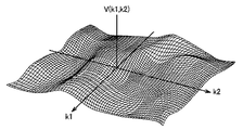
図2は、入力変数が2個の場合における入力値と出力値との関係を示す。図2の(a)は、2個の入力値の組x1(n),x2(n)と、2個の入力値の組x1(n),x2(n)のプロット点及び関数fの等高線とを示す。図2の(a)において、黒丸は、2個の入力値の組x1(n),x2(n)の各々が[0,1]の範囲で変化した場合における2個の入力値の組x1(n),x2(n)のプロット点を示し、実線は、関数fの等高線を示す。また、図2の(b)は、関数fの3次元表現である。
【0035】
この場合、サンプルデータ30は、2個の入力値の組x1(n),x2(n)を含むので、2個の入力値の組x1(n),x2(n)は、プロット点(1),(2),・・・,(S)によって表わされる。そして、プロット点(1),(2),・・・,(S)の各々が入力値として入力された場合、等高線1〜6によって表わされる出力値が得られる。この等高線1〜6によって表わされた曲面を3次元表現したものが図2の(b)に示す曲面7である。従って、プロット点(1),(2),・・・,(S)を入力値とした場合の出力値は、曲面7上に存在することになり、この発明によるプログラムは、プロット点(1),(2),・・・,(S)に対して曲面7を表わす関数fを3層ニューラルネットワーク及び高次元アルゴリズムを用いて演算する。
【0036】
曲面7は、なだらかな曲面から成る。つまり、フーリエ級数又は三角関数の級数和によって表わした方が適切な激しい振動を多く含む曲面ではなく、ガウシャン様の分布の結合により表わされる。従って、この発明によるプログラムを用いて関数fを求める演算を行なう場合、好ましくは、出力値(z(1)、z(2)、・・・、z(S))は、ガウシャン様の分布の結合により表わされるような「なだらな曲面」を構成する。
【0037】
なお、この発明において、「なだらかな曲面」とは、ガウシャン様の分布の結合により表わされる曲面を言う。
【0038】
図3は、この発明によるプログラムが入力値に対する出力演算値Z(n)を演算する3層ニューラルネットワークの概念図を示す。3層ニューラルネットワーク40は、入力層41と、中間層42と、出力層43とを含む。
【0039】
入力層41は、m1個の入力ユニット41i(i=1,・・・,m1)から成る。中間層42は、m2個の中間ユニット42j(j=1,・・・,m2)から成る。出力層43は、1個の出力ユニット431から成る。
【0040】
入力ユニット41iは、入力層41のi番目のユニットに入力される入力値xi(n)を受け、その受けた入力値xi(n)をm2個の中間ユニット42jの各々に伝達する。
【0041】
中間層42は、入力値と出力値との間の特徴抽出の主要な役割を担う層である。中間ユニット42jの内部状態、出力及び閾値をそれぞれyj,Yj,θjとし、i番目の入力ユニット41iとj番目の中間ユニット42jとの間の結合のパラメータをwijとしたとき、中間ユニット42jは、式(1)により内部状態yjを演算する。
【0042】
【数1】

即ち、中間ユニット42jは、超球面識別タイプの演算を行なう。中間ユニット42jが超球面識別タイプの演算を行なう理由については後述する。
【0044】
そして、中間ユニット42jは、演算した内部状態yjを式(2)に代入して出力Yjを演算する。
【0045】
【数2】
即ち、中間ユニット42jは、シグモイド関数により出力Yjを演算する。式(2)において、Tjは、シグモイド関数の遷移領域のスロープを調整するパラメータである。この実施の形態においては、式(2)の右辺の分母に含まれる指数関数が数値的に発散するのを防止するためにTjは、式(3)により定義される。
【0047】
【数3】
式(3)において、τjは、中間ユニット42jの出力関数の傾きを表わす。
中間ユニット42jは、出力Yjを演算すると、その演算した出力Yjを出力層43の出力ユニット431へ出力する。
【0049】
出力層43は、m2個の中間ユニット42jの各々の出力結果を適切な重み付けにより最終出力の調整を行なう。従って、出力ユニット431は、式(4)により出力演算値Z1(n)を演算する。
【0050】
【数4】
式(4)において、Wjは、j番目の中間ユニット42jとの結合重みであり、Θは、出力ユニット431の閾値である。
【0052】
なお、この発明においては、中間ユニットの個数は、最初、1個に設定され、その設定された1個の中間ユニットを用いた近似関数fを求める演算結果に応じて、1個づつ増加される。従って、出力ユニット431は、最初、中間ユニット421からの出力Y1と、結合重みW1とを式(4)に代入して出力演算値Z1(n)を演算し、中間ユニットの個数が増加されれば、その増加された中間ユニットからの出力及び増加された中間ユニットとの結合重みを用いて出力演算値Z1(n)を演算する。
【0053】
このように、3層ニューラルネットワーク40は、m1個の入力値(x1(n),・・・,xm1(n))に対して、θj,wij,τj,Wj,Θをパラメータとして1個の出力演算値Z1(n)を演算する。そして、S個のサンプル1〜Sの各々は、m1個のデータから成る入力値(x1(n),・・・,xm1(n))を含むので、3層ニューラルネットワーク40は、m1×S個の入力値に対してS個の出力演算値Z1(1),・・・,Z1(S)を演算する。
【0054】
中間ユニット42jが内部状態yjを求めるために式(1)により超球面識別タイプの演算を行なう理由について説明する。一般に、内部状態yjを求めるために式(5)により表わされる入力値xi(n)と結合のパラメータwijとの積和演算がよく使用される。
【0055】
【数5】
この場合、識別曲面の方程式yj=0は、1つの超平面を指定する。その例を図4及び図5に示す。図4は、2個の入力値の組x1(n),x2(n)を用いた場合に式(5)を用いて演算された内部状態yjを示す。また、図5は、2個の入力値の組x1(n),x2(n)を用いた場合の中間ユニットからの出力Yjを示す。
【0057】
図4に示すように、識別曲面の方程式yj=0は、1つの超平面50を指定する。そして、図5に示すように、中間ユニットの出力Yjは、超平面50を境界にして変化する曲面によって表わされる。超平面50の両側の領域51及び52は、ほぼ平坦であり、領域51及び52の各々において、更に狭い領域における特徴を表現することはできない。即ち、2個の入力値の組x1(n),x2(n)に対して演算された中間ユニットの出力Yjは、超平面50を境界にして変化するという大局的特徴を表現できるが、領域51及び52の更に狭い領域における局所的特徴を表現することができない。
【0058】
式(5)を用いて内部状態yjを演算することを超平面識別タイプの演算をすると言う。そして、超平面識別タイプの演算を行なった場合、上述したように、大局的特徴を表現できるが、1つの中間ユニットで局所的特徴を表現することはできない。局所的特徴を表現するには多数の中間ユニットを要する。
【0059】
一方、式(1)を用いて内部状態yjを演算した場合、識別曲面の方程式yj=0は、1つの超球面を指定する。その例を図6及び図7に示す。図6は、2個の入力値の組x1(n),x2(n)を用いた場合に式(1)を用いて演算された内部状態yjを示す。また、図7は、2個の入力値の組x1(n),x2(n)を用いた場合の中間ユニット42jからの出力Yjを示す。
【0060】
図6に示すように、識別球面の方程式yj=0は、1つの超球面60を指定する。そして、図7に示すように、中間ユニット42jの出力Yjは、超球面60の外側では平面であり、超球面60の内側では凸曲面になる。また、超球面60は、一般的には狭い領域に形成される。従って、中間ユニット42jの内部状態yjを超球面識別タイプの演算により求めることにより局所的特徴を表現することができる。
【0061】
上述したように、超平面識別タイプの演算により内部状態yjを求めれば、大局的特徴を表現できるが、局所的特徴を表現できない。一方、超球面識別タイプの演算により内部状態yjを求めれば、局所的特徴を表現できるが、大局的特徴を表現することができない。
【0062】
従って、理想的には、局所的特徴の表現に有利な中間ユニットと、大局的特徴の表現に有利な中間ユニットとを揃えればよいが、それぞれどれだけの個数を揃えればよいかが未知であるため超平面識別タイプの演算及び超球面識別タイプの演算を混在して行なえば、計算量が増加する。
【0063】
そこで、この発明においては、局所的特徴の表現に有利な超球面識別タイプの演算を採用し、中間ユニット42jが内部状態yj及び出力Yjを演算する際のパラメータ(θj,wij,τj)を通常の探索範囲よりも広い範囲で変化させることにより大局的特徴を表現することにした。
【0064】
2個の入力値の組x1(n),x2(n)を用いた場合、識別曲面の方程式yj=0は、式(1)より、パラメータwijを中心とし、パラメータθjを半径とする円を指定する。パラメータθj及びwijの範囲を変えた場合の関数fの変化について説明する。
【0065】
図8は、パラメータθj及びwijの範囲を局所的特徴に相応する小さな半径にした場合における識別超球面の取り得る相対的位置関係と中間ユニット42jの出力例とを示す。図9は、パラメータθj及びwijの範囲を広くした場合における識別超球面の取り得る相対的位置関係と中間ユニット42jの出力例とを示す。図10は、パラメータwij(中心)が入力変数x1,x2の定義域外に存在する小さな超球である場合における識別超球面の取り得る相対的位置関係と中間ユニット42jの出力例とを示す。
【0066】
パラメータ(w1j,w2j)(中心)が入力変数x1,x2の定義域内([0,1]2の範囲)にあって、パラメータθj(半径)の取り得る範囲が[0,0.5]程度と小さい場合(図8の(a)参照)、中間ユニット42jは、局所的特徴を反映した曲面61又は62によって表わされる出力Yjを出力する(図8の(b)参照)。
【0067】
曲面61は、パラメータ(w1j,w2j)(中心)が(0.5,0.5)であり、パラメータθj(半径)が0.1であり、Tjが0.03である場合に得られる。また、曲面62は、パラメータ(w1j,w2j)(中心)が(0.5,0.5)であり、パラメータθj(半径)が0.1であり、Tjが0.05である場合に得られる。
【0068】
このように、パラメータ(w1j,w2j)(中心)を入力変数x1,x2の定義域内に設定し、パラメータθj(半径)を小さい値にした場合、中間ユニット42jは、局所的特徴を反映した曲面61及び62によって表わされる出力Yjを出力する。
【0069】
パラメータ(w1j,w2j)(中心)が入力変数x1,x2の定義域外([−0.2,1.2]2の範囲)にあって、パラメータθj(半径)の取り得る範囲が[0,1.5]と大きい場合(図9の(a)参照)、中間ユニット42jは、曲面63又は64によって表わされる出力Yjを出力する(図9の(b)参照)。
【0070】
曲面63は、パラメータ(w1j,w2j)(中心)が(1.2,1.2)であり、パラメータθj(半径)が1.0であり、Tjが0.1である場合に得られる。また、曲面64は、パラメータ(w1j,w2j)(中心)が(1.2,1.2)であり、パラメータθj(半径)が1.0であり、Tjが0.5である場合に得られる。
【0071】
曲面63及び64は、図5に示す曲面に似た曲面である。従って、パラメータ(w1j,w2j)(中心)を入力変数x1,x2の定義域外に設定し、パラメータθj(半径)を大きい値にした場合、中間ユニット42jは、大局的特徴を反映した曲面63及び64によって表わされる出力Yjを出力する。つまり、中間ユニット42jは、近似的に超平面識別タイプの演算を行なう。このことは、超球面識別タイプの演算においてパラメータθj及びwijの範囲を局所的特徴を反映する範囲よりも広い範囲に設定することによって、中間ユニット42jは、大局的特徴を反映した出力Yjを出力できることを意味する。
【0072】
パラメータ(w1j,w2j)(中心)が入力変数x1,x2の定義域外にあって、パラメータθj(半径)が小さい場合(図10の(a)参照)、中間ユニット42jは、曲面65によって表わされる出力Yjを出力する(図10の(b)参照)。
【0073】
この場合、中間ユニット42jは、定義域全域において、ほぼゼロの値から成る曲面65を出力し、最終出力である出力演算値Z1(n)に殆ど寄与しない。
【0074】
上述したように、パラメータθj,wij及びTj(つまりτj)の範囲を変化させることにより、中間ユニット42jは、超球面識別タイプの演算において局所的特徴を反映した出力Yj(図8参照)及び大局的特徴を反映した出力Yj(図9参照)の両方を出力することが可能である。そして、超球面識別タイプの演算により局所的特徴及び大局的特徴を反映するようにしても中間ユニット42jのパラメータの数が増加することはない。従って、この発明においては、中間ユニット42jは、パラメータθj,wij及びTj(つまりτj)の範囲を通常の超球面識別タイプの演算を行なう範囲よりも広い範囲まで変化させて超球面識別タイプの演算を行ない、出力Yjを出力することにした。これが、中間ユニット42jにおいて超球面識別タイプの演算を行なうことにした理由である。
【0075】
なお、「通常の探索範囲」とは、超球面識別タイプの演算により局所的特徴のみを出力Yjに反映させるためにパラメータθj,wij及びTj(つまりτj)を変化させる範囲を言う。
【0076】
中間ユニット42jからの出力Yjは、出力ユニット431に入力され、出力ユニット431は、出力Yj及びパラメータWj,Θを式(4)へ代入して出力演算値Z1(n)を演算する。
【0077】
出力演算値Z1(n)が演算されると、サンプルデータ30に含まれる出力値z1(n)と出力演算値Z1(n)との二乗誤差の和の平均V(wij,θj,τj,Θ)が式(6)により演算される。
【0078】
【数6】
二乗誤差の和の平均V(wij,θj,τj,Wj,Θ)は、3層ニューラルネットワーク40によって演算された出力演算値Z1(n)が実際の出力値z1(n)に近い度合いを示す指標であり、出力演算値Z1(n)を評価するコスト関数である。
【0080】
この発明によるプログラムは、パラメータwij,θj,τj,Wj,Θを変化させて(中間ユニット42jのパラメータwij,θj,τjについては、局所的特徴を反映する範囲よりも広い範囲で変化させる)、出力演算値Z1(n)を演算し、出力演算値Z1(n)を式(6)に代入して演算したコスト関数V(wij,θj,τj,Wj,Θ)の関数値が所定値ε以下になるようにパラメータwij,θj,τj,Wj,Θを最適化する。この場合、この発明によるプログラムは、最初、中間ユニット42jの個数を1個に設定し(j=1)、その設定した1個の中間ユニット421を用いて最終的に演算したコスト関数V(wij,θj,τj,Wj,Θ)の関数値が所定値εよりも大きいとき、関数値が所定値ε以下になるまで中間ユニット42jの個数を1個づつ増加し、関数値が所定値ε以下になるようにパラメータwij,θj,τj,Wj,Θを最適化する。
【0081】
このパラメータwij,θj,τj,Wj,Θが最適化されれば、入力値x1(n),・・・,xm1(n)と出力値z1(n)(n=1〜S)との関係を規定する近似関数fが決定されるので、パラメータwij,θj,τj,Wj,Θを最適化することは、近似関数fを求める演算を行なうことに相当する。
【0082】
上述したように、中間ユニット42jは、パラメータwij,θj,τjを局所的特徴を反映する範囲よりも広い範囲で変化させて超球面識別タイプの演算を行なうが、パラメータwij,θj,τjを広い範囲で変化させると、コスト関数V(wij,θj,τj,Wj,Θ)において広い平坦領域を増加させることになる。図10の(a)に示すように、中心wijが入力値の定義域外にあり、半径θjが小さい場合、中間ユニット42jの出力Yjは、定義域全域においてほぼゼロとなり、最終出力である出力演算値Z1(n)に殆ど寄与しない。従って、パラメータ空間における、このような状況に対応する領域ではコスト関数V(wij,θj,τj,Wj,Θ)が平坦になってしまう。
【0083】
wij,θj,τj,Wj,Θのようなパラメータを最適化する場合によく用いられる誤差逆伝播法(BP:Error Back−Propagation Algorithm)又は焼きなまし法(SA:Simulated Annealing)のようなアルゴリズムは、広い平坦領域を含むコスト関数に対して非常に効率が悪い。広い平坦領域の出現を避けるためにコスト関数にペナルティー項を追加する方法も考えられるが、この方法では、本来のコスト関数をゆがめたり、コスト関数の評価に要する計算量を増加させることになる。
【0084】
そこで、この発明においては、広い平坦領域、及びニューラルネットワークの学習において常に問題となる複数の局所解を含むコスト関数に対して有効な最適化手法である高次元アルゴリズムを採用することにした。
【0085】
高次元アルゴリズムによるパラメータの最適化について説明する。図11は、高次元アルゴリズムによる最適化のフローチャートを示す。解くべき問題に現われる全ての最適化すべき変数qの空間を意味空間と定義する(ステップA)。そして、変数qと共役な変数pを人為的に導入し、変数pの新しい空間を定義する(ステップB)。その後、変数pの空間を意味空間に加え、意味空間を高次元化した空間を高次元空間と定義する(ステップC)。
【0086】
そして、変数q,pの高次元空間において、問題を設定する(ステップD)。最後に、高次元空間において、自律的運動によって最適解を探索し、コスト関数を最小とする最適解を検出する(ステップE)。ここで、自律的運動とは、解の存在しない領域を素速く通過し、解の存在する領域に容易に入る運動を言う。
【0087】
このように、高次元アルゴリズムは、最適化すべき変数qの意味空間を高次元化し、その高次元化した高次元空間において自律的運動を行なうことによって最適解を検出する。
【0088】
図12は、高次元アルゴリズムによる解の探索方法を示す概念図である。また、図13は、パラメータが2個(k1,k2)の場合におけるコスト関数のランドスケープを示す。図13に示すランドスケープには、多くの山及び谷が存在し、解は全ての谷の最も低い点(極小値)に対応する。従って、解を求めるためには、複雑に入り組んだ多くの山及び谷を通過して最も低い谷に到達する必要がある。
【0089】
つまり、図12に示すように、最適化すべき変数qの意味空間70において解71に到達するには、矢印72で示される経路を移動して多くの山及び谷を通過する必要がある。しかし、大きな意味空間70において小さな解71に到達するのは困難である。
【0090】
そこで、変数qと共役な変数pを追加して変数q,pの高次元空間80を定義する。この高次元空間80においては、意味空間70において解でない領域は小さく、解に相当する領域は拡大される。従って、高次元空間80においては、意味空間70における解71が解の存在する領域81に拡大され、矢印82によって示される経路を運動して領域81に容易に到達する。そして、高次元空間80では解でない領域は小さくなり、解に相当する領域は拡大されるので、矢印82によって示される経路を運動する場合、解でない領域を素速く通過し、解の存在する領域81に容易に入る。つまり、高次元空間80においては、自律的運動が行なわれて解が検出される。
【0091】
このように、探索すべき空間を高次元化すれば目的物を探索し易いことは、次の例によって明確に理解できる。例えば、長い切り口の六角形の鉛筆を探索する場合を考える。この鉛筆を正面から見ると、小さい六角形の断面が見えるだけであるが、視線をシフトすれば、その切り口の長さも見える。この「長さ」を次元と考えれば、上述した意味空間70から高次元空間80へ次元を高次元化することにより、解を探索し易くなることを容易に理解できる。
【0092】
高次元アルゴリズムは、このように探索すべき空間を高次元化し、その高次元化した高次元空間において解を探索する結果、コスト関数の局所解に捉まりにくく、かつ、コスト関数の平坦領域を素速く通過でき、大局解を容易に求めることができる。
【0093】
3層ニューラルネットワーク40により演算された出力演算値Z1(n)が実際の出力値z1(n)に近くなるように高次元アルゴリズムを用いてパラメータwij,θj,τj,Wj,Θを最適化する場合、この発明によるプログラムは、高次元空間80における変数q,pの関数であるハミルトニアンH(q,p)を用いる。このハミルトニアンH(q,p)は、運動する力学系を表わす具体的な道具であり、この具体的な道具(ハミルトニアンH(q,p))によって表わされた空間においては、意味空間70を成す変数qと、意味空間70を高次元空間80へ高次元化し、かつ、変数qと共役である変数pとを導入し易いからである。実際の力学系の場合、変数qは、運動する物体の位置を表わし、変数pは、運動する物体の速度を表わす。高次元アルゴリズムは、この力学系のアナロジーを取って最適パラメータを探索することを特徴とする最適化手法である。
【0094】
この発明の近似関数を求める問題の場合、高次元アルゴリズムによって最適化すべき変数qはq=wij,θj,τj,Wj,Θとなる(図11のステップA参照)。そして、この変数q=wij,θj,τj,Wj,Θは、運動する物体の位置に対応する。ポテンシャルエネルギーV(q)は、変数q=wij,θj,τj,Wj,Θの関数である。
【0095】
次に、変数qに共役な変数pが人為的に導入され、変数pの成す新しい空間が定義される(図11のステップB参照)。この新しい空間を意味空間に加えたものを高次元空間と定義する(図11のステップC参照)。変数pは、上述したように運動する物体の速度に対応し、変数pの関数である運動エネルギーT(p)に対応する関数を運動する力学系と同様に定義する(図11のステップD参照)。
【0096】
その後、意味空間における関数V(q)に新しい空間における関数T(p)を加えて意味空間を高次元化した高次元空間における関数H(q,p)が変数q,pによって定義される(図11のステップD参照)。
【0097】
ハミルトニアン力学系においては、運動する物体の任意の時間tにおける位置は、ハミルトニアンH(q,p)から導かれる運動方程式により決定されるため、高次元アルゴリズムにおいても同様にする。
【0098】
最後に、高次元空間において、自律的運動によって最適解を検出することは、ハミルトニアンH(q,p)から導かれる運動方程式を解いて最適化された変数qを見つけることに相当する(図11のステップE参照)。
【0099】
ポテンシャルエネルギーV(q)は、式(7)によって表わされる。
【0100】
【数7】
即ち、ポテンシャルエネルギーV(q)は、コスト関数VC(q)と拘束ポテンシャルVL(q)との和とする。この拘束ポテンシャルVL(q)は、パラメータq=wij,θj,τj,Wj,Θの探索範囲を制限するものである。そして、拘束ポテンシャルVL(q)は、式(8)によって表わされる。
【0102】
【数8】
式(8)において、cは、拘束の強さを制御するパラメータであり、この実施の形態においてはc=1に設定される。また、式(8)におけるνn(qn)は、式(9)によって表わされる。
【0104】
【数9】
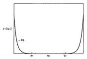
式(9)において、θ(u)は、階段関数を表わし、u=an−qn又はqn−bn>0のとき、θ(u)=1であり、u=an−qn又はqn−bn<0のとき、θ(u)=0である。
【0106】
即ち、νn(qn)は、図14に示す曲線89によって表わされ、パラメータq=wij,θj,τj,Wj,Θの探索範囲の限界を規定する。
【0107】
また、運動エネルギーT(p)は、式(10)によって表わされ、ハミルトニアンH(q,p)は、式(11)によって表わされる。
【0108】
【数10】
【数11】
その結果、系の運動を記述する運動方程式は、式(12)によって表わされる。
【0111】
【数12】
また、式(12)の下側の式の右辺に現われるコスト関数VC(q)及び拘束ポテンシャルを示す関数VL(q)のパラメータq=wij,θj,τj,Wj,Θによる微分形をそれぞれ式(13)及び式(14)に示す。
【0113】
【数13】
【数14】
ランダムに選択した初期値(q(0),p(0))を出発点とし、式(12)の2N個の一階微分方程式の組をベルレー(Verlet)法又はルンゲクッタ(Runge−Kutta)法を用いて数値的に解くことにより、系の軌道(q(t),p(t))が得られる。そして、十分な時間、軌道q(t)に沿ったコスト関数VC(q(t))を監視することにより、パラメータq=wij,θj,τj,Wj,Θの最適値を見つけることができる。
【0116】
式(12)に示す運動方程式により記述される運動系は、混合性を持ち、かつ、全エネルギーEが一定である力学系である。この場合、系は、位相空間のH(q,p)=Eを満たす等エネルギー曲面上を等しい確率で到る所を動き回ることが期待される(等重率の原理)。この等重率の原理に基づけば、系が位置qの近傍の微小体積q+dq内に滞在する時間の期待値δ(q)は、式(15)によって表わされる(ケイ、シンジョー(K.Shinjo)及びティー、ササダ(T.Sasada)著、「ハミルトニアン システムズ ウィズ メニィ ディグリー オブ フリードム:アシンメトリック モウション アンド インテンシティ オブ モウション イン フェーズ スペース(Hamiltoniansystems with many degrees of freedom:asymmetric motion and intensity ofmotion in phase space)」、フィジカル レビュー(Physical Review)E54,pp4685−4700,1996)。
【0117】
【数15】
式(15)より、自由度Nが3以上のとき、高いポテンシャル値を持つ領域では滞在時間の期待値が低く、低いポテンシャル値を持つ領域では滞在時間の期待値が高くなり、更に、この傾向は、自由度Nが大きければ大きいほど顕著になる。
【0119】
従って、高次元アルゴリズムは、このような特徴を有するハミルトニアンH(q,p)の力学系のアナロジーを取って最適解を探索することにより、上述したコスト関数の局所解に捉まりにくく、かつ、コスト関数の平坦な領域を素速く通過するという特徴を有する。
【0120】
この高次元アルゴリズムの特徴を概念的に説明する。
図15は、コスト関数の局所解に捉まる度合いを高次元アルゴリズム(HA)と焼きなまし法(SA)について比較して示す。図15の(a)は、高次元アルゴリズム(HA)の場合を示し、図15の(b)は、焼きなまし法(SA)の場合を示す。図15の(a)及び(b)において、横軸は最適化すべき変数qを表わし、縦軸はコスト関数V(q)を表わす。
【0121】
また、図16は、コスト関数の平坦領域を通過する速さを高次元アルゴリズム(HA)と焼きなまし法(SA)について比較して示す。図16の(a)は、高次元アルゴリズム(HA)の場合を示し、図16の(b)は、焼きなまし法(SA)の場合を示す。図16の(a)及び(b)において、横軸は最適化すべき変数qを表わし、縦軸はコスト関数V(q)を表わす。
【0122】
図15に示すように、高次元アルゴリズム(HA)の場合、コスト関数V(q)の谷(局所解)から抜け出す役割を運動エネルギーEが担うが、全エネルギー一定の条件より、運動エネルギーEは、コスト関数の関数値が小さい位置では大きくなる。つまり、局所解に入り込んだら運動エネルギーEが大きくなる。従って、高次元アルゴリズム(HA)は、局所解に捉まりにくい(図15の(a)参照)。一方、焼きなまし法(SA)の場合、運動は、正の絶対温度を持つことにより局所解から抜け出すことが可能であるが、この絶対温度は位置には依存しない。従って、絶対温度がコスト関数の山よりも低ければ、局所解を抜け出すことが困難である。その結果、焼きなまし法(SA)は、コスト関数の局所解に捉まり易い(図15の(b)参照)。
【0123】
また、図16に示すように、高次元アルゴリズム(HA)の場合、等速直線運動により一方の方向に運動するため、コスト関数V(q)の平坦領域を素速く通過する(図16の(a)参照)。一方、焼きなまし法(SA)の場合、ランダムウォーク(紙面の右方向及び左方向に各ステップごとにランダムに運動する)によって運動するため、コスト関数V(q)の平坦領域をなかなか通過できない(図16の(b)参照)。
【0124】
このように、高次元アルゴリズムは、コスト関数の局所解に捉まりにくく、かつ、平坦領域を素速く通過できるという特徴を有する。その結果、少ない計算量によって最適解に到達できる。
【0125】
図17は、この発明によるプログラムが入力値の組x1(n),・・・,xm1(n)と出力値z1(n)との関係を規定する近似関数fを求める演算を行なうフローチャートを示す。近似関数fを求める演算が開始されると、サンプルデータ30に含まれるm1×S個の入力値及びS個の出力値が受付けられる(ステップS1)。そして、1個に設定された中間ユニット42j(j=1)を用いて3層ニューラルネットワーク40のパラメータwij,θj,τj,Wj,Θが最適化される。
【0126】
即ち、3層ニューラルネットワーク40の中間ユニット42jのパラメータwij,θj,τjを広い探索範囲で変化させて、m1個の入力値と1個の出力値との関係を模倣する近似関数fが得られるように、3層ニューラルネットワーク40のパラメータwij,θj,τj,Wj,Θを高次元アルゴリズムを用いて最適化する(ステップS2)。これにより、パラメータwij,θj,τj,Wj,Θが最適化されれば、近似関数fが決定されるので、一連の動作は終了する。
【0127】
図18は、図17に示すステップS2の詳細な動作を説明するためのフローチャートを示す。図17に示すステップS1の後、3層ニューラルネットワーク40のパラメータwij,θj,τj,Wj,Θを初期値に設定し、超球面識別タイプの演算によりS個の出力演算値Z1(1),・・・,Z1(S)が演算される(ステップS21)。
【0128】
そして、S個の出力演算値Z1(1),・・・,Z1(S)を評価するコスト関数値が演算される(ステップS22)。その後、コスト関数値が所定値ε以下であるか否かが判定され(ステップS23)、コスト関数値が所定値ε以下であるとき一連の動作は終了する。
【0129】
一方、ステップS23において、コスト関数値が所定値ε以下でないと判定されたとき、計算回数が規定回数以下であるか否かが判定される(ステップS24)。そして、計算回数が規定回数以下であるとき、コスト関数値を低減させるためのパラメータが高次元アルゴリズムにより広い探索範囲で演算される(ステップS25)。
【0130】
即ち、式(13)及び(14)により、ステップS22において演算されたコスト関数値及び拘束条件をパラメータwij,θj,τj,Wj,Θの各々で偏微分した値を求め、式(12)により次に取るべきパラメータwij,θj,τj,Wj,Θの値を演算する。そして、その演算した値を、ステップS21における演算に用いるパラメータwij,θj,τj,Wj,Θとして用いる。
【0131】
このようにして、ステップS25の後、ステップS21〜ステップS24が繰返し実行される。
【0132】
一方、ステップS24において、計算回数が規定回数以下でないと判定されたとき、一連の繰返しのうち、最もコスト関数値が小さくなるパラメータを、その中間ユニットの最適値と固定し、3層ニューラルネットワーク40の中間ユニット42jの個数が1個増加される(ステップS26)。そして、新しく追加された中間ユニットに対してステップS21〜ステップS25が繰返し実行される。
【0133】
このように、この発明によるプログラムは、中間ユニット42jの個数が、最初、1個に設定され、その設定された1個の中間ユニット421を用いて、コスト関数値を小さくするパラメータを見つけるため、高次元アルゴリズムによりパラメータwij,θj,τj,Wj,Θを広い探索範囲で変化させて、対応するコスト関数値を次々と演算する。そして、中間ユニット42jの個数を1個にして規定回数の演算を行なっても、最も小さなコスト関数値が所定値ε以下にならないとき、中間ユニット42jの個数が1個増加され、同じ演算が繰返し実行される。中間ユニット42jの個数を2個に設定して規定回数の演算を行なっても、コスト関数値が所定値ε以下にならないとき、中間ユニット42jの個数が更に1個増加される。そして、図18に示すステップS23においてコスト関数値が所定値ε以下であると判定されるまで、高次元アルゴリズムによる新たなパラメータの探索と中間ユニット42jの個数の増加とが繰返し実行される。
【0134】
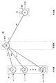
図17に示すステップS2が最初に実行される場合、中間層42の中間ユニット42jの個数は1個に設定されているので、中間層42は、中間ユニット421のみによって出力Y1を演算する。図19は、中間ユニットの個数を1個に設定した場合の3層ニューラルネットワーク40の概念図を示す。従って、3層ニューラルネットワーク40は、図19に示す入力層41、中間層42A及び出力層43によって出力演算値Z1(n)を演算する。
【0135】
この場合、中間ユニット421は、入力層41の入力ユニット41i(i=1,・・・,m1)からそれぞれ入力値x1(n),・・・,xm1(n)(n=1〜S)を受け、その受けた入力値x1(n),・・・,xm1(n)(n=1〜S)と結合のパラメータw1,1,w2,1,wm1,1と閾値θ1とを式(1)に代入して内部状態y1を演算する。そして、中間ユニット421は、演算した内部状態y1及びパラメータT1を式(2)に代入して出力Y1を演算し、その演算した出力Y1を出力層43の出力ユニット431へ出力する。
【0136】
出力ユニット431は、中間ユニット421から受けた出力Y1と結合重みW1と閾値Θとを式(4)に代入して出力演算値Z1(n)を演算する。つまり、パラメータ(wi1,θ1,τ1,W1,Θ)11を用いて出力演算値Z11(n)が演算される。なお、パラメータ(wi1,θ1,τ1,W1,Θ)11及び出力演算値Z11(n)の添字{11}のうち、前者の{1}は中間ユニット42jの個数を表わし、後者の{1}は1回目に設定されたパラメータであることを表わす。
【0137】
コスト関数VC(q)は、入力値x1(n),・・・,xm1(n)(n=1〜S)と出力値z1(n)との関係を規定する近似関数fを求める演算においては式(6)によって表わされる。従って、演算された出力演算値Z11(n)及び実際の出力値z1(n)が式(6)に代入されてコスト関数V((wi1,θ1,τ1,W1,Θ)11)のコスト関数値V11が演算される(図18のステップS22参照)。なお、コスト関数値V11の添字{11}の意味は、パラメータ(wi1,θ1,τ1,W1,Θ)11及び出力演算値Z11(n)の添字の意味と同じである。
【0138】
そして、コスト関数値V11が所定値ε以下でないとき、コスト関数値V11よりも小さいコスト関数値V12を求めるためのパラメータ(wi1,θ1,τ1,W1,Θ)12を高次元アルゴリズムにより求める(図18のステップS25参照)。その後、パラメータ(wi1,θ1,τ1,W1,Θ)12を用いてS個の出力演算値Z12(n)が演算され(図18のステップS21参照)、式(6)によりコスト関数値V12が演算される(図18のステップS22参照)。
【0139】
そして、コスト関数値V12が所定値ε以下であるか否かが判定され(図18のステップS23)、コスト関数値V12が所定値ε以下でないとき、既に演算された最小のコスト関数値よりも更に小さいコスト関数値V1h(h:h≦kの自然数、k:規定回数)を求めるためのパラメータ(wi1,θ1,τ1,W1,Θ)1hが演算される(図18のステップS25参照)。
【0140】
このように、計算回数が規定回数k以下であるとき、高次元アルゴリズムによりなるべく小さいコスト関数値V1h(hは、k以下の自然数)を見つけるためのパラメータ(wi1,θ1,τ1,W1,Θ)1hの値が演算され、その演算されたパラメータ(wi1,θ1,τ1,W1,Θ)1hを用いて新たなコスト関数値V1hが演算され、これが次々と繰返される。つまり、高次元アルゴリズムによりパラメータ(wi1,θ1,τ1,W1,Θ)を変化させて対応するコスト関数値を監視しながら最も小さいコスト関数値と、最も小さいコスト関数値に対応するパラメータとを探す。
【0141】
そして、計算回数が規定回数に達すると、中間ユニット42jの個数は、1個増加され、2個に設定される(図18のステップS26参照)。
【0142】
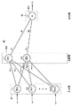
図20は、中間ユニットの個数を2個に設定した場合の3層ニューラルネットワーク40の概念図を示す。従って、3層ニューラルネットワーク40は、図20に示す入力層41、中間層42B及び出力層43によって出力演算値Z21(n)を演算する。
【0143】
この場合、中間ユニット421は、入力層41の入力ユニット41i(i=1,・・・,m1)からそれぞれ入力値x1(n),・・・,xm1(n)(n=1〜S)を受け、その受けた入力値x1(n),・・・,xm1(n)(n=1〜S)と結合のパラメータw1,1,w2,1,wm1,1と閾値θ1とを式(1)に代入して内部状態y1を演算する。そして、中間ユニット421は、演算した内部状態y1及びパラメータT1を式(2)に代入して出力Y1を演算し、その演算した出力Y1を出力層43の出力ユニット431へ出力する。なお、パラメータw1,1,w2,1,wm1,1、θ1及びTjは、最も小さいコスト関数値を記録したときのパラメータ(wi1,θ1,τ1,W1)1kに固定される。
【0144】
また、中間ユニット422は、入力層41の入力ユニット41i(i=1,・・・,m1)からそれぞれ入力値x1(n),・・・,xm1(n)(n=1〜S)を受け、その受けた入力値x1(n),・・・,xm1(n)(n=1〜S)と結合のパラメータw1,2,w2,2,wm1,2と閾値θ2とを式(1)に代入して内部状態y2を演算する。そして、中間ユニット422は、演算した内部状態y2及びパラメータT2を式(2)に代入して出力Y2を演算し、その演算した出力Y2を出力層43の出力ユニット431へ出力する。
【0145】
出力ユニット431は、中間ユニット421から受けた出力Y1と中間ユニット422から受けた出力Y2と結合重みW1,W2と閾値Θとを式(4)に代入して出力演算値Z21(n)を演算する。
【0146】
そして、出力演算値Z21(n)を用いてコスト関数値V21が演算され、中間ユニット421のみを用いた場合と同様の演算が繰返し実行される。中間ユニット42jの個数を2個に設定し、高次元アルゴリズムによりパラメータ(wi1,θ1,τ1,W1,Θ)2hを変化させて小さいコスト関数値V2hを見つける計算を規定回数kまで繰返し実行してもコスト関数値V2hが所定値ε以下にならないとき、中間ユニット42jの個数が更に1個増加され、中間ユニット42jの個数を2個に設定した場合と同様の演算が繰返し実行される。
【0147】
このように、中間ユニット42jの個数がある値に設定されると、その設定された個数の中間ユニット42jを用いて演算された出力演算値Z(n)を評価するコスト関数値を小さくする最適値を求めるために、新たなパラメータ(wij,θj,τj,Wj,Θ)が高次元アルゴリズムにより次々と演算される。そして、新たなパラメータの演算を規定回数まで行なってもコスト関数値が所定値ε以下にならないとき、中間ユニット42jの個数を1個増加してコスト関数値を小さくするように新たなパラメータ(wij,θj,τj,Wj,Θ)が高次元アルゴリズムにより次々と演算される。
【0148】
従って、この発明によるプログラムは、3層ニューラルネットワーク40の中間ユニット42jの個数を1個づつ増加させながらパラメータ(wij,θj,τj,Wj,Θ)を最適化することを特徴とする。
【0149】
なお、上記においては、中間ユニット42jの個数は、最初、「1」個に設定されると説明したが、この発明においては、これに限らず、最初、複数に設定されてもよい。つまり、この発明においては、中間ユニット42jの個数は、最初、1個以上の初期値に設定されればよい。
【0150】
3層ニューラルネットワーク40のパラメータ(wij,θj,τj,Wj,Θ)は、中間ユニット42jの個数が増加するごとに(m1+3)個づつ増加する。例えば、中間ユニット42jの個数が1個から2個に増加したとき、全体のパラメータは、(wi1,θ1,τ1,W1,Θ)から(wi1,θ1,τ1,W1;wi2,θ2,τ2,W2,Θ)へ(m1+3)個増加する。従って、中間ユニット42jの個数を1個づつ増加してパラメータ(wij,θj,τj,Wj,Θ)を最適化することは、パラメータの数を所定数づつ増加してパラメータ(wij,θj,τj,Wj,Θ)を最適化することに相当する。そして、パラメータの数が増加される前の所定数のパラメータのうち、パラメータ(wi1,θ1,τ1,W1)の値を固定し、増加されたパラメータ(wi2,θ2,τ2,W2)とパラメータΘのうち、超球面識別タイプの演算を行なう中間ユニット422のパラメータ(wi2,θ2,τ2)を広い探索範囲で変化させて出力演算値Z1(n)を演算する。この場合、図17に示すステップS2では、パラメータの個数を所定数の初期値に設定してパラメータの最適化を行なう。
【0151】
従って、この発明によるプログラムは、3層ニューラルネットワークのパラメータの数を所定数づつ増加してパラメータを最適化することを特徴とする。
【0152】
近似関数fを求める演算を行なう場合における3層ニューラルネットワーク40の効果について説明する。即ち、3層ニューラルネットワーク40の中間ユニット42jにおいて超球面識別タイプの演算を行なう場合の効果について説明する。
【0153】
図21は、二入力−一出力の3つのテスト関数の等高線を示す。図21の(a)は、テスト関数zをz=−0.76x1+0.19x2+0.78としたときの等高線を示す。図21の(b)は、テスト関数zをz=sin(πx1)・sin(πx2)としたときの等高線を示す。図21の(c)は、テスト関数zをz=0.5exp{−5(x1−0.2)2−5(x2−0.2)2}+0.9exp{−5(x1−0.8)2−10(x2−0.6)2}としたときの等高線を示す。図21の(a),(b),(c)において、横軸及び縦軸は入力変数x1,x2を表わす。
【0154】
また、各学習条件は、次に示すとおりである。
【0155】
問題(i)の場合、次の結果が得られた。
<1>超平面識別ネットワーク
獲得した中間ユニットの個数=1
平均学習回数≒11,507回
<2>超球面識別ネットワーク
獲得した中間ユニットの個数=1
平均学習回数≒64,103回
図21の(a)に示すように、このテスト関数の等高線は線型であり、超平面識別ネットワークに明らかに有利な問題である。しかし、超球面識別ネットワークにおいても、1個の中間ユニットで比較的厳しい要求精度(ε≦0.003)を達成していることから、パラメータの探索範囲を広くすることにより、局所的特徴のみならず、大局的特徴も反映させることができ、写像能力が強化されることが解る。
【0156】
一方、超球面識別ネットワークは、平均学習回数が超平面識別ネットワークの6倍程度多い。これは、パラメータの探索範囲を広くしたことが原因しているが、明らかに不利なケースにも拘わらず、高々6倍程度の増加に留まっている。
【0157】
次に、問題(ii)の結果を示す。
<1>超平面識別ネットワーク
獲得した中間ユニットの個数=8
平均学習回数≒393,829回
<2>超球面識別ネットワーク
獲得した中間ユニットの個数=1
平均学習回数≒12,045回
図21の(b)に示すように、このテスト関数の等高線は、閉じた曲線であり、超球面識別ネットワークに明らかに有利な場合である。超平面識別ネットワークについては、要求精度をε≦0.03に上げると学習の収束が急速に困難になったため、ε≦0.05とした。必要な中間ユニットの個数は、超平面識別ネットワークが8個、超球面識別ネットワークが1個という結果であり、これから、写像能力は、超球面識別ネットワークの方が各段に優れていることが解る。
【0158】
平均学習回数に関しても、8倍の中間ユニット数(パラメータ数)を要する超平面識別ネットワークでは約33倍多く、超平面識別ネットワークは、局所的特徴の表現には効率が悪いことが解る。
【0159】
最後に、問題(iii)の結果を示す。
<1>超平面識別ネットワーク
獲得した中間ユニットの個数=6
平均学習回数≒264,706回
<2>超球面識別ネットワーク
獲得した中間ユニットの個数=2
平均学習回数≒2,665回
図21の(c)に示すように、このテスト関数は、非対称な閉じた等高線を持ち、現実の応用問題にありそうな一例である。超平面識別ネットワークは、要求精度ε≦0.01を達成するのが困難であったため、ε≦0.03とした。
【0160】
中間ユニットの個数は、超球面識別ネットワークが2個であり、超平面識別ネットワークが6個である。その結果、この場合も超球面識別ネットワークの方が写像能力が高いことが解る。平均学習回数も、超平面識別ネットワークは、超球面識別ネットワークの100倍近く多い。
【0161】
このように、パラメータの探索範囲を適切に拡大した超球面識別ネットワークを高次元アルゴリズムで学習する方法は、一般に、超平面識別ネットワークの場合よりも少ないパラメータ数で要求精度を達成できる高い写像能力を持ち、かつ、学習性能も良好であることが確認された。
【0162】
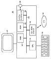
図17に示すステップS1,S2及び図18に示すステップS21〜S26を備えるプログラムは、図22に示すパーソナルコンピュータによって実行される。図22は、パーソナルコンピュータの概略ブロック図である。パーソナルコンピュータ90は、データバスBSと、CPU91と、RAM(Random Access Memory)92と、ROM(Read Only Memory)93と、シリアルインタフェース94と、端子95と、CD−ROMドライブ96と、ディスプレイ97と、キーボード98とを備える。
【0163】
CPU91は、ROM93に格納されたプログラムをデータバスBSを介して読出す。また、CPU91は、シリアルインタフェース94、端子95及びインターネット網を介して取得したプログラム、またはCD(Compact Disk)99からCD−ROMドライブ96を介して読出したプログラムをROM93に格納する。更に、CPU91は、キーボード98から入力されたユーザからの指示を受付ける。
【0164】
RAM92は、CPU91が上述した近似関数fを求める演算を行なう際のワークメモリである。ROM93は、プログラム等を格納する。シリアルインタフェース94は、データバスBSと端子95との間でデータのやり取りを行なう。
【0165】
端子95は、ケーブルによってパーソナルコンピュータ90をインターネットに接続するためのインタフェース(図示せず)に接続するための端子である。CD−ROMドライブ96は、CD99に記録されたプログラムを読出す。ディスプレイ97は、各種の情報を視覚情報としてユーザに与える。キーボード98は、ユーザからの指示を受付ける。
【0166】
CPU91は、キーボード98を介して入力されたユーザの指示に応じて、ROM93に格納されたプログラムを読出し、その読出したプログラムを実行する。そして、CPU91は、図17及び図18に示すフローチャートに従って近似関数fを求める演算を行ない、最適化されたパラメータをディスプレイ97に表示する。
【0167】
この発明によるプログラムは、CD99からCD−ROMドライブ96を介してCPU91によって読み込まれてROM93に格納され、またはシリアルインタフェース94、端子95及びインターネットを介して取得されてROM93に格納される。
【0168】
このように、ユーザは、この発明によるプログラムをパーソナルコンピュータ90により実行して近似関数fを求める演算を行なうことができる。
【0169】
上述したように、この発明によるプログラムが入力値x1(n),・・・,xm1(n)(n=1〜S)と出力値z1(n)との関係を規定する近似関数fを求める演算を行なう場合、サンプルデータ30の元になる集合10に含まれる入力値(x1(1),・・・,xm1(1))、(x1(2),・・・,xm1(2))、・・・、(x1(S),・・・,xm1(S))、・・・、(x1(M),・・・,xm1(M))及び集合20に含まれる出力値(z(1)、z(2)、・・・、z(S)、・・・、z(M))は、例えば、量子井戸構造における井戸層の幅dw1、井戸層の電子密度nw1、バリア層の高さWd2及びバリア層の幅db等から成る入力値と、量子井戸構造における粒子(電子及び正孔)のエネルギー準位Ew1から成る出力値として取得される。
【0170】
そこで、井戸層の幅dw1、井戸層の電子密度nw1、バリア層の高さWd2及びバリア層の幅db等から成る入力値(x1(1),・・・,xm1(1))、(x1(2),・・・,xm1(2))、・・・、(x1(S),・・・,xm1(S))、・・・、(x1(M),・・・,xm1(M))と、エネルギー準位Ew1から成る出力値(z(1)、z(2)、・・・、z(S)、・・・、z(M))とを取得する方法について説明する。
【0171】
[サンプルデータの取得方法]
エネルギー準位Ew1は、量子井戸構造における粒子の自己相互作用を考慮して演算される。
【0172】
図23は、量子準位演算プログラムが演算の対象とする量子井戸の概念図である。縦軸はエネルギーを示し、横軸は位置を示す。量子井戸100は、バリア層101,102と井戸層103とから成る。井戸層103に閉じ込められた電子はエネルギー準位104を形成する。
【0173】
この発明においては、粒子の相互作用を含まないシュレディンガー方程式を解いて1つの量子井戸100における波動関数Ψを求める。そして、求めた波動関数Ψから出発して、変分法の原理に基づき系全体のエネルギーを最小化する波動関数を求める。この場合、系全体のエネルギーは、粒子の相互作用を非線形項として含むハミルトニアンの期待値を、与えられた波動関数に対して計算したものとして定義される。その後、量子井戸100の一方のバリア層101の端から他方のバリア層102の端までを複数のポイントx1〜xN(Nは自然数)に分割し、その分割した各ポイントxi(1≦i≦N)に対応して波動関数ΨをN個の波動関数Ψ1,・・・,Ψi,・・・,ΨNに離散化する。この場合、ポイントx1〜xNの各々と隣接するポイントとの間の距離は全て等しいように位置x1〜xNが決定される。
【0174】
波動関数Ψを波動関数Ψ1,・・・,Ψi,・・・,ΨNへ離散化すると、量子井戸100の系全体のエネルギーが最小となるように、波動関数Ψ1,・・・,Ψi,・・・,ΨNの各々を演算する。そして、演算した波動関数Ψ1,・・・,Ψi,・・・,ΨNを用いて系の全体エネルギーを求める。
【0175】
このように、粒子の相互作用を含まないシュレディンガー方程式を解いて求めた波動関数ΨをN個に離散化し、系全体のエネルギーが最小となるように、離散化した波動関数Ψ1,・・・,Ψi,・・・,ΨNの各々を演算する。
【0176】
以下、粒子の相互作用を含まないシュレディンガー方程式を解いて求めた波動関数を変分法の原理に適用して系全体のエネルギーを演算する際に、ハミルトニアンに取り入れられる非線形項として粒子のクーロン相互作用を用いた場合について説明する。
【0177】
図24は、量子準位演算プログラムを構成する各ステップを示すフローチャートである。量子準位演算プログラムが実行されると、量子井戸100に閉じ込められた電子の自己相互作用のない場合の波動関数が演算される(ステップS100)。即ち、運動エネルギーの項と外部電界によるポテンシャル項とから成るハミルトニアンを用いて電子の初期の波動関数Ψが演算される。この演算は、転送行列法、S行列法、及び狙い撃ち法のいずれかを用いて行われる。
【0178】
そして、最小化される系全体のエネルギーを示す式は式(16)により与えられる。
【0179】
【数16】
式(16)の右辺の第2項は、自己相互作用を含むクーロン相互作用項である。そして、ε(x)は、位置xにおける誘電定数であり、−e及びmは、それぞれ、電子の電荷及び質量である。また、d(y)は、位置yにおける固定ドナーの体積密度であり、固定ドナーは+eの電荷を有するものと仮定している。即ち、コンピュータによる計算のために、イオン化されたドナーは、自由電子により+eの電荷を運ぶものと仮定した。
【0181】
式(16)は、量子井戸100の系全体のエネルギーを表わすが、式(16)を用いて演算することは困難であるので、空間を離散化するとともに系全体に存在する粒子数で規格化することとした。即ち、ステップS100で求めた波動関数ΨをN個の波動関数Ψ1,・・・,Ψi,・・・,ΨNに離散化するとともに系全体の粒子数で規格化することにより、式(16)から式(17)が得られる。
【0182】
【数17】
式(17)において、Ntは規格化因子であり、Neは電子数である。また、Vi’は、クーロンポテンシャルである。
【0184】
式(17)は、系に存在する1つの電子あたりのエネルギーを表わし、以下では、最適化問題の用語に合わせて「コスト関数」と呼ばれる。そして、式(17)を離散化したN個の波動関数Ψ1,・・・,Ψi,・・・,ΨNの各々によって偏微分してN個の導関数を演算する。即ち、式(18)が得られる。
【0185】
【数18】
式(18)において、Eintは1粒子当たりの非線形の相互エネルギーを意味する。そして、式(16)から式(17)及び式(18)を求めることは、コスト関数及びコスト関数の導関数を計算すること(ステップS102)に相当する。
【0187】
なお、式(18)は、式(17)の両辺を波動関数Ψ1,・・・,Ψi,・・・,ΨNの各々によって偏微分したものではなく、式(17)の自己相互作用を考慮したハミルトニアンH’を波動関数Ψ1,・・・,Ψi,・・・,ΨNの各々によって偏微分したものになっているが、その理由は次の理由による。
【0188】
量子準位演算プログラムは、自己相互作用を考慮して量子井戸100の井戸層103に閉じ込められた電子の系全体のエネルギーが最小になるように波動関数を計算することを目的とするため、式(17)の全体を波動関数Ψ1,・・・,Ψi,・・・,ΨNの各々によって偏微分するのではなく、自己相互作用を考慮したハミルトニアンH’を波動関数Ψ1,・・・,Ψi,・・・,ΨNの各々によって偏微分することにより自己相互作用の影響を最大限に反映して演算することにしたものである。
【0189】
従って、ステップS102においては、コスト関数(式(17))に離散化した波動関数Ψ1,・・・,Ψi,・・・,ΨNを代入して系全体のエネルギーS{(Ψi)}を演算し、コスト関数の導関数が自己相互作用を考慮したハミルトニアンH’を波動関数Ψ1,・・・,Ψi,・・・,ΨNの各々によって偏微分することにより演算される(式(18))。
【0190】
その後、ステップS102において演算したN個の導関数及び次式(19)を用いて新しい波動関数を演算する(ステップS104)。
【0191】
【数19】
式(19)において、ηは、量子準位演算プログラムによる最小エネルギーの演算が収束するようにするためのスケーリングファクターである。また、式(19)の右辺第2項は、自己相互作用を考慮したハミルトニアンH’を波動関数Ψの各成分よって偏微分して式(18)を演算し、その演算した式(18)に波動関数Ψoldを代入して演算される。
【0193】
式(19)による新しい波動関数Ψi newは、既に演算された波動関数Ψi oldに自己相互作用による変化分(式(19)の右辺第2項)を加算したものである。従って、新しい波動関数Ψi newは、自己相互作用の変化分を反映して演算される。そして、新しい波動関数Ψi newは、離散化したN個の波動関数Ψ1,・・・,Ψi,・・・,ΨNの各々に対して演算される。
【0194】
式(19)により新しい波動関数Ψi newが演算されると、その新しい波動関数Ψi newを式(17)の波動関数Ψiに代入して、新しい波動関数によるコスト関数(式(17))及びその導関数(式(18))が演算される(ステップS106)。
【0195】
そして、コスト関数が増加するか否かにより、またはステップS106において演算したN個の導関数の全てが零であるか否かを判定することにより、系全体のエネルギーが収束するか否かが判定される(ステップS108)。
【0196】
ステップS108において、コスト関数が増加しないとき、又はN個の導関数の全てが零でないとき、系全体のエネルギーは収束しないと判定され、ステップS104,S106,S108が繰返し実行される。これは、コスト関数が増加しないとき、コスト関数の増加分が零かコスト関数が減少していることを示し、系全体のエネルギーが更に減少する可能性があるからであり、コスト関数の導関数が零でないとき、コスト関数が変化していることを示し、この場合も系全体のエネルギーが更に減少する可能性があるからである。
【0197】
一方、ステップS108において、コスト関数が増加したとき、またはN個の導関数の全てが零であるとき、系全体のエネルギーが収束したと判定される。そして、1ステップ前の波動関数を出力する(ステップS110)。
【0198】
例えば、ステップS104,S106,S108を5回繰返して実行し、5回目にステップS108においてコスト関数が増加、又はN個の導関数の全てが零になったとすると、4回目にステップS104において式(19)を用いて演算したN個の成分をステップS110において出力する。5回目にステップS108においてコスト関数が増加、又はN個の導関数が全て零になったということは、ステップS104において4回目に演算した波動関数を用いて、ステップS106において演算したコスト関数が最小になったことを意味するからである。
【0199】
ステップS110において、系全体のエネルギーを最小にするN個の成分が決定されると、その決定されたN個の成分から成る波動関数(最終的な波動関数)と、自己相互作用を考慮したハミルトニアンである式(20)を用いて系全体のエネルギーを演算し(ステップS112)、全体の演算動作が終了する。
【0200】
【数20】
上述した各ステップのうち、ステップS102,S104,S106,S108,S110は1つの粒子に対する動作を表わす。従って、量子準位演算プログラムは、系全体のエネルギーを最小とするようにN個の成分を決定するとき、1つの粒子に着目し、その1つの粒子に対する波動関数において自己相互作用による影響が最も小さくなるようにN個の成分を決定することを第1の特徴とする。そして、1つの粒子に対する波動関数が決定されると、その決定された波動関数を系全体の粒子に適用して系全体のエネルギーを演算することを第2の特徴とする。
【0202】
その結果、量子井戸100のバリア層101,102又は井戸層103へのドーピング量の増加に起因して井戸層103に閉じ込められる電子数が増加し、電子の相互作用による影響が大きくなっても系全体のエネルギーが収束するように演算できる。
【0203】
以下、量子準位演算プログラムを用いて演算した例について具体的に説明する。
【0204】
図25は、量子準位演算プログラムが演算の対象とする量子井戸の具体例である。縦軸はエネルギーを示し、横軸はバリア層101,102及び井戸層103の厚み方向の距離zを示す。2つのバリア層101,102の各々は、35モノレイヤー(=10nm)のAl0.2Ga0.8Asから成り、井戸層103は、35モノレイヤー(=約10nm)のGaAsから成る。そして、伝導帯側のバンドの不連続値ΔEc(=Ec1−Ec2)は167meVである。
【0205】
図25に示す系において井戸層103であるGaAsのボトムエッジから28.25795meVの位置に第1準位E1が形成され、その第1準位E1を占める電子の初期の波動関数が波動関数Ψである。
【0206】
以下、井戸層103にドナーをドーピングした場合(「井戸ドーピング」と言う。)、及びバリア層101,102にドナーをドーピングした場合(「バリアドーピング」と言う。)について説明する。そして、ドーピングされたドナーは全て活性化され、自由電子の総数は、ドナーの総数に等しいと仮定する。
【0207】
また、バリア層101,102及び井戸層103の各モノレイヤーを10ポイントに分割する。即ち、波動関数Ψを1051個の波動関数Ψ1,・・・,Ψi,・・・,Ψ1051に離散化する。
【0208】
更に、バリア層101,102及び井戸層103から成る量子井戸100の両端では波動関数は零であると近似している。
【0209】
更に、式(19)のスケーリングファクターηを−1.15×10⁷に固定して計算した。このスケーリングファクターηの値は、あくまで1モノレイヤー当たり10ポイントに分割した場合の値であり、他の分割数の場合には、他の値が用いられる。例えば、1モノレイヤー当たり20ポイントに分割したのであれば、η=−2.30×10⁷が用いられる。また、スケーリングファクターηの値としては、これらの値以外の値も想定される。
【0210】
図26は、井戸ドーピングを行なった場合の計算結果をドーピング量に対して示したものである。図26の(a)〜(d)の各々において、縦軸はエネルギーを示し、横軸はバリア層101,102及び井戸層103の厚み方向の距離zを示す。図26の(a)は、ドーピング量が1.0×1018cm−3の場合を示し、図26の(b)は、ドーピング量が5.0×1018cm−3の場合を示し、図26の(c)は、ドーピング量が8.0×1018cm−3の場合を示し、図26の(d)は、ドーピング量が1.0×1019cm−3の場合を示す。また、図26の(a)〜(d)において波動関数Ψ0は初期の波動関数であり、記号Ew1〜Ew4は基底状態のエネルギー値を示し、記号Ψw1〜Ψw4は上述した量子準位演算プログラムを用いて計算された波動関数を示す。
【0211】
量子準位演算プログラムを用いて4つのドーピング量に対する計算を行なった結果、その計算時間は30秒以下と非常に短かった。
【0212】
井戸ドーピングにおいては、電子及びドナーは、両方とも井戸層103に存在するため、電子とドナーとの間で電荷の打消しが起こり、これが量子井戸の外側におけるバンドの曲がりを抑制する。そして、これは、高いドーピング量においても当てはまる。
【0213】
また、計算された波動関数のひずみは小さいことが解かった。更に、基底状態のエネルギーEw1〜Ew4の変化は、イオン化された不純物(ドナー)及び電子間の相互作用による電子のポテンシャルに起因するが、この変化は、そう大きくないのに対し、井戸層103におけるバンドの曲がりがドーピング量の増加に伴い大きくなる。
【0214】
表1は、井戸ドーピングにおいて、量子準位演算プログラムを用いて計算した基底状態のエネルギー値を従来のS−P法を用いた計算結果と比較して示す。
【0215】
【表1】
表1から明らかなように、ドーピング量が1.0×10¹⁸〜1.7×1018cm−3の範囲においては、量子準位演算プログラムを用いた計算結果は、従来のS−P法による計算結果と良い一致を示し、その差は、殆ど無視できる程度の1.3×10⁻⁴%以下である。
【0217】
また、従来のS−P法は、1.8×1018cm−3以上のドーピング量に対して発散するのに対し、量子準位演算プログラムを用いた計算結果は、少なくとも1.0×1019cm−3のドーピング量までは確実に収束することがわかった(数値が得られていることは収束していることを示す。以下同じ。)。
【0218】
このように、量子準位演算プログラムを用いた計算方法は、井戸層103へドーピングした場合において、ドーピング量の低い領域では従来のS−P法による計算結果と良い一致を示し、高いドーピング量の範囲まで収束した計算結果を示す。その結果、量子準位演算プログラムを用いることにより、高いドーピング量の範囲まで基底状態のエネルギー値を得ることができる。
【0219】
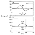
図27は、バリアドーピングを行なった場合の計算結果をドーピング量に対して示したものである。図27の(a)〜(d)において、縦軸はエネルギーを示し、横軸はバリア層101,102及び井戸層103の厚み方向の距離zを示す。また、図27の(a)〜(d)において、記号Ψ0,Ψw1〜Ψw4,Ew1〜Ew4は、図26の(a)〜(d)における意味と同じである。更に、図27の(a)は、ドーピング量が1.0×1017cm−3の場合を示し、図27の(b)は、ドーピング量が3.0×1017cm−3の場合を示し、図27の(c)は、ドーピング量が5.0×1017cm−3の場合を示し、図27の(d)は、ドーピング量が7.0×1017cm−3の場合を示す。
【0220】
この場合も、計算時間は30秒以下であった。バリア層101,102へのドーピング量が増加するに伴い波動関数Ψw1〜Ψw4のひずみが増加する。これは、次の理由による。バリアドーピングにおいては、閉じ込められた電子は井戸層103に存在し、ドナーはバリア層101,102に存在するため、井戸層103の電子は、電子間の相互作用による反発力とバリア層101,102に存在するドナーからの引力とにより両側に存在するバリア層101,102の方へ拡がろうとする。そして、バリア層101,102へのドーピング量が増加するに従ってバリア層101,102に存在するドナーからの引力が増加するので、井戸層103における電子の拡がりは増加する。その結果、バリア層101,102へのドーピング量が増加するに従って波動関数Ψw1〜Ψw4のひずみが増加する。
【0221】
また、バリアドーピングの場合、井戸ドーピングの場合に比べてバンドの曲がりが大きくなる。これは、次の理由による。イオン化されたドナーによる電子のポテンシャルは、井戸層103のボトムにおけるバンド端のポテンシャルを増加させる。一方、電子とドナーとは空間的に分離されているので、イオン化されたドナーからの電気的な影響を除去しようとする電子の働きは低下する。その結果、井戸層103からバリア層101,102へ電界が及び、バンドの曲がりが大きくなる。
【0222】
表2は、バリアドーピングにおいて、量子準位演算プログラムを用いて計算した基底状態のエネルギー値を従来のS−P法を用いた計算結果と比較して示す。
【0223】
【表2】
表2から明らかなように、ドーピング量が1.0×10¹⁷〜5.0×1017cm−3の範囲においては、量子準位演算プログラムを用いた計算結果は、従来のS−P法による計算結果と良い一致を示す。そして、量子準位演算プログラムを用いた計算方法は、従来のS−P法では収束しない6.0×1017cm−3,7.0×1017cm−3のドーピング量において収束する。
【0225】
このように、量子準位演算プログラムを用いた計算方法は、バリア層101,102へドーピングした場合において、ドーピング量の低い領域では従来のS−P法による計算結果と良い一致を示し、高いドーピング量の範囲まで収束した計算結果を示す。その結果、量子準位演算プログラムを用いることにより、高いドーピング量の範囲まで基底状態のエネルギー値を得ることができる。
【0226】
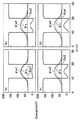
図28は、ドーピング量が2.0×1018cm−3の井戸ドーピングを行なった場合において、量子準位演算プログラムを用いた計算結果を従来のS−P法による計算結果と比較して示す。図28の(a),(b)において、縦軸はエネルギーであり、横軸はバリア層101,102及び井戸層103の厚み方向の距離zである。図28の(a)は、従来のS−P法による計算結果を示し、図28の(b)は、量子準位演算プログラムを用いた計算結果を示す。
【0227】
記号Ψc,Ψivtは、波動関数を示し、記号Vc,Vivtはバンド端のポテンシャルを示す。
【0228】
従来のS−P法は、シュレディンガー方程式の解法とポアソン方程式の解法とを繰返す過程において、小さなバランスのずれや計算のエラーが増幅され、その結果、計算ステップの進行に対して波動関数Ψcが振動する。
【0229】
これに対して、量子準位演算プログラムを用いた計算方法は、図24に示すステップS104,S106,S108の繰返しにおいて、波動関数が本当の解に近づくに従って式(19)による補正が小さくなり、その結果、波動関数Ψivtは収束する。
【0230】
上記においては、1モノレイヤー当たりの分割数が10ポイントの場合について説明したが、この分割数を変化させた場合について図29に示す。縦軸は基底状態のエネルギーを表わし、横軸は1モノレイヤー当たりの分割数を表わす。また、曲線105(実線で示される)は、量子準位演算プログラムを用いた計算結果であり、曲線106(点線で示される)は、従来のS−P法による計算結果である。なお、ドーピングは、井戸層103へ行なわれ、ドーピング量は1.0×1018cm−3である。
【0231】
両方の方法において、分割数が増加するに従って基底状態のエネルギー値が小さくなり、空間をより小さく分割した方が正確な波動関数が得られることが解った。また、空間の分割数に関しては、量子準位演算プログラムを用いた計算方法は従来のS−P法による計算方法と大きな差がないことが解かった。
【0232】
上述した井戸ドーピング及びバリアドーピングにおける計算においては、初期状態を狙い撃ち法(Shooting Method)により求めた初期状態を用いた。
【0233】
表3は、井戸ドーピング及びバリアドーピングにおいて、数学的に厳密な波動関数を用いた場合の、量子準位演算プログラムを用いた計算結果を示す。初期状態として採用した厳密な波動関数に対応するエネルギー値は、28.27683meVである。
【0234】
【表3】
その結果、初期状態として採用した厳密な波動関数に対応するエネルギー値として28.27683meVのエネルギー値を用いた場合の方が、各ドーピング量に対するエネルギー値は大きくなることが解かった(表1及び表2参照)。しかし、その差は、殆ど1.5%であり、実際の半導体材料における量子準位の見積もりにおいては許容される範囲である。従って、量子準位演算プログラムにおいては、狙い撃ち法(Shooting Method)により初期状態のエネルギー値を演算しても、特に、問題はないと考えられる。
【0236】
このようにして、量子準位演算プログラムを用いて量子井戸構造における井戸層の幅dw1、井戸層の電子密度nw1、バリア層の高さWd2及びバリア層の幅db等から成る入力値と、エネルギー準位Ew1から成る出力値とが取得される。
【0237】
そして、集合10に含まれる入力値(x1(1),・・・,xm1(1))、(x1(2),・・・,xm1(2))、・・・、(x1(S),・・・,xm1(S))、・・・、(x1(M),・・・,xm1(M))及び集合20に含まれる出力値(z(1)、z(2)、・・・、z(S)、・・・、z(M))が取得されると、出力値(z(1)、z(2)、・・・、z(S)、・・・、z(M))が上述したなだらかな曲面上に存在するか否かを判定し、出力値(z(1)、z(2)、・・・、z(S)、・・・、z(M))がなだらかな曲面上に存在する場合、集合10に含まれる入力値(x1(1),・・・,xm1(1))、(x1(2),・・・,xm1(2))、・・・、(x1(S),・・・,xm1(S))、・・・、(x1(M),・・・,xm1(M))から入力値(x1(1),・・・,xm1(1))、(x1(2),・・・,xm1(2))、・・・、(x1(S),・・・,xm1(S))を抽出し、集合20に含まれる出力値(z(1)、z(2)、・・・、z(S)、・・・、z(M))から出力値(z(1)、z(2)、・・・、z(S)、・・・、z(M))から出力値(z(1)、z(2)、・・・、z(S))を抽出してサンプルデータ30を準備する。
【0238】
図22に示すパーソナルコンピュータ90が量子準位演算プログラムを用いてエネルギー準位Ew1から成る出力値を演算する場合、CPU91は、量子井戸構造における井戸層の幅dw1、井戸層の電子密度nw1、バリア層の高さWd2及びバリア層の幅db等から成る入力値と、エネルギー準位Ew1から成る出力値とをRAM92に記憶する。そして、CPU91は、近似関数fを求める演算を行なうプログラムの実行をキーボード98から指示されると、その指示に応じてRAM92に記憶した入力値及び出力値を読み出してディスプレイ97に表示する。
【0239】
ユーザは、ディスプレイ97に表示された入力値及び出力値を見て、出力値がなだらかな曲面上に存在するか否かを判定し、出力値がなだらかな曲面上に存在する場合、サンプルデータ30を構成する入力値x1(n),・・・,xm1(n)及び出力値z1(n)(n=1〜S)をキーボード98から指定する。
【0240】
そして、CPU91は、指定された入力値x1(n),・・・,xm1(n)及び出力値z1(n)からサンプルデータ30を構成し、この発明によるプログラムをROM93から読み出し、その読み出したプログラムを実行して入力値x1(n),・・・,xm1(n)と出力値z1(n)との関係を規定する近似関数fを求める演算を行なう。
【0241】
また、出力値z1(n)(n=1〜S)がなだらかな曲面上に存在するか否かの判定基準を予めCPU91に与えておき、入力値x1(n),・・・,xm1(n)及び出力値z1(n)の抽出をCPU91が自動的に行なうようにしてもよい。
【0242】
従って、この発明によるプログラムは、より具体的には、量子井戸構造を決定するバリア層101,102及び井戸層103のパラメータを入力値とし、量子井戸における電子及び正孔のエネルギー準位を出力値とするサンプルデータを用いて、入力値と出力値との関係を規定する近似関数fの演算を行なうことを特徴とする。
【0243】
上記においては、入力値x1(n),・・・,xm1(n)及び出力値z1(n)は、パーソナルコンピュータ90により演算される場合を説明したが、この発明は、これに限らず、入力値x1(n),・・・,xm1(n)及び出力値z1(n)を実験結果として取得し、その取得した実験結果をパーソナルコンピュータ90に入力してサンプルデータ30を構成するようにしてもよい。
【0244】
また、入力値x1(n),・・・,xm1(n)及び出力値z1(n)の一方が実験結果であり、入力値x1(n),・・・,xm1(n)及び出力値z1(n)の他方をパーソナルコンピュータ90による計算結果としてサンプルデータ30を構成するようにしてもよい。
【0245】
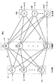
更に、上記においては、出力層43が1個の出力ユニットから成る3層ニューラルネットワーク40を用いて近似関数fを求める演算を行なう場合について説明したが、この発明によるプログラムは、図30に示す3層ニューラルネットワーク40Aを用いて近似関数fを求める演算を行なうようにしてもよい。
【0246】
図30は、この発明によるプログラムが入力値に対する出力演算値を演算する3層ニューラルネットワークの他の概念図を示す。3層ニューラルネットワーク40Aは、3層ニューラルネットワーク40の出力層43を出力層43Aに代えたものであり、その他は、3層ニューラルネットワーク40と同じである。
【0247】
出力層43Aは、出力ユニット43k(k=1〜m3)から成る。そして、出力ユニット43kは、中間ユニット42j(j=1〜m2)からそれぞれ出力Yj(j=1〜m2)を受け、その受けた出力Yj、結合重みWjk及び閾値Θkを式(4)に代入して出力演算値Z1(n),・・・,Zm3(n)(n=1〜S)を演算する。
【0248】
3層ニューラルネットワーク40Aが用いられる場合も、この発明によるプログラムは、図17及び図18に示すフローチャートに従って近似関数fを求める演算を実行する。そして、3層ニューラルネットワーク40Aを用いて近似関数fを求める演算が実行される場合、n×S個の出力値z1(n),・・・,zm1(n)が準備される。
【0249】
その他は、上述したとおりである。
更に、近似関数fを求める演算に用いる入力値及び出力値は、量子井戸に関するデータに限らず、出力値がなだらかな曲面上に存在するデータであれば、どのような種類の入力値及び出力値であってもよい。
【0250】
今回開示された実施の形態はすべての点で例示であって制限的なものではないと考えられるべきである。本発明の範囲は、上記した実施の形態の説明ではなくて特許請求の範囲によって示され、特許請求の範囲と均等の意味および範囲内でのすべての変更が含まれることが意図される。
【図面の簡単な説明】
【図1】この発明によるプログラムが近似関数を求める演算に用いる入力値と出力値とを示す図である。
【図2】入力値が2個の場合における入力値と出力値との関係を示す図である。
【図3】この発明によるプログラムが入力値に対する出力演算値を演算する3層ニューラルネットワークの概念図である。
【図4】2個の入力値を用いた場合に式(5)を用いて演算された内部状態を示す図である。
【図5】2個の入力値を用いた場合の図3に示す中間ユニットからの出力を示す図である。
【図6】2個の入力値を用いた場合に式(1)を用いて演算された内部状態を示す図である。
【図7】2個の入力値を用いた場合の図3に示す中間ユニットからの出力を示す図である。
【図8】パラメータθj及びwijの範囲を局所的特徴に相応する小さな半径にした場合における識別超球面の取り得る相対的位置関係と中間ユニット42jの出力例とを示す図である。
【図9】パラメータθj及びwijの範囲を広くした場合における識別超球面の取り得る相対的位置関係と中間ユニット42jの出力例とを示す図である。
【図10】パラメータwij(中心)が入力変数の定義域外にある小さな超球である場合における識別超球面の取り得る相対的位置関係と中間ユニット42jの出力例とを示す図である。
【図11】高次元アルゴリズムによる最適化のフローチャートである。
【図12】高次元アルゴリズムによる解の探索方法を示す概念図である。
【図13】パラメータが2個の場合におけるコスト関数のランドスケープを示す図である。
【図14】式(9)に示されるνn(qn)の概略図である。
【図15】コスト関数の局所解に捉まる度合いを高次元アルゴリズム(HA)と焼きなまし法(SA)について比較して示す図である。
【図16】コスト関数の平坦領域を通過する速さを高次元アルゴリズム(HA)と焼きなまし法(SA)について比較して示す図である。
【図17】この発明によるプログラムが入力値x1(n),・・・,xm1(n)と出力値z1(n)との関係を規定する近似関数fを求める演算を行なうフローチャートである。
【図18】図17に示すステップS2の詳細な動作を説明するためのフローチャートである。
【図19】中間ユニットの個数を1個に設定した場合の3層ニューラルネットワークの概念図である。
【図20】中間ユニットの個数を2個に設定した場合の3層ニューラルネットワークの概念図である。
【図21】二入力−一出力の3つのテスト関数の等高線を示す図である。
【図22】パーソナルコンピュータの概略ブロック図である。
【図23】量子準位演算プログラムが演算の対象とする量子井戸の概念図である。
【図24】量子準位演算プログラムを構成する各ステップを示すフローチャートである。
【図25】量子準位演算プログラムが演算の対象とする量子井戸の具体例である。
【図26】井戸ドーピングにおいて、ドーピング量を変化させたときの計算結果である。
【図27】バリアドーピングにおいて、ドーピング量を変化させたときの計算結果である。
【図28】量子準位演算プログラムを用いた計算結果と従来法による計算結果との比較を示す図である。
【図29】基底状態のエネルギー値の分割数依存性を示す図である。
【図30】この発明によるプログラムが入力値に対する出力演算値を演算する3層ニューラルネットワークの他の概念図である。
【符号の説明】
1〜6 等高線、7 曲面、10,20 集合、30 サンプルデータ、40,40A 3層ニューラルネットワーク、41 入力層、42,42A,42B中間層、43,43A 出力層、50 超平面、51,52,81 領域、60 超球面、61〜65 曲面、70 意味空間、71 解、72,82 矢印、80 高次元空間、89,105,106 曲線、90 パーソナルコンピュータ、91 CPU、92 RAM、93 ROM、94 シリアルインタフェース、95 端子、96 CD−ROMドライブ、97 ディスプレイ、98 キーボード、99 CD、100 量子井戸、101,102 バリア層、103 井戸層、104 エネルギー準位、411〜41m1 入力ユニット、421〜42m2 中間ユニット、431〜43m3 出力ユニット。[0001]
TECHNICAL FIELD OF THE INVENTION
The present invention relates to a program for causing a computer to execute an operation for obtaining an approximate function that defines a relationship between an input and an output, and a computer-readable recording medium on which the program is recorded.
[0002]
[Prior art]
Several highly accurate quantum state calculation methods considering self-interaction have been proposed. In any method, the structure parameter of the quantum well, the external electric field applied to the quantum well, and the like are used as a set of input variables. When one set of values is extracted from the set of input variables, the extracted 1 Using a set of two values as input, a computation-intensive operation such as integration of differential equations and optimization of various parameters is executed. Then, for a given input, a physically allowable energy level or wave function is calculated as an output.
[0003]
Although the prior art of the present invention has been described above based on general technical information obtained by the applicant, it should be disclosed as prior art document information before filing within the scope of the applicant's storage. The applicant has no information.
[0004]
[Problems to be solved by the invention]
However, the conventional method requires a dedicated program for calculation and sufficient calculation resources (such as a memory and a CPU (Central Processing Unit)) in order to obtain an output value for each input value. In actual nanodevice design, specific requirements are almost always imposed on the output of the above-described calculation method, such as the energy level and the wave function. That is, the energy level or wave function in the quantum well is given as a design value, and in order to realize the given energy level or wave function, the width of the well layer, the band gap of the well layer, the height of the barrier layer It is necessary to find out how to set parameters such as the width of the barrier layer, the band gap of the barrier layer, and the doping amount of the dopant in the well layer or the barrier layer.
[0005]
In this case, if the conventional method described above is used, it is necessary to search for a system that satisfies the condition while changing the input value by trial and error, but for that purpose, an enormous amount of calculation is required, and the design of nanodevices is required. It is not efficient to perform the operation every time.
[0006]
Therefore, the present invention has been made to solve such a problem, and an object of the present invention is to provide a program for causing a computer to execute an operation for obtaining an approximate function that defines a relationship between an input and an output. is there.
[0007]
Another object of the present invention is to provide a computer-readable recording medium on which a program for causing a computer to execute an operation for obtaining an approximate function that defines a relationship between an input and an output is recorded.
[0008]
Means for Solving the Problems and Effects of the Invention
According to the present invention, m (m is a natural number) input values and n (n is a natural number) output values are used, and m (m is a natural number) sample data and m (m is a natural number) sample data are used. A program for causing a computer to execute an operation for obtaining an approximate function that defines a relationship with n outputs includes: a first step of receiving m × S input values and n × S output values; The parameter value of the discriminating hypersphere among all parameters of the three-layer neural network of the hypersphere discrimination type that calculates n output calculation values for the input values is changed in a search range wider than a normal search range. Then, n × S output operation values for m × S input values are calculated by hypersphere identification type operation, and an approximate function is obtained using the calculated n × S output operation values. The second step is to optimize the values of all parameters The second step is to set a high-dimensional space higher than the number of dimensions defined by the number of all parameters, and the values of all parameters in the set high-dimensional space are other than optimal values. Is a program to be executed by a computer for optimizing all parameters by a high-dimensional algorithm which is expected to pass through an area quickly and easily enter an area where all parameter values are optimal.
[0009]
Preferably, in the second step, the number of intermediate units included in the three-layer neural network and performing the operation of the hypersphere identification type is set to an initial value, and n × S output operation values are calculated, Optimize all parameters.
[0010]
Preferably, the second step is a first sub-step of setting all parameters to initial values and calculating n × S output calculation values by a hypersphere identification type calculation, and the calculated n × S calculation values A second sub-step of calculating a cost function value for evaluating the output calculation value of the above, and comparing the calculated cost function value with a predetermined value; and when the cost function value is equal to or less than the predetermined value, the cost function value is obtained. A third sub-step of optimizing the values of all the parameters of the above, and, when the cost function value is larger than a predetermined value, calculating all parameters for reducing the cost function value by a high-dimensional algorithm in a wide search range. A fourth sub-step and a fifth sub-step in which the first sub-step is executed using all the parameters calculated in the fourth sub-step, and thereafter the second to fourth sub-steps are executed. When the cost function value obtained when the first and fifth sub-steps are repeatedly executed up to a specified number of times is larger than a predetermined value, the number of intermediate units is increased and the first to fifth sub-steps are executed. And a sixth sub-step.
[0011]
Preferably, the number of intermediate units is increased one by one.
Preferably, the initial value of the number of intermediate units is one.
[0012]
Preferably, in the second step, the number of all parameters is set to an initial value, n × S output operation values are calculated, and optimization of all parameters is performed.
[0013]
Preferably, the second step is a first sub-step of setting all parameters to initial values and calculating n × S output calculation values by a hypersphere identification type calculation, and the calculated n × S calculation values A second sub-step of calculating a cost function value for evaluating the output calculation value of the above, and comparing the calculated cost function value with a predetermined value; and when the cost function value is equal to or less than the predetermined value, the cost function value is obtained. A third sub-step of optimizing the values of all the parameters of the above, and, when the cost function value is larger than a predetermined value, calculating all parameters for reducing the cost function value by a high-dimensional algorithm in a wide search range. A fourth sub-step and a fifth sub-step in which the first sub-step is executed using all the parameters calculated in the fourth sub-step, and thereafter the second to fourth sub-steps are executed. When the cost function value obtained by repeatedly executing the first to fifth sub-steps up to a specified number of times is larger than a predetermined value, the number of all parameters is increased and the first to fifth sub-steps are executed. And a sixth sub-step.
[0014]
Preferably, all parameters are incremented by a predetermined number. Then, when the number of all parameters is increased, the first to fifth sub-steps of the program are executed by fixing the values of a predetermined number of parameters before the number of all parameters is increased.
[0015]
Preferably, when a predetermined number of parameters before the number of all parameters is increased is set as a first parameter, and the increased predetermined number of parameters is set as a second parameter, the fourth sub-step includes: The parameters are fixed, the second parameter is changed in a wide search range, and all parameters for reducing the cost function value are calculated by a high-dimensional algorithm.
[0016]
Preferably, the second sub-step calculates, as a cost function value, an average of the sum of square errors of the received n × S output values and the calculated n × S output calculation values.
[0017]
Preferably, the n × S output values are approximated by a combination of Gaussian-like distributions.
[0018]
Preferably, the m × S input values and the n × S output values are data calculated by a computer.
[0019]
Preferably, the m × S input values and the n × S output values are data calculated by a quantum level calculation program for calculating quantum levels of particles confined in the microstructure. Then, the quantum level calculation program calculates an initial wave function based on the linear Schrodinger equation, and gives the calculated initial wave function as a numerical sequence composed of a plurality of discretized components; Using the first wave function having a plurality of discretized components and the Hamiltonian including a nonlinear term in consideration of the interaction between particles, the first wave function is normalized by the number of particles present in the microstructure, and the energy of the entire system is A step B of calculating a cost function indicating the following, a step C of calculating a final wave function that minimizes the total energy of the system using the calculated cost function, and a step C of calculating the final wave function and the Hamiltonian. Calculating the energy of the state represented by the final wave function.
[0020]
Preferably, the high-dimensional algorithm comprises a step of defining a space of all parameters that appear in the problem to be solved and to be optimized as a semantic space, a step of defining a new space by a conjugate parameter conjugate to all the parameters, Defining a high-dimensional space by adding a new space to, a step of setting a problem in the high-dimensional space, and quickly passing through a region where the values of all parameters are other than optimal values, and the values of all parameters are optimal values. Performing an autonomous motion expected to easily enter a certain area in a high-dimensional space to detect the optimal values of all parameters.
Further, according to the present invention, a computer-readable recording medium storing a program for causing a computer to execute an operation for obtaining an approximation function includes a program according to any one of
[0021]
The program according to the present invention calculates an output operation value for an input value by using a three-layer neural network by changing a hypersphere parameter when performing a hypersphere identification type operation in a range wider than a normal search range. Then, the program according to the present invention optimizes parameters using a high-dimensional algorithm so that a cost function for evaluating the calculated output operation value is equal to or less than a predetermined value, and performs an approximation that defines a relationship between an input value and an output value. Operate a function.
[0022]
Therefore, according to the present invention, an approximate function that can easily obtain an output value with respect to an input value can be obtained.
[0023]
Further, in the present invention, when calculating the output calculation value, the program changes the search range of the parameter in a range wider than the normal search range, and performs the calculation of the hypersphere identification type.
[0024]
Therefore, according to the present invention, both the local feature and the global feature can be efficiently reflected in the output operation value.
[0025]
Furthermore, in the present invention, the program optimizes the parameters using a high-dimensional algorithm that performs an autonomous motion in a high-dimensional space higher than the number of dimensions set by the number of parameters of the three-layer neural network. The autonomous motion refers to a motion that quickly passes through a region where a value other than the optimum value of the parameter exists and easily enters a region where the optimum value exists.
[0026]
Therefore, according to the present invention, it is difficult to catch the local solution of the cost function for evaluating the output operation value, and the parameter can be optimized by quickly passing through the flat region of the cost function.
[0027]
In particular, if the search range of the parameter is widened when performing the operation of the hypersphere identification type, the flat region of the cost function increases, but the high-dimensional algorithm has a feature that the optimal solution is obtained by quickly passing through the flat region. As a result, both the local feature and the global feature can be reflected in the output operation value, and the parameters can be optimized quickly.
[0028]
BEST MODE FOR CARRYING OUT THE INVENTION
Embodiments of the present invention will be described in detail with reference to the drawings. In the drawings, the same or corresponding portions have the same reference characters allotted, and description thereof will not be repeated.
[0029]
FIG. 1 shows input values and output values used by a program according to the present invention for calculating an approximate function. The
[0030]
The output value z (1) is a set of input values (x1(1), ..., xm1(1)), the output value z (2) is the set of input values (x1(2), ..., xm1(2)), and similarly, the output value z (M) is similarly set to the set of input values (x1(M), ..., xm1(M)). Also, a set of input values (x1(1), ..., xm1(1)), (x1(2), ..., xm1(2)),..., (X1(S), ..., xm1(S)),..., (X1(M), ..., xm1(M)) and output values z (1), z (2),..., Z (S),. It is.
[0031]
The method for obtaining the set of these input values and the output value will be described later.
From the
[0032]
In this way, the
[0033]
The program according to the present invention uses the
[0034]
FIG. 2 shows a relationship between an input value and an output value when there are two input variables. FIG. 2A shows a set x of two input values.1(N), x2(N) and a set x of two input values1(N), x2The plot points of (n) and the contour lines of the function f are shown. In FIG. 2A, a black circle indicates a set x of two input values.1(N), x2A set x of two input values when each of (n) changes in the range [0, 1]1(N), x2The plot point of (n) is shown, and the solid line shows the contour of the function f. FIG. 2B is a three-dimensional expression of the function f.
[0035]
In this case, the
[0036]
The
[0037]
In the present invention, a “smooth curved surface” refers to a curved surface represented by a combination of Gaussian-like distributions.
[0038]
FIG. 3 is a conceptual diagram of a three-layer neural network in which a program according to the present invention calculates an output operation value Z (n) for an input value. The three-layer
[0039]
The
[0040]
The input unit 41i has an input value x input to the i-th unit of the input layer 41.i(N) and the received input value xi(N) is transmitted to each of the m2 intermediate units 42j.
[0041]
The
[0042]
(Equation 1)
That is, the intermediate unit 42j performs an operation of the hypersphere identification type. The reason why the intermediate unit 42j performs the operation of the hypersphere identification type will be described later.
[0044]
Then, the intermediate unit 42j calculates the calculated internal state y.jInto equation (2) and output YjIs calculated.
[0045]
(Equation 2)
That is, the intermediate unit 42j outputs the output Y using the sigmoid function.jIs calculated. In equation (2), TjIs a parameter for adjusting the slope of the transition region of the sigmoid function. In this embodiment, in order to prevent the exponential function included in the denominator on the right side of Expression (2) from diverging numerically, TjIs defined by equation (3).
[0047]
(Equation 3)
In equation (3), τjRepresents the slope of the output function of the intermediate unit 42j.
The intermediate unit 42j outputs the output YjIs calculated, the calculated output YjTo the
[0049]
The
[0050]
(Equation 4)
In equation (4), WjIs the connection weight with the j-th intermediate unit 42j, and Θ is the threshold value of the
[0052]
In the present invention, the number of intermediate units is initially set to one, and is increased by one in accordance with the calculation result of obtaining the approximate function f using the set one intermediate unit. . Therefore, the
[0053]
Thus, the three-layer
[0054]
The intermediate unit 42j is in the internal state yjThe reason for performing the operation of the hypersphere discrimination type in accordance with equation (1) in order to obtain the following equation will be described. In general, the internal state yjThe input value x represented by equation (5) to determinei(N) and the parameter w of the combinationijIs often used.
[0055]
(Equation 5)
In this case, the equation y of the identification surfacej= 0 specifies one hyperplane. Examples are shown in FIGS. FIG. 4 shows a set x of two input values.1(N), x2Internal state y calculated using equation (5) when (n) is usedjIs shown. FIG. 5 shows a set x of two input values.1(N), x2Output Y from intermediate unit when (n) is usedjIs shown.
[0057]
As shown in FIG. 4, the equation y of the identification surfacej= 0 designates one
[0058]
Using the equation (5), the internal state yjIs referred to as hyperplane identification type operation. Then, when the operation of the hyperplane identification type is performed, as described above, the global feature can be expressed, but the local feature cannot be expressed by one intermediate unit. Representing local features requires a number of intermediate units.
[0059]
On the other hand, using the equation (1), the internal state yjIs calculated, the equation y of the identification surfacej= 0 specifies one hypersphere. Examples are shown in FIGS. FIG. 6 shows a set x of two input values.1(N), x2Internal state y calculated using equation (1) when (n) is usedjIs shown. FIG. 7 shows a set x of two input values.1(N), x2Output Y from intermediate unit 42j when (n) is usedjIs shown.
[0060]
As shown in FIG.j= 0 designates one
[0061]
As described above, the internal state y is calculated by the operation of the hyperplane identification type.jIs obtained, global features can be expressed, but local features cannot be expressed. On the other hand, the internal state yj, Local features can be expressed, but global features cannot be expressed.
[0062]
Therefore, ideally, an intermediate unit that is advantageous for expressing local features and an intermediate unit that is advantageous for expressing global features should be aligned, but it is unknown how many should be aligned. If the operation of the hyperplane identification type and the operation of the hypersphere identification type are performed in a mixed manner, the amount of calculation increases.
[0063]
Therefore, in the present invention, the operation of the hyperspherical identification type which is advantageous for the expression of the local feature is adopted, and the intermediate unit 42j has the internal state yjAnd output Yj(Θj, Wij, Τj) Is changed over a wider range than the normal search range to express global features.
[0064]
A set x of two input values1(N), x2When (n) is used, the equation y of the identification surfacej= 0 from Equation (1), the parameter wijAnd the parameter θjSpecify a circle whose radius is. Parameter θjAnd wijThe change of the function f when the range is changed will be described.
[0065]
FIG. 8 shows the parameter θjAnd wijShows a relative positional relationship of the identification hypersphere and an output example of the intermediate unit 42j in the case where the range is set to a small radius corresponding to the local feature. FIG. 9 shows the parameter θjAnd wijShows the relative positional relationship of the identification hypersphere and the output example of the intermediate unit 42j when the range is widened. FIG. 10 shows the parameter wij(Center) is the input variable x1, X2Fig. 7 shows possible relative positional relationships of the discriminating hypersphere and an output example of the intermediate unit 42j in the case of a small hypersphere existing outside the defined range.
[0066]
Parameter (w1j, W2j) (Center) is the input variable x1, X2Within the domain ([0,1]2) And the parameter θjWhen the possible range of (radius) is as small as [0, 0.5] (see FIG. 8A), the intermediate unit 42j outputs the output Y represented by the
[0067]
The
[0068]
Thus, the parameter (w1j, W2j) (Center) is the input variable x1, X2And set the parameter θjIf (radius) is set to a small value, the intermediate unit 42j outputs the output Y represented by the
[0069]
Parameter (w1j, W2j) (Center) is the input variable x1, X2Outside the domain of [(-0.2, 1.2]2) And the parameter θjWhen the possible range of (radius) is as large as [0, 1.5] (see FIG. 9A), the intermediate unit 42j outputs the output Y represented by the
[0070]
The
[0071]
The curved surfaces 63 and 64 are similar to the curved surface shown in FIG. Therefore, the parameter (w1j, W2j) (Center) is the input variable x1, X2Outside the defined range, and the parameter θjIf (radius) is set to a large value, the intermediate unit 42j outputs the output Y represented by the
[0072]
Parameter (w1j, W2j) (Center) is the input variable x1, X2Outside the domain of the parameter θjWhen the (radius) is small (see FIG. 10A), the intermediate unit 42j outputs the output Y represented by the curved surface 65.jIs output (see FIG. 10B).
[0073]
In this case, the intermediate unit 42j outputs a
[0074]
As described above, the parameter θj, WijAnd Tj(That is, τj), The intermediate unit 42j outputs the output Y reflecting the local feature in the operation of the hypersphere identification type.j(See FIG. 8) and output Y reflecting global featuresj(See FIG. 9). Even if the local feature and the global feature are reflected by the operation of the hypersphere identification type, the number of parameters of the intermediate unit 42j does not increase. Accordingly, in the present invention, the intermediate unit 42jj, WijAnd Tj(That is, τj) Is changed to a range wider than the range for performing the operation of the normal hypersphere identification type, and the operation of the hypersphere identification type is performed, and the output YjWas output. This is the reason that the intermediate unit 42j performs the operation of the hypersphere identification type.
[0075]
The “normal search range” means that only the local features are output by the operation of the hypersphere identification type.jParameter θ to reflectj, WijAnd Tj(That is, τj).
[0076]
Output Y from intermediate unit 42jjIs input to the
[0077]
Output operation value Z1When (n) is calculated, the output value z included in the
[0078]
(Equation 6)
The average V of the sum of squared errors (wij, Θj, Τj, Wj, Θ) are output operation values Z calculated by the three-layer neural network 40.1(N) is the actual output value z1(N) is an index indicating a degree close to (n).1This is a cost function for evaluating (n).
[0080]
The program according to the present invention has a parameter wij, Θj, Τj, Wj, ((The parameter w of the intermediate unit 42j)ij, Θj, ΤjIs changed in a range wider than the range reflecting the local feature), and the output operation value Z1(N) and the output operation value Z1Cost function V (w) calculated by substituting (n) into equation (6)ij, Θj, Τj, Wj, Θ) such that the parameter wij, Θj, Τj, Wj, Θ is optimized. In this case, the program according to the present invention first sets the number of intermediate units 42j to one (j = 1), and finally calculates the cost function V (w using the one set
[0081]
This parameter wij, Θj, Τj, Wj, Θ are optimized, the input value x1(N), ..., xm1(N) and output value z1(N) Since the approximate function f that defines the relationship with (n = 1 to S) is determined, the parameter wij, Θj, Τj, Wj, Θ corresponds to performing an operation for obtaining the approximate function f.
[0082]
As described above, the intermediate unit 42j includes the parameter wij, Θj, ΤjIs changed in a range wider than the range reflecting the local feature, and the operation of the hypersphere identification type is performed.ij, Θj, ΤjIs changed over a wide range, the cost function V (wij, Θj, Τj, Wj, Θ) will increase the wide flat area. As shown in FIG. 10A, the center wijIs outside the defined range of the input value, and the radius θjIs smaller than the output Y of the intermediate unit 42j.jIs substantially zero in the entire domain and the output operation value Z which is the final output1It hardly contributes to (n). Therefore, in a region corresponding to such a situation in the parameter space, the cost function V (wij, Θj, Τj, Wj, Θ) becomes flat.
[0083]
wij, Θj, Τj, Wj, Θ, an algorithm such as an error back-propagation algorithm (BP) or an annealing method (SA: Simulated Annealing) which is often used when optimizing parameters such as Very inefficient against A method of adding a penalty term to the cost function in order to avoid the appearance of a wide flat area is also conceivable, but this method distorts the original cost function and increases the amount of calculation required for evaluating the cost function.
[0084]
Therefore, in the present invention, a high-dimensional algorithm, which is an effective optimization method for a cost function including a wide flat region and a plurality of local solutions which are always problematic in learning a neural network, is adopted.
[0085]
The optimization of the parameters by the high-dimensional algorithm will be described. FIG. 11 shows a flowchart of optimization by a high-dimensional algorithm. The space of all variables q to be optimized appearing in the problem to be solved is defined as a semantic space (step A). Then, a variable p conjugate with the variable q is artificially introduced to define a new space for the variable p (step B). Then, the space of the variable p is added to the semantic space, and a space obtained by increasing the dimension of the semantic space is defined as a high-dimensional space (step C).
[0086]
Then, a problem is set in a high-dimensional space of variables q and p (step D). Finally, in a high-dimensional space, an optimal solution is searched by autonomous motion, and an optimal solution that minimizes the cost function is detected (step E). Here, the autonomous motion refers to a motion that quickly passes through a region where a solution does not exist and easily enters a region where a solution exists.
[0087]
As described above, the high-dimensional algorithm increases the dimension of the semantic space of the variable q to be optimized, and detects an optimal solution by performing an autonomous motion in the increased high-dimensional space.
[0088]
FIG. 12 is a conceptual diagram illustrating a solution search method using a high-dimensional algorithm. FIG. 13 shows a landscape of the cost function when the number of parameters is two (k1, k2). In the landscape shown in FIG. 13, there are many peaks and valleys, and the solution corresponds to the lowest point (minimum value) of all valleys. Therefore, in order to find a solution, it is necessary to reach the lowest valley through many complicated peaks and valleys.
[0089]
That is, as shown in FIG. 12, in order to reach the
[0090]
Therefore, a high-
[0091]
Thus, it can be clearly understood from the following example that the object can be easily searched if the space to be searched is increased in dimension. For example, consider the case of searching for a hexagonal pencil with a long cut. When you look at this pencil from the front, you can only see a small hexagonal cross section, but if you look away, you can see the length of the cut. If this "length" is considered as a dimension, it can be easily understood that by increasing the dimension from the
[0092]
The high-dimensional algorithm increases the space to be searched in this way and searches for a solution in the higher-dimensional space.As a result, the high-dimensional algorithm is less likely to be caught by the local solution of the cost function, and the flat region of the cost function is reduced. It can pass quickly and can easily find a global solution.
[0093]
Output operation value Z calculated by three-layer neural network 401(N) is the actual output value z1Parameter w using a high-dimensional algorithm so as to approach (n)ij, Θj, Τj, Wj, Θ, the program according to the present invention uses Hamiltonian H (q, p) which is a function of variables q, p in high
[0094]
In the case of the problem of obtaining the approximate function of the present invention, the variable q to be optimized by the high-dimensional algorithm is q = wij, Θj, Τj, Wj, Θ (see step A in FIG. 11). And this variable q = wij, Θj, Τj, Wj, Θ correspond to the position of the moving object. The potential energy V (q) is a variable q = wij, Θj, Τj, Wj, Θ.
[0095]
Next, a variable p conjugate to the variable q is artificially introduced, and a new space formed by the variable p is defined (see step B in FIG. 11). The new space added to the semantic space is defined as a high-dimensional space (see step C in FIG. 11). The variable p corresponds to the velocity of the moving object as described above, and defines a function corresponding to the kinetic energy T (p) which is a function of the variable p in the same manner as the moving dynamic system (see step D in FIG. 11). ).
[0096]
Thereafter, a function H (q, p) in a high-dimensional space obtained by adding a function T (p) in a new space to a function V (q) in the semantic space to increase the dimension of the semantic space is defined by variables q and p ( (See step D in FIG. 11).
[0097]
In a Hamiltonian dynamical system, the position of a moving object at an arbitrary time t is determined by a motion equation derived from the Hamiltonian H (q, p), and therefore the same applies to a high-dimensional algorithm.
[0098]
Finally, detecting an optimal solution by autonomous motion in a high-dimensional space is equivalent to finding an optimized variable q by solving a motion equation derived from the Hamiltonian H (q, p) (FIG. 11). Step E).
[0099]
The potential energy V (q) is represented by equation (7).
[0100]
(Equation 7)
That is, the potential energy V (q) is represented by the cost function VC(Q) and constraint potential VL(Q). This constraint potential VL(Q) is a parameter q = wij, Θj, Τj, Wj, Θ are limited. And the constrained potential VL(Q) is represented by equation (8).
[0102]
(Equation 8)
In the equation (8), c is a parameter for controlling the strength of the constraint, and in this embodiment, c = 1 is set. Also, ν in equation (8)n(Qn) Is represented by equation (9).
[0104]
(Equation 9)
In equation (9), θ (u) represents a step function, and u = an-QnOr qn-BnWhen> 0, θ (u) = 1 and u = an-QnOr qn-BnWhen <0, θ (u) = 0.
[0106]
That is, νn(Qn) Is represented by the
[0107]
Further, the kinetic energy T (p) is represented by Expression (10), and the Hamiltonian H (q, p) is represented by Expression (11).
[0108]
(Equation 10)
(Equation 11)
As a result, the equation of motion describing the motion of the system is represented by equation (12).
[0111]
(Equation 12)
Further, the cost function V appearing on the right side of the lower expression of Expression (12)C(Q) and the function V indicating the constrained potentialLParameter q = w of (q)ij, Θj, Τj, Wj, Θ are shown in equations (13) and (14), respectively.
[0113]
(Equation 13)
[Equation 14]
Starting from a randomly selected initial value (q (0), p (0)), a set of 2N first-order differential equations of equation (12) is obtained by a Verlet method or a Runge-Kutta method. , The orbit (q (t), p (t)) of the system is obtained. Then, the cost function V along the trajectory q (t) for a sufficient timeCBy monitoring (q (t)), the parameter q = wij, Θj, Τj, Wj, Θ can be found.
[0116]
The motion system described by the motion equation shown in Expression (12) is a dynamic system having mixing properties and a constant total energy E. In this case, the system is expected to move around with equal probability on an equal energy surface that satisfies H (q, p) = E in the phase space (the principle of equal weight). Based on this isobaric principle, the expected value δ (q) of the time the system stays in the microvolume q + dq near the position q is expressed by equation (15) (K. Shinjo) And T. Sasada, "Hamiltonian Systems with Many Degrees of Freedom: Asymmetric Motion and Intensity of Motion in a Phase of Space in the Phase of Space in the Phase of Space in the Phase Space" Physical Review E54, pp4685-4700, 1996 ).
[0117]
[Equation 15]
From Expression (15), when the degree of freedom N is 3 or more, the expected value of the stay time is low in the region having a high potential value, and the expected value of the stay time is high in the region having a low potential value. Becomes more remarkable as the degree of freedom N increases.
[0119]
Therefore, the high-dimensional algorithm takes the analogy of the dynamical system of the Hamiltonian H (q, p) having such characteristics and searches for the optimal solution, so that it is hard to be caught by the local solution of the cost function described above, and It has the feature that it quickly passes through a flat area of the cost function.
[0120]
The features of this high-dimensional algorithm will be described conceptually.
FIG. 15 shows the degree of the localization of the cost function captured by the high-dimensional algorithm (HA) and the annealing method (SA) in comparison. FIG. 15A shows the case of the high-dimensional algorithm (HA), and FIG. 15B shows the case of the annealing method (SA). 15A and 15B, the horizontal axis represents the variable q to be optimized, and the vertical axis represents the cost function V (q).
[0121]
FIG. 16 shows the speed of the cost function passing through the flat region in comparison with the high-dimensional algorithm (HA) and the annealing method (SA). FIG. 16A shows the case of the high-dimensional algorithm (HA), and FIG. 16B shows the case of the annealing method (SA). 16A and 16B, the horizontal axis represents the variable q to be optimized, and the vertical axis represents the cost function V (q).
[0122]
As shown in FIG. 15, in the case of the high-dimensional algorithm (HA), the kinetic energy E plays a role of getting out of the valley (local solution) of the cost function V (q). , The value becomes large at a position where the function value of the cost function is small. In other words, the kinetic energy E increases when entering the local solution. Therefore, the high-dimensional algorithm (HA) is hardly caught by a local solution (see FIG. 15A). On the other hand, in the case of the annealing method (SA), the movement can escape from the local solution by having a positive absolute temperature, but this absolute temperature is position-independent. Therefore, if the absolute temperature is lower than the peak of the cost function, it is difficult to escape from the local solution. As a result, the annealing method (SA) is easily captured by the local solution of the cost function (see FIG. 15B).
[0123]
Also, as shown in FIG. 16, in the case of the high-dimensional algorithm (HA), since the robot moves in one direction by linear motion at a constant velocity, it passes through the flat region of the cost function V (q) quickly (( a)). On the other hand, in the case of the annealing method (SA), since it moves by a random walk (moves randomly in each step in the right and left directions on the paper), it cannot easily pass through the flat area of the cost function V (q) (see FIG. 16 (b)).
[0124]
As described above, the high-dimensional algorithm has a feature that it is hard to be caught by the local solution of the cost function and can pass through the flat region quickly. As a result, an optimal solution can be reached with a small amount of calculation.
[0125]
FIG. 17 shows a program according to the present invention in which a set of input values x1(N), ..., xm1(N) and
[0126]
That is, the parameter w of the intermediate unit 42j of the three-layer
[0127]
FIG. 18 shows a flowchart for explaining the detailed operation of step S2 shown in FIG. After step S1 shown in FIG. 17, the parameter w of the three-layer
[0128]
Then, S output operation values Z1(1), ..., Z1A cost function value for evaluating (S) is calculated (step S22). Thereafter, it is determined whether or not the cost function value is equal to or smaller than the predetermined value ε (step S23). When the cost function value is equal to or smaller than the predetermined value ε, a series of operations ends.
[0129]
On the other hand, when it is determined in step S23 that the cost function value is not equal to or smaller than the predetermined value ε, it is determined whether the number of calculations is equal to or smaller than a specified number (step S24). Then, when the number of calculations is equal to or less than the specified number, a parameter for reducing the cost function value is calculated over a wide search range by a high-dimensional algorithm (step S25).
[0130]
That is, the cost function value and the constraint condition calculated in step S22 are converted into the parameter w by the equations (13) and (14).ij, Θj, Τj, Wj, Θ, and the value of the parameter w to be next taken by equation (12).ij, Θj, Τj, Wj, Θ are calculated. Then, the calculated value is used as the parameter w used in the calculation in step S21.ij, Θj, Τj, Wj, Θ.
[0131]
Thus, after step S25, steps S21 to S24 are repeatedly executed.
[0132]
On the other hand, when it is determined in step S24 that the number of calculations is not less than or equal to the prescribed number, the parameter with the smallest cost function value in a series of iterations is fixed to the optimum value of the intermediate unit, and the three-layer
[0133]
As described above, according to the program of the present invention, the number of the intermediate units 42j is initially set to one, and the set one
[0134]
When step S2 shown in FIG. 17 is performed first, the number of the intermediate units 42j of the
[0135]
In this case, the
[0136]
The
[0137]
Cost function VC(Q) is the input value x1(N), ..., xm1(N) (n = 1 to S) and output value z1The calculation for obtaining the approximate function f defining the relationship with (n) is represented by Expression (6). Therefore, the calculated output operation value Z11(N) and the actual output value z1(N) is substituted into equation (6), and the cost function V ((wi1, Θ1, Τ1, W1, Θ)11) Cost function value V11Is calculated (see step S22 in FIG. 18). Note that the cost function value V11The meaning of the subscript {11} of the parameter (wi1, Θ1, Τ1, W1, Θ)11And output operation value Z11This has the same meaning as the subscript (n).
[0138]
And the cost function value V11Is not less than the predetermined value ε, the cost function value V11Cost function value V smaller than12(Wi1, Θ1, Τ1, W1, Θ)12Is obtained by a high-dimensional algorithm (see step S25 in FIG. 18). Then, the parameter (wi1, Θ1, Τ1, W1, Θ)12And S output operation values Z12(N) is calculated (see step S21 in FIG. 18), and the cost function value V is calculated by equation (6).12Is calculated (see step S22 in FIG. 18).
[0139]
And the cost function value V12Is determined to be less than or equal to a predetermined value ε (step S23 in FIG. 18), and the cost function value V12Is not less than or equal to the predetermined value ε, the cost function value V smaller than the already calculated minimum cost function value1h(H: natural number of h ≦ k, k: specified number of times)i1, Θ1, Τ1, W1, Θ)1hIs calculated (see step S25 in FIG. 18).
[0140]
As described above, when the number of calculations is equal to or less than the specified number k, the cost function value V1h(H is a natural number less than or equal to k)i1, Θ1, Τ1, W1, Θ)1hIs calculated, and the calculated parameter (wi1, Θ1, Τ1, W1, Θ)1hAnd a new cost function value V1hIs calculated, and this is repeated one after another. That is, the parameter (wi1, Θ1, Τ1, W1, Θ) while monitoring the corresponding cost function value, searching for the smallest cost function value and the parameter corresponding to the smallest cost function value.
[0141]
Then, when the number of calculations reaches the specified number, the number of intermediate units 42j is increased by one and set to two (see step S26 in FIG. 18).
[0142]
FIG. 20 is a conceptual diagram of the three-layer
[0143]
In this case, the
[0144]
Further, the
[0145]
The
[0146]
And the output operation value Z21Using (n), the cost function value V21Is calculated, and the same calculation as when only the
[0147]
As described above, when the number of the intermediate units 42j is set to a certain value, the cost function value for evaluating the output operation value Z (n) calculated using the set number of the intermediate units 42j is optimally reduced. To determine the value, a new parameter (wij, Θj, Τj, Wj, Θ) are calculated one after another by a high-dimensional algorithm. If the cost function value does not become less than or equal to the predetermined value ε even after performing the calculation of the new parameter up to the specified number of times, the new parameter (wij, Θj, Τj, Wj, Θ) are calculated one after another by a high-dimensional algorithm.
[0148]
Therefore, the program according to the present invention increases the number of intermediate units 42j of the three-layer
[0149]
In the above description, the number of intermediate units 42j is initially set to “1”. However, the present invention is not limited to this, and may be initially set to a plurality. That is, in the present invention, the number of intermediate units 42j may be initially set to one or more initial values.
[0150]
The parameters of the three-layer neural network 40 (wij, Θj, Τj, Wj, Θ) increase by (m1 + 3) as the number of intermediate units 42j increases. For example, when the number of intermediate units 42j increases from one to two, the overall parameters are (wi1, Θ1, Τ1, W1, Θ) to (wi1, Θ1, Τ1, W1; Wi2, Θ2, Τ2, W2, Θ) by (m1 + 3). Therefore, the number of intermediate units 42j is increased by one and the parameter (wij, Θj, Τj, Wj, Θ) is to increase the number of parameters by a predetermined number and increase the number of parameters (wij, Θj, Τj, Wj, Θ) is equivalent to optimizing. Then, among the predetermined number of parameters before the number of parameters is increased, the parameter (wi1, Θ1, Τ1, W1) Is fixed and the increased parameter (wi2, Θ2, Τ2, W2) And the parameter Θ, the parameter (wi2, Θ2, Τ2) In a wide search range to change the output operation value Z1(N) is calculated. In this case, in step S2 shown in FIG. 17, the number of parameters is set to a predetermined initial value to optimize the parameters.
[0151]
Therefore, the program according to the present invention is characterized in that the number of parameters of the three-layer neural network is increased by a predetermined number to optimize the parameters.
[0152]
The effect of the three-layer
[0153]
FIG. 21 shows the contours of three test functions with two inputs and one output. FIG. 21A shows that the test function z is expressed as z = −0.76x1+ 0.19x2The contour line when +0.78 is set is shown. FIG. 21B shows that the test function z is expressed as z = sin (πx1) · Sin (πx2) Indicates contour lines. FIG. 21C shows that the test function z is expressed as z = 0.5exp {−5 (x1-0.2)2-5 (x2-0.2)2{+ 0.9exp} -5 (x1-0.8)2-10 (x2-0.6)2Shows the contour line when}. 21A, 21B, and 21C, the horizontal axis and the vertical axis represent the input variable x.1, X2Represents
[0154]
Each learning condition is as follows.
[0155]
For problem (i), the following results were obtained:
<1> Hyperplane identification network
Number of acquired intermediate units = 1
Average number of times of learning ≒ 11,507 times
<2> Hypersphere identification network
Number of acquired intermediate units = 1
Average learning times: 64,103 times
As shown in FIG. 21A, the contours of this test function are linear, which is a clear advantage for hyperplane identification networks. However, even in the hypersphere discrimination network, since a relatively strict required accuracy (ε ≦ 0.003) is achieved by one intermediate unit, by expanding the parameter search range, if only local features are used, However, it can be understood that the global characteristics can be reflected, and the mapping ability is enhanced.
[0156]
On the other hand, the hypersphere discrimination network has about six times the average number of times of learning as the hyperplane discrimination network. This is due to the fact that the parameter search range is widened, but despite the clearly disadvantageous case, the increase is at most about 6 times.
[0157]
Next, the result of the problem (ii) will be described.
<1> Hyperplane identification network
Number of acquired intermediate units = 8
Average number of times of learning 393,829 times
<2> Hypersphere identification network
Number of acquired intermediate units = 1
Average number of learnings = 12,045 times
As shown in FIG. 21 (b), the contour of this test function is a closed curve, which is a case clearly advantageous for the hypersphere discrimination network. For the hyperplane discrimination network, if the required accuracy was raised to ε ≦ 0.03, convergence of learning became difficult rapidly, so ε ≦ 0.05. The required number of intermediate units is a result of eight hyperplane discrimination networks and one hypersphere discrimination network, which shows that the mapping ability of the hypersphere discrimination network is superior to each stage. .
[0158]
As for the average number of times of learning, the hyperplane identification network requiring eight times the number of intermediate units (the number of parameters) is about 33 times as large, which indicates that the hyperplane identification network is inefficient for expressing local features.
[0159]
Finally, the results of problem (iii) are shown.
<1> Hyperplane identification network
Number of acquired intermediate units = 6
Average number of learnings: 264,706
<2> Hypersphere identification network
Number of acquired intermediate units = 2
Average number of learning ≒ 2,665 times
As shown in FIG. 21C, this test function has an asymmetrical closed contour and is an example likely to be a practical application problem. Since it was difficult for the hyperplane identification network to achieve the required accuracy ε ≦ 0.01, ε ≦ 0.03 was set.
[0160]
The number of intermediate units is two for the hypersphere identification network and six for the hyperplane identification network. As a result, it can be seen that also in this case, the hyperspherical identification network has higher mapping ability. The average number of times of learning is also nearly 100 times greater in the hyperplane identification network than in the hypersphere identification network.
[0161]
As described above, a method of learning a hypersphere identification network in which a parameter search range is appropriately expanded by a high-dimensional algorithm generally has a high mapping ability capable of achieving required accuracy with a smaller number of parameters than in the case of a hyperplane identification network. It was confirmed that the learning performance was good.
[0162]
A program including steps S1 and S2 shown in FIG. 17 and steps S21 to S26 shown in FIG. 18 is executed by the personal computer shown in FIG. FIG. 22 is a schematic block diagram of a personal computer. The
[0163]
[0164]
The
[0165]
The terminal 95 is a terminal for connecting the
[0166]
[0167]
The program according to the present invention is read from the
[0168]
Thus, the user can execute the program according to the present invention by the
[0169]
As described above, the program according to the present invention uses the input value x1(N), ..., xm1(N) (n = 1 to S) and output value z1When performing an operation for obtaining an approximate function f that defines the relationship with (n), the input value (x1(1), ..., xm1(1)), (x1(2), ..., xm1(2)),..., (X1(S), ..., xm1(S)),..., (X1(M), ..., xm1(M)) and output values (z (1), z (2),..., Z (S),..., Z (M)) included in the
[0170]
Therefore, the width d of the well layerw1, The electron density n of the well layerw1, Barrier layer height Wd2And the width d of the barrier layerbInput value (x1(1), ..., xm1(1)), (x1(2), ..., xm1(2)),..., (X1(S), ..., xm1(S)),..., (X1(M), ..., xm1(M)) and the energy level Ew1, Z (S),..., Z (M)) will be described.
[0171]
[How to get sample data]
Energy level Ew1Is calculated in consideration of the self-interaction of particles in the quantum well structure.
[0172]
FIG. 23 is a conceptual diagram of a quantum well to be calculated by the quantum level calculation program. The vertical axis indicates energy, and the horizontal axis indicates position. The
[0173]
In the present invention, the wave function に お け る in one
[0174]
Wave function Ψ1, ..., Ψi, ..., ΨNAnd the energy of the wave function Ψ is minimized so that the energy of the entire system of the
[0175]
In this way, the wave function た obtained by solving the Schrodinger equation not including the interaction of particles is discretized into N pieces, and the discretized wave function Ψ is set so that the energy of the entire system is minimized.1, ..., Ψi, ..., ΨNIs calculated.
[0176]
In the following, when applying the wave function obtained by solving the Schrodinger equation that does not include the particle interaction to the principle of the variational method to calculate the energy of the entire system, the Coulomb interaction of the particle as a nonlinear term incorporated into the Hamiltonian The case where is used will be described.
[0177]
FIG. 24 is a flowchart showing each step constituting the quantum level operation program. When the quantum level operation program is executed, a wave function when electrons confined in the quantum well 100 have no self-interaction is calculated (step S100). That is, the initial wave function 電子 of the electron is calculated using the Hamiltonian including the kinetic energy term and the potential term due to the external electric field. This calculation is performed using any one of the transfer matrix method, the S matrix method, and the shooting method.
[0178]
Then, an expression indicating the energy of the entire system to be minimized is given by Expression (16).
[0179]
(Equation 16)
The second term on the right side of the equation (16) is a Coulomb interaction term including a self interaction. And ε (x) is the dielectric constant at the position x, and -e and m are the charge and mass of the electron, respectively. D (y) is the volume density of the fixed donor at position y, assuming that the fixed donor has a charge of + e. That is, for computer calculations, the ionized donor was assumed to carry a charge of + e due to free electrons.
[0181]
Equation (16) represents the energy of the entire system of the
[0182]
[Equation 17]
In Expression (17), Nt is a normalization factor, and Ne is the number of electrons. Vi 'is a Coulomb potential.
[0184]
Equation (17) represents the energy per electron present in the system, and is hereinafter referred to as “cost function” according to the term of the optimization problem. Then, N wave functions 離散 obtained by discretizing equation (17)1, ..., Ψi, ..., ΨNTo calculate N derivatives. That is, equation (18) is obtained.
[0185]
(Equation 18)
In the equation (18), Eint means nonlinear mutual energy per particle. Determining Expressions (17) and (18) from Expression (16) corresponds to calculating the cost function and the derivative of the cost function (Step S102).
[0187]
Equation (18) expresses both sides of equation (17) as a wave function Ψ1, ..., Ψi, ..., ΨNThe Hamiltonian H ′ taking into account the self-interaction of equation (17) is not partially differentiated by each of1, ..., Ψi, ..., ΨNIs partially differentiated by each of the following reasons.
[0188]
Since the quantum level calculation program aims to calculate the wave function so that the energy of the entire system of electrons confined in the
[0189]
Therefore, in step S102, the wave function Ψ discretized into the cost function (Equation (17))1, ..., Ψi, ..., ΨNAnd the energy of the whole system S {(Ψi) Is calculated, and the derivative of the cost function is transformed into the wave function ハ by using the Hamiltonian H ′ considering the self-interaction.1, ..., Ψi, ..., ΨN(Equation (18)).
[0190]
Thereafter, a new wave function is calculated using the N derivatives calculated in step S102 and the following equation (19) (step S104).
[0191]
[Equation 19]
In Expression (19), η is a scaling factor for causing the calculation of the minimum energy by the quantum level calculation program to converge. The second term on the right side of the equation (19) is obtained by calculating the equation (18) by partially differentiating the Hamiltonian H ′ considering the self-interaction with each component of the wave function Ψ, and calculating the equation (18). Wave function ΨoldIs calculated.
[0193]
New wave function Ψ by equation (19)i newIs the already calculated wave function Ψi oldAnd the amount of change due to self-interaction (the second term on the right-hand side of equation (19)). Therefore, the new wave function Ψi newIs calculated by reflecting the change in the self-interaction. And the new wave function Ψi newIs N discrete wave functions Ψ1, ..., Ψi, ..., ΨNIs calculated for each of.
[0194]
From equation (19), a new wave function Ψi newIs calculated, the new wave function Ψi newTo the wave function 式 of equation (17)iTo calculate the cost function (equation (17)) and its derivative (equation (18)) using the new wave function (step S106).
[0195]
Then, it is determined whether the energy of the entire system converges by determining whether the cost function increases or by determining whether all of the N derivatives calculated in step S106 are zero. Is performed (step S108).
[0196]
In step S108, when the cost function does not increase or when all of the N derivatives are not zero, it is determined that the energy of the entire system does not converge, and steps S104, S106, and S108 are repeatedly performed. This is because when the cost function does not increase, the increase in the cost function is zero or the cost function decreases, and the energy of the entire system may further decrease. Is not zero, which indicates that the cost function is changing, and in this case also, the energy of the entire system may be further reduced.
[0197]
On the other hand, in step S108, when the cost function increases or when all of the N derivatives are zero, it is determined that the energy of the entire system has converged. Then, the wave function one step before is output (step S110).
[0198]
For example, if steps S104, S106, and S108 are repeatedly executed five times, and the cost function increases in step S108 for the fifth time, or all of the N derivatives become zero, the expression ( The N components calculated using (19) are output in step S110. The fact that the cost function has increased in the fifth step S108 or that all N derivatives have become zero means that the cost function calculated in the step S106 using the wave function calculated the fourth time in the step S104 has a minimum value. It means that it has become.
[0199]
In step S110, when N components that minimize the energy of the entire system are determined, a wave function (final wave function) including the determined N components and a Hamiltonian in consideration of the self-interaction. The energy of the entire system is calculated by using Expression (20) (Step S112), and the entire calculation operation ends.
[0200]
(Equation 20)
Of the steps described above, steps S102, S104, S106, S108, and S110 represent an operation on one particle. Therefore, when determining the N components so as to minimize the energy of the entire system, the quantum level calculation program pays attention to one particle, and the influence of the self-interaction in the wave function for the one particle is the most. The first feature is that the N components are determined so as to be small. When the wave function for one particle is determined, the determined wave function is applied to particles of the entire system to calculate the energy of the entire system.
[0202]
As a result, the number of electrons confined in the
[0203]
Hereinafter, an example of calculation using the quantum level calculation program will be specifically described.
[0204]
FIG. 25 is a specific example of a quantum well to be calculated by the quantum level calculation program. The vertical axis indicates energy, and the horizontal axis indicates the distance z in the thickness direction of the barrier layers 101 and 102 and the
[0205]
In the system shown in FIG. 25, a first level E1 is formed at a position of 28.25795 meV from the bottom edge of GaAs which is the
[0206]
Hereinafter, a case where the
[0207]
Further, each monolayer of the barrier layers 101 and 102 and the
[0208]
Further, the wave function at both ends of the quantum well 100 including the barrier layers 101 and 102 and the
[0209]
Further, the scaling factor η in Expression (19) is set to −1.15 × 10⁷It was fixed and calculated. The value of the scaling factor η is a value when the image is divided into 10 points per monolayer, and another value is used in the case of another division number. For example, if it is divided into 20 points per monolayer, η = −2.30 × 10⁷Is used. In addition, as the value of the scaling factor η, a value other than these values is also assumed.
[0210]
FIG. 26 shows the calculation results for the well doping with respect to the doping amount. In each of FIGS. 26A to 26D, the vertical axis indicates energy, and the horizontal axis indicates distance z in the thickness direction of barrier layers 101 and 102 and
[0211]
As a result of calculating the four doping amounts using the quantum level operation program, the calculation time was as short as 30 seconds or less.
[0212]
In well doping, since electrons and donors are both present in the
[0213]
It was also found that the calculated distortion of the wave function was small. Further, the change in the ground state energies Ew1 to Ew4 is caused by the potential of the electrons due to the interaction between the ionized impurities (donors) and the electrons. The bending of the band increases as the doping amount increases.
[0214]
Table 1 shows the ground state energy value calculated by using the quantum level operation program in the well doping in comparison with the calculation result using the conventional SP method.
[0215]
[Table 1]
As is clear from Table 1, the doping amount is 1.0 × 10¹⁸~ 1.7 × 1018cm-3In the range, the calculation result using the quantum level calculation program shows good agreement with the calculation result by the conventional SP method, and the difference is almost negligible at 1.3 × 10⁻⁴% Or less.
[0217]
The conventional SP method is 1.8 × 1018cm-3While diverging for the above doping amount, the calculation result using the quantum level operation program is at least 1.0 × 1019cm-3It was found that the convergence was surely achieved up to the doping amount of (the fact that the numerical value was obtained indicates that the convergence was achieved. The same applies hereinafter).
[0218]
As described above, the calculation method using the quantum level calculation program shows good agreement with the calculation result by the conventional SP method in the region where the doping amount is low when the
[0219]
FIG. 27 shows a calculation result in the case where barrier doping is performed with respect to the doping amount. 27A to 27D, the vertical axis represents energy, and the horizontal axis represents the distance z in the thickness direction of the barrier layers 101 and 102 and the
[0220]
Also in this case, the calculation time was 30 seconds or less. As the doping amount of the barrier layers 101 and 102 increases, the distortion of the wave functions Ψw1 to Ψw4 increases. This is for the following reason. In the barrier doping, the confined electrons are present in the
[0221]
Also, in the case of barrier doping, the bending of the band is larger than in the case of well doping. This is for the following reason. The potential of the electrons by the ionized donor increases the potential at the band edge at the bottom of the
[0222]
Table 2 shows the ground state energy value calculated using the quantum level operation program in the barrier doping in comparison with the calculation result using the conventional SP method.
[0223]
[Table 2]
As is clear from Table 2, the doping amount is 1.0 × 10¹⁷~ 5.0 × 1017cm-3In the range, the calculation result using the quantum level operation program shows a good agreement with the calculation result by the conventional SP method. The calculation method using the quantum level calculation program is not converged by the conventional SP method.17cm-3, 7.0 × 1017cm-3Converge at the doping amount of.
[0225]
As described above, the calculation method using the quantum level calculation program shows good agreement with the calculation result by the conventional SP method in a region where the doping amount is low when the barrier layers 101 and 102 are doped, and shows a high doping amount. The calculation result converged to the range of the amount is shown. As a result, by using the quantum level operation program, the energy value of the ground state can be obtained up to a high doping amount range.
[0226]
FIG. 28 shows that the doping amount is 2.0 × 1018cm-3In the case where the well doping is performed, the calculation result using the quantum level calculation program is shown in comparison with the calculation result by the conventional SP method. 28A and 28B, the vertical axis represents energy, and the horizontal axis represents the distance z in the thickness direction of the barrier layers 101 and 102 and the
[0227]
The symbols Ψc and Ψivt indicate wave functions, and the symbols Vc and Vivt indicate band edge potentials.
[0228]
In the conventional SP method, in the process of repeating the method of solving the Schrodinger equation and the method of solving the Poisson equation, small deviations in balance and calculation errors are amplified, and as a result, the wave function Ψc oscillates with the progress of the calculation step. I do.
[0229]
On the other hand, in the calculation method using the quantum level calculation program, in the repetition of steps S104, S106, and S108 shown in FIG. 24, the correction by the equation (19) decreases as the wave function approaches the true solution, As a result, the wave function Ψivt converges.
[0230]
In the above description, the case where the number of divisions per monolayer is 10 points has been described. FIG. 29 shows the case where the number of divisions is changed. The vertical axis represents the ground state energy, and the horizontal axis represents the number of divisions per monolayer. A curve 105 (shown by a solid line) is a calculation result using the quantum level calculation program, and a curve 106 (shown by a dotted line) is a calculation result by the conventional SP method. The doping is performed on the
[0231]
In both methods, it was found that the energy value of the ground state became smaller as the number of divisions increased, and a more accurate wave function was obtained by dividing the space into smaller ones. Also, regarding the number of divisions of the space, it was found that the calculation method using the quantum level calculation program did not differ greatly from the calculation method using the conventional SP method.
[0232]
In the calculations in the well doping and barrier doping described above, the initial state obtained by the shooting method was used.
[0233]
Table 3 shows calculation results using a quantum level operation program when mathematically strict wave functions are used in well doping and barrier doping. The energy value corresponding to the exact wave function adopted as the initial state is 28.27683 meV.
[0234]
[Table 3]
As a result, it was found that the energy value for each doping amount was larger when the energy value of 28.27683 meV was used as the energy value corresponding to the strict wave function adopted as the initial state (Tables 1 and 2). See Table 2). However, the difference is almost 1.5%, which is an allowable range in estimating quantum levels in actual semiconductor materials. Therefore, in the quantum level calculation program, it is considered that there is no particular problem even if the energy value in the initial state is calculated by the Shooting Method.
[0236]
In this manner, the width d of the well layer in the quantum well structure is obtained by using the quantum level operation program.w1, The electron density n of the well layerw1, Barrier layer height Wd2And the width d of the barrier layerbAnd the energy level Ew1Is obtained.
[0237]
Then, the input values (x1(1), ..., xm1(1)), (x1(2), ..., xm1(2)),..., (X1(S), ..., xm1(S)),..., (X1(M), ..., xm1(M)) and the output values (z (1), z (2),..., Z (S),..., Z (M)) included in the
[0238]
The
[0239]
The user looks at the input value and the output value displayed on the
[0240]
Then, the
[0241]
Also, the output value z1(N) A criterion for determining whether (n = 1 to S) exists on a gentle curved surface is given to the
[0242]
Therefore, the program according to the present invention more specifically uses the parameters of the barrier layers 101 and 102 and the
[0243]
In the above, the input value x1(N), ..., xm1(N) and output value z1(N) describes the case where the calculation is performed by the
[0244]
Also, the input value x1(N), ..., xm1(N) and output value z1One of (n) is the experimental result, and the input value x1(N), ..., xm1(N) and output value z1The other of (n) may constitute the
[0245]
Further, in the above description, the case where the
[0246]
FIG. 30 shows another conceptual diagram of a three-layer neural network in which a program according to the present invention calculates an output operation value with respect to an input value. The three-layer
[0247]
The
[0248]
Even when the three-layer
[0249]
Others are as described above.
Further, the input value and the output value used in the calculation for obtaining the approximation function f are not limited to the data related to the quantum well, but any type of the input value and the output value as long as the output value exists on a gentle curved surface. It may be.
[0250]
The embodiments disclosed this time are to be considered in all respects as illustrative and not restrictive. The scope of the present invention is defined by the terms of the claims, rather than the description of the embodiments, and is intended to include any modifications within the scope and meaning equivalent to the terms of the claims.
[Brief description of the drawings]
FIG. 1 is a diagram showing input values and output values used by a program according to the present invention for calculating an approximate function.
FIG. 2 is a diagram illustrating a relationship between an input value and an output value when there are two input values;
FIG. 3 is a conceptual diagram of a three-layer neural network in which a program according to the present invention calculates an output operation value with respect to an input value.
FIG. 4 is a diagram illustrating an internal state calculated using Expression (5) when two input values are used.
FIG. 5 is a diagram showing an output from the intermediate unit shown in FIG. 3 when two input values are used.
FIG. 6 is a diagram illustrating an internal state calculated using Expression (1) when two input values are used.
FIG. 7 is a diagram showing an output from the intermediate unit shown in FIG. 3 when two input values are used.
FIG. 8 shows a parameter θ.jAnd wijFIG. 14 is a diagram showing a possible relative positional relationship of the identification hypersphere and an output example of the intermediate unit 42j when the range of is set to a small radius corresponding to the local feature.
FIG. 9 shows a parameter θ.jAnd wijFIG. 10 is a diagram showing a possible relative positional relationship of the identification hypersphere and an output example of the intermediate unit 42j when the range of “” is widened.
FIG. 10: Parameter wijIt is a figure which shows the relative positional relationship which an identification hypersphere can take when the (center) is a small hypersphere outside the domain of an input variable, and the output example of the intermediate unit 42j.
FIG. 11 is a flowchart of optimization by a high-dimensional algorithm.
FIG. 12 is a conceptual diagram illustrating a solution search method using a high-dimensional algorithm.
FIG. 13 is a diagram illustrating a landscape of a cost function when there are two parameters.
FIG. 14 shows ν shown in equation (9).n(QnFIG.
FIG. 15 is a diagram showing a degree of the localization of the cost function in comparison with the high-dimensional algorithm (HA) and the annealing method (SA).
FIG. 16 is a diagram showing the speed of passing through a flat region of the cost function in comparison between the high-dimensional algorithm (HA) and the annealing method (SA).
FIG. 17 shows a program according to the present invention in which an input value x1(N), ..., xm1(N) and
18 is a flowchart illustrating a detailed operation of step S2 shown in FIG.
FIG. 19 is a conceptual diagram of a three-layer neural network when the number of intermediate units is set to one.
FIG. 20 is a conceptual diagram of a three-layer neural network when the number of intermediate units is set to two.
FIG. 21 is a diagram showing contour lines of three test functions of two inputs and one output.
FIG. 22 is a schematic block diagram of a personal computer.
FIG. 23 is a conceptual diagram of a quantum well to be operated by the quantum level operation program.
FIG. 24 is a flowchart showing steps constituting a quantum level operation program.
FIG. 25 is a specific example of a quantum well to be calculated by a quantum level calculation program.
FIG. 26 shows calculation results when the doping amount is changed in well doping.
FIG. 27 shows calculation results when the doping amount is changed in barrier doping.
FIG. 28 is a diagram showing a comparison between a calculation result using a quantum level calculation program and a calculation result using a conventional method.
FIG. 29 is a diagram showing the division number dependence of the energy value of the ground state.
FIG. 30 is another conceptual diagram of a three-layer neural network in which a program according to the present invention calculates an output operation value with respect to an input value.
[Explanation of symbols]
1 to 6 contours, 7 curved surfaces, 10, 20 sets, 30 sample data, 40, 40A three-layer neural network, 41 input layer, 42, 42A, 42B intermediate layer, 43, 43A output layer, 50 hyperplane, 51, 52 , 81 regions, 60 hyperspheres, 61-65 curved surfaces, 70 semantic spaces, 71 solutions, 72, 82 arrows, 80 high-dimensional spaces, 89, 105, 106 curves, 90 personal computers, 91 CPU, 92 RAM, 93 ROM, 94 serial interface, 95 terminals, 96 CD-ROM drive, 97 display, 98 keyboard, 99 CD, 100 quantum well, 101, 102 barrier layer, 103 well layer, 104 energy level, 411-41m1 input unit, 421-42m2 Intermediate unit, 431-43m3 Output unit.
Claims (15)
前記m×S個の入力値と前記n×S個の出力値とを受付ける第1のステップと、
前記m個の入力値に対してn個の出力演算値を演算する超球面識別タイプの3層ニューラルネットワークの全パラメータのうち、識別超球面のパラメータの値を通常の探索範囲よりも広い探索範囲で変化させて、前記超球面識別タイプの演算により前記m×S個の入力値に対するn×S個の出力演算値を演算し、その演算したn×S個の出力演算値を用いて前記近似関数が得られるように前記全パラメータの値を最適化する第2のステップとをコンピュータに実行させ、
前記第2のステップは、前記全パラメータの数で定義される次元数よりも高い高次元空間を設定し、その設定した高次元空間において前記全パラメータの値が最適値以外である領域を素速く通過し、前記全パラメータの値が前記最適値である領域に容易に入ることが期待される高次元アルゴリズムにより前記全パラメータの最適化を行なう、コンピュータに実行させるためのプログラム。Using S (S is a natural number) sample data each consisting of m (m is a natural number) input values and n (n is a natural number) output values, m input and n output A program for causing a computer to execute an operation for obtaining an approximate function that defines a relationship,
A first step of receiving the m × S input values and the n × S output values;
Among all the parameters of the three-layer neural network of the hypersphere identification type that calculates n output operation values for the m input values, the value of the parameter of the identification hypersphere is wider than the normal search range. , Calculating n × S output operation values for the m × S input values by the hypersphere identification type operation, and using the calculated n × S output operation values to perform the approximation. And a second step of optimizing the values of all said parameters so as to obtain a function.
The second step sets a high-dimensional space higher than the number of dimensions defined by the number of all parameters, and quickly sets an area in the set high-dimensional space where the values of all parameters are other than optimal values. A program for causing a computer to execute the optimization of all parameters by a high-dimensional algorithm that is expected to pass through and easily enter the region where the values of all parameters are the optimal values.
前記全パラメータを初期値に設定して前記超球面識別タイプの演算により前記n×S個の出力演算値を演算する第1のサブステップと、
前記演算されたn×S個の出力演算値を評価するコスト関数値を演算し、その演算したコスト関数値を所定値と比較する第2のサブステップと、
前記コスト関数値が前記所定値以下のとき、前記コスト関数値が得られるときの全パラメータの値を最適値とする第3のサブステップと、
前記コスト関数値が前記所定値よりも大きいとき、前記コスト関数値を低減させるための全パラメータを前記高次元アルゴリズムにより前記広い探索範囲で演算する第4のサブステップと、
前記第4のサブステップにより演算された全パラメータを用いて前記第1のサブステップを実行し、その後、前記第2から第4のサブステップを実行する第5のサブステップと、
前記第1から第5のサブステップを規定回数まで繰返し実行したときのコスト関数値が前記所定値よりも大きいとき、前記中間ユニットの個数を増加して前記第1から第5のサブステップを実行する第6のサブステップとを含む、請求項2に記載のコンピュータに実行させるためのプログラム。The second step is
A first sub-step of setting the parameters to initial values and calculating the n × S output calculation values by the hypersphere identification type calculation;
A second sub-step of calculating a cost function value for evaluating the calculated n × S output calculation values, and comparing the calculated cost function value with a predetermined value;
A third sub-step of, when the cost function value is equal to or less than the predetermined value, setting values of all parameters when the cost function value is obtained as an optimum value;
A fourth sub-step of calculating all parameters for reducing the cost function value in the wide search range by the high-dimensional algorithm when the cost function value is larger than the predetermined value;
A fifth sub-step of executing the first sub-step using all the parameters calculated in the fourth sub-step, and thereafter executing the second to fourth sub-steps;
When the cost function value when the first to fifth sub-steps are repeatedly executed up to a specified number of times is larger than the predetermined value, the number of the intermediate units is increased and the first to fifth sub-steps are executed. A program for causing a computer to execute according to claim 2, comprising: a sixth sub-step of executing.
前記全パラメータを初期値に設定して前記超球面識別タイプの演算により前記n×S個の出力演算値を演算する第1のサブステップと、
前記演算されたn×S個の出力演算値を評価するコスト関数値を演算し、その演算したコスト関数値を所定値と比較する第2のサブステップと、
前記コスト関数値が前記所定値以下のとき、前記コスト関数値が得られるときの全パラメータの値を最適値とする第3のサブステップと、
前記コスト関数値が前記所定値よりも大きいとき、前記コスト関数値を低減させるための全パラメータを前記高次元アルゴリズムにより前記広い探索範囲で演算する第4のサブステップと、
前記第4のサブステップにより演算された全パラメータを用いて前記第1のサブステップを実行し、その後、前記第2から第4のサブステップを実行する第5のサブステップと、
前記第1から第5のサブステップを規定回数まで繰返し実行したときのコスト関数値が前記所定値よりも大きいとき、前記全パラメータの数を増加して前記第1から第5のサブステップを実行する第6のサブステップとを含む、請求項6に記載のコンピュータに実行させるためのプログラム。The second step is
A first sub-step of setting the parameters to initial values and calculating the n × S output calculation values by the hypersphere identification type calculation;
A second sub-step of calculating a cost function value for evaluating the calculated n × S output calculation values, and comparing the calculated cost function value with a predetermined value;
A third sub-step of, when the cost function value is equal to or less than the predetermined value, setting values of all parameters when the cost function value is obtained as an optimum value;
A fourth sub-step of calculating all parameters for reducing the cost function value in the wide search range by the high-dimensional algorithm when the cost function value is larger than the predetermined value;
A fifth sub-step of executing the first sub-step using all the parameters calculated in the fourth sub-step, and thereafter executing the second to fourth sub-steps;
When the cost function value when the first to fifth sub-steps are repeatedly executed up to a specified number of times is greater than the predetermined value, the number of all the parameters is increased to execute the first to fifth sub-steps And a sixth sub-step of executing the program.
前記第1から第5のサブステップは、前記全パラメータの数が増加されたとき、前記全パラメータの数が増加される前の所定数のパラメータの値を固定して実行される、請求項7に記載のコンピュータに実行させるためのプログラム。All parameters are incremented by a predetermined number,
8. The method according to claim 7, wherein the first to fifth sub-steps are performed by fixing a value of a predetermined number of parameters before the number of all parameters is increased when the number of all parameters is increased. A program for causing a computer to execute according to the above.
前記第4のサブステップは、前記第1のパラメータを固定し、前記第2のパラメータを前記広い探索範囲で変化させて前記高次元アルゴリズムにより前記コスト関数値を低減させるための全パラメータを演算する、請求項8に記載のコンピュータに実行させるためのプログラム。When a predetermined number of parameters before the number of all parameters is increased is defined as a first parameter, and the increased predetermined number of parameters is defined as a second parameter,
In the fourth sub-step, the first parameter is fixed, and the second parameter is changed in the wide search range to calculate all parameters for reducing the cost function value by the high-dimensional algorithm. A program for causing a computer according to claim 8 to execute.
前記量子準位演算プログラムは、
線形のシュレディンガー方程式に基づいて初期の波動関数を演算し、その演算された初期の波動関数を複数の離散化された成分から成る数値列として与えるステップAと、
前記離散化された複数の成分を持つ第1の波動関数と粒子の相互作用を考慮した非線形項を含むハミルトニアンとを用いて前記微小構造中に存在する粒子数で規格化され、かつ、全系のエネルギーを示すコスト関数を演算するステップBと、
前記演算されたコスト関数を用いて、系の全体エネルギーが最小となる最終的な波動関数を演算するステップCと、
前記最終的な波動関数と前記ハミルトニアンとを用いて前記最終的な波動関数で表わされる状態のエネルギーを演算するステップDとを含む、請求項12に記載のコンピュータに実行させるためのプログラム。The m × S input values and the n × S output values are data calculated by a quantum level calculation program for calculating a quantum level of a particle confined in a microstructure,
The quantum level operation program,
Calculating an initial wave function based on the linear Schrodinger equation and providing the calculated initial wave function as a numerical sequence of a plurality of discretized components;
Using the first wave function having a plurality of discretized components and a Hamiltonian including a nonlinear term in consideration of the interaction between particles, the first wave function is normalized by the number of particles existing in the microstructure, and the whole system Step B of calculating a cost function indicating the energy of
Step C of calculating a final wave function that minimizes the total energy of the system using the calculated cost function;
13. The program for causing a computer to execute according to claim 12, comprising a step D of calculating energy of a state represented by the final wave function using the final wave function and the Hamiltonian.
解くべき問題に現われ、かつ、前記最適化すべき全パラメータの空間を意味空間と定義するステップと、
前記全パラメータと共役な共役パラメータによって新しい空間を定義するステップと、
前記意味空間に前記新しい空間を加えて高次元空間を定義するステップと、
前記高次元空間において問題を設定するステップと、
前記全パラメータの値が最適値以外の値である領域を素速く通過し、前記全パラメータの値が最適値である領域に容易に入ることが期待される自律的運動を前記高次元空間において行なって前記全パラメータの最適値を検出するステップとから成る、請求項1から請求項13のいずれか1項に記載のコンピュータに実行させるためのプログラム。The high-dimensional algorithm,
Defining the space of all parameters that appear in the problem to be solved and to be optimized as a semantic space;
Defining a new space with a conjugate parameter conjugate to all the parameters;
Adding the new space to the semantic space to define a high-dimensional space;
Setting a problem in the high dimensional space;
Perform an autonomous motion in the high-dimensional space that quickly passes through a region where the values of all the parameters are other than the optimal value and easily enters the region where the values of the all parameters are the optimal value. 14. A program for causing a computer to execute according to any one of claims 1 to 13, comprising a step of detecting optimum values of all the parameters.
Priority Applications (1)
| Application Number | Priority Date | Filing Date | Title |
|---|---|---|---|
| JP2003046003A JP2004258748A (en) | 2003-02-24 | 2003-02-24 | Program for allowing computer to execute operation for obtaining approximate function and computer readable recording medium having its program recorded thereon |
Applications Claiming Priority (1)
| Application Number | Priority Date | Filing Date | Title |
|---|---|---|---|
| JP2003046003A JP2004258748A (en) | 2003-02-24 | 2003-02-24 | Program for allowing computer to execute operation for obtaining approximate function and computer readable recording medium having its program recorded thereon |
Publications (2)
| Publication Number | Publication Date |
|---|---|
| JP2004258748A true JP2004258748A (en) | 2004-09-16 |
| JP2004258748A5 JP2004258748A5 (en) | 2005-05-12 |
Family
ID=33112669
Family Applications (1)
| Application Number | Title | Priority Date | Filing Date |
|---|---|---|---|
| JP2003046003A Pending JP2004258748A (en) | 2003-02-24 | 2003-02-24 | Program for allowing computer to execute operation for obtaining approximate function and computer readable recording medium having its program recorded thereon |
Country Status (1)
| Country | Link |
|---|---|
| JP (1) | JP2004258748A (en) |
Citations (3)
| Publication number | Priority date | Publication date | Assignee | Title |
|---|---|---|---|---|
| JPH047660A (en) * | 1990-04-25 | 1992-01-13 | Hitachi Ltd | Information processor by neural network |
| JP2002216134A (en) * | 2001-01-24 | 2002-08-02 | Atr Adaptive Communications Res Lab | System, method and program for image selection |
| JP2003338617A (en) * | 2002-03-11 | 2003-11-28 | Advanced Telecommunication Research Institute International | Program for causing computer to perform operation in quantum level and computer readable recording medium recording program |
-
2003
- 2003-02-24 JP JP2003046003A patent/JP2004258748A/en active Pending
Patent Citations (3)
| Publication number | Priority date | Publication date | Assignee | Title |
|---|---|---|---|---|
| JPH047660A (en) * | 1990-04-25 | 1992-01-13 | Hitachi Ltd | Information processor by neural network |
| JP2002216134A (en) * | 2001-01-24 | 2002-08-02 | Atr Adaptive Communications Res Lab | System, method and program for image selection |
| JP2003338617A (en) * | 2002-03-11 | 2003-11-28 | Advanced Telecommunication Research Institute International | Program for causing computer to perform operation in quantum level and computer readable recording medium recording program |
Non-Patent Citations (4)
| Title |
|---|
| "ニューラルネットのHA学習におけるモデル設定法", 第64回(平成14年)全国大会講演論文集(2), CSNJ200200016001, ISSN: 0000874267 * |
| "高次元アルゴリズム", BIT, CSND200000293001, 1 July 1999 (1999-07-01), ISSN: 0000769980 * |
| "高次元アルゴリズム−最適化問題を解く1つの方法−", 日本ファジィ学会誌, CSNG200001172001, 15 June 1999 (1999-06-15), ISSN: 0000769981 * |
| "高次演算処理ユニットをもつニューラルネットワークのHA学習", 第63回(平成13年後期)全国大会講演論文集(2), CSNJ200200012001, ISSN: 0000874268 * |
Similar Documents
| Publication | Publication Date | Title |
|---|---|---|
| Kiani et al. | On the application of machine learning techniques to derive seismic fragility curves | |
| Chen et al. | Combination of feature selection approaches with SVM in credit scoring | |
| Emmerich et al. | Metamodel—Assisted evolution strategies | |
| Zhang et al. | Image segmentation using PSO and PCM with Mahalanobis distance | |
| Levine et al. | Variational policy search via trajectory optimization | |
| Bandyopadhyay | Simulated annealing using a reversible jump Markov chain Monte Carlo algorithm for fuzzy clustering | |
| Joy et al. | Batch Bayesian optimization using multi-scale search | |
| Knowles | Stochastic gradient variational Bayes for gamma approximating distributions | |
| Pan et al. | Mining competent case bases for case-based reasoning | |
| Lu | Hybridizing nonlinear independent component analysis and support vector regression with particle swarm optimization for stock index forecasting | |
| Zhang et al. | PS-Tree: A piecewise symbolic regression tree | |
| Jang et al. | Managing approximation models in collaborative optimization | |
| Gomes | Shallow and deep artificial neural networks for structural reliability analysis | |
| Wan et al. | Neural control variates for Monte Carlo variance reduction | |
| Dehuri et al. | Genetic feature selection for optimal functional link artificial neural network in classification | |
| Al Nuaimi et al. | Online streaming feature selection with incremental feature grouping | |
| KR100869554B1 (en) | Domain density description based incremental pattern classification method | |
| Balafar et al. | Active learning for constrained document clustering with uncertainty region | |
| JP2004258748A (en) | Program for allowing computer to execute operation for obtaining approximate function and computer readable recording medium having its program recorded thereon | |
| Van Hulse et al. | An empirical evaluation of repetitive undersampling techniques | |
| Thakong et al. | Fast learning and testing for imbalanced multi-class changes in streaming data by dynamic multi-stratum network | |
| Zhang et al. | Conditional independence trees | |
| Moreira et al. | Prototype generation using self-organizing maps for informativeness-based classifier | |
| Thomas et al. | Introduction to machine learning | |
| CN110263906B (en) | Asymmetric negative correlation search method |
Legal Events
| Date | Code | Title | Description |
|---|---|---|---|
| A521 | Request for written amendment filed |
Free format text: JAPANESE INTERMEDIATE CODE: A523 Effective date: 20040702 |
|
| A621 | Written request for application examination |
Free format text: JAPANESE INTERMEDIATE CODE: A621 Effective date: 20040702 |
|
| RD02 | Notification of acceptance of power of attorney |
Free format text: JAPANESE INTERMEDIATE CODE: A7422 Effective date: 20050404 |
|
| A521 | Request for written amendment filed |
Free format text: JAPANESE INTERMEDIATE CODE: A821 Effective date: 20050418 |
|
| RD04 | Notification of resignation of power of attorney |
Free format text: JAPANESE INTERMEDIATE CODE: A7424 Effective date: 20050418 |
|
| A521 | Request for written amendment filed |
Free format text: JAPANESE INTERMEDIATE CODE: A523 Effective date: 20050420 |
|
| A977 | Report on retrieval |
Free format text: JAPANESE INTERMEDIATE CODE: A971007 Effective date: 20060901 |
|
| A131 | Notification of reasons for refusal |
Free format text: JAPANESE INTERMEDIATE CODE: A131 Effective date: 20060912 |
|
| RD04 | Notification of resignation of power of attorney |
Free format text: JAPANESE INTERMEDIATE CODE: A7424 Effective date: 20070131 |
|
| A131 | Notification of reasons for refusal |
Free format text: JAPANESE INTERMEDIATE CODE: A131 Effective date: 20070717 |
|
| A521 | Request for written amendment filed |
Free format text: JAPANESE INTERMEDIATE CODE: A523 Effective date: 20070911 |
|
| A02 | Decision of refusal |
Free format text: JAPANESE INTERMEDIATE CODE: A02 Effective date: 20080624 |