EP4485293A1 - Quantum-chebyschv-kodierung - Google Patents
Quantum-chebyschv-kodierung Download PDFInfo
- Publication number
- EP4485293A1 EP4485293A1 EP23182499.6A EP23182499A EP4485293A1 EP 4485293 A1 EP4485293 A1 EP 4485293A1 EP 23182499 A EP23182499 A EP 23182499A EP 4485293 A1 EP4485293 A1 EP 4485293A1
- Authority
- EP
- European Patent Office
- Prior art keywords
- quantum
- circuit
- chebyshev
- gate operations
- register
- Prior art date
- Legal status (The legal status is an assumption and is not a legal conclusion. Google has not performed a legal analysis and makes no representation as to the accuracy of the status listed.)
- Withdrawn
Links
Images








Classifications
-
- G—PHYSICS
- G06—COMPUTING OR CALCULATING; COUNTING
- G06N—COMPUTING ARRANGEMENTS BASED ON SPECIFIC COMPUTATIONAL MODELS
- G06N10/00—Quantum computing, i.e. information processing based on quantum-mechanical phenomena
- G06N10/20—Models of quantum computing, e.g. quantum circuits or universal quantum computers
-
- G—PHYSICS
- G06—COMPUTING OR CALCULATING; COUNTING
- G06N—COMPUTING ARRANGEMENTS BASED ON SPECIFIC COMPUTATIONAL MODELS
- G06N10/00—Quantum computing, i.e. information processing based on quantum-mechanical phenomena
- G06N10/60—Quantum algorithms, e.g. based on quantum optimisation, quantum Fourier or Hadamard transforms
-
- G—PHYSICS
- G06—COMPUTING OR CALCULATING; COUNTING
- G06N—COMPUTING ARRANGEMENTS BASED ON SPECIFIC COMPUTATIONAL MODELS
- G06N3/00—Computing arrangements based on biological models
- G06N3/02—Neural networks
- G06N3/04—Architecture, e.g. interconnection topology
- G06N3/0475—Generative networks
-
- G—PHYSICS
- G06—COMPUTING OR CALCULATING; COUNTING
- G06N—COMPUTING ARRANGEMENTS BASED ON SPECIFIC COMPUTATIONAL MODELS
- G06N3/00—Computing arrangements based on biological models
- G06N3/02—Neural networks
- G06N3/06—Physical realisation, i.e. hardware implementation of neural networks, neurons or parts of neurons
- G06N3/063—Physical realisation, i.e. hardware implementation of neural networks, neurons or parts of neurons using electronic means
- G06N3/065—Analogue means
-
- G—PHYSICS
- G06—COMPUTING OR CALCULATING; COUNTING
- G06N—COMPUTING ARRANGEMENTS BASED ON SPECIFIC COMPUTATIONAL MODELS
- G06N3/00—Computing arrangements based on biological models
- G06N3/02—Neural networks
- G06N3/08—Learning methods
Definitions
- the disclosure relates to data encoding in quantum computing systems, and in particular, though not exclusively, to methods and systems for encoding data quantum computing systems, and to a computer program product enabling a computer system to perform such methods.
- Quantum computers or quantum processing units change the way information is processed. For certain problems they offer drastic computational speed up, ranging from quadratic acceleration of searching unstructured data, to exponential improvements for factoring large numbers used in encryption applications. Using qubits and coherent superpositions of binary strings, QPUs utilize quantum interference effects to amplify the correct solution, reached in fewer steps than classical computers ever can.
- QPU-based computers are well-suited for chemistry applications, as they are naturally suitable for the simulation of certain quantum processes.
- QPU-based computers are not directly suited for all computational problems, and can be seen as specialized machines (akin to GPUs), that need to be tailored to the problem at hand. Designing these machines and their operational schedule is crucial for solving problems faster than any available classical methods. This remains true for tasks and applications in, e.g., machine learning.
- Quantum machine learning is a field at the interface of artificial intelligence and quantum information processing, focussing on manipulation of quantum data.
- quantum machine learning aims to build quantum models that efficiently solve certain machine-learning problems.
- a quantum machine learning model can be considered a quasi-probability distribution created by a quantum circuit, optionally followed by measurement post-processing.
- the goal is to prepare expressive and trainable quantum models using high-dimensional (exponentially large) Hilbert spaces.
- this is challenging because high expressivity can lead to poor trainability (barren plateaus) and difficulties with generalization.
- quantum models are, essentially, complex, highly non-linear functions that map an input to an output.
- the functions that can be modelled efficiently depend on the parameters of the quantum machine learning model.
- current quantum machine learning models are similarly limited; that is, quantum machine learning models can only model functions for which corresponding quantum circuits are known.
- algorithms that can better (more naturally/directly) approximate certain classes of functions, e.g., polynomials, than current quantum machine learning models.
- WO 2022/101483 A1 discloses two feature maps that are referred to as “Chebyshev feature map” and “Chebyshev tower feature map”, respectively.
- these are phase-encoded feature maps with a non-zero imaginary part, rather than (real) amplitude-encoded feature maps.
- these known feature maps do not map an input value on a vector (wavefunction) associated with an orthonormal (or even orthogonal) basis.
- embodiments in this disclosure relate to a method for encoding one or more data points x in a Hilbert space associated with a quantum register of a quantum processor, the quantum register comprising n qubits.
- This encoding may be referred to as a Chebyshev feature map.
- This Chebyshev feature map uses amplitude encoding, with equal phase on each wavefunction amplitude, of the one or more data points.
- the resulting wavefunction is completely real-valued, or optionally, complete imaginary, but with no relative phase between them.
- the one or more data points are encoded in an orthonormal basis of Chebyshev polynomials.
- this Chebyshev feature map can be differentiated analytically, which extends to quantum circuit differentiation.
- the quantum processor can be part of a hybrid classical/quantum data processing system, with the classical data processing system controlling the quantum data processing system.
- embodiments in this disclosure relate to a method for solving a computational problem using a hybrid quantum computer system comprising a classical computer and a quantum processor.
- the method comprises receiving or determining one or more quantum circuits comprising gate operations on quantum elements, e.g., qubits, of the quantum register.
- the one or more quantum circuits include a Chebyshev feature map comprising gate operations for encoding one or more input features x (for example, one or more data points or function variables, e.g., variables of a differential equation), associated with the computational problem in the Hilbert space of the quantum elements of the quantum register.
- the one or more quantum circuits may also include a further quantum circuit, for example a variational quantum circuit, comprising gate operations determined by the computational problem.
- the method further comprises executing the gate operations of the one or more quantum circuit, the execution of the gate operations including translating the gate operations into control signals for controlling the quantum elements of the quantum register and for readout of the quantum elements to obtain hardware measurement data.
- the method further may comprise determining information associated with a solution to the computational problem based on the hardware measurement data.
- the method comprises receiving or determining a problem description describing the computational problem and receiving or determining one or more data points x related to the computational problem.
- the method further comprises receiving or determining an encoding quantum circuit to encode the one or more data points x in a Hilbert space associated with a quantum register of a quantum processor of the hybrid quantum computer system.
- the quantum register comprises (at least) n qubits.
- the method further comprises executing, by the quantum register, the encoding quantum circuit on the quantum register.
- the method may further comprise receiving or determining one or more additional quantum circuits, based on the problem description and executing, by the quantum register, the one or more additional quantum circuits on the quantum register.
- the method further comprises receiving measurement data representative of the state of the quantum register; and determining a solution to the computational problem based on the measurement data.
- the quantum register comprises at least two qubits, i.e., n > 1 (and N > 2).
- the one or more data points x may be rescaled to lie in the interval between minus one and plus one, i.e., x e [-1,1] for all x.
- the one or more data points may also be referred to as input data.
- embodiments in this disclosure allow to create a paradigm for building quantum models in the space of Chebyshev polynomials.
- This allows to encode data into quantum states with amplitudes corresponding to Chebyshev polynomials with a degree growing exponentially in the system size.
- This provides a new way of encoding data in quantum computers, which can provide computational benefits over, e.g., bitstring encoding in the computational basis or Fourier encoding (also known as spectral encoding), depending on the problem being solved. Examples of (classes of) problems that benefit from Chebyshev encoding are discussed below.
- Quantum Fourier transform maps the computational basis space into the phase (Fourier) basis space.
- phase (Fourier) basis space maps the computational basis space into the phase (Fourier) basis space.
- quantum Chebyshev transform maps the computational basis space into the phase (Fourier) basis space.
- a quantum Chebyshev transform is described herein, i.e., a quantum circuit for mapping the computational basis space into the Chebyshev basis space.
- the availability of a feature map and an associated transform allows, for example, training of a model on data encoded using that feature map, and subsequent sampling of the trained model using the associated transform. This is described (both in general and specifically for the Fourier feature map / Quantum Fourier Transform) in PCT/EP2023/052998 , which is incorporated herein by reference.
- Another advantage of the described feature map is that this allows to train quantum machine learning models partially in spectral space and partially in real space.
- Chebyshev feature map uses amplitude encoding
- models encoded with this encoding scheme can be trained in an efficient manner (e.g. using the Harrow-Hassidim-Lloyd (HHL) algorithm).
- HHL Harrow-Hassidim-Lloyd
- the described feature map can be used in combination with the (generalised) parameter shift rule.
- the derivative of a Chebyshev polynomial is a combination of lower-order Chebyshev polynomial, several derivation schemes can be used, depending on their suitability for the use case at hand.
- both a function (or approximation) and its derivative can be expressed analytically.
- finite-difference based methods are available, which require complex circuitry for their practical implementation, and which introduce numerical imprecision errors that do not occur for the analytically determined derivatives described herein.
- the Chebyshev polynomial can be a Chebyshev polynomial of the first kind or a Chebyshev polynomial of the second kind. In some embodiments, a combination of Chebyshev polynomials of the first and second kind may be used.
- Chebyshev polynomial of the first or second kind, or a combination thereof may be best suited to encode the one or more data points.
- the one or more data points x are selected from a Chebyshev grid of degree N.
- the Chebyshev polynomials form an orthonormal basis, and the normalisation factor ⁇ equals one; i.e., in that case, the amplitude of the k th basis state becomes T k ( x ).
- the use of an orthonormal basis may simplify computations, and hence lower hardware requirements.
- An orthonormal basis moreover spans a maximally large space (in this case, a maximally large functions space), given a fixed (finite) number of basis states. Additionally, the above described combination with the quantum Chebyshev transform is generally combined with an orthonormal feature map.
- the Chebyshev feature map defines gate operations on quantum elements for encoding the one or more input features x and on a quantum element that is used as an ancilla for the encoding quantum elements.
- the Chebyshev feature map may include one or more sub-circuits.
- the Chebyshev feature map may include a first sub-circuit configured to prepare the quantum elements in a superposition of basis states, e.g., computational basis states.
- the Chebyshev feature map may include a second sub-circuit configured to encode the Chebyshev polynomials based on phase gates, wherein at least part of the phase gates are controlled by the ancilla.
- the Chebyshev feature map may include a third sub-circuit for adjusting a norm of the zeroth-order Chebyshev polynomial.
- the Chebyshev feature map may include a fourth sub-circuit for selecting a sum term based on the state of the ancilla.
- the quantum register may comprise n + 1 qubits, with the encoding comprising selecting one of the n + 1 qubits in the quantum register as an ancillary qubit and selecting the n other qubits as encoding qubits.
- the encoding may further comprise preparing the n + 1 qubits in the quantum register in an initial state, preferably the computational zero state
- ⁇
- the second sub-circuit may encode the Chebyshev polynomials T k ( x ) in the n encoding qubits
- the third sub-circuit may adjust a norm of the zeroth-order Chebyshev polynomial
- the fourth sub-circuit may selecting a sum term.
- the step of creating a superposition of all 2 n +1 basis states may comprise applying an Hadamard gate to the 1 ancillary qubit and to the n encoding qubits.
- the step of adjusting a norm of the zeroth-order Chebyshev polynomial may comprise applying a first not-gate to each of the encoding qubits, a controlled rotation-gate R Z ⁇ ⁇ 2 to the ancillary qubit, the controlled gate being controlled by all encoding qubits, and applying a second not-gate to each of the encoding qubits
- the step of selecting a sum term may comprise applying an Hadamard gate to the ancillary qubit, and projecting the ancilla qubit on the
- the step of selecting the sum term may be postponed. This step may be implemented using post-selection.
- the projection of the ancilla may collapse the wavefunction for both the ancillary and encoding qubits.
- the computational problem relates to solving one or more equations, for example differential equations.
- the quantum circuit may define gate operations of a trainable quantum model of a target function representing a solution to the one or more one or more equations, and the execution of the quantum circuit may include training a quantum model to approximate the target function by extremising a cost or loss function value.
- the training includes: translating the gate operations of the quantum circuit into control signals for controlling quantum elements of the quantum register and readout of the quantum elements to obtain hardware measurement data; executing the gate operations of the quantum circuit based on the control signals; determining an estimated target function and, optionally, one or more derivatives of the estimated target function based on the hardware measurement data; and computing a loss or cost function value based on the estimated target function and the one or more derivatives of the estimated target function, adjusting one or more variational parameters and repeating the execution of the gate operations of the quantum circuit, and determining of an estimated target function until the computed loss or cost function value indicates that the estimated target function matches a solution to the one or more equations and, optionally, one or more associated boundary conditions.
- the derivatives of the estimated target function may be determined with respect to an input variable, and/or with respect to a variational parameter.
- the differentiated quantum circuit may be obtainable by one of:
- a model based on this encoding can be differentiated analytically at the circuit-level.
- Access to an analytically determined derivative of the Chebyshev feature map allows solving a wide range of computational problems based on Chebyshev feature map, including solving differential problems, the use of gradient-based optimisation methods such as may be applied in an extremal learning context, et cetera.
- the further quantum circuit comprises a variational quantum circuit.
- the method may further comprise variationally optimising a parameter of the variational quantum circuit by measuring and extremising a cost or loss function value.
- the variational quantum circuit may represent, e.g., a quantum neural network.
- a quantum neural network or optimising some other kind of variational quantum circuit
- the use of a Chebyshev feature map to encode the input data can allow, depending on the particulars of the computational problem, the training of more accurate models.
- the method further comprises applying a quantum Chebyshev transform to the quantum register. If the Chebyshev feature map as described above has been used to model a statistical distribution, this allows sampling in the computational basis of the modelled statistical distribution. Thus, this can be used in, e.g., (differential) quantum generative modelling.
- the quantum Chebyshev transform can be applied to generative modelling from stochastic differential equations. Learning physically- and financially-motivated distributions, the quantum Chebyshev transform may be performed for efficient sampling of these distributions in an extended computational basis; that is, the sampling may use a larger number of qubits than the training, leading to an increased granularity of the samples without increasing the training time.
- the method may further comprise receiving or determining a formulation of a quantum circuit representing a Quantum Chebyshev Transform.
- An embodiment relates to a method for sampling a generative model associated with a probability density function, PDF, in one or more dimensions, the probability density function being parameterized by a possibly higher-dimensional variable and, optionally, one or more further parameters, such as time.
- the method uses a hybrid data processing system comprising a classical computer and a quantum register.
- the method comprises receiving or determining a trained quantum neural network, QNN, the trained QNN being describable by a Chebyshev feature map for encoding the variable and a first parameterized quantum circuit, the trained QNN modelling the probability density function; and executing a sampling process, the sampling process including generating, by the quantum processor, samples based on the modelled probability density function.
- the generation of samples comprises preparing the quantum register of the quantum processor in an initial state; applying a second parameterized quantum circuit to the quantum register, the second parameterized quantum circuit comprising an inverse (e.g., Hermitian conjugate) of the first parametrized quantum circuit of the trained QNN; applying a quantum Chebyshev transform circuit, and measuring the quantum register in a computational basis associated with the Chebyshev feature map, yielding bitstrings as measurement results, each bitstring representing a sample based on the modelled probability density function.
- a second parameterized quantum circuit comprising an inverse (e.g., Hermitian conjugate) of the first parametrized quantum circuit of the trained QNN
- applying a quantum Chebyshev transform circuit and measuring the quantum register in a computational basis associated with the Chebyshev feature map, yielding bitstrings as measurement results, each bitstring representing a sample based on the modelled probability density function.
- determining the trained QNN comprises receiving a set of information about a distribution function associated with the probability density function, the set of information including measurements of a stochastic process and/or an explicit or implicit functional description of the distribution function; and executing a training process for training the QNN using training data based on the set of information and a loss function, the training process comprising execution of the QNN on the quantum register.
- the execution of the QNN comprising preparing the quantum register of the quantum processor in the initial state; applying a quantum circuit defining the Chebyshev feature map to the quantum register; applying the first parameterized quantum circuit to the quantum register, the first parameterized quantum circuit being associated with variational parameters; and measuring a cost function value on the quantum register, the cost function value representing the output of the QNN.
- Some of the embodiments in this disclosure present a practical implementation of a Chebyshev feature map. Some embodiments in this disclosure present a practical implementation of a quantum Chebyshev transform. Such practical implementation may comprise a concrete set of hardware pulses/operations known as ⁇ quantum gates'. This allows these algorithms to be implemented on actual quantum hardware, instead of (mere) simulations. The workflow for implementing these encodings and transforms on a quantum hardware device allow for significant utility and improvement of existing and future quantum algorithms, opening up further the potential for quantum advantage.
- this disclosure relates to a method for executing a Chebyshev transform on a quantum register of a hybrid quantum computer system.
- the method comprises preparing the quantum register in a first state representing a computational basis state, receiving or determining a transform quantum circuit comprising gate operations on quantum elements (e.g., qubits) of the quantum register, the transform quantum circuit comprising gate operations configured to map a computational basis state to a Chebyshev basis state, and executing the gate operations of the transform quantum circuit.
- the execution of the gate operations may include translating the gate operations into control signals for controlling the quantum elements of the quantum register and, optionally, for readout of the quantum elements to obtain hardware measurement data.
- the quantum register may comprise at least n qubits.
- N 2 n .
- Quantum computers are special-purpose hardware devices that, when executing specific sets of instructions, may present a fundamental scaling advantage in solving certain types of computational problems. Sequences of operations performed on such devices for specific purposes are known as ⁇ quantum algorithms'. Many such algorithms are based on subroutines (smaller sequences) which perform specific subtasks of the overall problem. One well-known subroutine, found in algorithms like Shor's algorithm, HHL and the Quantum Phase Estimation algorithms, is known as the Quantum Fourier Transform. This sequence of operations effectively applies a Discrete Fourier Transform over the qubit register.
- the Chebyshev basis is defined on the roots grid.
- the transform quantum circuit may define gate operations on data quantum elements in the first state and on a quantum element that is used as an ancilla for the data quantum elements.
- the transform quantum circuit may include one or more sub-circuits.
- the transform quantum circuit may comprise a first sub-circuit for creating a Bell state between the ancilla qubit and the data qubits.
- the transform quantum circuit may comprise a second sub-circuit for transforming from real space to spectral space.
- the transform quantum circuit may comprise a third sub-circuit for making the relative phases between all basis states either purely real or purely imaginary.
- the transform quantum circuit may comprise a fourth sub-circuit for permuting the data qubits to reorder amplitudes of the conditioned states.
- the transform quantum circuit may comprise a fifth sub-circuit for making the relative phases between all basis states either purely real or purely imaginary.
- the quantum register may comprise at least n + 1 qubits and the method may further comprise selecting 1 of the n + 1 qubits in the quantum register as an ancillary qubit and selecting the n other qubits as data qubits.
- the first sub-circuit may comprise applying an Hadamard to the ancillary qubit and a controlled-not gate to each of the n data qubits.
- the controlled-not gate is controlled by the ancilla.
- the sequence of controlled-not gates applied to each of the n data qubits is also known as a CNOT ladder.
- the second sub-circuit may comprise applying a quantum Fourier transform to the n + 1 qubits.
- Several implementations for the second sub-circuit are known in the art.
- the fourth sub-circuit may reorder the amplitudes of the conditioned states such that
- ( ⁇ + N - 1) mod N ), where N 2 n represents the number of states.
- the fifth sub-circuit may comprise applying an Hadamard gate to the ancillary qubit and a controlled-not gate to each of the n data qubits, i.e. a second CNOT ladder controlled by the ancillary qubit.
- a zero-controlled gate corresponds to a sequence of a first not-gate applied to each of the controlling qubits, the controlled gate (controlled by the 11) state), and a second not-gate applied to each of the controlling qubits.
- the Chebyshev basis is defined on the extrema grid.
- transform quantum circuit defines gate operations on data quantum elements in the first state and on a quantum element that is used as an ancilla for the data quantum elements.
- the transform quantum circuit may include one or more sub-circuits.
- the transform quantum circuit may comprise a first sub-circuit for making the relative phases between all basis states either purely real or purely imaginary.
- the transform quantum circuit may comprise a second sub-circuit for permuting the data qubits
- the transform quantum circuit may comprise a third sub-circuit for transforming from real space to spectral space
- the transform quantum circuit may comprise a fourth sub-circuit for permuting the data qubits.
- the transform quantum circuit may comprise a fifth sub-circuit for making the relative phases between all basis states either purely real or purely imaginary.
- the quantum register may comprise at least n + 1 qubits and the method may further comprise selecting 1 of the n + 1 qubits in the quantum register as an ancillary qubit and selecting the n other qubits as data qubits.
- a unitary operator U ext R ⁇ ⁇ 2 P ⁇ ⁇ 2
- a zero-controlled daggered (i.e., Hermitian conjugate) version of the unitary operator U ext ⁇ P ⁇ 2 R X ⁇ 2
- the unitary operator being controlled by all data qubits, and applying a first controlled-not gate to each of the n data qubits.
- the third sub-circuit may comprise applying a quantum Fourier transform to the n + 1 qubits.
- the disclosure relates to a method for executing an inverse Chebyshev transform on a quantum register of a hybrid quantum computer system.
- the method comprises preparing the quantum register in a first state representing a Chebyshev basis state; receiving or determining an inverse transform quantum circuit comprising gate operations on quantum elements of the quantum register, the inverse transform quantum circuit comprising gate operations configured to map a Chebyshev basis state to a computational basis state, and executing the gate operations of the inverse transform quantum circuit, the execution of the gate operations including translating the gate operations into control signals for controlling the quantum elements of the quantum register and, optionally, for readout of the quantum elements to obtain hardware measurement data.
- the quantum register may comprise at least n qubits.
- N 2n.
- the unitary representation of the inverse transform quantum circuit is equivalent to the Hermitian conjugate of the unitary representation of the transform quantum circuit as described above. That is, the defined sub-circuits are executed in reverse order, rotation angles and (relative) phase angles are multiplied by minus 1, and any unitary operator is replaced by its Hermitian conjugate.
- n -qubit register the quantum register
- N 2 n classical complex numbers.
- a 'quantum circuit' is a set of instructions sent by a classical computer to a quantum computer to execute certain ⁇ gate operations', which in practice involve a sequence of operations on the quantum system such as microwave or optical pulses.
- these gate operations can be described by a unitary matrix acting on the state vector of the quantum register, these gate operations are sometimes referred to as unitary operators or, in short, 'unitaries'.
- NISQ Noise Intermediate Scale Quantum
- embodiments in this disclosure relate to a method for solving a computational problem using a hybrid quantum computer system, wherein the method comprises receiving or determining a problem description describing the computational problem.
- the method may further comprise receiving or determining one or more first quantum circuits, based on the problem description, whose application results in the at least n qubits in the quantum register obtaining a first state represented by a computational basis state, receiving or determining a transform quantum circuit configured to map a computational basis state to a Chebyshev basis state, and executing, by the quantum register, the transform quantum circuit to the quantum register; or, receiving or determining one or more second quantum circuits, based on the problem description, whose application results in the at least n qubits in the quantum register obtaining a second state represented by a Chebyshev basis state, receiving or determining an inverse transform quantum circuit configured to map a Chebyshev basis state to a computational basis state, and executing, by the quantum register, the inverse transform quantum circuit to the quantum register.
- the method may further comprise receiving or determining one or more additional quantum circuits, based on the problem description, and executing, by the quantum register, the one or more additional quantum circuits on the quantum register.
- the method further comprises receiving measurement data representative of the state of the quantum register; and determining a solution to the computational problem based on the measurement data.
- applying one or more quantum circuits to the quantum register comprises translating each of the one or more quantum circuits into a sequence of signals (e.g., pulses, typically electric or electromagnetic pulses such as voltage pulses, optical pulses, or microwave pulses) and using the sequence of signals to operate the qubits in the quantum register of the quantum processor.
- a sequence of signals e.g., pulses, typically electric or electromagnetic pulses such as voltage pulses, optical pulses, or microwave pulses
- receiving hardware measurement data comprises applying a read-out signal to qubits of the quantum processor and, in response to the read-out signal, measuring quantum hardware measurement data.
- a hybrid quantum computer as described herein may include one or more of: a gate-based qubit device, a digital/analog quantum device, a neutral-atom-based quantum device, an optical qubit device and/or a gaussian boson sampling device.
- the disclosure relates to a hybrid quantum computer system comprising a classical computer system and a quantum register.
- the quantum register may have at least n qubits, with generally n > 1.
- the hybrid quantum computer system is configured for receiving or determining, by the classical computer system, one or more quantum circuits comprising gate operations on quantum elements of the quantum register; executing, by the classical computer system, the gate operations of the quantum circuit, the execution of the gate operations including translating the gate operations into control signals for controlling the quantum elements of the quantum register and for readout of the quantum elements to obtain hardware measurement data; and determining, by the classical computer system, information associated with a solution to the computational problem based on the hardware measurement data.
- a Chebyshev feature map comprising gate operations for encoding one or more input features x , for example one or more data points or function variables, associated with the computational problem in the Hilbert space of the quantum elements of the quantum register, the gate
- the hybrid quantum computer system is configured for: preparing the quantum register in a first state representing a computational basis state and receiving or determining a transform quantum circuit comprising gate operations on quantum elements of the quantum register, the transform quantum circuit comprising gate operations configured to map a computational basis state to a Chebyshev basis state; and/or preparing the quantum register in a second state representing a Chebyshev basis state and receiving or determining an inverse transform quantum circuit comprising gate operations on quantum elements of the quantum register, the inverse transform quantum circuit comprising gate operations configured to map a Chebyshev basis state to a computational basis state.
- the hybrid quantum computer system is further configured for executing the gate operations of the transform quantum circuit, the execution of the gate operations including translating the gate operations into control signals for controlling the quantum elements of the quantum register and, optionally, for readout of the quantum elements to obtain hardware measurement data.
- hybrid quantum computer system may be configured to execute any of the method steps described above.
- One aspect of this disclosure relates to a classical computer system or hybrid quantum computer system comprising a computer readable storage medium having computer readable program code embodied therewith, and a processor, preferably a microprocessor, coupled to the computer readable storage medium, wherein responsive to executing the computer readable program code, the processor is configured to perform any of the methods described herein.
- One aspect of this disclosure relates to a computer program or suite of computer programs comprising at least one software code portion or a computer program product storing at least one software code portion, the software code portion, when run on a classical computer system or hybrid quantum computer system, being configured for executing any of the methods described herein.
- One aspect of this disclosure relates to a non-transitory computer-readable storage medium storing at least one software code portion, the software code portion, when executed or processed by a computer, configures the computer or hybrid computing system to perform any of the methods described herein.
- aspects of the present invention may be embodied as a system, method or computer program product. Accordingly, aspects of the present embodiments may take the form of an entirely hardware embodiment, an entirely software embodiment (including firmware, resident software, micro-code, etc.) or an embodiment combining software and hardware aspects that may all generally be referred to herein as a "circuit," “module” or “system”. Functions described in this disclosure may be implemented as an algorithm executed by a microprocessor of a computer. Furthermore, aspects of the present embodiments may take the form of a computer program product embodied in one or more computer readable medium(s) having computer readable program code embodied, e.g., stored, thereon.
- the computer readable medium may be a computer readable signal medium or a computer readable storage medium.
- a computer readable storage medium may be, for example, but not limited to, an electronic, magnetic, optical, electromagnetic, infrared, or semiconductor system, apparatus, or device, or any suitable combination of the foregoing.
- a computer readable storage medium may be any tangible medium that can contain, or store a program for use by or in connection with an instruction execution system, apparatus, or device.
- a computer readable signal medium may include a propagated data signal with computer readable program code embodied therein, for example, in baseband or as part of a carrier wave. Such a propagated signal may take any of a variety of forms, including, but not limited to, electro-magnetic, optical, or any suitable combination thereof.
- a computer readable signal medium may be any computer readable medium that is not a computer readable storage medium and that can communicate, propagate, or transport a program for use by or in connection with an instruction execution system, apparatus, or device.
- Program code embodied on a computer readable medium may be transmitted using any appropriate medium, including but not limited to wireless, wireline, optical fibre, cable, RF, etc., or any suitable combination of the foregoing.
- Computer program code for carrying out operations for aspects of the present embodiments may be written in any combination of one or more programming languages, including a functional or an object oriented programming language such as Java, Scala, C++, Python or the like and conventional procedural programming languages, such as the "C" programming language or similar programming languages.
- the program code may execute entirely on the user's computer, partly on the user's computer, as a stand-alone software package, partly on the user's computer and partly on a remote computer, or entirely on the remote computer, server or virtualized server.
- the remote computer may be connected to the user's computer through any type of network, including a local area network (LAN) or a wide area network (WAN), or the connection may be made to an external computer (for example, through the Internet using an Internet Service Provider).
- LAN local area network
- WAN wide area network
- Internet Service Provider an Internet Service Provider
- These computer program instructions may be provided to a processor, in particular a microprocessor or central processing unit (CPU), or graphics processing unit (GPU), of a general purpose computer, special purpose computer, or other programmable data processing apparatus to produce a machine, such that the instructions, which execute via the processor of the computer, other programmable data processing apparatus, or other devices create means for implementing the functions/acts specified in the flowchart and/or block diagram block or blocks.
- a processor in particular a microprocessor or central processing unit (CPU), or graphics processing unit (GPU), of a general purpose computer, special purpose computer, or other programmable data processing apparatus to produce a machine, such that the instructions, which execute via the processor of the computer, other programmable data processing apparatus, or other devices create means for implementing the functions/acts specified in the flowchart and/or block diagram block or blocks.
- CPU central processing unit
- GPU graphics processing unit
- These computer program instructions may also be stored in a computer readable medium that can direct a computer, other programmable data processing apparatus, or other devices to function in a particular manner, such that the instructions stored in the computer readable medium produce an article of manufacture including instructions which implement the function/act specified in the flowchart and/or block diagram block or blocks.
- the computer program instructions may also be loaded onto a computer, other programmable data processing apparatus, or other devices to cause a series of operational steps to be performed on the computer, other programmable apparatus or other devices to produce a computer implemented process such that the instructions which execute on the computer or other programmable apparatus provide processes for implementing the functions/acts specified in the flowchart and/or block diagram block or blocks.
- each block in the flowchart or block diagrams may represent a module, segment, or portion of code, which comprises one or more executable instructions for implementing the specified logical function(s).
- the functions noted in the blocks may occur out of the order noted in the figures. For example, two blocks shown in succession may, in fact, be executed substantially concurrently, or the blocks may sometimes be executed in the reverse order, depending upon the functionality involved.
- Quantum computing is moving from theory to practice.
- researchers are actively seeking quantum advantage, and various algorithms motivate this goal.
- these algorithms are Shor's order-finding, linear system solvers (HHL), Monte-Carlo pricing, and ground state preparation for chemistry and materials. All aforementioned protocols rely on subroutines that involve the quantum Fourier transform (QFT) and quantum phase estimation.
- QFT quantum Fourier transform
- Quantum machine learning is a nascent field at the interface of artificial intelligence and quantum information processing. It focuses on manipulating quantum data, either embedded from classical datasets or generated in quantum experiments. Inspired by the success of classical machine learning in tasks like image recognition and language processing, quantum machine learning aims to build quantum models that efficiently solve these problems.
- each quantum machine learning model is a quasi-probability distribution created by a quantum circuit, optionally followed by measurement post-processing. The goal is to prepare expressive and trainable quantum models using high-dimensional Hilbert spaces. However, this is challenging because high expressivity can lead to poor trainability (barren plateaus) and difficulties with generalization. Robust approaches to handle this are currently under development. They include embedding symmetries, limiting entanglement, crafting cost functions, and including differential constraints for physics-informed learning. The crucial point for building a high-performing quantum model is choosing an appropriate basis, coming from a selected quantum feature map.
- quantum machine learning goes beyond operational advantages, and offers conceptually new benefits. While quantum-enabled processing bears its own fundamental importance, particular advantages of quantum machine learning can come from improved learning and sampling. The learning advantage originates from generalization on fewer data points. This has been achieved, for instance, in convolutional networks applied to magnetic phase recognition and entanglement detection.
- the sampling advantage comes from the inherently different procedure of generating a sample from quantum distributions as compared to classical sampling. While classical sampling requires integrating and inverting probability distributions (with complexity increasing for correlated stochastic variables), quantum devices can be sampled directly via projective measurements in the computational basis. This underpins the successful demonstration of quantum supremacy based on random circuits, recently demonstrated experimentally with 70-qubit random circuits. While to-date, a sampling advantage has not (yet) been demonstrated for relevant problems, this approach holds promise for generative modelling tasks. The crucial point for efficient quantum generative modelling is an ability to transform a quasi-probability distribution for a learning-favourable basis into the computational basis with fast and easy sampling.
- Chebyshev polynomials enable optimal function approximation with respect to L ⁇ -norm (i.e., sup x ⁇ ⁇ 1,1 f x ⁇ f Ch x , where f ( x ) is the fitted function and f Ch ( x ) is the Chebyshev approximation).
- a Chebyshev approximation minimizes the maximum error, so that the result is never 'very wrong'.
- the Chebyshev basis often leads to practical advantages over the Fourier basis, which is suitable for harmonic models and periodic functions, but performs poorly for polynomial decomposition.
- the present disclosure describes an orthonormal Chebyshev map as a quantum circuit (formally, an isometry) parameterized by a (generally continuous) variable x , which creates quantum basis states with amplitudes corresponding to Chebyshev polynomials of x .
- x is a point on a so-called Chebyshev grid. This facilitates quantum model building in the Chebyshev space with polynomials of exponentially large degree, and enables (analytic) model differentiation.
- a quantum Chebyshev transform (QChT) circuit is described that maps information encoded in the Chebyshev space to the computational basis, enabling sampling advantage.
- a well-known example is the Fourier transform (both in its discrete and continuous forms), which is particularly useful for periodic functions and finds many uses in, e.g., signal processing.
- QFT Quantum Fourier Transform
- Fig. 1A and 1B illustrate a known scheme of training a quantum model for approximating a certain target function, e.g. a solution to differential equation.
- the quantum model may be represented by a quantum circuit including a feature map ⁇ F ( x ) 104 for encoding one or more classical input features into the Hilbert space of a quantum register 102 and a variational Ansatz ⁇ A ( ⁇ ), 106 , parameterized by parameters ⁇ , may be variationally optimized.
- the quantum circuits may include sequences (layers) of quantum gates which may be executed on the quantum register.
- the only dependence on the input value is in the feature map; the variational Ansatz is independent of the input value x.
- the training of the quantum model may be based on an optimization scheme, wherein after initialisation of the variational parameters, the gate operations of the quantum circuit may be executed, and the state of the quantum register may be measured using a cost function. Based on the measured state a loss value may be computed based on a loss function (block 108 ). If the loss value does not meet one or more optimization conditions, the variational parameters may be updated by an optimizer 110. Thereafter, the quantum circuit may be executed using the updated variational parameters and the state of the quantum registered may be measured and a new loss value may be computed. These steps may be repeated until the one or more optimization conditions are met.
- the state of the optimized quantum circuit may represent an optimized approximation of a desired target function.
- the logic gates of the quantum circuits used in the quantum machine learning scheme are parameterized by a set of trainable parameters ⁇ which are subsequently trained by a classical optimizer to maximize or minimize a loss function.
- These parametrized quantum circuits can be used as quantum machine learning models, applied to applications such as learning or generating an unknown distribution from a set of input features or solving differential equations.
- the embodiments described herein apply to such quantum models in general, including specific architecture choices that are realised as quantum neural networks and quantum kernels.
- a quantum feature map circuit 104 i.e., a unitary operation U ⁇ F x , is used to encode one ore more input values x into the Hilbert space of the quantum register. These inputs could be raw data, for example pixels in a classification problem, or the variables of the problem, for example the Cartesian coordinates of learning a 3-D distribution g ( x, y, z ) .
- a variational Ansatz represented by a unitary operation ⁇ A ( ⁇ ), comprises trainable parameters ⁇ to be optimized in a variational scheme.
- a cost operation ⁇ is applied to the final quantum state, producing a set of classical outputs representing the prediction of the quantum model.
- Fig. 1B depicts an example of a simple (known) quantum feature map wherein an input value x is encoded based on a single rotation gate operation R y .
- the input x is rescaled by a factor of 1/2 for simplicity, such that the feature map can be implemented in a quantum circuit by a set of parallel gates R y ( x ) acting across each qubit as shown in the figure.
- Fig. 1C and 1D are graphs comparing Fourier and Chebyshev approximations of a function.
- Fig. 1C displays a 6 th -degree polynomial function 122 (solid line), the 4 th -degree Chebyshev approximation 124 (dashed line), and the 4 th -degree (real) Fourier approximation 126 (dotted line), over the interval -1 ⁇ x ⁇ 1.
- f ( x ) - x 6 + 2 x 5 - x 4 + 3 x 3 + x 2 - 3.
- f Ch ( x ) -3.1875 T 0 ( x ) + 3.5 T 1 ( x ) - 0.46875 T 2 ( x ) + 1.375 T 3 ( x ).
- f F ( x ) -3.0095 + 1.0105 sin( x ) + 0.1624 cos( x ) - 1.1729 sin(2x).
- Fig. 1D shows the difference between the target polynomial and the Chebyshev approximation 134 (dashed line) and Fourier approximation 136 (dotted line), respectively.
- the Fourier approximation has a very poor performance especially close to the boundaries. This is because the Fourier approximation uses only periodic basis functions, and is therefore ill-equipped to approximate non-periodic functions (especially when only a limited number of terms is used).
- the maximum difference (L ⁇ -norm) is 0.427 for the Chebyshev approximation, and -5.828 for the Fourier approximation.
- a quantum model is defined as a circuit-based function that depends on an embedded (explicit) or implicit variable x (possibly multidimensional), and parameters ⁇ for an adaptive quantum circuit V ⁇ ⁇ .
- the quantum model may be categorized as an explicit or implicit model.
- Explicit models are used in, e.g., classification, regression, and scientific machine learning.
- Implicit models with the prominent example of the quantum circuit Born machine (QCBM), are routinely used in generative modelling. Below, both types of quantum models are defined. Additionally, a way to unify the two concepts within the quantum Chebyshev modelling framework is described.
- Explicit quantum models rely on a quantum feature map (embedding) as described above, i.e., a quantum circuit U ⁇ ⁇ x parametrized by x .
- x denotes a vector of continuous or discrete variables.
- Quantum feature maps often take the form of re-uploaded single-qubit rotations. This variable-dependent part of the circuit supplies features to the model, which are then adjusted by the adaptive circuit parts V ⁇ ⁇ .
- ⁇
- U ⁇ ⁇ , x as an interleaved combination of feature maps and adaptive circuits.
- the scalar-valued model is then obtained by measuring an observable , a predefined cost operator for the circuit read-out.
- Implicit quantum models rely on treating a variable x as a measurement result, corresponding to the projection (collapse) on a (computational) basis state
- the embedding disappears, and the overlap with state ⁇ 0 transformed by V ⁇ ⁇ solely defines the probability.
- the distinct part of this model is that each measurement result from the circuit leads to drawing a sample from parameterized probability distribution, x ⁇ p ⁇ ( x ). This lays the ground for generative modelling tasks with QCBM-type generators.
- the main difficulty is in learning the ground-truth distribution p truth such that it is matched by p ⁇ * ( x ) at some parameters ⁇ ⁇ .
- the model above can be sampled (left hand side) or accessed as a scalar valued function at specified variable x , after averaging.
- the explicit form of p ⁇ ( x ) can be differentiated with respect to x. This enables including differential constraints (used in, e.g., physics-informed machine learning) and studying sensitivities (also known as Greeks in finances). Understanding how to build models in feature (latent) spaces and mapping them to sampleable distributions is key to successful generative modelling. Differentiation is discussed in more detail below with reference to Fig. 8 .
- the present disclosure provides models based on feature maps that can enable sampling in the computational basis.
- the computational basis corresponds to the set of orthonormal states
- x j ' ⁇ ⁇ j,j' .
- x j ⁇ can be generated by applying Pauli X operators to the computational zero; this is sometimes referred as a digital feature map.
- building models in this computational basis space is difficult, as it assumes adjusting amplitudes (probabilities) for the entire domain.
- a quantum circuit that prepares a quantum state
- ⁇ ( x ) ⁇ with amplitudes given by Chebyshev polynomials T k ( x ) cos( k arccos( x )) of the first kind and degree k .
- the target state in the Chebyshev basis is of the form
- ⁇ x ⁇ 1 N T 0 x
- ⁇ ⁇ + 2 N ⁇ k 1 N ⁇ 1 T k x
- T k ( x ) are the Chebyshev polynomials of the first kind of degree k.
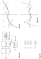
- the Chebyshev nodes x j Ch ⁇ ⁇ 1,1 form a non-equidistant grid, unlike the standard computational basis and Fourier basis associated with equidistant "ruler"-type and "clock”-type grids, as shown in Fig. 2A .
- the Fourier space 206 with an equidistant grid of phases (sectors on a circular open-ended loop with 2 ⁇ j / N arcs) is also shown (bottom).
- Chebyshev feature map for a different kind of feature map. This earlier use refers to a phase-encoded feature map, rather than an amplitude-encoded one.
- the associated "Chebyshev phase space”, as well as the "Chebyshev phase space” associated with the 208 is also shown. Like the Fourier space, this space is defined on the complex plane.
- the ⁇ real' Chebyshev space 204 may also be referred to as the Chebyshev amplitude space.
- Chebyshev feature map in this disclosure refers to the amplitude-encoded Chebyshev feature map.
- Fig. 2B shows the squared overlap between two Chebyshev states
- the Chebyshev overlaps are real, unlike complex overlaps between Fourier states or the earlier phase-encoded Chebyshev-like feature maps, but lead to similar mid-point behaviour.
- the squared overlap can be derived analytically for one of the variables x ' set to one of the Chebyshev nodes, such that ⁇ ⁇ x ′
- ⁇ x ⁇ 2 T N + 1 x ′ T N x ⁇ T N x ′ T N + 1 x 2 N 2 x ′ ⁇ x 2 , which can be derived from the Christofel-Darboux formula for Chebyshev polynomials.
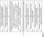
- Fig. 3 is a flow chart describing a method according to an embodiment.
- the method is typically executed by a hybrid quantum computer comprising a classical processor communicatively coupled to a classical memory, and a quantum processor comprising a quantum registry.
- An example of a hybrid quantum computer is described in more detail below with reference to Fig. 17A .
- the classical processor is configured to control the quantum processor.
- the steps as described below are typically performed by the classical processor, but comprise operating the quantum processor.
- a first step 302 comprises determining or receiving a problem description describing a computational problem.
- the computational problem can be, for example, a differential equation problem, a regression problem such as a data regression problem (e.g., combinatorial optimisation), a generative modelling problem, et cetera.
- a step 304 comprises determining or receiving one or more data points related to the computational problem.
- the data points can be, e.g., collocation points, input points associated with output points, et cetera.
- the data points x may have been rescaled to be in the interval x e [-1,1].
- the Chebyshev polynomial can be a Chebyshev polynomial of the first kind or a Chebyshev polynomial of the second kind (commonly denoted as U k ( x )) .
- a step 308 comprises applying the formulated quantum circuit.
- This step typically comprises the classical processor configuring the quantum processor to execute the quantum circuit. Execution of the quantum circuit by the quantum processor transforms the qubits in the quantum register; in this case in accordance with the rules described above.
- a quantum circuit defines a sequence of one or more logical ⁇ quantum gates' for which a hardware implementation is known.
- a hardware implementation typically comprises one or more pulses with a well-defined frequency, amplitude, and duration. Examples of hardware-level schematics of quantum circuits are provided below in, e.g., Figs. 12A-E .
- the formulated quantum circuit may comprise an initialisation part.
- an initialisation circuit may be applied prior to application of the encoding quantum circuit.
- a step 310 comprises receiving or determining one or more additional quantum circuits.
- additional quantum circuits depend on the problem being solved. They may include, e.g., a variational circuit with optimisable parameters. Some examples of additional circuits for various classes of problems are described with reference to Figs. 1A and 9A-B . Depending on the computational problem being solved, some of the one or more additional circuits may be applied prior to application of the encoding quantum circuit.
- a step 312 comprises applying the one or more additional quantum circuits to the quantum register.
- a step 314 comprises receiving measurement data representative of the state of the quantum register.
- the measurement data may be hardware measurement data representing measurements of an output state of the quantum register.
- This step may comprise the classical processor configuring the quantum processor to perform a measurement on at least part of the n qubits in the quantum register.
- a step 316 comprises determining a solution to the computational problem, based on the measurement data and, typically, the problem description.
- the Chebyshev polynomials can be prepared using a combination of exponents for some scaled variable x , where each amplitude is embedded via a phase feature map [ref DQGM].
- the positive and negative phase can be combined using a so-called Linear Combination of Unitaries (LCU) approach, as described in Childs et al., ⁇ Quantum algorithm for systems of linear equations with exponentially improved dependence on precision', SIAM Journal on Computing 46 (2017) pages 1920-1950 .
- LCU Linear Combination of Unitaries
- maps are conditioned on the state of the (top) ancilla qubit, and effectively interfered, choosing the ancilla collapsed to 0 outcome.
- a layer of Hadamard gates is applied to all qubits (including the ancilla) to prepare a superposition of all basis states.
- the first layer corresponds to exp(i x ) and the second layer corresponds to exp(-i 2 x ).
- exp(-i x) exp(i x ) exp(-i 2 x )
- the amplitudes for the basis functions are scaled, based on the variable x such that T k ( x ) are recovered.
- the weight of the constant ( T 0 ( x )) term is adjusted.
- the depicted example uses a round of Grover's iterate circuit 408, rotating the state around
- the measurement operation 412 on the ancilla including the preceding Hadamard gate
- the measurement can be postponed to the end of the circuit. This allows post-selection of the desired state also on systems where only all qubits can be read out simultaneously.
- the layers 402-408 may together be referred to as the Chebyshev feature map 410, as in practice the measurement on the ancilla may often be postponed, with one or more other circuits in between (see, e.g., Fig. 8A and 9A ) .
- the Chebyshev feature map may be represented by a unitary operator U ⁇ ⁇ x .
- Fig. 5A shows the Chebyshev transform which performs the transformation between the Chebyshev and computational bases.
- Fig. 4B schematically shows a quantum circuits for a Fourier feature map (Fourier encoding or spectral encoding), for the sake of comparison.
- This circuit does not use an ancilla.
- Fig. 4C schematically shows a quantum circuits for a phase-encoded Chebyshev-like feature map, for the sake of comparison.
- This circuit does not use an ancilla.
- the feature maps referred to as Chebyshev encoding feature maps in previous disclosures by the present inventors are fundamentally different from the Chebyshev feature map described herein.
- the previously described feature maps have, in general, a non-zero imaginary part, and are not orthonormal. This prevents their conversion to amplitude encoding (which is standard in quantum information processing), and building distributions for generative modelling in particular.
- the currently disclosed Chebyshev feature map is orthonormal and real (i.e., the imaginary part is zero), and may therefore be considered an amplitude encoding.
- FIG. 5A schematically shows an example of a Quantum Chebyshev transform circuit according to an embodiment.
- This circuit maps computational basis states
- j ⁇ j 0 N ⁇ 1 into Chebyshev states
- ⁇ x j Ch ⁇ j 0 N ⁇ 1 .
- this circuit uses an ancillary qubit.
- an Hadamard gate is applied to the ancilla, followed by a CNOT-ladder controlled by the ancilla.
- the transform involves a quantum Fourier transform (QFT) circuit (described below with reference to Fig. 6A ) applied to n + 1 qubits ( n encoding qubits plus one ancilla), followed by phase-adjusting and permutation circuits.
- QFT quantum Fourier transform
- the quantum Chebyshev transform shown in Fig. 5A can be understood as a specific version of the (discrete) cosine transform.
- Fig. 5A shows an alternative approach similar to quantum Fourier transform (QFT) to obtain the quantum Chebyshev transform (QChT) equivalent to DCT II N .
- QFT quantum Fourier transform
- the circuit coverts a complex-valued matrix into a purely real matrix through a series of unitary gates.
- the circuit 500 starts with a Hadamard gate 502 on the ancilla (being considered the most significant bit), followed by a sequence of controlled-NOT gates 504 applied on the other n qubits to create a ( n + 1)-qubit entangled state. This is followed by a ( n + 1) QFT circuit 506 applied to both the ancillary and encoding qubits.
- the resulting state (behind the U 1 gate) has purely real amplitude of
- a permutation circuit 510 is used to reorder amplitudes of the conditioned states, i.e.,
- a permutation circuit identical to block 510 can be appended, in order to obtain the type II discrete sine transform.
- the input and output ancilla bits are initialized with and measured in
- the quantum Chebyshev transform circuit 500 can be run in reverse direction to perform the inverse quantum Chebyshev transform, which equivalently maps Chebyshev basis states
- ⁇ x j Ch ⁇ j 0 N ⁇ 1 to computational basis states
- j ⁇ j 0 N ⁇ 1 . This is shown explicitly in Fig. 5B .
- Fig. 6A schematically shows a Chebyshev feature map circuit according to an embodiment
- Fig. 6B schematically shows a quantum Chebyshev transform circuit according to an embodiment.
- the Chebyshev feature map and quantum Chebyshev transform are applied on the extrema grid, rather than the roots grid, of the Chebyshev polynomials of the first kind of degree k, T k ( x ). This results in different circuits.
- the extrema grid x j Ext ⁇ ⁇ 1,1 forms a non-equidistant grid over [-1,1], which minimizes the problem of Runge's phenomenon associated with a uniform grid.
- a quantum circuit is described that prepares quantum states
- the target state is of the form:
- ⁇ x ⁇ 1 2 ⁇ j 0 + ⁇ jN + 1 ⁇ ⁇ j 0 + ⁇ jN 1 N T 0 x
- 0 ⁇ + 2 N ⁇ k 1 N ⁇ 1 T k x
- ⁇ jk represents the Kronecker-delta function.
- the Chebyshev feature map on the extrema grid shown in Fig. 6A , has essentially the same exp( ⁇ i arccos( x )) phase map configuration 602-606 as that on the roots grid described above with reference to Fig. 4A , layers 402-406; however, in this case, there is one additional qubit.
- the choice of most and least-significant bit (which is in principle an arbitrary choice) has been reversed relative to Fig. 4A .
- constant controlled-rotation gates 610 are applied for adjustment of the weight of the T 0 ( x ) and T N ( x ) terms, corresponding respectively to
- Fig. 6B schematically shows a quantum Chebyshev transform circuit evaluated at the Chebyshev extreme points.
- the quantum Chebyshev transform on the Chebyshev extrema grid maps computational basis states
- j ⁇ j 0 N into Chebyshev states
- ⁇ x j Ext ⁇ j 0 N .
- DCT N I discrete cosine transform matrix
- DCT N I which forms a set of orthonormal basis states:
- the quantum Chebyshev transform on the Chebyshev extrema grid involves a QFT circuit 628 applied to n + 1 qubits (n-qubit system plus one ancilla), similar to the quantum Chebyshev transform on the roots grid shown in Fig. 5A .
- the QFT circuit is sandwiched between constant phase shift/rotation layers 622,634 and permutation layers 626,630.
- the circuit When the input states are of the form
- ⁇ x j Ext ⁇ j 0 N associated with the input
- j ⁇ j 0 N . This corresponds to a matrix with 2N rows, of which the last N - 1 rows contain zero values and can be disregarded.
- M QChTI 2 1 2 cos ⁇ 3 cos ⁇ 4 cos ⁇ 4 cos ⁇ 4 cos ⁇ 3 cos ⁇ 4 cos ⁇ 4 cos 2 ⁇ 4 cos 3 ⁇ 4 ⁇ cos ⁇ 4 cos ⁇ 4 cos 2 ⁇ 4 cos 4 ⁇ 4 cos 6 ⁇ 4 cos ⁇ 4 cos ⁇ 4 cos 3 ⁇ 4 cos 6 ⁇ 4 cos 9 ⁇ 4 ⁇ cos ⁇ 4 cos ⁇ 3 ⁇ cos ⁇ 4 cos ⁇ 4 ⁇ cos ⁇ 4 cos ⁇ 3
- M QChTI (2) Compared with M QChT (2) for the case of Chebyshev nodes, M QChTI (2) reveals one extra row and column in the matrix, which accounts for an additional Chebyshev extreme point.
- the quantum Chebyshev transform circuit can be run in reverse direction to perform the inverse quantum Chebyshev transform, which equivalently maps Chebyshev basis states
- ⁇ x j Ext ⁇ j 0 N back to computational basis states
- j ⁇ j 0 N .
- Fig. 7A schematically shows an example of a quantum Fourier transform circuit, as may be used in layer 506 of the quantum Chebyshev transform shown in Fig. 5A and layer 628 of the quantum Chebyshev transform shown in Fig. 6B .
- Fig. 7B schematically shows an example of an inverse quantum Fourier transform circuit, as may be used in layer 526 of the quantum Chebyshev transform shown in Fig. 5B .
- Chebyshev feature map As mentioned before, one of the advantages of the Chebyshev feature map is that it can be analytically differentiated. This can be utilized in solving differential equations, and learning sensitivities of distributions. The model differentiation can be approached in various ways. These are schematically illustrated in Fig. 8A-C .
- Fig. 8A shows a reference quantum machine learning model (a quantum neural network, QNN-type model).
- the circuit 800 comprises a Chebyshev feature map U ⁇ ⁇ x 802 (corresponding to block 410 in Fig. 4A ), a variational circuit parametrized by a parameter ⁇ and a cost function Re(
- a measurement 808 on the ancilla (corresponding to block 410 ) is included to select the appropriate sum term, as explained above with reference to Fig. 4A .
- One option to differentiate the circuit with respect to the input value x is to use the parameter shift rule, which is well-known in the art, illustrated in Fig. 8C .
- This approach is, for example, valid in the training stage when the cost function corresponds to, for example, a projection on the zero state (including ancilla qubit).
- Application of the parameter shift rule comprises executing the circuit twice for each gate that is dependent on the variable with respect to which the circuit is being differentiated (in this case, the x-dependent gates corresponding to e i x and e -1 2 x , shown in blocks 404 and 406 in Fig.
- an alternative differentiation method may be applied.
- the controlled phase rotations can be decomposed using CNOT conjugation, and two shifts per individually reuploaded parameter x can be applied. This is repeated twice for different bases of the measurement outcomes.
- the Chebyshev feature map can be differentiated with 4 n parameter shifts.
- Fig. 8B Another option, illustrated in Fig. 8B , is to differentiate the feature map formally, extracting an effective generator G ⁇ eff , and taking derivatives as a linear combination of unitaries.
- ⁇ ( x ) ⁇ from eq. (11) is considered, where all the amplitudes are scaled Chebyshev polynomials.
- the normalised version of this is prepared by the Chebyshev feature map.
- the resulting model will contain
- T k ′ x k U k ⁇ 1 x
- U k ( x ) denotes a Chebyshev polynomial of the second kind of order k.
- This means the derivative of a Chebyshev polynomial is a linear combination of lower order Chebyshev polynomials.
- an effective operator G ⁇ eff can be extracted such that:
- ⁇ ′ x ⁇ G ⁇ eff
- the operator G ⁇ eff is non-unitary, but can be implemented using known techniques to implement non-unitary operators, such as a linear combination of unitaries or embedding in a higher-order space.
- ⁇ ⁇ ⁇ 2 N x N ⁇ x ⁇ ⁇ ⁇ x
- N x is the norm of
- Chebyshev feature map and quantum Chebyshev transform can be used to, for example, approximate the distribution of underlying asset prices with the Black-Scholes pricing model.
- Fig. 9A and 9B schematically show, respectively, DQGM training and sampling process according to embodiments.
- Fig. 9A shows a training stage 904 for training quantum neural network
- Fig. 9B shows a sampling stage 910, wherein a quantum circuit is used for generating samples.
- a latent space quantum model representation is used, where a Chebyshev feature map U ⁇ ⁇ x 902 is directly followed by variational circuit U ⁇ ⁇ ⁇ , t 906 and a cost function 918 for measuring the output of the latent space model U ⁇ ⁇ x U ⁇ ⁇ ⁇ , t .
- This latent space quantum model representation may be referred to as a quantum neural network (QNN).
- QNN quantum neural network
- the QNN defines a variational quantum circuit that is trained to represent a function or value, in this particular case a probability density function.
- the training of the QNN includes initialization of the qubits 900 in an initial state, the application of a quantum feature map unitary 902 to map a real parameter x into the Hilbert space (which may be regarded as the "input x to the QNN"), the application of a variational quantum circuit 906 (an Ansatz) parameterized by ⁇ variational parameters' ⁇ , as well as fixed additional parameters t governing the shape of probability distribution that is modelled and a measurement of a cost function value on the qubits of the quantum computer, wherein the cost function value represents the probability density function value evaluated at 918.
- the QNN cost function is assumed to be a ⁇ 0 state or a local cost operator, and can be measured by Hamiltonian averaging, QPE, state-overlap or other operator estimation techniques.
- Fig. 9B shows the sampling stage 910.
- the trained variational circuit 916 is daggered (resulting in an operator U ⁇ ⁇ ⁇ opt , t ⁇ ) and the model from the latent space is mapped to a bit space using quantum Chebyshev transform U ⁇ QChT 912, while the Chebyshev feature map and inverse basis transformation are treated as projective measurement and are subsumed in a sampling process 914.
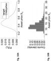
- Fig. 11A and 11B show numerical results of a Chebyshev feature map used for DQGM according to an embodiment.
- an asset is considered whose price follows a geometric Brownian motion under the risk-neutral measure.
- DQGM differentiable quantum generative models
- a mean squared error loss is employed with a learning rate of 0.005, simulated over 5000 epochs using Julia's Yao package.
- the training grid consists of non-negative Chebyshev nodes x j Ch ⁇ j ⁇ 0 , N / 2 , and the evaluation was performed at mid-points between the Chebyshev nodes. It is noted that at the scale used, there is no visible distinction between target and fit.
- the normalized histogram in Fig. 10B shows the resulting sampled distributions, where 10 6 shots are used.
- the success of representing a distribution is defined by the expressivity of the model used to learn it.
- ripples appear in the training distribution where the model is unable to train effectively in-between the training points.
- narrowed lognormal distributions from decreasing volatility are considered, the precision of the training model diminishes as it becomes more difficult to identify the peak of the distribution.
- the figure includes a comparison between training with the quantum Chebyshev model versus training with the quantum Fourier model on the same underlying distribution.
- the derivatives of the respective generative models are shown in Fig. 11B .
- the Chebyshev derivative is more stable than the Fourier derivative (especially close to the boundaries), which is an important consideration for solving differential equations.
- the proposed framework for building quantum models based on Chebyshev models can be used in various ways.
- the preparation of the implicit model can be seen as loading of an amplitude encoded state, which is required for solving systems of linear (and differential) equations.
- Third, the toolkit can be used for solving differential equations, both in the latent space and in the computational space, making the bridge between the two.
- the Chebyshev basis is highly preferred for classical spectral methods, and is de facto a standard in approximation theory.
- mapping allows simple incorporation of boundary conditions with explicit encoding — a problem that has been noted when dealing exclusively with amplitude encoding (i.e., implicit models).
- quantum Chebyshev models can be readily employed in explicit QML models concerning classification, regression, and anomaly detection, both in the variational and kernel-based settings (and targeting cases where high model expressivity is required).
- the Chebyshev feature map and/or quantum Chebyshev transform can also be used outside of a quantum machine learning context.
- the Hamiltonian dynamics exp ⁇ i t H ⁇ can also be seen as an embedding of the time variable t, with features defined by the spectrum of the Hamiltonian .
- an explicit quantum model with spectral features in the Fourier space is obtained. This is usually processed via a QFT for reading out relevant energies.
- alternative quantum walk operators in the modified form of exp exp i arccos t H ⁇ have been shown to lead to significant computational improvements. From the quantum machine learning side, this quantum walk operators implicitly embed Chebyshev-type features. Transforming them into bit-basis states is another use of the quantum Chebyshev transform.
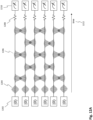
- Fig. 12A is a hardware-level schematic of the actions effectuating the logical operations shown in circuit diagrams such as Figs. 4-9 .
- Unitary operators e.g. those to encode the quantum kernel feature map and derivatives thereof, can be decomposed into a sequence of logical gate operations. These logical gate operations are transformations in a quantum Hilbert space over the qubits encoding an input parameter.
- a classical control stack is used to send pulse information to a pulse controller that affects one or more qubits. The controller may send a sequence of such pulses in time and for each qubit independently.
- An initialization pulse is used to initialize the qubits into the
- a series of single-qubit pulses is sent to the qubit array in 1204, which may apply a single-layer feature map.
- two-qubit pulse sequences can be used to effectively entangle multiple qubits with a feature map 1206.
- the duration, type, strength and shape of these pulses determine the effectuated quantum logical operations.
- 1208 indicates a 'break' in the depicted timeline, which means the sequence of gates may be repeated in a similar fashion in the direction of the time axis 1212. At the end of the pulse sequences, one or more of the qubits are measured 1210.
- Fig. 12B is a hardware-level schematic of the actions effectuating the logical operations shown in circuit diagrams such as Figs. 4-9 , specified for a photonic/optical quantum processor.
- Unitary operators e.g. those used to encode the quantum kernel feature map and derivatives thereof, can be decomposed into a sequence of optical gate operations. These optical gate operations are transformations in the quantum Hilbert space over the optical modes.
- a classical control stack is used to send pulse information to a pulse controller that affects one or more modes.
- the controller may formulate the programmable unitary transformations in a parametrised way.
- the modes 1214 are all in the vacuum state 1216, which are then squeezed to produce single-mode squeezed vacuum states 1218.
- the duration, type, strength and shape of controlled-optical gate transformations determine the effectuated quantum logical operations 1220.
- one or more modes are measured with photon-number resolving, Fock basis measurement 1222, tomography or threshold detectors.
- Fig. 12C is a hardware-level schematic of the actions effectuating the logical operations shown in circuit diagrams such as Figs. 4-9 , specified for a Gaussian boson sampling device.
- Unitary operators e.g. those used to encode the quantum kernel feature map and derivatives thereof, can be decomposed into a sequence of optical gate operations. These optical gate operations are transformations in the quantum Hilbert space over the optical modes.
- a classical control stack is used to send information to optical switches and delay lines.
- the controller may formulate the programmable unitary transformations in a parametrised way.
- the modes 1226 are all in a weak coherent state, which is mostly a vacuum state with a chance of one or two photons and negligibly so for higher counts. Subsequently, the photons travel through optical waveguides 1228 through delay lines 1230 and two-mode couplers 1232 which can be tuned with a classical control stack, and which determines the effectuated quantum logical operations.
- one or more modes are measured with photon-number resolving 1234, or threshold detectors.
- Fig. 12D is a hardware-level schematic of the actions effectuating the logical operations shown in circuit diagrams such as Figs. 4-9 , which may be executed on a neutral-atom-based quantum computer.
- unitary operators e.g. those used to encode the quantum feature map and derivatives thereof, can be decomposed in two different kinds of operations: digital or analog. Both of these operations are transformations in the quantum Hilbert space over atomic states.
- FIG. 12D Schematic (a) of Fig. 12D depicts a digital quantum circuit 1238, wherein local laser pulses may be used to individually address neutral atoms to effectuate transitions between atomic states which effectively implement sets of standardized or 'digital' rotations on computational states.
- These digital gates may include any single-qubit rotations, and a controlled-pauli-Z operation with arbitrary number of control qubits. Additionally, such digital gate operations may also include 2-qubit operations.
- FIG. 12D Schematic (b) of Fig. 12D depicts an analog mode 1246 of operation, wherein a global laser light pulse may be applied to groups of, or all, atoms at the same time, with certain properties like detuning, Rabi frequencies and Rydberg interactions to cause multi-qubit entanglement thereby effectively driving the evolution of a Hamiltonian 1244 of the atomic array in an analog way.
- FIG. 12D depicts an example of such digital-analog quantum circuit, including blocks 1246 1-3 of digital qubit operations (single or multi-qubit) and analog blocks 1248 1-3 .
- Digital-analog circuits define circuits which are decomposed into both explicitly-digital and explicitly-analog operations. While under the hood, both are implemented as evolutions over controlled system Hamiltonians, the digital ones form a small set of pre-compiled operations, typically but not exclusively on single-qubits, while analog ones are used to evolve the system over its natural Hamiltonian, for example in order to achieve complex entangling dynamics.
- digital-analog quantum circuits for a neutral quantum processor that are based on Rydberg type of Hamiltonians can be differentiated analytically so that they can be used in variational and/or quantum machine learning schemes, including the differential quantum circuit (DQC) schemes as described in this application.
- DQC differential quantum circuit
- a classical control stack is used to send information to optical components and lasers.
- the controller may formulate the programmable unitary transformations in a parametrised way.
- the states of one or more atoms may be read out by applying measurement laser pulses, and then observing the brightness using a camera to spot which atomic qubit is turned 'on' or 'off', 1 or 0. This bit information across the array is then processed further according to the embodiments.
- Fig. 12E is a hardware-level schematic of the actions effectuating the logical operations shown in Figs. 4-9 , specified for a photonic/optical quantum processor.
- the quantum model can be decomposed into a sequence of optical gate operations. These optical gate operations are transformations in the quantum Hilbert space of the photons.
- a classical control stack is used to send information to a universal multiport interferometer.
- the controller may formulate the programmable unitary transformations in a parameterized way.
- the photons 1255 are in Fock states, weak coherent states or coherent states.
- the duration, type, strength and shape of controlled-optical gate transformations determine the effectuated quantum logical operations 1256.
- the modes are measured with photon-number resolving, Fock basis measurement 1257, tomography or threshold detectors.
- Fig. 12A-12E may also be used to implement the quantum circuits shown in Fig. 13-16 , as applicable.
- Fig. 13A depicts a system describing a Digital-Analog implementation of a quantum algorithm.
- Fig. 13A represents a Digital-Analog implementation where the qubit interactions can be switched on and off and there exists single-qubit addressability for the application of single-qubit gates, a process described in 1300.
- a classical control stack may be used to send information to a controller that affects one or more qubits.
- the controller may send multiple information carriers (e.g., pulses) in time and for each qubit independently.
- An initialization protocol is used to initialize the qubits, in this example into the
- the current example shows only four qubits, but the same principles may be extended in a straightforward manner to systems with more (or less) than four qubits.
- a quantum feature map is applied 1304 to encode quantum information, e.g., an input variable, into a Hilbert space associated with the quantum processor.
- the variational Ansatz comprises three single-qubit gates R Y - R X - R Y with different rotational angles ⁇ i .
- These single-qubit gates are typically sets of standardized or 'digital' rotations on computational states applied to different qubits with different rotation angles/parameters.
- These digital gates include any single-qubit rotations according to the ⁇ i argument of the rotation.
- a single rotation/single-qubit gate is not sufficient to perform arbitrary rotation regardless of the parameter/angle since it can only rotate over a single axis.
- three gates in series with different rotation angles/parameters can be used, in this example represented by a block of single-qubit gates 1306.
- a parametric analog unitary block can be applied, which entangles the atoms and can act as a variational Ansatz.
- the wavefunction may be evolved once more, and finally a measurement in the computational basis occurs as described in 1310.
- additional steps may be included, represented by the ellipses, e.g., before, after, or in between the blocks shown.
- a different initial state than 10 may be prepared prior to application of the feature map.
- the blocks can be executed in a different order, for instance, in some embodiments, block 1308 might precede block 1306.
- One or more of the blocks 1304-1308, or variations thereof, may be repeated one or more times prior to the measurement 1310.
- Fig. 13B represents a typical quantum feature map 1312 that starts by preparing the quantum register to the 10) quantum state 1302 and then applying single-qubit rotations in all of the qubits with (typically) different rotation angles 1304.
- single qubit rotations 1304 (here chosen as R Y ( f i ( x )) act on each qubit individually and are parametrized by a variable x .
- the variable x may be used as an angle of rotation.
- the application 1304 of one rotation operation to each qubit in a register may be referred to as a single layer of rotation operations.
- This type of encoding of classical information into quantum states is known as angle encoding, which means that a data vector is represented by the angles of a quantum state.
- Fig. 13C illustrates different pulses (potentially differing in pulse duration and/or amplitude/height) that can be sent to the quantum circuit (different qubits) to encode the classical information.
- the angle of the rotation that is described by the f i ( x ) dictates the duration and geometry of the pulse.
- Fig. 14A presents a quantum circuit based on a Digital-Analog implementation 1400 that has no single-qubit addressability and uses a wavefunction evolution that can be turned on and off for the entanglement generation.
- Fig. 14A differs from Fig. 13A in that it shows a technique known as data re-uploading that alters the quantum feature map 1404 and 1410. Loading classical data into a quantum system is a non-trivial task, and uploading large amounts of data makes it an even more critical issue. However, when the case of big-data is not considered, techniques like data re-uploading can be utilized.
- Such a data re-uploading technique may start by setting the quantum register to an initial state, e.g., the all-zero state 1402, followed by angle encoding that is based on a feature map 1404, in this case a tower feature map.
- the classical data are re-uploaded through angle encoding into single-qubit rotations 1410.
- the information is encoded using different angles than in the previous data uploading steps.
- the amount of rotation may be doubled in each data (re-)uploading step 1404,1410 (i.e., the rotational angle of the might be increasing as 1-2-4, etc.).
- the rotations R Y - R X - R Y are applied to all qubits simultaneously with the same rotation angle for each single qubit gate, but different than 1406.
- the classical information can be repeatedly encoded into the quantum feature map through the data re-uploading technique, while changing the angle of the single qubit rotational angle ( 1404, 1410, etc.) every time after the wavefunction evolution.
- the resulting quantum feature map can become more expressive as a tower feature map by doing this process of serial data re-uploading with different levels of rotational angles every time the re-uploading is done.
- Fig. 14B illustrates a different (and at current technology levels more realistic) form of a Digital-Analog implementation.
- the system has single-qubit addressability, but the wavefunction evolution cannot be turned off, thus staying always on.
- This system requires less control over the qubit interactions (since they are always on) and only requires single-qubit addressability.
- the single-qubit gates are applied while the wavefunction evolution (qubit interaction) is also happening.
- the quantum circuit 1418 starts by encoding information in the 10) quantum state 1402, followed by a quantum feature map 1404 (analogous to 1304 ).
- a variational Ansatz comprising both wavefunction evolution e ⁇ i H t 1408 and simultaneous application of a block of single-qubit gates 1416 (similar to block 1306 ). After multiple repetitions of block 1416, each time with different rotational angles at the single-qubit gates, the circuit ends with a measurement in the computational basis 1414.
- Fig. 15A illustrates a quantum circuit 1500 that implements a Digital-Analog implementation with single-qubit addressability, wherein the wavefunction evolution (e.g., atom interactions) can be turned on and off.
- the same technique of data re-uploading with a tower feature map 1504, 1510 and the same Ansatz comprising single-qubit gates 1506,1512 followed by wavefunction evolution 1508 are used (all similar to 1400 ).
- Fig. 15B illustrates a quantum circuit that implements a Digital-Analog implementation with single-qubit addressability 1518, similar to 1500, but with the entanglement generated via CZ gates between the qubits, resembling the atom interaction / entanglement generation.
- Fig. 16 presents a workflow for generalized circuit differentiation.
- QML Quantum Machine Learning
- PQCs Parametric Quantum Circuits
- These quantum circuits contain tuneable parameters that use a classical optimizer to find the optimal values of the parameters that exist for that formulation.
- the differentiation required for most parameter optimization methods can be achieved in various ways, with the most common one being the Parameter Shift Rule (PSR).
- PSR Parameter Shift Rule
- GPSR Generalized Parametric Shift Rule
- Fig. 17A depicts a system for determining a solution for an computational problem using a hybrid quantum computer system according to an embodiment.
- the system 1702 may include a quantum computer system 1704 comprising one or more quantum processors 1708, e.g. a gate-based qubit quantum processor, and a controller system 1710 comprising input output (I/O) devices which form an interface between the quantum processor and the outside world, e.g., the one or more classical processors of a classical computer 1706.
- the controller system may include a system for generating control signals for controlling the quantum processing elements.
- the control signals may include for example a sequence of pulses, e.g. microwave pulses, voltage pulses and/or optical pulses, which are used to manipulate qubits.
- the controller may include output device, e.g. readout circuits, for readout of the qubits and the control signals for readout of the quantum processing elements, e.g. a readout pulse for reading a qubit.
- output device e.g. readout circuits
- the control signals for readout of the quantum processing elements e.g. a readout pulse for reading a qubit.
- at least a part such readout circuit may be located or integrated with the chip that includes the qubits.
- the system may further comprise a (purely classical information) input 1712 and an (purely classical information) output 1714.
- the data processor systems may be configured to solve an optimization problem using the quantum computer.
- Input data may include information about the optimisation problem one wishes to solve. This information may include training data such as input-output pairs, a differential equation, boundary conditions, initial values, regularization values, etc.
- the input data may be used by the system to construct quantum circuits, in particular quantum feature maps and/or parametrized quantum circuits, and to classically calculate values, e.g. sequences of pulses, which may be used to initialize and control qubit operations according to the quantum circuit.
- the classical computer may include a quantum circuit generator 1707.
- the input data may be used by the system to classically calculate values, e.g. parameter settings, which may be used to initialize the quantum circuit that is implemented on the quantum processor.
- output data may include loss function values, sampling results, correlator operator expectation values, optimisation convergence results, optimized quantum circuit parameters and hyperparameters
- Each of the one or more quantum processors may comprise a set of controllable quantum processing elements, e.g. a set of controllable two-level systems referred to as qubits.
- the two levels are
- the embodiments in this application are not limited to qubits but may include any multi-level quantum processing elements, e.g. qutrits, that is suitable for performing quantum computation.
- Examples of such quantum processors include noisy intermediate-scale quantum (NISQ) computing devices and fault tolerant quantum computing (FTQC) devices.
- NISQ noisy intermediate-scale quantum
- FTQC fault tolerant quantum computing
- the quantum processor may be configured to execute a quantum algorithm in accordance with the gate operations of a quantum circuit.
- the quantum processor may be implemented as a gate-based qubit quantum device, which allows initialization of the qubits into an initial state, interactions between the qubits by sequentially applying quantum gates between different qubits and subsequent measurement of the qubits' states.
- the input devices may be configured to configure the quantum processor in an initial state and to control gates that realize interactions between the qubits.
- the output devices may include readout circuitry for readout of the qubits which may be used to determine a measure of the energy associated with the expectation value of the Hamiltonian of the system taken over the prepared state.
- the one or more quantum processors may comprise a set of continuous variable systems, such as optical or photonic quantum computers.
- the quantum processor may comprise a Gaussian Boson Sampling device as described above with reference to Fig. 12C or any of the other hardware described above with reference to Fig. 12A-E .
- the first data processor system may be implemented as a software program for simulating a quantum computer system 1704 comprising a quantum processor system 1708.
- the software program may be a classical software program that runs a classical computer 1706 so that quantum algorithms can be developed, executed and tested on a classical computer without requiring access to a hardware implementation of the quantum processor system.
- Fig. 17B is a block diagram illustrating an exemplary classical data processing system described in this disclosure, for example classical computer 1706.
- Classical data processing system 1720 may include at least one processor 1722 coupled to memory elements 1724 through a system bus 1726. As such, the data processing system may store program code within memory elements 1724. Further, processor 1722 may execute the program code accessed from memory elements 1724 via system bus 1726.
- data processing system may be implemented as a computer that is suitable for storing and/or executing program code. It should be appreciated, however, that data processing system 1720 may be implemented in the form of any system including a processor and memory that is capable of performing the functions described within this specification.
- Memory elements 1724 may include one or more physical memory devices such as, for example, local memory 1728 and one or more bulk storage devices 1730.
- Local memory may refer to random access memory or other non-persistent memory device(s) generally used during actual execution of the program code.
- a bulk storage device may be implemented as a hard drive or other persistent data storage device.
- the classical data processing system 1720 may also include one or more cache memories (not shown) that provide temporary storage of at least some program code in order to reduce the number of times program code must be retrieved from bulk storage device 1730 during execution.
- I/O devices depicted as key device 1732 and output device 1734 optionally can be coupled to the data processing system.
- key device may include, but are not limited to, for example, a keyboard, a pointing device such as a mouse, or the like.
- output device may include, but are not limited to, for example, a monitor or display, speakers, or the like.
- Key device and/or output device may be coupled to data processing system either directly or through intervening I/O controllers.
- a network adapter 1736 may also be coupled to data processing system to enable it to become coupled to other systems, computer systems, remote network devices, and/or remote storage devices through intervening private or public networks.
- the network adapter may comprise a data receiver for receiving data that is transmitted by said systems, devices and/or networks to said data and a data transmitter for transmitting data to said systems, devices and/or networks.
- Operation modems, cable operation modems, and Ethernet cards are examples of different types of network adapter that may be used with classical data processing system 1720.
- memory elements 1724 may store an application 1738.
- classical data processing system 1720 may further execute an operating system (not shown) that can facilitate execution of the application.
- Application being implemented in the form of executable program code, can be executed by classical data processing system 1720, e.g., by processor 1722. Responsive to executing application, data processing system may be configured to perform one or more operations to be described herein in further detail.
- classical data processing system 1720 may represent a client data processing system.
- application 1738 may represent a client application that, when executed, configures classical data processing system 1720 to perform the various functions described herein with reference to a "client".
- client can include, but are not limited to, a personal computer, a portable computer, a mobile phone, or the like.
- data processing system may represent a server.
- data processing system may represent an (HTTP) server in which case application 1738, when executed, may configure data processing system to perform (HTTP) server operations.
- data processing system may represent a module, unit or function as referred to in this specification.
Landscapes
- Engineering & Computer Science (AREA)
- General Physics & Mathematics (AREA)
- Theoretical Computer Science (AREA)
- Physics & Mathematics (AREA)
- Mathematical Analysis (AREA)
- Computing Systems (AREA)
- Evolutionary Computation (AREA)
- Condensed Matter Physics & Semiconductors (AREA)
- Computational Mathematics (AREA)
- Mathematical Optimization (AREA)
- Pure & Applied Mathematics (AREA)
- Data Mining & Analysis (AREA)
- General Engineering & Computer Science (AREA)
- Mathematical Physics (AREA)
- Software Systems (AREA)
- Artificial Intelligence (AREA)
- Complex Calculations (AREA)
- Optical Modulation, Optical Deflection, Nonlinear Optics, Optical Demodulation, Optical Logic Elements (AREA)
Priority Applications (2)
| Application Number | Priority Date | Filing Date | Title |
|---|---|---|---|
| EP23182499.6A EP4485293A1 (de) | 2023-06-29 | 2023-06-29 | Quantum-chebyschv-kodierung |
| PCT/EP2024/062353 WO2025002636A1 (en) | 2023-06-29 | 2024-05-03 | Real quantum feature map encoding |
Applications Claiming Priority (1)
| Application Number | Priority Date | Filing Date | Title |
|---|---|---|---|
| EP23182499.6A EP4485293A1 (de) | 2023-06-29 | 2023-06-29 | Quantum-chebyschv-kodierung |
Publications (1)
| Publication Number | Publication Date |
|---|---|
| EP4485293A1 true EP4485293A1 (de) | 2025-01-01 |
Family
ID=87060625
Family Applications (1)
| Application Number | Title | Priority Date | Filing Date |
|---|---|---|---|
| EP23182499.6A Withdrawn EP4485293A1 (de) | 2023-06-29 | 2023-06-29 | Quantum-chebyschv-kodierung |
Country Status (2)
| Country | Link |
|---|---|
| EP (1) | EP4485293A1 (de) |
| WO (1) | WO2025002636A1 (de) |
Families Citing this family (3)
| Publication number | Priority date | Publication date | Assignee | Title |
|---|---|---|---|---|
| US12450952B1 (en) | 2024-11-26 | 2025-10-21 | Daon Technology | Methods and systems for enhancing detection of morphed biometric modality data |
| US12413402B1 (en) * | 2025-01-23 | 2025-09-09 | Daon Technology | Methods and systems for enhancing detection of fraudulent authentication data |
| CN119783842B (zh) * | 2025-03-13 | 2025-07-15 | 国开启科量子技术(安徽)有限公司 | 量子态振幅编码方法、装置、设备及介质 |
Citations (1)
| Publication number | Priority date | Publication date | Assignee | Title |
|---|---|---|---|---|
| WO2022101483A1 (en) | 2020-11-15 | 2022-05-19 | Qu & Co R&D B.V. | Solving a set of (non)linear differential equations using a hybrid data processing system comprising a classical computer system and a quantum computer system |
Family Cites Families (1)
| Publication number | Priority date | Publication date | Assignee | Title |
|---|---|---|---|---|
| EP4224378A1 (de) | 2022-02-07 | 2023-08-09 | Qu&CO R&D B.V. | Differenzierbare generative modellierung unter verwendung eines hybriden computers mit einem quantenprozessor |
-
2023
- 2023-06-29 EP EP23182499.6A patent/EP4485293A1/de not_active Withdrawn
-
2024
- 2024-05-03 WO PCT/EP2024/062353 patent/WO2025002636A1/en not_active Ceased
Patent Citations (1)
| Publication number | Priority date | Publication date | Assignee | Title |
|---|---|---|---|---|
| WO2022101483A1 (en) | 2020-11-15 | 2022-05-19 | Qu & Co R&D B.V. | Solving a set of (non)linear differential equations using a hybrid data processing system comprising a classical computer system and a quantum computer system |
Non-Patent Citations (8)
| Title |
|---|
| ANNIE E PAINE ET AL: "Quantum Quantile Mechanics: Solving Stochastic Differential Equations for Generating Time-Series", ARXIV.ORG, CORNELL UNIVERSITY LIBRARY, 201 OLIN LIBRARY CORNELL UNIVERSITY ITHACA, NY 14853, 3 October 2021 (2021-10-03), XP091069400 * |
| CHELSEA A WILLIAMS ET AL: "Quantum Chebyshev Transform: Mapping, Embedding, Learning and Sampling Distributions", ARXIV.ORG, CORNELL UNIVERSITY LIBRARY, 201 OLIN LIBRARY CORNELL UNIVERSITY ITHACA, NY 14853, 29 June 2023 (2023-06-29), XP091550452 * |
| CHILDS ET AL.: "Quantum algorithm for systems of linear equations with exponentially improved dependence on precision", SIAM JOURNAL ON COMPUTING, vol. 46, 2017, pages 1920 - 1950 |
| KLAPPENECKER ET AL.: "Discrete Cosine Transforms on Quantum Computers", IEEE R8-EURASIP SYMPOSIUM ON IMAGE AND SIGNAL PROCESSING AND ANALYSIS (PULA, CROATIA, 2001, pages 464 - 468 |
| KYRIIENKO ET AL.: "Generalized quantum circuit differentiation rules", PHYS. REV. A, vol. 104, no. 052417 |
| KYRIIENKO OLEKSANDR ET AL: "Protocols for Trainable and Differentiable Quantum Generative Modelling", 16 February 2022 (2022-02-16), XP055980124, Retrieved from the Internet <URL:https://arxiv.org/pdf/2202.08253.pdf> [retrieved on 20221110] * |
| M. SCHULD ET AL.: "Quantum machine learning in feature Hilbert spaces", PHYS. REV. LETT., vol. 122, 2019, pages 040504 |
| OLEKSANDR KYRIIENKO ET AL: "Solving nonlinear differential equations with differentiable quantum circuits", ARXIV.ORG, CORNELL UNIVERSITY LIBRARY, 201 OLIN LIBRARY CORNELL UNIVERSITY ITHACA, NY 14853, 18 May 2021 (2021-05-18), XP081951791, DOI: 10.1103/PHYSREVA.103.052416 * |
Also Published As
| Publication number | Publication date |
|---|---|
| WO2025002636A1 (en) | 2025-01-02 |
Similar Documents
| Publication | Publication Date | Title |
|---|---|---|
| EP4485293A1 (de) | Quantum-chebyschv-kodierung | |
| Metz et al. | Self-correcting quantum many-body control using reinforcement learning with tensor networks | |
| Huang et al. | Predicting many properties of a quantum system from very few measurements | |
| US12340277B2 (en) | Hybrid quantum-classical computer for solving linear systems | |
| US11966707B2 (en) | Quantum enhanced word embedding for natural language processing | |
| EP4104114B1 (de) | Hybrider quantenklassischer adversarischer generator | |
| US20220292385A1 (en) | Flexible initializer for arbitrarily-sized parametrized quantum circuits | |
| US20250299084A1 (en) | Quantum extremal learning | |
| US10417574B2 (en) | Embedding electronic structure in controllable quantum systems | |
| Lazzarin et al. | Multi-class quantum classifiers with tensor network circuits for quantum phase recognition | |
| Saleem et al. | Approaches to constrained quantum approximate optimization | |
| EP4381424A1 (de) | Verfahren und systeme zur lösung einer stochastischen differentialgleichung unter verwendung eines hybriden computersystems | |
| EP4495841A1 (de) | Lösung von rechenproblemen unter verwendung von trainierbaren quantenmerkmalskarten | |
| US20250139487A1 (en) | Differentiable generative modelling using a hybrid computer including a quantum processor | |
| US20250181950A1 (en) | Quantum-kernel-based regression | |
| Umeano et al. | What can we learn from quantum convolutional neural networks? | |
| EP4339847A1 (de) | Effizientes training eines quantenabtasters | |
| He et al. | Quantum Gaussian filter for exploring ground-state properties | |
| Williams et al. | Quantum Chebyshev transform: mapping, embedding, learning and sampling distributions | |
| Schuld et al. | Representing data on a quantum computer | |
| Atchade-Adelomou et al. | Fourier series weight in quantum machine learning | |
| EP4273760A1 (de) | Quantenextremlernen | |
| EP4495844A1 (de) | Quantenschaltungen | |
| EP4575919A1 (de) | Abgeleitete quantenschaltungen | |
| EP4530938A1 (de) | Schusseffizienter quantensolver für differentialgleichungen |
Legal Events
| Date | Code | Title | Description |
|---|---|---|---|
| PUAI | Public reference made under article 153(3) epc to a published international application that has entered the european phase |
Free format text: ORIGINAL CODE: 0009012 |
|
| STAA | Information on the status of an ep patent application or granted ep patent |
Free format text: STATUS: THE APPLICATION HAS BEEN PUBLISHED |
|
| AK | Designated contracting states |
Kind code of ref document: A1 Designated state(s): AL AT BE BG CH CY CZ DE DK EE ES FI FR GB GR HR HU IE IS IT LI LT LU LV MC ME MK MT NL NO PL PT RO RS SE SI SK SM TR |
|
| STAA | Information on the status of an ep patent application or granted ep patent |
Free format text: STATUS: THE APPLICATION IS DEEMED TO BE WITHDRAWN |
|
| 18D | Application deemed to be withdrawn |
Effective date: 20250702 |
|
| 19U | Interruption of proceedings before grant |
Effective date: 20250624 |
|
| 19W | Proceedings resumed before grant after interruption of proceedings |
Effective date: 20260202 |
|
| STAA | Information on the status of an ep patent application or granted ep patent |
Free format text: STATUS: THE APPLICATION HAS BEEN PUBLISHED |