EP4459495A2 - Erkennung von bereichen mit hoher krümmung auf kurven - Google Patents
Erkennung von bereichen mit hoher krümmung auf kurven Download PDFInfo
- Publication number
- EP4459495A2 EP4459495A2 EP24174221.2A EP24174221A EP4459495A2 EP 4459495 A2 EP4459495 A2 EP 4459495A2 EP 24174221 A EP24174221 A EP 24174221A EP 4459495 A2 EP4459495 A2 EP 4459495A2
- Authority
- EP
- European Patent Office
- Prior art keywords
- automatically
- curve function
- curve
- arc length
- function
- Prior art date
- Legal status (The legal status is an assumption and is not a legal conclusion. Google has not performed a legal analysis and makes no representation as to the accuracy of the status listed.)
- Pending
Links
Images



Classifications
-
- G—PHYSICS
- G06—COMPUTING OR CALCULATING; COUNTING
- G06T—IMAGE DATA PROCESSING OR GENERATION, IN GENERAL
- G06T17/00—Three-dimensional [3D] modelling for computer graphics
- G06T17/30—Polynomial surface description
-
- G—PHYSICS
- G06—COMPUTING OR CALCULATING; COUNTING
- G06F—ELECTRIC DIGITAL DATA PROCESSING
- G06F9/00—Arrangements for program control, e.g. control units
- G06F9/06—Arrangements for program control, e.g. control units using stored programs, i.e. using an internal store of processing equipment to receive or retain programs
- G06F9/30—Arrangements for executing machine instructions, e.g. instruction decode
- G06F9/30003—Arrangements for executing specific machine instructions
- G06F9/30007—Arrangements for executing specific machine instructions to perform operations on data operands
- G06F9/3001—Arithmetic instructions
-
- G—PHYSICS
- G06—COMPUTING OR CALCULATING; COUNTING
- G06F—ELECTRIC DIGITAL DATA PROCESSING
- G06F30/00—Computer-aided design [CAD]
- G06F30/10—Geometric CAD
- G06F30/15—Vehicle, aircraft or watercraft design
-
- G—PHYSICS
- G06—COMPUTING OR CALCULATING; COUNTING
- G06F—ELECTRIC DIGITAL DATA PROCESSING
- G06F17/00—Digital computing or data processing equipment or methods, specially adapted for specific functions
- G06F17/10—Complex mathematical operations
- G06F17/11—Complex mathematical operations for solving equations, e.g. nonlinear equations, general mathematical optimization problems
-
- G—PHYSICS
- G06—COMPUTING OR CALCULATING; COUNTING
- G06F—ELECTRIC DIGITAL DATA PROCESSING
- G06F17/00—Digital computing or data processing equipment or methods, specially adapted for specific functions
- G06F17/10—Complex mathematical operations
- G06F17/15—Correlation function computation including computation of convolution operations
- G06F17/153—Multidimensional correlation or convolution
-
- G—PHYSICS
- G06—COMPUTING OR CALCULATING; COUNTING
- G06F—ELECTRIC DIGITAL DATA PROCESSING
- G06F30/00—Computer-aided design [CAD]
- G06F30/10—Geometric CAD
- G06F30/17—Mechanical parametric or variational design
-
- G—PHYSICS
- G06—COMPUTING OR CALCULATING; COUNTING
- G06F—ELECTRIC DIGITAL DATA PROCESSING
- G06F30/00—Computer-aided design [CAD]
- G06F30/20—Design optimisation, verification or simulation
-
- G—PHYSICS
- G06—COMPUTING OR CALCULATING; COUNTING
- G06F—ELECTRIC DIGITAL DATA PROCESSING
- G06F2113/00—Details relating to the application field
- G06F2113/28—Fuselage, exterior or interior
Definitions
- the field of the present disclosure relates generally to systems and methods of analyzing two-dimensional curves and three-dimensional (3D) models of object surfaces, and more specifically, to detecting features of such geometries.
- CAD computer-aided design
- CAM computer-aided manufacturing
- CAE computer-aided engineering
- the process of reconstructing a multi-sheet model into a single-cell surface is computationally expensive. If a CAD model is only stored as a multi-piece design, recurring costs may be incurred to take the multi-piece model and refit a single surface so for each analysis that is to be performed.
- any curves of the model may be desirable to determine the quality of any curves of the model, to identify the boundaries of the part, the sides and/or corners of the part, and/or other curvature-based features, such as areas of sudden or rapid curvature.
- a method for detecting regions of high curvature on a curve.
- the method comprises receiving a curve function and automatically arc length parameterizing the curve function.
- the local average curvature over the arc length parameterized curve function is automatically computed.
- One or more regions where the local average curvature turns at least a predetermined angle over a given interval are automatically indicated.
- the indicated regions are then output.
- Complex objects and surfaces may be stored as a plurality of segments that can individually be described with reasonably simple mathematical descriptors. Increasing the size and complexity of the segment may increase such complexity, thereby occupying more storage space for the same object.
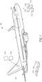
- FIG. 1 depicts a three-dimensional model in the form of an aircraft model 100, according to some examples.
- a three-dimensional computer model for aircraft model 100 can be segmented into a number of different portions, referred to herein as sheets.
- the sheets are discrete in the sense that they are non-coextensive relative to specific discrete components of the three-dimensional model.
- the sheets may be relatively small square or rectangular pieces that are not recognizable as any distinct portion of the three-dimensional model.
- a fairing of aircraft model 100 may be broken up into hundreds of sheets or more, none of which would be recognizable as a fairing.
- Aircraft model 100 has a rudder region 102 which is part of the aircraft rudder, a wing region 104 which is part of the right wing of the aircraft, and a canopy region 106 which is part of the canopy covering the cockpit.
- the regions are decomposed into sheets 110.
- two exemplary sheets 110a and 110b are shown for rudder region 102; three exemplary sheets 110c, 110d, and 110e are shown for wing region 104; and four exemplary sheets 110f, 110g, 110h, and 110i are shown for canopy region 106.
- a boundary can be defined as a plurality of curves, or as a spline comprising a plurality of knots. For each knot, the derivative immediately before and after the knot can be compared for any sudden changes.
- this approach will miss features that can occur in between knots or that only present themselves across several knots.
- the model can be flattened from 3D to 2D, then the resulting surface discretized at a large number of points.
- human guidance is required to select the flattening algorithm, and thus this process is not conducive to automation. Further, some models are not feasible to flatten.
- a curve for a model is arc length parameterized.
- Spline Math can be used to compute curvature.
- the curvature can then be convolved to generate curvature averages along the boundary curves.
- the dot product of this averaged curvature with itself yields a univariate function that can be employed to detect and identify the location of features on the curve.
- Such features may include intervals where the curve is turning sharply, and corners or other such detecting points of maximal locally-averaged curvature. While generally described in the context of curves derived from single cell surfaces of 3D models, the systems and methods described herein may be applied broadly to the analysis of curves from any source.
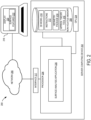
- FIG. 2 a schematic diagram of a surface analysis system 200 is depicted, comprising a server computing device 202 which includes one or more processors 204, which can be communicatively coupled to a network 206.
- the server computing device 202 further comprises non-volatile memory 208 storing a three-dimensional (3D) virtual model 210 and instructions 212 that, when executed by the processor 204, cause the processor 204 to retrieve the 3D virtual model 210 from the non-volatile memory 208.
- the 3D virtual model 210 can be of an aircraft or an aircraft component, or other manufactured parts or components, for example, as illustrated in FIG. 1 .
- the sizes of the 3D virtual model 210 are not particularly limited-the 3D virtual model 210 can be of micron-scale objects in such applications as printed circuit boards or medical devices, or of over-sized objects.
- the 3D virtual model 210 is a mathematical representation of the surface geometry of an object, so that computer-rendered images of the object can be created from any angle.
- the 3D virtual model 210 can be a polygon mesh model that includes one or more object surfaces.
- 3D virtual model 210 includes a plurality of sub-models and object portions, of which two or more adjacent sub-models or object portions may be combined into a single, continuous model with contiguous object surfaces.
- Geometry package 214 that can approximate or represent geometrical surfaces as functions. For example, for each parameterized curve of 3D virtual model 210, an input value in parameter space (t) may be provided, and geometry package 214 may return a position in (x,y,z) space where (t) lies on the curve (e.g., a spline). In some examples, geometry package 214 may be employed so that one or more feature curves of the 3D virtual model 210 can be projected to produce a plurality of two-dimensional curves (U-V curves).
- the U-V mapping is a parameterized surface and can be a piecewise polynomial mapping, such as a tensor product spline, between a two-dimensional rectangular parameter domain and three-dimensional space.
- Approximation theory tool 216 may represent curves of 3D virtual model as parametric curves.
- Approximation theory tool 216 may include CAD packages and/or other tools with similar functions. Additional mathematical libraries and packages may be included in approximation theory tool 216, and employed to extract the boundary pieces from faces of object surfaces, represent those boundary pieces as parametric curves, and to join the set of parametric curves as a single parametric curve.
- the server computing device 202 includes a network interface 217 to affect the communicative coupling to the network 206 and, through the network 206, a client computing device 218.
- the client computing device 218 comprises a display 220 which is configured to display surface features 222 and other graphical analysis of object surfaces which are output by the server computing device 202.
- Network interface 217 can include a physical network interface, such as a network adapter.
- the server computing device 202 can be a special-purpose computer, adapted for reliability and high-bandwidth communications.
- the system 200 can be embodied in a cluster of individual hardware server computers, for example.
- the processor 204 can be multi-core processors suitable for handling large amounts of information.
- the processor 204 is communicatively coupled to non-volatile memory 208 storing a 3D virtual model 210 including one or more object surfaces, geometry package 214, approximation theory tool 216, and instructions 212 which can be executed by the processor 204 to effectuate the techniques disclosed herein on concert with the client computing device 218 as shown and described below.
- the non-volatile memory 208 can be in a Redundant Array of Inexpensive Disk drives (RAID) configuration for added reliability.
- the processor 204 can also be communicatively coupled to graphical co-processors (GPU) 224. Graphical co-processors 224 can expedite the technique disclosed herein by performing operations in parallel.
- GPU
- the processor 204 is configured to execute a surface analysis application 226.
- the surface analysis application 226 is configured to receive a curve function defining a portion of an object surface retrieved from a 3D virtual model 210 of an object from the non-volatile memory 208, arc length parameterize the curve function, compute local average curvature over the arc length parameterized curve function, indicate one or more regions where the local average curvature turns at least a predetermined angle over a given interval in parameter space.
- the surface analysis application 226 is further configured to parameterize the curve function to a single variable, convolving a derivative of the curve function to obtain a first convolution, convolve the first convolution to obtain a second convolution, and to indicate a predetermined number of points of the second convolution having maximal values.
- Surface analysis application 226 is further configured to output the predetermined number of points and/or indicated regions as surface features 222.
- the curvature of the parametric curve may be extracted and evaluated.
- regions of the curve function may have brief regions of high curvature that are not necessarily indicative of a corner or boundary. Rather, the curve may maintain a general trajectory following a modest feature. As such, it may be beneficial to average out the curvature over a given distance to point to true regions of high curvature.
- curvature is instantaneous at a specific point on the curve.
- the regions of interest are characterized by change over a predetermined interval.
- integration or convolution may be applied to evaluate curvature over a distance, to determine where the curve function is truly turning with a significant trajectory. The fundamental query is thus determining whether the curve turns with a certain angle over a certain length, without regard for any predetermined number of corners or boundaries.
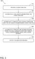
- FIG. 3 shows a flow chart for a method 300 for detecting regions of high curvature on a curve.
- Method 300 may be executed by one or more computing devices, such as processor 204 implementing one or more analysis applications, such as surface analysis application 226.
- curve functions may define at least a portion of an object surface.
- Object surface data corresponding to a 3D virtual model may be retrieved from a network-linked repository, such as non-volatile memory 208, storing 3D virtual models 210.
- method 300 includes receiving a curve function.
- the curve function may be extracted from one or more object surfaces.
- the curve function may be a single curve function derived from two or more boundaries extracted from adjacent pieces of the object surface.
- a 3D curve function may be projected into a 1D function by convolving the second derivative of the 3D curve function, and then by taking a dot product.
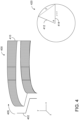
- FIG. 4 shows an example object surface 400.
- Object surface 400 may be a translation of a 2D curve function 402, as shown at 405.
- Object surface 400 includes an outer boundary 410, extending around the outside of object surface 400. Outer boundary 410 may be considered a group of edges of a plurality of object sheets that have been joined together.
- method 300 includes automatically arc length parameterizing the curve function.
- the curve function for object surface 400 may be parameterized to be the same as outer boundary 410. In this way, any point on the resultant function may be mapped to a point on object surface 400.
- arc length parameterizing the curve function results in the arc length parameterized curve function having constant speed.
- a curve function such as a spline can be represented as a parametric curve.
- Such a parametric curve may be arc-length parameterized by any suitable means.
- the parametric speed of the curve may be set such that movement over a fixed distance in parameter space yields movement of a fixed distance along the curve in physical space.
- the arc length parameterized curve function may have a constant parametric speed of 1.
- a new curve may be computed such that c : ⁇ ⁇ R 3 which is an approximation of f but is arc length parameterized.
- w L 2 .
- this problem may be illustrated by drawing the vectors c' ( s + w ) (412) and c' ( s - w ) (414) in the plane defined by the two 3D vectors, and we note that ⁇ c' ⁇ ⁇ 1 ⁇ ⁇ so the two vectors lie on the unit circle. This is shown at 420 in FIG. 4 .
- Trigonometry may then be applied to Equation 1 to express solutions in terms of the cosine of ⁇ .
- the arc length parametric curve may be subject to mathematical operations, such as derivatives, dot products, linear adjustments, hat functions, convolutions, etc.
- method 300 includes automatically computing local average curvature over the arc length parameterized curve function.
- automatically computing the local average curvature over the arc length parameterized curve function may comprise at least taking a dot product of the arc length parameterized curve function with itself.
- method 300 includes automatically indicating one or more regions where the local average curvature turns at least a predetermined angle over a given interval.
- the given interval may be in parameter space.
- Such a parameter space interval may correlate with a distance along the curve in model space.
- automatically indicating one or more regions where the local average curvature turns at least a predetermined angle ⁇ over a given interval L in parameter space comprises automatically identifying points where the arc length parameterized curve turns at the predetermined angle.
- Identifying such points may comprise generating solutions to the resulting function using a root finding solver.
- the curve function does not need to be convolved or integrated, as the goal is to determine where the derivative of the curve function has turned a certain number of degrees over a given interval.
- an equation of one variable ( s ) may be solved where c is the curve.
- the derivative may be taken at s - w and at s + w.
- the root finding problem can thus be solved where that dot product is equal to cos ⁇ .
- Such a problem may be solved via any number of numerical tools, such as the python numerical package or MATLAB.
- the root finding solver may derive roots that are equal to the zeros of Equation 6.
- c ′ s ⁇ w ⁇ c ′ s + w cos ⁇
- c' is the derivative of the arc length parameterized curve function
- s is an input variable of this function
- w is equal to half of the given interval
- ⁇ is the predetermined angle.
- automatically identifying points where the arc length parameterized curve turns at the predetermined angle may comprise automatically determining whether the interval between each neighboring pair of solutions is greater than or less than the given interval. As such, regions, not just points of high curvature may be determined. Such a formulation may be set to output any such points where the curve turns ⁇ ⁇ degrees over L inches.
- FIG. 5 shows an example plot 500 of Equation 6 representing object surface 400.
- C is the function
- xyz dependent variables
- s independent variable
- w is a constant (half the length of the interval of interest L) in parameter space. Because the curve function has been arc length parameterized to a function with a speed of 1, the interval L is also easily discernible in model space. Taking a dot product results in the dependent variables collapsing to a single output variable that is represented by plot 500, with a single input variable (s). As such, Equation 6 becomes a function with one input and one output.
- the solutions, or roots, where the local average curvature turns at least a predetermined angle ⁇ over a given interval L, are where plot 500 is equal to the cosine of the predetermined angle ⁇ (e.g., threshold 510). In practice, this yields a number of pairs of points (e.g., where curve crosses the threshold then crosses back).
- a more detailed view of a first set of points is shown at 520 (e.g., points 521-522, 523-524, 525-526, and 527-528) and a second set of points is shown in more detail at 530 531-532, 533-534, 535-536, and 537-538). Intervals between these pairs of points are indicated by bars.
- a more detailed view of a portion of plot 500 that indicates such intervals is shown at 540 (e.g., intervals 542, 544, 546, and 548).
- a range in parameter space is indicated for each region where the curvature is more than the predetermined ⁇ over interval L.
- a distance may be determined and compared to the predetermined interval L e.g., whether that interval has higher or lower curvature than the predetermined threshold.
- the function is parameterized as the boundary. As such, where the function passes cos ⁇ , the boundary starts. While four intervals (542, 544, 546, and 548) are shown, an additional four intervals (e.g., between pairs of points 531-532, 533-534, 535-536, and 537-538) also meet the criteria.
- FIG. 6 shows a view 600 of object surface 400 with intervals 542, 544, 546, and 548 overlaid.
- Inset 610 shows intervals 542, 544, 546, and 548 in greater detail.
- method 300 comprises outputting the indicated regions.
- the 4 points that have the highest curvature can be identified.
- the initial 3D curve can be converted to a function that is parameterized the same as the initial 3D curve, but features a single variable - e.g., the integrated curvature variable.
- the highest points of that function can be solved using any suitable approach for finding the critical points of a function. A user desiring four sides to a surface would thus solve for the four points of the function that have the highest values.
- Another challenge is to detect the corners of the object surface.
- the curve is convolved twice, and then squared. This approach allows for the determination of individual points where the function has the highest values. e.g., where the function is turning the most.
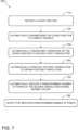
- FIG. 7 shows a flow-diagram for an example method 700 for detecting regions of maximal average curvature on a curve.
- Method 700 may be carried out by one or more computing devices, such as processor 204 implementing one or more analysis applications such as surface analysis application 226.
- curve functions may define at least a portion of an object surface.
- Object surface data corresponding to a 3D virtual model may be retrieved from a network-linked repository, such as non-volatile memory 208, storing 3D virtual models 210.
- method 700 comprises receiving a curve function.
- a curve function may define at least a portion of an object surface.
- the curve function can be represented with one or more splines.
- the curve function is a single curve function derived from two or more boundaries extracted from adjacent pieces of the object surface.
- FIG. 8 shows another depiction of object surface 400.
- C 2 discontinuities in the curve function may be automatically indicated based on detecting knot multiplicities.
- the C 2 discontinuities may be corrected by stitching adjacent splines or spline portions together and generating a single, continuous spline.
- the curve function can be chopped into C 2 continuous pieces, followed by checking the change in tangent angles at the discontinuities.
- it may be more effective to preprocess the curve function by convolving the curve function with a hat function.
- a curve function f may be preprocessed by convolving with a narrow hat function.
- ⁇ [-w/100.0, w /100.0] * f is used for preprocessing in some of the calculations shown below.
- method 700 comprises automatically parameterizing the curve function to a single variable.
- the single variable may be an integrated curvature variable.
- method 700 comprises automatically convolving a derivative of the curve function to obtain a first convolution.
- Equation 8 denotes an integral, this could also be represented as a convolution of c" with the hat function ⁇ [ -w,w ] . As such, convolution removes the need for large-scale integration of the curve function, thereby simplifying the calculation and reducing the processor load.
- method 700 comprises automatically convolving the first convolution to obtain a second convolution.
- the flat regions in the first convolution can be resolved by convolving a second time, generating single points near the center of the high average curvature regions. In other words, points where Equation 9 is maximized. ⁇ ⁇ w , w 2 2 w ⁇ c " s
- Plot 800 is an example of Equation 9 as applied to object surface 400.
- Four points of highest average curvature are shown at 802, 804, 806, and 808.
- Four additional points of high average curvature are shown at 812, 814, 816, and 818. Any point of high curvature will show as a spike.
- method 700 comprises automatically indicating a predetermined number of points of the second convolution having maximal values.
- the predetermined number of points of the second convolution having maximal values are automatically indicated using a root finding solver for Eq. 10.
- the predetermined number of points may be input by a user, selected based on characteristics of the curve function, determined by thresholding the second convolution etc.
- the indicated predetermined number of points may represent single points near centers of regions of maximal average curvature on the object surface.
- object surface 400 may be characterized by four critical points or corners (e.g., 802, 808, 812, 818).
- Four other points of interest e.g., 804, 806, 814, 816) also show maximal average curvature, and are the points which next most resemble corners.
- the threshold may be applied to a specific region of the univariate function (e.g., to indicate corners of one portion of the object surface).
- method 700 comprises outputting the indicated predetermined number of points.
- Arc length parameterization allows the curvature of an object surface to be treated as a set of second derivatives. This reduces computational complexity, allowing the curves to be reasoned about in a mathematical library.
- the systems and methods described herein further have the potential benefits of reducing the need for human interaction and input during the analysis process.
- the methods described herein enable progress towards a larger goal of seamlessly integrating analysis tools which operate on single-cell geometry with design software that store models as multi-piece designs.
- regions of high curvature and points of maximal average curvature can be used in various applications.
- the regions of high curvature and points of maximal average curvature can be used in additive manufacturing applications, for example, to optimize the weight, cost, and/or function of a 3D manufactured object through 3D model modifications.
- the regions of high curvature and points of maximal average curvature can also be used to more accurately characterize the geometry of a part of surface. For example, unexpected, short-distance regions of high angle curvature may be revealed.
- the surface analysis software can then be programmed to excise those portions, and stitch in a smoother, or less angular, portion into the model.
- the processes described herein may further be used to generate indications of curve quality. For examples, object surfaces can be inspected to ensure they have sufficient smoothness for their intended purpose.
- the surface of aircraft model 100 or a component thereof, such as wing region 104 can be the object surface that is used for detecting regions of high curvature and/or maximal average curvature by the 3D virtual model 210 in accordance with the system 200 and methods 300 and 700 of the subject disclosure.
- system 200 and methods 300 and 700 can be useful for any application that analyzes surfaces of geometric parts and encounters scenarios where there is utility in reasoning about where corners and sharp turns are located on the boundary of such surfaces.
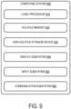
- FIG. 9 illustrates an exemplary computing system 900 that can be utilized to implement the system 200 and methods 300 and 700 described above.
- Computing system 900 includes a logic processor 910, volatile memory 920, and a non-volatile storage device 930.
- Computing system 900 can optionally include a display subsystem 940, input subsystem 950, communication subsystem 960 connected to a computer network, and/or other components not shown in FIG. 9 . These components are typically connected for data exchange by one or more data buses when integrated into single device, or by a combination of data buses, network data interfaces, and computer networks when integrated into separate devices connected by computer networks.
- the non-volatile storage device 930 stores various instructions, also referred to as software, which are executed by the logic processor 910.
- Logic processor 910 includes one or more physical devices configured to execute the instructions.
- the logic processor 910 can be configured to execute instructions that are part of one or more applications, programs, routines, libraries, objects, components, data structures, or other logical constructs. Such instructions can be implemented to perform a task, implement a data type, transform the state of one or more components, achieve a technical effect, or otherwise arrive at a desired result.
- the logic processor 910 can include one or more physical processors (hardware) configured to execute software instructions. Additionally or alternatively, the logic processor 910 can include one or more hardware logic circuits or firmware devices configured to execute hardware-implemented logic or firmware instructions. Processors of the logic processor 910 can be single-core or multi-core, and the instructions executed thereon can be configured for sequential, parallel, and/or distributed processing. Individual components of the logic processor 910 optionally can be distributed among two or more separate devices, which can be remotely located and/or configured for coordinated processing. Aspects of the logic processor 910 can be virtualized and executed by remotely accessible, networked computing devices configured in a cloud-computing configuration. In such a case, these virtualized aspects are run on different physical logic processors of various different machines, it will be understood.
- Non-volatile storage device 930 includes one or more physical devices configured to hold instructions executable by the logic processors to implement the methods and processes described herein. When such methods and processes are implemented, the state of non-volatile storage device 930 can be transformed-e.g., to hold different data.
- Non-volatile storage device 930 can include physical devices that are removable and/or built-in.
- Non-volatile storage device 930 can include optical memory (e.g., CD, DVD, HD-DVD, Blu-Ray Disc, etc.), semiconductor memory (e.g., ROM, EPROM, EEPROM, FLASH memory, etc.), and/or magnetic memory (e.g., hard-disk drive, floppy-disk drive, tape drive, MRAM, etc.), or other mass storage device technology.
- Non-volatile storage device 930 can include nonvolatile, dynamic, static, read/write, read-only, sequential-access, location-addressable, file-addressable, and/or content-addressable devices. It will be appreciated that non-volatile storage device 930 is configured to hold instructions even when power is cut to the non-volatile storage device 930.
- Volatile memory 920 can include physical devices that include random access memory. Volatile memory 920 is typically utilized by logic processor 910 to temporarily store information during processing of software instructions. It will be appreciated that volatile memory 920 typically does not continue to store instructions when power is cut to the volatile memory 920.
- logic processor 910 volatile memory 920, and non-volatile storage device 930 can be integrated together into one or more hardware-logic components.
- hardware-logic components can include field-programmable gate arrays (FPGAs), program- and application-specific integrated circuits (PASIC / ASICs), program- and application-specific standard products (PSSP / ASSPs), system-on-a-chip (SOC), and complex programmable logic devices (CPLDs), for example.
- FPGAs field-programmable gate arrays
- PASIC / ASICs program- and application-specific integrated circuits
- PSSP / ASSPs program- and application-specific standard products
- SOC system-on-a-chip
- CPLDs complex programmable logic devices
- module can be used to describe an aspect of the surface analysis system 200 typically implemented in software by a processor to perform a particular function using portions of volatile memory, which function involves transformative processing that specially configures the processor to perform the function.
- a module, program, or engine can be instantiated via logic processor 910 executing instructions held by non-volatile storage device 930, using portions of volatile memory 920.
- modules, programs, and/or engines can be instantiated from the same application, service, code block, object, library, routine, API, function, etc.
- the same module, program, and/or engine can be instantiated by different applications, services, code blocks, objects, routines, APIs, functions, etc.
- module can encompass individual or groups of executable files, data files, libraries, drivers, scripts, database records, etc.
- Display subsystem 940 typically includes one or more displays, which can be physically integrated with or remote from a device that houses the logic processor 910. Graphical output of the logic processor executing the instructions described above, such as a graphical user interface, is configured to be displayed on display subsystem 940.
- Input subsystem 950 typically includes one or more of a keyboard, pointing device (e.g., mouse, trackpad, finger operated pointer), touchscreen, microphone, and camera. Other input devices can also be provided.
- Communication subsystem 960 is configured to communicatively couple various computing devices described herein with each other, and with other devices.
- Communication subsystem 960 can include wired and/or wireless communication devices compatible with one or more different communication protocols.
- the communication subsystem can be configured for communication via a wireless telephone network, or a wired or wireless local- or wide-area network by devices such as a 3G, 4G, 5G, or 6G radio, Wi-Fi card, Ethernet network interface card, BLUETOOTH radio, etc.
- the communication subsystem can allow computing system 900 to send and/or receive messages to and/or from other devices via a network such as the Internet.
- one or more of the computer networks via which communication subsystem 960 is configured to communicate can include security measures such as user identification and authentication, access control, malware detection, enforced encryption, content filtering, etc., and can be coupled to a wide area network (WAN) such as the Internet.
- security measures such as user identification and authentication, access control, malware detection, enforced encryption, content filtering, etc.
- WAN wide area network
- the subject disclosure includes all novel and non-obvious combinations and subcombinations of the various features and techniques disclosed herein.
- the various features and techniques disclosed herein are not necessarily required of all examples of the subject disclosure.
- the various features and techniques disclosed herein can define patentable subject matter apart from the disclosed examples and can find utility in other implementations not expressly disclosed herein.
- a method for detecting regions of high curvature on a curve comprising receiving a curve function; automatically arc length parameterizing the curve function; automatically computing local average curvature over the arc length parameterized curve function; automatically indicating one or more regions where the local average curvature turns at least a predetermined angle over a given interval; and outputting the indicated regions.
- Clause 7 The method of any of clauses 1-6, wherein automatically identifying points where the arc length parameterized curve turns at the predetermined angle is performed by a root finding solver.
- a method for detecting regions of maximal average curvature on a curve comprising receiving a curve function; automatically parameterizing the curve function to a single variable; automatically convolving a derivative of the curve function to obtain a first convolution; automatically convolving the first convolution to obtain a second convolution; automatically indicating a predetermined number of points of the second convolution having maximal values; and outputting the indicated predetermined number of points.
- Clause 11 The method of clause 9 or 10, wherein the indicated predetermined number of points represent single points near centers of regions of maximal average curvature on the object surface.
- Clause 12 The method of any of clauses 9-11, wherein the predetermined number of points of the second convolution having maximal values are automatically indicated using a root finding solver.
- Clause 14 The method of any of clauses 9-13, wherein the method further comprises automatically indicating discontinuities in the curve function based on detecting knot multiplicities.
- Clause 15 The method of any of clauses 9-14, wherein the method further comprises preprocessing the curve function by convolving the curve function with a hat function.
- a surface analysis system comprising at least one processor, communicatively coupled to non-volatile memory storing a three-dimensional (3D) virtual model and instructions that, when executed by the processor, cause the processor to receive a curve function defining a portion of an object surface; automatically arc length parameterize the curve function; automatically compute local average curvature over the arc length parameterized curve function; automatically indicate one or more regions where the local average curvature turns at least a predetermined angle over a given interval in parameter space; and output the indicated regions.
- 3D three-dimensional
- Clause 18 The surface analysis system of clause 17, wherein automatically indicating one or more regions where the local average curvature turns at least a predetermined angle over a given interval in parameter space comprises automatically identifying points where the arc length parameterized curve turns at the predetermined angle; and automatically determining whether the interval between each neighboring pair of solutions is greater than or less than the given interval.
- non-volatile memory further stores instructions that, when executed by the processor, cause the processor to receive a curve function defining at least a portion of the object surface; automatically parameterize the curve function to a single variable; automatically convolve a derivative of the curve function to obtain a first convolution; automatically convolve the first convolution to obtain a second convolution; automatically indicate a predetermined number of points of the second convolution having maximal values; and output the indicated predetermined number of points.
Landscapes
- Engineering & Computer Science (AREA)
- Physics & Mathematics (AREA)
- General Physics & Mathematics (AREA)
- Theoretical Computer Science (AREA)
- Geometry (AREA)
- Mathematical Optimization (AREA)
- Mathematical Analysis (AREA)
- Pure & Applied Mathematics (AREA)
- Computational Mathematics (AREA)
- General Engineering & Computer Science (AREA)
- Mathematical Physics (AREA)
- Software Systems (AREA)
- Computer Hardware Design (AREA)
- Data Mining & Analysis (AREA)
- Evolutionary Computation (AREA)
- Algebra (AREA)
- Aviation & Aerospace Engineering (AREA)
- Automation & Control Theory (AREA)
- Databases & Information Systems (AREA)
- Operations Research (AREA)
- Computing Systems (AREA)
- Computer Graphics (AREA)
- Image Analysis (AREA)
- Image Generation (AREA)
- Length Measuring Devices With Unspecified Measuring Means (AREA)
Applications Claiming Priority (1)
| Application Number | Priority Date | Filing Date | Title |
|---|---|---|---|
| US18/313,221 US12340218B2 (en) | 2023-05-05 | 2023-05-05 | Detection of high curvature regions on curves |
Publications (2)
| Publication Number | Publication Date |
|---|---|
| EP4459495A2 true EP4459495A2 (de) | 2024-11-06 |
| EP4459495A3 EP4459495A3 (de) | 2025-01-08 |
Family
ID=91027119
Family Applications (1)
| Application Number | Title | Priority Date | Filing Date |
|---|---|---|---|
| EP24174221.2A Pending EP4459495A3 (de) | 2023-05-05 | 2024-05-03 | Erkennung von bereichen mit hoher krümmung auf kurven |
Country Status (3)
| Country | Link |
|---|---|
| US (1) | US12340218B2 (de) |
| EP (1) | EP4459495A3 (de) |
| CN (1) | CN118898111A (de) |
Family Cites Families (4)
| Publication number | Priority date | Publication date | Assignee | Title |
|---|---|---|---|---|
| WO2015083009A1 (en) * | 2013-12-04 | 2015-06-11 | Mobileye Vision Technologies Ltd. | Systems and methods for mimicking a leading vehicle |
| US11880980B2 (en) * | 2016-06-17 | 2024-01-23 | Children's National Medical Center | Medical anatomy quantification: computer-aided diagnosis tool |
| US12012220B2 (en) | 2021-02-11 | 2024-06-18 | The Boeing Company | Calibration system and method for aircraft control surface actuation |
| US12325445B2 (en) * | 2022-05-31 | 2025-06-10 | Korea Advanced Institute Of Science And Technology | High-definition map-based local path planning method and apparatus for dynamic and static obstacle avoidance |
-
2023
- 2023-05-05 US US18/313,221 patent/US12340218B2/en active Active
-
2024
- 2024-04-22 CN CN202410480872.6A patent/CN118898111A/zh active Pending
- 2024-05-03 EP EP24174221.2A patent/EP4459495A3/de active Pending
Also Published As
| Publication number | Publication date |
|---|---|
| CN118898111A (zh) | 2024-11-05 |
| US20240370259A1 (en) | 2024-11-07 |
| EP4459495A3 (de) | 2025-01-08 |
| US12340218B2 (en) | 2025-06-24 |
Similar Documents
| Publication | Publication Date | Title |
|---|---|---|
| US20230360320A1 (en) | Inserting three-dimensional objects into digital images with consistent lighting via global and local lighting information | |
| Hummel et al. | Comparative visual analysis of Lagrangian transport in CFD ensembles | |
| EP3321817B1 (de) | Abfrage einer datenbank auf basis einer parametrischen ansichtsfunktion | |
| CN110325327A (zh) | 用于保护基于云的制造分析服务的隐私的方法和系统 | |
| Wang et al. | Fast iterative region inflation for computing large 2-d/3-d convex regions of obstacle-free space | |
| US20140067333A1 (en) | CAD-Based System for Product Definition, Inspection and Validation | |
| Bründl et al. | Semantic part segmentation of spatial features via geometric deep learning for automated control cabinet assembly | |
| Raj Prasanth et al. | Collision detection during planning for sheet metal bending by bounding volume hierarchy approaches | |
| Gajamannage et al. | Dimensionality reduction of collective motion by principal manifolds | |
| Jiang et al. | Efficient Booleans algorithms for triangulated meshes of geometric modeling | |
| US12340218B2 (en) | Detection of high curvature regions on curves | |
| US20160267352A1 (en) | System and method for constructing a statistical shape model | |
| Bokovoy et al. | Map-merging algorithms for visual slam: Feasibility study and empirical evaluation | |
| Ventura et al. | Surface intersection in geometric modeling of ship hulls | |
| de Carvalho et al. | Improving knn classification under unbalanced data. A new geometric oversampling approach | |
| Li et al. | An algorithm for filling complex holes in reverse engineering | |
| Luo et al. | Optimal tool orientation generation and chip volume/cutting force predictions for 5-axis CNC machining of curved surfaces using flat-end mills | |
| Shimshoni et al. | Probabilistic 3d object recognition | |
| US8289332B2 (en) | Apparatus and method for determining intersections | |
| Lee et al. | Facial landmark detection using Gaussian guided regression network | |
| Vršek et al. | Reducibility of offsets to algebraic curves | |
| Wang | Research on Shape Feature Recognition of B‐Rep Model Based on Wavelet Transform | |
| Kim et al. | Practical method for the fast generation of a CAM model for jet engine parts | |
| Li et al. | An analysis-oriented parameter extraction method for features on freeform surface | |
| Lin et al. | Orthogonal integral transform for 3D shape recognition with few examples |
Legal Events
| Date | Code | Title | Description |
|---|---|---|---|
| PUAI | Public reference made under article 153(3) epc to a published international application that has entered the european phase |
Free format text: ORIGINAL CODE: 0009012 |
|
| STAA | Information on the status of an ep patent application or granted ep patent |
Free format text: STATUS: THE APPLICATION HAS BEEN PUBLISHED |
|
| AK | Designated contracting states |
Kind code of ref document: A2 Designated state(s): AL AT BE BG CH CY CZ DE DK EE ES FI FR GB GR HR HU IE IS IT LI LT LU LV MC ME MK MT NL NO PL PT RO RS SE SI SK SM TR |
|
| PUAL | Search report despatched |
Free format text: ORIGINAL CODE: 0009013 |
|
| AK | Designated contracting states |
Kind code of ref document: A3 Designated state(s): AL AT BE BG CH CY CZ DE DK EE ES FI FR GB GR HR HU IE IS IT LI LT LU LV MC ME MK MT NL NO PL PT RO RS SE SI SK SM TR |
|
| RIC1 | Information provided on ipc code assigned before grant |
Ipc: G06T 17/30 20060101ALI20241204BHEP Ipc: G06F 30/17 20200101ALI20241204BHEP Ipc: G06F 30/15 20200101AFI20241204BHEP |
|
| STAA | Information on the status of an ep patent application or granted ep patent |
Free format text: STATUS: REQUEST FOR EXAMINATION WAS MADE |
|
| 17P | Request for examination filed |
Effective date: 20250627 |
|
| STAA | Information on the status of an ep patent application or granted ep patent |
Free format text: STATUS: EXAMINATION IS IN PROGRESS |
|
| 17Q | First examination report despatched |
Effective date: 20251001 |
|
| GRAP | Despatch of communication of intention to grant a patent |
Free format text: ORIGINAL CODE: EPIDOSNIGR1 |
|
| STAA | Information on the status of an ep patent application or granted ep patent |
Free format text: STATUS: GRANT OF PATENT IS INTENDED |
|
| INTG | Intention to grant announced |
Effective date: 20260223 |
|
| GRAS | Grant fee paid |
Free format text: ORIGINAL CODE: EPIDOSNIGR3 |