EP4450925A1 - Localizing a moving vehicle - Google Patents

Localizing a moving vehicle Download PDF

Info

Publication number
EP4450925A1
EP4450925A1 EP23169054.6A EP23169054A EP4450925A1 EP 4450925 A1 EP4450925 A1 EP 4450925A1 EP 23169054 A EP23169054 A EP 23169054A EP 4450925 A1 EP4450925 A1 EP 4450925A1
Authority
EP
European Patent Office
Prior art keywords
gnss
vehicle
data
odometer
predicted
Prior art date
Legal status (The legal status is an assumption and is not a legal conclusion. Google has not performed a legal analysis and makes no representation as to the accuracy of the status listed.)
Pending
Application number
EP23169054.6A
Other languages
German (de)
French (fr)
Inventor
Mohamed Radwan
Alaaeldin ZAKY
Current Assignee (The listed assignees may be inaccurate. Google has not performed a legal analysis and makes no representation or warranty as to the accuracy of the list.)
Valeo Comfort and Driving Assistance SAS
Original Assignee
Valeo Comfort and Driving Assistance SAS
Priority date (The priority date is an assumption and is not a legal conclusion. Google has not performed a legal analysis and makes no representation as to the accuracy of the date listed.)
Filing date
Publication date
Application filed by Valeo Comfort and Driving Assistance SAS filed Critical Valeo Comfort and Driving Assistance SAS
Priority to EP23169054.6A priority Critical patent/EP4450925A1/en
Priority to US18/641,112 priority patent/US20240353578A1/en
Priority to CN202410481467.6A priority patent/CN118816856A/en
Publication of EP4450925A1 publication Critical patent/EP4450925A1/en
Pending legal-status Critical Current

Links

Images

Classifications

    • GPHYSICS
    • G01MEASURING; TESTING
    • G01SRADIO DIRECTION-FINDING; RADIO NAVIGATION; DETERMINING DISTANCE OR VELOCITY BY USE OF RADIO WAVES; LOCATING OR PRESENCE-DETECTING BY USE OF THE REFLECTION OR RERADIATION OF RADIO WAVES; ANALOGOUS ARRANGEMENTS USING OTHER WAVES
    • G01S19/00Satellite radio beacon positioning systems; Determining position, velocity or attitude using signals transmitted by such systems
    • G01S19/38Determining a navigation solution using signals transmitted by a satellite radio beacon positioning system
    • G01S19/39Determining a navigation solution using signals transmitted by a satellite radio beacon positioning system the satellite radio beacon positioning system transmitting time-stamped messages, e.g. GPS [Global Positioning System], GLONASS [Global Orbiting Navigation Satellite System] or GALILEO
    • G01S19/42Determining position
    • G01S19/48Determining position by combining or switching between position solutions derived from the satellite radio beacon positioning system and position solutions derived from a further system
    • G01S19/49Determining position by combining or switching between position solutions derived from the satellite radio beacon positioning system and position solutions derived from a further system whereby the further system is an inertial position system, e.g. loosely-coupled
    • GPHYSICS
    • G01MEASURING; TESTING
    • G01CMEASURING DISTANCES, LEVELS OR BEARINGS; SURVEYING; NAVIGATION; GYROSCOPIC INSTRUMENTS; PHOTOGRAMMETRY OR VIDEOGRAMMETRY
    • G01C21/00Navigation; Navigational instruments not provided for in groups G01C1/00 - G01C19/00
    • G01C21/10Navigation; Navigational instruments not provided for in groups G01C1/00 - G01C19/00 by using measurements of speed or acceleration
    • G01C21/12Navigation; Navigational instruments not provided for in groups G01C1/00 - G01C19/00 by using measurements of speed or acceleration executed aboard the object being navigated; Dead reckoning
    • G01C21/16Navigation; Navigational instruments not provided for in groups G01C1/00 - G01C19/00 by using measurements of speed or acceleration executed aboard the object being navigated; Dead reckoning by integrating acceleration or speed, i.e. inertial navigation
    • G01C21/165Navigation; Navigational instruments not provided for in groups G01C1/00 - G01C19/00 by using measurements of speed or acceleration executed aboard the object being navigated; Dead reckoning by integrating acceleration or speed, i.e. inertial navigation combined with non-inertial navigation instruments
    • GPHYSICS
    • G01MEASURING; TESTING
    • G01CMEASURING DISTANCES, LEVELS OR BEARINGS; SURVEYING; NAVIGATION; GYROSCOPIC INSTRUMENTS; PHOTOGRAMMETRY OR VIDEOGRAMMETRY
    • G01C21/00Navigation; Navigational instruments not provided for in groups G01C1/00 - G01C19/00
    • G01C21/10Navigation; Navigational instruments not provided for in groups G01C1/00 - G01C19/00 by using measurements of speed or acceleration
    • G01C21/12Navigation; Navigational instruments not provided for in groups G01C1/00 - G01C19/00 by using measurements of speed or acceleration executed aboard the object being navigated; Dead reckoning
    • G01C21/16Navigation; Navigational instruments not provided for in groups G01C1/00 - G01C19/00 by using measurements of speed or acceleration executed aboard the object being navigated; Dead reckoning by integrating acceleration or speed, i.e. inertial navigation
    • G01C21/165Navigation; Navigational instruments not provided for in groups G01C1/00 - G01C19/00 by using measurements of speed or acceleration executed aboard the object being navigated; Dead reckoning by integrating acceleration or speed, i.e. inertial navigation combined with non-inertial navigation instruments
    • G01C21/1652Navigation; Navigational instruments not provided for in groups G01C1/00 - G01C19/00 by using measurements of speed or acceleration executed aboard the object being navigated; Dead reckoning by integrating acceleration or speed, i.e. inertial navigation combined with non-inertial navigation instruments with ranging devices, e.g. LIDAR or RADAR
    • GPHYSICS
    • G01MEASURING; TESTING
    • G01CMEASURING DISTANCES, LEVELS OR BEARINGS; SURVEYING; NAVIGATION; GYROSCOPIC INSTRUMENTS; PHOTOGRAMMETRY OR VIDEOGRAMMETRY
    • G01C21/00Navigation; Navigational instruments not provided for in groups G01C1/00 - G01C19/00
    • G01C21/10Navigation; Navigational instruments not provided for in groups G01C1/00 - G01C19/00 by using measurements of speed or acceleration
    • G01C21/12Navigation; Navigational instruments not provided for in groups G01C1/00 - G01C19/00 by using measurements of speed or acceleration executed aboard the object being navigated; Dead reckoning
    • G01C21/16Navigation; Navigational instruments not provided for in groups G01C1/00 - G01C19/00 by using measurements of speed or acceleration executed aboard the object being navigated; Dead reckoning by integrating acceleration or speed, i.e. inertial navigation
    • G01C21/183Compensation of inertial measurements, e.g. for temperature effects
    • G01C21/188Compensation of inertial measurements, e.g. for temperature effects for accumulated errors, e.g. by coupling inertial systems with absolute positioning systems
    • GPHYSICS
    • G01MEASURING; TESTING
    • G01CMEASURING DISTANCES, LEVELS OR BEARINGS; SURVEYING; NAVIGATION; GYROSCOPIC INSTRUMENTS; PHOTOGRAMMETRY OR VIDEOGRAMMETRY
    • G01C25/00Manufacturing, calibrating, cleaning, or repairing instruments or devices referred to in the other groups of this subclass
    • GPHYSICS
    • G01MEASURING; TESTING
    • G01SRADIO DIRECTION-FINDING; RADIO NAVIGATION; DETERMINING DISTANCE OR VELOCITY BY USE OF RADIO WAVES; LOCATING OR PRESENCE-DETECTING BY USE OF THE REFLECTION OR RERADIATION OF RADIO WAVES; ANALOGOUS ARRANGEMENTS USING OTHER WAVES
    • G01S19/00Satellite radio beacon positioning systems; Determining position, velocity or attitude using signals transmitted by such systems
    • G01S19/38Determining a navigation solution using signals transmitted by a satellite radio beacon positioning system
    • G01S19/39Determining a navigation solution using signals transmitted by a satellite radio beacon positioning system the satellite radio beacon positioning system transmitting time-stamped messages, e.g. GPS [Global Positioning System], GLONASS [Global Orbiting Navigation Satellite System] or GALILEO
    • G01S19/393Trajectory determination or predictive tracking, e.g. Kalman filtering
    • GPHYSICS
    • G01MEASURING; TESTING
    • G01SRADIO DIRECTION-FINDING; RADIO NAVIGATION; DETERMINING DISTANCE OR VELOCITY BY USE OF RADIO WAVES; LOCATING OR PRESENCE-DETECTING BY USE OF THE REFLECTION OR RERADIATION OF RADIO WAVES; ANALOGOUS ARRANGEMENTS USING OTHER WAVES
    • G01S19/00Satellite radio beacon positioning systems; Determining position, velocity or attitude using signals transmitted by such systems
    • G01S19/38Determining a navigation solution using signals transmitted by a satellite radio beacon positioning system
    • G01S19/39Determining a navigation solution using signals transmitted by a satellite radio beacon positioning system the satellite radio beacon positioning system transmitting time-stamped messages, e.g. GPS [Global Positioning System], GLONASS [Global Orbiting Navigation Satellite System] or GALILEO
    • G01S19/42Determining position
    • G01S19/45Determining position by combining measurements of signals from the satellite radio beacon positioning system with a supplementary measurement
    • GPHYSICS
    • G01MEASURING; TESTING
    • G01SRADIO DIRECTION-FINDING; RADIO NAVIGATION; DETERMINING DISTANCE OR VELOCITY BY USE OF RADIO WAVES; LOCATING OR PRESENCE-DETECTING BY USE OF THE REFLECTION OR RERADIATION OF RADIO WAVES; ANALOGOUS ARRANGEMENTS USING OTHER WAVES
    • G01S19/00Satellite radio beacon positioning systems; Determining position, velocity or attitude using signals transmitted by such systems
    • G01S19/38Determining a navigation solution using signals transmitted by a satellite radio beacon positioning system
    • G01S19/39Determining a navigation solution using signals transmitted by a satellite radio beacon positioning system the satellite radio beacon positioning system transmitting time-stamped messages, e.g. GPS [Global Positioning System], GLONASS [Global Orbiting Navigation Satellite System] or GALILEO
    • G01S19/42Determining position
    • G01S19/45Determining position by combining measurements of signals from the satellite radio beacon positioning system with a supplementary measurement
    • G01S19/47Determining position by combining measurements of signals from the satellite radio beacon positioning system with a supplementary measurement the supplementary measurement being an inertial measurement, e.g. tightly coupled inertial

Definitions

  • the disclosure relates to the field of computer programs and systems, and more specifically to a method, system and program for localization of a moving vehicle.
  • a number of systems and programs are offered on the market for tracking the localization of a vehicle.
  • the method comprises, in real-time, obtaining vehicle motion data.
  • the vehicle motion data stems from at least one vehicle sensor.
  • the method also comprises, in real-time, obtaining, while the GNSS signal is available, GNSS data of a positioning of the vehicle.
  • the GNSS data includes a distance variation and an orientation variation.
  • the method also comprises, in real-time, calibrating parameters of an odometer of the vehicle.
  • the calibration is based on a data fusion that uses a Kalman filter.
  • the Kalman filter determines a predicted distance variation and a predicted orientation variation of the vehicle based on a current calibration of the odometer parameters and on the motion data.
  • the Kalman filter also compares the predicted distance variation and predicted orientation variation to the distance variation and the orientation variation of the GNSS data.
  • the method may comprise one or more of the following:
  • a system comprising a processor coupled to a memory, the memory having recorded thereon the computer program.
  • the system may comprise one or more of the following:
  • the method comprises, in real-time, obtaining vehicle motion data.
  • the vehicle motion data stems from at least one vehicle sensor.
  • the method also comprises, in real-time, obtaining, while the GNSS signal is available, GNSS data of a positioning of the vehicle.
  • the GNSS data includes a distance variation and an orientation variation.
  • the method also comprises, in real-time, calibrating parameters of an odometer of the vehicle. The calibration is based on a data fusion that uses a Kalman filter.
  • the Kalman filter determines a predicted distance variation and a predicted orientation variation of the vehicle based on a current calibration of the odometer parameters and on the motion data.
  • the Kalman filter also compares the predicted distance variation and predicted orientation variation to the distance variation and the orientation variation of the GNSS data.
  • Such a method improves the localization of the moving vehicle.
  • the method achieves an improved accuracy for localizing the moving vehicle regardless of where the vehicle may be spatially localized, for example, regardless of whether the vehicle is localized inside a tunnel or in an open field.
  • vehicle motion data consists on local data which is acquired from the at least one vehicle sensor (for example comprising a wheel sensor, an Inertial Measurement Unit (IMU), and a steering system sensor) and thus provides data about the vehicle motion.
  • vehicle sensor for example comprising a wheel sensor, an Inertial Measurement Unit (IMU), and a steering system sensor
  • the GNSS data provides an accurate data of positioning of the vehicle (including GNSS motion data such as the distance variation and the orientation variation) while the GNSS signal is available, for example, in an open field covered by GPS coverture (which is the case during the majority of the vehicle's trip, except on short periods where the vehicle goes through a tunnel or the like).
  • the vehicle motion data on its own is sensible to sensor-related errors.
  • the speed obtained from a sensor such as a wheel encoder may be based on a default tire size (wheel circumference), which could vary due to change of tire pressure/temperature or exchanging the tires with others with different circumference like the summer/winter exchange. Such change in the tire size may introduce scaling factor error in the measured speed.
  • a sensor such as an IMU provides angular speeds and acceleration for yaw, pitch, and roll based on builtin gyroscope.
  • the readings of such electro-mechanical sensor may be highly affected by significant temperature/pressure changes, and a slight shift in the mounting of the sensor shall introduce bias error to it.
  • a sensor such as a steering system sensor is based on feeding back the place of the slider on the steering rack to indicate the steering measurement, which may present offset errors due to its mechanical sliding resolution.
  • the Odometer sensors scaling and offset errors may be dynamically changing, and the present method may estimate them continuously in order to locate the vehicle accurately.
  • the method also relies also on the GNSS data, the method re-calibrates the odometer using the GNSS data, which is known to be particularly reliable, so as to compensate for such errors.
  • the method further improves the robustness for localizing the vehicle based on both the vehicle motion data and the GNSS data.
  • the odometer (providing information on the motion of the vehicle) may be subject to changes in pressure and/or temperature which may introduce error factors in the vehicle motion data stemming from the at least one sensor.
  • the method determines a predicted distance variation and a predicted orientation variation based on a data fusion of the GNSS and sensor data so that the method corrects parameters of the odometer based on the comparison of the predicted ( i . e .
  • the calibration is also done relatively continuously (e.g., continuously while the GNSS signal is available, e.g. at regular and short time intervals/steps) and thus the odometer is persistently calibrated as the comparison is done every time there is a track (that is, a distance traveled by the vehicle) that can be extracted from both the odometer and GNSS data, for example where there is suitable coverage from a GNSS system such as satellites.
  • the calibrated odometer upon losing the GNSS data, the calibrated odometer, which is conform to the last available GNSS data, makes on its own accurate prediction using the calibrated parameters during the absence of the GNSS data.
  • the odometer is continuously/in real-time calibrated and the vehicle localization can be determined based on the calibrated odometer and on the GNSS and sensor data.
  • the method is computer-implemented. This means that steps (or substantially all the steps) of the method are executed by at least one computer, or any system alike. Thus, steps of the method are performed by the computer, possibly fully automatically, or, semi-automatically. In examples, the triggering of at least some of the steps of the method may be performed through user-computer interaction.
  • the level of user-computer interaction required may depend on the level of automatism foreseen and put in balance with the need to implement user's wishes. In examples, this level may be user-defined and/or pre-defined.
  • a typical example of computer-implementation of a method is to perform the method with a system adapted for this purpose.
  • the system may comprise a processor coupled to a memory and a graphical user interface (GUI), the memory having recorded thereon a computer program comprising instructions for performing the method.
  • GUI graphical user interface
  • the memory may also store a database.
  • the memory is any hardware adapted for such storage, possibly comprising several physical distinct parts (e.g. one for the program, and possibly one for the database).
  • the system may be coupled or further comprise the GNSS device, the odometer, and the at least one sensor.
  • the at least one sensor may include a wheel sensor, an Inertial Measurement Unit (IMU), and a steering system sensor.
  • IMU Inertial Measurement Unit
  • FIG. 1 shows an example of the system, wherein the system is a computer system 100 configured to be mounted on a vehicle.
  • the computer 100 of the example comprises a processor or processing unit such as a central processing unit (CPU) 1010 connected to an internal communication BUS 1000.
  • a random access memory (RAM) may be optionally connected to the BUS (not shown).
  • a memory controller 1020 manages accesses to a mass memory device, such as hard drive or other form of non-volatile memory such as EPROM, EEPROM, and flash memory devices. Any of the foregoing may be supplemented by, or incorporated in, specially designed ASICs (application-specific integrated circuits).
  • the computer may optionally also include a display, e.g., a touch screen (not shown). The display may be configured for displaying the localization of the vehicle.
  • the computer 100 may be coupled with a GNSS 1080 through a port or interface 1090 and with a wheel sensor 1050 like a wheel encoder, an IMU 1040 and a steering system sensor 1030 through a port or interface 1060.
  • the computer 100 may comprise an output port 1070 for sending calibration parameters to the odometer 1110.
  • the computer 100 may also comprise an output port 1100 for outputting the data forming the vehicle's predicted localization.
  • the odometer 1110 may be coupled with the computer 100 as shown in the figure to send its predictions to the computer.
  • the data may comprise the localization and the heading of the vehicle and any other localization data discussed herein.
  • the display may also be configured for displaying the localization of the vehicle.
  • the computer program may comprise instructions executable by a computer, the instructions comprising means for causing the above system to perform the method.
  • the program may be recordable on any data storage medium, including the memory of the system.
  • the program may for example be implemented in digital electronic circuitry, or in computer hardware, firmware, software, or in combinations of them.
  • the program may be implemented as an apparatus, for example a product tangibly embodied in a machine-readable storage device for execution by a programmable processor. Method steps may be performed by a programmable processor executing a program of instructions to perform functions of the method by operating on input data and generating output.
  • the processor may thus be programmable and coupled to receive data and instructions from, and to transmit data and instructions to, a data storage system, at least one input device, and at least one output device.
  • the application program may be implemented in a high-level procedural or object-oriented programming language, or in assembly or machine language if desired. In any case, the language may be a compiled or interpreted language.
  • the program may be a full installation program or an update program. Application of the program on the system results in any case in instructions for performing the method.
  • the computer program may alternatively be stored and executed on a server of a cloud computing environment, the server being in communication across a network with one or more clients. In such a case a processing unit executes the instructions comprised by the program, thereby causing the method to be performed on the cloud computing environment.
  • the vehicle may be a motorbike, a car, a bus or a truck.
  • the method is for determining the localization of the moving vehicle, that is, the spatial location of the vehicle as it follows a generally continuous movement (this does however not exclude vehicle stops, for example at red lights).
  • the localization may be expressed in terms of the 3D cartesian coordinates (x,y,z) with z denoting (by convention) an altitude of the vehicle with respect to the x-y plane or 2D cartesian coordinates (x,y), by considering the projection of the vehicle to the ground in the x-y plane.
  • the method may output the localization of the vehicle. For example, the method may output the location of the vehicle in 3D or 2D cartesian coordinates. The method may also output the speed of the vehicle, the heading and/or the yaw rate.
  • Steps of the method are performed in real-time.
  • steps of the method may be performed each in a relatively short time (for example in the order of milliseconds) so that the duration of the steps is low enough to so as to appear continuous (within a discrete approximation).
  • the vehicle motion data is obtained (as it stems from the at least one vehicle sensor) in real time, that is, as a sequence of discrete values being separated by a short time-difference.
  • the GNSS data is also obtained in real time while the GNSS signal is available.
  • the method may obtain the vehicle motion data and/or the GNSS data as a sequence of values.
  • the sequence of values may be time-ordered, i.e., the vehicle motion data and the GNSS data may be time-ordered sequences, where respective values are ordered according to the time by which the value was obtained. Each value in a respective time-ordered sequence may be associated with a time-stamp.
  • the time-stamp may be a piece of data comprising a value of time, e.g., a time (having for example date and hour or alternatively indicated by an index) in which the vehicle motion data is acquired by the at least one vehicle sensor (in the case of the vehicle motion data) or a time in which the GNSS data is acquired while the GNSS signal is available.
  • a time difference for example an uniform time-difference between each other (for example, two consecutive values) or alternatively, by a non-uniform time-difference between two values.
  • the vehicle motion data stems from at least one vehicle sensor.
  • values obtained from vehicle motion data are the result of the measurement by the sensor corresponding to the vehicle's motion.
  • motion data it is meant any time-ordered sequence of values indicative of the vehicle's motion, for example indicating a position, speed, yaw and/or steering.
  • the motion data may stem from a wheel sensor, an Inertial Measurement Unit (IMU), and a steering system sensor.
  • IMU Inertial Measurement Unit
  • the vehicle motion data may stem from the wheel sensor, the Inertial Measurement Unit (IMU), and the steering system sensor.
  • the method obtains in real-time, while the GNSS signal is available, GNSS data of a positioning of the vehicle.
  • the GNSS data includes a distance variation and an orientation variation.
  • the GNSS data may be a time-ordered sequence of values, each value including the distance variation and a orientation variation at each respective time.
  • the "distance variation” may mean any variation of the distance travelled by the vehicle in a predetermined time-step according to the measurements of the GNSS data.
  • the "orientation variation” may mean any variation of the orientation of the vehicle in a predetermined time-step according to the GNSS data.
  • the GNSS data of the altitude of the vehicle is provided from the Global Navigation Satellite System while the GNSS signal is available, for example when the vehicle is in an open area with GNSS coverage.
  • the Global Navigation Satellite System may be for example the GPS system, GLONASS or GALILEO navigation system.
  • the method calibrates in real-time parameters of the odometer.
  • calibration it is to be understood that the method modifies the parameters of the odometer so that the odometer makes vehicle localization predictions that are in line with the GNSS data.
  • the parameters of the odometer may include a vehicle speed scaling, a vehicle yaw rate scaling, and a vehicle yaw rate offset.
  • the method may calibrate only one of the vehicle scaling, the vehicle yaw rate scaling or the vehicle yaw rate offset. Alternatively, the method may calibrate more than one (for example all) of the parameters.
  • the calibration is based on a data fusion that uses a Kalman filter.
  • data fusion it is meant that the vehicle motion data is used concomitantly with the GNSS data (for example by comparing the vehicle motion data with the GNSS data, while the GNSS signal is available) for calibrating parameters of the odometer.
  • the Kalman filter (also denoted herein below as a “Fusion block 1”) determines a predicted distance variation and a predicted orientation variation of the vehicle based on a current calibration of the odometer parameters and on the motion data. This correspond to the prediction step of the Kalman filter, as known per se from Kalman filters.
  • the Kalman filter also compares the predicted distance variation and predicted orientation variation to the distance variation and the orientation variation of the GNSS data. This correspond to the correction step of the Kalman filter, as known per se from Kalman filters.
  • the GNSS data may stem from a GNSS device that comprises only one antenna.
  • the only one antenna may be configured to receive the signal from the GNSS system, such as the GPS system.
  • the method comprises only one antenna, the system is simple and cheap as it relies on less resources for obtaining the GNSS data.
  • the localization is made entirely online, so that the use of localization sensors or lasers may be avoided (which may add further errors and cost).
  • the odometer may predict cyclically in time a new location of the vehicle and a new heading of the vehicle based on a location and heading predicted at the previous cycle and on the motion data.
  • the odometer may perform the prediction periodically (e.g., at regular and short time steps) based on a location and heading predicted at a timing prior to the prediction ( e . g . at the previous time step).
  • “Current cycle” may refer to the current time step
  • "previous cycle” may refer to the preceding/previous time step. This ensures that the filter Kalman provides a sequential and cyclical prediction of the location as it receives the motion data and the GNSS data.
  • the variables x, y denote the location of the vehicle in an x-y plane.
  • the variables v x , v y denote the speed components of the vehicle.
  • the vehicle's heading angle is denoted by tan ⁇ 1 v y v x .
  • the motion data may include the vehicle speed in the current cycle, the vehicle speed in the previous cycle (at a timing preceding the current cycle), and the vehicle yaw rate in the current cycle.
  • Calibrating parameters of the odometer may include correcting one or any combination of the vehicle speed scaling, the vehicle yaw rate scaling, and the vehicle yaw rate offset.
  • the calibration of the parameters of the odometer allows to compensate scaling and offset errors in the vehicle motion data, thereby improving the real-time estimation of the positioning of the vehicle.
  • the parameters of the odometer may be the vehicle speed scaling, the vehicle yaw rate scaling, and the vehicle yaw rate offset, for example respectively denoted as [ S s , ⁇ s , ⁇ o ] .
  • the parameters of the odometer may be calibrated by comparing a distance variation ⁇ S (also referred to as "driven distance") and an orientation variation/change ⁇ ⁇ (computed by the Odometer for a specific vehicle's track) with a corresponding distance variation ⁇ S and orientation variation ⁇ ⁇ included in the GNSS data.
  • the Kalman filter that determines the predicted distance variation and the predicted orientation variation of the vehicle may be denoted mathematically by a prediction function f 1 () that receives the initial state of the parameters output from a previous cycle ( x ⁇ 1 0 ) and the current vehicle motion data ( I 1 ) (obtained at a current cycle) to generate a priori predicted state of the parameters ( x ⁇ 1 ⁇ ).
  • the priori predicted state is fed to a function h 1 ().
  • the function h 1 () converts the priori predicted state to the measurement space where the predicted measurement (x ⁇ 1 m ) is obtained.
  • the Kalman filter computes the fused posteriori state (x ⁇ 1 n ) based on the Kalman innovation, which is the difference between the measurement from GNSS data and the predicted measurement from motion signals.
  • the vehicle motion data ( I 1 ) may be presented with the integrals of the speed signals and yaw rate signals along the track beside the elapsed time ( ⁇ T ) along the track, so as to take into account that the Kalman filters determines the predicted distance variation and the predicted orientation variation of the vehicle on a track between the current cycle and the previous cycle.
  • the method may use such integrals to output a resulting driven distance ( ⁇ S in ) and orientation change ( ⁇ ⁇ in ) of the track from the vehicle motion data, which is presented with ( n ) samples of input signals of vehicle speed ( v i ) and yaw rate ( ⁇ i ) coming at time intervals ( ⁇ t i ).
  • the GNSS data may further include a location and heading of the vehicle.
  • the method may further comprise, in real-time, when the GNSS signal is available, determining a localization of the vehicle by performing a data fusion that is based on a Kalman filter (also denoted herein below as "Fusion block 2") that predicts the vehicle localization based on fusion of the location and heading of the GNSS data and a location and heading predicted according to the calibrated odometer parameters.
  • a Kalman filter also denoted herein below as "Fusion block 2”
  • the method may calibrate the parameters of the odometer based on the predicted vehicle localization.
  • the method may set the parameters of the odometer after determining the localization of the vehicle. This ensures that the calibration is performed dynamically.
  • the method may obtain from the odometer the vehicle's position and heading based on the result of the comparison (that is, the latest modified calibration parameters), which may be added to the vehicle position and heading that are fused with the ones obtained from GNSS in the Fusion block 2 to generate the vehicle's location.
  • the method may further comprise, in real-time, when the GNSS signal is lost, determining a localization of the vehicle based on a location and heading predicted according to the calibrated odometer parameters.
  • the method determines the localization of the vehicle using only the prediction of the vehicle's heading and position (which then form the localization data) by the odometer according to its calibrated parameters (that is, according to the parameters lastly calibrated according of the lastly available GNSS data).
  • the odometer thus relies on such calibration while the GNSS data is lost, and the localization determination is solely based on the odometer's processing of the motion data according to this calibration.
  • the method may perform the calibration again as describe above and thus re-adjusts the odometer with the available GNSS data.
  • the method further improves the accuracy of the calibration of the odometer, as the method accurately determines the location of the vehicle, including the steering. This is because the method determines the location and heading according to the calibrated parameters of the odometer, and thus, according to odometer parameters that are in line with the lastly available GNSS data, and that are thereby reliable. Moreover, as the calibration is performed dynamically, the method feeds back the odometer to recalibrate the odometer, thereby reducing bias errors that may be present in electro-mechanical sensors.
  • the method may calibrate the parameters of the odometer dynamically, based on the Fusion block 1.
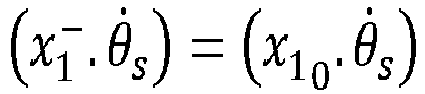
  • S s 0 ⁇ x 1 ⁇ . ⁇ ⁇ O ⁇ x 1 0 .
  • a process noise ( Q 1 ) may be added to the calibration parameters covariance as it may be slightly changing over time for mainly temperature/pressure changes. Such added process noise may lead to force retuning of the parameters when significantly long time passed without adaption.
  • ⁇ S x ⁇ 1 ⁇ .
  • the GNSS measurement state Z 1 is presented with mean ⁇ 1 and covariance R 1 .
  • the covariance matrix of the GNSS measurements can be set to a diagonal matrix, with each of the diagonal elements presents the variance of one of the state elements assuming no correlation between them as follows.
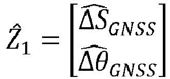
  • Z 1 ⁇ S GNSS ⁇ GNSS
  • Z ⁇ 1 ⁇ S ⁇ GNSS ⁇ ⁇ GNSS
  • R 1 ⁇ ⁇ S GNSS 2 0 0 ⁇ ⁇ GNSS 2
  • the standard deviation provided in the GNSS data for both the GNSS estimated speed and heading shall be used.
  • the signals sigma_speed and sigma_heading provided by GNSS can be used to present the standard deviation in the GNSS speed ( ⁇ v GNSS ) and the standard deviation in the GNSS heading ( ⁇ ⁇ GNSS ) , respectively at every GNSS location point.
  • the computing of the variance of the driven distance ( ⁇ ⁇ S GNSS ) 2 and orientation change ( ⁇ ⁇ ⁇ GNSS ) 2 along GNSS track can be formulated as follows.
  • ⁇ S GNSS is the driven distance along GNSS track
  • v i GNSS is the speed provided by GNSS data at every GNSS location point with index i
  • ⁇ t i GNSS is the time span of the GNSS provided data at index i till the data in the next step is provided.
  • the orientation change is the difference in the heading at the final and initial points along the track with length of n points.
  • ( v s ) denote a scaling factor of the vehicle's input speed from one cycle to another (for example from a previous cycle to a current cycle).
  • the scaling factor may be computed as the ratio between the speed in the current cycle ( v n ) and the speed in the previous cycle ( v 0 ).
  • may be greater than zero. This yields:
  • the method may overwrite the speed in the state of the Fusion block 2 with the input speed ( v n ) projected on the vehicle's cartesian ( x , y ) coordinates.
  • x 2 0 x x
  • v y ⁇ x 2 0 .
  • v x v s ⁇ sin rot ⁇ x 2 ⁇ . x ⁇ x 2 0 .
  • v y ⁇ x 1 n .
  • v y x 1 n .
  • v y ⁇ v s ⁇ sin rot ⁇ x 2 ⁇ . v y ⁇ x ⁇ 2 0 .
  • v y v s ⁇ cos rot
  • the matrix F 2 x 2 has a first column with components: 1 1 0 ′ 0
  • the matrix F 2 x 2 has a second column with components: 0 1 0 ′ 0
  • the matrix F 2 x 2 has a third column with components: x ⁇ 1 n .
  • the matrix F 2 x 2 has a fourth column with components: ⁇ x ⁇ 1 n .
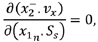
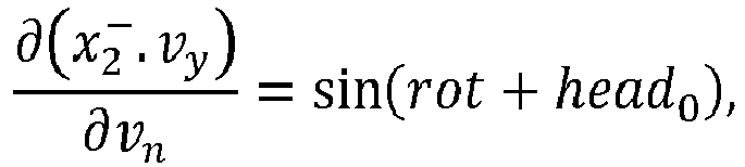
  • the method may consider the following equations: ⁇ x 2 ⁇ . x ⁇ x 1 n .
  • S s v s ⁇ x ⁇ 2 0 . v x ⁇ cos rot ⁇ x ⁇ 2 0 . v y ⁇ sin rot ⁇ ⁇ t , ⁇ x 2 ⁇ . y ⁇ x 1 n .
  • S s v s ⁇ x ⁇ 2 0 . v x ⁇ sin rot ⁇ x ⁇ 2 0 . v y ⁇ cos rot ⁇ ⁇ t , ⁇ x 2 ⁇ . v x ⁇ x 1 n .
  • ⁇ ⁇ o v s ⁇ x ⁇ 1 n .
  • ⁇ ⁇ o v s ⁇ ⁇ x ⁇ 2 0 . v x ⁇ sin rot ⁇ x ⁇ 2 0 . v y ⁇ cos rot ⁇ ⁇ t , ⁇ x 2 ⁇ . v x ⁇ x 1 n .
  • the method may consider a matrix F 2 x 1 with a first column having components v s ⁇ x ⁇ 2 0 . v x ⁇ cos rot ⁇ x ⁇ 2 0 . v y ⁇ sin rot ⁇ ⁇ t v s ⁇ x ⁇ 2 0 . v x ⁇ sin rot + x ⁇ 2 0 . v y ⁇ cos rot ⁇ ⁇ t 0 0
  • the matrix F 2 x 1 also has a second column having components v s ⁇ x ⁇ 1 n .
  • v y sin rot ⁇ ⁇ ⁇ n ⁇ ⁇ t 2 v s ⁇ ⁇ x ⁇ 2 0 .
  • the matrix F 2 x 1 also has a third column having components v s ⁇ x ⁇ 1 n .
  • the current heading of the vehicle's motion is presented by the speed components in the state as follows.
  • S s ⁇ cos rot + head 0 ⁇ ⁇ t , ⁇ x 2 ⁇ . y ⁇ v n x ⁇ 1 n .
  • v y ⁇ v n sin rot + head 0 , ⁇ x 2 ⁇ .
  • x ⁇ ⁇ ⁇ n ⁇ v n ⁇ x ⁇ 1 n .
  • S s ⁇ x ⁇ 1 n . ⁇ ⁇ s ⁇ sin rot + head 0 ⁇ ⁇ t 2 , ⁇ x 2 ⁇ . y ⁇ ⁇ ⁇ n v n ⁇ x ⁇ 1 n .
  • v x ⁇ ⁇ n ⁇ v n ⁇ x ⁇ 1 n .
  • S s ⁇ x ⁇ 1 n .
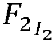
  • I 2 is a matrix having a left column with components : x ⁇ 1 n . S s ⁇ cos x ⁇ 1 n . ⁇ ⁇ s ⁇ ⁇ ⁇ n + x ⁇ 1 n .
  • x x ⁇ 2 ⁇ . x x ⁇ 2 m .
  • y x ⁇ 2 ⁇ . y x ⁇ 2 m .
  • v x x ⁇ 1 n . S s ⁇ x ⁇ 2 ⁇ . v x ⁇ 2 m .
  • v y x ⁇ 1 n .
  • S s ⁇ x ⁇ 2 ⁇ . v y H 2 x 2 ⁇ x 2 m ⁇ x 2 ⁇
  • P 2 n P 2 ⁇ ⁇ K 2 H 2 x 2 P 2 ⁇ .
  • the GNSS measurement state Z 2 is presented with mean ⁇ 2 and covariance R 2 .
  • the covariance matrix of the GNSS measurements can be set to a diagonal matrix, with each of the diagonal elements presents the variance of one of the state elements assuming no cross correlation between them as follows.
  • the standard deviation provided in the GNSS data for both the GNSS estimated speed and heading shall be used.
  • the signals sigma_speed and sigma_heading provided by GNSS can be used to present the standard deviation in the GNSS speed ( ⁇ v GNSS ) and the standard deviation in the GNSS heading ( ⁇ ⁇ GNSS ) , respectively at every GNSS location point.
  • the Horizontal Estimated Position Error ( HEPE ) and Horizontal Dilution Of Precision ( HDOP ) signals shall be used to estimate the position errors, especially the second one according to reference M.
  • ⁇ GNSS presents the heading obtained from GNSS at the previous GNSS cycle
  • ⁇ t GNSS presents the cycle time of the input GNSS data
  • ⁇ ⁇ presents the variance in the input yaw rate, which is used as well in Q
  • ⁇ ⁇ t GNSS presents the variance in the cycle time of the GNSS. Both can be predefined according to the available GNSS data.
  • ⁇ v x GNSS 2 sin 2 ⁇ GNSS + ⁇ ⁇ avg ⁇ ⁇ t GNSS ⁇ v GNSS 2 + v GNSS 2 cos 2 ⁇ GNSS + ⁇ ⁇ avg ⁇ ⁇ t GNSS ⁇ ⁇ GNSS 2 + v GNSS 2 cos 2 ⁇ GNSS + ⁇ ⁇ avg ⁇ ⁇ t GNSS ⁇ t GNSS 2 ⁇ ⁇ ⁇ 2 + v GNSS 2 cos 2 ⁇ GNSS + ⁇ ⁇ avg ⁇ ⁇ t GNSS ⁇ t GNSS 2 ⁇ ⁇ ⁇ 2 + v GNSS 2 cos 2 ⁇ GNSS + ⁇ ⁇ avg ⁇ ⁇ t GNSS ⁇ ⁇ 2 ⁇
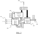
  • FIG. 2 shows a diagram illustration of implementations of the fusion blocks 1 and 2 by the method.
  • the method also obtains, while the GNSS signal is available, GNSS data 220.
  • the GNSS data 220 comprises a driven distance for the vehicle denoted by ⁇ S and orientation change denoted by ⁇ ⁇ for the vehicle.
  • the GNSS data 220 further includes a location and heading of the vehicle denoted by [ x, y, v x , v y ].
  • the method calibrates parameters of the odometer 230.
  • the parameters of the odometer 230 include speed scaling, the vehicle yaw rate scaling, and the vehicle yaw rate offset denoted as [ S s , ⁇ s , ⁇ o ],
  • the calibration is based on a data fusion that uses a Kalman filter 240 (denoted as Fusion block 1) that determines a predicted distance variation and a predicted orientation variation of the vehicle based on the current calibration parameters of the odometer 230 and on the motion data 210.
  • the Kalman filter 240 compares the predicted distance variation and predicted orientation variation to the distance variation and the orientation variation of the GNSS data 220.
  • the method determines a localization 260 of the vehicle by performing a data fusion that is based on a Kalman filter 250 (denoted as Fusion block 2) that predicts the vehicle localization based on a fusion of the location and heading [ x, y, v x , v y ] of the GNSS data 220 and a location and heading predicted, from the odometer 230, according to the calibrated odometer parameters.
  • Fusion block 2 a Kalman filter 250 that predicts the vehicle localization based on a fusion of the location and heading [ x, y, v x , v y ] of the GNSS data 220 and a location and heading predicted, from the odometer 230, according to the calibrated odometer parameters.
  • the method determines a localization 260 of the vehicle based on a location and heading predicted according to the calibrated odometer parameters.
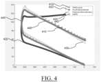
  • FIG.s 3 and 4 illustrate the performance of the method for Dead Reckoning localization. The performance is evaluated by comparing the computed vehicle location from the prediction odometer equations using the calibrated Odometer parameters against the vehicle location from a reference Differential GPS (DGPS).
  • DGPS Differential GPS
  • the tracks input to the Fusion block 1 are selected by filtering the straight motion parts where the displacement is the track length and orientation change is almost zero.
  • FIG. 3 shows the vehicle's straight motion so as to illustrate the calibration of the speed scale parameter, represented with GNSS points 310 stemming from the GNSS data, the pure prediction model 320, the prediction after calibration of the odometer 330 and the reference DGPS 340.
  • the x-axis in FIG. 3 corresponds to the x-coordinates in cartesian coordinates of the projection of the vehicle to the ground. Accordingly, the y-axis corresponds to the y-coordinates in cartesian coordinates.
  • the straight motion trace plotted in FIG. 3 has at least one straight motion track, where the Fusion block 1 calibrates the speed scale. Moreover, the not-counter steering tracks with yaw rate having same sign connecting two straight motions are selected for the comparison of the predicted distance variation and predicted orientation variation to the distance variation and the orientation variation of the GNSS data. For such tracks, the displacement is the track length, and the orientation change is the difference in the angles of the two straight lines at the start and end of the track.
  • FIG. 4 shows the vehicle's U-shape motion so as to illustrate the calibration of both the yaw rate scale and offset parameters, represented with GNSS points 410 stemming from the GNSS data, the pure prediction model 420, the prediction after calibration of the odometer 430 and the reference DGPS 440.
  • the x-axis in FIG. 4 corresponds to the x-coordinates in cartesian coordinates of the projection of the vehicle to the global earth horizontal east direction.
  • the y-axis corresponds to the y-coordinates in cartesian coordinates of the projection of the vehicle to the global earth vertical north direction.
  • the circular path 440 connecting the two straight segments is selected as a track for fusion to calibrate the yaw rate scaling and offset where the orientation difference is approximately 180°.
  • the straight motion track is filtered by fetching GNSS location points stored in history over specified time window. Then, line fitting is done for the GNSS points that achieves the least sum of square of the perpendicular distances from the points to the fitting line. If the mean of the absolute values of the perpendicular distances is less than specific threshold, then the GNSS points are categorized as straight motion track to be selected as input to Fusion block 1.
  • FIG.s 3 and 4 show how the predicted location of the vehicle based on the calibrated parameters in green is enhanced compared to the predicted location of the vehicle without parameters calibration in blue. Both are evaluated against the reference DGPS location in solid red, while the GNSS locations received at lower rate are the red points. It is clear from the figures the enhancement in localization after applying the proposed design for dynamic calibration of the parameters of the odometer.
  • P 2 n E x 2 n ⁇ x ⁇ 2 n x 2 n ⁇ x ⁇ 2 n T
  • P 2 n E x 2 ⁇ + K 2 Z 2 ⁇ h 2 x 2 ⁇ x 1 n ⁇ x ⁇ 2 ⁇ ⁇ K 2 Z ⁇ 2 ⁇ 2 h 2 x ⁇ 2 ⁇ 2 ⁇ 2 ⁇ 2
  • ⁇ Ax ⁇ x A ⁇ x T
  • a ⁇ x A T ⁇ x T
  • a x ⁇ x 2 x T
  • K 2 P 2 ⁇ H 2 x 2 T R + H 2 x 2 P 2 ⁇ H 2 x 2 T + H 2 x 1 P 1 n H 2 x 1 T
  • K 2 P 2 ⁇ H 2 x 2 T H 2 x 2 P 2 ⁇ H 2 x 2 T + H
  • K 2 H 2 x 2 P 2 ⁇ P 2 ⁇ H 2 x 2 T H 2 x 2 P 2 ⁇ H 2 x 2 T + H 2 x 1 P 1 n H 2 x 1 T + R ⁇ 1 H 2 x 2 P 2 ⁇ P 2 ⁇ H 2 x 2 T

Landscapes

  • Engineering & Computer Science (AREA)
  • Radar, Positioning & Navigation (AREA)
  • Remote Sensing (AREA)
  • Physics & Mathematics (AREA)
  • General Physics & Mathematics (AREA)
  • Computer Networks & Wireless Communication (AREA)
  • Automation & Control Theory (AREA)
  • Manufacturing & Machinery (AREA)
  • Navigation (AREA)

Abstract

The disclosure notably relates to a computer-implemented method for localization of a moving vehicle based on GNSS data and vehicle sensor data. The method comprises, in real-time, obtaining vehicle motion data stemming from at least one vehicle sensor. The method also comprises obtaining, while the GNSS signal is available, GNSS data of a positioning of the vehicle. The GNSS data includes a distance variation and an orientation variation. The method also comprises calibrating parameters of an odometer of the vehicle. The calibration is based on a data fusion that uses a Kalman filter. The Kalman filter determines a predicted distance variation and a predicted orientation variation of the vehicle based on a current calibration of the odometer parameters and on the motion data. The Kalman filter also compares the predicted distance variation and predicted orientation variation to the distance variation and the orientation variation of the GNSS data.

Description

    TECHNICAL FIELD
  • The disclosure relates to the field of computer programs and systems, and more specifically to a method, system and program for localization of a moving vehicle.
  • BACKGROUND
  • A number of systems and programs are offered on the market for tracking the localization of a vehicle.
  • Within this context, there is still a need for an improved method for localization of a moving vehicle.
  • SUMMARY
  • It is therefore provided a computer-implemented method for localization of a moving vehicle based on GNSS data and vehicle sensor data. The method comprises, in real-time, obtaining vehicle motion data. The vehicle motion data stems from at least one vehicle sensor. The method also comprises, in real-time, obtaining, while the GNSS signal is available, GNSS data of a positioning of the vehicle. The GNSS data includes a distance variation and an orientation variation. The method also comprises, in real-time, calibrating parameters of an odometer of the vehicle. The calibration is based on a data fusion that uses a Kalman filter. The Kalman filter determines a predicted distance variation and a predicted orientation variation of the vehicle based on a current calibration of the odometer parameters and on the motion data. The Kalman filter also compares the predicted distance variation and predicted orientation variation to the distance variation and the orientation variation of the GNSS data.
  • The method may comprise one or more of the following:
    • the odometer predicts cyclically in time a new location of the vehicle and a new heading of the vehicle based on a location and heading predicted at the previous cycle and on the motion data;
    • the motion data includes the vehicle speed in the current cycle, the vehicle speed in the previous cycle, and the vehicle yaw rate in the current cycle;
    • the parameters of the odometer include a vehicle speed scaling, a vehicle yaw rate scaling, and a vehicle yaw rate offset;
    • calibrating parameters includes correcting one or any combination of the vehicle speed scaling, the vehicle yaw rate scaling, and the vehicle yaw rate offset;
    • the motion data stems from a wheel sensor, an Inertial Measurement Unit (IMU), and a steering system sensor;
    • the GNSS data further includes a location and heading of the vehicle, and the method further comprises, in real-time:
      • when the GNSS signal is available, determining a localization of the vehicle by performing a data fusion that is based on a Kalman filter that predicts the vehicle localization based on a fusion of the location and heading of the GNSS data and a location and heading predicted according to the calibrated odometer parameters;
      • when the GNSS signal is lost, determining a localization of the vehicle based on a location and heading predicted according to the calibrated odometer parameters;
    • the GNSS data stems from a GNSS device that comprises only one antenna; and/or
    • the vehicle is a motorbike, a car, a bus or a truck.
  • It is further provided a computer program comprising instructions which, when executed by a computer system, cause the system to perform the method.
  • It is further provided a computer readable storage medium having recorded thereon the computer program.
  • It is further provided a system comprising a processor coupled to a memory, the memory having recorded thereon the computer program.
  • The system may comprise one or more of the following:
    • the system is coupled with or further comprises the GNSS device, the odometer, and the at least one sensor; and/or
    • the at least one sensor includes a wheel sensor, an Inertial Measurement Unit (IMU), and a steering system sensor;
  • It is further provided a vehicle equipped with the system.
  • BRIEF DESCRIPTION OF THE DRAWINGS
  • Non-limiting examples will now be described in reference to the accompanying drawings, where:
    • FIG. 1 shows an example of the system; and
    • FIG.s 2 to 4 illustrate the method.
    DETAILED DESCRIPTION
  • It is proposed a computer-implemented method for localization of a moving vehicle based on Global Navigation Satellite System (also called GNSS herein below) data and vehicle sensor data. The method comprises, in real-time, obtaining vehicle motion data. The vehicle motion data stems from at least one vehicle sensor. The method also comprises, in real-time, obtaining, while the GNSS signal is available, GNSS data of a positioning of the vehicle. The GNSS data includes a distance variation and an orientation variation. The method also comprises, in real-time, calibrating parameters of an odometer of the vehicle. The calibration is based on a data fusion that uses a Kalman filter. The Kalman filter determines a predicted distance variation and a predicted orientation variation of the vehicle based on a current calibration of the odometer parameters and on the motion data. The Kalman filter also compares the predicted distance variation and predicted orientation variation to the distance variation and the orientation variation of the GNSS data.
  • Such a method improves the localization of the moving vehicle.
  • Notably, the method achieves an improved accuracy for localizing the moving vehicle regardless of where the vehicle may be spatially localized, for example, regardless of whether the vehicle is localized inside a tunnel or in an open field. This is because the localization of the vehicle is determined from two types of data: the vehicle motion data and the GNSS data while the GNSS signal is available. On one hand, vehicle motion data consists on local data which is acquired from the at least one vehicle sensor (for example comprising a wheel sensor, an Inertial Measurement Unit (IMU), and a steering system sensor) and thus provides data about the vehicle motion. On the other hand, the GNSS data provides an accurate data of positioning of the vehicle (including GNSS motion data such as the distance variation and the orientation variation) while the GNSS signal is available, for example, in an open field covered by GPS coverture (which is the case during the majority of the vehicle's trip, except on short periods where the vehicle goes through a tunnel or the like). However, the vehicle motion data on its own is sensible to sensor-related errors. For example, the speed obtained from a sensor such as a wheel encoder may be based on a default tire size (wheel circumference), which could vary due to change of tire pressure/temperature or exchanging the tires with others with different circumference like the summer/winter exchange. Such change in the tire size may introduce scaling factor error in the measured speed. Moreover, a sensor such as an IMU provides angular speeds and acceleration for yaw, pitch, and roll based on builtin gyroscope. The readings of such electro-mechanical sensor may be highly affected by significant temperature/pressure changes, and a slight shift in the mounting of the sensor shall introduce bias error to it. Finally, a sensor such as a steering system sensor is based on feeding back the place of the slider on the steering rack to indicate the steering measurement, which may present offset errors due to its mechanical sliding resolution. Hence, the Odometer sensors scaling and offset errors may be dynamically changing, and the present method may estimate them continuously in order to locate the vehicle accurately. However, as the method also relies also on the GNSS data, the method re-calibrates the odometer using the GNSS data, which is known to be particularly reliable, so as to compensate for such errors.
  • Indeed, thanks to the method achieving a continuous calibration of the parameters of the odometer of the vehicle, the method further improves the robustness for localizing the vehicle based on both the vehicle motion data and the GNSS data. As outlined above, the odometer (providing information on the motion of the vehicle) may be subject to changes in pressure and/or temperature which may introduce error factors in the vehicle motion data stemming from the at least one sensor. However, thanks to the use of the Kalman filter, the method determines a predicted distance variation and a predicted orientation variation based on a data fusion of the GNSS and sensor data so that the method corrects parameters of the odometer based on the comparison of the predicted (i.e. using the sensor motion data) distance variation and predicted (i.e. using the sensor motion data) orientation variation to the distance variation and the orientation variation of the GNSS data. Due to the method performing the signals capturing in real time, the calibration is also done relatively continuously (e.g., continuously while the GNSS signal is available, e.g. at regular and short time intervals/steps) and thus the odometer is persistently calibrated as the comparison is done every time there is a track (that is, a distance traveled by the vehicle) that can be extracted from both the odometer and GNSS data, for example where there is suitable coverage from a GNSS system such as satellites. In other words, upon losing the GNSS data, the calibrated odometer, which is conform to the last available GNSS data, makes on its own accurate prediction using the calibrated parameters during the absence of the GNSS data. In yet other words, as long as the GNSS data is available, which again corresponds the majority of the vehicle's trip, the odometer is continuously/in real-time calibrated and the vehicle localization can be determined based on the calibrated odometer and on the GNSS and sensor data. When the GNSS data is lost, for example in a tunnel, which often correspond to a relatively short period of time comparted to the duration of the vehicle's trip, localization can be made on the sole prediction performed by the odometer based on the lastly calibrated parameters and based on the sensor motion data.
  • The method is computer-implemented. This means that steps (or substantially all the steps) of the method are executed by at least one computer, or any system alike. Thus, steps of the method are performed by the computer, possibly fully automatically, or, semi-automatically. In examples, the triggering of at least some of the steps of the method may be performed through user-computer interaction. The level of user-computer interaction required may depend on the level of automatism foreseen and put in balance with the need to implement user's wishes. In examples, this level may be user-defined and/or pre-defined.
  • A typical example of computer-implementation of a method is to perform the method with a system adapted for this purpose. The system may comprise a processor coupled to a memory and a graphical user interface (GUI), the memory having recorded thereon a computer program comprising instructions for performing the method. The memory may also store a database. The memory is any hardware adapted for such storage, possibly comprising several physical distinct parts (e.g. one for the program, and possibly one for the database). The system may be coupled or further comprise the GNSS device, the odometer, and the at least one sensor. The at least one sensor may include a wheel sensor, an Inertial Measurement Unit (IMU), and a steering system sensor.
  • FIG. 1 shows an example of the system, wherein the system is a computer system 100 configured to be mounted on a vehicle.
  • The computer 100 of the example comprises a processor or processing unit such as a central processing unit (CPU) 1010 connected to an internal communication BUS 1000. A random access memory (RAM) may be optionally connected to the BUS (not shown). A memory controller 1020 manages accesses to a mass memory device, such as hard drive or other form of non-volatile memory such as EPROM, EEPROM, and flash memory devices. Any of the foregoing may be supplemented by, or incorporated in, specially designed ASICs (application-specific integrated circuits). The computer may optionally also include a display, e.g., a touch screen (not shown). The display may be configured for displaying the localization of the vehicle. The computer 100 may be coupled with a GNSS 1080 through a port or interface 1090 and with a wheel sensor 1050 like a wheel encoder, an IMU 1040 and a steering system sensor 1030 through a port or interface 1060. The computer 100 may comprise an output port 1070 for sending calibration parameters to the odometer 1110. The computer 100 may also comprise an output port 1100 for outputting the data forming the vehicle's predicted localization. The odometer 1110 may be coupled with the computer 100 as shown in the figure to send its predictions to the computer. The data may comprise the localization and the heading of the vehicle and any other localization data discussed herein. The display may also be configured for displaying the localization of the vehicle.
  • The computer program may comprise instructions executable by a computer, the instructions comprising means for causing the above system to perform the method. The program may be recordable on any data storage medium, including the memory of the system. The program may for example be implemented in digital electronic circuitry, or in computer hardware, firmware, software, or in combinations of them. The program may be implemented as an apparatus, for example a product tangibly embodied in a machine-readable storage device for execution by a programmable processor. Method steps may be performed by a programmable processor executing a program of instructions to perform functions of the method by operating on input data and generating output. The processor may thus be programmable and coupled to receive data and instructions from, and to transmit data and instructions to, a data storage system, at least one input device, and at least one output device. The application program may be implemented in a high-level procedural or object-oriented programming language, or in assembly or machine language if desired. In any case, the language may be a compiled or interpreted language. The program may be a full installation program or an update program. Application of the program on the system results in any case in instructions for performing the method. The computer program may alternatively be stored and executed on a server of a cloud computing environment, the server being in communication across a network with one or more clients. In such a case a processing unit executes the instructions comprised by the program, thereby causing the method to be performed on the cloud computing environment.
  • It is further provided a vehicle equipped with the system. The vehicle may be a motorbike, a car, a bus or a truck.
  • The method is for determining the localization of the moving vehicle, that is, the spatial location of the vehicle as it follows a generally continuous movement (this does however not exclude vehicle stops, for example at red lights). The localization may be expressed in terms of the 3D cartesian coordinates (x,y,z) with z denoting (by convention) an altitude of the vehicle with respect to the x-y plane or 2D cartesian coordinates (x,y), by considering the projection of the vehicle to the ground in the x-y plane. The method may output the localization of the vehicle. For example, the method may output the location of the vehicle in 3D or 2D cartesian coordinates. The method may also output the speed of the vehicle, the heading and/or the yaw rate.
  • Steps of the method are performed in real-time. In other words, steps of the method may be performed each in a relatively short time (for example in the order of milliseconds) so that the duration of the steps is low enough to so as to appear continuous (within a discrete approximation).
  • The vehicle motion data is obtained (as it stems from the at least one vehicle sensor) in real time, that is, as a sequence of discrete values being separated by a short time-difference. The GNSS data is also obtained in real time while the GNSS signal is available. The method may obtain the vehicle motion data and/or the GNSS data as a sequence of values. The sequence of values may be time-ordered, i.e., the vehicle motion data and the GNSS data may be time-ordered sequences, where respective values are ordered according to the time by which the value was obtained. Each value in a respective time-ordered sequence may be associated with a time-stamp. The time-stamp may be a piece of data comprising a value of time, e.g., a time (having for example date and hour or alternatively indicated by an index) in which the vehicle motion data is acquired by the at least one vehicle sensor (in the case of the vehicle motion data) or a time in which the GNSS data is acquired while the GNSS signal is available. In examples, two values of the sequence of values may be separated by a time difference, for example an uniform time-difference between each other (for example, two consecutive values) or alternatively, by a non-uniform time-difference between two values.
  • The vehicle motion data stems from at least one vehicle sensor. In other words, values obtained from vehicle motion data are the result of the measurement by the sensor corresponding to the vehicle's motion. By "motion data" it is meant any time-ordered sequence of values indicative of the vehicle's motion, for example indicating a position, speed, yaw and/or steering. The motion data may stem from a wheel sensor, an Inertial Measurement Unit (IMU), and a steering system sensor. In other words, the vehicle motion data may stem from the wheel sensor, the Inertial Measurement Unit (IMU), and the steering system sensor.
  • The method obtains in real-time, while the GNSS signal is available, GNSS data of a positioning of the vehicle. The GNSS data includes a distance variation and an orientation variation. The GNSS data may be a time-ordered sequence of values, each value including the distance variation and a orientation variation at each respective time. The "distance variation" may mean any variation of the distance travelled by the vehicle in a predetermined time-step according to the measurements of the GNSS data. The "orientation variation" may mean any variation of the orientation of the vehicle in a predetermined time-step according to the GNSS data. In other words, the GNSS data of the altitude of the vehicle is provided from the Global Navigation Satellite System while the GNSS signal is available, for example when the vehicle is in an open area with GNSS coverage. The Global Navigation Satellite System may be for example the GPS system, GLONASS or GALILEO navigation system.
  • The method calibrates in real-time parameters of the odometer. By "calibration" it is to be understood that the method modifies the parameters of the odometer so that the odometer makes vehicle localization predictions that are in line with the GNSS data. The parameters of the odometer may include a vehicle speed scaling, a vehicle yaw rate scaling, and a vehicle yaw rate offset. The method may calibrate only one of the vehicle scaling, the vehicle yaw rate scaling or the vehicle yaw rate offset. Alternatively, the method may calibrate more than one (for example all) of the parameters.
  • The calibration is based on a data fusion that uses a Kalman filter. By "data fusion" it is meant that the vehicle motion data is used concomitantly with the GNSS data (for example by comparing the vehicle motion data with the GNSS data, while the GNSS signal is available) for calibrating parameters of the odometer. The Kalman filter (also denoted herein below as a "Fusion block 1") determines a predicted distance variation and a predicted orientation variation of the vehicle based on a current calibration of the odometer parameters and on the motion data. This correspond to the prediction step of the Kalman filter, as known per se from Kalman filters. The Kalman filter also compares the predicted distance variation and predicted orientation variation to the distance variation and the orientation variation of the GNSS data. This correspond to the correction step of the Kalman filter, as known per se from Kalman filters.
  • The GNSS data may stem from a GNSS device that comprises only one antenna. The only one antenna may be configured to receive the signal from the GNSS system, such as the GPS system. As the method comprises only one antenna, the system is simple and cheap as it relies on less resources for obtaining the GNSS data. In addition, the localization is made entirely online, so that the use of localization sensors or lasers may be avoided (which may add further errors and cost).
  • The odometer may predict cyclically in time a new location of the vehicle and a new heading of the vehicle based on a location and heading predicted at the previous cycle and on the motion data. In other words, the odometer may perform the prediction periodically (e.g., at regular and short time steps) based on a location and heading predicted at a timing prior to the prediction (e.g. at the previous time step). "Current cycle" may refer to the current time step, and "previous cycle" may refer to the preceding/previous time step. This ensures that the filter Kalman provides a sequential and cyclical prediction of the location as it receives the motion data and the GNSS data.
  • The odometer may predict cyclically in time the new location of the vehicle and the new heading of the vehicle as variables [x, y, vx, vy ] based on the location predicted at the previous cycle and heading of the previous cycle and on motion data I = {vn, v 0 , θ̇ n}. The variables x, y denote the location of the vehicle in an x-y plane. The variables vx, vy denote the speed components of the vehicle. The vehicle's heading angle is denoted by tan 1 v y v x
    Figure imgb0001
    .
  • The motion data may include the vehicle speed in the current cycle, the vehicle speed in the previous cycle (at a timing preceding the current cycle), and the vehicle yaw rate in the current cycle. The motion data may be captured as the formula I = {vn, v 0 , θ̇n } (e.g. implemented in the computer using this formula), including the variables vn, v 0 , θ̇n, where vn denotes the vehicle speed in the current cycle, v0 denotes the vehicle speed in the previous cycle, and θ̇ n denotes the vehicle yaw rate in the current cycle.
  • Calibrating parameters of the odometer may include correcting one or any combination of the vehicle speed scaling, the vehicle yaw rate scaling, and the vehicle yaw rate offset. The calibration of the parameters of the odometer allows to compensate scaling and offset errors in the vehicle motion data, thereby improving the real-time estimation of the positioning of the vehicle.
  • The parameters of the odometer may be the vehicle speed scaling, the vehicle yaw rate scaling, and the vehicle yaw rate offset, for example respectively denoted as [Ss, θ̇s, θ̇o ]. The parameters of the odometer may be calibrated by comparing a distance variation ΔS (also referred to as "driven distance") and an orientation variation/change Δθ (computed by the Odometer for a specific vehicle's track) with a corresponding distance variation ΔS and orientation variation Δθ included in the GNSS data.
  • The Kalman filter that determines the predicted distance variation and the predicted orientation variation of the vehicle may be denoted mathematically by a prediction function f 1() that receives the initial state of the parameters output from a previous cycle ( 10 ) and the current vehicle motion data (I 1) (obtained at a current cycle) to generate a priori predicted state of the parameters ( x ^ 1
    Figure imgb0002
    ). The priori predicted state is fed to a function h 1(). The function h 1() converts the priori predicted state to the measurement space where the predicted measurement (x̂1m ) is obtained. The Kalman filter computes the fused posteriori state (x̂1n ) based on the Kalman innovation, which is the difference between the measurement from GNSS data and the predicted measurement from motion signals.
  • The vehicle motion data (I 1) may be presented with the integrals of the speed signals and yaw rate signals along the track beside the elapsed time (ΔT) along the track, so as to take into account that the Kalman filters determines the predicted distance variation and the predicted orientation variation of the vehicle on a track between the current cycle and the previous cycle. The method may use such integrals to output a resulting driven distance (ΔSin ) and orientation change (Δθin ) of the track from the vehicle motion data, which is presented with (n) samples of input signals of vehicle speed (vi ) and yaw rate (θ̇i ) coming at time intervals (Δti ). ΔS in = i = 1 n v i × Δt i
    Figure imgb0003
    Δθ in = i = 1 n θ ˙ i × Δt i
    Figure imgb0004
    ΔT = i = 1 n Δt i
    Figure imgb0005
    I 1 = ΔS in Δθ in ΔT
    Figure imgb0006
    x 1 = f 1 x 1 0 I 1
    Figure imgb0007
    x ^ 1 = f 1 x ^ 1 0 I 1
    Figure imgb0008
    S s θ ˙ s θ ˙ O x ^ 1 = f 1 S s θ ˙ s θ ˙ O , I 1 x ^ 1 0
    Figure imgb0009
    x ^ 1 m = ΔS m Δθ m
    Figure imgb0010
    x ^ 1 m = h 1 x ^ 1 I 1
    Figure imgb0011
    Z 1 = ΔS GNSS Δθ GNSS
    Figure imgb0012
    x ^ 1 n = x ^ 1 + K 1 Z 1 x ^ 1 m
    Figure imgb0013
  • The GNSS data may further include a location and heading of the vehicle. The method may further comprise, in real-time, when the GNSS signal is available, determining a localization of the vehicle by performing a data fusion that is based on a Kalman filter (also denoted herein below as "Fusion block 2") that predicts the vehicle localization based on fusion of the location and heading of the GNSS data and a location and heading predicted according to the calibrated odometer parameters. it is meant that the method uses the usual Kalman filter methods for performing the prediction and calibration. The method may calibrate the parameters of the odometer based on the predicted vehicle localization. In examples, the method may set the parameters of the odometer after determining the localization of the vehicle. This ensures that the calibration is performed dynamically.
  • The method may obtain from the odometer the vehicle's position and heading based on the result of the comparison (that is, the latest modified calibration parameters), which may be added to the vehicle position and heading that are fused with the ones obtained from GNSS in the Fusion block 2 to generate the vehicle's location.
  • The method may further comprise, in real-time, when the GNSS signal is lost, determining a localization of the vehicle based on a location and heading predicted according to the calibrated odometer parameters. In other words, upon losing GNSS data (for instance whenever the vehicle is on an area not covered by GNSS signal such as a tunnel or interior area), the method determines the localization of the vehicle using only the prediction of the vehicle's heading and position (which then form the localization data) by the odometer according to its calibrated parameters (that is, according to the parameters lastly calibrated according of the lastly available GNSS data). In yet other words, the odometer thus relies on such calibration while the GNSS data is lost, and the localization determination is solely based on the odometer's processing of the motion data according to this calibration. When the GNSS signal is recovered, the method may perform the calibration again as describe above and thus re-adjusts the odometer with the available GNSS data.
  • This further improves the accuracy of the calibration of the odometer, as the method accurately determines the location of the vehicle, including the steering. This is because the method determines the location and heading according to the calibrated parameters of the odometer, and thus, according to odometer parameters that are in line with the lastly available GNSS data, and that are thereby reliable. Moreover, as the calibration is performed dynamically, the method feeds back the odometer to recalibrate the odometer, thereby reducing bias errors that may be present in electro-mechanical sensors.
  • Examples of the Kalman Filter that predicts the vehicle localization are now discussed. Let [Ss, θ̇s, θ̇o ] (which denote the parameters of the odometer) denote state of the Kalman filter that determines a predicted distance variation and a predicted orientation variation of the vehicle (that is, the Fusion block 1). Let [x, y, vx, vy ] denote the state of the Kalman filter that predicts the localization of the vehicle (That is, the Fusion block 2), the state representing [x, y, vx, vy ]the vehicle's position and orientation presented with the vehicle velocity components in x and y directions.
  • The Kalman's filter corresponding to Fusion block 2 is denoted by the equations: I 2 = v n v 0 θ ˙ n ,
    Figure imgb0014
    x 2 = f 2 x 2 0 x 1 n I 2 ,
    Figure imgb0015
    x ^ 2 = f 2 x ^ 2 0 x ^ 1 n I 2 ,
    Figure imgb0016
    x y v x v y x ^ 2 = f 2 x y v x v y x ^ 2 0 S s θ ˙ s θ ˙ O x ^ 1 n I 2 ,
    Figure imgb0017
    Z 2 = x GNSS y GNSS v x GNSS v y GNSS ,
    Figure imgb0018
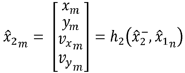
    x ^ 2 m = h 2 x ^ 2 x ^ 1 n ,
    Figure imgb0019
    x ^ 2 n = x ^ 2 + K 2 Z ^ 2 x ^ 2 m .
    Figure imgb0020
  • The method may calibrate the parameters of the odometer dynamically, based on the Fusion block 1. The method may perform a fusion of the prediction of the vehicle localization and the adaptation may be expressed mathematically by a mean equation x ^ 1 x ^ 1 n
    Figure imgb0021
    and a covariance equation P 1 P 1 n
    Figure imgb0022
    expressed as follows: x 1 = f 1 x 1 0 I 1
    Figure imgb0023
    x ^ 1 = f 1 x ^ 1 0 I 1
    Figure imgb0024
    I 1 = ΔS in Δθ in ΔT
    Figure imgb0025
    x 1 . S s = x 1 0 . S s
    Figure imgb0026
    x 1 . θ ˙ s = x 1 0 . θ ˙ s
    Figure imgb0027
    x 1 . θ ˙ O = x 1 0 . θ ˙ O
    Figure imgb0028
    F 1 x = x 1 x 1 0 | x 1 0 = x ^ 1 0 = f 1 x 1 0 I 1 x 1 0 | x 1 0 = x ^ 1 0 = I 3 × 3
    Figure imgb0029
    P 1 = F 1 x P 1 0 F 1 x T + Q 1 = I 3 × 3 P 1 0 I 3 × 3 T + Q 1 = P 1 0 + Q 1
    Figure imgb0030
    x 1 . S s x 1 0 . S s = 1 x 1 . S s x 1 0 . θ ˙ s = 0 x 1 . S s x 1 0 . θ ˙ O = 0
    Figure imgb0031
    x 1 . θ ˙ s x 1 0 . S s = 0 x 1 . θ ˙ s x 1 0 . θ ˙ s = 1 x 1 . θ ˙ s x 1 0 . θ ˙ O = 0
    Figure imgb0032
    x 1 . θ ˙ O x 1 0 . S s = 0 x 1 . θ ˙ O x 1 0 . θ ˙ s = 0 x 1 . θ ˙ O x 1 0 . θ ˙ O = 1
    Figure imgb0033
    F 1 x = 1 0 0 0 1 0 0 0 1 = I 3 × 3
    Figure imgb0034
  • However, a process noise (Q 1) may be added to the calibration parameters covariance as it may be slightly changing over time for mainly temperature/pressure changes. Such added process noise may lead to force retuning of the parameters when significantly long time passed without adaption. P 1 = P 1 0 + Q 1
    Figure imgb0035
    x 1 m = ΔS m Δθ m
    Figure imgb0036
    x 1 m = h 1 x 1 I 1
    Figure imgb0037
    x ^ 1 m = h 1 x ^ 1 I 1
    Figure imgb0038
    x ^ 1 m . ΔS = x ^ 1 . S s × i = 1 n v i × Δt i = x ^ 1 . S s × ΔS in
    Figure imgb0039
    x ^ 1 m . Δθ = x ^ 1 . θ ˙ s × i = 1 n θ ˙ i × Δt i + x ^ 1 . θ ˙ O × i = 1 n Δt i
    Figure imgb0040
    x ^ 1 m . Δθ = x ^ 1 . θ ˙ s × Δθ in + x ^ 1 . θ ˙ O × ΔT
    Figure imgb0041
    x 1 m . ΔS x 1 . S s = ΔS in x 1 m . ΔS x 1 . θ ˙ s = 0 x 1 m . ΔS x 1 . θ ˙ O = 0
    Figure imgb0042
    x 1 m . Δθ x 1 . S s = 0 x 1 m . Δθ x 1 . θ ˙ s = Δθ in x 1 m . Δθ x 1 . θ ˙ O = ΔT
    Figure imgb0043
    H 1 = h 1 x 1 I 1 x 1 | x 1 = x ^ 1 = x 1 m x 1 | x 1 = x ^ 1 = ΔS in 0 0 0 Δθ in ΔT
    Figure imgb0044
    K 1 = P 1 H 1 T H 1 P 1 H 1 T + R 1
    Figure imgb0045
    x ^ 1 n = x ^ 1 + K 1 Z ^ 1 h 1 x ^ 1 I 1
    Figure imgb0046
    P 1 n = P 1 K 1 H 1 P 1
    Figure imgb0047
  • It shall be noted that the GNSS measurement state Z 1 is presented with mean 1 and covariance R 1. The covariance matrix of the GNSS measurements can be set to a diagonal matrix, with each of the diagonal elements presents the variance of one of the state elements assuming no correlation between them as follows. Z 1 = ΔS GNSS Δθ GNSS
    Figure imgb0048
    Z ^ 1 = ΔS ^ GNSS Δθ ^ GNSS
    Figure imgb0049
    R 1 = σ ΔS GNSS 2 0 0 σ Δθ GNSS 2
    Figure imgb0050
  • In order to estimate the variance in the driven distance and orientation change along a tack of GNSS detected location points, the standard deviation provided in the GNSS data for both the GNSS estimated speed and heading shall be used. The signals sigma_speed and sigma_heading provided by GNSS can be used to present the standard deviation in the GNSS speed (σvGNSS ) and the standard deviation in the GNSS heading (σθGNSS ), respectively at every GNSS location point. Thus, the computing of the variance of the driven distance (σ ΔSGNSS )2 and orientation change (σΔθ GNSS )2 along GNSS track can be formulated as follows. ΔS GNSS = i = 1 n v i GNSS × Δt i GNSS
    Figure imgb0051
    where ΔSGNSS is the driven distance along GNSS track, viGNSS is the speed provided by GNSS data at every GNSS location point with index i, and ΔtiGNSS is the time span of the GNSS provided data at index i till the data in the next step is provided.
  • By retrieving the Expectation E[] and Variance Var[] definitions for single random variable, the following rules can be derived assuming x, y, and z are random variables and a is an arbitrary constant value.
    Figure imgb0052
    σ ΔS GNSS 2 = i = 1 n Δt i GNSS 2 σ v i GNSS 2
    Figure imgb0053
  • On the other hand, the orientation change is the difference in the heading at the final and initial points along the track with length of n points. Thus, its variance can be computed as follows. Δθ GNSS = θ n GNSS θ 1 GNSS
    Figure imgb0054
    Figure imgb0055
    σ Δθ GNSS 2 = σ θ n GNSS 2 + σ θ 1 GNSS 2
    Figure imgb0056
  • Examples of the Kalman filter corresponding to the Fusion block 2 are now discussed. Let (vs ) denote a scaling factor of the vehicle's input speed from one cycle to another (for example from a previous cycle to a current cycle). The scaling factor may be computed as the ratio between the speed in the current cycle (vn ) and the speed in the previous cycle (v 0). The absolute value of the speed in the previous cycle |v 0| may be greater than zero. This yields:
    Figure imgb0057
    Figure imgb0058
  • At the prediction, the method may overwrite the speed in the state of the Fusion block 2 with the input speed (vn ) projected on the vehicle's cartesian (x,y) coordinates. x 2 x ^ 2 = f 2 x 2 0 x 1 n I 2 f 2 x ^ 2 0 x ^ 1 n I ^ 2
    Figure imgb0059
    x 2 x ^ 2 = f 2 x 2 0 x 1 n I 2 x 2 0 | x 2 0 = x ^ 2 0 x 1 n = x ^ 1 n I 2 = I ^ 2 x 2 0 x ^ 2 0 + f 2 x 2 0 x 1 n I 2 x 1 n | x 2 0 = x ^ 2 0 x 1 n = x ^ 1 n I 2 = I ^ 2 x 1 n x ^ 1 n + f 2 x 2 0 x 1 n I 2 I 2 | x 2 0 = x ^ 2 0 x 1 n = x ^ 1 n I 2 = I ^ 2 I 2 I ^ 2
    Figure imgb0060
    F 2 x 2 = x 2 x 2 0 | x 2 0 = x ^ 2 0 x 1 n = x ^ 1 n I 2 = I ^ 2 = f 2 x 2 0 x 1 n I 2 x 2 0 | x 2 0 = x ^ 2 0 x 1 n = x ^ 1 n I 2 = I ^ 2
    Figure imgb0061
    F 2 x 1 = x 2 x 1 n | x 2 0 = x ^ 2 0 x 1 n = x ^ 1 n I 2 = I ^ 2 = f 2 x 2 0 x 1 n I 2 x 1 n | x 2 0 = x ^ 2 0 x 1 n = x ^ 1 n I 2 = I ^ 2
    Figure imgb0062
    F 2 I 2 = x 2 I 2 | x 2 0 = x ^ 2 0 x 1 n = x ^ 1 n I 2 = I ^ 2 = f 2 x 2 0 x 1 n I 2 I 2 | x 2 0 = x ^ 2 0 x 1 n = x ^ 1 n I 2 = I ^ 2
    Figure imgb0063
    x 2 x ^ 2 = F 2 x 2 x 2 0 x ^ 2 0 + F 2 x 1 x 1 n x ^ 1 n + F 2 I 2 I 2 I ^ 2 E x 2 x ^ 2 x 2 x ^ 2 T = E F 2 x 2 x 2 0 x ^ 2 0 + F 2 x 1 x 1 n x ^ 1 n + F 2 I 2 I 2 I ^ 2 F 2 x 2 x 2 0 x ^ 2 0 + F 2 x 1 x 1 n x ^ 1 n + F 2 I 2 I 2 I ^ 2 T = E F 2 x 2 x 2 0 x ^ 2 0 + F 2 x 1 x 1 n x ^ 1 n + F 2 I 2 I 2 I ^ 2 x 2 0 x ^ 2 0 T F 2 x 2 T + x 1 n x ^ 1 n T F 2 x 1 T + I 2 I ^ 2 T F 2 I 2 T = E F 2 x 2 x 2 0 x ^ 2 0 x 2 0 x ^ 2 0 T F 2 x 2 T + F 2 x 1 x 1 n x ^ 1 n x 1 n x ^ 1 n T F 2 x 1 T + F 2 I 2 I 2 I ^ 2 I 2 I ^ 2 T F 2 I 2 T + F 2 x 2 x 2 0 x ^ 2 0 x 1 n x ^ 1 n T F 2 x 1 T + F 2 x 2 x 2 0 x ^ 2 0 I 2 I ^ 2 T F 2 I 2 T + F 2 x 1 x 1 n x ^ 1 n I 2 I ^ 2 T F 2 I 2 T + F 2 x 1 x 1 n x ^ 1 n x 2 0 x ^ 2 0 T F 2 x 2 T + F 2 I 2 I 2 I ^ 2 x 1 n x ^ 1 n T F 2 x 1 T + F 2 I 2 I 2 I ^ 2 x 2 0 x ^ 2 0 T F 2 x 2 T = F 2 x 2 E x 2 0 x ^ 2 0 x 2 0 x ^ 2 0 T F 2 x 2 T + F 2 x 1 E x 1 n x ^ 1 n x 1 n x ^ 1 n T F 2 x 1 T + F 2 I 2 E I 2 I ^ 2 I 2 I ^ 2 T F 2 I 2 T + F 2 x 2 E x 2 0 x ^ 2 0 x 1 n x ^ 1 n T F 2 x 1 T + F 2 x 2 E x 2 0 x ^ 2 0 I 2 I ^ 2 T F 2 I 2 T + F 2 x 1 E x 1 n x ^ 1 n I 2 I ^ 2 T F 2 I 2 T + F 2 x 1 E x 1 n x ^ 1 n x 2 0 x ^ 2 0 T F 2 x 2 T + F 2 I 2 E I 2 I ^ 2 x 1 n x ^ 1 n T F 2 x 1 T + F 2 I 2 E I 2 I ^ 2 x 2 0 x ^ 2 0 T F 2 x 2 T = F 2 x 2 Var x 2 0 F 2 x 2 T + F 2 x 1 Var x 1 n F 2 x 1 T + F 2 I 2 Var I 2 F 2 I 2 T + F 2 x 2 Covar x 2 0 x 1 n F 2 x 1 T + F 2 x 2 Covar x 2 0 I 2 F 2 I 2 T + F 2 x 1 Covar x 1 n I 2 F 2 I 2 T + F 2 x 1 Covar x 2 0 x 1 n T F 2 x 2 T + F 2 I 2 Covar x 1 n I 2 T F 2 x 1 T + F 2 I 2 Covar x 2 0 I 2 T F 2 x 2 T
    Figure imgb0064
  • As the recent calibrated parameters state (x 1n ), the previous position and heading state (x 20 ), and the input signals (I 2) are independent from each other, this results in that such states are not correlated. Covar x 2 0 x 1 n = Covar x 2 0 I 2 = Covar x 1 n I 2 = 0 .
    Figure imgb0065
    P 2 = E x 2 x ^ 2 x 2 x ^ 2 T = F 2 x 2 Var x 2 0 F 2 x 2 T + F 2 x 1 Var x 1 n F 2 x 1 T + F 2 I 2 Var I 2 F 2 I 2 T
    Figure imgb0066
    P 2 0 = Var x 2 0 = E x 2 0 x ^ 2 0 x 2 0 x ^ 2 0 T
    Figure imgb0067
    P 1 n = Var x 1 n = E x 1 n x ^ 1 n x 1 n x ^ 1 n T
    Figure imgb0068
    Q = Var I 2 = E I 2 I ^ 2 I 2 I ^ 2 T
    Figure imgb0069
    P 2 = F 2 x 2 P 2 0 F 2 x 2 T + F 2 x 1 P 1 n F 2 x 1 T + F 2 I 2 Q F 2 I 2 T
    Figure imgb0070
  • The method may consider the equations: x 2 . x x 2 0 . x = 1
    Figure imgb0071
    x 2 . y x 2 0 . x = 0
    Figure imgb0072
    x 2 . v x x 2 0 . x = 0
    Figure imgb0073
    x 2 . v y x 2 0 . x = 0
    Figure imgb0074
    x 2 . x x 2 0 . y = 0
    Figure imgb0075
    x 2 . y x 2 0 . y = 1
    Figure imgb0076
    x 2 . v x x 2 0 . y = 0
    Figure imgb0077
    x 2 . v y x 2 0 . y = 0
    Figure imgb0078
    x 2 . x x 2 0 . v x = x 1 n . S s × v s × cos rot × Δt
    Figure imgb0079
    x 2 . y x 2 0 . v x = x 1 n . S s × v s × sin rot × Δt x 2 . v x x 2 0 . v x = v s × cos rot x 2 . v y x 2 0 . v x = v s × sin rot
    Figure imgb0080
    x 2 . x x 2 0 . v y = x 1 n . S s × v s × sin rot × Δt
    Figure imgb0081
    x 2 . y x 2 0 . v y = x 1 n . S s × v s × cos rot × Δt
    Figure imgb0082
    x 2 . v x x ^ 2 0 . v y = v s × sin rot
    Figure imgb0083
    x 2 . v y x ^ 2 0 . v y = v s × cos rot
    Figure imgb0084
  • The method may consider the matrix F 2 x 2
    Figure imgb0085
    of the form: F 2 x 2 = 1 0 x ^ 1 n . S s × v s × cos rot × Δt x ^ 1 n . S s × v s × sin rot × Δt 0 1 x ^ 1 n . S s × v s × sin rot × Δt x ^ 1 n . S s × v s × cos rot × Δt 0 0 v s × cos rot v s × sin rot 0 0 v s × sin rot v s × cos rot
    Figure imgb0086
  • The matrix F 2 x 2
    Figure imgb0087
    has a first column with components: 1 1 0 0
    Figure imgb0088
  • The matrix F 2 x 2
    Figure imgb0089
    has a second column with components: 0 1 0 0
    Figure imgb0090
  • The matrix F 2 x 2
    Figure imgb0091
    has a third column with components: x ^ 1 n . S s × v s × cos x ^ 1 n . θ ˙ s × θ ˙ n + x ^ 1 n . θ ˙ O × Δt × Δt x ^ 1 n . S s × v s × sin x ^ 1 n . θ ˙ s × θ ˙ n + x ^ 1 n . θ ˙ O × Δt × Δt v s × cos x ^ 1 n . θ ˙ s × θ ˙ n + x ^ 1 n . θ ˙ O × Δt v s × sin x ^ 1 n . θ ˙ s × θ ˙ n + x ^ 1 n . θ ˙ O × Δt ,
    Figure imgb0092
  • The matrix F 2 x 2
    Figure imgb0093
    has a fourth column with components: x ^ 1 n . S s × v s × sin x ^ 1 n . θ ˙ s × θ ˙ n + x ^ 1 n . θ ˙ O × Δt × Δt x ^ 1 n . S s × v s × cos x ^ 1 n . θ ˙ s × θ ˙ n + x ^ 1 n . θ ˙ O × Δt × Δt v s × sin x ^ 1 n . θ ˙ s × θ ˙ n + x ^ 1 n . θ ˙ O × Δt v s × cos x ^ 1 n . θ ˙ s × θ ˙ n + x ^ 1 n . θ ˙ O × Δt
    Figure imgb0094
  • The method may consider the following equations: x 2 . x x 1 n . S s = v s × x ^ 2 0 . v x × cos rot x ^ 2 0 . v y × sin rot × Δt ,
    Figure imgb0095
    x 2 . y x 1 n . S s = v s × x ^ 2 0 . v x × sin rot x ^ 2 0 . v y × cos rot × Δt ,
    Figure imgb0096
    x 2 . v x x 1 n . S s = 0 ,
    Figure imgb0097
    x 2 . v y x 1 n . S s = 0 ,
    Figure imgb0098
    x 2 . x x 1 n . θ ˙ s = v s × x ^ 1 n . S s x ^ 2 0 . v x × sin rot x ^ 2 0 . v y × cos rot × θ ˙ n × Δt 2 ,
    Figure imgb0099
    x 2 . y x 1 n . θ ˙ s = v s × x ^ 1 n . S s × x ^ 2 0 . v x × cos rot x ^ 2 0 . v y × sin rot × θ ˙ n × Δt 2 ,
    Figure imgb0100
    x 2 . v x x 1 n . θ ˙ s = v s × x ^ 2 0 . v x × sin rot x ^ 2 0 . v y × cos rot × θ ˙ n × Δt ,
    Figure imgb0101
    x 2 . v y x 1 n . θ ˙ s = v s × x ^ 2 0 . v x × cos rot x ^ 2 0 . v y × sin rot × θ ˙ n × Δt ,
    Figure imgb0102
    x 2 . x x 1 n . θ ˙ O = v s × x ^ 1 n . S s x ^ 2 0 . v x × sin rot x ^ 2 0 . v y × cos rot × Δt 2 ,
    Figure imgb0103
    x 2 . y x 1 n . θ ˙ o = v s × x ^ 1 n . S s × x ^ 2 0 . v x × cos rot x ^ 2 0 . v y × sin rot × Δt 2 ,
    Figure imgb0104
    x 2 . v x x 1 n . θ ˙ o = v s × x ^ 2 0 . v x × sin rot x ^ 2 0 . v y × cos rot × Δt ,
    Figure imgb0105
    x 2 . v x x 1 n . θ ˙ o = v s × x ^ 2 0 . v x × cos rot x ^ 2 0 . v y × sin rot × Δt .
    Figure imgb0106
    rot = x ^ 1 n . θ ˙ s × θ ˙ n + x ^ 1 n . θ ˙ o × Δt
    Figure imgb0107
  • The method may consider a matrix F 2 x 1
    Figure imgb0108
    with a first column having components v s × x ^ 2 0 . v x × cos rot x ^ 2 0 . v y × sin rot × Δt v s × x ^ 2 0 . v x × sin rot + x ^ 2 0 . v y × cos rot × Δt 0 0
    Figure imgb0109
  • The matrix F 2 x 1
    Figure imgb0110
    also has a second column having components v s × x ^ 1 n . S s × x ^ 2 0 . v x × sin rot x ^ 2 0 . v y × cos rot × θ ˙ n × Δt 2
    Figure imgb0111
    v s × x ^ 1 n . S s × x ^ 2 0 . v x × cos rot x ^ 2 0 . v y × sin rot × θ ˙ n × Δt 2
    Figure imgb0112
    v s × x ^ 2 0 . v x × sin rot x ^ 2 0 . v y × cos rot × θ ˙ n × Δt
    Figure imgb0113
    v s × x ^ 2 0 . v x × cos rot x ^ 2 0 . v y × sin rot × θ ˙ n × Δt
    Figure imgb0114
  • The matrix F 2 x 1
    Figure imgb0115
    also has a third column having components v s × x ^ 1 n . S s × x ^ 2 0 . v x × sin rot x ^ 2 0 . v y × cos rot × Δt 2
    Figure imgb0116
    v s × x ^ 1 n . S s × x ^ 2 0 . v x × cos rot x ^ 2 0 . v y × sin rot × Δt 2
    Figure imgb0117
    v s × x ^ 2 0 . v x × sin rot x ^ 2 0 . v y × cos rot × Δt
    Figure imgb0118
    v s × x ^ 2 0 . v x × cos rot x ^ 2 0 . v y × sin rot × Δt
    Figure imgb0119
  • The method may consider I 2 = {vn, θ̇n } as the vehicle bus input. Indeed, this is because the speed in the state is overwritten with the input speed (vn ) on the bus projected in the Cartesian (x,y) coordinates. The current heading of the vehicle's motion is presented by the speed components in the state as follows. head 0 = tan 1 x ^ 2 0 . v y x ^ 2 0 . v x
    Figure imgb0120
    head = tan 1 x ^ 2 . v y x ^ 2 . v x
    Figure imgb0121
  • Moreover, the method may take into account the following variables: x 2 . x v n = x ^ 1 n . S s × cos rot + head 0 × Δt ,
    Figure imgb0122
    x 2 . y v n = x ^ 1 n . S s × sin rot + head 0 × Δt ,
    Figure imgb0123
    x 2 . v x v n = cos rot + head 0 ,
    Figure imgb0124
    x 2 . v y v n = sin rot + head 0 ,
    Figure imgb0125
    x 2 . x θ ˙ n = v n × x ^ 1 n . S s × x ^ 1 n . θ ˙ s × sin rot + head 0 × Δt 2 ,
    Figure imgb0126
    x 2 . y θ ˙ n = v n × x ^ 1 n . S s × x ^ 1 n . θ ˙ s × cos rot + head 0 × Δt 2 ,
    Figure imgb0127
    x 2 . v x θ ˙ n = v n × x ^ 1 n . θ ˙ s × sin rot + head 0 × Δt ,
    Figure imgb0128
    x 2 . v y θ ˙ n = v n × x ^ 1 n . θ ˙ s × cos rot + head 0 × Δt .
    Figure imgb0129
  • The method may consider a matrix F 2 I 2
    Figure imgb0130
    of the form: F 2 I 2 = x ^ 1 n . S s × cos rot + head 0 × Δt v n × x ^ 1 n . S s × x ^ 1 n . θ ˙ s × sin rot + head 0 × Δt 2 x ^ 1 n . S s × sin rot + head 0 × Δt v n × x ^ 1 n . S s × x ^ 1 n . θ ˙ s × cos rot + head 0 × Δt 2 cos rot + head 0 v n × x ^ 1 n . θ ˙ s × sin rot + head 0 × Δt sin rot + head 0 v n × x ^ 1 n . θ ˙ s × cos rot + head 0 × Δt
    Figure imgb0131
    F 2 I 2
    Figure imgb0132
    is a matrix having a left column with components : x ^ 1 n . S s × cos x ^ 1 n . θ ˙ s × θ ˙ n + x ^ 1 n . θ ˙ O × Δt + tan 1 x ^ 2 0 . v y x ^ 2 0 . v x × Δt
    Figure imgb0133
    x ^ 1 n . S s × sin x ^ 1 n . θ ˙ s × θ ˙ n + x ^ 1 n . θ ˙ O × Δt + tan 1 x ^ 2 0 . v y x ^ 2 0 . v x × Δt
    Figure imgb0134
    cos x ^ 1 n . θ ˙ s × θ ˙ n + x ^ 1 n . θ ˙ O × Δt + tan 1 x ^ 2 0 . v y x ^ 2 0 . v x
    Figure imgb0135
    sin x ^ 1 n . θ ˙ s × θ ˙ n + x ^ 1 n . θ ˙ O × Δt + tan 1 x ^ 2 0 . v y x ^ 2 0 . v x
    Figure imgb0136
    and a right column with components : v n × x ^ 1 n . S s × x ^ 1 n . θ ˙ s × sin x ^ 1 n . θ ˙ s × θ ˙ n + x ^ 1 n . θ ˙ O × Δt + tan 1 x ^ 2 0 . v y x ^ 2 0 . v x × Δt 2
    Figure imgb0137
    v n × x ^ 1 n . S s × x ^ 1 n . θ ˙ s × sin x ^ 1 n . θ ˙ s × θ ˙ n + x ^ 1 n . θ ˙ O × Δt + tan 1 x ^ 2 0 . v y x ^ 2 0 . v x × Δt 2
    Figure imgb0138
    v n × x ^ 1 n . θ ˙ s × sin x ^ 1 n . θ ˙ s × θ ˙ n + x ^ 1 n . θ ˙ O × Δt + tan 1 x ^ 2 0 . v y x ^ 2 0 . v x × Δt
    Figure imgb0139
    v n × x ^ 1 n . θ ˙ s × cos x ^ 1 n . θ ˙ s × θ ˙ n + x ^ 1 n . θ ˙ O × Δt + tan 1 x ^ 2 0 . v y x ^ 2 0 . v x × Δt
    Figure imgb0140
  • Moreover, the method may consider the following formulae: x ^ 2 m = x m y m v x m v y m = h 2 x ^ 2 x ^ 1 n
    Figure imgb0141
    x ^ 2 m = h 2 x ^ 2 x ^ 1 n
    Figure imgb0142
    x ^ 2 m . x = x ^ 2 . x
    Figure imgb0143
    x ^ 2 m . y = x ^ 2 . y
    Figure imgb0144
    x ^ 2 m . v x = x ^ 1 n . S s × x ^ 2 . v x
    Figure imgb0145
    x ^ 2 m . v y = x ^ 1 n . S s × x ^ 2 . v y
    Figure imgb0146
    H 2 x 2 = x 2 m x 2 | x 2 = x ^ 2 x 1 n = x ^ 1 n = h 2 x ^ 2 x ^ 1 n x 2 = 1 0 0 0 0 1 0 0 0 0 x ^ 1 n . S s 0 0 0 0 x ^ 1 n . S s
    Figure imgb0147
    H 2 x 1 = x 2 m x 1 n | x 2 = x ^ 2 x 1 n = x ^ 1 n = h 2 x ^ 2 x ^ 1 n x ^ 1 n = 0 0 0 0 0 0 x ^ 2 . v x 0 0 x ^ 2 . v y 0 0
    Figure imgb0148
  • It can be concluded that: K 2 = P 2 H 2 x 2 T H 2 x 2 P 2 H 2 x 2 T + H 2 x 1 P 1 n H 2 x 1 T + R 2 1
    Figure imgb0149
    x ^ 2 n = x ^ 2 + K 2 Z ^ 2 h 2 x ^ 2 x ^ 1 n = x ^ 2 + K 2 Z ^ 2 x ^ 2 m P 2 n = P 2 K 2 H 2 x 2 P 2 .
    Figure imgb0150
  • The above equations result from the proof of the innovative Kalman filter described below.
  • It shall be noted that the GNSS measurement state Z 2 is presented with mean 2 and covariance R 2. The covariance matrix of the GNSS measurements can be set to a diagonal matrix, with each of the diagonal elements presents the variance of one of the state elements assuming no cross correlation between them as follows. Z 2 = x GNSS y GNSS v x GNSS v y GNSS
    Figure imgb0151
    Z ^ 2 = x ^ GNSS y ^ GNSS v ^ x GNSS v ^ y GNSS
    Figure imgb0152
    R 2 = σ x GNSS 2 0 0 0 0 σ y GNSS 2 0 0 0 0 σ v x GNSS 2 0 0 0 0 σ v y GNSS 2
    Figure imgb0153
  • In order to estimate the variance in the positions and speeds of GNSS detected location points, the standard deviation provided in the GNSS data for both the GNSS estimated speed and heading shall be used. The signals sigma_speed and sigma_heading provided by GNSS can be used to present the standard deviation in the GNSS speed (σvGNSS ) and the standard deviation in the GNSS heading (σθGNSS ), respectively at every GNSS location point. Moreover, the Horizontal Estimated Position Error (HEPE) and Horizontal Dilution Of Precision (HDOP) signals shall be used to estimate the position errors, especially the second one according to reference M. Specht, "Experimental Studies on the Relationship Between HDOP and Position Error in the GPS System", March 2022, Metrology and Measurement Systems 29(1):17-36, DOI:10.24425/mms.2022.138549, which is incorporated herein by reference. Thus, the computing of the variance of the state elements can be formulated as follows. σ x GNSS = HEPE × HDOP
    Figure imgb0154
    σ y GNSS = HEPE × HDOP
    Figure imgb0155
    σ x GNSS 2 = HEPE 2 × HDOP 2
    Figure imgb0156
    σ y GNSS 2 = HEPE 2 × HDOP 2
    Figure imgb0157
  • The accuracy of the GNSS data is highly affected during the vehicle sharp steering maneuvers. In order to consider the effect of the yaw rate on the accuracy of the obtained GNSS data, the following equations are formulated to use the average yaw rate (θ̇avg ) from the vehicle bus data along GNSS cycle in estimating the vehicle heading. θGNSS presents the heading obtained from GNSS at the previous GNSS cycle, and ΔtGNSS presents the cycle time of the input GNSS data. σ θ̇ presents the variance in the input yaw rate, which is used as well in Q, while σΔtGNSS presents the variance in the cycle time of the GNSS. Both can be predefined according to the available GNSS data. v x GNSS = v GNSS × cos 90 ° θ GNSS + θ ˙ avg × Δt GNSS = v GNSS × sin θ GNSS + θ ˙ avg × Δt GNSS
    Figure imgb0158
    v y GNSS = v GNSS × sin 90 ° θ GNSS + θ ˙ avg × Δt GNSS = v GNSS × cos θ GNSS + θ ˙ avg × Δt GNSS
    Figure imgb0159
    v x GNSS v GNSS = sin θ GNSS + θ ˙ avg × Δt GNSS
    Figure imgb0160
    v x GNSS θ GNSS = v GNSS × cos θ GNSS + θ ˙ avg × Δt GNSS
    Figure imgb0161
    v x GNSS θ ˙ avg = v GNSS × cos θ GNSS + θ ˙ avg × Δt GNSS × Δt GNSS
    Figure imgb0162
    v x GNSS Δt GNSS = v GNSS × cos θ GNSS + θ ˙ avg × Δt GNSS × θ ˙ avg
    Figure imgb0163
    v y GNSS v GNSS = cos θ GNSS + θ ˙ avg × Δt GNSS
    Figure imgb0164
    v y GNSS θ GNSS = v GNSS × sin θ GNSS + θ ˙ avg × Δt GNSS
    Figure imgb0165
    v y GNSS θ ˙ avg = v GNSS × sin θ GNSS + θ ˙ avg × Δt GNSS × Δt GNSS
    Figure imgb0166
    v y GNSS Δt GNSS = v GNSS × sin θ GNSS + θ ˙ avg × Δt GNSS × θ ˙ avg
    Figure imgb0167
  • As already proved, it can be deduced the following relations. σ v x GNSS 2 = sin 2 θ GNSS + θ ˙ avg × Δt GNSS σ v GNSS 2 + v GNSS 2 cos 2 θ GNSS + θ ˙ avg × Δt GNSS σ θ GNSS 2 + v GNSS 2 cos 2 θ GNSS + θ ˙ avg × Δt GNSS Δt GNSS 2 σ θ ˙ 2 + v GNSS 2 cos 2 θ GNSS + θ ˙ avg × Δt GNSS θ ˙ 2 σΔt GNSS 2
    Figure imgb0168
    σ v y GNSS 2 = cos 2 θ GNSS + θ ˙ avg × Δt GNSS σ v GNSS 2 + v GNSS 2 sin 2 θ GNSS + θ ˙ avg × Δt GNSS σ θ GNSS 2 + v GNSS 2 sin 2 θ GNSS + θ ˙ avg × Δt GNSS Δt GNSS 2 σ θ ˙ 2 + v GNSS 2 sin 2 θ GNSS + θ ˙ avg × Δt GNSS θ ˙ 2 σ Δt GNSS 2
    Figure imgb0169
  • Finally, according to previously-cited reference M. Specht, "Experimental Studies on the Relationship Between HDOP and Position Error in the GPS System", March 2022, Metrology and Measurement Systems 29(1):17-36, DOI:10.24425/mms.2022.138549, which is incorporated herein by reference, the HDOP term can be introduced: σ v x GNSS 2 = sin 2 θ GNSS + θ ˙ avg × Δt GNSS σ v GNSS 2 + v GNSS 2 cos 2 θ GNSS + θ ˙ avg × Δt GNSS σ θ GNSS 2 + v GNSS 2 cos 2 θ GNSS + θ ˙ avg × Δt GNSS Δt GNSS 2 σ θ ˙ 2 + v GNSS 2 cos 2 θ GNSS + θ ˙ avg × Δt GNSS θ ˙ 2 σ Δt GNSS 2 × HDOP 2
    Figure imgb0170
    σ v y GNSS 2 = cos 2 θ GNSS + θ ˙ avg × Δt GNSS σ v GNSS 2 + v GNSS 2 sin 2 θ GNSS + θ ˙ avg × Δt GNSS σ θ GNSS 2 + v GNSS 2 sin 2 θ GNSS + θ ˙ avg × Δt GNSS Δt GNSS 2 σ θ ˙ 2 + v GNSS 2 sin 2 θ GNSS + θ ˙ avg × Δt GNSS θ ˙ 2 σ Δt GNSS 2 × HDOP 2
    Figure imgb0171
  • Examples are discussed with reference to FIG.s 2 to 4.
  • FIG. 2 shows a diagram illustration of implementations of the fusion blocks 1 and 2 by the method.
  • In these implementations, the method obtains the vehicle motion data 210 as I = {vn , v0 , θ̇n }, where vn denotes the vehicle speed in the current cycle, v 0 denotes the vehicle speed in the previous cycle, and θ̇n denotes the vehicle yaw rate in the current cycle.
  • In these implementations, the method also obtains, while the GNSS signal is available, GNSS data 220. The GNSS data 220 comprises a driven distance for the vehicle denoted by ΔS and orientation change denoted by Δθ for the vehicle. The GNSS data 220 further includes a location and heading of the vehicle denoted by [x, y, vx, vy ].
  • In these implementations, the method calibrates parameters of the odometer 230. The parameters of the odometer 230 include speed scaling, the vehicle yaw rate scaling, and the vehicle yaw rate offset denoted as [Ss, θ̇s, θ̇o ],
  • The calibration is based on a data fusion that uses a Kalman filter 240 (denoted as Fusion block 1) that determines a predicted distance variation and a predicted orientation variation of the vehicle based on the current calibration parameters of the odometer 230 and on the motion data 210. The Kalman filter 240 compares the predicted distance variation and predicted orientation variation to the distance variation and the orientation variation of the GNSS data 220.
  • When the GNSS signal is available, the method determines a localization 260 of the vehicle by performing a data fusion that is based on a Kalman filter 250 (denoted as Fusion block 2) that predicts the vehicle localization based on a fusion of the location and heading [x, y, vx, vy ] of the GNSS data 220 and a location and heading predicted, from the odometer 230, according to the calibrated odometer parameters.
  • When the GNSS signal is lost, the method determines a localization 260 of the vehicle based on a location and heading predicted according to the calibrated odometer parameters.
  • FIG.s 3 and 4 illustrate the performance of the method for Dead Reckoning localization. The performance is evaluated by comparing the computed vehicle location from the prediction odometer equations using the calibrated Odometer parameters against the vehicle location from a reference Differential GPS (DGPS). FIG.s 3 and 4 show two categories of recorded traces.
  • The tracks input to the Fusion block 1 are selected by filtering the straight motion parts where the displacement is the track length and orientation change is almost zero.
  • FIG. 3 shows the vehicle's straight motion so as to illustrate the calibration of the speed scale parameter, represented with GNSS points 310 stemming from the GNSS data, the pure prediction model 320, the prediction after calibration of the odometer 330 and the reference DGPS 340. The x-axis in FIG. 3 corresponds to the x-coordinates in cartesian coordinates of the projection of the vehicle to the ground. Accordingly, the y-axis corresponds to the y-coordinates in cartesian coordinates.
  • The straight motion trace plotted in FIG. 3 has at least one straight motion track, where the Fusion block 1 calibrates the speed scale. Moreover, the not-counter steering tracks with yaw rate having same sign connecting two straight motions are selected for the comparison of the predicted distance variation and predicted orientation variation to the distance variation and the orientation variation of the GNSS data. For such tracks, the displacement is the track length, and the orientation change is the difference in the angles of the two straight lines at the start and end of the track.
  • FIG. 4 shows the vehicle's U-shape motion so as to illustrate the calibration of both the yaw rate scale and offset parameters, represented with GNSS points 410 stemming from the GNSS data, the pure prediction model 420, the prediction after calibration of the odometer 430 and the reference DGPS 440. The x-axis in FIG. 4 corresponds to the x-coordinates in cartesian coordinates of the projection of the vehicle to the global earth horizontal east direction. Accordingly, the y-axis corresponds to the y-coordinates in cartesian coordinates of the projection of the vehicle to the global earth vertical north direction. The circular path 440 connecting the two straight segments is selected as a track for fusion to calibrate the yaw rate scaling and offset where the orientation difference is approximately 180°.
  • The straight motion track is filtered by fetching GNSS location points stored in history over specified time window. Then, line fitting is done for the GNSS points that achieves the least sum of square of the perpendicular distances from the points to the fitting line. If the mean of the absolute values of the perpendicular distances is less than specific threshold, then the GNSS points are categorized as straight motion track to be selected as input to Fusion block 1.
  • The plots shown in FIG.s 3 and 4 show how the predicted location of the vehicle based on the calibrated parameters in green is enhanced compared to the predicted location of the vehicle without parameters calibration in blue. Both are evaluated against the reference DGPS location in solid red, while the GNSS locations received at lower rate are the red points. It is clear from the figures the enhancement in localization after applying the proposed design for dynamic calibration of the parameters of the odometer.
  • A proof the innovative Kalman filter described above is shown below: P 2 n = E x 2 n x ^ 2 n x 2 n x ^ 2 n T
    Figure imgb0172
    x 2 n = x 2 + K 2 Z 2 h 2 x 2 x 1 n = x 2 + K 2 Z 2 x 2 m
    Figure imgb0173
    x ^ 2 n = x ^ 2 + K 2 Z ^ 2 h 2 x ^ 2 x ^ 1 n = x ^ 2 + K 2 Z ^ 2 x ^ 2 m
    Figure imgb0174
    P 2 n = E x 2 n x ^ 2 n x 2 n x ^ 2 n T
    Figure imgb0175
    P 2 n = E x 2 + K 2 Z 2 h 2 x 2 x 1 n x ^ 2 K 2 Z ^ 2 h 2 x ^ 2 x ^ 1 n x 2 + K 2 Z 2 h 2 x 2 x 1 n x ^ 2 K 2 Z ^ 2 h 2 x ^ 2 x ^ 1 n T
    Figure imgb0176
    P 2 n = E x 2 x ^ 2 + K 2 Z 2 Z ^ 2 K 2 h 2 x 2 x 1 n h 2 x ^ 2 x ^ 1 n x 2 x ^ 2 + K 2 Z 2 Z ^ 2 K 2 h 2 x 2 x 1 n h 2 x ^ 2 x ^ 1 n T
    Figure imgb0177
    h 2 x 2 , x 1 n = h 2 x ^ 2 , x ^ 1 n + h 2 x 2 , x 1 n x 2 | x 2 = x ^ 2 x 1 n = x ^ 1 n x 2 x ^ 2 + h 2 x 2 , x 1 n x 1 n | x 2 = x ^ 2 x 1 n = x ^ 1 n x 1 n x ^ 1 n
    Figure imgb0178
    h 2 x 2 x 1 n = h 2 x ^ 2 x ^ 1 n + H 2 x 2 x 2 x ^ 2 + H 2 x 1 x 1 n x ^ 1 n
    Figure imgb0179
    h 2 x 2 x 1 n h 2 x ^ 2 x ^ 1 n + H 2 x 2 x 2 x ^ 2 + H 2 x 1 x 1 n x ^ 1 n
    Figure imgb0180
    P 2 n = E x 2 x ^ 2 + K 2 Z 2 Z ^ 2 K 2 H 2 x 2 x 2 x ^ 2 + H 2 x 1 x 1 n x ^ 1 n x 2 x ^ 2 + K 2 Z 2 Z ^ 2 K 2 H 2 x 2 x 2 x ^ 2 + H 2 x 1 x 1 n x ^ 1 n T
    Figure imgb0181
    P 2 n = E x 2 x ^ 2 + K 2 Z 2 Z ^ 2 K 2 H 2 x 2 x 2 x ^ 2 + H 2 x 1 x 1 n x ^ 1 n x 2 x ^ 2 T + Z 2 Z ^ 2 T K 2 T H 2 x 2 x 2 x ^ 2 + H 2 x 1 x 1 n x ^ 1 n T K 2 T
    Figure imgb0182
    P 2 n = E x 2 x ^ 2 x 2 x ^ 2 T + K 2 Z 2 Z ^ 2 x 2 x ^ 2 T K 2 H 2 x 2 x 2 x ^ 2 + H 2 x 1 x 1 n x ^ 1 n x 2 x ^ 2 T + x 2 x ^ 2 Z 2 Z ^ 2 T K 2 T + K 2 Z 2 Z ^ 2 Z 2 Z ^ 2 T K 2 T K 2 H 2 x 2 x 2 x ^ 2 + H 2 x 1 x 1 n x ^ 1 n Z 2 Z ^ 2 T K 2 T x 2 x ^ 2 H 2 x 2 x 2 x ^ 2 + H 2 x 1 x 1 n x ^ 1 n T K 2 T K 2 Z 2 Z ^ 2 H 2 x 2 x 2 x ^ 2 + H 2 x 1 x 1 n x ^ 1 n T K 2 T + K 2 H 2 x 2 x 2 x ^ 2 + H 2 x 1 x 1 n x ^ 1 n H 2 x 2 x 2 x ^ 2 + H 2 x 1 x 1 n x ^ 1 n T K 2 T
    Figure imgb0183
    P 2 n = E x 2 x ^ 2 x 2 x ^ 2 T + K 2 Z 2 Z ^ 2 x 2 x ^ 2 T K 2 H 2 x 2 x 2 x ^ 2 x 2 x ^ 2 T K 2 H 2 x 1 x 1 n x ^ 1 n x 2 x ^ 2 T + x 2 x ^ 2 Z 2 Z ^ 2 T K 2 T + K 2 Z 2 Z ^ 2 Z 2 Z ^ 2 T K 2 T K 2 H 2 x 2 x 2 x ^ 2 Z 2 Z ^ 2 T K 2 T K 2 H 2 x 1 x 1 n x ^ 1 n Z 2 Z ^ 2 T K 2 T x 2 x ^ 2 x 2 x ^ 2 T H 2 x 2 T K 2 T x 2 x ^ 2 x 1 n x ^ 1 n T H 2 x 1 T K 2 T K 2 Z 2 Z ^ 2 x 2 x ^ 2 T H 2 x 2 T K 2 T K 2 Z 2 Z ^ 2 x 1 n x ^ 1 n T H 2 x 1 T K 2 T + K 2 H 2 x 2 x 2 x ^ 2 x 2 x ^ 2 T H 2 x 2 T K 2 T + K 2 H 2 x 2 x 2 x ^ 2 x 1 n x ^ 1 n T H 2 x 1 T K 2 T + K 2 H 2 x 1 x 1 n x ^ 1 n x 2 x ^ 2 T H 2 x 2 T K 2 T + K 2 H 2 x 1 x 1 n x ^ 1 n x 1 n x ^ 1 n T H 2 x 1 T K 2 T
    Figure imgb0184
    P 2 n = E x 2 x ^ 2 x 2 x ^ 2 T + K 2 E Z 2 Z ^ 2 x 2 x ^ 2 T K 2 H 2 x 2 E x 2 x ^ 2 x 2 x ^ 2 T K 2 H 2 x 1 E x 1 n x ^ 1 n x 2 x ^ 2 T + E x 2 x ^ 2 Z 2 Z ^ 2 T K 2 T + K 2 E Z 2 Z ^ 2 Z 2 Z ^ 2 T K 2 T K 2 H 2 x 2 E x 2 x ^ 2 Z 2 Z ^ 2 T K 2 T K 2 H 2 x 1 E x 1 n x ^ 1 n Z 2 Z ^ 2 T K 2 T E x 2 x ^ 2 x 2 x ^ 2 T H 2 x 2 T K 2 T E x 2 x ^ 2 x 1 n x ^ 1 n T H 2 x 1 T K 2 T K 2 E Z 2 Z ^ 2 x 1 n x ^ 1 n T H 2 x 1 T K 2 T K 2 E Z 2 Z ^ 2 x 1 n x ^ 1 n T H 2 x 1 T K 2 T + K 2 H 2 x 2 E x 2 x ^ 2 x 2 x ^ 2 T H 2 x 2 T K 2 T + K 2 H 2 x 2 E x 2 x ^ 2 x 1 n x ^ 1 n T H 2 x 1 T K 2 T + K 2 H 2 x 1 E x 1 n x ^ 1 n x 2 x ^ 2 T H 2 x 2 T K 2 T + K 2 H 2 x 1 E x 1 n x ^ 1 n x 1 n x ^ 1 n T H 2 x 1 T K 2 T
    Figure imgb0185
    E x 2 x ^ 2 x 2 x ^ 2 T = P 2
    Figure imgb0186
    E x 1 n x ^ 1 n x 1 n x ^ 1 n T = P 1 n
    Figure imgb0187
    E Z 2 Z ^ 2 Z 2 Z ^ 2 T = R
    Figure imgb0188
  • It results that, as there is no correlation between x 1 n x 2 Z 2
    Figure imgb0189
    because they are independent, their corresponding covariance equals to zero. E x 1 n x ^ 1 n x 2 x ^ 2 T = E x 2 x ^ 2 x 1 n x ^ 1 n T = 0
    Figure imgb0190
    E Z 2 Z ^ 2 x 2 x ^ 2 T = E x 2 x ^ 2 Z 2 Z ^ 2 T = 0
    Figure imgb0191
    E x 1 n x ^ 1 n Z 2 Z ^ 2 T = E Z 2 Z ^ 2 x 1 n x ^ 1 n T = 0
    Figure imgb0192
    P 2 n = P 2 K 2 H 2 x 2 P 2 + K 2 R K 2 T P 2 H 2 x 2 T K 2 T + K 2 H 2 x 2 P 2 H 2 x 2 T K 2 T + K 2 H 2 x 1 P 1 n H 2 x 1 T K 2 T
    Figure imgb0193
  • In order to obtain optimal K 2 at which P 2n is minimized, K 2 is solved as in the following equation: P 2 n K 2 T = 0
    Figure imgb0194
  • Noting the following rules for matrices derivatives shall be applied: Ax x = A
    Figure imgb0195
    x T A x = A T
    Figure imgb0196
    x T A x x = 2 x T A
    Figure imgb0197
    P 2 n K 2 T = H 2 x 2 P 2 T + 2 K 2 R P 2 H 2 x 2 T + 2 K 2 H 2 x 2 P 2 H 2 x 2 T + 2 K 2 H 2 x 1 P 1 n H 2 x 1 T = 0
    Figure imgb0198
  • As P 2
    Figure imgb0199
    is symmetric matrix, then: P 2 T = P 2
    Figure imgb0200
    P 2 n K 2 T = 2 K 2 R 2 P 2 H 2 x 2 T + 2 K 2 H 2 x 2 P 2 H 2 x 2 T + 2 K 2 H 2 x 1 P 1 n H 2 x 1 T = 0 P 2 H 2 x 2 T + K 2 R + H 2 x 2 P 2 H 2 x 2 T + H 2 x 1 P 1 n H 2 x 1 T = 0
    Figure imgb0201
    K 2 = P 2 H 2 x 2 T R + H 2 x 2 P 2 H 2 x 2 T + H 2 x 1 P 1 n H 2 x 1 T
    Figure imgb0202
    K 2 = P 2 H 2 x 2 T H 2 x 2 P 2 H 2 x 2 T + H 2 x 1 P 1 n H 2 x 1 T + R 1
    Figure imgb0203
    K 2 = P 2 H 2 x 2 T H 2 x 2 P 2 H 2 x 2 T + H 2 x 1 P 1 n H 2 x 1 T + R 1
    Figure imgb0204
    K 2 T = H 2 x 2 P 2 H 2 x 2 T + H 2 x 1 P 1 n H 2 x 1 T + R 1 H 2 x 2 P 2
    Figure imgb0205
    P 2 n = P 2 K 2 H 2 x 2 P 2 + K 2 R K 2 T P 2 H 2 x 2 T K 2 T + K 2 H 2 x 2 P 2 H 2 x 2 T K 2 T + K 2 H 2 x 1 P 1 n H 2 x 1 T K 2 T
    Figure imgb0206
    P 2 n = P 2 K 2 H 2 x 2 P 2 + K 2 R K 2 T P 2 H 2 x 2 T K 2 T + K 2 H 2 x 2 P 2 H 2 x 2 T + H 2 x 1 P 1 n H 2 x 1 T K 2 T
    Figure imgb0207
    P 2 n = P 2 K 2 H 2 x 2 P 2 P 2 H 2 x 2 T K 2 T + K 2 H 2 x 2 P 2 H 2 x 2 T + H 2 x 1 P 1 n H 2 x 1 T + R K 2 T
    Figure imgb0208
  • By substitution with K2 and K2 T : K 2 H 2 x 2 P 2 = P 2 H 2 x 2 T H 2 x 2 P 2 H 2 x 2 T + H 2 x 1 P 1 n H 2 x 1 T + R 1 H 2 x 2 P 2
    Figure imgb0209
    P 2 H 2 x 2 T K 2 T = P 2 H 2 x 2 T H 2 x 2 P 2 H 2 x 2 T + H 2 x 1 P 1 n H 2 x 1 T + R 1 H 2 x 2 P 2
    Figure imgb0210
    K 2 H 2 x 2 P 2 H 2 x 2 T + H 2 x 1 P 1 n H 2 x 1 T + R K 2 T = P 2 H 2 x 2 T H 2 x 2 P 2 H 2 x 2 T + H 2 x 1 P 1 n H 2 x 1 T + R 1 H 2 x 2 P 2 H 2 x 2 T + H 2 x 1 P 1 n H 2 x 1 T + R H 2 x 2 P 2 H 2 x 2 T + H 2 x 1 P 1 n H 2 x 1 T + R 1 H 2 x 2 P 2 = = P 2 H 2 x 2 T H 2 x 2 P 2 H 2 x 2 T + H 2 x 1 P 1 n H 2 x 1 T + R 1 H 2 x 2 P 2
    Figure imgb0211
    P 2 n = P 2 K 2 H 2 x 2 P 2 P 2 H 2 x 2 T K 2 T + K 2 H 2 x 2 P 2 H 2 x 2 T + H 2 x 1 P 1 n H 2 x 1 T + R K 2 T
    Figure imgb0212
  • By substitution in the equation of P 2n : P 2 n = P 2 P 2 H 2 x 2 T H 2 x 2 P 2 H 2 x 2 T + H 2 x 1 P 1 n H 2 x 1 T + R 1 H 2 x 2 P 2 P 2 H 2 x 2 T H 2 x 2 P 2 H 2 x 2 T + H 2 x 1 P 1 n H 2 x 1 T + R 1 H 2 x 2 P 2 + P 2 H 2 x 2 T H 2 x 2 P 2 H 2 x 2 T + H 2 x 1 P 1 n H 2 x 1 T + R 1 H 2 x 2 P 2
    Figure imgb0213
    P 2 n = P 2 P 2 H 2 x 2 T H 2 x 2 P 2 H 2 x 2 T + H 2 x 1 P 1 n H 2 x 1 T + R 1 H 2 x 2 P 2
    Figure imgb0214
  • It is therefore obtained: P 2 n = P 2 K 2 H 2 x 2 P 2
    Figure imgb0215

Claims (15)

  1. A computer-implemented method for localization of a moving vehicle based on GNSS data and vehicle sensor data, the method comprising, in real-time:
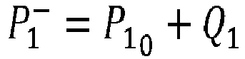
    • obtaining:
    ∘ vehicle motion data stemming from at least one vehicle sensor, and
    ∘ while the GNSS signal is available, GNSS data of a positioning of the vehicle, including a distance variation and an orientation variation, and
    • calibrating parameters of an odometer of the vehicle based on a data fusion that uses a Kalman filter that determines a predicted distance variation and a predicted orientation variation of the vehicle based on a current calibration of the odometer parameters and on the motion data, and that compares the predicted distance variation and predicted orientation variation to the distance variation and the orientation variation of the GNSS data.
  2. The method of claim 1, wherein the odometer predicts cyclically in time a new location of the vehicle and a new heading of the vehicle based on a location and heading predicted at the previous cycle and on the motion data.
  3. The method of claim 2, wherein the motion data includes the vehicle speed in the current cycle, the vehicle speed in the previous cycle, and the vehicle yaw rate in the current cycle.
  4. The method of any one of claims 1 to 3, wherein the parameters of the odometer include a vehicle speed scaling, a vehicle yaw rate scaling, and a vehicle yaw rate offset.
  5. The method of claim 4, wherein calibrating parameters includes correcting one or any combination of the vehicle speed scaling, the vehicle yaw rate scaling, and the vehicle yaw rate offset.
  6. The method of any one of claims 1 to 5, wherein the motion data stems from a wheel sensor, an Inertial Measurement Unit (IMU), and a steering system sensor.
  7. The method of any one of claims 1 to 6, wherein the GNSS data further includes a location and heading of the vehicle, and the method further comprises, in real-time:
    when the GNSS signal is available, determining a localization of the vehicle by performing a data fusion that is based on a Kalman filter that predicts the vehicle localization based on a fusion of the location and heading of the GNSS data and a location and heading predicted according to the calibrated odometer parameters;
    when the GNSS signal is lost, determining a localization of the vehicle based on a location and heading predicted according to the calibrated odometer parameters.
  8. The method of any one of claims 1 to 7, wherein the GNSS data stems from a GNSS device that comprises only one antenna.
  9. The method of any one of claims 1 to 8, wherein the vehicle is a motorbike, a car, a bus or a truck.
  10. A computer program comprising instructions which, when executed by a computer system, cause the system to perform the method of any one of claims 1 to 9.
  11. A computer-readable data storage medium having recorded thereon the computer program of claim 10.
  12. A system comprising a processor coupled to a memory, the memory having recorded thereon the computer program of claim 10.
  13. The system of claim 12, wherein the system is coupled with or further comprises the GNSS device, the odometer, and the at least one sensor.
  14. The system of claim 12, wherein the at least one sensor includes a wheel sensor, an Inertial Measurement Unit (IMU), and a steering system sensor.
  15. A vehicle equipped with the system according to any one of claims 12 to 14.
EP23169054.6A 2023-04-20 2023-04-20 Localizing a moving vehicle Pending EP4450925A1 (en)

Priority Applications (3)

Application Number Priority Date Filing Date Title
EP23169054.6A EP4450925A1 (en) 2023-04-20 2023-04-20 Localizing a moving vehicle
US18/641,112 US20240353578A1 (en) 2023-04-20 2024-04-19 Localizing a moving vehicle
CN202410481467.6A CN118816856A (en) 2023-04-20 2024-04-22 Locating moving vehicles

Applications Claiming Priority (1)

Application Number Priority Date Filing Date Title
EP23169054.6A EP4450925A1 (en) 2023-04-20 2023-04-20 Localizing a moving vehicle

Publications (1)

Publication Number Publication Date
EP4450925A1 true EP4450925A1 (en) 2024-10-23

Family

ID=86096075

Family Applications (1)

Application Number Title Priority Date Filing Date
EP23169054.6A Pending EP4450925A1 (en) 2023-04-20 2023-04-20 Localizing a moving vehicle

Country Status (3)

Country Link
US (1) US20240353578A1 (en)
EP (1) EP4450925A1 (en)
CN (1) CN118816856A (en)

Families Citing this family (1)

* Cited by examiner, † Cited by third party
Publication number Priority date Publication date Assignee Title
US20250189681A1 (en) * 2023-12-06 2025-06-12 Qualcomm Incorporated Enhanced motion state detection for location services

Citations (4)

* Cited by examiner, † Cited by third party
Publication number Priority date Publication date Assignee Title
US5416712A (en) * 1993-05-28 1995-05-16 Trimble Navigation Limited Position and velocity estimation system for adaptive weighting of GPS and dead-reckoning information
EP1096230A2 (en) * 1999-10-29 2001-05-02 Visteon Global Technologies, Inc. Method and apparatus for inertial guidance for an automobile navigation system
EP2541203A1 (en) * 2011-06-30 2013-01-02 Furuno Electric Company Limited Road map feedback server for tightly coupled gps and dead reckoning vehicle navigation
US20160097862A1 (en) * 2014-10-06 2016-04-07 Hyundai Mobis Co., Ltd. System and method for complex navigation using dead reckoning and gps

Family Cites Families (7)

* Cited by examiner, † Cited by third party
Publication number Priority date Publication date Assignee Title
EP1924981B1 (en) * 2005-07-26 2012-09-12 MacDonald Dettwiler & Associates Inc. Traffic management system for a passageway environment
EP2450668B1 (en) * 2010-11-04 2014-01-15 u-blox AG A method for tracking the position and the heading of a vehicle using dead reckoning and a tracking device for carrying out the method
WO2012062339A1 (en) * 2010-11-08 2012-05-18 Elektrobit Automotive Gmbh Technique for calibrating dead reckoning positioning data
US8825397B2 (en) * 2011-11-03 2014-09-02 Texas Instruments Incorporated Vehicle navigation system with dead reckoning
JP5831308B2 (en) * 2012-03-13 2015-12-09 アイシン・エィ・ダブリュ株式会社 Moving body position detection system, moving body position detection apparatus, moving body position detection method, and computer program
KR102014261B1 (en) * 2017-12-12 2019-08-26 엘지전자 주식회사 Vehicle control device mounted on vehicle and method for controlling the vehicle
US12530970B2 (en) * 2018-12-26 2026-01-20 Zoox, Inc. Collision avoidance system

Patent Citations (4)

* Cited by examiner, † Cited by third party
Publication number Priority date Publication date Assignee Title
US5416712A (en) * 1993-05-28 1995-05-16 Trimble Navigation Limited Position and velocity estimation system for adaptive weighting of GPS and dead-reckoning information
EP1096230A2 (en) * 1999-10-29 2001-05-02 Visteon Global Technologies, Inc. Method and apparatus for inertial guidance for an automobile navigation system
EP2541203A1 (en) * 2011-06-30 2013-01-02 Furuno Electric Company Limited Road map feedback server for tightly coupled gps and dead reckoning vehicle navigation
US20160097862A1 (en) * 2014-10-06 2016-04-07 Hyundai Mobis Co., Ltd. System and method for complex navigation using dead reckoning and gps

Non-Patent Citations (1)

* Cited by examiner, † Cited by third party
Title
M. SPECHT: "Experimental Studies on the Relationship Between HDOP and Position Error in the GPS System", METROLOGY AND MEASUREMENT SYSTEMS, vol. 29, no. 1, March 2022 (2022-03-01), pages 17 - 36

Also Published As

Publication number Publication date
CN118816856A (en) 2024-10-22
US20240353578A1 (en) 2024-10-24

Similar Documents

Publication Publication Date Title
EP2519803B1 (en) Technique for calibrating dead reckoning positioning data
JP5855249B2 (en) Positioning device
US10240931B2 (en) System and method for navigation by applying corrected bias values to gyroscopic data
US7286933B2 (en) GPS/dead-reckoning combination system and operating method thereof
US8560234B2 (en) System and method of navigation based on state estimation using a stepped filter
US20150153178A1 (en) Car navigation system and method in which global navigation satellite system (gnss) and dead reckoning (dr) are merged
US9423250B1 (en) Position measurement correction using loop-closure and movement data
CN102466802B (en) Dead reckoning is used to follow the trail of the method at vehicle location and vehicle heading angle and realize the follow-up mechanism of the method
US11650324B2 (en) Navigation apparatus and method in which measurement quantization errors are modeled as states
CN107588769A (en) A kind of vehicle-mounted inertial navigation, odometer and altimeter Combinated navigation method
US11187719B2 (en) In-motion initialization of accelerometer for accurate vehicle positioning
CN115060257B (en) Vehicle lane change detection method based on civil-grade inertia measurement unit
US20240353578A1 (en) Localizing a moving vehicle
CN113063441B (en) Data source correction method and device for accumulated calculation error of odometer
JP6248559B2 (en) Vehicle trajectory calculation device
US20200225059A1 (en) Method for calibrating gyro sensor on basis of vehicle speed
US20050159857A1 (en) System and method for determining aircraft tapeline altitude
KR102250107B1 (en) Device for vehicle speed correction and method of calculating the wheel scale factor by the same
KR101964059B1 (en) System for locating vehicle based on wheel speed sensor for guide system in indoor parking lot
JP5994237B2 (en) Positioning device and program
CN114279439B (en) A method, device and system for correcting inertial navigation data
CN105759292A (en) Method and system for calibrating relative position parameter of differential GPS and robot
EP4451016A1 (en) Determination of the altitude of a moving vehicle
EP4571254A1 (en) Method for the localization of a moving vehicle
RU2830723C1 (en) Method of determining trajectory of object in surrounding space for constructing 3d map

Legal Events

Date Code Title Description
PUAI Public reference made under article 153(3) epc to a published international application that has entered the european phase

Free format text: ORIGINAL CODE: 0009012

STAA Information on the status of an ep patent application or granted ep patent

Free format text: STATUS: THE APPLICATION HAS BEEN PUBLISHED

AK Designated contracting states

Kind code of ref document: A1

Designated state(s): AL AT BE BG CH CY CZ DE DK EE ES FI FR GB GR HR HU IE IS IT LI LT LU LV MC ME MK MT NL NO PL PT RO RS SE SI SK SM TR

STAA Information on the status of an ep patent application or granted ep patent

Free format text: STATUS: REQUEST FOR EXAMINATION WAS MADE

17P Request for examination filed

Effective date: 20250410