EP4334740B1 - Verfahren zur zweidimensionalen und dreidimensionalen bildgebung auf der basis von benachbarten radaren mit mehreren eingängen und mehreren ausgängen - Google Patents
Verfahren zur zweidimensionalen und dreidimensionalen bildgebung auf der basis von benachbarten radaren mit mehreren eingängen und mehreren ausgängen Download PDFInfo
- Publication number
- EP4334740B1 EP4334740B1 EP22726140.1A EP22726140A EP4334740B1 EP 4334740 B1 EP4334740 B1 EP 4334740B1 EP 22726140 A EP22726140 A EP 22726140A EP 4334740 B1 EP4334740 B1 EP 4334740B1
- Authority
- EP
- European Patent Office
- Prior art keywords
- frequency
- target
- fft
- delay
- hula
- Prior art date
- Legal status (The legal status is an assumption and is not a legal conclusion. Google has not performed a legal analysis and makes no representation as to the accuracy of the status listed.)
- Active
Links
Images













Classifications
-
- G—PHYSICS
- G01—MEASURING; TESTING
- G01S—RADIO DIRECTION-FINDING; RADIO NAVIGATION; DETERMINING DISTANCE OR VELOCITY BY USE OF RADIO WAVES; LOCATING OR PRESENCE-DETECTING BY USE OF THE REFLECTION OR RERADIATION OF RADIO WAVES; ANALOGOUS ARRANGEMENTS USING OTHER WAVES
- G01S7/00—Details of systems according to groups G01S13/00, G01S15/00, G01S17/00
- G01S7/02—Details of systems according to groups G01S13/00, G01S15/00, G01S17/00 of systems according to group G01S13/00
- G01S7/35—Details of non-pulse systems
- G01S7/352—Receivers
- G01S7/354—Extracting wanted echo-signals
-
- G—PHYSICS
- G01—MEASURING; TESTING
- G01S—RADIO DIRECTION-FINDING; RADIO NAVIGATION; DETERMINING DISTANCE OR VELOCITY BY USE OF RADIO WAVES; LOCATING OR PRESENCE-DETECTING BY USE OF THE REFLECTION OR RERADIATION OF RADIO WAVES; ANALOGOUS ARRANGEMENTS USING OTHER WAVES
- G01S13/00—Systems using the reflection or reradiation of radio waves, e.g. radar systems; Analogous systems using reflection or reradiation of waves whose nature or wavelength is irrelevant or unspecified
- G01S13/02—Systems using reflection of radio waves, e.g. primary radar systems; Analogous systems
- G01S13/06—Systems determining position data of a target
- G01S13/08—Systems for measuring distance only
- G01S13/32—Systems for measuring distance only using transmission of continuous waves, whether amplitude-, frequency-, or phase-modulated, or unmodulated
- G01S13/34—Systems for measuring distance only using transmission of continuous waves, whether amplitude-, frequency-, or phase-modulated, or unmodulated using transmission of continuous, frequency-modulated waves while heterodyning the received signal, or a signal derived therefrom, with a locally-generated signal related to the contemporaneously transmitted signal
- G01S13/345—Systems for measuring distance only using transmission of continuous waves, whether amplitude-, frequency-, or phase-modulated, or unmodulated using transmission of continuous, frequency-modulated waves while heterodyning the received signal, or a signal derived therefrom, with a locally-generated signal related to the contemporaneously transmitted signal using triangular modulation
-
- G—PHYSICS
- G01—MEASURING; TESTING
- G01S—RADIO DIRECTION-FINDING; RADIO NAVIGATION; DETERMINING DISTANCE OR VELOCITY BY USE OF RADIO WAVES; LOCATING OR PRESENCE-DETECTING BY USE OF THE REFLECTION OR RERADIATION OF RADIO WAVES; ANALOGOUS ARRANGEMENTS USING OTHER WAVES
- G01S7/00—Details of systems according to groups G01S13/00, G01S15/00, G01S17/00
- G01S7/02—Details of systems according to groups G01S13/00, G01S15/00, G01S17/00 of systems according to group G01S13/00
- G01S7/35—Details of non-pulse systems
- G01S7/352—Receivers
- G01S7/356—Receivers involving particularities of FFT processing
Definitions
- the present invention relates to a deterministic method for the detection of multiple targets and the estimation of their spatial coordinates in a colocated multiple-input multiple-output radar system operating in a slowly changing two-dimensional or three-dimensional propagation scenario.
- Two specific embodiments of the proposed method are described in detail for both frequency modulated continuous wave radars (FMCW) and stepped frequency continuous wave (SFCW) radars. These embodiments have, among others, the following relevant features:
- the second feature make them computationally efficient. Moreover, the first embodiment and part of the second embodiment lend themselves to an efficient implementation on parallel hardware platforms. Specific technical problems experienced in the implementation of the proposed embodiments on commercial radar devices are identified and possible solutions are proposed. Our numerical results lead to the conclusion that the described embodiments are able to generate accurate radar images in the presence of multiple and closely spaced targets.
- Low cost commercial radar devices can be used to implement the present invention.
- MIMO radar systems can be divided in statistical MIMO radars and colocated MIMO radars on the basis of the distance between their transmit array and their receive array; in the first case, transmit and receive antennas are widely separated, whereas, in the second one, they are closely spaced and, in particular, they are usually placed on the same shield.
- transmit and receive antennas are widely separated, whereas, in the second one, they are closely spaced and, in particular, they are usually placed on the same shield.
- colocated MIMO radars only; such systems play an important role in a number of applications, because of their limited cost, their small size and their ability to detect the presence of multiple targets.
- any colocated MIMO radar system depends not only on some important characteristics of its hardware (e.g., the operating frequency, the number of transmit and receive antennas, the configuration of the transmit and receive arrays, etc.), but also on the techniques that are employed in the generation of its radiated waveforms and in the processing of the measurements acquired through its receive array.
- optimal i.e., maximum likelihood, ML
- ML maximum likelihood
- target delays are first estimated by applying the multiple signal classification (MUSIC) algorithm to a temporal auto-correlation matrix or by identifying the beat frequencies in the downconverted received signal through spectral analysis (more specifically, through the FFT algorithm) in the solution proposed by Oh and in that proposed by Lin, respectively; then, the acquired information are exploited to estimate the DOA of the echoes originating from the detected targets.
- MUSIC multiple signal classification
- the parameters of the dominant target are estimated first; then, its contribution to the received signals is cancelled and the resulting residual signals are processed to detect the next dominant target. This detection/estimation/cancellation procedure is iterated until no significant target is detected on the basis of the residual signals.
- the present solution shares some important features with the detection/estimation techniques developed in Lin and Sirignano. Indeed, similarly as the techniques illustrated in Sirignano, the present method is deterministic, it processes a single snapshot, operates in an iterative fashion and is computationally efficient; its last feature can be related to the fact it requires the evaluation of 1D FFTs only and the search for the global maximum of proper cost functions over 1D (frequency, azimuth or elevation) domains. Moreover, similarly to Lin, it first extracts the range of each detected target from the spectra of the received signals and, then, fuses the information originating from such spectra to extract direction of arrival (DOA) information. However, unlike the methods developed in prior art, it can be employed in both FMCW and SFCW radar systems.
- DOA direction of arrival
- the present solution involve the following concepts:
- second element does not imply the presence of a "first element”, first, second, etc.. are used only for improving the clarity of the description and they should not be interpreted in a limiting way.
- RF radio frequency
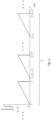
- a ramp generator feeds a voltage controlled oscillator (VCO), that produces a chirp frequency modulated signal, whose instantaneous frequency evolves periodically, as illustrated in Figure 2 ;
- VCO voltage controlled oscillator
- T, T R and T 0 represent the chirp interval, the reset time and the pulse period (or pulse repetition interval), respectively
- f 0 and B are the so called start frequency and the bandwidth, respectively, of the frequency modulated signal.
- the FM signal feeds a power amplifier whose response is sent to one of the N T available transmit (TX) antennas.
- TX transmit
- TDM time division multiplexing
- TX antenna, RX antenna TX antenna
- RX antenna RX antenna
- N VR N T ⁇ N R elements.
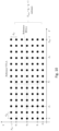
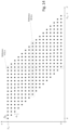
- N ULA horizontal uniform linear arrays ULAs
- N VR N ULA ⁇ N EL . Additional details about this technical issue can be found, for example, in Sirignano.
- the sequence ⁇ w v,n ⁇ consists of zero mean and independent Gaussian random variables, each having variance ⁇ w 2 .
- the frequency downconversion of the received RF signals entails the extraction of both the inphase and quadrature components of each of such signals.
- the maximum target delay ⁇ M (i.e., the maximum resolvable frequency) depends on the sampling frequency f s adopted in the analog-to-digital conversion since aliasing must be avoided; more specifically, it is not difficult to show that the inequality ⁇ M ⁇ f s 2 ⁇ must be satisfied.
- the transmitted signal allows to sound the communication channel between the TX and each of the RX antennas at the N equally spaced frequencies expressed by eq. (1.20). For this reason, the processing accomplished at the receive side of the radar system aims at generating an estimate of the channel frequency response at each of these frequencies.
- these estimates are collected in the vector x p , q ⁇ x 0 p q , x 1 p q , ... , x N ⁇ 1 p q T , that refers to the RVA identified by the horizontal index p and the vertical index q (and denoted ( p,q ) RVA or v-th RVA);
- the equivalent notation x v ⁇ x v , 0 , x v , 1 , ... , x v , N ⁇ 1 T can be also adopted, where v is a single index related with the couple ( p,q ) through a specific one-to-one mapping.
- the sequence ⁇ w v,n ⁇ consists of zero mean and independent complex Gaussian random variables, each having variance ⁇ w 2 .
- the first term appearing in the right-hand side (RHS) of eq. (1.23) represents the frequency response of the communication channel associated with the v -th RVA at the frequency f n (1.20). It is also worth noting that eq.
- the former model is complex, whereas the latter one is real. This difference has to be kept carefully into account in our description of the detection/estimation techniques illustrated in the following section.
- each vector of the set ⁇ r v ⁇ ( ⁇ x v ⁇ ; see eqs. (1.6) and (1.22), respectively) undergoes FFT processing, so that signal analysis is moved from the time-domain (frequency-domain) to the frequency-domain (time-domain) in a FMCW (SFCW) radar system.
- the FFT output is processed by a range profile estimator (RPE); this generates an estimate of the target range profile (TRP), i.e.
- SPE spatial estimator
- the processing accomplished in the first embodiment of the proposed method is described by the block diagram illustrated in Fig. 5 and can be divided in three tasks, each associated with one of the blocks appearing in that figure (the i-th task is denoted T i in the following).
- DFT N 0 [x] denotes, up to a scale factor, the N 0 -th order discrete Fourier transform
- T2 RPE -
- the aim of this task is generating a preliminary estimate of the number of targets and of their ranges. Note that, in this step, multiple targets having the same range or ranges whose difference is below the range resolution of the employed radar system are detected as a single target and no effort is made to separate their contributions.
- the processing accomplished within this task involves N A of the N VR RVAs and consists of three consecutive steps listed below (the i-th step is denoted T2-Si in the following); each step is associated with one of the blocks contained in the RPE block appearing in Figure 7 .
- the selected triads are denoted ⁇ ( X 0, v , X 1, v , X 2, v ); v ⁇ ⁇ , where is the set of the values of the index v identifying them.
- Target detection and range estimation - This step aims at detecting the most relevant targets on each of the N A antennas selected in the previous step and at estimating their ranges (i.e., the frequencies associated with these ranges; see eqs. (1.7) and (1.9)) and their complex amplitudes (see eq. (1.18)).
- the processing accomplished within it is executed on an antenna-by-antenna basis and exploits a novel iterative estimation algorithm called single target detection, range estimation and cancellation (STDREC) and whose detailed description is provided in the Paragraph 4.1.
- STDREC-S1 Detection of a new target and estimation of its parameters -
- the triad X 0 , v k i X 1 , v k i X 2 , v k i is processed to detect a new (i.e., the i-th) target, and to estimate the frequency f v k i and the complex amplitude C v k i associated with it.
- the processing accomplished in this step is executed by an algorithm, dubbed single frequency estimator (SFE) if the received sequence ⁇ r v,n ⁇ is real and complex single frequency estimator (CSFE) if the received sequence ⁇ r v,n ⁇ is complex; this algorithm represents the most important part of the STDREC algorithm and is described in detail in Paragraph 4.1.2 if the received sequence ⁇ r v,n ⁇ is real and in Paragraph 4.1.3 if the received sequence ⁇ r v,n ⁇ is complex.
- SFE single frequency estimator
- CSFE complex single frequency estimator
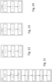
- Steps 3.1.1 and 3.1.2 of Figure 22 can be replaced by an alternative method including (see Steps 3.2.1 - 3.2.2 of Figure 23 ):
- Step 3 of Figure 21 includes (see Steps 3.3.0 - 3.3.2 of Figure 24 ):
- Steps 3.3.1 and 3.3.2 of Figure 24 can be replaced by an alternative method including (see Steps 3.4.1 - 3.4.2 of Figure 25 ):
- STDREC-S2 Cancellation of the new target -
- Step 4 of Figure 21 includes the computation and subtraction of the contribution given by said dominant target to said spectrum ( X ⁇ 0 v ) and to the corresponding derivatives to compute a residual of the spectrum and of the corresponding derivatives.
- the cardinality L b of the last set represents a preliminary estimate of the overall number of targets; this is due to the fact that the energy associated with a given bin may originate from multiple targets, characterized by similar ranges.
- Step 6 of Figure21 can be described as follows (see Steps 6.1 - 6.2 of Figure 26 ):
- the SPE can be implemented independently from the RPE.
- the RPE represents an inventive method for the estimation of ranges, but, in the implementation of the SPE any known method, such as the periodogram method as in “ J. Selva, "ML Estimation and Detection of Multiple Frequencies Through Periodogram Estimate Refinement", IEEE Signal Processing Letters, vol. 24, n. 3, pagg. 249-253, mar. 2017 " and references therein, for the estimation of the ranges can be implemented to feed the SPE.
- RPE can be implemented independently from SPE, being possible to estimate angles from the ranges estimated by RPE, using known techniques, such as 2D FFT processing over the whole receive array as described in " S. Rao, "MIMO Radar,” Texas Instruments - Application Report SWRA554A, July 2018 , for FMCW radar systems”.
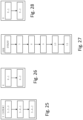
- Said execution (see Step 10 of Figure 27 ) for the first embodiment is carried out by running multiple parallel processes whose number is equal to the number of said frequency bins of said acquired list and said generation of the overall image (Step 11 of Figure 27 ) is carried out when all parallel processes have been executed.
- each of the L b frequency bins identified by the RPE are analysed in the angular (i.e., in the azimuth-elevation) domain.
- This allows to: a) estimate the angular coordinates (i.e., azimuth and elevation) of the target or of the targets whose frequencies (i.e., ranges) fall inside each bin of the set (2.23); b) detect additional targets associated with adjacent frequency bins; c) estimate the angular coordinates (i.e., azimuth and elevation) and compute a finer estimate of the range of such additional targets.
- the above mentioned acquisition includes (see Steps 8.1 - 8.2 of Figure 28 ):
- the processing accomplished within this task consists of the two consecutive steps listed below (the i-th step is denoted T3-Si in the following); each step is associated with one of the blocks contained in the SPE block appearing in Figure 7 .
- the l -th estimator executes a novel recursive estimation algorithm, called single target detection, angular estimation and cancellation (STDAEC) and whose description is provided below (additional details can be found in Paragraph 4.1).
- STDAEC single target detection, angular estimation and cancellation
- the estimates of the parameters ⁇ i [ l ], ⁇ i [ l ], R i [ l ] and C i [ l ] computed by the STDAEC are denoted ⁇ i [ l ], ⁇ i [ l ], R ⁇ i [ l ] and ⁇ i [ l ], respectively.
- the derivation of the STDAEC algorithm relies on the fact that the i -th target provides an additive contribution to all the elements of the matrix X [ l ] (2.24) and that the phase of this contribution exhibit periodic variations as we move horizontally or vertically along this matrix. More specifically, if we assume that the intensity of the echo received by each RVA from the i- th target does not change from antenna to antenna, the complex amplitude C i [ p, q, l ] associated with the i -th target detected in the l -th frequency bin and observed on the ( p , q ) RVA (i.e., contributing to the spectral coefficient X l [ p, q ]; see eqs.
- the rate of the phase variations observed in the complex amplitudes ⁇ C i [ p, q, l ] ⁇ as we move horizontally along the considered virtual receive array is proportional to the quantity F H , i l ⁇ 2 d VH ⁇ cos ⁇ i l sin ⁇ i l
- the rate of the phase variations observed in the same amplitudes as we move vertically along the same array is proportional to F V , i l ⁇ 2 d VV ⁇ sin ⁇ i l .
- the horizontal and vertical spatial frequencies can be detected by first computing a 2D DFT of the matrix X [ l ] (2.24) and, then, by looking for the local maxima of the absolute values of the elements of the resulting 2D matrix; note that the matrix X [ l ] can be also zero-padded before computing its 2D FFT to improve spectral resolution.
- 2D processing is avoided by alternating vertical and horizontal 1D DFT processing; consequently, relevant spatial frequencies are estimated by searching for the peaks of 1D amplitude spectra (in other words, an AM approach is adopted).
- the following two additional techniques are exploited:
- folding generates a single folded spectrum and has the beneficial effects of a) averaging the effects of the noise affecting different RVAs and b) combining in an unconstructive fashion the contributions of all the targets different from the one which the employed spatial frequencies refer to. For this reason, in analysing the amplitude of the folded spectrum, a well defined peak in its amplitude is expected in l -th frequency bin or in a bin close to it. However, if this does not occur, the detected target is actually a false target (i.e., a ghost target ). If a peak exists, its position allows to compute a refined estimate of the frequency (and, consequently, of the range) characterizing the target for which folding has been accomplished.
- the whole virtual receive array or a subset of it can be used.
- the exploitation of a subset of the available RVAs is motivated by the fact that, in practice, in computing folded spectra, the estimates F ⁇ H,i [ l ] and F ⁇ V,i [ l ] of the frequencies F H,i [ l ] and F V,i [ l ], respectively, are employed and that estimation errors may substantially affect the quality of the phase compensation factors computed for the antennas that are farther from the reference antenna or the reference horizontal/vertical ULA.
- the selection includes:
- the STDAEC algorithm starts executing its iterations. Within its i-th iteration, it accomplishes the three steps described below.
- the N VH ⁇ N VV matrix X i l ⁇ X l i p q is processed to detect the strongest target contributing to it, and to estimate the angular parameters ( ⁇ i [ l ], ⁇ i [ l ]) and the complex amplitude C i [ l ] associated with it (this target represents the i- th one detected in the considered frequency bin, since ( i - 1) targets have been detected in the previous recursions).
- STDAE single target detection and angular estimation
- the processing accomplished within this step is based on a novel iterative detection and estimation algorithm called single target detection and angular estimation (STDAE) and whose detailed description is provided in Paragraph 4.1; this algorithm consists in the five steps described below (its r -th step is denoted STDAE-S r in the following).
- STDAE-S r the first three steps (i.e., STDAE-S1 to STDAE-S3) have not to be performed; therefore, the first step to be carried out is STDAE-S4.
- the matrix X ( i ) [ l ] (2.31) is replaced with the N VH -dimensional vector X i l ⁇ X l i p ,
- said estimation includes a preliminary step (Step 10.1.0) including:
- STDAE-S1 FFT processing on the reference VULA -
- STDAE-S2 Single angle estimation -
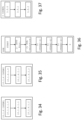
- Step 10.1.2 of Figure 29 the method for the estimation of the vertical spatial frequency (see Step 10.1.2 of Figure 29 ) can be described as follows (see Steps 10.1.2.1.0 - 10.1.2.1.2 of Figure 30 ):
- Steps 10.1.2.1.1 - 10.1.2.1.2 of Figure 30 can be replaced by an alternative method including (see Steps 10.1.2.2.1 - 10.1.2.2.2 of Figure 31 ):
- phase rotation factor R i VF l q ⁇ exp ⁇ j ⁇ i VF l q ⁇ q R , with ⁇ i VF l ⁇ 2 ⁇ ⁇ F ⁇ V , i l , is computed for the q-th HULA (with q q I VF , q I VF + 1 , ... , q R ⁇ 1 , q R + 1 , ... , q F VF ).
- STDAE-S4 FFT processing and horizontal frequency estimation -
- the processing accomplished in this step is very similar to that carried out in STDAE-S1 and STDAE-S2.
- the only difference is represented by the fact that the N VULA -dimensional vector X VULA i l (2.33) is replaced by the N HULA -dimensional vector X i VF l (2.45) generated in the previous step if the STDAE algorithm is used for 3D imaging and by the vector X ( i ) [ l ] (2.32) if the STDAE algorithm is used for 2D imaging.
- the CSFE is exploited to estimate the horizontal frequency F H,i [ l ] and, again, the complex amplitude A i [ l ] associated with the i-th target.
- Step 10.1.5 of Figure 29 the method for the estimation of the horizontal spatial frequency (see Step 10.1.5 of Figure 29 ) can be described as follows (see Steps 10.1.5.1.0 - 10.1.5.1.2 of Figure 32 ):
- Steps 10.1.5.1.1 - 10.1.5.1.2 of Figure 32 can be replaced by an alternative method including (see Steps 10.1.5.2.1 - 10.1.5.2.2 of Figure 33 ):
- a relative maximum i.e., a peak
- the SFE algorithm is run to estimate, on the basis of the vectors X 0,OF [ l ], X 1,OF [ l ] and X 2,OF [ l ] (see eq.
- the final estimates f ⁇ i l ⁇ ⁇ i l f DFT + ⁇ ⁇ i l f DFT , and ⁇ i [ l ] of the parameters f i [ l ] and A i [ l ] characterizing the i -th target detected in the l -th frequency bin.
- the integer part ⁇ i [ l ] of the frequency f ⁇ i [ l ] does not necessarily coincide with ⁇ l (see eq. (2.54)); however, if it differs, it is close to ⁇ l .
- Said checking is performed on the absolute value of said overall folded spectrum ( X OF ,0 ).
- Step 10.1.6 of Figure 29 the method for the refinement (see Step 10.1.6 of Figure 29 ) can be described as follows (see Steps 10.1.6.1.0 - 10.1.6.1.2 of Figure 34 ):
- Steps 10.1.6.1.1 - 10.1.6.1.2 of Figure 34 can be replaced by an alternative method including (see Steps 10.1.6.2.1 - 10.1.6.2.2 of Figure 35 ):
- D [ l ] iterations are accomplished by the STDAEC algorithm operating on the ⁇ l -th frequency bin, no more than D [ l ] distinct targets are identified in that bin ( D [ l ] targets are found if none of them is deemed to be a ghost target).
- the STDAEC algorithm can be easily extended in a way that multiple angles are detected and estimated in parallel. This means that multiple instances of the CSFE algorithm are run in parallel.
- T3-S2 Evaluation of spatial coordinates and generation of the overall image -
- This task aims at: a) computing the spatial coordinates of all the targets on the basis of the spatial information generated by the L b STDAEC algorithms and collected in the L b sets ⁇ ⁇ (see eq. (2.59)); b) generating the overall image of the propagation scenario. More specifically, the estimates of the range, of the elevation and of the azimuth of the i-th target detected in the ⁇ l -th frequency bin are computed as (see eqs.
- the processing accomplished in the second embodiment of the proposed method is described by the block diagram illustrated in Figure 12 and can be divided in three tasks, each associated with one of the blocks appearing in that figure (the i -th task is denoted T i in the following). In all these tasks, a single array snapshot is processed. The first two tasks of this embodiment (namely, those concerning FFT processing and RPE) coincide with that of the first embodiment. For this reason, in the remaining part of this paragraph, the third task only is sketched; additional details about the algorithms employed in this task are provided in Paragraph 4.2.
- said acquisition includes the acquisition of target energy and wherein said execution (see Step 10 of Figure 27 ) is repeated sequentially over the acquired list, ordered according to said target energy, and wherein said generation of the overall image (Step 11 of Figure 27 ) is carried out when all the frequency bins have been analyzed.
- a refined estimate of the range for all the targets detected in the considered frequency bin is computed on the basis of set of triads X 0 , v l , X 1 , v l , X 2 , v l . Then, the estimates of the range and of the angular parameters of the D [ l ] detected targets are: a) made available at the output of the SPE; b) processed by another algorithm, called single bin cancellation (SBC).
- SBC single bin cancellation
- the SBC algorithm estimates the contributions C X 0 , v l C X 1 , v l C X 2 , v l of these targets (i.e., of the l -th frequency bin) to the set of triads X 0 , v l , X 1 , v l , X 2 , v l (see eqs. (4.11)-(4.13)) and cancels it.
- a similar adaptation for 2D imaging can be derived also for the second embodiment since it is based on the same algorithms adopted in the first one.
- said cancellation includes the computation and subtraction of the contribution given by said dominant point target to said spectrum ( X ⁇ 0 v ) and to the corresponding derivatives to generate a new residual of the spectrum and of the corresponding derivatives.
- T2 The changes to be made in T2 concern its second step (i.e., the STDREC algorithm), since the noisy measurements processed in this step are always complex (see eqs. (1.22)-(1.23)); the new structure of this step is summarized below.
- T2-S2 Target detection and range estimation - In this step, that aims at detecting the most relevant targets on each of the N A antennas, a minor change is required in the cancellation procedure with respect to its counterpart employed in the MIMO FMCW radar system. This is due to the fact that, as already stated above, the noisy measurements processed in a MIMO SFCW radar system are always represented by complex (frequency-domain) sequences.
- the delay ⁇ v k i and the complex amplitude A v k i associated with the i-th target are estimated.
- Step 3 of Figure 36 includes (see Steps 3.5.0 - 3.5.2 of Figure 37 ):
- Steps 3.5.1 and 3.5.2 of Figure 37 can be replaced by an alternative method including (see Steps 3.6.1 - 3.6.2 of Figure 38 ):
- Step 4 of Figure 36 includes the computation and subtraction of the contribution given by said dominant target to said impulse response ( X ⁇ 0 v ) and to the corresponding derivatives to compute a residual of the impulse response and of the corresponding derivatives.
- the vector X 0 , v k can be seen as a collection of noisy information referring to N 0 distinct delay bins (i.e., to N 0 distinct range bins) and is usually dense in the presence of multiple extended targets.
- the STDREC allows to extract a discrete delay (i.e., range) profile from the vector X 0, v k ; such a profile is usually sparse.
- the final output of the information fusion is represented by the set (2.23). Note that the cardinality L b of the last set represents a preliminary estimate of the overall number of targets.
- Step 6 of Figure 36 can be described as follows (see Steps 6.1 - 6.2 of Figure 26 ):
- the SPE can be implemented independently from the RPE.
- the RPE represents an inventive method for the estimation of ranges, but, in the implementation of the SPE any known method, such as the periodogram method, for the estimation of the ranges can be implemented to feed the SPE.
- RPE can be implemented independently from SPE, being possible to estimate angles from the ranges estimated by RPE, using known techniques, such as 2D IFFT processing over the whole receive array.
- Said execution (see Step 10 of Figure 27 ) for the first embodiment is carried out by running multiple parallel processes whose number is equal to the number of said delay bins of said acquired list and said generation of the overall image (Step 11 of Figure 27 ) is carried out when all parallel processes have been executed.
- step T3 The processing accomplished in T3 (i.e., by the SPE) has the same structure and interpretation as that illustrated for the FMCW radar system since it aims at estimating the angular parameters of the targets on the basis of the discrete range profile computed in T2.
- frequency bins are now replaced by delay bins and, consequently, the normalised horizontal and vertical frequencies F H,i and F V,i by the normalised horizontal and vertical delays T H,i and T V,i , respectively.
- step T3-S1 the matrix X [ l ] is still defined on the basis of eq. (2.24), but the complex amplitude A i [ p,q,l ] appearing in eq. (2.25) is replaced by (see eqs.
- a i p q l A i l exp ⁇ j 4 ⁇ ⁇ d VH p ⁇ p R cos ⁇ i l sin ⁇ i l + d VV q ⁇ q R sin ⁇
- a i [ l ] is the complex amplitude observed for the i -th target in the l -th time bin on the reference RVA.
- the above mentioned acquisition includes (see Steps 8.1 - 8.2 of Figure 28 ):
- the selection (see Step 9 of Figure 27 ) includes:
- Step 10.1.0 includes:
- Step 10.1.2 of Figure 29 the method for the estimation of the vertical spatial frequency (see Step 10.1.2 of Figure 29 ) can be described as follows (see Steps 10.1.2.1.0 - 10.1.2.1.2 of Figure 39 ):
- Steps 10.1.2.1.1 - 10.1.2.1.2 of Figure 39 can be replaced by an alternative method including (see Steps 10.1.2.2.1 - 10.1.2.2.2 of Figure 40 ):
- STDAE-S3 Vertical folding - Vertical folding is employed to compensate for the phase differences between the considered HULAs.
- the phase rotation factor appearing in eq. (2.45) is computed as R i VF l q ⁇ exp j ⁇ i VF l q ⁇ q R , where ⁇ i VF l ⁇ 2 ⁇ ⁇ T ⁇ V , i l and T ⁇ V,i [ l ] is an estimate of the normalized vertical delay T V,i [ l ] (evaluated in STDAE-S2 ).
- Step 10.1.5 of Figure 29 the method for the estimation of the horizontal spatial frequency (see Step 10.1.5 of Figure 29 ) can be described as follows (see Steps 10.1.5.1.0 - 10.1.5.1.2 of Figure 41 ):
- Steps 10.1.5.1.1 - 10.1.5.1.2 of Figure 41 can be replaced by an alternative method including (see Steps 10.1.5.2.1 - 10.1.5.2.2 of Figure 42 ):
- (2.51) is defined as: R i HF l p ⁇ exp j ⁇ i HF l p ⁇ p R , where ⁇ i HF l ⁇ 2 ⁇ ⁇ T ⁇ H , i l .
- the CSDE algorithm is run to estimate, on the basis of the vectors X 0,OF [ l ], X 1,OF [ l ] and X 2,OF [ l ], the final estimates ⁇ i [ l ] and ⁇ i [ l ] of the parameters ⁇ i [ l ] and A i [ l ] characterizing the i -th target detected in the l -th delay bin. Then, if the estimated delay ⁇ i [ l ] (see eq.
- Said checking is performed on the absolute value of said folded impulse response ( X OF ,0 ).
- Step 10.1.6 of Figure 29 the method for the refinement (see Step 10.1.6 of Figure 29 ) can be described as follows (see Steps 10.1.6.1.0 - 10.1.6.1.2 of Figure 43 ):
- Steps 10.1.6.1.1 - 10.1.6.1.2 of Figure 43 can be replaced by an alternative method including (see Steps 10.1.6.2.1 - 10.1.6.2.2 of Figure 44 ):
- said cancellation includes the computation and subtraction of the contribution given by said dominant point target to the impulse response contribution referred to said considered delay bin to generate a new residual of the impulse response and of the corresponding derivatives.
- STDAEC-S3 Residual energy test -
- the energy E ( i +1) [ l ] of the residual X ( i +1) [ l ] evaluated in the previous step is computed on the basis of eq. (2.58)) and is compared with a positive threshold; if this energy is below this threshold, the STDAEC algorithm stops, otherwise the recursion index i is increased by one and a new iteration is started by going back to STDAEC-S1.
- the processing accomplished in the second embodiment of the proposed method and described by the block diagram illustrated in Figure 12 can be easily adapted to a MIMO SFCW radar system; most of the required changes are the same as those illustrated in the previous paragraph for the embodiment #1.
- the vector r v (1.6) is replaced by the vector x v (1.22), the FFT operation by the IFFT operation, frequency bins by delay bins in the STDREC and STDAEC algorithms (and, consequently, the spatial frequencies F V,i [ l ] and F H,i [ l ] by the normalised delays T V,i [ l ] and T H,i [ l ] , respectively) and the estimation of the complex amplitude A i [ p,l ] observed on the p -th RVA by the estimation of the complex gain A i [ p,l ] (see Paragraph 2.3.1.
- Embodiment #1 Another important change concerns the SBC procedure and, in particular, the evaluation of the triad C X 0 , v l C X 1 , v l C X 2 , v l appearing in eq. (2.68). In fact, the computation of these vectors is based on eqs. (4.238)-(4.240) (see Paragraph 4.2.2), that are different from eqs. (4.232)-(4.234) employed in a MIMO FMCW radar system. Concerning 2D imaging, a similar adaptation can be derived also for a SFCW radar system for both embodiments.
- said acquisition includes the acquisition of target energy and wherein said execution (see Step 10 of Figure 27 ) is repeated sequentially over the acquired list, ordered according to said target energy, and wherein said generation of the overall image (Step 11 of Figure 27 ) is carried out when all the delay bins have been analyzed.
- Said cancellation includes the computation and subtraction of the contribution given by said dominant point target to said impulse response ( X ⁇ 0 v ) and to the corresponding derivatives to generate a new residual of the impulse response and of the corresponding derivatives.
- This problem that affects the data collected through both FMCW and SFCW radar systems, can be mitigated by enriching the physical array with a set of surrounding passive antennas; in this case, the array is artificially extended with new antennas along all its sides, so that the behavior of all its active antennas becomes more uniform.
- the block diagram illustrated in is replaced by that shown in Figure 15 .
- the STDAEC block is replaced by a new block, that implements a new algorithm, called deep STDAEC (DSTDAEC).
- DSTDAEC deep STDAEC
- the initialization procedure of the DSTAEC is the same of the STDAEC and consists in:
- DSTDAEC-S1 Detection of a new target and estimation of its angular parameters -
- This step is identical to the first step of the STDAEC technique. Therefore, the N VH ⁇ N VV matrix X ( i ) [ l ] (see eq. (2.31)) is processed to detect the strongest target (i.e., the i -th target) contributing to the l -th frequency bin and to estimate its parameters ( ⁇ i [ l ], ⁇ i [ l ] ,f i [ l ] ,A i [ l ]). Moreover, the processing accomplished within this step is based on the STDAE algorithm, whose detailed description is provided in Paragraph 2.2.1. Embodiment #1.
- DSTDAEC-S2 Estimation of the distorted amplitudes -
- a deep neural network is employed to predict the absolute value 2 of C ⁇ i [ v , l ] (i.e., to predict a new estimate
- This network is designed to solve a regression problem through a supervised learning approach.
- the architecture proposed for the deep neural network and illustrated in Figure 16 has been inspired by that of feed-forward neural networks (see Chapter 5 of “C. M. Bishop, Pattern Recognition and Machine Learning, ser. Information Science and Statistics. New York, NY: Springer, 2006 .”).
- This architecture is characterized by input and output layers of the same size ( N VR ) and K hidden layers.
- Each layer is composed by neurons and each neuron provides a non-linear combination of its inputs to the next layer.
- the amount of layers and neurons in the network are hyperparameters that they can be freely chosen, so that the weights and bias in each neuron can be optimized. Note, however, that the size of each layer decreases from the input layer to the output layer (see " A. Romero, N. Ballas, S. E. Kahou, A.
- the network has the ability to tune its parameters in order to learn a compressed representation of the input data, so generating an estimate of the amplitude distortion ⁇ v ( ⁇ , ⁇ ).
- DSTDAEC-S4 Residual energy test -
- the energy E (i +1) [ l ] (2.58) of the residual spectrum vector X ( i +1) [ l ] (2.57) (see STDAEC-S3 ) is compared with the positive threshold T STDAEC . If this energy is below the threshold, the DSTDAEC algorithm stops; otherwise, the recursion index i is increased by one and a new iteration is started by going back to DSTDAEC-S1.
- the method for amplitude compensation illustrated for the embodiment #1 can be easily adapted to the embodiment #2 (see Figure 12 ).
- the STDAEC technique is replaced by the DSTDAEC technique.
- the above methods for a MIMO FMCW radar can be described as follows: said compensation of the amplitude distortion (see Step 10.1.7 of Figure 29 ) is carried out employing a deep neural network designed to solve a regression problem through a supervised learning approach wherein network training is based on a dataset collecting the amplitude of a number of said point targets; the compensation of the complex amplitude is carried out by multiplying said refined estimate of the complex amplitude (see Step 10.1.6 of Figure 29 ) by said estimated amplitude distortion for each of said virtual antennas.
- the above methods for a MIMO SFCW radar can be described as follows: said compensation of the amplitude distortion (see Step 10.1.7 of Figure 29 ) is carried out employing a deep neural network designed to solve a regression problem through a supervised learning approach wherein network training is based on a dataset collecting the amplitude of a number of said point targets; the compensation of the complex amplitude is carried out by multiplying said refined estimate of the complex amplitude (see Step 10.1.6 of Figure 29 ) by said estimated amplitude distortion for each of said virtual antennas.
- the array structure illustrated in Figure 14 influences the vertical folding procedure since it involves VULAs of different sizes. More specifically, in the i -th iteration of the STDAEC algorithm vertical folding is accomplished by computing the N HULA -dimensional vector (see the definition (2.31) and STDAE-S3 )
- X i VF l X i VF p I l , X l i p I + 1 , l , ... , X l i p F l T
- the first step of T2 aims at selecting N A distinct RVAs within the set of the N VR available RVAs.
- the SFE computes an estimate f ⁇ x of the frequency f x and an estimate ⁇ of the complex amplitude C ⁇ 1 2 a exp j ⁇ characterizing the sinusoid contained in the sequence ⁇ x 0 ,n ⁇ .
- the algorithm executed by the SFE operates as follows.
- x 1 , ZP x 1 T 0 M ⁇ 1 N T T and x 2
- ZP x 2 T 0 M ⁇ 1 N T T .
- the vectors X 0 (4.11), X 1 (4.12) and X 2 (4.13) are processed to compute the estimates f ⁇ x and ⁇ .
- the SFE computes the estimates ⁇ x , ⁇ x and ⁇ as follows. First of all, the estimate ⁇ x is evaluated by means of the periodogram method (e.g., see " J. G. Proakis and D. G. Manolakis, Digital Signal processing: Principles, Algorithms and Applications .
- ⁇ ⁇ x arg max ⁇ ⁇ ⁇ 0 , 1 , ... , N 0 / 2 X ⁇ 0 , ⁇ ⁇ .
- an iterative algorithm is employed to generate the estimates ⁇ x and ⁇ .
- the i-th iteration is fed by the estimates ⁇ ⁇ x i ⁇ 1 , f ⁇ x i ⁇ 1 and ⁇ ( i -1) of ⁇ x , f x and C , respectively, and generates the new estimates ⁇ ⁇ x i , f x i and ⁇ ( i ) .
- SFE#2 single frequency estimator #2
- E n F ⁇ C ⁇ x n 2 + 2 C ⁇ R 2 + C ⁇ 2 l ⁇ 4 x n C ⁇ R cos ⁇ ⁇ n + n ⁇ ⁇ ⁇ C ⁇ 1 sin ⁇ ⁇ n + n ⁇ ⁇ + 2 C ⁇ R 2 ⁇ C ⁇ 2 l cos 2 ⁇ ⁇ n + 2 n ⁇ ⁇ ⁇ 2 C ⁇ R C ⁇ l sin 2 ⁇ ⁇ n + 2 n ⁇ ⁇ , where ⁇ ⁇ n ⁇ 2 ⁇ ⁇ N 0 n .
- the CSFE algorithm computes an estimate F ⁇ x of the frequency F x and an estimate ⁇ x of the complex amplitude A x ⁇ a exp j ⁇ x characterizing the complex exponential contained in the sequence ⁇ x 0 ,n ⁇ .
- an iterative algorithm is employed to generate the estimates ⁇ x and ⁇ x .
- the i -th iteration is fed by the estimates ⁇ ⁇ x i ⁇ 1 , F ⁇ x i ⁇ 1 and A ⁇ x i ⁇ 1 of ⁇ x , F x and ⁇ x , respectively, and generates the new estimates ⁇ ⁇ x i , F ⁇ x i and A ⁇ x i .
- E n F ⁇ A ⁇ x n 2 + A ⁇ R 2 + A ⁇ I 2 ⁇ 2 x n , R A ⁇ R + x n , I A ⁇ I cos ⁇ ⁇ n + n ⁇ ⁇ ⁇ 2 x n , I A ⁇ R ⁇ x n , R A ⁇ I sin ⁇ ⁇ n + n ⁇ ⁇ where ⁇ ⁇ n ⁇ 2 ⁇ n N ⁇ 0 ⁇ ⁇ .
- T x represents a normalized delay if this algorithm is applied to the frequency response samples acquired by an SFCW radar and a normalized spatial delay if it is applied to the IFFT coefficients computed over multiple receive antennas of the same radar device for the estimation of the angular coordinates of targets.
- the CSDE algorithm computes an estimate T ⁇ x of the delay T x and an estimate ⁇ x of the complex amplitude A x ⁇ a exp ⁇ j ⁇ x characterizing the complex exponential contained in the sequence ⁇ x 0, n ⁇ .
- an iterative algorithm is employed to generate the estimates ⁇ x and ⁇ x .
- the i -th iteration is fed by the estimates ⁇ ⁇ x i ⁇ 1 , T ⁇ x i ⁇ 1 and A ⁇ x i ⁇ 1 of ⁇ x , T x and ⁇ x , respectively, and generates the new estimates ⁇ ⁇ x i , T ⁇ x i and A ⁇ x i .
- CSDE#2 complex single delay estimator #2
- T ⁇ x i T ⁇ x i ⁇ 1 + ⁇ ⁇ x i 2 ⁇ .
- a target cancellation procedure is used in combination with the SFE in T2 of the first embodiment.
- the computation of this contribution is based on the assumption that it is due to a point target for simplicity.
- the first procedure is used in combination with the CSDE in T2 (and, in particular, in STDREC-S2 ), whereas the second one is exploited in combination with the CSDE in T3-S1, and in particular in STDAEC-S2 ) .
- the first procedure is expressed by eq.
- the second cancellation procedure is expressed by eq. (2.57) and requires the evaluation of the contribution C X i l given by the i- th (i.e., by the last) target detected in the l -th delay bin on the whole array.
- ⁇ i [ l ] , T ⁇ V,i [ l ] and T ⁇ H,i [ l ] denote the estimates of the complex amplitude, the normalized vertical and horizontal spatial delay, respectively, characterizing this target
- the first procedure has been already illustrated for a MIMO FMCW radar system in combination with the SFE; however, in this case, the evaluation of the contributions ( C X 0 , v i , C X 1 , v i , C X 2 , v i ) given by the i -th (i.e., by the last) target detected on the v -th RVA is based on different formulas, since the downconverted received signals made available by the considered radar system are complex.
- the second cancellation procedure requires the evaluation of the contribution C X i l given by the i -th (i.e., by the last) target detected in the l -th frequency bin on the whole array; this target cancellation procedure is used in combination with the CSFE in T3 of both the embodiments described in the previous section for a MIMO FMCW radar system.
- This procedure is expressed by eq. (2.57) and requires the evaluation of the contribution C X i l , given by the i -th (i.e., by the last) target detected in the l -th frequency bin on the whole array; in our method, this target is represented as a point target for simplicity.
- the processing accomplished in the embodiment #2 of the proposed method is very similar to that of the first one, as illustrated in Paragraph 2.2.1. Embodiment #1.
- the only difference is represented by its third task (T3), since spatial estimation is accomplished serially i.e., on a bin-by-bin basis.
- T3 third task
- ⁇ i [ l ] denotes the complex amplitude associated with the i -th target detected in the ⁇ l -th frequency bin
- the complex vectors W ⁇ v , 0 i l , W ⁇ v , 0 , c i l , W ⁇ v , 1 i l , W ⁇ v , 1 , c i l , W ⁇ v , 2 i l and W ⁇ v , 2 , c i l are computed on the basis of eqs.
- D [ l ] represents the overall number of distinct targets detected in the ⁇ l -th time bin and ⁇ i [ l ] denotes the complex amplitude associated with the i -th target detected in the ⁇ l -th time bin.
- the iterative estimation technique called single target detection, range estimation and cancellation (STDREC) and employed in task 2, step 2, of both the proposed embodiments for a FMCW radar system solves the well known problem of estimating the parameters of multiple undamped sinusoids; for this reason, it can be potentially used in any application, not necessarily related to the field of radar systems, in which other estimators solving the same problem are adopted. It is important to stress that the problem of estimating the parameters (and, in particular, the frequencies) of multiple sinusoids in white noise is a classic one and has been deeply investigated in the technical literature.
- the periodogram method represents a realization of the maximum likelihood (ML) estimator if the spacing among the normalised frequencies of all the sinusoids is greater than 1/ N , where N is the data record length (see “ D. C. Rife and R. R. Boorstyn, "Multiple tone parameter estimation from discrete-time observations," The Bell System Technical Journal, vol. 55, no. 9, pp. 1389-1410, 1976 .”). If, however, this condition is not met, ML estimation leads to a nonlinear least-squares problem. Therefore, in this case, the implementation of the ML estimator requires a nonlinear minimization which, generally speaking, is not guaranteed to converge or may converge to only a local minimum; in addition, its computational burden is high.
- the STDREC algorithm is employed in the RPE of a SFCW radar system, an estimate of the channel impulse response (CIR) is obtained for each of the selected N A RVAs. Moreover, such a CIR is represented by a sequence of lines (i.e., of delayed delta functions), each positioned in a specific time bin 5 and characterized by a specific complex gain.
- the received signal model (1.23) has the same mathematical structure as the signal available at the output of the IDFT evaluated by the demodulator in a digital communication system employing the orthogonal frequency division multiplexing (OFDM) modulation (e.g., see eq. (4.129) in Par. 4.4.4 of " G. M. Vitetta, F. Pancaldi, D. P.
- the iterative estimation algorithm called single target detection, angular estimation and cancellation (STDAEC) and employed in task 3, step 1, of both the proposed embodiments for a FMCW radar system solves the well known problem of estimating the parameters of multiple undamped complex exponentials. For this reason, it can be potentially used in any application, not necessarily related to the field of radar systems, in which other estimators solving the same problem are adopted. It is worth mentioning that the estimation of the parameters of multiple superimposed exponential signals in additive Gaussian noise represents a fundamental problem in time series analysis and system identification, and in antenna array processing. Various high resolution methods achieve excellent performance in terms of estimation accuracy at high SNR and with long data records.
- the STDREC technique developed for a SFCW radar system can be employed in an OFDM communication system for pilot-based CIR estimation.
- the STDAEC technique employed in a SFCW radar system can be used in a MIMO OFDM communication system for pilot-based estimation of the direction of arrival (DOA) of an OFDM signal.
- OFDM represents the digital modulation format employed in the downlink of 4G and 5G cellular systems.
- the STDAEC technique can be used in any mobile terminal equipped with a receive array to estimate the DOA of the signals transmitted by a near base stations.
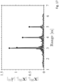
- the first scenario aims at assessing the accuracy provided by the STDREC algorithm in a single-input single-output (SISO) FMCW radar system.
- the second scenario allows us to show that the STDAEC algorithm is able to detect multiple targes contributing to the same frequency bin in a MIMO FMCW radar system and to generate accurate estimates of their spatial coordinates.
- the third scenario aims at showing that the accuracy of the 2D and 3D images generated by the two proposed embodiments is substantially better than that provided by standard algorithms based on the computation of multidimensional FFTs; in this case, both FMCW and SFCW radar systems are considered.
- RMSE root mean square error
- Scenario #1 The first scenario is characterized by four point targets having different radar cross sections (RCSs). The exact range and RCS of each of these targets are listed in Table 1.
- RCSs radar cross sections
- An FMCW radar system equipped with a single transmit and a single receive antenna is considered in this case and the STDREC algorithm is employed for range estimation only.
- Scenario #2 The second scenario is characterized by four point targets having the same range and placed at the vertices of a rectangle; moreover, the line connecting the centre of the radar with that of the rectangle is orthogonal to the rectangle itself.
- a 3D representation of the targets together with the estimated position and the associated RCS is shown in Figure 18 .
- the coordinates and the RCS of each of these targets are listed in Table 2.
- the amplitudes of the elements of the vector X VULA 0 0 see eq. (2.33)), the amplitudes of the elements of the vector X 0 VF 0 generated by vertical folding (see eq.
- Scenario #3 The third scenario is characterized by nine point targets grouped in three clusters, each made of three points having similar ranges.
- the target coordinates, the RCS and their estimates for a FMCW (SFCW) radar system are listed in Table 3 (Table 5) for the first embodiment and in Table 4 (Table 6) for the second embodiment.
- N 0 256 (see eq.
- the threshold T STDAEC is equal to the 3% of the initial energy ⁇ X (0) [ l ] ⁇ 2 measured in the considered frequency bin (see eq. (2.30)).
- the 3D image generated by both radar systems through the first embodiment is shown in Figure 20 .
- the STDAEC algorithm allows to detect all the targets, and to estimate their horizontal and vertical spatial frequencies.
- the RMSE and the peak error achieved by both systems are listed in Table 7.
Landscapes
- Engineering & Computer Science (AREA)
- Radar, Positioning & Navigation (AREA)
- Remote Sensing (AREA)
- Computer Networks & Wireless Communication (AREA)
- Physics & Mathematics (AREA)
- General Physics & Mathematics (AREA)
- Signal Processing (AREA)
- Radar Systems Or Details Thereof (AREA)
- Variable-Direction Aerials And Aerial Arrays (AREA)
Claims (16)
- Verfahren zur Erkennung von Zielen mittels eines MIMO-FMCW-Radars, das mit einer Vielzahl von Sendeantennen (TX) und Empfangsantennen (RX) ausgestattet ist, wobei jedes Paar aus TX- und RX-Antennen durch die entsprechende virtuelle Antenne ersetzt wird; wobei die Empfangsseite des MIMO-FMCW-Radars dazu eingerichtet ist, reelle oder komplexe herunterkonvertierte Signale als Reaktion auf ein Ausbreitungsszenario mit einer Vielzahl von Punktzielen zu erzeugen; wobei das Verfahren Folgendes umfasst:(Schritt 1: FFT-Verarbeitung) Schätzung des Spektrums (
X 0 (v) ) des Signals und seiner ersten NFFT - 1 Ableitungen ({X k (v); k = 1,..., NFFT - 1}) mit NFFT = 3, wenn das Signal reell ist, und NFFT = 4, wenn das Signal komplex ist, für jede der virtuellen Antennen durch FFT-Berechnung mit einem Oversampling-Faktor (M),(Schritt 2: RVA-Auswahl) Erfassung einer Teilmenge einer Anzahl (NA ) von virtuellen Antennenspektren und der zugehörigen Ableitungen,rekursive Ausführung von:(Schritt 3: STDREC-S1) Berechnung einer Schätzung der Parameter des dominantesten Punktziels, einschließlich Phase (φ), Amplitude (a) und Frequenz (f) für jede virtuelle Antenne der genannten Teilmenge auf Basis des Spektrums und dessen Ableitungen mittels NFFT - 1 FFTs für jede dieser virtuellen Antennen,(Schritt 4: STDREC-S2) Unterdrückung des dominantesten Punktziels und Berechnung eines Restspektrums und seiner ersten NFFT - 1 Ableitungen,(Schritt 5: STDREC-S3) Berechnung der Energie des Restspektrums und Rücckehr zu Schritt 3, bis die Energie einen vorgegebenen Schwellwert (Tstdrec ) übersteigt, andernfalls:
(Schritt 6) Berechnung einer durchschnittlichen Energie und Fusion der Entfernungsinformationen der durch die virtuellen Antennen erkannten Punktziele, um diese gemäß der durchschnittlichen Energie in absteigender Reihenfolge aufzulisten. - Verfahren nach Anspruch 1, wobei die Empfangsseite des Radars ein herunterkonvertiertes reelles Signal erzeugt, wobei die Berechnung in Schritt 3 Folgendes umfasst:
(Schritt 3.1.0) Darstellung einer normierten Frequenz des Ziels

X 0,α̃ (v) bestimmt wird, das dem Betrag nach größten Wert in einer ersten Hälfte plus eins der Elemente desselben VektorsX 0 (v) entspricht, und wobei die Restfrequenz durch ein iteratives Verfahren zusammen mit der entsprechenden komplexen Zielamplitude
- Verfahren nach Anspruch 1, wobei die Empfangsseite des Radars ein herunterkonvertiertes komplexes Signal erzeugt, wobei die Berechnung in Schritt 3 Folgendes umfasst:
(Schritt 3.3.0) Darstellung einer normierten Frequenz des Ziels

X 0,α̃ (v) bestimmt wird, das dem Betrag nach größten Wert desselben VektorsX 0 (v) entspricht, und wobei die Restfrequenz durch ein iteratives Verfahren zusammen mit der entsprechenden komplexen Zielamplitude
- Verfahren nach Anspruch 1, wobei die Unterdrückung (Schritt 4) die Berechnung und Subtraktion des Beitrags des dominantesten Punktziels zum Spektrum (
X 0 (v) ) und zu den entsprechenden Ableitungen umfasst, um einen Rest des Spektrums und der entsprechenden Ableitungen zu berechnen. - Verfahren nach Anspruch 1, wobei die Fusion (Schritt 6) Folgendes umfasst:
(Schritt 6.1) Fusion der Informationen, bereitgestellt durch eine Anzahl (NA ) von Teilmengen, die alle diskretisierten Entfernungen, sogenannte Frequenz-Bins, der Vielzahl von auf jeder virtuellen Antenne erkannten Ziele sammeln, zur Erzeugung der Gesamtmenge derjenigen Frequenz-Bins, die in mindestens einer dieser Teilmengen erscheinen. - Verfahren nach einem der vorhergehenden Ansprüche, das des Weiteren folgende Schritte umfasst:(Schritt 7) Erfassung des Spektrums (
X 0 (v) ) des Signals und seiner ersten NFFT - 1 Ableitungen ({X k (v); k = 1,..., NFFT - 1}) mit NFFT = 3, wenn das Signal reell ist, und NFFT = 4, wenn das Signal komplex ist, für jede der virtuellen Antennen,(Schritt 8) Erfassung einer Liste einer vorbestimmten Anzahl diskretisierter Entfernungen, sogenannter Frequenz-Bins, der erkannten Punktziele,(Schritt 9) Auswahl einer Referenzantenne, eines Referenz-Horizontal-Uniform-Linear-Arrays, genannt Referenz-HULA,(Schritt 10 [STDAEC]) sequentielle Ausführung für jeden dieser Frequenz-Bins; wobei diese Ausführung Folgendes umfasst:
(Schritt 10.1 [STDAEC-S1]) Schätzung der horizontalen räumlichen Frequenz und der komplexen Amplitude des dominantesten Punktziels; wobei diese Schätzung Folgendes umfasst:(Schritt 10.1.4 [STDAE-S4]) Berechnung des Spektrums (s HULA,0 ) und seiner ersten drei Ableitungen ({s HULA,k ; k = 1,2,3}) der Sequenz, die die Proben des Spektrums (X 0 ) enthält, bezogen auf die Referenz-HULA im betrachteten Frequenz-Bin; wobei diese Berechnungen durch FFT mit einem zweiten Oversampling-Faktor (M ) durchgeführt werden,(Schritt 10.1.5 [STDAE-S4]) Schätzung der genannten horizontalen räumlichen Frequenz,(Schritt 10.1.6 [STDAE-S5]) Überprüfung, ob die Kombination der Spektren, die mit der Referenz-HULA verbunden sind und nach Kompensation ihrer Phasendifferenzen auf Grundlage der geschätzten horizontalen Frequenz, einen Amplitudenpeak im Betrag des resultierenden Spektrums erzeugt, genannt Gesamt-Faltungsspektrum; und wenn die Überprüfung positiv ist, Ausführung folgender Schritte:(Schritt 10.1.7) Verfeinerung der Entfernung und komplexen Amplitude des dominantesten Punktziels;(Schritt 10.2 [STDAEC-S2]) Unterdrückung des dominantesten Punktziels,(Schritt 10.3 [STDAEC-S3]) Berechnung einer Restenergie im betrachteten Frequenz-Bin und Vergleich mit einem vorgegebenen Schwellwert (Tstdaec ), und Überprüfung, ob die Restenergie diesen Schwellwert übersteigt, und falls ja, Rückkehr zur Berechnung des Spektrums (Schritt 10.1.4) und Übergang zur Berechnung der räumlichen Koordinaten (Schritt 11),andernfalls, im negativen Fall der Überprüfung nach Schritt 10.1.6, Ausführung folgender Schritte:
(Schritt 10.4) Aktualisierung der erfassten Liste der Frequenz-Bins und Rücckehr zu Schritt 10 für einen weiteren Frequenz-Bin oder Beendigung, wenn alle Frequenz-Bins untersucht wurden, wobei die sequentielle Ausführung (Schritt 10) endet, wenn alle Frequenz-Bins analysiert wurden, anschließend:(Schritt 11) Berechnung der räumlichen Koordinaten aller Punktziele, die zu allen Frequenz-Bins gehören, auf Basis der genannten räumlichen Frequenz und komplexen Amplitude sowie Erzeugung eines Gesamtbildes des Ausbreitungsszenarios. - Verfahren nach Anspruch 6, wobei die virtuellen Antennen ein virtuelles Array bilden, das aus einem oder mehreren horizontalen uniformen linearen Arrays (HULAs) und einem oder mehreren vertikalen uniformen linearen Arrays (VULAs) besteht; wobei das Verfahren folgende Schritte umfasst:(Schritt 7) Erfassung des Spektrums (
X 0 (v) ) des Signals und seiner ersten NFFT - 1 Ableitungen ({X k (v); k = 1,..., NFFT - 1}) mit NFFT = 3, wenn das Signal reell ist, und NFFT = 4, wenn das Signal komplex ist, für jede der virtuellen Antennen,(Schritt 8) Erfassung einer Liste einer vorbestimmten Anzahl diskretisierter Entfernungen, sogenannte Frequenz-Bins, der erkannten Punktziele,(Schritt 9) Auswahl einer Referenzantenne, zusätzlich eines Referenz-Vertikal-Uniform-Linear-Arrays, genannt Referenz-VULA, eines Referenz-Horizontal-Uniform-Linear-Arrays, genannt Referenz-HULA, sowie mindestens einer Teilmenge von HULAs, die sich von dem Referenz-HULA unterscheidet,(Schritt 10 [STDAEC]) sequentielle Ausführung für jeden der genannten Frequenz-Bins; wobei diese Ausführung Folgendes umfasst:
(Schritt 10.1 [STDAEC-S1]) Schätzung der horizontalen räumlichen Frequenz und der komplexen Amplitude des dominantesten Punktziels sowie zusätzlich der vertikalen räumlichen Frequenz; wobei diese Schätzung Folgendes umfasst:(Schritt 10.1.1 [STDAE-S1]) Berechnung des Spektrums (s VULA,0 ) der Sequenz, die die Proben des Spektrums (X 0 ) enthält, bezogen auf das Referenz-VULA im betrachteten Frequenz-Bin, und dessen erste drei Ableitungen ({s VULA,k ; k = 1,2,3}) mittels FFT mit einem ersten Oversampling-Faktor (M ),(Schritt 10.1.2 [STDAE-S2]) Schätzung der vertikalen räumlichen Frequenz,(Schritt 10.1.3 [STDAE-S3]) Kombination der Spektren, die mit dem Referenz-HULA und der Teilmenge der HULAs verbunden sind, nach Kompensation der Phasendifferenzen zwischen Referenz-HULA und Teilmenge unter Verwendung der geschätzten vertikalen räumlichen Frequenz (Fv ); wobei diese Überlagerung, genannt vertikale Faltung, ein vertikal gefaltetes Spektrum erzeugt,(Schritt 10.1.4 [STDAE-S4]) Berechnung des Spektrums (s HULA,0 ) und seiner ersten drei Ableitungen ({s HULA,k ; k = 1,2,3}) der Sequenz, die die Proben des Spektrums (X 0 ) enthält, bezogen auf das Referenz-HULA im betrachteten Frequenz-Bin; wobei dieses Spektrum auf das vertikal gefaltete Spektrum bezogen ist und die Berechnungen mittels FFT mit einem zweiten Oversampling-Faktor (M ) durchgeführt werden,(Schritt 10.1.5 [STDAE-S4]) Schätzung der horizontalen räumlichen Frequenz,(Schritt 10.1.6 [STDAE-S5]) Überprüfung, ob die Kombination der Spektren, die mit den virtuellen Antennen der Teilmenge der HULAs verbunden sind und nach Phasenkorrektur gemäß der geschätzten horizontalen und vertikalen Frequenz einen Amplitudenpeak im Betrag des resultierenden Spektrums erzeugt, genannt Gesamt-Faltungsspektrum; und wenn die Überprüfung positiv ist, Ausführung folgender Schritte:(Schritt 10.1.7) Verfeinerung der Entfernung und komplexen Amplitude des dominantesten Punktziels;(Schritt 10.2 [STDAEC-S2]) Unterdrückung des dominantesten Punktziels,(Schritt 10.3 [STDAEC-S3]) Berechnung einer Restenergie im betrachteten Frequenz-Bin und Vergleich mit einem vorgegebenen Schwellwert (Tstdaec ), und Überprüfung, ob die Restenergie diesen Schwellwert übersteigt, und falls ja, Rückkehr zur Berechnung des Spektrums (Schritt 10.1.1), andernfalls Übergang zur Berechnung der räumlichen Koordinaten (Schritt 11),andernfalls, im negativen Fall der Überprüfung nach Schritt 10.1.6, Ausführung folgender Schritte:(Schritt 10.4) Aktualisierung der erfassten Liste der Frequenz-Bins und Rücckehr zu Schritt 10 für einen weiteren Frequenz-Bin oder Beendigung, wenn alle Frequenz-Bins untersucht wurden,wobei die sequentielle Ausführung in Schritt 10 endet, wenn alle Frequenz-Bins analysiert wurden, anschließend:
(Schritt 11) Berechnung der räumlichen Koordinaten aller Punktziele, die zu allen Frequenz-Bins gehören, auf Basis der räumlichen Frequenzen und der komplexen Amplitude sowie Erzeugung eines Gesamtbildes des Ausbreitungsszenarios. - Verfahren zur Erkennung von Zielen mittels eines MIMO-SFCW-Radars, das mit einer Vielzahl von Sendeantennen (TX) und Empfangsantennen (RX) ausgestattet ist, wobei jedes Paar aus TX- und RX-Antennen durch die entsprechende virtuelle Antenne ersetzt wird; wobei die Empfangsseite des MIMO-SFCW-Radars dazu eingerichtet ist, komplexe herunterkonvertierte Signale als Reaktion auf ein Ausbreitungsszenario mit einer Vielzahl von Punktzielen zu erzeugen; wobei das Verfahren folgende Schritte umfasst:(Schritt 1: IFFT-Verarbeitung) Schätzung der Impulsantwort (
X 0 (v) ), die den Übertragungskanal der entsprechenden virtuellen Antenne charakterisiert, und deren erster NFFT - 1 Ableitungen ({X k (v); k = 1,..., NFFT - 1}) mit NFFT = 4, für jede der virtuellen Antennen mittels IFFT-Berechnung mit einem Oversampling-Faktor (M),(Schritt 2: RVA-Auswahl) Erfassung einer Teilmenge einer Anzahl NA von Impulsantworten virtueller Antennen und der zugehörigen Ableitungen,rekursive Ausführung von:(Schritt 3: STDREC-S1) Berechnung einer Schätzung der Parameter des dominantesten Punktziels, einschließlich Phase (ψ), Amplitude (α) und Verzögerung (τ) für jede virtuelle Antenne der genannten Teilmenge auf Basis der Impulsantwort und deren Ableitungen durch NFFT - 1 IFFTs für jede dieser virtuellen Antennen,(Schritt 4: STDREC-S2) Unterdrückung des dominantesten Punktziels und Berechnung einer Restimpulsantwort und deren erster NFFT - 1 Ableitungen,(Schritt 5: STDREC-S3) Berechnung der Energie der Restimpulsantwort und Rückkehr zu Schritt 3, solange die Energie einen vorgegebenen Schwellwert (Tstdrec ) übersteigt, andernfalls:
(Schritt 6) Berechnung einer durchschnittlichen Energie und Fusion der Entfernungsinformationen der durch die virtuellen Antennen erkannten Punktziele, um diese gemäß der durchschnittlichen Energie in absteigender Reihenfolge aufzulisten. - Verfahren nach Anspruch 8, wobei die Berechnung (Schritt 3) Folgendes umfasst:
(Schritt 3.5.0) Darstellung einer normierten Verzögerung eines Ziels
X 0,α̃ (v) bestimmt wird, das dem Betrag nach größten Wert desselben VektorsX 0 (v) entspricht, und wobei der Restanteil durch ein iteratives Verfahren zusammen mit der entsprechenden komplexen Zielamplitude
- Verfahren nach Anspruch 8, wobei die Unterdrückung (Schritt 4) die Berechnung und Subtraktion des Beitrags des dominantesten Punktziels zur Impulsantwort (
X 0 (v) ) und zu den entsprechenden Ableitungen umfasst, um einen Rest der Impulsantwort und der entsprechenden Ableitungen zu berechnen. - Verfahren nach Anspruch 8, wobei die Fusion in Schritt 6 Folgendes umfasst:
(Schritt 6.1) Fusion der Informationen, bereitgestellt durch eine Anzahl (NA ) von Teilmengen, die alle diskretisierten Entfernungen, sogenannte Verzögerungs-Bins, der Vielzahl von auf jeder virtuellen Antenne erkannten Ziele sammeln, zur Erzeugung der Gesamtmenge derjenigen Verzögerungs-Bins, die in mindestens einer dieser Teilmengen erscheinen. - Verfahren nach einem der vorhergehenden Ansprüche 8 bis 11, das des Weiteren folgende Schritte umfasst:(Schritt 7) Erfassung der Impulsantwort (
X 0 (v) ), die den Übertragungskanal der entsprechenden virtuellen Antenne charakterisiert, und deren ersten NFFT - 1 Ableitungen ({X k (v); k = 1,..., NFFT - 1}) mit NFFT = 4, für jede der virtuellen Antennen,(Schritt 8) Erfassung einer Liste einer vorbestimmten Anzahl diskretisierter Entfernungen, sogenannte Verzögerungs-Bins, der erkannten Punktziele,(Schritt 9) Auswahl einer Referenzantenne, eines Referenz-Horizontal-Uniform-Linear-Arrays, genannt Referenz-HULA,(Schritt 10 [STDAEC]) sequentielle Ausführung für jeden der genannten Verzögerungs-Bins; wobei diese Ausführung Folgendes umfasst:
(Schritt 10.1 [STDAEC-S1]) Schätzung der horizontalen räumlichen Verzögerung und der komplexen Amplitude des dominantesten Punktziels; wobei diese Schätzung Folgendes umfasst:(Schritt 10.1.4 [STDAE-S4]) Berechnung des Spektrums Spektrums (s HULA,0 ) und seiner ersten drei Ableitungen ({s HULA,k ; k = 1,2,3}) der Sequenz, die die Proben der Impulsantwort (X 0 ) enthält, bezogen auf das Referenz-HULA im betrachteten Verzögerungs-Bin; wobei diese Berechnungen durch IFFT mit einem Oversampling-Faktor (M ) durchgeführt werden,(Schritt 10.1.5 [STDAE-S4]) Schätzung der genannten horizontalen räumlichen Verzögerung,(Schritt 10.1.6 [STDAE-S5]) Überprüfung, ob die Kombination der Impulsantworten, die mit den virtuellen Antennen des Referenz-HULA verbunden sind, nach Kompensation ihrer Phasendifferenzen auf Grundlage der geschätzten horizontalen Verzögerung, einen Amplitudenpeak im Betrag der resultierenden Impulsantwort erzeugt, genannt Gesamt-Faltungsimpulsantwort; und wenn die Überprüfung positiv ist, Ausführung folgender Schritte:(Schritt 10.1.7) Verfeinerung der Entfernung und komplexen Amplitude des dominantesten Punktziels;(Schritt 10.2 [STDAEC-S2]) Unterdrückung des dominantesten Punktziels,(Schritt 10.3 [STDAEC-S3]) Berechnung einer Restenergie im betrachteten Verzögerungs-Bin und Vergleich mit einem vorgegebenen Schwellwert (Tstdaec ), und Überprüfung, ob die Restenergie diesen Schwellwert übersteigt, und falls ja, Rückkehr zur Berechnung des Spektrums (Schritt 10.1.4), andernfalls Übergang zur Berechnung der räumlichen Koordinaten (Schritt 11),andernfalls, im negativen Fall der Überprüfung nach Schritt 10.1.6, Ausführung folgender Schritte:(Schritt 10.4) Aktualisierung der erfassten Liste der Verzögerungs-Bins und Rückkehr zu Schritt 10 für einen weiteren Verzögerungs-Bin oder Beendigung, wenn alle Verzögerungs-Bins untersucht wurden,wobei die Ausführung in Schritt 10 endet, wenn alle Verzögerungs-Bins analysiert wurden, anschließend:
(Schritt 11) Berechnung der räumlichen Koordinaten aller Punktziele, die zu allen Verzögerungs-Bins gehören, auf Basis der räumlichen Verzögerungen und der komplexen Amplitude sowie Erzeugung eines Gesamtbildes des Ausbreitungsszenarios. - Verfahren nach Anspruch 12, wobei die virtuellen Antennen ein virtuelles Array bilden, das aus einem oder mehreren horizontalen uniformen linearen Arrays (HULAs) und einem oder mehreren vertikalen uniformen linearen Arrays (VULAs) besteht; wobei das Verfahren folgende Schritte umfasst:(Schritt 7) Erfassung der Impulsantwort (
X 0 (v) ), die den Übertragungskanal der entsprechenden virtuellen Antenne charakterisiert, und deren ersten NFFT - 1 Ableitungen ({X k (v); k = 1,..., NFFT - 1}) mit NFFT = 4, für jede der virtuellen Antennen,(Schritt 8) Erfassung einer Liste einer vorbestimmten Anzahl diskretisierter Entfernungen, sogenannte Verzögerungs-Bins, der erkannten Punktziele,(Schritt 9) Auswahl einer Referenzantenne, eines Referenz-Vertikal-Uniform-Linear-Arrays, genannt Referenz-VULA, eines Referenz-Horizontal-Uniform-Linear-Arrays, genannt Referenz-HULA, sowie mindestens einer Teilmenge von HULAs, die sich von dem Referenz-HULA unterscheidet,(Schritt 10 [STDAEC]) sequenzielle Ausführung für jeden der genannten Verzögerungs-Bins; wobei diese Ausführung Folgendes umfasst:
(Schritt 10.1 [STDAEC-S1]) Schätzung der horizontalen räumlichen Verzögerung und der komplexen Amplitude des dominantesten Punktziels sowie Schätzung der vertikalen räumlichen Verzögerung; wobei diese Schätzung Folgendes umfasst:(Schritt 10.1.1 [STDAE-S1]) Berechnung des Spektrums (s VULA,0 ) der Sequenz, die die Proben der Impulsantwort (X 0 ) enthält, bezogen auf das Referenz-VULA im betrachteten Verzögerungs-Bin, und deren erster drei Ableitungen ({s VULA,k ; k = 1,2,3}) mittels IFFT mit einem Oversampling-Faktor (M ),(Schritt 10.1.2 [STDAE-S2]) Schätzung der vertikalen räumlichen Verzögerung,(Schritt 10.1.3 [STDAE-S3]) Kombination der Spektren, die mit dem Referenz-HULA und der Teilmenge der HULAs verbunden sind, nach Kompensation der Phasendifferenzen zwischen Referenz-HULA und der Teilmenge unter Verwendung der geschätzten vertikalen räumlichen Verzögerung (Tv ); wobei diese Überlagerung, genannt vertikale Faltung, eine vertikal gefaltete Impulsantwort erzeugt,(Schritt 10.1.4 [STDAE-S4]) Berechnung des Spektrums (s HULA,0 ) und seiner ersten drei Ableitungen ({s HULA,k ; k = 1,2,3}) der Sequenz, die die Proben der Impulsantwort (X 0 ) enthält, bezogen auf das Referenz-HULA im betrachteten Verzögerungs-Bin; wobei dieses Spektrum auf die vertikal gefaltete Impulsantwort bezogen ist und die Berechnungen durch IFFT mit einem Oversampling-Faktor (M ) erfolgen,(Schritt 10.1.5 [STDAE-S4]) Schätzung der horizontalen räumlichen Verzögerung,(Schritt 10.1.6 [STDAE-S5]) Überprüfung, ob die Kombination der Impulsantworten, die mit den virtuellen Antennen der Referenz-HULA verbunden sind, nach Phasenkorrektur gemäß der geschätzten horizontalen und vertikalen Verzögerung, einen Amplitudenpeak im Betrag der resultierenden Impulsantwort erzeugt, genannt Gesamt-Faltungsimpulsantwort; und wenn die Überprüfung positiv ist, Ausführung folgender Schritte:(Schritt 10.1.7) Verfeinerung der Entfernung und komplexen Amplitude des dominantesten Punktziels;(Schritt 10.2 [STDAEC-S2]) Unterdrückung des dominantesten Punktziels,(Schritt 10.3 [STDAEC-S3]) Berechnung einer Restenergie im betrachteten Verzögerungs-Bin und Vergleich mit einem vorgegebenen Schwellwert (Tstdaec ), und Überprüfung, ob die Restenergie diesen Schwellwert übersteigt, und falls ja, Rückkehr zur Berechnung des Spektrums (Schritt 10.1.1 oder 10.1.4), andernfalls Übergang zur Berechnung der räumlichen Koordinaten (Schritt 11),andernfalls, im negativen Fall der Überprüfung nach Schritt 10.1.6, Ausführung folgender Schritte:(Schritt 10.4) Aktualisierung der erfassten Liste der Verzögerungs-Bins und Rückkehr zu Schritt 10 für einen weiteren Verzögerungs-Bin oder Beendigung, wenn alle Verzögerungs-Bins untersucht wurden,wobei die Ausführung in Schritt 10 endet, wenn alle Verzögerungs-Bins analysiert wurden, anschließend:
(Schritt 11) Berechnung der räumlichen Koordinaten aller Punktziele, die zu allen Verzögerungs-Bins gehören, auf Basis der räumlichen Verzögerungen und der komplexen Amplitude sowie Erzeugung eines Gesamtbildes des Ausbreitungsszenarios. - Verfahren nach Anspruch 6 bis 7 oder 12 bis 13, das des Weiteren die Kompensation der Amplitudenverzerrung infolge der nicht-uniformen Antwort des Antennenarrays für jede der virtuellen Antennen auf Basis der verfeinerten komplexen Amplitude (Schritt 10.1.7) und der geschätzten räumlichen Frequenzen umfasst, wobei diese Kompensation Folgendes umfasst:(Schritt 10.1.8) Nutzung eines tiefen neuronalen Netzwerks, das zur Lösung eines Regressionsproblems mittels überwachtem Lernverfahren entworfen wurde, wobei das Training des Netzwerks auf einem Datensatz basiert, der die Amplituden einer Anzahl von Punktzielen umfasst,wobei die Kompensation der komplexen Amplitude durch Multiplikation der verfeinerten Schätzung der komplexen Amplitude (Schritt 10.1.7) mit der geschätzten Amplitudenverzerrung für jede der virtuellen Antennen erfolgt.
- MIMO-FMCW-Radarsystem mit:einem MIMO-FMCW-Radar, ausgestattet mit einer Vielzahl von Sendeantennen (TX) und Empfangsantennen (RX), die dazu eingerichtet sind, reelle oder komplexe Signale als Reaktion auf ein Ausbreitungsszenario mit einer Vielzahl von Punktzielen zu erzeugen, undeiner Recheneinheit, die dazu eingerichtet ist, die von den Sende- und Empfangsantennen erzeugten Signale zu empfangen und jeweils ein Paar aus Sende- und Empfangsantenne durch ein äquivalentes Modell zu ersetzen, das virtuelle Antennen definiert, und alle Schritte eines der vorhergehenden Ansprüche 1 bis 7 und 14 auszuführen.
- MIMO-SFCW-Radarsystem mit:einem MIMO-SFCW-Radar, ausgestattet mit einer Vielzahl von Sendeantennen (TX) und Empfangsantennen (RX), die dazu eingerichtet sind, komplexe Signale als Reaktion auf ein Ausbreitungsszenario mit einer Vielzahl von Punktzielen zu erzeugen, undeiner Recheneinheit, die dazu eingerichtet ist, die von den Sende- und Empfangsantennen erzeugten Signale zu empfangen und jeweils ein Paar aus Sende- und Empfangsantenne durch ein äquivalentes Modell zu ersetzen, das virtuelle Antennen definiert, und alle Schritte eines der vorhergehenden Ansprüche 8 bis 14 auszuführen.
Applications Claiming Priority (3)
| Application Number | Priority Date | Filing Date | Title |
|---|---|---|---|
| IT102021000011156A IT202100011156A1 (it) | 2021-05-03 | 2021-05-03 | Metodo per l'imaging bidimensionale e tridimensionale basato su radar a ingressi multipli e uscite multiple co-locati |
| IT202100011243 | 2021-05-03 | ||
| PCT/EP2022/061874 WO2022233887A1 (en) | 2021-05-03 | 2022-05-03 | Method for two-dimensional and three-dimensional imaging based on colocated multiple-input multiple-output radars |
Publications (2)
| Publication Number | Publication Date |
|---|---|
| EP4334740A1 EP4334740A1 (de) | 2024-03-13 |
| EP4334740B1 true EP4334740B1 (de) | 2025-06-04 |
Family
ID=81849297
Family Applications (3)
| Application Number | Title | Priority Date | Filing Date |
|---|---|---|---|
| EP22726140.1A Active EP4334740B1 (de) | 2021-05-03 | 2022-05-03 | Verfahren zur zweidimensionalen und dreidimensionalen bildgebung auf der basis von benachbarten radaren mit mehreren eingängen und mehreren ausgängen |
| EP22726142.7A Pending EP4334742A1 (de) | 2021-05-03 | 2022-05-03 | Verfahren zur rechnerschätzung eines einzeltons und deren anwendung in radarsystemen |
| EP22726141.9A Pending EP4334741A1 (de) | 2021-05-03 | 2022-05-03 | Verfahren zur zweidimensionalen und dreidimensionalen bildgebung auf basis von benachbarten radaren mit mehreren eingängen und mehreren ausgängen |
Family Applications After (2)
| Application Number | Title | Priority Date | Filing Date |
|---|---|---|---|
| EP22726142.7A Pending EP4334742A1 (de) | 2021-05-03 | 2022-05-03 | Verfahren zur rechnerschätzung eines einzeltons und deren anwendung in radarsystemen |
| EP22726141.9A Pending EP4334741A1 (de) | 2021-05-03 | 2022-05-03 | Verfahren zur zweidimensionalen und dreidimensionalen bildgebung auf basis von benachbarten radaren mit mehreren eingängen und mehreren ausgängen |
Country Status (2)
| Country | Link |
|---|---|
| EP (3) | EP4334740B1 (de) |
| WO (3) | WO2022233887A1 (de) |
Families Citing this family (6)
| Publication number | Priority date | Publication date | Assignee | Title |
|---|---|---|---|---|
| CN115987421A (zh) * | 2022-11-30 | 2023-04-18 | 杭州电子科技大学 | 无人机集群通信的抖动信道估计系统 |
| CN116047431B (zh) * | 2022-12-08 | 2026-01-13 | 中国人民解放军32181部队 | 一种高精度雷达发射机频率测试方法 |
| CN116087932A (zh) * | 2023-01-09 | 2023-05-09 | 杭州腓腓科技有限公司 | 基于可重构全息超表面的定位方法、系统、存储介质及雷达 |
| EP4418000A1 (de) * | 2023-02-17 | 2024-08-21 | IMRA Europe S.A.S. | Radardatenverarbeitung durch dnn |
| CN116735956B (zh) * | 2023-05-09 | 2025-09-02 | 中国人民解放军陆军勤务学院 | 一种抗多频干扰的实正弦信号频率高精度估计方法 |
| CN117991245B (zh) * | 2024-02-04 | 2024-07-23 | 南京畅淼科技有限责任公司 | 一种基于多通道二次dft与插值相结合的船舶方位估计方法 |
Family Cites Families (3)
| Publication number | Priority date | Publication date | Assignee | Title |
|---|---|---|---|---|
| WO2006079181A1 (en) * | 2005-01-31 | 2006-08-03 | Genesys Design Pty Ltd | Frequency estimation |
| US11346936B2 (en) * | 2018-01-16 | 2022-05-31 | Infineon Technologies Ag | System and method for vital signal sensing using a millimeter-wave radar sensor |
| DE102018119278B4 (de) * | 2018-08-08 | 2020-04-02 | Infineon Technologies Ag | Verfahren und vorrichtungen für die verarbeitung eines ofdm-radarsignals |
-
2022
- 2022-05-03 WO PCT/EP2022/061874 patent/WO2022233887A1/en not_active Ceased
- 2022-05-03 EP EP22726140.1A patent/EP4334740B1/de active Active
- 2022-05-03 WO PCT/EP2022/061876 patent/WO2022233889A1/en not_active Ceased
- 2022-05-03 EP EP22726142.7A patent/EP4334742A1/de active Pending
- 2022-05-03 WO PCT/EP2022/061875 patent/WO2022233888A1/en not_active Ceased
- 2022-05-03 EP EP22726141.9A patent/EP4334741A1/de active Pending
Also Published As
| Publication number | Publication date |
|---|---|
| EP4334741A1 (de) | 2024-03-13 |
| EP4334740A1 (de) | 2024-03-13 |
| WO2022233887A1 (en) | 2022-11-10 |
| WO2022233888A1 (en) | 2022-11-10 |
| WO2022233889A1 (en) | 2022-11-10 |
| EP4334742A1 (de) | 2024-03-13 |
Similar Documents
| Publication | Publication Date | Title |
|---|---|---|
| Ramezanpour et al. | Deep‐learning‐based beamforming for rejecting interferences | |
| Zhaocheng et al. | Sparsity-based STAP using alternating direction method with gain/phase errors | |
| Wu et al. | Space–time adaptive processing and motion parameter estimation in multistatic passive radar using sparse Bayesian learning | |
| EP4334741A1 (de) | Verfahren zur zweidimensionalen und dreidimensionalen bildgebung auf basis von benachbarten radaren mit mehreren eingängen und mehreren ausgängen | |
| Zheng et al. | Detection of ghost targets for automotive radar in the presence of multipath | |
| Wang et al. | Subspace-augmented clutter suppression technique for STAP radar | |
| US6226321B1 (en) | Multichannel parametric adaptive matched filter receiver | |
| Yang et al. | Knowledge‐aided STAP with sparse‐recovery by exploiting spatio‐temporal sparsity | |
| Zhang et al. | Maximum likelihood delay and Doppler estimation for passive sensing | |
| Zhu et al. | Low‐angle target tracking using frequency‐agile refined maximum likelihood algorithm | |
| Rosenberg et al. | Coherent detection in medium grazing angle sea‐clutter | |
| Gao et al. | Frequency diverse array MIMO radar adaptive beamforming with range‐dependent interference suppression in target localization | |
| Chung et al. | Efficient multi-user channel estimation for RIS-aided mmWave systems using shared channel subspace | |
| Huang et al. | A novel space-time interference mitigation algorithm on multichannel SAR systems | |
| Huang et al. | Aligned propagator scanning approach to DOA estimation of circular and noncircular wideband source signals | |
| CN113376607B (zh) | 机载分布式雷达小样本空时自适应处理方法 | |
| Jin et al. | Robust cyclic beamforming against cycle frequency error in Gaussian and impulsive noise environments | |
| Mirabella et al. | Deterministic signal processing techniques for OFDM-based radar sensing: An overview | |
| Li et al. | Efficient time‐varying interference suppression method for synthetic aperture radar imaging based on time‐frequency reconstruction and mask technique | |
| Rao et al. | Comparison of parametric sparse recovery methods for ISAR image formation | |
| Hassanien et al. | Robust moving target detection for distributed MIMO radar in non-homogeneous clutter | |
| Han et al. | Joint DOA and Doppler frequency estimation for MIMO radars in the presence of array model imperfections | |
| Smith et al. | Improved moving target detection in homogeneous and heterogeneous clutter with limited secondary data using unit circle roots constraints | |
| Li et al. | Robust cyclic MUSIC algorithm for finding directions in impulsive noise environment | |
| Liu et al. | Clutter-aware integrated sensing and communication: Models, methods, and future directions |
Legal Events
| Date | Code | Title | Description |
|---|---|---|---|
| STAA | Information on the status of an ep patent application or granted ep patent |
Free format text: STATUS: UNKNOWN |
|
| STAA | Information on the status of an ep patent application or granted ep patent |
Free format text: STATUS: THE INTERNATIONAL PUBLICATION HAS BEEN MADE |
|
| PUAI | Public reference made under article 153(3) epc to a published international application that has entered the european phase |
Free format text: ORIGINAL CODE: 0009012 |
|
| STAA | Information on the status of an ep patent application or granted ep patent |
Free format text: STATUS: REQUEST FOR EXAMINATION WAS MADE |
|
| 17P | Request for examination filed |
Effective date: 20231204 |
|
| AK | Designated contracting states |
Kind code of ref document: A1 Designated state(s): AL AT BE BG CH CY CZ DE DK EE ES FI FR GB GR HR HU IE IS IT LI LT LU LV MC MK MT NL NO PL PT RO RS SE SI SK SM TR |
|
| DAV | Request for validation of the european patent (deleted) | ||
| DAX | Request for extension of the european patent (deleted) | ||
| GRAP | Despatch of communication of intention to grant a patent |
Free format text: ORIGINAL CODE: EPIDOSNIGR1 |
|
| STAA | Information on the status of an ep patent application or granted ep patent |
Free format text: STATUS: GRANT OF PATENT IS INTENDED |
|
| INTG | Intention to grant announced |
Effective date: 20241213 |
|
| GRAS | Grant fee paid |
Free format text: ORIGINAL CODE: EPIDOSNIGR3 |
|
| GRAA | (expected) grant |
Free format text: ORIGINAL CODE: 0009210 |
|
| STAA | Information on the status of an ep patent application or granted ep patent |
Free format text: STATUS: THE PATENT HAS BEEN GRANTED |
|
| AK | Designated contracting states |
Kind code of ref document: B1 Designated state(s): AL AT BE BG CH CY CZ DE DK EE ES FI FR GB GR HR HU IE IS IT LI LT LU LV MC MK MT NL NO PL PT RO RS SE SI SK SM TR |
|
| REG | Reference to a national code |
Ref country code: GB Ref legal event code: FG4D |
|
| REG | Reference to a national code |
Ref country code: CH Ref legal event code: EP |
|
| REG | Reference to a national code |
Ref country code: DE Ref legal event code: R096 Ref document number: 602022015546 Country of ref document: DE |
|
| REG | Reference to a national code |
Ref country code: IE Ref legal event code: FG4D |
|
| REG | Reference to a national code |
Ref country code: NL Ref legal event code: MP Effective date: 20250604 |
|
| PG25 | Lapsed in a contracting state [announced via postgrant information from national office to epo] |
Ref country code: ES Free format text: LAPSE BECAUSE OF FAILURE TO SUBMIT A TRANSLATION OF THE DESCRIPTION OR TO PAY THE FEE WITHIN THE PRESCRIBED TIME-LIMIT Effective date: 20250604 Ref country code: FI Free format text: LAPSE BECAUSE OF FAILURE TO SUBMIT A TRANSLATION OF THE DESCRIPTION OR TO PAY THE FEE WITHIN THE PRESCRIBED TIME-LIMIT Effective date: 20250604 |
|
| REG | Reference to a national code |
Ref country code: LT Ref legal event code: MG9D |
|
| PG25 | Lapsed in a contracting state [announced via postgrant information from national office to epo] |
Ref country code: GR Free format text: LAPSE BECAUSE OF FAILURE TO SUBMIT A TRANSLATION OF THE DESCRIPTION OR TO PAY THE FEE WITHIN THE PRESCRIBED TIME-LIMIT Effective date: 20250905 Ref country code: NO Free format text: LAPSE BECAUSE OF FAILURE TO SUBMIT A TRANSLATION OF THE DESCRIPTION OR TO PAY THE FEE WITHIN THE PRESCRIBED TIME-LIMIT Effective date: 20250904 |
|
| PG25 | Lapsed in a contracting state [announced via postgrant information from national office to epo] |
Ref country code: PL Free format text: LAPSE BECAUSE OF FAILURE TO SUBMIT A TRANSLATION OF THE DESCRIPTION OR TO PAY THE FEE WITHIN THE PRESCRIBED TIME-LIMIT Effective date: 20250604 |
|
| PG25 | Lapsed in a contracting state [announced via postgrant information from national office to epo] |
Ref country code: BG Free format text: LAPSE BECAUSE OF FAILURE TO SUBMIT A TRANSLATION OF THE DESCRIPTION OR TO PAY THE FEE WITHIN THE PRESCRIBED TIME-LIMIT Effective date: 20250604 |
|
| PG25 | Lapsed in a contracting state [announced via postgrant information from national office to epo] |
Ref country code: HR Free format text: LAPSE BECAUSE OF FAILURE TO SUBMIT A TRANSLATION OF THE DESCRIPTION OR TO PAY THE FEE WITHIN THE PRESCRIBED TIME-LIMIT Effective date: 20250604 |
|
| PG25 | Lapsed in a contracting state [announced via postgrant information from national office to epo] |
Ref country code: RS Free format text: LAPSE BECAUSE OF FAILURE TO SUBMIT A TRANSLATION OF THE DESCRIPTION OR TO PAY THE FEE WITHIN THE PRESCRIBED TIME-LIMIT Effective date: 20250904 |
|
| PG25 | Lapsed in a contracting state [announced via postgrant information from national office to epo] |
Ref country code: LV Free format text: LAPSE BECAUSE OF FAILURE TO SUBMIT A TRANSLATION OF THE DESCRIPTION OR TO PAY THE FEE WITHIN THE PRESCRIBED TIME-LIMIT Effective date: 20250604 |
|
| PG25 | Lapsed in a contracting state [announced via postgrant information from national office to epo] |
Ref country code: NL Free format text: LAPSE BECAUSE OF FAILURE TO SUBMIT A TRANSLATION OF THE DESCRIPTION OR TO PAY THE FEE WITHIN THE PRESCRIBED TIME-LIMIT Effective date: 20250604 |
|
| PG25 | Lapsed in a contracting state [announced via postgrant information from national office to epo] |
Ref country code: PT Free format text: LAPSE BECAUSE OF FAILURE TO SUBMIT A TRANSLATION OF THE DESCRIPTION OR TO PAY THE FEE WITHIN THE PRESCRIBED TIME-LIMIT Effective date: 20251006 |
|
| REG | Reference to a national code |
Ref country code: AT Ref legal event code: MK05 Ref document number: 1800825 Country of ref document: AT Kind code of ref document: T Effective date: 20250604 |
|
| PG25 | Lapsed in a contracting state [announced via postgrant information from national office to epo] |
Ref country code: IS Free format text: LAPSE BECAUSE OF FAILURE TO SUBMIT A TRANSLATION OF THE DESCRIPTION OR TO PAY THE FEE WITHIN THE PRESCRIBED TIME-LIMIT Effective date: 20251004 |
|
| PG25 | Lapsed in a contracting state [announced via postgrant information from national office to epo] |
Ref country code: AT Free format text: LAPSE BECAUSE OF FAILURE TO SUBMIT A TRANSLATION OF THE DESCRIPTION OR TO PAY THE FEE WITHIN THE PRESCRIBED TIME-LIMIT Effective date: 20250604 Ref country code: SM Free format text: LAPSE BECAUSE OF FAILURE TO SUBMIT A TRANSLATION OF THE DESCRIPTION OR TO PAY THE FEE WITHIN THE PRESCRIBED TIME-LIMIT Effective date: 20250604 |
|
| PG25 | Lapsed in a contracting state [announced via postgrant information from national office to epo] |
Ref country code: CZ Free format text: LAPSE BECAUSE OF FAILURE TO SUBMIT A TRANSLATION OF THE DESCRIPTION OR TO PAY THE FEE WITHIN THE PRESCRIBED TIME-LIMIT Effective date: 20250604 |
|
| PG25 | Lapsed in a contracting state [announced via postgrant information from national office to epo] |
Ref country code: EE Free format text: LAPSE BECAUSE OF FAILURE TO SUBMIT A TRANSLATION OF THE DESCRIPTION OR TO PAY THE FEE WITHIN THE PRESCRIBED TIME-LIMIT Effective date: 20250604 |
|
| PG25 | Lapsed in a contracting state [announced via postgrant information from national office to epo] |
Ref country code: SK Free format text: LAPSE BECAUSE OF FAILURE TO SUBMIT A TRANSLATION OF THE DESCRIPTION OR TO PAY THE FEE WITHIN THE PRESCRIBED TIME-LIMIT Effective date: 20250604 |
|
| REG | Reference to a national code |
Ref country code: DE Ref legal event code: R097 Ref document number: 602022015546 Country of ref document: DE |
|
| PLBE | No opposition filed within time limit |
Free format text: ORIGINAL CODE: 0009261 |
|
| STAA | Information on the status of an ep patent application or granted ep patent |
Free format text: STATUS: NO OPPOSITION FILED WITHIN TIME LIMIT |
|
| PG25 | Lapsed in a contracting state [announced via postgrant information from national office to epo] |
Ref country code: DK Free format text: LAPSE BECAUSE OF FAILURE TO SUBMIT A TRANSLATION OF THE DESCRIPTION OR TO PAY THE FEE WITHIN THE PRESCRIBED TIME-LIMIT Effective date: 20250604 |
|
| REG | Reference to a national code |
Ref country code: CH Ref legal event code: L10 Free format text: ST27 STATUS EVENT CODE: U-0-0-L10-L00 (AS PROVIDED BY THE NATIONAL OFFICE) Effective date: 20260416 |
|
| 26N | No opposition filed |
Effective date: 20260305 |