EP4296901A1 - Abbildung von neuronalen netzen auf hardware - Google Patents
Abbildung von neuronalen netzen auf hardware Download PDFInfo
- Publication number
- EP4296901A1 EP4296901A1 EP23180122.6A EP23180122A EP4296901A1 EP 4296901 A1 EP4296901 A1 EP 4296901A1 EP 23180122 A EP23180122 A EP 23180122A EP 4296901 A1 EP4296901 A1 EP 4296901A1
- Authority
- EP
- European Patent Office
- Prior art keywords
- depth
- hardware
- coefficients
- size
- group
- Prior art date
- Legal status (The legal status is an assumption and is not a legal conclusion. Google has not performed a legal analysis and makes no representation as to the accuracy of the status listed.)
- Pending
Links
Images







Classifications
-
- G—PHYSICS
- G06—COMPUTING OR CALCULATING; COUNTING
- G06N—COMPUTING ARRANGEMENTS BASED ON SPECIFIC COMPUTATIONAL MODELS
- G06N3/00—Computing arrangements based on biological models
- G06N3/02—Neural networks
- G06N3/04—Architecture, e.g. interconnection topology
-
- G—PHYSICS
- G06—COMPUTING OR CALCULATING; COUNTING
- G06N—COMPUTING ARRANGEMENTS BASED ON SPECIFIC COMPUTATIONAL MODELS
- G06N3/00—Computing arrangements based on biological models
- G06N3/02—Neural networks
- G06N3/06—Physical realisation, i.e. hardware implementation of neural networks, neurons or parts of neurons
- G06N3/063—Physical realisation, i.e. hardware implementation of neural networks, neurons or parts of neurons using electronic means
-
- G—PHYSICS
- G06—COMPUTING OR CALCULATING; COUNTING
- G06N—COMPUTING ARRANGEMENTS BASED ON SPECIFIC COMPUTATIONAL MODELS
- G06N3/00—Computing arrangements based on biological models
- G06N3/02—Neural networks
- G06N3/04—Architecture, e.g. interconnection topology
- G06N3/0495—Quantised networks; Sparse networks; Compressed networks
-
- G—PHYSICS
- G06—COMPUTING OR CALCULATING; COUNTING
- G06N—COMPUTING ARRANGEMENTS BASED ON SPECIFIC COMPUTATIONAL MODELS
- G06N3/00—Computing arrangements based on biological models
- G06N3/02—Neural networks
- G06N3/08—Learning methods
- G06N3/082—Learning methods modifying the architecture, e.g. adding, deleting or silencing nodes or connections
-
- G—PHYSICS
- G06—COMPUTING OR CALCULATING; COUNTING
- G06N—COMPUTING ARRANGEMENTS BASED ON SPECIFIC COMPUTATIONAL MODELS
- G06N3/00—Computing arrangements based on biological models
- G06N3/02—Neural networks
- G06N3/04—Architecture, e.g. interconnection topology
- G06N3/0464—Convolutional networks [CNN, ConvNet]
-
- G—PHYSICS
- G06—COMPUTING OR CALCULATING; COUNTING
- G06N—COMPUTING ARRANGEMENTS BASED ON SPECIFIC COMPUTATIONAL MODELS
- G06N5/00—Computing arrangements using knowledge-based models
- G06N5/01—Dynamic search techniques; Heuristics; Dynamic trees; Branch-and-bound
Definitions
- Determining a starting value of a current depth within the binary tree may comprise setting the starting value of the current depth to a depth of one and wherein updating the current depth comprises increasing the current depth.
- Updating the current depth may comprise decreasing the current depth and wherein the termination criteria comprise: the compressed group size exceeds the hardware size constraint; and the current depth is less than the starting depth minus one.
- a second aspect provides a method of implementing a neural network using a hardware accelerator comprising fixed function circuitry, the method comprising using a binary tree to assess how to split a layer of the neural network into a plurality of hardware passes, each hardware pass reading a subset of the coefficients of the layer from external memory and wherein the coefficients are stored in compressed form in the memory and each node in the binary tree corresponding to a different subset of the coefficients, wherein using the binary tree comprises: (i) determining a starting value of a current depth within the binary tree; (ii) arranging the set of coefficients into groups, each group corresponding to a node at the current depth; (iii) calculating a compressed size of at least one group of coefficients at the current depth; (iv) determining whether termination criteria are satisfied, at least one of the termination criteria being based on a comparison between the calculated compressed size and a hardware size constraint; (v) in response to determining that the termination criteria are not satisfied, updating the current depth and repeating steps (ii
- the method of implementing a neural network may further comprise: executing the layer of the neural network, using the fixed function circuitry, according to the data defining each of the plurality of hardware passes.
- a third aspect provides a computing device comprising a processor and a memory, wherein the memory is arranged to store computer readable code configured to cause any of the methods described herein to be performed when the code is executed by the processor
- the array of weights for a layer in a NN may be stored in compressed form in order to reduce the amount of storage required and the bandwidth used to read the weights from memory.
- the weights may also be referred to as 'coefficients' and the two terms are used interchangeably herein.
- the coefficients are read from memory and stored in a buffer (which may be referred to as the coefficient buffer) within the NN hardware (e.g. within a NN accelerator, NNA) before being decompressed and fed into the hardware elements (which may be referred to as 'processing elements') that apply the coefficients to the input data (e.g. into the convolution engines within the NNA).
- the coefficient buffer is not large enough to store all the coefficients for a NN layer (e.g. because of the large sizes of the arrays and constraints on the space and power available for the buffer) and/or there is insufficient bandwidth available between the memory and the NNA to read all the coefficients from a NN layer into the buffer in the available time (i.e. there is a limit on the amount of data that can be loaded in each clock cycle).
- the loading of the coefficients for a layer is divided into a plurality of operations, referred to as 'passes' or 'hardware passes', where each pass involves reading a subset of the compressed coefficients from memory and the amount of data read in each pass does not exceed the capacity of the coefficient buffer and/or the connection (e.g. bus) between the memory where they are stored in compressed form and the buffer.
- 'passes' or 'hardware passes' where each pass involves reading a subset of the compressed coefficients from memory and the amount of data read in each pass does not exceed the capacity of the coefficient buffer and/or the connection (e.g. bus) between the memory where they are stored in compressed form and the buffer.
- hardware constraints that are used when determining how to divide the coefficients for a NN layer into the plurality of passes, such as the size of the input buffer, the processing throughput of the processing elements, etc.
- the splitting of the coefficients for a layer into passes may be constrained by the tightest of the hardware constraints.
- the division of the array into passes may need to be performed for each different type or version of hardware on which the NN is implemented and hence the division may form part of the process of mapping the NN to the hardware on which it will be implemented.
- the mapping is performed as an offline process separate from run time when the coefficients are combined with input data.
- splitting of coefficients into passes there may be criteria which define where splits occur.
- filters e.g. convolutional filters
- the splitting of coefficients into passes may be performed at the filter level such that the coefficients from the same filter are always in the same pass and are not split between passes and the smallest possible pass comprises those coefficients of a single filter, or, where p-splits are used (i.e. splits in the channel dimension), those coefficients of a single filter for those channels in the p-split.
- the smallest possible split may be affected by the compression method used, as described in more detail below, although where a block-based compression method is used, padding with zeros (or zero channels) may be used so that the number of coefficients are a multiple of the block size (e.g. by padding the number of input channels so that it is a multiple of the block size). This ensures that a block (of the block-based compression method) only contains a single spatial location of a single filter.
- the division of a layer into a plurality of passes may be performed as part of the operation to map a neural network to a particular hardware implementation because it is dependent upon hardware characteristics, e.g. the size of the coefficient buffer and/or the bandwidth between the memory and the NNA. Even though this mapping is performed offline (rather than at run time), it still needs to be performed in an efficient manner, i.e. in terms of computational effort required and time taken, as computational resources and available time are both finite. A NN may need to be mapped many times if it is to be used on multiple different hardware implementations (e.g. hardware implementations with different coefficient buffer sizes, bus bandwidths, etc.).
- This compression method is a block-based compression method in that it takes groups of data items (which may be referred to as a block of data items) and encodes the data items in the group of data items together.
- header data is generated (comprising h-bits) for the group as a whole along with a body portion (comprising b-bits) for each of the data items in the group.
- the header data indicates the number of bits, b, in each of the body portions and this value is used when decompressing the data to reconstruct the decompressed data items from their respective body portions.
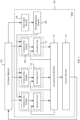
- FIG. 1 shows example NN hardware, which may be referred to as a neural network accelerator (NNA) 100, which implements the NN at run time.
- NNA neural network accelerator
- the compressed coefficients are stored in external memory 102 and are read into a coefficient buffer 104 in the NNA 100.
- the compressed coefficients are then decompressed by a decompression engine 106 and output into a plurality of processing elements 107 that collectively combine the coefficients with the input data for the particular NN layer (which may also be read from the external memory 102) to generate the output data for the NN layer.
- the NN layer is a convolutional layer and hence the processing elements 107 each comprise a convolution engine 108 and an accumulator 110.
- the NNA 100 may also comprise one or more buffers such as an accumulation buffer 112 and an output buffer. As shown in FIG. 1 , the accumulation buffer 112 receives the outputs from the processing elements 107.
- the NNA 100 may also comprise one or more input buffers (not shown in FIG. 1 ) which store the input data after it is read from the external memory 102 and before it is input to the processing elements 107.
- An input to the NN may comprise text data, audio data, video data, or multimodal data - for example text data and image data (such as a caption and an associated image).
- Image processing applications include but are not limited to: image segmentation; image classification; optical character recognition.
- the results of the mapping method comprises data that defines how the coefficients are divided into passes, e.g. in terms of the number of passes or the number of coefficients or filters per pass.
- This method results in a particularly inefficient implementation where the coefficients are sparse (i.e. they comprise many more zeros than ones) because the compression ratio that can be achieved for sparse coefficients is generally higher than for non-sparse coefficients (i.e. sparse coefficients are more compressible).
- the coefficients may be trained, such that their distribution is Gaussian-like or Laplacian-like, which increases the compression ratio that can be achieved (e.g. a compression ratio of around 50% may be achieved).
- the first part 201 of the flow diagram in FIG. 2 shows an example implementation of this method in which the splitting of coefficients is performed at the level of a filter (e.g. such that the smallest split is a single filter).
- This method may also be used where the splitting is performed in a different way (e.g. per compression block or where p-splits are used) and so reference to number of filters in the following description is by way of example only (e.g. it could alternatively refer to the number of blocks or to the number filters multiplied by the number of p-splits where p-splits are used).
- the method takes as input the set of coefficients 202 and the hardware constraint 206 (e.g. the tightest hardware constraint where there are multiple hardware constraints which affect the reading in of the coefficients into the NNA), which may, for example, be the size of the coefficient buffer, cbuf_size. Where the coefficients are quantized, the method may also take as input the size of each quantized coefficient 204 (e.g. in terms of the number of bits per quantized coefficient). The method comprises calculating the number of filters, num_filters (block 208), e.g.
- the output of the method 201 may be the number of filters in each split, init_num_split_filters, or the number of passes (which is given by num_filters divided by init_num_split_filters ) .
- the efficiency of this example method may be improved, as shown in the second part of FIG. 2 .
- the additional method steps comprise taking the results (e.g. the number of filters per pass, init_num_split_filters, or the number of passes) from the analysis based on the uncompressed size 201 and dividing up the set of coefficients into groups, one group for each pass, such that each set comprises the coefficients for the calculated number of filters, (block 214), i.e. initially, each group comprises a number of filters given by init_num_split_filters.
- Each group of coefficients is independently compressed (e.g. using the compression method described in GB 2579399 ) and the largest compressed size of any of the groups of coefficients is identified (block 216).
- num_split_filters init_num_split_filters
- num_split_filters - x the results from the previous iteration, num_split_filters - x, is output (block 220). Again, the value of num_split_filters - x may not divide exactly into num_filters and so all but one split may comprise a number of filters given by num_split_filters - x whilst there may be one split with fewer filters than this.
- the method may start at the top of the tree, jump down a few levels and then move up/down within the tree based on calculated compressed sizes) and the method may start at any depth within the tree.
- exploration of the binary tree may be depth-first or breadth-first.
- the resulting binary tree may be a balanced binary tree (i.e. where all branches terminate at the same depth) or an unbalanced binary tree (i.e. where at least some branches terminate at different depths from other branches in the tree). Whether the tree is balanced or unbalanced may depend upon the compression operation, e.g. how uniform the compression is.
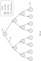
- a binary tree is a tree-like data structure which has binary (i.e. two) splits at each branch and an example of a binary tree is shown in FIG. 3A .
- the tree consists of two types of nodes: split nodes 302 and leaf nodes 304.
- Split nodes 302 are responsible for splitting and passing data to branches 306, whereas leaf nodes 304 terminate branches and may contain information about the data reaching them (e.g. recording the size of split reaching a leaf node).
- the position of a node split or leaf
- At least the largest of the compressed sizes of all the splits is then compared to the hardware constraint(s) (e.g. to the tightest hardware constraint) and the tree is traversed either downwards (such that the current depth increases compared to the starting depth) or upwards (such that the current depth decreases compared to the starting depth) based on the result of that comparison.
- At least one further iteration is performed (splitting the constraints into groups based on the current depth, determining the new compressed group sizes, and comparing at least the maximum compressed size to the hardware constraint) before data defining the coefficient groups is output.
- the data defining the coefficient groups that is output by the improved method described herein splits the layer of the NN into a plurality of passes that are tailored to the specific hardware on which the NN will be executed, with each pass corresponding to a coefficient group. Having output the data defining the coefficient groups, the layer of the NN may be executed on the specific hardware by executing the passes defined by the coefficient groups. As described above, by using the improved method of mapping described herein, not only is the mapping performed more quickly, but also the efficiency of the specific hardware when executing the NN is improved.
- the improved method of mapping a NN onto hardware may be used for a convolutional NN layer (where each coefficient is a weight that belongs to a convolutional filter) or for other types of NN layers where coefficients are combined with input data (e.g. fully connected layers, deconvolution layers, etc.). Any reference to a convolutional NN layer is by way of example only.
- the improved method of mapping a NN onto hardware may be used in combination with the compression method described in GB patent 2579399 or any other block-based compression method where increasing the number of data items in a group of data items that are compressed together cannot result in an increase in the compression ratio that is achieved.
- the method is particularly beneficial where the compression method used does not result in a fixed compression ratio but instead where different groups of data may be compressed by different amounts dependent upon the values of the data items within the group. This is because the compressed size cannot be determined based on the uncompressed size alone (i.e. it cannot be determined without actually performing the compression).
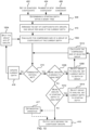
- FIG. 4 A first example of the improved method of mapping a NN onto hardware is shown in FIG. 4 .
- the method takes as input the set of coefficients 402 (where these may be quantized coefficients) and the hardware constraint 406, which may, for example, be the size of the coefficient buffer, cbuf_size.
- FIG. 4 refers to a single hardware constraint it will be appreciated that there may be more than one hardware constraint that is received as input. Where more than one hardware constraint is input, the later comparison operation may use the tightest of those input constraints or may use some or all of the input constraints.
- the method may also take as input the size of each quantized coefficient 404 (e.g. in terms of the number of bits per quantized coefficient). Where this size is not input but is used as part of a subsequent operation, the size may be determined from analysis of the set of coefficients 402.
- the method starts by determining a starting depth within the binary tree (block 408).
- the bottom level may be selected such that each leaf node comprises the smallest split of coefficients.
- the smallest split of coefficients may be determined based on characteristics of the NN layer, e.g. the coefficients that form a single filter in a convolutional NN layer unless p-splits are used. Where p-splits are used, the smallest possible split may be the coefficients that form a single filter from those channels in the p-split. As noted above, where a block passed compression method is used, the coefficients in the smallest possible split may be padded with zeros so that it is a multiple of the block size.
- the selection of the starting depth determines whether the binary tree is traversed in a downwards direction (i.e. such that the depth increases) or an upwards direction (i.e. such that the depth decreases). For example, if the starting depth is 0 or 1, the binary tree is traversed in a downwards direction and if the starting depth is at the bottom of the tree, the binary tree is traversed in an upwards direction. For intermediate starting depths, the binary tree may be traversed either downwards or upwards and this may be dependent upon the way that the starting depth is calculated (e.g. whether the starting depth is calculated to be conservatively small, in which case the traversal is downwards, or conservatively large, in which case the traversal is upwards).
- the input set of coefficients is divided into groups (block 410), with one group for each split node in the determined starting depth (e.g. as calculated using equation 2) and in this initial iteration each group of coefficients is compressed in order to determine the compressed size of each group (block 412). These compressed group sizes are then used to determine whether termination criteria are met (block 414). These termination criteria, which are described in more detail below, differ depending upon whether the binary tree is being traversed downwards or upwards, and involve a comparison of at least one compressed group size to the hardware constraint(s). The termination criteria also ensure that at least two iterations of the method are performed.
- the termination criteria are never met and so the current depth, which is initially equal to the starting depth, is updated (block 416).
- This updating of the current depth may be performed in a number of different ways, e.g. dependent upon whether the binary tree is restricted to being a balanced binary tree or whether the binary tree may be an unbalanced tree and this is described in more detail below.
- the updating also depends on the value of the starting depth and/or how the starting depth was determined and as a result whether the binary tree is being traversed in a downwards direction or an upwards direction.
- the update increases the current depth, whereas if the binary tree is being traversed upwards, the update (in block 416) reduces the current depth.
- the method of FIG. 4 may terminate after two or more iterations when the termination criteria are satisfied (in block 414) and these termination criteria will differ depending upon whether the binary tree is being traversed in a downwards direction or an upwards direction.
- the termination criteria may be given by (equations 6A, 6B, 6C): compressed _ group _ size ⁇ cbuf _ size current _ depth ⁇ starting _ depth + 1 current _ depth ⁇ 2 and the method terminates only if all of these criteria (i.e. all of equations 6A, 6B and 6C) are satisfied.
- the termination criteria may be given by (equations 7A, 7B): compressed _ group _ size ⁇ cbuf _ size current _ depth ⁇ starting _ depth ⁇ 1 and similarly, the method terminates only if all of these criteria (i.e. both equations 7A and 7B) are satisfied. Of these criteria, only the first one (equations 6A and 7A) involve a comparison to the tightest hardware constraint and the second (equations 6B and 7B) ensures that at least two iterations of the method of FIG. 4 are performed.
- data defining the coefficient groups may be output (block 418) based on the current depth at the time of termination or further optimizations may first be performed (block 417), as described below with reference to FIGs. 8-9 .
- the data that is output may define the coefficient groups in a number of different ways and this will depend, in part, on whether a balanced or unbalanced tree is used. For a balanced tree, the output data may define the number of splits or the number of coefficients (or filters or blocks) per split. For an unbalanced tree, data is output that defines each individual split because the splits will not all be the same size and may define the number of coefficients (or filters or blocks) in each individual split.
- the data output (in block 418) specifies the number of hardware passes and how the coefficients are divided into these hardware passes. Having output the data that defines the hardware passes (in block 418), the corresponding passes may be executed on the hardware (i.e. on the hardware with the hardware constraint 406) in order to execute the layer of the NN.
- this value may not divide exactly into num_filters and so all but one split may comprise the same number of filters as specified by the output data (from block 418) whilst there may be one split with fewer filters than this.
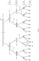
- FIG. 5 shows a schematic diagram of the splitting of a set of coefficients 502 as the tree is traversed downwards.
- Each small square block 503 in FIG. 5 represents the smallest possible split which, as described above, may correspond to the coefficients of a single filter or the coefficients forming a block according to the block-based compression scheme used. It will be appreciated that in practice there will be very many more coefficients than are shown in FIG. 5 .
- the result of the comparison to the hardware constraint (in block 414) is shown by way of shading.
- a group that exceeds the hardware constraint is shown unshaded and a group that satisfies the hardware constraint is shown as shaded.
- each of the groups from the previous iteration are split in two (in block 410) to form eight groups 516-530 and then each of the eight groups are compressed (in block 412) to calculate eight compressed group sizes.
- at least the largest, and in many cases all, of the compressed group sizes are then compared to the hardware constraint (in block 414), although any groups that are derived from groups that did not exceed the constraint in the previous iteration (e.g. that are derived from groups that are shown as shaded in FIG. 5 ) may be excluded from the calculation and comparison operations (blocks 412 and 414) or from only the comparison operation (block 414).
- each of the groups from the previous iteration are split in two (in block 410) to form sixteen groups and then each of the sixteen groups are compressed (in block 412) to calculate sixteen compressed group sizes. At least the largest, and in many cases all, of the compressed group sizes are then compared to the hardware constraint (in block 414). In this example, all of the compressed group sizes satisfy the hardware constraint and so the method terminates ( ⁇ Yes' in block 414) and data defining the coefficient groups at the output depth, where the output depth is given by current_depth and in this example is equal to four, is output (in block 418).
- the number of minimum sized splits 503 in each group may be determined from the output depth using equation 8.
- the termination criteria may be applied on a per-branch basis so that instead of terminating completely after the second iteration, the method only terminates for those branches forming the group 610 that did not satisfy the hardware constraint. For the remaining branches, the binary tree is traversed further upwards, i.e. current_depth is decreased by one (in block 416).
- a pair of groups from the previous iteration are combined (in block 410) to form four groups 622-628. It can be seen that whilst the branches 630, 632 forming group 610 have terminated, group 610 is still used to form one of the four groups 624 in the third iteration.
- the compressed size of each group is calculated (in block 412) and compared to the hardware constraint (in block 414).
- a branch is terminated ( ⁇ Yes' in block 414) if the group does not satisfy the hardware constraint and so in this example, there are three branches 634-638 that terminate because there are two groups 624, 628 that do not satisfy the hardware constraint.
- a pair of groups from the previous iteration are combined (in block 410) to form two groups 644, 646.
- the compressed size of each group is calculated (in block 412) and compared to the hardware constraint (in block 414). As both groups do not satisfy the hardware constraint, all remaining branches terminate ( ⁇ Yes' in block 414).
- the starting depth is calculated by dividing the compressed size by the hardware constraint to give the number of starting splits and then using equation 2 to determine the depth that comprises that number of splits.
- the result is biased to a smaller value to ensure that the starting depth that is used is not too low (in the orientation of FIGs. 3A and 3B ) and where the binary tree is traversed upwards, the result is biased to a larger value so that the starting depth is not too high (in the orientation of FIG. 6 ).
- the resulting depth may be rounded upwards and then the starting depth selected to be one less than the resulting depth or the resulting depth may be rounded downwards and the starting depth selected to be equal to the resulting depth.
- the sizes need to be in the same units (e.g. bits or bytes).
- the resulting depth may be rounded downwards and then the starting depth selected to be one more than the resulting depth or the resulting depth may be rounded upwards and the starting depth selected to be equal to the resulting depth.
- starting depth ⁇ log 2 compressed set size cbuf size ⁇ + 1
- starting _ depth ⁇ log 2 compressed set size cbuf size ⁇
- the current depth may be used directly to output data defining the coefficient groups (in block 418) or one or more optimizations may be performed (in block 417).
- the method of FIG. 4 may in addition, or alternatively, be speeded up by using a larger value of x, such that x>1. This results in skipping layers in the binary tree and whilst it speeds up the operation of the method, the results are more likely to be less optimum and this may reduce the resultant hardware efficiency at run time.
- FIG. 8 A first example optimization is shown in FIG. 8 which corresponds to the second part of FIG. 2 and which may be used for balanced trees.
- this optimization receives the current_depth value and using this, and the direction of traversal, defines the size of each coefficient group, num_split_filters, (block 802).
- the size of each coefficient group may be determined (in block 802) by calculating an interim_depth value from the current_depth value using the same technique as described above to calculate the output depth and then using equation 8. If the tree is being traversed downwards, then the interim_depth is equal to current_depth and if the tree is being traversed upwards, then the interim_depth is given by current_depth + 1.
- the number of filters per split, num_split_filters is increased, e.g. by an integer value, x (block 804, which corresponds to block 219 in FIG. 2 ).
- the group size from the previous iteration (as given by num_split_filters - x) is output and used to generate the output data defining the coefficient groups (in block 418 of FIG. 4 ).
- the group size from the previous iteration (as given by num_split_filters - x) is output and used to generate the output data defining the coefficient groups (in block 418 of FIG. 4 ).
- the final data that is output in block 418) may define a number of filters per split that does not divide exactly into the total number of filters in the layer.
- This first optimization results in a finer granularity of splitting than purely powers of two (as in the method of FIG. 4 without any optimizations) but can be performed much more quickly than using the method of FIG. 2 .
- the optimization method starts in a similar manner to the optimization of FIG. 8 by receiving the current_depth value and using this, and the direction of traversal, to define the size of each coefficient group, num_split_filters, (block 902, which corresponds to block 802 of FIG. 8 ).
- the size of each coefficient group may be determined (in block 902) by calculating an interim_depth value from the current_depth value using the same technique as described above to calculate the output depth and then using equation 8. If the tree is being traversed downwards, then the interim_depth is equal to current_depth and if the tree is being traversed upwards, then the interim_depth is given by current_depth + 1.
- the groups are not merged (block 916). The method may then be repeated by selecting a further two or more groups (in block 908) and comparing the combined compressed size of the newly selected groups to the tightest hardware constraint (in block 912).
- the method determines whether there are any groups at the starting depth that are still to be analysed (block 1012) and if so the method proceeds to analyse that group (as selected in block 1014) and any groups formed by subdivision of that group in a similar manner to the first branch to be explored all the way to the leaf nodes. Only when all branches have been explored (resulting in a 'No' in block 1012) is data output and as before, one or more optimizations may be applied (in block 417) before outputting the data (in block 418). The output data is generated (in block 418) in the same manner for depth-first traversal as for breadth-first traversal (as described above with reference to FIG. 4 ). By defining the coefficient groups, the data output (in block 418) specifies the number of hardware passes and how the coefficients are divided into these hardware passes.
- the coefficients are divided into two groups 504, 506 and the compressed size of group 504 is calculated (in block 1002).
- the termination criteria are not satisfied ('No' in block 414)
- the current depth is increased by x (in block 416).
- the group 504 is therefore split into two groups 508, 510 (in block 1004).
- the compressed size of one of these groups, group 508, is calculated and it is identified that the termination criteria are met, as indicated by the shading in FIG. 5 ( ⁇ Yes' in block 414).
- the resulting tree is inherently unbalanced because the depth at which any branch terminates is independent of other branches in the tree.
- f-splits or p-splits are used and in other examples both f-splits and p-splits may be used (e.g. an f-split may be used in one iteration followed by a p-split in a next iteration).
- p-splits this may affect the merging optimization, as described above with reference to FIG. 9 , by restricting the merging of groups to groups that are adjacent in the binary tree (rather than allowing a totally free selection of groups to merge).
- p-splits are used, intermediate results are saved as higher precision, then loaded in the next pass and accumulated.
- mapping a neural network to the hardware on which it will be implemented at run time.
- the mapping process is performed offline but the way in which it is performed can have performance implications at run time (e.g. in terms of bandwidth, latency, efficiency, power consumption, etc.).
- the mapping process may comprise splitting the layers into the hardware passes using the methods described herein, compressing the coefficients (according to the final split data output from the splitting method) and then generating the converted neural network (e.g. generating a command stream that executes these smaller sets of operations, such as sending corresponding input and weight data to the corresponding buffers, including where necessary, saving intermediate results at higher precision and then performing accumulation of intermediate convolution results).
- the efficiency of the hardware at run time can be significantly increased. For example, an increase of coefficient buffer use from somewhere in the range of 30%-50% (where the splitting is based on the uncompressed sizes) to close to 90% or more may be achieved. As described above, utilising the coefficient buffer more efficiently reduces the overall number of passes that are required which provides benefits such as reduced latency, reduced bandwidth and lower power consumption. For example, the number of passes that are required may be approximately halved. In addition, compared to exploring all possible combinations of splits (i.e. the first of the methods described above), the time taken to perform the offline splitting of the layers (i.e. the coefficients of the layers) into passes may be reduced by 1-2 orders of magnitude.
- the NN hardware of FIG. 1 is shown as comprising a number of functional blocks. This is schematic only and is not intended to define a strict division between different logic elements of such entities. Each functional block may be provided in any suitable manner. It is to be understood that intermediate values described herein as being formed by an element within the NN hardware need not be physically generated by the hardware at any point and may merely represent logical values which conveniently describe the processing performed by the NN hardware between its input and output.
- the NN hardware described herein may be embodied in hardware on an integrated circuit.
- any of the functions, methods, techniques or components described above can be implemented in software, firmware, hardware (e.g., fixed logic circuitry), or any combination thereof.
- the terms “module,” “functionality,” “component”, “element”, “unit”, “block” and “logic” may be used herein to generally represent software, firmware, hardware, or any combination thereof.
- the module, functionality, component, element, unit, block or logic represents program code that performs the specified tasks when executed on a processor.
- the algorithms and methods described herein could be performed by one or more processors executing code that causes the processor(s) to perform the algorithms/methods.
- Examples of a computer-readable storage medium include a random-access memory (RAM), read-only memory (ROM), an optical disc, flash memory, hard disk memory, and other memory devices that may use magnetic, optical, and other techniques to store instructions or other data and that can be accessed by a machine.
- RAM random-access memory
- ROM read-only memory
- optical disc flash memory
- hard disk memory and other memory devices that may use magnetic, optical, and other techniques to store instructions or other data and that can be accessed by a machine.
- a method of manufacturing at an integrated circuit manufacturing system, a NNA as described herein. Furthermore, there may be provided an integrated circuit definition dataset that, when processed in an integrated circuit manufacturing system, causes the method of manufacturing a NNA to be performed.
- An integrated circuit definition dataset may be in the form of computer code, for example as a netlist, code for configuring a programmable chip, as a hardware description language defining an integrated circuit at any level, including as register transfer level (RTL) code, as high-level circuit representations such as Verilog or VHDL, and as low-level circuit representations such as OASIS (RTM) and GDSII.
- RTL register transfer level
- RTM OASIS
- GDSII GDSI
- one or more intermediate user steps may be required in order for a computer system configured for generating a manufacturing definition of an integrated circuit to execute code defining an integrated circuit so as to generate the manufacturing definition of that integrated circuit.
- FIG. 13 shows an example of an integrated circuit (IC) manufacturing system 1302 which is configured to manufacture a NNA as described in any of the examples herein.
- the IC manufacturing system 1302 comprises a layout processing system 1004 and an integrated circuit generation system 1306.
- the IC manufacturing system 1302 is configured to receive an IC definition dataset (e.g. defining a NNA as described in any of the examples herein), process the IC definition dataset, and generate an IC according to the IC definition dataset (e.g. which embodies a NNA as described in any of the examples herein).
- the processing of the IC definition dataset configures the IC manufacturing system 1302 to manufacture an integrated circuit embodying a NNA as described in any of the examples herein.
- the layout processing system 1304 is configured to receive and process the IC definition dataset to determine a circuit layout.
- Methods of determining a circuit layout from an IC definition dataset are known in the art, and for example may involve synthesising RTL code to determine a gate level representation of a circuit to be generated, e.g. in terms of logical components (e.g. NAND, NOR, AND, OR, MUX and FLIP-FLOP components).
- a circuit layout can be determined from the gate level representation of the circuit by determining positional information for the logical components. This may be done automatically or with user involvement in order to optimise the circuit layout.
- the layout processing system 1004 When the layout processing system 1004 has determined the circuit layout it may output a circuit layout definition to the IC generation system 1306.
- a circuit layout definition may be, for example, a circuit layout description.
- the IC generation system 1006 generates an IC according to the circuit layout definition, as is known in the art.
- the IC generation system 1306 may implement a semiconductor device fabrication process to generate the IC, which may involve a multiple-step sequence of photo lithographic and chemical processing steps during which electronic circuits are gradually created on a wafer made of semiconducting material.
- the circuit layout definition may be in the form of a mask which can be used in a lithographic process for generating an IC according to the circuit definition.
- the circuit layout definition provided to the IC generation system 1306 may be in the form of computer-readable code which the IC generation system 1306 can use to form a suitable mask for use in generating an IC.
- the different processes performed by the IC manufacturing system 1302 may be implemented all in one location, e.g. by one party.
- the IC manufacturing system 1002 may be a distributed system such that some of the processes may be performed at different locations, and may be performed by different parties. For example, some of the stages of: (i) synthesising RTL code representing the IC definition dataset to form a gate level representation of a circuit to be generated, (ii) generating a circuit layout based on the gate level representation, (iii) forming a mask in accordance with the circuit layout, and (iv) fabricating an integrated circuit using the mask, may be performed in different locations and/or by different parties.
- processing of the integrated circuit definition dataset at an integrated circuit manufacturing system may configure the system to manufacture a NNA without the IC definition dataset being processed so as to determine a circuit layout.
- an integrated circuit definition dataset may define the configuration of a reconfigurable processor, such as an FPGA, and the processing of that dataset may configure an IC manufacturing system to generate a reconfigurable processor having that defined configuration (e.g. by loading configuration data to the FPGA).
- an integrated circuit manufacturing definition dataset when processed in an integrated circuit manufacturing system, may cause an integrated circuit manufacturing system to generate a device as described herein.
- the configuration of an integrated circuit manufacturing system in the manner described above with respect to FIG. 13 by an integrated circuit manufacturing definition dataset may cause a device as described herein to be manufactured.
- an integrated circuit definition dataset could include software which runs on hardware defined at the dataset or in combination with hardware defined at the dataset.
- the IC generation system may further be configured by an integrated circuit definition dataset to, on manufacturing an integrated circuit, load firmware onto that integrated circuit in accordance with program code defined at the integrated circuit definition dataset or otherwise provide program code with the integrated circuit for use with the integrated circuit.
- a remote computer may store an example of the process described as software.
- a local or terminal computer may access the remote computer and download a part or all of the software to run the program.
- the local computer may download pieces of the software as needed, or execute some software instructions at the local terminal and some at the remote computer (or computer network).
- a dedicated circuit such as a DSP, programmable logic array, or the like.
- the methods described herein may be performed by a computer configured with software in machine readable form stored on a tangible storage medium e.g. in the form of a computer program comprising computer readable program code for configuring a computer to perform the constituent portions of described methods or in the form of a computer program comprising computer program code means adapted to perform all the steps of any of the methods described herein when the program is run on a computer and where the computer program may be embodied on a computer readable storage medium.
- tangible (or non-transitory) storage media include disks, thumb drives, memory cards etc. and do not include propagated signals.
- the software can be suitable for execution on a parallel processor or a serial processor such that the method steps may be carried out in any suitable order, or simultaneously.
- the hardware components described herein may be generated by a non-transitory computer readable storage medium having encoded thereon computer readable program code.
- Non-transitory media can be volatile or non-volatile.
- volatile non-transitory media include semiconductor-based memory, such as SRAM or DRAM.
- technologies that can be used to implement non-volatile memory include optical and magnetic memory technologies, flash memory, phase change memory, resistive RAM.
- logic refers to structure that performs a function or functions.
- An example of logic includes circuitry that is arranged to perform those function(s).
- circuitry may include transistors and/or other hardware elements available in a manufacturing process.
- transistors and/or other elements may be used to form circuitry or structures that implement and/or contain memory, such as registers, flip flops, or latches, logical operators, such as Boolean operations, mathematical operators, such as adders, multipliers, or shifters, and interconnect, by way of example.
- Such elements may be provided as custom circuits or standard cell libraries, macros, or at other levels of abstraction. Such elements may be interconnected in a specific arrangement.
- Logic may include circuitry that is fixed function and circuitry can be programmed to perform a function or functions; such programming may be provided from a firmware or software update or control mechanism.
- Logic identified to perform one function may also include logic that implements a constituent function or sub-process.
- hardware logic has circuitry that implements a fixed function operation, or operations, state machine or process.
- performance improvements may include one or more of increased computational performance, reduced latency, increased throughput, and/or reduced power consumption.
- performance improvements can be traded-off against the physical implementation, thereby improving the method of manufacture. For example, a performance improvement may be traded against layout area, thereby matching the performance of a known implementation but using less silicon. This may be done, for example, by reusing functional blocks in a serialised fashion or sharing functional blocks between elements of the devices, apparatus, modules and/or systems.
Landscapes
- Engineering & Computer Science (AREA)
- Physics & Mathematics (AREA)
- Theoretical Computer Science (AREA)
- Health & Medical Sciences (AREA)
- Life Sciences & Earth Sciences (AREA)
- Biomedical Technology (AREA)
- Biophysics (AREA)
- General Health & Medical Sciences (AREA)
- General Physics & Mathematics (AREA)
- Evolutionary Computation (AREA)
- Computational Linguistics (AREA)
- Molecular Biology (AREA)
- Computing Systems (AREA)
- General Engineering & Computer Science (AREA)
- Data Mining & Analysis (AREA)
- Mathematical Physics (AREA)
- Software Systems (AREA)
- Artificial Intelligence (AREA)
- Neurology (AREA)
- Compression, Expansion, Code Conversion, And Decoders (AREA)
- Character Discrimination (AREA)
- Image Analysis (AREA)
Applications Claiming Priority (1)
| Application Number | Priority Date | Filing Date | Title |
|---|---|---|---|
| GB2209110.2A GB2620113B (en) | 2022-06-21 | 2022-06-21 | Mapping neural networks to hardware |
Publications (1)
| Publication Number | Publication Date |
|---|---|
| EP4296901A1 true EP4296901A1 (de) | 2023-12-27 |
Family
ID=82705539
Family Applications (1)
| Application Number | Title | Priority Date | Filing Date |
|---|---|---|---|
| EP23180122.6A Pending EP4296901A1 (de) | 2022-06-21 | 2023-06-19 | Abbildung von neuronalen netzen auf hardware |
Country Status (4)
| Country | Link |
|---|---|
| US (1) | US20240119254A1 (de) |
| EP (1) | EP4296901A1 (de) |
| CN (1) | CN117273093A (de) |
| GB (1) | GB2620113B (de) |
Citations (3)
| Publication number | Priority date | Publication date | Assignee | Title |
|---|---|---|---|---|
| US20200026992A1 (en) * | 2016-09-29 | 2020-01-23 | Tsinghua University | Hardware neural network conversion method, computing device, compiling method and neural network software and hardware collaboration system |
| US20200177200A1 (en) * | 2018-11-30 | 2020-06-04 | Imagination Technologies Limited | Data Compression and Storage |
| GB2599909A (en) * | 2020-10-13 | 2022-04-20 | Imagination Tech Ltd | Implementation of a neural network in multicore hardware |
Family Cites Families (9)
| Publication number | Priority date | Publication date | Assignee | Title |
|---|---|---|---|---|
| WO2016090568A1 (en) * | 2014-12-10 | 2016-06-16 | Mediatek Singapore Pte. Ltd. | Binary tree block partitioning structure |
| EP3104309B1 (de) * | 2015-06-10 | 2020-04-01 | Samsung Electronics Co., Ltd. | Anreicherung eines neuronalen netzwerks mit reduziertem speicherzugriff und verringertem netzinternem bandbreitenverbrauch |
| CN107533668B (zh) * | 2016-03-11 | 2021-01-26 | 慧与发展有限责任合伙企业 | 用于计算神经网络的节点值的硬件加速器和方法 |
| TWI696961B (zh) * | 2018-12-12 | 2020-06-21 | 財團法人工業技術研究院 | 深度神經網路硬體加速器與其操作方法 |
| US11625584B2 (en) * | 2019-06-17 | 2023-04-11 | Intel Corporation | Reconfigurable memory compression techniques for deep neural networks |
| DE102019218947A1 (de) * | 2019-12-05 | 2021-06-10 | Robert Bosch Gmbh | Hardwarebeschleunigter Betrieb künstlicher neuronaler Netzwerke |
| US12450486B2 (en) * | 2019-12-13 | 2025-10-21 | Qualcomm Incorporated | Depth-first deep convolutional neural network inference |
| US20220414437A1 (en) * | 2019-12-18 | 2022-12-29 | Google Llc | Parameter caching for neural network accelerators |
| JP6834097B1 (ja) * | 2020-05-15 | 2021-02-24 | エッジコーティックス ピーティーイー. リミテッド | 推論のニューラルネットワークアクセラレータのハードウェア固有分割 |
-
2022
- 2022-06-21 GB GB2209110.2A patent/GB2620113B/en active Active
-
2023
- 2023-06-19 EP EP23180122.6A patent/EP4296901A1/de active Pending
- 2023-06-19 CN CN202310728286.4A patent/CN117273093A/zh active Pending
- 2023-06-21 US US18/212,347 patent/US20240119254A1/en active Pending
Patent Citations (4)
| Publication number | Priority date | Publication date | Assignee | Title |
|---|---|---|---|---|
| US20200026992A1 (en) * | 2016-09-29 | 2020-01-23 | Tsinghua University | Hardware neural network conversion method, computing device, compiling method and neural network software and hardware collaboration system |
| US20200177200A1 (en) * | 2018-11-30 | 2020-06-04 | Imagination Technologies Limited | Data Compression and Storage |
| GB2579399A (en) | 2018-11-30 | 2020-06-24 | Imagination Tech Ltd | Data compression and storage |
| GB2599909A (en) * | 2020-10-13 | 2022-04-20 | Imagination Tech Ltd | Implementation of a neural network in multicore hardware |
Non-Patent Citations (1)
| Title |
|---|
| GARCIA A ET AL: "A binary-tree architecture for scheduling real-time systems with hard and soft tasks", INTEGRATED CIRCUITS AND SYSTEMS DESIGN, 1999. PROCEEDINGS. XII SYMPOSI UM ON NATAL, BRAZIL 29 SEPT.-2 OCT. 1999, LOS ALAMITOS, CA, USA,IEEE COMPUT. SOC, US, 29 September 1999 (1999-09-29), pages 78 - 81, XP010355762, ISBN: 978-0-7695-0387-5, DOI: 10.1109/SBCCI.1999.802972 * |
Also Published As
| Publication number | Publication date |
|---|---|
| US20240119254A1 (en) | 2024-04-11 |
| CN117273093A (zh) | 2023-12-22 |
| GB2620113B (en) | 2024-09-18 |
| GB2620113A (en) | 2024-01-03 |
| GB202209110D0 (en) | 2022-08-10 |
Similar Documents
| Publication | Publication Date | Title |
|---|---|---|
| US20220391172A1 (en) | Implementation of Softmax and Exponential in Hardware | |
| US20250068898A1 (en) | Neural network architecture using single plane filters | |
| US20240137044A1 (en) | Data compression and storage | |
| EP3242253B1 (de) | Hardwareimplementierung eines neuronalen konvolutionsnetzwerks | |
| EP4160485A1 (de) | Verfahren und vorrichtungen zur konfiguration eines beschleunigers eines neuronalen netzwerks mit einer konfigurierbaren pipeline | |
| EP4024291B1 (de) | Neuronales netzwerk mit matrixmultiplikation | |
| US20230019151A1 (en) | Implementation of pooling and unpooling or reverse pooling in hardware | |
| US20230021204A1 (en) | Neural network comprising matrix multiplication | |
| CN113887714B (zh) | 用于在硬件中运行动态循环神经网络的方法、系统和介质 | |
| EP4345691A1 (de) | Verfahren und systeme zur durchführung von kanalentzerrung auf einer faltungsschicht in einem neuronalen netzwerk | |
| US20240143986A1 (en) | Methods and systems for executing a neural network on a neural network accelerator | |
| EP4296901A1 (de) | Abbildung von neuronalen netzen auf hardware | |
| US20250322221A1 (en) | Attention-based neural networks | |
| EP4390770A1 (de) | Abbildung von neuronalen netzen auf hardware | |
| EP4390768A1 (de) | Implementierung neuronaler netze in hardware | |
| GB2637252A (en) | Implementing neural networks in hardware |
Legal Events
| Date | Code | Title | Description |
|---|---|---|---|
| PUAI | Public reference made under article 153(3) epc to a published international application that has entered the european phase |
Free format text: ORIGINAL CODE: 0009012 |
|
| STAA | Information on the status of an ep patent application or granted ep patent |
Free format text: STATUS: THE APPLICATION HAS BEEN PUBLISHED |
|
| AK | Designated contracting states |
Kind code of ref document: A1 Designated state(s): AL AT BE BG CH CY CZ DE DK EE ES FI FR GB GR HR HU IE IS IT LI LT LU LV MC ME MK MT NL NO PL PT RO RS SE SI SK SM TR |
|
| STAA | Information on the status of an ep patent application or granted ep patent |
Free format text: STATUS: REQUEST FOR EXAMINATION WAS MADE |
|
| 17P | Request for examination filed |
Effective date: 20240325 |
|
| RBV | Designated contracting states (corrected) |
Designated state(s): AL AT BE BG CH CY CZ DE DK EE ES FI FR GB GR HR HU IE IS IT LI LT LU LV MC ME MK MT NL NO PL PT RO RS SE SI SK SM TR |