EP4150316B1 - Verfahren zum abschnittsweisen bestimmen des volumens eines auf ein förderband aufgegebenen schüttgutes - Google Patents
Verfahren zum abschnittsweisen bestimmen des volumens eines auf ein förderband aufgegebenen schüttgutes Download PDFInfo
- Publication number
- EP4150316B1 EP4150316B1 EP21726034.8A EP21726034A EP4150316B1 EP 4150316 B1 EP4150316 B1 EP 4150316B1 EP 21726034 A EP21726034 A EP 21726034A EP 4150316 B1 EP4150316 B1 EP 4150316B1
- Authority
- EP
- European Patent Office
- Prior art keywords
- depth
- bulk material
- volume
- training
- depth image
- Prior art date
- Legal status (The legal status is an assumption and is not a legal conclusion. Google has not performed a legal analysis and makes no representation as to the accuracy of the status listed.)
- Active
Links
Images

Classifications
-
- G—PHYSICS
- G01—MEASURING; TESTING
- G01N—INVESTIGATING OR ANALYSING MATERIALS BY DETERMINING THEIR CHEMICAL OR PHYSICAL PROPERTIES
- G01N15/00—Investigating characteristics of particles; Investigating permeability, pore-volume or surface-area of porous materials
- G01N15/02—Investigating particle size or size distribution
- G01N15/0205—Investigating particle size or size distribution by optical means
- G01N15/0227—Investigating particle size or size distribution by optical means using imaging; using holography
-
- G—PHYSICS
- G01—MEASURING; TESTING
- G01N—INVESTIGATING OR ANALYSING MATERIALS BY DETERMINING THEIR CHEMICAL OR PHYSICAL PROPERTIES
- G01N15/00—Investigating characteristics of particles; Investigating permeability, pore-volume or surface-area of porous materials
- G01N15/10—Investigating individual particles
- G01N15/14—Optical investigation techniques, e.g. flow cytometry
- G01N15/1429—Signal processing
- G01N15/1433—Signal processing using image recognition
-
- G—PHYSICS
- G01—MEASURING; TESTING
- G01N—INVESTIGATING OR ANALYSING MATERIALS BY DETERMINING THEIR CHEMICAL OR PHYSICAL PROPERTIES
- G01N15/00—Investigating characteristics of particles; Investigating permeability, pore-volume or surface-area of porous materials
- G01N15/10—Investigating individual particles
- G01N15/14—Optical investigation techniques, e.g. flow cytometry
- G01N15/1468—Optical investigation techniques, e.g. flow cytometry with spatial resolution of the texture or inner structure of the particle
- G01N15/147—Optical investigation techniques, e.g. flow cytometry with spatial resolution of the texture or inner structure of the particle the analysis being performed on a sample stream
-
- G—PHYSICS
- G06—COMPUTING OR CALCULATING; COUNTING
- G06F—ELECTRIC DIGITAL DATA PROCESSING
- G06F18/00—Pattern recognition
- G06F18/20—Analysing
- G06F18/24—Classification techniques
- G06F18/241—Classification techniques relating to the classification model, e.g. parametric or non-parametric approaches
- G06F18/2413—Classification techniques relating to the classification model, e.g. parametric or non-parametric approaches based on distances to training or reference patterns
- G06F18/24133—Distances to prototypes
-
- G—PHYSICS
- G06—COMPUTING OR CALCULATING; COUNTING
- G06N—COMPUTING ARRANGEMENTS BASED ON SPECIFIC COMPUTATIONAL MODELS
- G06N3/00—Computing arrangements based on biological models
- G06N3/02—Neural networks
- G06N3/04—Architecture, e.g. interconnection topology
- G06N3/045—Combinations of networks
-
- G—PHYSICS
- G06—COMPUTING OR CALCULATING; COUNTING
- G06N—COMPUTING ARRANGEMENTS BASED ON SPECIFIC COMPUTATIONAL MODELS
- G06N3/00—Computing arrangements based on biological models
- G06N3/02—Neural networks
- G06N3/04—Architecture, e.g. interconnection topology
- G06N3/0464—Convolutional networks [CNN, ConvNet]
-
- G—PHYSICS
- G06—COMPUTING OR CALCULATING; COUNTING
- G06N—COMPUTING ARRANGEMENTS BASED ON SPECIFIC COMPUTATIONAL MODELS
- G06N3/00—Computing arrangements based on biological models
- G06N3/02—Neural networks
- G06N3/08—Learning methods
- G06N3/09—Supervised learning
-
- G—PHYSICS
- G06—COMPUTING OR CALCULATING; COUNTING
- G06T—IMAGE DATA PROCESSING OR GENERATION, IN GENERAL
- G06T7/00—Image analysis
- G06T7/0002—Inspection of images, e.g. flaw detection
- G06T7/0004—Industrial image inspection
-
- G—PHYSICS
- G06—COMPUTING OR CALCULATING; COUNTING
- G06T—IMAGE DATA PROCESSING OR GENERATION, IN GENERAL
- G06T7/00—Image analysis
- G06T7/50—Depth or shape recovery
-
- G—PHYSICS
- G06—COMPUTING OR CALCULATING; COUNTING
- G06T—IMAGE DATA PROCESSING OR GENERATION, IN GENERAL
- G06T7/00—Image analysis
- G06T7/60—Analysis of geometric attributes
- G06T7/62—Analysis of geometric attributes of area, perimeter, diameter or volume
-
- G—PHYSICS
- G06—COMPUTING OR CALCULATING; COUNTING
- G06V—IMAGE OR VIDEO RECOGNITION OR UNDERSTANDING
- G06V10/00—Arrangements for image or video recognition or understanding
- G06V10/20—Image preprocessing
- G06V10/26—Segmentation of patterns in the image field; Cutting or merging of image elements to establish the pattern region, e.g. clustering-based techniques; Detection of occlusion
- G06V10/267—Segmentation of patterns in the image field; Cutting or merging of image elements to establish the pattern region, e.g. clustering-based techniques; Detection of occlusion by performing operations on regions, e.g. growing, shrinking or watersheds
-
- G—PHYSICS
- G06—COMPUTING OR CALCULATING; COUNTING
- G06V—IMAGE OR VIDEO RECOGNITION OR UNDERSTANDING
- G06V10/00—Arrangements for image or video recognition or understanding
- G06V10/70—Arrangements for image or video recognition or understanding using pattern recognition or machine learning
- G06V10/82—Arrangements for image or video recognition or understanding using pattern recognition or machine learning using neural networks
-
- G—PHYSICS
- G06—COMPUTING OR CALCULATING; COUNTING
- G06V—IMAGE OR VIDEO RECOGNITION OR UNDERSTANDING
- G06V20/00—Scenes; Scene-specific elements
- G06V20/50—Context or environment of the image
- G06V20/52—Surveillance or monitoring of activities, e.g. for recognising suspicious objects
-
- G—PHYSICS
- G06—COMPUTING OR CALCULATING; COUNTING
- G06V—IMAGE OR VIDEO RECOGNITION OR UNDERSTANDING
- G06V20/00—Scenes; Scene-specific elements
- G06V20/60—Type of objects
- G06V20/64—Three-dimensional objects
-
- G—PHYSICS
- G01—MEASURING; TESTING
- G01N—INVESTIGATING OR ANALYSING MATERIALS BY DETERMINING THEIR CHEMICAL OR PHYSICAL PROPERTIES
- G01N15/00—Investigating characteristics of particles; Investigating permeability, pore-volume or surface-area of porous materials
- G01N15/10—Investigating individual particles
- G01N15/14—Optical investigation techniques, e.g. flow cytometry
- G01N2015/1497—Particle shape
-
- G—PHYSICS
- G06—COMPUTING OR CALCULATING; COUNTING
- G06T—IMAGE DATA PROCESSING OR GENERATION, IN GENERAL
- G06T2207/00—Indexing scheme for image analysis or image enhancement
- G06T2207/10—Image acquisition modality
- G06T2207/10028—Range image; Depth image; 3D point clouds
-
- G—PHYSICS
- G06—COMPUTING OR CALCULATING; COUNTING
- G06T—IMAGE DATA PROCESSING OR GENERATION, IN GENERAL
- G06T2207/00—Indexing scheme for image analysis or image enhancement
- G06T2207/20—Special algorithmic details
- G06T2207/20081—Training; Learning
-
- G—PHYSICS
- G06—COMPUTING OR CALCULATING; COUNTING
- G06T—IMAGE DATA PROCESSING OR GENERATION, IN GENERAL
- G06T2207/00—Indexing scheme for image analysis or image enhancement
- G06T2207/20—Special algorithmic details
- G06T2207/20084—Artificial neural networks [ANN]
-
- G—PHYSICS
- G06—COMPUTING OR CALCULATING; COUNTING
- G06T—IMAGE DATA PROCESSING OR GENERATION, IN GENERAL
- G06T2207/00—Indexing scheme for image analysis or image enhancement
- G06T2207/30—Subject of image; Context of image processing
- G06T2207/30108—Industrial image inspection
- G06T2207/30164—Workpiece; Machine component
-
- G—PHYSICS
- G06—COMPUTING OR CALCULATING; COUNTING
- G06V—IMAGE OR VIDEO RECOGNITION OR UNDERSTANDING
- G06V2201/00—Indexing scheme relating to image or video recognition or understanding
- G06V2201/06—Recognition of objects for industrial automation
Definitions
- the invention relates to a method for determining the volume of a bulk material fed onto a conveyor belt in sections, wherein a depth image of the bulk material is recorded in sections in a detection area by a depth sensor.
- US 2017/058620 A1 also discloses a method for determining the volume of a bulk material fed onto a conveyor belt in sections.
- the invention is therefore based on the object of reliably classifying bulk material even in the case of overlaps at conveying speeds of more than 2 m/s, without the need for complex structural measures.
- the invention solves the problem by feeding the captured two-dimensional depth image to a pre-trained, convolutional neural network that has at least three consecutive convolution layers, so-called convolution layers, and a downstream volume classifier, for example a so-called fully connected layer, whose output value is output as the bulk material volume present in the detection area.
- the invention is therefore based on the idea that when using two-dimensional depth images, the information required to determine the volume can be extracted from the depth information after a neural network used for this purpose has been trained with training depth images with a known bulk material volume.
- the convolution layers reduce the input depth images to a series of individual features, which in turn are evaluated by the downstream volume classifier, so that the total volume of the material depicted in the input depth image can be determined as a result.
- the number of convolution layers provided can be at least three, preferably five, depending on the available computing power.
- a layer for dimension reduction a so-called flattening layer, can be provided in the known manner. The volume therefore no longer has to be calculated for each individual grain. Since the distance of the object depicted to the depth sensor is depicted with only one value for each pixel in the depth image, In contrast to the processing of color images, the amount of data to be processed is reduced, the measurement process is accelerated and the memory required for the neural network is reduced. This means that the neural network can be implemented on inexpensive AI parallel processing units with GPU support and the process can be used regardless of the color of the bulk material.
- the volume of the bulk material can also be determined by accelerating the measurement process even at conveyor belt speeds of 3m/s, preferably 4m/s. This reduction in the amount of data in the image also reduces the susceptibility to errors in correctly determining the volume of the bulk material.
- the use of depth images has the additional advantage that the measurement process is largely independent of changing exposure conditions.
- a vgg16 network Simonyan / Zisserman, Very Deep Convolutional Networks for Large-Scale Image Recognition, 2015 ) can be used, which is reduced to just one channel, namely for the values of the depth image points.
- the depth image can be captured, for example, with a 3D camera, since this can be positioned above a conveyor belt even when space is limited due to the smaller space requirement.
- several consecutive output values can also be averaged and the average value output as the bulk material volume present in the recording area.
- Training the neural network is made more difficult and measurement accuracy decreases during operation if non-bulk material elements are in the detection range of the depth sensor. These include, for example, vibrating components of the conveyor belt itself or other machine elements. To avoid the resulting interference, it is suggested that the values of those pixels whose depth corresponds to a previously recorded distance between the depth sensor and a background for this pixel are removed from the depth image and/or the training depth image. or exceeds this distance. This allows disturbing image information, caused for example by vibrations of the conveyor belt, to be removed and both the depth images and the training images to be limited to the information relevant for the measurement.
- the bulk material volume alone is not sufficient to determine process parameters, such as those required in particular for use in crushers. It is therefore proposed that a quantity classifier be placed downstream of the convolution levels for each class of a grain size distribution and that the output values of these quantity classifiers be output as a grain size distribution.
- This grain size distribution is a histogram that can be formed either with absolute quantity values or with relative quantity values related to the bulk material volume and thus provides important conclusions, for example on the crushing gap, any faults or other process parameters of a crusher.
- the measures according to the invention can therefore be used to automatically record the sieve curve of crushers at high speeds, which is traditionally only very laborious to determine, since no parameters for individual grains have to be recorded and relevant sizes calculated from them. Determining the grain size distribution directly from the depth image also reduces the susceptibility to errors when determining the grain size distribution.
- Cubicity is considered to be the axial ratio of individual grains of the bulk material, which is, for example, the quotient of the length and thickness of the grain.
- Training the neural network requires large amounts of training depth images that represent the bulk material to be detected as accurately as possible. However, the amount of work required to measure the required amount of bulk material is extremely high. In order to still provide the neural network with In order to provide sufficient training depth images to determine the bulk material volume, it is proposed that example depth images of one example grain with a known volume are first recorded and saved together with the volume, after which several example depth images are randomly combined to form a training depth image, to which the sum of the volumes of the combined example depth images is assigned as the bulk material volume, after which the training depth image is fed to the neural network on the input side and the assigned bulk material volume on the output side, and the weights of the individual network nodes are adjusted in a learning step.
- the training method is therefore based on the idea that by combining example depth images of measured example grains, a variety of combinations of training depth images can be created. It is therefore sufficient to record example depth images of relatively few example grains with their volume in order to generate a large number of training depth images with which the neural network can be trained.
- the weights between the individual network nodes are adjusted in the individual training steps in a known manner so that the actual output value corresponds as closely as possible to the specified output value at the end of the neural network.
- Different activation functions can be specified at the network nodes, which determine whether a total value at the network node is passed on to the next level of the neural network.
- Analogous to the volume other parameters such as cubicity, foreign matter or contaminant content or grain size can also be assigned to the sample depth images.
- the grain size distribution resulting from the grains in the sample depth images can also be assigned to each training depth image.
- the training depth images and the depth images of the measured bulk material only contain the information relevant for the measurement, which results in a more stable Training behavior is achieved and the recognition rate is increased during use.
- the neural network can be trained on any type of bulk material by selecting the example images or the training depth images composed of them.
- the sample depth images with random orientation are assembled into a training depth image. This significantly increases the number of possible arrangements of the grains for a given number of grains per sample depth image without having to generate more sample depth images and overfitting of the neural network is avoided.
- Separation of the grains of the bulk material can be omitted and larger bulk material volumes can be determined at a constant conveyor belt speed if the sample depth images with partial overlaps are combined to form a training depth image, whereby the depth value of the training depth image in the overlap area corresponds to the smallest depth of both sample depth images.
- the neural network can be trained to recognize such overlaps and still be able to determine the volume of the sample grains.
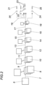
- Fig. 1 shows a device for carrying out the method according to the invention, which comprises a conveyor belt 1 on which bulk material 2 has been placed.
- a depth sensor 3 creates depth images 6 of the bulk material 2 in a detection area 4 of the depth sensor 3 and sends them to a computing unit 5.
- the depth images are fed to a neural network and processed by it.
- the determination of the bulk material volume can include the following steps, for example, and is carried out for a depth image 6 in the Fig. 2 shown:
- a first step 7 the depth image 6 is fed to the first convolution layer.
- several outputs 8, so-called feature maps, which depict different aspects, are generated from the depth image 6 by pixel-by-pixel convolution of the depth image 6 with a convolution kernel. These outputs 8 have the same dimensions and the same number of pixels as the depth image 6.
- the next step 9 the number of pixels is reduced using a pooling layer.
- Steps 7 and 9 are now repeated in further layers, but in step 11 the convolution is applied to each output 10, which further increases the number of outputs 12 generated.
- the application of the pooling layer to the outputs 12 in step 13 further reduces the number of pixels and produces the outputs 14.
- Step 15 is analogous to step 11 and produces the outputs 16.
- Step 17 is analogous to step 13, reduces the number of pixels and produces output 18.
- the application steps of the convolution and pooling layers can be repeated further depending on the aspects to be determined in the depth image 6.
- step 19 the pixels of the outputs 18 are arranged in a row by dimensional reduction and their information is transmitted to a classifier, for example to a volume classifier 20, whose output value 21 can be output as the volume of bulk material present in the detection area.
- a volume classifier 20 whose output value 21 can be output as the volume of bulk material present in the detection area.
- additional quantity classifiers 22 can be used.
- output values 23 form the relative or absolute quantities of the histogram of a grain size distribution.
- a cubicity classifier 24 can also be provided, whose output value 25 corresponds to the average cubicity of the bulk material 2 present in the detection area.
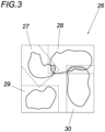
- a training depth image 26 can be seen in the Fig. 3
- four sample depth images 27, 28, 29, 30 of different previously measured grains are put together to form a training depth image 25.
- the sample depth images 27, 28, 29, 30 can be put together in any position and orientation to form a training depth image 26 and can partially overlap.
- the overlaps are shown hatched in the training depth image 26.
Landscapes
- Engineering & Computer Science (AREA)
- Physics & Mathematics (AREA)
- Theoretical Computer Science (AREA)
- General Physics & Mathematics (AREA)
- General Health & Medical Sciences (AREA)
- Chemical & Material Sciences (AREA)
- Health & Medical Sciences (AREA)
- Life Sciences & Earth Sciences (AREA)
- Multimedia (AREA)
- Evolutionary Computation (AREA)
- Computer Vision & Pattern Recognition (AREA)
- Artificial Intelligence (AREA)
- Immunology (AREA)
- Pathology (AREA)
- Biochemistry (AREA)
- Data Mining & Analysis (AREA)
- Analytical Chemistry (AREA)
- Computing Systems (AREA)
- Dispersion Chemistry (AREA)
- Software Systems (AREA)
- General Engineering & Computer Science (AREA)
- Biophysics (AREA)
- Biomedical Technology (AREA)
- Mathematical Physics (AREA)
- Molecular Biology (AREA)
- Computational Linguistics (AREA)
- Medical Informatics (AREA)
- Databases & Information Systems (AREA)
- Geometry (AREA)
- Signal Processing (AREA)
- Quality & Reliability (AREA)
- Bioinformatics & Cheminformatics (AREA)
- Evolutionary Biology (AREA)
- Bioinformatics & Computational Biology (AREA)
- Image Analysis (AREA)
- Length Measuring Devices By Optical Means (AREA)
- Image Processing (AREA)
Description
- Die Erfindung bezieht sich auf ein Verfahren zum abschnittsweisen Bestimmen des Volumens eines auf ein Förderband aufgegebenen Schüttgutes wobei vom Schüttgut abschnittsweise in einem Erfassungsbereich von einem Tiefensensor ein Tiefenbild erfasst wird.
- Es ist bekannt (
WO2006027802A1 ) mittels Dualkamera und Lasertriangulation Schüttgut auf einem Förderband zu vermessen und dessen Eigenschaften, wie das Volumen oder die Geometrie des Schüttgutes aus den Messdaten zu errechnen und zu klassifizieren. - Nachteilig am Stand der Technik ist allerdings, dass diese photogrammetrischen Verfahren sehr zeitaufwändig in der Volumenbestimmung des Schüttgutes sind, da für jedes erfasste Korn im Schüttgut eine Reihe komplizierter Erfassungs- und Vermessungsalgorithmen durchgeführt werden muss, die aufgrund der hohen Kornanzahl und dem individuellen Rechenaufwand pro Korn in Summe hohe Rechenzeiten erfordern. Darüber hinaus dürfen sich bei diesem Verfahren die Körner auf dem Förderband nicht überlappen, was allerdings im realistischen Förderbetrieb unvermeidbar ist. Aufgrund dieser Einschränkungen können im Stand der Technik nur ca. 100-200 Körner pro Stunde vermessen werden. Da übliche Förderbänder bei weitem mehr Körner transportieren als Verfahren aus dem Stand der Technik im selben Zeitraum vermessen können, resultiert die Anwendung bekannter Messverfahren in einer signifikanten Verlangsamung der Fördergeschwindigkeit und damit in Produktivitätseinbußen. Selbst bei aufwändigen Systemen, die einen großen Platzbedarf aufweisen, können so nur
- Bandgeschwindigkeiten von unter 2 m/s erreicht werden.
US 2017/058620 A1 offenbart ebenfalls ein Verfahren zum abschnittsweisen Bestimmen des Volumens eines auf ein Förderband aufgegebenen Schüttgutes. - Der Erfindung liegt somit die Aufgabe zugrunde, Schüttgut auch bei Überlappungen zuverlässig bei Fördergeschwindigkeiten von mehr als 2 m/s zu klassifizieren, ohne dass hierfür konstruktiv aufwendige Maßnahmen getroffen werden müssen.
- Die Erfindung löst die gestellte Aufgabe dadurch, dass das erfasste zweidimensionale Tiefenbild einem vorab trainierten, faltenden neuronalen Netzwerk zugeführt wird, dass wenigstens drei hintereinanderliegende Faltungsebenen, sogenannte convolution layer, und einen nachgelagerten Volumenklassifizierer, beispielsweise ein sogenannter fully connected layer, aufweist, dessen Ausgangswert als das im Erfassungsbereich vorhandene Schüttgutvolumen ausgegeben wird. Der Erfindung liegt also die Überlegung zugrunde, dass bei der Verwendung von zweidimensionalen Tiefenbildern die zur Volumenbestimmung notwendige Information aus den Tiefeninformationen extrahiert werden kann, nachdem ein hierfür eingesetztes neuronales Netzwerk mit Trainingstiefenbildern mit bekanntem Schüttgutvolumen trainiert wurde. Die Faltungsebenen reduzieren dabei die Eingangstiefenbilder zu einer Reihe von Einzelmerkmalen, die wiederum vom nachgelagerten Volumenklassifizierer bewertet werden, sodass im Ergebnis das Gesamtvolumen des im Eingangstiefenbild abgebildeten Materials ermittelt werden kann. Die Anzahl der vorgesehenen Faltungsebenen, die jeweils von einer Pooling-Ebene zur Informationsreduktion gefolgt sein können, kann je nach verfügbarer Rechenleistung bei wenigstens drei, vorzugsweise bei fünf, liegen. Zwischen den Faltungsebenen und dem nachgelagerten Volumenklassifizierer kann in bekannter Weise eine Ebene zur Dimensionsreduktion, ein sogenannter flattening layer, vorgesehen sein. Das Volumen muss daher nicht mehr für jedes einzelne Korn berechnet werden. Da im Tiefenbild je Bildpunkt der Abstand des abgebildeten Objekts zum Tiefensensor mit nur einem Wert abgebildet wird, kann im Gegensatz zur Verarbeitung von Farbbildern die zu verarbeitende Datenmenge reduziert, das Messverfahren beschleunigt und der für das neuronale Netzwerk erforderliche Speicherbedarf verringert werden. Dadurch kann das neuronale Netzwerk auf günstigen KI-Parallelrecheneinheiten mit GPU-Unterstützung implementiert und das Verfahren unabhängig von der Farbe des Schüttgutes eingesetzt werden. Auch kann das Schüttgutvolumen durch die Beschleunigung des Messverfahrens selbst bei Förderbandgeschwindigkeiten von 3m/s, bevorzugter Weise 4m/s, bestimmt werden. Diese Reduktion der Datenmenge im Bild senkt zusätzlich die Fehleranfälligkeit für die korrekte Bestimmung des Schüttgutvolumens. Die Verwendung von Tiefenbildern hat im Gegensatz zu Farb- oder Graustufenbildern den zusätzlichen Vorteil, dass das Messverfahren weitgehend unabhängig von sich ändernden Belichtungsbedingungen ist. Als neuronales Netzwerk kann beispielsweise ein üblicherweise nur für Farbbilder verwendetes vgg16 Netzwerk (Simonyan / Zisserman, Very Deep Convolutional Networks for Large-Scale Image Recognition, 2015) zum Einsatz kommen, das lediglich auf einen Kanal, nämlich für die Werte der Tiefenbildpunkte, reduziert ist. Das Tiefenbild kann beispielsweise mit einer 3D-Kamera erfasst werden, da diese aufgrund des geringeren Platzbedarfes auch bei geringem Raumangebot oberhalb eines Förderbandes angeordnet werden kann. Um Schwankungen bei der Erfassung des Volumens auszugleichen und fehlerhafte Ausgabewerte des neuronalen Netzwerkes zu kompensieren, können darüber hinaus mehrere aufeinanderfolgende Ausgangswerte gemittelt und der Mittelwert als das im Erfassungsbereich vorhandene Schüttgutvolumen ausgegeben werden.
- Das Trainieren des neuronalen Netzwerks wird erschwert und die Messgenauigkeit nimmt im laufenden Betrieb ab, wenn schüttgutfremde Elemente im Erfassungsbereich des Tiefensensors liegen. Dazu zählen beispielsweise vibrierende Bauteile des Förderbandes selbst, oder aber andere Maschinenelemente. Zur Vermeidung der daraus entstehenden Störungen wird vorgeschlagen, dass aus dem Tiefenbild und/oder dem Trainingstiefenbild die Werte jener Bildpunkte entfernt werden, deren Tiefe einem vorab erfassten Abstand zwischen Tiefensensor und einem Hintergrund für diesen Bildpunkt entspricht oder diesen Abstand überschreitet. Dadurch können störende Bildinformationen, hervorgerufen beispielsweise durch Vibrationen des Förderbandes, entfernt und sowohl die Tiefenbilder als auch die Trainingsbilder auf die für die Vermessung relevanten Informationen beschränkt werden.
- Das Schüttgutvolumen reicht allerdings für sich alleine nicht aus, um Prozessparameter, wie sie insbesondere bei der Verwendung in Brechern erforderlich sind, zu ermitteln. Daher wird vorgeschlagen, dass den Faltungsebenen je Klasse einer Korngrößenverteilung ein Mengenklassifizierer nachgelagert ist und die Ausgangswerte dieser Mengenklassifizierer als Korngrößenverteilung ausgegeben werden. Diese Korngrößenverteilung ist ein Histogramm, das entweder mit absoluten Mengenwerten oder aber mit auf das Schüttgutvolumen bezogenen relativen Mengenwerten gebildet werden kann und liefert damit wichtige Rückschlüsse, beispielsweise auf den Brechspalt, etwaige Störungen oder andere Prozessparameter eines Brechers. Somit kann durch die erfindungsgemäßen Maßnahmen die herkömmlicherweise nur sehr aufwändig bestimmbare Siebkurve von Brechern mit hohen Geschwindigkeiten automatisiert erfasst werden, da keine Parameter für einzelne Körner erfasst und daraus relevante Größen berechnet werden müssen. Die Bestimmung der Korngrößenverteilung direkt aus dem Tiefenbild verringert dadurch auch die Fehleranfälligkeit beim Bestimmen der Korngrößenverteilung.
- Um das Schüttgut anhand seiner mechanischen Eigenschaften besser einteilen zu können, wird vorgeschlagen, dass den Faltungsebenen ein Kubizitätsklassifizierer nachgelagert ist, dessen Ausgangswert als Kubizität ausgegeben wird. Als Kubizität wird das Achsenverhältnis einzelner Körner des Schüttguts angesehen, das beispielsweise der Quotient aus Länge und Dicke des Korns ist.
- Das Training des neuronalen Netzwerks erfordert große Mengen an Trainingstiefenbildern, die das zu erfassende Schüttgut möglichst exakt repräsentieren. Der Arbeitsaufwand um die notwendige Menge an Schüttgut zu vermessen ist allerdings extrem hoch. Um dem neuronalen Netz dennoch ausreichende Trainingstiefenbilder zur Verfügung zu stellen, um das Schüttgutvolumen zu bestimmen, wird vorgeschlagen, dass zunächst Beispieltiefenbilder je eines Beispielkornes mit bekanntem Volumen erfasst und gemeinsam mit dem Volumen abgespeichert werden, wonach mehrere Beispieltiefenbilder zufällig zu einem Trainingstiefenbild zusammengesetzt werden, dem als Schüttgutvolumen die Summe der Volumina der zusammengesetzten Beispieltiefenbilder zugeordnet wird, wonach das Trainingstiefenbild eingangsseitig und das zugeordnete Schüttgutvolumen ausgangsseitig dem neuronalen Netzwerk zugeführt und die Gewichte der einzelnen Netzwerkknoten in einem Lernschritt angepasst werden. Der Trainingsmethode liegt also die Überlegung zugrunde, dass durch die Kombination von Beispieltiefenbildern vermessener Beispielkörner mannigfaltige Kombinationen an Trainingstiefenbildern erstellt werden können. Es genügt also, Beispieltiefenbilder verhältnismäßig weniger Beispielkörner mit ihrem Volumen zu erfassen, um eine große Anzahl an Trainingstiefenbildern zu generieren mit denen das neuronale Netzwerk trainiert werden kann. Zum Training des neuronalen Netzwerks werden in den einzelnen Trainingsschritten in bekannter Weise die Gewichte zwischen den einzelnen Netzwerkknoten so angepasst, dass der tatsächliche Ausgabewert dem vorgegebenen Ausgabewert am Ende des neuronalen Netzwerks ehestmöglich entspricht. Dabei können an den Netzwerkknoten unterschiedliche Aktivierungsfunktionen vorgegeben werden, die dafür maßgeblich sind, ob ein am Netzwerkknoten anliegender Summenwert an die nächste Ebene des neuronalen Netzwerks weitergegeben wird. Analog zum Volumen können den Beispieltiefenbildern auch andere Parameter, wie beispielsweise die Kubizität, Fremdstoff- bzw. Störstoffanteil oder die Korngröße zugewiesen werden. Auch kann für jedes Trainingstiefenbild die sich aus den Körnern der Beispieltiefenbilder ergebende Korngrößenverteilung zugewiesen werden. Zur Tiefenbildverarbeitung wird auch hier vorgeschlagen, dass aus dem Tiefenbild die Werte jener Bildpunkte entfernt werden, deren Tiefe einem vorab erfassten Abstand zwischen Tiefensensor und Förderband für diesen Bildpunkt entspricht oder diesen Abstand überschreitet. Dadurch weisen die Trainingstiefenbilder und die Tiefenbilder des gemessenen Schüttguts nur die für die Vermessung relevanten Informationen auf, wodurch ein stabileres Trainingsverhalten erreicht und die Erkennungsrate bei der Anwendung erhöht wird. Über die Auswahl der Beispiel- bzw. der aus ihnen zusammengesetzten Trainingstiefenbilder kann das neuronale Netz auf beliebige Arten von Schüttgut trainiert werden.
- Um das Trainingsverhalten und die Erkennungsrate weiter zu verbessern, wird vorgeschlagen, dass die Beispieltiefenbilder mit zufälliger Ausrichtung zu einem Trainingstiefenbild zusammengesetzt werden. Dadurch wird bei gegebener Anzahl an Körnern pro Beispieltiefenbild die Anzahl an möglichen Anordnungen der Körner deutlich erhöht ohne dass mehr Beispieltiefenbilder generiert werden müssen und eine Überanpassung des neuronalen Netzwerks wird vermieden.
- Eine Vereinzelung der Körner des Schüttguts kann entfallen und größere Schüttgutvolumen können bei gleichbleibender Fördergeschwindigkeit des Förderbandes bestimmt werden, wenn die Beispieltiefenbilder mit teilweisen Überlappungen zu einem Trainingstiefenbild zusammengesetzt werden, wobei der Tiefenwert des Trainingstiefenbilds im Überlappungsbereich der geringsten Tiefe beider Beispieltiefenbilder entspricht. Um realistische Schüttgutverteilungen zu erfassen, müssen die Fälle berücksichtigt werden, in denen zwei Körner aufeinander zu liegen kommen. Das neuronale Netzwerk kann dahingehend trainiert werden, dass es solche Überlappungen erkennt, und das Volumen der Beispielkörner trotzdem ermitteln kann.
- In der Zeichnung ist der Erfindungsgegenstand beispielsweise dargestellt. Es zeigen
- Fig. 1
- eine schematische Seitenansicht eines mit Schüttgut beladenen Förderbandes, eines Tiefensensors und einer Recheneinheit
- Fig. 2
- eine schematische Darstellung des faltenden neuronalen Netzwerkes und
- Fig. 3
- ein aus vier Beispieltiefenbildern zusammengesetztes Trainingstiefenbild.
-
Fig. 1 zeigt eine Vorrichtung zur Durchführung des erfindungsgemäßen Verfahrens, welche ein Förderband 1 umfasst auf dem Schüttgut 2 aufgegeben wurde. Ein Tiefensensor 3 erstellt Tiefenbilder 6 des Schüttguts 2 in einem Erfassungsbereich 4 des Tiefensensors 3 und sendet diese an eine Recheneinheit 5. - In der Recheneinheit 5 werden die Tiefenbilder einem neuronalen Netzwerk zugeführt und von diesem verarbeitet. Die Bestimmung des Schüttgutvolumens kann dabei beispielhaft die folgenden Schritte enthalten und wird für ein Tiefenbild 6 in der
Fig. 2 gezeigt: In einem ersten Arbeitsschritt 7 wird das Tiefenbild 6 der ersten Faltungsebene zugeführt. Dabei werden in der Faltungsebene aus dem Tiefenbild 6 durch pixelweise Faltung des Tiefenbilds 6 mit einem Faltungskernel mehrere Ausgaben 8, so genannte Feature Maps, erzeugt, die unterschiedliche Aspekte abbilden. Diese Ausgaben 8 weisen dieselben Dimensionen und dieselbe Pixelanzahl wie das Tiefenbild 6 auf. Im nächsten Arbeitsschritt 9 wird die Pixelanzahl mittels einer Pooling-Ebene verringert. Dabei wird für jede Ausgabe 8 aus einem Quadrat aus beispielsweise 4 Pixeln nur dasjenige mit dem höchsten Wert ausgewählt und in ein entsprechendes Pixel der Ausgabe 10 übernommen, die verglichen zur Ausgabe 8 nun komprimiert ist. Da sich diese Quadrate überlappen, wird dabei die Anzahl der Pixel um den Faktor 2 reduziert. Die Arbeitsschritte 7 und 9 werden nun in weiteren Ebenen wiederholt, allerdings wird im Arbeitsschritt 11 die Faltung auf jede Ausgabe 10 angewandt, wodurch sich die Anzahl der erzeugten Ausgaben 12 weiter erhöht. Die Anwendung der Pooling-Ebene auf die Ausgaben 12 in Schritt 13 senkt die Pixelzahl weiter und erzeugt die Ausgaben 14. Schritt 15 erfolgt analog zu Schritt 11 und erzeugt die Ausgaben 16. Schritt 17 erfolgt analog zu Schritt 13, senkt die Pixelzahl und liefert Ausgabe 18. Die Anwendungsschritte der Faltungs- und Pooling-Ebenen können je nach den zu ermittelnden Aspekten im Tiefenbild 6 weiter wiederholt werden. Im Schritt 19 werden die Pixel der Ausgaben 18 durch Dimensionsreduktion aneinandergereiht, und deren Information an einen Klassifizierer, beispielsweise an einen Volumenklassifizierer 20 übermittelt, dessen Ausgangswert 21 als das im Erfassungsbereich vorhandene Schüttgutvolumen ausgegeben werden kann. Neben dem Volumenklassifizierer 20 können zusätzliche Mengenklassifizierer 22 vorgesehen sein, deren Ausgangswerte 23 die relativen oder absoluten Mengen des Histogramms einer Korngrößenverteilung bilden. Darüber hinaus kann auch ein Kubizitätsklassifizierer 24 vorgesehen sein, dessen Ausgangswert 25 der durchschnittlichen Kubizität des im Erfassungsbereich vorhandenen Schüttguts 2 entspricht. - Den Aufbau eines Trainingstiefenbildes 26 kann man der
Fig. 3 entnehmen. Hier werden vier Bespieltiefenbilder 27, 28, 29, 30 unterschiedlicher vorab vermessener Körner zu einem Trainingstiefenbild 25 zusammengesetzt. Die Beispieltiefenbilder 27, 28, 29, 30 können dabei in beliebiger Positionierung und Ausrichtung zu einem Trainingstiefenbild 26 zusammengesetzt sein und sich teilweise überlappen. Die Überlappungen sind im Trainingstiefenbild 26 schraffiert dargestellt.
Claims (7)
- Verfahren zum abschnittsweisen Bestimmen des Volumens eines auf ein Förderband (1) aufgegebenen Schüttgutes (2), wobei vom Schüttgut (2) abschnittsweise in einem Erfassungsbereich (4) von einem Tiefensensor (3) ein Tiefenbild (6) erfasst wird, wobei das erfasste zweidimensionale Tiefenbild (6) einem vorab trainierten, faltendem neuronalen Netzwerk zugeführt wird,
dadurch gekennzeichnet, dass
das vorab trainierte, faltende neuronale Netzwerk wenigstens drei hintereinanderliegende Faltungsebenen und einen nachgelagerten Volumenklassifizierer (20) aufweist, dessen Ausgangswert (21) als das im Erfassungsbereich (4) vorhandene Schüttgutvolumen ausgegeben wird. - Verfahren nach Anspruch 1, dadurch gekennzeichnet, dass aus dem Tiefenbild (6) die Werte jener Bildpunkte entfernt werden, deren Tiefe einem vorab erfassten Abstand zwischen Tiefensensor (3) und einem Hintergrund für diesen Bildpunkt entspricht oder diesen Abstand überschreitet.
- Verfahren nach einem der Ansprüche 1 oder 2, dadurch gekennzeichnet, dass den Faltungsebenen je Klasse einer Korngrößenverteilung ein Mengenklassifizierer (22) nachgelagert ist und dass die Ausgangswerte dieser Mengenklassifizierer (22) als Korngrößenverteilung ausgegeben werden.
- Verfahren nach einem der Ansprüche 1 bis 3, dadurch gekennzeichnet, dass den Faltungsebenen ein Kubizitätsklassifizierer (24) nachgelagert ist, dessen Ausgangswert als Kubizität ausgegeben wird.
- Verfahren zum Trainieren eines neuronalen Netzwerks für ein Verfahren nach einem der vorangegangenen Ansprüche, dadurch gekennzeichnet, dass zunächst Beispieltiefenbilder (27, 28, 29, 30) je eines Beispielkornes mit bekanntem Volumen erfasst und gemeinsam mit dem Volumen abgespeichert werden, wonach mehrere Beispieltiefenbilder (27, 28, 29, 30) zufällig zu einem Trainingstiefenbild (26) zusammengesetzt werden, dem als Schüttgutvolumen die Summe der Volumina der zusammengesetzten Beispieltiefenbilder (27, 28, 29, 30) zugeordnet wird, wonach das Trainingstiefenbild (26) eingangsseitig und das zugeordnete Schüttgutvolumen ausgangsseitig dem neuronalen Netzwerk zugeführt und die Gewichte der einzelnen Netzwerkknoten in einem Lernschritt angepasst werden.
- Verfahren nach Anspruch 5, dadurch gekennzeichnet, dass die Beispieltiefenbilder (27, 28, 29, 30) mit zufälliger Ausrichtung zu einem Trainingstiefenbild (26) zusammengesetzt werden.
- Verfahren nach Anspruch 5 oder 6, dadurch gekennzeichnet, dass die Beispieltiefenbilder (27, 28, 29, 30) mit teilweisen Überlappungen zu einem Trainingstiefenbild (26) zusammengesetzt werden, wobei der Tiefenwert des Trainingstiefenbilds (26) im Überlappungsbereich der geringsten Tiefe beider Beispieltiefenbilder (27, 28, 29, 30) entspricht.
Applications Claiming Priority (2)
| Application Number | Priority Date | Filing Date | Title |
|---|---|---|---|
| ATA50422/2020A AT523754A2 (de) | 2020-05-13 | 2020-05-13 | Verfahren zum abschnittsweisen Bestimmen des Volumens eines auf ein Förderband aufgegebenen Schüttgutes |
| PCT/AT2021/060162 WO2021226646A1 (de) | 2020-05-13 | 2021-05-10 | Verfahren zum abschnittsweisen bestimmen des volumens eines auf ein förderband aufgegebenen schüttgutes |
Publications (3)
| Publication Number | Publication Date |
|---|---|
| EP4150316A1 EP4150316A1 (de) | 2023-03-22 |
| EP4150316C0 EP4150316C0 (de) | 2024-12-11 |
| EP4150316B1 true EP4150316B1 (de) | 2024-12-11 |
Family
ID=75953805
Family Applications (1)
| Application Number | Title | Priority Date | Filing Date |
|---|---|---|---|
| EP21726034.8A Active EP4150316B1 (de) | 2020-05-13 | 2021-05-10 | Verfahren zum abschnittsweisen bestimmen des volumens eines auf ein förderband aufgegebenen schüttgutes |
Country Status (5)
| Country | Link |
|---|---|
| US (1) | US20230075334A1 (de) |
| EP (1) | EP4150316B1 (de) |
| CN (1) | CN115176136A (de) |
| AT (1) | AT523754A2 (de) |
| WO (1) | WO2021226646A1 (de) |
Family Cites Families (8)
| Publication number | Priority date | Publication date | Assignee | Title |
|---|---|---|---|---|
| JP3165247B2 (ja) * | 1992-06-19 | 2001-05-14 | シスメックス株式会社 | 粒子分析方法及び装置 |
| CN101040184B (zh) | 2004-09-07 | 2014-04-02 | 彼得罗模型公司 | 用于尺寸、外形和棱角性分析以及用于矿石和岩石颗粒的成分分析的设备和方法 |
| CN107208478A (zh) * | 2015-02-20 | 2017-09-26 | 哈里伯顿能源服务公司 | 钻井流体中颗粒粒度和形状分布的分类 |
| US10954729B2 (en) * | 2015-08-31 | 2021-03-23 | Helmerich & Payne Technologies, Llc | System and method for estimating cutting volumes on shale shakers |
| CN105478373B (zh) * | 2016-01-28 | 2018-02-27 | 北矿机电科技有限责任公司 | 一种基于射线透射识别的矿石智能分选控制系统 |
| US20180042176A1 (en) * | 2016-08-15 | 2018-02-15 | Raptor Maps, Inc. | Systems, devices, and methods for monitoring and assessing characteristics of harvested specialty crops |
| KR101879087B1 (ko) * | 2016-12-22 | 2018-07-16 | 주식회사 포스코 | 이송되는 원료 입도 측정 장치 |
| US10395140B1 (en) * | 2019-01-23 | 2019-08-27 | StradVision, Inc. | Learning method and learning device for object detector based on CNN using 1×1 convolution to be used for hardware optimization, and testing method and testing device using the same |
-
2020
- 2020-05-13 AT ATA50422/2020A patent/AT523754A2/de unknown
-
2021
- 2021-05-10 CN CN202180008164.7A patent/CN115176136A/zh active Pending
- 2021-05-10 WO PCT/AT2021/060162 patent/WO2021226646A1/de not_active Ceased
- 2021-05-10 EP EP21726034.8A patent/EP4150316B1/de active Active
- 2021-05-10 US US17/800,031 patent/US20230075334A1/en not_active Abandoned
Also Published As
| Publication number | Publication date |
|---|---|
| WO2021226646A1 (de) | 2021-11-18 |
| AT523754A2 (de) | 2021-11-15 |
| CN115176136A (zh) | 2022-10-11 |
| EP4150316A1 (de) | 2023-03-22 |
| EP4150316C0 (de) | 2024-12-11 |
| US20230075334A1 (en) | 2023-03-09 |
Similar Documents
| Publication | Publication Date | Title |
|---|---|---|
| EP4150317B1 (de) | Verfahren zum abschnittsweisen bestimmen der korngrössenverteilung eines auf ein förderband aufgegebenen schüttgutes | |
| EP3293592B1 (de) | Ansteuerung von fördermitteln | |
| EP2375380B1 (de) | Verfahren und Vorrichtung zum Messen eines Parameters während des Transports von Gegenständen zu einer Verarbeitungs-Einrichtung | |
| DE202004021395U1 (de) | Einrichtung zur automatischen und quantitativen Erfassung des Anteils von Saatgütern oder Körnerfrüchten bestimmter Qualität | |
| DE102015117241A1 (de) | Ansteuerung einer Förderanlage | |
| DE102018127844A1 (de) | Verfahren zur Regelung des Betriebs einer Maschine zum Ernten von Hackfrüchten | |
| DE102017219282A1 (de) | Verfahren und Vorrichtung zum automatischen Erzeugen eines künstlichen neuronalen Netzes | |
| WO2012130853A1 (de) | Vorrichtung und verfahren zur automatischen überwachung einer vorrichtung zur verarbeitung von fleischprodukten | |
| EP3468727B1 (de) | Sortiervorrichtung sowie entsprechendes sortierverfahren | |
| DE102018218991A1 (de) | Verfahren zum Betreiben einer Fertigungseinrichtung und Fertigungseinrichtung zum additiven Fertigen eines Bauteils aus einem Pulvermaterial | |
| EP4150316B1 (de) | Verfahren zum abschnittsweisen bestimmen des volumens eines auf ein förderband aufgegebenen schüttgutes | |
| AT523807B1 (de) | Verfahren zur Staubniederhaltung bei Brechern mit Sprüheinrichtungen | |
| AT523812B1 (de) | Verfahren zur Regelung eines Schwingförderers | |
| EP3736742A1 (de) | Maschinelles lernsystem, sowie ein verfahren, ein computerprogramm und eine vorrichtung zum erstellen des maschinellen lernsystems | |
| AT523805B1 (de) | Verfahren zur Verschleißerkennung bei Brechern in Leerfahrt | |
| DE102013225768A1 (de) | Verfahren und Vorrichtung zum Ermitteln eines LOLIMOT-Modells | |
| EP3923193B1 (de) | Messung der empfindlichkeit von bildklassifikatoren gegen veränderungen des eingabebildes | |
| EP4149686A2 (de) | Verfahren zur regelung eines brechers | |
| EP4468179A1 (de) | Optimierung der gut- bzw. schlechtprodukterkennung für verpackungsmaschinen | |
| DE102006060741A1 (de) | Verfahren und Vorrichtung zur optischen Prüfung von Objekten | |
| DE102023207529A1 (de) | Robustere Verarbeitung von Messdaten mit neuronalen Netzwerken | |
| EP4629173A1 (de) | Vorrichtung und verfahren zur schüttgutanalyse sowie schüttgutproduktionssystem | |
| DE112021007657T5 (de) | Bildverarbeitungsvorrichtung und computerlesbares speichermedium | |
| WO2002075653A2 (de) | Verfahren zur schnellen segmentierung von objektoberflächen aus tiefendaten | |
| EP1179802B1 (de) | Verfahren und Einrichtung zur Erstellung von Korrelations-Bildpunktmengen |
Legal Events
| Date | Code | Title | Description |
|---|---|---|---|
| STAA | Information on the status of an ep patent application or granted ep patent |
Free format text: STATUS: UNKNOWN |
|
| STAA | Information on the status of an ep patent application or granted ep patent |
Free format text: STATUS: THE INTERNATIONAL PUBLICATION HAS BEEN MADE |
|
| PUAI | Public reference made under article 153(3) epc to a published international application that has entered the european phase |
Free format text: ORIGINAL CODE: 0009012 |
|
| STAA | Information on the status of an ep patent application or granted ep patent |
Free format text: STATUS: REQUEST FOR EXAMINATION WAS MADE |
|
| 17P | Request for examination filed |
Effective date: 20220504 |
|
| AK | Designated contracting states |
Kind code of ref document: A1 Designated state(s): AL AT BE BG CH CY CZ DE DK EE ES FI FR GB GR HR HU IE IS IT LI LT LU LV MC MK MT NL NO PL PT RO RS SE SI SK SM TR |
|
| DAV | Request for validation of the european patent (deleted) | ||
| DAX | Request for extension of the european patent (deleted) | ||
| REG | Reference to a national code |
Ref country code: DE Ref legal event code: R079 Free format text: PREVIOUS MAIN CLASS: G01N0015020000 Ipc: G01N0015022700 Ref country code: DE Ref legal event code: R079 Ref document number: 502021006082 Country of ref document: DE Free format text: PREVIOUS MAIN CLASS: G01N0015020000 Ipc: G01N0015022700 |
|
| RIC1 | Information provided on ipc code assigned before grant |
Ipc: G06V 20/64 20220101ALI20240711BHEP Ipc: G06V 20/52 20220101ALI20240711BHEP Ipc: G06V 10/82 20220101ALI20240711BHEP Ipc: G06V 10/26 20220101ALI20240711BHEP Ipc: G06N 3/045 20230101ALI20240711BHEP Ipc: G06F 18/2413 20230101ALI20240711BHEP Ipc: G06T 7/62 20170101ALI20240711BHEP Ipc: G01N 15/14 20060101ALI20240711BHEP Ipc: G01N 15/1433 20240101ALI20240711BHEP Ipc: G01N 15/1429 20240101ALI20240711BHEP Ipc: G01N 15/0227 20240101AFI20240711BHEP |
|
| GRAP | Despatch of communication of intention to grant a patent |
Free format text: ORIGINAL CODE: EPIDOSNIGR1 |
|
| STAA | Information on the status of an ep patent application or granted ep patent |
Free format text: STATUS: GRANT OF PATENT IS INTENDED |
|
| INTG | Intention to grant announced |
Effective date: 20240926 |
|
| GRAS | Grant fee paid |
Free format text: ORIGINAL CODE: EPIDOSNIGR3 |
|
| GRAA | (expected) grant |
Free format text: ORIGINAL CODE: 0009210 |
|
| STAA | Information on the status of an ep patent application or granted ep patent |
Free format text: STATUS: THE PATENT HAS BEEN GRANTED |
|
| AK | Designated contracting states |
Kind code of ref document: B1 Designated state(s): AL AT BE BG CH CY CZ DE DK EE ES FI FR GB GR HR HU IE IS IT LI LT LU LV MC MK MT NL NO PL PT RO RS SE SI SK SM TR |
|
| REG | Reference to a national code |
Ref country code: GB Ref legal event code: FG4D Free format text: NOT ENGLISH |
|
| REG | Reference to a national code |
Ref country code: CH Ref legal event code: EP |
|
| REG | Reference to a national code |
Ref country code: IE Ref legal event code: FG4D Free format text: LANGUAGE OF EP DOCUMENT: GERMAN |
|
| REG | Reference to a national code |
Ref country code: DE Ref legal event code: R096 Ref document number: 502021006082 Country of ref document: DE |
|
| U01 | Request for unitary effect filed |
Effective date: 20241212 |
|
| U07 | Unitary effect registered |
Designated state(s): AT BE BG DE DK EE FI FR IT LT LU LV MT NL PT RO SE SI Effective date: 20241223 |
|
| PG25 | Lapsed in a contracting state [announced via postgrant information from national office to epo] |
Ref country code: HR Free format text: LAPSE BECAUSE OF FAILURE TO SUBMIT A TRANSLATION OF THE DESCRIPTION OR TO PAY THE FEE WITHIN THE PRESCRIBED TIME-LIMIT Effective date: 20241211 |
|
| PG25 | Lapsed in a contracting state [announced via postgrant information from national office to epo] |
Ref country code: ES Free format text: LAPSE BECAUSE OF FAILURE TO SUBMIT A TRANSLATION OF THE DESCRIPTION OR TO PAY THE FEE WITHIN THE PRESCRIBED TIME-LIMIT Effective date: 20241211 |
|
| PG25 | Lapsed in a contracting state [announced via postgrant information from national office to epo] |
Ref country code: NO Free format text: LAPSE BECAUSE OF FAILURE TO SUBMIT A TRANSLATION OF THE DESCRIPTION OR TO PAY THE FEE WITHIN THE PRESCRIBED TIME-LIMIT Effective date: 20250311 |
|
| PG25 | Lapsed in a contracting state [announced via postgrant information from national office to epo] |
Ref country code: GR Free format text: LAPSE BECAUSE OF FAILURE TO SUBMIT A TRANSLATION OF THE DESCRIPTION OR TO PAY THE FEE WITHIN THE PRESCRIBED TIME-LIMIT Effective date: 20250312 |
|
| PG25 | Lapsed in a contracting state [announced via postgrant information from national office to epo] |
Ref country code: RS Free format text: LAPSE BECAUSE OF FAILURE TO SUBMIT A TRANSLATION OF THE DESCRIPTION OR TO PAY THE FEE WITHIN THE PRESCRIBED TIME-LIMIT Effective date: 20250311 |
|
| U20 | Renewal fee for the european patent with unitary effect paid |
Year of fee payment: 5 Effective date: 20250526 |
|
| PG25 | Lapsed in a contracting state [announced via postgrant information from national office to epo] |
Ref country code: SM Free format text: LAPSE BECAUSE OF FAILURE TO SUBMIT A TRANSLATION OF THE DESCRIPTION OR TO PAY THE FEE WITHIN THE PRESCRIBED TIME-LIMIT Effective date: 20241211 |
|
| PG25 | Lapsed in a contracting state [announced via postgrant information from national office to epo] |
Ref country code: PL Free format text: LAPSE BECAUSE OF FAILURE TO SUBMIT A TRANSLATION OF THE DESCRIPTION OR TO PAY THE FEE WITHIN THE PRESCRIBED TIME-LIMIT Effective date: 20241211 |
|
| PG25 | Lapsed in a contracting state [announced via postgrant information from national office to epo] |
Ref country code: IS Free format text: LAPSE BECAUSE OF FAILURE TO SUBMIT A TRANSLATION OF THE DESCRIPTION OR TO PAY THE FEE WITHIN THE PRESCRIBED TIME-LIMIT Effective date: 20250411 |
|
| PG25 | Lapsed in a contracting state [announced via postgrant information from national office to epo] |
Ref country code: SK Free format text: LAPSE BECAUSE OF FAILURE TO SUBMIT A TRANSLATION OF THE DESCRIPTION OR TO PAY THE FEE WITHIN THE PRESCRIBED TIME-LIMIT Effective date: 20241211 |
|
| PG25 | Lapsed in a contracting state [announced via postgrant information from national office to epo] |
Ref country code: CZ Free format text: LAPSE BECAUSE OF FAILURE TO SUBMIT A TRANSLATION OF THE DESCRIPTION OR TO PAY THE FEE WITHIN THE PRESCRIBED TIME-LIMIT Effective date: 20241211 |
|
| PLBE | No opposition filed within time limit |
Free format text: ORIGINAL CODE: 0009261 |
|
| STAA | Information on the status of an ep patent application or granted ep patent |
Free format text: STATUS: NO OPPOSITION FILED WITHIN TIME LIMIT |
|
| 26N | No opposition filed |
Effective date: 20250912 |