EP4134871A1 - Identifizierbare generative modelle für imputation von missing-not-at-random-daten - Google Patents
Identifizierbare generative modelle für imputation von missing-not-at-random-daten Download PDFInfo
- Publication number
- EP4134871A1 EP4134871A1 EP21191394.2A EP21191394A EP4134871A1 EP 4134871 A1 EP4134871 A1 EP 4134871A1 EP 21191394 A EP21191394 A EP 21191394A EP 4134871 A1 EP4134871 A1 EP 4134871A1
- Authority
- EP
- European Patent Office
- Prior art keywords
- data
- missing
- parameters
- values
- distribution
- Prior art date
- Legal status (The legal status is an assumption and is not a legal conclusion. Google has not performed a legal analysis and makes no representation as to the accuracy of the status listed.)
- Withdrawn
Links
Images





Classifications
-
- G—PHYSICS
- G06—COMPUTING OR CALCULATING; COUNTING
- G06N—COMPUTING ARRANGEMENTS BASED ON SPECIFIC COMPUTATIONAL MODELS
- G06N3/00—Computing arrangements based on biological models
- G06N3/02—Neural networks
- G06N3/08—Learning methods
-
- G—PHYSICS
- G06—COMPUTING OR CALCULATING; COUNTING
- G06N—COMPUTING ARRANGEMENTS BASED ON SPECIFIC COMPUTATIONAL MODELS
- G06N3/00—Computing arrangements based on biological models
- G06N3/02—Neural networks
- G06N3/04—Architecture, e.g. interconnection topology
- G06N3/045—Combinations of networks
-
- G—PHYSICS
- G06—COMPUTING OR CALCULATING; COUNTING
- G06N—COMPUTING ARRANGEMENTS BASED ON SPECIFIC COMPUTATIONAL MODELS
- G06N3/00—Computing arrangements based on biological models
- G06N3/02—Neural networks
- G06N3/04—Architecture, e.g. interconnection topology
- G06N3/045—Combinations of networks
- G06N3/0455—Auto-encoder networks; Encoder-decoder networks
-
- G—PHYSICS
- G06—COMPUTING OR CALCULATING; COUNTING
- G06N—COMPUTING ARRANGEMENTS BASED ON SPECIFIC COMPUTATIONAL MODELS
- G06N3/00—Computing arrangements based on biological models
- G06N3/02—Neural networks
- G06N3/04—Architecture, e.g. interconnection topology
- G06N3/047—Probabilistic or stochastic networks
-
- G—PHYSICS
- G06—COMPUTING OR CALCULATING; COUNTING
- G06N—COMPUTING ARRANGEMENTS BASED ON SPECIFIC COMPUTATIONAL MODELS
- G06N3/00—Computing arrangements based on biological models
- G06N3/02—Neural networks
- G06N3/04—Architecture, e.g. interconnection topology
- G06N3/0475—Generative networks
-
- G—PHYSICS
- G06—COMPUTING OR CALCULATING; COUNTING
- G06N—COMPUTING ARRANGEMENTS BASED ON SPECIFIC COMPUTATIONAL MODELS
- G06N3/00—Computing arrangements based on biological models
- G06N3/02—Neural networks
- G06N3/08—Learning methods
- G06N3/09—Supervised learning
Definitions
- Neural networks are used in the field of machine learning and artificial intelligence (AI).
- a neural network comprises a plurality of nodes which are interconnected by links, sometimes referred to as edges.
- the input edges of one or more nodes form the input of the network as a whole, and the output edges of one or more other nodes form the output of the network as a whole, whilst the output edges of various nodes within the network form the input edges to other nodes.
- Each node represents a function of its input edge(s) weighted by a respective weight; the result being output on its output edge(s).
- the weights can be gradually tuned based on a set of experience data (e.g. training data) to tend towards a state where the output of the network will output a desired value for a given input.
- the nodes are arranged into layers with at least an input and an output layer.
- a "deep” neural network comprises one or more intermediate or “hidden” layers in between the input layer and the output layer.
- the neural network can take input data and propagate the input data through the layers of the network to generate output data. Certain nodes within the network perform operations on the data, and the result of those operations is passed to other nodes, and so on.
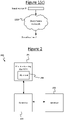
- Figure 1(a) gives a simplified representation of an example neural network 108.
- the example neural network comprises multiple layers of nodes 104: an input layer 102i, one or more hidden layers 102h and an output layer 102o. In practice, there may be many nodes in each layer, but for simplicity only a few are illustrated. Each node is configured to generate an output by carrying out a function on the values input to that node.
- the inputs to one or more nodes form the input of the neural network, the outputs of some nodes form the inputs to other nodes, and the outputs of one or more nodes form the output of the network.
- a weight may define the connectivity between a node in a given layer and the nodes in the next layer of the neural network.
- a weight can take the form of a scalar or a probabilistic distribution. When the weights are defined by a distribution, as in a Bayesian model, the neural network can be fully probabilistic and captures the concept of uncertainty.
- the values of the connections 106 between nodes may also be modelled as distributions. This is illustrated schematically in Figure 1(b) .
- the distributions may be represented in the form of a set of samples or a set of parameters parameterizing the distribution (e.g. the mean ⁇ and standard deviation ⁇ or variance ⁇ 2 ).
- the network learns by operating on data input at the input layer, and, based on the input data, adjusting the weights applied by some or all of the nodes in the network.
- each node takes into account the back propagated error and produces a revised set of weights. In this way, the network can be trained to perform its desired operation.
- the input to the network is typically a vector, each element of the vector representing a different corresponding feature.
- the elements of this feature vector may represent different pixel values, or in a medical application the different features may represent different symptoms.
- the output of the network may be a scalar or a vector.
- the output may represent a classification, e.g. an indication of whether a certain object such as an elephant is recognized in the image, or a diagnosis of the patient in the medical example.
- Figure 1(c) shows a simple arrangement in which a neural network is arranged to predict a classification based on an input feature vector.
- experience data comprising a large number of input data points is supplied to the neural network, each data point comprising an example set of values for the feature vector, labelled with a respective corresponding value of the classification (e.g. elephant or not elephant).
- the learning algorithm tunes the weights to reduce the overall error in the network.
- a target feature vector can then be input to the neural network without a label, and the network can instead predict the value of the classification based on the input feature values and the tuned weights.
- Training in this manner is sometimes referred to as a supervised approach.
- Other approaches are also possible, such as a reinforcement approach wherein the network each data point is not initially labelled.
- the learning algorithm begins by guessing the corresponding output for each point, and is then told whether it was correct, gradually tuning the weights with each such piece of feedback.
- Another example is an unsupervised approach where input data points are not labelled at all and the learning algorithm is instead left to infer its own structure in the experience data.
- missing values in the data set can be predicted by machine learning methods This can be used to predict why certain values are missing in a data set, which provides a more accurate system for determining missing values in data sets input into the system by reducing bias introduced into a system by relationships between missing variables. This allows the system to predict missing values for input data where the data is missing not at random.
- a computer-implemented method of machine learning comprises receiving values of a plurality of features for each data point in a set of data, the set of data comprising at least one missing value of a feature for at least one data point.
- a first neural network having a first set of parameters is used to encode the set of data into a first plurality of latent vectors.
- a second neural network having a second set of parameters is used to decode the plurality of latent vectors into a computed vector for each data point.
- the method comprises inputting the computed vector for each data point into a third neural network having a third set of parameters to determine a computed set of mask vectors comprising a computed mask vector for each data point, wherein each computed mask vector comprises a computed binary value for each feature to indicate whether a value for each feature is missing or not.
- the method also comprises using a fourth neural network having a fourth set of parameters to encode background data for each data point into a second plurality of latent vectors.
- the method comprises tuning the first, second and third set of parameters by minimising a loss function, the loss function comprising a sum of: a measure of difference between the first plurality of latent vectors and the second plurality of latent vectors; and an error determined based on the set of computed vectors, the set of computed mask vectors and ground truth data for the set of data.
- a loss function comprising a sum of: a measure of difference between the first plurality of latent vectors and the second plurality of latent vectors; and an error determined based on the set of computed vectors, the set of computed mask vectors and ground truth data for the set of data.
- the values of the variables of the input vector may not be fully observed, because the values for certain features are not observed. This is common in real world scenarios where a value may not be obtained for each variable of an input vector. All missing data problems fall into one of the following three categories: Missing Completely At Random (MCAR), Missing At Random (MAR), and Missing Not At Random (MNAR). Data are MCAR if the cause of missingness is purely random, e.g., some entries are deleted due to a random computer error. Data are MAR when the direct cause of missingness is fully observed. For example, a dataset consists of two variables: gender and income, where gender is always observed and income has missing entries.
- MAR missingness would occur when men are more reluctant than women to disclose their income (i.e., gender causes missingness). Data that are neither MAR nor MCAR fall under the MNAR category. In the example above, MNAR would occur when gender also has missing entries. MNAR is the most common case and most challenging to solve technically. Our solution can handle all these different missingness patterns.
- the following will present a method of machine learning.
- the method tunes weights of neural networks in a system based on training data.
- the tuned neural networks can be used to impute missing values in input data sets.
- Some examples take into account a Missing Not At Random (MNAR) relationship between recorded values to improve accuracy of missing value imputation when data are MNAR.
- MNAR Missing Not At Random
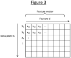
- FIG. 2 illustrates an example computing apparatus 200 for implementing an artificial intelligence (AI) algorithm including a machine-learning model in accordance with embodiments described herein.
- the computing apparatus 200 may take the form of a user terminal such as a desktop computer, laptop computer, tablet, smartphone, wearable smart device such as a smart watch, an on-board computer of a vehicle such as car, or a managing computing system for a set of sensors etc. Additionally or alternatively, the computing apparatus 200 may comprise a server.
- a server herein refers to a logical entity which may comprise one or more physical server units located at one or more geographic sites. Where required, distributed or "cloud" computing techniques are in themselves known in the art.
- the one or more user terminals and/or the one or more server units of the server may be connected to one another via a packet-switched network, which may comprise for example a wide-area internetwork such as the Internet, a mobile cellular network such as a 3GPP network, a wired local area network (LAN) such as an Ethernet network, or a wireless LAN such as a Wi-Fi, Thread or 6LoWPAN network.
- a packet-switched network may comprise for example a wide-area internetwork such as the Internet, a mobile cellular network such as a 3GPP network, a wired local area network (LAN) such as an Ethernet network, or a wireless LAN such as a Wi-Fi, Thread or 6LoWPAN network.
- the computing apparatus 200 comprises at least a controller 202, an interface (e.g., a user interface) 204, and an artificial intelligence (AI) algorithm 206.
- the controller 202 is operatively coupled to each of the interface 204 and the AI algorithm 206.
- Each of the controller 202, interface 204 and AI algorithm 206 may be implemented in the form of software code embodied on computer readable storage and run on processing apparatus comprising one or more processors such as CPUs, work accelerator co-processors such as GPUs, and/or other application specific processors, implemented on one or more computer terminals or units at one or more geographic sites.
- the storage on which the code is stored may comprise one or more memory devices employing one or more memory media (e.g. electronic or magnetic media), again implemented on one or more computer terminals or units at one or more geographic sites.
- one, some or all the controller 202, interface 204 and AI algorithm 206 may be implemented on the server.
- a respective instance of one, some or all of these components may be implemented in part or even wholly on each of one, some or all of the one or more user terminals.
- the functionality of the above-mentioned components may be split between any combination of the user terminals and the server.
- distributed computing techniques are in themselves known in the art. It is also not excluded that one or more of these components may be implemented in dedicated hardware.
- the controller 202 comprises a control function for coordinating the functionality of the interface 204 and the AI algorithm 206.
- the interface 204 refers to the functionality for receiving and/or outputting data.
- the interface 204 may comprise a user interface (UI) for receiving and/or outputting data to and/or from one or more users, respectively; or it may comprise an interface to a UI on another, external device.
- the interface may be arranged to collect data from and/or output data to an automated function implemented on the same apparatus or an external device.
- the interface 204 may comprise a wired or wireless interface for communicating, via a wired or wireless connection respectively, with the external device.
- the interface 204 may comprise one or more constituent types of interface, such as voice interface, and/or a graphical user interface.
- the interface 204 may present a UI front end to the user(s) through one or more I/O modules on their respective user device(s), e.g., speaker and microphone, touch screen, etc., depending on the type of user interface.
- the logic of the interface may be implemented on a server and output to the user through the I/O module(s) on his/her user device(s). Alternatively, some or all of the logic of the interface 204 may also be implemented on the user device(s) 102 its/themselves.
- the controller 202 is configured to control the AI algorithm 206 to perform operations in accordance with the embodiments described herein. It will be understood that any of the operations disclosed herein may be performed by the AI algorithm 206, under control of the controller 202 to collect experience data from the user and/or an automated process via the interface 204, pass it to the AI algorithm 206, receive predictions back from the AI algorithm and output the predictions to the user and/or automated process through the interface 204.
- the AI algorithm 206 comprises a machine-learning model 208, comprising one or more constituent statistical models such as one or more neural networks.
- FIG. 1(a) illustrates the principle behind a neural network.
- a neural network 100 comprises a graph of interconnected nodes 104 and edges 106 connecting between nodes, all implemented in software.
- Each node 104 has one or more input edges and one or more output edges.
- the input edges of one or more of the nodes 104 form the overall input 108i to the graph (typically an input vector, i.e., there are multiple input edges).
- the output edges of one or more of the nodes 104 form the overall output 108o of the graph (which may be an output vector in the case where there are multiple output edges). Further, the output edges of at least some of the nodes 104 form the input edges of at least some others of the nodes 104.
- Each node 104 represents a function of the input value(s) received on its input edges(s) 106i, the outputs of the function being output on the output edge(s) 106o of the respective node 104, such that the value(s) output on the output edge(s) 106o of the node 104 depend on the respective input value(s) according to the respective function.
- the function of each node 104 is also parametrized by one or more respective parameters w, sometimes also referred to as weights (not necessarily weights in the sense of multiplicative weights, though that is certainly one possibility).
- weights not necessarily weights in the sense of multiplicative weights, though that is certainly one possibility.
- Each weight could simply be a scalar value.
- the respective weight may be modelled as a probabilistic distribution such as a Gaussian.
- the neural network 100 is sometimes referred to as a Bayesian neural network.
- the value input/output on each of some or all of the edges 106 may each also be modelled as a respective probabilistic distribution.
- the distribution may be modelled in terms of a set of samples of the distribution, or a set of parameters parameterizing the respective distribution, e.g., a pair of parameters specifying its centre point and width (e.g. in terms of its mean ⁇ and standard deviation ⁇ or variance ⁇ 2 ).
- the nodes 104 of the neural network 100 may be arranged into a plurality of layers, each layer comprising one or more nodes 104.
- the neural network 100 comprises an input layer 102i comprising one or more input nodes 104i, one or more hidden layers 102h (also referred to as inner layers) each comprising one or more hidden nodes 104h (or inner nodes), and an output layer 102o comprising one or more output nodes 104o.
- hidden layers 102h also referred to as inner layers
- output layer 102o comprising one or more output nodes 104o.
- the different weights of the various nodes 104 in the neural network 100 can be gradually tuned based on a set of experience data (e.g., training data), so as to tend towards a state where the output 108o of the network will produce a desired value for a given input 108i.
- the neural network 100 may first be trained for that application. Training comprises inputting experience data in the form of training data to the inputs 108i of the graph and then tuning the weights w of the nodes 104 based on feedback from the output(s) 108o of the graph.
- the training data comprises multiple different input data points, each comprising a value or vector of values corresponding to the input edge or edges 108i of the graph 100.
- training data may comprise a set of ground truth data.
- the training data may comprise ground truth data with some of the data removed.
- each element of the feature vector X may represent a respective pixel value. For instance, one element represents the red channel for pixel (0,0); another element represents the green channel for pixel (0,0); another element represents the blue channel of pixel (0,0); another element represents the red channel of pixel (0,1); and so forth.
- each of the elements of the feature vector may represent a value of a different symptom of the subject, or physical feature of the subject or other fact about the subject (e.g. body temperature, blood pressure, etc.).
- Each data point n comprises a respective set of values of the feature vector (where x nd is the value of the d th feature in the n th data point).
- the input feature vector X n represents the input observations for a given data point, where in general any given observation i may or may not comprise a complete set of values for all the elements of the feature vector X.
- the neural network 100 can then be used to infer a value of the output 108o for a given value of the input vector 108i (X), or vice versa.
- Explicit training based on labelled training data is sometimes referred to as a supervised approach.
- Other approaches to machine learning are also possible.
- the AI algorithm 206 receives feedback (e.g., from a human) as to whether the prediction was correct, and uses this to tune the weights so as to perform better next time.
- feedback e.g., from a human
- the AI algorithm receives no labelling or feedback and instead is left to infer its own structure in the experienced input data.
- Figure 1A is a simple example of the use of a neural network 100.
- the machine-learning model 208 may comprise a structure of two or more constituent neural networks 100.
- Figure 4 schematically illustrates one such example, known as a variational auto encoder (VAE).
- the machine learning model 208 comprises an encoder 208q comprising at least one inference network, and a decoder 208p comprising one or more generative networks.
- Figure 4 is shown to give context of how a latent vector may be determined.
- Each of the inference networks and the generative networks is an instance of a neural network 100, such as discussed in relation to Figure 1(a) .
- An inference network for the present purposes means a neural network arranged to encode an input into a latent representation of that input, and a generative network means a network arranged to at least partially decode from a latent representation.
- the one or more inference networks are arranged to receive the observed feature vector X as an input and encode it into a latent vector Z (a representation in a latent space).
- the one or more generative networks 208p are arranged to receive the latent vector Z and decode back to the original feature space X.
- the latent vector Z is a compressed (i.e. encoded) representation of the information contained in the input observations X.
- a VAE no one element of the latent vector Z necessarily represents directly any real world quantity, but the vector Z as a whole represents the information in the input data in compressed form.
- Z may be a probabilistic random vector.
- the encoder/inference network of a VAE is in some examples parameterized to encode the observed feature X into the statistics of Z (i.e., mean and variance).
- the encoder can be represented by q ⁇ (Z
- the decoder 404 is arranged to decode the latent vector Z back into values in a real-world feature space, i.e., back to an uncompressed form representing the actual observed properties (e.g. pixel values).
- the weights w of the one or more inference networks 208q are labelled herein ⁇ , whilst the weights w of the one or more generative networks 208p are labelled ⁇ .
- Each node 104 applies its own respective weight as illustrated in Figure 3 , but elsewhere herein the label ⁇ generally may be used to refer to a vector of weights in one or more of the inference networks 208q, and ⁇ to refer to a vector of weights in one or more of the generative networks 208p.
- the weights ⁇ and ⁇ are tuned so that the VAE 208 learns to encode the feature vector X into the latent space Z and back again. For instance, this may be done by minimizing a measure of divergence between q ⁇ (Z n
- the prior distribution may be a known distribution.
- ” means “given”.
- the model is trained to reconstruct X n and therefore maintains a distribution over X n .
- the value of X n is known, and at the "output side", the likelihood of X n under the output distribution of the model is evaluated.
- the input values of X are sampled from the input data distribution.
- the goal in a VAE of the algorithm 206 is to make p(X) close to the input data distribution.
- p(X, Z) may be referred to as the model of the decoder, whilst p(Z
- p(z) and q(z) may be referred to as priors. Examples discussed further below may comprise similar steps to those used in a VAE, but with further modifications.
- this may be done by minimizing the Kullback-Leibler (KL) divergence between q ⁇ (Z n
- KL Kullback-Leibler
- the minimization may be performed using an optimization function such as an ELBO (evidence lower bound) function, which uses cost function minimization based on gradient descent.
- ELBO emit lower bound
- This is the general principle of an autoencoder.
- the latent vector Z is subject to an additional constraint that it follows a predetermined form (type) of probabilistic distribution such as a multidimensional Gaussian distribution or gamma distribution.
- Missing data is an obstacle in many data analysis problems, which may compromise the performance of machine learning models, as well as downstream tasks based on these models. Being able to successfully recover/impute missing data in an unbiased way is useful to understanding the structure of real-world data. In some examples, this is performed by identifying the underlying data-generating process. Further, in some examples this is performed by identifying probabilistic mechanism that decides which data is missing.
- the first type is missing completely at random (MCAR), where the probability of a data entry being missing is independent of both the observed and unobserved data. See for example, Figure 5(a) . In this case, no statistical bias is introduced by MCAR.
- the second type of missing mechanism is missing at random (MAR), which assumes that the missing data mechanism is independent of the value of unobserved data. See for example, Figure 5 (b) . Under this assumption, maximum likelihood learning methods without explicit modelling of the missingness mechanism can be applied by marginalizing out the missing variables.
- MAR missing at random
- MCAR and MAR do not hold in many real-world applications, such as recommender systems, healthcare, and surveys.
- participants with financial difficulties are more likely to refuse to complete the survey about financial incomes.
- MNAR missing not at random
- the cause of the missingness can be unobserved.
- ignoring the missingness mechanism will result in biased imputation, which will jeopardize down-stream tasks.
- MNAR data may comprise MNAR data.
- MNAR data may comprise MNAR data.
- the likelihood of having a blood oxygen level recorded for a patient may increase when the patient also has a blood pressure level recorded, because both measurements may be taken at the same time during a period when a patient is ill.
- Sensor data for a system of sensors may also comprise MNAR data. For example, if a certain data point is missing sensor data from one sensor, the likelihood of another sensor missing data may be increased, because for example a power outage to part or whole of the set of sensors may have caused the sensors not to record data.
- Figure 5 shows examples of different kind of missing mechanisms between one or more latent variables Z, vectors X 1 and X 2 , and mask vectors R 1 and R 2 .
- latent variable Z it should be understood that there may be more or fewer (there may in some examples be no latent vector as shown in example (f)).
- vectors X 1 and X 2 there may be more or fewer vectors X n .
- mask vectors R 1 and R 2 there may be more or fewer mask vectors R n .
- Arrows represent a relationship between variables.
- the data is MCAR, as there are only relationships between: Z and X 1 ; and Z and X 2 .
- the data is MAR, as there are relationships between: Z and X 1 ; Z and X 2 ; and X 1 and R 2 .
- the data is MNAR, as there are relationships between: Z and X 1 ; Z and X 2 ; X 1 and R 1 ; and X 2 and R 2 .
- the data is MNAR, as there are relationships between Z and X 1 ; Z and X 2 ; X 1 and R 1 ; X 2 and R 2 ; X 1 and R 2 ; and X 2 and R 1 .
- the data is MNAR, as there are relationships between: Z and X 1 ; Z and X 2 , Z and R 1 ; Z and R 2 .
- the data is MNAR as there are relationships between: X 1 and R 1 ; X 2 and R 2 ; X 1 and R 2 ; X 2 and R 1 ; and X 1 and X 2 .
- the data is MNAR as there are relationships between: Z and X 1 ; Z and X 2 ; X 1 and R 2 ; X 2 and R 1 ; and X 1 and X 2 .
- the data is MNAR as there are relationships between Z and X 1 ; Z and X 2 ; X 1 and R 1 ; X 2 and R 2 ; X 1 and R 2 ; X 2 and R 1 ; X 1 and R 2 ; and X 2 and R 1 .
- the data is MNAR as there are relationships between Z and X 1 ; Z and X 2 ; X 1 and R 1 ; X 2 and R 2 ; X 1 and R 2 ; X 2 and R 1 ; X 1 and R 2 ; X 2 and R 1 ; and X 1 and X 2 .
- the data is MNAR as there are relationships between Z and X 1 ; Z and X 2 ; X 1 and R 1 ; X 2 and R 2 ; X 1 and R 2 ; X 2 and R 1 ; X 1 and R 2 ; X 2 and R 1 ; X 1 and X 2 ; and R 1 and R 2 .
- Figure 6 shows an example set of data 620.
- the data set 620 comprises a number of data points N and 5 different features. It should be understood that the specific values shown in data set 620 for specific data points and specific features are exemplary only. It should also be understood that there may be more or fewer features.
- U For each data point n, there is background data u n .
- the total group of u n makes up group U.
- U may be considered to be a set of data comprising a value for every feature d and for every data point n in the set U. As such, U may be considered to comprise fully observed data.
- For one or more of data points n of x n,d there are missing (unobserved) values, such as the value for x 2,4 628 for example. These are indicated by "?” in the example of Figure 6 .
- For one or more of data points n of x n,d there are observed values, such as the value for x 1,3 626 for example
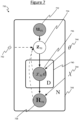
- Figure 7 shows an example of a model that can be used to impute missing values for MNAR data.
- a background data vector or value u n can be used to determine a prior p(z) of the latent vector z n . This can be performed over a set of N data points 748.
- the latent vectors determined by this method can be indicated as z n '.
- the prior p(Z) is only used in training and when performing imputation, both U and p(Z) are not used.
- the latent vectors z n ' may be determined based on u n using a relationship p(Z
- U) may be a distribution.
- the distribution may comprise a mean and variance determined by a neural network that takes U as an input.
- the distribution may be a Gaussian, but in other examples other distributions may be used.
- a latent vector z n can also be determined using a neural network having parameters ⁇ 742, values x n,d 736 and mask vector R n 738. This can be performed over D features 740 and N data points 742.
- the prior (Z n ') is used to regularize the encoder output/approximate posterior, q(Z n
- a neural network having parameters ⁇ is used to determine the encoded distribution q ⁇ (Z
- Monte Carlo sample z may give different values each time the sample is taken.
- Latent vector Z n (or z n ') 734 can be used to determine a computed value for variable x n,d 736 using a neural network having parameters ⁇ 744. This can be performed over D features 740 and N data points 748.
- Values x n,d 736 can be used to determine a mask vector R n 738 using a neural network having parameters ⁇ 746. This can be determined from the computed values of x n,d 736 determined as in the paragraph above. This can be performed over D features 740 and N data points 748.
- mask vector R n can also be determined based on a set of data values such input into the system, by determining which values are missing and using this to infer a mask vector R n .
- Figure 8 shows an example of how a system 830 for imputing missing values from MNAR data can be set up. This could be used to train the system of Figure 7 , for example.
- These x o values or vectors can comprise the observed data over feature vectors d and data points n.
- these x o values may be measured by a system or user and the missing values may naturally have occurred.
- the missing values can be artificially created by removing one or more values from a ground truth set of data 850. For example, for a certain feature d and/or for a certain data point n, values outside of a certain range or above a certain limit may be removed. For example, for a certain feature d, all values above a certain threshold may be removed to create missing data values in a data set.
- all values above a certain threshold may be removed to create missing data values in a data set.
- all values above a first threshold but below a second threshold may be removed to create missing data values in a data set.
- a first neural network 842 using a first set of parameters ⁇ encodes the x o values/vectors 836a and related R mask vectors 838a into one or more latent vectors Z 834.
- NN 842 determines q ⁇ (Z
- a fourth neural network 852 encodes a set of background data U 832, having fully observed data over all data points N (i.e., data with no missing values) to one or more latent vectors Z' 834a.
- the fourth neural network may use a set of parameters ⁇ . These parameters may be randomly generated. In some examples, these parameters may have been optimised prior to optimising ⁇ , ⁇ , ⁇ . In some examples, ⁇ may be further optimised along with ⁇ , ⁇ , ⁇ by minimising a loss function as described below. When the model is tuned correctly, the difference between Z 834 and Z'834a should be minimised.
- a measure of difference between Z and Z' is shown at 856. The measure of difference is dependent on the set of parameters ⁇ . In this example, Kullback-Leibler divergence of distributions q ⁇ (Z
- a second neural network 844 having a second set of parameters ⁇ is used to decode one or more random samples z ⁇ q ⁇ (Z
- calculated unobserved values x u ⁇ may also be determined.
- a third neural network 846 having a third set of parameters ⁇ is used to determine a plurality of computed mask vectors R 838b.
- the computed mask vectors comprise a binary value for each feature to indicate whether a value for each feature is determined to be missing or not.
- R is determined by p(R
- X,Z) may be a distribution whose mean parameter is determined by a neural network that takes X and Z as input.
- the distribution may be a Bernoulli distribution in some examples.
- the computed observed values x o ⁇ 836b and computed mask vectors R 838b are compared with ground truth data 850.
- this ground truth data 850 may have been used to generate R 838a and X o 836a.
- the ground truth data 850 may be a separate set of data which is known or assumed to be correct.
- the computed observed values x o ⁇ 836b and computed mask vectors R 838b are compared with ground truth data 850 to determine an error introduced by the first, second and third neural networks.
- the error may be determined using a mean squared difference, or any other suitable method for determining error between values.
- the error value 858 is dependent on ⁇ , ⁇ and ⁇ .
- the error may be determined using maximum likelihood learning (ML), where we use Gaussian likelihoods for X (which is equivalent to minimizing mean squared difference), and Bernoulli likelihood for R (which is equivalent to binary cross entropy loss).
- ML maximum likelihood learning
- the error may be determined using a function of the L2 norm as the error f x o ⁇ ⁇ x o 2 .
- a loss function 854 may be determined by a combination of the measure of difference 856 between distributions of Z and Z' determined respectively at 842 and 852 and the error value 858.
- the combination may comprise a sum of the measure of difference between Z and Z' 856 and the error value 858.
- a weighting factor may be applied to either of the measure of difference between Z and Z' 856 and the error value 858 before they are summed together.
- the parameters ⁇ , ⁇ and ⁇ of the first, second and third neural networks 842, 844 and 846 respectively can be varied in order to minimise the loss function 854.
- a gradient descent algorithm is used to tune (change) parameters ⁇ , ⁇ and ⁇ in order to minimise loss function 854.
- minimising the loss function a system that produces results similar to ground truth data 850 and that are linked to background data U is provided. This can be used to take into account any relationships between parameters of MNAR data.
- latent vectors Z 834 can also be used to determine mask vectors R 838b by inputting latent vectors Z 834 into neural network 3 846 as shown at 849.
- Figure 9 shows an example of a system 930 that can be used to impute missing values in a set of data.
- the system 930 may have been trained and the parameters tuned according to the method described above with respect to system 830.
- System 930 may be based on system 730 in some examples.
- the parameters ⁇ and ⁇ may have been set or temporarily set following the training method of Figure 8 .
- a set of observed values x o 936a is input into a first neural network 942 having parameters ⁇ to encode the observed values x o 936a into a latent vector Z 934. Encoding observed values x o 936a into a latent vector Z 934 can be done in two steps. First, neural network 842 determines q ⁇ (Z
- Mask vector R 938a may also be input into first neural network 942 with observed values x o 936a to indicate to first neural network 942 which values are unobserved in the input set of data. In some examples, mask vector R 938a and observed values x o 936a may be inferred from an input set of data by determining which variables are missing from the input set of data.
- the random sample of latent vector Z 934 can be decoded by second neural network 944 having parameters ⁇ to decode one or more latent vectors Z to output expected observed values x o ⁇ and expected x U ⁇ values 936c for the values that were unobserved in the input set of data.
- second neural network 944 having parameters ⁇ to decode one or more latent vectors Z to output expected observed values x o ⁇ and expected x U ⁇ values 936c for the values that were unobserved in the input set of data.
- expected observed values x o ⁇ and expected x U ⁇ values 936c may be output.
- These expected x U ⁇ values 936c can be used to fill in gaps in the set of data to provide a full set of imputed data.
- the information from the values included in the training data in Figure 8 is taken into account when imputing missing values, as well as the ground truth data 850 and the background data 832 used to train the data in Figure 8 .
- This system can then be used to predict values for missing values in other sets of data.
- the above-mentioned systems may be used to train a machine learning model for imputing values of MNAR data.
- the MNAR data may comprise one or more sensor values.
- Sensor data of one or more sensors that is missing from a data set may be imputed using the methods described above.
- the system for imputing the missing values may be tuned as described above.
- estimates of unobserved values can be provided. This can be used to diagnose faults with one or more systems measured by the sensors. In other examples, this can be used to detect changes in the state of an environment measured by the sensors.
- the sensors may be used to measure one or more devices.
- the imputed data can be used to diagnose faults with the one or more devices.
- the one or more devices may be located in a vehicle, for example.
- the background data U may comprise a location in of a sensor in a system being measured by the sensors.
- the background data may include a time of day for which each data point was recorded.
- the features of the data set that are imputed may comprise one or more of: temperature; air pressure; light conditions; levels of one or more chemicals in the atmosphere.
- the MNAR data may comprise values used in healthcare.
- Healthcare data that is missing from a healthcare data set may be imputed using the methods described above.
- the system for imputing the missing values may be tuned as described above.
- estimates of unobserved values can be provided. This can be used to diagnose patients monitored by the healthcare system.
- the background data U may comprise a gender of each patient.
- the background data may include an age for each patient.
- the features of the data set that are imputed may comprise one or more of: blood sugar; blood oxygen; body temperature of one or more body parts; heart rate; a diagnosis of a health condition, such as diabetes or anaemia for example.
- data values may be MNAR. If a patient has a blood oxygen measurement recorded, they may also have a blood sugar level and diabetes diagnosis recorded as these measurements may have been made simultaneously during a hospital visit. Further, each of these measurements may be indirectly related to age and gender background data U, as these variables may have an indirect effect of a likelihood of a visit to a hospital. By taking into account the background data U as described above, the links between the MNAR data can be determined, which helps to account for biases in the data set and therefore provide more accurate diagnosis based on input data comprising missing values.
- a system for imputing data can be accurately tuned taking into account reasons for a missingness MNAR mechanism in data. This provides more accurate subsequent decisions based on imputed values in data sets input into the model.
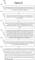
- Figure 12 shows an example method 1200. The method may be performed by a computing device or over one or more computing devices.
- the method comprises receiving values of a plurality of features for each data point in a set of data, the set of data comprising at least one missing value of a feature for at least one data point.
- the method comprises using a first neural network having a first set of parameters to encode the set of data into a distribution of a first plurality of latent vectors.
- the method comprises using a second neural network having a second set of parameters to decode a random sample of the distribution of the first plurality of latent vectors into a computed vector for each data point.
- the method comprises inputting the computed vector for each data point into a third neural network having a third set of parameters to determine a computed set of mask vectors comprising a computed mask vector for each data point, wherein each computed mask vector comprises a computed binary value for each feature to indicate whether a value for each feature is missing or not.
- the method comprises using a fourth neural network having a fourth set of parameters to encode background data for each data point into a distribution of a second plurality of latent vectors.
- the method comprises tuning the first, second and third set of parameters by minimising a loss function, the loss function comprising a sum of: a measure of difference between the distribution of the first plurality of latent vectors and the distribution of the second plurality of latent vectors; and an error determined based on the set of computed vectors, the set of computed mask vectors and ground truth data for the set of data.
- the loss function comprising a sum of: a measure of difference between the distribution of the first plurality of latent vectors and the distribution of the second plurality of latent vectors; and an error determined based on the set of computed vectors, the set of computed mask vectors and ground truth data for the set of data.
- Model Identifiability is useful for analyzing model behaviour under missing data.
- We give the definition below [see e.g. Dawen Liang, Laurent Charlin, James Mclnerney, and David M Blei. Modeling user exposure in recommendation. In Proceedings of the 25th international conference on World Wide Web, pages 951-961, 2016 and also Thomas J Rothenberg. Identification in parametric models. Econometrica: Journal of the Econometric Society, pages 577-591, 1971 ]:
- a model pe(X) is identifiable, if different parameter configurations implies a different probabilistic distributions over the observed variables. With identifiability guarantee, if the model assumption is correct, the true generation process can be recovered. Next, we introduce necessary notations and of missing data, and set up a concrete problem setting.
- p(X) on X the reference distribution that is, the distribution that we would have observed if no missing mechanism is present; and we call the conditional distribution p(R
- X is the cause of R, and the connections between X and R are fully connected, i.e., each single node in R are caused by the entire set X. All nodes in R are conditionally independent from each other given X.
- Rubin proposed to jointly optimize both the reference distribution p ⁇ (X) and the missing data mechanism p ⁇ (R
- Definition 2.1 One key issue of training probabilistic models under MNAR missing data is its identifiability. Recall that (Definition 2.1) model identifiability characterize the property that the mapping from parameter ⁇ to the distribution p ⁇ (X) is one-to-one. This is often closely related to maximum likelihood learning. In fact, it is not hard to show that Definition 2.1 is equivalent to the following Definition 3.1:
- the "correct" model parameter ⁇ * can be identified via maximum likelihood learning (under complete data), and the ML solution is unbiased.
- MNAR missing mechanism we perform maximum likelihood learning on both X o and R using Eq. 1.
- log p ⁇ , ⁇ (X o ,R) we need log p ⁇ , ⁇ (X o ,R) to be identifiable under MNAR, so that we can correctly identify the ground truth data generating process, and achieve unbiased imputation.
- the identifiability of log p ⁇ , ⁇ (X o ,R) under MNAR is usually not guaranteed, even in some simplistic settings [ Wang Miao, Peng Ding, and Zhi Geng. Identifiability of normal and normal mixture models with nonignorable missing data. Journal of the American Statistical Association, 111(516):1673-1683, 2016 ]. In this section, we will give the sufficient conditions for model identifiability under MNAR, and study how these can be relaxed for real-world applications.
- Each ⁇ is the parameter that parameterizes the conditional distribution that connects X d and Z, p ⁇ d ( X d
- the ground truth parameter of p D belongs to the model parameter space, ( ⁇ *, ⁇ *) ⁇ ⁇ .
- our goal is to correctly identify the ground truth parameter settings given partially observed samples from p D (X o ,X u , R).
- Subset identifiability There exist a partition (which may be arbitrary in the set theory sense) of I, denoted by A I ⁇ O s ⁇ 1 ⁇ s ⁇ S , such that: for all O s ⁇ A I , p ⁇ (X Os ) responsible for the identifiability on a subset of parameters.
- This assumption is about the strict positivity of the ground truth data generating process, p D (Xo,Xu,R).
- A1 ensures that our model has the same graphical representation/parametric forms as the ground truth;
- Assumption A3 ensures that p D (X o ,X u , R) should be positive for certain important patterns (i.e., those on which p(Xo) is identifiable). Given these assumptions, we have the following proposition (See Appendix C for proof.):
- Proposition 1 (Sufficient conditions for identifiability under MNAR). Let p ⁇ , ⁇ (X o , X u , R) be a model on the observable variables X, and missing pattern R, and p D (X o ,X u , R) be the ground truth distribution. Assume that they satisfies Data setting D1, Assumptions A1, A2 and A3.
- Missing value imputation as inference Given a model p ( ⁇ ) (X o , X u ), the missing data imputation problem can be then formularized by the Bayesian inference problem p ⁇ (X u
- Proposition 1 can be extended to the case where model identifiability is defined by equivalence classes. See Appendix F for details.
- ⁇ is a subset of ⁇ on which ⁇ is defined.
- p ⁇ ⁇ , ⁇ X o X u R p ⁇ ⁇ 1 ⁇ ⁇ X o X u R
- ⁇ ⁇ R I be the parameter domain of the model p ⁇ , ⁇ ( X o , X u , R ).
- mapping ⁇ ⁇ ⁇ ⁇ ⁇ ⁇ ⁇ R I ⁇ ⁇ ⁇ ⁇ ⁇ R J is one-to-one on ⁇ (equivalently, the inverse mapping ⁇ -1 : ⁇ ⁇ ⁇ is injective, and ⁇ is its image set).
- p ⁇ ⁇ , ⁇ ( X o , R ⁇ ) p ⁇ -1 ( ⁇ , ⁇ ) ( X o , R ).
- p ⁇ is identifiable w.r.t. ( ⁇ , ⁇ ), if p ⁇ , ⁇ ( X o , R ) is identifiable w.r.t. ⁇ and ⁇ .
- Equation 3 i.e., Assumption A1; and 2
- Proposition 3 (Sufficient conditions for identifiability under MNAR and data-model mismatch).
- p ⁇ , ⁇ ( X o , X u , R) be a model on the observable variables X and missing pattern R
- p D (X o ,X u , R) be the ground truth distribution. Assume that they satisfies Data setting D2, Assumption A2, A3, and A4.
- Proposition 3 allows us to deal with the cases where the parameterization of ground truth data generating process and model distribution are related through a set of mappings, ⁇ ⁇ o ⁇ .
- the graphical structure of p D (X o ,X u , R) can be any cases in Figure 5 excluding (j). Then, in those cases, we are still able to use a model that corresponds to Equation 3 ( Fig 5 (h) ) to perform ML learning, provided that our model is flexible enough (Assumption A4). This greatly improves the applicability of our identifiability results, and we can build a practical algorithm based on Equation 3 to handle many practical MNAR cases.
- GINA a deep generative imputation model for MNAR data ( Figure 2 ). GINA fulfils identifiability assumptions above, and can handle general MNAR case.
- the parametric form of GINA We use utilize the flexibility of deep generative models to model the data generating process.
- the reference model p ⁇ ( X ) is parameterized by an identifiable VAE to satisfy Assumption A2. That is, p ⁇ ( X
- U ) ⁇ Z dZp ⁇ (X - f ( Z )) p ( Z
- the decoder p ⁇ ( X - f ⁇ ( Z )) is parameterized by a neural network, f : R H ⁇ R D .
- Equation 1 the joint likelihood in Equation 1 is intractable.
- X o ) the joint likelihood in Equation 1 is intractable.
- X o ) the joint likelihood in Equation 1 is intractable.
- arXiv preprint arXiv:1808.06581, 2018 also Dawen Liang, Laurent Charlin, and David M Blei. Causal inference for recommendation ]. Similar to the use of the missing model, they have used an explicit model of exposure and adopted a causal view, where MNAR is treated as a confounding bias. Apart from these, inverse probability weighting methods are also used to debias the effect of MNAR [ Tobias Schnabel, Adith Swaminathan, Ashudeep Singh, Navin Chandak, and Thorsten Joachims. Recommendations as treatments: Debiasing learning and evaluation.
- arXiv preprint arXiv:1602.05352, 2016 also Xiaojie Wang, Rui Zhang, Yu Sun, and Jianzhong Qi. Doubly robust joint learning for recommendation on data missing not at random.
- PMLR International Conference on Machine Learning, pages 6638-6647. PMLR, 2019 , also Wei Ma and George H Chen. Missing not at random in matrix completion: The effectiveness of estimating missingness probabilities under a low nuclear norm assumption.
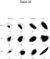
- Figure 10 shows a Visualization of generated X2 and X3 from synthetic experiment.
- Contour plot kernel density estimate of ground truth density of complete data.
- Table 2 Performance on Eedi education dataset (with standard errors) Method Debiased MSE Level change (correct) Level change (incorrect) p-value PVAE 0.194 ⁇ 0.001 0.131 ⁇ 0.138 -0.101 ⁇ 0.160 0.514 Not-MIWAE 0.192 ⁇ 0.000 0.062 ⁇ 0.142 -0.073 ⁇ 0179 0.561 GINA 0.188 ⁇ 0.001 0.945 ⁇ 0.151 -0.353 ⁇ 0.189 1.01 ⁇ 10 -7
- CCA complete case analysis
- imputation based methods such as listwise deletion [ Paul D Allison. Missing data. Sage publications, 2001 ] and pairwise deletion [ HerbertWMarsh. Pairwise deletion for missing data in structural equation models: Nonpositive definite matrices, parameter estimates, goodness of fit, and adjusted sample sizes.
- Listwise/pairwise deletion methods are known to be unbiased under MCAR, and will be biased under MAR/MNAR.
- imputation based methods tries to replace missing values by imputed/predicted values.
- One popular imputation technique is called single imputation, where only produce one single set of imputed values for each data instance.
- Standard techniques of single imputation include mean/zero imputation, regression-based imputation [ Paul D Allison. Missing data. Sage publications, 2001 ], no-parametric methods [ Phimmarin Keerin, Werasak Kurutach, and Tossapon Boongoen. Cluster-based knn missing value imputation for dna microarray data. In 2012 IEEE International Conference on Systems Man, and Cybernetics (SMC), pages 445-450. IEEE, 2012 ].
- MI multiple imputation
- arXiv preprint arXiv:2006.12871, 2020 a VAE model for MNAR data trained by jointly maximizing the likelihood on both the partially observed data and the missing pattern.
- the latent priors p(Z) for both PVAE and Not-MIWAE are parameterized by a standard normal distribution, hence no auxiliary variables are used.
- the graphical model of Not-MIWAE is described by Fig 5 (a) , and does not handle the scenarios where the ground truth data distribution follows other graphs like Fig 5 (g) .
- the inference model q(ZjX) for the underlying VAEs is set to be diagonal Gaussian distributions whose mean and variance are parameterized by neural nets as in standard VAEs [ Diederik P Kingma and Max Welling. Auto-encoding variational bayes. arXiv preprint arXiv:1312.6114, 2013 ] (with missing values replaced by zeros[ Alfredo Nazabal, Pablo M Olmos, Zoubin Ghahramani, and Isabel Valera. Handling incomplete heterogeneous data using vaes.
- h w is a linear mapping with coefficients w
- f is some non-linear mapping whose functional form is given by Appendix B
- ⁇ 1 & ⁇ 2 are two different sets of parameters for f
- ⁇ 1 , ⁇ 2 , ⁇ 3 are observational noise variables with mean 0, variance 0.01.
- arXiv preprint arXiv:1809.11142, 2018 ] we use 20 dimensional feature mapping h parameterized by a single layer neural network and 20 dimensional ID vectors for each variable.
- the symmetric operator is set to be the summation operator.
- Eedi dataset is a binary matrix with 1/0 indicating that the student response is correct/incorrect
- decoder p_(XjZ) uses a 50-20-50-D structure. Such structure is chosen using the validation set using grid search.
- ReLU activation function for the decoder (except for output layer, where no activation function is used).
- inference net we use the point net structure that were used in Yahoo!R3 dataset.
- the difference is that we use 50 dimensional feature mapping h parameterized by a single layer neural network and 10 dimensional ID vectors for each variable. All methods are trained with 1k epochs with batchsize 100.
- X), by multiplying a factor of ⁇ 0:5. This is due to that majority of the student response matrix is missing, the p ⁇ (R
- ⁇ be a equivalence relation on a parameter space ⁇ . That is, it satisfies reflexivity ( ⁇ 1 ⁇ ⁇ 2 ), symmetry (( ⁇ 1 ⁇ ⁇ 2 ) if and only if ( ⁇ 2 ⁇ ⁇ 1 ), and transitivity (if ⁇ 1 ⁇ ⁇ 2 and ⁇ 2 ⁇ ⁇ 3 , then ⁇ 1 ⁇ ⁇ 3 ).
- Definition F.1 Model identifiability based on equivalence relation.
- p ⁇ (X) is a distribution of some random variable X
- ⁇ is its parameter that takes values in some parameter space ⁇ ⁇ , and sim some equivalence relation on ⁇ .
- the GINA model needs satisfy the requirement on model of Proposition 1 or 3, if we wish to use it to fit to the partially observed data and then perform (unbiased) missing data imputation.
- the key assumption that we need to verify is the local identifiability (Assumption A2).
- the A in the ⁇ A equivalence relation can be further reduced to a permutation matrix. That is, the model parameters can be identified, such that the latent variables differs up to a permutation. This is not inconsequential in many applications.
- X o be the set of observed variables, that represents the correctness of student's response to questions that are presented to them.
- O ⁇
- n (i) n (i) to O. This process is done by maximizing the information reward proposed by [ Chao Ma, Sebastian Tschiatschek, Konstantina Palla, Jose Miguel Hernandez-Lobato, Sebastian Nowozin, and Cheng Zhang.
- X ⁇ X U .
- X ⁇ could be ver high-dimensional, and direct estimation of KL[p(X ⁇
- each model are trained on the randomly generated, partially observed synthetic dataset described above. Once the models are trained, they are used to impute the missing data in the training set. For each training data, we draw exactly one sample from the (approximate) conditional distribution p t heta(X u
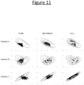
- Figure 11 shows a visualization of imputed X2 and X3 from synthetic experiment.
- a computer-implemented method comprising: receiving values of a plurality of features for each data point in a set of data, the set of data comprising at least one missing value of a feature for at least one data point; using a first neural network having a first set of parameters to encode the set of data into a distribution of a first plurality of latent vectors; using a second neural network having a second set of parameters to decode a random sample of the distribution of the first plurality of latent vectors into a computed vector for each data point; inputting the computed vector for each data point into a third neural network having a third set of parameters to determine a computed set of mask vectors comprising a computed mask vector for each data point, wherein each computed mask vector comprises a computed binary value for each feature to indicate whether a value for each feature is missing or not; using a fourth neural network having a fourth set of parameters to encode background data for each data point into a distribution of a
- the background data comprises fully observed data for one or more of the plurality of features of each data point.
- the set of data is determined by removing, from the ground truth data, values for one or more of the plurality of features outside of a range of values for each of the one or more features.
- the set of data comprises: one or more observed values for one or more of the data points; and a mask vector for each data point, where each mask vector comprises a binary value for each feature to indicate whether a value for each feature is missing or not.
- the mask vector for each data point in the set of data is inferred from the one or more observed values and the at least one missing value of a feature.
- the method comprises: setting the first and second set of parameters to tuned values to provide a tuned first set of parameters and a tuned second set of parameters; receiving a second set of data comprising at least one missing value of the features for at least one data point in the second set of data; using the first neural network having the tuned first set of parameters to encode the set of data into a distribution of a third plurality of latent vectors; sampling a random sample of latent vectors from the distribution of the third plurality of latent vectors; using the second neural network having the tuned second set of parameters to decode the random sample of latent vectors from the distribution of the third plurality of latent vectors to obtain the at least one missing value of the features for the at least one data point in the second set of data the background data is input by a user.
- the tuning the first, second and third set of parameters by minimising a loss function comprises using a gradient descent algorithm for each of the first, second and third set of parameters.
- the at least one missing value of a feature for at least one data point in the set of data comprises Missing Not At Random, MNAR, data.
- the set of data comprises one or more data values representing sensor values of one or more devices.
- the method is used to diagnose one or more malfunctions in the one or more devices.
- the set of data comprises one or more data values representing physical measurements of one or more patients.
- the method is used to diagnose the one or more patients.
- the background data comprises an age and a gender of each patient.
- a computer program embodied on computer-readable storage, the program comprising code configured so as when run on one or more processors to perform the operations of any preceding claim.
Landscapes
- Engineering & Computer Science (AREA)
- Physics & Mathematics (AREA)
- Theoretical Computer Science (AREA)
- General Health & Medical Sciences (AREA)
- Computing Systems (AREA)
- Biomedical Technology (AREA)
- Biophysics (AREA)
- Computational Linguistics (AREA)
- Data Mining & Analysis (AREA)
- Evolutionary Computation (AREA)
- Life Sciences & Earth Sciences (AREA)
- Molecular Biology (AREA)
- Artificial Intelligence (AREA)
- General Engineering & Computer Science (AREA)
- General Physics & Mathematics (AREA)
- Mathematical Physics (AREA)
- Software Systems (AREA)
- Health & Medical Sciences (AREA)
- Probability & Statistics with Applications (AREA)
- Image Analysis (AREA)
Priority Applications (4)
| Application Number | Priority Date | Filing Date | Title |
|---|---|---|---|
| EP21191394.2A EP4134871A1 (de) | 2021-08-13 | 2021-08-13 | Identifizierbare generative modelle für imputation von missing-not-at-random-daten |
| PCT/US2022/039665 WO2023018630A1 (en) | 2021-08-13 | 2022-08-08 | Identifiable generative models for missing not at random data imputation |
| US18/292,368 US20240403624A1 (en) | 2021-08-13 | 2022-08-08 | Identifiable generative models for missing not at random data imputation |
| EP22761033.4A EP4384944A1 (de) | 2021-08-13 | 2022-08-08 | Identifizierbare generative modelle für fehlende nicht bei zufälliger dateneinschreibung |
Applications Claiming Priority (1)
| Application Number | Priority Date | Filing Date | Title |
|---|---|---|---|
| EP21191394.2A EP4134871A1 (de) | 2021-08-13 | 2021-08-13 | Identifizierbare generative modelle für imputation von missing-not-at-random-daten |
Publications (1)
| Publication Number | Publication Date |
|---|---|
| EP4134871A1 true EP4134871A1 (de) | 2023-02-15 |
Family
ID=77338620
Family Applications (2)
| Application Number | Title | Priority Date | Filing Date |
|---|---|---|---|
| EP21191394.2A Withdrawn EP4134871A1 (de) | 2021-08-13 | 2021-08-13 | Identifizierbare generative modelle für imputation von missing-not-at-random-daten |
| EP22761033.4A Pending EP4384944A1 (de) | 2021-08-13 | 2022-08-08 | Identifizierbare generative modelle für fehlende nicht bei zufälliger dateneinschreibung |
Family Applications After (1)
| Application Number | Title | Priority Date | Filing Date |
|---|---|---|---|
| EP22761033.4A Pending EP4384944A1 (de) | 2021-08-13 | 2022-08-08 | Identifizierbare generative modelle für fehlende nicht bei zufälliger dateneinschreibung |
Country Status (3)
| Country | Link |
|---|---|
| US (1) | US20240403624A1 (de) |
| EP (2) | EP4134871A1 (de) |
| WO (1) | WO2023018630A1 (de) |
Cited By (3)
| Publication number | Priority date | Publication date | Assignee | Title |
|---|---|---|---|---|
| CN116662666A (zh) * | 2023-06-29 | 2023-08-29 | 联想(北京)有限公司 | 一种信息处理方法及装置 |
| CN117152578A (zh) * | 2023-10-31 | 2023-12-01 | 合肥工业大学 | 基于变分推断的不完整多视图数据预测方法及系统 |
| CN117556267A (zh) * | 2024-01-12 | 2024-02-13 | 闪捷信息科技有限公司 | 缺失样本数据填充方法、装置、存储介质和电子设备 |
Families Citing this family (4)
| Publication number | Priority date | Publication date | Assignee | Title |
|---|---|---|---|---|
| US20230259757A1 (en) * | 2022-02-16 | 2023-08-17 | Paypal, Inc. | Tiered input structures for machine learning models |
| US20240354844A1 (en) * | 2023-04-19 | 2024-10-24 | Truist Bank | Url-based data transmission systems and methods facilitating digital data form access |
| CN117892789B (zh) * | 2023-12-26 | 2024-08-13 | 北京大学 | 一种推荐系统预测模型的训练方法 |
| CN118585815B (zh) * | 2024-06-07 | 2025-04-15 | 青海师范大学 | 基于深度单纯形卷积神经网络的数据缺失插补方法及系统 |
Citations (1)
| Publication number | Priority date | Publication date | Assignee | Title |
|---|---|---|---|---|
| US20200372369A1 (en) * | 2019-05-22 | 2020-11-26 | Royal Bank Of Canada | System and method for machine learning architecture for partially-observed multimodal data |
-
2021
- 2021-08-13 EP EP21191394.2A patent/EP4134871A1/de not_active Withdrawn
-
2022
- 2022-08-08 US US18/292,368 patent/US20240403624A1/en active Pending
- 2022-08-08 EP EP22761033.4A patent/EP4384944A1/de active Pending
- 2022-08-08 WO PCT/US2022/039665 patent/WO2023018630A1/en not_active Ceased
Patent Citations (1)
| Publication number | Priority date | Publication date | Assignee | Title |
|---|---|---|---|---|
| US20200372369A1 (en) * | 2019-05-22 | 2020-11-26 | Royal Bank Of Canada | System and method for machine learning architecture for partially-observed multimodal data |
Non-Patent Citations (41)
| Title |
|---|
| ALFREDO NAZABAL, PABLO M OLMOS, ZOUBIN GHAHRAMANI, AND ISABEL VALERA: "Handling incomplete heterogeneous data using vaes", PATTERN RECOGNITION, vol. 107, 2020, pages 107501, XP086224591, DOI: 10.1016/j.patcog.2020.107501 |
| ANDRIY MNIHRUSS R SALAKHUTDINOV: "Probabilistic matrix factorization", ADVANCES IN NEURAL INFORMATION PROCESSING SYSTEMS, vol. 20, 2007, pages 1257 - 1264 |
| ARTHUR P DEMPSTERNAN M LAIRDDONALD B RUBIN: "Maximum likelihood from incomplete data via the em algorithm", JOURNAL OF THE ROYAL STATISTICAL SOCIETY: SERIES B (METHODOLOGICAL, vol. 39, no. 1, 1977, pages 1 - 22 |
| AUDE SPORTISSECLAIRE BOYERJULIE JOSSE: "Imputation and low-rank estimation with missing not at random data", STATISTICS AND COMPUTING, vol. 30, no. 6, 2020, pages 1629 - 1643, XP037258896, DOI: 10.1007/s11222-020-09963-5 |
| BENJAMIN M MARLINRICHARD S ZEMEL: "Collaborative prediction and ranking with nonrandom missing data", PROCEEDINGS OF THE THIRD ACM CONFERENCE ON RECOMMENDER SYSTEMS, 2009, pages 5 - 12, XP058401290, DOI: 10.1145/1639714.1639717 |
| CHAO MA, SEBASTIAN TSCHIATSCHEK, KONSTANTINA PALLA, JOSE MIGUEL HERNANDEZ-LOBATO, SEBASTIAN NOWOZIN, AND CHENG ZHANG.: "Eddi:Efficient dynamic discovery of high-value information with partial vae.", ARXIV:1809.11142, 2018 |
| CHAO MASEBASTIAN TSCHIATSCHEKKONSTANTINA PALLAJOSE MIGUEL HERNANDEZ-LOBATOSEBASTIAN NOWOZINCHENG ZHANG: "Eddi: Efficient dynamic discovery of high-value information with partial vae", ARXIV:1809.11142, 2018 |
| DAWEN LIANGLAURENT CHARLINDAVID M BLEI, CAUSAL INFERENCE FOR RECOMMENDATION |
| DAWEN LIANGLAURENT CHARLINJAMES MCLNERNEYDAVID M BLEI: "Modeling user exposure in recommendation", PROCEEDINGS OF THE 25TH INTERNATIONAL CONFERENCE ON WORLD WIDE WEB, 2016, pages 951 - 961, XP058080304, DOI: 10.1145/2872427.2883090 |
| DIEDERIK P KINGMAMAX WELLING: "Auto-encoding variational bayes", ARXIV:1312.6114, 2013 |
| DONALD B RUBIN: "Formalizing subjective notions about the effect of nonrespondents in sample surveys", JOURNAL OF THE AMERICAN STATISTICAL ASSOCIATION, vol. 72, no. 359, 1977, pages 538 - 543 |
| DONALD B RUBIN: "Inference and missing data", BIOMETRIKA, vol. 63, no. 3, 1976, pages 581 - 592 |
| DONALD B RUBIN: "Multiple imputation for nonresponse in surveys", vol. 81, 2004, JOHN WILEY & SONS |
| GRAZIANO MITA ET AL: "An Identifiable Double VAE For Disentangled Representations", ARXIV.ORG, CORNELL UNIVERSITY LIBRARY, 201 OLIN LIBRARY CORNELL UNIVERSITY ITHACA, NY 14853, 10 February 2021 (2021-02-10), XP081877098 * |
| GUANG LINGHAIQIN YANGMICHAEL R LYUIRWIN KING: "Response aware model-based collaborative filtering", ARXIV:1210.4869, 2012 |
| HERBERTWMARSH: "Pairwise deletion for missing data in structural equation models: Nonpositive definite matrices, parameter estimates, goodness of fit, and adjusted sample sizes", STRUCTURAL EQUATION MODELING: A MULTIDISCIPLINARY JOURNAL, vol. 5, no. 1, 1998, pages 22 - 36 |
| IAN R WHITEPATRICK ROYSTONANGELA M WOOD: "Multiple imputation using chained equations: issues and guidance for practice", STATISTICS IN MEDICINE, vol. 30, no. 4, 2011, pages 377 - 399 |
| ILYES KHEMAKHEMDIEDERIK KINGMARICARDO MONTIAAPO HYVARINEN: "Variational autoencoders and nonlinear ica: A unifying framework", INTERNATIONAL CONFERENCE ON ARTIFICIAL INTELLIGENCE AND STATISTICS, 2020, pages 2207 - 2217 |
| JAMES L ARBUCKLEGEORGE A MARCOULIDESRANDALL E SCHUMACKER: "Full information estimation in the presence of incomplete data", ADVANCED STRUCTURAL EQUATION MODELING: ISSUES AND TECHNIQUES, vol. 243, 1996, pages 277 |
| JAMES M ROBINSANDREA ROTNITZKYLUE PING ZHAO: "Estimation of regression coefficients when some regressors are not always observed", JOURNAL OF THE AMERICAN STATISTICAL ASSOCIATION, vol. 89, no. 427, 1994, pages 846 - 866 |
| JOSE MIGUEL HERNANDEZ-LOBATONEIL HOULSBYZOUBIN GHAHRAMANI: "Probabilistic matrix factorization with non-random missing data", INTERNATIONAL CONFERENCE ON MACHINE LEARNING, 2014, pages 1512 - 1520 |
| JOSEPH G IBRAHIMSTUART R LIPSITZM-H CHEN: "Missing covariates in generalized linear models when the missing data mechanism is non-ignorable", JOURNAL OF THE ROYAL STATISTICAL SOCIETY: SERIES B (STATISTICAL METHODOLOGY, vol. 61, no. 1, 1999, pages 173 - 190 |
| KARTHIKA MOHANJUDEA PEARLJIN TIAN: "Graphical models for inference with missing data", ADVANCES IN NEURAL INFORMATION PROCESSING SYSTEMS, vol. 26, 2013, pages 1277 - 1285 |
| NIELS BRUUN IPSENPIERRE-ALEXANDRE MATTEIJES FRELLSEN: "not-miwae: Deep generative modelling with missing not at random data", ARXIV:2006.12871, 2020 |
| NIELS BRUUN IPSENPIERRE-ALEXANDRE MATTEIJES FRELLSEN: "not-miwae:Deep generative modelling with missing not at random data.", ARXIV:2006.12871, 2020 |
| OLEG IVANOV ET AL: "Variational Autoencoder with Arbitrary Conditioning", ARXIV.ORG, CORNELL UNIVERSITY LIBRARY, 201 OLIN LIBRARY CORNELL UNIVERSITY ITHACA, NY 14853, 6 June 2018 (2018-06-06), XP081380176 * |
| PAUL D ALLISON: "Missing data", SAGE PUBLICATIONS, 2001 |
| PHIMMARIN KEERINWERASAK KURUTACHTOSSAPON BOONGOEN: "2012 IEEE International Conference on Systems Man, and Cybernetics (SMC", 2012, IEEE, article "Cluster-based knn missing value imputation for dna microarray data", pages: 445 - 450 |
| PIERRE-ALEXANDRE MATTEIJES FRELLSEN: "Miwae: Deep generative modelling and imputation of incomplete data sets", INTERNATIONAL CONFERENCE ON MACHINE LEARNING, pages 4413 - 4423 |
| SHENG WANGJUN SHAOJAE KWANG KIM: "An instrumental variable approach for identification and estimation with nonignorable nonresponse", STATISTICA SINICA, 2014, pages 1097 - 1116 |
| SUVASH SEDHAINADITYA KRISHNA MENONSCOTT SANNERLEXING XIE: "Autorec: Autoencoders meet collaborative filtering", PROCEEDINGS OF THE 24TH INTERNATIONAL CONFERENCE ON WORLD WIDE WEB, 2015, pages 111 - 112 |
| THOMAS J ROTHENBERG: "Identification in parametric models", ECONOMETRICA: JOURNAL OF THE ECONOMETRIC SOCIETY, 1971, pages 577 - 591 |
| TOBIAS SCHNABELADITH SWAMINATHANASHUDEEP SINGHNAVIN CHANDAKTHORSTEN JOACHIMS: "Recommendations as treatments: Debiasing learning and evaluation", ARXIV:1602.05352, 2016 |
| WANG MIAOLAN LIUERIC TCHETGEN TCHETGENZHI GENG: "Identification, doubly robust estimation, and semiparametric efficiency theory of nonignorable missing data with a shadow variable", ARXIV:1509.02556, 2015 |
| WANG MIAOPENG DINGZHI GENG: "Identifiability of normal and normal mixture models with nonignorable missing data", JOURNAL OF THE AMERICAN STATISTICAL ASSOCIATION, vol. 111, no. 516, 2016, pages 1673 - 1683 |
| WEI MAGEORGE H CHEN: "Missing not at random in matrix completion: The effectiveness of estimating missingness probabilities under a low nuclear norm assumption", ARXIV:1910.12774, 2019 |
| XIAOJIE WANGRUI ZHANGYU SUNJIANZHONG QI: "Doubly robust joint learning for recommendation on data missing not at random", INTERNATIONAL CONFERENCE ON MACHINE LEARNING, vol. 793, 2019, pages 6638 - 6647 |
| YIXIN WANGDAVID M. BLEI, THE BLESSINGS OF MULTIPLE CAUSES, 2019 |
| YIXIN WANGDAWEN LIANGLAURENT CHARLINDAVID M BLEI: "The deconfounded recommender: A causal inference approach to recommendation", ARXIV:1808.06581, 2018 |
| YU GONG ET AL: "Variational Selective Autoencoder: Learning from Partially-Observed Heterogeneous Data", ARXIV.ORG, CORNELL UNIVERSITY LIBRARY, 201 OLIN LIBRARY CORNELL UNIVERSITY ITHACA, NY 14853, 25 February 2021 (2021-02-25), XP081892096 * |
| ZICHAO WANGANGUS LAMBEVGENY SAVELIEVPASHMINA CAMERONYORDAN ZAYKOVJOSE MIGUEL HERNANDEZ-LOBATORICHARD E TURNERRICHARD G BARANIUKCRA: "Diagnostic questions: The neurips 2020 education challenge", ARXIV:2007.12061, 2020 |
Cited By (4)
| Publication number | Priority date | Publication date | Assignee | Title |
|---|---|---|---|---|
| CN116662666A (zh) * | 2023-06-29 | 2023-08-29 | 联想(北京)有限公司 | 一种信息处理方法及装置 |
| CN117152578A (zh) * | 2023-10-31 | 2023-12-01 | 合肥工业大学 | 基于变分推断的不完整多视图数据预测方法及系统 |
| CN117556267A (zh) * | 2024-01-12 | 2024-02-13 | 闪捷信息科技有限公司 | 缺失样本数据填充方法、装置、存储介质和电子设备 |
| CN117556267B (zh) * | 2024-01-12 | 2024-04-02 | 闪捷信息科技有限公司 | 缺失样本数据填充方法、装置、存储介质和电子设备 |
Also Published As
| Publication number | Publication date |
|---|---|
| EP4384944A1 (de) | 2024-06-19 |
| WO2023018630A1 (en) | 2023-02-16 |
| US20240403624A1 (en) | 2024-12-05 |
Similar Documents
| Publication | Publication Date | Title |
|---|---|---|
| EP4134871A1 (de) | Identifizierbare generative modelle für imputation von missing-not-at-random-daten | |
| Fritz et al. | Combining graph neural networks and spatio-temporal disease models to improve the prediction of weekly COVID-19 cases in Germany | |
| Mitra et al. | Learning from data with structured missingness | |
| US20230120282A1 (en) | Systems and methods for managing autoimmune conditions, disorders and diseases | |
| Ma et al. | Identifiable generative models for missing not at random data imputation | |
| US20240338559A1 (en) | Causal discovery and missing value imputation | |
| Ma et al. | Exploiting noise as a resource for computation and learning in spiking neural networks | |
| Do et al. | Fair generalized linear models with a convex penalty | |
| Wu et al. | Neural tensor factorization | |
| Zhang et al. | Exploring unsupervised multivariate time series representation learning for chronic disease diagnosis | |
| Li et al. | Diffusion models for tabular data: Challenges, current progress, and future directions | |
| Dzakiyullah et al. | Multi-Label Risk Prediction Diabetes Complication Using Machine Learning Models. | |
| Namkoong et al. | Minimax optimal estimation of stability under distribution shift | |
| Yuan et al. | High-order joint embedding for multi-level link prediction | |
| US20250371371A1 (en) | Methods and systems for complementarity-adjusted federated averaging imputation | |
| Bartolucci et al. | LMest: an R package for latent Markov models for categorical longitudinal data | |
| Zhou et al. | Fr\'echet Geodesic Boosting | |
| Okyay et al. | Experimental interpretation of adequate weight-metric combination for dynamic user-based collaborative filtering | |
| US20230259786A1 (en) | Obfuscation of encoded data with limited supervision | |
| Paddock et al. | Statistical data integration for health policy evidence-building | |
| Varol et al. | Review of Simulation Studies Evaluating Imputation Methods in High‐Dimensional Datasets | |
| Bhowmik | Learning from aggregated data | |
| Pham et al. | The Boundaries of Fair AI in Medical Image Prognosis: A Causal Perspective | |
| Srinivasu et al. | XAI Driven Software Defect Prediction Using Adaptive Feature Engineering Coupled With Autoencoder and Multi-Layer Perceptron: An Empirical Study | |
| Liu et al. | Cox regression of clustered event times with covariates missing not at random |
Legal Events
| Date | Code | Title | Description |
|---|---|---|---|
| PUAI | Public reference made under article 153(3) epc to a published international application that has entered the european phase |
Free format text: ORIGINAL CODE: 0009012 |
|
| STAA | Information on the status of an ep patent application or granted ep patent |
Free format text: STATUS: THE APPLICATION HAS BEEN PUBLISHED |
|
| AK | Designated contracting states |
Kind code of ref document: A1 Designated state(s): AL AT BE BG CH CY CZ DE DK EE ES FI FR GB GR HR HU IE IS IT LI LT LU LV MC MK MT NL NO PL PT RO RS SE SI SK SM TR |
|
| STAA | Information on the status of an ep patent application or granted ep patent |
Free format text: STATUS: THE APPLICATION IS DEEMED TO BE WITHDRAWN |
|
| 18D | Application deemed to be withdrawn |
Effective date: 20230817 |