EP4123343B1 - Verfahren zur rekonstruktion wenigstens einer spur in einem seismischen bild - Google Patents
Verfahren zur rekonstruktion wenigstens einer spur in einem seismischen bild Download PDFInfo
- Publication number
- EP4123343B1 EP4123343B1 EP21382674.6A EP21382674A EP4123343B1 EP 4123343 B1 EP4123343 B1 EP 4123343B1 EP 21382674 A EP21382674 A EP 21382674A EP 4123343 B1 EP4123343 B1 EP 4123343B1
- Authority
- EP
- European Patent Office
- Prior art keywords
- trace
- image
- reconstructed
- layer
- seismic
- Prior art date
- Legal status (The legal status is an assumption and is not a legal conclusion. Google has not performed a legal analysis and makes no representation as to the accuracy of the status listed.)
- Active
Links
Images


Classifications
-
- G—PHYSICS
- G01—MEASURING; TESTING
- G01V—GEOPHYSICS; GRAVITATIONAL MEASUREMENTS; DETECTING MASSES OR OBJECTS; TAGS
- G01V20/00—Geomodelling in general
-
- G—PHYSICS
- G01—MEASURING; TESTING
- G01V—GEOPHYSICS; GRAVITATIONAL MEASUREMENTS; DETECTING MASSES OR OBJECTS; TAGS
- G01V1/00—Seismology; Seismic or acoustic prospecting or detecting
- G01V1/28—Processing seismic data, e.g. for interpretation or for event detection
- G01V1/34—Displaying seismic recordings or visualisation of seismic data or attributes
- G01V1/345—Visualisation of seismic data or attributes, e.g. in 3D cubes
-
- G—PHYSICS
- G06—COMPUTING OR CALCULATING; COUNTING
- G06N—COMPUTING ARRANGEMENTS BASED ON SPECIFIC COMPUTATIONAL MODELS
- G06N3/00—Computing arrangements based on biological models
- G06N3/02—Neural networks
- G06N3/08—Learning methods
-
- G—PHYSICS
- G01—MEASURING; TESTING
- G01V—GEOPHYSICS; GRAVITATIONAL MEASUREMENTS; DETECTING MASSES OR OBJECTS; TAGS
- G01V2210/00—Details of seismic processing or analysis
- G01V2210/10—Aspects of acoustic signal generation or detection
- G01V2210/12—Signal generation
- G01V2210/129—Source location
- G01V2210/1299—Subsurface, e.g. in borehole or below weathering layer or mud line
-
- G—PHYSICS
- G01—MEASURING; TESTING
- G01V—GEOPHYSICS; GRAVITATIONAL MEASUREMENTS; DETECTING MASSES OR OBJECTS; TAGS
- G01V2210/00—Details of seismic processing or analysis
- G01V2210/10—Aspects of acoustic signal generation or detection
- G01V2210/14—Signal detection
- G01V2210/142—Receiver location
- G01V2210/1429—Subsurface, e.g. in borehole or below weathering layer or mud line
-
- G—PHYSICS
- G01—MEASURING; TESTING
- G01V—GEOPHYSICS; GRAVITATIONAL MEASUREMENTS; DETECTING MASSES OR OBJECTS; TAGS
- G01V2210/00—Details of seismic processing or analysis
- G01V2210/70—Other details related to processing
- G01V2210/74—Visualisation of seismic data
Definitions
- the present invention is related to a method for reconstructing at least one trace in a seismic image of a common receiver and time domain, the image comprising traces in time domain with seismic data and one or more traces to be reconstructed.
- a first aspect of the invention is a method that is characterized by a specific use of a convolutional neural network trained under an unsupervised learning approach with a modified receptive field.
- a second aspect of the invention is a deblending method based on the use of a reconstructing method according to the first aspect of the invention applied to a denoising step of a deblending process allowing a very effective data acquisition while keeping a high quality output data sets after being processed according to the first and/or second aspects of the invention.
- Seismic data are occasionally uniformly distributed and sampled. In marine acquisitions, the seismic data are often sparse in one direction and dense in the other. Irregularity in marine data spatial distribution is inevitable due to cable drifting.
- a first technical challenge is posed, which consists in the reconstruction of the collected data to densely and uniformly gridded system.
- Machine learning based interpolation methods have been disclosed as being more accurate and requires fewer human intervention compared with traditional interpolation methods.
- Some of these methods are supervised learning methods that need labeled seismic datasets (wherein labeled seismic dataset is interpreted in this context as a dataset where for each gappy seismic data is known the true value of the missing traces) and do not generalize well to new decimated/gappy datasets (testing set) with different characteristics to the training dataset.
- the existing unsupervised learning methods train generative models from random noise which has the downside that the interpolation result is not invariant to the random noise initialization, and the learned interpolation knowledge is hard to transfer across different shot-gather images. That is, every decimated shot-gather image requires an individual random noise generator wherein shot is the well-known term used for a seismic source.
- a single shot-gather interpolation without information from neighboring shots is a challenging test problem.
- a denser blended-acquisition is achieved in a reduced survey time by firing multiple shots using a random time-dithering scheme within a relatively short time interval.
- deblending is needed to separate simultaneous-source acquisition data into single-source responses to facilitate post-acquisition analysis.
- Deblending is an under-determined problem and a first approximation is based on employing a so-called pseudo-deblending to obtain a solution using the least-squares method.
- the pseudo-deblending procedure is not effective in removing unwanted interferences caused by blending noises.
- the present invention is a method for reconstructing at least one trace in a seismic image solving the first posed problem and, it can be further used for deblending seismic data.
- a first aspect of the invention is a method for reconstructing at least one trace in a seismic image of a common-receiver or, when receivers are uniformly spaced, common mid-point receiver or a common offset receiver; and, time domain, the image comprising traces in time domain with seismic data acquired from a survey and at least one trace to be reconstructed.
- Common mid-point receiver is also known as common mid-point gather and common offset receiver is also known as common offset gather.
- the method overcomes the identified drawback by carrying out the following steps:
- a seismic trace is a time series response to seismic sources recorded at a receiver position.
- the shape of the array P is n s ⁇ n r ⁇ n t where n s is the number of unblended shots, n r is the number of receivers and n t is the length of the time series.
- the order of the indices in the P matrix can be taken in different order, the important thing is that one index is related to the receivers, another index is related to the sources and the remaining index is related to time. Any other order will result in operations that must take into account the order of the indices. Operations that lead to the same result by exchanging this order but are consistent with the chosen order are considered equivalent.
- the P matrix can be represented as a three-dimensional volume where for example the time axis is vertical. From this matrix it is possible to define at least two set of 2D images, those corresponding to the values determined by planes parallel to the time and receiver number axes and those corresponding to the values determined by planes parallel to the time and source number axes.
- the first set is identified as a common-shot and time domain and the second set is identified as common-receiver and time domain.
- two set of 2D images those corresponding to the values determined by planes parallel to the time axis and constant sums of the source and receiver numbers, and those corresponding to the values determined by planes parallel to the time axis and constant differences of the source and receiver numbers.
- the first set is identified as common-midpoint and time domain and the second set is identified as common-offset and time domain.
- the method Given a common-receiver and time domain image extracted from an acquired data set comprising traces in time domain with seismic data and at least one trace to be reconstructed, the method provides a reconstructed image.
- a convolutional neural network is deployed intended for predicting a trace to be reconstructed. For instance, a trace that is not available from the data set acquired from a seismic survey.
- the convolutional neural network comprises at least one layer and the at least one layer comprises a kernel function with a blind-trace receptive field covering adjacent traces excluding the trace whose receptive field is being considered.
- the image values are discrete values that correspond to a discrete time value and a discrete value that identifies either the receiver position number or the source number. From now on we will use either the matrix value or the pixel value, understanding that its implementation is by means of an image.
- the reception field of a trace of the at least one layer will be a subset of the input image if the layer is the first layer or, if it is an intermediate layer or the last layer, then it will be a subset of a feature map obtained at the output of the immediately preceding layer.
- a data series of the image or the feature map according to the time axis will be deemed as a trace.
- the feature map will be treated as an image comprising pixel values.
- the kernel function is a function that may be expressed mathematically and, for a given reference pixel, evaluates an expression as a function of the pixel values of a bounded environment by providing a scalar value, the value that results in the pixel of the output feature map at the position of the reference pixel.
- the domain formed by the pixels involved in the function argument, the bounded environment, defines the receptive field.
- the argument of the receptive field does not comprise pixels of the trace located at the reference pixel and therefore only values of adjacent traces.
- the receptive field is identified as a blind-trace receptive field.
- the convolutional neural network is trained using a plurality of traces of the seismic image, the blind-trace receptive field of the kernel function covering adjacent traces with data but not covering the trace located at the position of the trace to be reconstructed.
- the learning method may be classified as unsupervised since the convolutional neural network is trained without the need of labeling preselected traces or images.
- the seismic image of a common-receiver or, when receivers are uniformly spaced, common mid-point receiver or a common offset receiverand, time domain comprising at least one trace to be reconstructed is inputted into it predicting the value of said trace.
- the predicted value of the trace to be reconstructed is assigned in the seismic image at the location where previously said trace to be predicted was located.
- kernel function can be expressed mathematically by means of a scalar function with its arguments, this function expresses the way in which the information is processed and combined from the information stored in the previous layer. For this reason, this kernel function could be instantiated in a computer program by means of an executable function but it could also be configured in a device by establishing the appropriate connections and logic gates that physically combine the information from one layer to the next.
- the convolutional neural network is a U-net.
- the U-net comprising downscaling layers providing channels which allow the network to obtain context information that is subsequently propagated to higher resolution layers in the upscaling layers. Additionally, U-net based neural networks are chosen since the input image and the output image have the same size.
- the strategy according to the present embodiment prevent the local minimum since at least one layer is a trace-blind layer.
- the U-net comprises at least a down-sampling layer, wherein the at least one down-sampling layer is the layer with a kernel function with the blind-trace receptive field.
- the blind-trace receptive field is used when the U-net is generating context information and, this context information is propagated to the high-resolution layer in order to predict traces to be reconstructed with a high accuracy. It has been proved that using the blind-trace receptive field in down-sampling layers the predicted trace is not distorted at high resolution and accurately predicted.
- the blind-trace receptive field of the kernel function is determined by the following processing steps:
- the inputted image is duplicated, one of the two images rotated 180o with respect to the other image. Since the receptive field has been limited to cover one side, the first image allows processing one side of the original image and the second image allows processing the other side of the original image in a very efficient manner.
- the receptive field is limited at the side corresponding to the transversal direction of in which the data is stored. If matrices are stored by rows then the receptive field is limited at the upper part.
- the two n -channel output feature maps are a 32-channel output feature maps.
- a one row offset is applied to both output feature maps to ensure a blind-trace receptive field before rotating them back and combining them.
- the two images are combined by first concatenating the two output feature maps into a 2 n -channel feature map followed by two 1x1 convolution steps.
- the two n- channel output feature maps are a 32-channel output feature maps, said two output feature maps are concatenated into a 64 -channel feature map.
- the first step we use a 32-filters 1x1 convolution followed by a ReLU activation layer resulting in a 32-channel feature map; in the last step we use a single-filter 1 ⁇ 1 convolution followed by a leaky ReLU activation layer resulting in a single-channel output image comprising the predicted traces.
- the at least one layer with a blind-trace receptive field is a down-sampling layer and wherein any layer of the convolutional neural network further comprises an output for outputting a feature map and, wherein:
- the blind-trace is implemented by a padding process.
- the image or the feature map is padded by adding rows resulting in a larger image with the pixels shifted in the column direction.
- the convolution operation is executed over the padded image or feature map and then, the resulting image is cropped out removing the same number of rows previously added on the side opposite to the side on which rows were previously added recovering a feature map with the size of the initial image.
- the training process of the U-net uses a converging criterion based on an approximation error estimation E s for measuring the interpolation loss when predicting the reconstructed trace and said approximation error estimation E s being determined as a linear combination of a misfit loss and a regularization loss, the regularization loss being determined by the following steps:
- the original complete image is y ⁇
- the image with no traces to be reconstructed where t and n represent the total sampling time and number of traces respectively
- the observed decimated image (the image with traces to be reconstructed) is represented by x ⁇ ;
- the set of indices of the decimated traces is represented by m where the cardinality of the set represent the number of missing traces or traces to be reconstructed.
- the reconstruction process may be expressed as an interpolation function mapping decimated image to complete image, f ⁇ ( x ): x ⁇ y where f ⁇ represent the neural network parameterized by ⁇ .
- Blind-trace network prevents the identity mapping in the unsupervised learning task. But without extra steps, it fails to reconstruct regularly decimated seismic data. There is limited variance in the trace missing patterns for regularly decimated image, and the patterns between training and reconstructed traces are very different.
- decimated will be interpreted as drop/miss data when referring to a trace and, regularly decimated will be interpreted as drop/miss data shows a regular pattern. This ill-posed interpolation problem is mitigated by adding a regularization guidance using an automatic spectrum suppression in the f-k domain.
- ( x ) denotes the 2D Fourier transform
- ( x ) is the decimated seismic data sorted in shot-gathers in the f-k domain.
- the error estimation E s is determined as a linear combination of a misfit loss and a regularization loss.
- the regularization loss factor is estimated. Then, the next steps is determining the regularization loss by calculating the norm of the reconstructed image in the frequency domain limited to the area not being part of the main energy area, according to a predetermined norm.
- the misfit loss is determined as the difference between the non-reconstructed image and the reconstructed image after removing the reconstructed trace / traces.
- This miss fit may be expressed as x - ⁇ m ( f ⁇ ( x )) measure by a predetermined norm.
- the reconstructing method according to the first aspect of the invention is used for deblending seismic data.
- ⁇ l is defined as the l th source group containing a subset of source positions x i s .
- the shots are fired with relatively short and random delay times ⁇ li (dithering).
- the blended seismic data corresponding to such group is processed independently of the other groups. According to a very short survey, there is a single group of blended data and therefore all the seismic data is blended.
- Steps c) and the following steps are expressed explicitly in the Transformed Fourier space because the formulation is very clear in order to obtain pseudodeblended data; however, the same result may be obtained by operating in time-domain by applying a time shifting process. Any method providing the same pseudodeblended data will be interpreted as being equivalent.
- aspects of the present invention may be embodied method that may be implemented as a computer program product, at least those parts manipulating the acquired seismic data.
- f ⁇ ( x ) gives the prediction of the deblended data.
- the prediction of the model is blended again by the known blending matrix ⁇ .
- the blind-trace convolutional neural network is constructed for the deblending task.
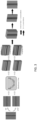
- the network structure is shown in Figure 3 .
- a deep CNN is constructed based on a modified version of the U-net with all convolutional layers and down-sampling layers changed for the receptive field restriction.
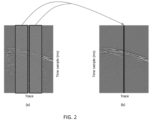
- the input seismic image is clockwise rotated twice with angles 90o and 270o so that both the left and right sections of the original receiver gather is moved upward, and they are separately inputted to the network.
- the network is composed of two parts, namely the blind-trace U-net and the merging layers, the merging layers being previously disclosed as the responsible for carrying out the combination of the two feature maps.
- the receptive field of each layer is strictly restricted to the upper half area for each row so that the model can extract the coherent features for each trace based on its left or right adjacent area in the original input respectively.
- the two output feature maps are cropped at the bottom and padded at the top such that the target traces can be excluded from its receptive field to fulfill the "blind-trace" purpose.
- a trace example is marked in black, the informative left and right areas of it at each stage are marked using two different patterns, a first pattern with inclined lines forthe left patch and a second pattern with a square grid forthe right patch respectively.
- the trace is buried under the patches, and at the end of the process, the trace will be excluded from the patches. For the edges, there is only one side of the patch that is informative and zeros are padded on the other side.
- the image is processed only once and the network gives the predictions for all traces at the same time.
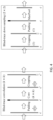
- the convolutional layers and down-sampling layers are changed as shown in figure 4 .
- the rotated inputs are projected to 32 feature maps in the first layer.
- the feature maps are doubled in the last convolutional layer of each contracting block and halved correspondingly in the expanding blocks.
- Each blind-trace convolutional layer in the encoder is replaced by a blind-trace residual block (i.e. a residual block with all convolutional layers modified).
- Batch Normalization is adopted before each activation in the decoder.
- the last two 1 ⁇ 1 convolutional layers project the concatenated 64 feature maps to 32 and 1 respectively. It has been used ReLU activation in the intermediate convolutional layers and leaky ReLU for the last 1 ⁇ 1 convolutional layer.
- the proposed blind-trace network with blending loss combines the merits of both the conventional filter-based method and the inversion-based method.
- the large number of the weights in the U-Net endows the network to achieve a complex non-linear filter to extract information from the coherent signal, meanwhile, forthe low-SNR area where filters could not obtain any coherent information, the minimization of the blending loss reconstructs the coherent signal underneath through nonlinear inversion. This is a one-stage deblending framework and does not require much exhaustive and meticulous hyperparameter tuning.
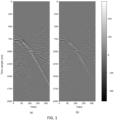
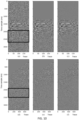
- Figures 5(d), 5(e) and 5(f) are the corresponding unblended data of that shown in figures 5(a), 5(b) and 5(c) respectively.
- the blending and pseudo-deblending is performed in the time-space by applying dithering codes to the shots, followed by summation and cropping.
- the weights and bias are randomly initialized and trained with the Adam optimizer.
- Figures 6 to 11 shows the deblending results using the blind-trace network and one-stage deblending for different blending schemes.
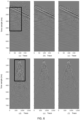
- Figure 6 presents the result of the "alternate" blending scheme. Short shifting between two consecutive shots prevents the early arrival noises from mixing with the late arrivals, but the noises distributed across the whole image.
- figure 7 a zoom-in area of figure 9 is presented. From the demonstration in both common receiver domain and common shot domain, it is shown that the one-stage deblending can effectively remove the noises for both early arrivals and late arrivals, preserving the details for both low and high-frequency patterns.
- Hyf blending scheme introduces more challenges for deblending models. Due to the concentration of the noises and long dithering time, the weak amplitudes in late arrivals are severely contaminated by strong noises from the early arrivals. As can be seen in figure 8 and the emphasized area of it in figure 9 , traditional filters tend to fail due to the loss of coherency. Besides, the heteroscedasticity problem would increase the difficulty for the iterative method, in which harsh requirements are imposed for the accuracy of amplitude estimation. As shown in figure 9(c) and (f) , the proposed method not only works as a denoising model but also acts as non-linear inversion from the blending loss with the blind-trace regularization. The signals submerged by strong blending noises are reconstructed by optimization.
- the one-stage deblending can still give a very good result as demonstrated in figure 10 and 11 .
- Blending scheme Pseudo-deblended Training-stage Tuning-stage "alternate” 0.5178 0.1594 0.1141 "half” 0.0674 0.0169 0.0072 "continuous" 0.3250 0.1176 0.0789
Landscapes
- Engineering & Computer Science (AREA)
- Physics & Mathematics (AREA)
- Life Sciences & Earth Sciences (AREA)
- General Physics & Mathematics (AREA)
- Remote Sensing (AREA)
- Theoretical Computer Science (AREA)
- Geophysics (AREA)
- General Life Sciences & Earth Sciences (AREA)
- Biomedical Technology (AREA)
- General Health & Medical Sciences (AREA)
- Health & Medical Sciences (AREA)
- Artificial Intelligence (AREA)
- Environmental & Geological Engineering (AREA)
- Biophysics (AREA)
- Computational Linguistics (AREA)
- Data Mining & Analysis (AREA)
- Evolutionary Computation (AREA)
- Geology (AREA)
- Molecular Biology (AREA)
- Computing Systems (AREA)
- General Engineering & Computer Science (AREA)
- Mathematical Physics (AREA)
- Software Systems (AREA)
- Acoustics & Sound (AREA)
- Image Processing (AREA)
- Image Analysis (AREA)
Claims (12)
- Verfahren zur Rekonstruktion mindestens einer Spur in einem seismischen Bild eines Common-Receiver- oder Common-Mid-Point-Gather oder eines Common-Offset-Gather und im Zeitbereich, wobei das Bild Spuren im Zeitbereich mit seismischen Daten, die bei einer Vermessung gewonnen wurden, und mindestens eine zu rekonstruierende Spur umfasst, wobei das Verfahren die Schritte umfasst:- Einsetzen eines neuronalen Faltungsnetzwerks zur Vorhersage einer Spur, wobei das neuronale Faltungsnetzwerk mindestens eine Schicht umfasst, wobei die mindestens eine Schicht des neuronalen Faltungsnetzwerks eine Kernfunktion mit einem rezeptiven Blindspurfeld umfasst, das benachbarte Spuren abdeckt;- Trainieren des neuronalen Faltungsnetzwerks unter Verwendung einer Vielzahl von Spuren des seismischen Bildes;- Eingeben des seismischen Bildes in das neuronale Faltungsnetzwerk, welches den Wert der mindestens einen zu rekonstruierenden Spur prognostiziert;- Zuweisen des vorhergesagten Wertes der mindestens einen zu rekonstruierenden Spur im seismischen Bild an der Stelle der zu rekonstruierenden Spur;dadurch gekennzeichnet, dassdas rezeptive Feld der Kernel-Funktion benachbarte Spuren mit Daten abdeckt, aber nicht die Spur, die sich an der Position der zu rekonstruierenden Spur befindet,das neuronale Faltungsnetz ein U-Netz ist unddas rezeptive Feld der Kernel-Funktion durch die folgenden Prozessschritte bestimmt wird:- Begrenzen des rezeptiven Feldes auf eine Seite entsprechend der Richtung der Spur;- Duplizieren des Bildes, das in das rezeptive Feld eingegeben werden soll, was zu einer ersten Kopie des Bildes und einer zweiten Kopie des Bildes führt, wobei die zweite Kopie des Bildes um 180° in Bezug auf die erste Kopie des Bildes gedreht ist;- Eingeben der ersten Kopie und der zweiten Kopie des Bildes in das rezeptive Feld des U-Netzes und Kombinieren der resultierenden Bilder zu einem einzigen Bild.
- Verfahren gemäß Anspruch 1, wobei das U-Netz mindestens eine Abwärtsabtastungsschicht umfasst, wobei die mindestens eine Abwärtsabtastungsschicht die Schicht mit einer Kernel-Funktion mit dem rezeptiven Feld der Blindspur ist.
- Verfahren gemäß einem der vorhergehenden Ansprüche, wobei die mindestens eine Schicht mit einem Blind-Trace-Rezeptionsfeld eine Down-Sampling-Schicht ist und wobei jede Schicht des neuronalen Faltungsnetzwerks ferner einen Ausgang zur Ausgabe einer Merkmalskarte umfasst, und wobei:- vor der Eingabe einer von einer vorherigen Ebene ausgegebenen Merkmalskarte oder des Bildes, wenn die aktuelle Ebene die erste Ebene ist, in die aktuelle Ebene die Merkmalskarte aufgefüllt wird, indem am Ende der Merkmalskarte an einer Seite der Kurve Reihen von Nullen hinzugefügt werden;- die Faltungsoperation durchgeführt wird;- die gleiche Anzahl von Zeilen ausgeschnitten wird, die zuvor hinzugefügt wurde, wobei das Ausschneiden der Ausgabe-Merkmalskarte auf der Seite durchgeführt wird, die der Seite gegenüberliegt, auf der zuvor Zeilen hinzugefügt wurden.
- Verfahren gemäß einem der vorhergehenden Ansprüche, wobei der Trainingsprozess des U-Netzes ein Konvergenzkriterium verwendet, das auf einer Schätzung des Approximationsfehlers Es zur Messung des Interpolationsverlustes bei der Vorhersage der rekonstruierten Spur basiert, wobei die Schätzung des Approximationsfehlers Es als eine lineare Kombination eines Misfit-Verlusts und eines Regularisierungsverlusts bestimmt wird und der Regularisierungsverlust durch die folgenden Schritte bestimmt wird:- Bestimmen des Hauptenergiebereichs des nicht rekonstruierten Bildes;- Berechnen der Norm des rekonstruierten Bildes im Frequenzbereich, der auf den Bereich beschränkt ist, der gemäß einer vorgegebenen Norm nicht Teil des Hauptenergiebereichs ist.
- Verfahren gemäß Anspruch 4, wobei die Linearkombination, die die Schätzung des Approximationsfehlers bestimmt, lautet:
Es = ∥Misfit - Verlust∥ + α∥Regularisierungsverlust∥ wobei α einen positiven Gewichtungswert und ∥·∥ die vorgegebene Norm darstellen. - Verfahren gemäß dem vorhergehenden Anspruch, wobei der Fehlanpassungsverlust nach Entfernen der rekonstruierten Spur(en) als Differenz zwischen dem nicht rekonstruierten Bild und dem rekonstruierten Bild bestimmt wird.
- Verfahren zum Deblending seismischer Daten in einem Empfängerbereich, wobei das Verfahren umfasst:a) Entfalten einer Vielzahl von Schallquellen ns an der oberen Oberfläche des Reservoirbereichs, wobei die Schallquellen ns in B Schallquellen-Gruppen σl , l = 1 ... B, zusammengefasst werden, wobei jede Schallquelle nur in einer Schallquellen-Gruppe σl und an einer Stelle

 b) Speichern jeder Schallquelle, für jede Schallquellen-Gruppe σl , l = 1 ... B, mit einer zufälligen Verzögerungszeit τli und der Antwort in den akustischen Empfängern in einer Datenstruktur, die dargestellt werden kann durch
 c) Berechnen der Fourier-Transformation
 d) Bestimmen für jede Frequenz ωk von Π LS (:,:,ωk ) = Γ*Π b (:,:, ωk ), wobei Γ*

 e) Berechnen einer inversen Fourier-Transformation von F -1(Π LS (:,:, ωk )) = Pljk ;f) Sortieren der Shot-Gather-Reihenfolge in der Ausgabe Pijk , um das Bild Ij der Trace-Daten im Common-Receiver-Bereich oder im Common-Mid-Point-Receiver-Bereich oder im Common-Offset-Receiver-Bereich und im Zeitbereich zu bekommen;g) Durchführen eines Deblending-Schritts für jede Spur durch Rekonstruktion des kohärenten Signals der Spuren unter Verwendung eines Rekonstruktionsverfahrens gemäß einem der Ansprüche 1 bis 6.
 - Verfahren zum Deblending seismischer Daten gemäß Anspruch 7, wobei
- Verfahren zum Deblending seismischer Daten gemäß Anspruch 7, wobei D = I und I die Identitätsmatrix bezeichnet.
- Verfahren zum Deblending seismischer Daten gemäß einem der Ansprüche 7 bis 9, wobei jede Quelle nur einmal aufgenommen wird und für alle m ≠ n, σm ∩ σn = ∅ gilt.
- Computerprogramm-Produkt mit Anweisungen, das bei Ausführung des Programms durch einen Computer ein Verfahren gemäß einem der Ansprüche 1 bis 10 ausführt.
- Computersystem mit mindestens einem Prozessor, der zur Ausführung eines Verfahrens gemäß einem der Ansprüche 1 bis 10 geeignet ist.
Priority Applications (3)
| Application Number | Priority Date | Filing Date | Title |
|---|---|---|---|
| ES21382674T ES3015233T3 (en) | 2021-07-23 | 2021-07-23 | Method for reconstructing at least one trace in a seismic image |
| EP21382674.6A EP4123343B1 (de) | 2021-07-23 | 2021-07-23 | Verfahren zur rekonstruktion wenigstens einer spur in einem seismischen bild |
| US17/872,776 US12287443B2 (en) | 2021-07-23 | 2022-07-25 | Method for reconstructing at least one trace in a seismic image |
Applications Claiming Priority (1)
| Application Number | Priority Date | Filing Date | Title |
|---|---|---|---|
| EP21382674.6A EP4123343B1 (de) | 2021-07-23 | 2021-07-23 | Verfahren zur rekonstruktion wenigstens einer spur in einem seismischen bild |
Publications (3)
| Publication Number | Publication Date |
|---|---|
| EP4123343A1 EP4123343A1 (de) | 2023-01-25 |
| EP4123343B1 true EP4123343B1 (de) | 2025-01-08 |
| EP4123343C0 EP4123343C0 (de) | 2025-01-08 |
Family
ID=77168156
Family Applications (1)
| Application Number | Title | Priority Date | Filing Date |
|---|---|---|---|
| EP21382674.6A Active EP4123343B1 (de) | 2021-07-23 | 2021-07-23 | Verfahren zur rekonstruktion wenigstens einer spur in einem seismischen bild |
Country Status (3)
| Country | Link |
|---|---|
| US (1) | US12287443B2 (de) |
| EP (1) | EP4123343B1 (de) |
| ES (1) | ES3015233T3 (de) |
Families Citing this family (2)
| Publication number | Priority date | Publication date | Assignee | Title |
|---|---|---|---|---|
| CN116819615B (zh) * | 2023-08-30 | 2023-11-21 | 中国石油大学(华东) | 一种地震数据重建方法 |
| CN119310625B (zh) * | 2024-12-10 | 2025-03-18 | 中国石油大学(华东) | 一种用于全波形反演的多尺度傅里叶神经算子模型 |
Citations (1)
| Publication number | Priority date | Publication date | Assignee | Title |
|---|---|---|---|---|
| US20050222774A1 (en) * | 2002-06-19 | 2005-10-06 | Jean-Claude Dulac | Method, device and software package for smoothing a subsurface property |
Family Cites Families (4)
| Publication number | Priority date | Publication date | Assignee | Title |
|---|---|---|---|---|
| US11105942B2 (en) * | 2018-03-27 | 2021-08-31 | Schlumberger Technology Corporation | Generative adversarial network seismic data processor |
| EP3894901A2 (de) * | 2018-12-11 | 2021-10-20 | Exxonmobil Upstream Research Company (EMHC-N1-4A-607) | Durch automatisierte seismische interpretation geführte invertierung |
| US11175424B2 (en) * | 2019-02-25 | 2021-11-16 | Saudi Arabian Oil Company | Seismic data de-blending |
| EP4314904A4 (de) * | 2021-03-22 | 2025-01-29 | Services Pétroliers Schlumberger | Automatische erstellung und validierung von modellen unterirdischer eigenschaften |
-
2021
- 2021-07-23 ES ES21382674T patent/ES3015233T3/es active Active
- 2021-07-23 EP EP21382674.6A patent/EP4123343B1/de active Active
-
2022
- 2022-07-25 US US17/872,776 patent/US12287443B2/en active Active
Patent Citations (1)
| Publication number | Priority date | Publication date | Assignee | Title |
|---|---|---|---|---|
| US20050222774A1 (en) * | 2002-06-19 | 2005-10-06 | Jean-Claude Dulac | Method, device and software package for smoothing a subsurface property |
Non-Patent Citations (1)
| Title |
|---|
| HUGO LEDOUX ET AL: "An Efficient Natural Neighbour Interpolation Algorithm for Geoscientific Modelling", DEVELOPMENTS IN SPATIAL DATA HANDLING: 11TH INTERNATIONAL SYMPOSIUM ON SPATIAL DATA HANDLING; SDH SYMPOSIUM, LEICESTER, 23-25 AUGUST 2004, SPRINGER, vol. 11, 1 January 2005 (2005-01-01), pages 97 - 108, XP009174041, ISBN: 978-3-540-22610-9 * |
Also Published As
| Publication number | Publication date |
|---|---|
| US12287443B2 (en) | 2025-04-29 |
| EP4123343A1 (de) | 2023-01-25 |
| ES3015233T3 (en) | 2025-04-30 |
| EP4123343C0 (de) | 2025-01-08 |
| US20230066911A1 (en) | 2023-03-02 |
Similar Documents
| Publication | Publication Date | Title |
|---|---|---|
| Sun et al. | Deep learning for low-frequency extrapolation of multicomponent data in elastic FWI | |
| US8775143B2 (en) | Simultaneous source encoding and source separation as a practical solution for full wavefield inversion | |
| EP2067112B1 (de) | Iterative umkehrung von daten aus simultanen geophysikalischen quellen | |
| US8437998B2 (en) | Hybrid method for full waveform inversion using simultaneous and sequential source method | |
| US9625593B2 (en) | Seismic data processing | |
| EP2260331B1 (de) | Effizientes verfahren zur umkehrung geophysischer daten | |
| Aghamiry et al. | ADMM-based multiparameter wavefield reconstruction inversion in VTI acoustic media with TV regularization | |
| US12287443B2 (en) | Method for reconstructing at least one trace in a seismic image | |
| Wapenaar et al. | On the relation between seismic interferometry and the simultaneous‐source method | |
| Luiken et al. | Integrating self-supervised denoising in inversion-based seismic deblending | |
| WO2010014118A1 (en) | Statistical decoding and imaging of multishot and single-shot seismic data | |
| Kaur et al. | Separating primaries and multiples using hyperbolic radon transform with deep learning | |
| Wang et al. | Closed-loop SRME based on 3D L1-norm sparse inversion | |
| SG187705A1 (en) | Hybrid method for full waveform inversion using simultaneous and sequential source method | |
| Oropeza | The singular spectrum analysis method and its application to seismic data denoising and reconstruction | |
| Liu | Multi-dimensional reconstruction of seismic data | |
| Operto et al. | Full Waveform Inversion beyond the Born approximation: A tutorial review | |
| Hu et al. | Migration deconvolution | |
| Vrolijk et al. | Source deghosting of coarsely sampled common-receiver data using machine learning | |
| Ovcharenko | Data-driven methods for the initialization of full-waveform inversion | |
| Mo et al. | Deep learning-based off-the-grid seismic data reconstruction and regularization: Preliminary research | |
| Cheng | Gradient projection methods with applications to simultaneous source seismic data processing | |
| Eaid et al. | 1D and 1.5 D internal multiple prediction in MatLab | |
| Al-Ali | Land seismic data acquisition and preprocessing | |
| Popa | Seismic Data Reconstruction With Low-rank Tensor Optimization |
Legal Events
| Date | Code | Title | Description |
|---|---|---|---|
| PUAI | Public reference made under article 153(3) epc to a published international application that has entered the european phase |
Free format text: ORIGINAL CODE: 0009012 |
|
| STAA | Information on the status of an ep patent application or granted ep patent |
Free format text: STATUS: THE APPLICATION HAS BEEN PUBLISHED |
|
| AK | Designated contracting states |
Kind code of ref document: A1 Designated state(s): AL AT BE BG CH CY CZ DE DK EE ES FI FR GB GR HR HU IE IS IT LI LT LU LV MC MK MT NL NO PL PT RO RS SE SI SK SM TR |
|
| STAA | Information on the status of an ep patent application or granted ep patent |
Free format text: STATUS: REQUEST FOR EXAMINATION WAS MADE |
|
| 17P | Request for examination filed |
Effective date: 20230421 |
|
| RBV | Designated contracting states (corrected) |
Designated state(s): AL AT BE BG CH CY CZ DE DK EE ES FI FR GB GR HR HU IE IS IT LI LT LU LV MC MK MT NL NO PL PT RO RS SE SI SK SM TR |
|
| STAA | Information on the status of an ep patent application or granted ep patent |
Free format text: STATUS: EXAMINATION IS IN PROGRESS |
|
| 17Q | First examination report despatched |
Effective date: 20230908 |
|
| REG | Reference to a national code |
Ref country code: DE Ref legal event code: R079 Free format text: PREVIOUS MAIN CLASS: G01V0099000000 Ipc: G01V0020000000 Ref country code: DE Ref legal event code: R079 Ref document number: 602021024631 Country of ref document: DE Free format text: PREVIOUS MAIN CLASS: G01V0099000000 Ipc: G01V0020000000 |
|
| GRAP | Despatch of communication of intention to grant a patent |
Free format text: ORIGINAL CODE: EPIDOSNIGR1 |
|
| STAA | Information on the status of an ep patent application or granted ep patent |
Free format text: STATUS: GRANT OF PATENT IS INTENDED |
|
| RIC1 | Information provided on ipc code assigned before grant |
Ipc: G01V 20/00 20240101AFI20240821BHEP |
|
| INTG | Intention to grant announced |
Effective date: 20240902 |
|
| GRAS | Grant fee paid |
Free format text: ORIGINAL CODE: EPIDOSNIGR3 |
|
| GRAA | (expected) grant |
Free format text: ORIGINAL CODE: 0009210 |
|
| STAA | Information on the status of an ep patent application or granted ep patent |
Free format text: STATUS: THE PATENT HAS BEEN GRANTED |
|
| AK | Designated contracting states |
Kind code of ref document: B1 Designated state(s): AL AT BE BG CH CY CZ DE DK EE ES FI FR GB GR HR HU IE IS IT LI LT LU LV MC MK MT NL NO PL PT RO RS SE SI SK SM TR |
|
| REG | Reference to a national code |
Ref country code: GB Ref legal event code: FG4D |
|
| REG | Reference to a national code |
Ref country code: CH Ref legal event code: EP |
|
| REG | Reference to a national code |
Ref country code: DE Ref legal event code: R096 Ref document number: 602021024631 Country of ref document: DE |
|
| REG | Reference to a national code |
Ref country code: IE Ref legal event code: FG4D |
|
| U01 | Request for unitary effect filed |
Effective date: 20250129 |
|
| U07 | Unitary effect registered |
Designated state(s): AT BE BG DE DK EE FI FR IT LT LU LV MT NL PT RO SE SI Effective date: 20250205 |
|
| REG | Reference to a national code |
Ref country code: ES Ref legal event code: FG2A Ref document number: 3015233 Country of ref document: ES Kind code of ref document: T3 Effective date: 20250430 |
|
| PG25 | Lapsed in a contracting state [announced via postgrant information from national office to epo] |
Ref country code: RS Free format text: LAPSE BECAUSE OF FAILURE TO SUBMIT A TRANSLATION OF THE DESCRIPTION OR TO PAY THE FEE WITHIN THE PRESCRIBED TIME-LIMIT Effective date: 20250408 |
|
| PG25 | Lapsed in a contracting state [announced via postgrant information from national office to epo] |
Ref country code: PL Free format text: LAPSE BECAUSE OF FAILURE TO SUBMIT A TRANSLATION OF THE DESCRIPTION OR TO PAY THE FEE WITHIN THE PRESCRIBED TIME-LIMIT Effective date: 20250108 |
|
| PG25 | Lapsed in a contracting state [announced via postgrant information from national office to epo] |
Ref country code: IS Free format text: LAPSE BECAUSE OF FAILURE TO SUBMIT A TRANSLATION OF THE DESCRIPTION OR TO PAY THE FEE WITHIN THE PRESCRIBED TIME-LIMIT Effective date: 20250508 |
|
| PG25 | Lapsed in a contracting state [announced via postgrant information from national office to epo] |
Ref country code: HR Free format text: LAPSE BECAUSE OF FAILURE TO SUBMIT A TRANSLATION OF THE DESCRIPTION OR TO PAY THE FEE WITHIN THE PRESCRIBED TIME-LIMIT Effective date: 20250108 |
|
| PG25 | Lapsed in a contracting state [announced via postgrant information from national office to epo] |
Ref country code: GR Free format text: LAPSE BECAUSE OF FAILURE TO SUBMIT A TRANSLATION OF THE DESCRIPTION OR TO PAY THE FEE WITHIN THE PRESCRIBED TIME-LIMIT Effective date: 20250409 |
|
| U20 | Renewal fee for the european patent with unitary effect paid |
Year of fee payment: 5 Effective date: 20250710 |
|
| PG25 | Lapsed in a contracting state [announced via postgrant information from national office to epo] |
Ref country code: SM Free format text: LAPSE BECAUSE OF FAILURE TO SUBMIT A TRANSLATION OF THE DESCRIPTION OR TO PAY THE FEE WITHIN THE PRESCRIBED TIME-LIMIT Effective date: 20250108 |
|
| PGFP | Annual fee paid to national office [announced via postgrant information from national office to epo] |
Ref country code: ES Payment date: 20250827 Year of fee payment: 5 |
|
| PGFP | Annual fee paid to national office [announced via postgrant information from national office to epo] |
Ref country code: NO Payment date: 20250729 Year of fee payment: 5 |
|
| PGFP | Annual fee paid to national office [announced via postgrant information from national office to epo] |
Ref country code: GB Payment date: 20250728 Year of fee payment: 5 |
|
| PG25 | Lapsed in a contracting state [announced via postgrant information from national office to epo] |
Ref country code: CZ Free format text: LAPSE BECAUSE OF FAILURE TO SUBMIT A TRANSLATION OF THE DESCRIPTION OR TO PAY THE FEE WITHIN THE PRESCRIBED TIME-LIMIT Effective date: 20250108 |
|
| PG25 | Lapsed in a contracting state [announced via postgrant information from national office to epo] |
Ref country code: SK Free format text: LAPSE BECAUSE OF FAILURE TO SUBMIT A TRANSLATION OF THE DESCRIPTION OR TO PAY THE FEE WITHIN THE PRESCRIBED TIME-LIMIT Effective date: 20250108 |
|
| PLBE | No opposition filed within time limit |
Free format text: ORIGINAL CODE: 0009261 |
|
| STAA | Information on the status of an ep patent application or granted ep patent |
Free format text: STATUS: NO OPPOSITION FILED WITHIN TIME LIMIT |