EP4095497A1 - Noise canceller, abnormality diagnosis device, and noise cancellation method - Google Patents
Noise canceller, abnormality diagnosis device, and noise cancellation method Download PDFInfo
- Publication number
- EP4095497A1 EP4095497A1 EP21745108.7A EP21745108A EP4095497A1 EP 4095497 A1 EP4095497 A1 EP 4095497A1 EP 21745108 A EP21745108 A EP 21745108A EP 4095497 A1 EP4095497 A1 EP 4095497A1
- Authority
- EP
- European Patent Office
- Prior art keywords
- signal
- noise
- observation
- filter
- band
- Prior art date
- Legal status (The legal status is an assumption and is not a legal conclusion. Google has not performed a legal analysis and makes no representation as to the accuracy of the status listed.)
- Pending
Links
Images













Classifications
-
- G—PHYSICS
- G01—MEASURING; TESTING
- G01H—MEASUREMENT OF MECHANICAL VIBRATIONS OR ULTRASONIC, SONIC OR INFRASONIC WAVES
- G01H1/00—Measuring characteristics of vibrations in solids by using direct conduction to the detector
- G01H1/003—Measuring characteristics of vibrations in solids by using direct conduction to the detector of rotating machines
-
- G—PHYSICS
- G01—MEASURING; TESTING
- G01M—TESTING STATIC OR DYNAMIC BALANCE OF MACHINES OR STRUCTURES; TESTING OF STRUCTURES OR APPARATUS, NOT OTHERWISE PROVIDED FOR
- G01M13/00—Testing of machine parts
- G01M13/04—Bearings
- G01M13/045—Acoustic or vibration analysis
-
- G—PHYSICS
- G01—MEASURING; TESTING
- G01M—TESTING STATIC OR DYNAMIC BALANCE OF MACHINES OR STRUCTURES; TESTING OF STRUCTURES OR APPARATUS, NOT OTHERWISE PROVIDED FOR
- G01M17/00—Testing of vehicles
- G01M17/08—Railway vehicles
-
- G—PHYSICS
- G10—MUSICAL INSTRUMENTS; ACOUSTICS
- G10K—SOUND-PRODUCING DEVICES; METHODS OR DEVICES FOR PROTECTING AGAINST, OR FOR DAMPING, NOISE OR OTHER ACOUSTIC WAVES IN GENERAL; ACOUSTICS NOT OTHERWISE PROVIDED FOR
- G10K11/00—Methods or devices for transmitting, conducting or directing sound in general; Methods or devices for protecting against, or for damping, noise or other acoustic waves in general
- G10K11/16—Methods or devices for protecting against, or for damping, noise or other acoustic waves in general
- G10K11/175—Methods or devices for protecting against, or for damping, noise or other acoustic waves in general using interference effects; Masking sound
- G10K11/178—Methods or devices for protecting against, or for damping, noise or other acoustic waves in general using interference effects; Masking sound by electro-acoustically regenerating the original acoustic waves in anti-phase
- G10K11/1785—Methods, e.g. algorithms; Devices
- G10K11/17853—Methods, e.g. algorithms; Devices of the filter
- G10K11/17854—Methods, e.g. algorithms; Devices of the filter the filter being an adaptive filter
-
- G—PHYSICS
- G01—MEASURING; TESTING
- G01H—MEASUREMENT OF MECHANICAL VIBRATIONS OR ULTRASONIC, SONIC OR INFRASONIC WAVES
- G01H17/00—Measuring mechanical vibrations or ultrasonic, sonic or infrasonic waves, not provided for in the other groups of this subclass
Definitions
- the present invention relates to a noise canceler, an abnormality diagnosis apparatus, and a noise canceling method.
- Patent Literature Document 1 discloses noise removal processing that is performed by using an adaptive filter in acoustic diagnosis using a microphone.
- An LMS (least mean square) algorithm is used as the adaptive filter.
- Patent Literature Document 2 discloses abnormality diagnosis in a rolling mill.
- an elastic wave is measured by an AE sensor in a no-load state using a press-down signal and a rotation signal, and an abnormality in a shaft and a bearing is diagnosed.
- Patent Literature Document 3 solves the problem that, in abnormality diagnosis of a railway vehicle, it is not possible to distinguish whether abnormal vibration is due to a flat spot in a wheel or due to an axle bearing, or whether it is due to the railroad track or another abnormality.
- Patent Literature Document 4 discloses an adaptive filter or an optimum filter that is used in abnormality diagnosis of a rolling apparatus.
- noise includes, for example, vibration from another machine, vibration from gears and road surfaces, vibration from an engine and a motor, vibration and sound generated from a cutting tool, a grindstone, and a workpiece in machining equipment, and noise from an ore crusher in a mining machine.
- noise and vibration may have strong unsteadiness.
- Patent Literature Documents 1 to 4 it may be difficult to obtain a signal according to which abnormality diagnosis is possible in an operation state where the above-mentioned large amount of noise is generated.
- an object of the present invention is to provide a technique by which it is possible to accurately perform abnormality diagnosis even in an operation state where a large amount of noise is generated.
- a noise canceler includes: a signal obtaining unit configured to obtain an observation signal obtained by sampling vibration of an apparatus; a signal delay unit configured to obtain a delay signal by delaying the observation signal obtained by the signal obtaining unit; and a Kalman filter processing unit configured to apply, to the observation signal and the delay signal, a Kalman filter that adapts a filter coefficient so as to reduce a residual signal between the observation signal and an estimated signal estimated based on the observation signal and the delay signal using an adaptive filter, and to output the residual signal.
- this noise canceler a weak signal that is necessary for abnormality diagnosis and is buried in a large amount of noise is extracted to a desired signal as an error (residual) between an observation signal and an estimated signal.
- the noise canceler preferably includes a band-limiting unit configured to band-limit the observation signal and the delay signal from a lower limit frequency that removes a direct current signal component, to an upper limit frequency set to half or less of a sampling frequency.
- the Kalman filter serving as the adaptive filter works effectively by band-limiting the observation signal and the delay signal.
- the noise canceler preferably further includes a down-conversion unit configured to convert the frequency of a signal band-limited by the band-limiting unit to a low frequency.
- a down-conversion unit configured to convert the frequency of a signal band-limited by the band-limiting unit to a low frequency.
- the down-conversion unit realizes down-conversion by performing complex multiplication between an input signal and a periodic signal having a frequency that corresponds to a conversion amount. Down-conversion is easily realized through complex multiplication.
- the down-conversion unit performs complex multiplication using pre-stored numerical value data that corresponds to the periodic signal. By using the pre-stored numerical value data, the amount of calculation can be further reduced.
- the noise canceler preferably includes an FFT processing unit configured to implement envelope FFT processing on the residual signal output from the Kalman filter processing unit.
- an FFT processing unit configured to implement envelope FFT processing on the residual signal output from the Kalman filter processing unit.
- the Kalman filter processing unit uses the filter coefficient as a state vector and uses an identity matrix as a state transition matrix.
- identity matrix is used as the transition matrix, the calculation structure in the filter is simplified.
- the Kalman filter processing unit uses a variance matrix of system noise and a variance of observed noise in the Kalman filter as time-varying parameters and estimates the variance matrix and the variance in parallel with the adaptation of the filter coefficient. Due to the variance matrix and the variance being estimated as time-varying parameters, the variance matrix and the variance naturally converge or transition to appropriate parameter values, and therefore the trouble of adjusting the parameter values is eliminated.
- An abnormality diagnosis apparatus includes: the above-described noise canceler; and a diagnosis unit for diagnosing whether or not there is an abnormality in the apparatus using the residual signal obtained by the noise canceler.
- this abnormality diagnosis apparatus According to this abnormality diagnosis apparatus, a weak signal necessary for abnormality diagnosis is taken out from noise by the noise canceler, and therefore highly-accurate diagnosis becomes possible.
- a noise canceling method includes: a signal obtaining step of obtaining an observation signal obtained by sampling vibration of an apparatus; a signal delay step of obtaining a delay signal by delaying the observation signal obtained by the signal obtaining step; and a Kalman filter processing step of applying, to the observation signal and the delay signal, a Kalman filter that adapts a filter coefficient so as to reduce a residual signal between the observation signal and an estimated signal estimated based on the observation signal and the delay signal using an adaptive filter, and outputting the residual signal.
- the noise canceler is a noise canceler using one sensor (using the input of one sensor)
- the abnormality diagnosis apparatus is an abnormality diagnosis apparatus including a noise canceler using one sensor
- the noise canceling method is a noise canceling method using one sensor.
- ALE adaptive line enhancer
- the periodic signal component is estimated using the adaptive line enhancer (ALE)
- the vibration of the rolling bearing is extracted as an error (residual).
- the noise canceler is used to measure vibration from railroad seams, vibration from road seams, irregular vibration from an ore crushing machine, or the like, it is preferable to use a Kalman filter or an NLMS as an adaptive filter and combine a Fourier analyzer. If the vibration to be measured is unsteady vibration, it includes a waveform that decays in a short time even if a very large amplitude is generated, but for example, by adjusting the basic parameters of the normalized LMS, a noise canceler that uses the input of one sensor can be configured as described above.
- the Kalman filter converges quickly and can quickly and accurately follow time-varying signals and noise.
- noise canceler abnormality diagnosis apparatus, and noise canceling method
- a weak signal that is necessary for abnormality diagnosis and is buried in a large amount of noise is extracted to a desired signal as an error (residual) between the observation signal and the estimated signal.
- the noise canceler includes: a signal obtaining unit configured to obtain measurement signals obtained by sampling vibration at a plurality of locations that are side by side in a direction along a rotation axis of a rotation apparatus, at a distance from each other in the direction; a band-limiting unit configured to band-limit the measurement signals obtained by the signal obtaining unit, from a lower limit frequency that removes a direct current signal component, to an upper limit frequency set to half or less of a sampling frequency; and an adaptive filter processing unit configured obtain an estimated signal by applying an adaptive filter to an observation signal that is one of the measured signals band-limited by the band-limiting unit and a reference signal that is another one of the measured signals, adapt a filter coefficient of the adaptive filter so as to reduce a residual signal between the observation signal and the estimated signal, and output the residual signal.
- the noise canceler may further include an FFT processing unit configured to implement envelope FFT processing on the residual signal output from the adaptive filter processing unit.
- the adaptive filter processing unit may use a Kalman filter as the adaptive filter.
- the Kalman filter may use the filter coefficient as a state vector and use an identity matrix as a state transition matrix.
- the adaptive filter processing unit may use a variance matrix of system noise and a variance of observed noise in the Kalman filter as time-varying parameters and estimate the variance matrix and the variance in parallel with the adaptation of the filter coefficient.
- the adaptive filter processing unit may use a normalized LMS as the adaptive filter.
- An abnormality determination apparatus includes: the noise canceler according to the fourth aspect described above; and a diagnosis unit configured to diagnose whether or not there is an abnormality in the rotation apparatus using the residual signal obtained by the noise canceler.
- a noise canceling method includes: a signal obtaining step of obtaining measurement signals obtained by sampling vibration at a plurality of locations that are side by side in a direction along a rotation axis of a rotation apparatus, at a distance from each other in the direction; a band-limiting step of band-limiting the measurement signals obtained in the signal obtaining step, from a lower limit frequency that removes a direct current signal component, to an upper limit frequency set to half or less of a sampling frequency; and an adaptive filter processing step of obtaining an estimation signal by applying an adaptive filter to an observation signal that is one of the measured signals band-limited in the band-limiting step and a reference signal that is another one of the measured signals, adapt a filter coefficient of the adaptive filter so as to reduce a residual signal between the observation signal and the estimation signal, and output the residual signal.
- abnormality diagnosis can be performed more accurately even in an operation state where a large amount of noise is generated.
- Figs. 1A, 1B , and 1C are diagrams illustrating a first embodiment of an abnormality diagnostic apparatus of the present invention.
- Fig. 1A schematically shows a plan view of a truck (railway bogie) 200 for a railroad vehicle, which is the target of abnormality diagnosis in this embodiment, and a rail 201.
- Fig. 1B schematically shows a side view of a wheel 202 of the truck 200 and the rail 201.
- Fig. 1C shows a configuration of an abnormality diagnosis apparatus 100.
- the abnormality diagnosis apparatus 100 of this embodiment is a device for performing abnormality diagnosis on a bearing unit 204 in the truck 200.
- the truck 200 has, for example, four wheels 202, carries the main body of the railroad vehicle, and travels on the rail 201. Each wheel 202 rolls on the rail 201 without slipping and rotates around an axle 203. Each axle 203 connects two wheels 202, and the wheels 202 are fixed to the axle 203.
- the truck 200 has a bearing unit 204, which includes double-row tapered roller bearings (not shown) at locations corresponding to each wheel 202. The double-row tapered roller bearings rotatably hold the axles 203.
- Each bearing unit 204 is equipped with a vibration acceleration sensor 105 that detects vibration acceleration in a direction perpendicular to the outer circumferential surface of the bearing.
- the vibration acceleration sensor 105 is arranged at a position suitable for detecting the vibration generated in the bearing accompanying a defect such as a scratch when such a defect occurs in the bearing, and for example, shock vibration that occurs when the wheel 202 passes a seam 205 of the rail 201 enters the vibration acceleration sensor 105 as a large amount of noise.
- the abnormality diagnosis apparatus 100 includes a vibration acceleration sensor 105 as shown in Fig. 1C . It should be noted that the abnormality diagnosis apparatus according to this embodiment may be a device that does not have the vibration acceleration sensor 105 and obtains an observation signal obtained by such a sensor, for example, as recorded data.
- the abnormality diagnosis apparatus 100 further includes a noise canceler 101, a sensor amplifier 102, a digital oscilloscope 103, and a personal computer 104.
- the sensor amplifier 102 amplifies a signal of the vibration detected by the vibration acceleration sensor 105 and outputs the result to the noise canceler 101.
- the noise canceler 101 obtains a vibration signal (observation signal from the vibration acceleration sensor 105) from the sensor amplifier 102, and cancels the noise through filter processing, which will be described in detail later.
- the noise canceler 101 corresponds to an embodiment of the noise canceler of the present invention.
- the digital oscilloscope 103 has an envelope FFT processing function, and performs envelope FFT processing on a signal in which noise has been canceled by the noise canceler 101.
- the envelope FFT processing carried out by the digital oscilloscope 103 corresponds to the function of the FFT processing unit according to the embodiment of the present invention, and the combination of the noise canceler 101 and the digital oscilloscope 103 also corresponds to one embodiment of the noise canceler of the present invention.
- the personal computer 104 performs abnormality diagnosis of the bearing unit 204 using the signal subjected to envelope FFT processing.
- the personal computer 104 has a display.
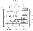
- Fig. 2 is a diagram showing a structure of the noise canceler 101.
- the noise canceler 101 includes an input circuit 111, a DIP switch 112, a one-chip microcomputer 113, an RC filter 114, a BNC connector 115 for input, and BNC connectors 116A and 116B for output.
- the input circuit 111 includes an input buffer, a low-pass RC filter, and the like, obtains an observation signal via the BNC connector 115 for input, and outputs the observation signal to the one-chip microcomputer 113.
- the signal obtaining unit in this embodiment of the present invention corresponds to, for example, the BNC connector 115, the input circuit 111, and an AD converter (ADC) 121 with a built-in one-chip microcomputer.
- ADC AD converter
- the DIP switch 112 includes, for example, a 3-bit switch for selecting a band of a band-pass filter that narrows the band of a signal input to the adaptive filter.
- the DIP switch 112 also includes a 1-bit switch that switches between a case where a plurality of observation signals obtained from a plurality of vibration acceleration sensors 105 are used and a case where one observation signal obtained from one vibration acceleration sensor 105 is used.
- the observation signal will be described as being a signal obtained from one vibration acceleration sensor 105.
- the RC filter 114 mitigates a case in which the output signal becomes a stepped shape and prevents electrical disturbance noise from being mixed in.
- the output signal from the noise canceler 101 is output via the RC filter 114 and the BNC connectors 116A and 116B for output.
- the one-chip microcomputer 113 implements filter processing through so-called digital signal processing on the observation signal input from the input circuit 111, and generates an output signal in which noise has been canceled.
- the one-chip microcomputer 113 includes an AD converter 121, a DA converter (DAC) 122, a ROM 123, a RAM 124, and a processor 125, which is a CPU or DSP.
- the one-chip microcomputer 113 also has a JTAG 126 and a UART 127 as input/output interfaces.
- the UART 127 is used, for example, for reading out a signal record before FFT processing and the like, and the JTAG 126 is used, for example, for rewriting a program and the like, but detailed description thereof will be omitted.
- the AD converter 121 converts an analog observation signal into a digital signal
- the DA converter 122 converts the processed digital signal into an analog signal.
- the ROM 123 stores programs to be executed by the processor 125 and constants, and the RAM 124 stores the values of variables to be used by the processor 125 in program execution.
- the processor 125 performs filtering processing through digital processing.
- As the filter processing processing of a high-pass filter, a low-pass filter, and an adaptive filter is performed.
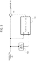
- An adaptive filter 130 is a filter that estimates a noise signal yk, which is a noise component in an observation signal dk, based on the observation signal dk and a delay signal xk of the observation signal dk.
- the observation signal dk is, for example, a signal in which the noise signal yk is mixed with a desired signal sk (not shown) representing vibration accompanying a defect in the bearing unit 204.
- the signal obtained from the vibration acceleration sensor 105 is used as the observation signal dk, and the signal obtained by delaying the observation signal using a delay device 140 is used as the delay signal xk.
- the role of the delay device 140 is played by a storage device (RAM 124) incorporated in the one-chip microcomputer 113, and the delay device 140 is subjected to software processing.
- This storage device (memory) is an example of the signal delay unit of the present invention, and due to a signal being stored, the past signal remains in the present, whereby a delay is obtained.
- the data length of the delay signal to be stored is determined by the number of delays and the order of the filter. A data matrix including the data length is updated using the observation signal obtained every hour.
- the update of this data matrix is performed by manipulating the data in the memory using the processor 125, but the details thereof are omitted here.
- the correlation between the sinusoidal noise components included in the observation signal dk and the delay signal xk is high, and the irregular vibration signal component of the bearing unit 204 does not correlate with the observation signal dk and the delay signal xk.
- the estimated signal indicates a sinusoidal noise signal yk estimated by the adaptive filter.
- a Kalman filter is adopted as the adaptive filter 130, and in the Kalman filter, the noise signal yk is estimated by estimating a filter coefficient of the adaptive filter 130 described below.
- Fig. 4 is a diagram showing a configuration concept of the adaptive filter 130.
- the adaptive filter 130 in this embodiment includes a Kalman filter processing unit 131 and time-varying elements.
- the time-varying elements include an update unit 132 that updates an observation matrix cTk, a first estimation unit 133 that estimates a variance matrix Qk of system noise, and a second estimation unit 134 that estimates a variance Rk of observed noise.
- the observation matrix cTk is a definite matrix based on a delay signal dk-delay serving as the delay signal xk obtained with the elapse of time, and is expressed by the following equation (1).
- xk dk-delay.
- c T k x k ⁇ 1 , ... , x k ⁇ N
- the data length of the observation matrix is N, but in actuality, it is also necessary to store the delay of the observation signal.
- the noise signal yk is expressed by the following equation (2).
- the order (number of taps) N of the filter is, for example, 6.
- Equation (2) shows that the noise signal yk is estimated by a linear combination of the delay signals xk-1, xk-2, ..., xk-N, which are past signals.
- a sine wave can be estimated using equation (2).
- Equation (3) is an equation of state, and the filter coefficient hk can be changed over time in a system model according to equation (3), and unsteady signals and noise can be estimated through estimation with the Kalman filter.
- dk indicates the observed value.
- vk is observed noise, which is Gaussian white noise with an average of zero.
- the state space model is set by equations (3) and (4).
- hk is a filter coefficient, which is a state vector to be sequentially estimated by the Kalman filter.
- a variance matrix Qk is expressed by the system noise wk of equation (3).
- the variance Rk is expressed by the observed noise vk in equation (4).
- Q k E w k ⁇ w k T
- R k E ⁇ k 2
- the variance matrix Qk of the system noise and the variance Rk of the observed noise serve as adjustment parameters in the Kalman filter that estimates the filter coefficient hk.
- the filter coefficient hk is estimated as a state estimation value h (with ⁇ )k through the prediction step and the filtering step.
- a preliminary state estimated value h (with ⁇ ) -k and a preliminary error covariance matrix P-k are calculated by the following equations (7) and (8) with the transition matrix as an identity matrix.
- the Kalman gain gk, the state estimation value h (with ⁇ ) k, and a subsequent error covariance matrix Pk are calculated by the following equations (9), (10), and (11).
- the residual signal ek dk-cTkh (with ⁇ ) k is calculated and output as the estimated value of the desired signal sk (bearing vibration).
- dk-cTkh (with ⁇ ) -k in the parentheses of the second term on the right side of equation (10) indicates the preliminary output estimation error, and this preliminary output estimation error may be used as a desired signal to replace the residual signal ek.
- the time-varying parameters Qk and Rk are used as the variance matrix of the system noise and the variance of the observed noise, and sequential estimation thereof is performed by the first estimation unit 133 and the second estimation unit 134.
- the variance matrix Qk of the system noise wk and the variance Rk of the observed noise vk that are used in the Kalman filter may also be used as adjustment parameters. It is more preferable that the variance matrix Qk and the variance Rk are used in a certain range for noise cancelation.
- Time-varying parameters Qk and Rk may be used instead of the time-varying parameters Qk and Rk as the variance matrix of the system noise and the variance of the observed noise, but when the time-varying parameters Qk and Rk are used, the variance matrix of the system noise and the variance of the observed noise naturally change or converge to appropriate values together with the estimation of the filter coefficient hk. Accordingly, it is desirable that the time-varying parameters Qk and Rk are used as the variance matrix of the system noise and the variance of the observed noise. Alternatively, after the time-varying parameters Qk and Rk have changed or converged to appropriate values, the parameter values may be fixed for the purpose of reducing the amount of calculation and the like.
- the variance matrix Q (with ⁇ ) k of the system noise is estimated by the following equation (12)
- the variance R (with ⁇ ) k of the observed noise is estimated by the following equation (13).
- the coefficient ⁇ is a fixed value within the range of 0 ⁇ ⁇ 1
- the residual signal ek is a value calculated by the following equation (14)
- each of the variance matrix Q (with ⁇ ) k and the variance R (with ⁇ ) k is estimated.
- Fig. 5 is a flowchart showing the noise canceling procedure.
- the procedure of Fig. 5 starts from the initialization of the one-chip microcomputer 113 and the like performed by turning on the power, for example.
- step S101 the observation signal dk, which is a measurement signal, is converted via the input circuit 111 and the AD converter 121, and the converted observation signal dk is acquired in the RAM 124 as block data through DMA.
- the sampling frequency of the AD converter 121 is, for example, 36 kHz.
- step S102 a 12-bit integer with a sampling frequency of 36 kHz is converted to a 32-bit floating point number.
- step S103 the processor 125 performs high-speed calculation of processing of a 50th-order FIR low-pass filter (gain 1 at 2.5 kHz or less) in order to remove a frequency band of 4.5 kHz or more (i.e., in order to obtain a gain of -50 dB or less).
- the sampling frequency is decimated by one-fourth, from 36 kHz to 9 kHz.
- step S104 the processor 125 further applies 17th-order high-pass filter processing to the observation signal dk down-sampled to 9 kHz.
- the observation signal dk is band-limited by the low-pass filter processing in step S103 and the high-pass filter processing in step S104, the number of sine waves, which are periodic noise to be estimated by the adaptive line enhancer that is the noise canceler, is narrowed down in the observation signal dk.
- the specific band in the low-pass filter processing and the high-pass filter processing needs to be adjusted to some extent according to the type of the target apparatus for which the abnormality diagnosis is performed, the driving condition, and the like. Since this adjustment can be handled by manual adjustment using the DIP switch 112, detailed description thereof will be omitted here.
- the processing in which step S103 and step S104 are combined corresponds to an example of the processing performed by the band-limiting unit according to the present invention.
- the band-limiting unit according to the present invention may limit the band through so-called band-pass filter processing.
- step S105 Based on the observation signal dk that has been band-limited in this manner, in step S105, a delay signal xk for the observation signal dk is generated.
- step S106 the observation signal dk that has been subjected to the processing of step S104 and the delay signal xk are the inputs of the adaptive filter 130.
- step S106 Kalman filter processing, which is the internal structure of the adaptive filter 130, is executed. Then, the residual signal ek is output as a signal from which noise has been removed.
- step S107 the residual signal ek is sent as block data to the DA converter 122 through DMA, and is converted into an analog residual signal ek at a sampling frequency of 9 kHz.
- steps S101 to S107 is repeatedly executed while the observation signal dk is obtained as a measurement signal. While steps S101 to S107 are repeatedly executed, the residual signal ek converted by the DA converter 122 is subjected to envelope FFT processing by the digital oscilloscope 103 in step S108, and becomes a spectral signal used for diagnosis. Then, the spectral signal that is the processing result is output from the digital oscilloscope 103 to the personal computer 104 and is used for abnormality diagnosis.
- first and second order frequencies indicating the abnormality within a range of an allowable error
- the diagnosis result obtained by the personal computer 104 may be displayed on a display, for example, and may be confirmed by a user of the abnormality diagnosis apparatus 100, or may be transmitted or notified to an administrator (a person who is not the user of the abnormality diagnosis apparatus 100) from the personal computer 104 via a network or the like.
- the diagnosis result obtained by the personal computer 104 may be recorded in a recording location (device) that can be later confirmed by the user or the like of the abnormality diagnosis apparatus 100, for example.
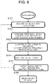
- This comparative example is a procedure in which noise cancelation by an adaptive filter is omitted in the abnormality diagnosis apparatus 100 of this embodiment.
- Fig. 6 is a flowchart showing the procedure of the comparative example.
- the envelope FFT is performed after decimation by an FIR low-pass filter and high-pass filter processing. That is, in the procedure shown in Fig. 6 , step S101, step S102, step S103, and step S104 are executed in the same manner as in the procedure shown in Fig. 5 . However, after that, there is no noise removal performed through delay processing corresponding to step S105 in Fig. 5 and Kalman filter processing corresponding to step S106, and the processing proceeds from step S104 to step S107 and step S108.
- Figs. 7A and 7B are illustrative views showing a time signal in the abnormality diagnosis apparatus of this embodiment.
- Fig. 7A shows a graph of the observation signal obtained from the vibration acceleration sensor 105 shown in Fig. 2
- Fig. 7B shows a graph of the residual signal obtained by the abnormality diagnosis apparatus 100 of this embodiment.
- the horizontal axis of each graph represents time, and the vertical axis represents signal amplitude.
- the impact is transmitted to the bearing unit 204 each time the rolling element (not shown) of the bearing passes the defect (e.g., a flaw) in the track surface of the bearing and a pulsed waveform 152 is generated every cycle in which the rolling element (e.g., a roller) passes the defect location.
- This observation signal is a signal obtained by subjecting the signal obtained from the vibration acceleration sensor 105 to the processing of the comparative example shown in Fig. 6 . Specifically, FIR filtering processing of a high-pass filter and a low-pass filter is applied.
- the waveform 151 of the vibration generated at the seam 205 of the rail 201 has a large amplitude but is a narrow band waveform
- the waveform can be estimated by an adaptive filter of a small order.
- the waveforms 152 of the vibrations generated by the defect of the bearing unit 204 are wide band waveforms and cannot be estimated by an adaptive filter of a small order. For this reason, in noise estimation using an adaptive filter of a limited order, only the waveform 151 of the rail seam 205 is estimated, and therefore the waveforms 152 of the bearing defect remain in the residual signal obtained by subtracting the estimated signal from the observation signal (i.e., the calculation result obtained by equation (14)).
- the residual signal shown in Fig. 7B is obtained as the residual signal.
- the waveform 151 of the rail seam 205 is mostly removed, and mainly the waveforms 152 of the bearing defect are extracted.
- Fig. 8A shows a graph of the spectral signal of the observation signal obtained by the abnormality diagnosis apparatus 100
- Fig. 8B shows a graph of the spectral signal of the residual signal obtained by the abnormality diagnosis apparatus 100.
- the horizontal axis of each graph represents frequency, and the vertical axis represents signal strength.
- the spectral signals shown in the graph of Fig. 8A and the graph of Fig. 8B are obtained by implementing envelope FFT processing on each of the observation signal and the residual signal shown in the graph of Fig. 7A and the graph of Fig. 7B .
- the graphs of Figs. 8A and 8B show a schematic image in which the spectral signal is smoothed in the frequency domain.
- the noise canceling processing in this embodiment is realized by automatic estimation of the time-varying parameters Qk and Rk, but the system noise Q and the observed noise R may be fixed values obtained through trial and error. However, there are fewer mistakes in automatic adjustment performed using equations (12) and (13). Conventionally, in the Kalman filter, the variances of system noise and observed noise needed to be input as adjustment parameters. On the other hand, in the noise canceler of the embodiment of the present invention, highly-accurate noise canceling processing is realized by a data-driven algorithm in which a method of automatically estimating system noise and observed noise works favorably.
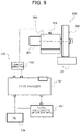
- Fig. 9 is a diagram showing another application example of the abnormality diagnosis apparatus 100.
- Fig. 9 shows the abnormality diagnosis apparatus 100, which is also shown in Fig. 1C , and further shows a grinding machine 300 as a diagnosis target in place of the truck 200.
- the grinding machine 300 includes a motor 301, a rotary grindstone 302, and a bearing portion 303 having a built-in spindle bearing.
- a workpiece W is ground by pressing the workpiece W against the outer circumferential surface of the rotary grindstone 302.
- mechanical noise natural vibration and whirling of a shaft of the motor 301, whirling of the rotary grindstone 302, natural vibration of an overhang shaft, and the like occur. Also, the mechanical noise in the grinding machine 300 changes depending on whether the rotary grindstone 302 is in contact with the workpiece W or not.
- the vibration acceleration sensor 105 of the abnormality diagnosis apparatus 100 is fixed to the outer surface of the bearing portion 303.
- the observation signal dk is obtained by this vibration acceleration sensor 105.
- the abnormality diagnosis apparatus 100 can perform the above-described processing based on the obtained observation signal dk to cancel the large amount of mechanical noise generated in the grinding machine 300. As a result, it is possible to accurately diagnose an abnormality such as a scratch on the spindle bearing of the bearing portion 303, for example.
- the bearing unit 204 includes a double-row tapered roller bearing, but the bearing unit 204 may include a bearing other than a double-row tapered roller bearing.
- the abnormality diagnosis apparatus of the second embodiment is, for example, an abnormality diagnosis apparatus incorporated in an industrial machine vehicle such as a dump truck, the industrial machine vehicle serving as the diagnosis target.
- Fig. 10 is a diagram showing a dump truck 400 in which the abnormality diagnosis apparatus 500 ( Fig. 11 ) of the second embodiment is incorporated.
- the dump truck 400 is an industrial machine vehicle in which, for example, ore is loaded in a vessel 401 and which is driven by rear wheels 402.
- the drive of the rear wheel 402 is executed by the rotation of the drive shaft of the rear wheel being transmitted to the wheel and the tire via a speed reducer installed on the inner circumference of the wheel.
- a speed reducer installed on the inner circumference of the wheel.
- an outer ring rotates integrally with the wheel, and an inner ring is fixed together with a drive shaft and a differential case.
- Fig. 11 is a diagram showing an abnormality diagnosis apparatus 500 incorporated in the dump truck 400 shown in Fig. 10 .
- the abnormality diagnosis apparatus 500 shown in Fig. 11 is, for example, a device for diagnosing a wheel bearing.
- the vibration acceleration sensor 505 of the abnormality diagnosis apparatus 500 is attached to a case 403 of a drive shaft to which the inner ring of the wheel bearing is fixed, with the direction perpendicular to the rotation axis of the bearing as the vibration detection direction.
- the abnormality diagnosis apparatus 500 is mounted in a vehicle as a part of the function of an ECU (engine control unit).
- the abnormality diagnosis apparatus 500 includes a microcomputer 501 and an input circuit 502 including a sensor amplifier and an analog filter.
- the microcomputer 501 includes an AD converter 511, a timer counter 512, a ROM 513, an SRAM 514, a backup SRAM 515, a CAN interface 516, a UART 517, and a processor 518.
- the AD converter 511 receives the observation signal of the vibration acceleration sensor 505 via the input circuit 502, and samples the received observation signal.
- the timer counter 512 counts a vehicle speed pulse 404 output from an encoder of the dump truck 400 to obtain the rotational speed of the bearing to be diagnosed. According to the rotation speed obtained in this manner, the characteristic frequency at a time of abnormality of the bearing is recognized.
- the CAN interface 516 can communicate with various parts of the dump truck 400 via a CAN bus 405 of an in-vehicle network. Note that if the vehicle speed is obtained from the in-vehicle network, the timer counter 512 is unnecessary and the CAN interface 516 is used.
- a multifunction display 406 is connected to the CAN bus 405, and the CAN interface 516 displays the diagnosis result of the abnormality diagnosis apparatus 500 on the multifunction display 406 via the CAN bus 405.
- the ROM 513 stores a program that performs signal processing as a noise canceler, envelope FFT processing, and abnormality diagnosis processing.
- the processor 518 performs digital processing according to this program.
- the processor 518 includes a CPU or a DSP.
- Temporary data used for each of the above-described processes is stored in the SRAM 514.
- As the SRAM 514 an SRAM having a sufficiently large capacity is used.
- the backup SRAM 515 is an SRAM to which a battery is attached, and diagnosis results and diagnosis conditions are stored in the backup SRAM 515.
- the UART 517 is used for reading records created by a personal computer or the like and changing the setting of the diagnostic conditions.
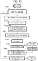
- Fig. 12 is a flowchart showing a procedure of abnormality diagnosis in the abnormality diagnosis apparatus 500.
- the same reference numerals are used for the same steps as in the first embodiment ( Fig. 5 ).
- step S301 after S106 the residual signal is subjected to processing of an FIR low-pass filter, and decimation. As a result, the number of processing points in the envelope FFT processing is suppressed, and the processing calculation becomes lighter.
- step S302 the envelope FFT processing is executed, and in step S303, the pulsed waveforms 152 as shown in Fig. 7A are detected and a frequency corresponding to the pulse cycle is obtained.
- step S401 which is performed in parallel with each of the above processes, the timer counter 512 counts the encoder pulse and the rotation speed of the shaft and the bearing is calculated.
- step S304 the peak frequency obtained in step S302 is compared with the characteristic frequency of the inner ring scratch recognized based on the rotation speed calculated in step S401, and the degree of coincidence is calculated and stored in the backup SRAM 515.
- the degree of coincidence calculated in this manner corresponds to the diagnosis result, and the degree of coincidence being high indicates that an abnormality such as an inner ring scratch has occurred.
- step S305 the diagnosis result is transmitted to and displayed on the multifunction display 406 via the CAN interface 516 and the CAN bus 405.
- the processing of each step described above is repeatedly executed while the engine of the dump truck 400 is running.
- the driver or the like of the dump truck 400 can find out whether or not there is an abnormality in a bearing or the like by checking the display of the multifunction display 406.
- the abnormality diagnosis apparatuses 100 and 500 shown in Figs. 1C and 10 are realized by inexpensive apparatuses such as embedded computers mounted in a railway vehicle and a dump truck, and diagnose abnormalities in bearings or the like through real-time processing.
- the Kalman filter is superior in ease of use and accuracy compared to an LMS, it requires a large amount of calculation, and therefore ingenuity to reduce the amount of calculation is desired in order to realize the abnormality diagnosis apparatuses 100 and 500 with inexpensive apparatuses such as embedded computers.
- a processing procedure for reducing the amount of calculation is executed before the signal processing performed using the Kalman filter.
- the configuration of the abnormality determination apparatus of the third embodiment may employ the configuration of the abnormality determination apparatus 100 of the first embodiment, or the configuration of the abnormality determination apparatus 500 of the second embodiment.
- the same reference numerals are used for the same processing and the like as in the first embodiment and the second embodiment. It is assumed that the sampling frequency of the AD converter 121 is 24 kHz.
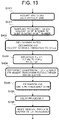
- Fig. 13 is a flowchart including a processing procedure for reducing the amount of calculation.
- the flowchart of Fig. 13 shows steps corresponding to steps S101 to S 106 in the flowcharts of Figs. 5 and 12 , and the steps other than S101 to S106 use steps and procedures shown in Fig. 5 or 12 .
- step S101 is executed and the observation signal dk is acquired as in the first embodiment and the second embodiment.
- step S401 the processing corresponding to step S102 is performed, but unlike step S102, a 12-bit integer having a sampling frequency of 24 kHz is converted to a 32-bit floating point number.
- step S402 the processing corresponding to step S103 is performed. Specifically, FIR low-pass filter processing is performed, and thereafter decimation is performed.
- the frequency component of 6 kHz or more is substantially cut off to -40 dB or less, and thus the influence of aliasing is avoided.
- the passband where attenuation does not occur in the FIR low-pass filter is, for example, from DC to 4 kHz, the sampling frequency can be lowered to 12 kHz by decimation. This is a decimation of one half for the sampling frequency of 24 kHz in step S401.
- step S403 FIR band-pass filter processing is executed.
- the passband of the band-pass is 1.7 kHz to 3.0 kHz, and the bandwidth is less than 1.5 kHz.
- Figs. 14A and 14B are graphs schematically showing the operation of the band-pass filter (FIR band-pass filter processing).
- the horizontal axes of the graphs of Figs. 14A and 14B show the frequency, and the vertical axes show the signal strength.
- Fig. 14A shows a graph 610 of the observation signal dk
- Fig. 14B shows a graph of a band portion 640 that has passed through the band-pass filter 630.
- the graph 610 of the observation signal dk extends from the DC component to half of the sampling frequency fs, and the band 620 including the signal component necessary for abnormality diagnosis such as bearings is a part of it.
- the passband of the band-pass filter 630 is set to the band 620 of the signal component required for abnormality diagnosis.
- step S404 the band-pass filter processing is executed in step S403 of Fig. 13 , and thereafter frequency down-conversion is performed in step S404.
- the frequency down-conversion is specifically realized through complex multiplication described in detail below.
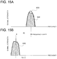
- Figs. 15A and 15B are graphs schematically showing the action of frequency down-conversion.
- the horizontal axes of the graphs of Figs. 15A and 15B show the frequency, and the vertical axes show the signal strength.
- Fig. 15A shows a graph of the band portion 640 before the down-conversion
- Fig. 15B shows a graph of the band portion 650 after the down-conversion. Since the bandwidth of the band-pass filter described as an example in step S403 of Fig. 13 is less than 1.5 kHz, there is a band without a frequency component on the DC side relative to the band portion 640 before down-conversion.
- the band portion 640 is shifted to the low frequency side by a frequency f0 so as to eliminate such a band without a frequency component.
- the band portion 650 after down-conversion falls into a frequency domain that is half or less of a new sampling frequency fs', which is significantly lower than the initial sampling frequency fs. If the bandwidth is less than 1.5 kHz, the new sampling frequency fs' may be reduced to 3 kHz.
- step S404 of Fig. 13 down-conversion is realized through complex multiplication.
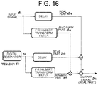
- Fig. 16 is a diagram showing a processing concept of down-conversion through complex multiplication.
- the observation signal dk corresponding to the band portion 640 that has been subjected to the band-pass filter processing shown in Fig. 15A is subjected to complexification processing.
- an imaginary part dik is calculated based on the observation signal dk by an FIR Hilbert transform filter.
- This filter coefficient can be calculated by commercially-available or free software, and detailed description here is omitted.
- a sine wave zk having a frequency f0 corresponding to the shift amount of the frequency shift (conversion) is oscillated by using a digital resonator as an oscillator.
- the details of sine wave oscillation performed by a digital resonator are omitted, but since a sine wave can be generated by a gradual equation and the amplitude and frequency can be specified by the initial value, it is convenient to generate a sine wave of any frequency.
- the sine wave zk is also complexified through FIR Hilbert transform filter processing and delay processing to obtain the real part zrk and the imaginary part zik.
- the observation signal dk and the sine wave zk complexified in this manner are subjected to complex multiplication. That is, as shown in the following equation (15), the real part drk and the real part zrk are multiplied, the imaginary part dik and the imaginary part zik are multiplied, and the multiplication results are added to each other to obtain the observation signal Dk (real part) subjected to down-conversion.
- D k d rk ⁇ z rk + d ik ⁇ z ik
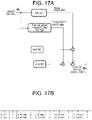
- Fig. 17A is a diagram showing a processing concept of down-conversion using a numerical table.
- step S404 of Fig. 13 The down-conversion described above is performed in step S404 of Fig. 13 .
- the observation signal Dk obtained by down-conversion has a frequency band upper limit of 1.5 kHz or less and a lower limit of DC or more. Accordingly, even if the sampling frequency (corresponding to the sampling frequency fs' shown in Fig. 15B ) is lowered to 3 kHz, the signal content is not influenced. For this reason, in step S405 of Fig. 13 , the sampling frequency of 12 kHz is decimated to one-fourth, and the sampling frequency becomes 3 kHz.
- the observation signal that has undergone down-conversion and decimation is used as the new observation signal dk, and the processing of steps S105 and S106 is executed as in the first and second embodiments, but since the sampling frequency is reduced, the amount of calculation in steps S105 and S106 is greatly reduced. Accordingly, real-time operation is possible even with an inexpensive embedded computer.
- step S107 If the third embodiment is applied to the first embodiment, the processing proceeds to step S107 after step S106. If the third embodiment is applied to the second embodiment, the processing proceeds to step S301 after step S106.
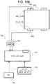
- Figs. 18A and 18B are diagrams illustrating an abnormality diagnosis apparatus 700 according to the fourth embodiment of the present invention.
- Fig. 18A schematically shows a plan view of a railway bogie to be the target of abnormality diagnosis in this embodiment and a rail
- Fig. 18B shows a configuration of the abnormality diagnosis apparatus 700.
- the fourth embodiment is a variation of the first embodiment, and the same configurations and processing are designated by the same reference numerals.
- the side view of the railway bogie and the rail in Fig. 18A is the same as in Fig. 1B .
- the abnormality diagnosis apparatus 700 of this embodiment is an apparatus for performing an abnormality diagnosis on the bearing unit 204 in the truck 200.
- description of items that are the same as in the first embodiment will be omitted as appropriate, and the description will be focused on the differences from the first embodiment.
- a vibration acceleration sensor 105 that detects vibration acceleration in a direction perpendicular to the outer peripheral surface of the bearing is attached to each bearing unit 204.
- the function of the vibration acceleration sensor 105 is the same as that of the first embodiment.
- the abnormality diagnosis apparatus 700 includes two vibration acceleration sensors 105 (105_1 and 105_2) as shown in Fig. 18B .
- One of the two vibration acceleration sensors 105 is a noise-canceled observation sensor 105_1 and the other is a reference sensor 105_2. That is, the observation signal obtained by the observation sensor 105_1 and the reference signal obtained by the reference sensor 105_2 are input to the abnormality diagnosis apparatus 700.
- the abnormality diagnosis apparatus 700 may include three or more vibration acceleration sensors 105.
- the two vibration acceleration sensors 105 included in the abnormality diagnosis apparatus 700 are provided in the bearing unit 204 corresponding to each of the two wheels 202 connected by the same axle 203. Accordingly, if the wheel 202 goes over the seam 205 of the rail 201, the two vibration accelerometers 105 will receive vibrations that correlate with each other.
- the two vibration acceleration sensors 105 included in the abnormality diagnosis apparatus 700 are provided side by side in the lengthwise direction of the axle 203 (axis direction) at two locations separated in that direction. Due to being arranged side by side in the same direction, the two vibration acceleration sensors 105 have the same phase in the rotation of the axle 203, and the two vibration acceleration sensors 105 pick up acceleration vibration in the same direction, and therefore the signal correlation becomes stronger.
- the abnormality diagnosis apparatus 700 includes the noise canceler 101, the sensor amplifier 102, the digital oscilloscope 103, and the personal computer 104.
- the sensor amplifier 102 amplifies the signal of the vibration detected by the observation sensor 105_1 and the reference sensor 105_2, and outputs the amplified signal to the noise canceler 101.
- the noise canceler 101 obtains the observation signal (after amplification) from the observation sensor 105_1 and the reference signal (after amplification) from the reference sensor 105_2, and cancels the noise through filter processing, which will be described in detail later.
- This noise canceler 101 corresponds to an embodiment of the noise canceler of the present invention.
- the functions of the digital oscilloscope 103 and the personal computer 104 are the same as those in the first embodiment.
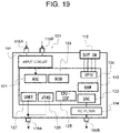
- Fig. 19 is a diagram showing the structure of the noise canceler 101.
- the noise canceler 101 includes the input circuit 111, the DIP switch 112, the one-chip microcomputer 113, the RC filter 114, BNC connectors 115A and 115B for input, and BNC connectors 116A and 116B for output.
- the input circuit 111 includes an input buffer, a low-pass RC filter, and the like, and obtains an observation signal and a reference signal via the input BNC connectors 115A and 115B and outputs them to the one-chip microcomputer 113.
- the signal acquisition unit refers to the BNC connectors 115A and 115B, the input circuit 111, and the AD converter 121 with a built-in one-chip microcomputer.
- the DIP switch 112 includes, for example, a 3-bit switch for selecting a band of a band-pass filter that narrows the band of a signal input to the adaptive filter. Also, the DIP switch 112 includes a 1-bit switch that switches between whether to use signals obtained from different vibration acceleration sensors 105, or to use a delay signal and a non-delay signal obtained from the same vibration acceleration sensor 105 as the observation signal and the reference signal. However, in this embodiment, the observation signal and the reference signal are described as being signals obtained from vibration acceleration sensors 105 that are different from each other.
- the RC filter 114 mitigates a case in which the output signal becomes a stepped signal, and prevents electrical disturbance noise from being mixed in.
- the output signal from the noise canceler 101 is output via the RC filter 114 and the BNC connectors 116A and 116B for output.
- the one-chip microcomputer 113 implements filter processing on the observation signal and the reference signal input from the input circuit 111 through so-called digital signal processing, and outputs an output signal in which noise is canceled.
- the one-chip microcomputer 113 includes an AD converter 121, a DA converter 122, a ROM 123, a RAM 124, a processor 125, a JTAG 126, and a UART 127.
- the AD converter 121 converts an analog observation signal and an analog reference signal into digital signals
- the DA converter 122 converts the processed digital signals into analog signals.
- the functions of the ROM 123 and the RAM 124 are the same as those of the first embodiment.
- the processor 125 performs filter processing through digital processing.
- As the filter processing processing of a high-pass filter, a low-pass filter, and an adaptive filter is performed.
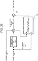
- Fig. 20 is a diagram showing the processing concept of the adaptive filter.
- the adaptive filter 150 is a filter that estimates the noise component vk in the observation signal dk based on the observation signal dk in which the noise signal from the noise source via an unknown transmission path ⁇ hi ⁇ is mixed in the desired signal sk, and the reference signal xk close to the noise source.
- the reference signal xk is ideally a noise-only signal that does not include the desired signal sk, but it is difficult to obtain such an ideal reference signal. For this reason, in practice, a reference signal xk that contains the same kind of noise with respect to the observation signal dk and has a different ratio of the desired signal sk is used.
- the observation signal dk and the reference signal xk as described above are obtained by the two vibration acceleration sensors 105 provided on the two bearing units 204 located at both ends of one axle 203.
- the estimated signal is the noise signal yk estimated by the adaptive filter 150.
- a Kalman filter is adopted as the adaptive filter 150, and in the Kalman filter, the noise signal yk is estimated by estimating the unknown transmission path ⁇ hi ⁇ . Estimating the unknown transmission path is equivalent to estimating the filter coefficients of the adaptive filter described below.
- Fig. 21 is a diagram showing the configuration concept of the adaptive filter 150 using the Kalman filter.
- the adaptive filter 150 in this embodiment includes a Kalman filter main body (Kalman filter processing unit) 131 and a time-varying element.
- the time-varying elements include an update unit 132 that updates the observation matrix cTk constituted by vectors that are past time series of the reference signal, a first estimation unit 133 that estimates the variance matrix Qk of the system noise, and a second estimation unit 134 that estimates the variance Rk of the observation noise.
- the observation matrix cTk is a definite matrix obtained based on the reference signal xk obtained over time, and is expressed by the following equation (17).
- c T k x k ⁇ 1 , ... , x k ⁇ N
- the order (number of taps) N of the filter is, for example, 10.
- a state space model which is a basic model of the Kalman filter.
- the change over time in the filter coefficient hk is expressed by the equation of state shown in the following equation (19).
- an identity matrix is used as the transition matrix, which simplifies the calculation structure in the Kalman filter processing unit 131.
- the filter coefficient hk can be changed over time in the model of equation (19), and the estimation by the Kalman filter enables the estimation of an unsteady signal and noise.
- wk vector
- cTk c T k h k + ⁇ k
- dk indicates the observed value.
- vk represents observed noise, which is Gaussian white noise with an average of zero.
- the state space model is set by equations (19) and (20).
- the state variable vector in this state space model is the filter coefficient hk, which is estimated sequentially by the Kalman filter.
- Equation (21) The variance matrix Qk of the system noise wk in equation (19) is expressed by equation (21) below.
- the variance Rk of the observed noise vk in equation (20) is expressed by equation (22) below.
- Q k E w k ⁇ w k T
- R k E ⁇ k 2
- the variance matrix Qk of the system noise and the variance Rk of the observed noise function as adjustment parameters in the Kalman filter that estimates the filter coefficient hk.
- the filter coefficient hk is estimated as the state estimation value h (with ⁇ ) k through a prediction step and a filtering step.
- the prediction step the pre-state estimated value h (with ⁇ ) -k and the pre-error covariance matrix P-k are calculated by the following equations (23) and (24) with the transition matrix as the identity matrix.
- h ⁇ k ⁇ h ⁇ k ⁇ 1
- P k ⁇ P k ⁇ 1 + Q k
- the Kalman gain gk, the state estimation value h (with ⁇ ) k, and the post-error covariance matrix Pk are calculated by the following equations (25), (26), and (27).
- the residual signal ek dk-cTkh (with ⁇ ) k is calculated and output as the estimated value of the desired signal (bearing vibration) as shown in the following equation (30).
- This residual signal is a residual signal obtained by using the subsequent estimation value obtained at a time k in equation (26) as a filter coefficient. Note that dk-cTkh (with ⁇ ) -k in equation (26) indicates a prior output estimation error, and this prior output estimation error may be used as a desired signal in place of the residual signal ek.
- the variance matrix of the system noise and the variance of the observed noise which are parameters of the Kalman filter
- the variance matrix of the system noise and the variance of the observed noise are considered to be adjustment parameters, and although it is not necessary to set highly accurate values, it is desirable that they fall within the range of a certain order to achieve the purpose of noise cancelation.
- the time-varying parameters Qk and Rk are respectively used as the variance matrix of the system noise and the variance of the observed noise, and sequential estimation is performed by the first estimation unit 133 and the second estimation unit 134.
- the fixed values Q and R of the system noise may be used instead of the time-varying parameters Qk and Rk as the variance matrix of the system noise and the variance of the observed noise
- the time-varying parameters Qk and Rk are used, the variance matrix of the system noise and the variance of the observed noise naturally converge or change to appropriate values together with the estimation of the filter coefficient hk. Accordingly, it is desirable that the time-varying parameters Qk and Rk are used as the variance matrix of the system noise and the variance of the observed noise.
- the parameter values may be fixed for the purpose of reducing the amount of calculation or the like.
- a variance matrix estimation value Q (with ⁇ ) k of the system noise is estimated by the following equation (28)
- a variance estimation value R (with ⁇ ) k of the observed noise is estimated by equation (29).
- the coefficient ⁇ is a fixed value within the range of 0 ⁇ ⁇ 1
- the residual signal ek is a value calculated by the following equation (30)
- the variance matrix Q (with ⁇ ) k and the variance R (with ⁇ ) k are estimated.
- Fig. 22 is a flowchart showing a noise canceling procedure.
- the procedure of Fig. 22 starts from the initialization of the one-chip microcomputer 113 or the like by turning on the power, for example.
- step S501 the observation signal dk and the reference signal xk obtained by converting the measurement signal obtained from the vibration acceleration sensor 105 via the input circuit 111 and the AD converter 121 are acquired as block data in the RAM 124 through DMA.
- the sampling frequency of the AD converter 121 is, for example, 36 kHz.
- step S502 a 12-bit integer with a sampling frequency of 36 kHz is converted to a 32-bit floating point number.
- step S503 the processor 125 performs high-speed calculation of processing of a 50th-order FIR low-pass filter (gain 1 of 2.5 kHz or less) in order to remove the frequency band of 4.5 kHz or more (i.e., in order to obtain a gain of -50 dB or less).
- the sampling frequency is decimated by one-fourth, from 36 kHz to 9 kHz.
- step S504 the processor 125 further performs 60th-order high-pass filter processing on the observation signal dk and the reference signal xk down-sampled to 9 kHz.
- the observation signal dk and the reference signal xk are band-limited through the low-pass filter processing in step S503 and the high-pass filter processing in step S504, the number of sine waves to be combined is narrowed down in the observation signal dk and the reference signal xk, irregularity is mitigated and the signal and noise are easy to estimate.
- the specific band in the low-pass filter processing and the high-pass filter processing needs to be adjusted to some extent according to the type of the target apparatus for which abnormality diagnosis is performed, the driving condition, and the like.
- a high-pass filter for DC removal and a low-pass filter for decimation are required.
- DC removal is processing that is essential before envelope processing. Since the amount of calculation of the adaptive filter can be reduced in proportion to the decimation rate by performing appropriate decimation processing, hurdles for realizing Kalman filter processing in real time with a microcomputer are lowered. Since it is necessary to complicate the analog filter when using a low sampling frequency from the AD conversion stage, it is advantageous to perform decimation with an FIR low-pass filter from a high sampling frequency. In this case, the filter processing at the decimated low sampling frequency is sufficient.
- step S503 and step S504 corresponds to the band-limiting unit referred to in the present invention.
- the band-limiting unit according to the present invention may limit the band through so-called band-pass filter processing.
- step S505 the Kalman filter processing, which is the internal structure of the adaptive filter 150, is executed by the processor 125. Then, the residual signal ek is output as a signal from which noise has been removed.
- step S506 the residual signal ek is sent as block data to the DA converter 122 through DMA, and is converted into an analog residual signal ek at a sampling frequency of 9 kHz.
- steps S501 to S506 is repeatedly executed while the observation signal dk and the reference signal xt are obtained. While the steps S501 to S506 are repeatedly executed, the residual signal ek converted by the DA converter 122 is subjected to the envelope FFT processing by the digital oscilloscope 103 in step S507 to become a spectral signal used for diagnosis. Then, the spectral signal that is the processing result is output from the digital oscilloscope 103 to the personal computer 104 and is used for abnormality diagnosis.
- the diagnosis result obtained by the personal computer 104 may be displayed on a display, for example, to be confirmed by the user of the abnormality diagnosis apparatus 700, or may be transmitted/notified to an administrator or the like via a network or the like. Alternatively, the diagnosis result may be recorded in a recording apparatus that can be later confirmed by a user of the abnormality diagnosis apparatus 700, for example. Also, as shown in Fig. 18B , when used for bearing diagnosis in the truck 200, it is desirable that the diagnostic system including the abnormality diagnosis apparatus 700 is mounted in the railroad vehicle.
- This comparative example is a procedure in which noise cancelation performed by an adaptive filter is omitted in the abnormality diagnosis apparatus 700 of this embodiment.
- Fig. 23 is a flowchart showing the procedure of the comparative example.
- the envelope FFT is performed after decimation by an FIR low-pass filter and high-pass filter processing. That is, in the procedure shown in Fig. 23 , steps S501 to S504 are executed in the same manner as in the procedure shown in Fig. 22 . However, thereafter, there is no noise removal through Kalman filter processing corresponding to step S505 in Fig. 22 , and the processing proceeds from step S504 to step S506 and step S507.
- Figs. 24A, 24B , and 24C are diagrams showing time signals in the abnormality diagnosis apparatus 700 of this embodiment.
- Fig. 24A shows a schematic graph of the reference signal obtained from the reference sensor 105_2 shown in Fig. 18B
- Fig. 24B shows a schematic graph of the observation signal obtained from the observation sensor 105_1 shown in Fig. 18B
- Fig. 24C shows a schematic graph of the residual signal obtained by the abnormality diagnosis apparatus 700 of this embodiment.
- the horizontal axis of each graph represents time, and the vertical axis represents signal amplitude.
- the graph of the reference signal ( Fig. 24A ) mainly shows the waveform 251 of the vibration generated in the axle 203 when the wheel 202 passes the seam 205 of the rail 201 shown in Fig. 1B .
- the graph of the observation signal ( Fig. 24B ) shows the waveform 251 of vibration caused by the seam 205 of the rail 201, and the pulsed waveform 252 caused by a defect such as a scratch on the bearing.
- a defect occurs in the track surface of the bearing, an impact is transmitted to the vibration acceleration sensor 105 to which the bearing unit 204 is attached each time the rolling element (e.g., roller) of the bearing passes the defect (e.g., a scratch or peeling) on the track surface of the bearing, and a pulsed waveform 252 is generated every cycle of the rolling element (e.g., a roller) passing the defect location.
- the rolling element e.g., roller
- the reference signal and the observation signal shown in the graphs of Figs. 24A and 24B are signals obtained by subjecting the signal obtained from the vibration acceleration sensor 105 to the processing of the comparative example shown in Fig. 23 . Specifically, FIR filtering processing of a high-pass filter and a low-pass filter is applied.
- the waveform 251 of the vibration caused by the rail seam 205 cannot be attenuated even if the difference between the observation signal and the reference signal is taken, in this embodiment, the waveform 251 is attenuated by an adaptive filter.
- the residual signal shown in the graph of Fig. 24C is obtained as the residual signal.
- the waveform 251 of the rail seam 205 is mostly removed, and the waveform 252 of the bearing defect is mainly extracted.
- Fig. 25A is a diagram showing a graph of the spectral signal of the observation signal obtained by the abnormality diagnosis apparatus 700
- Fig. 25B is a diagram showing a graph of the spectral signal of the residual signal obtained by the abnormality diagnosis apparatus 700.
- each graph represents frequency
- the vertical axis represents signal strength
- the spectral signals shown in the graphs of Figs. 25A and 25B are obtained by implementing envelope FFT processing on each of the observation signal shown in the graph of Fig. 24B and the residual signal shown in the graph of Fig. 24C .
- the graphs of Figs. 25A and 25B represent a schematic image in which the spectral signal is smoothed in the frequency domain.
- the graph of the observation signal of Fig. 25A shows noise 253 that gradually increases toward zero frequency, and this noise 253 is noise corresponding to the vibration generated at the rail seam 205.
- the noise 253 of the rail seam 205 is significantly reduced, and the frequency peaks 254 and 255 of the vibration generated by the defect of the bearing (not shown) become clear.
- the frequency peak 254 on the low frequency side is the peak of the fundamental wave corresponding to the frequency at which the rolling element pass the defect on the outer ring track surface of the axle bearing
- the frequency peak 255 on the high frequency side is the peak of the second harmonic.
- an algorithm for a UD decomposition filter that is numerically stabilized by an equivalent algorithm may be used instead of the standard algorithm described in detail before, and even in that case, the variance (matrix) estimation of the system noise and the observed noise shown in equations (28) and (29) can be performed in the same manner.
- the noise canceling processing in this embodiment is realized by automatic estimation of the time-varying parameters Qk and Rk, but the system noise Q and the observed noise R may be fixed values obtained through trial and error. However, there are fewer mistakes in the automatic adjustment performed using equations (28) and (29).
- the Kalman filter is used as an adaptive filter, the noise removal ability is more excellent compared to that of the NLMS algorithm described below.
- the Kalman filter is superior to the NLMS in terms of both convergence speed and tracking. Also, with a Kalman filter, it is not necessary for the user (creator) to determine the step size parameter for updating the filter coefficient, and the optimum step size is substantially automatically determined by the calculation of the Kalman gain, and therefore the Kalman filter is easy to use.
- the noise canceler of this embodiment highly accurate noise canceling processing is realized by a data-driven algorithm in which a method of automatically estimating the system noise and the observation noise works favorably.
- the positions of the observation sensor 105_1 and the reference sensor 105_2 described with reference to Fig. 18B are not limited to the positions shown in Fig. 18B .
- the reference sensor 105_2 side shown in Fig. 18B is used as an observation sensor to obtain an observation signal
- the observation sensor 105_1 side is used as a reference sensor to obtain a reference signal, whereby it is possible to perform abnormality diagnosis.
- the vibration signals of both bearings do not have a correlation. For this reason, one bearing that is a target of noise removal can be diagnosed regardless of whether or not there is a defect in another bearing.
- the reference sensor 105_2 may be provided at a different position from the four bearings, but the observation sensor 105_1 and the reference sensor 105_2 are preferably provided on each bearing corresponding to each of the two wheels 202 connected by one axle 203. This is because, as described above, in the truck 200, two wheels 202 are fixed to one axle 203 and rotate together, and therefore, in addition to the vibration received by the wheels from the rail 201, the vibration from the vehicle such as the drive gear also tends to be correlated vibration in the bearings at both ends of one axle 203. When such correlated vibration enters the observation sensor 105_1 and the reference sensor 105_2 as noise, the vibration signal caused by the bearing defect is effectively extracted as an error signal through the noise removal.
- a normalized LMS is used instead of the Kalman filter.
- the fifth embodiment is a variation of the fourth embodiment.
- the same reference numerals will be used for the same configurations and processes as in the fourth embodiment.
- the step size in the LMS (least mean squares) algorithm varies according to the magnitude of the input signal (i.e., the variance of the noise). Since the processing content in the normalized LMS is known, description thereof is omitted here, but by using the normalized LMS for the adaptive filter 150, as described above, sequential estimation of the transmission path [hi] is performed such that the difference between the noise component yk and the observation signal dk is as small as possible.
- the estimation of the transmission path ⁇ hi ⁇ obtained by the normalized LMS is executed as an estimation of the filter coefficient hk as in the case of the Kalman filter, but the normalized LMS uses multiple fixed parameters for the sequential estimation. The specific value of this fixed parameter is adjusted to an appropriate value according to the type of the target device for which the abnormality diagnosis is performed, the driving condition, and the like.
- Fig. 26 is a flowchart showing a noise canceling procedure in this embodiment in which the normalized LMS is used.
- step S501, step S502, step S503, and step S504 are executed in the same manner as in the procedure shown in Fig. 22 . Thereafter, instead of the Kalman filter processing in step S505 of Fig. 22 , the normalized LMS (NLMS) processing is executed in step S601. Then, the processing proceeds to step S506 and step S507.
- NLMS normalized LMS
- Fig. 27A is a diagram showing a graph of the spectral signal of the observation signal obtained in the comparative example
- Fig. 27B is a diagram showing the spectral signal of the residual signal.
- the graph in Fig. 27A is the same as the graph in Fig. 25A .
- the graph of Fig. 27B shows a graph of the smoothing spectrum of the residual signal obtained by performing noise cancelation using the NLMS algorithm based on the observation signal and the reference signal in the procedure shown in Fig. 26 .
- the LMS algorithm including the NLMS algorithm can adapt to an unstable signal and noise, and therefore although it is inferior to a Kalman filter, it can remove the noise 253 of the rail seam 205 from the observation signal similarly to the Kalman filter, and the vibrations 254 and 255 caused by the defect in the bearing become clear.
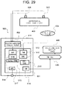
- Fig. 28 is a diagram showing an example in which the abnormality diagnosis apparatus 700 is applied to a grinding machine 300.
- the grinding machine 300 includes a motor 301, a rotary grindstone 302, and a bearing portion 303 having a built-in spindle bearing.
- the configuration of the grinding machine 300 is the same as that of the grinding machine 300 described with reference to Fig. 9 .
- the observation sensor 105_1 and the reference sensor 105_2 of the abnormality diagnosis apparatus 700 are fixed at two locations arranged side by side in the direction along the rotation axis of the motor 301 and the rotary grindstone 302 at a distance from each other in that direction.
- the observation signal dk and reference signal xk are obtained by the observation sensor 105_1 and the reference sensor 105_2.
- the abnormality diagnosis apparatus 700 can perform the above-described processing based on the observation signal dk and the reference signal xt obtained in this manner, and can cancel the large amount of mechanical noise generated in the grinding machine 300. As a result, it is possible to accurately diagnose an abnormality such as a scratch on the spindle bearing of the bearing portion 303, for example.
- the sixth embodiment described below is an abnormality diagnosis apparatus incorporated in the dump truck 400 of Fig. 10 .
- This embodiment is a variation of the fourth embodiment and is a variation of the second embodiment.
- the same reference numerals are used for the same structures and processes as those in the second embodiment.
- Fig. 29 is a diagram showing an abnormality diagnosis apparatus 800 incorporated in the dump truck 400 shown in Fig. 10 .
- the abnormality diagnosis apparatus 800 shown in Fig. 29 is, for example, an apparatus for performing diagnosis on a wheel bearing.
- the abnormality diagnosis apparatus 800 includes two acceleration vibration sensors 505 and 506, and the two acceleration vibration sensors 505 and 506 are attached to the case 403 of the drive shaft to which the inner wheel of the wheel bearing is fixed, with the direction perpendicular to the rotation shaft of the bearing as the vibration detection direction.
- the two acceleration vibration sensors 505 and 506 one is the right rear wheel sensor 505 and the other is the left rear wheel sensor 506. Since the wheel bearing whose rotation axis extends in the left-right direction of the vehicle body is the target of diagnosis, the two acceleration vibration sensors 505 and 506 are arranged side by side in the left-right direction of the vehicle body at a distance from each other in the left-right direction.
- the abnormality diagnosis apparatus 800 is mounted in the vehicle as a part of the function of the ECU (engine control unit).
- the abnormality diagnosis apparatus 800 includes a microcomputer 501 and an input circuit 502 including a sensor amplifier and an analog filter.
- the microcomputer 501 includes an AD converter 511, a timer counter 512, a ROM 513, an SRAM 514, a backup SRAM 515, a CAN interface 516, a UART 517, and a processor 518.
- the AD converter 511 receives the measurement signals of the two acceleration vibration sensors 505 and 506 via the input circuit 502 and samples the received measurement signals. Of the two measurement signals, one is used as the observation signal dk and the other is used as the reference signal xk.
- the timer counter 512, the CAN interface 516, the ROM 513, the processor 518, the SRAM 514, the backup SRAM 515, and the UART517 are the same as those described with reference to Fig. 11 .
- Fig. 30 is a flowchart showing the procedure of abnormality diagnosis in the abnormality diagnosis apparatus 800.
- step S505 the residual signal is subjected to FIR low-pass filter processing and decimation in step S701. As a result, the number of processing points in the envelope FFT processing is reduced, and the processing calculation is lighter.
- step S702 the envelope FFT processing is executed, and in step S703, the peak as indicated by the arrow in graph 252 of Fig. 24B is detected and the peak frequency is obtained.
- step S801 which is performed in parallel with each of the above processes, the timer counter 512 counts the encoder pulse and the rotation speed of the shaft and the bearing is calculated.
- step S704 the peak frequency obtained in step S702 and the characteristic frequency of the inner ring scratch recognized based on the rotation speed calculated in step S801 are compared with each other, and the degree of coincidence is calculated and stored in the backup SRAM 515.
- the degree of coincidence calculated in this manner corresponds to the diagnosis result, and the degree of coincidence being high indicates that an abnormality such as an inner ring scratch has occurred.
- step S705 the diagnosis result is transmitted to and displayed on the multifunction display 406 via the CAN interface 516 and the CAN bus 405.
- the processing of each step described above is repeatedly executed while the engine of the dump truck 400 is running.
- the driver or the like of the dump truck 400 can find out whether or not there is an abnormality in a bearing or the like by checking the display of the multifunction display 406.
- the fifth embodiment may also be applied to the sixth embodiment. That is, the Kalman filter of the sixth embodiment may be replaced with a normalized LMS. Also, the fifth embodiment may be applied to the first to third embodiments.
Landscapes
- Physics & Mathematics (AREA)
- General Physics & Mathematics (AREA)
- Acoustics & Sound (AREA)
- Engineering & Computer Science (AREA)
- Multimedia (AREA)
- Measurement Of Mechanical Vibrations Or Ultrasonic Waves (AREA)
- Testing Of Devices, Machine Parts, Or Other Structures Thereof (AREA)
- Steering Control In Accordance With Driving Conditions (AREA)
- Power Steering Mechanism (AREA)
Abstract
Description
- The present invention relates to a noise canceler, an abnormality diagnosis apparatus, and a noise canceling method.
- Conventionally, a diagnosis apparatus for diagnosing an abnormality or the like in a bearing in a rotation apparatus has been proposed.
- For example,
Patent Literature Document 1 discloses noise removal processing that is performed by using an adaptive filter in acoustic diagnosis using a microphone. An LMS (least mean square) algorithm is used as the adaptive filter. - For example,
Patent Literature Document 2 discloses abnormality diagnosis in a rolling mill. In this abnormality diagnosis, an elastic wave is measured by an AE sensor in a no-load state using a press-down signal and a rotation signal, and an abnormality in a shaft and a bearing is diagnosed. - For example,
Patent Literature Document 3 solves the problem that, in abnormality diagnosis of a railway vehicle, it is not possible to distinguish whether abnormal vibration is due to a flat spot in a wheel or due to an axle bearing, or whether it is due to the railroad track or another abnormality. - For example, Patent Literature Document 4 discloses an adaptive filter or an optimum filter that is used in abnormality diagnosis of a rolling apparatus.
-
- Patent Literature Document 1:
Japanese Patent Application Laid-Open No. H11-271181 - Patent Literature Document 2:
Japanese Patent Application Laid-Open No. 2010-234403 - Patent Literature Document 3:
Japanese Patent Application Laid-Open No. 2007-278894 - Patent Literature Document 4:
Japanese Patent Application Laid-Open No. 2008-164578 - From the viewpoint of production efficiency, it is desirable to perform diagnosis during the operation of the rotation apparatus, but in a machine that requires abnormality diagnosis for a bearing or the like, a large amount of noise may be constantly generated depending on the operation environment. Such noise includes, for example, vibration from another machine, vibration from gears and road surfaces, vibration from an engine and a motor, vibration and sound generated from a cutting tool, a grindstone, and a workpiece in machining equipment, and noise from an ore crusher in a mining machine. Such noise and vibration may have strong unsteadiness.
- With the techniques of
Patent Literature Documents 1 to 4, it may be difficult to obtain a signal according to which abnormality diagnosis is possible in an operation state where the above-mentioned large amount of noise is generated. - In view of this, an object of the present invention is to provide a technique by which it is possible to accurately perform abnormality diagnosis even in an operation state where a large amount of noise is generated.
- In order to solve the above-described problems, a noise canceler according to a first aspect of the present invention includes: a signal obtaining unit configured to obtain an observation signal obtained by sampling vibration of an apparatus; a signal delay unit configured to obtain a delay signal by delaying the observation signal obtained by the signal obtaining unit; and a Kalman filter processing unit configured to apply, to the observation signal and the delay signal, a Kalman filter that adapts a filter coefficient so as to reduce a residual signal between the observation signal and an estimated signal estimated based on the observation signal and the delay signal using an adaptive filter, and to output the residual signal.
- According to this noise canceler, a weak signal that is necessary for abnormality diagnosis and is buried in a large amount of noise is extracted to a desired signal as an error (residual) between an observation signal and an estimated signal.
- The noise canceler preferably includes a band-limiting unit configured to band-limit the observation signal and the delay signal from a lower limit frequency that removes a direct current signal component, to an upper limit frequency set to half or less of a sampling frequency. The Kalman filter serving as the adaptive filter works effectively by band-limiting the observation signal and the delay signal.
- The noise canceler preferably further includes a down-conversion unit configured to convert the frequency of a signal band-limited by the band-limiting unit to a low frequency. By converting the frequency of the signal to a low band, the amount of calculation in the Kalman filter processing unit is reduced, and real-time operation is possible even with an inexpensive device such as an embedded computer.
- In the noise canceler, it is preferable that the down-conversion unit realizes down-conversion by performing complex multiplication between an input signal and a periodic signal having a frequency that corresponds to a conversion amount. Down-conversion is easily realized through complex multiplication.
- In the noise canceler, it is preferable that the down-conversion unit performs complex multiplication using pre-stored numerical value data that corresponds to the periodic signal. By using the pre-stored numerical value data, the amount of calculation can be further reduced.
- The noise canceler preferably includes an FFT processing unit configured to implement envelope FFT processing on the residual signal output from the Kalman filter processing unit. By implementing the envelope FFT processing on the residual signal, it is easy to confirm a signal having a characteristic frequency accompanying an abnormality in the apparatus.
- It is preferable that the Kalman filter processing unit uses the filter coefficient as a state vector and uses an identity matrix as a state transition matrix. When the identity matrix is used as the transition matrix, the calculation structure in the filter is simplified.
- It is preferable that the Kalman filter processing unit uses a variance matrix of system noise and a variance of observed noise in the Kalman filter as time-varying parameters and estimates the variance matrix and the variance in parallel with the adaptation of the filter coefficient. Due to the variance matrix and the variance being estimated as time-varying parameters, the variance matrix and the variance naturally converge or transition to appropriate parameter values, and therefore the trouble of adjusting the parameter values is eliminated.
- An abnormality diagnosis apparatus according to a second aspect of the present invention includes: the above-described noise canceler; and a diagnosis unit for diagnosing whether or not there is an abnormality in the apparatus using the residual signal obtained by the noise canceler.
- According to this abnormality diagnosis apparatus, a weak signal necessary for abnormality diagnosis is taken out from noise by the noise canceler, and therefore highly-accurate diagnosis becomes possible.
- A noise canceling method according to a third aspect of the present invention includes: a signal obtaining step of obtaining an observation signal obtained by sampling vibration of an apparatus; a signal delay step of obtaining a delay signal by delaying the observation signal obtained by the signal obtaining step; and a Kalman filter processing step of applying, to the observation signal and the delay signal, a Kalman filter that adapts a filter coefficient so as to reduce a residual signal between the observation signal and an estimated signal estimated based on the observation signal and the delay signal using an adaptive filter, and outputting the residual signal.
- For example, the noise canceler is a noise canceler using one sensor (using the input of one sensor), the abnormality diagnosis apparatus is an abnormality diagnosis apparatus including a noise canceler using one sensor, and the noise canceling method is a noise canceling method using one sensor. This is an application of an adaptive line enhancer (ALE). Since the delay signal plays a role of eliminating the correlation between the observation signal and an irregular signal component, the irregular component serving as an error (residual) with respect to the periodic signal component obtained from the adaptive line enhancer (ALE) can be regarded as the vibration of a rolling bearing.
- In this manner, if the periodic signal component is estimated using the adaptive line enhancer (ALE), the vibration of the rolling bearing is extracted as an error (residual).
- Also, if the noise canceler is used to measure vibration from railroad seams, vibration from road seams, irregular vibration from an ore crushing machine, or the like, it is preferable to use a Kalman filter or an NLMS as an adaptive filter and combine a Fourier analyzer. If the vibration to be measured is unsteady vibration, it includes a waveform that decays in a short time even if a very large amplitude is generated, but for example, by adjusting the basic parameters of the normalized LMS, a noise canceler that uses the input of one sensor can be configured as described above. The Kalman filter converges quickly and can quickly and accurately follow time-varying signals and noise.
- According to this noise canceler, abnormality diagnosis apparatus, and noise canceling method, a weak signal that is necessary for abnormality diagnosis and is buried in a large amount of noise is extracted to a desired signal as an error (residual) between the observation signal and the estimated signal.
- The noise canceler according to the fourth aspect of the present invention includes: a signal obtaining unit configured to obtain measurement signals obtained by sampling vibration at a plurality of locations that are side by side in a direction along a rotation axis of a rotation apparatus, at a distance from each other in the direction; a band-limiting unit configured to band-limit the measurement signals obtained by the signal obtaining unit, from a lower limit frequency that removes a direct current signal component, to an upper limit frequency set to half or less of a sampling frequency; and an adaptive filter processing unit configured obtain an estimated signal by applying an adaptive filter to an observation signal that is one of the measured signals band-limited by the band-limiting unit and a reference signal that is another one of the measured signals, adapt a filter coefficient of the adaptive filter so as to reduce a residual signal between the observation signal and the estimated signal, and output the residual signal.
- The noise canceler may further include an FFT processing unit configured to implement envelope FFT processing on the residual signal output from the adaptive filter processing unit.
- The adaptive filter processing unit may use a Kalman filter as the adaptive filter.
- The Kalman filter may use the filter coefficient as a state vector and use an identity matrix as a state transition matrix.
- The adaptive filter processing unit may use a variance matrix of system noise and a variance of observed noise in the Kalman filter as time-varying parameters and estimate the variance matrix and the variance in parallel with the adaptation of the filter coefficient.
- The adaptive filter processing unit may use a normalized LMS as the adaptive filter.
- An abnormality determination apparatus according to a fifth aspect of the present invention includes: the noise canceler according to the fourth aspect described above; and a diagnosis unit configured to diagnose whether or not there is an abnormality in the rotation apparatus using the residual signal obtained by the noise canceler.
- A noise canceling method according to the sixth aspect of the present invention includes: a signal obtaining step of obtaining measurement signals obtained by sampling vibration at a plurality of locations that are side by side in a direction along a rotation axis of a rotation apparatus, at a distance from each other in the direction; a band-limiting step of band-limiting the measurement signals obtained in the signal obtaining step, from a lower limit frequency that removes a direct current signal component, to an upper limit frequency set to half or less of a sampling frequency; and an adaptive filter processing step of obtaining an estimation signal by applying an adaptive filter to an observation signal that is one of the measured signals band-limited in the band-limiting step and a reference signal that is another one of the measured signals, adapt a filter coefficient of the adaptive filter so as to reduce a residual signal between the observation signal and the estimation signal, and output the residual signal.
- According to the noise canceler, the abnormality diagnosis apparatus, and the noise canceling method of the present invention, abnormality diagnosis can be performed more accurately even in an operation state where a large amount of noise is generated.
-
-
Fig. 1A is a plan view schematically showing a truck (railway bogie), which is a target of abnormality diagnosis, and a rail. -
Fig. 1B is a side view schematically showing the truck and the rail ofFig. 1A . -
Fig. 1C is a diagram showing a configuration of an abnormality diagnosis apparatus according to a first embodiment. -
Fig. 2 is a diagram showing a structure of a noise canceler. -
Fig. 3 is a diagram showing a processing concept of an adaptive filter. -
Fig. 4 is a diagram showing a configuration concept in which a Kalman filter is used as an adaptive filter. -
Fig. 5 is a flowchart showing a procedure of noise canceling. -
Fig. 6 is a flowchart showing a procedure of a comparative example. -
Fig. 7A is a diagram showing an observation signal in the abnormality diagnosis apparatus of the first embodiment. -
Fig. 7B is a diagram showing a residual signal in the abnormality diagnosis apparatus of the first embodiment. -
Fig. 8A is a diagram showing a spectral signal of an observation signal obtained by an abnormality diagnosis apparatus. -
Fig. 8B is a diagram showing a spectral signal of a residual signal obtained by an abnormality diagnosis apparatus. -
Fig. 9 is a diagram showing another application example of the abnormality diagnosis apparatus shown inFig. 1C . -
Fig. 10 is a diagram showing a dump truck in which an abnormality diagnosis apparatus of a second embodiment is incorporated. -
Fig. 11 is a diagram showing the abnormality diagnosis apparatus incorporated in the dump truck shown inFig. 10 . -
Fig. 12 is a flowchart showing a procedure of abnormality diagnosis in the abnormality diagnosis apparatus shown inFig. 11 . -
Fig. 13 is a flowchart showing a processing procedure of an abnormality determination apparatus of a third embodiment. -
Fig. 14A is a graph of an observation signal, andFig. 14B is a graph schematically showing operation of a band-pass filter. -
Fig. 15A is a graph schematically showing operation of frequency down-conversion, andFig. 15B is a graph schematically showing operation of frequency down-conversion. -
Fig. 16 is a diagram showing a processing concept of down-conversion performed through complex multiplication. -
Fig. 17A is a diagram showing a processing concept of down-conversion using a numerical table. -
Fig. 17B is a diagram showing a numerical table used in the down-conversion ofFig. 17A . -
Fig. 18A is a plan view schematically showing a railway bogie, which is a target of abnormality diagnosis, and a rail. -
Fig. 18B is a diagram showing a configuration of an abnormality diagnosis apparatus according to a fourth embodiment. -
Fig. 19 is a diagram showing a structure of a noise canceler. -
Fig. 20 is a diagram showing a processing concept of an adaptive filter. -
Fig. 21 is a diagram showing a configuration concept of an adaptive filter using a Kalman filter. -
Fig. 22 is a flowchart showing a procedure of noise canceling. -
Fig. 23 is a flowchart showing a procedure in a comparative example. -
Fig. 24A is a diagram showing a reference signal in the abnormality diagnosis apparatus ofFig. 18B . -
Fig. 24B is a diagram showing an observation signal in the abnormality diagnosis apparatus ofFig. 18B . -
Fig. 24C is a diagram showing a residual signal in the abnormality diagnosis apparatus ofFig. 18B . -
Fig. 25A is a diagram showing a spectral signal of an observation signal obtained by the abnormality diagnosis apparatus ofFig. 18B . -
Fig. 25B is a diagram showing a spectral signal of a residual signal obtained by the abnormality diagnosis apparatus ofFig. 18B . -
Fig. 26 is a flowchart showing a procedure of noise canceling in a fifth embodiment. -
Fig. 27A is a diagram showing a spectral signal obtained in a comparative example. -
Fig. 27B is a diagram showing a spectral signal obtained in the fifth embodiment. -
Fig. 28 is a diagram showing another application example of the abnormality diagnosis apparatus shown inFig. 18B . -
Fig. 29 is a diagram showing an abnormality diagnosis apparatus according to a sixth embodiment. -
Fig. 30 is a flowchart showing a procedure of abnormality diagnosis in the abnormality diagnosis apparatus shown inFig. 29 . - Hereinafter, embodiments of the present invention will be described with reference to the drawings.
-
Figs. 1A, 1B , and1C are diagrams illustrating a first embodiment of an abnormality diagnostic apparatus of the present invention.Fig. 1A schematically shows a plan view of a truck (railway bogie) 200 for a railroad vehicle, which is the target of abnormality diagnosis in this embodiment, and arail 201.Fig. 1B schematically shows a side view of awheel 202 of thetruck 200 and therail 201.Fig. 1C shows a configuration of anabnormality diagnosis apparatus 100. - The
abnormality diagnosis apparatus 100 of this embodiment is a device for performing abnormality diagnosis on abearing unit 204 in thetruck 200. - The
truck 200 has, for example, fourwheels 202, carries the main body of the railroad vehicle, and travels on therail 201. Eachwheel 202 rolls on therail 201 without slipping and rotates around anaxle 203. Eachaxle 203 connects twowheels 202, and thewheels 202 are fixed to theaxle 203. Thetruck 200 has abearing unit 204, which includes double-row tapered roller bearings (not shown) at locations corresponding to eachwheel 202. The double-row tapered roller bearings rotatably hold theaxles 203. Each bearingunit 204 is equipped with avibration acceleration sensor 105 that detects vibration acceleration in a direction perpendicular to the outer circumferential surface of the bearing. - The
vibration acceleration sensor 105 is arranged at a position suitable for detecting the vibration generated in the bearing accompanying a defect such as a scratch when such a defect occurs in the bearing, and for example, shock vibration that occurs when thewheel 202 passes aseam 205 of therail 201 enters thevibration acceleration sensor 105 as a large amount of noise. - The
abnormality diagnosis apparatus 100 includes avibration acceleration sensor 105 as shown inFig. 1C . It should be noted that the abnormality diagnosis apparatus according to this embodiment may be a device that does not have thevibration acceleration sensor 105 and obtains an observation signal obtained by such a sensor, for example, as recorded data. - The
abnormality diagnosis apparatus 100 further includes anoise canceler 101, asensor amplifier 102, adigital oscilloscope 103, and apersonal computer 104. - The
sensor amplifier 102 amplifies a signal of the vibration detected by thevibration acceleration sensor 105 and outputs the result to thenoise canceler 101. - The
noise canceler 101 obtains a vibration signal (observation signal from the vibration acceleration sensor 105) from thesensor amplifier 102, and cancels the noise through filter processing, which will be described in detail later. Thenoise canceler 101 corresponds to an embodiment of the noise canceler of the present invention. - The
digital oscilloscope 103 has an envelope FFT processing function, and performs envelope FFT processing on a signal in which noise has been canceled by thenoise canceler 101. The envelope FFT processing carried out by thedigital oscilloscope 103 corresponds to the function of the FFT processing unit according to the embodiment of the present invention, and the combination of thenoise canceler 101 and thedigital oscilloscope 103 also corresponds to one embodiment of the noise canceler of the present invention. - The
personal computer 104 performs abnormality diagnosis of thebearing unit 204 using the signal subjected to envelope FFT processing. Thepersonal computer 104 has a display. -
Fig. 2 is a diagram showing a structure of thenoise canceler 101. - The
noise canceler 101 includes aninput circuit 111, aDIP switch 112, a one-chip microcomputer 113, anRC filter 114, aBNC connector 115 for input, andBNC connectors - The
input circuit 111 includes an input buffer, a low-pass RC filter, and the like, obtains an observation signal via theBNC connector 115 for input, and outputs the observation signal to the one-chip microcomputer 113. The signal obtaining unit in this embodiment of the present invention corresponds to, for example, theBNC connector 115, theinput circuit 111, and an AD converter (ADC) 121 with a built-in one-chip microcomputer. - The
DIP switch 112 includes, for example, a 3-bit switch for selecting a band of a band-pass filter that narrows the band of a signal input to the adaptive filter. TheDIP switch 112 also includes a 1-bit switch that switches between a case where a plurality of observation signals obtained from a plurality ofvibration acceleration sensors 105 are used and a case where one observation signal obtained from onevibration acceleration sensor 105 is used. However, in this embodiment, the observation signal will be described as being a signal obtained from onevibration acceleration sensor 105. - The
RC filter 114 mitigates a case in which the output signal becomes a stepped shape and prevents electrical disturbance noise from being mixed in. The output signal from thenoise canceler 101 is output via theRC filter 114 and theBNC connectors - The one-
chip microcomputer 113 implements filter processing through so-called digital signal processing on the observation signal input from theinput circuit 111, and generates an output signal in which noise has been canceled. The one-chip microcomputer 113 includes anAD converter 121, a DA converter (DAC) 122, aROM 123, aRAM 124, and aprocessor 125, which is a CPU or DSP. The one-chip microcomputer 113 also has aJTAG 126 and aUART 127 as input/output interfaces. TheUART 127 is used, for example, for reading out a signal record before FFT processing and the like, and theJTAG 126 is used, for example, for rewriting a program and the like, but detailed description thereof will be omitted. - The
AD converter 121 converts an analog observation signal into a digital signal, and theDA converter 122 converts the processed digital signal into an analog signal. - The
ROM 123 stores programs to be executed by theprocessor 125 and constants, and theRAM 124 stores the values of variables to be used by theprocessor 125 in program execution. - The
processor 125 performs filtering processing through digital processing. As the filter processing, processing of a high-pass filter, a low-pass filter, and an adaptive filter is performed. - Here, a processing concept of the adaptive filter will be described with reference to
Fig. 3 . - An
adaptive filter 130 is a filter that estimates a noise signal yk, which is a noise component in an observation signal dk, based on the observation signal dk and a delay signal xk of the observation signal dk. The observation signal dk is, for example, a signal in which the noise signal yk is mixed with a desired signal sk (not shown) representing vibration accompanying a defect in thebearing unit 204. - In this embodiment, the signal obtained from the
vibration acceleration sensor 105 is used as the observation signal dk, and the signal obtained by delaying the observation signal using adelay device 140 is used as the delay signal xk. The role of thedelay device 140 is played by a storage device (RAM 124) incorporated in the one-chip microcomputer 113, and thedelay device 140 is subjected to software processing. This storage device (memory) is an example of the signal delay unit of the present invention, and due to a signal being stored, the past signal remains in the present, whereby a delay is obtained. The data length of the delay signal to be stored is determined by the number of delays and the order of the filter. A data matrix including the data length is updated using the observation signal obtained every hour. The update of this data matrix is performed by manipulating the data in the memory using theprocessor 125, but the details thereof are omitted here. The correlation between the sinusoidal noise components included in the observation signal dk and the delay signal xk is high, and the irregular vibration signal component of thebearing unit 204 does not correlate with the observation signal dk and the delay signal xk. - The
adaptive filter 130 estimates a sinusoidal noise signal yk based on the observation signal dk and the delay signal xk, which is the delay of the observation signal dk. As a result, a residual signal ek = dk-yk obtained by subtracting the noise signal yk from the observation signal dk is extracted as a signal component corresponding to the desired signal sk. In this embodiment, the estimated signal indicates a sinusoidal noise signal yk estimated by the adaptive filter. - In this embodiment, a Kalman filter is adopted as the
adaptive filter 130, and in the Kalman filter, the noise signal yk is estimated by estimating a filter coefficient of theadaptive filter 130 described below. -
Fig. 4 is a diagram showing a configuration concept of theadaptive filter 130. - The
adaptive filter 130 in this embodiment includes a Kalmanfilter processing unit 131 and time-varying elements. The time-varying elements include anupdate unit 132 that updates an observation matrix cTk, afirst estimation unit 133 that estimates a variance matrix Qk of system noise, and asecond estimation unit 134 that estimates a variance Rk of observed noise. - The observation matrix cTk is a definite matrix based on a delay signal dk-delay serving as the delay signal xk obtained with the elapse of time, and is expressed by the following equation (1). Here, xk = dk-delay.

- The data length of the observation matrix is N, but in actuality, it is also necessary to store the delay of the observation signal.
- In the
adaptive filter 130, it is assumed that the noise signal yk is expressed by the following equation (2).

- Here, the order (number of taps) N of the filter is, for example, 6.
- Equation (2) shows that the noise signal yk is estimated by a linear combination of the delay signals xk-1, xk-2, ..., xk-N, which are past signals.
A sine wave can be estimated using equation (2). - Next, a state space model, which is a basic model of a Kalman filter, is set. The change over time of the filter coefficient hk is expressed by the following equation (3). However, in this embodiment, an identity matrix is used as the transition matrix, which simplifies the calculation structure in the Kalman
filter processing unit 131. Equation (3) is an equation of state, and the filter coefficient hk can be changed over time in a system model according to equation (3), and unsteady signals and noise can be estimated through estimation with the Kalman filter.

- Here, wk represents system noise, which is Gaussian white noise with an average of zero. Next, an observation equation is expressed by the following equation (4). The observation matrix cTk shown in equation (1) is updated every hour as shown in equation (1).

- Here, dk indicates the observed value. vk is observed noise, which is Gaussian white noise with an average of zero. The state space model is set by equations (3) and (4). hk is a filter coefficient, which is a state vector to be sequentially estimated by the Kalman filter. Next, according to the following equation (5), a variance matrix Qk is expressed by the system noise wk of equation (3). Also, according to the following equation (6), the variance Rk is expressed by the observed noise vk in equation (4).


- The variance matrix Qk of the system noise and the variance Rk of the observed noise serve as adjustment parameters in the Kalman filter that estimates the filter coefficient hk.
- In the Kalman
filter processing unit 131, the filter coefficient hk is estimated as a state estimation value h (with ^)k through the prediction step and the filtering step. In the prediction step, a preliminary state estimated value h (with ^) -k and a preliminary error covariance matrix P-k are calculated by the following equations (7) and (8) with the transition matrix as an identity matrix.


- Then, in the filtering step, the Kalman gain gk, the state estimation value h (with ^) k, and a subsequent error covariance matrix Pk are calculated by the following equations (9), (10), and (11).


- As a result of estimating the filter coefficient hk by such a step, in the Kalman
filter processing unit 131, as shown in equation (14) below, the residual signal ek = dk-cTkh (with ^) k is calculated and output as the estimated value of the desired signal sk (bearing vibration). Note that dk-cTkh (with ^) -k in the parentheses of the second term on the right side of equation (10) indicates the preliminary output estimation error, and this preliminary output estimation error may be used as a desired signal to replace the residual signal ek. - In this embodiment, the time-varying parameters Qk and Rk are used as the variance matrix of the system noise and the variance of the observed noise, and sequential estimation thereof is performed by the
first estimation unit 133 and thesecond estimation unit 134. The variance matrix Qk of the system noise wk and the variance Rk of the observed noise vk that are used in the Kalman filter may also be used as adjustment parameters. It is more preferable that the variance matrix Qk and the variance Rk are used in a certain range for noise cancelation. - Fixed values Q and R may be used instead of the time-varying parameters Qk and Rk as the variance matrix of the system noise and the variance of the observed noise, but when the time-varying parameters Qk and Rk are used, the variance matrix of the system noise and the variance of the observed noise naturally change or converge to appropriate values together with the estimation of the filter coefficient hk. Accordingly, it is desirable that the time-varying parameters Qk and Rk are used as the variance matrix of the system noise and the variance of the observed noise. Alternatively, after the time-varying parameters Qk and Rk have changed or converged to appropriate values, the parameter values may be fixed for the purpose of reducing the amount of calculation and the like.
- In the
first estimation unit 133, the variance matrix Q (with ^) k of the system noise is estimated by the following equation (12), and in thesecond estimation unit 134, the variance R (with ^) k of the observed noise is estimated by the following equation (13). The coefficient α is a fixed value within the range of 0 <α <1, the residual signal ek is a value calculated by the following equation (14), and based on these values, each of the variance matrix Q (with ^) k and the variance R (with ^) k is estimated.


- In the algorithm using equations (1) to (14), appropriate initial values are set for P0, h (with ^) -0, Q (with ^) 0, and R (with ^) 0, whereby, in addition to the filter coefficient h (with ^) k, Q (with ^) k and R (with ^) k are automatically adjusted by only the input of the observation signal dk obtained from the
vibration acceleration sensor 105, and a residual signal ek from which noise has been appropriately removed is output. Since the observation matrix constituted by the delay signal and its vector is generated based on the observation signal, the signal input of thevibration acceleration sensor 105 may be only the observation signal. - Next, a specific procedure of noise cancelation in one embodiment of the noise canceler of the present invention, which is a combination of the
noise canceler 101 and thedigital oscilloscope 103 shown inFig. 2 , will be described with reference to a flowchart. -
Fig. 5 is a flowchart showing the noise canceling procedure. - The procedure shown in the flowchart of
Fig. 5 corresponds to one embodiment of the noise canceling method of the present invention. Hereinafter, in the description of the flowchart ofFig. 5 ,Figs. 1 and2 are referred to as appropriate. - The procedure of
Fig. 5 starts from the initialization of the one-chip microcomputer 113 and the like performed by turning on the power, for example. - In step S101, the observation signal dk, which is a measurement signal, is converted via the
input circuit 111 and theAD converter 121, and the converted observation signal dk is acquired in theRAM 124 as block data through DMA. The sampling frequency of theAD converter 121 is, for example, 36 kHz. - In step S102, a 12-bit integer with a sampling frequency of 36 kHz is converted to a 32-bit floating point number.
- In step S103, the
processor 125 performs high-speed calculation of processing of a 50th-order FIR low-pass filter (gain 1 at 2.5 kHz or less) in order to remove a frequency band of 4.5 kHz or more (i.e., in order to obtain a gain of -50 dB or less). At the same time as this filter processing, the sampling frequency is decimated by one-fourth, from 36 kHz to 9 kHz. - In step S104, the
processor 125 further applies 17th-order high-pass filter processing to the observation signal dk down-sampled to 9 kHz. - Since the observation signal dk is band-limited by the low-pass filter processing in step S103 and the high-pass filter processing in step S104, the number of sine waves, which are periodic noise to be estimated by the adaptive line enhancer that is the noise canceler, is narrowed down in the observation signal dk. The specific band in the low-pass filter processing and the high-pass filter processing needs to be adjusted to some extent according to the type of the target apparatus for which the abnormality diagnosis is performed, the driving condition, and the like. Since this adjustment can be handled by manual adjustment using the
DIP switch 112, detailed description thereof will be omitted here. The processing in which step S103 and step S104 are combined corresponds to an example of the processing performed by the band-limiting unit according to the present invention. The band-limiting unit according to the present invention may limit the band through so-called band-pass filter processing. - Based on the observation signal dk that has been band-limited in this manner, in step S105, a delay signal xk for the observation signal dk is generated.
- In step S106, the observation signal dk that has been subjected to the processing of step S104 and the delay signal xk are the inputs of the
adaptive filter 130. In step S106, Kalman filter processing, which is the internal structure of theadaptive filter 130, is executed. Then, the residual signal ek is output as a signal from which noise has been removed. - In step S107, the residual signal ek is sent as block data to the
DA converter 122 through DMA, and is converted into an analog residual signal ek at a sampling frequency of 9 kHz. - The processing of steps S101 to S107 is repeatedly executed while the observation signal dk is obtained as a measurement signal. While steps S101 to S107 are repeatedly executed, the residual signal ek converted by the
DA converter 122 is subjected to envelope FFT processing by thedigital oscilloscope 103 in step S108, and becomes a spectral signal used for diagnosis. Then, the spectral signal that is the processing result is output from thedigital oscilloscope 103 to thepersonal computer 104 and is used for abnormality diagnosis. In general abnormality diagnosis as inPatent Literature Document 3, abnormality diagnosis is performed by scoring the degree of coincidence between the frequency from the first order to the n-th order (e.g., n=2) indicating the peak of the obtained spectrum, and the first and second order frequencies indicating the abnormality within a range of an allowable error, and comparing a total score over N instances and a standard total score P stored in advance. - The diagnosis result obtained by the
personal computer 104 may be displayed on a display, for example, and may be confirmed by a user of theabnormality diagnosis apparatus 100, or may be transmitted or notified to an administrator (a person who is not the user of the abnormality diagnosis apparatus 100) from thepersonal computer 104 via a network or the like. Alternatively, the diagnosis result obtained by thepersonal computer 104 may be recorded in a recording location (device) that can be later confirmed by the user or the like of theabnormality diagnosis apparatus 100, for example. - By the procedure as shown in
Fig. 5 , the large amount of noise included in the observation signal dk is largely canceled, and a spectral signal according to which highly accurate abnormality diagnosis is possible can be obtained. - Here, in describing a specific example of the spectral signal obtained by the
abnormality diagnosis apparatus 100 of this embodiment, a comparative example compared with this embodiment will be described. This comparative example is a procedure in which noise cancelation by an adaptive filter is omitted in theabnormality diagnosis apparatus 100 of this embodiment. -
Fig. 6 is a flowchart showing the procedure of the comparative example. - In the comparative example, the envelope FFT is performed after decimation by an FIR low-pass filter and high-pass filter processing. That is, in the procedure shown in
Fig. 6 , step S101, step S102, step S103, and step S104 are executed in the same manner as in the procedure shown inFig. 5 . However, after that, there is no noise removal performed through delay processing corresponding to step S105 inFig. 5 and Kalman filter processing corresponding to step S106, and the processing proceeds from step S104 to step S107 and step S108. -
Figs. 7A and 7B are illustrative views showing a time signal in the abnormality diagnosis apparatus of this embodiment. -
Fig. 7A shows a graph of the observation signal obtained from thevibration acceleration sensor 105 shown inFig. 2 , andFig. 7B shows a graph of the residual signal obtained by theabnormality diagnosis apparatus 100 of this embodiment. The horizontal axis of each graph represents time, and the vertical axis represents signal amplitude. - In the graph of the observation signal (
Fig. 7A ), awaveform 151 of vibration generated in theaxle 203 when thewheel 202 passes over theseam 205 of therail 201 shown inFig. 1B appears, and pulsedwaveforms 152 caused by defects such as scratches on the bearing appear. If a defect occurs in the track surface (not shown) of a bearing, the impact is transmitted to thebearing unit 204 each time the rolling element (not shown) of the bearing passes the defect (e.g., a flaw) in the track surface of the bearing and apulsed waveform 152 is generated every cycle in which the rolling element (e.g., a roller) passes the defect location. - This observation signal is a signal obtained by subjecting the signal obtained from the
vibration acceleration sensor 105 to the processing of the comparative example shown inFig. 6 . Specifically, FIR filtering processing of a high-pass filter and a low-pass filter is applied. - Since the
waveform 151 of the vibration generated at theseam 205 of therail 201 has a large amplitude but is a narrow band waveform, the waveform can be estimated by an adaptive filter of a small order. By contrast, thewaveforms 152 of the vibrations generated by the defect of thebearing unit 204 are wide band waveforms and cannot be estimated by an adaptive filter of a small order. For this reason, in noise estimation using an adaptive filter of a limited order, only thewaveform 151 of therail seam 205 is estimated, and therefore thewaveforms 152 of the bearing defect remain in the residual signal obtained by subtracting the estimated signal from the observation signal (i.e., the calculation result obtained by equation (14)). - That is, when the observation signal shown in the graph of
Fig. 7A is input to a noise canceler using a Kalman filter as an adaptive filter and is processed according to the procedure described in detail above, the residual signal shown inFig. 7B is obtained as the residual signal. - In the waveform of the residual signal, the
waveform 151 of therail seam 205 is mostly removed, and mainly thewaveforms 152 of the bearing defect are extracted. -
Fig. 8A shows a graph of the spectral signal of the observation signal obtained by theabnormality diagnosis apparatus 100, andFig. 8B shows a graph of the spectral signal of the residual signal obtained by theabnormality diagnosis apparatus 100. The horizontal axis of each graph represents frequency, and the vertical axis represents signal strength. - The spectral signals shown in the graph of
Fig. 8A and the graph ofFig. 8B are obtained by implementing envelope FFT processing on each of the observation signal and the residual signal shown in the graph ofFig. 7A and the graph ofFig. 7B . However, the graphs ofFigs. 8A and 8B show a schematic image in which the spectral signal is smoothed in the frequency domain. - In the graph of the observation signal (
Fig. 8A ),noise 153 that gradually increases toward zero frequency appears, and thisnoise 153 corresponds to the vibration generated at theseam 205 of therail 201. On the other hand, in the graph of the residual signal (Fig. 8B ), thenoise 153 of theseam 205 of therail 201 is significantly reduced, andfrequency peaks frequency peaks frequency peak 154 on the low frequency side is the peak of the fundamental wave corresponding to the frequency at which the rolling element passes the defect on the outer ring track surface of the axle bearing, and thefrequency peak 155 on the high frequency side is the peak of the second harmonic. - As described above, the noise canceling processing in this embodiment is realized by automatic estimation of the time-varying parameters Qk and Rk, but the system noise Q and the observed noise R may be fixed values obtained through trial and error. However, there are fewer mistakes in automatic adjustment performed using equations (12) and (13). Conventionally, in the Kalman filter, the variances of system noise and observed noise needed to be input as adjustment parameters. On the other hand, in the noise canceler of the embodiment of the present invention, highly-accurate noise canceling processing is realized by a data-driven algorithm in which a method of automatically estimating system noise and observed noise works favorably.
- Next, an example in which the
abnormality diagnosis apparatus 100 shown inFig. 1C is applied to a diagnosis target other than thetruck 200 will be described. -
Fig. 9 is a diagram showing another application example of theabnormality diagnosis apparatus 100. -
Fig. 9 shows theabnormality diagnosis apparatus 100, which is also shown inFig. 1C , and further shows a grindingmachine 300 as a diagnosis target in place of thetruck 200. - The grinding
machine 300 includes amotor 301, arotary grindstone 302, and a bearingportion 303 having a built-in spindle bearing. A workpiece W is ground by pressing the workpiece W against the outer circumferential surface of therotary grindstone 302. In the grindingmachine 300, as mechanical noise, natural vibration and whirling of a shaft of themotor 301, whirling of therotary grindstone 302, natural vibration of an overhang shaft, and the like occur. Also, the mechanical noise in the grindingmachine 300 changes depending on whether therotary grindstone 302 is in contact with the workpiece W or not. - The
vibration acceleration sensor 105 of theabnormality diagnosis apparatus 100 is fixed to the outer surface of the bearingportion 303. The observation signal dk is obtained by thisvibration acceleration sensor 105. - The
abnormality diagnosis apparatus 100 can perform the above-described processing based on the obtained observation signal dk to cancel the large amount of mechanical noise generated in the grindingmachine 300. As a result, it is possible to accurately diagnose an abnormality such as a scratch on the spindle bearing of the bearingportion 303, for example. Note that in the above description, thebearing unit 204 includes a double-row tapered roller bearing, but thebearing unit 204 may include a bearing other than a double-row tapered roller bearing. - Next, a second embodiment of the abnormality diagnosis apparatus of the present invention will be described.
- The abnormality diagnosis apparatus of the second embodiment is, for example, an abnormality diagnosis apparatus incorporated in an industrial machine vehicle such as a dump truck, the industrial machine vehicle serving as the diagnosis target.
-
Fig. 10 is a diagram showing adump truck 400 in which the abnormality diagnosis apparatus 500 (Fig. 11 ) of the second embodiment is incorporated. - The
dump truck 400 is an industrial machine vehicle in which, for example, ore is loaded in avessel 401 and which is driven byrear wheels 402. The drive of therear wheel 402 is executed by the rotation of the drive shaft of the rear wheel being transmitted to the wheel and the tire via a speed reducer installed on the inner circumference of the wheel. In a wheel bearing, an outer ring rotates integrally with the wheel, and an inner ring is fixed together with a drive shaft and a differential case. - In
Fig. 10 , since thedump truck 400 travels on unpaved andrough ground 450, for example, irregular vibration caused by pushing up from the ground and vibration accompanying the movement of the load on thevessel 401 occur as noise. Mechanical vibration caused by the gears of a gearbox, vibration caused by driving the engine, and the like also cause noise. -
Fig. 11 is a diagram showing anabnormality diagnosis apparatus 500 incorporated in thedump truck 400 shown inFig. 10 . - The
abnormality diagnosis apparatus 500 shown inFig. 11 is, for example, a device for diagnosing a wheel bearing. - The
vibration acceleration sensor 505 of theabnormality diagnosis apparatus 500 is attached to acase 403 of a drive shaft to which the inner ring of the wheel bearing is fixed, with the direction perpendicular to the rotation axis of the bearing as the vibration detection direction. - The
abnormality diagnosis apparatus 500 is mounted in a vehicle as a part of the function of an ECU (engine control unit). Theabnormality diagnosis apparatus 500 includes amicrocomputer 501 and aninput circuit 502 including a sensor amplifier and an analog filter. - The
microcomputer 501 includes anAD converter 511, atimer counter 512, aROM 513, anSRAM 514, abackup SRAM 515, aCAN interface 516, aUART 517, and aprocessor 518. - The
AD converter 511 receives the observation signal of thevibration acceleration sensor 505 via theinput circuit 502, and samples the received observation signal. - The
timer counter 512 counts avehicle speed pulse 404 output from an encoder of thedump truck 400 to obtain the rotational speed of the bearing to be diagnosed. According to the rotation speed obtained in this manner, the characteristic frequency at a time of abnormality of the bearing is recognized. - The
CAN interface 516 can communicate with various parts of thedump truck 400 via aCAN bus 405 of an in-vehicle network. Note that if the vehicle speed is obtained from the in-vehicle network, thetimer counter 512 is unnecessary and theCAN interface 516 is used. Amultifunction display 406 is connected to theCAN bus 405, and theCAN interface 516 displays the diagnosis result of theabnormality diagnosis apparatus 500 on themultifunction display 406 via theCAN bus 405. - The
ROM 513 stores a program that performs signal processing as a noise canceler, envelope FFT processing, and abnormality diagnosis processing. Theprocessor 518 performs digital processing according to this program. Theprocessor 518 includes a CPU or a DSP. Temporary data used for each of the above-described processes is stored in theSRAM 514. As theSRAM 514, an SRAM having a sufficiently large capacity is used. - The
backup SRAM 515 is an SRAM to which a battery is attached, and diagnosis results and diagnosis conditions are stored in thebackup SRAM 515. - The
UART 517 is used for reading records created by a personal computer or the like and changing the setting of the diagnostic conditions. -
Fig. 12 is a flowchart showing a procedure of abnormality diagnosis in theabnormality diagnosis apparatus 500. In the description ofFig. 12 , the same reference numerals are used for the same steps as in the first embodiment (Fig. 5 ). - In the procedure of abnormality diagnosis shown in the flowchart of
Fig. 12 , the same procedure as in steps S101 to S106 ofFig. 5 is executed, and the residual signal from which the noise is canceled is calculated. - In the procedure of
Fig. 12 , in step S301 after S106, the residual signal is subjected to processing of an FIR low-pass filter, and decimation. As a result, the number of processing points in the envelope FFT processing is suppressed, and the processing calculation becomes lighter. - In step S302, the envelope FFT processing is executed, and in step S303, the
pulsed waveforms 152 as shown inFig. 7A are detected and a frequency corresponding to the pulse cycle is obtained. - As step S401, which is performed in parallel with each of the above processes, the
timer counter 512 counts the encoder pulse and the rotation speed of the shaft and the bearing is calculated. - In step S304, the peak frequency obtained in step S302 is compared with the characteristic frequency of the inner ring scratch recognized based on the rotation speed calculated in step S401, and the degree of coincidence is calculated and stored in the
backup SRAM 515. The degree of coincidence calculated in this manner corresponds to the diagnosis result, and the degree of coincidence being high indicates that an abnormality such as an inner ring scratch has occurred. - In step S305, the diagnosis result is transmitted to and displayed on the
multifunction display 406 via theCAN interface 516 and theCAN bus 405. - The processing of each step described above is repeatedly executed while the engine of the
dump truck 400 is running. The driver or the like of thedump truck 400 can find out whether or not there is an abnormality in a bearing or the like by checking the display of themultifunction display 406. - Next, in the abnormality diagnosis apparatus of the present invention, an embodiment devised to reduce the amount of calculation will be described as a third embodiment.
- It is desired that the
abnormality diagnosis apparatuses Figs. 1C and10 are realized by inexpensive apparatuses such as embedded computers mounted in a railway vehicle and a dump truck, and diagnose abnormalities in bearings or the like through real-time processing. However, although the Kalman filter is superior in ease of use and accuracy compared to an LMS, it requires a large amount of calculation, and therefore ingenuity to reduce the amount of calculation is desired in order to realize theabnormality diagnosis apparatuses abnormality determination apparatus 100 of the first embodiment, or the configuration of theabnormality determination apparatus 500 of the second embodiment. In the following description, the same reference numerals are used for the same processing and the like as in the first embodiment and the second embodiment. It is assumed that the sampling frequency of theAD converter 121 is 24 kHz. -
Fig. 13 is a flowchart including a processing procedure for reducing the amount of calculation. The flowchart ofFig. 13 shows steps corresponding to steps S101 toS 106 in the flowcharts ofFigs. 5 and12 , and the steps other than S101 to S106 use steps and procedures shown inFig. 5 or12 . - In the processing procedure shown in
Fig. 13 , step S101 is executed and the observation signal dk is acquired as in the first embodiment and the second embodiment. Next, in step S401, the processing corresponding to step S102 is performed, but unlike step S102, a 12-bit integer having a sampling frequency of 24 kHz is converted to a 32-bit floating point number. - Next, in step S402, the processing corresponding to step S103 is performed. Specifically, FIR low-pass filter processing is performed, and thereafter decimation is performed. In the FIR low-pass filter, the frequency component of 6 kHz or more is substantially cut off to -40 dB or less, and thus the influence of aliasing is avoided. If the passband where attenuation does not occur in the FIR low-pass filter is, for example, from DC to 4 kHz, the sampling frequency can be lowered to 12 kHz by decimation. This is a decimation of one half for the sampling frequency of 24 kHz in step S401.
- Next, in step S403, FIR band-pass filter processing is executed. The passband of the band-pass is 1.7 kHz to 3.0 kHz, and the bandwidth is less than 1.5 kHz.
-
Figs. 14A and 14B are graphs schematically showing the operation of the band-pass filter (FIR band-pass filter processing). - The horizontal axes of the graphs of
Figs. 14A and 14B show the frequency, and the vertical axes show the signal strength. -
Fig. 14A shows agraph 610 of the observation signal dk, andFig. 14B shows a graph of aband portion 640 that has passed through the band-pass filter 630. - The
graph 610 of the observation signal dk extends from the DC component to half of the sampling frequency fs, and theband 620 including the signal component necessary for abnormality diagnosis such as bearings is a part of it. The passband of the band-pass filter 630 is set to theband 620 of the signal component required for abnormality diagnosis. By implementing the processing of the band-pass filter 630 on the observation signal dk, theband portion 640 required for abnormality diagnosis is extracted from thegraph 610 of the observation signal dk. - In this manner, the band-pass filter processing is executed in step S403 of
Fig. 13 , and thereafter frequency down-conversion is performed in step S404. The frequency down-conversion is specifically realized through complex multiplication described in detail below. -
Figs. 15A and 15B are graphs schematically showing the action of frequency down-conversion. The horizontal axes of the graphs ofFigs. 15A and 15B show the frequency, and the vertical axes show the signal strength. -
Fig. 15A shows a graph of theband portion 640 before the down-conversion, andFig. 15B shows a graph of theband portion 650 after the down-conversion. Since the bandwidth of the band-pass filter described as an example in step S403 ofFig. 13 is less than 1.5 kHz, there is a band without a frequency component on the DC side relative to theband portion 640 before down-conversion. Theband portion 640 is shifted to the low frequency side by a frequency f0 so as to eliminate such a band without a frequency component. As a result, theband portion 650 after down-conversion falls into a frequency domain that is half or less of a new sampling frequency fs', which is significantly lower than the initial sampling frequency fs. If the bandwidth is less than 1.5 kHz, the new sampling frequency fs' may be reduced to 3 kHz. - Here, a specific calculation method for down-conversion will be described. As described above, in step S404 of
Fig. 13 , down-conversion is realized through complex multiplication. -
Fig. 16 is a diagram showing a processing concept of down-conversion through complex multiplication. - In the down-conversion performed through complex multiplication, the observation signal dk corresponding to the
band portion 640 that has been subjected to the band-pass filter processing shown inFig. 15A is subjected to complexification processing. In this complexification, an imaginary part dik is calculated based on the observation signal dk by an FIR Hilbert transform filter. This filter coefficient can be calculated by commercially-available or free software, and detailed description here is omitted. When an observation signal dk of a real number is input to the FIR Hilbert transform filter, the corresponding imaginary part dik is output from the FIR Hilbert transform filter, but the output of the imaginary part dik is delayed with respect to the input observation signal dk, and therefore, as the real part drk of the complexification, a real part obtained by delaying the input observation signal dk according to the output of the imaginary part dik is used. - On the other hand, a sine wave zk having a frequency f0 corresponding to the shift amount of the frequency shift (conversion) is oscillated by using a digital resonator as an oscillator. The details of sine wave oscillation performed by a digital resonator are omitted, but since a sine wave can be generated by a gradual equation and the amplitude and frequency can be specified by the initial value, it is convenient to generate a sine wave of any frequency. Similar to the observation signal dk, the sine wave zk is also complexified through FIR Hilbert transform filter processing and delay processing to obtain the real part zrk and the imaginary part zik.
- The observation signal dk and the sine wave zk complexified in this manner are subjected to complex multiplication. That is, as shown in the following equation (15), the real part drk and the real part zrk are multiplied, the imaginary part dik and the imaginary part zik are multiplied, and the multiplication results are added to each other to obtain the observation signal Dk (real part) subjected to down-conversion.

- Here, a method for further reducing the amount of calculation by performing down-conversion of a frequency using a numerical table instead of an oscillator will be described.
-
Fig. 17A is a diagram showing a processing concept of down-conversion using a numerical table. - In the case of down-conversion using a numerical table, cos(k) is used as the real part obtained by complexifying a sine wave, and sin(k) is used as the imaginary part. Then, the specific values of the real part and the imaginary part are stored in a storage region in advance as numerical value data in the form of a numerical table. As an example, if a shift (conversion) to a lower band occurs by a frequency corresponding to one-eighth of the sampling frequency, the numerical table shown in
Fig. 17B is used. The subscript k in the numerical table is incremented each sampling cycle, and when it reaches 8, it returns to 0 and is repeated thereafter. For each sampling period, the values in the numerical table and the observation signal dk subjected to complexification (real part drk and imaginary part dik) are subjected to complex multiplication as shown in the following equation (16).

- By using the numerical table in this way, the amount of calculation in down-conversion is reduced.
- The down-conversion described above is performed in step S404 of
Fig. 13 . The down-conversion processing in step S404 corresponds to an example of the operation processing performed by the down-conversion unit of the present invention. For example, if the sampling frequency is 12 kHz and down-conversion equivalent to one-eighth is performed, the frequency is shifted to the low frequency side by 12/8 = 1.5 kHz (corresponding to the frequency f0 shown inFig. 15B ). - In the above-described example, the observation signal Dk obtained by down-conversion has a frequency band upper limit of 1.5 kHz or less and a lower limit of DC or more. Accordingly, even if the sampling frequency (corresponding to the sampling frequency fs' shown in
Fig. 15B ) is lowered to 3 kHz, the signal content is not influenced. For this reason, in step S405 ofFig. 13 , the sampling frequency of 12 kHz is decimated to one-fourth, and the sampling frequency becomes 3 kHz. - The observation signal that has undergone down-conversion and decimation is used as the new observation signal dk, and the processing of steps S105 and S106 is executed as in the first and second embodiments, but since the sampling frequency is reduced, the amount of calculation in steps S105 and S106 is greatly reduced. Accordingly, real-time operation is possible even with an inexpensive embedded computer.
- If the third embodiment is applied to the first embodiment, the processing proceeds to step S107 after step S106. If the third embodiment is applied to the second embodiment, the processing proceeds to step S301 after step S106.
- Note that the third embodiment may be applied to the fourth to sixth embodiments described below.
-
Figs. 18A and18B are diagrams illustrating anabnormality diagnosis apparatus 700 according to the fourth embodiment of the present invention.Fig. 18A schematically shows a plan view of a railway bogie to be the target of abnormality diagnosis in this embodiment and a rail, andFig. 18B shows a configuration of theabnormality diagnosis apparatus 700. The fourth embodiment is a variation of the first embodiment, and the same configurations and processing are designated by the same reference numerals. The side view of the railway bogie and the rail inFig. 18A is the same as inFig. 1B . - Similar to the first embodiment, the
abnormality diagnosis apparatus 700 of this embodiment is an apparatus for performing an abnormality diagnosis on thebearing unit 204 in thetruck 200. In the following description, description of items that are the same as in the first embodiment will be omitted as appropriate, and the description will be focused on the differences from the first embodiment. - A
vibration acceleration sensor 105 that detects vibration acceleration in a direction perpendicular to the outer peripheral surface of the bearing is attached to each bearingunit 204. The function of thevibration acceleration sensor 105 is the same as that of the first embodiment. - The
abnormality diagnosis apparatus 700 includes two vibration acceleration sensors 105 (105_1 and 105_2) as shown inFig. 18B . One of the twovibration acceleration sensors 105 is a noise-canceled observation sensor 105_1 and the other is a reference sensor 105_2. That is, the observation signal obtained by the observation sensor 105_1 and the reference signal obtained by the reference sensor 105_2 are input to theabnormality diagnosis apparatus 700. - Note that the
abnormality diagnosis apparatus 700 may include three or morevibration acceleration sensors 105. - The two
vibration acceleration sensors 105 included in theabnormality diagnosis apparatus 700 are provided in thebearing unit 204 corresponding to each of the twowheels 202 connected by thesame axle 203. Accordingly, if thewheel 202 goes over theseam 205 of therail 201, the twovibration accelerometers 105 will receive vibrations that correlate with each other. - The two
vibration acceleration sensors 105 included in theabnormality diagnosis apparatus 700 are provided side by side in the lengthwise direction of the axle 203 (axis direction) at two locations separated in that direction. Due to being arranged side by side in the same direction, the twovibration acceleration sensors 105 have the same phase in the rotation of theaxle 203, and the twovibration acceleration sensors 105 pick up acceleration vibration in the same direction, and therefore the signal correlation becomes stronger. - The
abnormality diagnosis apparatus 700 includes thenoise canceler 101, thesensor amplifier 102, thedigital oscilloscope 103, and thepersonal computer 104. - The
sensor amplifier 102 amplifies the signal of the vibration detected by the observation sensor 105_1 and the reference sensor 105_2, and outputs the amplified signal to thenoise canceler 101. - The
noise canceler 101 obtains the observation signal (after amplification) from the observation sensor 105_1 and the reference signal (after amplification) from the reference sensor 105_2, and cancels the noise through filter processing, which will be described in detail later. Thisnoise canceler 101 corresponds to an embodiment of the noise canceler of the present invention. - The functions of the
digital oscilloscope 103 and thepersonal computer 104 are the same as those in the first embodiment. -
Fig. 19 is a diagram showing the structure of thenoise canceler 101. - The
noise canceler 101 includes theinput circuit 111, theDIP switch 112, the one-chip microcomputer 113, theRC filter 114,BNC connectors BNC connectors - The
input circuit 111 includes an input buffer, a low-pass RC filter, and the like, and obtains an observation signal and a reference signal via theinput BNC connectors chip microcomputer 113. Here, the signal acquisition unit refers to theBNC connectors input circuit 111, and theAD converter 121 with a built-in one-chip microcomputer. - The
DIP switch 112 includes, for example, a 3-bit switch for selecting a band of a band-pass filter that narrows the band of a signal input to the adaptive filter. Also, theDIP switch 112 includes a 1-bit switch that switches between whether to use signals obtained from differentvibration acceleration sensors 105, or to use a delay signal and a non-delay signal obtained from the samevibration acceleration sensor 105 as the observation signal and the reference signal. However, in this embodiment, the observation signal and the reference signal are described as being signals obtained fromvibration acceleration sensors 105 that are different from each other. - The
RC filter 114 mitigates a case in which the output signal becomes a stepped signal, and prevents electrical disturbance noise from being mixed in. The output signal from thenoise canceler 101 is output via theRC filter 114 and theBNC connectors - The one-
chip microcomputer 113 implements filter processing on the observation signal and the reference signal input from theinput circuit 111 through so-called digital signal processing, and outputs an output signal in which noise is canceled. The one-chip microcomputer 113 includes anAD converter 121, aDA converter 122, aROM 123, aRAM 124, aprocessor 125, aJTAG 126, and aUART 127. - The
AD converter 121 converts an analog observation signal and an analog reference signal into digital signals, and theDA converter 122 converts the processed digital signals into analog signals. - The functions of the
ROM 123 and theRAM 124 are the same as those of the first embodiment. - The
processor 125 performs filter processing through digital processing. As the filter processing, processing of a high-pass filter, a low-pass filter, and an adaptive filter is performed. - Here, the processing concept of the adaptive filter will be described.
-
Fig. 20 is a diagram showing the processing concept of the adaptive filter. - The
adaptive filter 150 is a filter that estimates the noise component vk in the observation signal dk based on the observation signal dk in which the noise signal from the noise source via an unknown transmission path {hi} is mixed in the desired signal sk, and the reference signal xk close to the noise source. - The reference signal xk is ideally a noise-only signal that does not include the desired signal sk, but it is difficult to obtain such an ideal reference signal. For this reason, in practice, a reference signal xk that contains the same kind of noise with respect to the observation signal dk and has a different ratio of the desired signal sk is used.
- In the case of the
abnormality diagnosis apparatus 700 shown inFig. 18B , the observation signal dk and the reference signal xk as described above are obtained by the twovibration acceleration sensors 105 provided on the two bearingunits 204 located at both ends of oneaxle 203. - In the
adaptive filter 150, the transmission path {hi} is sequentially estimated such that the noise component yk generated through the transmission path {hi} of the reference signal xk has as small an error as possible with the observation signal dk. Due to such an estimation, the residual signal ek = dk-yk contains a large amount of the desired signal sk. - By accurately estimating the noise component yk, the desired signal sk is extracted as the residual signal ek = dk-yk obtained by subtracting the noise component yk from the observation signal dk.
- In this embodiment, the estimated signal is the noise signal yk estimated by the
adaptive filter 150. - In this embodiment, a Kalman filter is adopted as the
adaptive filter 150, and in the Kalman filter, the noise signal yk is estimated by estimating the unknown transmission path {hi}. Estimating the unknown transmission path is equivalent to estimating the filter coefficients of the adaptive filter described below. -
Fig. 21 is a diagram showing the configuration concept of theadaptive filter 150 using the Kalman filter. - The
adaptive filter 150 in this embodiment includes a Kalman filter main body (Kalman filter processing unit) 131 and a time-varying element. The time-varying elements include anupdate unit 132 that updates the observation matrix cTk constituted by vectors that are past time series of the reference signal, afirst estimation unit 133 that estimates the variance matrix Qk of the system noise, and asecond estimation unit 134 that estimates the variance Rk of the observation noise. - The observation matrix cTk is a definite matrix obtained based on the reference signal xk obtained over time, and is expressed by the following equation (17).

- In the
adaptive filter 150, it is assumed that the noise component yk is expressed by the following equation (18).

- Here, the order (number of taps) N of the filter is, for example, 10.
- Next, a state space model, which is a basic model of the Kalman filter, is set. The change over time in the filter coefficient hk is expressed by the equation of state shown in the following equation (19). However, in this embodiment, an identity matrix is used as the transition matrix, which simplifies the calculation structure in the Kalman
filter processing unit 131. The filter coefficient hk can be changed over time in the model of equation (19), and the estimation by the Kalman filter enables the estimation of an unsteady signal and noise.

- Here, wk (vector) represents system noise, which is Gaussian white noise with an average of zero. Next, the observation equation is expressed by the following equation (20). The observation matrix cTk is updated every hour as shown by equation (17).

- Here, dk indicates the observed value. vk represents observed noise, which is Gaussian white noise with an average of zero. The state space model is set by equations (19) and (20). The state variable vector in this state space model is the filter coefficient hk, which is estimated sequentially by the Kalman filter.
- The variance matrix Qk of the system noise wk in equation (19) is expressed by equation (21) below. The variance Rk of the observed noise vk in equation (20) is expressed by equation (22) below.


- The variance matrix Qk of the system noise and the variance Rk of the observed noise function as adjustment parameters in the Kalman filter that estimates the filter coefficient hk.
- The procedure for noise cancelation with an adaptive filter, to which Kalman filter processing is applied, will be described.
- In the Kalman
filter processing unit 131, the filter coefficient hk is estimated as the state estimation value h (with ^) k through a prediction step and a filtering step. In the prediction step, the pre-state estimated value h (with ^) -k and the pre-error covariance matrix P-k are calculated by the following equations (23) and (24) with the transition matrix as the identity matrix.


- Then, in the filtering step, the Kalman gain gk, the state estimation value h (with ^) k, and the post-error covariance matrix Pk are calculated by the following equations (25), (26), and (27).


- As a result of estimating the filter coefficient hk (i.e., the transmission path {hi}) through such a step, in the Kalman
filter processing unit 131, the residual signal ek = dk-cTkh (with ^) k is calculated and output as the estimated value of the desired signal (bearing vibration) as shown in the following equation (30). This residual signal is a residual signal obtained by using the subsequent estimation value obtained at a time k in equation (26) as a filter coefficient. Note that dk-cTkh (with ^) -k in equation (26) indicates a prior output estimation error, and this prior output estimation error may be used as a desired signal in place of the residual signal ek. - Although it is extremely difficult to directly estimate the variance matrix of the system noise and the variance of the observed noise, which are parameters of the Kalman filter, it is desirable that the variance matrix of the system noise and the variance of the observed noise are considered to be adjustment parameters, and although it is not necessary to set highly accurate values, it is desirable that they fall within the range of a certain order to achieve the purpose of noise cancelation.
- In this embodiment, the time-varying parameters Qk and Rk are respectively used as the variance matrix of the system noise and the variance of the observed noise, and sequential estimation is performed by the
first estimation unit 133 and thesecond estimation unit 134. - Although the fixed values Q and R of the system noise may be used instead of the time-varying parameters Qk and Rk as the variance matrix of the system noise and the variance of the observed noise, if the time-varying parameters Qk and Rk are used, the variance matrix of the system noise and the variance of the observed noise naturally converge or change to appropriate values together with the estimation of the filter coefficient hk. Accordingly, it is desirable that the time-varying parameters Qk and Rk are used as the variance matrix of the system noise and the variance of the observed noise. Alternatively, after the time-varying parameters Qk and Rk have converged, the parameter values may be fixed for the purpose of reducing the amount of calculation or the like.
- In the
first estimation unit 133, a variance matrix estimation value Q (with ^) k of the system noise is estimated by the following equation (28), and in thesecond estimation unit 134, a variance estimation value R (with ^) k of the observed noise is estimated by equation (29). The coefficient α is a fixed value within the range of 0 <α <1, the residual signal ek is a value calculated by the following equation (30), and based on these values, the variance matrix Q (with ^) k and the variance R (with ^) k are estimated.


- In the algorithm using equations (17) to (30), appropriate initial values are set for P0, h (with ^)-0, Q (with ^) 0, and R (with ^) 0, whereby Q (with ^) k and R (with ^) k are adjusted in addition to the filter coefficient h (with ^) k automatically through only input of the observation signal dk and reference signal xk obtained from the vibration acceleration sensor, and the residual signal ek from which the noise has been appropriately removed is output.
- Next, a specific procedure for noise cancelation in one embodiment of the noise canceler of the present invention, in which the
noise canceler 101 and thedigital oscilloscope 103 shown inFig. 19 are combined, will be described with reference to a flowchart. -
Fig. 22 is a flowchart showing a noise canceling procedure. - The procedure shown in the flowchart of
Fig. 22 corresponds to one embodiment of the noise canceling method of the present invention. Hereinafter, in the description of the flowchart ofFig. 22 ,Figs. 18A ,1B ,18B and19 are appropriately referred to. - The procedure of
Fig. 22 starts from the initialization of the one-chip microcomputer 113 or the like by turning on the power, for example. - In step S501, the observation signal dk and the reference signal xk obtained by converting the measurement signal obtained from the
vibration acceleration sensor 105 via theinput circuit 111 and theAD converter 121 are acquired as block data in theRAM 124 through DMA. The sampling frequency of theAD converter 121 is, for example, 36 kHz. - In step S502, a 12-bit integer with a sampling frequency of 36 kHz is converted to a 32-bit floating point number.
- In step S503, the
processor 125 performs high-speed calculation of processing of a 50th-order FIR low-pass filter (gain 1 of 2.5 kHz or less) in order to remove the frequency band of 4.5 kHz or more (i.e., in order to obtain a gain of -50 dB or less). At the same time as this filter processing, the sampling frequency is decimated by one-fourth, from 36 kHz to 9 kHz. - In step S504, the
processor 125 further performs 60th-order high-pass filter processing on the observation signal dk and the reference signal xk down-sampled to 9 kHz. - Since the observation signal dk and the reference signal xk are band-limited through the low-pass filter processing in step S503 and the high-pass filter processing in step S504, the number of sine waves to be combined is narrowed down in the observation signal dk and the reference signal xk, irregularity is mitigated and the signal and noise are easy to estimate. The specific band in the low-pass filter processing and the high-pass filter processing needs to be adjusted to some extent according to the type of the target apparatus for which abnormality diagnosis is performed, the driving condition, and the like.
- At a minimum, a high-pass filter for DC removal and a low-pass filter for decimation are required. DC removal is processing that is essential before envelope processing. Since the amount of calculation of the adaptive filter can be reduced in proportion to the decimation rate by performing appropriate decimation processing, hurdles for realizing Kalman filter processing in real time with a microcomputer are lowered. Since it is necessary to complicate the analog filter when using a low sampling frequency from the AD conversion stage, it is advantageous to perform decimation with an FIR low-pass filter from a high sampling frequency. In this case, the filter processing at the decimated low sampling frequency is sufficient.
- Since the band adjustment can be handled by the manual adjustment performed by the
DIP switch 112, detailed description here will be omitted. The processing in which step S503 and step S504 are combined corresponds to the band-limiting unit referred to in the present invention. The band-limiting unit according to the present invention may limit the band through so-called band-pass filter processing. - Based on the observation signal dk and the reference signal xk that have been band-limited in this way, in step S505, the Kalman filter processing, which is the internal structure of the
adaptive filter 150, is executed by theprocessor 125. Then, the residual signal ek is output as a signal from which noise has been removed. - In step S506, the residual signal ek is sent as block data to the
DA converter 122 through DMA, and is converted into an analog residual signal ek at a sampling frequency of 9 kHz. - The processing of steps S501 to S506 is repeatedly executed while the observation signal dk and the reference signal xt are obtained. While the steps S501 to S506 are repeatedly executed, the residual signal ek converted by the
DA converter 122 is subjected to the envelope FFT processing by thedigital oscilloscope 103 in step S507 to become a spectral signal used for diagnosis. Then, the spectral signal that is the processing result is output from thedigital oscilloscope 103 to thepersonal computer 104 and is used for abnormality diagnosis. - The diagnosis result obtained by the
personal computer 104 may be displayed on a display, for example, to be confirmed by the user of theabnormality diagnosis apparatus 700, or may be transmitted/notified to an administrator or the like via a network or the like. Alternatively, the diagnosis result may be recorded in a recording apparatus that can be later confirmed by a user of theabnormality diagnosis apparatus 700, for example. Also, as shown inFig. 18B , when used for bearing diagnosis in thetruck 200, it is desirable that the diagnostic system including theabnormality diagnosis apparatus 700 is mounted in the railroad vehicle. - By the procedure as shown in
Fig. 22 , the large amount of noise included in the observation signal dk is largely canceled, and a spectral signal that can be subjected to highly accurate abnormality diagnosis can be obtained. - Here, in describing a specific example of the spectral signal obtained by the
abnormality diagnosis apparatus 700 of this embodiment, a comparative example compared with this embodiment will be described. This comparative example is a procedure in which noise cancelation performed by an adaptive filter is omitted in theabnormality diagnosis apparatus 700 of this embodiment. -
Fig. 23 is a flowchart showing the procedure of the comparative example. - In the comparative example, the envelope FFT is performed after decimation by an FIR low-pass filter and high-pass filter processing. That is, in the procedure shown in
Fig. 23 , steps S501 to S504 are executed in the same manner as in the procedure shown inFig. 22 . However, thereafter, there is no noise removal through Kalman filter processing corresponding to step S505 inFig. 22 , and the processing proceeds from step S504 to step S506 and step S507. -
Figs. 24A, 24B , and24C are diagrams showing time signals in theabnormality diagnosis apparatus 700 of this embodiment. -
Fig. 24A shows a schematic graph of the reference signal obtained from the reference sensor 105_2 shown inFig. 18B ,Fig. 24B shows a schematic graph of the observation signal obtained from the observation sensor 105_1 shown inFig. 18B , andFig. 24C shows a schematic graph of the residual signal obtained by theabnormality diagnosis apparatus 700 of this embodiment. The horizontal axis of each graph represents time, and the vertical axis represents signal amplitude. - The graph of the reference signal (
Fig. 24A ) mainly shows thewaveform 251 of the vibration generated in theaxle 203 when thewheel 202 passes theseam 205 of therail 201 shown inFig. 1B . Also, the graph of the observation signal (Fig. 24B ) shows thewaveform 251 of vibration caused by theseam 205 of therail 201, and thepulsed waveform 252 caused by a defect such as a scratch on the bearing. If a defect occurs in the track surface of the bearing, an impact is transmitted to thevibration acceleration sensor 105 to which thebearing unit 204 is attached each time the rolling element (e.g., roller) of the bearing passes the defect (e.g., a scratch or peeling) on the track surface of the bearing, and apulsed waveform 252 is generated every cycle of the rolling element (e.g., a roller) passing the defect location. - When the
waveform 251 of the vibration caused by theseam 205 of therail 201 is compared between the observation signal and the reference signal, there is mainly a time (phase) shift and an amplitude difference, but a correlation is seen in thewaveform 251 between the observation signal and the reference signal. - Note that the reference signal and the observation signal shown in the graphs of
Figs. 24A and 24B are signals obtained by subjecting the signal obtained from thevibration acceleration sensor 105 to the processing of the comparative example shown inFig. 23 . Specifically, FIR filtering processing of a high-pass filter and a low-pass filter is applied. - Since the phase and amplitude of the
waveform 251 of the vibration caused by therail seam 205 are different between the observation signal and the reference signal, thewaveform 251 of the vibration caused by therail seam 205 cannot be attenuated even if the difference between the observation signal and the reference signal is taken, in this embodiment, thewaveform 251 is attenuated by an adaptive filter. - That is, when the reference signal shown in the graph of
Fig. 24A and the observation signal shown in the graph ofFig. 24B are input to the noise canceler using the Kalman filter as an adaptive filter, and the processing is performed according to the procedure described in detail above, the residual signal shown in the graph ofFig. 24C is obtained as the residual signal. - In the waveform of the residual signal, the
waveform 251 of therail seam 205 is mostly removed, and thewaveform 252 of the bearing defect is mainly extracted. -
Fig. 25A is a diagram showing a graph of the spectral signal of the observation signal obtained by theabnormality diagnosis apparatus 700, andFig. 25B is a diagram showing a graph of the spectral signal of the residual signal obtained by theabnormality diagnosis apparatus 700. - The horizontal axis of each graph represents frequency, and the vertical axis represents signal strength.
- The spectral signals shown in the graphs of
Figs. 25A and 25B are obtained by implementing envelope FFT processing on each of the observation signal shown in the graph ofFig. 24B and the residual signal shown in the graph ofFig. 24C . However, the graphs ofFigs. 25A and 25B represent a schematic image in which the spectral signal is smoothed in the frequency domain. - The graph of the observation signal of
Fig. 25A showsnoise 253 that gradually increases toward zero frequency, and thisnoise 253 is noise corresponding to the vibration generated at therail seam 205. On the other hand, in the graph of the residual signal ofFig. 25B , thenoise 253 of therail seam 205 is significantly reduced, and the frequency peaks 254 and 255 of the vibration generated by the defect of the bearing (not shown) become clear. Of thesefrequency peaks frequency peak 254 on the low frequency side is the peak of the fundamental wave corresponding to the frequency at which the rolling element pass the defect on the outer ring track surface of the axle bearing, and thefrequency peak 255 on the high frequency side is the peak of the second harmonic. - As the algorithm of the Kalman filter, an algorithm for a UD decomposition filter that is numerically stabilized by an equivalent algorithm may be used instead of the standard algorithm described in detail before, and even in that case, the variance (matrix) estimation of the system noise and the observed noise shown in equations (28) and (29) can be performed in the same manner.
- As described above, the noise canceling processing in this embodiment is realized by automatic estimation of the time-varying parameters Qk and Rk, but the system noise Q and the observed noise R may be fixed values obtained through trial and error. However, there are fewer mistakes in the automatic adjustment performed using equations (28) and (29).
- If the Kalman filter is used as an adaptive filter, the noise removal ability is more excellent compared to that of the NLMS algorithm described below. The Kalman filter is superior to the NLMS in terms of both convergence speed and tracking. Also, with a Kalman filter, it is not necessary for the user (creator) to determine the step size parameter for updating the filter coefficient, and the optimum step size is substantially automatically determined by the calculation of the Kalman gain, and therefore the Kalman filter is easy to use.
- Conventionally, with the Kalman filter, the variances of the system noise and the observed noise needed to be input as adjustment parameters. On the other hand, in the noise canceler of this embodiment, highly accurate noise canceling processing is realized by a data-driven algorithm in which a method of automatically estimating the system noise and the observation noise works favorably.
- Note that the positions of the observation sensor 105_1 and the reference sensor 105_2 described with reference to
Fig. 18B are not limited to the positions shown inFig. 18B . For example, if abnormality diagnosis is desired for the bearing on the reference sensor 105_2 side shown inFig. 18B , the reference sensor 105_2 side shown inFig. 18B is used as an observation sensor to obtain an observation signal, and the observation sensor 105_1 side is used as a reference sensor to obtain a reference signal, whereby it is possible to perform abnormality diagnosis. In this case, even if a defect occurs in the bearing on both the observation sensor 105_1 side and the reference sensor 105_2 side, the vibration signals of both bearings do not have a correlation. For this reason, one bearing that is a target of noise removal can be diagnosed regardless of whether or not there is a defect in another bearing. - The reference sensor 105_2 may be provided at a different position from the four bearings, but the observation sensor 105_1 and the reference sensor 105_2 are preferably provided on each bearing corresponding to each of the two
wheels 202 connected by oneaxle 203. This is because, as described above, in thetruck 200, twowheels 202 are fixed to oneaxle 203 and rotate together, and therefore, in addition to the vibration received by the wheels from therail 201, the vibration from the vehicle such as the drive gear also tends to be correlated vibration in the bearings at both ends of oneaxle 203. When such correlated vibration enters the observation sensor 105_1 and the reference sensor 105_2 as noise, the vibration signal caused by the bearing defect is effectively extracted as an error signal through the noise removal. - Next, an embodiment in which the type of the adaptive filter is different from that of the fourth embodiment will be described as a fifth embodiment. In the fifth embodiment, a normalized LMS is used instead of the Kalman filter. The fifth embodiment is a variation of the fourth embodiment. In the following description, the same reference numerals will be used for the same configurations and processes as in the fourth embodiment.
- In a normalized LMS, the step size in the LMS (least mean squares) algorithm varies according to the magnitude of the input signal (i.e., the variance of the noise). Since the processing content in the normalized LMS is known, description thereof is omitted here, but by using the normalized LMS for the
adaptive filter 150, as described above, sequential estimation of the transmission path [hi] is performed such that the difference between the noise component yk and the observation signal dk is as small as possible. The estimation of the transmission path {hi} obtained by the normalized LMS is executed as an estimation of the filter coefficient hk as in the case of the Kalman filter, but the normalized LMS uses multiple fixed parameters for the sequential estimation. The specific value of this fixed parameter is adjusted to an appropriate value according to the type of the target device for which the abnormality diagnosis is performed, the driving condition, and the like. -
Fig. 26 is a flowchart showing a noise canceling procedure in this embodiment in which the normalized LMS is used. - In the procedure shown in
Fig. 26 , step S501, step S502, step S503, and step S504 are executed in the same manner as in the procedure shown inFig. 22 . Thereafter, instead of the Kalman filter processing in step S505 ofFig. 22 , the normalized LMS (NLMS) processing is executed in step S601. Then, the processing proceeds to step S506 and step S507. -
Fig. 27A is a diagram showing a graph of the spectral signal of the observation signal obtained in the comparative example, andFig. 27B is a diagram showing the spectral signal of the residual signal. - The graph in
Fig. 27A is the same as the graph inFig. 25A . The graph ofFig. 27B shows a graph of the smoothing spectrum of the residual signal obtained by performing noise cancelation using the NLMS algorithm based on the observation signal and the reference signal in the procedure shown inFig. 26 . - The LMS algorithm including the NLMS algorithm can adapt to an unstable signal and noise, and therefore although it is inferior to a Kalman filter, it can remove the
noise 253 of therail seam 205 from the observation signal similarly to the Kalman filter, and thevibrations - It this manner, it can be understood that even when the normalized LMS is used as the
adaptive filter 150, a spectral signal suitable for abnormality diagnosis can be obtained. - Next, an example in which the
abnormality diagnosis apparatus 700 shown inFig. 18B is applied to a diagnosis target other than thetruck 200 will be described. -
Fig. 28 is a diagram showing an example in which theabnormality diagnosis apparatus 700 is applied to a grindingmachine 300. - The grinding
machine 300 includes amotor 301, arotary grindstone 302, and a bearingportion 303 having a built-in spindle bearing. The configuration of the grindingmachine 300 is the same as that of the grindingmachine 300 described with reference toFig. 9 . - The observation sensor 105_1 and the reference sensor 105_2 of the
abnormality diagnosis apparatus 700 are fixed at two locations arranged side by side in the direction along the rotation axis of themotor 301 and therotary grindstone 302 at a distance from each other in that direction. The observation signal dk and reference signal xk are obtained by the observation sensor 105_1 and the reference sensor 105_2. - The
abnormality diagnosis apparatus 700 can perform the above-described processing based on the observation signal dk and the reference signal xt obtained in this manner, and can cancel the large amount of mechanical noise generated in the grindingmachine 300. As a result, it is possible to accurately diagnose an abnormality such as a scratch on the spindle bearing of the bearingportion 303, for example. - Next, an abnormality diagnosis apparatus according to a sixth embodiment of the present invention will be described.
- The sixth embodiment described below is an abnormality diagnosis apparatus incorporated in the
dump truck 400 ofFig. 10 . This embodiment is a variation of the fourth embodiment and is a variation of the second embodiment. In the following description, the same reference numerals are used for the same structures and processes as those in the second embodiment. -
Fig. 29 is a diagram showing anabnormality diagnosis apparatus 800 incorporated in thedump truck 400 shown inFig. 10 . - The
abnormality diagnosis apparatus 800 shown inFig. 29 is, for example, an apparatus for performing diagnosis on a wheel bearing. - The
abnormality diagnosis apparatus 800 includes twoacceleration vibration sensors acceleration vibration sensors case 403 of the drive shaft to which the inner wheel of the wheel bearing is fixed, with the direction perpendicular to the rotation shaft of the bearing as the vibration detection direction. Of the twoacceleration vibration sensors rear wheel sensor 505 and the other is the leftrear wheel sensor 506. Since the wheel bearing whose rotation axis extends in the left-right direction of the vehicle body is the target of diagnosis, the twoacceleration vibration sensors - The
abnormality diagnosis apparatus 800 is mounted in the vehicle as a part of the function of the ECU (engine control unit). Theabnormality diagnosis apparatus 800 includes amicrocomputer 501 and aninput circuit 502 including a sensor amplifier and an analog filter. - The
microcomputer 501 includes anAD converter 511, atimer counter 512, aROM 513, anSRAM 514, abackup SRAM 515, aCAN interface 516, aUART 517, and aprocessor 518. - The
AD converter 511 receives the measurement signals of the twoacceleration vibration sensors input circuit 502 and samples the received measurement signals. Of the two measurement signals, one is used as the observation signal dk and the other is used as the reference signal xk. - The
timer counter 512, theCAN interface 516, theROM 513, theprocessor 518, theSRAM 514, thebackup SRAM 515, and the UART517 are the same as those described with reference toFig. 11 . -
Fig. 30 is a flowchart showing the procedure of abnormality diagnosis in theabnormality diagnosis apparatus 800. - In the procedure for diagnosing the abnormality shown in the flowchart of
Fig. 30 as well, the same procedure as in steps S501 to S505 ofFig. 22 is executed, and a residual signal in which the noise is canceled is calculated. - In the procedure of
Fig. 30 , after step S505, the residual signal is subjected to FIR low-pass filter processing and decimation in step S701. As a result, the number of processing points in the envelope FFT processing is reduced, and the processing calculation is lighter. - In step S702, the envelope FFT processing is executed, and in step S703, the peak as indicated by the arrow in
graph 252 ofFig. 24B is detected and the peak frequency is obtained. - As step S801, which is performed in parallel with each of the above processes, the
timer counter 512 counts the encoder pulse and the rotation speed of the shaft and the bearing is calculated. - In step S704, the peak frequency obtained in step S702 and the characteristic frequency of the inner ring scratch recognized based on the rotation speed calculated in step S801 are compared with each other, and the degree of coincidence is calculated and stored in the
backup SRAM 515. The degree of coincidence calculated in this manner corresponds to the diagnosis result, and the degree of coincidence being high indicates that an abnormality such as an inner ring scratch has occurred. - In step S705, the diagnosis result is transmitted to and displayed on the
multifunction display 406 via theCAN interface 516 and theCAN bus 405. - The processing of each step described above is repeatedly executed while the engine of the
dump truck 400 is running. The driver or the like of thedump truck 400 can find out whether or not there is an abnormality in a bearing or the like by checking the display of themultifunction display 406. - Note that the fifth embodiment may also be applied to the sixth embodiment. That is, the Kalman filter of the sixth embodiment may be replaced with a normalized LMS. Also, the fifth embodiment may be applied to the first to third embodiments.
- Although specific embodiments have been described above, the embodiments are merely exemplary and are not intended to limit the scope of the invention. The apparatuses and methods described herein can be embodied in forms other than those described above. Also, omissions, substitutions and modifications can be made to the above-described embodiments as appropriate without departing from the scope of the present invention. Such omissions, substitutions and modifications are included in the claims and equivalents thereof, and fall within the technical scope of the invention.
-
- 100: Abnormality diagnosis apparatus
- 101: Noise canceler
- 102: Sensor amplifier
- 103: Digital oscilloscope
- 104: Personal computer
- 105: Vibration acceleration sensor
- 111: Input circuit
- 112: DIP switch
- 113: One-chip microcomputer
- 114: RC filter
- 130: Adaptive filter
- 131: Kalman filter processing unit
- 132: Update unit
- 133: First estimation unit
- 134: Second estimation unit
- 200: Truck (Railway bogie)
- 201: Rail
- 202: Wheel
- 204: Bearing unit
- 300: Grinding machine
- 301: Motor
- 302: Rotary grindstone
- 303: Bearing portion
- 400: Dump truck
- 401: Vessel
- 402: Rear wheel
- 405: CAN bus
- 406: Multifunction display
- 500: Abnormality diagnosis apparatus
- 501: Microcomputer
- 502: Input circuit
- 505: Vibration acceleration sensor
Claims (18)
- A noise canceler comprising:a signal obtaining unit configured to obtain an observation signal obtained by sampling vibration of an apparatus;a signal delay unit configured to obtain a delay signal by delaying the observation signal obtained by the signal obtaining unit; anda Kalman filter processing unit configured to apply, to the observation signal and the delay signal, a Kalman filter that adapts a filter coefficient so as to reduce a residual signal between the observation signal and an estimated signal estimated based on the observation signal and the delay signal using an adaptive filter that incorporates the Kalman filter, and to output the residual signal.
- The noise canceler according to claim 1, comprising a band-limiting unit configured to band-limit the observation signal and the delay signal from a lower limit frequency that removes a direct current signal component, to an upper limit frequency set to half or less of a sampling frequency.
- The noise canceler according to claim 2, further comprising a down-conversion unit configured to convert the frequency of a signal band-limited by the band-limiting unit to a low frequency.
- The noise canceler according to claim 3, wherein the down-conversion unit realizes down-conversion by performing complex multiplication between an input signal and a periodic signal having a frequency that corresponds to a conversion amount.
- The noise canceler according to claim 4, wherein the down-conversion unit performs complex multiplication using pre-stored numerical value data that corresponds to the periodic signal.
- The noise canceler according to any one of claims 1 to 5, further comprising an FFT processing unit configured to implement envelope FFT processing on the residual signal output from the Kalman filter processing unit.
- The noise canceler according to any one of claims 1 to 6, wherein the Kalman filter processing unit uses the filter coefficient as a state vector and uses an identity matrix as a state transition matrix.
- The noise canceler according to any one of claims 1 to 7, wherein the Kalman filter processing unit uses a variance matrix of system noise and a variance of observed noise in the Kalman filter as time-varying parameters and estimates the variance matrix and the variance in parallel with the adaptation of the filter coefficient.
- An abnormality diagnosis apparatus comprising:the noise canceler according to any one of claims 1 to 8; anda diagnosis unit configured to diagnose whether or not there is an abnormality in the apparatus using the residual signal obtained by the noise canceler.
- A noise canceling method comprising:a signal obtaining step of obtaining an observation signal obtained by sampling vibration of an apparatus;a signal delay step of obtaining a delay signal by delaying the observation signal obtained by the signal obtaining step; anda Kalman filter processing step of applying, to the observation signal and the delay signal, a Kalman filter that adapts a filter coefficient so as to reduce a residual signal between the observation signal and an estimated signal estimated based on the observation signal and the delay signal using an adaptive filter that incorporates the Kalman filter, and outputting the residual signal.
- A noise canceler comprising:a signal obtaining unit configured to obtain measurement signals obtained by sampling vibration at a plurality of locations that are side by side in a direction along a rotation axis of a rotation apparatus, at a distance from each other in the direction;a band-limiting unit configured to band-limit the measurement signals obtained by the signal obtaining unit, from a lower limit frequency that removes a direct current signal component, to an upper limit frequency set to half or less of a sampling frequency; andan adaptive filter processing unit configured obtain an estimated signal by applying an adaptive filter to an observation signal that is one of the measured signals band-limited by the band-limiting unit and a reference signal that is another one of the measured signals, adapt a filter coefficient of the adaptive filter so as to reduce a residual signal between the observation signal and the estimated signal, and output the residual signal.
- The noise canceler according to claim 11, further comprising an FFT processing unit configured to implement envelope FFT processing on the residual signal output from the adaptive filter processing unit.
- The noise canceler according to claim 11 or 12, wherein the adaptive filter processing unit uses a Kalman filter as the adaptive filter.
- The noise canceler according to claim 13, wherein the Kalman filter uses the filter coefficient as a state vector and uses an identity matrix as a state transition matrix.
- The noise canceler according to claim 13 or 14, wherein the adaptive filter processing unit uses a variance matrix of system noise and a variance of observed noise in the Kalman filter as time-varying parameters and estimates the variance matrix and the variance in parallel with the adaptation of the filter coefficient.
- The noise canceler according to claim 11 or 12, wherein the adaptive filter processing unit uses a normalized LMS as the adaptive filter.
- An abnormality diagnosis apparatus comprising:the noise canceler according to any one of claims 11 to 16; anda diagnosis unit configured to diagnose whether or not there is an abnormality in the rotation apparatus using the residual signal obtained by the noise canceler.
- A noise canceling method comprising:a signal obtaining step of obtaining measurement signals obtained by sampling vibration at a plurality of locations that are side by side in a direction along a rotation axis of a rotation apparatus, at a distance from each other in the direction;a band-limiting step of band-limiting the measurement signals obtained in the signal obtaining step, from a lower limit frequency that removes a direct current signal component, to an upper limit frequency set to half or less of a sampling frequency; andan adaptive filter processing step of obtaining an estimation signal by applying an adaptive filter to an observation signal that is one of the measured signals band-limited in the band-limiting step and a reference signal that is another one of the measured signals, adapt a filter coefficient of the adaptive filter so as to reduce a residual signal between the observation signal and the estimation signal, and output the residual signal.
Applications Claiming Priority (4)
| Application Number | Priority Date | Filing Date | Title |
|---|---|---|---|
| JP2020010301 | 2020-01-24 | ||
| JP2020010302 | 2020-01-24 | ||
| JP2020157210 | 2020-09-18 | ||
| PCT/JP2021/001523 WO2021149649A1 (en) | 2020-01-24 | 2021-01-18 | Noise canceller, abnormality diagnosis device, and noise cancellation method |
Publications (2)
| Publication Number | Publication Date |
|---|---|
| EP4095497A1 true EP4095497A1 (en) | 2022-11-30 |
| EP4095497A4 EP4095497A4 (en) | 2024-02-28 |
Family
ID=76992423
Family Applications (1)
| Application Number | Title | Priority Date | Filing Date |
|---|---|---|---|
| EP21745108.7A Pending EP4095497A4 (en) | 2020-01-24 | 2021-01-18 | NOISE SUPPRESSOR, FAULT DIAGNOSIS DEVICE AND NOISE SUPPRESSION METHOD |
Country Status (5)
| Country | Link |
|---|---|
| US (1) | US20230042787A1 (en) |
| EP (1) | EP4095497A4 (en) |
| JP (1) | JP7115644B2 (en) |
| CN (1) | CN115023597A (en) |
| WO (1) | WO2021149649A1 (en) |
Cited By (1)
| Publication number | Priority date | Publication date | Assignee | Title |
|---|---|---|---|---|
| WO2025097583A1 (en) * | 2023-11-07 | 2025-05-15 | 上海伯镭智能科技有限公司 | Method and system for monitoring operating state of driverless vehicle |
Families Citing this family (8)
| Publication number | Priority date | Publication date | Assignee | Title |
|---|---|---|---|---|
| JP2022100163A (en) * | 2020-12-23 | 2022-07-05 | トヨタ自動車株式会社 | Sound source estimation server, sound source estimation system, sound source estimation device, and method for estimating sound source |
| JP7402848B2 (en) * | 2021-09-28 | 2023-12-21 | ディー・クルー・テクノロジーズ株式会社 | Mating sound detection device and mating sound detection system |
| JP7738515B2 (en) * | 2022-04-06 | 2025-09-12 | 三菱電機株式会社 | Railway wheel flat detection system, railway wheel flat detection method, and railway wheel flat detection program |
| CN115047853B (en) * | 2022-06-27 | 2023-06-06 | 中国人民解放军海军航空大学 | Minor Fault Detection Method Based on Recursive Normative Variable Residuals and Kernel Principal Component Analysis |
| CN115560847B (en) * | 2022-09-20 | 2025-10-21 | 南昌大学 | A vibration signal acquisition system and method with automatic noise reduction |
| CN116793675A (en) * | 2023-06-25 | 2023-09-22 | 深圳前海慧联科技发展有限公司 | Rotary equipment monitoring system capable of eliminating in-band noise |
| CN120161530B (en) * | 2025-02-25 | 2025-09-09 | 中国自然资源航空物探遥感中心 | A K-F filter-based method and system for processing airborne gravity data |
| CN120277336B (en) * | 2025-06-09 | 2025-09-09 | 陕西科仪阳光检测技术服务有限公司 | A mass spectrum recognition method and system for liquid chromatography-mass spectrometry |
Family Cites Families (18)
| Publication number | Priority date | Publication date | Assignee | Title |
|---|---|---|---|---|
| US5309378A (en) * | 1991-11-18 | 1994-05-03 | Hughes Aircraft Company | Multi-channel adaptive canceler |
| JPH11271181A (en) | 1998-01-22 | 1999-10-05 | Nippon Steel Corp | Method and apparatus for diagnosing abnormalities in rolling bearings |
| US6651012B1 (en) * | 2001-05-24 | 2003-11-18 | Simmonds Precision Products, Inc. | Method and apparatus for trending and predicting the health of a component |
| WO2006043511A1 (en) * | 2004-10-18 | 2006-04-27 | Nsk Ltd. | Abnormality diagnosis system for machinery |
| US7949520B2 (en) * | 2004-10-26 | 2011-05-24 | QNX Software Sytems Co. | Adaptive filter pitch extraction |
| JP4935157B2 (en) | 2006-04-07 | 2012-05-23 | 日本精工株式会社 | Abnormality diagnosis apparatus and abnormality diagnosis method |
| JP2008164578A (en) | 2006-12-06 | 2008-07-17 | Nsk Ltd | Physical quantity detection device and rolling device |
| JP2010234403A (en) | 2009-03-31 | 2010-10-21 | Jfe Steel Corp | Abnormality diagnosis apparatus and abnormality diagnosis method for rotating shaft of rolling mill |
| US8983058B2 (en) * | 2010-04-22 | 2015-03-17 | Telefonaktiebolaget L M Ericsson (Publ) | Echo canceller and a method thereof |
| JP5906870B2 (en) | 2012-03-23 | 2016-04-20 | 富士通株式会社 | Optical power monitor |
| WO2013170018A1 (en) * | 2012-05-11 | 2013-11-14 | 3M Innovative Properties Company | Bioacoustic sensor with noise vibration control |
| JP2014041547A (en) * | 2012-08-23 | 2014-03-06 | Nippon Telegr & Teleph Corp <Ntt> | Time series data analysis device, method and program |
| GB2511079B (en) * | 2013-02-22 | 2015-05-27 | Cascoda Ltd | Transceiver |
| US10215785B2 (en) * | 2013-12-12 | 2019-02-26 | Seiko Epson Corporation | Signal processing device, detection device, sensor, electronic apparatus and moving object |
| JP6558131B2 (en) * | 2015-08-04 | 2019-08-14 | 日本精工株式会社 | Abnormality diagnosis device, bearing, mechanical device and vehicle |
| US10586522B2 (en) * | 2017-06-09 | 2020-03-10 | Foster-Miller, Inc. | Acoustic and RF cancellation systems and methods |
| EP3416167B1 (en) * | 2017-06-16 | 2020-05-13 | Nxp B.V. | Signal processor for single-channel periodic noise reduction |
| JP6516042B2 (en) | 2018-05-11 | 2019-05-22 | セイコーエプソン株式会社 | Signal processing device, detection device, sensor, electronic device and moving body |
-
2021
- 2021-01-18 EP EP21745108.7A patent/EP4095497A4/en active Pending
- 2021-01-18 JP JP2021538038A patent/JP7115644B2/en active Active
- 2021-01-18 CN CN202180010728.0A patent/CN115023597A/en active Pending
- 2021-01-18 WO PCT/JP2021/001523 patent/WO2021149649A1/en not_active Ceased
- 2021-01-18 US US17/793,531 patent/US20230042787A1/en active Pending
Cited By (1)
| Publication number | Priority date | Publication date | Assignee | Title |
|---|---|---|---|---|
| WO2025097583A1 (en) * | 2023-11-07 | 2025-05-15 | 上海伯镭智能科技有限公司 | Method and system for monitoring operating state of driverless vehicle |
Also Published As
| Publication number | Publication date |
|---|---|
| WO2021149649A1 (en) | 2021-07-29 |
| EP4095497A4 (en) | 2024-02-28 |
| US20230042787A1 (en) | 2023-02-09 |
| JPWO2021149649A1 (en) | 2021-07-29 |
| JP7115644B2 (en) | 2022-08-09 |
| CN115023597A (en) | 2022-09-06 |
Similar Documents
| Publication | Publication Date | Title |
|---|---|---|
| US20230042787A1 (en) | Noise canceller, abnormality diagnosis device, and noise cancellation method | |
| CN110307994B (en) | Abnormal sound detection device and abnormal sound detection method | |
| Djebala et al. | Rolling bearing fault detection using a hybrid method based on empirical mode decomposition and optimized wavelet multi-resolution analysis | |
| CN109883706B (en) | A Feature Extraction Method for Locally Damaged and Weak Faults of Rolling Bearings | |
| CN111238813B (en) | A method for extracting fault features of rolling bearings under strong interference | |
| Zhou et al. | Using frequency domain analysis techniques for diagnosis of planetary bearing defect in a CH-46E helicopter aft gearbox | |
| JP2008164578A (en) | Physical quantity detection device and rolling device | |
| JP4935157B2 (en) | Abnormality diagnosis apparatus and abnormality diagnosis method | |
| CN110779724B (en) | A bearing fault diagnosis method based on frequency domain group sparse noise reduction | |
| Shao et al. | Design of mixture de-noising for detecting faulty bearing signals | |
| CN112597969B (en) | A kind of rolling bearing fault diagnosis method, system and medium | |
| JP4561304B2 (en) | Abnormality diagnosis system for mechanical equipment | |
| US9970839B2 (en) | Tire pressure decrease detection apparatus, method, and program | |
| Combet et al. | Novel adaptation of the demodulation technology for gear damage detection to variable amplitudes of mesh harmonics | |
| JP2020008364A (en) | Wheel uneven wear determination method and determination program | |
| CN107121283A (en) | A kind of gear condition monitoring index extracting method based on Discrete Stochastic separation algorithm | |
| Soltani Bozchalooi et al. | Teager energy operator for multi-modulation extraction and its application for gearbox fault detection | |
| Bai et al. | ICEEMDAN and improved wavelet threshold for vibration signal joint denoising in OPAX | |
| GB2383635A (en) | Chromatic analysis of measured acoustic signals from a system | |
| Guo et al. | Gear fault diagnosis based on narrowband demodulation with frequency shift and spectrum edit | |
| JP4997936B2 (en) | Rolling bearing abnormality diagnosis device and vehicle | |
| Jena et al. | Gear fault diagnosis using bispectrum analysis of active noise cancellation-based filtered sound and vibration signals | |
| Sahoo et al. | Application of adaptive wavelet transform for gear fault diagnosis using modified-LLMS based filtered vibration signal | |
| CN101183876A (en) | noise canceling device | |
| JP2020173229A (en) | Diagnostic method and diagnostic equipment for low-speed rotating equipment |
Legal Events
| Date | Code | Title | Description |
|---|---|---|---|
| STAA | Information on the status of an ep patent application or granted ep patent |
Free format text: STATUS: THE INTERNATIONAL PUBLICATION HAS BEEN MADE |
|
| PUAI | Public reference made under article 153(3) epc to a published international application that has entered the european phase |
Free format text: ORIGINAL CODE: 0009012 |
|
| STAA | Information on the status of an ep patent application or granted ep patent |
Free format text: STATUS: REQUEST FOR EXAMINATION WAS MADE |
|
| 17P | Request for examination filed |
Effective date: 20220823 |
|
| AK | Designated contracting states |
Kind code of ref document: A1 Designated state(s): AL AT BE BG CH CY CZ DE DK EE ES FI FR GB GR HR HU IE IS IT LI LT LU LV MC MK MT NL NO PL PT RO RS SE SI SK SM TR |
|
| DAV | Request for validation of the european patent (deleted) | ||
| DAX | Request for extension of the european patent (deleted) | ||
| REG | Reference to a national code |
Ref country code: DE Ref legal event code: R079 Free format text: PREVIOUS MAIN CLASS: G01H0017000000 Ipc: G01H0001000000 |
|
| A4 | Supplementary search report drawn up and despatched |
Effective date: 20240131 |
|
| RIC1 | Information provided on ipc code assigned before grant |
Ipc: G01M 17/08 20060101ALI20240125BHEP Ipc: G01M 13/045 20190101ALI20240125BHEP Ipc: G01M 13/04 20190101ALI20240125BHEP Ipc: G01M 99/00 20110101ALI20240125BHEP Ipc: G01H 17/00 20060101ALI20240125BHEP Ipc: G01H 1/00 20060101AFI20240125BHEP |
|
| GRAJ | Information related to disapproval of communication of intention to grant by the applicant or resumption of examination proceedings by the epo deleted |
Free format text: ORIGINAL CODE: EPIDOSDIGR1 |
|
| GRAP | Despatch of communication of intention to grant a patent |
Free format text: ORIGINAL CODE: EPIDOSNIGR1 |
|
| GRAP | Despatch of communication of intention to grant a patent |
Free format text: ORIGINAL CODE: EPIDOSNIGR1 |
|
| STAA | Information on the status of an ep patent application or granted ep patent |
Free format text: STATUS: GRANT OF PATENT IS INTENDED |
|
| INTG | Intention to grant announced |
Effective date: 20260113 |