EP4088659A1 - Direct neural interface using a semi-markovian hierarchised model - Google Patents
Direct neural interface using a semi-markovian hierarchised model Download PDFInfo
- Publication number
- EP4088659A1 EP4088659A1 EP22172406.5A EP22172406A EP4088659A1 EP 4088659 A1 EP4088659 A1 EP 4088659A1 EP 22172406 A EP22172406 A EP 22172406A EP 4088659 A1 EP4088659 A1 EP 4088659A1
- Authority
- EP
- European Patent Office
- Prior art keywords
- state
- model
- sub
- hmm
- tensor
- Prior art date
- Legal status (The legal status is an assumption and is not a legal conclusion. Google has not performed a legal analysis and makes no representation as to the accuracy of the status listed.)
- Pending
Links
Images


Classifications
-
- A—HUMAN NECESSITIES
- A61—MEDICAL OR VETERINARY SCIENCE; HYGIENE
- A61B—DIAGNOSIS; SURGERY; IDENTIFICATION
- A61B5/00—Measuring for diagnostic purposes; Identification of persons
- A61B5/24—Detecting, measuring or recording bioelectric or biomagnetic signals of the body or parts thereof
- A61B5/316—Modalities, i.e. specific diagnostic methods
- A61B5/369—Electroencephalography [EEG]
- A61B5/372—Analysis of electroencephalograms
-
- B—PERFORMING OPERATIONS; TRANSPORTING
- B25—HAND TOOLS; PORTABLE POWER-DRIVEN TOOLS; MANIPULATORS
- B25J—MANIPULATORS; CHAMBERS PROVIDED WITH MANIPULATION DEVICES
- B25J9/00—Programme-controlled manipulators
- B25J9/0006—Exoskeletons, i.e. resembling a human figure
-
- G—PHYSICS
- G06—COMPUTING; CALCULATING OR COUNTING
- G06F—ELECTRIC DIGITAL DATA PROCESSING
- G06F18/00—Pattern recognition
- G06F18/20—Analysing
- G06F18/29—Graphical models, e.g. Bayesian networks
- G06F18/295—Markov models or related models, e.g. semi-Markov models; Markov random fields; Networks embedding Markov models
-
- G—PHYSICS
- G06—COMPUTING; CALCULATING OR COUNTING
- G06F—ELECTRIC DIGITAL DATA PROCESSING
- G06F3/00—Input arrangements for transferring data to be processed into a form capable of being handled by the computer; Output arrangements for transferring data from processing unit to output unit, e.g. interface arrangements
- G06F3/01—Input arrangements or combined input and output arrangements for interaction between user and computer
- G06F3/011—Arrangements for interaction with the human body, e.g. for user immersion in virtual reality
- G06F3/015—Input arrangements based on nervous system activity detection, e.g. brain waves [EEG] detection, electromyograms [EMG] detection, electrodermal response detection
-
- G—PHYSICS
- G06—COMPUTING; CALCULATING OR COUNTING
- G06N—COMPUTING ARRANGEMENTS BASED ON SPECIFIC COMPUTATIONAL MODELS
- G06N20/00—Machine learning
- G06N20/20—Ensemble learning
-
- G—PHYSICS
- G06—COMPUTING; CALCULATING OR COUNTING
- G06N—COMPUTING ARRANGEMENTS BASED ON SPECIFIC COMPUTATIONAL MODELS
- G06N7/00—Computing arrangements based on specific mathematical models
- G06N7/01—Probabilistic graphical models, e.g. probabilistic networks
-
- G—PHYSICS
- G06—COMPUTING; CALCULATING OR COUNTING
- G06F—ELECTRIC DIGITAL DATA PROCESSING
- G06F2218/00—Aspects of pattern recognition specially adapted for signal processing
- G06F2218/12—Classification; Matching
Definitions
- the present invention relates to the field of direct neuronal interfaces also called BCI ( Brain Computer Interface ) or BMI ( Brain Machine Interface ) . It finds particular application in the direct neural control of a machine, such as an exoskeleton or a computer.
- BCI Brain Computer Interface
- BMI Brain Machine Interface
- Direct neuronal interfaces use the electrophysiological signals emitted by the cerebral cortex to elaborate a control signal. These neuronal interfaces have been the subject of much research, in particular with the aim of restoring a motor function to a paraplegic or quadriplegic subject using a motorized prosthesis or orthosis.
- Neural interfaces can be invasive or non-invasive in nature.
- Invasive neuronal interfaces use intracortical electrodes (that is to say implanted in the cortex) or cortical electrodes (arranged on the surface of the cortex) collecting in the latter case electrocorticographic signals (ECoG).
- Non-invasive neural interfaces use electrodes placed on the scalp to collect electroencephalographic (EEG) signals.
- EEG electroencephalographic
- Other types of sensors have also been envisaged, such as magnetic sensors measuring the magnetic fields induced by the electrical activity of brain neurons. These are called magnetoencephalographic (MEG) signals.
- Direct neuronal interfaces advantageously use signals of the ECoG type, presenting the advantage of a good compromise between biocompatibility (matrix of electrodes implanted on the surface of the cortex) and quality of the signals collected.
- the ECoG signals thus measured must be processed in order to estimate the trajectory of the movement desired by the subject and to deduce therefrom the command signals of the computer or of the machine.
- the BCI interface estimates the trajectory of the desired movement from the measured electro-physiological signals and deduces the control signals allowing the exoskeleton to reproduce the trajectory in question.
- the BCI interface estimates for example the desired trajectory of a pointer or a cursor from the electro-physiological signals and deduces the cursor control signals. /pointer.
- Neural decoding notably makes it possible to control a movement (of a prosthesis or of a cursor) from ECoG signals.
- direct neural interfaces called synchronous, only give the possibility of controlling a movement during well-defined time windows (for example time intervals which follow one another periodically), signaled to the subject by an external cue. The subject can then only control the movement during these time windows, which proves to be prohibitive in most practical applications.
- the aforementioned direct neural interfaces have been developed to decode the movement of a single limb of a subject. They are therefore not suitable for controlling an exoskeleton with several limbs, in particular for a quadriplegic, paraplegic or hemiplegic subject, which significantly limits their field of application.
- FIG. 1 Schematically represented in Fig. 1 , a BCI interface using continuous motion decoding by expert Markovian mixing.
- This interface, 100 involves, on the one hand, a hidden state automaton, 140, able to take K possible states and, on the other hand, a plurality K of estimators, 120, each estimator (or expert) being associated to a hidden state.
- the estimates of the various experts are combined in a combination module ( gating network ), 130, to give an estimate, ⁇ ( t ) of the variable to be explained, y(t), here the kinematic parameters of the movement, from l observation x(t) representing the characteristics of the neural signals at time t, picked up by means of the electrodes 105.
- the parameters of the HMM model that is to say the probabilities of transition between hidden states
- the matrices ⁇ k can be estimated during a calibration phase, by means of a method of supervised estimation.
- the automaton HMM and the K experts are trained independently of each other.
- each expert E k can be trained on a sub-sequence of observations corresponding to state k , the matrix ⁇ k of the model predictive being then estimated by means of a linear PLS ( Partial Least Squares) regression from this sub-sequence.
- PLS Partial Least Squares
- the linear relation (1) can be extended to a multilinear relation.
- the input variable can then be represented in tensorial form X _ ⁇ R I 1 ⁇ ... ⁇ I not where n is the order of the input tensor and I i is the dimension of mode i.
- the modes of the input tensor can be, for example, time (number of samples over time), frequency (number of spectral analysis bands), space (number of electrodes).
- the response can be represented in tensor form Y _ ⁇ R J 1 ⁇ ... ⁇ J m where m is the order of the output tensor.
- the output tensor modes can correspond to different effectors, for example acting on different joints of an exoskeleton.
- the tensors of the predictive models of the different experts can then be estimated by a multivariate PLS or NPLS ( N-way PLS ) method as described in the application published under the number FR-A-3046471 .
- this iterative calibration method does not apply to a direct neural interface using an Expert Markov mixture as described in the application FR-A-3046471 aforementioned.
- REW-MSLM Recursive Exponentially Weighted Markov Switching Multi-Linear Model
- a direct REW-MSLM neural interface is briefly described below. This provides a control tensor from an observation tensor.
- the tensor representing the input variable is of order n +1, the first mode being that relating to observation times (epochs).
- the input tensor (or observation tensor) is denoted X and has dimension N ⁇ I 1 ⁇ ... ⁇ I n .
- the output tensor provides N consecutive blocks of control data, each of the blocks making it possible to generate the control signals relating to the different effectors or degrees of freedom.
- the dimension of each data block may depend on the case of use envisaged and in particular on the number of degrees of freedom of the effector.
- X t the observation tensor at time t .
- This tensor is consequently of order n and of dimension I 1 ⁇ ... ⁇ I n . It takes its values in a space X _ ⁇ R I 1 ⁇ ... ⁇ I not where is the set of real numbers.
- Y t the control tensor at time t.
- This output tensor is consequently of order m and of dimension J 1 ⁇ ... ⁇ J m . It takes its values in a space Y _ ⁇ R J 1 ⁇ ... ⁇ J m .
- the direct neural interface REW-MSLM uses a mixture of experts, each expert E k operating on the elementary region X k of the input feature space and being able to predict the control tensor Y t at the instant t from the observation tensor, X t , when the latter belongs to X k .
- each region X k corresponds a prediction model of the control tensor Y t from the observation tensor X t .
- An expert E k can thus be considered as a multilinear map from X k to Y .
- each expert E k is associated with a hidden state k of a first-order Markovian model (HMM).
- HMM first-order Markovian model
- k 1,.., K ⁇ .
- k 1,.., K ⁇ , ⁇ ⁇ where A is the transition matrix between states, of size K ⁇ K , i.e.
- the REW-MSLM decoder is driven during calibration phases indexed by the index u , each calibration phase involving a plurality ⁇ L of successive instants from the observation sequence.
- X u the tensor of dimension ⁇ L ⁇ I 1 ⁇ ... ⁇ I n grouping the input tensors during the calibration phase u
- Z u ⁇ 0.1 ⁇ K ⁇ L the binary matrix giving , at each instant, the latent state of the HMM model (the matrix having a single element equal to 1 per column indicating the active state among the K possible states).
- the direct neural interface REW-MSLM allows control of multiple effectors acting on different joints of an exoskeleton, a state that can be associated with a joint for example. In addition, it makes it possible to guarantee the stability of a prolonged idle state and an asynchronous control of the effectors.
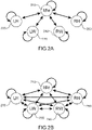
- the Fig. 2A represents a first example of a state diagram that can be used by the direct neural interface of the Fig. 1 .
- This state diagram models the movements of an exoskeleton, namely the movements of a left wrist (LW), a left hand (LH), a right wrist (RW) and a right hand ( HR).
- a resting state of the exoskeleton has been represented at 210, at 220 an active left wrist state, at 230 an active state of the left hand, at 240 an active state of the right wrist and at 250 an active state of the right hand .
- the transitions between states have been represented by arrows.
- This state diagram is based on a complete graph, in other words in which all the states are connected 2 by 2.
- This graph can become particularly complex when the number of states is high, for example when the articulations are numerous. In this case, learning is slow since each transition must be trained.
- the second predictive model i.e. the state classifier, can make detection errors leading to dysfunction of the exoskeleton.
- the exoskeleton has to perform complex tasks involving numerous states, the latency time for detecting a new error-free state can be relatively long, which is detrimental to its response speed and can prohibit rapid movements.
- An object of the present invention is therefore to propose a direct neural interface of the REW-MSLM type which does not have the aforementioned drawbacks, namely which allows complex movements implementing a plurality of effectors, while ensuring a short time. system response.
- the present invention is defined by one of a direct neural interface intended to receive a plurality of electrophysiological signals from a user acquired by means of a plurality of sensors and to supply control signals describing a trajectory to be carried out, said electrophysiological signals undergoing a pre-processing to obtain an observation tensor ( X t ) at each observation instant, in which the evolution of the observation tensor is modeled by a hierarchical HMM model, called H2M2, comprising a plurality of HMM sub-models organized according to a hierarchical tree structure, said tree structure comprising at its root a main model comprising a state of rest, each state of an HMM sub-model being either an internal state with which is associated a lower-level HMM sub-model in the tree, or a production state, said interface using a mixture of experts, each expert ( E s ) being associated with a production state and being defined by a multilinear predictive model, the predictions of each expert being combined by means of mixing coefficients ( ⁇ s,t
- Said tree structure comprises for example a right lateral state and a left lateral state corresponding respectively to the right part and to the left part of the body of the user, a first branch of the tree being associated with the right lateral state and a second branch of the tree being associated with the left lateral state
- B s and b s are respectively the tensors of the prediction coefficients and the prediction biases of the multilinear predictive model defining the expert associated with the production state s and ⁇ s,t is a characteristic mixing coefficient of the probability d occupation of production state s at time t.
- each of the experts, E s is trained according to a REW-NPLS regression method, on a sub-sequence of the observation tensor and the setpoint command tensor, corresponding to the state s ⁇ S production
- the mixing coefficients of the various experts can be estimated by means of a REW-NPLS regression method.
- At least some of the HMM sub-models of the tree structure are semi-Markovian.
- B s and b s are respectively the tensors of the prediction coefficients and the prediction biases of the multilinear predictive model defining the expert associated with the production state s
- ⁇ s,t is a vector whose elements are the respective probabilities ⁇ s,t that the production states are active
- ⁇ you issue is a vector giving the emission probabilities of the different production states and ⁇ is the Hadamard product.
- the probability of transition between a starting state and an arrival state of a semi-Markovian HMM sub-model is chosen all the higher as the duration of occupation of the starting state is greater.
- the transition probabilities between states of a semi-Markov HMM sub-model evolve over time according to a law parameterized by a plurality of temporal evolution parameters, said temporal evolution parameters being estimated in a supervised calibration phase during which the user receives instructions at a predetermined rate to perform one or more movements in a repetitive manner, the duration of occupation of each state of the semi-Markovian HMM sub-model being recorded over time.
- the transition probabilities between states of a semi-Markovian HMM sub-model evolve over time according to a law parameterized by a plurality of temporal evolution parameters, said temporal evolution parameters being estimated, in a calibration phase semi-supervised and/or an operational phase, from the observation tensor, the duration of occupation of each state of the semi-Markovian HMM sub-model being recorded over time.
- the electrophysiological signals are ECoG signals and the control signals are intended to control the actuators of an exoskeleton.
- the state classifier giving the probability of occupation of each state of the HMM model, uses a second predictive model and is also trained, during a calibration phase, by means of a REW-NPLS regression method.
- a first idea underlying the present invention is to use a hidden state automaton based on a hierarchical Markovian model, called HHMM ( Hierarchical Hidden Markov Model ) or more simply H2M2, organized according to a tree structure starting from a root common corresponding to the idle state.
- the tree of hidden states may in particular comprise a first branch corresponding to the right part of the user's body and a second branch corresponding to the left part of his body, the two branches coming from the common root.
- Other tree structures may be envisaged by those skilled in the art without departing from the scope of the present invention.
- the tree of hidden states could comprise a first branch corresponding to the right hand (dividing itself into sub-states corresponding to its position, its rotation, its open/closed character), a second branch (with the same division), and a third branch dividing itself into a first sub-state corresponding to the right leg and a sub-state corresponding to the left leg.
- the Fig. 3A schematically represents an example of the architecture of a hierarchical Markovian model with hidden states (H2M2) that can be used by a direct neural interface according to a first embodiment of the invention.
- H2M2 hierarchical Markovian model with hidden states
- This model includes a main HMM model, 310, called the rank 1 model, and two HMM sub-models, also called rank 2 models, a 320-R sub-model, being associated with the right part of the body and a sub-model. model, 320-L, being associated with the left part.
- the master model includes a resting state, 311, a first internal state corresponding to right body motion, 312-R, and a second internal state, 312-L, corresponding to left body motion. of the user.
- Each internal state is associated with a lateral HMM sub-model: thus, the 320-R sub-model is associated with the 312-R state and the 320-L sub-model is associated with the 312-L state of the major.
- the sub-model 320-R here comprises a first state 321-R associated with the right wrist and a second state 322-R associated with the right hand.
- the sub-model 320-L here comprises a first state, 321-L, associated with the left wrist, and a second state 322-L associated with the left hand.
- each state of the H2M2 model can be either an internal state or a production state.
- Each internal state of a rank d model is associated with an HMM sub-model of rank d +1, and each production state generates an observation with a given emission probability.
- the H2M2 model has a tree structure that can describe, for example, the hierarchical dependence of the joints of an exoskeleton.
- the Fig. 3B represents an example of a state diagram of an H2M2 model that can be used in the context of the present invention.
- the state s 1,1,1 corresponds to the state of rest
- the state s 2,1,1 is an internal state corresponding to the left part of the body
- the state s 3,1,1 is a state internal corresponding to its right side.
- the state s 2,1,1 is associated with a rank 2 HMM sub-model comprising two production states, s 1,1,2 , s 2,1,2 .
- a rank 2 HMM sub-model comprising two production states, s 1,1,2 , s 2,1,2 .
- s 3,1,1 is associated an HMM sub-model of rank 2, comprising two production states s 1,2,2 , s 2,2,2 .
- the states of the H2M2 model can be denoted in the indexed form s e,h,d where d is an index giving the rank (or level) of the state in the tree structure (or, equivalently, the rank of the HMM sub-model to which it belongs in the tree structure), h is the index of the sub-model in the level in question, and e is an index indexing the state in the sub-model.
- the sub-models are denoted in the form HMM h,d where d indicates the hierarchical level at which the model is located in the tree structure, and h is the index of the sub-model in the level.
- the tree structure is thus organized into levels or layers, indexed by the index d .
- the initial probability of occupation of each state s e,h,d of the HMM sub-model h,d is denoted ⁇ e,h,d .
- X _ 1 : you where card ( Z t ) is the cardinal of the set Z t and where we took for convention ⁇ 0 ( z t ) z t .
- the weighting coefficients ( gating coefficients), ⁇ s,t of the estimates provided by the various experts are calculated by means of a REW-NPLS regression method adapted to discrete decoding as described below.
- these weighting coefficients are updated from the training data set ( X u , Z u ), where X u is the input tensor of dimension ⁇ L ⁇ I 1 ⁇ ... ⁇ I n and Z u ⁇ 0,1 ⁇ K ⁇ L is the binary matrix, as defined in the introductory part. It is recalled that ⁇ L is the number of successive intervening instants taken into account in the calibration phase.
- these forgetting coefficients can be chosen to be identical or decreasing with the hierarchical level d (thus a deep model, that is to say close to the root, is updated more slowly than a model less deep).
- E h,d is the number of states of the HMM sub-model h,d and v I , I h , a is the number of transitions from state i to state j during the calibration phase u . It should be noted that this update does not only affect production states but also internal states.
- z t ) for the different production states are calculated by means of Bayes' rule, from the posterior conditional probabilities p ( ⁇ j ( z t )
- X _ you ⁇ I 0 card Z you
- the predictive module of the variable z t taking its values in S prod , is trained in a supervised manner in each calibration phase u according to the same principle as the predictive model of each expert.
- the REW-NPLS algorithm selects the hyperparameter f opt and the associated multilinear models, i.e.
- weighting coefficient ⁇ s,t expresses the probability that the production state s is active given the observed sequence (history of the observation tensor), X 1: t .
- X _ 1 : you where s e,h,d - j , j 0,..., d describe the states along the path leading to s .
- a second idea underlying the invention is to use in the H2M2 model, no longer Markovian sub-models HMM h,d but semi-Markovian sub-models or HSMM (Hidden Semi Markovian Model), noted for this reason HSMM h,d .
- the hierarchical model thus constructed is then denoted H2SM2.
- a semi-Markovian model is a Markovian model in which the transition probabilities between states are no longer constant but time-dependent. Specifically, the transition probability, has e , I h , , between a departure state s e,h,d and an arrival state s i,h,d of an HSMM sub-model h,d is an increasing function of the time spent in the departure state.
- I h , has 0 + 1 ⁇ has 0 tanh ⁇ e h , where 0 ⁇ a 0 ⁇ 1 is the transition probability at the initial instant and ⁇ e h , is the occupation time of the starting state.
- I h , has ⁇ 1 ⁇ exp ⁇ ⁇ e h , / T where a ⁇ is the transition probability for infinite time.
- I h , 1 2 1 ⁇ erf ⁇ e h , ⁇ ⁇ e h , ⁇ e h , 2 where ⁇ e h , is an average transition time, ⁇ e h , a standard deviation and erf(.) is the Gaussian error function.
- H2SM2 model could be semi-Markovian, HSMM h,d , the others being simply Markov.
- certain transitions between states may have a constant probability over time, the others depending on time as indicated above.
- ⁇ s,t is a vector of size K (number of states of the model) whose elements are the respective probabilities ⁇ s,t that the states are active
- ⁇ you issue is a vector of size K giving the emission probabilities of the different states
- ⁇ is the Hadamard product.
- the learning of the H2SM2 model differs from that of the H2M2 model in that the time evolution parameters of the transitions between states (e.g. ⁇ e h , , ⁇ e h , , a ⁇ , a 0 ) must be estimated.
- This learning can be performed in a calibration phase in supervised or semi-supervised mode.
- the user receives cadence instructions to perform one or more movements in a repetitive manner (or imagine these movements when the user has motor disabilities), if necessary at different speeds.
- the rate is provided to the user in the form of external stimuli (visual or sound for example).
- the updating of the parameters of the model is not limited to the calibration phase but continues in the operational phase.
- the rate or more generally the information relating to the temporal transitions between states is supplied by the output of the decoding.
- the variant in semi-supervised learning mode operates in the same way as in the variant in supervised mode, except that the rate information is provided by the decoder itself.
- the user may be asked to perform different movements repeatedly (walking for example) at different speeds, or even to think about these movements when the user has a motor disability.
- the temporal evolution parameters of the transition probabilities are estimated and updated from the respective durations of the states predicted by the H2SM2 model.
- Y _ ⁇ you ⁇ s ⁇ S production ⁇ SM s , you B _ s X _ you + b _ s
- Y SM st , s ⁇ S prod are the weighting coefficients of the different production states of the H2SM2 model, ie the respective probabilities of occupation of these states over time.
- the Fig. 4 schematically represents a direct neural interface using a mixture of experts controlled by a hierarchical (semi) Markovian model with hidden states according to a first (resp. a second) embodiment of the invention.
- the BCI interface, 400 involves, on the one hand, a hidden state automaton, 440, obeying a hierarchical Markovian (H2M2) or semi-Markovian (H2SM2) model and, on the other hand, a plurality of experts , 420, each estimator (or expert) being associated with a production state of the model H2(S)M2.
- H2M2 hierarchical Markovian
- H2SM2 semi-Markovian
- the electrophysiological signals from the sensors 405 are sampled and gathered in data blocks, each block corresponding to a sliding observation window defined by an observation instant at which the window in question starts.
- the signals undergo a pre-processing in the pre-processing module 410, comprising in particular a time-frequency analysis (decomposition into wavelets on the observation windows, for example), to provide an observation tensor, X t , at each instant of observation t.
- the estimates of the various experts are weighted at each instant of observation by weighting coefficients, ⁇ s,t ⁇ SM st , s ⁇ S prod and combined in the combining module 430 to provide an estimate of the control tensor according to expression (12) or (14).
- the weighting coefficients give at each instant the probabilities of occupation of the various states of the model 440, are estimated at each instant by means of a REW-NPLS regression in the estimation module 450.
- the parameters of this regression are determined in a calibration phase. If necessary, the lifetimes of the semi-Markov states are also estimated in this calibration phase in a supervised or semi-supervised way.
- the estimation of the lifetimes of the semi-Markov states can extend beyond the calibration phase, during the operational phase.
- the parameters ( B s , b s ) of the multilinear estimators associated with the different production states are determined on calibration sub-sequences associated with these states by means of a REW-NPLS regression, in a manner known to man of career.
Abstract
La présente invention concerne une interface neuronale directe destinée à estimer un tenseur de commande à partir d'un tenseur d'observation obtenu au moyen d'un pré-traitement des signaux électrophysiologiques d'un utilisateur. L'évolution du tenseur d'observation dans le temps est modélisée par un modèle H2M2, comprenant une pluralité de sous-modèles HMM organisés selon une arborescence hiérarchique. Ladite arborescence comporte à sa racine un sous-modèle HMM principal comprenant un état de repos dont sont issus différentes branches, par exemple une première branche de l'arborescence associée à un état latéral droit et une seconde branche de l'arborescence associée à un état latéral gauche. L'interface neuronale directe utilise un mélange d'experts, chaque expert étant associé à un état de production du modèle H2M2, chaque expert (E<sub>k</sub>) étant défini par un modèle prédictif multilinéaire, le tenseur de commande étant estimé au moyen d'une combinaison des prédictions des différents experts. Selon une variante, au moins certains des sous-modèles de l'arborescence sont semi-markoviens.The present invention relates to a direct neural interface intended to estimate a command tensor from an observation tensor obtained by means of a pre-processing of the electrophysiological signals of a user. The evolution of the observation tensor over time is modeled by an H2M2 model, comprising a plurality of HMM sub-models organized according to a hierarchical tree structure. Said tree structure comprises at its root a main HMM sub-model comprising a rest state from which various branches originate, for example a first branch of the tree structure associated with a right lateral state and a second branch of the tree structure associated with a left side. The direct neural interface uses a mixture of experts, each expert being associated with a production state of the H2M2 model, each expert (E<sub>k</sub>) being defined by a multilinear predictive model, the command tensor being estimated by means of a combination of the predictions of the different experts. According to a variant, at least some of the sub-models of the tree structure are semi-Markovian.
Description
La présente invention concerne le domaine des interfaces neuronales directes encore dénommées BCI (Brain Computer Interface) ou BMI (Brain Machine Interface). Elle trouve notamment à s'appliquer à la commande neuronale directe d'une machine, telle qu'un exosquelette ou un ordinateur.The present invention relates to the field of direct neuronal interfaces also called BCI ( Brain Computer Interface ) or BMI ( Brain Machine Interface ) . It finds particular application in the direct neural control of a machine, such as an exoskeleton or a computer.
Les interfaces neuronales directes utilisent les signaux électro-physiologiques émis par le cortex cérébral pour élaborer un signal de commande. Ces interfaces neuronales ont fait l'objet de nombreuses recherches notamment dans le but de restaurer une fonction motrice à un sujet paraplégique ou tétraplégique à l'aide d'une prothèse ou d'une orthèse motorisée.Direct neuronal interfaces use the electrophysiological signals emitted by the cerebral cortex to elaborate a control signal. These neuronal interfaces have been the subject of much research, in particular with the aim of restoring a motor function to a paraplegic or quadriplegic subject using a motorized prosthesis or orthosis.
Les interfaces neuronales peuvent être de nature invasive ou non invasive. Les interfaces neuronales invasives utilisent des électrodes intracorticales (c'est-à-dire implantées dans le cortex) ou des électrodes corticales (disposées à la surface du cortex) recueillant dans ce dernier cas des signaux électrocorticographiques (ECoG). Les interfaces neuronales non invasives utilisent des électrodes placées sur le cuir chevelu pour recueillir des signaux électroencéphalographiques (EEG). D'autres types de capteurs ont été également envisagés comme des capteurs magnétiques mesurant les champs magnétiques induits par l'activité électrique des neurones du cerveau. On parle alors de signaux magnétoencéphalographiques (MEG).Neural interfaces can be invasive or non-invasive in nature. Invasive neuronal interfaces use intracortical electrodes (that is to say implanted in the cortex) or cortical electrodes (arranged on the surface of the cortex) collecting in the latter case electrocorticographic signals (ECoG). Non-invasive neural interfaces use electrodes placed on the scalp to collect electroencephalographic (EEG) signals. Other types of sensors have also been envisaged, such as magnetic sensors measuring the magnetic fields induced by the electrical activity of brain neurons. These are called magnetoencephalographic (MEG) signals.
Les interfaces neuronales directes utilisent avantageusement des signaux de type ECoG, présentant l'avantage d'un bon compromis entre biocompatibilité (matrice d'électrodes implantées à la surface du cortex) et qualité des signaux recueillis.Direct neuronal interfaces advantageously use signals of the ECoG type, presenting the advantage of a good compromise between biocompatibility (matrix of electrodes implanted on the surface of the cortex) and quality of the signals collected.
Les signaux ECoG ainsi mesurés doivent être traités afin d'estimer la trajectoire du mouvement désiré par le sujet et en déduire les signaux de commande de l'ordinateur ou de la machine. Par exemple, lorsqu'il s'agit de commander un exosquelette, l'interface BCI estime la trajectoire du mouvement désiré à partir des signaux électro-physiologiques mesurés et en déduit les signaux de contrôle permettant à l'exosquelette de reproduire la trajectoire en question. De manière similaire, lorsqu'il s'agit de commander un ordinateur, l'interface BCI estime par exemple la trajectoire souhaitée d'un pointeur ou d'un curseur à partir des signaux électro-physiologiques et en déduit les signaux de commande du curseur/pointeur.The ECoG signals thus measured must be processed in order to estimate the trajectory of the movement desired by the subject and to deduce therefrom the command signals of the computer or of the machine. For example, when it comes to controlling an exoskeleton, the BCI interface estimates the trajectory of the desired movement from the measured electro-physiological signals and deduces the control signals allowing the exoskeleton to reproduce the trajectory in question. . Similarly, when it comes to controlling a computer, the BCI interface estimates for example the desired trajectory of a pointer or a cursor from the electro-physiological signals and deduces the cursor control signals. /pointer.
L'estimation de trajectoire, et plus précisément celle des paramètres cinématiques (position, vitesse, accélération), est encore dénommée décodage neuronal dans la littérature. Le décodage neuronal permet notamment de commander un mouvement (d'une prothèse ou d'un curseur) à partir de signaux ECoG.The trajectory estimation, and more precisely that of the kinematic parameters (position, speed, acceleration), is also called neural decoding in the literature. Neural decoding notably makes it possible to control a movement (of a prosthesis or of a cursor) from ECoG signals.
Lorsque les signaux ECoG sont acquis en continu, l'une des principales difficultés du décodage réside dans le caractère asynchrone de la commande, autrement dit dans la discrimination des phases pendant lesquelles le sujet commande effectivement un mouvement (périodes actives) des phases où il n'en commande pas (périodes de repos).When ECoG signals are acquired continuously, one of the main difficulties in decoding lies in the asynchronous nature of the command, in other words in the discrimination of the phases during which the subject actually commands a movement (active periods) from the phases where he does not not on order (periods of rest).
Pour contourner cette difficulté, des interfaces neuronales directes, dites synchrones, ne donnent la possibilité de commander un mouvement que pendant des fenêtres temporelles bien déterminées (par exemple des intervalles de temps se succédant périodiquement), signalées au sujet par un indice extérieur. Le sujet ne peut alors commander le mouvement que pendant ces fenêtres temporelles, ce qui s'avère prohibitif dans la plupart des applications pratiques.To circumvent this difficulty, direct neural interfaces, called synchronous, only give the possibility of controlling a movement during well-defined time windows (for example time intervals which follow one another periodically), signaled to the subject by an external cue. The subject can then only control the movement during these time windows, which proves to be prohibitive in most practical applications.
Plus récemment, des interfaces neuronales directes à décodage continu ont été proposées dans la littérature. L'article de
Une autre approche a été proposée dans l'article de
Enfin, les interfaces neuronales directes précitées ont été développées pour décoder le mouvement d'un seul membre d'un sujet. Elles ne sont donc pas adaptées à la commande d'un exosquelette à plusieurs membres, notamment pour un sujet tétraplégique, paraplégique ou hémiplégique, ce qui limite sensiblement leur champ d'application.Finally, the aforementioned direct neural interfaces have been developed to decode the movement of a single limb of a subject. They are therefore not suitable for controlling an exoskeleton with several limbs, in particular for a quadriplegic, paraplegic or hemiplegic subject, which significantly limits their field of application.
Il a été proposé dans la demande publiée sous le numéro
On a représenté schématiquement en
Cette interface, 100, fait intervenir, d'une part, un automate à états cachés, 140, pouvant prendre K états possibles et, d'autre part, une pluralité K d'estimateurs, 120, chaque estimateur (ou expert) étant associé à un état caché.This interface, 100, involves, on the one hand, a hidden state automaton, 140, able to take K possible states and, on the other hand, a plurality K of estimators, 120, each estimator (or expert) being associated to a hidden state.
Les estimations des différents experts sont combinées dans un module de combinaison (gating network), 130, pour donner une estimation, ŷ(t) de la variable à expliquer, y(t), ici les paramètres cinématiques du mouvement, à partir de l'observation x(t) représentant les caractéristiques des signaux neuronaux à l'instant t, captés au moyen des électrodes 105. La séquence des observations x[1:t]={x(1), x(2),..., x(t)} est modélisée par un processus markovien sous-jacent, de premier ordre, à émission continue.The estimates of the various experts are combined in a combination module ( gating network ), 130, to give an estimate, ŷ ( t ) of the variable to be explained, y(t), here the kinematic parameters of the movement, from l observation x(t) representing the characteristics of the neural signals at time t, picked up by means of the
Si la variable d'entrée x(t) est de dimension M et la réponse y(t) de dimension N, et si les modèles prédictifs des différents experts Ek , sont choisis linéaires, autrement dit Ek (x(t)) = β k x(t) où β k est une matrice de taille N × M, l'estimation par mélange d'experts s'exprime comme suit : 

Comme indiqué dans la demande précitée, les paramètres du modèle HMM, c'est-à-dire les probabilités de transition entre états cachés, et les matrices β k peuvent être estimés lors d'une phase de calibration, au moyen d'une méthode d'estimation supervisée. Dans ce cas, l'automate HMM et les K experts sont entraînés indépendamment les uns des autres. En particulier, chaque expert Ek peut être entrainé sur une sous-séquence d'observations correspondant à l'état k , la matrice β k du modèle prédictif étant alors estimée au moyen d'une régression PLS (Partial Least Squares) linéaire à partir de cette sous-séquence.As indicated in the aforementioned application, the parameters of the HMM model, that is to say the probabilities of transition between hidden states, and the matrices β k can be estimated during a calibration phase, by means of a method of supervised estimation. In this case, the automaton HMM and the K experts are trained independently of each other. In particular, each expert E k can be trained on a sub-sequence of observations corresponding to state k , the matrix β k of the model predictive being then estimated by means of a linear PLS ( Partial Least Squares) regression from this sub-sequence.
De manière plus générale, la relation linéaire (1) peut être étendue à une relation multilinéaire. La variable d'entrée peut être alors représentée sous forme tensorielle ![]()
![]()
Les modes du tenseur d'entrée peuvent être par exemple le temps (nombre d'échantillons dans le temps), la fréquence (nombre de bandes spectrales d'analyse), l'espace (nombre d'électrodes). De même, la réponse peut être représentée sous forme tensorielle ![]()
![]()
Les tenseurs des modèles prédictifs des différents experts peuvent alors être estimés par une méthode PLS multivariée ou NPLS (N-way PLS) comme décrit dans la demande publiée sous le numéro
Quels que soient les modèles prédictifs (PLS ou NPLS) des différents experts, on a pu constater qu'en raison de l'absence de stationnarité des signaux dans le cerveau humain, la durée de validité de ces modèles était relativement limitée. Il est par conséquent nécessaire de les mettre à jour régulièrement en procédant à de nouvelles phases de calibration. Or, chaque nouvelle phase de calibration nécessite de traiter une quantité de données très importante, combinant les données des calibrations antérieures et celles de la nouvelle calibration, et ce pour les différents experts. La durée de la mise à jour est alors souvent telle qu'elle requiert une interruption du fonctionnement de l'interface neuronale directe (calibration dite off-line). Il a été ainsi proposé dans la demande
Il a été proposé dans la demande
Une telle interface neuronale directe, désignée dans la littérature par l'acronyme REW-MSLM (Recursive Exponentially Weighted Markov Switching Multi-Linear Model), hérite, d'une part, des caractéristiques d'un décodage REW-NPLS et, d'autre part, de celles d'un mélange d'experts commandé par un modèle HMM comme décrit en relation avec la
Une interface neuronale directe REW-MSLM est brièvement décrite ci-après. Celle-ci fournit un tenseur de commande à partir d'un tenseur d'observation.A direct REW-MSLM neural interface is briefly described below. This provides a control tensor from an observation tensor.
Le tenseur représentant la variable d'entrée, dit tenseur d'entrée ou tenseur d'observation, est d'ordre n+1, le premier mode étant celui relatif aux instants d'observation (epochs). Le tenseur d'entrée (ou tenseur d'observation) est noté X et est de dimension N×I 1×...×In. The tensor representing the input variable, called input tensor or observation tensor, is of order n +1, the first mode being that relating to observation times (epochs). The input tensor (or observation tensor) is denoted X and has dimension N × I 1 × ... × I n .
De la même façon, la trajectoire du mouvement imaginé, observé ou réalisé est décrite par un tenseur de sortie (ou tenseur de commande), d'ordre m + 1, noté Y, de dimension N×J 1×...×Jm, dont le premier mode correspond aux instants successifs auxquels s'appliqueront les commandes, les autres modes correspondant aux commandes de différents effecteurs ou aux différents degrés de liberté d'un robot multi-axe.In the same way, the trajectory of the imagined, observed or realized movement is described by an output tensor (or control tensor), of order m + 1, denoted Y, of dimension N × J 1 ×...× J m , the first mode of which corresponds to the successive instants to which the commands will be applied, the other modes corresponding to the commands of various effectors or to the various degrees of freedom of a multi-axis robot.
Le tenseur de sortie fournit N blocs consécutifs de données de commande, chacun des blocs permettant de générer les signaux de commande relatifs aux différents effecteurs ou degrés de liberté. Ainsi, l'homme du métier comprendra que la dimension de chaque bloc de données pourra dépendre du cas d'usage envisagé et notamment du nombre de degrés de liberté de l'effecteur.The output tensor provides N consecutive blocks of control data, each of the blocks making it possible to generate the control signals relating to the different effectors or degrees of freedom. Thus, those skilled in the art will understand that the dimension of each data block may depend on the case of use envisaged and in particular on the number of degrees of freedom of the effector.
On note dans la suite X t le tenseur d'observation à l'instant t . Ce tenseur est par conséquent d'ordre n et de dimension I 1×...×In. Il prend ses valeurs dans un espace ![]()
![]()
![]()
![]()
![]()
![]()
On suppose que l'espace X est formé par l'union d'une pluralité K de régions, non nécessairement disjointes. Autrement dit, 
L'interface neuronale directe REW-MSLM utilise un mélange d'experts, chaque expert Ek opérant sur la région élémentaire Xk de l'espace des caractéristiques d'entrée et étant capable de prédire le tenseur de commande Y t à l'instant t à partir du tenseur d'observation, X t , lorsque ce dernier appartient à Xk . Autrement dit, à chaque région Xk correspond un modèle de prédiction du tenseur de commande Y t à partir du tenseur d'observation X t . Un expert Ek peut être ainsi considéré comme une application multilinéaire de Xk dans Y .The direct neural interface REW-MSLM uses a mixture of experts, each expert E k operating on the elementary region X k of the input feature space and being able to predict the control tensor Y t at the instant t from the observation tensor, X t , when the latter belongs to X k . In other words, to each region X k corresponds a prediction model of the control tensor Y t from the observation tensor X t . An expert E k can thus be considered as a multilinear map from X k to Y .
On suppose par ailleurs que chaque expert Ek est associé à un état caché k d'un modèle Markovien du premier ordre (HMM). Les différents experts sont combinés à l'aide de coefficients de combinaison dépendant de l'état caché au moment de la prédiction. En définitive, à partir d'un tenseur d'entrée (ou d'observation) X t , l'interface neuronale estime le tenseur de sortie (ou de commande) Y t , au moyen de : 
![]()
![]()
![]()
![]()
L'ensemble des coefficients et des biais de prédiction, dénommés collectivement paramètres de prédiction des différents experts est désigné par θ e = {( β k ,δ k )|k= 1,..,K}. L'ensemble de paramètres relatifs à la combinaison des différents experts (incluant les paramètres du modèle HMM sous-jacent) est désigné quant à lui par θ g = {A , {dk |k=1,..,K},π } où A est la matrice de transition entre états, de taille K × K , c'est-à-dire la matrice dont les éléments aij (indépendants du temps par hypothèse du modèle HMM) sont définis par aij = p(zt = j|z t-1 = i) où zt représente l'état du modèle à l'instant t et z t-1 représente l'état du modèle à l'instant précédent; {dk |k = 1,..,K} les paramètres permettant de déterminer la probabilité conditionnelle d'observer le tenseur d'entrée X t connaissant l'état zt =k , et π est un vecteur de taille K donnant les probabilités d'occupation des différents états à l'instant initial, autrement dit πi = p(zt = i) t=0 . The set of prediction coefficients and biases, collectively referred to as the prediction parameters of the different experts, is denoted by θ e = {( β k , δ k )| k = 1,.., K }. The set of parameters relating to the combination of the different experts (including the parameters of the underlying HMM model) is designated by θ g = { A , { d k | k =1,.., K } , π } where A is the transition matrix between states, of size K × K , i.e. the matrix whose elements a ij (independent of time by assumption of the model HMM) are defined by a ij = p ( z t = j | z t -1 = i ) where z t represents the state of the model at time t and z t- 1 represents the state of the model at previous moment; { d k | k = 1,.., K } the parameters allowing to determine the conditional probability of observing the input tensor X t knowing the state z t = k , and π is a vector of size K giving the probabilities of occupation of the different states at the initial instant, in other words π i = p ( z t = i ) t =0 .
Le décodeur REW-MSLM est entrainé pendant des phases de calibration indicées par l'indice u , chaque phase de calibration faisant intervenir une pluralité ΔL d'instants successifs issus de la séquence d'observation. On note X u le tenseur de dimension ΔL × I 1 ×...× In regroupant les tenseurs d'entrée pendant la phase de calibration u, et Z u ∈{0,1} K×ΔL la matrice binaire donnant, à chaque instant, l'état latent du modèle HMM (la matrice possédant un seul élément égal à 1 par colonne indiquant l'état actif parmi les K états possibles).The REW-MSLM decoder is driven during calibration phases indexed by the index u , each calibration phase involving a plurality ΔL of successive instants from the observation sequence. We note X u the tensor of dimension Δ L × I 1 ×...× I n grouping the input tensors during the calibration phase u , and Z u ∈{0.1} K ×Δ L the binary matrix giving , at each instant, the latent state of the HMM model (the matrix having a single element equal to 1 per column indicating the active state among the K possible states).
L'interface neuronale directe REW-MSLM permet de contrôler plusieurs effecteurs agissant sur différentes articulations d'un exosquelette, un état pouvant être associé à une articulation par exemple. En outre, elle permet de garantir la stabilité d'un état au repos (idle state) prolongé et un contrôle asynchrone des effecteurs.The direct neural interface REW-MSLM allows control of multiple effectors acting on different joints of an exoskeleton, a state that can be associated with a joint for example. In addition, it makes it possible to guarantee the stability of a prolonged idle state and an asynchronous control of the effectors.
La
Ce diagramme d'états modélise les mouvements d'un exosquelette, à savoir les mouvements d'un poignet gauche (LW), d'une main gauche (LH), d'un poignet droit (RW) et d'une main droite (RH).This state diagram models the movements of an exoskeleton, namely the movements of a left wrist (LW), a left hand (LH), a right wrist (RW) and a right hand ( HR).
On a représenté en 210 un état de repos de l'exosquelette, en 220 un état actif poignet gauche, en 230 un état actif de la main gauche, en 240 un état actif du poignet droit et en 250 un état actif de la main droite. Les transitions entre états ont été représentées par des flèches.A resting state of the exoskeleton has been represented at 210, at 220 an active left wrist state, at 230 an active state of the left hand, at 240 an active state of the right wrist and at 250 an active state of the right hand . The transitions between states have been represented by arrows.
On note que dans un tel diagramme d'états, pour passer d'un mouvement du poignet gauche à celui de la main gauche par exemple, il faut passer par l'état de repos. Ce diagramme d'états est très simple et favorise excessivement l'état de repos au détriment des états actifs. S'il présente l'avantage de réduire le taux de mauvaise détection des états actifs les plus rares lorsque le nombre d'états est élevé, il ne permet pas d'effectuer des mouvements fluides.It is noted that in such a state diagram, to pass from a movement of the left wrist to that of the left hand for example, it is necessary to pass through the state of rest. This state diagram is very simple and excessively favors the resting state to the detriment of the active states. If it has the advantage of reducing the bad detection rate of the rarest active states when the number of states is high, it does not allow fluid movements to be performed.
En effet, le passage obligé par l'état de repos conduit à des temps de latence importants entre états actifs, ce qui pénalise la réactivité de la réponse aux signaux électrophysiologiques.Indeed, the obligatory passage through the resting state leads to significant latency times between active states, which penalizes the reactivity of the response to electrophysiological signals.
Une solution possible pour accroître la réactivité de cette réponse est d'utiliser un diagramme d'états tel que celui représenté en
Les éléments portant les mêmes numéros de référence sont identiques à ceux de la
Ce diagramme d'états est basé sur un graphe complet, autrement dit dans lequel tous les états sont connectés 2 à 2. Ce graphe peut devenir particulièrement complexe lorsque le nombre d'états est élevé, par exemple lorsque les articulations sont nombreuses. Dans ce cas, l'apprentissage est lent étant donné que chaque transition doit être entrainée. En outre, le second modèle prédictif, c'est-à-dire le classificateur d'états, peut commettre des erreurs de détection conduisant à un dysfonctionnement de l'exosquelette. Enfin, lorsque l'exosquelette doit effectuer des tâches complexes mettant en jeu de nombreux états, le temps de latence pour détecter un nouvel état sans erreur peut être relativement long, ce qui est préjudiciable à sa vitesse de réponse et peut interdire des mouvements rapides.This state diagram is based on a complete graph, in other words in which all the states are connected 2 by 2. This graph can become particularly complex when the number of states is high, for example when the articulations are numerous. In this case, learning is slow since each transition must be trained. Furthermore, the second predictive model, i.e. the state classifier, can make detection errors leading to dysfunction of the exoskeleton. Finally, when the exoskeleton has to perform complex tasks involving numerous states, the latency time for detecting a new error-free state can be relatively long, which is detrimental to its response speed and can prohibit rapid movements.
Un but de la présente invention est par conséquent de proposer une interface neuronale directe de type REW-MSLM qui ne présente pas les inconvénients précités, à savoir qui autorise des mouvements complexes mettant en œuvre une pluralité d'effecteurs, tout en assurant un faible temps de réponse du système.An object of the present invention is therefore to propose a direct neural interface of the REW-MSLM type which does not have the aforementioned drawbacks, namely which allows complex movements implementing a plurality of effectors, while ensuring a short time. system response.
La présente invention est définie par une d'une interface neuronale directe destinée à recevoir une pluralité de signaux électrophysiologiques d'un usager acquis au moyen d'une pluralité de capteurs et à fournir des signaux de commande décrivant une trajectoire à réaliser, lesdits signaux électrophysiologiques subissant un prétraitement pour obtenir un tenseur d'observation ( X t ) en chaque instant d'observation, dans laquelle l'évolution du tenseur d'observation est modélisée par un modèle HMM hiérarchisé, dit H2M2, comprenant une pluralité de sous-modèles HMM organisés selon une arborescence hiérarchique, ladite arborescence comportant à sa racine un modèle principal comprenant un état de repos , chaque état d'un sous-modèle HMM étant soit un état interne auquel est associé un sous-modèle HMM de plus bas niveau dans l'arborescence, soit un état de production, ladite interface utilisant un mélange d'experts, chaque expert (Es ) étant associé à un état de production et étant défini par un modèle prédictif multilinéaire, les prédictions de chaque expert étant combinées au moyen de coefficients de mélange (γs,t, γSM
Ladite arborescence comporte par exemple un état latéral droit et un état latéral gauche correspondant respectivement à la partie droite et à la partie gauche du corps de l'usager, une première branche de l'arborescence étant associée à l'état latéral droit et une seconde branche de l'arborescence étant associée à l'état latéral gaucheSaid tree structure comprises for example a right lateral state and a left lateral state corresponding respectively to the right part and to the left part of the body of the user, a first branch of the tree being associated with the right lateral state and a second branch of the tree being associated with the left lateral state
Avantageusement, le tenseur de commande Y t est estimé à partir du tenseur d'observation X t au moyen de ![]()
![]()
Dans une phase de calibration, chacun des experts, Es , est entrainé selon une méthode de régression REW-NPLS, sur une sous-séquence du tenseur d'observation et du tenseur de commande de consigne, correspondant à l'état s ∈ Sprod. In a calibration phase, each of the experts, E s , is trained according to a REW-NPLS regression method, on a sub-sequence of the observation tensor and the setpoint command tensor, corresponding to the state s ∈ S production
Dans ladite phase de calibration, les coefficients de mélange des différents experts peuvent être estimés au moyen d'une méthode de régression REW-NPLS.In said calibration phase, the mixing coefficients of the various experts can be estimated by means of a REW-NPLS regression method.
Avantageusement, au moins certains des sous-modèles HMM de l'arborescence sont semi-markoviens.Advantageously, at least some of the HMM sub-models of the tree structure are semi-Markovian.
Dans ce cas, le tenseur de commande Y t peut être estimé à partir du tenseur d'observation X t au moyen de 
![]()
![]()
![]()
![]()
La probabilité de transition entre un état de départ et un état d'arrivée d'un sous-modèle HMM semi-markovien est choisie d'autant plus élevée que la durée d'occupation de l'état de départ est plus grande.The probability of transition between a starting state and an arrival state of a semi-Markovian HMM sub-model is chosen all the higher as the duration of occupation of the starting state is greater.
Avantageusement, les probabilités de transition entre états d'un sous-modèle HMM semi-markovien évoluent dans le temps selon une loi paramétrée par une pluralité de paramètres d'évolution temporelle, lesdits paramètres d'évolution temporelle étant estimés dans une phase de calibration supervisée pendant laquelle l'usager reçoit des instructions de cadence prédéterminée pour effectuer un ou des mouvement(s) de manière répétitive, la durée d'occupation de chaque état du sous-modèle HMM semi-markovien étant enregistrée au cours du temps.Advantageously, the transition probabilities between states of a semi-Markov HMM sub-model evolve over time according to a law parameterized by a plurality of temporal evolution parameters, said temporal evolution parameters being estimated in a supervised calibration phase during which the user receives instructions at a predetermined rate to perform one or more movements in a repetitive manner, the duration of occupation of each state of the semi-Markovian HMM sub-model being recorded over time.
Alternativement, les probabilités de transition entre états d'un sous-modèle HMM semi-markovien évoluent dans le temps selon une loi paramétrée par une pluralité de paramètres d'évolution temporelle, lesdits paramètres d'évolution temporelle étant estimés, dans une phase de calibration semi-supervisée et/ou une phase opérationnelle, à partir du tenseur d'observation, la durée d'occupation de chaque état du sous-modèle HMM semi-markovien étant enregistrée au cours du temps.Alternatively, the transition probabilities between states of a semi-Markovian HMM sub-model evolve over time according to a law parameterized by a plurality of temporal evolution parameters, said temporal evolution parameters being estimated, in a calibration phase semi-supervised and/or an operational phase, from the observation tensor, the duration of occupation of each state of the semi-Markovian HMM sub-model being recorded over time.
Dans un exemple de réalisation, les signaux électrophysiologiques sont des signaux ECoG et les signaux de commande sont destinés à commander les actuateurs d'un exosquelette.In an exemplary embodiment, the electrophysiological signals are ECoG signals and the control signals are intended to control the actuators of an exoskeleton.
D'autres caractéristiques et avantages de l'invention apparaîtront à la lecture d'un mode de réalisation préférentiel de l'invention, décrit en référence aux figures jointes parmi lesquelles :
- La
Fig. 1 , déjà décrite, représente de manière schématique une interface neuronale directe utilisant un mélange markovien d'experts, connue de l'état de la technique ; - La
Fig. 2A , déjà décrite, représente un premier exemple de diagramme d'états pouvant être utilisé par l'interface neuronale directe de laFig. 1 ; - La
Fig. 2B , déjà décrite, représente un second exemple de diagramme d'états pouvant être utilisé par l'interface neuronale directe de laFig. 1 ; - La
Fig. 3A représente l'architecture générale d'un modèle hiérarchique markovien à états cachés (H2M2) pouvant être utilisé par une interface neuronale directe selon un premier mode de réalisation de l'invention ; - La
Fig. 3B représente de manière schématique un exemple détaillé de diagramme d'états d'un modèle un modèle hiérarchique markovien à états cachés (H2M2) pouvant être utilisé par une interface neuronale directe selon un premier mode de réalisation de l'invention ; - La
Fig. 4 représente de manière schématique un interface neuronale directe utilisant un mélange d'experts contrôlé par un modèle hiérarchique (semi) markovien à états cachés selon un premier (resp. un second) mode de réalisation de l'invention.
- The
Fig. 1 , already described, schematically represents a direct neuronal interface using a Markov mixture of experts, known from the state of the art; - The
Fig. 2A , already described, represents a first example of a state diagram that can be used by the direct neural interface of theFig. 1 ; - The
Fig. 2B , already described, represents a second example of a state diagram that can be used by the direct neural interface of theFig. 1 ; - The
Fig. 3A represents the general architecture of a hierarchical Markovian model with hidden states (H2M2) that can be used by a direct neural interface according to a first embodiment of the invention; - The
Fig. 3B schematically represents a detailed example of a state diagram of a model a hierarchical Markovian model with hidden states (H2M2) that can be used by a direct neural interface according to a first embodiment of the invention; - The
Fig. 4 schematically represents a direct neural interface using a mixture of experts controlled by a hierarchical (semi) Markovian model with hidden states according to a first (resp. a second) embodiment of the invention.
On considérera dans la suite une interface neuronale directe de type REW-MSLM telle que décrit dans la partie introductive. On rappelle que cette interface utilise un automate à états cachés, basé sur modèle HMM, pouvant prendre K états possibles, ainsi qu'une pluralité d'experts Ek,k = 1,..., K, utilisant un premier modèle prédictif, chaque expert étant associé à un état caché. Chaque expert Ek est entrainé, dans une phase de calibration, selon une méthode de régression REW-NPLS, sur une sous-séquence du tenseur d'observation et du tenseur de commande de consigne, correspondant à l'état k. Le classificateur d'état, donnant la probabilité d'occupation de chaque état du modèle HMM, utilise un second modèle prédictif et est également entrainé, pendant une phase de calibration, au moyen d'une méthode de régression REW-NPLS.In what follows, a direct neuronal interface of the REW-MSLM type as described in the introductory part will be considered. It is recalled that this interface uses a hidden state automaton, based on the HMM model, which can take K possible states, as well as a plurality of experts E k ,k = 1,..., K, using a first predictive model, each expert being associated with a hidden state. Each expert E k is trained, in a calibration phase, according to a REW-NPLS regression method, on a sub-sequence of the observation tensor and of the setpoint command tensor, corresponding to the state k . The state classifier, giving the probability of occupation of each state of the HMM model, uses a second predictive model and is also trained, during a calibration phase, by means of a REW-NPLS regression method.
Une première idée à la base de la présente invention est d'utiliser un automate à états cachés basé sur un modèle markovien hiérarchisé, dénommé HHMM (Hierarchical Hidden Markov Model) ou plus simplement H2M2, organisé selon une structure arborescente à partir d'une racine commune correspondant à l'état de repos (idle state). L'arbre des états cachés pourra notamment comprendre une première branche correspondant à la partie droite du corps de l'usager et une seconde branche correspondant à la partie gauche de son corps, les deux branches étant issues de la racine commune. D'autres structures arborescentes pourront être envisagées par l'homme du métier sans sortir du cadre de la présente invention. Par exemple, l'arbre des états cachés pourra comporter une première branche correspondant à la main droite (se divisant elle-même en sous-états correspondant à sa position, sa rotation, son caractère ouvert/fermé), une seconde branche (avec la même division), et une troisième branche se divisant elle-même en un premier sous-état correspondant à la jambe droite et un sous état correspondant à la jambe gauche.A first idea underlying the present invention is to use a hidden state automaton based on a hierarchical Markovian model, called HHMM ( Hierarchical Hidden Markov Model ) or more simply H2M2, organized according to a tree structure starting from a root common corresponding to the idle state. The tree of hidden states may in particular comprise a first branch corresponding to the right part of the user's body and a second branch corresponding to the left part of his body, the two branches coming from the common root. Other tree structures may be envisaged by those skilled in the art without departing from the scope of the present invention. For example, the tree of hidden states could comprise a first branch corresponding to the right hand (dividing itself into sub-states corresponding to its position, its rotation, its open/closed character), a second branch (with the same division), and a third branch dividing itself into a first sub-state corresponding to the right leg and a sub-state corresponding to the left leg.
La
Ce modèle comprend un modèle HMM principal, 310, dit modèle de rang 1, et deux sous-modèles HMM, dits encore modèles de rang 2, un sous-modèle 320-R, étant associé à la partie droite du corps et un sous-modèle, 320-L, étant associé à la partie gauche. Le modèle principal comprend un état de repos, 311, un premier état interne correspondant à un mouvement de la partie droite du corps, 312-R, et un second état interne, 312-L, correspondant à un mouvement de la partie gauche du corps de l'usager. A chaque état interne est associé un sous-modèle HMM latéral : ainsi, le sous-modèle 320-R est associé à l'état 312-R et le sous-modèle 320-L est associé à l'état 312-L du modèle principal. Le sous-modèle 320-R comprend ici un premier état 321-R associé au poignet droit et un second état 322-R associé à la main droite. De même, le sous-modèle 320-L comprend ici un premier état, 321-L, associé au poignet gauche, et un second état 322-L associé à la main gauche. Lorsqu'un état du sous-modèle 320-R est actif, cela suppose que l'état interne, 312-R, du modèle principal l'est aussi. De manière similaire, lorsqu'un état du sous-modèle 320-L est actif, cela suppose que l'état interne, 312-L du modèle principal l'est aussi.This model includes a main HMM model, 310, called the
De manière générale, chaque état du modèle H2M2 peut être soit un état interne, soit un état de production. Chaque état interne d'un modèle de rang d est associé à un sous-modèle HMM de rang d +1, et chaque état de production génère une observation avec une probabilité d'émission donnée.Generally speaking, each state of the H2M2 model can be either an internal state or a production state. Each internal state of a rank d model is associated with an HMM sub-model of rank d +1, and each production state generates an observation with a given emission probability.
Ainsi, par exemple, l'état 322-R associé à la main droite peut être un état de production générant une observation soit un état interne associé à un sous-modèle de rang d = 3 comportant un état pour chaque doigt. Un état associé à un doigt peut être lui-même être associé à un sous-modèle de rang d = 4, comportant un état pour chaque phalange.Thus, for example, the state 322-R associated with the right hand can be a production state generating an observation or an internal state associated with a sub-model of rank d =3 comprising a state for each finger. A state associated with a finger can itself be associated with a sub-model of rank d =4, comprising a state for each phalanx.
On comprend ainsi que le modèle H2M2 présente une structure arborescente pouvant décrire, par exemple, la dépendance hiérarchique des articulations d'un exosquelette.It is thus understood that the H2M2 model has a tree structure that can describe, for example, the hierarchical dependence of the joints of an exoskeleton.
La
Dans le cas présent, il s'agit d'un modèle H2M2 à deux niveaux hiérarchiques. Le modèle HMM de rang 1 (h =1) comprend trois états notés respectivement s 1,1,1, s 2,1,1, s 3,1,1 . L'état s 1,1,1 correspond à l'état de repos, l'état s 2,1,1 est un état interne correspondant à la partie gauche du corps et l'état s 3,1,1 est un état interne correspondant à sa partie droite.In this case, it is an H2M2 model with two hierarchical levels. The HMM model of rank 1 ( h =1) comprises three states noted respectively s 1,1,1 , s 2,1,1 , s 3,1,1 . The state s 1,1,1 corresponds to the state of rest, the state s 2,1,1 is an internal state corresponding to the left part of the body and the state s 3,1,1 is a state internal corresponding to its right side.
A l'état s 2,1,1 est associé un sous-modèle HMM de rang 2 comprenant deux états de production, s 1,1,2, s 2,1,2. De même à l'état s 3,1,1 est associé un sous-modèle HMM de rang 2, comprenant deux états de productions s 1,2,2, s 2,2,2 .The state s 2,1,1 is associated with a
De manière générale, les états du modèle H2M2 pourront être notés sous la forme indexée se,h,d où d est un indice donnant le rang (ou le niveau) de l'état dans l'arborescence (ou, de manière équivalente, le rang du sous-modèle HMM auquel il appartient dans l'arborescence), h est l'indice du sous-modèle dans le niveau en question, et e est un indice indexant l'état dans le sous-modèle. Les sous-modèles sont quant à eux notés sous la forme HMMh,d où d indique le niveau hiérarchique auquel le modèle se situe dans l'arborescence, et h est l'indice du sous-modèle dans le niveau. L'arborescence est ainsi organisée en niveaux ou couches, indexé(e)s par l'indice d. Chaque sous-modèle HMMh,d est caractérisé par sa matrice de transition entre états ![]()
![]()
![]()
![]()
![]()
![]()
La probabilité initiale d'occupation de chaque état se,h,d du sous-modèle HMMh,d est notée πe,h,d. The initial probability of occupation of each state s e,h,d of the HMM sub-model h,d is denoted π e,h,d .
Enfin, l'ensemble des états de production du modèle H2M2 est noté Sprod et celui des états internes est noté Sint où S = Sprod ∪ Sint est l'ensemble des états du modèle. Si l'on note zt la variable indiquant l'état de production à l'instant t , X t le tenseur d'observation en cet instant, la probabilité d'émission de cet état n'est autre que p( X t |zt ).Finally, the set of production states of the H2M2 model is denoted S prod and that of the internal states is denoted S int where S = S prod ∪ S int is the set of states of the model. If we note z t the variable indicating the state of production at time t , X t the observation tensor at this time, the probability of emission of this state is none other than p ( X t | zt ).
On définit en outre, pour tout état actif, se,h,d de la couche d > 1 , ψ(se,h,d ) = s e',h',d-1 l'état actif appartenant à la couche précédente. Ainsi, pour un état de production zt à l'instant t, appartenant à la couche d, l'ensemble Zt = {zt,ψ (zt ),ψ 2 (zt ),...,ψd (zt )} définit un chemin d'états actifs dans l'arborescence du modèle H2M2 conduisant à l'état de production.We further define, for any active state, s e,h,d of the layer d > 1 , ψ ( s e,h,d ) = s e',h',d -1 the active state belonging to the previous layer. Thus, for a production state z t at time t, belonging to layer d, the set Z t = { z t ,ψ ( z t ), ψ 2 ( z t ),..., ψ d ( z t )} defines a path of active states in the H2M2 model tree leading to the production state.
La probabilité d'activation d'un état s de S à l'instant t est alors définie par : 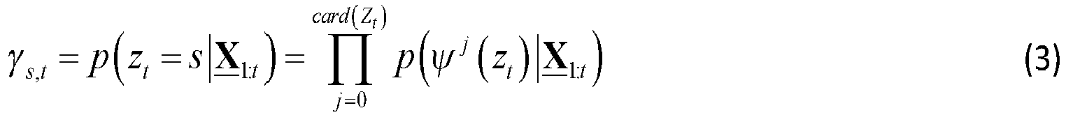
Les coefficients de pondération (gating coefficients), γs,t des estimations fournies par les différents experts sont calculés au moyen d'une méthode de régression REW-NPLS adaptée au décodage discret comme décrit plus loin.The weighting coefficients ( gating coefficients), γ s,t of the estimates provided by the various experts are calculated by means of a REW-NPLS regression method adapted to discrete decoding as described below.
Plus précisément, à chaque phase de calibration u, ces coefficients de pondération sont mis à jour à partir de l'ensemble de données d'apprentissage ( X u ,Z u ), où X u est le tenseur d'entrée de dimension ΔL×I 1×...×In et Z u ∈{0,1} K×ΔL est la matrice binaire, tels que définis dans la partie introductive. On rappelle que ΔL est le nombre d'instants successifs intervenant pris en compte dans la phase de calibration.More precisely, at each calibration phase u , these weighting coefficients are updated from the training data set ( X u , Z u ), where X u is the input tensor of dimension Δ L × I 1 × ... × I n and Z u ∈{0,1} K ×Δ L is the binary matrix, as defined in the introductory part. It is recalled that ΔL is the number of successive intervening instants taken into account in the calibration phase.
Les éléments de chacune des matrices de transition A h,d des modèles HMMh,d sont mis à jour de la manière suivante : 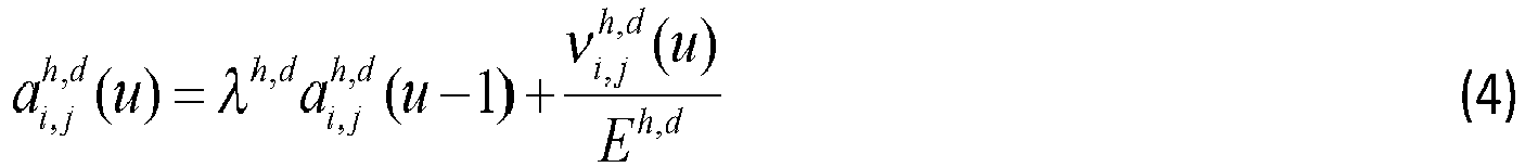
![]()
![]()
![]()
![]()
![]()
![]()
Les probabilités conditionnelles d'émission p( X t |zt ) pour les différents états de production sont calculées au moyen de la règle de Bayes, à partir des probabilités conditionnelles a posteriori p(ψj (zt )| X t ) et des probabilités a priori p(ψj (zt )), soit : 
Le module prédictif de la variable zt , prenant ses valeurs dans Sprod , est entrainé de manière supervisée dans chaque phase de calibration u selon le même principe que le modèle prédictif de chaque expert.The predictive module of the variable z t , taking its values in S prod , is trained in a supervised manner in each calibration phase u according to the same principle as the predictive model of each expert.
On rappelle que le module prédictif de l'interface REW-MSLM de l'art antérieur fournit un modèle multilinéaire optimal fopt parmi une pluralité F de modèles multilinéaires, respectivement définis par un ensemble de coefficients de prédiction ![]()
![]()
![]()
![]()
Dans le cas présent, pour chaque sous-modèle HMMh,d, l'algorithme REW-NPLS calcule une pluralité F de modèles multilinéaires définis par un ensemble de coefficients de prédiction ![]()
![]()
![]()
![]()
![]()
![]()
Les sous-modèles HMMh,d ainsi mis à jour au terme de la phase de calibration u , définis par ![]()
![]()
![]()
![]()
Il convient de rappeler que le coefficient de pondération γs,t exprime la probabilité que l'état de production s soit actif compte tenu de la séquence observée (historique du tenseur d'observation), X 1:t .It should be recalled that the weighting coefficient γ s,t expresses the probability that the production state s is active given the observed sequence (history of the observation tensor), X 1: t .
On suppose d'abord que les différents sous-modèles HMMh,d sont indépendants. L'estimation de l'état actif de chaque sous-modèle HMMh,d, peut être représenté par un vecteur ŝ h,d dont la taille est le nombre d'états du sous-modèle en question et les éléments sont représentatifs des probabilités d'activation des différents états se,h,d de ce sous-modèle, soit : ![]()
![]()
Pour chaque état de production possible, zt , on calcule la probabilité d'activation des états dans chacun des sous-modèles des couches précédentes, HMMh,d-j, j = 0,...,d au moyen de la fonction softmax : 
La probabilité conjointe de chaque état prédécesseur d'un état de production et de la séquence observée X 1:t est donnée par le processus markovien d'ordre 1 du sous-modèle HMMh,d-j à savoir : 
![]()
![]()
La probabilité conditionnelle de chaque état prédécesseur d'un état de production connaissant la séquence observée X 1:t peut être alors être calculée à partir de : 
Enfin, la probabilité γs,t = p(z t = se,h,d | X 1:t ) que l'état de production se,h,d ∈ Sprod soit actif, compte tenu de la séquence observée X 1:t , peut être obtenue comme le produit des probabilités que les états internes et l'état de production soient actifs le long du chemin conduisant à se,h,d : 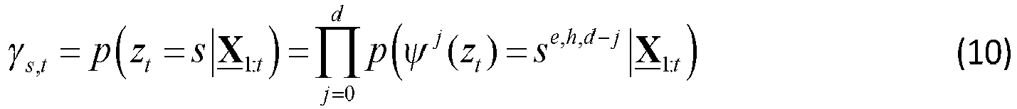
Ainsi, dans l'exemple illustré en 
A partir des coefficients de pondération ainsi calculés, le tenseur de commande peut être estimé par une combinaison des prédictions des différents experts multilinéaires : ![]()
![]()
Une seconde idée à la base de l'invention est d'utiliser dans le modèle H2M2, non plus des sous-modèles markoviens HMMh,d mais des sous-modèles semi-markoviens ou HSMM (Hidden Semi Markovian Model), notés pour cette raison HSMMh,d. Le modèle hiérarchique ainsi construit est alors noté H2SM2.A second idea underlying the invention is to use in the H2M2 model, no longer Markovian sub-models HMM h,d but semi-Markovian sub-models or HSMM (Hidden Semi Markovian Model), noted for this reason HSMM h,d . The hierarchical model thus constructed is then denoted H2SM2.
On appelle modèle semi-markovien un modèle markovien dans lequel les probabilités de transition entre états ne sont plus constantes mais dépendantes du temps. Plus précisément, la probabilité de transition, ![]()
![]()
![]()
![]()

![]()
![]()
![]()
![]()
![]()
![]()
![]()
![]()
De manière générale, certains des sous-modèles du modèle H2SM2 pourront être semi-markoviens, HSMMh,d, les autres étant simplement markoviens. De même dans un sous-modèle HSMMh,d certaines transitions entre états pourront avoir une probabilité constante dans le temps, les autres dépendant du temps comme indiqué précédemment. Si l'on note A SM (t) la matrice de transitions entre états du modèle H2SM2 la probabilité qu'un état de production du modèle soit actif à l'instant t est donnée par : ![]()
![]()
![]()
![]()
L'apprentissage du modèle H2SM2 diffère de celui du modèle H2M2 en ce que les paramètres d'évolution temporelle des transitions entre états (par exemple ![]()
![]()
![]()
![]()
Selon la variante en mode d'apprentissage supervisé, l'utilisateur reçoit des instructions de cadence pour effectuer un ou des mouvement(s) de manière répétitive (ou imaginer ces mouvements lorsque l'utilisateur est handicapé moteur), le cas échéant à différentes cadences. La cadence est fournie à l'utilisateur sous la forme de stimuli extérieurs (visuels ou sonores par exemple).According to the variant in supervised learning mode, the user receives cadence instructions to perform one or more movements in a repetitive manner (or imagine these movements when the user has motor disabilities), if necessary at different speeds. The rate is provided to the user in the form of external stimuli (visual or sound for example).
Selon la variante en mode d'apprentissage semi-supervisé, la mise à jour des paramètres du modèle ne se limite pas à la phase de calibration mais se poursuit dans la phase opérationnelle. Dans ce cas, la cadence ou de manière plus générale les informations relatives aux transitions temporelles entre états sont fournies par la sortie du décodage.According to the variant in semi-supervised learning mode, the updating of the parameters of the model is not limited to the calibration phase but continues in the operational phase. In this case, the rate or more generally the information relating to the temporal transitions between states is supplied by the output of the decoding.
La distinction entre états markoviens et états semi-markoviens peut résulter d'un choix a priori. The distinction between Markovian states and semi-Markovian states can result from an a priori choice.
Alternativement, on peut supposer que tous les états sont semi-markoviens. La durée de chaque état semi-markovien est alors enregistrée pour chacune des instances d'apprentissage. Lorsqu'une durée est supérieure à un seuil prédéterminé, l'état est considéré comme markovien. A l'inverse, si elle est inférieure à ce seuil, les paramètres d'évolution temporelle des probabilités de transition sont estimés par moyennage (instances à cadence identique) ou par régression (instances d'apprentissage à différentes cadences).Alternatively, we can assume that all states are semi-Markovian. The duration of each semi-Markov state is then recorded for each of the training instances. When a duration is greater than a predetermined threshold, the state is considered Markovian. Conversely, if it is lower than this threshold, the temporal evolution parameters of the transition probabilities are estimated by averaging (instances at the same rate) or by regression (learning instances at different rates).
La variante en mode d'apprentissage semi-supervisé opère de la même manière que dans la variante en mode supervisé, à ceci près que l'information de cadence est fournie par le décodeur lui-même. Dans un tel cas, l'utilisateur pourra être invité à effectuer différents mouvements de manière répétitive (marche par exemple) à différentes cadences, voire à penser ces mouvements lorsque l'utilisateur est handicapé moteur. Les paramètres d'évolution temporelle des probabilités de transition sont estimés et mis à jour à partir des durées respectives des états prédits par le modèle H2SM2.The variant in semi-supervised learning mode operates in the same way as in the variant in supervised mode, except that the rate information is provided by the decoder itself. In such a case, the user may be asked to perform different movements repeatedly (walking for example) at different speeds, or even to think about these movements when the user has a motor disability. The temporal evolution parameters of the transition probabilities are estimated and updated from the respective durations of the states predicted by the H2SM2 model.
Comme dans la première variante, une fois l'interface neuronale directe calibrée, les prédictions des différents experts sont combinées dans la phase opérationnelle pour estimer le tenseur de commande : ![]()
![]()
La
L'interface BCI, 400, fait intervenir, d'une part un automate à états cachés, 440, obéissant à un modèle hiérarchique markovien (H2M2) ou semi-markovien (H2SM2) et, d'autre part, une pluralité d'experts, 420, chaque estimateur (ou expert) étant associé à un état de production du modèle H2(S)M2.The BCI interface, 400, involves, on the one hand, a hidden state automaton, 440, obeying a hierarchical Markovian (H2M2) or semi-Markovian (H2SM2) model and, on the other hand, a plurality of experts , 420, each estimator (or expert) being associated with a production state of the model H2(S)M2.
Les signaux électrophysiologiques issus des capteurs 405 sont échantillonnés et rassemblés par blocs de données, chaque bloc correspondant à une fenêtre d'observation glissante définie par un instant d'observation auquel démarre la fenêtre en question. Les signaux subissent un prétraitement dans le module de prétraitement 410, comprenant notamment une analyse temps-fréquence (décomposition en ondelettes sur les fenêtres d'observation, par exemple), pour fournir un tenseur d'observation, X t , à chaque instant d'observation t.The electrophysiological signals from the
Les estimations des différents experts sont pondérées à chaque instant d'observation par des coefficients de pondération, γs,t γSM
Claims (11)
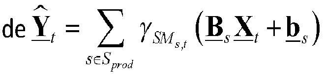
Applications Claiming Priority (1)
| Application Number | Priority Date | Filing Date | Title |
|---|---|---|---|
| FR2104905A FR3122566A1 (en) | 2021-05-10 | 2021-05-10 | DIRECT NEURONAL INTERFACE USING A HIERARCHIZED SEMI-MARKOVIAN MODEL |
Publications (1)
| Publication Number | Publication Date |
|---|---|
| EP4088659A1 true EP4088659A1 (en) | 2022-11-16 |
Family
ID=77411776
Family Applications (1)
| Application Number | Title | Priority Date | Filing Date |
|---|---|---|---|
| EP22172406.5A Pending EP4088659A1 (en) | 2021-05-10 | 2022-05-09 | Direct neural interface using a semi-markovian hierarchised model |
Country Status (2)
| Country | Link |
|---|---|
| EP (1) | EP4088659A1 (en) |
| FR (1) | FR3122566A1 (en) |
Citations (4)
| Publication number | Priority date | Publication date | Assignee | Title |
|---|---|---|---|---|
| FR3046471A1 (en) | 2016-01-06 | 2017-07-07 | Commissariat Energie Atomique | METHOD OF CALIBRATION OF A DIRECT NEURONAL INTERFACE BY PENALIZED MULTIVOIE REGRESSION |
| FR3053495A1 (en) | 2016-06-30 | 2018-01-05 | Commissariat A L'energie Atomique Et Aux Energies Alternatives | NEURONAL DIRECT INTERFACE WITH CONTINUOUS DECODING USING A MARKOVIAN MIXTURE OF EXPERTS |
| FR3061318A1 (en) | 2016-12-28 | 2018-06-29 | Commissariat A L'energie Atomique Et Aux Energies Alternatives | ITERATIVE METHOD OF CALIBRATING A DIRECT NEURONAL INTERFACE |
| EP3789852A1 (en) | 2019-09-04 | 2021-03-10 | Commissariat à l'énergie atomique et aux énergies alternatives | Method for iterative calibration of a direct neural interface using a markov mixture of experts with multivariate regression |
-
2021
- 2021-05-10 FR FR2104905A patent/FR3122566A1/en active Pending
-
2022
- 2022-05-09 EP EP22172406.5A patent/EP4088659A1/en active Pending
Patent Citations (4)
| Publication number | Priority date | Publication date | Assignee | Title |
|---|---|---|---|---|
| FR3046471A1 (en) | 2016-01-06 | 2017-07-07 | Commissariat Energie Atomique | METHOD OF CALIBRATION OF A DIRECT NEURONAL INTERFACE BY PENALIZED MULTIVOIE REGRESSION |
| FR3053495A1 (en) | 2016-06-30 | 2018-01-05 | Commissariat A L'energie Atomique Et Aux Energies Alternatives | NEURONAL DIRECT INTERFACE WITH CONTINUOUS DECODING USING A MARKOVIAN MIXTURE OF EXPERTS |
| FR3061318A1 (en) | 2016-12-28 | 2018-06-29 | Commissariat A L'energie Atomique Et Aux Energies Alternatives | ITERATIVE METHOD OF CALIBRATING A DIRECT NEURONAL INTERFACE |
| EP3789852A1 (en) | 2019-09-04 | 2021-03-10 | Commissariat à l'énergie atomique et aux énergies alternatives | Method for iterative calibration of a direct neural interface using a markov mixture of experts with multivariate regression |
Non-Patent Citations (5)
| Title |
|---|
| A. ELISEYEV ET AL.: "Recursive exponentially weighted N-way Partial Least Squares régression with recursive validation of hyper-parameters in Brain Computer Interface applications", NATURE, SCIENTIFIC REPORTS, vol. 7, 24 November 2017 (2017-11-24) |
| AMIRIBESHELI MOHSEN ET AL: "A review of smart homes in healthcare", JOURNAL OF AMBIENT INTELLIGENCE AND HUMANIZED COMPUTING, SPRINGER BERLIN HEIDELBERG, BERLIN/HEIDELBERG, vol. 6, no. 4, 14 March 2015 (2015-03-14), pages 495 - 517, XP035522418, ISSN: 1868-5137, [retrieved on 20150314], DOI: 10.1007/S12652-015-0270-2 * |
| CHUN ZHU ET AL: "Human intention recognition in Smart Assisted Living Systems using a Hierarchical Hidden Markov Model", AUTOMATION SCIENCE AND ENGINEERING, 2008. CASE 2008. IEEE INTERNATIONAL CONFERENCE ON, IEEE, PISCATAWAY, NJ, USA, 23 August 2008 (2008-08-23), pages 253 - 258, XP031321720, ISBN: 978-1-4244-2022-3 * |
| L. SRINIVASAM ET AL.: "General-purpose filter design for neural prosthetic devices", J., vol. 98, 2007, pages 2456 - 2475 |
| M. VELLISTE ET AL.: "Motor cortical correlates of arm resting in the context of a reaching task and implications for prosthetic control", THE JOURNAL OF NEUROSCIENCE, vol. 34, no. 17, 23 April 2014 (2014-04-23), pages 6011 - 6022 |
Also Published As
| Publication number | Publication date |
|---|---|
| FR3122566A1 (en) | 2022-11-11 |
Similar Documents
| Publication | Publication Date | Title |
|---|---|---|
| Betthauser et al. | Stable responsive EMG sequence prediction and adaptive reinforcement with temporal convolutional networks | |
| EP3443506B1 (en) | Artificial neuron | |
| Côté-Allard et al. | Unsupervised domain adversarial self-calibration for electromyography-based gesture recognition | |
| FR2962821A1 (en) | METHOD AND SYSTEM FOR CLASSIFYING NEURAL SIGNALS, AND METHOD FOR SELECTING ELECTRODES FOR DIRECT NEURONAL CONTROL. | |
| Puranik et al. | Heart rate estimation of PPG signals with simultaneous accelerometry using adaptive neural network filtering | |
| EP3563218B1 (en) | Iterative process for calibrating a direct neural interface | |
| FR3053495A1 (en) | NEURONAL DIRECT INTERFACE WITH CONTINUOUS DECODING USING A MARKOVIAN MIXTURE OF EXPERTS | |
| EP3789852B1 (en) | Method for iterative calibration of a direct neural interface using a markov mixture of experts with multivariate regression | |
| Karpowicz et al. | Stabilizing brain-computer interfaces through alignment of latent dynamics | |
| Wang et al. | Sequential Monte Carlo point-process estimation of kinematics from neural spiking activity for brain-machine interfaces | |
| EP3190480B1 (en) | Method for calibrating a direct neural interface by penalised multi-channel regression | |
| EP3113033B1 (en) | Stimulation therapy system, in particular of the vagus nerve, by implementing a state transition model | |
| EP4088659A1 (en) | Direct neural interface using a semi-markovian hierarchised model | |
| Costello et al. | Balancing memorization and generalization in RNNs for high performance brain-machine interfaces | |
| Seok et al. | Recognition of human motion with deep reinforcement learning | |
| Ge et al. | Sleep stages classification using neural networks with multi-channel neural data | |
| Balderas et al. | Alternative classification techniques for brain-computer interfaces for smart sensor manufacturing environments | |
| Dutta et al. | Recurrent Neural Networks and Their Application in Seizure Classification | |
| EP4024170B1 (en) | Method for self-adaptive learning of a direct neural interface using a physical detection of mental state | |
| Dantas et al. | Semi-supervised adaptive learning for decoding movement intent from electromyograms | |
| Mankar et al. | Design of adaptive filter using Jordan/Elman neural network in a typical EMG signal noise removal | |
| Sohn et al. | Feasibility of using wearable EMG armbands combined with unsupervised transfer learning for seamless myoelectric control | |
| Fountas et al. | Bayesian sense of time in biological and artificial brains | |
| Skinner et al. | Distributed classifier migration in XCS for classification of electroencephalographic signals | |
| EP4111976A1 (en) | Method for on-line calibration of a direct neural interface with determination of hyperparameters by means of reinforcement learning |
Legal Events
| Date | Code | Title | Description |
|---|---|---|---|
| PUAI | Public reference made under article 153(3) epc to a published international application that has entered the european phase |
Free format text: ORIGINAL CODE: 0009012 |
|
| STAA | Information on the status of an ep patent application or granted ep patent |
Free format text: STATUS: THE APPLICATION HAS BEEN PUBLISHED |
|
| AK | Designated contracting states |
Kind code of ref document: A1 Designated state(s): AL AT BE BG CH CY CZ DE DK EE ES FI FR GB GR HR HU IE IS IT LI LT LU LV MC MK MT NL NO PL PT RO RS SE SI SK SM TR |
|
| STAA | Information on the status of an ep patent application or granted ep patent |
Free format text: STATUS: REQUEST FOR EXAMINATION WAS MADE |
|
| 17P | Request for examination filed |
Effective date: 20230516 |
|
| RBV | Designated contracting states (corrected) |
Designated state(s): AL AT BE BG CH CY CZ DE DK EE ES FI FR GB GR HR HU IE IS IT LI LT LU LV MC MK MT NL NO PL PT RO RS SE SI SK SM TR |