EP3956696B1 - Attenuation of low-frequency noise in continously recorded wavefields - Google Patents
Attenuation of low-frequency noise in continously recorded wavefields Download PDFInfo
- Publication number
- EP3956696B1 EP3956696B1 EP20720010.6A EP20720010A EP3956696B1 EP 3956696 B1 EP3956696 B1 EP 3956696B1 EP 20720010 A EP20720010 A EP 20720010A EP 3956696 B1 EP3956696 B1 EP 3956696B1
- Authority
- EP
- European Patent Office
- Prior art keywords
- wavefield
- data
- low
- frequency noise
- source
- Prior art date
- Legal status (The legal status is an assumption and is not a legal conclusion. Google has not performed a legal analysis and makes no representation as to the accuracy of the status listed.)
- Active
Links
- 230000015572 biosynthetic process Effects 0.000 claims description 79
- 239000002245 particle Substances 0.000 claims description 79
- 230000004044 response Effects 0.000 claims description 60
- 238000000034 method Methods 0.000 claims description 55
- XLYOFNOQVPJJNP-UHFFFAOYSA-N water Substances O XLYOFNOQVPJJNP-UHFFFAOYSA-N 0.000 claims description 32
- 230000002238 attenuated effect Effects 0.000 claims description 26
- 238000013500 data storage Methods 0.000 claims description 10
- 238000002310 reflectometry Methods 0.000 claims description 3
- 238000005755 formation reaction Methods 0.000 description 74
- 230000001427 coherent effect Effects 0.000 description 30
- 230000008569 process Effects 0.000 description 22
- 238000006073 displacement reaction Methods 0.000 description 15
- 230000001133 acceleration Effects 0.000 description 14
- 238000012545 processing Methods 0.000 description 8
- 230000004913 activation Effects 0.000 description 6
- 238000011109 contamination Methods 0.000 description 6
- 238000010586 diagram Methods 0.000 description 6
- 239000000463 material Substances 0.000 description 6
- 230000000875 corresponding effect Effects 0.000 description 5
- 230000002706 hydrostatic effect Effects 0.000 description 5
- 238000012804 iterative process Methods 0.000 description 5
- 239000011159 matrix material Substances 0.000 description 5
- 230000005540 biological transmission Effects 0.000 description 4
- 230000006870 function Effects 0.000 description 4
- 230000015654 memory Effects 0.000 description 4
- 230000005012 migration Effects 0.000 description 4
- 238000013508 migration Methods 0.000 description 4
- 239000011435 rock Substances 0.000 description 4
- 239000013049 sediment Substances 0.000 description 4
- 239000004215 Carbon black (E152) Substances 0.000 description 3
- 230000003213 activating effect Effects 0.000 description 3
- 230000000694 effects Effects 0.000 description 3
- 229930195733 hydrocarbon Natural products 0.000 description 3
- 150000002430 hydrocarbons Chemical class 0.000 description 3
- 238000003384 imaging method Methods 0.000 description 3
- 238000004519 manufacturing process Methods 0.000 description 3
- 239000003208 petroleum Substances 0.000 description 3
- 238000000926 separation method Methods 0.000 description 3
- 238000001228 spectrum Methods 0.000 description 3
- 230000036962 time dependent Effects 0.000 description 3
- 230000009466 transformation Effects 0.000 description 3
- 238000004458 analytical method Methods 0.000 description 2
- 238000003491 array Methods 0.000 description 2
- 238000000605 extraction Methods 0.000 description 2
- 238000001914 filtration Methods 0.000 description 2
- 239000007788 liquid Substances 0.000 description 2
- 230000005291 magnetic effect Effects 0.000 description 2
- 238000005259 measurement Methods 0.000 description 2
- 239000000203 mixture Substances 0.000 description 2
- 230000000644 propagated effect Effects 0.000 description 2
- 230000001902 propagating effect Effects 0.000 description 2
- 238000004088 simulation Methods 0.000 description 2
- 230000007480 spreading Effects 0.000 description 2
- 238000003892 spreading Methods 0.000 description 2
- 230000001131 transforming effect Effects 0.000 description 2
- 230000000007 visual effect Effects 0.000 description 2
- 241000699670 Mus sp. Species 0.000 description 1
- 230000003044 adaptive effect Effects 0.000 description 1
- 230000002411 adverse Effects 0.000 description 1
- 230000008901 benefit Effects 0.000 description 1
- 230000015556 catabolic process Effects 0.000 description 1
- 230000008859 change Effects 0.000 description 1
- 238000012512 characterization method Methods 0.000 description 1
- 230000006835 compression Effects 0.000 description 1
- 238000007906 compression Methods 0.000 description 1
- 238000000205 computational method Methods 0.000 description 1
- 230000003750 conditioning effect Effects 0.000 description 1
- 238000010276 construction Methods 0.000 description 1
- 238000012937 correction Methods 0.000 description 1
- 230000002596 correlated effect Effects 0.000 description 1
- 238000000354 decomposition reaction Methods 0.000 description 1
- 230000007423 decrease Effects 0.000 description 1
- 238000011161 development Methods 0.000 description 1
- 230000009189 diving Effects 0.000 description 1
- 230000006872 improvement Effects 0.000 description 1
- 230000002452 interceptive effect Effects 0.000 description 1
- 230000007257 malfunction Effects 0.000 description 1
- 238000012986 modification Methods 0.000 description 1
- 230000004048 modification Effects 0.000 description 1
- 230000003287 optical effect Effects 0.000 description 1
- 230000010363 phase shift Effects 0.000 description 1
- 230000009467 reduction Effects 0.000 description 1
- 230000002829 reductive effect Effects 0.000 description 1
- 239000007787 solid Substances 0.000 description 1
- 238000003860 storage Methods 0.000 description 1
Images


Classifications
-
- G—PHYSICS
- G01—MEASURING; TESTING
- G01V—GEOPHYSICS; GRAVITATIONAL MEASUREMENTS; DETECTING MASSES OR OBJECTS; TAGS
- G01V1/00—Seismology; Seismic or acoustic prospecting or detecting
- G01V1/28—Processing seismic data, e.g. analysis, for interpretation, for correction
- G01V1/34—Displaying seismic recordings or visualisation of seismic data or attributes
- G01V1/345—Visualisation of seismic data or attributes, e.g. in 3D cubes
-
- G—PHYSICS
- G01—MEASURING; TESTING
- G01V—GEOPHYSICS; GRAVITATIONAL MEASUREMENTS; DETECTING MASSES OR OBJECTS; TAGS
- G01V1/00—Seismology; Seismic or acoustic prospecting or detecting
- G01V1/28—Processing seismic data, e.g. analysis, for interpretation, for correction
- G01V1/36—Effecting static or dynamic corrections on records, e.g. correcting spread; Correlating seismic signals; Eliminating effects of unwanted energy
- G01V1/364—Seismic filtering
-
- G—PHYSICS
- G01—MEASURING; TESTING
- G01V—GEOPHYSICS; GRAVITATIONAL MEASUREMENTS; DETECTING MASSES OR OBJECTS; TAGS
- G01V1/00—Seismology; Seismic or acoustic prospecting or detecting
- G01V1/38—Seismology; Seismic or acoustic prospecting or detecting specially adapted for water-covered areas
- G01V1/3808—Seismic data acquisition, e.g. survey design
-
- G—PHYSICS
- G01—MEASURING; TESTING
- G01V—GEOPHYSICS; GRAVITATIONAL MEASUREMENTS; DETECTING MASSES OR OBJECTS; TAGS
- G01V2210/00—Details of seismic processing or analysis
- G01V2210/10—Aspects of acoustic signal generation or detection
- G01V2210/14—Signal detection
- G01V2210/144—Signal detection with functionally associated receivers, e.g. hydrophone and geophone pairs
-
- G—PHYSICS
- G01—MEASURING; TESTING
- G01V—GEOPHYSICS; GRAVITATIONAL MEASUREMENTS; DETECTING MASSES OR OBJECTS; TAGS
- G01V2210/00—Details of seismic processing or analysis
- G01V2210/20—Trace signal pre-filtering to select, remove or transform specific events or signal components, i.e. trace-in/trace-out
- G01V2210/24—Multi-trace filtering
- G01V2210/242—F-k filtering, e.g. ground roll
-
- G—PHYSICS
- G01—MEASURING; TESTING
- G01V—GEOPHYSICS; GRAVITATIONAL MEASUREMENTS; DETECTING MASSES OR OBJECTS; TAGS
- G01V2210/00—Details of seismic processing or analysis
- G01V2210/50—Corrections or adjustments related to wave propagation
- G01V2210/56—De-ghosting; Reverberation compensation
Definitions
- Marine seismology companies invest heavily in the development of marine seismic surveying equipment and seismic data processing techniques in order to obtain accurate, high-resolution images of subterranean formations located beneath a body of water. Such images may be used, for example, to determine the structure of the subterranean formations, to discover petroleum reservoirs, and to monitor petroleum reservoirs during production.
- a typical marine seismic survey is performed with one or more survey vessels that tow one or more seismic sources and many streamers through the body of water.
- the survey vessel contains seismic acquisition equipment, such as navigation control, seismic source control, seismic receiver control, and recording equipment.
- a seismic source control controls activation of the one or more seismic sources at selected times or locations.
- a seismic source typically comprises an array of airguns that are activated to produce acoustic energy that spreads out in all directions.
- a portion of the acoustic energy travels down through the water and into a subterranean formation to propagate as sound waves within the subterranean formation.
- a portion of the acoustic energy is refracted, a portion is transmitted, and another portion is reflected into the body of water to propagate as an acoustic reflected wavefield toward the water surface.
- the streamers are elongated spaced apart cable-like structures towed behind a survey vessel in the direction the survey vessel is traveling and are typically arranged substantially parallel to one another.
- Each streamer contains many seismic receivers or sensors that measure pressure wavefield and/or particle motion wavefield properties of the reflected wavefield.
- the streamers collectively form a seismic data acquisition surface that records the pressure and/or particle motion wavefields as seismic data in the recording equipment.
- the recorded pressure and/or particle motion wavefields are processed to generate images of the subterranean formation, enabling geoscientist to identify potential hydrocarbon reservoirs that may be suitable for oil and gas extraction and to monitor hydrocarbon reservoirs under production.
- US 2017/0299743 A1 describes an interactive process that removes noise in the form of acquisition effects from continuously recorded seismic data and computes an earth response, but not extracting low-frequency noise from the earth response, computing a low-frequency noise contribution to the trace of upgoing pressure wavefield data based on the extracted low-frequency noise and the total source wavefield, and subtracting the low-frequency noise contribution to the trace of upgoing pressure wavefield data from the trace of upgoing pressure wavefield data to obtain a trace of low-frequency noise attenuated upgoing pressure wavefield data.
- US 2002/118602 A1 describes a method for attenuation of multiples in marine seismic data.
- US. 2013/0301386 describes a process that removes noise from recorded seismic data.
- Seismic imaging techniques such as wave-equation migration methods and Kirchhoff migration, generate images of a subterranean formation by numerically solving an acoustic wave equation that characterizes propagation of acoustic waves in the subterranean formation.
- Seismic imaging techniques give coordinate locations of reflections within the subterranean formation based on recorded seismic data and velocity models that represent velocities of acoustic wave propagation in the different types of liquids, rocks and sediments of the subterranean formation. The reflections occur at interfaces between layers and features of different compositions and densities, such as interfaces between layers of different kinds of rocks and sediments. The locations of reflections are displayed in an image of a seismic section of the subterranean formation.
- the image provides a visual representation of complex geophysical structures, such as layers, faults, and petroleum deposits within the subterranean formation.
- the resolution and accuracy of seismic images depend in large part on the resolution and accuracy of the velocity models.
- Accurate, high-resolution velocity models may be constructed from recorded seismic data with reliable low-frequency band information (e.g., less than about 20 Hz).
- High-resolution velocity model construction techniques such as full waveform inversion, depend on recorded seismic data that is abundant in low-frequency band information. Detailed and accurate high-resolution velocity models lead to high-resolution images and accurate characterization of complex geophysical structures.
- Seismic data recorded in a marine survey of a subterranean formation consists of signal and noise components.
- the signal component is ideally separated from the noise component and used to construct the velocity model and compute an image of the subterranean formation.
- the noise component may be any recorded energy that interferes with the desired signal component.
- Low-frequency noise contamination of the velocity model leaks into the final image, reducing image resolution and delineation of subsurface layers and reservoir boundaries.
- separation of the signal from low-frequency noise is a challenging process because of the different types of low-frequency noise.
- Examples of different types of low-frequency noise include hydrostatic pressure variation noise that ranges from about 0 - 2 Hz, streamer vibration noise that ranges from about 0 - 20 Hz, swell noise that ranges from about 1 - 15 Hz, and tugging/strumming noise from the survey vessel that ranges from about 3 - 10 Hz.
- Low-frequency streamer vibration noise is strongest near the front ends of the streamers where tension created by forcing the streamers to greater depths is greatest.
- noise attenuation techniques have been developed to attenuate low-frequency noise in recorded seismic data.
- conventional low-frequency noise attenuation techniques depend on user parameter adjustments, which is error prone, inaccurate, and time consuming.
- a method according to claim 1 for generating an image of a subterranean formation based on pressure data that were continuously recorded during a geophysical survey, the method comprising: computing upgoing pressure wavefield data at stationary-receiver locations based on continuously recorded pressure data and vertical velocity data;computing a total source wavefield based on source wavefields emitted from individual airguns of a source;attenuating low-frequency noise in the upgoing pressure wavefield based on the total source wavefield to obtain low-frequency noise attenuated upgoing pressure wavefield data at stationary-receiver locations; andgenerating an image of the subterranean formation, or data indicative thereof, based at least in part on the low-frequency noise attenuated upgoing pressure wavefield data at stationary-receiver locations, thereby reducing low frequency noise artifacts in the image, where
- the processes and systems attenuate low-frequency noise in continuously recorded seismic data, resulting in high-resolution velocity models and images of a subterranean formation with improved resolution that delineates interfaces between subsurface layers and reservoir boundaries more clearly than prior efforts to attenuate low-frequency noise.
- the low-frequency noise attenuation processes and systems may be performed on seismic data recorded with standard or large volume airguns, streamers deployed at any depth below the free surface, and without time consuming parameter adjustments associated with conventional low-frequency denoising techniques.
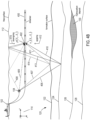
- Figures 1A-1B show a side-elevation view and a top view, respectively, of an example marine seismic data acquisition system comprising an exploration seismology survey vessel 102 and a seismic source 104.
- a seismic data acquisition system is not limited to one source as shown in Figures 1A-1B .
- the number of sources can range from as few as a single source towed by a survey vessel to as many as six or more sources towed by different survey vessels.
- the body of water can be, for example, an ocean, a sea, a lake, a river, or any portion thereof.
- the survey vessel 102 tows six streamers 106-111 located below the free surface of the body of water.
- Each streamer is attached at one end to the survey vessel 102 via a streamer data transmission cable.
- the illustrated streamers 106-111 ideally form a planar horizontal seismic data acquisition surface of the marine seismic data acquisition system with respect to the free surface 112 of the body of water.
- the streamers may be smoothly varying due to active sea currents and weather conditions.
- the streamers 106-111 are illustrated in Figures 1A and 1B to form a planar data acquisition surface, in practice, the towed streamers may undulate because of dynamic conditions of the body of water.
- a seismic data acquisition surface is not limited to a planar horizontal orientation with respect to the free surface 112.
- the seismic data acquisition surface may be angled with respect to the free surface 112 or one or more of the streamers may be towed at different depths.
- a seismic data acquisition surface is not limited to six streamers as shown in Figure 1B . In practice, the number of streamers used to form a seismic data acquisition surface can range from as few as one streamer to as many as 20 or more streamers.
- Figure 1A includes an xz-plane 114
- Figure 1B includes an xy-plane 116, of the same Cartesian coordinate system having three orthogonal, spatial coordinate axes labeled x , y and z .
- the coordinate system specifies orientations and coordinate locations within the body of water.
- the x-axis specifies the position of a point in a direction parallel to the length of the streamers or the direction of the survey vessel and is referred to as the "inline" direction.
- the y-axis specifies the position of a point in a direction perpendicular to the x-axis and substantially parallel to the free surface 112 and is referred to as the "crossline" direction.
- the z-axis also referred to as the "depth" axis, specifies the position of a point in a direction perpendicular to the xy-plane (i.e., perpendicular to the free surface 112), with the positive z-direction pointing downward away from the free surface 112.
- the streamers 106-111 are typically long cables containing power and data-transmission lines coupled to receivers (represented in the figure by shaded rectangles) such as receiver 118 that are spaced apart along the length of each streamer.
- the data transmission lines couple the receivers to seismic data acquisition equipment, computers, and data-storage devices located onboard the survey vessel 102.
- Streamer depth below the free surface 112 can be estimated at various locations along the streamers using depth-measuring devices attached to the streamers.
- the depth-measuring devices can measure hydrostatic pressure or utilize acoustic distance measurements.
- the depth-measuring devices can be integrated with depth controllers, such as paravanes or water kites that control and maintain the depth and position of the streamers as the streamers are towed through the body of water.
- depth controllers such as paravanes or water kites that control and maintain the depth and position of the streamers as the streamers are towed through the body of water.
- the depth-measuring devices are typically placed at intervals (e.g., about 300-meter intervals in some implementations) along each streamer. Note that in other implementations buoys may be attached to the streamers and used to maintain the orientation and depth of the streamers below the free surface 112.
- curve 122 the formation surface
- the subterranean formation 120 may include many subterranean layers of sediment and rock.
- Curves 124, 126, and 128 represent interfaces between subterranean layers of different compositions.
- a shaded region 130, bounded at the top by a curve 132 and at the bottom by a curve 134, represents a subterranean hydrocarbon deposit, the depth and positional coordinates of which may be determined, at least in part, by processing the seismic data collected during a marine seismic survey.
- Figure 1A shows acoustic energy expanding outward from the seismic source 104 as a pressure wavefield 136 represented by semicircles of increasing radius centered at the source 104.
- the outwardly expanding wavefronts from the source may be spherical but are shown in vertical plane cross section in Figure 1A .
- the outward and downward expanding portion of the pressure wavefield 136 is called the "source wavefield” and any portion of the pressure wavefield 136 reflected downward from the free-surface 112 is called the “source ghost wavefield.”
- the source wavefields eventually reach the formation surface 122 of the subterranean formation 120, at which point the wavefields may be partially reflected from the formation surface 122 and partially refracted downward into the subterranean formation 120, becoming elastic waves within the subterranean formation 120.
- the source wavefield primarily comprises compressional pressure waves, or P-waves, while in the subterranean formation 120, the waves include both P-waves and transverse waves, or S-waves.
- each point of the formation surface 122 and each point of the interfaces 124, 126, and 128 may be a reflector that becomes a potential secondary point source from which acoustic and elastic wave energy, respectively, may emanate upward toward the receivers 118 in response to the acoustic signals generated by the seismic source 104.
- waves of significant amplitude may be generally reflected from points on or close to the formation surface 122, such as point 138, and from points on or very close to interfaces in the subterranean formation 120, such as points 140 and 142.
- the waves comprising the reflected wavefield may be generally reflected at different times within a range of times following the source wavefield.
- a point on the formation surface 122 such as the point 144, may receive a pressure disturbance from the source wavefield more quickly than a point within the subterranean formation 120, such as points 146 and 148.
- a point on the formation surface 122 directly beneath the source 104 may receive the pressure disturbance sooner than a more distant-lying point on the formation surface 122.
- the times at which waves are reflected from various points within the subterranean formation 120 may be related to the distance, in three-dimensional space, of the points from the activated source.
- Acoustic and elastic waves may travel at different velocities within different materials as well as within the same material under different pressures. Therefore, the travel times of the source wavefield and reflected wavefield may be functions of distance from the source as well as the materials and physical characteristics of the materials through which the wavefields travel. In addition, expanding wavefronts of the wavefields may be altered as the wavefronts cross interfaces and as the velocity of sound varies in the media traversed by the wavefront.
- the superposition of waves reflected from within the subterranean formation 120 in response to the source wavefield may be a generally complicated wavefield that includes information about the shapes, sizes, and material characteristics of the subterranean formation 120, including information about the shapes, sizes, and locations of the various reflecting features within the subterranean formation 120 of interest to exploration seismologists.
- the seismic source 104 comprises multiple airguns.
- Figure 2 shows an isometric view of an example source 200.
- the source 200 comprises three sub-arrays 201-203. Each sub-array, in turn, includes six airguns in the illustrated embodiment.
- Each sub-array comprises two small volume airguns, two medium volume airguns, and two large volume airguns.
- sub-array 201 comprises two small volume airguns 204 and 205, two medium volume airguns 206 and 207, and two large volume airguns 208 and 209.
- the configuration of the three different volumes may be different for each sub-array, as it is in the illustrated embodiment.
- the spectrum of the wavefield generated by an air-gun is generally broad-band, but with peaks and notches related to a fundamental frequency called the "bubble period.”
- the volumes are selected to generate source wavefields over a broad range of frequencies.
- the large volume airguns generate source wavefields with a low fundamental frequency.
- the small volume airguns generate source wavefields with a higher fundamental frequency.
- the medium volume airguns may be selected to generate source wavefields with a fundamental frequency in between the larger and the smaller volume, and with a spectrum that complements the spectra of the wavefields generated by the other volumes.
- Each sub-array also includes pressure sensors, such as pressure sensor 210.
- Each pressure sensor is located within the near field of a corresponding airgun (e.g., about 1 meter from a corresponding airgun).
- pressure sensor 210 is located within the near field of the corresponding airgun 208.
- the sub-arrays 201-203 are suspended from corresponding floats 212-214 and connected to cables 216-218 that include electrical wires and air hoses that provide electrical activation signals and air to each airgun and transmit electrical signals generated by each pressure sensor back to the survey vessel.
- the seismic source 200 includes steering devices 220-222 that steer and control the direction of the seismic source 200 while being towed through the body of water.
- Each receiver 118 may be a multicomponent sensor including particle motion sensors and a pressure sensor.
- a pressure sensor detects variations in water pressure over time.
- the term "particle motion sensor” is a general term used to refer to a sensor that may be configured to detect particle displacement, particle velocity, or particle acceleration over time along one or more axes.
- Figure 3 shows a side-elevation view of the marine seismic data acquisition system and a magnified view 302 of the receiver 118. In this example, the magnified view 302 reveals that the receiver 118 is a multicomponent sensor comprising a pressure sensor 304 and a particle motion sensor 306.
- the pressure sensor may be, for example, a hydrophone.
- Each pressure sensor is a non-directional sensor that measures changes in a hydrostatic pressure wavefield over time to produce pressure wavefield data denoted by p x ⁇ r x ⁇ s t , where t represents time, and x ⁇ r represents the Cartesian coordinates ( x r , y r , z r ) of a receiver.
- the particle motion sensors are directional sensors that are responsive to water motion in a particular direction. In general, particle motion sensors detect particle motion (i.e., displacement, velocity, or acceleration) in a direction and may be responsive to such directional displacement of the particles, velocity of the particles, or acceleration of the particles.
- a particle motion sensor that measures particle displacement generates particle displacement data denoted by g n ⁇ x ⁇ r x ⁇ s t , where the vector n ⁇ represents the direction along which particle displacement is measured.
- a particle motion sensor that measures particle velocity i.e., particle velocity sensor
- a particle motion sensor that measures particle acceleration i.e., accelerometer
- a particle motion sensor that measures particle acceleration generates particle acceleration data denoted by a n ⁇ x ⁇ r x ⁇ s t .
- the data generated by one type of particle motion sensor may be converted to another type. For example, particle displacement data may be differentiated to obtain particle velocity wavefield data, and particle acceleration data may be integrated to obtain particle velocity data.
- particle motion data refers to particle displacement data, particle velocity wavefield data, or particle acceleration data.
- semiconductor data refers to pressure wavefield data and/or particle motion data.
- Pressure wavefield data may also be called the "pressure wavefield.”
- Particle displacement data represents a particle displacement wavefield
- particle velocity wavefield data represents a particle velocity wavefield
- particle acceleration data represents a particle acceleration wavefield.
- the particle displacement, velocity, and acceleration wavefield data are correspondingly called particle displacement, velocity, and acceleration wavefields.
- each receiver may include three particle motion sensors that measure particle motion in three orthogonal directions.
- each receiver may include a particle motion sensor that measures the wavefield in the inline direction in order to obtain the inline velocity wavefield, v x x ⁇ r x ⁇ s t , and a particle motion sensor that measures the wavefield in the crossline direction in order to obtain the crossline velocity wavefield, v y x ⁇ r x ⁇ s t .
- the receivers may be only pressure sensors, and in other implementations, the receivers may be only particle motion sensors.
- the streamers 106-111 and the survey vessel 102 may include sensing electronics and data-processing facilities that allow seismic data generated by each receiver to be correlated with the time each airgun is activated, absolute positions on the free surface 112, and absolute three-dimensional positions with respect to an arbitrary three-dimensional coordinate system.
- the pressure wavefield and particle motion wavefield may be stored at the receiver and/or may be sent along the streamers and data transmission cables to the survey vessel 102, where the data may be stored electronically, magnetically, or optically on data-storage devices located onboard the survey vessel 102 and/or transmitted onshore to data-storage devices located in a seismic data-processing facility.
- Subterranean formations located beneath a body of water may also be surveyed using ocean bottom seismic techniques.
- these techniques may be performed with ocean bottom cables ("OBCs") laid on or near the water bottom.
- OBCs are similar to towed streamers described above in that the OBCs include spaced-apart receivers, such as collocated pressure and particle motion sensors, deployed approximately every 25 to 50 meters.
- ocean bottom nodes (“OBNs") may be deployed along the formation surface. Each node may have collocated pressure and particle motion sensors.
- OBCs and OBNs may be electronically connected to an anchored recording vessel that provides power, instrument command and control of the pressure and/or vertical velocity data sent to recording equipment located on board the vessel. Traces of continuously recorded seismic data using streamers, as described above, OBCs, or OBNs may be processed as described below.
- Each pressure sensor and particle motion sensor may include an analog-to-digital converter that converts time-dependent analog signals into discrete time series data that consists of consecutively measured values called "amplitudes" separated in time by a sample rate.
- the time series data generated by a pressure or particle motion sensor is called a "trace,” which may consist of thousands of samples recorded at a typical sample rate of about 1 to 5 samples per millisecond.
- a trace includes a recording of a subterranean formation response to acoustic energy that passes from an activated source, into the subterranean formation where a portion of the acoustic energy is reflected and/or refracted, and ultimately detected by a sensor as described above.
- each trace records variations in time-dependent amplitudes that correspond to fluctuations in acoustic energy of the wavefield measured by the sensor.
- Reflected wavefields from the subterranean formation typically arrive first at the receivers located closest to the sources.
- the distance from the sources to a receiver is called the "source-receiver offset,” or simply “offset.”
- offset generally results in a longer arrival time delay.
- the traces are collected to form a “gather” that can be further processed using various seismic data processing techniques to obtain information about the structure of the subterranean formation.
- the traces may be sorted into different domains, such as a common-shot domain, common-receiver domain, common-receiver-station domain, and common-midpoint domain.
- a collection of traces sorted into the common-shot domain are called a common-shot gather and a collection of traces sorted into common-receiver domain are called a common-receiver gather.
- the portion of the acoustic signal that is reflected into the body of water from the subterranean formation and that travels directly to the receivers is called a primary reflected wavefield or simply a "primary.”
- Other portions of the acoustic energy that are reflected upward into the body of water and that reverberate between the free surface and the subterranean formation before reaching the receivers are called free-surface multiple reflected wavefields or simply "free-surface multiples.”
- Other portions of the acoustic energy that are reflected upward into the body of water directly to receivers after having reverberated within the subterranean formation are called subsurface multiple reflections or simply "subsurface multiples.”
- Figures 4A-4C show snapshots of different ways in which acoustic energy emitted from the seismic source 104 reverberates between the free surface 112 and the subterranean formation 120 before reaching the receiver 402.
- Figures 4A-4C illustrate only a few of many possible ray paths acoustic energy of an acoustic signal created by the seismic source 104 may travel before reaching the receiver 402.
- directional arrows 404-409 represent ray paths of different portions of the source wavefield generated by the seismic source 104.
- ray paths 404-407 represent portions of the source wavefield that penetrate to different interfaces of the subterranean formation 102
- ray path 408 represents a portion of the source wavefield that reaches the free surface 112.
- Ray path 409 represents the portion of the source wavefield that travels directly to the receiver 402.
- ray path 408 is extended to present a downward reflection of the source wavefield from the free surface 112 (i.e., source ghost).
- Ray paths 410 and 411 represent reflections from the interface 124 and the formation surface 122 that travel directly to the receiver 402, which are called “upgoing primary reflections" or "primaries,” as indicated by upgoing directional arrow 412.
- Ray paths 413 and 414 represent reflections from the interface 124 and the formation surface 122 followed by downward reflections from the free surface 112 before traveling directly to the receiver 402, which are called "downgoing reflections" as indicated by directional arrow 415.
- ray paths 404 and 405 are extended to represent examples of multiple reflections between interfaces within the subterranean formation 120 and the free surface 112.
- Extended ray path 404 represents a downgoing free-surface multiple.
- Extended ray path 405 represents an upgoing multiple.
- wavefields that are reflected downward from the free surface 112 before reaching the receivers are examples of “downgoing wavefields” that may also be called “ghost wavefields” or “receiver ghosts.”
- wavefields that are reflected upward from the subterranean formation 120 before reaching the receivers are examples of "upgoing wavefields.”
- Seismic data may also record acoustic energy that propagated along interfaces as head waves (not shown) before being reflected upward to the surface 122.
- Seismic data may also record acoustic energy that propagated into layers with velocity gradients that increase with depth due to compression, creating diving waves (not shown) that are gradually turned upward to the surface 122.
- Each trace records the direct source wavefield, source ghost, primaries, and various types of free surface and subsurface multiples.
- pressure wavefield p x ⁇ r , x ⁇ s , t generated at the receiver 402 records hydrostatic pressure changes due to the source wavefield, source ghost, primaries, and multiples.
- the vertical velocity wavefield v z x ⁇ r , x ⁇ s , t also generated at the receiver 402 records the particle velocity changes due to the direct source wavefield, source ghost, primaries, and multiples.
- the pressure wavefield p x ⁇ r , x ⁇ s , t and the vertical velocity wavefield v z x ⁇ r , x ⁇ s , t record both upgoing and downgoing pressure and vertical velocity wavefields, respectively, that reach the receiver 402.
- seismic data is recorded in separate shot records while a survey vessel travels along a sail line above a subterranean formation.
- a typical shot record may be created by activating airguns at the same time or, alternatively, at different times within an activation time interval, followed by recording the subterranean formation response to the source wavefield in a longer recording time interval. The process of activating the source and recording seismic data in a shot record is repeated while the survey vessel travels at a substantially constant speed along the sail line.
- Figure 5 shows an example common-shot gather of four traces of seismic data created by four adjacent receivers located along the streamer 400 shown in Figures 4A-4C obtained in a conventional marine survey.
- Vertical axis 501 represents time.
- Horizontal axis 502 represents trace numbers (i.e., channels) with trace "1" representing the seismic data generated by a receiver located closer to the seismic source 104 than trace "4" representing the seismic data generated by a receiver located farther away from the seismic source 104.
- the seismic source 104 is activated at time zero.
- the distances along the traces 504-507 from time zero to the locations of the wavelets represent travel times of the acoustic energy that is output from the seismic source 104 and eventually reaches the receivers located along the streamer 400.
- the traces 504-507 may represent variations in the amplitude of either the pressure wavefield or the particle motion wavefield measured by four adj acent receivers of the streamer 400.
- the example traces record events, such as an impulse wavefield and a reflected wavefield from a surface or interface, as wavelets located along patterned curves that correspond to the example ray paths that reach the receiver 402 in Figures 4A-4C .
- wavelets 508-511 record the source wavefield of the seismic source 104 that travels directly to the receivers as represented by dashed ray path 409 in Figure 4A .
- Wavelets 512-515 record the reflected source wavefield (i.e., source ghost) as represented by dotted ray path 408 in Figure 4B .
- Wavelets 516-519 record the primary reflected wavefield as represented by dashed-line ray path 411 in Figure 4B .
- Wavelets 520-523 record the downgoing reflected wavefield as represented by dashed-line ray path 414 in Figure 4B .
- Wavelets 524-527 record the subsurface multiple wavefield as represented by dotted-line ray path 405 in Figure 4C .
- Wavelets 528-531 record the free-surface multiple wavefield as represented by dot-dashed-line ray path 404 in Figure 4C .
- the events are identified as upgoing and downgoing wavefields as represented by the upgoing and downgoing ray paths that reach the receiver 402 in Figures 4B and 4C .
- the traces do not show various types of noise that contaminate seismic data, such as low frequency noise created by various sources.
- Continuously recorded seismic data may be obtained by activating individual airguns of a source traveling along a sail line at indiscriminate activation times and locations of the sail line, creating a continuous source wavefield with the properties of white noise. While the source travels the sail line, the continuous source wavefield interacts with the subterranean formation producing a reflected wavefield that is continuously emitted from the subterranean formation and recorded as continuously recorded seismic data by receivers.
- the terms “continuously recorded” and “recording continuously” indicate that receivers are actively recording seismic data during a period that is significantly longer than the time period in which seismic data is recorded in a shot record of a conventional marine survey. Seismic data may be continuously recorded along a sail line and yet not recorded during turning of the survey vessel while changing sail lines or during unplanned equipment downtime.
- Figure 6 shows an example of continuous recording of seismic data while a survey vessel travels along a sail line in which airguns of a seismic source are activated at indiscriminate activation times and at indiscriminate locations along the sail line.
- a survey vessel 602 tows six streamers 604 and a source 606 along a sail line 608.
- the source 606 comprises six airguns denoted by s 1 , s 2 , s 3 , s 4 , s 5 , and s 6 .
- Figure 6 includes a time axis 610 with a start time t 0 that represents the time when generation of a continuous source wavefield and continuous seismic data recording begins.
- FIG. 6 shows a gather 612 of a continuously recorded pressure or particle motion wavefield generated by pressure or particle motion sensors of one of the streamers as the survey vessel 602 travels the sail line 608.
- the gather 612 includes a receiver (i.e., channel) axis 614 and a time axis 616 that corresponds to the time axis 610 with start time t 0 and stop time T.
- Wiggle line 618 represents a trace of continuously recorded seismic data generated by pressure or particle motion sensor or sensor group as the survey vessel 602 travels the length of the sail line 608.
- any number of the traces forming a gather of continuously recorded seismic data may include breaks or blank places where no seismic data is recorded due to equipment stoppage, breakdown, or malfunction.
- a gather of continuously recorded seismic data may have any number of traces with complete, uninterrupted time samples, while other traces in the same gather may have breaks or blank places due to receiver perturbations and/or interruptions in data transmission from receivers to a data-storage device.
- Sail lines are not restricted to straight, linear lines as shown in Figure 6 .
- Sail lines may be curved, circular or any other suitable non-linear path.
- receiver locations may vary in both the x- and y -coordinate locations as a survey vessel travels a sail line.
- a survey vessel travels in a series of overlapping, near-continuously linked circular, or coiled, sail lines.
- the circular geometry of the vessel path results in acquisition of a wide range of offset seismic data across various azimuths to survey a subterranean formation in many different directions. Weather conditions and changing currents may also cause a survey vessel to deviate from a linear path.
- Processes and systems precondition the pressure and vertical velocity data by correcting the continuously recorded pressure and particle motion data for associated analogue sensor responses.
- the pressure data may be corrected for a resistor-capacitance response of the corresponding pressure sensors.
- the vertical velocity data may be corrected for responses related to a response frequency of the particle motion sensors.
- the pressure wavefield p x ⁇ r , x ⁇ s , t and vertical velocity wavefield v x x ⁇ r , x ⁇ s , t are corrected for receiver motion by associating each time sampled amplitude with the location where the time sampled amplitude was measured. Locations where the time sampled amplitudes of the continuously recorded pressure wavefield p x ⁇ r x ⁇ s t and continuously recorded vertical velocity wavefield v x x ⁇ r x ⁇ s t are measured are called stationary-receiver locations.
- P up ⁇ , k xr , k yr 1 2 ⁇ x r ⁇ y r ⁇ t p x r t , y r t , t ⁇ ⁇ k zr v z x r t , y r t , t e ⁇ i ⁇ t + k
- Each trace of a gather of seismic data at stationary-receiver locations is called a "stationary-receiver trace" that comprises seismic data recorded at a stationary-receiver location.
- the term "stationary-receiver” as used herein does not imply that a stationary receiver was used to measure the seismic data contained in a stationary-receiver trace. Because the receivers are moving during continuous seismic data recording as explained above, traces of the continuous wavefield may contain seismic data measured at about the same location.
- the transformation in Equation (2) applies a spatial phase shift to the traces of the continuous seismic data to form stationary-receiver traces that contain the seismic data as if a stationary receiver had instead been placed at the location.
- Figure 7 represents an example matrix of continuous seismic data with traces at stationary-receiver locations 700.
- Horizontal axis 701 represents stationary receiver locations in the inline direction.
- Vertical axis 702 represents time.
- Dashed line 703 represents the location of the source in front of the streamer as a function of time.
- the seismic data is confined to a diagonal strip represented by shaded region 704.
- the seismic data comprises stationary-receiver traces at stationary-receiver-locations. Unshaded portions of the matrix 700 do not contain seismic data.
- the stationary-receiver trace 705 contains the seismic data, such as pressure data, vertical velocity data, or upgoing pressure data, that would have been measured by a stationary pressure or particle motion sensor placed at the stationary-receiver location ( x str , y str ) 706.
- Angled curve 707 represents source signals emitted from the source as a function of time with different offsets relative to the receiver location.
- Dashed curves, such as dashed curve 708, represent an interface between layers of a subterranean formation with passage of time as represented by time axis 709. Bent lines illustrate portions of the source signal 707 that reflect from points on the interface and correspond to a wavelet in the stationary-receiver trace.
- bent curve 710 represents a portion of the source signal 707 that is reflected from interface 708 at a point 712 and is record in the stationary-receiver trace 705 as a wavelet 714.
- Each trace of the matrix represents the upgoing pressure wavefield at a stationary-receiver location.
- Each upgoing pressure wavefield trace of the matrix is associated with acoustic signals received from any direction and emitted at any angle from the source.
- Equation (4) the total source wavefield, S tot ( ⁇ , k xs , k ys ), is deconvolved from the upgoing pressure wavefield at stationary-receiver locations, P up ( ⁇ ).
- Figure 8 shows a relationship between an emission angle, ⁇ s , and a propagation direction 802 of an acoustic signal emitted from the source 104.
- the emission angle cannot be gleaned from a trace of upgoing pressure data at a stationary-receiver location because signals emitted from the source reach the stationary-receive location with different angles.
- an initial deconvolution is performed by spreading the received signals across the emission angles.
- the total source wavefield is deconvolved from each trace of the upgoing pressure wavefield at stationary-receiver locations, taking all possible emission angles into consideration across horizontal wavenumbers associated with the total source wavefield. Because the total source wavefield is spread across all possible source emission angles, the correct angles of emission are included in the deconvolution process.
- the total source wavefield may be iteratively deconvolved from each trace of the upgoing pressure data using the following iterative process.
- the coherent signal, E ( j ) ( ⁇ , k xs , k ys ), may be extracted from the earth response, G ⁇ ( j ) ( ⁇ , k xs , k ys ), using one or more of the following techniques.
- coherent signals located along hyperbolic trajectories within a specified velocity range are extracted. Hyperbolic reflection events of the hyperbolic trajectories in the earth response, G ( j ) ( ⁇ , k xs , k ys ), may be identified using automated semblance analysis.
- the coherent signal, E ( j ) ( ⁇ , k xs , k ys ), is extracted by filtering out signals that do not follow the identified hyperbolic reflection events.
- the coherent signal E ( j ) ( ⁇ , k xs , k ys ) corresponds to the energetic events extracted from the earth response in time and space and after plane-wave decomposition.
- the coherent signal, E ( j ) ( ⁇ , k xs , k ys ), is located within a signal cone of the earth response, G ⁇ ( j ) ( ⁇ , k xs , k ys ), and is extracted by muting portions of the earth response that are located outside the signal cone (i.e., setting to zero the incoherent signal). With each iteration, the amount of incoherent signal contamination of the earth response, G ⁇ ( i ) ( ⁇ , k xs , k ys ), decreases but may still leak into regions outside the signal cone.
- the coherent signal, E ( i ) ( ⁇ , k xs , k ys ), contains less incoherent signal contamination and is checked to determine whether the amount of incoherent signal removed is sufficient.
- the coherent signal, E ( j ) ( ⁇ , k xs , k ys ), may be transformed from the frequency-wavenumber domain to the space-time domain to obtain a coherent signal trace at a stationary-receiver location, e ( j ) ( x str ,y str , t).
- G ⁇ ⁇ k xs k ys G ⁇ final ⁇ k xs k ys + E ⁇ k xs k ys
- the earth response, G ⁇ ( ⁇ , k xs , k ys ) may be transformed from the wavenumber-frequency domain to the space-time domain to obtain an earth response trace, g ⁇ ( x str , y str , t ), at the stationary receiver location.
- Low-frequency noise is separated from the signal component of the gather of earth response traces g ⁇ (x str , y str , t ) at stationary receiver locations.
- a signal component of the earth response traces propagates with a phase or wave velocity greater than or equal to c
- the signal component lies within a signal region, or cone, defined by frequency-to-wavenumber ratios that are greater than or equal to c (i.e., ⁇ / k > c ).
- the signal cone contains signals that propagates at speeds greater than or equal to c.
- the signal cone may also contain noise that propagate at speeds greater than or equal to c.
- the signal cone may be determined by transforming earth response traces g ⁇ ( x str , y str , t ) at stationary receiver locations from the space time domain to the wavenumber-frequency domain.
- Figures 9 shows an example signal cone for an earth response trace, G ⁇ ( ⁇ , k xs , k ys ), in the wavenumber-frequency domain.
- Axis 902 represents inline wavenumbers (i.e., k x ) and axis 904 represents crossline wavenumbers (i.e., k y ).
- Axis 906 represents frequencies ( ⁇ ).
- Horizontal plane 910 is located at a frequency, ⁇ , and parallel to the inline-crossline coordinate plane.
- the horizontal plane 910 includes a light shaded circle 912 that corresponds to points located inside the signal cone 908 with the same frequency ⁇ , and dark shaded region 914 that corresponds to points located outside the signal cone 908 with the same frequency ⁇ .
- Points located inside the signal cone 908 correspond to the signal component of the earth response trace g ⁇ ( x str , y str , t ). By contrast, points located outside the signal cone 908 correspond to low-frequency noise that propagates at speeds less than the speed of sound in water c.
- Low-frequency noise may be extracted from the signal component of the gather of earth response traces g ⁇ ( x str , y str , t ) at stationary receiver locations using one of a number of different techniques.
- the low-frequency noise in the wavenumber-frequency domain, N ext ( ⁇ , k xs , k ys ) corresponds to energy in the wavenumber-frequency region located outside the signal cone for the earth response trace.
- the low-frequency noise N ext ( ⁇ , k xs , k ys ) may be obtained by muting (i.e., setting to zero) the signal component of the earth response G ⁇ ( ⁇ , k xs , k ys ) obtained in Equation (14), leaving the low-frequency noise N ext ( ⁇ , k xs , k ys ) .
- Additional techniques include, but are not limited to, detecting anomalously high amplitudes compared to background energy and extracting energy that is not coherent across the gather.
- Subtraction of the upgoing low-frequency noise at the stationary-receiver location from the upgoing pressure wavefield at the stationary-receiver location may be performed in an iterative, adaptive manner by performing the computational operations represented by Equations (8a
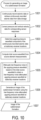
- FIG 10 is a flow diagram of a process for generating an image of a subterranean formation from continuously recorded seismic data obtained in a marine seismic survey.
- Each block represents computer implemented machine-readable instructions stored in one or more data-storage devices and executed using one or more processors of a computer system.
- the series of blocks represented in Figure 10 is not an exhaustive list of the computational operations executed to compute an image of a subterranean formation from continuously recorded seismic data. Processing may include additional computational operations or certain computational operations may be omitted or placed in a different ordering, depending on, for example, how the seismic data is collected, conditions under which the seismic data is collected, and depth of the body of water above the subterranean formation.
- block 1001 represents receiving or accessing, from data storage, continuously recorded seismic data from a survey.
- the continuously recorded seismic data may be continuously recorded pressure and vertical velocity data that were recorded using receivers configured with collocated pressure and particle motion sensors.
- the continuously recorded pressure and vertical velocity data are corrected for pressure and particle velocity sensor responses as previously described herein.
- the upgoing pressure wavefield component of the continuously recorded seismic data at stationary-receiver location is determined as described above with reference to Equation (2).
- the total source wavefield is computed from airgun measurements as described above with reference to Equation (5).
- an "attenuate low-frequency noise in the upgoing pressure wavefield to obtain low-frequency noise attenuated upgoing pressure wavefield data at stationary-receiver locations" procedure is performed.
- An example implementation of the "attenuate low-frequency noise in the upgoing pressure wavefield to obtain low-frequency noise attenuated upgoing pressure wavefield data at stationary-receiver locations" procedure is described below with reference to Figures 11 - 12 .
- an image of the subterranean formation 1006 (or data indicative thereof) is generated using the low-frequency noise attenuated upgoing pressure wavefield data at the stationary-receiver locations.
- the low-frequency noise attenuated upgoing pressure wavefield data may be used to compute a velocity model with attenuated low-frequency noise.
- the velocity model may then be used with time or depth migration applied to the low-frequency noise attenuated upgoing pressure wavefield data to obtain an image of the subterranean formation (or data indicative there, such as so-called "final migration data").
- the resulting image is not contaminated by the low-frequency noise.
- Figure 11 is a flow diagram illustrating an example implementation of the "attenuate low-frequency noise in the upgoing pressure wavefield to obtain low-frequency noise attenuated upgoing pressure wavefield data at stationary-receiver locations" procedure performed in step 1005 of Figure 10 .
- a loop beginning with block 1101 repeats the computational operations represented by blocks 1102 - 1106 for each trace of gather of the upgoing pressure wavefield at stationary-receiver locations.
- a "deconvolve the total source wavefield from the trace of upgoing pressure wavefield data to obtain an earth response to the source wavefield" procedure is performed.
- Decision block 1106 repeats blocks 1102 - 1105 for each remaining trace of the gather of the upgoing pressure wavefield at stationary-receiver locations.
- decision block 1107 the operations represented by blocks 1101 - 1106 are repeated for remaining gathers of the low-frequency noise attenuated upgoing pressure wavefield data as described above with reference to Equations (18a) and (18b).
- Figure 12 is a flow diagram illustrating an example implementation of the "deconvolve the total source wavefield from the trace of upgoing pressure wavefield data to obtain an earth response to the source wavefield" procedure performed in step 1102 of Figure 11 .
- an initial upgoing pressure wavefield is initialized using the upgoing pressure wavefield obtained in block 1003 of Figure 10 .
- a loop beginning with block 1202 iterates the computational operations represented by blocks 1203 - 1209 to obtain the earth response in block 1210.
- the earth response is computed as described above with reference to Equation (9).
- a coherent signal is extracted from the earth response computed in block 1203.
- the coherent signal may be extracted by filtering out signals that do not follow identified hyperbolic reflection events of the earth response or by muting incoherent portions of the earth response that are located outside the signal cone of the earth response.
- a contribution of coherent signals to the upgoing pressure wavefield at the stationary-receiver location is computed as described above with reference to Equation (11).
- decision block 1206 when the contribution to the coherent signal is greater than a coherent-signal threshold as described above with reference to the condition in Equation (10), control flows to block 1207.
- a coherent signal contribution to the upgoing pressure wavefield is computed as described above with reference to Equation (12).
- the trace of upgoing pressure wavefield data is updated as described above with reference to Equation (13).
- the iteration index j is incremented. If in block 1206 the contribution to the coherent signal is less than or equal to the coherent-signal threshold, then in block 1210 the earth response is computed based on the contribution of coherent signals obtained in block 1205 as described above with reference to block 1205.
- Figure 13 shows an example computer system that may be used to execute an efficient process for generating an image of subterranean formation according to methods described here, and therefore represents a geophysical-analysis data-processing system.
- the internal components of many small, mid-sized, and large computer systems as well as specialized processor-based storage systems can be described with respect to this generalized architecture, although each system may feature many additional components, subsystems, and similar, parallel systems with architectures similar to this generalized architecture.
- the computer system contains one or multiple central processing units (“CPUs”) 1302-1305, one or more electronic memories 1308 interconnected with the CPUs by a CPU/memory-subsystem bus 1310 or multiple busses, a first bridge 1312 that interconnects the CPU/memory-subsystem bus 1310 with additional busses 1314 and 1316, or other types of high-speed interconnection media, including multiple, high-speed serial interconnects.
- CPUs central processing units
- electronic memories 1308 interconnected with the CPUs by a CPU/memory-subsystem bus 1310 or multiple busses
- a first bridge 1312 that interconnects the CPU/memory-subsystem bus 1310 with additional busses 1314 and 1316, or other types of high-speed interconnection media, including multiple, high-speed serial interconnects.
- the busses or serial interconnections connect the CPUs and memory with specialized processors, such as a graphics processor 1318, and with one or more additional bridges 1320, which are interconnected with high-speed serial links or with multiple controllers 1322-1327, such as controller 1327, that provide access to various different types of computer-readable media, such as computer-readable medium 1328, electronic displays, input devices, and other such components, subcomponents, and computational resources.
- the electronic displays including visual display screen, audio speakers, and other output interfaces
- the input devices including mice, keyboards, touch screens, and other such input interfaces, together constitute input and output interfaces that allow the computer system to interact with human users.
- Computer-readable medium 1328 is a data-storage device, which may include (for example) electronic memory, optical or magnetic disk drive, a magnetic tape drive, USB drive, flash memory and any other such data-storage device or devices.
- the computer-readable medium 1328 can be used to store machine-readable instructions that encode the computational methods described above. It or similar devices can also be used to store geophysical data that results from application of the above methods to recorded seismic signals.
- the processes and systems disclosed herein may be used to manufacture a geophysical data product indicative of certain properties of a subterranean formation.
- a geophysical data product may be manufactured by using the processes and systems described herein to generate geophysical data and storing the geophysical data in a computer-readable medium 1328.
- the geophysical data may be pressure data, vertical velocity data, upgoing and downgoing wavefields, and any image of a subterranean formation computed using the processes and systems described herein.
- the geophysical data product may be produced offshore (i.e., by equipment on the survey vessel 102) or onshore (i.e., at a computing facility on land), or both.
- Figures 14A - 17E show before and after results obtained from applying the low-frequency noise attenuation processes and systems described herein to continuously recorded raw seismic data contaminated with low-frequency noise. The results shown in Figures 14A - 17E demonstrate the effectiveness of low-frequency noise attenuation processes and systems described herein.
- Figure 14A shows a gather of the raw seismic data in the space-time domain.
- the low-frequency noise appears as unevenly distributed black and white ripples that obscure reflection events 1402 (the reflection events begin to appear at about 2.5 seconds).
- Figure 14B shows a gather of the seismic data after low-frequency noise attenuation, with the reflection events readily observable and low frequency noise effects substantially reduced.
- Figure 14C shows the low-frequency noise itself, obtained by subtracting the gather in Figure 14B from the low-frequency noise contaminated gather shown in Figure 14A .
- Figure 15A shows the raw seismic data of Figure 14A transformed to the wavenumber-frequency domain. Coherent signals are located within a signal cone 1502. The low-frequency noise in the raw seismic data is exhibited by dark streaks 1504 and dark shading 1506 near the apex of the signal cone 1502.
- Figure 15B shows the raw seismic data after noise attenuation. Noise attenuation has removed the low-frequency noise exhibited by the dark streaks 1504 and dark shading 1506 in Figure 14A .
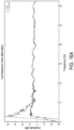
- Figure 16A shows a plot of amplitude versus frequencies for a trace of the raw seismic data before and after low-frequency noise attenuation.
- Figure 16B shows a plot of amplitudes versus base-10 log scaled frequencies for the trace of raw seismic data shown Figure 16A before and after low-frequency noise attenuation.
- dashed curves represent the amplitude variation in the raw seismic data before noise reduction and clearly show increased amplitudes over low-frequencies ranging from about 0 - 7 Hz.
- Solid curves in Figures 16A and 16B represent the seismic data after noise attenuation and clearly indicate removal of low frequency noise.
- Figures 17A - 17E show gathers of the low-frequency noise attenuated raw seismic data shown in Figure 14B for different octave bands. Figures 17A - 17E reveal how processes and systems described herein effectively attenuate low-frequency noise across the different octave bands.
Description
- This application claims the benefit of Provisional Application
62/835,018, filed April 17, 2019 - Marine seismology companies invest heavily in the development of marine seismic surveying equipment and seismic data processing techniques in order to obtain accurate, high-resolution images of subterranean formations located beneath a body of water. Such images may be used, for example, to determine the structure of the subterranean formations, to discover petroleum reservoirs, and to monitor petroleum reservoirs during production. A typical marine seismic survey is performed with one or more survey vessels that tow one or more seismic sources and many streamers through the body of water. The survey vessel contains seismic acquisition equipment, such as navigation control, seismic source control, seismic receiver control, and recording equipment. A seismic source control controls activation of the one or more seismic sources at selected times or locations. A seismic source typically comprises an array of airguns that are activated to produce acoustic energy that spreads out in all directions. A portion of the acoustic energy travels down through the water and into a subterranean formation to propagate as sound waves within the subterranean formation. At each interface between different types of liquid, rock and sediment, a portion of the acoustic energy is refracted, a portion is transmitted, and another portion is reflected into the body of water to propagate as an acoustic reflected wavefield toward the water surface. The streamers are elongated spaced apart cable-like structures towed behind a survey vessel in the direction the survey vessel is traveling and are typically arranged substantially parallel to one another. Each streamer contains many seismic receivers or sensors that measure pressure wavefield and/or particle motion wavefield properties of the reflected wavefield. The streamers collectively form a seismic data acquisition surface that records the pressure and/or particle motion wavefields as seismic data in the recording equipment. The recorded pressure and/or particle motion wavefields are processed to generate images of the subterranean formation, enabling geoscientist to identify potential hydrocarbon reservoirs that may be suitable for oil and gas extraction and to monitor hydrocarbon reservoirs under production.
-
US 2017/0299743 A1 describes an interactive process that removes noise in the form of acquisition effects from continuously recorded seismic data and computes an earth response, but not extracting low-frequency noise from the earth response, computing a low-frequency noise contribution to the trace of upgoing pressure wavefield data based on the extracted low-frequency noise and the total source wavefield, and subtracting the low-frequency noise contribution to the trace of upgoing pressure wavefield data from the trace of upgoing pressure wavefield data to obtain a trace of low-frequency noise attenuated upgoing pressure wavefield data. -
US 2002/118602 A1 describes a method for attenuation of multiples in marine seismic data.US. 2013/0301386 describes a process that removes noise from recorded seismic data. -
-
Figures 1A-1B show side-elevation and top views of an example marine seismic data acquisition system. -
Figure 2 shows an isometric view of an example source. -
Figure 3 shows a side-elevation view of an example marine seismic data acquisition system and a magnified view of a receiver. -
Figures 4A-4C show snapshots of different ways in which acoustic energy emitted from a source reverberates between a free surface and a subterranean formation before reaching a receiver. -
Figure 5 shows an example common-shot gather of four traces of seismic data created by four adjacent receivers located along a streamer. -
Figure 6 shows an example of continuous recording of seismic data. -
Figure 7 represents an example matrix of continuous seismic data with traces located at stationary-receiver locations. -
Figure 8 shows a relationship between an emission angle and propagation direction of an acoustic signal emitted from a source. -
Figure 9 shows an example signal cone for a trace of seismic data. -
Figure 10 is a flow diagram of a process for generating an image of a subterranean formation from continuously recorded seismic data obtained in a marine seismic survey. -
Figure 11 is a flow diagram illustrating an example implementation of the "attenuate low-frequency noise in the upgoing pressure wavefield to obtain low-frequency noise attenuated upgoing pressure wavefield data at stationary-receiver locations" procedure performed inFigure 10 . -
Figure 12 is a flow diagram illustrating an example implementation of the "deconvolve the total source wavefield from the trace of upgoing pressure wavefield data to obtain an earth response to the source wavefield" procedure performed inFigure 11 . -
Figure 13 shows an example computer system that may be used to execute an efficient process for generating an image of subterranean formation. -
Figures 14A - 17E show simulation results that demonstrate the effectiveness of low-frequency noise attenuation processes and systems described herein. - Seismic imaging techniques, such as wave-equation migration methods and Kirchhoff migration, generate images of a subterranean formation by numerically solving an acoustic wave equation that characterizes propagation of acoustic waves in the subterranean formation. Seismic imaging techniques give coordinate locations of reflections within the subterranean formation based on recorded seismic data and velocity models that represent velocities of acoustic wave propagation in the different types of liquids, rocks and sediments of the subterranean formation. The reflections occur at interfaces between layers and features of different compositions and densities, such as interfaces between layers of different kinds of rocks and sediments. The locations of reflections are displayed in an image of a seismic section of the subterranean formation. The image provides a visual representation of complex geophysical structures, such as layers, faults, and petroleum deposits within the subterranean formation. The resolution and accuracy of seismic images depend in large part on the resolution and accuracy of the velocity models. Accurate, high-resolution velocity models may be constructed from recorded seismic data with reliable low-frequency band information (e.g., less than about 20 Hz). High-resolution velocity model construction techniques, such as full waveform inversion, depend on recorded seismic data that is abundant in low-frequency band information. Detailed and accurate high-resolution velocity models lead to high-resolution images and accurate characterization of complex geophysical structures.
- Seismic data recorded in a marine survey of a subterranean formation consists of signal and noise components. The signal component is ideally separated from the noise component and used to construct the velocity model and compute an image of the subterranean formation. The noise component may be any recorded energy that interferes with the desired signal component. Low-frequency noise contamination of the velocity model leaks into the final image, reducing image resolution and delineation of subsurface layers and reservoir boundaries. However, separation of the signal from low-frequency noise is a challenging process because of the different types of low-frequency noise. Examples of different types of low-frequency noise include hydrostatic pressure variation noise that ranges from about 0 - 2 Hz, streamer vibration noise that ranges from about 0 - 20 Hz, swell noise that ranges from about 1 - 15 Hz, and tugging/strumming noise from the survey vessel that ranges from about 3 - 10 Hz.
- Various techniques have been developed to try and reduce the adverse effects of low-frequency noise. These include replacing certain conventional airguns in the sources with larger volume airguns to increase the low-frequency signal content in the recorded seismic data. Although large volume airguns increase the signal-to-noise ratio in recorded seismic data, which improves separation of the signal from the noise, low-frequency noise contamination persists in seismic images. Another such noise-reduction technique is to tow streamers at depths greater than the typical streamer-depth range of about 7 - 10 meters below the water surface. However, recording seismic data at depths below about 10 meters requires a substantial increase in the downward force applied the streamers, which magnifies low-frequency streamer vibration noise recorded by particle motion sensors. Low-frequency streamer vibration noise is strongest near the front ends of the streamers where tension created by forcing the streamers to greater depths is greatest. In addition, noise attenuation techniques have been developed to attenuate low-frequency noise in recorded seismic data. However, conventional low-frequency noise attenuation techniques depend on user parameter adjustments, which is error prone, inaccurate, and time consuming.
- This disclosure presents processes and systems that generate images of a subterranean formation from continuously recorded seismic data obtained in a marine seismic survey of the subterranean formation according to the claims. A method according to
claim 1 is disclosed for generating an image of a subterranean formation based on pressure data that were continuously recorded during a geophysical survey, the method comprising:
computing upgoing pressure wavefield data at stationary-receiver locations based on continuously recorded pressure data and vertical velocity data;computing a total source wavefield based on source wavefields emitted from individual airguns of a source;attenuating low-frequency noise in the upgoing pressure wavefield based on the total source wavefield to obtain low-frequency noise attenuated upgoing pressure wavefield data at stationary-receiver locations; andgenerating an image of the subterranean formation, or data indicative thereof, based at least in part on the low-frequency noise attenuated upgoing pressure wavefield data at stationary-receiver locations, thereby reducing low frequency noise artifacts in the image, wherein attenuating the low-frequency noise in the upgoing pressure wavefield to obtain the low-frequency noise attenuated upgoing pressure wavefield data at stationary-receiver locations comprises:for each trace of the upgoing pressure wavefield data at stationary-receiver locations,deconvolving the total source wavefield from the trace of upgoing pressure wavefield data to obtain an earth response to the total source wavefield;extracting low-frequency noise from the earth response computing a low-frequency noise contribution to the trace of upgoing pressure wavefield data based on the extracted low-frequency noise and the total source wavefield; andsubtracting the low-frequency noise contribution to the trace of upgoing pressure wavefield data from the trace of upgoing pressure wavefield data to obtain a trace of low-frequency noise attenuated upgoing pressure wavefield data. - The processes and systems attenuate low-frequency noise in continuously recorded seismic data, resulting in high-resolution velocity models and images of a subterranean formation with improved resolution that delineates interfaces between subsurface layers and reservoir boundaries more clearly than prior efforts to attenuate low-frequency noise. The low-frequency noise attenuation processes and systems may be performed on seismic data recorded with standard or large volume airguns, streamers deployed at any depth below the free surface, and without time consuming parameter adjustments associated with conventional low-frequency denoising techniques.
-
Figures 1A-1B show a side-elevation view and a top view, respectively, of an example marine seismic data acquisition system comprising an explorationseismology survey vessel 102 and aseismic source 104. A seismic data acquisition system is not limited to one source as shown inFigures 1A-1B . In practice, the number of sources can range from as few as a single source towed by a survey vessel to as many as six or more sources towed by different survey vessels. The body of water can be, for example, an ocean, a sea, a lake, a river, or any portion thereof. In this example, thesurvey vessel 102 tows six streamers 106-111 located below the free surface of the body of water. Each streamer is attached at one end to thesurvey vessel 102 via a streamer data transmission cable. The illustrated streamers 106-111 ideally form a planar horizontal seismic data acquisition surface of the marine seismic data acquisition system with respect to thefree surface 112 of the body of water. However, in practice, the streamers may be smoothly varying due to active sea currents and weather conditions. In other words, although the streamers 106-111 are illustrated inFigures 1A and1B to form a planar data acquisition surface, in practice, the towed streamers may undulate because of dynamic conditions of the body of water. A seismic data acquisition surface is not limited to a planar horizontal orientation with respect to thefree surface 112. The seismic data acquisition surface may be angled with respect to thefree surface 112 or one or more of the streamers may be towed at different depths. A seismic data acquisition surface is not limited to six streamers as shown inFigure 1B . In practice, the number of streamers used to form a seismic data acquisition surface can range from as few as one streamer to as many as 20 or more streamers. -
Figure 1A includes an xz-plane 114, andFigure 1B includes an xy-plane 116, of the same Cartesian coordinate system having three orthogonal, spatial coordinate axes labeled x, y and z. The coordinate system specifies orientations and coordinate locations within the body of water. The x-axis specifies the position of a point in a direction parallel to the length of the streamers or the direction of the survey vessel and is referred to as the "inline" direction. The y-axis specifies the position of a point in a direction perpendicular to the x-axis and substantially parallel to thefree surface 112 and is referred to as the "crossline" direction. The z-axis, also referred to as the "depth" axis, specifies the position of a point in a direction perpendicular to the xy-plane (i.e., perpendicular to the free surface 112), with the positive z-direction pointing downward away from thefree surface 112. - The streamers 106-111 are typically long cables containing power and data-transmission lines coupled to receivers (represented in the figure by shaded rectangles) such as
receiver 118 that are spaced apart along the length of each streamer. The data transmission lines couple the receivers to seismic data acquisition equipment, computers, and data-storage devices located onboard thesurvey vessel 102. Streamer depth below thefree surface 112 can be estimated at various locations along the streamers using depth-measuring devices attached to the streamers. For example, the depth-measuring devices can measure hydrostatic pressure or utilize acoustic distance measurements. The depth-measuring devices can be integrated with depth controllers, such as paravanes or water kites that control and maintain the depth and position of the streamers as the streamers are towed through the body of water. The depth-measuring devices are typically placed at intervals (e.g., about 300-meter intervals in some implementations) along each streamer. Note that in other implementations buoys may be attached to the streamers and used to maintain the orientation and depth of the streamers below thefree surface 112. - In
Figure 1A ,curve 122, the formation surface, represents a top surface of thesubterranean formation 120 located at the bottom of the body of water. Thesubterranean formation 120 may include many subterranean layers of sediment and rock.Curves region 130, bounded at the top by acurve 132 and at the bottom by acurve 134, represents a subterranean hydrocarbon deposit, the depth and positional coordinates of which may be determined, at least in part, by processing the seismic data collected during a marine seismic survey. As thesurvey vessel 102 moves over thesubterranean formation 120, theseismic source 104 produces acoustic energy over time that spreads out in all directions away from theseismic source 104. For the sake of simplicity,Figure 1A shows acoustic energy expanding outward from theseismic source 104 as apressure wavefield 136 represented by semicircles of increasing radius centered at thesource 104. The outwardly expanding wavefronts from the source may be spherical but are shown in vertical plane cross section inFigure 1A . The outward and downward expanding portion of thepressure wavefield 136 is called the "source wavefield" and any portion of thepressure wavefield 136 reflected downward from the free-surface 112 is called the "source ghost wavefield." The source wavefields eventually reach theformation surface 122 of thesubterranean formation 120, at which point the wavefields may be partially reflected from theformation surface 122 and partially refracted downward into thesubterranean formation 120, becoming elastic waves within thesubterranean formation 120. In the body of water, the source wavefield primarily comprises compressional pressure waves, or P-waves, while in thesubterranean formation 120, the waves include both P-waves and transverse waves, or S-waves. Within thesubterranean formation 120, at each interface between different types of materials or at discontinuities in density or in one or more of various other physical characteristics or parameters, downward propagating waves may be partially reflected and partially refracted. As a result, each point of theformation surface 122 and each point of theinterfaces receivers 118 in response to the acoustic signals generated by theseismic source 104. As shown inFigure 1A , waves of significant amplitude may be generally reflected from points on or close to theformation surface 122, such aspoint 138, and from points on or very close to interfaces in thesubterranean formation 120, such aspoints - The waves comprising the reflected wavefield may be generally reflected at different times within a range of times following the source wavefield. A point on the
formation surface 122, such as the point 144, may receive a pressure disturbance from the source wavefield more quickly than a point within thesubterranean formation 120, such as points 146 and 148. Similarly, a point on theformation surface 122 directly beneath thesource 104 may receive the pressure disturbance sooner than a more distant-lying point on theformation surface 122. Thus, the times at which waves are reflected from various points within thesubterranean formation 120 may be related to the distance, in three-dimensional space, of the points from the activated source. - Acoustic and elastic waves may travel at different velocities within different materials as well as within the same material under different pressures. Therefore, the travel times of the source wavefield and reflected wavefield may be functions of distance from the source as well as the materials and physical characteristics of the materials through which the wavefields travel. In addition, expanding wavefronts of the wavefields may be altered as the wavefronts cross interfaces and as the velocity of sound varies in the media traversed by the wavefront. The superposition of waves reflected from within the
subterranean formation 120 in response to the source wavefield may be a generally complicated wavefield that includes information about the shapes, sizes, and material characteristics of thesubterranean formation 120, including information about the shapes, sizes, and locations of the various reflecting features within thesubterranean formation 120 of interest to exploration seismologists. - The
seismic source 104 comprises multiple airguns.Figure 2 shows an isometric view of anexample source 200. Thesource 200 comprises three sub-arrays 201-203. Each sub-array, in turn, includes six airguns in the illustrated embodiment. Each sub-array comprises two small volume airguns, two medium volume airguns, and two large volume airguns. For example, sub-array 201 comprises twosmall volume airguns medium volume airguns large volume airguns pressure sensor 210. Each pressure sensor is located within the near field of a corresponding airgun (e.g., about 1 meter from a corresponding airgun). For example,pressure sensor 210 is located within the near field of thecorresponding airgun 208. The sub-arrays 201-203 are suspended from corresponding floats 212-214 and connected to cables 216-218 that include electrical wires and air hoses that provide electrical activation signals and air to each airgun and transmit electrical signals generated by each pressure sensor back to the survey vessel. In the illustrated embodiment, theseismic source 200 includes steering devices 220-222 that steer and control the direction of theseismic source 200 while being towed through the body of water.Point 224 represents the geometrical center of the array of airguns, and thus ofsource 200, with Cartesian coordinates denoted by

Figure 2 , the seismic source comprises eighteen airguns with n = 1, ...,18. - Each
receiver 118 may be a multicomponent sensor including particle motion sensors and a pressure sensor. A pressure sensor detects variations in water pressure over time. The term "particle motion sensor" is a general term used to refer to a sensor that may be configured to detect particle displacement, particle velocity, or particle acceleration over time along one or more axes.Figure 3 shows a side-elevation view of the marine seismic data acquisition system and a magnifiedview 302 of thereceiver 118. In this example, the magnifiedview 302 reveals that thereceiver 118 is a multicomponent sensor comprising apressure sensor 304 and aparticle motion sensor 306. The pressure sensor may be, for example, a hydrophone. Each pressure sensor is a non-directional sensor that measures changes in a hydrostatic pressure wavefield over time to produce pressure wavefield data denoted by


- The term "particle motion data" refers to particle displacement data, particle velocity wavefield data, or particle acceleration data. The term "seismic data" refers to pressure wavefield data and/or particle motion data. Pressure wavefield data may also be called the "pressure wavefield." Particle displacement data represents a particle displacement wavefield, particle velocity wavefield data represents a particle velocity wavefield, and particle acceleration data represents a particle acceleration wavefield. The particle displacement, velocity, and acceleration wavefield data are correspondingly called particle displacement, velocity, and acceleration wavefields.
- The particle motion sensors are typically oriented so that the particle motion is measured in the vertical direction (i.e.,


- The streamers 106-111 and the
survey vessel 102 may include sensing electronics and data-processing facilities that allow seismic data generated by each receiver to be correlated with the time each airgun is activated, absolute positions on thefree surface 112, and absolute three-dimensional positions with respect to an arbitrary three-dimensional coordinate system. The pressure wavefield and particle motion wavefield may be stored at the receiver and/or may be sent along the streamers and data transmission cables to thesurvey vessel 102, where the data may be stored electronically, magnetically, or optically on data-storage devices located onboard thesurvey vessel 102 and/or transmitted onshore to data-storage devices located in a seismic data-processing facility. - Subterranean formations located beneath a body of water may also be surveyed using ocean bottom seismic techniques. In one implementation, these techniques may be performed with ocean bottom cables ("OBCs") laid on or near the water bottom. The OBCs are similar to towed streamers described above in that the OBCs include spaced-apart receivers, such as collocated pressure and particle motion sensors, deployed approximately every 25 to 50 meters. In another implementation, ocean bottom nodes ("OBNs") may be deployed along the formation surface. Each node may have collocated pressure and particle motion sensors. The OBCs and OBNs may be electronically connected to an anchored recording vessel that provides power, instrument command and control of the pressure and/or vertical velocity data sent to recording equipment located on board the vessel. Traces of continuously recorded seismic data using streamers, as described above, OBCs, or OBNs may be processed as described below.
- Each pressure sensor and particle motion sensor may include an analog-to-digital converter that converts time-dependent analog signals into discrete time series data that consists of consecutively measured values called "amplitudes" separated in time by a sample rate. The time series data generated by a pressure or particle motion sensor is called a "trace," which may consist of thousands of samples recorded at a typical sample rate of about 1 to 5 samples per millisecond. A trace includes a recording of a subterranean formation response to acoustic energy that passes from an activated source, into the subterranean formation where a portion of the acoustic energy is reflected and/or refracted, and ultimately detected by a sensor as described above. Each trace records variations in time-dependent amplitudes that correspond to fluctuations in acoustic energy of the wavefield measured by the sensor. In general, each trace is an ordered set of discrete spatial and time-dependent pressure or motion sensor amplitudes denoted by:

- tr represents a trace of pressure, particle displacement, particle velocity, or particle acceleration data;
- A represents an amplitude of pressure, particle displacement, particle velocity, or particle acceleration data at the time sample;
- tl is the l-th sample time; and
- L is the number of time samples in the trace.
- Reflected wavefields from the subterranean formation typically arrive first at the receivers located closest to the sources. The distance from the sources to a receiver is called the "source-receiver offset," or simply "offset." A larger offset generally results in a longer arrival time delay. The traces are collected to form a "gather" that can be further processed using various seismic data processing techniques to obtain information about the structure of the subterranean formation. The traces may be sorted into different domains, such as a common-shot domain, common-receiver domain, common-receiver-station domain, and common-midpoint domain. For example, a collection of traces sorted into the common-shot domain are called a common-shot gather and a collection of traces sorted into common-receiver domain are called a common-receiver gather. The portion of the acoustic signal that is reflected into the body of water from the subterranean formation and that travels directly to the receivers is called a primary reflected wavefield or simply a "primary." Other portions of the acoustic energy that are reflected upward into the body of water and that reverberate between the free surface and the subterranean formation before reaching the receivers are called free-surface multiple reflected wavefields or simply "free-surface multiples." Other portions of the acoustic energy that are reflected upward into the body of water directly to receivers after having reverberated within the subterranean formation are called subsurface multiple reflections or simply "subsurface multiples."
-
Figures 4A-4C show snapshots of different ways in which acoustic energy emitted from theseismic source 104 reverberates between thefree surface 112 and thesubterranean formation 120 before reaching thereceiver 402. For the sake of simplicity,Figures 4A-4C illustrate only a few of many possible ray paths acoustic energy of an acoustic signal created by theseismic source 104 may travel before reaching thereceiver 402. InFigure 4A , directional arrows 404-409 represent ray paths of different portions of the source wavefield generated by theseismic source 104. For example, ray paths 404-407 represent portions of the source wavefield that penetrate to different interfaces of thesubterranean formation 102, andray path 408 represents a portion of the source wavefield that reaches thefree surface 112.Ray path 409 represents the portion of the source wavefield that travels directly to thereceiver 402. InFigure 4B ,ray path 408 is extended to present a downward reflection of the source wavefield from the free surface 112 (i.e., source ghost).Ray paths interface 124 and theformation surface 122 that travel directly to thereceiver 402, which are called "upgoing primary reflections" or "primaries," as indicated by upgoingdirectional arrow 412.Ray paths interface 124 and theformation surface 122 followed by downward reflections from thefree surface 112 before traveling directly to thereceiver 402, which are called "downgoing reflections" as indicated bydirectional arrow 415. InFigure 4C ,ray paths subterranean formation 120 and thefree surface 112.Extended ray path 404 represents a downgoing free-surface multiple.Extended ray path 405 represents an upgoing multiple. InFigures 4B-4C , wavefields that are reflected downward from thefree surface 112 before reaching the receivers, as represented byray paths Figures 4B-4C , wavefields that are reflected upward from thesubterranean formation 120 before reaching the receivers, as represented byray paths surface 122. Seismic data may also record acoustic energy that propagated into layers with velocity gradients that increase with depth due to compression, creating diving waves (not shown) that are gradually turned upward to thesurface 122. - Each trace records the direct source wavefield, source ghost, primaries, and various types of free surface and subsurface multiples. For example, pressure wavefield

receiver 402 records hydrostatic pressure changes due to the source wavefield, source ghost, primaries, and multiples. The vertical velocity wavefield
receiver 402 records the particle velocity changes due to the direct source wavefield, source ghost, primaries, and multiples. The pressure wavefield

receiver 402. - In a conventional marine survey, seismic data is recorded in separate shot records while a survey vessel travels along a sail line above a subterranean formation. A typical shot record may be created by activating airguns at the same time or, alternatively, at different times within an activation time interval, followed by recording the subterranean formation response to the source wavefield in a longer recording time interval. The process of activating the source and recording seismic data in a shot record is repeated while the survey vessel travels at a substantially constant speed along the sail line.
-
Figure 5 shows an example common-shot gather of four traces of seismic data created by four adjacent receivers located along thestreamer 400 shown inFigures 4A-4C obtained in a conventional marine survey.Vertical axis 501 represents time.Horizontal axis 502 represents trace numbers (i.e., channels) with trace "1" representing the seismic data generated by a receiver located closer to theseismic source 104 than trace "4" representing the seismic data generated by a receiver located farther away from theseismic source 104. Theseismic source 104 is activated at time zero. The distances along the traces 504-507 from time zero to the locations of the wavelets represent travel times of the acoustic energy that is output from theseismic source 104 and eventually reaches the receivers located along thestreamer 400. The traces 504-507 may represent variations in the amplitude of either the pressure wavefield or the particle motion wavefield measured by four adj acent receivers of thestreamer 400. The example traces record events, such as an impulse wavefield and a reflected wavefield from a surface or interface, as wavelets located along patterned curves that correspond to the example ray paths that reach thereceiver 402 inFigures 4A-4C . For example, wavelets 508-511 record the source wavefield of theseismic source 104 that travels directly to the receivers as represented by dashedray path 409 inFigure 4A . Wavelets 512-515 record the reflected source wavefield (i.e., source ghost) as represented by dottedray path 408 inFigure 4B . Wavelets 516-519 record the primary reflected wavefield as represented by dashed-line ray path 411 inFigure 4B . Wavelets 520-523 record the downgoing reflected wavefield as represented by dashed-line ray path 414 inFigure 4B . Wavelets 524-527 record the subsurface multiple wavefield as represented by dotted-line ray path 405 inFigure 4C . Wavelets 528-531 record the free-surface multiple wavefield as represented by dot-dashed-line ray path 404 inFigure 4C . InFigure 5 , the events are identified as upgoing and downgoing wavefields as represented by the upgoing and downgoing ray paths that reach thereceiver 402 inFigures 4B and4C . For the sake of convenience, the traces do not show various types of noise that contaminate seismic data, such as low frequency noise created by various sources. - Processes and systems described herein attenuate low-frequency noise in continuously recorded seismic data obtained in a marine survey of a subterranean formation. Continuously recorded seismic data may be obtained by activating individual airguns of a source traveling along a sail line at indiscriminate activation times and locations of the sail line, creating a continuous source wavefield with the properties of white noise. While the source travels the sail line, the continuous source wavefield interacts with the subterranean formation producing a reflected wavefield that is continuously emitted from the subterranean formation and recorded as continuously recorded seismic data by receivers.
- In the following discussion, the terms "continuously recorded" and "recording continuously" indicate that receivers are actively recording seismic data during a period that is significantly longer than the time period in which seismic data is recorded in a shot record of a conventional marine survey. Seismic data may be continuously recorded along a sail line and yet not recorded during turning of the survey vessel while changing sail lines or during unplanned equipment downtime.
-
Figure 6 shows an example of continuous recording of seismic data while a survey vessel travels along a sail line in which airguns of a seismic source are activated at indiscriminate activation times and at indiscriminate locations along the sail line. InFigure 6 , asurvey vessel 602 tows sixstreamers 604 and asource 606 along asail line 608. In this example, thesource 606 comprises six airguns denoted by s 1, s 2, s 3, s 4, s 5, and s 6.Figure 6 includes atime axis 610 with a start time t 0 that represents the time when generation of a continuous source wavefield and continuous seismic data recording begins. The point in time when recording along thesail line 608 stops is represented by stop time T. Closed circles labeled s 1, s 2, s 3, s 4, s 5, and s 6 represent randomized or pseudo-randomized activation times when the airguns are activated between the start time t 0 and the stop time T.Figure 6 also shows a gather 612 of a continuously recorded pressure or particle motion wavefield generated by pressure or particle motion sensors of one of the streamers as thesurvey vessel 602 travels thesail line 608. The gather 612 includes a receiver (i.e., channel)axis 614 and atime axis 616 that corresponds to thetime axis 610 with start time t 0 and stop time T. Closed circles located along thetime axis 616 correspond to times when the airguns are activated along thetime axis 610.Wiggle line 618 represents a trace of continuously recorded seismic data generated by pressure or particle motion sensor or sensor group as thesurvey vessel 602 travels the length of thesail line 608. - In practice, any number of the traces forming a gather of continuously recorded seismic data may include breaks or blank places where no seismic data is recorded due to equipment stoppage, breakdown, or malfunction. For example, a gather of continuously recorded seismic data may have any number of traces with complete, uninterrupted time samples, while other traces in the same gather may have breaks or blank places due to receiver perturbations and/or interruptions in data transmission from receivers to a data-storage device.
- Sail lines are not restricted to straight, linear lines as shown in
Figure 6 . Sail lines may be curved, circular or any other suitable non-linear path. In other words, receiver locations may vary in both the x- and y-coordinate locations as a survey vessel travels a sail line. For example, in coil shooting surveys, a survey vessel travels in a series of overlapping, near-continuously linked circular, or coiled, sail lines. The circular geometry of the vessel path results in acquisition of a wide range of offset seismic data across various azimuths to survey a subterranean formation in many different directions. Weather conditions and changing currents may also cause a survey vessel to deviate from a linear path. - Processes and systems precondition the pressure and vertical velocity data by correcting the continuously recorded pressure and particle motion data for associated analogue sensor responses. For example, the pressure data may be corrected for a resistor-capacitance response of the corresponding pressure sensors. The vertical velocity data may be corrected for responses related to a response frequency of the particle motion sensors.
- Following pre-conditioning, the pressure wavefield


-

- kxr is a horizontal wavenumber in the inline direction at a receiver;
- kyr is a horizontal wavenumber in the crossline direction at a receiver;
- ω is angular frequency;
- ρ is the density of the body of water;
-

- c is the speed of sound in water;
- p(xr (t), yr (t), t) is the continuously recorded pressure wavefield; and
- vz (xr (t), yr (t), t) is the continuously recorded vertical velocity.
- Each trace of a gather of seismic data at stationary-receiver locations is called a "stationary-receiver trace" that comprises seismic data recorded at a stationary-receiver location. The term "stationary-receiver" as used herein does not imply that a stationary receiver was used to measure the seismic data contained in a stationary-receiver trace. Because the receivers are moving during continuous seismic data recording as explained above, traces of the continuous wavefield may contain seismic data measured at about the same location. The transformation in Equation (2) applies a spatial phase shift to the traces of the continuous seismic data to form stationary-receiver traces that contain the seismic data as if a stationary receiver had instead been placed at the location. When OBCs are used to record seismic data on the surface of the subterranean formation, correction for receiver motion described above may be omitted.
-
Figure 7 represents an example matrix of continuous seismic data with traces at stationary-receiver locations 700.Horizontal axis 701 represents stationary receiver locations in the inline direction.Vertical axis 702 represents time. Dashedline 703 represents the location of the source in front of the streamer as a function of time. The seismic data is confined to a diagonal strip represented by shadedregion 704. The seismic data comprises stationary-receiver traces at stationary-receiver-locations. Unshaded portions of thematrix 700 do not contain seismic data. The stationary-receiver trace 705 contains the seismic data, such as pressure data, vertical velocity data, or upgoing pressure data, that would have been measured by a stationary pressure or particle motion sensor placed at the stationary-receiver location (xstr , ystr ) 706.Angled curve 707 represents source signals emitted from the source as a function of time with different offsets relative to the receiver location. Dashed curves, such as dashedcurve 708, represent an interface between layers of a subterranean formation with passage of time as represented bytime axis 709. Bent lines illustrate portions of the source signal 707 that reflect from points on the interface and correspond to a wavelet in the stationary-receiver trace. For example,bent curve 710 represents a portion of the source signal 707 that is reflected frominterface 708 at apoint 712 and is record in the stationary-receiver trace 705 as awavelet 714. - Each trace of the matrix represents the upgoing pressure wavefield at a stationary-receiver location. Each upgoing pressure wavefield trace of the matrix is associated with acoustic signals received from any direction and emitted at any angle from the source. In the space-frequency domain, the upgoing pressure wavefield at each stationary-receiver location is given by:

- kxs is the source wavenumber in the inline direction;
- kys is the source wavenumber in the crossline direction;
- Stot (ω, kxs, kys ) is the total source wavefield emitted from the source; and
- G(ω, kxs, kys ) is the earth response to the total source wavefield.
- The total source wavefield emitted from the source, used in Equation (4), may be represented by

- [e -ik
zs zsn - Reikzs zsn ] is a ghost function that re-datums the source wavefield to the free surface; -

- R is the reflectivity of the free surface; and
- sn (t, xsn , ysn ) is the signal emitted by a airgun of the source at location (xsn, ysn ) (See
Figure 2 ). - In order to extract the earth response, G(ω, kxs, kys ), from Equation (4), the total source wavefield, Stot (ω, kxs, kys ), is deconvolved from the upgoing pressure wavefield at stationary-receiver locations, Pup (ω). The emission angle of an acoustic signal emitted from the source is related to the frequency of the emitted signal and the vertical wavenumber of the source by

θs is the emission angle of an acoustic signal from the source.
Figure 8 shows a relationship between an emission angle, θs , and apropagation direction 802 of an acoustic signal emitted from thesource 104. The emission angle cannot be gleaned from a trace of upgoing pressure data at a stationary-receiver location because signals emitted from the source reach the stationary-receive location with different angles. In order to determine the emission angles that are in a trace of upgoing pressure data at a stationary-receiver location, an initial deconvolution is performed by spreading the received signals across the emission angles. This initial source deconvolution can be expressed as
- Pup (ω) is the upgoing pressure data in Equation (4);
- w(ω) is a user-defined output wavelet; and
- G̃(ω, kxs, kys ) is the estimated earth response of a common-receiver gather.
- The total source wavefield is deconvolved from each trace of the upgoing pressure wavefield at stationary-receiver locations, taking all possible emission angles into consideration across horizontal wavenumbers associated with the total source wavefield. Because the total source wavefield is spread across all possible source emission angles, the correct angles of emission are included in the deconvolution process. The total source wavefield may be iteratively deconvolved from each trace of the upgoing pressure data using the following iterative process.
- Let j denote an iteration index such that a superscript "(j)" in the following equations denotes
iterative steps 

- The earth response may be iteratively computed for j = 1, 2, 3, ... using Equation (7) as follows:

- After the earth response, G̃ (j)(ω, kxs, kys ), is calculated for each iteration, the coherent signal, E (j)(ω, kxs, kys ), may be extracted from the earth response, G̃ (j)(ω, kxs, kys ), using one or more of the following techniques. In one implementation, coherent signals located along hyperbolic trajectories within a specified velocity range are extracted. Hyperbolic reflection events of the hyperbolic trajectories in the earth response, G (j)(ω, kxs, kys ), may be identified using automated semblance analysis. The coherent signal, E (j)(ω, kxs, kys ), is extracted by filtering out signals that do not follow the identified hyperbolic reflection events. In another implementation, the coherent signal E (j)(ω, kxs, kys ) corresponds to the energetic events extracted from the earth response in time and space and after plane-wave decomposition. The coherent signal, E (j)(ω, kxs, kys ), is located within a signal cone of the earth response, G̃ (j)(ω, kxs, kys ), and is extracted by muting portions of the earth response that are located outside the signal cone (i.e., setting to zero the incoherent signal). With each iteration, the amount of incoherent signal contamination of the earth response, G̃ (i)(ω, kxs, kys ), decreases but may still leak into regions outside the signal cone. Muting portions of the earth response that are located outside the signal cone gives the coherent signal, E (j)(ω, kxs, kys ), with less incoherent signal contamination than the coherent signal, E (j-1)(ω, kxs, kys ), that was obtained in the previous iteration. The extracted coherent signal, E (j)(ω, kxs, kys ), for each iteration contains angle information.
- After each iterative extraction of the coherent signal E (j)(ω, kxs, kys ) from the earth response G̃ (j)(ω, kxs, kys ), the coherent signal, E (i)(ω, kxs, kys ), contains less incoherent signal contamination and is checked to determine whether the amount of incoherent signal removed is sufficient. The coherent signal, E (j)(ω, kxs, kys ), may be transformed from the frequency-wavenumber domain to the space-time domain to obtain a coherent signal trace at a stationary-receiver location, e (j)(xstr,ystr, t). The iterative process stops when the following condition is satisfied

- e (j)(xstr, ystr, tl ) is an amplitude at time sample tl of the coherent signal trace e (j)(xstr, ystr , t); and
- Th is a user-defined coherent-signal threshold.
- When the iterative process stops because the condition in Equation (10) is satisfied, the coherent signals, E (j)(ω, kxs, kys ), can no longer be extracted from the earth response, G̃ (j)(ω, kxs, kys ). Let G̃ (final)(ω, kxs, kys ) represent a final earth response obtained from Equation (9) with extracted coherent signals E (j)(ω, kxs, kys ) that do not satisfy the condition in Equation (10). The contribution of the coherent signals, E(ω, kxs, kys ), are added to the final earth response to give:

- Low-frequency noise is separated from the signal component of the gather of earth response traces g̃(xstr, ystr, t) at stationary receiver locations. The frequency ω of a sound wave, wavenumber k of the sound wave, and speed c of the sound wave propagating in water are related by ω = kc. Because a signal component of the earth response traces propagates with a phase or wave velocity greater than or equal to c, the signal component lies within a signal region, or cone, defined by frequency-to-wavenumber ratios that are greater than or equal to c (i.e., ω/k > c). The signal cone contains signals that propagates at speeds greater than or equal to c. The signal cone may also contain noise that propagate at speeds greater than or equal to c. The signal cone may be determined by transforming earth response traces g̃(xstr , ystr, t) at stationary receiver locations from the space time domain to the wavenumber-frequency domain.
-
Figures 9 shows an example signal cone for an earth response trace, G̃(ω, kxs, kys ), in the wavenumber-frequency domain.Axis 902 represents inline wavenumbers (i.e., kx ) andaxis 904 represents crossline wavenumbers (i.e., ky ).Axis 906 represents frequencies (ω). Asignal cone 908 is a region in the wavenumber-frequency domain with a cone boundary for frequencies and horizontal wavenumbers given by:
Horizontal plane 910 is located at a frequency, ω, and parallel to the inline-crossline coordinate plane. Thehorizontal plane 910 includes a lightshaded circle 912 that corresponds to points located inside thesignal cone 908 with the same frequency ω, and darkshaded region 914 that corresponds to points located outside thesignal cone 908 with the same frequency ω. Points located in thehorizontal plane 910 and outside the signal cone in thedark shade region 914, such as point (ω, k x1 , k y1) 916, have speeds that are less than the speed of sound in water c. Points located in thehorizontal plane 910 and inside thelight shade circle 912, such as point (ω, k x2, k y2) 918, have speeds that are greater than the speed of sound in water c. Points located inside thesignal cone 908 correspond to the signal component of the earth response trace g̃(xstr , ystr , t). By contrast, points located outside thesignal cone 908 correspond to low-frequency noise that propagates at speeds less than the speed of sound in water c. - Low-frequency noise, denoted by next (xstr , ystr, t), may be extracted from the signal component of the gather of earth response traces g̃(xstr , ystr , t) at stationary receiver locations using one of a number of different techniques. For example, the low-frequency noise in the wavenumber-frequency domain, Next (ω, kxs, kys ), corresponds to energy in the wavenumber-frequency region located outside the signal cone for the earth response trace. The low-frequency noise Next (ω, kxs, kys ) may be obtained by muting (i.e., setting to zero) the signal component of the earth response G̃(ω, kxs, kys ) obtained in Equation (14), leaving the low-frequency noise Next (ω, kxs, kys ). Additional techniques include, but are not limited to, detecting anomalously high amplitudes compared to background energy and extracting energy that is not coherent across the gather. The low-frequency noise contribution to the upgoing pressure wavefield at the stationary-receiver location is given by


-
Figure 10 is a flow diagram of a process for generating an image of a subterranean formation from continuously recorded seismic data obtained in a marine seismic survey. Each block represents computer implemented machine-readable instructions stored in one or more data-storage devices and executed using one or more processors of a computer system. It should be noted that the series of blocks represented inFigure 10 is not an exhaustive list of the computational operations executed to compute an image of a subterranean formation from continuously recorded seismic data. Processing may include additional computational operations or certain computational operations may be omitted or placed in a different ordering, depending on, for example, how the seismic data is collected, conditions under which the seismic data is collected, and depth of the body of water above the subterranean formation. - In
Figure 10 ,block 1001 represents receiving or accessing, from data storage, continuously recorded seismic data from a survey. For example, the continuously recorded seismic data may be continuously recorded pressure and vertical velocity data that were recorded using receivers configured with collocated pressure and particle motion sensors. Inblock 1002, the continuously recorded pressure and vertical velocity data are corrected for pressure and particle velocity sensor responses as previously described herein. Inblock 1003, the upgoing pressure wavefield component of the continuously recorded seismic data at stationary-receiver location is determined as described above with reference to Equation (2). Inblock 1004, the total source wavefield is computed from airgun measurements as described above with reference to Equation (5). Inblock 1005, an "attenuate low-frequency noise in the upgoing pressure wavefield to obtain low-frequency noise attenuated upgoing pressure wavefield data at stationary-receiver locations" procedure is performed. An example implementation of the "attenuate low-frequency noise in the upgoing pressure wavefield to obtain low-frequency noise attenuated upgoing pressure wavefield data at stationary-receiver locations" procedure is described below with reference toFigures 11 - 12 . Inblock 1006, an image of the subterranean formation 1006 (or data indicative thereof) is generated using the low-frequency noise attenuated upgoing pressure wavefield data at the stationary-receiver locations. The low-frequency noise attenuated upgoing pressure wavefield data may be used to compute a velocity model with attenuated low-frequency noise. The velocity model may then be used with time or depth migration applied to the low-frequency noise attenuated upgoing pressure wavefield data to obtain an image of the subterranean formation (or data indicative there, such as so-called "final migration data"). The resulting image is not contaminated by the low-frequency noise. -
Figure 11 is a flow diagram illustrating an example implementation of the "attenuate low-frequency noise in the upgoing pressure wavefield to obtain low-frequency noise attenuated upgoing pressure wavefield data at stationary-receiver locations" procedure performed instep 1005 ofFigure 10 . A loop beginning withblock 1101 repeats the computational operations represented by blocks 1102 - 1106 for each trace of gather of the upgoing pressure wavefield at stationary-receiver locations. Inblock 1102, a "deconvolve the total source wavefield from the trace of upgoing pressure wavefield data to obtain an earth response to the source wavefield" procedure is performed. An example implementation of the "deconvolve the total source wavefield from the trace of upgoing pressure wavefield data to obtain an earth response to the source wavefield" procedure is described below with reference toFigure 12 . Inblock 1103, low-frequency noise is extracted from the earth response as described above with reference toFigure 9 . Inblock 1104, a low-frequency noise contribution to the upgoing pressure wavefield is computed based on the extracted low-frequency noise and the total source wavefield as described above with reference to Equation (16). Inblock 1105, the low-frequency noise contribution to the upgoing pressure wavefield is subtracted from the trace of upgoing pressure wavefield data to obtain a trace of noise attenuated upgoing pressure wavefield data as described above with reference to Equation (17).Decision block 1106 repeats blocks 1102 - 1105 for each remaining trace of the gather of the upgoing pressure wavefield at stationary-receiver locations. Indecision block 1107, the operations represented by blocks 1101 - 1106 are repeated for remaining gathers of the low-frequency noise attenuated upgoing pressure wavefield data as described above with reference to Equations (18a) and (18b). -
Figure 12 is a flow diagram illustrating an example implementation of the "deconvolve the total source wavefield from the trace of upgoing pressure wavefield data to obtain an earth response to the source wavefield" procedure performed instep 1102 ofFigure 11 . Inblock 1201, an initial upgoing pressure wavefield is initialized using the upgoing pressure wavefield obtained inblock 1003 ofFigure 10 . A loop beginning withblock 1202 iterates the computational operations represented by blocks 1203 - 1209 to obtain the earth response inblock 1210. Inblock 1203, the earth response is computed as described above with reference to Equation (9). Inblock 1204, a coherent signal is extracted from the earth response computed inblock 1203. For example, the coherent signal may be extracted by filtering out signals that do not follow identified hyperbolic reflection events of the earth response or by muting incoherent portions of the earth response that are located outside the signal cone of the earth response. Inblock 1205, a contribution of coherent signals to the upgoing pressure wavefield at the stationary-receiver location is computed as described above with reference to Equation (11). Indecision block 1206, when the contribution to the coherent signal is greater than a coherent-signal threshold as described above with reference to the condition in Equation (10), control flows to block 1207. Inblock 1207, a coherent signal contribution to the upgoing pressure wavefield is computed as described above with reference to Equation (12). Inblock 1208, the trace of upgoing pressure wavefield data is updated as described above with reference to Equation (13). Inblock 1209, the iteration index j is incremented. If inblock 1206 the contribution to the coherent signal is less than or equal to the coherent-signal threshold, then inblock 1210 the earth response is computed based on the contribution of coherent signals obtained inblock 1205 as described above with reference to block 1205. -
Figure 13 shows an example computer system that may be used to execute an efficient process for generating an image of subterranean formation according to methods described here, and therefore represents a geophysical-analysis data-processing system. The internal components of many small, mid-sized, and large computer systems as well as specialized processor-based storage systems can be described with respect to this generalized architecture, although each system may feature many additional components, subsystems, and similar, parallel systems with architectures similar to this generalized architecture. The computer system contains one or multiple central processing units ("CPUs") 1302-1305, one or moreelectronic memories 1308 interconnected with the CPUs by a CPU/memory-subsystem bus 1310 or multiple busses, afirst bridge 1312 that interconnects the CPU/memory-subsystem bus 1310 withadditional busses graphics processor 1318, and with one or moreadditional bridges 1320, which are interconnected with high-speed serial links or with multiple controllers 1322-1327, such ascontroller 1327, that provide access to various different types of computer-readable media, such as computer-readable medium 1328, electronic displays, input devices, and other such components, subcomponents, and computational resources. The electronic displays, including visual display screen, audio speakers, and other output interfaces, and the input devices, including mice, keyboards, touch screens, and other such input interfaces, together constitute input and output interfaces that allow the computer system to interact with human users. Computer-readable medium 1328 is a data-storage device, which may include (for example) electronic memory, optical or magnetic disk drive, a magnetic tape drive, USB drive, flash memory and any other such data-storage device or devices. The computer-readable medium 1328 can be used to store machine-readable instructions that encode the computational methods described above. It or similar devices can also be used to store geophysical data that results from application of the above methods to recorded seismic signals. - The processes and systems disclosed herein may be used to manufacture a geophysical data product indicative of certain properties of a subterranean formation. A geophysical data product may be manufactured by using the processes and systems described herein to generate geophysical data and storing the geophysical data in a computer-
readable medium 1328. The geophysical data may be pressure data, vertical velocity data, upgoing and downgoing wavefields, and any image of a subterranean formation computed using the processes and systems described herein. The geophysical data product may be produced offshore (i.e., by equipment on the survey vessel 102) or onshore (i.e., at a computing facility on land), or both. -
Figures 14A - 17E show before and after results obtained from applying the low-frequency noise attenuation processes and systems described herein to continuously recorded raw seismic data contaminated with low-frequency noise. The results shown inFigures 14A - 17E demonstrate the effectiveness of low-frequency noise attenuation processes and systems described herein. -
Figure 14A shows a gather of the raw seismic data in the space-time domain. The low-frequency noise appears as unevenly distributed black and white ripples that obscure reflection events 1402 (the reflection events begin to appear at about 2.5 seconds).Figure 14B shows a gather of the seismic data after low-frequency noise attenuation, with the reflection events readily observable and low frequency noise effects substantially reduced.Figure 14C shows the low-frequency noise itself, obtained by subtracting the gather inFigure 14B from the low-frequency noise contaminated gather shown inFigure 14A . -
Figure 15A shows the raw seismic data ofFigure 14A transformed to the wavenumber-frequency domain. Coherent signals are located within asignal cone 1502. The low-frequency noise in the raw seismic data is exhibited bydark streaks 1504 anddark shading 1506 near the apex of thesignal cone 1502.Figure 15B shows the raw seismic data after noise attenuation. Noise attenuation has removed the low-frequency noise exhibited by thedark streaks 1504 anddark shading 1506 inFigure 14A . -
Figure 16A shows a plot of amplitude versus frequencies for a trace of the raw seismic data before and after low-frequency noise attenuation.Figure 16B shows a plot of amplitudes versus base-10 log scaled frequencies for the trace of raw seismic data shownFigure 16A before and after low-frequency noise attenuation. InFigures 16A and16B , dashed curves represent the amplitude variation in the raw seismic data before noise reduction and clearly show increased amplitudes over low-frequencies ranging from about 0 - 7 Hz. Solid curves inFigures 16A and16B represent the seismic data after noise attenuation and clearly indicate removal of low frequency noise. -
Figures 17A - 17E show gathers of the low-frequency noise attenuated raw seismic data shown inFigure 14B for different octave bands.Figures 17A - 17E reveal how processes and systems described herein effectively attenuate low-frequency noise across the different octave bands. - It is appreciated that the previous description of the disclosed embodiments is provided to enable any person skilled in the art to make or use the present disclosure. It should be noted and understood that there can be improvements and modifications made of the present invention described in detail above without departing from the scope of the invention as set forth in the accompanying claims.
Transformation of the upgoing pressure wavefield computed using Equation (2) to the space-time domain gives the upgoing pressure wavefield at stationary-receiver locations. When the pressure and vertical velocity wavefields are recorded using stationary receivers, such as receivers located on OBCs or OBNs, the receiver coordinate locations in Equation (5) do not change with respect to time.

Claims (8)
- A computer-implemented method for generating an image of a subterranean formation based on pressure data that were continuously recorded during a geophysical survey, the method comprising:computing upgoing pressure wavefield data at stationary-receiver locations based on continuously recorded pressure data and vertical velocity data; (1003)computing a total source wavefield based on source wavefields emitted from individual airguns of a source; (1004)attenuating low-frequency noise in the upgoing pressure wavefield based on the total source wavefield to obtain low-frequency noise attenuated upgoing pressure wavefield data at stationary-receiver locations; (1005) andgenerating an image of the subterranean formation, or data indicative thereof, based at least in part on the low-frequency noise attenuated upgoing pressure wavefield data at stationary-receiver locations, (1006) thereby reducing low frequency noise artifacts in the image, wherein attenuating the low-frequency noise in the upgoing pressure wavefield to obtain the low-frequency noise attenuated upgoing pressure wavefield data at stationary-receiver locations comprises:
for each trace of the upgoing pressure wavefield data at stationary-receiver locations, (1101)deconvolving the total source wavefield from the trace of upgoing pressure wavefield data to obtain an earth response to the total source wavefield; (1102)extracting low-frequency noise from the earth response; (1103)computing a low-frequency noise contribution to the trace of upgoing pressure wavefield data based on the extracted low-frequency noise and the total source wavefield; (1104) andsubtracting the low-frequency noise contribution to the trace of upgoing pressure wavefield data from the trace of upgoing pressure wavefield data to obtain a trace of low-frequency noise attenuated upgoing pressure wavefield data. (1105) - The method of claim 1 further comprising correcting the pressure and vertical velocity data for corresponding pressure and particle motion sensor responses. (1002)
- The method of claims 1 or 2 wherein computing the total source wavefield comprises:measuring a signal emitted from each airgun of the source when the airguns are activated;computing a ghost function that depends on reflectivity of a free surface of the body of water; andcomputing the total source wavefield as a function of the signals emitted from the airguns and the ghost function.
- The method according to any of claims 1 to 3 further comprising storing the image in a non-transitory computer-readable medium. (1328)
- A computer system for computing an image of a subterranean formation, the system comprising:one or more processors; (1302)-(1305)one or more data-storage devices; (1328) andmachine-readable instructions stored in the one or more data-storage devices that when executed using the one or more processors controls the system to perform operations comprising:computing upgoing pressure wavefield data at stationary-receiver locations based on continuously recorded pressure and vertical velocity data obtained during a marine geophysical survey of the subterranean formation; (1003)computing a total source wavefield based on recorded source wavefields emitted from individual airguns that were repeatedly activated during the survey; (1004)attenuating low-frequency noise in the upgoing pressure wavefield based on the total source wavefield to obtain low-frequency noise attenuated upgoing pressure wavefield data at stationary-receiver locations; (1005) andgenerating an image of the subterranean formation, or data indicative thereof, based at least in part on the low-frequency noise attenuated upgoing pressure wavefield data at stationary-receiver locations (1006), wherein attenuating the low-frequency noise in the upgoing pressure wavefield to obtain the low-frequency noise attenuated upgoing pressure wavefield data at stationary-receiver locations comprises:
for each trace of the upgoing pressure wavefield data at stationary-receiver locations, (1101)deconvolving the total source wavefield from the trace of upgoing pressure wavefield data to obtain an earth response to the total source wavefield; (1102)extracting low-frequency noise from the earth response; (1103)computing a low-frequency noise contribution to the trace of upgoing pressure wavefield data based on the extracted low-frequency noise and the total source wavefield; (1104) andsubtracting the low-frequency noise contribution to the trace of upgoing pressure wavefield data from the trace of upgoing pressure wavefield data to obtain a trace of low-frequency noise attenuated upgoing pressure wavefield data. (1105) - The system of claim 5 further comprising correcting the pressure and vertical velocity data for corresponding pressure and particle motion sensor responses. (1002)
- The system of claims 5 or 6 wherein computing the total source wavefield comprises:measuring the signal emitted from each airgun of the source when the airguns are activated;computing a ghost function that depends on reflectivity of a free surface of the body of water; andcomputing the total source wavefield as a function of the signals emitted from the airguns and the ghost function.
- A non-transitory computer-readable medium encoded with machine-readable instructions that, when executed by one or more processors of a computer system, perform the method of any of claims 1 to 4.
Applications Claiming Priority (3)
| Application Number | Priority Date | Filing Date | Title |
|---|---|---|---|
| US201962835018P | 2019-04-17 | 2019-04-17 | |
| US16/835,015 US20200333490A1 (en) | 2019-04-17 | 2020-03-30 | Attenuation of low-frequency noise in continuously recorded wavefields |
| PCT/EP2020/060710 WO2020212491A1 (en) | 2019-04-17 | 2020-04-16 | Attenuation of low-frequency noise in continously recorded wavefields |
Publications (2)
| Publication Number | Publication Date |
|---|---|
| EP3956696A1 EP3956696A1 (en) | 2022-02-23 |
| EP3956696B1 true EP3956696B1 (en) | 2024-02-07 |
Family
ID=72832287
Family Applications (1)
| Application Number | Title | Priority Date | Filing Date |
|---|---|---|---|
| EP20720010.6A Active EP3956696B1 (en) | 2019-04-17 | 2020-04-16 | Attenuation of low-frequency noise in continously recorded wavefields |
Country Status (5)
| Country | Link |
|---|---|
| US (1) | US20200333490A1 (en) |
| EP (1) | EP3956696B1 (en) |
| AU (1) | AU2020257543A1 (en) |
| MX (1) | MX2021012704A (en) |
| WO (1) | WO2020212491A1 (en) |
Families Citing this family (3)
| Publication number | Priority date | Publication date | Assignee | Title |
|---|---|---|---|---|
| DE102017117552B4 (en) * | 2017-08-02 | 2023-06-29 | Karl-Heinz ELMER | Watercraft and compressed air distribution device |
| US11377835B2 (en) * | 2018-07-27 | 2022-07-05 | Advanced Drainage Systems, Inc. | End caps for stormwater chambers and methods of making same |
| KR102425484B1 (en) * | 2021-10-18 | 2022-07-27 | 한국지질자원연구원 | Data processing method for 3d high frequency sub-bottom profiler |
Family Cites Families (6)
| Publication number | Priority date | Publication date | Assignee | Title |
|---|---|---|---|---|
| US20020118602A1 (en) * | 2001-02-27 | 2002-08-29 | Sen Mrinal K. | Angle dependent surface multiple attenuation for two-component marine bottom sensor data |
| US8773949B2 (en) * | 2009-11-03 | 2014-07-08 | Westerngeco L.L.C. | Removing noise from a seismic measurement |
| US8971149B2 (en) * | 2012-05-10 | 2015-03-03 | Cggveritas Services Sa | Method, device and processing algorithm for multiple and noise elimination from marine seismic data |
| US9964656B2 (en) * | 2014-08-29 | 2018-05-08 | Pgs Geophysical As | Methods and systems to remove particle-motion-sensor noise from vertical-velocity data |
| US10162073B2 (en) * | 2015-10-26 | 2018-12-25 | Pgs Geophysical As | Marine surveys conducted with multiple source arrays |
| US10267936B2 (en) * | 2016-04-19 | 2019-04-23 | Pgs Geophysical As | Estimating an earth response |
-
2020
- 2020-03-30 US US16/835,015 patent/US20200333490A1/en active Pending
- 2020-04-16 EP EP20720010.6A patent/EP3956696B1/en active Active
- 2020-04-16 WO PCT/EP2020/060710 patent/WO2020212491A1/en unknown
- 2020-04-16 AU AU2020257543A patent/AU2020257543A1/en active Pending
- 2020-04-16 MX MX2021012704A patent/MX2021012704A/en unknown
Also Published As
| Publication number | Publication date |
|---|---|
| AU2020257543A1 (en) | 2021-12-16 |
| EP3956696A1 (en) | 2022-02-23 |
| MX2021012704A (en) | 2022-01-31 |
| WO2020212491A1 (en) | 2020-10-22 |
| US20200333490A1 (en) | 2020-10-22 |
Similar Documents
| Publication | Publication Date | Title |
|---|---|---|
| US11327196B2 (en) | Marine surveys conducted with multiple source arrays | |
| US9696445B2 (en) | Systems and methods for frequency-domain filtering and space-time domain discrimination of seismic data | |
| US9817143B2 (en) | Methods and systems for constraining multiples attenuation in seismic data | |
| US10466378B2 (en) | Impact assessment of marine seismic surveys | |
| US10670757B2 (en) | Methods and systems for quantifying coherency and constraining coherency-based separation in simultaneous shooting acquisition | |
| AU2015238881B2 (en) | Methods and Systems that Attenuate Noise in Seismic Data | |
| US11327195B2 (en) | Correction of source motion effects in seismic data recorded in a marine survey using a moving source | |
| US11092708B2 (en) | Processes and systems to enhance illumination and resolution of seismic images using multiple reflected wavefields | |
| US9921325B2 (en) | Wavefield separation based on a matching operator between sensor responses in multi-component streamers | |
| US11041972B2 (en) | Methods and systems to enhance resolution of seismic images | |
| EP3956696B1 (en) | Attenuation of low-frequency noise in continously recorded wavefields | |
| US11105945B2 (en) | Processes and systems that attenuate source signatures and free-surface effects in recorded seismic data | |
| US10393901B2 (en) | Wavefield interpolation and regularization in imaging of multiple reflection energy | |
| US11709288B2 (en) | Seismic imaging with source deconvolution for marine vibrators with random source signatures | |
| US9310504B2 (en) | Systems and methods for detecting swell noise in a seismic gather | |
| US11604299B2 (en) | Mixed-phase source wavelet estimation from recorded seismic data | |
| US10132946B2 (en) | Methods and systems that combine wavefields associated with generalized source activation times and near-continuously recorded seismic data | |
| US20200333485A1 (en) | Randomizing sweeps in a marine survey | |
| US11143772B2 (en) | Processes and systems that deblend and attenuate source ghosts and source signatures in recorded seismic data obtained in a marine survey | |
| GB2533995A (en) | Methods and systems that attenuate noise in seismic data |
Legal Events
| Date | Code | Title | Description |
|---|---|---|---|
| STAA | Information on the status of an ep patent application or granted ep patent |
Free format text: STATUS: UNKNOWN |
|
| STAA | Information on the status of an ep patent application or granted ep patent |
Free format text: STATUS: THE INTERNATIONAL PUBLICATION HAS BEEN MADE |
|
| PUAI | Public reference made under article 153(3) epc to a published international application that has entered the european phase |
Free format text: ORIGINAL CODE: 0009012 |
|
| STAA | Information on the status of an ep patent application or granted ep patent |
Free format text: STATUS: REQUEST FOR EXAMINATION WAS MADE |
|
| 17P | Request for examination filed |
Effective date: 20211013 |
|
| AK | Designated contracting states |
Kind code of ref document: A1 Designated state(s): AL AT BE BG CH CY CZ DE DK EE ES FI FR GB GR HR HU IE IS IT LI LT LU LV MC MK MT NL NO PL PT RO RS SE SI SK SM TR |
|
| DAV | Request for validation of the european patent (deleted) | ||
| DAX | Request for extension of the european patent (deleted) | ||
| STAA | Information on the status of an ep patent application or granted ep patent |
Free format text: STATUS: EXAMINATION IS IN PROGRESS |
|
| 17Q | First examination report despatched |
Effective date: 20221018 |
|
| P01 | Opt-out of the competence of the unified patent court (upc) registered |
Effective date: 20230516 |
|
| GRAP | Despatch of communication of intention to grant a patent |
Free format text: ORIGINAL CODE: EPIDOSNIGR1 |
|
| STAA | Information on the status of an ep patent application or granted ep patent |
Free format text: STATUS: GRANT OF PATENT IS INTENDED |
|
| INTG | Intention to grant announced |
Effective date: 20230908 |
|
| RIN1 | Information on inventor provided before grant (corrected) |
Inventor name: KLUEVER, TILMAN Inventor name: HEGNA, STIAN |
|
| GRAS | Grant fee paid |
Free format text: ORIGINAL CODE: EPIDOSNIGR3 |
|
| GRAA | (expected) grant |
Free format text: ORIGINAL CODE: 0009210 |
|
| STAA | Information on the status of an ep patent application or granted ep patent |
Free format text: STATUS: THE PATENT HAS BEEN GRANTED |
|
| AK | Designated contracting states |
Kind code of ref document: B1 Designated state(s): AL AT BE BG CH CY CZ DE DK EE ES FI FR GB GR HR HU IE IS IT LI LT LU LV MC MK MT NL NO PL PT RO RS SE SI SK SM TR |
|
| REG | Reference to a national code |
Ref country code: GB Ref legal event code: FG4D |
|
| REG | Reference to a national code |
Ref country code: CH Ref legal event code: EP |
|
| REG | Reference to a national code |
Ref country code: IE Ref legal event code: FG4D |
|
| REG | Reference to a national code |
Ref country code: DE Ref legal event code: R096 Ref document number: 602020025318 Country of ref document: DE |