EP3819186A1 - Inspection system, inspection method, and program - Google Patents
Inspection system, inspection method, and program Download PDFInfo
- Publication number
- EP3819186A1 EP3819186A1 EP18925081.4A EP18925081A EP3819186A1 EP 3819186 A1 EP3819186 A1 EP 3819186A1 EP 18925081 A EP18925081 A EP 18925081A EP 3819186 A1 EP3819186 A1 EP 3819186A1
- Authority
- EP
- European Patent Office
- Prior art keywords
- backward
- equation
- track
- physical quantity
- value
- Prior art date
- Legal status (The legal status is an assumption and is not a legal conclusion. Google has not performed a legal analysis and makes no representation as to the accuracy of the status listed.)
- Granted
Links
Images












Classifications
-
- B—PERFORMING OPERATIONS; TRANSPORTING
- B61—RAILWAYS
- B61L—GUIDING RAILWAY TRAFFIC; ENSURING THE SAFETY OF RAILWAY TRAFFIC
- B61L23/00—Control, warning or like safety means along the route or between vehicles or trains
- B61L23/04—Control, warning or like safety means along the route or between vehicles or trains for monitoring the mechanical state of the route
- B61L23/042—Track changes detection
- B61L23/047—Track or rail movements
-
- B—PERFORMING OPERATIONS; TRANSPORTING
- B61—RAILWAYS
- B61K—AUXILIARY EQUIPMENT SPECIALLY ADAPTED FOR RAILWAYS, NOT OTHERWISE PROVIDED FOR
- B61K9/00—Railway vehicle profile gauges; Detecting or indicating overheating of components; Apparatus on locomotives or cars to indicate bad track sections; General design of track recording vehicles
- B61K9/08—Measuring installations for surveying permanent way
-
- E—FIXED CONSTRUCTIONS
- E01—CONSTRUCTION OF ROADS, RAILWAYS, OR BRIDGES
- E01B—PERMANENT WAY; PERMANENT-WAY TOOLS; MACHINES FOR MAKING RAILWAYS OF ALL KINDS
- E01B35/00—Applications of measuring apparatus or devices for track-building purposes
- E01B35/12—Applications of measuring apparatus or devices for track-building purposes for measuring movement of the track or of the components thereof under rolling loads, e.g. depression of sleepers, increase of gauge
-
- B—PERFORMING OPERATIONS; TRANSPORTING
- B61—RAILWAYS
- B61L—GUIDING RAILWAY TRAFFIC; ENSURING THE SAFETY OF RAILWAY TRAFFIC
- B61L25/00—Recording or indicating positions or identities of vehicles or trains or setting of track apparatus
- B61L25/02—Indicating or recording positions or identities of vehicles or trains
- B61L25/021—Measuring and recording of train speed
Definitions
- the present invention relates to an inspection system, an inspection method, and a program, and in particular, is ones to be suitable when used for inspecting a track of a railway vehicle.
- Patent Literature 1 describes that angular displacements of wheel sets in a yawing direction, state variables derived by a Kalman filter, and a forward-and-backward-direction force are substituted into motion equations that describe yawings of the wheel sets to estimate an alignment irregularity amount.
- the present invention has been made in consideration of the above problem, and an object thereof is to enable accurate detection of track irregularity of a railway vehicle without using a special measuring apparatus.
- An inspection system of the present invention includes: a data acquisition means that acquires measured data being time-series data of measured values to be measured by causing a railway vehicle including a vehicle body, a bogie, and a wheel set to travel on a track; a first track state calculation means that calculates an estimated value of a first physical quantity; a correction amount calculation means that calculates a correction amount for the estimated value of the first physical quantity based on the estimated value of the first physical quantity calculated by the first track state calculation means and an actual value of the first physical quantity; a second track state calculation means that calculates an estimated value of the first physical quantity after the correction amount is calculated; and a track state correction means that corrects the estimated value of the first physical quantity calculated by the second track state calculation means by using the correction amount, in which the measured data contain a measured value of a forward-and-backward-direction force, the forward-and-backward-direction force is a force in a forward and backward direction to occur in a member disposed between the wheel set and the bogie on which
- An inspection method of the present invention includes: a data acquisition step of acquiring measured data being time-series data of measured values to be measured by causing a railway vehicle including a vehicle body, a bogie, and a wheel set to travel on a track; a first track state calculation step of calculating an estimated value of a first physical quantity; a correction amount calculation step of calculating a correction amount for the estimated value of the first physical quantity based on the estimated value of the first physical quantity calculated by the first track state calculation step and an actual value of the first physical quantity; a second track state calculation step of calculating an estimated value of the first physical quantity after the correction amount is calculated; and a track state correction step of correcting the estimated value of the first physical quantity calculated by the second track state calculation step by using the correction amount, in which the measured data contain a measured value of a forward-and-backward-direction force, the forward-and-backward-direction force is a force in a forward and backward direction to occur in a member disposed between the wheel set and the bogie on which
- a program of the present invention causes a computer to execute steps including: a data acquisition step of acquiring measured data being time-series data of measured values to be measured by causing a railway vehicle including a vehicle body, a bogie, and a wheel set to travel on a track; a first track state calculation step of calculating an estimated value of a first physical quantity; a correction amount calculation step of calculating a correction amount for the estimated value of the first physical quantity based on the estimated value of the first physical quantity calculated by the first track state calculation step and an actual value of the first physical quantity; a second track state calculation step of calculating an estimated value of the first physical quantity after the correction amount is calculated; and a track state correction step of correcting the estimated value of the first physical quantity calculated by the second track state calculation step by using the correction amount, in which the measured data contain a measured value of a forward-and-backward-direction force, the forward-and-backward-direction force is a force in a forward and backward direction to occur in a member disposed between the wheel set
- Fig. 1 is a view illustrating one example of an outline of a railway vehicle.
- the railway vehicle is set to proceed in the positive direction of the x axis (the x axis is an axis along a traveling direction of the railway vehicle).
- the z axis is set to a direction vertical to a track 16 (the ground) (a height direction of the railway vehicle).
- the y axis is set to a horizontal direction vertical to the traveling direction of the railway vehicle (a direction vertical to both the traveling direction and the height direction of the railway vehicle).
- the railway vehicle is set to a commercial vehicle.
- the mark of • added inside ⁇ indicates the direction from the far side of the sheet toward the near side
- the mark of ⁇ added inside ⁇ indicates the direction from the near side of the sheet toward the far side.
- the railway vehicle includes a vehicle body 11, bogies 12a, 12b, and wheel sets 13a to 13d.
- the railway vehicle including the single vehicle body 11 provided with the two bogies 12a, 12b and four sets of the wheel sets 13a to 13d will be explained as an example.
- the wheel sets 13a to 13d have axles 15a to 15d and wheels 14a to 14d provided on both ends of the axles 15a to 15d respectively.
- the case of the bogies 12a, 12b each being a bolsterless bogie will be explained as an example. Incidentally, in Fig.
- the railway vehicle includes components other than the components illustrated in Fig. 1 (components and so on to be explained in later-described motion equations), but for convenience of illustration, illustrations of these components are omitted in Fig. 1 .
- the bogies 12a, 12b have bogie frames, bolster springs, and so on.
- an axle box is disposed on the both sides of each of the wheel sets 13a to 13d in the direction along the y axis.
- the axle box suspension is a device (suspension) to be disposed between the axle box and the bogie frame.
- the axle box suspension absorbs vibration to be conveyed to the railway vehicle from the track 16.
- the axle box suspension supports the axle box in a state where the position of the axle box relative to the bogie frame is restricted, so as to prevent the axle box from moving in a direction along the x axis and a direction along the y axis relative to the bogie frame (so as to prevent these movements from occurring preferably).
- the axle box suspension is disposed on the both sides of each of the wheel sets 13a to 13d in the direction along the y axis.
- the railway vehicle itself can be fabricated by a well-known technique, and thus its detailed explanation is omitted here.
- Fig. 2 is a view conceptually illustrating directions of the main motions of the components (the wheel sets 13a to 13d, the bogies 12a, 12b, and the vehicle body 11) of the railway vehicle.
- the x axis, the y axis, and the z axis illustrated in Fig. 2 correspond to the x axis, the y axis, and the z axis illustrated in Fig. 1 respectively.
- the wheel sets 13a to 13d, the bogies 12a, 12b, and the vehicle body 11 perform pivoting motion about the x axis as a pivot axis, pivoting motion about the z axis as a pivot axis, and motion in the direction along the y axis.
- the pivoting motion about the x axis as a pivot axis is referred to as rolling as necessary
- the pivoting direction about the x axis as a pivot axis is referred to as a rolling direction as necessary
- the direction along the x axis is referred to as the forward and backward direction as necessary.
- the forward and backward direction is the traveling direction of the railway vehicle.
- the direction along the x axis is the traveling direction of the railway vehicle.
- the pivoting motion about the z axis as a pivot axis is referred to as yawing as necessary
- the pivoting direction about the z axis as a pivot axis is referred to as a yawing direction as necessary
- the direction along the z axis is referred to as the up and down direction as necessary.
- the up and down direction is a direction vertical to the track 16.
- the motion in the direction along the y axis is referred to as a transversal vibration as necessary, and the direction along the y axis is referred to as the right and left direction as necessary.
- the right and left direction is a direction vertical to both the forward and backward direction (the traveling direction of the railway vehicle) and the up and down direction (the direction vertical to the track 16).
- the railway vehicle performs motions other than these, but in each of the embodiments, these motions are not considered in order to simplify the explanation. However, these motions may be considered.
- the present inventors devised a method of calculating, as one example of a first physical quantity reflecting track irregularity (appearance failure of the track 16), an alignment irregularity amount by using a measured value of force in the forward and backward direction to occur in a member disposed between the wheel sets 13a to 13b (13c to 13d) and the bogie 12a (12b) on which these wheel sets 13a to 13b (13c to 13d) are provided.
- the force in the forward and backward direction to occur in the member is referred to as a forward-and-backward-direction force as necessary.
- the alignment irregularity amount is calculated by using an equation representing the relation between the alignment irregularity amount and the forward-and-backward-direction force, which is an equation based on a motion equation describing motion when the railway vehicle travels on a linear track.
- the track 16 includes a linear portion and a curved portion.
- the linear portion of the track 16 is referred to as a linear track as necessary and the curved portion of the track 16 is referred to as a curved track as necessary.
- a state equation is constituted by using a motion equation that describes motion of the railway vehicle traveling on the curved track in the case of performing filtering with a filter (Kalman filter) performing later-described data assimilation
- state variables may diverge. Therefore, the state equation in the case of performing filtering with the filter (Kalman filter) to perform data assimilation is constituted by using a motion equation that describes motion of the railway vehicle traveling on the linear track.
- the motion equation describing the motion of the railway vehicle traveling on the curved track includes a term containing a curvature radius of the rail. Therefore, when the state variables are derived using the filter (Kalman filter) that performs data assimilation constituted by using the motion equation that describes the motion of the railway vehicle traveling on the linear track when the railway vehicle is traveling on the curved track, there is a risk that it becomes impossible to derive the state variables with high accuracy.
- the present inventors focused attention on the fact that the measured value of the forward-and-backward-direction force when the railway vehicle travels on the curved track has a certain bias relative to that when traveling on the linear track.
- the present inventors thought that by reducing a low-frequency component (behavior of the aforementioned bias) from time-series data of the measured value of the forward-and-backward-direction force, the low-frequency component due to the railway vehicle traveling on the curved track can be reduced from an estimated value of the state variable even where the filter (Kalman filter) performing the later-described data assimilation is constituted by using an equation based on the motion equation that describes the motion of the railway vehicle when traveling on the linear track.
- the present inventors devised calculating the alignment irregularity amount by giving the time-series data of the value of the forward-and-backward-direction force from which the low-frequency component has been reduced to an equation representing the relation between the alignment irregularity amount and the forward-and-backward-direction force, which is an equation based on the motion equation describing the motion of the railway vehicle when traveling on the linear track.
- the alignment irregularity amount is calculated as above, thereby making it possible to calculate the alignment irregularity amount in the curved track regardless of using the equation based on the motion equation describing the motion of the railway vehicle when traveling on the linear track.
- the calculating equation of the alignment irregularity amount results in the same calculating equation even on the curved track or the linear track.
- the present inventors found out that depending on at least any of a traveling state of the railway vehicle and an installation state of the track 16, the calculation accuracy of the alignment irregularity amount may decrease because the disturbance not considered in the motion equations describing the motions of the railway vehicle affects the measured value of the forward-and-backward-direction force.
- Examples of such a traveling state of the railway vehicle where the disturbance is likely to occur include a state where the railway vehicle is traveling at low speed, a state where the railway vehicle is decelerating rapidly, a state where the railway vehicle is accelerating rapidly, a state where the railway vehicle is traveling in contact with flanges, and a state where the railway vehicle is traveling on a seam of the rail.
- examples of such an installation state of the track 16 where the disturbance is likely to occur include a state where the rail has a sharp curve (state where the rail has a large curvature), a state where the track 16 is installed at a place of a specific structure, a state where the rail has a seam, and a state where the track 16 is a ballastless track.
- Examples of the specific structure include station platforms, bridges, tunnels, turnouts, railroad crossings, and guardrails.
- Such a disturbance is represented by the difference between an estimated value and an actual measured value of the alignment irregularity amount.
- measured data do not vary significantly due to characteristics inherent in the railway vehicle. Examples of the characteristics inherent in the railway vehicle include individual differences in the vehicle body 11, individual differences in the bogies 12a, 12b, individual differences in the wheel sets 13a to 13d, and individual differences in strain gauges that measure the forward-and-backward-direction force. Further, connection states of these are cited as the characteristics inherent in the railway vehicle. Further, in the case of the same railway vehicle, a traveling velocity at each position of the track 16 does not vary significantly.
- the present inventors found out that the previously-described difference between the estimated value and the actual measured value of the alignment irregularity amount does not vary significantly depending on the traveling date and time of the railway vehicle in the case where the same railway vehicle is traveling on the same position.
- the previously-described difference between the estimated value and the actual measured value of the alignment irregularity amount is derived beforehand as a correction amount for the estimated value of the alignment irregularity amount at each position of the track 16 on which the railway vehicle travels. Thereafter, the railway vehicle is made to travel on the track 16, to thereby obtain the estimated value of the alignment irregularity amount again at each position of the track 16.
- the estimated value of the alignment irregularity amount obtained as above is corrected by the correction amount at the position of the track 16 where the estimated value has been obtained. In this manner, the alignment irregularity amount at each position of the track 16 is obtained.
- the alignment irregularity amount after correction is set as a final alignment irregularity amount.
- the motion equation that describes the motion when the railway vehicle travels on the linear track.
- the degree of freedom is not limited to 21 degrees of freedom.
- the degree of freedom increases, calculation accuracy improves, but a calculation load becomes high. Further, there is a risk that a later-described Kalman filter no longer operates stably. It is possible to appropriately determine the degree of freedom considering these points.
- the following motion equations can be achieved by representing actions in the respective directions (the right and left direction, the yawing direction, and the rolling direction) of the respective components (the vehicle body 11, the bogies 12a, 12b, and the wheel sets 13a to 13d) based on the descriptions of Patent Literature 1, for example. Thus, outlines of these motion equations will be explained here, and their detailed explanations are omitted.
- each of the following equations is an equation expressing the railway vehicle traveling on the linear track.
- the equation expressing the railway vehicle traveling on the linear track can be obtained by setting the curvature radius of the track 16 (rail) to be infinite (the curvature to 0 (zero)) in the equation expressing the railway vehicle traveling on the curved track.
- each subscript w indicates the wheel sets 13a to 13d. Variables to which (only) the subscript w is added indicate that they are common to the wheel sets 13a to 13d. Subscripts w1, w2, w3, and w4 indicate the wheel sets 13a, 13b, 13c, and 13d respectively.
- Subscripts t, T indicate the bogies 12a, 12b. Variables to which (only) the subscripts t, T are added indicate that they are common to the bogies 12a, 12b. Subscripts t1, t2 indicate the bogies 12a, 12b respectively.
- Subscripts b, B indicate the vehicle body 11.
- a subscript x indicates the forward and backward direction or the rolling direction
- a subscript y indicates the right and left direction
- a subscript z indicates the up and down direction or the yawing direction.
- ⁇ and ⁇ each added above a variable indicate a second-order time differential and a first-order time differential respectively.
- Equation 1 The motion equations that describe the transversal vibrations of the wheel sets 13a to 13d (motion in the right and left direction) are expressed by (1) Equation to (4) Equation below.
- [Mathematical equation 1] m w y ⁇ w 1 + f 2 v y . w 1 + C wy y . w 1 ⁇ y . t 1 + a ⁇ ⁇ t 1 + h 1 ⁇ ⁇ t 1 ⁇ f 2 ⁇ w 1 + K wy y w 1 ⁇ y t 1 + a ⁇ t 1 + h 1 ⁇ t 1 0 m w y ⁇ w 2 + f 2 v y .
- m w is the mass of the wheel sets 13a to 13d.
- y w1 ⁇ ⁇ is acceleration of the wheel set 13a in the right and left direction (in the equation, ⁇ ⁇ is added above y w1 (the same is true of the other variables below)).
- f 2 is a lateral creep coefficient (incidentally, the lateral creep coefficient f 2 may be given for each of the wheel sets 13a to 13d).
- v is a traveling velocity of the railway vehicle.
- y w1 ⁇ is a velocity of the wheel set 13a in the right and left direction (in the equation, ⁇ is added above y w1 (the same is true of the other variables below)).
- C wy is a damping constant of the axle box suspension coupling the axle box and the wheel set in the right and left direction.
- y t1 ⁇ is a velocity of the bogie 12a in the right and left direction.
- a represents 1/2 of each distance between the wheel sets 13a and 13b and between the wheel sets 13c and 13d in the forward and backward direction, which are provided on the bogies 12a, 12b (the distance between the wheel sets 13a and 13b and the distance between the wheel sets 13c and 13d, which are provided on the bogies 12a, 12b, each become 2a).
- ⁇ t1 ⁇ is an angular velocity of the bogie 12a in the yawing direction.
- h 1 is a distance between the middle of the axle and the center of gravity of the bogie 12a in the up and down direction.
- ⁇ t1 ⁇ is an angular velocity of the bogie 12a in the rolling direction.
- ⁇ w1 is a pivot amount (angular displacement) of the wheel set 13a in the yawing direction.
- K wy is a spring constant of the axle box suspension in the right and left direction.
- y w1 is a displacement of the wheel set 13a in the right and left direction.
- y t1 is a displacement of the bogie 12a in the right and left direction.
- ⁇ t1 is a pivot amount (angular displacement) of the bogie 12a in the yawing direction.
- ⁇ t1 is a pivot amount (angular displacement) of the bogie 12a in the rolling direction.
- respective variables in (2) Equation to (4) Equation are represented by being replaced with the variables in (1) Equation according to the meanings of the aforementioned subscripts.
- I wz is a moment of inertia of the wheel sets 13a to 13d in the yawing direction.
- ⁇ w1 ⁇ ⁇ is angular acceleration of the wheel set 13a in the yawing direction.
- f 1 is a longitudinal creep coefficient.
- b is a distance in the right and left direction between contacts between the two wheels, which are attached to each of the wheel sets 13a to 13d, and the track 16 (rail) .
- ⁇ w1 ⁇ is an angular velocity of the wheel set 13a in the yawing direction.
- C wx is a damping constant of the axle box suspension in the forward and backward direction.
- b 1 represents the length of 1/2 of the interval between the axle box suspensions in the right and left direction (the interval of the two axle box suspensions, which are provided on the right and left sides of the single wheel set, in the right and left direction becomes 2b 1 ).
- y is a tread slope.
- r is a radius of the wheels 14a to 14d.
- y R1 is an alignment irregularity amount at the position of the wheel set 13a.
- s a is an offset from the middle of the axles 15a to 15d to an axle box suspension spring in the forward and backward direction.
- y t1 is a displacement of the bogie 12a in the right and left direction.
- K wx is a spring constant of the axle box suspension in the forward and backward direction.
- the alignment irregularity is a lateral displacement of a rail in a longitudinal direction as described in Japan Industrial Standard (JIS E 1001: 2001).
- the alignment irregularity amount is an amount of the displacement.
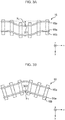
- Fig. 3A and Fig. 3B each illustrate one example of the alignment irregularity amount y R1 at the position of the wheel set 13a.
- Fig. 3A the case of the track 16 being the linear track will be explained as an example.
- Fig. 3B the case of the track 16 being the curved track will be explained as an example.
- 16a denotes a rail
- 16b denotes a crosstie.
- the alignment irregularity amount y R1 at the position of the wheel set 13a is a distance in the right and left direction between the contact position between the wheel 14a of the wheel set 13a and the rail 16a and the position of the rail 16a in the case where this position is assumed as a regular state.
- the position of the wheel set 13a is the contact position between the wheel 14a of the wheel set 13a and the rail 16a.
- the alignment irregularity amounts Y R2 , Y R3 , and y R4 at the positions of the wheel sets 13b, 13c, and 13d are also defined in the same manner as the alignment irregularity amount y R1 at the position of the wheel set 13a.
- m T is the mass of the bogies 12a, 12b.
- y t1 ⁇ ⁇ is acceleration of the bogie 12a in the right and left direction.
- c' 2 is a damping constant of a lateral movement damper.
- h 4 is a distance between the center of gravity of the bogie 12a and the lateral movement damper in the up and down direction.
- y b ⁇ is a velocity of the vehicle body 11 in the right and left direction.
- L represents 1/2 of the interval between the center of the bogie 12a and the center of the bogie 12b in the forward and backward direction (the interval between the center of the bogie 12a and the center of the bogie 12b in the forward and backward direction becomes 2L).
- ⁇ b ⁇ is an angular velocity of the vehicle body 11 in the yawing direction.
- h 5 is a distance between the lateral movement damper and the center of gravity of the vehicle body 11 in the up and down direction.
- ⁇ b ⁇ is an angular velocity of the vehicle body 11 in the rolling direction.
- y w2 ⁇ is a velocity of the wheel set 13b in the right and left direction.
- k' 2 is a spring constant of the air spring (bolster spring) in the right and left direction.
- h 2 is a distance between the center of gravity of each of the bogies 12a, 12b and the center of the air spring (bolster spring) in the up and down direction.
- y b is a displacement of the vehicle body 11 in the right and left direction.
- ⁇ b is a pivot amount (angular displacement) of the vehicle body 11 in the yawing direction.
- h 3 is a distance between the center of the air spring (bolster spring) and the center of gravity of the vehicle body 11 in the up and down direction.
- ⁇ b is a pivot amount (angular displacement) of the vehicle body 11 in the rolling direction.
- I Tz is a moment of inertia of the bogies 12a, 12b in the yawing direction.
- ⁇ t1 ⁇ ⁇ is angular acceleration of the bogie 12a in the yawing direction.
- ⁇ w2 ⁇ is an angular velocity of the wheel set 13b in the yawing direction.
- ⁇ w2 is a pivot amount (angular displacement) of the wheel set 13b in the yawing direction.
- y w2 is a displacement of the wheel set 13b in the right and left direction.
- k' 0 is stiffness of a rubber bush of the yaw damper.
- b' 0 represents 1/2 of the interval between the two yaw dampers, which are disposed on the right and left sides of each of the bogies 12a, 12b, in the right and left direction (the interval between the two yaw dampers, which are disposed on the right and left sides of each of the bogies 12a, 12b, in the right and left direction becomes 2b' 0 ).
- ⁇ y1 is a pivot amount (angular displacement) of the yaw damper disposed on the bogie 12a in the yawing direction.
- k'' 2 is a spring constant of the air spring (bolster spring) in the right and left direction.
- b 2 represents 1/2 of the interval between the two air springs (bolster springs), which are disposed on the right and left sides of each of the bogies 12a, 12b, in the right and left direction (the interval between the two air springs (bolster springs), which are disposed on the right and left sides of each of the bogies 12a, 12b, in the right and left direction becomes 2b 2 ).
- respective variables in (12) Equation are represented by being replaced with the variables in (11) Equation according to the meanings of the aforementioned subscripts.
- I Tx is a moment of inertia of the bogies 12a, 12b in the rolling direction.
- ⁇ t1 ⁇ ⁇ is angular acceleration of the bogie 12a in the rolling direction.
- c 1 is a damping constant of an axle damper in the up and down direction.
- b' 1 represents 1/2 of the interval between the two axle dampers, which are disposed on the right and left sides of each of the bogies 12a, 12b, in the right and left direction (the interval between the two axle dampers, which are disposed on the right and left sides of each of the bogies 12a, 12b, in the right and left direction becomes 2b' 1 ).
- c 2 is a damping constant of the air spring (bolster spring) in the up and down direction.
- ⁇ a1 ⁇ is an angular velocity of the air spring (bolster spring) disposed on the bogie 12a in the rolling direction.
- k 1 is a spring constant of an axle spring in the up and down direction.
- ⁇ is a value obtained by dividing the volume of the air spring (bolster spring) main body by the volume of an auxiliary air chamber.
- k 2 is a spring constant of the air spring (bolster spring) in the up and down direction.
- ⁇ a1 is a pivot amount (angular displacement) of the air spring (bolster spring) disposed on the bogie 12a in the rolling direction.
- k 3 is equivalent stiffness by a change in effective pressure receiving area of the air spring (bolster spring).
- ⁇ a2 is a pivot amount (angular displacement) of the air spring (bolster spring) disposed on the bogie 12b in the rolling direction.
- m B is the mass of the bogies 12a, 12b.
- y b ⁇ ⁇ is acceleration of the vehicle body 11 in the right and left direction.
- y t2 ⁇ is a velocity of the bogie 12b in the right and left direction.
- ⁇ t2 ⁇ is an angular velocity of the bogie 12b in the rolling direction.
- y t2 is a displacement of the bogie 12b in the right and left direction.
- ⁇ t2 is a pivot amount (angular displacement) of the bogie 12b in the rolling direction.
- I Bz is a moment of inertia of the vehicle body 11 in the yawing direction.
- ⁇ b ⁇ ⁇ is angular acceleration of the vehicle body 11 in the yawing direction.
- c 0 is a damping constant of the yaw damper in the forward and backward direction.
- ⁇ y1 ⁇ is an angular velocity of the yaw damper disposed on the bogie 12a in the yawing direction.
- ⁇ y2 ⁇ is an angular velocity of the yaw damper disposed on the bogie 12b in the yawing direction.
- ⁇ t2 is a pivot amount (angular displacement) of the bogie 12b in the yawing direction.
- I Bx is a moment of inertia of the vehicle body 11 in the rolling direction.
- ⁇ b ⁇ ⁇ is angular acceleration of the vehicle body 11 in the rolling direction.
- ⁇ y2 is a pivot amount (angular displacement) of the yaw damper disposed on the bogie 12b in the yawing direction.
- ⁇ a2 ⁇ is an angular velocity of the air spring (bolster spring) disposed on the bogie 12b in the rolling direction.
- In-phase components of the longitudinal creep force in one wheel of right and left wheels in one wheel set and the longitudinal creep force in the other wheel are components corresponding to a braking force and a driving force. Accordingly, the forward-and-backward-direction force is preferably determined so as to correspond to an opposite-phase component of the longitudinal creep force.
- the opposite-phase component of the longitudinal creep force is a component to be opposite in phase to each other between the longitudinal creep force in one wheel of the right and left wheels in one wheel set and the longitudinal creep force in the other wheel. That is, the opposite-phase component of the longitudinal creep force is a component, of the longitudinal creep force, in the direction in which the axle is twisted.
- the forward-and-backward-direction force becomes a component opposite in phase to each other out of forward-and-backward-direction components of forces to occur in the aforementioned two members attached to both the right and left sides of one wheel set.
- the axle box suspension being a mono-link type axle box suspension
- the axle box suspension includes a link
- the axle box and the bogie frame are coupled by the link.
- a rubber bush is attached to both ends of the link.
- the forward-and-backward-direction force becomes, out of forward-and-backward-direction components of loads that two links, which are attached to right and left ends of one wheel set one by one, receive, the component to be opposite in phase to each other.
- the link mainly receives, out of loads in the forward and backward direction, the right and left direction, and the up and down direction, the load in the forward and backward direction. Accordingly, one strain gauge only needs to be attached to each link, for example.
- the forward-and-backward-direction component of the load that this link receives is derived, to thereby obtain a measured value of the forward-and-backward-direction force.
- a forward-and-backward-direction displacement of the rubber bush attached to the link may be measured by a displacement meter.
- the product of a measured displacement and a spring constant of this rubber bush is set as the measured value of the forward-and-backward-direction force.
- the axle box suspension being the mono-link type axle box suspension
- the previously-described member for supporting the axle box becomes the link or the rubber bush.
- the load measured by the strain gauge attached to the link not only the component in the forward and backward direction, but also at least one component of a component in the right and left direction and a component in the up and down direction is sometimes contained.
- the load of the component in the right and left direction and the load of the component in the up and down direction that the link receives are sufficiently smaller than the load of the component in the forward and backward direction. Accordingly, only attaching one strain gauge to each link makes it possible to obtain a measured value of the forward-and-backward-direction force, which has accuracy to be required practically.
- the components other than the component in the forward and backward direction are sometimes included in the measured value of the forward-and-backward-direction force.
- three or more strain gauges may be attached to each link so as to cancel the strains in the up and down direction and the right and left direction. This makes it possible to improve the accuracy of the measured value of the forward-and-backward-direction force.
- the axle box suspension being an axle beam type axle box suspension
- the axle box suspension includes an axle beam
- the axle box and the bogie frame are coupled by the axle beam.
- the axle beam may be formed integrally with the axle box.
- a rubber bush is attached to a bogie frame-side end of the axle beam.
- the forward-and-backward-direction force becomes, out of forward-and-backward-direction components of loads that two axle beams, which are attached to right and left ends of one wheel set one by one, receive, the component to be opposite in phase to each other.
- the axle beam is likely to receive, out of loads in the forward and backward direction, the right and left direction, and the up and down direction, the load in the right and left direction, in addition to the load in the forward and backward direction.
- two or more strain gauges are attached to each axle beam so as to cancel the strain in the right and left direction, for example.
- the forward-and-backward-direction component of the load that the axle beam receives is derived, to thereby obtain a measured value of the forward-and-backward-direction force.
- a forward-and-backward-direction displacement of the rubber bush attached to the axle beam may be measured by a displacement meter.
- the product of a measured displacement and a spring constant of this rubber bush is set as the measured value of the forward-and-backward-direction force.
- the axle box suspension being the axle beam type axle box suspension
- the previously-described member for supporting the axle box becomes the axle beam or the rubber bush.
- the load measured by the strain gauge attached to the axle beam not only the components in the forward and backward direction and the right and left direction, but also the component in the up and down direction is sometimes included.
- the load of the component in the up and down direction that the axle beam receives is sufficiently smaller than the load of the component in the forward and backward direction and the load of the component in the right and left direction. Accordingly, unless the strain gauge is attached so as to cancel the load of the component in the up and down direction that the axle beam receives, a measured value of the forward-and-backward-direction force, which has accuracy to be required practically, can be obtained.
- the components other than the component in the forward and backward direction are sometimes included in the measured forward-and-backward-direction force, and three or more strain gauges may be attached to each axle beam so as to cancel the strain in the up and down direction as well as the strain in the right and left direction. This makes it possible to improve the accuracy of the measured value of the forward-and-backward-direction force.
- the axle box suspension being a leaf spring type axle box suspension
- the axle box suspension includes a leaf spring
- the axle box and the bogie frame are coupled by the leaf spring.
- a rubber bush is attached to ends of the leaf spring.
- the forward-and-backward-direction force becomes, out of forward-and-backward-direction components of loads that two leaf springs, which are attached to right and left ends of one wheel set one by one, receive, the component to be opposite in phase to each other.
- the leaf spring is likely to receive, out of loads in the forward and backward direction, the right and left direction, and the up and down direction, the load in the right and left direction and the load in the up and down direction, in addition to the load in the forward and backward direction.
- three or more strain gauges are attached to each leaf spring so as to cancel the strains in the right and left direction and the up and down direction, for example.
- the forward-and-backward-direction component of the load that the leaf spring receives is derived, to thereby obtain a measured value of the forward-and-backward-direction force.
- a forward-and-backward-direction displacement of the rubber bush attached to the leaf spring may be measured by a displacement meter.
- the product of a measured displacement and a spring constant of this rubber bush is set as the measured value of the forward-and-backward-direction force.
- the axle box suspension being the leaf spring type axle box suspension
- the previously-described member for supporting the axle box becomes the leaf spring or the rubber bush.
- the forward-and-backward-direction force has been explained here by taking the case of the system of the axle box suspension being a mono-link type, an axle beam type, and a leaf spring type as an example.
- the system of the axle box suspension is not limited to the mono-link type, the axle beam type, and the leaf spring type.
- the forward-and-backward-direction force can be determined in the same manner as in the mono-link type, the axle beam type, and the leaf spring type.
- the railway vehicle illustrated in Fig. 1 has the four wheel sets 13a to 13d. Accordingly, it is possible to obtain measured values of four forward-and-backward-direction forces T 1 to T 4 .
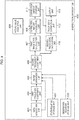
- Fig. 4 is a diagram illustrating one example of a functional configuration of an inspection apparatus 400.
- Fig. 5 is a diagram illustrating one example of a hardware configuration of the inspection apparatus 400.
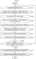
- Fig. 6 is a flowchart illustrating one example of first preprocessing in the inspection apparatus 400.
- the first preprocessing is processing for setting state equations and observation equations used in second preprocessing and main processing.
- Fig. 7 is a flowchart illustrating one example of the second preprocessing in the inspection apparatus 400.
- the second preprocessing is processing to derive a correction amount for an estimated value of the previously-described alignment irregularity amount after the first preprocessing is finished.
- Fig. 8 is a flowchart illustrating one example of the main processing in the inspection apparatus 400.
- the main processing is processing to derive an estimated value of a final alignment irregularity amount after the first preprocessing and the second preprocessing are finished.
- the inspection apparatus 400 is mounted on the railway vehicle.
- the railway vehicle is set the same as the railway vehicle with the inspection apparatus 400 mounted thereon.
- the inspection apparatus 400 includes, as its functions, a state equation storage unit 401, an observation equation storage unit 402, a data acquisition unit 403, a first frequency adjustment unit 404, a filter operation unit 405, a second frequency adjustment unit 406, a first track state calculation unit 407, an actual value acquisition unit 408, a correction amount calculation unit 409, a correction amount storage unit 410, a second track state calculation unit 411, a track state correction unit 412, and an output unit 413.
- the inspection apparatus 400 includes a CPU 501, a main memory 502, an auxiliary memory 503, a communication circuit 504, a signal processing circuit 505, an image processing circuit 506, an I/F circuit 507, a user interface 508, a display 509, and a bus 510.
- the CPU 501 overall controls the entire inspection apparatus 400.
- the CPU 501 uses the main memory 502 as a work area to execute a program stored in the auxiliary memory 503.
- the main memory 502 stores data temporarily.
- the auxiliary memory 503 stores various data, in addition to programs to be executed by the CPU 501.
- the auxiliary memory 503 stores state equations, observation equations, and correction amounts (a first correction amount, a second correction amount) to be described later.
- the state equation storage unit 401, the observation equation storage unit 402, and the correction amount storage unit 410 are fabricated by using the CPU 501 and the auxiliary memory 503, for example.
- the communication circuit 504 is a circuit intended for performing communication with the outside of the inspection apparatus 400.
- the communication circuit 504 receives information of the measured value of the forward-and-backward-direction force and pieces of information of measured values of accelerations of the vehicle body 11, the bogies 12a, 12b, and the wheel sets 13a to 13d in the right and left direction, for example.
- the communication circuit 504 may perform radio communication or wire communication with the outside of the inspection apparatus 400.
- the communication circuit 504 is connected to an antenna provided on the railway vehicle in the case of performing radio communication.
- the signal processing circuit 505 performs various pieces of signal processing on signals received in the communication circuit 504 and signals input according to the control by the CPU 501.
- the data acquisition unit 403 and the actual value acquisition unit 408 are fabricated by using the CPU 501, the communication circuit 504, and the signal processing circuit 505, for example.
- the first frequency adjustment unit 404, the filter operation unit 405, the second frequency adjustment unit 406, the first track state calculation unit 407, the correction amount calculation unit 409, the second track state calculation unit 411, and the track state correction unit 412 are fabricated by using the CPU 501 and the signal processing circuit 505, for example.
- the image processing circuit 506 performs various pieces of image processing on signals input according to the control by the CPU 501.
- the signal that has been subjected to the image processing is output on the display 509.
- the user interface 508 is a part through which an operator gives an instruction to the inspection apparatus 400.
- the user interface 508 includes buttons, switches, dials, and so on, for example. Further, the user interface 508 may include a graphical user interface using the display 509.
- the display 509 displays an image based on a signal output from the image processing circuit 506.
- the I/F circuit 507 exchanges data with a device connected to the I/F circuit 507.
- the user interface 508 and the display 509 are illustrated.
- the device to be connected to the I/F circuit 507 is not limited to these.
- a portable storage medium may be connected to the I/F circuit 507.
- at least a part of the user interface 508 and the display 509 may be provided outside the inspection apparatus 400.
- the output unit 413 is fabricated by using the communication circuit 504, the signal processing circuit 505, and at least any one of the image processing circuit 506, the I/F circuit 507, and the display 509, for example.
- the CPU 501, the main memory 502, the auxiliary memory 503, the signal processing circuit 505, the image processing circuit 506, and the I/F circuit 507 are connected to the bus 510. Communication among these components is performed via the bus 510. Further, the hardware of the inspection apparatus 400 is not limited to the one illustrated in Fig. 5 as long as it can perform later-described functions of the inspection apparatus 400.
- the state equation storage unit 401 stores state equations.
- the case of using the state equations described in Patent Literature 1 will be explained as an example.
- the motion equations that describe the yawings of the wheel sets 13a to 13d of (5) Equation to (8) Equation are not included in the state equation, and the state equation is constituted as follows.
- the forward-and-backward-direction forces T 1 to T 4 of the wheel sets 13a to 13d are expressed by (22) Equation to (25) Equation below.
- the forward-and-backward-direction forces T 1 to T 4 are determined according to the differences between the angular displacements ⁇ w1 to ⁇ w4 of the wheel sets in the yawing direction and the angular displacements ⁇ t1 to ⁇ t2 of the bogies on which these wheel sets are provided in the yawing direction.
- T 1 C wx b 1 2 ⁇ ⁇ t 1 ⁇ ⁇ ⁇ w 1 + K wx b 1 2 ⁇ t 1 ⁇ ⁇ w 1
- T 2 C wx b 1 2 ⁇ ⁇ t 1 ⁇ ⁇ ⁇ w 2 + K wx b 1 2 ⁇ t 1 ⁇ ⁇ w 2
- T 3 C wx b 1 2 ⁇ ⁇ t 2 ⁇ ⁇ ⁇ w 3 + K wx b 1 2 ⁇ t 2 ⁇ w 3
- T 4 C wx b 1 2 ⁇ ⁇ t 2 ⁇ ⁇ ⁇ w 4 + K wx b 1 2 ⁇ t 2 ⁇ ⁇ w 4
- Transformation variables e 1 to e 4 are defined as in (26) Equation to (29) Equation below. As above, the transformation variables e 1 to e 4 are defined by the differences between the angular displacements ⁇ t1 to ⁇ t2 of the bogies in the yawing direction and the angular displacements ⁇ w1 to ⁇ w4 of the wheel sets in the yawing direction. The transformation variables e 1 to e 4 are variables for performing mutual transformation between the angular displacements ⁇ t1 to ⁇ t2 of the bogies in the yawing direction and the angular displacements ⁇ w1 to ⁇ w4 of the wheel sets in the yawing direction.
- Equation to (33) Equation below are obtained.
- Equation to (33) Equation are substituted into the motion equations that describe the transversal vibrations of the wheel sets 13a to 13d (motion in the right and left direction) of (1) Equation to (4) Equation, (34) Equation to (37) Equation below are obtained.
- the motion equations that describe the transversal vibrations of the wheel sets 13a to 13d (motion in the right and left direction) of (1) Equation to (4) Equation are expressed by using the transformation variables e 1 to e 4 , thereby making it possible to eliminate the pivot amounts (angular displacements) ⁇ w1 to ⁇ w4 of the wheel sets 13a to 13d in the yawing direction that are included in these motion equations.
- the motion equations that describe the yawings of the bogies 12a, 12b of (11) Equation and (12) Equation are expressed by using the forward-and-backward-direction forces T 1 to T 4 , thereby making it possible to eliminate the angular displacements ⁇ w1 to ⁇ w4 and the angular velocities ⁇ w1 ⁇ to ⁇ w4 ⁇ of the wheel sets 13a to 13d in the yawing direction that are included in these motion equations.
- Equation to (37) Equation the motion equations that describe the transversal vibrations of the wheel sets 13a to 13d (motion in the right and left direction) are expressed, and at the same time, as in (38) Equation and (39) Equation, the motion equations that describe the yawings of the bogies 12a, 12b are expressed, and by using these, the state equation is constituted.
- Equation to (43) Equation are ordinary differential equations, and actual values of the transformation variables e 1 to e 4 , which are solutions of the equations, can be derived by using the values of the forward-and-backward-direction forces T 1 to T 4 in the wheel sets 13a to 13d.
- the values of the forward-and-backward-direction forces T 1 to T 4 are that a signal strength of a low-frequency component to be generated due to the railway vehicle traveling on the curved portion of the track is reduced from the time-series data of the measured value of the forward-and-backward-direction force by the later-described first frequency adjustment unit 404.
- the values of the transformation variables e 1 to e 4 derived as above are given to (34) Equation to (37) Equation. Further, the values of the forward-and-backward-direction forces T 1 to T 4 in the wheel sets 13a to 13d are given to (38) Equation and (39) Equation.
- the values of the forward-and-backward-direction forces T 1 to T 4 are that a signal strength of a low-frequency component to be generated due to the railway vehicle traveling on the curved portion of the track is reduced from the time-series data of the measured value of the forward-and-backward-direction force by the later-described first frequency adjustment unit 404.
- the state equation storage unit 401 receives the state equation constituted as above, for example, based on the operation of the user interface 508 by an operator and stores it.
- the observation equation storage unit 402 stores observation equations.
- the acceleration of the vehicle body 11 in the right and left direction, the accelerations of the bogies 12a, 12b in the right and left direction, and the accelerations of the wheel sets 13a to 13d in the right and left direction are set to observation variables.
- These observation variables are observation variables of filtering by a later-described Kalman filter.
- the motion equations that describe the transversal vibrations of (34) Equation to (37) Equation, (9) Equation, (10) Equation, and (15) Equation are used to constitute an observation equation.
- the observation equation storage unit 402 receives the observation equation constituted in this manner, for example, based on the operation of the user interface 508 by an operator and stores it.
- the data acquisition unit 403, the first frequency adjustment unit 404, the filter operation unit 405, the second frequency adjustment unit 406, the first track state calculation unit 407, the actual value acquisition unit 408, the correction amount calculation unit 409, and the correction amount storage unit 410 start. That is, after the first preprocessing by the flowchart in Fig. 6 is finished, the second preprocessing by the flowchart in Fig. 7 starts.
- the data acquisition unit 403 acquires measured data with a predetermined sampling period.
- the data acquisition unit 403 acquires, as the measured data, time-series data of a measured value of the acceleration of the vehicle body 11 in the right and left direction, time-series data of measured values of the accelerations of the bogies 12a, 12b in the right and left direction, and time-series data of measured values of the accelerations of the wheel sets 13a to 13d in the right and left direction.
- the respective accelerations are measured by using strain gauges attached to, for example, the vehicle body 11, the bogies 12a, 12b, and the wheel sets 13a to 13d respectively and an arithmetic device that calculates the accelerations by using measured values of these strain gauges.
- the measurement of the accelerations can be performed by a well-known technique, and thus its detailed explanation is omitted.
- the data acquisition unit 403 acquires, as the measured data, time-series data of the measured value of the forward-and-backward-direction force.
- the method of measuring the forward-and-backward-direction force is as described previously.
- the data acquisition unit 403 can acquire the measured data by performing communication with the previously-described arithmetic device, for example. At Step S701, the data acquisition unit 403 acquires measured data in the entire traveling section of the railway vehicle.
- the first frequency adjustment unit 404 reduces (preferably removes) the signal strength of the low-frequency component contained in the time-series data of the measured value of the forward-and-backward-direction force (a second physical quantity) out of the measured data acquired by the data acquisition unit 403.
- a signal of this low-frequency component is a signal that is not measured when the railway vehicle is traveling on the linear track, but is measured when the railway vehicle is traveling on the curved track. That is, the signal measured when the railway vehicle is traveling on the curved track can be regarded as a signal obtained by superimposing the signal of this low-frequency component on the signal measured when the railway vehicle is traveling on the linear track.
- the present inventors devised a model in which an AR (Auto-regressive) model is corrected. Then, the present inventors devised reducing the signal strength of the low-frequency component contained in the time-series data of the measured value of the forward-and-backward-direction force by using this model.
- the model devised by the present inventors is referred to as a corrected AR model.
- the well-known AR model is referred to as an AR model simply.
- a value of time-series data y of a physical quantity at a time k (1 ⁇ k ⁇ M) is set to y k .
- M is a number indicating, as the time-series data y of the physical quantity, data until when are contained, and is preset.
- the time-series data of the physical quantity will be abbreviated to data y as necessary.
- the AR model approximating the value y k of the data y is as in (45) Equation below, for example.
- the AR model is, as illustrated in (45) Equation, an equation expressing a predicted value y ⁇ k of the physical quantity at the time k (m + 1 ⁇ k ⁇ M) in the data y by using an actual value y k - 1 of the physical quantity at a time k - 1 (1 ⁇ 1 ⁇ m) prior to the time k in the data y.
- y ⁇ k is expressed by adding ⁇ above y k in (45) Equation.
- ⁇ is a coefficient of the AR model.
- m is a number of the value of the data y to be used for approximating the value y k of the data y at the time k in the AR model, and is a number among values y k - 1 to y k - m of the data y at continuous times k - 1 to k - m prior to the time k.
- m is an integer less than M. As m, for example, 1500 can be used.
- conditional expression for approximating the predicted value y ⁇ k of the physical quantity at the time k by the AR model to the value y k by using a least square method As the condition for approximating the predicted value y ⁇ k of the physical quantity at the time k by the AR model to the value y k , it is possible to employ a condition that minimizes a square error between the predicted value y ⁇ k of the physical quantity at the time k by the AR model and the value y k , for example. That is, the least square method is used in order to approximate the predicted value y ⁇ k of the physical quantity at the time k by the AR model to the value y k .
- Equation below is a conditional expression for minimizing the square error between the predicted value y ⁇ k of the physical quantity at the time k by the AR model and the value y k .
- R jl in (48) Equation is called autocorrelation of the data y, and is a value defined by (49) Equation below.
- at this time is referred to as a time lag.
- Equation is an equation derived from a condition that minimizes the error between the predicted value y ⁇ k of the physical quantity at the time k by the AR model and the value y k of the physical quantity at the time k corresponding to the predicted value y ⁇ k .
- Equation is called a Yule-Walker equation.
- (50) Equation is a linear equation in which a vector composed of coefficients of the AR model is set to a variable vector.
- a constant vector on the left side in (50) Equation is a vector whose component is the autocorrelation of the data y with a time lag of 1 to m.
- a coefficient matrix on the right side in (50) Equation is a matrix whose component is the autocorrelation of the data y with a time lag of 0 to m - 1.
- the coefficient matrix on the right side in (50) Equation is referred to as an autocorrelation matrix as necessary.
- the present inventors focused on the autocorrelation matrix R to be multiplied by the coefficient ⁇ of the AR model and earnestly examined it. As a result, the present inventors found out that it is possible to reduce the effect of a high-frequency component contained in the data y by using a part of eigenvalues of the autocorrelation matrix R. That is, the present inventors found out that it is possible to rewrite the autocorrelation matrix R so that the low-frequency component is emphasized.
- the diagonal matrix ⁇ in (52) Equation is a matrix whose diagonal component is the eigenvalues of the autocorrelation matrix R as illustrated in (53) Equation below.
- the diagonal component of the diagonal matrix ⁇ is set to ⁇ 11 , ⁇ 22 , ⁇ , ⁇ mm .
- the orthogonal matrix U is a matrix in which each column component vector is an eigenvector of the autocorrelation matrix R.
- the column component vector of the diagonal matrix U is set to u 1 , u 2 , ⁇ , u m .
- the eigenvalue of the autocorrelation matrix R responsive to an eigenvector u j is ⁇ jj .
- the eigenvalue of the autocorrelation matrix R is a variable reflecting the strength of each frequency component included in a time waveform of the predicted value y ⁇ k of the physical quantity at the time k by the AR model.
- ⁇ ⁇ 11 0 0 0 ⁇ 0 0 ⁇ mm
- U u 1 u 2 ⁇ u m
- ⁇ 11 , ⁇ 22 , ⁇ , ⁇ mm being the diagonal components of the diagonal matrix ⁇ obtained by the result of the singular value decomposition of the autocorrelation matrix R are set in descending order in order to simplify the illustration of the mathematical equation.
- a matrix R' is defined as in (54) Equation below by using, out of the eigenvalues of the autocorrelation matrix R illustrated in (53) Equation, s pieces of the eigenvalues, which are chosen from the largest.
- s is a number that is 1 or more and less than m. In this embodiment, s is preset.
- a matrix U s in (54) Equation is a matrix of m ⁇ s composed of s pieces of the column component vectors (eigenvectors corresponding to the eigenvalues to be used), which are chosen from the left of the orthogonal matrix U of (52) Equation. That is, the matrix U s is a submatrix composed of the left elements of m ⁇ s cut out from the orthogonal matrix U. Further, U s T in (54) Equation is a transposed matrix of U s . U s T is a matrix of s ⁇ m composed of s pieces of row component vectors, which are chosen from the top of the matrix U T in (52) Equation.
- the matrix ⁇ s in (54) Equation is a matrix of s ⁇ s composed of s pieces of columns, which are chosen from the left, and s pieces of rows, which are chosen from the top, of the diagonal matrix ⁇ in (52) Equation. That is, the matrix ⁇ s is a submatrix composed of the top and left elements of s ⁇ s cut out from the diagonal matrix ⁇ .
- Equation is modified, and thereby (57) Equation below is obtained as the equation deriving the coefficient ⁇ .
- the model that calculates the predicted value y ⁇ k of the physical quantity at the time k from (45) Equation while using the coefficient ⁇ derived by (57) Equation is the "corrected AR model.”
- [Mathematical equation 30] ⁇ 1 ⁇ 2 ⁇ ⁇ m U s ⁇ s ⁇ 1 U s T R 10 R 20 ⁇ R m 0
- the matrix U s is not the submatrix composed of the left elements of m ⁇ s cut out from the orthogonal matrix U, but becomes a submatrix composed of the cut out column component vectors corresponding to the eigenvalues to be used (the eigenvectors).
- the matrix ⁇ s is not the submatrix composed of the top and left elements of s ⁇ s cut out from the diagonal matrix ⁇ , but becomes a submatrix to be cut out so as to make the eigenvalues used for determining the coefficient of the corrected AR model become the diagonal components.
- the matrix U s in (57) Equation is an equation to be used for determining the coefficient of the corrected AR model.
- the matrix U s in (57) Equation is a matrix (a third matrix) in which the eigenvectors corresponding to the eigenvalues used for determining the coefficient of the corrected AR model are set to the column component vectors, which is the submatrix of the orthogonal matrix U obtained by the singular value decomposition of the autocorrelation matrix R.
- the matrix ⁇ s in (57) Equation is a matrix (a second matrix) in which the eigenvalues used for determining the coefficient of the corrected AR model are set to the diagonal components, which is the submatrix of the diagonal matrix obtained by the singular value decomposition of the autocorrelation matrix R.
- the matrix U s ⁇ s U s T in (57) Equation is a matrix (a first matrix) derived from the matrix ⁇ s and the matrix U s .
- the right side of (57) Equation is calculated, and thereby the coefficient ⁇ of the corrected AR model is derived.
- One example of the method of deriving the coefficient ⁇ of the corrected AR model has been explained above.
- the method of deriving the coefficient of the AR model to be the base of the corrected AR model the method of using the least square method for the predicted value y ⁇ k of the physical quantity at the time k has been set in order to make the method understandable intuitively.
- a method of defining the AR model by using the concept of a stochastic process and deriving its coefficient generally. In this case, the autocorrelation is expressed by autocorrelation of the stochastic process (a population).
- This autocorrelation of the stochastic process is expressed as a function of a time lag.
- the autocorrelation of the data y in this embodiment may be replaced with a value calculated by another calculating formula as long as it approximates the autocorrelation of the stochastic process.
- R 22 to R mm are autocorrelation with a time lag of 0 (zero), but they may be replaced with R 11 .
- the number s of the eigenvalues extracted from the autocorrelation matrix R illustrated in (53) Equation can be determined from a distribution of the eigenvalues of the autocorrelation matrix R, for example.
- the forward-and-backward-direction force is applied here.
- the value of the forward-and-backward-direction force varies according to the state of the railway vehicle.
- the railway vehicle is first made to travel on the track 16 to obtain the data y of the measured value of the forward-and-backward-direction force.
- the autocorrelation matrix R is derived by using (49) Equation and (51) Equation for each of the obtained data y.
- the autocorrelation matrix R is subjected to singular value decomposition expressed by (52) Equation, to thereby derive the eigenvalues of the autocorrelation matrix R.
- FIG. 9 is a view illustrating one example of the distribution of the eigenvalues of the autocorrelation matrix R.
- eigenvalues ⁇ 11 to ⁇ mm which are obtained by the autocorrelation matrix R in each of the data y of the measured value of the forward-and-backward-direction force T 1 in the wheel set 13a being subjected to singular value decomposition, are aligned in ascending order and are plotted.
- the horizontal axis is an index of the eigenvalue and the vertical axis is the value of the eigenvalue.
- the example illustrated in Fig. 9 includes one eigenvalue having a value significantly higher than the others. Further, the example includes two eigenvalues that have a value relatively larger as compared to the others and are not regarded as 0 (zero), which are not as high as the aforementioned eigenvalue having a significantly higher value.
- the first frequency adjustment unit 404 performs the following processing by using the value y k of the data y of the measured value of the forward-and-backward-direction force at the time k acquired in the data acquisition unit 403.
- the first frequency adjustment unit 404 generates the autocorrelation matrix R using (49) Equation and (51) Equation based on the data y of the measured value of the forward-and-backward-direction force and preset numbers M, m.
- the first frequency adjustment unit 404 performs singular value decomposition on the autocorrelation matrix R, to thereby derive the orthogonal matrix U and the diagonal matrix ⁇ of (52) Equation, and derives the eigenvalues ⁇ 11 to ⁇ mm of the autocorrelation matrix R from the diagonal matrix ⁇ .
- the first frequency adjustment unit 404 chooses s pieces of the eigenvalues ⁇ 11 to ⁇ ss from the largest from among the plural eigenvalues ⁇ 11 to ⁇ mm of the autocorrelation matrix R as the eigenvalues of the autocorrelation matrix R to be used for deriving the coefficient ⁇ of the corrected AR model.
- the first frequency adjustment unit 404 determines the coefficient ⁇ of the corrected AR model using (57) Equation based on the data y of the measured value of the forward-and-backward-direction force, the eigenvalues ⁇ 11 to ⁇ ss , and the orthogonal matrix U obtained by the singular value decomposition of the autocorrelation matrix R.
- the first frequency adjustment unit 404 derives the predicted value y ⁇ k of the data y of the measured value of the forward-and-backward-direction force at the time k from (45) Equation based on the coefficient ⁇ of the corrected AR model and the data y of the measured value of the forward-and-backward-direction force.
- Time-series data of the predicted value y ⁇ k of the forward-and-backward-direction force result in the time-series data from which the low-frequency component contained in the data y of the measured value of the forward-and-backward-direction force has been extracted.
- Fig. 10 is a view illustrating one example of the time-series data of the measured value of the forward-and-backward-direction force (the measured value) and the time-series data of the predicted value of the forward-and-backward-direction force (the calculated value).
- the measured values of the four forward-and-backward-direction forces T 1 to T 4 are obtained. That is, four pieces of the data y of the forward-and-backward-direction force are obtained.
- the measured value and the calculated value of each of four pieces of the data y are illustrated.
- the vertical axis indicates the forward-and-backward-direction forces T 1 to T 4 (Nm).
- the calculated value of the forward-and-backward-direction force T 1 in the wheel set 13a is biased at about 15 seconds to 35 seconds (namely, a value larger than that at another time is exhibited). This period corresponds to the period when the wheel set 13a passes through the curved track.
- the calculated value of the forward-and-backward-direction force T 2 in the wheel set 13b, the calculated value of the forward-and-backward-direction force T 3 in the wheel set 13c, and the calculated value of the forward-and-backward-direction force T 4 in the wheel set 13d are also biased during the period when the wheel sets 13b, 13c, and 13d pass through the curved track similarly to the calculated value of the forward-and-backward-direction force T 1 in the wheel set 13a.
- the first frequency adjustment unit 404 subtracts the time-series data of the predicted value y ⁇ k of the forward-and-backward-direction force from the time-series data (the data y) of the measured value y k of the forward-and-backward-direction force.
- the time-series data resulting from the subtraction of the time-series data of the predicted value y ⁇ k of the forward-and-backward-direction force from the time-series data (the data y) of the measured value y k of the forward-and-backward-direction force are referred to as time-series data of a high-frequency component of the forward-and-backward-direction force as necessary.
- a value of the time-series data of the high-frequency component of the forward-and-backward-direction force at each sampling time is referred to as a value of the high-frequency component of the forward-and-backward-direction force as necessary.
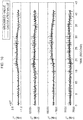
- Fig. 11 is a view illustrating one example of the time-series data of the high-frequency component of the forward-and-backward-direction force.
- the vertical axis in Fig. 11 indicates the time-series data of the high-frequency components of the forward-and-backward-direction forces T 1 , T 2 , T 3 , and T 4 . That is, the high-frequency components of the forward-and-backward-direction forces T 1 , T 2 , T 3 , and T 4 illustrated on the vertical axis in Fig.
- Fig. 11 are ones obtained by subtracting the calculated values from the measured values of the forward-and-backward-direction forces T 1 , T 2 , T 3 , and T 4 in the wheel sets 13a, 13b, 13c, and 13d that are illustrated in Fig. 10 respectively.
- the horizontal axis in Fig. 11 indicates a measuring time and a calculating time of the forward-and-backward-direction forces T 1 to T 4 , each of which is an elapsed time (second) from a reference time when the reference time is set to 0 (zero), similarly to the horizontal axis in Fig. 10 .
- the first frequency adjustment unit 404 derives the time-series data of the high-frequency components of the forward-and-backward-direction forces T 1 to T 4 as above.
- the filter operation unit 405 sets the observation equation as the observation equation stored by the observation equation storage unit 402, sets the state equation as the state equation stored by the state equation storage unit 401, and determines estimated values of the state variables illustrated in (44) Equation by the Kalman filter. At this time, the filter operation unit 405 uses, out of pieces of the measured data acquired in the data acquisition unit 403, the measured data excluding the forward-and-backward-direction forces T 1 to T 4 and the time-series data of the high-frequency components of the forward-and-backward-direction forces T 1 to T 4 generated in the first frequency adjustment unit 404.
- the measured value of the acceleration of the vehicle body 11 in the right and left direction the measured values of the accelerations of the bogies 12a, 12b in the right and left direction, and the measured values of the accelerations of the wheel sets 13a to 13d in the right and left direction are contained.
- the time-series data of the high-frequency components of the forward-and-backward-direction forces T 1 to T 4 generated in the first frequency adjustment unit 404 are used without using the measured data (the measured values) acquired in the data acquisition unit 403.
- the Kalman filter is one of the methods of performing data assimilation. That is, the Kalman filter is one example of the method to determine an estimated value of an unobserved variable (state variable) so as to make the difference between, of an observable variable (observation variable), a measured value and an estimated value small (minimum).
- the filter operation unit 405 derives a Kalman gain at which the difference between, of the observation variable, the measured value and the estimated value becomes small (minimum) and derives the estimated value of the unobserved variable (state variable) at that time.
- the following observation equation of (58) Equation and the following state equation of (59) Equation are used.
- Equation Y is a vector in which the measured value of the observation variable is stored. H is an observation model. X is a vector in which the state variable is stored. V is observation noise. In (59) Equation, X ⁇ indicates a time differentiation of X. ⁇ is a linear model. W is system noise. Incidentally, the Kalman filter itself can be fabricated by a well-known technique, and thus its detailed explanation is omitted.
- the filter operation unit 405 determines the estimated values of the state variables illustrated in (44) Equation with a predetermined sampling period, to thereby generate time-series data of the estimated values of the state variables illustrated in (44) Equation.
- the second frequency adjustment unit 406 reduces (preferably removes) the signal strength of the low-frequency component contained in the time-series data of the estimated values of the state variables (the second physical quantity) generated by the filter operation unit 405.
- the processing of the second frequency adjustment unit 406 is no longer required.
- the second frequency adjustment unit 406 uses the corrected AR model to reduce the signal strength of the low-frequency component contained in the time-series data of the estimated values of the state variables similarly to the first frequency adjustment unit 404.
- the second frequency adjustment unit 406 performs the following processing for each state variable with a predetermined sampling period.
- the state variable is applied here. That is, the data y of the state variable result in the time-series data of the estimated values of the state variables generated by the filter operation unit 405.
- the estimated values of the state variables each vary according to the state of the railway vehicle.
- the second frequency adjustment unit 406 generates the autocorrelation matrix R using (49) Equation and (51) Equation based on the data y of the estimated values of the state variables and the preset numbers M and m.
- the second frequency adjustment unit 406 performs singular value decomposition on the autocorrelation matrix R, to thereby derive the orthogonal matrix U and the diagonal matrix ⁇ of Equation (52), and derives the eigenvalues ⁇ 11 to ⁇ mm of the autocorrelation matrix R from the diagonal matrix ⁇ .
- the second frequency adjustment unit 406 chooses s pieces of the eigenvalues ⁇ 11 to ⁇ ss from the largest from among the plural eigenvalues ⁇ 11 to ⁇ mm of the autocorrelation matrix R as the eigenvalues of the autocorrelation matrix R to be used for deriving the coefficient ⁇ of the corrected AR model.
- s is preset for each state variable. For example, the railway vehicle is made to travel on the track 16, to then obtain the data y of the estimated value of each of the state variables in such a manner as explained so far. Then, a distribution of the eigenvalues of the autocorrelation matrix R is made individually for each state variable. From the distributions of the eigenvalues of the autocorrelation matrix R, the number s of the eigenvalues to be extracted from the autocorrelation matrix R illustrated in (53) Equation is determined for each of the state variables.
- the second frequency adjustment unit 406 determines the coefficient ⁇ of the corrected AR model using (57) Equation based on the data y of the estimated value of the state variable, the eigenvalues ⁇ 11 to ⁇ ss , and the orthogonal matrix U obtained by the singular value decomposition of the autocorrelation matrix R.
- the second frequency adjustment unit 406 derives the predicted value y ⁇ k of the data y of the estimated value of the state variable at the time k from (45) Equation based on the coefficient ⁇ of the corrected AR model and the data y of the estimated value of the state variable.
- Time-series data of the predicted value y ⁇ k of the state variable result in the time-series data from which the low-frequency component contained in the data y of the estimated value of the state variable has been extracted.
- the second frequency adjustment unit 406 subtracts the time-series data of the predicted value y ⁇ k of the state variable from the data y of the estimated value of the state variable.
- time-series data resulting from the subtraction of the time-series data of the predicted value y ⁇ k of the state variable from the data y of the estimated value of the state variable are referred to as time-series data of a high-frequency component of the state variable as necessary.
- Equation to (63) Equation are obtained.
- the first track state calculation unit 407 calculates estimated values of the pivot amounts (angular displacements) ⁇ w1 to ⁇ w4 of the wheel sets 13a to 13d in the yawing direction by (30) Equation to (33) Equation. Then, the first track state calculation unit 407 gives the estimated values of the pivot amounts (angular displacements) ⁇ w1 to ⁇ w4 of the wheel sets 13a to 13d in the yawing direction, the values of the high-frequency components of the state variables generated in the second frequency adjustment unit 406, and the values of the high-frequency components of the forward-and-backward-direction forces T 1 to T 4 generated in the first frequency adjustment unit 404 to (60) Equation to (63) Equation, to thereby calculate the alignment irregularity amounts y R1 to y R4 at the positions of the wheel sets 13a to 13d.
- the state variables to be used here are the displacements y t1 to y t2 of the bogies 12a, 12b in the right and left direction, the velocities y t1 ⁇ to y t2 ⁇ of the bogies 12a, 12b in the right and left direction, the displacements y w1 to y w4 of the wheel sets 13a to 13d in the right and left direction, and the velocities y w1 ⁇ to y w4 ⁇ of the wheel sets 13a to 13d in the right and left direction.
- the first track state calculation unit 407 performs such a calculation of the alignment irregularity amounts y R1 to y R4 as above with a predetermined sampling period, to thereby obtain the time-series data of the alignment irregularity amounts y R1 to y R4 .
- the first track state calculation unit 407 calculates an alignment irregularity amount y R from the alignment irregularity amounts y R1 to y R4 .
- the first track state calculation unit 407 matches phases of the time-series data of the alignment irregularity amounts y R2 to y R4 to a phase of the time-series data of the alignment irregularity amount y R1 . That is, the first track state calculation unit 407 calculates, from the distance between the wheel set 13a and the wheel sets 13b to 13d in the forward and backward direction and the velocity of the railway vehicle, a delay time between the time when the wheel set 13a passes through a certain position and the time when the wheel sets 13b to 13d pass through the certain position. The first track state calculation unit 407 displaces the phases of the time-series data of the alignment irregularity amounts y R2 to y R4 by this delay time.
- the first track state calculation unit 407 calculates an arithmetic mean value of the sum of the values of the alignment irregularity amounts y R1 to y R4 whose phases are matched at the same sampling time as the alignment irregularity amount y R at this sampling time.
- the first track state calculation unit 407 performs such a calculation at each sampling time, to thereby obtain time-series data of the alignment irregularity amount y R .
- the phases of the alignment irregularity amounts y R2 to y R4 are matched to the phase of the alignment irregularity amount y R1 , thereby making it possible to cancel disturbance factors existing in common in the time-series data of the alignment irregularity amounts y R1 to y R4 .
- the first track state calculation unit 407 may find a moving average of each of the alignment irregularity amounts y R1 to y R4 whose phases are matched (namely, pass each of the alignment irregularity amounts y R1 to y R4 through a low-pass filter) and calculate the alignment irregularity amount y R from the alignment irregularity amounts y R1 to y R4 whose moving averages have been found.
- the first track state calculation unit 407 may calculate, as the alignment irregularity amount y R , an arithmetic mean value of two of the values of the alignment irregularity amounts y R1 to y R4 whose phases are matched at the same sampling time from which the maximum value and the minimum value are removed.
- the inspection apparatus 400 uses the measured data at each sampling time acquired by the data acquisition unit 403 while the railway vehicle is traveling in the entire traveling section of the railway vehicle, to execute pieces of the processing of the first frequency adjustment unit 404, the filter operation unit 405, the second frequency adjustment unit 406, and the first track state calculation unit 407.
- the first track state calculation unit 407 can obtain the alignment irregularity amount y R at each sampling time while the railway vehicle is traveling in the entire traveling section.
- the first track state calculation unit 407 calculates a traveling position of the railway vehicle at each sampling time based on, for example, a traveling velocity of the railway vehicle and an elapsed time from the time when the railway vehicle starts to travel.
- the traveling position of the railway vehicle is the position of the wheel set 13a is explained as an example.
- the first track state calculation unit 407 calculates the alignment irregularity amount y R at each traveling position of the railway vehicle based on the alignment irregularity amount y R at each sampling time and the traveling position of the railway vehicle at each sampling time.
- the value calculated in this manner is referred to as an estimated value of the alignment irregularity amount at each position in the entire traveling section of the railway vehicle or an estimated value of the alignment irregularity amount as necessary.
- the first track state calculation unit 407 does not always need to calculate the traveling position of the railway vehicle at each sampling time as described previously.
- the first track state calculation unit 407 may derive the traveling position of the railway vehicle at each sampling time by using a GPS (Global Positioning System) .
- GPS Global Positioning System
- the actual value acquisition unit 408 acquires an actual measured value of the alignment irregularity amount at each position in the entire traveling section of the railway vehicle.
- the actual measured value of the alignment irregularity amount at each position in the entire traveling section of the railway vehicle is set to be measured before the second preprocessing is started.
- the timing for acquiring the actual measured value of the alignment irregularity amount at each position in the entire traveling section of the railway vehicle is not limited to a period between Step S705 and Step S707.
- the timing for acquiring the actual measured value of the alignment irregularity amount at each position in the entire traveling section of the railway vehicle may be any timing as long as it is the timing prior to Step S707.
- the actual value acquisition unit 408 may acquire the actual measured value of the alignment irregularity amount at each position in the entire traveling section of the railway vehicle before the flowchart in Fig. 7 is started.
- the actual measured value of the alignment irregularity amount at each position in the entire traveling section of the railway vehicle is referred to as an actual measured value of the alignment irregularity amount or an actual measured value as necessary.
- the actual measured value of the alignment irregularity amount is a value to be obtained by directly measuring the alignment irregularity amount.
- the actual measured value of the alignment irregularity amount can be obtained as follows, for example.
- a test vehicle provided with a sensor that directly measures the alignment irregularity amount is made to travel.
- the direct measurement of the alignment irregularity amount by the sensor during traveling of the test vehicle is performed repeatedly in a predetermined cycle, to thereby obtain the alignment irregularity amount in the entire traveling section of the railway vehicle.
- the actual measured value of the alignment irregularity amount can also be obtained by using the measuring device described in Patent Literature 2, for example.
- the actual measured value of the alignment irregularity amount can be obtained by a well-known technique. Thus, its detailed explanation is omitted here.
- Fig. 12A and Fig. 12B to Fig. 14A and Fig. 14B are views illustrating first to sixth examples of the relation between the estimated value of the alignment irregularity amount (y R ), the actual value of the alignment irregularity amount (y R ), the traveling velocity of the railway vehicle (v), and the curvature of the track 16 (rail) (1/R) and the distance from the starting point of the railway vehicle respectively.
- the estimated value of the alignment irregularity amount is the one calculated by the first track state calculation unit 407.
- the actual value of the alignment irregularity amount is the one acquired by the actual value acquisition unit 408.
- illustration of data of a portion where the distance from the starting point of the railway vehicle is small is omitted.
- graphs 1211, 1221, 1311, 1321, 1411, and 1421 each indicate the estimated value of the alignment irregularity amount calculated by the first track state calculation unit 407.
- Graphs 1212, 1222, 1312, 1322, 1412, and 1422 each indicate the actual value of the alignment irregularity amount acquired by the actual value acquisition unit 408.
- Graphs 1213, 1223, 1313, 1323, 1413, and 1423 each indicate the traveling velocity of the railway vehicle.
- Graphs 1214, 1224, 1314, 1324, 1414, and 1424 each indicate the curvature 1/R of the track 16 (rail).
- Fig. 12A and Fig. 12B illustrate that the graphs 1214 and 1224 are the same and the traveling sections are the same.
- Fig. 12A and Fig. 12B illustrate that the traveling velocities of the railway vehicle are different as illustrated in the graphs 1213, 1223. This reveals that due to the different traveling velocities of the railway vehicle in the same traveling section, as illustrated in the graphs 1211, 1221, the estimated values of the alignment irregularity amount are different but the difference is not so large.
- the graphs 1212 and 1222 are the same. As illustrated in the graphs 1211, 1212, it becomes clear that there is a difference between the estimated value of the alignment irregularity amount calculated by the first track state calculation unit 407 and the actual value of the alignment irregularity amount acquired by the actual value acquisition unit 408. The same is true of the graphs 1221, 1222.
- the traveling sections illustrated in Fig. 12A and Fig. 12B are a sharp curve with a curvature radius R of 171 m. Therefore, the railway vehicle is in flange contact with the track 16.
- Fig. 15 is a view explaining one example of the flange contact.
- Fig. 15 illustrates a cross section of the case where left and right rails of a track 16 and a single wheel set 13 are cut vertically to the traveling direction of a railway vehicle (x axis direction). Further, Fig. 15 illustrates a state of the wheel set 13 in the case where the track 16 (rail) is curved to the right (in the negative direction of the y axis) and the railway vehicle is traveling while curving to the right.
- Fig. 15 also illustrates a lateral creep force F y L i and a normal load N L i in a left wheel 14L and a lateral creep force F y R i and a normal load N R i in a right wheel 14R.
- the railway vehicle when traveling on the rail curved to the right, the railway vehicle receives an acting force in the left direction (the positive direction of the y axis) and the wheel set 13 moves to the left, and thereby reaction forces in the left and right direction from the contact position between the wheel 14L and the rail and the contact position between the wheel 14R and the rail increase to reach a force balance point.
- this acting force further increases, the wheel set 13 further moves to the left, and when a contact angle ⁇ L becomes the same as a flange angle a L of the left wheel 14L, the left wheel 14L is to come into contact with the rail at a flange, as illustrated in Fig. 15 .
- Such a contact is referred to as the flange contact.
- the right wheel 14R comes into contact with the rail at a tread.
- Fig. 13A and Fig. 13B illustrate that the graphs 1314 and 1324 are the same and the traveling sections are the same. As illustrated in the graphs 1314, 1324, the curvature 1/R is 0 (zero), and thus it becomes clear that the traveling sections illustrated in Fig. 13A and Fig. 13B are a linear track.
- Fig. 13A and Fig. 13B illustrate that the traveling velocities of the railway vehicle are different as illustrated in the graphs 1313, 1323. This reveals that due to the different traveling velocities of the railway vehicle in the same traveling section, as illustrated in the graphs 1311, 1321, the estimated values of the alignment irregularity amount are different but the difference is not so large. Further, in Fig. 13A and Fig.
- an S/N ratio of the measured value of the forward-and-backward-direction force decreases because the traveling velocity of the railway vehicle decreases to 30 km/h or less.
- a high-frequency noise is mixed into the estimated value of the alignment irregularity amount.
- a feature amount of the alignment irregularity amount (such as a way how the graph changes) is captured in the graphs 1311, 1321.
- the graphs 1312 and 1322 are the same. As illustrated in the graphs 1311, 1312, it becomes clear that there is a difference between the estimated value of the alignment irregularity amount calculated by the first track state calculation unit 407 and the actual value of the alignment irregularity amount acquired by the actual value acquisition unit 408. The same is true of the graphs 1321, 1322.
- Fig. 14A and Fig. 14B illustrate that the graphs 1414 and 1424 are the same and the traveling sections are the same.
- Fig. 14A and Fig. 14B illustrate that the traveling velocities of the railway vehicle are different as illustrated in the graphs 1413, 1423. This reveals that due to the different traveling velocities of the railway vehicle in the same traveling section, as illustrated in the graphs 1411, 1421, the estimated values of the alignment irregularity amount are different but the difference is not so large. Further, the graphs 1412 and 1422 (the actual values of the alignment irregularity amount) are the same.
- the traveling sections illustrated in Fig. 14A and Fig. 14B are a gentle curve with the curvature radius R of 993 m, and the railway vehicle does not come into flange contact with the track 16.
- the correction amount calculation unit 409 calculates, when the estimated value of the alignment irregularity amount at each position in the entire traveling section of the railway vehicle is calculated by the first track state calculation unit 407, a correction amount at each position in the entire traveling section of the railway vehicle.
- the correction amount at each position in the entire traveling section of the railway vehicle is the correction amount for the estimated value of the alignment irregularity amount at each position in the entire traveling section of the railway vehicle, which is calculated by the later-described second track state calculation unit 411.
- the correction amount calculation unit 409 calculates the correction amount at each position in the entire traveling section of the railway vehicle based on the estimated value of the alignment irregularity amount at each position in the entire traveling section of the railway vehicle that is calculated by the first track state calculation unit 407 and the actual measured value of the alignment irregularity amount at each position in the entire traveling section of the railway vehicle that is acquired by the actual value acquisition unit 408.
- the correction amount calculation unit 409 calculates the correction amount at each position in the entire traveling section of the railway vehicle as follows.
- the correction amount calculation unit 409 extracts a pair of values at the same position, which is a pair of the estimated value of the alignment irregularity amount that is calculated by the first track state calculation unit 407 and the actual measured value of the alignment irregularity amount that is acquired by the actual value acquisition unit 408.
- the correction amount calculation unit 409 calculates, as the correction amount at the position, a value obtained by subtracting the extracted actual measured value of the alignment irregularity amount from the extracted estimated value of the alignment irregularity amount.
- the correction amount calculation unit 409 performs such a calculation of the correction amount by using the estimated value of the alignment irregularity amount and the actual measured value of the alignment irregularity amount at each position in the entire traveling section of the railway vehicle. In this manner, the correction amount at each position in the entire traveling section of the railway vehicle is calculated.
- the correction amount calculation unit 409 calculates one set of correction amounts at all the positions in the entire traveling section of the railway vehicle (Step S707).
- the correction amount calculation unit 409 performs interpolation processing on the correction amount at each position in the entire traveling section of the railway vehicle, thereby being able to calculate the correction amounts at all the positions of the entire traveling section of the railway vehicle.
- the correction amount at each position in the entire traveling section of the railway vehicle which is obtained in this manner by the railway vehicle traveling through the entire traveling section once, is referred to as a first correction amount at each position in the entire traveling section of the railway vehicle or a first correction amount as necessary.
- the first correction amount at each position in the entire traveling section of the railway vehicle may be set to the correction amount for the estimated value of the alignment irregularity amount at each position in the entire traveling section of the railway vehicle.
- the correction amount calculation unit 409 calculates, as the first correction amount at a certain position in the entire traveling section of the railway vehicle, the correction amount for the estimated value of the alignment irregularity amount at the certain position by using a plurality of first correction amounts. This is because it is possible to improve the accuracy of the correction amount for the estimated value of the alignment irregularity amount.
- an addition mean value of a plurality of the first correction amounts is set to the correction amount for the estimated value of the alignment irregularity amount at each position in the entire traveling section of the railway vehicle.
- the correction amount for the estimated value of the alignment irregularity amount at each position in the entire traveling section of the railway vehicle which is obtained in this manner by using a plurality of the first correction amounts, is referred to as a second correction amount at each position in the entire traveling section of the railway vehicle, or a second correction amount as necessary.
- the correction amount calculation unit 409 stores, when the first correction amount at each position in the entire traveling section of the railway vehicle is obtained, this first correction amount at each position in the entire traveling section of the railway vehicle temporarily (Step S708).
- the correction amount calculation unit 409 determines whether or not a predetermined number of first correction amounts necessary for calculating the addition mean value have been obtained (Step S709).
- the predetermined number may be any number as long as it is two or more.
- the inspection apparatus 400 performs Steps S701 to S708 described previously when the railway vehicle is traveling in the entire traveling section again, and stores a new first correction amount.
- the correction amount calculation unit 409 calculates the addition mean value of a predetermined number of the first correction amounts as the second correction amount (Step S710).
- the correction amount storage unit 410 stores the second correction amount (Step S711).
- the second correction amount is the correction amount for the estimated value of the alignment irregularity amount, and is used in the later-described track state correction unit 412.
- the data acquisition unit 403, the first frequency adjustment unit 404, the filter operation unit 405, the second frequency adjustment unit 406, the second track state calculation unit 411, the track state correction unit 412, and the output unit 413 start. That is, after the second preprocessing by the flowchart in Fig. 7 is finished, the main processing by the flowchart in Fig. 8 is started. At the time of the main processing, the first track state calculation unit 407, the actual value acquisition unit 408, and the correction amount calculation unit 409 do not start. Further, the flowchart in Fig. 8 is executed repeatedly every time the sampling time arrives.
- Fig. 16A to Fig. 16C are views illustrating first to third examples of the relation between a second correction amount M and the distance from the starting point of the railway vehicle respectively.
- Fig. 16A illustrates the second correction amount M obtained from the results illustrated in Fig. 12A and Fig. 12B .
- Fig. 16B illustrates the second correction amount M obtained from the results illustrated in Fig. 13A and Fig. 13B .
- Fig. 16C illustrates the second correction amount M obtained from the results illustrated in Fig. 14A and Fig. 14B .
- the data acquisition unit 403 acquires measured data with a predetermined sampling period. At Step S801, the data acquisition unit 403 acquires one set of measured data at a sampling time. Incidentally, the measured data to be acquired by the data acquisition unit 403 are the same in objects to be measured as the measured data to be acquired at Step S701, and thus, their detailed explanation is omitted here.
- the first frequency adjustment unit 404 reduces (preferably removes) the signal strength of the low-frequency component contained in the time-series data of the measured value of the forward-and-backward-direction force out of the measured data acquired by the data acquisition unit 403.
- the processing at Step S802 is the same as that at Step S702, and thus its detailed explanation is omitted here .
- the first frequency adjustment unit 404 derives the time-series data from which the low-frequency component contained in the data y of the measured value of the forward-and-backward-direction force has been extracted after the measured data in the entire traveling section of the railway vehicle are obtained.
- the first frequency adjustment unit 404 derives the time-series data from which the low-frequency component contained in the data y of the measured value of the forward-and-backward-direction force has been extracted every time the data acquisition unit 403 acquires the value y k of the data y of the measured value of the forward-and-backward-direction force at the time k with a predetermined sampling period.
- the filter operation unit 405 sets the observation equation as the observation equation stored by the observation equation storage unit 402, sets the state equation as the state equation stored by the state equation storage unit 401, and determines estimated values of the state variables illustrated in (44) Equation by the Kalman filter.
- the processing at Step S803 is the same as that at Step S703, and thus its detailed explanation is omitted here .
- the second frequency adjustment unit 406 reduces (preferably removes) the signal strength of the low-frequency component contained in the time-series data of the estimated values of the state variables generated by the filter operation unit 405.
- the processing at Step S804 is the same as that at Step S704, and thus its detailed explanation is omitted here.
- the second track state calculation unit 411 calculates the alignment irregularity amounts y R1 to y R4 and calculates, as the estimated value of the alignment irregularity amount, the alignment irregularity amount y R from the alignment irregularity amounts y R1 to y R4 .
- the processing at Step S805 is the same as that at Step S705, and thus its detailed explanation is omitted here. However, at Step S705, the second track state calculation unit 411 calculates the estimated value of the alignment irregularity amount at each position in the entire traveling section of the railway vehicle.
- the second track state calculation unit 411 calculates the estimated value of the alignment irregularity amount at a traveling position of the railway vehicle corresponding to the current sampling time.
- the track state correction unit 412 reads the second correction amount at the traveling position of the railway vehicle corresponding to the current sampling time from the correction amount storage unit 410.
- the track state correction unit 412 uses the second correction amount at the traveling position of the railway vehicle corresponding to the current sampling time, which is read from the correction amount storage unit 410, to correct the estimated value of the alignment irregularity amount at the traveling position of the railway vehicle corresponding to the current sampling time, which is calculated by the second track state calculation unit 411.
- the track state correction unit 412 subtracts the second correction amount at the traveling position of the railway vehicle corresponding to the current sampling time that is read from the correction amount storage unit 410 from the estimated value of the alignment irregularity amount at the traveling position of the railway vehicle corresponding to the current sampling time that is calculated by the second track state calculation unit 411, to thereby correct the estimated value of the alignment irregularity amount at the traveling position of the railway vehicle corresponding to the current sampling time that is calculated by the second track state calculation unit 411.
- the estimated value of the alignment irregularity amount at the traveling position of the railway vehicle corresponding to the current sampling time which is corrected in this manner, is referred to as a corrected estimated value of the alignment irregularity amount as necessary.
- the corrected estimated value of the alignment irregularity amount becomes the estimated value of the final alignment irregularity amount.
- the track state correction unit 412 corrects the estimated value of the alignment irregularity amount at the traveling position of the railway vehicle corresponding to the current sampling time that is calculated by the second track state calculation unit 411 as follows.
- the track state correction unit 412 adds the estimated value of the alignment irregularity amount at the traveling position of the railway vehicle corresponding to the current sampling time that is calculated by the second track state calculation unit 411 and the second correction amount at the traveling position of the railway vehicle corresponding to the current sampling time that is read from the correction amount storage unit 410 together, to thereby correct the estimated value of the alignment irregularity amount at the traveling position of the railway vehicle corresponding to the current sampling time that is calculated by the second track state calculation unit 411.
- Fig. 17A and Fig. 17B to Fig. 19A and Fig. 19B are views illustrating first to sixth examples of the relation between the corrected estimated value of the alignment irregularity amount and the distance from the starting point of the railway vehicle respectively.
- the estimated value of the alignment irregularity amount calculated by the second track state calculation unit 411 is the same as the estimated value of the alignment irregularity amount calculated by the first track state calculation unit 407.
- graphs 1711 and 1721 in Fig. 17A and Fig. 17B illustrate corrected estimated values of the alignment irregularity amount obtained by correcting the estimated values of the alignment irregularity amount (the graphs 1211, 1221) illustrated in Fig. 12A and Fig. 12B by the correction amount M illustrated in Fig. 16A respectively. Further, the graphs 1212, 1222, 1712, and 1722 (the actual values of the alignment irregularity amount) are the same.
- Graphs 1811 and 1821 in Fig. 18A and Fig. 18B illustrate corrected estimated values of the alignment irregularity amount obtained by correcting the estimated values of the alignment irregularity amount (the graphs 1311, 1321) illustrated in Fig. 13A and Fig. 13B by the correction amount M illustrated in Fig. 16B respectively. Further, the graphs 1312, 1322, 1812, and 1822 (the actual values of the alignment irregularity amount) are the same.
- Graphs 1911 and 1921 in Fig. 19A and Fig. 19B illustrate corrected estimated values of the alignment irregularity amount obtained by correcting the estimated values of the alignment irregularity amount (the graphs 1411, 1421) illustrated in Fig. 14A and Fig. 14B by the correction amount M illustrated in Fig. 16C respectively. Further, the graphs 1412, 1422, 1912, and 1922 (the actual values of the alignment irregularity amount) are the same.
- the output unit 413 outputs information of the corrected estimated value of the alignment irregularity amount that is calculated by the track state correction unit 412. At this time, the output unit 413 may output information indicating that the track 16 is abnormal in the where the corrected estimated value of the alignment irregularity amount is larger than a preset value.
- a form of output it is possible to employ at least any one of displaying the information on a computer display, transmitting the information to an external device, and storing the information in an internal or external storage medium, for example.
- the inspection apparatus 400 acquires the measured values of the forward-and-backward-direction forces T 1 to T 4 by making the railway vehicle travel.
- the inspection apparatus 400 uses the measured values of the forward-and-backward-direction forces T 1 to T 4 and the relational expression between the forward-and-backward-direction forces T 1 to T 4 and the alignment irregularity amounts y R1 to y R4 at the positions of the wheel sets 13a to 13d to derive the estimated value of the alignment irregularity amount at each position in the entire traveling section of the railway vehicle.
- the inspection apparatus 400 uses the estimated value and the actual measured value of the alignment irregularity amount at each position in the entire traveling section of the railway vehicle to calculate the second correction amount as the correction amount for the estimated value of the alignment irregularity amount at each position in the entire traveling section of the railway vehicle. Thereafter, the inspection apparatus 400 derives the estimated value of the alignment irregularity amount at the traveling position of the railway vehicle as described previously by making the railway vehicle travel. The inspection apparatus 400 corrects the estimated value of the alignment irregularity amount at the traveling position of the railway vehicle, which is derived in this manner, by the second correction amount at this traveling position. Accordingly, it is possible to detect the irregularity in the track 16 of the railway vehicle with high accuracy without using a special measuring apparatus.
- the inspection apparatus 400 reduces the signal strength of the low-frequency components contained in the time-series data of the measured values of the forward-and-backward-direction forces T 1 to T 4 and generates the time-series data of the high-frequency components of the forward-and-backward-direction forces T 1 to T 4 .
- the inspection apparatus 400 gives the time-series data of the high-frequency components of the forward-and-backward-direction forces T 1 to T 4 to the relational expression between the forward-and-backward-direction forces T 1 to T 4 and the alignment irregularity amounts y R1 to y R4 at the positions of the wheel sets 13a to 13d, to thereby calculate the alignment irregularity amounts y R1 to y R4 at the positions of the wheel sets 13a to 13d.
- This relational expression is an expression based on the motion equations that describe the motions of the railway vehicle when traveling on the linear track (namely, the equations not including the curvature radius R of the track 16 (the rail)). Accordingly, it is possible to detect the irregularity in the curved track with high accuracy without using a special measuring apparatus.
- the inspection apparatus 400 generates the autocorrelation matrix R from the data y of the measured value of the forward-and-backward-direction force, and by using s pieces of the eigenvalues from the largest chosen from the eigenvalues obtained by the singular value decomposition of the autocorrelation matrix R, determines the coefficient ⁇ of the corrected AR model approximating the data y of the measured value of the forward-and-backward-direction force. Accordingly, it is possible to determine the coefficient ⁇ so as to make the signal of the low-frequency component contained in the data y of the measured value of the forward-and-backward-direction force remain and prevent the high-frequency component from remaining.
- the inspection apparatus 400 calculates the predicted value y ⁇ k of the forward-and-backward-direction force at the time k by giving the data y of the measured value of the forward-and-backward-direction force at the time k - 1 (1 ⁇ 1 ⁇ m), which is prior to the time k, to the corrected AR model whose coefficient ⁇ is determined in this manner. Accordingly, it is possible to reduce the signal of the low-frequency component, which is due to the railway vehicle traveling on the curved track, from the data y of the measured value of the forward-and-backward-direction force without estimating a cutoff frequency beforehand.
- the inspection apparatus 400 gives, out of the measured data acquired in the data acquisition unit 403, the measured data excluding the forward-and-backward-direction forces T 1 to T 4 and the time-series data of the high-frequency components of the forward-and-backward-direction forces T 1 to T 4 generated in the first frequency adjustment unit 404 to the Kalman filter, to derive the state variables (y w1 ⁇ to y w4 ⁇ , y w1 to y w4 , y t1 ⁇ to y t2 ⁇ , y t1 to y t2 , ⁇ t1 ⁇ to ⁇ t2 ⁇ , ⁇ t1 to ⁇ t2 , ⁇ t1 ⁇ to ⁇ t2 , ⁇ t1 to ⁇ t2 ⁇ , ⁇ t1 to ⁇ t2 , ⁇ t1 to ⁇ t2 , y t1 to ⁇ t2 , y b
- the inspection apparatus 400 reduces (preferably removes) the signal strength of the low-frequency components contained in the time-series data of the estimated values of the state variables, to thereby calculate the values of the high-frequency components of the state variables.
- the inspection apparatus 400 uses the values of the high-frequency components of the pivot amounts (angular displacements) ⁇ t1 to ⁇ t2 of the bogies 12a, 12b in the yawing direction and the actual values of the transformation variables e 1 to e 4 , to derive the pivot amounts (angular displacements) ⁇ w1 to ⁇ w4 of the wheel sets 13a to 13d in the yawing direction.
- the inspection apparatus 400 substitutes the pivot amounts (angular displacements) ⁇ w1 to ⁇ w4 of the wheel sets 13a to 13d in the yawing direction, the values of the high-frequency components of the state variables, and the values of the high-frequency components of the forward-and-backward-direction forces T 1 to T 4 into the motion equations that describe the yawings of the wheel sets 13a to 13d, to calculate the alignment irregularity amounts y R1 to y R4 at the positions of the wheel sets 13a to 13d. Then, the inspection apparatus 400 calculates the alignment irregularity amount y R from the alignment irregularity amounts y R1 to y R4 at the positions of the wheel sets 13a to 13d.
- the strain gauges can be used as sensors in this embodiment, thus not requiring special sensors. Accordingly, it is possible to accurately detect the irregularity of the track 16 (track irregularity) inexpensively. Further, since it is not necessary to use special sensors, the strain gauges are attached to a commercial vehicle and the inspection apparatus 400 is mounted on the commercial vehicle, thereby making it possible to detect the irregularity of the track 16 in real time during traveling of the commercial vehicle. Accordingly, it is possible to detect the irregularity of the track 16 without traveling of an inspection car. However, the strain gauges may be attached to the inspection car and the inspection apparatus 400 may be mounted on the inspection car.
- the inspection apparatus 400 calculates a plurality of first correction amounts as the first correction amount at the same position in a state where the traveling velocities of the railway vehicle are mutually different.
- the inspection apparatus 400 performs a regression analysis using a plurality of these first correction amounts and calculates coefficients of a regression formula.
- An objective variable of the regression formula is the second correction amount.
- An explanatory variable of the regression formula includes the traveling velocity of the railway vehicle.
- the inspection apparatus 400 derives such a regression formula at each position in the entire traveling section of the railway vehicle.
- the inspection apparatus 400 (track state correction unit 412) reads the regression formula corresponding to the traveling position of the railway vehicle corresponding to the current sampling time from the correction amount storage unit 410.
- the inspection apparatus 400 substitutes the traveling velocity of the railway vehicle corresponding to the current sampling time into the regression formula to calculate the second correction amount.
- the correction amount for the estimated value of the alignment irregularity amount at a certain position in the entire traveling section of the railway vehicle is determined by the single first correction amount at the certain position. If the above is performed, the accuracy of the correction amount for the estimated value of the alignment irregularity amount may decrease. However, it becomes no longer necessary to make the railway vehicle travel for a plurality of times in the second preprocessing. For example, it is possible to determine which method to employ based on the combination of the accuracy of the correction amount for the estimated value of the alignment irregularity amount and the time and effort of the second preprocessing.
- the data acquisition unit 403 acquires the measured data in the entire traveling section of the railway vehicle at Step S701 in the flowchart in Fig. 7 has been explained as an example. However, it is not always necessary to constitute this embodiment as above.
- the data acquisition unit 403 may acquire one set of measured data at the sampling time.
- the processing at Step S701 to the processing at Step S708 are performed repeatedly for each traveling position of the railway vehicle corresponding to the sampling time. This processing is performed repeatedly until the correction amount at each position in the entire traveling section of the railway vehicle (the first correction amount) is obtained.
- the inspection apparatus 400 that calculates the estimated value of the alignment irregularity amount and the inspection apparatus 400 that calculates the second correction amount result in the inspection apparatus 400 mounted on the same railway vehicle. This is preferable because it is possible to prevent errors caused by the characteristics inherent in the railway vehicle from being contained in the second correction amount.
- the same second correction amount may be used for a plurality of railway vehicles of the same type that travel for the same traveling section, for example. Further, the same second correction amount may be used for a plurality of railway vehicles with the same route name.
- the case of using the corrected AR model has been explained as an example in this embodiment.
- a high-pass filter may be used to reduce the signal of the low-frequency component, which is due to the railway vehicle traveling on the curved track, from the data y of the measured value of the forward-and-backward-direction force.
- the first frequency adjustment unit 404 and the second frequency adjustment unit 406 are no longer required.
- the wheel set to be a standard when phase matching is the wheel set 13a has been explained as an example in this embodiment.
- the wheel set to be a standard may be the wheel set 13b, 13c, or 13d other than the wheel set 13a.
- the case of using the Kalman filter has been explained as an example.
- a filter that derives the estimated values of the state variables so that the error between, of the observation variable, the measured value and the estimated value becomes minimum or the expected value of this error becomes minimum that is, a filter that performs data assimilation
- a particle filter may be used.
- the error between, of the observation variable, the measured value and the estimated value for example, a square error between, of the observation variable, the measured value and the estimated value is cited.
- the case of deriving the alignment irregularity amount has been explained as an example.
- it is not always necessary to derive the alignment irregularity amount as long as a physical quantity that reflects the track irregularity (appearance failure of the track 16) is derived as the physical quantity (first physical quantity) reflecting the state of the track 16.
- calculations of (64) Equation to (67) Equation may be performed, to thereby derive a lateral force to occur when the railway vehicle travels on the linear track (stress in the right and left direction between the wheel and the rail).
- Q 1 , Q 2 , Q 3 , and Q 4 are lateral forces in the wheels 14a, 14b, 14c, and 14d respectively.
- f 3 represents a spin creep coefficient.
- Q 1 f 2 v y . w 1 ⁇ f 2 ⁇ 1 + f 2 T 1 K wx b 1 2 ⁇ f 3 ⁇ ⁇ t 1 v + f 3 T . 1 K wx b 1 2 v
- the case of including the state variables that represent the state of the vehicle body 11 has been explained as an example.
- the vehicle body 11 is a part into which vibrations by acting forces between the wheels 14a to 14d and the track 16 (creep force) propagate finally. Accordingly, it is not necessary to include the state variables representing the state of the vehicle body 11 in the case where the effect by the propagation in the vehicle body 11 is judged to be small, for example.
- the value inside ⁇ that includes the state amount relating to the vehicle body (state amount including the subscript of b) and the state amount relating to the vehicle body (state amount including the subscript of b) is set to 0 (zero).
- the bogies 12a, 12b each being a bolsterless bogie has been explained as an example.
- the bogies 12a, 12b are not limited to the bolsterless bogie.
- the motion equations are rewritten appropriately. That is, the motion equations are not limited to the ones explained in this embodiment as an example.
- a data processing device in which some functions of the inspection apparatus 400 are mounted is disposed in an operation center.
- the data processing device receives measured data transmitted from the railway vehicle and calculates and corrects the estimated value of the alignment irregularity amount by using the received measured data.
- the functions that the inspection apparatus 400 in the first embodiment has are shared and executed by the railway vehicle and the operation center. Constitutions and processing due to this are mainly different between this embodiment and the first embodiment.
- Fig. 20 is a view illustrating one example of a configuration of an inspection system.
- the inspection system includes data collecting devices 2010a, 2010b, and a data processing device 2020.
- Fig. 20 one example of functional configurations of the data collecting devices 2010a, 2010b and the data processing device 2020 is also illustrated.
- each hardware of the data collecting devices 2010a, 2010b and the data processing device 2020 can be fabricated by the one illustrated in Fig. 5 , for example. Accordingly, detailed explanations of the hardware configurations of the data collecting devices 2010a, 2010b and the data processing device 2020 are omitted.
- the data collecting devices 2010a, 2010b are mounted on each railway vehicle one by one.
- the data processing device 2020 is disposed at the operation center.
- the operation center centrally manages operations of a plurality of railway vehicles, for example.
- the data collecting devices 2010a, 2010b can be fabricated by the same components.
- the data collecting devices 2010a, 2010b include data acquisition units 2011a, 2011b and data transmission units 2012a, 2012b.
- the data acquisition units 2011a, 2011b have the same function as that of the data acquisition unit 403. That is, the data acquisition units 2011a, 2011b acquire the same measured data as those acquired in the data acquisition unit 403. Concretely, the data acquisition units 2011a, 2011b acquire, as the measured data, a measured value of acceleration of the vehicle body 11 in the right and left direction, measured values of accelerations of the bogies 12a, 12b in the right and left direction, measured values of accelerations of the wheel sets 13a to 13d in the right and left direction, and a measured value of the forward-and-backward-direction force. Strain gauges and an arithmetic device for obtaining these measured values are the same as those explained in the first embodiment.
- the data transmission units 2012a, 2012b transmit the measured data acquired in the data acquisition units 2011a, 2011b to the data processing device 2020.
- the data transmission units 2012a, 2012b transmit the measured data acquired in the data acquisition units 2011a, 2011b to the data processing device 2020 by radio.
- the data transmission units 2012a, 2012b add identification numbers of the railway vehicles in which the data collecting devices 2010a, 2010b are mounted to the measured data acquired in the data acquisition units 2011a, 2011b. In this manner, the data transmission units 2012a, 2012b transmit the measured data with the identification numbers of the railway vehicles added thereto.
- a data reception unit 2021 receives the measured data transmitted by the data transmission units 2012a, 2012b. To the measured data, the identification numbers of the railway vehicles, which are transmission sources of the measured data, have been added.
- a data storage unit 2022 stores the measured data received in the data reception unit 2021.
- the data storage unit 2022 stores the measured data every identification number of the railway vehicle.
- the data storage unit 2022 specifies the traveling position of the railway vehicle at the time of receipt of the measured data based on the current operation situation of the railway vehicle and the time of receipt of the measured data, and stores information of the specified traveling position and the measured data in association with each other.
- the data collecting devices 2010a, 2010b may collect the information of the current traveling position of the railway vehicle and contain the collected information in the measured data.
- a data reading unit 2023 reads the measured data stored in the data storage unit 2022.
- the data reading unit 2023 can read, out of the measured data stored in the data storage unit 2022, the measured data designated by an operator. Further, the data reading unit 2023 can also read the measured data matching a preset condition at a preset timing. In this embodiment, the measured data read by the data reading unit 2023 are determined based on at least any one of the identification number and the traveling position of the railway vehicle, for example.
- a state equation storage unit 401, an observation equation storage unit 402, a first frequency adjustment unit 404, a filter operation unit 405, a second frequency adjustment unit 406, a first track state calculation unit 407, an actual value acquisition unit 408, a correction amount calculation unit 409, a correction amount storage unit 410, a second track state calculation unit 411, a track state correction unit 412, and an output unit 413 are the same as those explained in the first embodiment. Accordingly, their detailed explanations are omitted here.
- the filter operation unit 405 uses the measured data read by the data reading unit 2023 in place of using the measured data acquired in the data acquisition unit 403, and determines the estimated values of the state variables illustrated in (44) Equation.
- the data collecting devices 2010a, 2010b mounted on the railway vehicles collect the measured data to transmit them to the data processing device 2020.
- the data processing device 2020 disposed at the operation center stores the measured data received from the data collecting devices 2010a, 2010b and uses the stored measured data to calculate the estimated value of the alignment irregularity amount. Accordingly, in addition to the effects explained in the first embodiment, for example, the following effects are exhibited. That is, the data processing device 2020 can calculate the final alignment irregularity amount y R at an arbitrary timing by reading the measured data at an arbitrary timing. Further, the data processing device 2020 can output time-series variation of the estimated value of the final alignment irregularity amount at the same position. Further, the data processing device 2020 can output the estimated values of the alignment irregularity amounts in a plurality of routes for each route.
- the state equation storage unit 401, the observation equation storage unit 402, the data acquisition unit 403, the first frequency adjustment unit 404, the filter operation unit 405, the second frequency adjustment unit 406, the first track state calculation unit 407, the actual value acquisition unit 408, the correction amount calculation unit 409, the correction amount storage unit 410, the second track state calculation unit 411, the track state correction unit 412, and the output unit 413 are included in one apparatus has been explained as an example. However, it is not always necessary to constitute the first embodiment as above.
- Functions of the state equation storage unit 401, the observation equation storage unit 402, the data acquisition unit 403, the first frequency adjustment unit 404, the filter operation unit 405, the second frequency adjustment unit 406, the first track state calculation unit 407, the actual value acquisition unit 408, the correction amount calculation unit 409, the correction amount storage unit 410, the second track state calculation unit 411, the track state correction unit 412, and the output unit 413 may be fabricated by a plurality of apparatuses. In this case, the inspection system is constituted by using these plural apparatuses.
- the embodiments of the present invention explained above can be fabricated by causing a computer to execute a program. Further, a computer-readable recording medium in which the aforementioned program is recorded and a computer program product such as the aforementioned program can also be applied as the embodiment of the present invention.
- the recording medium it is possible to use a flexible disk, a hard disk, an optical disk, a magneto-optic disk, a CD-ROM, a magnetic tape, a nonvolatile memory card, a ROM, or the like, for example.
- Patent Literature 1 the entire contents of the description and drawings of Patent Literature 1 can be incorporated herein by reference.
- the present invention can be utilized for inspecting tracks of railway vehicles.
Landscapes
- Engineering & Computer Science (AREA)
- Mechanical Engineering (AREA)
- Architecture (AREA)
- Civil Engineering (AREA)
- Structural Engineering (AREA)
- Machines For Laying And Maintaining Railways (AREA)
- Electric Propulsion And Braking For Vehicles (AREA)
- Testing, Inspecting, Measuring Of Stereoscopic Televisions And Televisions (AREA)
- Mobile Radio Communication Systems (AREA)
Abstract
Description
- The present invention relates to an inspection system, an inspection method, and a program, and in particular, is ones to be suitable when used for inspecting a track of a railway vehicle.
- When a railway vehicle travels on a track, the position of the track changes due to a load from the railway vehicle. When such a change in track occurs, the railway vehicle is liable to exhibit abnormal behavior. Thus, detection of abnormality of the track has been performed conventionally by causing a railway vehicle to travel on the track.
-
Patent Literature 1 describes that angular displacements of wheel sets in a yawing direction, state variables derived by a Kalman filter, and a forward-and-backward-direction force are substituted into motion equations that describe yawings of the wheel sets to estimate an alignment irregularity amount. -
- Patent Literature 1: International Publication Pamphlet No.
WO 2017/164133 - Patent Literature 2: Japanese Laid-open Patent Publication No.
2017-53773 - The present inventors have learned that in the technique described in
Patent Literature 1, when a disturbance that is not considered in the motion equations occurs, the error in an estimated value of the alignment irregularity amount becomes large. - The present invention has been made in consideration of the above problem, and an object thereof is to enable accurate detection of track irregularity of a railway vehicle without using a special measuring apparatus.
- An inspection system of the present invention includes: a data acquisition means that acquires measured data being time-series data of measured values to be measured by causing a railway vehicle including a vehicle body, a bogie, and a wheel set to travel on a track; a first track state calculation means that calculates an estimated value of a first physical quantity; a correction amount calculation means that calculates a correction amount for the estimated value of the first physical quantity based on the estimated value of the first physical quantity calculated by the first track state calculation means and an actual value of the first physical quantity;
a second track state calculation means that calculates an estimated value of the first physical quantity after the correction amount is calculated; and a track state correction means that corrects the estimated value of the first physical quantity calculated by the second track state calculation means by using the correction amount, in which the measured data contain a measured value of a forward-and-backward-direction force, the forward-and-backward-direction force is a force in a forward and backward direction to occur in a member disposed between the wheel set and the bogie on which the wheel set is provided, the member is a member for supporting an axle box, the forward and backward direction is a direction along a traveling direction of the railway vehicle, the first physical quantity is a physical quantity reflecting a state of the track, the first track state calculation means and the second track state calculation means use a relational expression representing the relation between the first physical quantity at a position of the wheel set and the forward-and-backward-direction force and a measured value of the forward-and-backward-direction force to calculate the estimated value of the first physical quantity, the measured value of the forward-and-backward-direction force used in the first track state calculation means is contained in the measured data acquired by the data acquisition means before the correction amount is calculated, and the measured value of the forward-and-backward-direction force used in the second track state calculation means is contained in the measured data acquired by the data acquisition means after the correction amount is calculated. - An inspection method of the present invention includes: a data acquisition step of acquiring measured data being time-series data of measured values to be measured by causing a railway vehicle including a vehicle body, a bogie, and a wheel set to travel on a track; a first track state calculation step of calculating an estimated value of a first physical quantity; a correction amount calculation step of calculating a correction amount for the estimated value of the first physical quantity based on the estimated value of the first physical quantity calculated by the first track state calculation step and an actual value of the first physical quantity; a second track state calculation step of calculating an estimated value of the first physical quantity after the correction amount is calculated; and a track state correction step of correcting the estimated value of the first physical quantity calculated by the second track state calculation step by using the correction amount, in which the measured data contain a measured value of a forward-and-backward-direction force, the forward-and-backward-direction force is a force in a forward and backward direction to occur in a member disposed between the wheel set and the bogie on which the wheel set is provided, the member is a member for supporting an axle box, the forward and backward direction is a direction along a traveling direction of the railway vehicle, the first physical quantity is a physical quantity reflecting a state of the track, the first track state calculation step and the second track state calculation step use a relational expression representing the relation between the first physical quantity at a position of the wheel set and the forward-and-backward-direction force and a measured value of the forward-and-backward-direction force to calculate the estimated value of the first physical quantity, the measured value of the forward-and-backward-direction force used in the first track state calculation step is contained in the measured data acquired by the data acquisition step before the correction amount is calculated, and the measured value of the forward-and-backward-direction force used in the second track state calculation step is contained in the measured data acquired by the data acquisition step after the correction amount is calculated.
- A program of the present invention causes a computer to execute steps including: a data acquisition step of acquiring measured data being time-series data of measured values to be measured by causing a railway vehicle including a vehicle body, a bogie, and a wheel set to travel on a track; a first track state calculation step of calculating an estimated value of a first physical quantity; a correction amount calculation step of calculating a correction amount for the estimated value of the first physical quantity based on the estimated value of the first physical quantity calculated by the first track state calculation step and an actual value of the first physical quantity; a second track state calculation step of calculating an estimated value of the first physical quantity after the correction amount is calculated; and a track state correction step of correcting the estimated value of the first physical quantity calculated by the second track state calculation step by using the correction amount, in which the measured data contain a measured value of a forward-and-backward-direction force, the forward-and-backward-direction force is a force in a forward and backward direction to occur in a member disposed between the wheel set and the bogie on which the wheel set is provided, the member is a member for supporting an axle box, the forward and backward direction is a direction along a traveling direction of the railway vehicle, the first physical quantity is a physical quantity reflecting a state of the track, the first track state calculation step and the second track state calculation step use a relational expression representing the relation between the first physical quantity at a position of the wheel set and the forward-and-backward-direction force and a measured value of the forward-and-backward-direction force to calculate the estimated value of the first physical quantity, the measured value of the forward-and-backward-direction force used in the first track state calculation step is contained in the measured data acquired by the data acquisition step before the correction amount is calculated, and the measured value of the forward-and-backward-direction force used in the second track state calculation step is contained in the measured data acquired by the data acquisition step after the correction amount is calculated.
-
- [
Fig. 1] Fig. 1 is a view illustrating one example of an outline of a railway vehicle. - [
Fig. 2] Fig. 2 is a view conceptually illustrating directions of main motions of components of the railway vehicle. - [
Fig. 3A] Fig. 3A is a view illustrating one example of an alignment irregularity amount in a linear track. - [
Fig. 3B] Fig. 3B is a view illustrating one example of an alignment irregularity amount in a curved track. - [
Fig. 4] Fig. 4 is a diagram illustrating one example of a functional configuration of an inspection apparatus. - [
Fig. 5] Fig. 5 is a diagram illustrating one example of a hardware configuration of the inspection apparatus. - [
Fig. 6] Fig. 6 is a flowchart illustrating one example of first preprocessing. - [
Fig. 7] Fig. 7 is a flowchart illustrating one example of second preprocessing. - [
Fig. 8] Fig. 8 is a flowchart illustrating one example of main processing. - [
Fig. 9] Fig. 9 is a view illustrating one example of a distribution of eigenvalues of an autocorrelation matrix. - [
Fig. 10] Fig. 10 is a view illustrating one example of time-series data of a measured value of a forward-and-backward-direction force (a measured value) and time-series data of a predicted value of the forward-and-backward-direction force (a calculated value). - [
Fig. 11] Fig. 11 is a view illustrating one example of time-series data of a high-frequency component of the forward-and-backward-direction force. - [
Fig. 12A] Fig. 12A is a view illustrating a first example of a relation between an estimated value of the alignment irregularity amount, an actual value of the alignment irregularity amount, a traveling velocity of the railway vehicle, and a curvature of a rail and a distance from a starting point of the railway vehicle. - [
Fig. 12B] Fig. 12B is a view illustrating a second example of the relation between the estimated value of the alignment irregularity amount, the actual value of the alignment irregularity amount, the traveling velocity of the railway vehicle, and the curvature of the rail and the distance from the starting point of the railway vehicle. - [
Fig. 13A] Fig. 13A is a view illustrating a third example of the relation between the estimated value of the alignment irregularity amount, the actual value of the alignment irregularity amount, the traveling velocity of the railway vehicle, and the curvature of the rail and the distance from the starting point of the railway vehicle. - [
Fig. 13B] Fig. 13B is a view illustrating a fourth example of the relation between the estimated value of the alignment irregularity amount, the actual value of the alignment irregularity amount, the traveling velocity of the railway vehicle, and the curvature of the rail and the distance from the starting point of the railway vehicle. - [
Fig. 14A] Fig. 14A is a view illustrating a fifth example of the relation between the estimated value of the alignment irregularity amount, the actual value of the alignment irregularity amount, the traveling velocity of the railway vehicle, and the curvature of the rail and the distance from the starting point of the railway vehicle. - [
Fig. 14B] Fig. 14B is a view illustrating a sixth example of the relation between the estimated value of the alignment irregularity amount, the actual value of the alignment irregularity amount, the traveling velocity of the railway vehicle, and the curvature of the rail and the distance from the starting point of the railway vehicle. - [
Fig. 15] Fig. 15 is a view explaining one example of flange contact. - [
Fig. 16A] Fig. 16A is a view illustrating a first example of a relation between a second correction amount and the distance from the starting point of the railway vehicle. - [
Fig. 16B] Fig. 16B is a view illustrating a second example of the relation between the second correction amount and the distance from the starting point of the railway vehicle. - [
Fig. 16C] Fig. 16C is a view illustrating a third example of the relation between the second correction amount and the distance from the starting point of the railway vehicle. - [
Fig. 17A] Fig. 17A is a view illustrating a first example of a relation between a corrected estimated value of the alignment irregularity amount and the distance from the starting point of the railway vehicle. - [
Fig. 17B] Fig. 17B is a view illustrating a second example of the relation between the corrected estimated value of the alignment irregularity amount and the distance from the starting point of the railway vehicle. - [
Fig. 18A] Fig. 18A is a view illustrating a third example of the relation between the corrected estimated value of the alignment irregularity amount and the distance from the starting point of the railway vehicle. - [
Fig. 18B] Fig. 18B is a view illustrating a fourth example of the relation between the corrected estimated value of the alignment irregularity amount and the distance from the starting point of the railway vehicle. - [
Fig. 19A] Fig. 19A is a view illustrating a fifth example of the relation between the corrected estimated value of the alignment irregularity amount and the distance from the starting point of the railway vehicle. - [
Fig. 19B] Fig. 19B is a view illustrating a sixth example of the relation between the corrected estimated value of the alignment irregularity amount and the distance from the starting point of the railway vehicle. - [
Fig. 20] Fig. 20 is a view illustrating one example of a constitution of an inspection system. - Hereinafter, there will be explained embodiments of the present invention with reference to the drawings.
- First, there will be explained the outline of the embodiment of the present invention.
-
Fig. 1 is a view illustrating one example of an outline of a railway vehicle. Incidentally, inFig. 1 , the railway vehicle is set to proceed in the positive direction of the x axis (the x axis is an axis along a traveling direction of the railway vehicle). Further, the z axis is set to a direction vertical to a track 16 (the ground) (a height direction of the railway vehicle). The y axis is set to a horizontal direction vertical to the traveling direction of the railway vehicle (a direction vertical to both the traveling direction and the height direction of the railway vehicle). Further, the railway vehicle is set to a commercial vehicle. Incidentally, in each of the drawings, the mark of • added inside ○ indicates the direction from the far side of the sheet toward the near side, and the mark of × added inside ○ indicates the direction from the near side of the sheet toward the far side. - As illustrated in
Fig. 1 , in this embodiment, the railway vehicle includes avehicle body 11,bogies wheel sets 13a to 13d. As above, in this embodiment, the railway vehicle including thesingle vehicle body 11 provided with the twobogies axles 15a to 15d andwheels 14a to 14d provided on both ends of theaxles 15a to 15d respectively. In this embodiment, the case of thebogies Fig. 1 , for convenience of illustration, only thewheels 14a to 14d on one side of the wheel sets 13a to 13d are illustrated, but wheels are also provided on the other side of the wheel sets 13a to 13d (in the example illustrated inFig. 1 , there are eight wheels in total). Further, the railway vehicle includes components other than the components illustrated inFig. 1 (components and so on to be explained in later-described motion equations), but for convenience of illustration, illustrations of these components are omitted inFig. 1 . For example, thebogies track 16. Further, the axle box suspension supports the axle box in a state where the position of the axle box relative to the bogie frame is restricted, so as to prevent the axle box from moving in a direction along the x axis and a direction along the y axis relative to the bogie frame (so as to prevent these movements from occurring preferably). The axle box suspension is disposed on the both sides of each of the wheel sets 13a to 13d in the direction along the y axis. Incidentally, the railway vehicle itself can be fabricated by a well-known technique, and thus its detailed explanation is omitted here. - When the railway vehicle travels on the
track 16, acting force (creep force) between thewheels 14a to 14d and thetrack 16 becomes a vibration source and the vibration sequentially propagates to the wheel sets 13a to 13d, thebogies vehicle body 11.Fig. 2 is a view conceptually illustrating directions of the main motions of the components (the wheel sets 13a to 13d, thebogies Fig. 2 correspond to the x axis, the y axis, and the z axis illustrated inFig. 1 respectively. - In this embodiment as illustrated in
Fig. 2 , there will be explained, as an example, the case where the wheel sets 13a to 13d, thebogies vehicle body 11 perform pivoting motion about the x axis as a pivot axis, pivoting motion about the z axis as a pivot axis, and motion in the direction along the y axis. In the following explanation, the pivoting motion about the x axis as a pivot axis is referred to as rolling as necessary, the pivoting direction about the x axis as a pivot axis is referred to as a rolling direction as necessary, and the direction along the x axis is referred to as the forward and backward direction as necessary. Incidentally, the forward and backward direction is the traveling direction of the railway vehicle. In this embodiment, the direction along the x axis is the traveling direction of the railway vehicle. Further, the pivoting motion about the z axis as a pivot axis is referred to as yawing as necessary, the pivoting direction about the z axis as a pivot axis is referred to as a yawing direction as necessary, and the direction along the z axis is referred to as the up and down direction as necessary. Incidentally, the up and down direction is a direction vertical to thetrack 16. Further, the motion in the direction along the y axis is referred to as a transversal vibration as necessary, and the direction along the y axis is referred to as the right and left direction as necessary. Incidentally, the right and left direction is a direction vertical to both the forward and backward direction (the traveling direction of the railway vehicle) and the up and down direction (the direction vertical to the track 16). Further, the railway vehicle performs motions other than these, but in each of the embodiments, these motions are not considered in order to simplify the explanation. However, these motions may be considered. - As described in
Patent Literature 1, the present inventors devised a method of calculating, as one example of a first physical quantity reflecting track irregularity (appearance failure of the track 16), an alignment irregularity amount by using a measured value of force in the forward and backward direction to occur in a member disposed between the wheel sets 13a to 13b (13c to 13d) and thebogie 12a (12b) on which thesewheel sets 13a to 13b (13c to 13d) are provided. In the following explanation, the force in the forward and backward direction to occur in the member is referred to as a forward-and-backward-direction force as necessary. - The alignment irregularity amount is calculated by using an equation representing the relation between the alignment irregularity amount and the forward-and-backward-direction force, which is an equation based on a motion equation describing motion when the railway vehicle travels on a linear track. The
track 16 includes a linear portion and a curved portion. In the following explanation, the linear portion of thetrack 16 is referred to as a linear track as necessary and the curved portion of thetrack 16 is referred to as a curved track as necessary. - When a state equation is constituted by using a motion equation that describes motion of the railway vehicle traveling on the curved track in the case of performing filtering with a filter (Kalman filter) performing later-described data assimilation, state variables may diverge. Therefore, the state equation in the case of performing filtering with the filter (Kalman filter) to perform data assimilation is constituted by using a motion equation that describes motion of the railway vehicle traveling on the linear track.
- It is necessary to consider centrifugal force or the like that the railway vehicle receives when traveling in the motion equation describing the motion of the railway vehicle traveling on the curved track. Accordingly, the motion equation describing the motion of the railway vehicle traveling on the curved track includes a term containing a curvature radius of the rail. Therefore, when the state variables are derived using the filter (Kalman filter) that performs data assimilation constituted by using the motion equation that describes the motion of the railway vehicle traveling on the linear track when the railway vehicle is traveling on the curved track, there is a risk that it becomes impossible to derive the state variables with high accuracy.
- The present inventors focused attention on the fact that the measured value of the forward-and-backward-direction force when the railway vehicle travels on the curved track has a certain bias relative to that when traveling on the linear track. Thus, the present inventors thought that by reducing a low-frequency component (behavior of the aforementioned bias) from time-series data of the measured value of the forward-and-backward-direction force, the low-frequency component due to the railway vehicle traveling on the curved track can be reduced from an estimated value of the state variable even where the filter (Kalman filter) performing the later-described data assimilation is constituted by using an equation based on the motion equation that describes the motion of the railway vehicle when traveling on the linear track. From this, the present inventors devised calculating the alignment irregularity amount by giving the time-series data of the value of the forward-and-backward-direction force from which the low-frequency component has been reduced to an equation representing the relation between the alignment irregularity amount and the forward-and-backward-direction force, which is an equation based on the motion equation describing the motion of the railway vehicle when traveling on the linear track. The alignment irregularity amount is calculated as above, thereby making it possible to calculate the alignment irregularity amount in the curved track regardless of using the equation based on the motion equation describing the motion of the railway vehicle when traveling on the linear track. Further, the calculating equation of the alignment irregularity amount results in the same calculating equation even on the curved track or the linear track.
- Further, the present inventors found out that depending on at least any of a traveling state of the railway vehicle and an installation state of the
track 16, the calculation accuracy of the alignment irregularity amount may decrease because the disturbance not considered in the motion equations describing the motions of the railway vehicle affects the measured value of the forward-and-backward-direction force. Examples of such a traveling state of the railway vehicle where the disturbance is likely to occur include a state where the railway vehicle is traveling at low speed, a state where the railway vehicle is decelerating rapidly, a state where the railway vehicle is accelerating rapidly, a state where the railway vehicle is traveling in contact with flanges, and a state where the railway vehicle is traveling on a seam of the rail. Further, examples of such an installation state of thetrack 16 where the disturbance is likely to occur include a state where the rail has a sharp curve (state where the rail has a large curvature), a state where thetrack 16 is installed at a place of a specific structure, a state where the rail has a seam, and a state where thetrack 16 is a ballastless track. Examples of the specific structure include station platforms, bridges, tunnels, turnouts, railroad crossings, and guardrails. - Such a disturbance is represented by the difference between an estimated value and an actual measured value of the alignment irregularity amount. In the case of the same railway vehicle, measured data do not vary significantly due to characteristics inherent in the railway vehicle. Examples of the characteristics inherent in the railway vehicle include individual differences in the
vehicle body 11, individual differences in thebogies track 16 does not vary significantly. From this, the present inventors found out that the previously-described difference between the estimated value and the actual measured value of the alignment irregularity amount does not vary significantly depending on the traveling date and time of the railway vehicle in the case where the same railway vehicle is traveling on the same position. Thus, the previously-described difference between the estimated value and the actual measured value of the alignment irregularity amount is derived beforehand as a correction amount for the estimated value of the alignment irregularity amount at each position of thetrack 16 on which the railway vehicle travels. Thereafter, the railway vehicle is made to travel on thetrack 16, to thereby obtain the estimated value of the alignment irregularity amount again at each position of thetrack 16. The estimated value of the alignment irregularity amount obtained as above is corrected by the correction amount at the position of thetrack 16 where the estimated value has been obtained. In this manner, the alignment irregularity amount at each position of thetrack 16 is obtained. In this embodiment, the alignment irregularity amount after correction is set as a final alignment irregularity amount. - Next, there will be explained one example of the motion equation that describes the motion when the railway vehicle travels on the linear track. In this embodiment, there will be explained, as an example, the case where the railway vehicle has 21 degrees of freedom while taking the motion equations described in
Patent Literature 1 as an example. That is, it is set that the wheel sets 13a to 13d perform the motion in the right and left direction (transversal vibration) and the motion in the yawing direction (yawing) (2 × 4 sets = eight degrees of freedom). Further, it is set that thebogies vehicle body 11 performs the motion in the right and left direction (transversal vibration), the motion in the yawing direction (yawing), and the motion in the rolling direction (rolling) (3 × 1 sets = three degrees of freedom). Further, it is set that air springs (the bolster springs) each provided on thebogies bogies - Incidentally, the degree of freedom is not limited to 21 degrees of freedom. When the degree of freedom increases, calculation accuracy improves, but a calculation load becomes high. Further, there is a risk that a later-described Kalman filter no longer operates stably. It is possible to appropriately determine the degree of freedom considering these points. Further, the following motion equations can be achieved by representing actions in the respective directions (the right and left direction, the yawing direction, and the rolling direction) of the respective components (the
vehicle body 11, thebogies Patent Literature 1, for example. Thus, outlines of these motion equations will be explained here, and their detailed explanations are omitted. Incidentally, in each of the following equations, the term containing the curvature radius (curvature) of the track 16 (rail) does not exist. That is, each of the following equations is an equation expressing the railway vehicle traveling on the linear track. The equation expressing the railway vehicle traveling on the linear track can be obtained by setting the curvature radius of the track 16 (rail) to be infinite (the curvature to 0 (zero)) in the equation expressing the railway vehicle traveling on the curved track. - In each of the following equations, each subscript w indicates the wheel sets 13a to 13d. Variables to which (only) the subscript w is added indicate that they are common to the wheel sets 13a to 13d. Subscripts w1, w2, w3, and w4 indicate the
wheel sets - Subscripts t, T indicate the
bogies bogies bogies - Subscripts b, B indicate the
vehicle body 11. - A subscript x indicates the forward and backward direction or the rolling direction, and a subscript y indicates the right and left direction, and a subscript z indicates the up and down direction or the yawing direction.
- Further, "▪▪" and "▪" each added above a variable indicate a second-order time differential and a first-order time differential respectively.
- Incidentally, when the following motion equations are explained, explanations of the already-explained variables are omitted as necessary. Further, the motion equations themselves are the same as those described in
Patent Literature 1. - [Transversal vibration of the wheel set]
- The motion equations that describe the transversal vibrations of the wheel sets 13a to 13d (motion in the right and left direction) are expressed by (1) Equation to (4) Equation below.
[Mathematical equation 1]



- mw is the mass of the wheel sets 13a to 13d. yw1 ▪ ▪ is acceleration of the
wheel set 13a in the right and left direction (in the equation, ▪ ▪ is added above yw1 (the same is true of the other variables below)). f2 is a lateral creep coefficient (incidentally, the lateral creep coefficient f2 may be given for each of the wheel sets 13a to 13d). v is a traveling velocity of the railway vehicle. yw1 ▪ is a velocity of thewheel set 13a in the right and left direction (in the equation, ▪ is added above yw1 (the same is true of the other variables below)). Cwy is a damping constant of the axle box suspension coupling the axle box and the wheel set in the right and left direction. yt1 ▪ is a velocity of thebogie 12a in the right and left direction. a represents 1/2 of each distance between the wheel sets 13a and 13b and between the wheel sets 13c and 13d in the forward and backward direction, which are provided on thebogies bogies bogie 12a in the yawing direction. h1 is a distance between the middle of the axle and the center of gravity of thebogie 12a in the up and down direction. φ t1▪ is an angular velocity of thebogie 12a in the rolling direction. φ w1 is a pivot amount (angular displacement) of thewheel set 13a in the yawing direction. Kwy is a spring constant of the axle box suspension in the right and left direction. yw1 is a displacement of thewheel set 13a in the right and left direction. yt1 is a displacement of thebogie 12a in the right and left direction. φ t1 is a pivot amount (angular displacement) of thebogie 12a in the yawing direction. φ t1 is a pivot amount (angular displacement) of thebogie 12a in the rolling direction. Incidentally, respective variables in (2) Equation to (4) Equation are represented by being replaced with the variables in (1) Equation according to the meanings of the aforementioned subscripts. - The motion equations that describe the yawings of the wheel sets 13a to 13d are expressed by (5) Equation to (8) Equation below.
[Mathematical equation 2]


- Iwz is a moment of inertia of the wheel sets 13a to 13d in the yawing direction. φ w1 ▪ ▪ is angular acceleration of the
wheel set 13a in the yawing direction. f1 is a longitudinal creep coefficient. b is a distance in the right and left direction between contacts between the two wheels, which are attached to each of the wheel sets 13a to 13d, and the track 16 (rail) . φ w1 ▪ is an angular velocity of thewheel set 13a in the yawing direction. Cwx is a damping constant of the axle box suspension in the forward and backward direction. b1 represents the length of 1/2 of the interval between the axle box suspensions in the right and left direction (the interval of the two axle box suspensions, which are provided on the right and left sides of the single wheel set, in the right and left direction becomes 2b1). y is a tread slope. r is a radius of thewheels 14a to 14d. yR1 is an alignment irregularity amount at the position of thewheel set 13a. sa is an offset from the middle of theaxles 15a to 15d to an axle box suspension spring in the forward and backward direction. yt1 is a displacement of thebogie 12a in the right and left direction. Kwx is a spring constant of the axle box suspension in the forward and backward direction. Incidentally, respective variables in (6) Equation to (8) Equation are represented by being replaced with the variables in (5) Equation according to the meanings of the aforementioned subscripts. However, YR2, yR3, and yR4 are alignment irregularity amounts at the positions of the wheel sets 13b, 13c, and 13d respectively. - Here, the alignment irregularity is a lateral displacement of a rail in a longitudinal direction as described in Japan Industrial Standard (JIS E 1001: 2001). The alignment irregularity amount is an amount of the displacement.
Fig. 3A and Fig. 3B each illustrate one example of the alignment irregularity amount yR1 at the position of thewheel set 13a. InFig. 3A , the case of thetrack 16 being the linear track will be explained as an example. InFig. 3B , the case of thetrack 16 being the curved track will be explained as an example. InFig. 3A and Fig. 3B ,16a denotes a rail and 16b denotes a crosstie. InFig. 3A , it is set that thewheel 14a of thewheel set 13a is in contact with therail 16a at aposition 301. InFig. 3B , it is set that thewheel 14a of thewheel set 13a is in contact with therail 16a at aposition 302. The alignment irregularity amount yR1 at the position of thewheel set 13a is a distance in the right and left direction between the contact position between thewheel 14a of thewheel set 13a and therail 16a and the position of therail 16a in the case where this position is assumed as a regular state. The position of thewheel set 13a is the contact position between thewheel 14a of thewheel set 13a and therail 16a. The alignment irregularity amounts YR2, YR3, and yR4 at the positions of the wheel sets 13b, 13c, and 13d are also defined in the same manner as the alignment irregularity amount yR1 at the position of thewheel set 13a. - [Transversal vibration of the bogie]
- The motion equations that describe the transversal vibrations of the
bogies
[Mathematical equation 3]

- mT is the mass of the
bogies bogie 12a in the right and left direction. c'2 is a damping constant of a lateral movement damper. h4 is a distance between the center of gravity of thebogie 12a and the lateral movement damper in the up and down direction. yb ▪ is a velocity of thevehicle body 11 in the right and left direction. L represents 1/2 of the interval between the center of thebogie 12a and the center of thebogie 12b in the forward and backward direction (the interval between the center of thebogie 12a and the center of thebogie 12b in the forward and backward direction becomes 2L). φ b ▪ is an angular velocity of thevehicle body 11 in the yawing direction. h5 is a distance between the lateral movement damper and the center of gravity of thevehicle body 11 in the up and down direction. φ b ▪ is an angular velocity of thevehicle body 11 in the rolling direction. yw2 ▪ is a velocity of thewheel set 13b in the right and left direction. k'2 is a spring constant of the air spring (bolster spring) in the right and left direction. h2 is a distance between the center of gravity of each of thebogies vehicle body 11 in the right and left direction. φ b is a pivot amount (angular displacement) of thevehicle body 11 in the yawing direction. h3 is a distance between the center of the air spring (bolster spring) and the center of gravity of thevehicle body 11 in the up and down direction. φ b is a pivot amount (angular displacement) of thevehicle body 11 in the rolling direction. - Incidentally, respective variables in (10) Equation are represented by being replaced with the variables in (9) Equation according to the meanings of the aforementioned subscripts.
- The motion equations that describe the yawings of the
bogies
[Mathematical equation 4]

- ITz is a moment of inertia of the
bogies bogie 12a in the yawing direction. φ w2 ▪ is an angular velocity of thewheel set 13b in the yawing direction. φ w2 is a pivot amount (angular displacement) of thewheel set 13b in the yawing direction. yw2 is a displacement of thewheel set 13b in the right and left direction. k'0 is stiffness of a rubber bush of the yaw damper. b'0 represents 1/2 of the interval between the two yaw dampers, which are disposed on the right and left sides of each of thebogies bogies bogie 12a in the yawing direction. k''2 is a spring constant of the air spring (bolster spring) in the right and left direction. b2 represents 1/2 of the interval between the two air springs (bolster springs), which are disposed on the right and left sides of each of thebogies bogies - The motion equations that describe the rollings of the
bogies
[Mathematical equation 5]

- ITx is a moment of inertia of the
bogies bogie 12a in the rolling direction. c1 is a damping constant of an axle damper in the up and down direction. b'1 represents 1/2 of the interval between the two axle dampers, which are disposed on the right and left sides of each of thebogies bogies bogie 12a in the rolling direction. k1 is a spring constant of an axle spring in the up and down direction. λ is a value obtained by dividing the volume of the air spring (bolster spring) main body by the volume of an auxiliary air chamber. k2 is a spring constant of the air spring (bolster spring) in the up and down direction. φ a1 is a pivot amount (angular displacement) of the air spring (bolster spring) disposed on thebogie 12a in the rolling direction. k3 is equivalent stiffness by a change in effective pressure receiving area of the air spring (bolster spring). Incidentally, respective variables in (14) Equation are represented by being replaced with the variables in (13) Equation according to the meanings of the aforementioned subscripts. However, φ a2 is a pivot amount (angular displacement) of the air spring (bolster spring) disposed on thebogie 12b in the rolling direction. - The motion equation that describes the transversal vibration of the vehicle body 11 (motion in the right and left direction) is expressed by (15) Equation below.
[Mathematical equation 6]
- mB is the mass of the
bogies vehicle body 11 in the right and left direction. yt2 ▪ is a velocity of thebogie 12b in the right and left direction. φ t2▪ is an angular velocity of thebogie 12b in the rolling direction. yt2 is a displacement of thebogie 12b in the right and left direction. φ t2 is a pivot amount (angular displacement) of thebogie 12b in the rolling direction. - The motion equation that describes the yawing of the
vehicle body 11 is expressed by (16) Equation below.
[Mathematical equation 7]
- IBz is a moment of inertia of the
vehicle body 11 in the yawing direction. φ b ▪ ▪ is angular acceleration of thevehicle body 11 in the yawing direction. c0 is a damping constant of the yaw damper in the forward and backward direction. φ y1 ▪ is an angular velocity of the yaw damper disposed on thebogie 12a in the yawing direction. φ y2 ▪ is an angular velocity of the yaw damper disposed on thebogie 12b in the yawing direction. φ t2 is a pivot amount (angular displacement) of thebogie 12b in the yawing direction. - The motion equation that describes the rolling of the
vehicle body 11 is expressed by (17) Equation below.
[Mathematical equation 8]
- IBx is a moment of inertia of the
vehicle body 11 in the rolling direction. φ b ▪ ▪ is angular acceleration of thevehicle body 11 in the rolling direction. - The motion equations that describe the yawing of the yaw damper disposed on the
bogie 12a and the yawing of the yaw damper disposed on thebogie 12b are expressed by (18) Equation and (19) Equation below respectively.
[Mathematical equation 9]

- φ y2 is a pivot amount (angular displacement) of the yaw damper disposed on the
bogie 12b in the yawing direction. - The motion equations that describe the rolling of the air spring (bolster spring) disposed on the
bogie 12a and the rolling of the air spring (bolster spring) disposed on thebogie 12b are expressed by (20) Equation and (21) Equation below respectively.
[Mathematical equation 10]

- φ a2 ▪ is an angular velocity of the air spring (bolster spring) disposed on the
bogie 12b in the rolling direction. - Next, the forward-and-backward-direction force will be explained. Incidentally, the forward-and-backward-direction force itself is the same as that described in
Patent Literature 1. - In-phase components of the longitudinal creep force in one wheel of right and left wheels in one wheel set and the longitudinal creep force in the other wheel are components corresponding to a braking force and a driving force. Accordingly, the forward-and-backward-direction force is preferably determined so as to correspond to an opposite-phase component of the longitudinal creep force. The opposite-phase component of the longitudinal creep force is a component to be opposite in phase to each other between the longitudinal creep force in one wheel of the right and left wheels in one wheel set and the longitudinal creep force in the other wheel. That is, the opposite-phase component of the longitudinal creep force is a component, of the longitudinal creep force, in the direction in which the axle is twisted. In this case, the forward-and-backward-direction force becomes a component opposite in phase to each other out of forward-and-backward-direction components of forces to occur in the aforementioned two members attached to both the right and left sides of one wheel set.
- Hereinafter, there will be explained concrete examples of the forward-and-backward-direction force in the case where the forward-and-backward-direction force is determined so as to correspond to the opposite-phase component of the longitudinal creep force.
- In the case of the axle box suspension being a mono-link type axle box suspension, the axle box suspension includes a link, and the axle box and the bogie frame are coupled by the link. A rubber bush is attached to both ends of the link. In this case, the forward-and-backward-direction force becomes, out of forward-and-backward-direction components of loads that two links, which are attached to right and left ends of one wheel set one by one, receive, the component to be opposite in phase to each other. Further, due to arrangement and constitution of the links, the link mainly receives, out of loads in the forward and backward direction, the right and left direction, and the up and down direction, the load in the forward and backward direction. Accordingly, one strain gauge only needs to be attached to each link, for example. By using a measured value of the strain gauge, the forward-and-backward-direction component of the load that this link receives is derived, to thereby obtain a measured value of the forward-and-backward-direction force. Further, in place of applying such a design, a forward-and-backward-direction displacement of the rubber bush attached to the link may be measured by a displacement meter. In this case, the product of a measured displacement and a spring constant of this rubber bush is set as the measured value of the forward-and-backward-direction force. In the case of the axle box suspension being the mono-link type axle box suspension, the previously-described member for supporting the axle box becomes the link or the rubber bush.
- Incidentally, in the load measured by the strain gauge attached to the link, not only the component in the forward and backward direction, but also at least one component of a component in the right and left direction and a component in the up and down direction is sometimes contained. However, even in such a case, due to the structure of the axle box suspension, the load of the component in the right and left direction and the load of the component in the up and down direction that the link receives are sufficiently smaller than the load of the component in the forward and backward direction. Accordingly, only attaching one strain gauge to each link makes it possible to obtain a measured value of the forward-and-backward-direction force, which has accuracy to be required practically. In this manner, the components other than the component in the forward and backward direction are sometimes included in the measured value of the forward-and-backward-direction force. Thus, three or more strain gauges may be attached to each link so as to cancel the strains in the up and down direction and the right and left direction. This makes it possible to improve the accuracy of the measured value of the forward-and-backward-direction force.
- In the case of the axle box suspension being an axle beam type axle box suspension, the axle box suspension includes an axle beam, and the axle box and the bogie frame are coupled by the axle beam. The axle beam may be formed integrally with the axle box. A rubber bush is attached to a bogie frame-side end of the axle beam. In this case, the forward-and-backward-direction force becomes, out of forward-and-backward-direction components of loads that two axle beams, which are attached to right and left ends of one wheel set one by one, receive, the component to be opposite in phase to each other. Further, due to arrangement and constitution of the axle beams, the axle beam is likely to receive, out of loads in the forward and backward direction, the right and left direction, and the up and down direction, the load in the right and left direction, in addition to the load in the forward and backward direction. Accordingly, two or more strain gauges are attached to each axle beam so as to cancel the strain in the right and left direction, for example. By using measured values of these strain gauges, the forward-and-backward-direction component of the load that the axle beam receives is derived, to thereby obtain a measured value of the forward-and-backward-direction force. Further, in place of applying such a design, a forward-and-backward-direction displacement of the rubber bush attached to the axle beam may be measured by a displacement meter. In this case, the product of a measured displacement and a spring constant of this rubber bush is set as the measured value of the forward-and-backward-direction force. In the case of the axle box suspension being the axle beam type axle box suspension, the previously-described member for supporting the axle box becomes the axle beam or the rubber bush.
- Incidentally, in the load measured by the strain gauge attached to the axle beam, not only the components in the forward and backward direction and the right and left direction, but also the component in the up and down direction is sometimes included. However, even in such a case, due to the structure of the axle box suspension, the load of the component in the up and down direction that the axle beam receives is sufficiently smaller than the load of the component in the forward and backward direction and the load of the component in the right and left direction. Accordingly, unless the strain gauge is attached so as to cancel the load of the component in the up and down direction that the axle beam receives, a measured value of the forward-and-backward-direction force, which has accuracy to be required practically, can be obtained. In this manner, the components other than the component in the forward and backward direction are sometimes included in the measured forward-and-backward-direction force, and three or more strain gauges may be attached to each axle beam so as to cancel the strain in the up and down direction as well as the strain in the right and left direction. This makes it possible to improve the accuracy of the measured value of the forward-and-backward-direction force.
- In the case of the axle box suspension being a leaf spring type axle box suspension, the axle box suspension includes a leaf spring, and the axle box and the bogie frame are coupled by the leaf spring. A rubber bush is attached to ends of the leaf spring. In this case, the forward-and-backward-direction force becomes, out of forward-and-backward-direction components of loads that two leaf springs, which are attached to right and left ends of one wheel set one by one, receive, the component to be opposite in phase to each other. Further, due to arrangement and constitution of the leaf springs, the leaf spring is likely to receive, out of loads in the forward and backward direction, the right and left direction, and the up and down direction, the load in the right and left direction and the load in the up and down direction, in addition to the load in the forward and backward direction. Accordingly, three or more strain gauges are attached to each leaf spring so as to cancel the strains in the right and left direction and the up and down direction, for example. By using measured values of these strain gauges, the forward-and-backward-direction component of the load that the leaf spring receives is derived, to thereby obtain a measured value of the forward-and-backward-direction force. Further, in place of applying such a design, a forward-and-backward-direction displacement of the rubber bush attached to the leaf spring may be measured by a displacement meter. In this case, the product of a measured displacement and a spring constant of this rubber bush is set as the measured value of the forward-and-backward-direction force. In the case of the axle box suspension being the leaf spring type axle box suspension, the previously-described member for supporting the axle box becomes the leaf spring or the rubber bush.
- Incidentally, as the previously-described displacement meter, a well-known laser displacement meter or eddy current displacement meter can be used.
- Further, the forward-and-backward-direction force has been explained here by taking the case of the system of the axle box suspension being a mono-link type, an axle beam type, and a leaf spring type as an example. However, the system of the axle box suspension is not limited to the mono-link type, the axle beam type, and the leaf spring type. In conformity with the system of the axle box suspension, the forward-and-backward-direction force can be determined in the same manner as in the mono-link type, the axle beam type, and the leaf spring type.
- Further, the case where a measured value of a single forward-and-backward-direction force can be obtained in one wheel set will be explained as an example, in order to simplify the explanation below. That is, the railway vehicle illustrated in
Fig. 1 has the fourwheel sets 13a to 13d. Accordingly, it is possible to obtain measured values of four forward-and-backward-direction forces T1 to T4. - Next, there will be explained a first embodiment of the present invention.
-
Fig. 4 is a diagram illustrating one example of a functional configuration of aninspection apparatus 400.Fig. 5 is a diagram illustrating one example of a hardware configuration of theinspection apparatus 400.Fig. 6 is a flowchart illustrating one example of first preprocessing in theinspection apparatus 400. The first preprocessing is processing for setting state equations and observation equations used in second preprocessing and main processing.Fig. 7 is a flowchart illustrating one example of the second preprocessing in theinspection apparatus 400. The second preprocessing is processing to derive a correction amount for an estimated value of the previously-described alignment irregularity amount after the first preprocessing is finished.Fig. 8 is a flowchart illustrating one example of the main processing in theinspection apparatus 400. The main processing is processing to derive an estimated value of a final alignment irregularity amount after the first preprocessing and the second preprocessing are finished. In this embodiment, as illustrated inFig. 1 , the case where theinspection apparatus 400 is mounted on the railway vehicle will be explained as an example. In the following explanation, the railway vehicle is set the same as the railway vehicle with theinspection apparatus 400 mounted thereon. - In
Fig. 4 , theinspection apparatus 400 includes, as its functions, a stateequation storage unit 401, an observationequation storage unit 402, adata acquisition unit 403, a firstfrequency adjustment unit 404, afilter operation unit 405, a secondfrequency adjustment unit 406, a first trackstate calculation unit 407, an actualvalue acquisition unit 408, a correctionamount calculation unit 409, a correctionamount storage unit 410, a second trackstate calculation unit 411, a trackstate correction unit 412, and anoutput unit 413. - In
Fig. 5 , theinspection apparatus 400 includes aCPU 501, amain memory 502, anauxiliary memory 503, acommunication circuit 504, asignal processing circuit 505, animage processing circuit 506, an I/F circuit 507, auser interface 508, adisplay 509, and abus 510. - The
CPU 501 overall controls theentire inspection apparatus 400. TheCPU 501 uses themain memory 502 as a work area to execute a program stored in theauxiliary memory 503. Themain memory 502 stores data temporarily. Theauxiliary memory 503 stores various data, in addition to programs to be executed by theCPU 501. Theauxiliary memory 503 stores state equations, observation equations, and correction amounts (a first correction amount, a second correction amount) to be described later. The stateequation storage unit 401, the observationequation storage unit 402, and the correctionamount storage unit 410 are fabricated by using theCPU 501 and theauxiliary memory 503, for example. - The
communication circuit 504 is a circuit intended for performing communication with the outside of theinspection apparatus 400. Thecommunication circuit 504 receives information of the measured value of the forward-and-backward-direction force and pieces of information of measured values of accelerations of thevehicle body 11, thebogies communication circuit 504 may perform radio communication or wire communication with the outside of theinspection apparatus 400. Thecommunication circuit 504 is connected to an antenna provided on the railway vehicle in the case of performing radio communication. - The
signal processing circuit 505 performs various pieces of signal processing on signals received in thecommunication circuit 504 and signals input according to the control by theCPU 501. Thedata acquisition unit 403 and the actualvalue acquisition unit 408 are fabricated by using theCPU 501, thecommunication circuit 504, and thesignal processing circuit 505, for example. Further, the firstfrequency adjustment unit 404, thefilter operation unit 405, the secondfrequency adjustment unit 406, the first trackstate calculation unit 407, the correctionamount calculation unit 409, the second trackstate calculation unit 411, and the trackstate correction unit 412 are fabricated by using theCPU 501 and thesignal processing circuit 505, for example. - The
image processing circuit 506 performs various pieces of image processing on signals input according to the control by theCPU 501. The signal that has been subjected to the image processing is output on thedisplay 509. - The
user interface 508 is a part through which an operator gives an instruction to theinspection apparatus 400. Theuser interface 508 includes buttons, switches, dials, and so on, for example. Further, theuser interface 508 may include a graphical user interface using thedisplay 509. - The
display 509 displays an image based on a signal output from theimage processing circuit 506. The I/F circuit 507 exchanges data with a device connected to the I/F circuit 507. InFig. 5 , as the device to be connected to the I/F circuit 507, theuser interface 508 and thedisplay 509 are illustrated. However, the device to be connected to the I/F circuit 507 is not limited to these. For example, a portable storage medium may be connected to the I/F circuit 507. Further, at least a part of theuser interface 508 and thedisplay 509 may be provided outside theinspection apparatus 400. - The
output unit 413 is fabricated by using thecommunication circuit 504, thesignal processing circuit 505, and at least any one of theimage processing circuit 506, the I/F circuit 507, and thedisplay 509, for example. - Incidentally, the
CPU 501, themain memory 502, theauxiliary memory 503, thesignal processing circuit 505, theimage processing circuit 506, and the I/F circuit 507 are connected to thebus 510. Communication among these components is performed via thebus 510. Further, the hardware of theinspection apparatus 400 is not limited to the one illustrated inFig. 5 as long as it can perform later-described functions of theinspection apparatus 400. - The state
equation storage unit 401 stores state equations. In this embodiment, the case of using the state equations described inPatent Literature 1 will be explained as an example. As described previously, in this embodiment, the motion equations that describe the yawings of the wheel sets 13a to 13d of (5) Equation to (8) Equation are not included in the state equation, and the state equation is constituted as follows. - First, the motion equations that describe the transversal vibrations of the
bogies bogies vehicle body 11 of (16) Equation, the motion equation that describes the rolling of thevehicle body 11 of (17) Equation, the motion equations that describe the yawings of the yaw damper disposed on thebogie 12a and the yaw damper disposed on thebogie 12b of (18) Equation and (19) Equation, and the motion equations that describe the rollings of the air spring (bolster spring) disposed on thebogie 12a and the air spring (bolster spring) disposed on thebogie 12b of (20) Equation and (21) Equation are used as they are to constitute the state equation. - In the meantime, in the motion equations that describe the transversal vibrations of the wheel sets 13a to 13d (motion in the right and left direction) of (1) Equation to (4) Equation and the motion equations that describe the yawings of the
bogies - First, the forward-and-backward-direction forces T1 to T4 of the wheel sets 13a to 13d are expressed by (22) Equation to (25) Equation below. In this manner, the forward-and-backward-direction forces T1 to T4 are determined according to the differences between the angular displacements φ w1 to φ w4 of the wheel sets in the yawing direction and the angular displacements φ t1 to φ t2 of the bogies on which these wheel sets are provided in the yawing direction.
[Mathematical equation 11]


- Transformation variables e1 to e4 are defined as in (26) Equation to (29) Equation below. As above, the transformation variables e1 to e4 are defined by the differences between the angular displacements φ t1 to φ t2 of the bogies in the yawing direction and the angular displacements φ w1 to φ w4 of the wheel sets in the yawing direction. The transformation variables e1 to e4 are variables for performing mutual transformation between the angular displacements φ t1 to φ t2 of the bogies in the yawing direction and the angular displacements φ w1 to φ w4 of the wheel sets in the yawing direction.
[Mathematical equation 12]


- When (26) Equation to (29) Equation are modified, (30) Equation to (33) Equation below are obtained.
[Mathematical equation 13]


- When (30) Equation to (33) Equation are substituted into the motion equations that describe the transversal vibrations of the wheel sets 13a to 13d (motion in the right and left direction) of (1) Equation to (4) Equation, (34) Equation to (37) Equation below are obtained.
[Mathematical equation 14]



- As above, the motion equations that describe the transversal vibrations of the wheel sets 13a to 13d (motion in the right and left direction) of (1) Equation to (4) Equation are expressed by using the transformation variables e1 to e4, thereby making it possible to eliminate the pivot amounts (angular displacements) φ w1 to φ w4 of the wheel sets 13a to 13d in the yawing direction that are included in these motion equations.
- When (22) Equation to (25) Equation are substituted into the motion equations that describe the yawings of the
bogies
[Mathematical equation 15]

- As above, the motion equations that describe the yawings of the
bogies - Further, when (26) Equation to (29) Equation are substituted into (22) Equation to (25) Equation, (40) Equation to (43) Equation below are obtained.
[Mathematical equation 16]


- As above, in this embodiment, as in (34) Equation to (37) Equation, the motion equations that describe the transversal vibrations of the wheel sets 13a to 13d (motion in the right and left direction) are expressed, and at the same time, as in (38) Equation and (39) Equation, the motion equations that describe the yawings of the
bogies frequency adjustment unit 404. - The actual values of the transformation variables e1 to e4 derived as above are given to (34) Equation to (37) Equation. Further, the values of the forward-and-backward-direction forces T1 to T4 in the wheel sets 13a to 13d are given to (38) Equation and (39) Equation. Here, the values of the forward-and-backward-direction forces T1 to T4 are that a signal strength of a low-frequency component to be generated due to the railway vehicle traveling on the curved portion of the track is reduced from the time-series data of the measured value of the forward-and-backward-direction force by the later-described first
frequency adjustment unit 404. - In this embodiment, variables illustrated in (44) Equation below are set as the state variables, and by using the motion equations of (9) Equation, (10) Equation, (13) Equation to (21) Equation, and (34) Equation to (39) Equation, the state equation is constituted.
[Mathematical equation 17]
- The state
equation storage unit 401 receives the state equation constituted as above, for example, based on the operation of theuser interface 508 by an operator and stores it. - The observation
equation storage unit 402 stores observation equations. In this embodiment, the acceleration of thevehicle body 11 in the right and left direction, the accelerations of thebogies equation storage unit 402 receives the observation equation constituted in this manner, for example, based on the operation of theuser interface 508 by an operator and stores it. - After the state equation and the observation equation are stored in the
inspection apparatus 400 as above, thedata acquisition unit 403, the firstfrequency adjustment unit 404, thefilter operation unit 405, the secondfrequency adjustment unit 406, the first trackstate calculation unit 407, the actualvalue acquisition unit 408, the correctionamount calculation unit 409, and the correctionamount storage unit 410 start. That is, after the first preprocessing by the flowchart inFig. 6 is finished, the second preprocessing by the flowchart inFig. 7 starts. - The
data acquisition unit 403 acquires measured data with a predetermined sampling period. - In this embodiment, the
data acquisition unit 403 acquires, as the measured data, time-series data of a measured value of the acceleration of thevehicle body 11 in the right and left direction, time-series data of measured values of the accelerations of thebogies vehicle body 11, thebogies - Further, the
data acquisition unit 403 acquires, as the measured data, time-series data of the measured value of the forward-and-backward-direction force. The method of measuring the forward-and-backward-direction force is as described previously. - The
data acquisition unit 403 can acquire the measured data by performing communication with the previously-described arithmetic device, for example. At Step S701, thedata acquisition unit 403 acquires measured data in the entire traveling section of the railway vehicle. - The first
frequency adjustment unit 404 reduces (preferably removes) the signal strength of the low-frequency component contained in the time-series data of the measured value of the forward-and-backward-direction force (a second physical quantity) out of the measured data acquired by thedata acquisition unit 403. A signal of this low-frequency component is a signal that is not measured when the railway vehicle is traveling on the linear track, but is measured when the railway vehicle is traveling on the curved track. That is, the signal measured when the railway vehicle is traveling on the curved track can be regarded as a signal obtained by superimposing the signal of this low-frequency component on the signal measured when the railway vehicle is traveling on the linear track. - The present inventors devised a model in which an AR (Auto-regressive) model is corrected. Then, the present inventors devised reducing the signal strength of the low-frequency component contained in the time-series data of the measured value of the forward-and-backward-direction force by using this model. In the following explanation, the model devised by the present inventors is referred to as a corrected AR model. In contrast to this, the well-known AR model is referred to as an AR model simply. Hereinafter, there will be explained one example of the corrected AR model.
- A value of time-series data y of a physical quantity at a time k (1 ≦ k ≦ M) is set to yk. M is a number indicating, as the time-series data y of the physical quantity, data until when are contained, and is preset. In the following explanation, the time-series data of the physical quantity will be abbreviated to data y as necessary. The AR model approximating the value yk of the data y is as in (45) Equation below, for example. The AR model is, as illustrated in (45) Equation, an equation expressing a predicted value y^k of the physical quantity at the time k (m + 1 ≦ k ≦ M) in the data y by using an actual value yk - 1 of the physical quantity at a time k - 1 (1 ≦ 1 ≦ m) prior to the time k in the data y. Incidentally, y^k is expressed by adding ^ above yk in (45) Equation.
[Mathematical equation 18]
- In (45) Equation, α is a coefficient of the AR model. m is a number of the value of the data y to be used for approximating the value yk of the data y at the time k in the AR model, and is a number among values yk - 1 to yk - m of the data y at continuous times k - 1 to k - m prior to the time k. m is an integer less than M. As m, for example, 1500 can be used.
- Then, there is derived a conditional expression for approximating the predicted value y^k of the physical quantity at the time k by the AR model to the value yk by using a least square method. As the condition for approximating the predicted value y^k of the physical quantity at the time k by the AR model to the value yk, it is possible to employ a condition that minimizes a square error between the predicted value y^k of the physical quantity at the time k by the AR model and the value yk, for example. That is, the least square method is used in order to approximate the predicted value y^k of the physical quantity at the time k by the AR model to the value yk. (46) Equation below is a conditional expression for minimizing the square error between the predicted value y^k of the physical quantity at the time k by the AR model and the value yk.
[Mathematical equation 19]
- The relation of (47) Equation below is established by (46) Equation.
[Mathematical equation 20]
- Further, (47) Equation is modified (expressed in matrix notation form), and thereby (48) Equation below is obtained.
[Mathematical equation 21]
- Rjl in (48) Equation is called autocorrelation of the data y, and is a value defined by (49) Equation below. |j - 1| at this time is referred to as a time lag.
[Mathematical equation 22]
- Based on (48) Equation, (50) Equation below is considered. (50) Equation is an equation derived from a condition that minimizes the error between the predicted value y^k of the physical quantity at the time k by the AR model and the value yk of the physical quantity at the time k corresponding to the predicted value y^k. (50) Equation is called a Yule-Walker equation. Further, (50) Equation is a linear equation in which a vector composed of coefficients of the AR model is set to a variable vector. A constant vector on the left side in (50) Equation is a vector whose component is the autocorrelation of the data y with a time lag of 1 to m. In the following explanation, the constant vector on the left side in (50) Equation is referred to as an autocorrelation vector as necessary. Further, a coefficient matrix on the right side in (50) Equation is a matrix whose component is the autocorrelation of the data y with a time lag of 0 to m - 1. In the following explanation, the coefficient matrix on the right side in (50) Equation is referred to as an autocorrelation matrix as necessary.
[Mathematical equation 23]
- Further, the autocorrelation matrix on the right side in (50) Equation (a matrix of m × m composed of Rjl) is described as an autocorrelation matrix R as in (51) Equation below.
[Mathematical equation 24]
- In general, when deriving the coefficient of the AR model, a method of solving a coefficient α of (50) Equation is used. In (50) Equation, the coefficient α is derived so as to make the predicted value y^k of the physical quantity at the time k derived by the AR model come close to the value yk of the physical quantity at the time k as much as possible. Therefore, frequency characteristics of the AR model include a large number of frequency components contained in the value yk of the data y at each time.
- Thus, the present inventors focused on the autocorrelation matrix R to be multiplied by the coefficient α of the AR model and earnestly examined it. As a result, the present inventors found out that it is possible to reduce the effect of a high-frequency component contained in the data y by using a part of eigenvalues of the autocorrelation matrix R. That is, the present inventors found out that it is possible to rewrite the autocorrelation matrix R so that the low-frequency component is emphasized.
- There will be explained a concrete example of the above below.
- The autocorrelation matrix R is subjected to singular value decomposition. Elements of the autocorrelation matrix R are symmetric. Thus, when the autocorrelation matrix R is subjected to singular value decomposition, as in (52) Equation below, the result becomes the product of an orthogonal matrix U, a diagonal matrix ∑, and a transposed matrix of the orthogonal matrix U.
[Mathematical equation 25]
- The diagonal matrix ∑ in (52) Equation is a matrix whose diagonal component is the eigenvalues of the autocorrelation matrix R as illustrated in (53) Equation below. The diagonal component of the diagonal matrix ∑ is set to σ11, σ22 , ···, σmm. Further, the orthogonal matrix U is a matrix in which each column component vector is an eigenvector of the autocorrelation matrix R. The column component vector of the diagonal matrix U is set to u1, u2, ···, um. There is a correspondence relation in which the eigenvalue of the autocorrelation matrix R responsive to an eigenvector uj is σjj. The eigenvalue of the autocorrelation matrix R is a variable reflecting the strength of each frequency component included in a time waveform of the predicted value y^k of the physical quantity at the time k by the AR model.
[Mathematical equation 26]
- The values of σ11, σ22, ···, σmm being the diagonal components of the diagonal matrix ∑ obtained by the result of the singular value decomposition of the autocorrelation matrix R are set in descending order in order to simplify the illustration of the mathematical equation. A matrix R' is defined as in (54) Equation below by using, out of the eigenvalues of the autocorrelation matrix R illustrated in (53) Equation, s pieces of the eigenvalues, which are chosen from the largest. s is a number that is 1 or more and less than m. In this embodiment, s is preset. The matrix R' is a matrix resulting from approximating the autocorrelation matrix R by using s pieces of the eigenvalues out of the eigenvalues of the autocorrelation matrix R.
[Mathematical equation 27]
- A matrix Us in (54) Equation is a matrix of m × s composed of s pieces of the column component vectors (eigenvectors corresponding to the eigenvalues to be used), which are chosen from the left of the orthogonal matrix U of (52) Equation. That is, the matrix Us is a submatrix composed of the left elements of m × s cut out from the orthogonal matrix U. Further, Us T in (54) Equation is a transposed matrix of Us. Us T is a matrix of s × m composed of s pieces of row component vectors, which are chosen from the top of the matrix UT in (52) Equation. The matrix ∑s in (54) Equation is a matrix of s × s composed of s pieces of columns, which are chosen from the left, and s pieces of rows, which are chosen from the top, of the diagonal matrix ∑ in (52) Equation. That is, the matrix ∑s is a submatrix composed of the top and left elements of s × s cut out from the diagonal matrix ∑.
- When the matrix ∑s and the matrix Us are expressed by the matrix elements, (55) Equation below is obtained.
[Mathematical equation 28]
- By using the matrix R' in place of the autocorrelation matrix R, the relational expression of (50) Equation is rewritten into (56) Equation below.
[Mathematical equation 29]
- (56) Equation is modified, and thereby (57) Equation below is obtained as the equation deriving the coefficient α. The model that calculates the predicted value y^k of the physical quantity at the time k from (45) Equation while using the coefficient α derived by (57) Equation is the "corrected AR model."
[Mathematical equation 30]
- The case where the values of σ11, σ22, ···, σmm being the diagonal components of the diagonal matrix ∑ are set in descending order has been explained here as an example. However, it is not necessary to set the diagonal components of the diagonal matrix ∑ in descending order during a process of calculating the coefficient α. In this case, the matrix Us is not the submatrix composed of the left elements of m × s cut out from the orthogonal matrix U, but becomes a submatrix composed of the cut out column component vectors corresponding to the eigenvalues to be used (the eigenvectors). Further, the matrix ∑s is not the submatrix composed of the top and left elements of s × s cut out from the diagonal matrix ∑, but becomes a submatrix to be cut out so as to make the eigenvalues used for determining the coefficient of the corrected AR model become the diagonal components.
- (57) Equation is an equation to be used for determining the coefficient of the corrected AR model. The matrix Us in (57) Equation is a matrix (a third matrix) in which the eigenvectors corresponding to the eigenvalues used for determining the coefficient of the corrected AR model are set to the column component vectors, which is the submatrix of the orthogonal matrix U obtained by the singular value decomposition of the autocorrelation matrix R. Further, the matrix ∑s in (57) Equation is a matrix (a second matrix) in which the eigenvalues used for determining the coefficient of the corrected AR model are set to the diagonal components, which is the submatrix of the diagonal matrix obtained by the singular value decomposition of the autocorrelation matrix R. The matrix Us ∑s Us T in (57) Equation is a matrix (a first matrix) derived from the matrix ∑s and the matrix Us.
- The right side of (57) Equation is calculated, and thereby the coefficient α of the corrected AR model is derived. One example of the method of deriving the coefficient α of the corrected AR model has been explained above. Here, as the method of deriving the coefficient of the AR model to be the base of the corrected AR model, the method of using the least square method for the predicted value y^k of the physical quantity at the time k has been set in order to make the method understandable intuitively. However, there has been known a method of defining the AR model by using the concept of a stochastic process and deriving its coefficient generally. In this case, the autocorrelation is expressed by autocorrelation of the stochastic process (a population). This autocorrelation of the stochastic process is expressed as a function of a time lag. Thus, the autocorrelation of the data y in this embodiment may be replaced with a value calculated by another calculating formula as long as it approximates the autocorrelation of the stochastic process. For example, R22 to Rmm are autocorrelation with a time lag of 0 (zero), but they may be replaced with R11.
- The number s of the eigenvalues extracted from the autocorrelation matrix R illustrated in (53) Equation can be determined from a distribution of the eigenvalues of the autocorrelation matrix R, for example.
- As the physical quantity in the explanation of the previously-described corrected AR model, the forward-and-backward-direction force is applied here. The value of the forward-and-backward-direction force varies according to the state of the railway vehicle. Thus, the railway vehicle is first made to travel on the
track 16 to obtain the data y of the measured value of the forward-and-backward-direction force. The autocorrelation matrix R is derived by using (49) Equation and (51) Equation for each of the obtained data y. The autocorrelation matrix R is subjected to singular value decomposition expressed by (52) Equation, to thereby derive the eigenvalues of the autocorrelation matrix R.Fig. 9 is a view illustrating one example of the distribution of the eigenvalues of the autocorrelation matrix R. InFig. 9 , eigenvalues σ11 to σmm, which are obtained by the autocorrelation matrix R in each of the data y of the measured value of the forward-and-backward-direction force T1 in thewheel set 13a being subjected to singular value decomposition, are aligned in ascending order and are plotted. InFig. 9 , the horizontal axis is an index of the eigenvalue and the vertical axis is the value of the eigenvalue. - The example illustrated in
Fig. 9 includes one eigenvalue having a value significantly higher than the others. Further, the example includes two eigenvalues that have a value relatively larger as compared to the others and are not regarded as 0 (zero), which are not as high as the aforementioned eigenvalue having a significantly higher value. This makes it possible to employ, for example, two or three as the number s of the eigenvalues to be extracted from the autocorrelation matrix R illustrated in (53) Equation. There is no significant difference in the results whichever number is employed. - The first
frequency adjustment unit 404 performs the following processing by using the value yk of the data y of the measured value of the forward-and-backward-direction force at the time k acquired in thedata acquisition unit 403. - First, the first
frequency adjustment unit 404 generates the autocorrelation matrix R using (49) Equation and (51) Equation based on the data y of the measured value of the forward-and-backward-direction force and preset numbers M, m. - Then, the first
frequency adjustment unit 404 performs singular value decomposition on the autocorrelation matrix R, to thereby derive the orthogonal matrix U and the diagonal matrix ∑ of (52) Equation, and derives the eigenvalues σ11 to αmm of the autocorrelation matrix R from the diagonal matrix ∑. - Then, the first
frequency adjustment unit 404 chooses s pieces of the eigenvalues σ11 to σss from the largest from among the plural eigenvalues σ11 to σmm of the autocorrelation matrix R as the eigenvalues of the autocorrelation matrix R to be used for deriving the coefficient α of the corrected AR model. - Then, the first
frequency adjustment unit 404 determines the coefficient α of the corrected AR model using (57) Equation based on the data y of the measured value of the forward-and-backward-direction force, the eigenvalues σ11 to σss, and the orthogonal matrix U obtained by the singular value decomposition of the autocorrelation matrix R. - Then, the first
frequency adjustment unit 404 derives the predicted value y^k of the data y of the measured value of the forward-and-backward-direction force at the time k from (45) Equation based on the coefficient α of the corrected AR model and the data y of the measured value of the forward-and-backward-direction force. Time-series data of the predicted value y^k of the forward-and-backward-direction force result in the time-series data from which the low-frequency component contained in the data y of the measured value of the forward-and-backward-direction force has been extracted. -
Fig. 10 is a view illustrating one example of the time-series data of the measured value of the forward-and-backward-direction force (the measured value) and the time-series data of the predicted value of the forward-and-backward-direction force (the calculated value). Incidentally, in this embodiment, the measured values of the four forward-and-backward-direction forces T1 to T4 are obtained. That is, four pieces of the data y of the forward-and-backward-direction force are obtained. InFig. 10 , the measured value and the calculated value of each of four pieces of the data y are illustrated. The horizontal axis inFig. 10 indicates a measuring time and a calculating time of the forward-and-backward-direction forces T1 to T4, each of which is an elapsed time (second) from a reference time when the reference time is set to 0 (zero). The vertical axis indicates the forward-and-backward-direction forces T1 to T4 (Nm). - In
Fig. 10 , the calculated value of the forward-and-backward-direction force T1 in thewheel set 13a is biased at about 15 seconds to 35 seconds (namely, a value larger than that at another time is exhibited). This period corresponds to the period when thewheel set 13a passes through the curved track. The calculated value of the forward-and-backward-direction force T2 in thewheel set 13b, the calculated value of the forward-and-backward-direction force T3 in thewheel set 13c, and the calculated value of the forward-and-backward-direction force T4 in thewheel set 13d are also biased during the period when the wheel sets 13b, 13c, and 13d pass through the curved track similarly to the calculated value of the forward-and-backward-direction force T1 in thewheel set 13a. - Accordingly, in
Fig. 10 , removal of the calculated values from the measured values of the forward-and-backward-direction forces T1 to T4 in the wheel sets 13a to 13d makes it possible to remove the low-frequency components, which are due to the wheel sets 13a to 13d passing through the curved track, from the signals of the forward-and-backward-direction forces T1 to T4. That is, inFig. 10 , when the calculated values are removed from the measured values of the forward-and-backward-direction forces T1 to T4 in the wheel sets 13a to 13d, as the forward-and-backward-direction forces T1 to T4 when the wheel sets 13a to 13d have passed through the curved track, the forward-and-backward-direction forces equivalent to those when the wheel sets 13a to 13d have passed through the linear track can be obtained. - Thus, the first
frequency adjustment unit 404 subtracts the time-series data of the predicted value y^k of the forward-and-backward-direction force from the time-series data (the data y) of the measured value yk of the forward-and-backward-direction force. In the following explanation, the time-series data resulting from the subtraction of the time-series data of the predicted value y^k of the forward-and-backward-direction force from the time-series data (the data y) of the measured value yk of the forward-and-backward-direction force are referred to as time-series data of a high-frequency component of the forward-and-backward-direction force as necessary. Further, a value of the time-series data of the high-frequency component of the forward-and-backward-direction force at each sampling time is referred to as a value of the high-frequency component of the forward-and-backward-direction force as necessary. -
Fig. 11 is a view illustrating one example of the time-series data of the high-frequency component of the forward-and-backward-direction force. The vertical axis inFig. 11 indicates the time-series data of the high-frequency components of the forward-and-backward-direction forces T1, T2, T3, and T4. That is, the high-frequency components of the forward-and-backward-direction forces T1, T2, T3, and T4 illustrated on the vertical axis inFig. 11 are ones obtained by subtracting the calculated values from the measured values of the forward-and-backward-direction forces T1, T2, T3, and T4 in thewheel sets Fig. 10 respectively. Further, the horizontal axis inFig. 11 indicates a measuring time and a calculating time of the forward-and-backward-direction forces T1 to T4, each of which is an elapsed time (second) from a reference time when the reference time is set to 0 (zero), similarly to the horizontal axis inFig. 10 . - The first
frequency adjustment unit 404 derives the time-series data of the high-frequency components of the forward-and-backward-direction forces T1 to T4 as above. - The
filter operation unit 405 sets the observation equation as the observation equation stored by the observationequation storage unit 402, sets the state equation as the state equation stored by the stateequation storage unit 401, and determines estimated values of the state variables illustrated in (44) Equation by the Kalman filter. At this time, thefilter operation unit 405 uses, out of pieces of the measured data acquired in thedata acquisition unit 403, the measured data excluding the forward-and-backward-direction forces T1 to T4 and the time-series data of the high-frequency components of the forward-and-backward-direction forces T1 to T4 generated in the firstfrequency adjustment unit 404. As described previously, in this embodiment, in the measured data, the measured value of the acceleration of thevehicle body 11 in the right and left direction, the measured values of the accelerations of thebogies frequency adjustment unit 404 are used without using the measured data (the measured values) acquired in thedata acquisition unit 403. - The Kalman filter is one of the methods of performing data assimilation. That is, the Kalman filter is one example of the method to determine an estimated value of an unobserved variable (state variable) so as to make the difference between, of an observable variable (observation variable), a measured value and an estimated value small (minimum). The
filter operation unit 405 derives a Kalman gain at which the difference between, of the observation variable, the measured value and the estimated value becomes small (minimum) and derives the estimated value of the unobserved variable (state variable) at that time. In the Kalman filter, the following observation equation of (58) Equation and the following state equation of (59) Equation are used.

- In (58) Equation, Y is a vector in which the measured value of the observation variable is stored. H is an observation model. X is a vector in which the state variable is stored. V is observation noise. In (59) Equation, X· indicates a time differentiation of X. Φ is a linear model. W is system noise. Incidentally, the Kalman filter itself can be fabricated by a well-known technique, and thus its detailed explanation is omitted.
- The
filter operation unit 405 determines the estimated values of the state variables illustrated in (44) Equation with a predetermined sampling period, to thereby generate time-series data of the estimated values of the state variables illustrated in (44) Equation. - Unless the signal strength of the low-frequency component contained in the time-series data of the measured value of the forward-and-backward-direction force is removed sufficiently by the first
frequency adjustment unit 404, the signal of the low-frequency component due to the railway vehicle traveling on the curved track may be left in the time-series data of the estimated values of the state variables generated by thefilter operation unit 405. Thus, the secondfrequency adjustment unit 406 reduces (preferably removes) the signal strength of the low-frequency component contained in the time-series data of the estimated values of the state variables (the second physical quantity) generated by thefilter operation unit 405. Incidentally, in the case where it is possible to determine the number s of the eigenvalues to be extracted from the autocorrelation matrix R illustrated in (53) Equation so as to sufficiently remove the signal strength of the low-frequency component contained in the time-series data of the measured value of the forward-and-backward-direction force by the firstfrequency adjustment unit 404, the processing of the secondfrequency adjustment unit 406 is no longer required. - In this embodiment, the second
frequency adjustment unit 406 uses the corrected AR model to reduce the signal strength of the low-frequency component contained in the time-series data of the estimated values of the state variables similarly to the firstfrequency adjustment unit 404. - The second
frequency adjustment unit 406 performs the following processing for each state variable with a predetermined sampling period. - As the physical quantity in the explanation of the previously-described corrected AR model, the state variable is applied here. That is, the data y of the state variable result in the time-series data of the estimated values of the state variables generated by the
filter operation unit 405. The estimated values of the state variables each vary according to the state of the railway vehicle. - First, the second
frequency adjustment unit 406 generates the autocorrelation matrix R using (49) Equation and (51) Equation based on the data y of the estimated values of the state variables and the preset numbers M and m. - Then, the second
frequency adjustment unit 406 performs singular value decomposition on the autocorrelation matrix R, to thereby derive the orthogonal matrix U and the diagonal matrix ∑ of Equation (52), and derives the eigenvalues σ11 to σmm of the autocorrelation matrix R from the diagonal matrix ∑. - Then, the second
frequency adjustment unit 406 chooses s pieces of the eigenvalues σ11 to σss from the largest from among the plural eigenvalues σ11 to σmm of the autocorrelation matrix R as the eigenvalues of the autocorrelation matrix R to be used for deriving the coefficient α of the corrected AR model. s is preset for each state variable. For example, the railway vehicle is made to travel on thetrack 16, to then obtain the data y of the estimated value of each of the state variables in such a manner as explained so far. Then, a distribution of the eigenvalues of the autocorrelation matrix R is made individually for each state variable. From the distributions of the eigenvalues of the autocorrelation matrix R, the number s of the eigenvalues to be extracted from the autocorrelation matrix R illustrated in (53) Equation is determined for each of the state variables. - Then, the second
frequency adjustment unit 406 determines the coefficient α of the corrected AR model using (57) Equation based on the data y of the estimated value of the state variable, the eigenvalues σ11 to σss, and the orthogonal matrix U obtained by the singular value decomposition of the autocorrelation matrix R. - Then, the second
frequency adjustment unit 406 derives the predicted value y^k of the data y of the estimated value of the state variable at the time k from (45) Equation based on the coefficient α of the corrected AR model and the data y of the estimated value of the state variable. Time-series data of the predicted value y^k of the state variable result in the time-series data from which the low-frequency component contained in the data y of the estimated value of the state variable has been extracted. - Then, the second
frequency adjustment unit 406 subtracts the time-series data of the predicted value y^k of the state variable from the data y of the estimated value of the state variable. In the following explanation, time-series data resulting from the subtraction of the time-series data of the predicted value y^k of the state variable from the data y of the estimated value of the state variable are referred to as time-series data of a high-frequency component of the state variable as necessary. - When (22) Equation to (25) Equation are substituted into the motion equations that describe the yawings of the wheel sets 13a to 13d of (5) Equation to (8) Equation, (60) Equation to (63) Equation below are obtained.
[Mathematical equation 31]


- In this embodiment, as illustrated in (60) Equation to (63) Equation, relational expressions representing the relations between the forward-and-backward-direction forces T1 to T4 and the alignment irregularity amounts yR1 to yR4 at the positions of the wheel sets 13a to 13d are set.
- The first track
state calculation unit 407 calculates estimated values of the pivot amounts (angular displacements) ψw1 to ψw4 of the wheel sets 13a to 13d in the yawing direction by (30) Equation to (33) Equation. Then, the first trackstate calculation unit 407 gives the estimated values of the pivot amounts (angular displacements) ψw1 to ψw4 of the wheel sets 13a to 13d in the yawing direction, the values of the high-frequency components of the state variables generated in the secondfrequency adjustment unit 406, and the values of the high-frequency components of the forward-and-backward-direction forces T1 to T4 generated in the firstfrequency adjustment unit 404 to (60) Equation to (63) Equation, to thereby calculate the alignment irregularity amounts yR1 to yR4 at the positions of the wheel sets 13a to 13d. The state variables to be used here are the displacements yt1 to yt2 of thebogies bogies state calculation unit 407 performs such a calculation of the alignment irregularity amounts yR1 to yR4 as above with a predetermined sampling period, to thereby obtain the time-series data of the alignment irregularity amounts yR1 to yR4. - Then, the first track
state calculation unit 407 calculates an alignment irregularity amount yR from the alignment irregularity amounts yR1 to yR4. For example, the first trackstate calculation unit 407 matches phases of the time-series data of the alignment irregularity amounts yR2 to yR4 to a phase of the time-series data of the alignment irregularity amount yR1. That is, the first trackstate calculation unit 407 calculates, from the distance between thewheel set 13a and the wheel sets 13b to 13d in the forward and backward direction and the velocity of the railway vehicle, a delay time between the time when thewheel set 13a passes through a certain position and the time when the wheel sets 13b to 13d pass through the certain position. The first trackstate calculation unit 407 displaces the phases of the time-series data of the alignment irregularity amounts yR2 to yR4 by this delay time. - The first track
state calculation unit 407 calculates an arithmetic mean value of the sum of the values of the alignment irregularity amounts yR1 to yR4 whose phases are matched at the same sampling time as the alignment irregularity amount yR at this sampling time. The first trackstate calculation unit 407 performs such a calculation at each sampling time, to thereby obtain time-series data of the alignment irregularity amount yR. The phases of the alignment irregularity amounts yR2 to yR4 are matched to the phase of the alignment irregularity amount yR1, thereby making it possible to cancel disturbance factors existing in common in the time-series data of the alignment irregularity amounts yR1 to yR4. - Incidentally, the first track
state calculation unit 407 may find a moving average of each of the alignment irregularity amounts yR1 to yR4 whose phases are matched (namely, pass each of the alignment irregularity amounts yR1 to yR4 through a low-pass filter) and calculate the alignment irregularity amount yR from the alignment irregularity amounts yR1 to yR4 whose moving averages have been found. - Further, the first track
state calculation unit 407 may calculate, as the alignment irregularity amount yR, an arithmetic mean value of two of the values of the alignment irregularity amounts yR1 to yR4 whose phases are matched at the same sampling time from which the maximum value and the minimum value are removed. - The
inspection apparatus 400 uses the measured data at each sampling time acquired by thedata acquisition unit 403 while the railway vehicle is traveling in the entire traveling section of the railway vehicle, to execute pieces of the processing of the firstfrequency adjustment unit 404, thefilter operation unit 405, the secondfrequency adjustment unit 406, and the first trackstate calculation unit 407. - In this manner, the first track
state calculation unit 407 can obtain the alignment irregularity amount yR at each sampling time while the railway vehicle is traveling in the entire traveling section. The first trackstate calculation unit 407 calculates a traveling position of the railway vehicle at each sampling time based on, for example, a traveling velocity of the railway vehicle and an elapsed time from the time when the railway vehicle starts to travel. In this embodiment, the case where the traveling position of the railway vehicle is the position of thewheel set 13a is explained as an example. The first trackstate calculation unit 407 calculates the alignment irregularity amount yR at each traveling position of the railway vehicle based on the alignment irregularity amount yR at each sampling time and the traveling position of the railway vehicle at each sampling time. In the following explanation, the value calculated in this manner is referred to as an estimated value of the alignment irregularity amount at each position in the entire traveling section of the railway vehicle or an estimated value of the alignment irregularity amount as necessary. - Incidentally, the first track
state calculation unit 407 does not always need to calculate the traveling position of the railway vehicle at each sampling time as described previously. For example, the first trackstate calculation unit 407 may derive the traveling position of the railway vehicle at each sampling time by using a GPS (Global Positioning System) . - The actual
value acquisition unit 408 acquires an actual measured value of the alignment irregularity amount at each position in the entire traveling section of the railway vehicle. The actual measured value of the alignment irregularity amount at each position in the entire traveling section of the railway vehicle is set to be measured before the second preprocessing is started. The timing for acquiring the actual measured value of the alignment irregularity amount at each position in the entire traveling section of the railway vehicle is not limited to a period between Step S705 and Step S707. The timing for acquiring the actual measured value of the alignment irregularity amount at each position in the entire traveling section of the railway vehicle may be any timing as long as it is the timing prior to Step S707. For example, the actualvalue acquisition unit 408 may acquire the actual measured value of the alignment irregularity amount at each position in the entire traveling section of the railway vehicle before the flowchart inFig. 7 is started. In the following explanation, the actual measured value of the alignment irregularity amount at each position in the entire traveling section of the railway vehicle is referred to as an actual measured value of the alignment irregularity amount or an actual measured value as necessary. - The actual measured value of the alignment irregularity amount is a value to be obtained by directly measuring the alignment irregularity amount. The actual measured value of the alignment irregularity amount can be obtained as follows, for example. A test vehicle provided with a sensor that directly measures the alignment irregularity amount is made to travel. The direct measurement of the alignment irregularity amount by the sensor during traveling of the test vehicle is performed repeatedly in a predetermined cycle, to thereby obtain the alignment irregularity amount in the entire traveling section of the railway vehicle. Besides, the actual measured value of the alignment irregularity amount can also be obtained by using the measuring device described in
Patent Literature 2, for example. As above, the actual measured value of the alignment irregularity amount can be obtained by a well-known technique. Thus, its detailed explanation is omitted here. -
Fig. 12A and Fig. 12B toFig. 14A andFig. 14B are views illustrating first to sixth examples of the relation between the estimated value of the alignment irregularity amount (yR), the actual value of the alignment irregularity amount (yR), the traveling velocity of the railway vehicle (v), and the curvature of the track 16 (rail) (1/R) and the distance from the starting point of the railway vehicle respectively. Incidentally, the estimated value of the alignment irregularity amount is the one calculated by the first trackstate calculation unit 407. The actual value of the alignment irregularity amount is the one acquired by the actualvalue acquisition unit 408. Further, inFig. 12A and Fig. 12B toFig. 14A andFig. 14B , for convenience of notation, illustration of data of a portion where the distance from the starting point of the railway vehicle is small is omitted. - In
Fig. 12A and Fig. 12B toFig. 14A andFig. 14B ,graphs state calculation unit 407.Graphs value acquisition unit 408.Graphs Graphs curvature 1/R of the track 16 (rail). - In
Fig. 12A and Fig. 12B toFig. 14A andFig. 14B , the fact that thecurvature 1/R is 0 (zero) indicates the linear track, and the fact that thecurvature 1/R is a value other than 0 (zero) indicates the curved track. -
Fig. 12A and Fig. 12B illustrate that thegraphs Fig. 12A and Fig. 12B illustrate that the traveling velocities of the railway vehicle are different as illustrated in thegraphs graphs - Further, the
graphs 1212 and 1222 (the actual values of the alignment irregularity amount) are the same. As illustrated in thegraphs state calculation unit 407 and the actual value of the alignment irregularity amount acquired by the actualvalue acquisition unit 408. The same is true of thegraphs - As above, it becomes clear that the estimation accuracy of the alignment irregularity amount decreases depending on the traveling state of the railway vehicle and the installation state of the
track 16. - As illustrated in the
graphs Fig. 12A and Fig. 12B are a sharp curve with a curvature radius R of 171 m. Therefore, the railway vehicle is in flange contact with thetrack 16. - Here, the flange contact is explained.
Fig. 15 is a view explaining one example of the flange contact.Fig. 15 illustrates a cross section of the case where left and right rails of atrack 16 and a single wheel set 13 are cut vertically to the traveling direction of a railway vehicle (x axis direction). Further,Fig. 15 illustrates a state of the wheel set 13 in the case where the track 16 (rail) is curved to the right (in the negative direction of the y axis) and the railway vehicle is traveling while curving to the right. Incidentally,Fig. 15 also illustrates a lateral creep force Fy L i and a normal load NL i in aleft wheel 14L and a lateral creep force Fy R i and a normal load NR i in aright wheel 14R. - As illustrated in
Fig. 15 , when traveling on the rail curved to the right, the railway vehicle receives an acting force in the left direction (the positive direction of the y axis) and the wheel set 13 moves to the left, and thereby reaction forces in the left and right direction from the contact position between thewheel 14L and the rail and the contact position between thewheel 14R and the rail increase to reach a force balance point. When this acting force further increases, the wheel set 13 further moves to the left, and when a contact angle αL becomes the same as a flange angle aL of theleft wheel 14L, theleft wheel 14L is to come into contact with the rail at a flange, as illustrated inFig. 15 . Such a contact is referred to as the flange contact. In the meantime, in this state, theright wheel 14R comes into contact with the rail at a tread. -
Fig. 13A andFig. 13B illustrate that thegraphs graphs curvature 1/R is 0 (zero), and thus it becomes clear that the traveling sections illustrated inFig. 13A andFig. 13B are a linear track.Fig. 13A andFig. 13B illustrate that the traveling velocities of the railway vehicle are different as illustrated in thegraphs graphs Fig. 13A andFig. 13B , an S/N ratio of the measured value of the forward-and-backward-direction force decreases because the traveling velocity of the railway vehicle decreases to 30 km/h or less. Thus, as illustrated in thegraphs graphs - Further, the
graphs 1312 and 1322 (the actual values of the alignment irregularity amount) are the same. As illustrated in thegraphs state calculation unit 407 and the actual value of the alignment irregularity amount acquired by the actualvalue acquisition unit 408. The same is true of thegraphs - As above, it becomes clear that the estimation accuracy of the alignment irregularity amount decreases depending on the traveling state of the railway vehicle.
-
Fig. 14A andFig. 14B illustrate that thegraphs Fig. 14A andFig. 14B illustrate that the traveling velocities of the railway vehicle are different as illustrated in thegraphs graphs graphs 1412 and 1422 (the actual values of the alignment irregularity amount) are the same. As illustrated in thegraphs state calculation unit 407 and the actual value of the alignment irregularity amount acquired by the actualvalue acquisition unit 408. The same is true of thegraphs - As illustrated in the
graphs Fig. 14A andFig. 14B are a gentle curve with the curvature radius R of 993 m, and the railway vehicle does not come into flange contact with thetrack 16. - As above, it becomes clear that the estimation accuracy of the alignment irregularity amount decreases depending on the installation state of the
track 16. - [Correction
amount calculation unit 409, correctionamount storage unit 410, S707 to S711] - The correction
amount calculation unit 409 calculates, when the estimated value of the alignment irregularity amount at each position in the entire traveling section of the railway vehicle is calculated by the first trackstate calculation unit 407, a correction amount at each position in the entire traveling section of the railway vehicle. The correction amount at each position in the entire traveling section of the railway vehicle is the correction amount for the estimated value of the alignment irregularity amount at each position in the entire traveling section of the railway vehicle, which is calculated by the later-described second trackstate calculation unit 411. - The correction
amount calculation unit 409 calculates the correction amount at each position in the entire traveling section of the railway vehicle based on the estimated value of the alignment irregularity amount at each position in the entire traveling section of the railway vehicle that is calculated by the first trackstate calculation unit 407 and the actual measured value of the alignment irregularity amount at each position in the entire traveling section of the railway vehicle that is acquired by the actualvalue acquisition unit 408. - In this embodiment, the correction
amount calculation unit 409 calculates the correction amount at each position in the entire traveling section of the railway vehicle as follows. - The correction
amount calculation unit 409 extracts a pair of values at the same position, which is a pair of the estimated value of the alignment irregularity amount that is calculated by the first trackstate calculation unit 407 and the actual measured value of the alignment irregularity amount that is acquired by the actualvalue acquisition unit 408. The correctionamount calculation unit 409 calculates, as the correction amount at the position, a value obtained by subtracting the extracted actual measured value of the alignment irregularity amount from the extracted estimated value of the alignment irregularity amount. The correctionamount calculation unit 409 performs such a calculation of the correction amount by using the estimated value of the alignment irregularity amount and the actual measured value of the alignment irregularity amount at each position in the entire traveling section of the railway vehicle. In this manner, the correction amount at each position in the entire traveling section of the railway vehicle is calculated. - In this embodiment, when the railway vehicle travels through the entire traveling section once, the correction
amount calculation unit 409 calculates one set of correction amounts at all the positions in the entire traveling section of the railway vehicle (Step S707). - Incidentally, the correction
amount calculation unit 409 performs interpolation processing on the correction amount at each position in the entire traveling section of the railway vehicle, thereby being able to calculate the correction amounts at all the positions of the entire traveling section of the railway vehicle. - In the following explanation, the correction amount at each position in the entire traveling section of the railway vehicle, which is obtained in this manner by the railway vehicle traveling through the entire traveling section once, is referred to as a first correction amount at each position in the entire traveling section of the railway vehicle or a first correction amount as necessary.
- The first correction amount at each position in the entire traveling section of the railway vehicle may be set to the correction amount for the estimated value of the alignment irregularity amount at each position in the entire traveling section of the railway vehicle. However, in this embodiment, the correction
amount calculation unit 409 calculates, as the first correction amount at a certain position in the entire traveling section of the railway vehicle, the correction amount for the estimated value of the alignment irregularity amount at the certain position by using a plurality of first correction amounts. This is because it is possible to improve the accuracy of the correction amount for the estimated value of the alignment irregularity amount. - In this embodiment, as one example, an addition mean value of a plurality of the first correction amounts is set to the correction amount for the estimated value of the alignment irregularity amount at each position in the entire traveling section of the railway vehicle. In the following explanation, the correction amount for the estimated value of the alignment irregularity amount at each position in the entire traveling section of the railway vehicle, which is obtained in this manner by using a plurality of the first correction amounts, is referred to as a second correction amount at each position in the entire traveling section of the railway vehicle, or a second correction amount as necessary.
- The correction
amount calculation unit 409 stores, when the first correction amount at each position in the entire traveling section of the railway vehicle is obtained, this first correction amount at each position in the entire traveling section of the railway vehicle temporarily (Step S708). - Then, the correction
amount calculation unit 409 determines whether or not a predetermined number of first correction amounts necessary for calculating the addition mean value have been obtained (Step S709). The predetermined number may be any number as long as it is two or more. As a result of this determination, in the case where a predetermined number of first correction amounts necessary for calculating the addition mean value have not been obtained (NO at Step S709), theinspection apparatus 400 performs Steps S701 to S708 described previously when the railway vehicle is traveling in the entire traveling section again, and stores a new first correction amount. - When a predetermined number of the first correction amounts necessary for calculating the addition mean value are obtained as above (YES at Step S709), the correction
amount calculation unit 409 calculates the addition mean value of a predetermined number of the first correction amounts as the second correction amount (Step S710). The correctionamount storage unit 410 stores the second correction amount (Step S711). As described previously, the second correction amount is the correction amount for the estimated value of the alignment irregularity amount, and is used in the later-described trackstate correction unit 412. - After the second correction amount is stored in the correction
amount storage unit 410 as above, thedata acquisition unit 403, the firstfrequency adjustment unit 404, thefilter operation unit 405, the secondfrequency adjustment unit 406, the second trackstate calculation unit 411, the trackstate correction unit 412, and theoutput unit 413 start. That is, after the second preprocessing by the flowchart inFig. 7 is finished, the main processing by the flowchart inFig. 8 is started. At the time of the main processing, the first trackstate calculation unit 407, the actualvalue acquisition unit 408, and the correctionamount calculation unit 409 do not start. Further, the flowchart inFig. 8 is executed repeatedly every time the sampling time arrives. -
Fig. 16A to Fig. 16C are views illustrating first to third examples of the relation between a second correction amount M and the distance from the starting point of the railway vehicle respectively.Fig. 16A illustrates the second correction amount M obtained from the results illustrated inFig. 12A and Fig. 12B .Fig. 16B illustrates the second correction amount M obtained from the results illustrated inFig. 13A andFig. 13B .Fig. 16C illustrates the second correction amount M obtained from the results illustrated inFig. 14A andFig. 14B . - The
data acquisition unit 403 acquires measured data with a predetermined sampling period. At Step S801, thedata acquisition unit 403 acquires one set of measured data at a sampling time. Incidentally, the measured data to be acquired by thedata acquisition unit 403 are the same in objects to be measured as the measured data to be acquired at Step S701, and thus, their detailed explanation is omitted here. - The first
frequency adjustment unit 404 reduces (preferably removes) the signal strength of the low-frequency component contained in the time-series data of the measured value of the forward-and-backward-direction force out of the measured data acquired by thedata acquisition unit 403. Incidentally, the processing at Step S802 is the same as that at Step S702, and thus its detailed explanation is omitted here . - However, at Step S702, the first
frequency adjustment unit 404 derives the time-series data from which the low-frequency component contained in the data y of the measured value of the forward-and-backward-direction force has been extracted after the measured data in the entire traveling section of the railway vehicle are obtained. In contrast to this, at Step S802, the firstfrequency adjustment unit 404 derives the time-series data from which the low-frequency component contained in the data y of the measured value of the forward-and-backward-direction force has been extracted every time thedata acquisition unit 403 acquires the value yk of the data y of the measured value of the forward-and-backward-direction force at the time k with a predetermined sampling period. - The
filter operation unit 405 sets the observation equation as the observation equation stored by the observationequation storage unit 402, sets the state equation as the state equation stored by the stateequation storage unit 401, and determines estimated values of the state variables illustrated in (44) Equation by the Kalman filter. Incidentally, the processing at Step S803 is the same as that at Step S703, and thus its detailed explanation is omitted here . - The second
frequency adjustment unit 406 reduces (preferably removes) the signal strength of the low-frequency component contained in the time-series data of the estimated values of the state variables generated by thefilter operation unit 405. Incidentally, the processing at Step S804 is the same as that at Step S704, and thus its detailed explanation is omitted here. - The second track
state calculation unit 411 calculates the alignment irregularity amounts yR1 to yR4 and calculates, as the estimated value of the alignment irregularity amount, the alignment irregularity amount yR from the alignment irregularity amounts yR1 to yR4. The processing at Step S805 is the same as that at Step S705, and thus its detailed explanation is omitted here. However, at Step S705, the second trackstate calculation unit 411 calculates the estimated value of the alignment irregularity amount at each position in the entire traveling section of the railway vehicle. - In contrast to this, at Step S805, the second track
state calculation unit 411 calculates the estimated value of the alignment irregularity amount at a traveling position of the railway vehicle corresponding to the current sampling time. - The track
state correction unit 412 reads the second correction amount at the traveling position of the railway vehicle corresponding to the current sampling time from the correctionamount storage unit 410. The trackstate correction unit 412 uses the second correction amount at the traveling position of the railway vehicle corresponding to the current sampling time, which is read from the correctionamount storage unit 410, to correct the estimated value of the alignment irregularity amount at the traveling position of the railway vehicle corresponding to the current sampling time, which is calculated by the second trackstate calculation unit 411. - In this embodiment, the track
state correction unit 412 subtracts the second correction amount at the traveling position of the railway vehicle corresponding to the current sampling time that is read from the correctionamount storage unit 410 from the estimated value of the alignment irregularity amount at the traveling position of the railway vehicle corresponding to the current sampling time that is calculated by the second trackstate calculation unit 411, to thereby correct the estimated value of the alignment irregularity amount at the traveling position of the railway vehicle corresponding to the current sampling time that is calculated by the second trackstate calculation unit 411. In the following explanation, the estimated value of the alignment irregularity amount at the traveling position of the railway vehicle corresponding to the current sampling time, which is corrected in this manner, is referred to as a corrected estimated value of the alignment irregularity amount as necessary. The corrected estimated value of the alignment irregularity amount becomes the estimated value of the final alignment irregularity amount. - Incidentally, in the case where the correction
amount calculation unit 409 sets the second correction amount to the value obtained by subtracting the estimated value of the alignment irregularity amount from the actual measured value of the alignment irregularity amount, the trackstate correction unit 412 corrects the estimated value of the alignment irregularity amount at the traveling position of the railway vehicle corresponding to the current sampling time that is calculated by the second trackstate calculation unit 411 as follows. That is, the trackstate correction unit 412 adds the estimated value of the alignment irregularity amount at the traveling position of the railway vehicle corresponding to the current sampling time that is calculated by the second trackstate calculation unit 411 and the second correction amount at the traveling position of the railway vehicle corresponding to the current sampling time that is read from the correctionamount storage unit 410 together, to thereby correct the estimated value of the alignment irregularity amount at the traveling position of the railway vehicle corresponding to the current sampling time that is calculated by the second trackstate calculation unit 411. -
Fig. 17A and Fig. 17B toFig. 19A and Fig. 19B are views illustrating first to sixth examples of the relation between the corrected estimated value of the alignment irregularity amount and the distance from the starting point of the railway vehicle respectively. Incidentally, here, for simplicity, it is assumed that the estimated value of the alignment irregularity amount calculated by the second trackstate calculation unit 411 is the same as the estimated value of the alignment irregularity amount calculated by the first trackstate calculation unit 407. - That is,
graphs Fig. 17A and Fig. 17B illustrate corrected estimated values of the alignment irregularity amount obtained by correcting the estimated values of the alignment irregularity amount (thegraphs 1211, 1221) illustrated inFig. 12A and Fig. 12B by the correction amount M illustrated inFig. 16A respectively. Further, thegraphs -
Graphs Fig. 18A and Fig. 18B illustrate corrected estimated values of the alignment irregularity amount obtained by correcting the estimated values of the alignment irregularity amount (thegraphs 1311, 1321) illustrated inFig. 13A andFig. 13B by the correction amount M illustrated inFig. 16B respectively. Further, thegraphs -
Graphs Fig. 19A and Fig. 19B illustrate corrected estimated values of the alignment irregularity amount obtained by correcting the estimated values of the alignment irregularity amount (thegraphs 1411, 1421) illustrated inFig. 14A andFig. 14B by the correction amount M illustrated inFig. 16C respectively. Further, thegraphs - As illustrated in
Fig. 17A and Fig. 17B toFig. 19A and Fig. 19B , it becomes clear that in all the cases, the corrected estimated value of the alignment irregularity amount agrees with the actual measured value with high accuracy. - The
output unit 413 outputs information of the corrected estimated value of the alignment irregularity amount that is calculated by the trackstate correction unit 412. At this time, theoutput unit 413 may output information indicating that thetrack 16 is abnormal in the where the corrected estimated value of the alignment irregularity amount is larger than a preset value. As a form of output, it is possible to employ at least any one of displaying the information on a computer display, transmitting the information to an external device, and storing the information in an internal or external storage medium, for example. - In this embodiment as above, the
inspection apparatus 400 acquires the measured values of the forward-and-backward-direction forces T1 to T4 by making the railway vehicle travel. Theinspection apparatus 400 uses the measured values of the forward-and-backward-direction forces T1 to T4 and the relational expression between the forward-and-backward-direction forces T1 to T4 and the alignment irregularity amounts yR1 to yR4 at the positions of the wheel sets 13a to 13d to derive the estimated value of the alignment irregularity amount at each position in the entire traveling section of the railway vehicle. Theinspection apparatus 400 uses the estimated value and the actual measured value of the alignment irregularity amount at each position in the entire traveling section of the railway vehicle to calculate the second correction amount as the correction amount for the estimated value of the alignment irregularity amount at each position in the entire traveling section of the railway vehicle. Thereafter, theinspection apparatus 400 derives the estimated value of the alignment irregularity amount at the traveling position of the railway vehicle as described previously by making the railway vehicle travel. Theinspection apparatus 400 corrects the estimated value of the alignment irregularity amount at the traveling position of the railway vehicle, which is derived in this manner, by the second correction amount at this traveling position. Accordingly, it is possible to detect the irregularity in thetrack 16 of the railway vehicle with high accuracy without using a special measuring apparatus. - Further, in this embodiment, the
inspection apparatus 400 reduces the signal strength of the low-frequency components contained in the time-series data of the measured values of the forward-and-backward-direction forces T1 to T4 and generates the time-series data of the high-frequency components of the forward-and-backward-direction forces T1 to T4. Theinspection apparatus 400 gives the time-series data of the high-frequency components of the forward-and-backward-direction forces T1 to T4 to the relational expression between the forward-and-backward-direction forces T1 to T4 and the alignment irregularity amounts yR1 to yR4 at the positions of the wheel sets 13a to 13d, to thereby calculate the alignment irregularity amounts yR1 to yR4 at the positions of the wheel sets 13a to 13d. This relational expression is an expression based on the motion equations that describe the motions of the railway vehicle when traveling on the linear track (namely, the equations not including the curvature radius R of the track 16 (the rail)). Accordingly, it is possible to detect the irregularity in the curved track with high accuracy without using a special measuring apparatus. - Further, in this embodiment, the
inspection apparatus 400 generates the autocorrelation matrix R from the data y of the measured value of the forward-and-backward-direction force, and by using s pieces of the eigenvalues from the largest chosen from the eigenvalues obtained by the singular value decomposition of the autocorrelation matrix R, determines the coefficient α of the corrected AR model approximating the data y of the measured value of the forward-and-backward-direction force. Accordingly, it is possible to determine the coefficient α so as to make the signal of the low-frequency component contained in the data y of the measured value of the forward-and-backward-direction force remain and prevent the high-frequency component from remaining. Theinspection apparatus 400 calculates the predicted value y^ k of the forward-and-backward-direction force at the time k by giving the data y of the measured value of the forward-and-backward-direction force at the time k - 1 (1 ≦ 1 ≦ m), which is prior to the time k, to the corrected AR model whose coefficient α is determined in this manner. Accordingly, it is possible to reduce the signal of the low-frequency component, which is due to the railway vehicle traveling on the curved track, from the data y of the measured value of the forward-and-backward-direction force without estimating a cutoff frequency beforehand. - Further, in this embodiment, the
inspection apparatus 400 gives, out of the measured data acquired in thedata acquisition unit 403, the measured data excluding the forward-and-backward-direction forces T1 to T4 and the time-series data of the high-frequency components of the forward-and-backward-direction forces T1 to T4 generated in the firstfrequency adjustment unit 404 to the Kalman filter, to derive the state variables (yw1 · to yw4 · , yw1 to yw4, yt1 · to yt2 · , yt1 to yt2 , ψ t1 · to ψ t2 · , ψ t1 to ψ t2, φ t1 · to φ t2 · , φ t1 to φ t2, yb · , Yb, ψ b · , ψ b, φ b · , φ b, ψy1, ψy2, φ a1 , and φ a2). Next, theinspection apparatus 400 reduces (preferably removes) the signal strength of the low-frequency components contained in the time-series data of the estimated values of the state variables, to thereby calculate the values of the high-frequency components of the state variables. Next, theinspection apparatus 400 uses the values of the high-frequency components of the pivot amounts (angular displacements) φ t1 to φ t2 of thebogies inspection apparatus 400 substitutes the pivot amounts (angular displacements) ψ w1 to ψ w4 of the wheel sets 13a to 13d in the yawing direction, the values of the high-frequency components of the state variables, and the values of the high-frequency components of the forward-and-backward-direction forces T1 to T4 into the motion equations that describe the yawings of the wheel sets 13a to 13d, to calculate the alignment irregularity amounts yR1 to yR4 at the positions of the wheel sets 13a to 13d. Then, theinspection apparatus 400 calculates the alignment irregularity amount yR from the alignment irregularity amounts yR1 to yR4 at the positions of the wheel sets 13a to 13d. Accordingly, it becomes no longer necessary to constitute the state equation by using the motion equations including the alignment irregularity amounts yR1 to yR4 at the positions of the wheel sets 13a to 13d as variables as the motion equations that describe the yawings of the wheel sets 13a to 13d. Thereby, it becomes no longer necessary to create a model of thetrack 16, and at the same time, it is possible to reduce the number of state variables. In this embodiment, it is possible to reduce the degrees of freedom of the model to 17 degrees of freedom from 21 degrees of freedom, and at the same time, it is possible to reduce the number of state variables to 30 from 38. Further, the number of measured values to be used in the Kalman filter increases by the forward-and-backward-direction forces T1 to T4. - On the other hand, when the motion equations that describe the yawings of the wheel sets 13a to 13d of (5) Equation to (8) Equation are included in the state equation without using the forward-and-backward-direction forces T1 to T4, the calculation sometimes becomes unstable, failing to obtain the estimated results. That is, unless the state variables are selected, the calculation sometimes becomes unstable, failing to obtain the estimated results. Further, even if the estimated results are obtained, the accuracy to detect the irregularity of the
track 16 becomes higher in the method of this embodiment as compared to the method of not selecting the state variables. This is because in this embodiment, not including the motion equations that describe the yawings of the wheel sets 13a to 13d in the state equation and using the measured value of the forward-and-backward-direction force are achieved. - Further, the strain gauges can be used as sensors in this embodiment, thus not requiring special sensors. Accordingly, it is possible to accurately detect the irregularity of the track 16 (track irregularity) inexpensively. Further, since it is not necessary to use special sensors, the strain gauges are attached to a commercial vehicle and the
inspection apparatus 400 is mounted on the commercial vehicle, thereby making it possible to detect the irregularity of thetrack 16 in real time during traveling of the commercial vehicle. Accordingly, it is possible to detect the irregularity of thetrack 16 without traveling of an inspection car. However, the strain gauges may be attached to the inspection car and theinspection apparatus 400 may be mounted on the inspection car. - The case where the addition mean value of a plurality of the first correction amounts is set to the correction amount for the estimated value of the alignment irregularity amount at each position in the entire traveling section of the railway vehicle has been explained as an example in this embodiment. However, it is not always necessary to derive the correction amount for the estimated value of the alignment irregularity amount at each position in the entire traveling section of the railway vehicle in this manner.
- For example, the
inspection apparatus 400 calculates a plurality of first correction amounts as the first correction amount at the same position in a state where the traveling velocities of the railway vehicle are mutually different. Theinspection apparatus 400 performs a regression analysis using a plurality of these first correction amounts and calculates coefficients of a regression formula. An objective variable of the regression formula is the second correction amount. An explanatory variable of the regression formula includes the traveling velocity of the railway vehicle. Theinspection apparatus 400 derives such a regression formula at each position in the entire traveling section of the railway vehicle. Thereafter, the inspection apparatus 400 (track state correction unit 412) reads the regression formula corresponding to the traveling position of the railway vehicle corresponding to the current sampling time from the correctionamount storage unit 410. Then, the inspection apparatus 400 (track state correction unit 412) substitutes the traveling velocity of the railway vehicle corresponding to the current sampling time into the regression formula to calculate the second correction amount. - Further, it is not necessary to calculate the correction amount for the estimated value of the alignment irregularity amount at a certain position in the entire traveling section of the railway vehicle by using a plurality of the first correction amounts. In this case, the correction amount for the estimated value of the alignment irregularity amount at a certain position in the entire traveling section of the railway vehicle is determined by the single first correction amount at the certain position. If the above is performed, the accuracy of the correction amount for the estimated value of the alignment irregularity amount may decrease. However, it becomes no longer necessary to make the railway vehicle travel for a plurality of times in the second preprocessing. For example, it is possible to determine which method to employ based on the combination of the accuracy of the correction amount for the estimated value of the alignment irregularity amount and the time and effort of the second preprocessing.
- Further, the case where the
data acquisition unit 403 acquires the measured data in the entire traveling section of the railway vehicle at Step S701 in the flowchart inFig. 7 has been explained as an example. However, it is not always necessary to constitute this embodiment as above. For example, similarly to the flowchart inFig. 8 , at Step S701, thedata acquisition unit 403 may acquire one set of measured data at the sampling time. In this case, the processing at Step S701 to the processing at Step S708 are performed repeatedly for each traveling position of the railway vehicle corresponding to the sampling time. This processing is performed repeatedly until the correction amount at each position in the entire traveling section of the railway vehicle (the first correction amount) is obtained. - Further, in this embodiment, the case where the measured values of the forward-and-backward-direction force used in the first track
state calculation unit 407 and the second trackstate calculation unit 411 are the measured values in the same railway vehicle has been explained as an example. In this case, theinspection apparatus 400 that calculates the estimated value of the alignment irregularity amount and theinspection apparatus 400 that calculates the second correction amount result in theinspection apparatus 400 mounted on the same railway vehicle. This is preferable because it is possible to prevent errors caused by the characteristics inherent in the railway vehicle from being contained in the second correction amount. However, it is not always necessary to constitute this embodiment as above. The same second correction amount may be used for a plurality of railway vehicles of the same type that travel for the same traveling section, for example. Further, the same second correction amount may be used for a plurality of railway vehicles with the same route name. - Further, the case of using the corrected AR model has been explained as an example in this embodiment. However, it is not always necessary to use the corrected AR model and reduce the signal of the low-frequency component, which is due to the railway vehicle traveling on the curved track, from the data y of the measured value of the forward-and-backward-direction force. For example, in the case where it is possible to specify a frequency band due to the railway vehicle traveling on the curved track, a high-pass filter may be used to reduce the signal of the low-frequency component, which is due to the railway vehicle traveling on the curved track, from the data y of the measured value of the forward-and-backward-direction force.
- Further, it is not always necessary to reduce the signal of the low-frequency component, which is due to the railway vehicle traveling on the curved track, from the data y of the measured value of the forward-and-backward-direction force. In the case of calculating the alignment irregularity amount of the linear track, for example, it is not necessary to do the above. In this case, the first
frequency adjustment unit 404 and the secondfrequency adjustment unit 406 are no longer required. - Further, the case where the wheel set to be a standard when phase matching is the
wheel set 13a has been explained as an example in this embodiment. However, the wheel set to be a standard may be thewheel set wheel set 13a. - In this embodiment, the case of using the Kalman filter has been explained as an example. However, it is not always necessary to use the Kalman filter as long as a filter that derives the estimated values of the state variables so that the error between, of the observation variable, the measured value and the estimated value becomes minimum or the expected value of this error becomes minimum (that is, a filter that performs data assimilation) is used. For example, a particle filter may be used. Incidentally, as the error between, of the observation variable, the measured value and the estimated value, for example, a square error between, of the observation variable, the measured value and the estimated value is cited.
- Further, in this embodiment, the case of deriving the alignment irregularity amount has been explained as an example. However, it is not always necessary to derive the alignment irregularity amount as long as a physical quantity that reflects the track irregularity (appearance failure of the track 16) is derived as the physical quantity (first physical quantity) reflecting the state of the
track 16. For example, in addition to or in place of the alignment irregularity amount, calculations of (64) Equation to (67) Equation may be performed, to thereby derive a lateral force to occur when the railway vehicle travels on the linear track (stress in the right and left direction between the wheel and the rail). However, Q1, Q2, Q3, and Q4 are lateral forces in thewheels
[Mathematical equation 32]


- Further, in this embodiment, the case of including the state variables that represent the state of the
vehicle body 11 has been explained as an example. However, thevehicle body 11 is a part into which vibrations by acting forces between thewheels 14a to 14d and the track 16 (creep force) propagate finally. Accordingly, it is not necessary to include the state variables representing the state of thevehicle body 11 in the case where the effect by the propagation in thevehicle body 11 is judged to be small, for example. In such a case, out of the motion equations of (1) Equation to (21) Equation, the motion equations that describe the transversal vibration, the yawing, and the rolling of thevehicle body 11 of (15) Equation to (17) Equation and the motion equations that describe the yawing of the yaw damper disposed on thebogie 12a and the yawing of the yaw damper disposed on thebogie 12b of (18) Equation and (19) Equation are no longer required. Further, in the motion equations of (1) Equation to (21) Equation, the value inside {} that includes the state amount relating to the vehicle body (state amount including the subscript of b) and the state amount relating to the vehicle body (state amount including the subscript of b) (for example, the third term {φ a2 - φ b} on the left side of (21) Equation)) is set to 0 (zero). - Further, in this embodiment, the case of the
bogies bogies - Next, there will be explained a second embodiment. In the first embodiment, the case where the
inspection apparatus 400 mounted on the railway vehicle calculates and corrects the estimated value of the alignment irregularity amount has been explained as an example. In contrast to this, in this embodiment, a data processing device in which some functions of theinspection apparatus 400 are mounted is disposed in an operation center. The data processing device receives measured data transmitted from the railway vehicle and calculates and corrects the estimated value of the alignment irregularity amount by using the received measured data. In this manner, in this embodiment, the functions that theinspection apparatus 400 in the first embodiment has are shared and executed by the railway vehicle and the operation center. Constitutions and processing due to this are mainly different between this embodiment and the first embodiment. Accordingly, in the explanation of this embodiment, the same reference numerals and symbols as those added toFig. 1 to Fig. 19A andFig. 19B are added to the same parts as those in the first embodiment, or the like, and their detailed explanations are omitted. -
Fig. 20 is a view illustrating one example of a configuration of an inspection system. InFig. 20 , the inspection system includesdata collecting devices data processing device 2020. InFig. 20 , one example of functional configurations of thedata collecting devices data processing device 2020 is also illustrated. Incidentally, each hardware of thedata collecting devices data processing device 2020 can be fabricated by the one illustrated inFig. 5 , for example. Accordingly, detailed explanations of the hardware configurations of thedata collecting devices data processing device 2020 are omitted. - The
data collecting devices data processing device 2020 is disposed at the operation center. The operation center centrally manages operations of a plurality of railway vehicles, for example. - The
data collecting devices data collecting devices data acquisition units data transmission units - The
data acquisition units data acquisition unit 403. That is, thedata acquisition units data acquisition unit 403. Concretely, thedata acquisition units vehicle body 11 in the right and left direction, measured values of accelerations of thebogies - The
data transmission units data acquisition units data processing device 2020. In this embodiment, thedata transmission units data acquisition units data processing device 2020 by radio. At this time, thedata transmission units data collecting devices data acquisition units data transmission units - A
data reception unit 2021 receives the measured data transmitted by thedata transmission units - A
data storage unit 2022 stores the measured data received in thedata reception unit 2021. Thedata storage unit 2022 stores the measured data every identification number of the railway vehicle. Thedata storage unit 2022 specifies the traveling position of the railway vehicle at the time of receipt of the measured data based on the current operation situation of the railway vehicle and the time of receipt of the measured data, and stores information of the specified traveling position and the measured data in association with each other. Incidentally, thedata collecting devices - A
data reading unit 2023 reads the measured data stored in thedata storage unit 2022. Thedata reading unit 2023 can read, out of the measured data stored in thedata storage unit 2022, the measured data designated by an operator. Further, thedata reading unit 2023 can also read the measured data matching a preset condition at a preset timing. In this embodiment, the measured data read by thedata reading unit 2023 are determined based on at least any one of the identification number and the traveling position of the railway vehicle, for example. - A state
equation storage unit 401, an observationequation storage unit 402, a firstfrequency adjustment unit 404, afilter operation unit 405, a secondfrequency adjustment unit 406, a first trackstate calculation unit 407, an actualvalue acquisition unit 408, a correctionamount calculation unit 409, a correctionamount storage unit 410, a second trackstate calculation unit 411, a trackstate correction unit 412, and anoutput unit 413 are the same as those explained in the first embodiment. Accordingly, their detailed explanations are omitted here. Incidentally, thefilter operation unit 405 uses the measured data read by thedata reading unit 2023 in place of using the measured data acquired in thedata acquisition unit 403, and determines the estimated values of the state variables illustrated in (44) Equation. - As above, in this embodiment, the
data collecting devices data processing device 2020. Thedata processing device 2020 disposed at the operation center stores the measured data received from thedata collecting devices data processing device 2020 can calculate the final alignment irregularity amount yR at an arbitrary timing by reading the measured data at an arbitrary timing. Further, thedata processing device 2020 can output time-series variation of the estimated value of the final alignment irregularity amount at the same position. Further, thedata processing device 2020 can output the estimated values of the alignment irregularity amounts in a plurality of routes for each route. - In this embodiment, the case where the
data collecting devices data processing device 2020 has been explained as an example. However, it is not always necessary to constitute this embodiment as above. An inspection system may be built by using cloud computing, for example. - Besides, it is possible to employ the various modified examples explained in the first embodiment also for this embodiment.
- Further, in the first embodiment, the case where the state
equation storage unit 401, the observationequation storage unit 402, thedata acquisition unit 403, the firstfrequency adjustment unit 404, thefilter operation unit 405, the secondfrequency adjustment unit 406, the first trackstate calculation unit 407, the actualvalue acquisition unit 408, the correctionamount calculation unit 409, the correctionamount storage unit 410, the second trackstate calculation unit 411, the trackstate correction unit 412, and theoutput unit 413 are included in one apparatus has been explained as an example. However, it is not always necessary to constitute the first embodiment as above. Functions of the stateequation storage unit 401, the observationequation storage unit 402, thedata acquisition unit 403, the firstfrequency adjustment unit 404, thefilter operation unit 405, the secondfrequency adjustment unit 406, the first trackstate calculation unit 407, the actualvalue acquisition unit 408, the correctionamount calculation unit 409, the correctionamount storage unit 410, the second trackstate calculation unit 411, the trackstate correction unit 412, and theoutput unit 413 may be fabricated by a plurality of apparatuses. In this case, the inspection system is constituted by using these plural apparatuses. - The embodiments of the present invention explained above can be fabricated by causing a computer to execute a program. Further, a computer-readable recording medium in which the aforementioned program is recorded and a computer program product such as the aforementioned program can also be applied as the embodiment of the present invention. As the recording medium, it is possible to use a flexible disk, a hard disk, an optical disk, a magneto-optic disk, a CD-ROM, a magnetic tape, a nonvolatile memory card, a ROM, or the like, for example.
- Further, the embodiments of the present invention explained above merely illustrate concrete examples of implementing the present invention, and the technical scope of the present invention is not to be construed in a restrictive manner by these embodiments. That is, the present invention may be implemented in various forms without departing from the technical spirit or main features thereof.
- Incidentally, the entire contents of the description and drawings of
Patent Literature 1 can be incorporated herein by reference. - The present invention can be utilized for inspecting tracks of railway vehicles.
Claims (20)
- An inspection system, comprising:a data acquisition means that acquires measured data being time-series data of measured values to be measured by causing a railway vehicle including a vehicle body, a bogie, and a wheel set to travel on a track;a first track state calculation means that calculates an estimated value of a first physical quantity;a correction amount calculation means that calculates a correction amount for the estimated value of the first physical quantity based on the estimated value of the first physical quantity calculated by the first track state calculation means and an actual value of the first physical quantity;a second track state calculation means that calculates an estimated value of the first physical quantity after the correction amount is calculated; anda track state correction means that corrects the estimated value of the first physical quantity calculated by the second track state calculation means by using the correction amount, whereinthe measured data contain a measured value of a forward-and-backward-direction force,the forward-and-backward-direction force is a force in a forward and backward direction to occur in a member disposed between the wheel set and the bogie on which the wheel set is provided,the member is a member for supporting an axle box,the forward and backward direction is a direction along a traveling direction of the railway vehicle,the first physical quantity is a physical quantity reflecting a state of the track,the first track state calculation means and the second track state calculation means use a relational expression representing the relation between the first physical quantity at a position of the wheel set and the forward-and-backward-direction force and a measured value of the forward-and-backward-direction force to calculate the estimated value of the first physical quantity,the measured value of the forward-and-backward-direction force used in the first track state calculation means is contained in the measured data acquired by the data acquisition means before the correction amount is calculated, andthe measured value of the forward-and-backward-direction force used in the second track state calculation means is contained in the measured data acquired by the data acquisition means after the correction amount is calculated.
- The inspection system according to claim 1, wherein
the correction amount calculation means calculates, based on estimated values of a plurality of the first physical quantities calculated by the first track state calculation means using measured values of the forward-and-backward-direction force when the railway vehicle is traveling at the same position and actual values of the first physical quantities, a correction amount at the position as the correction amount for the estimated value of the first physical quantity. - The inspection system according to claim 1 or 2, wherein
the correction amount calculation means calculates, based on estimated values of a plurality of the first physical quantities calculated by the first track state calculation means using measured values of the forward-and-backward-direction force when the railway vehicle is traveling at the same position, a traveling velocity of the railway vehicle traveling at the position, and actual values of the first physical quantities, a correction amount for the estimated value of the first physical quantity, and
the correction amount for the estimated value of the first physical quantity is a correction amount according to the position and the traveling velocity of the railway vehicle. - The inspection system according to any one of claims 1 to 3, wherein
the measured values of the forward-and-backward-direction force used by the first track state calculation means and the second track state calculation means are measured values in the same railway vehicle. - The inspection system according to any one of claims 1 to 4, further comprising:a frequency adjustment means that reduces a signal strength of a low-frequency component to be generated due to the railway vehicle traveling on a curved portion of the track from time-series data of a second physical quantity, whereinthe second physical quantity is a physical quantity to vary in a value according to a state of the railway vehicle,the frequency adjustment means includes a first frequency adjustment means that reduces a signal strength of a low-frequency component to be generated due to the railway vehicle traveling on a curved portion of the track from time-series data of a measured value of the forward-and-backward-direction force being one of the second physical quantity,the first track state calculation means and the second track state calculation means use the relational expression and the value of the forward-and-backward-direction force from which the signal strength of the low-frequency component has been reduced by the first frequency adjustment means to calculate the estimated value of the first physical quantity, andthe relational expression is an expression not including a curvature radius of a rail.
- The inspection system according to claim 5, wherein
the frequency adjustment means uses the time-series data of the second physical quantity and determines a coefficient in a corrected AR model, and uses the corrected AR model whose coefficient is determined and the time-series data of the second physical quantity and reduces a signal strength of a low-frequency component to be generated due to the railway vehicle traveling on a curved portion of the track from the time-series data of the second physical quantity,
the corrected AR model is an expression representing a predicted value of the second physical quantity by using a value of the second physical quantity and the coefficient responsive to the value,
the frequency adjustment means uses an equation in which a first matrix is set to a coefficient matrix and an autocorrelation vector is set to a constant vector and determines the coefficient,
the autocorrelation vector is a vector whose component is autocorrelation of the time-series data of the second physical quantity with a time lag of 1 to m, m being a number of the measured value used in the corrected AR model,
the first matrix is a matrix UsΣsUs T derived from a second matrix Σs that is derived from s pieces of eigenvalues of an autocorrelation matrix, s being a number set to be 1 or more and less than m, and a diagonal matrix Σ and a third matrix Us that is derived from s pieces of the eigenvalues and an orthogonal matrix U,
the autocorrelation matrix is a matrix whose component is autocorrelation of the time-series data of the second physical quantity with a time lag of 0 to m - 1,
the diagonal matrix is a matrix whose diagonal component is eigenvalues of the autocorrelation matrix that are derived by singular value decomposition of the autocorrelation matrix,
the orthogonal matrix is a matrix in which an eigenvector of the autocorrelation matrix is set to a column component vector,
the second matrix is a submatrix of the diagonal matrix and is a matrix whose diagonal component is s pieces of the eigenvalues, and
the third matrix is a submatrix of the orthogonal matrix and is a matrix in which eigenvectors corresponding to s pieces of the eigenvalues are set to column component vectors. - The inspection system according to claim 6, wherein
out of eigenvalues of the autocorrelation matrix, the largest eigenvalue is included in s pieces of the eigenvalues. - The inspection system according to any one of claims 1 to 7, further comprising:a filter operation means that performs an operation using a filter performing data assimilation by using the measured data, a state equation, and an observation equation, and thereby determines estimated values of state variables being variables to determine estimated values in the state equation, whereinthe measured data further contain measured values of accelerations of the bogie and the wheel set in a right and left direction,the right and left direction is a direction vertical to both the forward and backward direction and an up and down direction being a direction vertical to the track,the forward-and-backward-direction force is a force to be determined according to a difference between an angular displacement of the wheel set in a yawing direction and an angular displacement of the bogie on which the wheel set is provided in the yawing direction,the yawing direction is a pivoting direction with the up and down direction set as a pivot axis,the state equation is an equation described by using the state variables, the forward-and-backward-direction force, and a transformation variable,the state variables include a displacement and a velocity of the bogie in the right and left direction, an angular displacement and an angular velocity of the bogie in the yawing direction, an angular displacement and an angular velocity of the bogie in a rolling direction, a displacement and a velocity of the wheel set in the right and left direction, and an angular displacement of an air spring attached to the railway vehicle in the rolling direction, and do not include an angular displacement or an angular velocity of the wheel set in the yawing direction,the rolling direction is a pivoting direction with the forward and backward direction set as a pivot axis,the transformation variable is a variable that performs mutual transformation between the angular displacement of the wheel set in the yawing direction and the angular displacement of the bogie in the yawing direction,the observation equation is an equation described by using an observation variable and the transformation variable,the observation variable includes the accelerations of the bogie and the wheel set in the right and left direction,the filter operation means uses a measured value of the observation variable, the state equation into which the measured value of the forward-and-backward-direction force and an actual value of the transformation variable are substituted, and the observation equation into which the actual value of the transformation variable is substituted, and determines estimated values of the state variables when an error between, of the observation variable, the measured value and an estimated value or an expected value of the error becomes minimum,the first track state calculation means and the second track state calculation means use an estimated value of the angular displacement of the bogie in the yawing direction, which is one of the state variables determined by the filter operation means, and the actual value of the transformation variable to calculate an estimated value of the angular displacement of the wheel set in the yawing direction, and use the estimated value of the angular displacement of the wheel set in the yawing direction, the value of the forward-and-backward-direction force, and the relational expression to calculate the estimated value of the first physical quantity,the relational expression is an expression in which a motion equation describing motion of the wheel set in the yawing direction is expressed by using the forward-and-backward-direction force, andthe actual value of the transformation variable is derived by using the measured value of the forward-and-backward-direction force.
- The inspection system according to claim 8, wherein
the state equation is constituted by using a motion equation that describes motion of the wheel set in the right and left direction, a motion equation that describes motion of the bogie in the right and left direction, a motion equation that describes motion of the bogie in the yawing direction, a motion equation that describes motion of the bogie in the rolling direction, and a motion equation that describes motion of the air spring in the rolling direction,
the motion equation that describes the motion of the wheel set in the right and left direction is a motion equation described by using the transformation variable in place of using the angular displacement of the wheel set in the yawing direction,
the motion equation that describes the motion of the bogie in the yawing direction is a motion equation described by using the forward-and-backward-direction force in place of using the angular displacement and the angular velocity of the wheel set in the yawing direction, and
the transformation variable is represented by a difference between the angular displacement of the bogie in the yawing direction and the angular displacement of the wheel set in the yawing direction. - The inspection system according to claim 8 or 9, wherein
the data acquisition means further acquires a measured value of acceleration of the vehicle body in the right and left direction,
the observation variable further includes the acceleration of the vehicle body in the right and left direction,
the state variables further include a displacement and a velocity of the vehicle body in the right and left direction, an angular displacement and an angular velocity of the vehicle body in the yawing direction, an angular displacement and an angular velocity of the vehicle body in the rolling direction, and an angular displacement of a yaw damper attached to the railway vehicle in the yawing direction, and
the filter operation means determines the state variables when differences between, of the accelerations of the vehicle body, the bogie, and the wheel set in the right and left direction, measured values and calculated values become minimum. - The inspection system according to claim 10, wherein
the state equation is constituted by further using a motion equation that describes motion of the vehicle body in the right and left direction, a motion equation that describes motion of the vehicle body in the yawing direction, a motion equation that describes motion of the vehicle body in the rolling direction, and a motion equation that describes motion of the yaw damper in the yawing direction. - The inspection system according to any one of claims 8 to 11, wherein
the observation equation is constituted by further using the motion equation that describes the motion of the wheel set in the right and left direction and the motion equation that describes the motion of the bogie in the right and left direction, and
the motion equation that describes the motion of the wheel set in the right and left direction is a motion equation described by using the transformation variable in place of using the angular displacement of the wheel set in the yawing direction. - The inspection system according to claim 12, wherein
the observation equation is constituted by further using the motion equation that describes the motion of the vehicle body in the right and left direction. - The inspection system according to any one of claims 8 to 13, wherein
the first track state calculation means and the second track state calculation means derive an alignment irregularity amount of the track as the estimated value of the first physical quantity based on the displacement and the velocity of the bogie in the right and left direction being the state variables determined by the filter operation means, the displacement and the velocity of the wheel set in the right and left direction being the state variables determined by the filter operation means, the estimated value of the angular displacement of the wheel set in the yawing direction, the measured value of the forward-and-backward-direction force, and the motion equation that describes the motion of the wheel set in the yawing direction, and
the motion equation that describes the motion of the wheel set in the yawing direction includes the forward-and-backward-direction force and the alignment irregularity amount of the track as variables. - The inspection system according to any one of claims 8 to 14, further comprising:a frequency adjustment means that reduces a signal strength of a low-frequency component to be generated due to the railway vehicle traveling on a curved portion of the track from time-series data of a second physical quantity, whereinthe second physical quantity is a physical quantity to vary in a value according to a state of the railway vehicle, andthe frequency adjustment means includes a second frequency adjustment means that reduces a signal strength of a low-frequency component to be generated due to the railway vehicle traveling on a curved portion of the track from time-series data of the estimated values of the state variables being one of the second physical quantity.
- The inspection system according to any one of claims 8 to 15, wherein
the filter is a Kalman filter. - The inspection system according to any one of claims 1 to 16, wherein
the first physical quantity is an alignment irregularity amount of the track or a lateral force that is a stress in the right and left direction between a wheel provided on the wheel set and the track, and
the right and left direction is a direction vertical to both the forward and backward direction and the up and down direction being a direction vertical to the track. - The inspection system according to any one of claims 1 to 17, wherein
the forward-and-backward-direction force is, out of components in the forward and backward direction of forces to occur in the two members attached to both sides of the single wheel set in the right and left direction, the component opposite in phase to each other, and
the right and left direction is a direction vertical to both the forward and backward direction and the up and down direction being a direction vertical to the track. - An inspection method, comprising:a data acquisition step of acquiring measured data being time-series data of measured values to be measured by causing a railway vehicle including a vehicle body, a bogie, and a wheel set to travel on a track;a first track state calculation step of calculating an estimated value of a first physical quantity;a correction amount calculation step of calculating a correction amount for the estimated value of the first physical quantity based on the estimated value of the first physical quantity calculated by the first track state calculation step and an actual value of the first physical quantity;a second track state calculation step of calculating an estimated value of the first physical quantity after the correction amount is calculated; anda track state correction step of correcting the estimated value of the first physical quantity calculated by the second track state calculation step by using the correction amount, whereinthe measured data contain a measured value of a forward-and-backward-direction force,the forward-and-backward-direction force is a force in a forward and backward direction to occur in a member disposed between the wheel set and the bogie on which the wheel set is provided,the member is a member for supporting an axle box,the forward and backward direction is a direction along a traveling direction of the railway vehicle,the first physical quantity is a physical quantity reflecting a state of the track,the first track state calculation step and the second track state calculation step use a relational expression representing the relation between the first physical quantity at a position of the wheel set and the forward-and-backward-direction force and a measured value of the forward-and-backward-direction force to calculate the estimated value of the first physical quantity,the measured value of the forward-and-backward-direction force used in the first track state calculation step is contained in the measured data acquired by the data acquisition step before the correction amount is calculated, andthe measured value of the forward-and-backward-direction force used in the second track state calculation step is contained in the measured data acquired by the data acquisition step after the correction amount is calculated.
- A program causing a computer to execute steps comprising:a data acquisition step of acquiring measured data being time-series data of measured values to be measured by causing a railway vehicle including a vehicle body, a bogie, and a wheel set to travel on a track;a first track state calculation step of calculating an estimated value of a first physical quantity;a correction amount calculation step of calculating a correction amount for the estimated value of the first physical quantity based on the estimated value of the first physical quantity calculated by the first track state calculation step and an actual value of the first physical quantity;a second track state calculation step of calculating an estimated value of the first physical quantity after the correction amount is calculated; anda track state correction step of correcting the estimated value of the first physical quantity calculated by the second track state calculation step by using the correction amount, whereinthe measured data contain a measured value of a forward-and-backward-direction force,the forward-and-backward-direction force is a force in a forward and backward direction to occur in a member disposed between the wheel set and the bogie on which the wheel set is provided,the member is a member for supporting an axle box,the forward and backward direction is a direction along a traveling direction of the railway vehicle,the first physical quantity is a physical quantity reflecting a state of the track,the first track state calculation step and the second track state calculation step use a relational expression representing the relation between the first physical quantity at a position of the wheel set and the forward-and-backward-direction force and a measured value of the forward-and-backward-direction force to calculate the estimated value of the first physical quantity,the measured value of the forward-and-backward-direction force used in the first track state calculation step is contained in the measured data acquired by the data acquisition step before the correction amount is calculated, andthe measured value of the forward-and-backward-direction force used in the second track state calculation step is contained in the measured data acquired by the data acquisition step after the correction amount is calculated.
Applications Claiming Priority (1)
| Application Number | Priority Date | Filing Date | Title |
|---|---|---|---|
| PCT/JP2018/025203 WO2020008525A1 (en) | 2018-07-03 | 2018-07-03 | Inspection system, inspection method, and program |
Publications (4)
| Publication Number | Publication Date |
|---|---|
| EP3819186A1 true EP3819186A1 (en) | 2021-05-12 |
| EP3819186A4 EP3819186A4 (en) | 2022-03-02 |
| EP3819186B1 EP3819186B1 (en) | 2023-09-20 |
| EP3819186C0 EP3819186C0 (en) | 2023-09-20 |
Family
ID=69059519
Family Applications (1)
| Application Number | Title | Priority Date | Filing Date |
|---|---|---|---|
| EP18925081.4A Active EP3819186B1 (en) | 2018-07-03 | 2018-07-03 | Inspection system, inspection method, and program |
Country Status (5)
| Country | Link |
|---|---|
| EP (1) | EP3819186B1 (en) |
| JP (1) | JP7017179B2 (en) |
| CN (1) | CN112566832B (en) |
| ES (1) | ES2966794T3 (en) |
| WO (1) | WO2020008525A1 (en) |
Cited By (1)
| Publication number | Priority date | Publication date | Assignee | Title |
|---|---|---|---|---|
| EP3895955A4 (en) * | 2018-12-10 | 2022-10-12 | Nippon Steel Corporation | INSPECTION SYSTEM, INSPECTION PROCESS AND PROGRAM |
Families Citing this family (4)
| Publication number | Priority date | Publication date | Assignee | Title |
|---|---|---|---|---|
| JP7671129B2 (en) * | 2019-09-13 | 2025-05-01 | ナブテスコ株式会社 | Railway condition monitoring device, rail car bogie, rail car |
| AT524435B1 (en) * | 2020-11-25 | 2022-06-15 | Plasser & Theurer Export Von Bahnbaumaschinen Gmbh | Method and system for determining correction values for a position correction of a track |
| CN115060407B (en) * | 2022-06-14 | 2023-12-26 | 华东交通大学 | A flexible multi-modal sensing device and fusion method for multi-dimensional wheel-rail force measurement |
| CN121344985B (en) * | 2025-12-16 | 2026-04-10 | 易科路通轨道设备有限公司 | Assembled longitudinal superposition Liang Guizhen vibration reduction system |
Family Cites Families (9)
| Publication number | Priority date | Publication date | Assignee | Title |
|---|---|---|---|---|
| GB0116651D0 (en) * | 2001-07-07 | 2001-08-29 | Aea Technology Plc | Track monitoring equipment |
| JP4840871B2 (en) * | 2006-05-22 | 2011-12-21 | 勇人 須藤 | Railway vehicle operation management system and railway vehicle operation management program |
| JP5175630B2 (en) * | 2008-06-17 | 2013-04-03 | 東海旅客鉄道株式会社 | Trajectory error detection device and trajectory error detection method |
| DE102008048601A1 (en) * | 2008-09-23 | 2010-04-08 | Bombardier Transportation Gmbh | A method for determining a property of a route location parameter |
| JP5965251B2 (en) * | 2012-08-24 | 2016-08-03 | 東京計器株式会社 | Orbit position data giving system and orbit position data giving method |
| EP3040251B1 (en) * | 2013-08-28 | 2018-10-17 | Nippon Steel & Sumitomo Metal Corporation | Method of decreasing lateral pressure in railroad vehicle |
| JP2017053773A (en) * | 2015-09-10 | 2017-03-16 | 公益財団法人鉄道総合技術研究所 | Track displacement measuring device and track displacement measuring method |
| WO2017064734A1 (en) * | 2015-10-16 | 2017-04-20 | Politecnico Di Bari | Method for determining the modal parameters of road or rail vehicles and for the indirect characterization of road or rail profiles |
| WO2017164133A1 (en) * | 2016-03-23 | 2017-09-28 | 新日鐵住金株式会社 | Inspection system, inspection method and program |
-
2018
- 2018-07-03 WO PCT/JP2018/025203 patent/WO2020008525A1/en not_active Ceased
- 2018-07-03 ES ES18925081T patent/ES2966794T3/en active Active
- 2018-07-03 JP JP2020528569A patent/JP7017179B2/en active Active
- 2018-07-03 CN CN201880096633.3A patent/CN112566832B/en active Active
- 2018-07-03 EP EP18925081.4A patent/EP3819186B1/en active Active
Cited By (1)
| Publication number | Priority date | Publication date | Assignee | Title |
|---|---|---|---|---|
| EP3895955A4 (en) * | 2018-12-10 | 2022-10-12 | Nippon Steel Corporation | INSPECTION SYSTEM, INSPECTION PROCESS AND PROGRAM |
Also Published As
| Publication number | Publication date |
|---|---|
| CN112566832A (en) | 2021-03-26 |
| EP3819186A4 (en) | 2022-03-02 |
| EP3819186B1 (en) | 2023-09-20 |
| EP3819186C0 (en) | 2023-09-20 |
| CN112566832B (en) | 2023-07-04 |
| ES2966794T3 (en) | 2024-04-24 |
| JP7017179B2 (en) | 2022-02-08 |
| WO2020008525A1 (en) | 2020-01-09 |
| JPWO2020008525A1 (en) | 2021-06-24 |
Similar Documents
| Publication | Publication Date | Title |
|---|---|---|
| EP3434552B1 (en) | Inspection system, inspection method and program | |
| EP3819186B1 (en) | Inspection system, inspection method, and program | |
| EP3677485B1 (en) | Inspection system, inspection method, and computer program product therefor | |
| Doumiati et al. | Estimation of road profile for vehicle dynamics motion: experimental validation | |
| Muñoz et al. | Estimation of lateral track irregularity through Kalman filtering techniques | |
| EP3832284B1 (en) | Inspection system, inspecting method, and program | |
| JP7553778B2 (en) | Estimation device, estimation method, and program | |
| US20230341255A1 (en) | Measurement Method, Measurement Device, Measurement System, And Non-Transitory Computer-Readable Storage Medium Storing Measurement Program | |
| EP3895955A1 (en) | Inspection system, inspecting method, and program | |
| JP6939540B2 (en) | Contact angle estimation system, contact angle estimation method, and program | |
| JP7099637B2 (en) | Inspection system, inspection method, and program | |
| JP7660848B2 (en) | Method and device for estimating angle of attack | |
| Barbosa | Identification of railway track quality and safety through the dynamic inertial response of railway carbody and truck | |
| Xia et al. | Wheel rail contact forces prediction and validation with field tests | |
| Ruga | Vehicle dynamics performance assessment by development of model-supported testing | |
| JP2024166841A (en) | MEASUREMENT METHOD, MEASUREMENT DEVICE, MEASUREMENT SYSTEM, AND MEASUREMENT PROGRAM | |
| Schwarz et al. | Observability measures for the longitudinal dynamics of railway vehicle bogies |
Legal Events
| Date | Code | Title | Description |
|---|---|---|---|
| STAA | Information on the status of an ep patent application or granted ep patent |
Free format text: STATUS: THE INTERNATIONAL PUBLICATION HAS BEEN MADE |
|
| PUAI | Public reference made under article 153(3) epc to a published international application that has entered the european phase |
Free format text: ORIGINAL CODE: 0009012 |
|
| STAA | Information on the status of an ep patent application or granted ep patent |
Free format text: STATUS: REQUEST FOR EXAMINATION WAS MADE |
|
| 17P | Request for examination filed |
Effective date: 20210203 |
|
| AK | Designated contracting states |
Kind code of ref document: A1 Designated state(s): AL AT BE BG CH CY CZ DE DK EE ES FI FR GB GR HR HU IE IS IT LI LT LU LV MC MK MT NL NO PL PT RO RS SE SI SK SM TR |
|
| DAV | Request for validation of the european patent (deleted) | ||
| DAX | Request for extension of the european patent (deleted) | ||
| A4 | Supplementary search report drawn up and despatched |
Effective date: 20220131 |
|
| RIC1 | Information provided on ipc code assigned before grant |
Ipc: B61L 23/04 20060101ALI20220125BHEP Ipc: G01B 21/32 20060101ALI20220125BHEP Ipc: B61K 9/08 20060101AFI20220125BHEP |
|
| GRAP | Despatch of communication of intention to grant a patent |
Free format text: ORIGINAL CODE: EPIDOSNIGR1 |
|
| STAA | Information on the status of an ep patent application or granted ep patent |
Free format text: STATUS: GRANT OF PATENT IS INTENDED |
|
| RIC1 | Information provided on ipc code assigned before grant |
Ipc: B61L 25/02 20060101ALN20230323BHEP Ipc: E01B 35/12 20060101ALI20230323BHEP Ipc: B61L 23/04 20060101ALI20230323BHEP Ipc: B61K 9/08 20060101AFI20230323BHEP |
|
| INTG | Intention to grant announced |
Effective date: 20230412 |
|
| GRAS | Grant fee paid |
Free format text: ORIGINAL CODE: EPIDOSNIGR3 |
|
| GRAA | (expected) grant |
Free format text: ORIGINAL CODE: 0009210 |
|
| STAA | Information on the status of an ep patent application or granted ep patent |
Free format text: STATUS: THE PATENT HAS BEEN GRANTED |
|
| AK | Designated contracting states |
Kind code of ref document: B1 Designated state(s): AL AT BE BG CH CY CZ DE DK EE ES FI FR GB GR HR HU IE IS IT LI LT LU LV MC MK MT NL NO PL PT RO RS SE SI SK SM TR |
|
| REG | Reference to a national code |
Ref country code: GB Ref legal event code: FG4D |
|
| REG | Reference to a national code |
Ref country code: CH Ref legal event code: EP |
|
| REG | Reference to a national code |
Ref country code: DE Ref legal event code: R096 Ref document number: 602018058102 Country of ref document: DE |
|
| REG | Reference to a national code |
Ref country code: IE Ref legal event code: FG4D |
|
| U01 | Request for unitary effect filed |
Effective date: 20231020 |
|
| U07 | Unitary effect registered |
Designated state(s): AT BE BG DE DK EE FI FR IT LT LU LV MT NL PT SE SI Effective date: 20231026 |
|
| PG25 | Lapsed in a contracting state [announced via postgrant information from national office to epo] |
Ref country code: GR Free format text: LAPSE BECAUSE OF FAILURE TO SUBMIT A TRANSLATION OF THE DESCRIPTION OR TO PAY THE FEE WITHIN THE PRESCRIBED TIME-LIMIT Effective date: 20231221 |
|
| PG25 | Lapsed in a contracting state [announced via postgrant information from national office to epo] |
Ref country code: RS Free format text: LAPSE BECAUSE OF FAILURE TO SUBMIT A TRANSLATION OF THE DESCRIPTION OR TO PAY THE FEE WITHIN THE PRESCRIBED TIME-LIMIT Effective date: 20230920 Ref country code: NO Free format text: LAPSE BECAUSE OF FAILURE TO SUBMIT A TRANSLATION OF THE DESCRIPTION OR TO PAY THE FEE WITHIN THE PRESCRIBED TIME-LIMIT Effective date: 20231220 Ref country code: HR Free format text: LAPSE BECAUSE OF FAILURE TO SUBMIT A TRANSLATION OF THE DESCRIPTION OR TO PAY THE FEE WITHIN THE PRESCRIBED TIME-LIMIT Effective date: 20230920 Ref country code: GR Free format text: LAPSE BECAUSE OF FAILURE TO SUBMIT A TRANSLATION OF THE DESCRIPTION OR TO PAY THE FEE WITHIN THE PRESCRIBED TIME-LIMIT Effective date: 20231221 |
|
| PG25 | Lapsed in a contracting state [announced via postgrant information from national office to epo] |
Ref country code: IS Free format text: LAPSE BECAUSE OF FAILURE TO SUBMIT A TRANSLATION OF THE DESCRIPTION OR TO PAY THE FEE WITHIN THE PRESCRIBED TIME-LIMIT Effective date: 20240120 |
|
| REG | Reference to a national code |
Ref country code: ES Ref legal event code: FG2A Ref document number: 2966794 Country of ref document: ES Kind code of ref document: T3 Effective date: 20240424 |
|
| PG25 | Lapsed in a contracting state [announced via postgrant information from national office to epo] |
Ref country code: SM Free format text: LAPSE BECAUSE OF FAILURE TO SUBMIT A TRANSLATION OF THE DESCRIPTION OR TO PAY THE FEE WITHIN THE PRESCRIBED TIME-LIMIT Effective date: 20230920 Ref country code: RO Free format text: LAPSE BECAUSE OF FAILURE TO SUBMIT A TRANSLATION OF THE DESCRIPTION OR TO PAY THE FEE WITHIN THE PRESCRIBED TIME-LIMIT Effective date: 20230920 Ref country code: IS Free format text: LAPSE BECAUSE OF FAILURE TO SUBMIT A TRANSLATION OF THE DESCRIPTION OR TO PAY THE FEE WITHIN THE PRESCRIBED TIME-LIMIT Effective date: 20240120 Ref country code: CZ Free format text: LAPSE BECAUSE OF FAILURE TO SUBMIT A TRANSLATION OF THE DESCRIPTION OR TO PAY THE FEE WITHIN THE PRESCRIBED TIME-LIMIT Effective date: 20230920 Ref country code: SK Free format text: LAPSE BECAUSE OF FAILURE TO SUBMIT A TRANSLATION OF THE DESCRIPTION OR TO PAY THE FEE WITHIN THE PRESCRIBED TIME-LIMIT Effective date: 20230920 |
|
| PG25 | Lapsed in a contracting state [announced via postgrant information from national office to epo] |
Ref country code: PL Free format text: LAPSE BECAUSE OF FAILURE TO SUBMIT A TRANSLATION OF THE DESCRIPTION OR TO PAY THE FEE WITHIN THE PRESCRIBED TIME-LIMIT Effective date: 20230920 |
|
| REG | Reference to a national code |
Ref country code: DE Ref legal event code: R097 Ref document number: 602018058102 Country of ref document: DE |
|
| PLBE | No opposition filed within time limit |
Free format text: ORIGINAL CODE: 0009261 |
|
| STAA | Information on the status of an ep patent application or granted ep patent |
Free format text: STATUS: NO OPPOSITION FILED WITHIN TIME LIMIT |
|
| U20 | Renewal fee for the european patent with unitary effect paid |
Year of fee payment: 7 Effective date: 20240701 |
|
| 26N | No opposition filed |
Effective date: 20240621 |
|
| PGFP | Annual fee paid to national office [announced via postgrant information from national office to epo] |
Ref country code: ES Payment date: 20240829 Year of fee payment: 7 |
|
| PG25 | Lapsed in a contracting state [announced via postgrant information from national office to epo] |
Ref country code: MC Free format text: LAPSE BECAUSE OF FAILURE TO SUBMIT A TRANSLATION OF THE DESCRIPTION OR TO PAY THE FEE WITHIN THE PRESCRIBED TIME-LIMIT Effective date: 20230920 |
|
| PGFP | Annual fee paid to national office [announced via postgrant information from national office to epo] |
Ref country code: GB Payment date: 20250529 Year of fee payment: 8 |
|
| U20 | Renewal fee for the european patent with unitary effect paid |
Year of fee payment: 8 Effective date: 20250606 |
|
| PG25 | Lapsed in a contracting state [announced via postgrant information from national office to epo] |
Ref country code: IE Free format text: LAPSE BECAUSE OF NON-PAYMENT OF DUE FEES Effective date: 20240703 |
|
| PGFP | Annual fee paid to national office [announced via postgrant information from national office to epo] |
Ref country code: CH Payment date: 20250801 Year of fee payment: 8 |
|
| PG25 | Lapsed in a contracting state [announced via postgrant information from national office to epo] |
Ref country code: CY Free format text: LAPSE BECAUSE OF FAILURE TO SUBMIT A TRANSLATION OF THE DESCRIPTION OR TO PAY THE FEE WITHIN THE PRESCRIBED TIME-LIMIT; INVALID AB INITIO Effective date: 20180703 |
|
| PG25 | Lapsed in a contracting state [announced via postgrant information from national office to epo] |
Ref country code: HU Free format text: LAPSE BECAUSE OF FAILURE TO SUBMIT A TRANSLATION OF THE DESCRIPTION OR TO PAY THE FEE WITHIN THE PRESCRIBED TIME-LIMIT; INVALID AB INITIO Effective date: 20180703 |