EP3818742B1 - Evaluating the wireless performance of a building - Google Patents
Evaluating the wireless performance of a building Download PDFInfo
- Publication number
- EP3818742B1 EP3818742B1 EP19736476.3A EP19736476A EP3818742B1 EP 3818742 B1 EP3818742 B1 EP 3818742B1 EP 19736476 A EP19736476 A EP 19736476A EP 3818742 B1 EP3818742 B1 EP 3818742B1
- Authority
- EP
- European Patent Office
- Prior art keywords
- building
- power
- intended
- signal
- interference
- Prior art date
- Legal status (The legal status is an assumption and is not a legal conclusion. Google has not performed a legal analysis and makes no representation as to the accuracy of the status listed.)
- Active
Links
Images

Classifications
-
- H—ELECTRICITY
- H04—ELECTRIC COMMUNICATION TECHNIQUE
- H04W—WIRELESS COMMUNICATION NETWORKS
- H04W16/00—Network planning, e.g. coverage or traffic planning tools; Network deployment, e.g. resource partitioning or cells structures
- H04W16/22—Traffic simulation tools or models
- H04W16/225—Traffic simulation tools or models for indoor or short range network
-
- H—ELECTRICITY
- H04—ELECTRIC COMMUNICATION TECHNIQUE
- H04B—TRANSMISSION
- H04B17/00—Monitoring; Testing
- H04B17/30—Monitoring; Testing of propagation channels
- H04B17/309—Measuring or estimating channel quality parameters
- H04B17/336—Signal-to-interference ratio [SIR] or carrier-to-interference ratio [CIR]
-
- H—ELECTRICITY
- H04—ELECTRIC COMMUNICATION TECHNIQUE
- H04B—TRANSMISSION
- H04B17/00—Monitoring; Testing
- H04B17/30—Monitoring; Testing of propagation channels
- H04B17/391—Modelling the propagation channel
- H04B17/3912—Simulation models, e.g. distribution of spectral power density or received signal strength indicator [RSSI] for a given geographic region
-
- H—ELECTRICITY
- H04—ELECTRIC COMMUNICATION TECHNIQUE
- H04B—TRANSMISSION
- H04B17/00—Monitoring; Testing
- H04B17/30—Monitoring; Testing of propagation channels
- H04B17/391—Modelling the propagation channel
- H04B17/3913—Predictive models, e.g. based on neural network models
-
- H—ELECTRICITY
- H04—ELECTRIC COMMUNICATION TECHNIQUE
- H04W—WIRELESS COMMUNICATION NETWORKS
- H04W24/00—Supervisory, monitoring or testing arrangements
- H04W24/02—Arrangements for optimising operational condition
-
- Y—GENERAL TAGGING OF NEW TECHNOLOGICAL DEVELOPMENTS; GENERAL TAGGING OF CROSS-SECTIONAL TECHNOLOGIES SPANNING OVER SEVERAL SECTIONS OF THE IPC; TECHNICAL SUBJECTS COVERED BY FORMER USPC CROSS-REFERENCE ART COLLECTIONS [XRACs] AND DIGESTS
- Y02—TECHNOLOGIES OR APPLICATIONS FOR MITIGATION OR ADAPTATION AGAINST CLIMATE CHANGE
- Y02D—CLIMATE CHANGE MITIGATION TECHNOLOGIES IN INFORMATION AND COMMUNICATION TECHNOLOGIES [ICT], I.E. INFORMATION AND COMMUNICATION TECHNOLOGIES AIMING AT THE REDUCTION OF THEIR OWN ENERGY USE
- Y02D30/00—Reducing energy consumption in communication networks
- Y02D30/70—Reducing energy consumption in communication networks in wireless communication networks
Definitions
- the present invention relates to wireless communications. More particularly, the present invention relates to a method for evaluating the wireless performance of a building so as to facilitate optimal construction or decoration of the building targeting a good performance of wireless networks within it.
- Wireless communication plays an important role in the smart building/city agenda.
- the internet of things (loTs) will be connected wirelessly to increase comfort of the indoor environment while reducing energy consumption.
- LoTs internet of things
- interference is unwanted radio signal received at a receiver.
- the power of the intended signal and that of the interference signal at any given position indoors are determined by radio propagation that is affected by the layout of building structures. It is predictable that the building itself has a significant impact on wireless capacity.
- ray-tracing/ray-launching technologies are employed to evaluate the performance of networks indoors for specific buildings, as set out in L. Azpilicueta, et al., "A hybrid ray launching-diffusion equation approach for propagation prediction in complex indoor environments," IEEE Ant. Wireless Prop. Lett., vol. 16, pp. 214-217, 2017 .
- results attained through this approach are always obtained for a specific deployment of network, and therefore are not general enough to evaluate buildings.
- the realization of ray-tracing/ray-launching is computational expensive when the environment is complicate, and therefore it is not applicable to evaluate buildings for all possible configurations of networks in a reasonable time.
- WO 2015/097482 relates to a method of autonomous detection and positioning of indoor wireless network faults.
- a method for evaluating a building's wireless performance comprises: constructing an environment model, the environment model comprising a layout of the building, a power density of transmitters P T [W/m 2 ], and a considered frequency band f c ; computing a signal to interference plus noise ratio (SINR) for the building in dependence on the environment model; computing a SINR for an open space in dependence on the environment model, the computing size for the open space being the same as the computing size of the building, and wherein the open space is an ideal space in absence of the building or other surroundings; comparing the SINR for the building with the SINR for the open space; and in dependence on the comparison, evaluating the building wireless performance by calculating an interference power gain and an intended power gain for the building.
- SINR signal to interference plus noise ratio
- P os and I os respectively denote an overall power of an intended signal and an interference signal at a reference point in the open space
- P B and I B respectively denote an overall power of an intended signal and an interference signal at a reference point in the building
- ⁇ 2 denotes the power of noise
- the interference power gain ( G I ) and the intended power gain ( G P ) may be calculated by:
- G I I os + ⁇ 2 I B + ⁇ 2
- G P P B ⁇ P os I B + ⁇ 2 .
- the overall power of the intended signal P B may comprise a LOS intended signal P L , and an NLOS intended signal P N
- the overall power of the interference signal I B may comprise a LOS interference signal I L , and an NLOS interference signal I N
- I B I L + I N ,.
- the environment model may comprise a building model and a network model, the building model comprising the layout of the building, and the network model comprising positions of user equipment (UE), the power density of transmitters P T [W/m 2 ], and the considered frequency band f c . and wherein the method may further comprise:
- the propagation model may obey the law of conservation of energy and converge when the distance between a transmitter and a UE is infinitely large or infinitely small.
- the network model may be further restricted as an infinite number of transmitters, the transmitters being uniformly distributed in the environment, a reference UE taking use of all detectable power constrained by the sensitivity of its receiver, wherein detectable power is considered as the intended signal, and undetectable power is considered as the interference signal, wherein the detectable power may be defined as the power that is transmitted from transmitters that satisfy, P T L s ( R ) > P th and the undetectable power may be defined as the power that is transmitted from transmitters that satisfy P T L s ( R ) ⁇ P th , where s ⁇ os,B ⁇ , R denotes the distance from the reference UE to a reference transmitter, L s ( R ) denotes the path loss from the reference UE to the reference transmitter in the distance of R , ⁇ denote an arbitrary area, P th [W/m 2 ] denotes a threshold constrained by the sensitivity of the UE receiver, for an arbitrary area ⁇ , the total transmit power from transmitter within ⁇ is
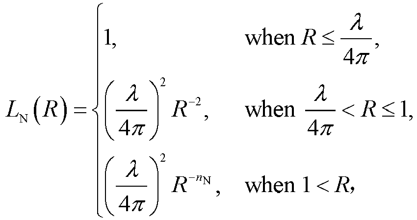
- the propagation model may be further defined as the two-ray ground-reflection model, wherein the path loss in the open space, LOS and NLOS indoor scenarios may be respectively predicted by the following equations.
- n L , and n N are the path loss exponent (PLE).
- PLE path loss exponent
- the wireless performance of a building can be defined by the coverage performance, the leakage performance, the capacity performance, or various other performance metrics.
- the wireless performance of a building is investigated by evaluating the impact of building structures on the signal to interference plus noise ratio (SINR), since the SINR constitutes a basis for further important metrics in wireless communications, such as coverage performance and capacity performance.
- SINR signal to interference plus noise ratio
- the wireless performance of a building is constrained by the building structure, which has no relationship with the deployment of antenna arrays and small cells.
- G I the interference power gain
- G P the intended power gain
- the interference power gain ( G I ) and the intended power gain ( G P ) of a building are metrics that can be used to understand a building's wireless performance.
- SINR signal to interference plus noise ratio
- the open space is a space which has no buildings or other surroundings. This means that no reflection, diffraction or transmission effects are introduced by a building's structure. Computationally, the size of the open space is limited to the same space as that of the building size. In the method described herein, we can assume that the differences between the evaluated SINR for the building and the SINR for the open space are as a result of the building structure.
- the interference gain G I and the power gain G P of buildings as the effective increase in the SINR by covering the building relative to the SINR in the open space scenario.
- G I is to capture the impact of blockage of interference signals by building structures.
- G P is to capture the impact of the building on the power of intended signals, where both the blockage and the waveguide effect are considered.
- ⁇ B P B I B + ⁇ 2 , where P B and I B respectively denote the overall power of intended signal and interference signal at the reference in the building.
- the signal received in the building could be separated into two parts. One part is the Line-of-Sight (LOS) signal, and the other part is the Non-Line-of-Sight (NLOS) signal. Then the overall power of the intended signal in the building could be separated into P L and P N , where P L and P N , respectively, denote received powers of intended signals from LOS and NLOS small cells/antenna elements.
- the overall interference signal in the building could be separated into I L and I N , respectively. I L and I N denote the LOS and the NLOS received powers of interference signals.
- G I and G P have different values.
- G I and G P have different values.
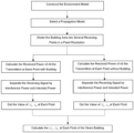
- a method for calculating G I and G P is schematically depicted in Figure 1 .
- the input information may include:
- Figure 2 is a flow diagram depicting an exemplary procedure for computing gains G I and G P .
- P os ⁇ 0 2 ⁇ ⁇ 0 R os P T L os R d R d ⁇
- I os ⁇ 0 2 ⁇ ⁇ R os + ⁇ P T L os R d R d ⁇ .
- a TM is the basic unit of a building area.
- the building structure can be separated into several TM.
- Each TM includes at least one of the following four areas, ⁇ PL , ⁇ PN , ⁇ IL , and ⁇ IN .
- ⁇ PL , ⁇ IL , ⁇ PN , and ⁇ IN denote the areas from where the transmitted signals are considered as LOS intended signals, LOS interference signals, NLOS intended signals, and NLOS interference signals by the reference UE, respectively.
- ⁇ PL , ⁇ IL , ⁇ PN , and ⁇ IN denote the areas from where the transmitted signals are considered as LOS intended signals, LOS interference signals, NLOS intended signals, and NLOS interference signals by the reference UE, respectively.
- TM we consider an area in the shape of a circular sector with an infinite radius. The reference UE is located in the vertex.
- a wall with a finite length, is modelled as a line segment located in the sector, and end points of the line segment are respectively located in both radiuses of the circular sector.
- the distance from the UE to the wall is denoted as D 0 .
- a polar coordinate system ( R , ⁇ ) is established by choosing the UE as the reference point and the perpendicular direction of the wall as the reference angle.
- ⁇ l and ⁇ r respectively denote angles of end points of the wall.
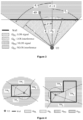
- Figure 3 depicts an example of the toy model, including schematic depictions of ⁇ PL , ⁇ PN , ⁇ IL , and ⁇ IN .
- one possible way of evaluating building wireless performance is to use ray tracing/ray launching based approaches.
- ray tracing/ray launching based approaches are both computational expensive, and dependent on exact Electro Magnetic properties of materials, and 3) network deployment relevant.
- Monte Carlo simulations are time consuming, inaccurate, and unavailable for fast optimization.
- an architect could use the method described herein for guidance regarding a building's wireless performance.
- the architect could use the method described herein to calculate the interference power gain ( G I ) and the intended power gain ( G P ) for their proposed building.
- An architect can then modify their proposed building structure so as to modify those values.
- a small interference power gain G I and a large intended power gain G P are generally associated with building's that exhibit good wireless performance.
- an architect may look to optimise a building for wireless performance by modifying the building structure so as to minimise G I and maximise G P .
- a user may evaluate the wireless performance of a building by defining wireless performance levels thresholds.
- the value of G increases when G I is decreased and / or G P is increased.
- the value, G may be compared with one or more performance level thresholds so as to evaluate the wireless performance of a building.
- the four thresholds may be termed: Th1, Th2, Th3 and Th4 where Th1>Th2>Th3>Th4.
- the thresholds may be predefined by analyzing a number of test buildings.
- the five wireless performance levels may be termed: Level A, Level B, Level C, Level D and Level E.
- the thresholds may be defined such that the test buildings are distributed across the performance levels according to a distribution rule, such as a normal distribution.
- the wireless performance of the building may be Level A
- the wireless performance of the building may be Level B
- the wireless performance of the building may be Level C
- the wireless performance of the building may be Level D
- the wireless performance of the building may be Level E.
- Level A may be considered to be the best performance level
- Level E may be considered to be the worst performance level. Such performance levels may be more easily understandable for the user.
- the methods described herein may be embodied in an apparatus for designing and evaluating buildings.
- a building model can be constructed in or imported to the apparatus.
- the building model can be analysed by the apparatus.
- the analysis can extract intermediate data to be used in the final calculation, such as a count of the number of walls, or rooms, the average wall thickness, or any other metrics.
- the apparatus may then request that the user inputs any further data or metrics that are required but are not derivable from the building model. For example, the user may be asked to specify the materials intended to be used for the construction of the building.
- the user may be asked to specify the type of building that is to be evaluated.
- the building may be a house, an office, a shopping mall, a train or bus station, a sports or music stadium, an airport, a tunnel, a ship, or any other type of building.
- this information may be available from the building model.
- the building model may then be evaluated by the apparatus.
- the apparatus may output metrics, such as the interference power gain and the intended power gain.
- the apparatus may output a performance level for the building model.
Landscapes
- Engineering & Computer Science (AREA)
- Computer Networks & Wireless Communication (AREA)
- Signal Processing (AREA)
- Physics & Mathematics (AREA)
- Electromagnetism (AREA)
- Quality & Reliability (AREA)
- Spectroscopy & Molecular Physics (AREA)
- Artificial Intelligence (AREA)
- Evolutionary Computation (AREA)
- Mobile Radio Communication Systems (AREA)
- Monitoring And Testing Of Transmission In General (AREA)
Description
- The present invention relates to wireless communications. More particularly, the present invention relates to a method for evaluating the wireless performance of a building so as to facilitate optimal construction or decoration of the building targeting a good performance of wireless networks within it.
- Wireless communication plays an important role in the smart building/city agenda. In a smart building, the internet of things (loTs) will be connected wirelessly to increase comfort of the indoor environment while reducing energy consumption. Hence, pursuing high capacity and reliable wireless communications indoors is fundamental and crucial.
- In wireless networks, interference is unwanted radio signal received at a receiver. The power of the intended signal and that of the interference signal at any given position indoors are determined by radio propagation that is affected by the layout of building structures. It is predictable that the building itself has a significant impact on wireless capacity.
- Therefore, different types of buildings have intrinsic wireless performances, independent of how densely small cells are deployed, or of the massive MIMO array antenna deployed. It is therefore reasonable to assume that the wireless network might not provide the desired indoor wireless performance in certain type of buildings as resources like frequency bands and power are limited. However, if a building is designed by taking its wireless performance into account at an early stage, then the desired wireless coverage and capacity would be considerably improved. This can be achieved, e.g., by providing building designers, both civil engineers and architects, with guidance on how to predict the wireless performance of buildings at the design stage. The wireless performance of the building itself has been ignored so far, which will be very important for future smart buildings in which appliances will be connected wirelessly. In the moment, the wireless metrics of building are not well designed considering layout of building structures. There is no publication focused on building wireless metric modelling or fast computation either.
- In the last century, the building design and construction community had been focused on improving safety, visual and thermal comfort, and indoor air quality. In the last decade, energy efficiency has become an important metric in building design, as set out in L. Atzori, et al., "The internet of things: a survey," Computer Networks, vol. 54, no. 15, pp. 2787-2805, 2010. For example, CIBSE, "TM54: evaluating operational energy performance of buildings at the design stage," CIBSE, 2013, sets out how the operational energy required for a building can be predicted, where covering lighting, heating, ventilation and cooling and provision of hot water are considered.
- Previous works have investigated the impact of building blockage on small cell networks. For example, T. Bai, et al., "Coverage and rate analysis for millimeter-wave cellular networks," IEEE Trans. Wireless Commun., vol. 4, no. 2, pp. 1100-1114, 2015, provided an analytic coverage rate by approximating the line of sight (LOS) region as a fixed LOS ball for a general LOS probability function. In M. K. Muller, et al., "Analyzing wireless indoor communications by blockage models," IEEE Access, vol. 5, pp. 2172-2186, 2017, four random wall generation methods to place blockage objects in an indoor scenario were proposed and analysed. Walls are either distributed randomly, semi-deterministically or heuristically. However, most of previous evaluation on the blockage effect is to assume buildings to form a process of random shapes, e.g., a Boolean scheme of rectangles, as in T. Bai, et al., "Analysis of blockage effects on urban cellular networks," IEEE Trans. Wireless Commun., vol. 13, no. 9, pp. 5070-5083, 2014, which are assumed to be homogenous. The homogenous blockage model is promising to provide insights on how to configure wireless network in a blockage scenario, but it is not suitable for evaluate specific inhomogeneous buildings in the real world.
- We describe herein the first work on evaluating building wireless performance based on given building layouts that will shed light on achievable wireless network performance in buildings.
- Rather than random blockages, ray-tracing/ray-launching technologies are employed to evaluate the performance of networks indoors for specific buildings, as set out in L. Azpilicueta, et al., "A hybrid ray launching-diffusion equation approach for propagation prediction in complex indoor environments," IEEE Ant. Wireless Prop. Lett., vol. 16, pp. 214-217, 2017. However, on one hand, results attained through this approach are always obtained for a specific deployment of network, and therefore are not general enough to evaluate buildings. We need to evaluate the building with tractable models, which are specified by a small set of parameters of wireless networks. On the other hand, the realization of ray-tracing/ray-launching is computational expensive when the environment is complicate, and therefore it is not applicable to evaluate buildings for all possible configurations of networks in a reasonable time.
-
WO 2015/097482 relates to a method of autonomous detection and positioning of indoor wireless network faults. - According to a first aspect there is provided a method for evaluating a building's wireless performance, characterized in that the method comprises: constructing an environment model, the environment model comprising a layout of the building, a power density of transmitters P T[W/m2], and a considered frequency band f c ; computing a signal to interference plus noise ratio (SINR) for the building in dependence on the environment model; computing a SINR for an open space in dependence on the environment model, the computing size for the open space being the same as the computing size of the building, and wherein the open space is an ideal space in absence of the building or other surroundings; comparing the SINR for the building with the SINR for the open space; and in dependence on the comparison, evaluating the building wireless performance by calculating an interference power gain and an intended power gain for the building.
- The interference power gain and the intended power gain for the building may be defined by the following equation,

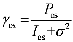
- The SINR for the open space may be computed by


- The overall power of the intended signal P B may comprise a LOS intended signal P L , and an NLOS intended signal P N, and the overall power of the interference signal I B may comprise a LOS interference signal I L , and an NLOS interference signal I N , the overall power of the intended signal P B and the overall power of the interference signal I B being defined by:


- The interference power gain (G I) and the intended power gain (G P) may be calculated by:


- The environment model may comprise a building model and a network model, the building model comprising the layout of the building, and the network model comprising positions of user equipment (UE), the power density of transmitters P T[W/m2], and the considered frequency band fc . and wherein the method may further comprise:
- 1) selecting a propagation model for calculating a path loss;
- 2) dividing the building into UE points in a fixed resolution;
- 3) calculating a receiving power from the transmitters in each UE point with the building;
- 4) calculating a receiving power from the transmitters in each UE point in the open space;
- 5) calculating the receiving interference signal and intended signal for each UE point within the building separately;
- 6) calculating the receiving interference signal and intended signal for each UE point in the open space separately;
- 7) Calculating the overall power of interference signal I B and the overall power of intended signal P B for each UE point in the building, and the overall power of interference signal I os and the overall power of intended signal P os for each UE point in the open space;
- 8) calculating the interference power gain (G I) and intended power gain (G P) for each UE point for the building.
- The propagation model may obey the law of conservation of energy and converge when the distance between a transmitter and a UE is infinitely large or infinitely small.
- The network model may be further restricted as an infinite number of transmitters, the transmitters being uniformly distributed in the environment, a reference UE taking use of all detectable power constrained by the sensitivity of its receiver, wherein detectable power is considered as the intended signal, and undetectable power is considered as the interference signal, wherein the detectable power may be defined as the power that is transmitted from transmitters that satisfy, P T L s(R) >P th and the undetectable power may be defined as the power that is transmitted from transmitters that satisfy PTLs (R) ≤P th, where s∈{os,B}, R denotes the distance from the reference UE to a reference transmitter, L s(R) denotes the path loss from the reference UE to the reference transmitter in the distance of R, Ω denote an arbitrary area, P th[W/m2] denotes a threshold constrained by the sensitivity of the UE receiver, for an arbitrary area Ω, the total transmit power from transmitter within Ω is P T A Ω, where A Ω is the area of Ω ; wherein the method may further comprise:
- calculating the intended signal, P os, by the following equation:

- calculating the interference signal, I os, by the following equation:

- calculating the intended signal P B by the following equation:

- calculating the interference signal I B by the following equation:

- where L os(R) denotes a pathloss from the reference UE to the reference transmitter in the distance of R in the open space, L B(R) denotes a pathloss from the reference UE to the referred transmit element in the distance of R in the building model.
- The values of P os and I os may be calculated by the following equations:


- The building model may be separated into a plurality of N TM Toy Models (TM), and P L, I L, P N, and I N may be calculated by the following equations:


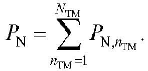

TM , IL,nTM , PN,nTM , IN,nTM respectively denote the LOS intended signal, LOS interference signal, NLOS intended signal and NLOS interference signal for one TM, wherein 1 ≤ nTM ≤ NTM . - Each TM may be separated into at most four areas, the said four areas being ΩPL, ΩIL, ΩPN, and ΩIN, and wherein P L,n
TM , I L,nTM , P N,nTM , and I N,nTM may be calculated by the following equations:


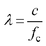
- The propagation model may be further defined as the two-ray ground-reflection model, wherein the path loss in the open space, LOS and NLOS indoor scenarios may be respectively predicted by the following equations.


- We describe herein an analytic framework to evaluate the wireless performance of buildings. On one hand, taking the open space scenario as a benchmark, metrics to measure wireless performances of buildings are well defined considering the impact of blockage, bounce reflections, and waveguide effect introduced by building structures.
- The advantages of the method described herein include:
- The proposed metrics capture the impact of a building on the wireless network within it. The impacts may include blockage, bounce reflection and waveguide effect.
- The proposed metrics are independent from specific deployment of small cells/distributed massive MIMO. Instead, they show a performance upper bound on networks indoors to reduce the set of parameters.
- Through the approach described herein, proposed metrics can be quickly and exactly computed to facilitate fast evaluation of buildings.
- The approach to compute metrics in closed forms described herein sheds light on optimization of building layout for architects.
- The present invention will now be described by way of example with reference to the accompanying drawings. In the drawings:
-
Figure 1 is a flow diagram depicting the computation procedure for gains G I and G P. - Figure 2 is a flow diagram depicting an exemplary procedure for computing gains G I and G P.
-
Figure 3 depicts an example of the toy model, including schematic depictions of ΩPL, ΩPN, ΩIL, and ΩIN. -
Figure 4 depicts example uses of a toy model to schematically represent: (a) a rectangular room, and (b) an L-shaped corner room. - The following description is presented to enable any person skilled in the art to make and use the invention, and is provided in the context of a particular application. Various modifications to the disclosed embodiments will be readily apparent to those skilled in the art.
- The general principles defined herein may be applied to other embodiments and applications without departing from the scope of the present invention as defined by the appended claims. Thus, the present invention as defined by the appended claims is not intended to be limited to the embodiments shown, but is to be accorded the widest scope consistent with the principles and features disclosed herein.
- Generally, the wireless performance of a building can be defined by the coverage performance, the leakage performance, the capacity performance, or various other performance metrics. In the method described herein, the wireless performance of a building is investigated by evaluating the impact of building structures on the signal to interference plus noise ratio (SINR), since the SINR constitutes a basis for further important metrics in wireless communications, such as coverage performance and capacity performance. The wireless performance of a building is constrained by the building structure, which has no relationship with the deployment of antenna arrays and small cells. In the method described herein, we derive values for the interference power gain (G I) and the intended power gain (G P) at a reference position of a building. The interference power gain (G I) and the intended power gain (G P) of a building are metrics that can be used to understand a building's wireless performance.
- Definition of Interference Gain G I and Power Gain G P.
- The impact of a building on its wireless network is evaluated by comparing the signal to interference plus noise ratio (SINR) indoors with that in the open space.
- The open space is a space which has no buildings or other surroundings. This means that no reflection, diffraction or transmission effects are introduced by a building's structure. Computationally, the size of the open space is limited to the same space as that of the building size. In the method described herein, we can assume that the differences between the evaluated SINR for the building and the SINR for the open space are as a result of the building structure.
- We propose herein an analytic framework to evaluate the wireless performance of a building. Taking the open space environment as a benchmark, metrics to measure wireless performances of a building are defined considering the impact of blockage, bounce reflections, and waveguide effect introduced by building structures. Through the approach, proposed metrics can be quickly and exactly computed.
- We investigate the impact of building structures on the SINR since it constitutes a basis for further important metrics in wireless communications, such as coverage and rate. We define the interference gain G I and the power gain G P of buildings as the effective increase in the SINR by covering the building relative to the SINR in the open space scenario. G I is to capture the impact of blockage of interference signals by building structures. G P is to capture the impact of the building on the power of intended signals, where both the blockage and the waveguide effect are considered.
- In the open space, the SINR is computed by γ os :

- Whereas with the impact of the building, the SINR in the building is computed by γ B :

- The signal received in the building could be separated into two parts. One part is the Line-of-Sight (LOS) signal, and the other part is the Non-Line-of-Sight (NLOS) signal. Then the overall power of the intended signal in the building could be separated into P L and P N , where P L and P N , respectively, denote received powers of intended signals from LOS and NLOS small cells/antenna elements. The overall interference signal in the building could be separated into I L and I N, respectively. I L and I N denote the LOS and the NLOS received powers of interference signals.
- That is:


- Therefore, we have the expression of the SINR in the building as:

- Combining (1) and (5), we obtain


- It is needed to emphasize that at different positions in the room, G I and G P have different values. To facilitate the comparison of rooms in terms of wireless performance, for each considered room, we compute the average G I and the average G P for a given room.
- Calculating the Interference Gain G I and Power Gain G P.
- A method for calculating G I and G P is schematically depicted in
Figure 1 . - As shown in
Figure 1 , the input information may include: - 1. The building layout, specifically the region inside the building is evaluated.
- 2. The position of one or more transmitters.
- 3. A path loss model, taking the transmit frequency fc into account.
- 4. The transmit power density of the transmitters (PT[W / m2]). and a threshold constrained by the sensitivity of the UE receiver (P th [W / m2]).
- Figure 2 is a flow diagram depicting an exemplary procedure for computing gains G I and G P.
- As shown in Figure 2, the values of G I and G P could be calculated by the following process:
- 1. Construct an environment model, which includes the building layout, the power density of transmitters P T[W/m2], and the considered frequency band fc .
- 2. Select a propagation model used to calculate the path gain of the transmitter, which could be a ray-tracing based model, a ray-launching based model, a multi-slope path loss model, etc.
- 3. Divide the building area into a finite number of the positions of the user equipment (UE) points in a fixed resolution.
- 4. Calculate the received power at each UE point from all the transmitters for the building and for the open space, separately.
- 5. Separate the receiving signal by interference power and intended power at each UE point in conditions of with building and open space, separately.
- 6. Calculating the overall power values of P os, I os, P B , and I B at each UE point.
- 7. Calculate the G I, G P at each UE point for the building.
- To get a closed form of G I, G P, we make the following 3 assumptions:
- 1. Assume that we have an infinite number of transmit elements, i.e., small cells or antenna elements, which are uniformly distributed in the environment. Infinite functions do not exist, therefore in order to simulate this assumption is it possible to model a large number of transmitters. The larger the number of transmitters modelled the closer the output is to the theoretical output of an infinite number of transmitters. That is, modelling a higher number of transmitters can increase the accuracy with which the performance of the building is evaluated. For an arbitrary area Ω, the total transmit power from transmit elements within Ω is P T A Ω, where A Ω is the area of Ω, and P T[W/m2]denotes the transmit power from a unit area.
- 2. The propagation model, which should obey the convergence rule when the distance from the antenna element to the UE is infinitely large and infinitely small.
- 3. Assume the reference UE can take use of all detectable power constrained by the sensitivity of its receiver in the networks. The detectable power is defined as the power that are transmitted from small cells/antenna elements that satisfies P T Ls (R)> P th, where s ∈{os,L,N}, R denotes the distance from the reference UE to the referred small cell/antenna element. L os(R), L L(R), and L N(R) denotes the path loss in the distance of R under open space, LOS and NLOS scenario.
- Under this assumption, the overall useful power transmitted in the building area could be calculated by the following equation:

- The overall interference power transmitted in the building area could be calculated by the following equation:

- The value of P os, I os in the open space could be calculated by the following equations:


- In general, computation of I L , P L , I N , and P N is not straightforward since the indoor scenarios are not homogeneous. To facilitate the derivation of interference and intended signal powers, we propose a toy model (TM).
- A TM is the basic unit of a building area. For any type of building structure, the building structure can be separated into several TM. Each TM includes at least one of the following four areas, ΩPL, ΩPN, ΩIL, and ΩIN. where ΩPL , ΩIL , ΩPN , and ΩIN denote the areas from where the transmitted signals are considered as LOS intended signals, LOS interference signals, NLOS intended signals, and NLOS interference signals by the reference UE, respectively. In the TM, we consider an area in the shape of a circular sector with an infinite radius. The reference UE is located in the vertex. A wall, with a finite length, is modelled as a line segment located in the sector, and end points of the line segment are respectively located in both radiuses of the circular sector. The distance from the UE to the wall is denoted as D 0 . A polar coordinate system (R,θ) is established by choosing the UE as the reference point and the perpendicular direction of the wall as the reference angle. θ l and θ r respectively denote angles of end points of the wall.
-
Figure 3 depicts an example of the toy model, including schematic depictions of ΩPL, ΩPN, ΩIL, and ΩIN. - It is observed that rooms with line segment shaped borders, can be considered as integration of several TMs.
Figure 4 depicts example uses of a toy model to schematically represent: (a) a rectangular room, and (b) an L-shaped corner room. In an instant direction, whether an area is LOS or NLOS is determined by the closest wall. If a room is integrated by N TM TMs, we have



- Therefore, as long as we have closed form expressions I L,n
TM , P L,nTM , I N,nTM , and P N,nTM , it is straightforward to compute I L , P L, I N, and P N by (13-16). - Considering Assumption 3, for arbitrary n TM we have



- We choose the two-ray ground-reflection model for an example, the path loss under open space, LOS and NLOS indoor scenarios are respectively predicted as:


- Combine the formula (11) (12) and (21), we can get the of expression of P os, I os.
- Combine the formula (13)(14)(17)(18) and (22), we can get the expression of I L, P L.
- Combine the formula (15)(16)(19)(20) and (23), we can get the expression of I N , P N.
- Then we can evaluate the building wireless performance by computing G I and G P.
- In some typical prior art systems, one possible way of evaluating building wireless performance is to use ray tracing/ray launching based approaches. Compared to the method described herein, ray tracing/ray launching based approaches are both computational expensive, and dependent on exact Electro Magnetic properties of materials, and 3) network deployment relevant.
- In other typical prior art systems, another possible way to compute wireless performance metrics is to use Monte Carlo simulations. Compared to the method described herein, Monte Carlo simulation based approaches are time consuming, inaccurate, and unavailable for fast optimization.
- During the design stages, an architect could use the method described herein for guidance regarding a building's wireless performance. By inputting a proposed building structure the architect could use the method described herein to calculate the interference power gain (G I) and the intended power gain (G P) for their proposed building. An architect can then modify their proposed building structure so as to modify those values. A small interference power gain G I and a large intended power gain G P are generally associated with building's that exhibit good wireless performance. Thus, an architect may look to optimise a building for wireless performance by modifying the building structure so as to minimise G I and maximise G P.
- In an example, a user may evaluate the wireless performance of a building by defining wireless performance levels thresholds. A new value, G, for comparison with the performance level thresholds may be defined by:

- In this example, the value of G increases when GI is decreased and/or GP is increased.
- In other examples, G may be defined by any equation in which the value of G increases when G I is decreased and/or G P is increased, such as:


- The value, G, may be compared with one or more performance level thresholds so as to evaluate the wireless performance of a building. For example, there may be five levels of wireless performance for a building defined by four thresholds. The four thresholds may be termed: Th1, Th2, Th3 and Th4 where Th1>Th2>Th3>Th4. The thresholds may be predefined by analyzing a number of test buildings. The five wireless performance levels may be termed: Level A, Level B, Level C, Level D and Level E. The thresholds may be defined such that the test buildings are distributed across the performance levels according to a distribution rule, such as a normal distribution. When G ≥ Th1, the wireless performance of the building may be Level A, when Th2 ≤ G < Th1, the wireless performance of the building may be Level B, when Th3 ≤ G < Th2, the wireless performance of the building may be Level C, when Th4 ≤ G < Th3, the wireless performance of the building may be Level D, when G < Th4, the wireless performance of the building may be Level E. In this example, Level A may be considered to be the best performance level and Level E may be considered to be the worst performance level. Such performance levels may be more easily understandable for the user.
- The methods described herein may be embodied in an apparatus for designing and evaluating buildings. In order to evaluate the wireless performance of the building, a building model can be constructed in or imported to the apparatus. The building model can be analysed by the apparatus. The analysis can extract intermediate data to be used in the final calculation, such as a count of the number of walls, or rooms, the average wall thickness, or any other metrics. The apparatus may then request that the user inputs any further data or metrics that are required but are not derivable from the building model. For example, the user may be asked to specify the materials intended to be used for the construction of the building. The user may be asked to specify the type of building that is to be evaluated. For example, the building may be a house, an office, a shopping mall, a train or bus station, a sports or music stadium, an airport, a tunnel, a ship, or any other type of building. In other examples, this information may be available from the building model. The building model may then be evaluated by the apparatus. The apparatus may output metrics, such as the interference power gain and the intended power gain. In another example, as described herein, the apparatus may output a performance level for the building model.
- The applicant hereby discloses in isolation each individual feature described herein and any combination of two or more such features, to the extent that such features or combinations are capable of being carried out based on the present specification as a whole in the light of the common general knowledge of a person skilled in the art, irrespective of whether such features or combinations of features solve any problems disclosed herein, and without limitation to the scope of the claims. The applicant indicates that aspects of the present invention may consist of any such individual feature or combination of features. In view of the foregoing description it will be evident to a person skilled in the art that various modifications may be made within the scope of the invention, which is defined by the appended claims.
Claims (14)
- A method for evaluating a building's wireless performance, the method comprising:constructing an environment model, the environment model comprising a layout of the building, a power density of transmitters P T[W/m2], and a considered frequency band fc ;computing a signal to interference plus noise ratio SINR for the building independence on the environment model;computing a SINR for an open space in dependence on the environment model, the computing size for the open space being the same as the computing size of the building, and wherein the open space is an ideal space in absence of the building or other surroundings;comparing the SINR for the building with the SINR for the open space; and in dependence on the comparison, evaluating the building wireless performance by calculating an interference power gain and an intended power gain for the building.
- The method as claimed in claim 1, wherein the interference power gain and the intended power gain at a reference position of the building are defined by the following equation,

- The method as claimed in claim 1 or claim 2, wherein the SINR for the open space is computed by


- The method as claimed in claim 3, wherein the overall power of the intended signal P B comprises a LOS intended signal P L, and an NLOS intended signal P N , and the overall power of the interference signal I B comprises a LOS interference signal I L, and an NLOS interference signal I N , the overall power of the intended signal P B and the overall power of the interference signal I B being defined by:


- The method as claimed in claim 4, wherein the interference power gain G I and the intended power gain G P are calculated by:


- The method as claimed in any of claims3 to 5, wherein the environment model comprises a building model and a network model, the building model comprising the layout of the building, and the network model comprising positions of UE, the power density of transmitters P T[W/m2], and the considered frequency band fc . and wherein the method further comprises:1) selecting a propagation model for calculating a path loss;2) dividing the building into one or more UE points in a fixed resolution;3) calculating a receiving power from the transmitters in each UE point with the building;4) calculating a receiving power from the transmitters in each UE point in the open space;5) calculating the receiving interference signal and intended signal for each UE point within the building separately;6) calculating the receiving interference signal and intended signal for each UE point in the open space separately;7) calculating the overall power of interference signal I B and the overall power of intended signal P B for each UE point in the building, and the overall power of interference signal I os and the overall power of intended signal P os for each UE point in the open space;8) calculating the interference power gain (G I) and intended power gain (G P) for each UE point for the building.
- The method as claimed in claim 6, wherein the propagation model obeys the convergence rule when the distance between a transmitter and a UE is infinitely large or infinitely small.
- The method as claimed in claim 6 or 7, wherein the network model is further restricted as an infinite number of transmitters, the transmitters being uniformly distributed in the environment, a reference UE taking use of all detectable power constrained by the sensitivity of its receiver, wherein detectable power is considered as the intended signal, and undetectable power is considered as the interference signal, wherein the detectable power is defined as the power that is transmitted from transmitters that satisfy, P T L s(R) >P th and the undetectable power is defined as the power that is transmitted from transmitters that satisfy P T L s(R)≤P th, where s∈{os,B}, R denotes the distance from the reference UE to a reference transmitter, Ls (R) denotes the pathloss from the reference UE to the reference transmitter in the distance of R, Ω denote an arbitrary area, P th[W/m2] denotes a threshold constrained by the sensitivity of the UE receiver, for an arbitrary area Ω, the total transmit power from transmitter within Ω is P T A Ω, where A Ω is the area of Ω; wherein the method further comprises:calculating the intended signal, P os, by the following equation:
 calculating the interference signal, I os, by the following equation:
 calculating the intended signal P B by the following equation:
 and calculating the interference signal I B by the following equation:
 where L os(R) denotes a pathloss from the reference UE to the reference transmitter in the distance of R in the open space, L B(R) denotes a pathloss from the reference UE to the referred transmit element in the distance of R in the building model.
 - The method as claimed in any of claims 6 to 8, wherein the values of P os and I os are calculated by the following equations:


- The method as claimed in any of claims 6 to 9, wherein the building model is separated into a plurality of N TM Toy Models TM, and wherein P L , I L , P N, and
I N are calculated by the following equations:


TM , I L,nTM , P N,nTM, and I N,nTM respectively denote the LOS intended signal, LOS interference signal, NLOS intended signal and NLOS interference signal for one TM , wherein 1 ≤ n TM ≤ N TM. - The method as claimed in claim 10, wherein each TM is separated into at most four areas, the said four areas being ΩPL, ΩIL, ΩPN, and ΩIN, and wherein P L,n
TM , I L,nTM, P N,nTM, and IN,nTM are calculated by the following equations:


- The method as claimed in any of claims 6 to 11, wherein the propagation model is further defined as the two-ray ground-reflection model, and wherein the path loss in the open space, LOS and NLOS indoor scenarios are respectively predicted by the following equations.



- The method as claimed in any preceding claim, wherein a wireless performance level for the building is determined in dependence on a function of the intended power gain and the interference power gain.
- The method as claimed in claim 13, wherein the function of the intended power gain and the interference power gain is compared to one or more predetermined thresholds so as to determine the wireless performance level for the building.
Applications Claiming Priority (2)
| Application Number | Priority Date | Filing Date | Title |
|---|---|---|---|
| GBGB1810995.9A GB201810995D0 (en) | 2018-07-04 | 2018-07-04 | Evaluating the wireless performance of a building |
| PCT/GB2019/051869 WO2020008181A1 (en) | 2018-07-04 | 2019-07-01 | Evaluating the wireless performance of a building |
Publications (3)
| Publication Number | Publication Date |
|---|---|
| EP3818742A1 EP3818742A1 (en) | 2021-05-12 |
| EP3818742B1 true EP3818742B1 (en) | 2023-08-30 |
| EP3818742C0 EP3818742C0 (en) | 2023-08-30 |
Family
ID=63143750
Family Applications (1)
| Application Number | Title | Priority Date | Filing Date |
|---|---|---|---|
| EP19736476.3A Active EP3818742B1 (en) | 2018-07-04 | 2019-07-01 | Evaluating the wireless performance of a building |
Country Status (5)
| Country | Link |
|---|---|
| US (1) | US11323891B2 (en) |
| EP (1) | EP3818742B1 (en) |
| CN (1) | CN112369060B (en) |
| GB (1) | GB201810995D0 (en) |
| WO (1) | WO2020008181A1 (en) |
Families Citing this family (2)
| Publication number | Priority date | Publication date | Assignee | Title |
|---|---|---|---|---|
| GB201810995D0 (en) | 2018-07-04 | 2018-08-15 | Ranplan Wireless Network Design Ltd | Evaluating the wireless performance of a building |
| CN115468604B (en) * | 2022-09-15 | 2025-03-25 | 广东电网有限责任公司 | Method, device and system for monitoring wiring status of PT protection device |
Family Cites Families (16)
| Publication number | Priority date | Publication date | Assignee | Title |
|---|---|---|---|---|
| US6446031B1 (en) | 1999-01-22 | 2002-09-03 | The University Of Akron | Cone mapping physical optics for design of indoor communication system |
| WO2001052581A1 (en) * | 2000-01-12 | 2001-07-19 | Ericsson Inc. | Indoor wireless communication system with cancellation of interference |
| US6625454B1 (en) * | 2000-08-04 | 2003-09-23 | Wireless Valley Communications, Inc. | Method and system for designing or deploying a communications network which considers frequency dependent effects |
| US7295960B2 (en) | 2003-01-22 | 2007-11-13 | Wireless Valley Communications, Inc. | System and method for automated placement or configuration of equipment for obtaining desired network performance objectives |
| US7203520B2 (en) * | 2003-09-30 | 2007-04-10 | Nortel Networks Limited | Beam wobbling for increased downlink coverage and capacity |
| JP2007251755A (en) * | 2006-03-17 | 2007-09-27 | Ntt Docomo Inc | Wireless communication system, base station, measuring apparatus, and wireless parameter control method |
| DE102007028066B3 (en) * | 2007-06-19 | 2009-02-12 | Infineon Technologies Ag | Method and apparatus for generating a transmission signal |
| CN103702338B (en) * | 2013-12-24 | 2017-04-12 | 英国Ranplan无线网络设计公司 | Method for rapidly establishing indoor wireless signal fingerprint database |
| CN103648113B (en) | 2013-12-24 | 2017-04-12 | 英国Ranplan无线网络设计公司 | Indoor wireless network fault autonomous detection and positioning method |
| CN103974285B (en) | 2014-04-15 | 2017-10-31 | 北京邮电大学 | Interference analysis method and system of a kind of cellular system to the single station |
| CN104363616B (en) | 2014-10-27 | 2018-07-03 | 英国Ranplan无线网络设计公司 | A kind of method of the indoor three dimensions field strength of outdoor to indoor propagation model prediction |
| WO2017039521A1 (en) | 2015-09-04 | 2017-03-09 | Telefonaktiebolaget Lm Ericsson (Publ) | Systems and methods for performing node deployment in an enclosure |
| EP3520459A1 (en) * | 2016-09-29 | 2019-08-07 | British Telecommunications Public Limited Company | Network range and connectivity improvenment |
| TWI624168B (en) | 2016-10-21 | 2018-05-11 | 元智大學 | An intelligent deployment cascade control device based on an fdd-ofdma indoor small cell in multi-user and interference environments |
| CN106792826B (en) * | 2016-12-30 | 2020-08-18 | 国家无线电监测中心检测中心 | Signal interference analysis method and device |
| GB201810995D0 (en) | 2018-07-04 | 2018-08-15 | Ranplan Wireless Network Design Ltd | Evaluating the wireless performance of a building |
-
2018
- 2018-07-04 GB GBGB1810995.9A patent/GB201810995D0/en not_active Ceased
-
2019
- 2019-07-01 EP EP19736476.3A patent/EP3818742B1/en active Active
- 2019-07-01 CN CN201980045021.6A patent/CN112369060B/en active Active
- 2019-07-01 US US17/255,609 patent/US11323891B2/en active Active
- 2019-07-01 WO PCT/GB2019/051869 patent/WO2020008181A1/en not_active Ceased
Also Published As
| Publication number | Publication date |
|---|---|
| CN112369060B (en) | 2024-06-07 |
| US11323891B2 (en) | 2022-05-03 |
| US20210266759A1 (en) | 2021-08-26 |
| CN112369060A (en) | 2021-02-12 |
| EP3818742A1 (en) | 2021-05-12 |
| EP3818742C0 (en) | 2023-08-30 |
| GB201810995D0 (en) | 2018-08-15 |
| WO2020008181A1 (en) | 2020-01-09 |
Similar Documents
| Publication | Publication Date | Title |
|---|---|---|
| Anjinappa et al. | Base station and passive reflectors placement for urban mmWave networks | |
| US10284316B2 (en) | Method for predicting indoor three-dimensional space signal field strength using an outdoor-to-indoor propagation model | |
| Bai et al. | Using random shape theory to model blockage in random cellular networks | |
| Zhang et al. | Wireless performance evaluation of building layouts: Closed-form computation of figures of merit | |
| Zhang et al. | Wireless energy efficiency evaluation for buildings under design based on analysis of interference gain | |
| Li et al. | Simulation and modeling of millimeter-wave channel at 60 GHz in indoor environment for 5G wireless communication system | |
| Li et al. | Millimeter-wave channel simulation and statistical channel model in the cross-corridor environment at 28 GHz for 5G wireless system | |
| Oehmann et al. | SINR model with best server association for high availability studies of wireless networks | |
| Zheng et al. | Exact line-of-sight probability for channel modeling in typical indoor environments | |
| US11323891B2 (en) | Evaluating the wireless performance of a building | |
| Chien et al. | Multi-Objective Optimization of 3-D Cell Deployment in Sustainable B5G/6G Networks: Balancing Performance and Sustainability | |
| Suto et al. | Propagation graph representation learning and its implementation in direct path representation | |
| Alwajeeh et al. | Efficient method for associating radio propagation models with spatial partitioning for smart city applications | |
| Shi et al. | Evaluation of building wireless performance for user equipment with aperture antenna | |
| Mirahmadi et al. | A building architecture model for predicting femtocell interference in next-generation networks | |
| Calin et al. | On the feasibility of outdoor-to-indoor LTE small cell deployments: Field trial experiments and performance prediction | |
| Baltzis | Distance distribution in convex n-gons: Mathematical framework and wireless networking applications | |
| Tu et al. | Performance comparison of MR-FDPF and ray launching in an indoor office scenario | |
| CN118802635B (en) | A method, apparatus and electronic device for determining community profile information | |
| Tran-Minh et al. | Application of raytracing technique for predicting average power distribution in indoor environment | |
| Yang et al. | Matlab simulink of COST231-WI Model | |
| Maviel et al. | A hybrid propagation model for large-scale variations caused by vehicular traffic in small cells | |
| Yu et al. | RNIndoor: A relay node deployment method for disconnected wireless sensor networks in indoor environments | |
| Palizban | Millimeter wave small cell network planning for outdoor line-of-sight coverage | |
| Zheng | Performance Analysis of Indoor Wireless Communications in Dense Cellular Networks |
Legal Events
| Date | Code | Title | Description |
|---|---|---|---|
| STAA | Information on the status of an ep patent application or granted ep patent |
Free format text: STATUS: UNKNOWN |
|
| STAA | Information on the status of an ep patent application or granted ep patent |
Free format text: STATUS: THE INTERNATIONAL PUBLICATION HAS BEEN MADE |
|
| PUAI | Public reference made under article 153(3) epc to a published international application that has entered the european phase |
Free format text: ORIGINAL CODE: 0009012 |
|
| STAA | Information on the status of an ep patent application or granted ep patent |
Free format text: STATUS: REQUEST FOR EXAMINATION WAS MADE |
|
| 17P | Request for examination filed |
Effective date: 20210111 |
|
| AK | Designated contracting states |
Kind code of ref document: A1 Designated state(s): AL AT BE BG CH CY CZ DE DK EE ES FI FR GB GR HR HU IE IS IT LI LT LU LV MC MK MT NL NO PL PT RO RS SE SI SK SM TR |
|
| DAV | Request for validation of the european patent (deleted) | ||
| DAX | Request for extension of the european patent (deleted) | ||
| GRAP | Despatch of communication of intention to grant a patent |
Free format text: ORIGINAL CODE: EPIDOSNIGR1 |
|
| STAA | Information on the status of an ep patent application or granted ep patent |
Free format text: STATUS: GRANT OF PATENT IS INTENDED |
|
| INTG | Intention to grant announced |
Effective date: 20230307 |
|
| GRAS | Grant fee paid |
Free format text: ORIGINAL CODE: EPIDOSNIGR3 |
|
| P01 | Opt-out of the competence of the unified patent court (upc) registered |
Effective date: 20230526 |
|
| GRAA | (expected) grant |
Free format text: ORIGINAL CODE: 0009210 |
|
| STAA | Information on the status of an ep patent application or granted ep patent |
Free format text: STATUS: THE PATENT HAS BEEN GRANTED |
|
| AK | Designated contracting states |
Kind code of ref document: B1 Designated state(s): AL AT BE BG CH CY CZ DE DK EE ES FI FR GB GR HR HU IE IS IT LI LT LU LV MC MK MT NL NO PL PT RO RS SE SI SK SM TR |
|
| REG | Reference to a national code |
Ref country code: GB Ref legal event code: FG4D |
|
| REG | Reference to a national code |
Ref country code: CH Ref legal event code: EP |
|
| REG | Reference to a national code |
Ref country code: DE Ref legal event code: R096 Ref document number: 602019036148 Country of ref document: DE |
|
| REG | Reference to a national code |
Ref country code: IE Ref legal event code: FG4D |
|
| U01 | Request for unitary effect filed |
Effective date: 20230929 |
|
| P04 | Withdrawal of opt-out of the competence of the unified patent court (upc) registered |
Effective date: 20231007 |
|
| U07 | Unitary effect registered |
Designated state(s): AT BE BG DE DK EE FI FR IT LT LU LV MT NL PT SE SI Effective date: 20231011 |
|
| PG25 | Lapsed in a contracting state [announced via postgrant information from national office to epo] |
Ref country code: GR Free format text: LAPSE BECAUSE OF FAILURE TO SUBMIT A TRANSLATION OF THE DESCRIPTION OR TO PAY THE FEE WITHIN THE PRESCRIBED TIME-LIMIT Effective date: 20231201 |
|
| PG25 | Lapsed in a contracting state [announced via postgrant information from national office to epo] |
Ref country code: IS Free format text: LAPSE BECAUSE OF FAILURE TO SUBMIT A TRANSLATION OF THE DESCRIPTION OR TO PAY THE FEE WITHIN THE PRESCRIBED TIME-LIMIT Effective date: 20231230 |
|
| PG25 | Lapsed in a contracting state [announced via postgrant information from national office to epo] |
Ref country code: RS Free format text: LAPSE BECAUSE OF FAILURE TO SUBMIT A TRANSLATION OF THE DESCRIPTION OR TO PAY THE FEE WITHIN THE PRESCRIBED TIME-LIMIT Effective date: 20230830 Ref country code: NO Free format text: LAPSE BECAUSE OF FAILURE TO SUBMIT A TRANSLATION OF THE DESCRIPTION OR TO PAY THE FEE WITHIN THE PRESCRIBED TIME-LIMIT Effective date: 20231130 Ref country code: IS Free format text: LAPSE BECAUSE OF FAILURE TO SUBMIT A TRANSLATION OF THE DESCRIPTION OR TO PAY THE FEE WITHIN THE PRESCRIBED TIME-LIMIT Effective date: 20231230 Ref country code: HR Free format text: LAPSE BECAUSE OF FAILURE TO SUBMIT A TRANSLATION OF THE DESCRIPTION OR TO PAY THE FEE WITHIN THE PRESCRIBED TIME-LIMIT Effective date: 20230830 Ref country code: GR Free format text: LAPSE BECAUSE OF FAILURE TO SUBMIT A TRANSLATION OF THE DESCRIPTION OR TO PAY THE FEE WITHIN THE PRESCRIBED TIME-LIMIT Effective date: 20231201 |
|
| PG25 | Lapsed in a contracting state [announced via postgrant information from national office to epo] |
Ref country code: PL Free format text: LAPSE BECAUSE OF FAILURE TO SUBMIT A TRANSLATION OF THE DESCRIPTION OR TO PAY THE FEE WITHIN THE PRESCRIBED TIME-LIMIT Effective date: 20230830 |
|
| PG25 | Lapsed in a contracting state [announced via postgrant information from national office to epo] |
Ref country code: ES Free format text: LAPSE BECAUSE OF FAILURE TO SUBMIT A TRANSLATION OF THE DESCRIPTION OR TO PAY THE FEE WITHIN THE PRESCRIBED TIME-LIMIT Effective date: 20230830 |
|
| PG25 | Lapsed in a contracting state [announced via postgrant information from national office to epo] |
Ref country code: SM Free format text: LAPSE BECAUSE OF FAILURE TO SUBMIT A TRANSLATION OF THE DESCRIPTION OR TO PAY THE FEE WITHIN THE PRESCRIBED TIME-LIMIT Effective date: 20230830 Ref country code: RO Free format text: LAPSE BECAUSE OF FAILURE TO SUBMIT A TRANSLATION OF THE DESCRIPTION OR TO PAY THE FEE WITHIN THE PRESCRIBED TIME-LIMIT Effective date: 20230830 Ref country code: ES Free format text: LAPSE BECAUSE OF FAILURE TO SUBMIT A TRANSLATION OF THE DESCRIPTION OR TO PAY THE FEE WITHIN THE PRESCRIBED TIME-LIMIT Effective date: 20230830 Ref country code: CZ Free format text: LAPSE BECAUSE OF FAILURE TO SUBMIT A TRANSLATION OF THE DESCRIPTION OR TO PAY THE FEE WITHIN THE PRESCRIBED TIME-LIMIT Effective date: 20230830 Ref country code: SK Free format text: LAPSE BECAUSE OF FAILURE TO SUBMIT A TRANSLATION OF THE DESCRIPTION OR TO PAY THE FEE WITHIN THE PRESCRIBED TIME-LIMIT Effective date: 20230830 |
|
| REG | Reference to a national code |
Ref country code: DE Ref legal event code: R097 Ref document number: 602019036148 Country of ref document: DE |
|
| PLBE | No opposition filed within time limit |
Free format text: ORIGINAL CODE: 0009261 |
|
| STAA | Information on the status of an ep patent application or granted ep patent |
Free format text: STATUS: NO OPPOSITION FILED WITHIN TIME LIMIT |
|
| 26N | No opposition filed |
Effective date: 20240603 |
|
| U20 | Renewal fee for the european patent with unitary effect paid |
Year of fee payment: 6 Effective date: 20240711 |
|
| P05 | Withdrawal of opt-out of the competence of the unified patent court (upc) changed |
Free format text: CASE NUMBER: APP_579006/2023 Effective date: 20231011 |
|
| PG25 | Lapsed in a contracting state [announced via postgrant information from national office to epo] |
Ref country code: MC Free format text: LAPSE BECAUSE OF FAILURE TO SUBMIT A TRANSLATION OF THE DESCRIPTION OR TO PAY THE FEE WITHIN THE PRESCRIBED TIME-LIMIT Effective date: 20230830 |
|
| REG | Reference to a national code |
Ref country code: CH Ref legal event code: PL |
|
| PG25 | Lapsed in a contracting state [announced via postgrant information from national office to epo] |
Ref country code: CH Free format text: LAPSE BECAUSE OF NON-PAYMENT OF DUE FEES Effective date: 20240731 |
|
| PGFP | Annual fee paid to national office [announced via postgrant information from national office to epo] |
Ref country code: GB Payment date: 20250619 Year of fee payment: 7 |
|
| U20 | Renewal fee for the european patent with unitary effect paid |
Year of fee payment: 7 Effective date: 20250619 |
|
| PG25 | Lapsed in a contracting state [announced via postgrant information from national office to epo] |
Ref country code: IE Free format text: LAPSE BECAUSE OF NON-PAYMENT OF DUE FEES Effective date: 20240701 |
|
| PG25 | Lapsed in a contracting state [announced via postgrant information from national office to epo] |
Ref country code: CY Free format text: LAPSE BECAUSE OF FAILURE TO SUBMIT A TRANSLATION OF THE DESCRIPTION OR TO PAY THE FEE WITHIN THE PRESCRIBED TIME-LIMIT; INVALID AB INITIO Effective date: 20190701 |
|
| PG25 | Lapsed in a contracting state [announced via postgrant information from national office to epo] |
Ref country code: HU Free format text: LAPSE BECAUSE OF FAILURE TO SUBMIT A TRANSLATION OF THE DESCRIPTION OR TO PAY THE FEE WITHIN THE PRESCRIBED TIME-LIMIT; INVALID AB INITIO Effective date: 20190701 |
|
| PG25 | Lapsed in a contracting state [announced via postgrant information from national office to epo] |
Ref country code: TR Free format text: LAPSE BECAUSE OF FAILURE TO SUBMIT A TRANSLATION OF THE DESCRIPTION OR TO PAY THE FEE WITHIN THE PRESCRIBED TIME-LIMIT Effective date: 20230830 |