EP3761261A1 - Combining anatomical image datasets into one combined image dataset - Google Patents
Combining anatomical image datasets into one combined image dataset Download PDFInfo
- Publication number
- EP3761261A1 EP3761261A1 EP19184384.6A EP19184384A EP3761261A1 EP 3761261 A1 EP3761261 A1 EP 3761261A1 EP 19184384 A EP19184384 A EP 19184384A EP 3761261 A1 EP3761261 A1 EP 3761261A1
- Authority
- EP
- European Patent Office
- Prior art keywords
- image dataset
- dataset
- anatomical
- datasets
- calibration image
- Prior art date
- Legal status (The legal status is an assumption and is not a legal conclusion. Google has not performed a legal analysis and makes no representation as to the accuracy of the status listed.)
- Granted
Links
Images



Classifications
-
- G—PHYSICS
- G06—COMPUTING OR CALCULATING; COUNTING
- G06T—IMAGE DATA PROCESSING OR GENERATION, IN GENERAL
- G06T3/00—Geometric image transformations in the plane of the image
- G06T3/40—Scaling of whole images or parts thereof, e.g. expanding or contracting
- G06T3/4038—Image mosaicing, e.g. composing plane images from plane sub-images
-
- G—PHYSICS
- G06—COMPUTING OR CALCULATING; COUNTING
- G06T—IMAGE DATA PROCESSING OR GENERATION, IN GENERAL
- G06T5/00—Image enhancement or restoration
- G06T5/40—Image enhancement or restoration using histogram techniques
Definitions
- the present invention concerns a method of combining at least two anatomical image datasets into one combined image dataset, a storage medium, and magnetic resonance apparatus.
- a table is driven along an axis which is the longitudinal axis of the scanner.
- anatomical dataset shows an interesting portion of the subject and may show functional or morphological or any other interesting information.
- An anatomical image dataset usually has a higher resolution than the calibration datasets.
- the image datasets After the acquisition of the raw data the image datasets have to be processed to generate images. In case of MRI the datasets must be Fourier-transformed.
- the images taken at different positions are combined to combined images to cover a greater volume of the subject in one image.
- the problem can arise that the signal intensities of the combined images do not fit.
- one or more parts of the combined image show a weak contrast or seem to be darker than other parts. These parts have their origin in the images used for producing the combined images and are caused by a different scaling of original images.
- the method comprises the step making said combined image dataset available in electronic form as a data file.
- the first calibration image dataset and the second calibration image dataset are calibration image datasets as described above. It may be any image dataset that can be used for calibration purposes. They only have to fulfill the requirement to have at least two slices.
- the calibration image datasets are multi-slice image datasets. Then each calibration image dataset consists of several two-dimensional images which are shifted in slice selection direction.
- the calibration image datasets are three-dimensional image datasets. Then the phase encoding steps in the slice selection direction create the slices of the image.
- the phase encoding direction and the slice selection direction may be distinguished only by definition because there are two phase encoding directions.
- the anatomical image datasets are multi-slice image datasets. In a second embodiment the anatomical image datasets are three-dimensional image datasets.
- the anatomical image datasets and the calibration image datasets have the same type of image, e.g. both are multi-slice image datasets.
- the calibration image datasets are shifted in one direction. That means that they show different examination volumes of the subject. This may be caused by a movement of the subject between the measurements of the calibration image datasets.
- Every slice of a calibration image dataset consists of a plurality of signal intensities, phase values, and so on. Therefore, a frequency distribution of any image parameter can be calculated for every slice.
- these frequency distributions can be compared.
- the comparison leads to a correction factor, which is caused by a difference between the frequency distributions. It can be used then to adapt the signal intensities of the calibration images.
- the correction factor may be used to adapt the signal intensities of the first anatomical image dataset and the second anatomical image dataset.
- the reason causing the different scaling is assumed to happen during the shift of the examined volume of the subject.
- the correction factor can be received from every pair of images and not only by the anatomical image datasets itself.
- a frequency distribution is calculated for a parameter of at least one slice of each calibration image dataset, and a correction factor for correcting signal intensities of at least one anatomical image dataset is calculated.
- a corrected and therefore normalized second anatomical image dataset can be created.
- This normalization occurs with regard to the first anatomical image dataset. Since there is no absolute signal intensity to that a normalization could take place the first calibration image dataset and first anatomical image dataset is taken respectively. Of course, it is the calibration image datasets where the frequency distributions are calculated from, but in the same way the anatomical image datasets are respected.
- the number of correction factors to be calculated equals to the number of anatomical image datasets minus 1 assumed there is one anatomical image dataset per table position during examination.
- the number of correction factors to be calculated equals to the number of table positions during examination minus 1.
- a rule can be set up to choose one of the calibration image datasets being the first calibration image dataset. It may be the first one that is acquired or may be one in the center or may be chosen by a user. Moreover, it could be randomly chosen. Finally, one of the calibration image datasets has to be the first image dataset. The further calibration image datasets are normalized directly or indirectly to the first calibration image dataset.
- the anatomical image datasets are magnetic resonance image datasets.
- the calibration image datasets may be magnetic resonance image datasets.
- a histogram is used as frequency distribution. Moreover, the signal intensities of at least one slice are used to create the histogram of each calibration image dataset.
- the histograms of the calibration image datasets have similar profiles that mainly differ in a possible shift of the profiles. This shift is caused by the different scaling of the underlying images.
- a correction factor to correct the scaling can be directly derived from the histograms.
- the first calibration image dataset and the second calibration image dataset are image datasets for surface coil intensity correction.
- parallel imaging coil arrays of surface coils are used to acquire data.
- the coils can collect the data parallel at the same time.
- the surface coils can cover overlapping volumes and produce a higher SNR than larger, more distant coils.
- the signal acquired with a surface coil is not uniform.
- the signal has to be corrected for a first time to compensate the so called surface coil flare. This has to be done if a coil array is used, independent of the acquisition of second calibration image datasets or anatomical image datasets. It has to be done even if there is only one anatomical image dataset.
- the calculated correction factor for a table position may be applied to several anatomical images of that position, e.g. to a T1-map dataset and a FLASH image dataset and a turbo spin echo (TSE) image dataset.
- TSE turbo spin echo
- an anatomical image dataset is assigned to one calibration image dataset.
- the assignment is achieved by the position of the patient table which has to be the same. If the patient table is moved to a new position, also at the beginning, calibration measurements are executed and the desired calibration image dataset is acquired. Then one or more anatomical image datasets are acquired. As long as no action is taken that requires a new calibration the anatomical image or images are assigned to the current calibration image dataset.
- the first the anatomical image datasets is assigned to a correction factor being 1.
- the first calibration image dataset is taken as the image dataset the signal intensities of the further image datasets are normalized to.
- the signal intensities of the calibration image dataset and the anatomical image dataset are assumed to be correlated. Then the signal intensities of the first anatomical image dataset may remain unchanged which corresponds to a correction factor of 1.
- At least three anatomical image datasets and respective calibration image datasets are provided.
- the described normalization of signal intensities can be carried out for more than two calibration image datasets and anatomical image datasets.
- one of the three or more calibration image datasets has to be chosen to be the first calibration image dataset.
- the second calibration image dataset must be adjacent to the first calibration image dataset.
- the second calibration image dataset and the third calibration image dataset may be used to generate a correction factor for the third anatomical image dataset.
- the first calibration image dataset and the third calibration image dataset are used to calculate a correction factor for the third anatomical image dataset.
- the adjacent calibration image dataset is the second calibration image dataset and a correction factor cf1-2 for the second anatomical image dataset can be calculated using the first calibration image dataset and the second calibration image dataset.
- the third calibration image dataset is the next following the second calibration image dataset in line.
- a second correction factor cf2-3 is generated using the second calibration image dataset and the third calibration image dataset.
- the correction factor cf1-2 and the second correction factor cf2-3 have to be multiplied.
- the calculation of the correction factor is executed using one slice of each calibration image dataset.
- the neighboring slices or overlapping slices are taken.
- the slices are neighboring with regard to the position in the examined subject.
- the signal intensity distribution should be the same or nearly the same. Using a frequency distribution one can avoid errors due to changing extreme values.
- additional slices are used for the calculation of the histograms until a predefined condition is fulfilled. For example, a given number of signal intensity values has to be existent. Then starting with the neighboring slices adjacent slices of the calibration image dataset are taken to calculate the frequency distribution of a calibration image dataset.
- the same number of slices is used for generating the frequency distributions.
- three slices are used for the first calibration image dataset as well as three slices for the second calibration image dataset.
- the sequence used to acquire the calibration image datasets may be any sequence, but it is preferred to use a gradient echo sequence, e.g. a FLASH sequence.
- the sequence used to acquire the anatomical images is not limited to any special sequence.
- the neighboring slices used for normalization should have the same resolution, e.g. cover the same volume and have the same number of data points, which means the covered side lengths being equal. This avoids additional steps in the normalization process.
- the anatomical image datasets and/or calibration image datasets do not necessarily cover identically large volumes. Nevertheless, it is preferred that the first calibration image dataset has the same resolution like the second calibration image dataset and like the third calibration image dataset and so on. In case of a multi-slice calibration image dataset the first calibration image dataset may have six slices, the second one seven slices and the third one again six slices. But if they have an equal resolution in read and phase direction and slices having equal thickness the neighboring slices have the same resolution.
- the first anatomical image dataset has the same resolution like the first anatomical calibration image dataset and like the second anatomical image dataset and so on.
- the anatomical image datasets and the calibration image datasets may have the same resolution.
- the anatomical image datasets have a higher resolution in at least one direction.
- the calibration image datasets have a lower resolution than the anatomical image datasets.
- volume elements also called voxels, lying over a threshold are considered. Then the noise signal is respected neither calculating the correction factor nor being adjusted.
- the slices used for the calculation of a correction factor are adjacent slices of two neighboring calibration image datasets. Within these slices there should be no or not a big difference between the signal intensities as mentioned above.
- the table supporting the subject has had different positions when the calibration image datasets for normalizing the signal intensities have been acquired.
- the different examination volumes could exist the table having the same position. Then it was easier if one would acquire one image dataset, either calibration image dataset or anatomical image dataset, covering the whole volume and use it for normalization purposes.
- the calibration image datasets and/or anatomical image datasets cover more than 75 % of the homogeneous volume, at least in slice selection direction, of a magnetic resonance apparatus the image datasets being acquired with.
- the examination volume of the subject to be examined is at least in one direction larger than the homogeneous volume of the scanner. Then several scans at different table positions have to be acquired.
- the calibration image datasets and/or anatomical image datasets have been acquired using a different subset of a receive coil array.
- the first anatomical image dataset and the first calibration image dataset have been acquired with a first subset of the receive coil array
- the second anatomical image dataset and the second calibration image dataset have been acquired with a second subset of the receive coil array, and so forth.
- a magnetic resonance apparatus comprising:
- a non-transitory computer-readable data storage medium encoded with programming instructions is disclosed, said storage medium being loaded into a computer system of a magnetic resonance (MR) apparatus that comprises an MR data acquisition scanner having a radio-frequency (RF) transmitter, an RF receiver, a gradient coil arrangement, and a memory, said programming instructions causing said computer system to carry out the method described above.
- MR magnetic resonance
- RF radio-frequency
- FIG. 1 shows a magnetic resonance apparatus 1.
- the magnetic resonance apparatus 1 has a scanner 2.
- a transmit coil arrangement 3 is part of the scanner 2.
- the transmit coil arrangement 3 is usually designed as a body coil, and thus consists of a single coil.
- the magnetic resonance apparatus 1 has a receive coil arrangement 4.
- the receive coil arrangement 4 is designed as a coil array having coils 5, 6, 7 and 8.
- the receive coil arrangement 4 usually is laid on a movable patient table 9 and is positioned at least partly within the homogeneous area 10 of the scanner 2.
- the homogeneous area 10 is marked with dashed lines.
- the length of a spine is longer than the length of the homogeneous area 10.
- the acquisition has to be split into several measurements or images, each of them showing a part of the spine which is positioned in the homogeneous area 10.
- the center 11 of the homogeneous area 10 is marked by a dash.
- a control computer 12 controls the operation of the magnetic resonance apparatus 1.
- the magnetic resonance apparatus 1 also has a non-transitory data storage medium 13 as part of the control computer 12 or independent thereof, on which computer code for carrying out magnetic resonance measurements is stored.
- the coil array 4 is used only to read out the measurement signal which can be an echo signal.
- the coils 5, 6, 7 and 8 of the coil array 4 read out the measurement signal at the same time.
- Fig. 2 shows an exemplary positioning of calibration image datasets 14, 15 and 16 and anatomical image datasets 17, 18 and 19.
- the covered volumes for the calibration image dataset 14 and the anatomical image dataset 17 are preferably identical. Both cover the head 20 and the upper region of the spine 21. They cover the homogeneous area 10 completely to keep the measurement time as short as possible.
- calibration image dataset 15 and the anatomical image dataset 18 cover the identical volume, here the center of spine 21. This also holds for calibration image dataset 16 and the anatomical image dataset 19 which cover the lower end of spine 21 of the subject 22 to be examined.
- the calibration image datasets show different volumes of subject 22, but have been acquired in the same homogeneous area 10.
- table 10 has been moved after the acquisition of calibration image dataset 14 and anatomical image dataset 17 to measure calibration image dataset 15 and anatomical image dataset 18. Then it has been moved again to acquire calibration image dataset 16 and anatomical image dataset 19.
- Fig. 2 also shows a possible arrangement of the axis.
- the readout axis kx may be arranged upwards, the slice selection axis kz parallel to the longitudinal axis of scanner 2 and the phase encoding axis points into the sheet.
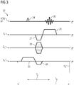
- Fig. 3 shows an exemplary sequence diagram 23 of a FLASH sequence.
- Axis RF shows the RF pulses and acquisition windows, axis G r the gradients in read direction, axis G pe the gradients in phase encoding direction and axis G s the gradients in slice selection direction. They correlate to the axis kx, ky and kz shown in Fig. 2 in the known manner.
- Excitation pulse 24 is the only RF pulse applied in the shown sequence diagram 23.
- Slice selection gradient 25 is applied at the same time to select a defined slice in subject 22. It is known to use an additional slice rephasing gradient 26 to compensate the dephasing fraction of the slice selection gradient 25.
- a dephasing gradient 27 in readout direction may be applied along with the slice rephrasing gradient 26 to get a minimal echo time T E . Also the phase encoding gradient 28 may be applied at the same time.
- a readout gradient 29 is applied after the dephasing gradient 27. This generates a gradient echo 30, which is acquired.
- All steps beginning at one excitation pulse, here RF pulse 24, to the next excitation pulse are part of an excitation cycle 31.
- the length of an excitation cycle is the repetition time T R .
- the excitation cycle is repeated n pe times, one repetition for one k-line of k-space which has to be acquired parallel by the coils 5, 6, 7 and 8. Due to the usage of coil array 4 the number of excitation cycles is reduced compared to the resolution of the image datasets 14, 15 and 16, because additional k-lines are generated to improve the resolution.
- Fig. 3 shows an acquisition scheme for a multi-slice calibration image dataset.
- the slice selection gradient 25 would be stepped through like the phase encoding gradient 28. Additionally, its strength would be chosen so that the complete volume was excited in every acquisition and not only a slice.
- the FLASH sequence diagram 23 is an exemplary sequence diagram for the acquisition of a calibration image dataset. Of course, other sequences could be used as well.
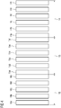
- Fig. 4 shows the three calibration image datasets 14, 15 and 16 being multi-slice image datasets.
- Calibration image dataset 14 has slices 14a, 14b, 14c, 14d, 14e and 14f.
- Calibration image dataset 15 has slices 15a, 15b, 15c, 15d, 15e and 15f.
- Calibration image dataset 16 has one slice less and therefore slices 16a, 16b, 16c, 16d, and 16e. Nevertheless, slices 14a, 14b, 14c, 14d, 14e, 14f, 15a, 15b, 15c, 15d, 15e, 15f, 16a, 16b, 16c, 16d, and 16e have the same resolution.
- May calibration image dataset 14 be chosen as first calibration image dataset and calibration image dataset 15 as second calibration image dataset.
- this neighboring calibration image dataset has to be the second calibration image dataset 15.
- the first calibration image dataset 14 and the second calibration image dataset 15 have neighboring slices 14a and 15f.
- slices 14a and 15f may overlap slightly.
- slices 14a and 15f could overlap completely, too. This is usually not made to save measurement time.
- a histogram 32 is calculated which is shown in Fig. 5 .
- the bins 33 to separate the signal intensities are preferably set before.
- Curve 34 of histogram 32 has an appearance that could be as shown in Fig. 5 .
- Axis 35 shows the bins 33 of the signal intensities and axis 36 the number of signal intensities within the bin.
- Fig. 6 shows a histogram 37 generated from the signal intensity values of slice 15f.
- the bins 33 are identically chosen.
- Curve 38 of histogram 37 is shifted in the direction of axis 35 compared to curve 34. This shift should not be there because slices 14a and 15f show neighboring or slightly overlapping regions of subject 22. Hence a wrong scaling is assumed to be the reason for the shift.
- cf1-2 a correction factor which may be called cf1-2.
- This correction factor cf1-2 can be derived from histograms 32 and 37 as follows: One extreme value could be chosen in the first histogram 32 and the second histogram 37, e.g the first maximum.
- the correction factor cf1-2 is received by dividing the number of the second histogram 37, here six, by the number of the first histogram, here three. Hence the correction factor cf1-2 was 2.
- correction factor cf1-2 one can step through a number of correction factors, apply on the signal intensities of the second calibration image dataset 15 and calculate a respective histogram 37 for every correction factor. Then the difference of histograms 32 and 37 may be computed. The correction factor producing the least difference is then taken as correction factor cf1-2.
- Bins 33 are identically chosen and therefore have a certain width which represents relative signal intensity values.
- the correction factor cf1-2 is derived from two calibration image datasets 14 and 15 but will be applied on the anatomical image dataset 18.
- a correction factor cf2-3 can be derived from slices 15a and 16e which are also neighboring slices of neighboring calibration image datasets 15 and 16.
- anatomical image dataset 19 has to be multiplied with both correction factors cf1-2 and cf2-3 to be normalized to anatomical image dataset 17, because correction factor cf2-3 only includes the difference to anatomical image 18.
- a correction factor cf1-3 could be calculated by using a second image calibration dataset 15' the signal intensity values already have been multiplied with the correction factor cf1-2.
- correction factor cf1-2 that normalizes slice 15f to slice 14a is used to normalize the signal intensity values of the second anatomical image 18 to those of the first anatomical image 17 and the product of the correction factors cf1-2 and cf2-3 to normalize the signal intensity values of the third anatomical image 19 to those of the first anatomical image 17.
- Fig. 7 shows a procedure diagram of generating a combined image dataset.
- table 10 is driven to the desired examination position.
- a calibration image dataset 17 for surface coil intensity correction is executed, e.g. in step S2 .
- additional experiments can be done in step S3 like the acquisition of the raw data of at least one anatomical image dataset 14.
- step S4 it is decided if more positions have to be examined. If so, steps S1 to S3 are repeated. If not, the raw data of the anatomical image datasets can be processed to image datasets in step S5 e.g. by carrying out a Fourier transform.
- step S6 the anatomical image datasets 17 to 19 are normalized by normalizing neighboring slices of the respective calibration image datasets 14 to 16 as described above. This step is described with more detail in Fig. 8 .
- the normalized anatomical images 17 to 19 are then combined to a combined image in step S7.
- Fig. 8 shows a procedure diagram of normalizing images using calibration image datasets.
- one of the calibration image datasets 14 to 16 is chosen to be the first calibration image dataset.
- one of the anatomical image datasets could be chosen or one of the positions of table 10. Then the datasets belonging to the same position of table 10 are also "first" ones. That means if calibration image dataset 14 is the first calibration image dataset, automatically anatomical image dataset 17 is the first anatomical image dataset.
- step S9 the second calibration image dataset and anatomical image dataset are selected.
- the only condition to be fulfilled is the second calibration image dataset being adjacent to the first calibration image dataset. Then automatically two adjacent slices exist.
- only calibration image dataset 15 can be taken as second calibration image dataset because it is the only neighbor of the first calibration image dataset 14.
- anatomical image dataset 18 is automatically the second anatomical image dataset.
- a histogram of slice 14a is generated.
- Slice 14a is that one of all slices of the first calibration image dataset 14 which is adjacent to the second calibration image dataset 15. For the same reason in step 11 a histogram 38 is generated for slice 15f.
- the curves 34 and 38 of histograms 32 and 37 are compared in step S12 to calculate correction factor cf1-2.
- step S13 the signal intensities of the second anatomical image 15 are normalized to the signal intensities of the first anatomical image 14 by multiplying the signal intensity values of each voxel with the correction factor cf1-2.
- step S14 it is decided if additional images have to be normalized. Then steps 8 to 13 are repeated with different pairs of calibration image datasets and anatomical image datasets.
- the signal intensities of the further anatomical image datasets are normalized to the first anatomical image dataset 17.
- Fig. 9 shows a schematic normalization for a first anatomical image dataset 39, a second anatomical image dataset 40 and a third anatomical image dataset 41.
- First anatomical image dataset 39 shows an upper part 42 of spine 21, second anatomical image dataset 40 the central part 43 and third anatomical dataset 41 a lower part 44 of spine 21.
- anatomical image datasets 39, 40 and 41 can be combined to a combined image dataset 45 having normalized signal intensities without intensity steps crossing the image borders of image datasets 39, 40 and 41.
Landscapes
- Physics & Mathematics (AREA)
- General Physics & Mathematics (AREA)
- Engineering & Computer Science (AREA)
- Theoretical Computer Science (AREA)
- Magnetic Resonance Imaging Apparatus (AREA)
Abstract
Description
- The present invention concerns a method of combining at least two anatomical image datasets into one combined image dataset, a storage medium, and magnetic resonance apparatus.
- To generate images of larger volumes different ways of acquiring data are known in medical imaging. Using a CT apparatus, the subject is positioned in a scanner which usually covers only a part of the subject. A typical MR apparatus is longer, but the homogeneous area is also limited to a small volume compared to the length of the MR apparatus.
- Therefore, to cover the whole body or at least a larger volume than the covered or homogeneous volume it is known to drive the subject through the scanner. To do so, a first part of the subject is examined, then it is positioned again so that a second part is covered and can be examined and so on until the last part has been examined.
- To change the position of the subject usually a table is driven along an axis which is the longitudinal axis of the scanner.
- In MRI several adjustments have to be done after the movement of the subject. First the resonance frequency has to be determined. Second the volume has to be shimmed. Third, if a coil array is used for the data acquisition, an image dataset for a surface coil intensity correction has to be acquired. Further adjustments may be carried out additionally. For all adjustments, calibration datasets are acquired, respectively.
- After the positioning of the subject and the adjustments where necessary one or more anatomical datasets can be measured. An anatomical dataset shows an interesting portion of the subject and may show functional or morphological or any other interesting information. An anatomical image dataset usually has a higher resolution than the calibration datasets.
- After the acquisition of the raw data the image datasets have to be processed to generate images. In case of MRI the datasets must be Fourier-transformed.
- Then the images taken at different positions are combined to combined images to cover a greater volume of the subject in one image. There the problem can arise that the signal intensities of the combined images do not fit. Then one or more parts of the combined image show a weak contrast or seem to be darker than other parts. These parts have their origin in the images used for producing the combined images and are caused by a different scaling of original images.
- Therefore, there is a need for a method of generating a combined image dataset the combined image dataset having reduced scaling problems.
- These needs are satisfied in a method according to the invention a method of combining at least two anatomical image datasets into one combined image dataset having the steps:
- a) providing a first calibration image dataset of a first examination volume of the subject having at least two slices,
- b) providing the first anatomical image dataset of the first examination volume of the subject,
- c) providing a second calibration image dataset of a second examination volume of the subject having at least two slices,
- d) providing the second anatomical image dataset of the second examination volume of the subject,
- e) wherein the calibration image datasets are shifted one against each other in one imaging direction, characterized in that
- f) a frequency distribution is calculated for a parameter of at least one slice of each calibration image dataset, and at least one correction factor for correcting signal intensities of at least one anatomical image dataset is calculated using the frequency distributions,
- g) generating a corrected second anatomical image dataset by adjusting the signal intensities of at least a region of the second anatomical image dataset using the correction factor, and
- h) combining the first anatomical dataset and the corrected second anatomical image dataset to a combined image dataset.
- Preferably, the method comprises the step making said combined image dataset available in electronic form as a data file.
- The first calibration image dataset and the second calibration image dataset are calibration image datasets as described above. It may be any image dataset that can be used for calibration purposes. They only have to fulfill the requirement to have at least two slices.
- In a first embodiment the calibration image datasets are multi-slice image datasets. Then each calibration image dataset consists of several two-dimensional images which are shifted in slice selection direction.
- In a second embodiment the calibration image datasets are three-dimensional image datasets. Then the phase encoding steps in the slice selection direction create the slices of the image. In this embodiment the phase encoding direction and the slice selection direction may be distinguished only by definition because there are two phase encoding directions.
- In a first embodiment the anatomical image datasets are multi-slice image datasets. In a second embodiment the anatomical image datasets are three-dimensional image datasets.
- Preferably the anatomical image datasets and the calibration image datasets have the same type of image, e.g. both are multi-slice image datasets.
- The calibration image datasets are shifted in one direction. That means that they show different examination volumes of the subject. This may be caused by a movement of the subject between the measurements of the calibration image datasets.
- Every slice of a calibration image dataset consists of a plurality of signal intensities, phase values, and so on. Therefore, a frequency distribution of any image parameter can be calculated for every slice.
- If one calculates at least one frequency distribution for each calibration image dataset, these frequency distributions can be compared. The comparison leads to a correction factor, which is caused by a difference between the frequency distributions. It can be used then to adapt the signal intensities of the calibration images.
- Moreover, and this is the core of the invention, the correction factor may be used to adapt the signal intensities of the first anatomical image dataset and the second anatomical image dataset. The reason causing the different scaling is assumed to happen during the shift of the examined volume of the subject. Hence the correction factor can be received from every pair of images and not only by the anatomical image datasets itself.
- A frequency distribution is calculated for a parameter of at least one slice of each calibration image dataset, and a correction factor for correcting signal intensities of at least one anatomical image dataset is calculated.
- Using the correction factor a corrected and therefore normalized second anatomical image dataset can be created. This normalization occurs with regard to the first anatomical image dataset. Since there is no absolute signal intensity to that a normalization could take place the first calibration image dataset and first anatomical image dataset is taken respectively. Of course, it is the calibration image datasets where the frequency distributions are calculated from, but in the same way the anatomical image datasets are respected.
- Preferably, the number of correction factors to be calculated equals to the number of anatomical image datasets minus 1 assumed there is one anatomical image dataset per table position during examination. In other words, the number of correction factors to be calculated equals to the number of table positions during examination minus 1.
- It has to be noted that a rule can be set up to choose one of the calibration image datasets being the first calibration image dataset. It may be the first one that is acquired or may be one in the center or may be chosen by a user. Moreover, it could be randomly chosen. Finally, one of the calibration image datasets has to be the first image dataset. The further calibration image datasets are normalized directly or indirectly to the first calibration image dataset.
- Preferably, the anatomical image datasets are magnetic resonance image datasets. Moreover, the calibration image datasets may be magnetic resonance image datasets.
- Advantageously a histogram is used as frequency distribution. Moreover, the signal intensities of at least one slice are used to create the histogram of each calibration image dataset. The histograms of the calibration image datasets have similar profiles that mainly differ in a possible shift of the profiles. This shift is caused by the different scaling of the underlying images. A correction factor to correct the scaling can be directly derived from the histograms.
- Preferably the first calibration image dataset and the second calibration image dataset are image datasets for surface coil intensity correction. In parallel imaging coil arrays of surface coils are used to acquire data. Using a coil array the coils can collect the data parallel at the same time. The surface coils can cover overlapping volumes and produce a higher SNR than larger, more distant coils. But the signal acquired with a surface coil is not uniform. Hence the signal has to be corrected for a first time to compensate the so called surface coil flare. This has to be done if a coil array is used, independent of the acquisition of second calibration image datasets or anatomical image datasets. It has to be done even if there is only one anatomical image dataset.
- If a coil array is used that covers a larger volume than the isotropic volume inside the MR scanner the patient table is moved and the same experiments are executed several times. Then also the calibration measurements are made several times.
- It has to be noted that several different calibration image datasets and anatomical image datasets may be acquired for every position of the table. Only one of the calibration image datasets is chosen, for example the above mentioned image dataset for surface coil intensity correction. The calculated correction factor for a table position may be applied to several anatomical images of that position, e.g. to a T1-map dataset and a FLASH image dataset and a turbo spin echo (TSE) image dataset.
- Advantageously an anatomical image dataset is assigned to one calibration image dataset. The assignment is achieved by the position of the patient table which has to be the same. If the patient table is moved to a new position, also at the beginning, calibration measurements are executed and the desired calibration image dataset is acquired. Then one or more anatomical image datasets are acquired. As long as no action is taken that requires a new calibration the anatomical image or images are assigned to the current calibration image dataset.
- Preferably the first the anatomical image datasets is assigned to a correction factor being 1. With other words the first calibration image dataset is taken as the image dataset the signal intensities of the further image datasets are normalized to. The signal intensities of the calibration image dataset and the anatomical image dataset are assumed to be correlated. Then the signal intensities of the first anatomical image dataset may remain unchanged which corresponds to a correction factor of 1.
- Advantageously at least three anatomical image datasets and respective calibration image datasets are provided. The described normalization of signal intensities can be carried out for more than two calibration image datasets and anatomical image datasets. In this case one of the three or more calibration image datasets has to be chosen to be the first calibration image dataset. The second calibration image dataset must be adjacent to the first calibration image dataset.
- If the third calibration image dataset is adjacent to the second calibration image dataset, the second calibration image dataset and the third calibration image dataset may be used to generate a correction factor for the third anatomical image dataset.
- If the third calibration image dataset alternatively is also adjacent to the first calibration image dataset, the first calibration image dataset and the third calibration image dataset are used to calculate a correction factor for the third anatomical image dataset.
- In case of three or more images it is advantageous to define one of the image datasets in the center being the first calibration image dataset and first anatomical image dataset. Then the calculation of the correction factors start with the same calibration image dataset.
- If one of the calibration image datasets at the end is chosen to be the first calibration image dataset the adjacent calibration image dataset is the second calibration image dataset and a correction factor cf1-2 for the second anatomical image dataset can be calculated using the first calibration image dataset and the second calibration image dataset.
- The third calibration image dataset is the next following the second calibration image dataset in line. A second correction factor cf2-3 is generated using the second calibration image dataset and the third calibration image dataset. To have a full correction factor for the third anatomical image dataset the correction factor cf1-2 and the second correction factor cf2-3 have to be multiplied.
- Advantageously, the calculation of the correction factor is executed using one slice of each calibration image dataset. Preferably, the neighboring slices or overlapping slices are taken. The slices are neighboring with regard to the position in the examined subject. In these slices the signal intensity distribution should be the same or nearly the same. Using a frequency distribution one can avoid errors due to changing extreme values.
- Alternatively, additional slices are used for the calculation of the histograms until a predefined condition is fulfilled. For example, a given number of signal intensity values has to be existent. Then starting with the neighboring slices adjacent slices of the calibration image dataset are taken to calculate the frequency distribution of a calibration image dataset.
- Preferably, the same number of slices is used for generating the frequency distributions. For example, three slices are used for the first calibration image dataset as well as three slices for the second calibration image dataset.
- The sequence used to acquire the calibration image datasets may be any sequence, but it is preferred to use a gradient echo sequence, e.g. a FLASH sequence.
- The sequence used to acquire the anatomical images is not limited to any special sequence.
- The neighboring slices used for normalization should have the same resolution, e.g. cover the same volume and have the same number of data points, which means the covered side lengths being equal. This avoids additional steps in the normalization process.
- The anatomical image datasets and/or calibration image datasets do not necessarily cover identically large volumes. Nevertheless, it is preferred that the first calibration image dataset has the same resolution like the second calibration image dataset and like the third calibration image dataset and so on. In case of a multi-slice calibration image dataset the first calibration image dataset may have six slices, the second one seven slices and the third one again six slices. But if they have an equal resolution in read and phase direction and slices having equal thickness the neighboring slices have the same resolution.
- Furthermore, it is preferred that the first anatomical image dataset has the same resolution like the first anatomical calibration image dataset and like the second anatomical image dataset and so on.
- The anatomical image datasets and the calibration image datasets may have the same resolution. Alternatively, the anatomical image datasets have a higher resolution in at least one direction. Usually the calibration image datasets have a lower resolution than the anatomical image datasets.
- Advantageously only volume elements, also called voxels, lying over a threshold are considered. Then the noise signal is respected neither calculating the correction factor nor being adjusted.
- Preferably, the slices used for the calculation of a correction factor are adjacent slices of two neighboring calibration image datasets. Within these slices there should be no or not a big difference between the signal intensities as mentioned above.
- Advantageously, the table supporting the subject has had different positions when the calibration image datasets for normalizing the signal intensities have been acquired. Basically, the different examination volumes could exist the table having the same position. Then it was easier if one would acquire one image dataset, either calibration image dataset or anatomical image dataset, covering the whole volume and use it for normalization purposes.
- Preferably, the calibration image datasets and/or anatomical image datasets cover more than 75 % of the homogeneous volume, at least in slice selection direction, of a magnetic resonance apparatus the image datasets being acquired with.
- Advantageously the examination volume of the subject to be examined is at least in one direction larger than the homogeneous volume of the scanner. Then several scans at different table positions have to be acquired.
- Preferably, the calibration image datasets and/or anatomical image datasets have been acquired using a different subset of a receive coil array. The first anatomical image dataset and the first calibration image dataset have been acquired with a first subset of the receive coil array, the second anatomical image dataset and the second calibration image dataset have been acquired with a second subset of the receive coil array, and so forth.
- In accordance with another aspect of the invention a magnetic resonance apparatus is disclosed comprising:
- an MR data acquisition scanner comprising an RF transmitter and an RF receiver and a gradient coil arrangement,
- a memory in which image datasets are stored,
- a computer having access to said memory and being configured to read said image datasets from said memory, and
- said computer being configured to carry out the method described above.
- Every of the embodiments described with regard to the method also can be realized in the magnetic resonance apparatus.
- In accordance with another aspect of the invention a non-transitory computer-readable data storage medium encoded with programming instructions is disclosed, said storage medium being loaded into a computer system of a magnetic resonance (MR) apparatus that comprises an MR data acquisition scanner having a radio-frequency (RF) transmitter, an RF receiver, a gradient coil arrangement, and a memory, said programming instructions causing said computer system to carry out the method described above.
- Every of the embodiments described with regard to the method also can be realized in the data storage medium.
- Further details of the invention are provided below.
- Parts that correspond to one another are labeled with the same reference characters in all figures.
- Fig. 1
- shows an embodiment of a magnetic resonance apparatus,
- Fig. 2
- shows a positioning of image datasets,
- Fig. 3
- shows a magnetic resonance sequence diagram,
- Fig. 4
- shows three multi-slice calibration image datasets,
- Fig. 5
- shows a first histogram,
- Fig. 6
- shows a second histogram,
- Fig. 7
- shows a procedure diagram of generating a combined image,
- Fig. 8
- shows a procedure diagram of normalizing anatomical image datasets, and
- Fig. 9
- signal intensities three single anatomical image datasets and a combined anatomical image dataset.
-
FIG. 1 shows a magnetic resonance apparatus 1. The magnetic resonance apparatus 1 has ascanner 2. A transmitcoil arrangement 3 is part of thescanner 2. The transmitcoil arrangement 3 is usually designed as a body coil, and thus consists of a single coil. - Additionally, the magnetic resonance apparatus 1 has a receive coil arrangement 4. The receive coil arrangement 4 is designed as a coil
array having coils - The receive coil arrangement 4 usually is laid on a movable patient table 9 and is positioned at least partly within the
homogeneous area 10 of thescanner 2. Thehomogeneous area 10 is marked with dashed lines. - The length of a spine is longer than the length of the
homogeneous area 10. To create an image of the spine the acquisition has to be split into several measurements or images, each of them showing a part of the spine which is positioned in thehomogeneous area 10. Thecenter 11 of thehomogeneous area 10 is marked by a dash. - A
control computer 12 controls the operation of the magnetic resonance apparatus 1. - The magnetic resonance apparatus 1 also has a non-transitory
data storage medium 13 as part of thecontrol computer 12 or independent thereof, on which computer code for carrying out magnetic resonance measurements is stored. - The coil array 4 is used only to read out the measurement signal which can be an echo signal. The
coils - Further components of the magnetic resonance apparatus 1, such as gradient coils are not shown, for clarity.
-
Fig. 2 shows an exemplary positioning ofcalibration image datasets calibration image dataset 14 and the anatomical image dataset 17 are preferably identical. Both cover thehead 20 and the upper region of thespine 21. They cover thehomogeneous area 10 completely to keep the measurement time as short as possible. - Also the
calibration image dataset 15 and the anatomical image dataset 18 cover the identical volume, here the center ofspine 21. This also holds forcalibration image dataset 16 and the anatomical image dataset 19 which cover the lower end ofspine 21 of the subject 22 to be examined. - The calibration image datasets show different volumes of subject 22, but have been acquired in the same
homogeneous area 10. Hence table 10 has been moved after the acquisition ofcalibration image dataset 14 and anatomical image dataset 17 to measurecalibration image dataset 15 and anatomical image dataset 18. Then it has been moved again to acquirecalibration image dataset 16 and anatomical image dataset 19. -
Fig. 2 also shows a possible arrangement of the axis. The readout axis kx may be arranged upwards, the slice selection axis kz parallel to the longitudinal axis ofscanner 2 and the phase encoding axis points into the sheet. -
Fig. 3 shows an exemplary sequence diagram 23 of a FLASH sequence. Axis RF shows the RF pulses and acquisition windows, axis Gr the gradients in read direction, axis Gpe the gradients in phase encoding direction and axis Gs the gradients in slice selection direction. They correlate to the axis kx, ky and kz shown inFig. 2 in the known manner. - Excitation pulse 24 is the only RF pulse applied in the shown sequence diagram 23.
Slice selection gradient 25 is applied at the same time to select a defined slice insubject 22. It is known to use an additionalslice rephasing gradient 26 to compensate the dephasing fraction of theslice selection gradient 25. - A
dephasing gradient 27 in readout direction may be applied along with theslice rephrasing gradient 26 to get a minimal echo time TE. Also thephase encoding gradient 28 may be applied at the same time. - In readout direction Gr a
readout gradient 29 is applied after thedephasing gradient 27. This generates agradient echo 30, which is acquired. - All steps beginning at one excitation pulse, here RF pulse 24, to the next excitation pulse are part of an excitation cycle 31. The length of an excitation cycle is the repetition time TR.
- The excitation cycle is repeated npe times, one repetition for one k-line of k-space which has to be acquired parallel by the
coils image datasets - After the acquisition of a first slice, the measurement is repeated with an adapted
slice selection gradient 25 to acquire an additional slice. All in all, the acquisition is repeated nsl times, nsl being the number of slices to be acquired. HenceFig. 3 shows an acquisition scheme for a multi-slice calibration image dataset. Of course, also three-dimensional calibration image datasets could be used. Then also theslice selection gradient 25 would be stepped through like thephase encoding gradient 28. Additionally, its strength would be chosen so that the complete volume was excited in every acquisition and not only a slice. - The FLASH sequence diagram 23 is an exemplary sequence diagram for the acquisition of a calibration image dataset. Of course, other sequences could be used as well.
-
Fig. 4 shows the threecalibration image datasets Calibration image dataset 14 hasslices Calibration image dataset 15 hasslices Calibration image dataset 16 has one slice less and therefore slices 16a, 16b, 16c, 16d, and 16e. Nevertheless,slices calibration image dataset 14 be chosen as first calibration image dataset andcalibration image dataset 15 as second calibration image dataset. Since there is only one neighboring calibration image dataset tocalibration image dataset 14, this neighboring calibration image dataset has to be the secondcalibration image dataset 15. The firstcalibration image dataset 14 and the secondcalibration image dataset 15 have neighboringslices - For
slice 14a, in particular for its signal intensities, ahistogram 32 is calculated which is shown inFig. 5 . Thebins 33 to separate the signal intensities are preferably set before.Curve 34 ofhistogram 32 has an appearance that could be as shown inFig. 5 . -
Axis 35 shows thebins 33 of the signal intensities andaxis 36 the number of signal intensities within the bin. -
Fig. 6 shows ahistogram 37 generated from the signal intensity values ofslice 15f. Thebins 33 are identically chosen.Curve 38 ofhistogram 37 is shifted in the direction ofaxis 35 compared tocurve 34. This shift should not be there becauseslices subject 22. Hence a wrong scaling is assumed to be the reason for the shift. To overlay curves 34 and 38 the signal intensity values ofslice 15f have to be multiplied with a correction factor which may be called cf1-2. This correction factor cf1-2 can be derived fromhistograms
One extreme value could be chosen in thefirst histogram 32 and thesecond histogram 37, e.g the first maximum. Then the number of the respective bins is divided, here the third bin inFig. 5 and the sixth bin inFig. 6 . The correction factor cf1-2 is received by dividing the number of thesecond histogram 37, here six, by the number of the first histogram, here three. Hence the correction factor cf1-2 was 2. - Alternatively, one can step through a number of correction factors, apply on the signal intensities of the second
calibration image dataset 15 and calculate arespective histogram 37 for every correction factor. Then the difference ofhistograms -
Bins 33 are identically chosen and therefore have a certain width which represents relative signal intensity values. - It has to be mentioned here that according to the invention the correction factor cf1-2 is derived from two
calibration image datasets - In the same way a correction factor cf2-3 can be derived from
slices calibration image datasets - It has to be noted that anatomical image dataset 19 has to be multiplied with both correction factors cf1-2 and cf2-3 to be normalized to anatomical image dataset 17, because correction factor cf2-3 only includes the difference to anatomical image 18.
- Alternatively, a correction factor cf1-3 could be calculated by using a second image calibration dataset 15' the signal intensity values already have been multiplied with the correction factor cf1-2.
- Of course, in the same manner more image datasets could be normalized.
- Obviously, correction factor cf1-2, that normalizes
slice 15f to slice 14a is used to normalize the signal intensity values of the second anatomical image 18 to those of the first anatomical image 17 and the product of the correction factors cf1-2 and cf2-3 to normalize the signal intensity values of the third anatomical image 19 to those of the first anatomical image 17. -
Fig. 7 shows a procedure diagram of generating a combined image dataset. In step S1 table 10 is driven to the desired examination position. There several calibration measurements are executed, e.g. in step S2 a calibration image dataset 17 for surface coil intensity correction. After the calibration is done additional experiments can be done in step S3 like the acquisition of the raw data of at least oneanatomical image dataset 14. - In step S4 it is decided if more positions have to be examined. If so, steps S1 to S3 are repeated. If not, the raw data of the anatomical image datasets can be processed to image datasets in step S5 e.g. by carrying out a Fourier transform.
- In step S6 the anatomical image datasets 17 to 19 are normalized by normalizing neighboring slices of the respective
calibration image datasets 14 to 16 as described above. This step is described with more detail inFig. 8 . - The normalized anatomical images 17 to 19 are then combined to a combined image in step S7.
-
Fig. 8 shows a procedure diagram of normalizing images using calibration image datasets. - In step S8, one of the
calibration image datasets 14 to 16 is chosen to be the first calibration image dataset. Alternatively, one of the anatomical image datasets could be chosen or one of the positions of table 10. Then the datasets belonging to the same position of table 10 are also "first" ones. That means ifcalibration image dataset 14 is the first calibration image dataset, automatically anatomical image dataset 17 is the first anatomical image dataset. - In step S9 the second calibration image dataset and anatomical image dataset are selected. The only condition to be fulfilled is the second calibration image dataset being adjacent to the first calibration image dataset. Then automatically two adjacent slices exist. In the example above only
calibration image dataset 15 can be taken as second calibration image dataset because it is the only neighbor of the firstcalibration image dataset 14. Again, anatomical image dataset 18 is automatically the second anatomical image dataset. - After the selection of the calibration image datasets in step S10 a histogram of
slice 14a is generated.Slice 14a is that one of all slices of the firstcalibration image dataset 14 which is adjacent to the secondcalibration image dataset 15. For the same reason in step 11 ahistogram 38 is generated forslice 15f. - The
curves histograms - In step S13 the signal intensities of the second
anatomical image 15 are normalized to the signal intensities of the firstanatomical image 14 by multiplying the signal intensity values of each voxel with the correction factor cf1-2. - In step S14 it is decided if additional images have to be normalized. Then steps 8 to 13 are repeated with different pairs of calibration image datasets and anatomical image datasets.
- If these steps are finished, the signal intensities of the further anatomical image datasets are normalized to the first anatomical image dataset 17.
-
Fig. 9 shows a schematic normalization for a firstanatomical image dataset 39, a secondanatomical image dataset 40 and a thirdanatomical image dataset 41. - First
anatomical image dataset 39 shows anupper part 42 ofspine 21, secondanatomical image dataset 40 thecentral part 43 and third anatomical dataset 41 alower part 44 ofspine 21. - It has to be noted that only a central layer of
image datasets - Obviously
anatomical image datasets - Using the correction factors cf1-2 and cf2-3 as shown above
anatomical image datasets image dataset 45 having normalized signal intensities without intensity steps crossing the image borders ofimage datasets
Claims (15)
- A method of combining at least a first anatomical image dataset (17, 39) of a subject (22) and a second anatomical image dataset (18, 40) of the same subject (22) into one combined image dataset (45) comprising:a) providing a first calibration image dataset (14) of a first examination volume of the subject (22) having at least two slices (14a, 14b, 14c, 14d, 14e, 14f),b) providing the first anatomical image dataset (17, 39) of the first examination volume of the subject (22),c) providing a second calibration image dataset (15) of a second examination volume of the subject (22) having at least two slices (15a, 15b, 15c, 15d, 15e, 15f),d) providing the second anatomical image dataset (18, 40) of the second examination volume of the subject (22),e) wherein the calibration image datasets (14, 15, 16) are shifted one against each other in one imaging direction (kz),
characterized in thatf) a frequency distribution (32, 37) is calculated for a parameter of at least one slice (14a, 15a, 15f, 16e) of each calibration image dataset (14, 15, 16), and at least one correction factor (cf1-2, cf2-3) for correcting signal intensities of at least one anatomical image dataset (18, 19, 40, 41) is calculated using the frequency distributions (32, 37),g) generating a corrected second anatomical image dataset by adjusting the signal intensities of at least a region of the second anatomical image dataset (18, 40) using the correction factor (cf1-2, cf2-3), andh) combining the first anatomical dataset (17, 39) and the corrected second anatomical image dataset to a combined image dataset (45). - The method of claim 1, wherein the frequency distributions are calculated for neighboring slices (14a, 15a, 15f, 16e) of neighboring calibration image datasets (14, 15, 16).
- The method of claim 1 or 2, wherein a table (9) supporting the subject (22) has different positions during the acquisition of the calibration image datasets (14, 15, 16) and the respective anatomical image datasets (17, 18, 19, 39, 40, 41) .
- The method of one of the preceding claims, wherein a histogram (32, 27) is used as frequency distribution.
- The method of one of the preceding claims, wherein the first calibration image dataset (14) and the second calibration image dataset (15) are image datasets for surface coil intensity correction.
- The method of one of the preceding claims, wherein the anatomical image datasets (17, 18, 19, 39, 40, 41) are assigned to different calibration image datasets (14, 15, 16).
- The method of claim 6, wherein the first anatomical image dataset (17, 39) is assigned to a correction factor being 1.
- The method of one of the preceding claims, wherein at least three anatomical image datasets (17, 18, 19, 39, 40, 41) and respective calibration image datasets (14, 15, 16) are provided.
- The method of one of the preceding claims, wherein the calculation of the correction factor (cf1-2, cf2-3) is executed using one neighboring slice (14a, 15a, 15f, 16e) of each calibration image dataset (14, 15, 16).
- The method of one of the preceding claims, wherein the signal intensity is used as parameter to generate the frequency distributions (32, 37).
- The method of one of the preceding claims, wherein the resolution of the anatomical image datasets (17, 18, 19, 39, 40, 41) is higher in at least in spatial direction than the resolution of a calibration image dataset (14, 15, 16).
- The method of one of the preceding claims, wherein the calibration image datasets (14, 15, 16) have been acquired with different subsets of a receive coil array (4).
- The method one of the preceding claims, wherein the number of correction factors (cf1-2, cf2-3) to be calculated equals the number of calibration image datasets (14, 15, 16) minus 1.
- A non-transitory computer-readable data storage medium (13) encoded with programming instructions, said storage medium (13) being loaded into a computer system of a magnetic resonance (MR) apparatus (1) that comprises an MR data acquisition scanner (2) having a radio-frequency (RF) transmitter (3), an RF receiver (4), a gradient coil arrangement,
said programming instructions causing said computer system to carry out the method of one of claims 1 to 13. - A magnetic resonance apparatus (1) comprising:- an MR data acquisition scanner (2) comprising a radio-frequency transmitter (3) and an RF receiver (4) and a gradient coil arrangement,- a memory in which image datasets are stored,- a computer (12) having access to said memory (13) and being configured to read said image datasets from said memory (13), and- said computer (12) being configured to carry out the method of one of claims 1 to 13.
Priority Applications (1)
| Application Number | Priority Date | Filing Date | Title |
|---|---|---|---|
| EP19184384.6A EP3761261B1 (en) | 2019-07-04 | 2019-07-04 | Combining anatomical image datasets into one combined image dataset |
Applications Claiming Priority (1)
| Application Number | Priority Date | Filing Date | Title |
|---|---|---|---|
| EP19184384.6A EP3761261B1 (en) | 2019-07-04 | 2019-07-04 | Combining anatomical image datasets into one combined image dataset |
Publications (2)
| Publication Number | Publication Date |
|---|---|
| EP3761261A1 true EP3761261A1 (en) | 2021-01-06 |
| EP3761261B1 EP3761261B1 (en) | 2023-06-07 |
Family
ID=67211517
Family Applications (1)
| Application Number | Title | Priority Date | Filing Date |
|---|---|---|---|
| EP19184384.6A Active EP3761261B1 (en) | 2019-07-04 | 2019-07-04 | Combining anatomical image datasets into one combined image dataset |
Country Status (1)
| Country | Link |
|---|---|
| EP (1) | EP3761261B1 (en) |
-
2019
- 2019-07-04 EP EP19184384.6A patent/EP3761261B1/en active Active
Non-Patent Citations (3)
| Title |
|---|
| C. DECARLI ET AL: "Local histogram correction of MRI spatially dependent image pixel intensity nonuniformity", JOURNAL OF MAGNETIC RESONANCE IMAGING, vol. 6, no. 3, 1 May 1996 (1996-05-01), US, pages 519 - 528, XP055622602 * |
| S. SIVARAM KAUSHIK ET AL: "External calibration of the spectral coverage for three-dimensional multispectral MRI", MAGNETIC RESONANCE IN MEDICINE., vol. 76, no. 5, 24 November 2015 (2015-11-24), US, pages 1494 - 1503, XP055536772 * |
| UROS VOVK ET AL: "A Review of Methods for Correction of Intensity Inhomogeneity in MRI", IEEE TRANSACTIONS ON MEDICAL IMAGING, IEEE, NJ, US, vol. 26, no. 3, 1 March 2007 (2007-03-01), pages 405 - 421, XP011171979 * |
Also Published As
| Publication number | Publication date |
|---|---|
| EP3761261B1 (en) | 2023-06-07 |
Similar Documents
| Publication | Publication Date | Title |
|---|---|---|
| US10520569B2 (en) | Method and magnetic resonance apparatus for optimized slice multiplexing | |
| US10393840B2 (en) | Magnetic resonance apparatus and method for acquiring measurement data during simultaneous manipulation of spatially separate sub-volumes | |
| EP4071494A1 (en) | Method for acquiring a three-dimensional magnetic resonance image dataset and for generating a motion-corrected image dataset | |
| US10191134B2 (en) | Method and apparatus for dynamic distortion correction of magnetic resonance image recordings | |
| EP2751586A2 (en) | Mr imaging using shared information among images with different contrast | |
| US10502801B2 (en) | Method and magnetic resonance apparatus for generating a weighting matrix for reducing artifacts with parallel imaging | |
| US10520571B2 (en) | Magnetic resonance apparatus and multi-slice data acquisition method with preparation pulses for slices being set dependent on the slice position within a target volume | |
| US7218107B2 (en) | Adaptive image homogeneity correction for high field magnetic resonance imaging | |
| US10732247B2 (en) | Method and magnetic resonance apparatus for recalculating a weighting matrix in the event of patient motion | |
| US10921406B2 (en) | Magnetic resonance fingerprinting method and apparatus | |
| US10254373B2 (en) | Method and apparatus for acquiring magnetic resonance data with navigator scans on opposite sides of the examination region | |
| JP2002315731A (en) | Magnetic resonance imaging equipment | |
| JP5272184B2 (en) | Magnetic resonance imaging system | |
| EP3699623B1 (en) | Multi-slice magnetic resonance imaging | |
| US10725134B2 (en) | Method and magnetic resonance apparatus for optimizing the simultaneous acquisition of magnetic resonance data from multiple slabs or slices | |
| EP3761261B1 (en) | Combining anatomical image datasets into one combined image dataset | |
| US10261159B2 (en) | Method and magnetic resonance apparatus for forming RF pulses for the compensation of inhomogeneities in the edge region of the magnetic resonance scanner | |
| US20180246182A1 (en) | Magnetic resonance apparatus and method for parallel imaging with a reference data set for determining the weighting matrix | |
| EP4468008A1 (en) | A method for acquiring a magnetic resonance image dataset | |
| EP3702798B1 (en) | Method for obtaining a correction factor, storage medium and magnetic resonance apparatus | |
| US6566876B2 (en) | Method for TR independent multi-slice (TRIM) imaging | |
| US10495716B2 (en) | Method and magnetic resonance apparatus for distortion correction of acquired scan data of an examination object from an enlarged field of view and returning to a desired field of view thereafter | |
| US11181596B2 (en) | Method for obtaining an operating parameter, storage medium, and magnetic resonance apparatus | |
| JP2020130867A (en) | Nuclear magnetic resonance device and body motion correction method | |
| US10677868B2 (en) | Magnetic resonance apparatus and method that combine data acquisition techniques wherein cartesian scanning of k-space is changed, with accelerated imaging techniques requiring reference data |
Legal Events
| Date | Code | Title | Description |
|---|---|---|---|
| PUAI | Public reference made under article 153(3) epc to a published international application that has entered the european phase |
Free format text: ORIGINAL CODE: 0009012 |
|
| STAA | Information on the status of an ep patent application or granted ep patent |
Free format text: STATUS: THE APPLICATION HAS BEEN PUBLISHED |
|
| AK | Designated contracting states |
Kind code of ref document: A1 Designated state(s): AL AT BE BG CH CY CZ DE DK EE ES FI FR GB GR HR HU IE IS IT LI LT LU LV MC MK MT NL NO PL PT RO RS SE SI SK SM TR |
|
| AX | Request for extension of the european patent |
Extension state: BA ME |
|
| STAA | Information on the status of an ep patent application or granted ep patent |
Free format text: STATUS: REQUEST FOR EXAMINATION WAS MADE |
|
| 17P | Request for examination filed |
Effective date: 20210119 |
|
| RBV | Designated contracting states (corrected) |
Designated state(s): AL AT BE BG CH CY CZ DE DK EE ES FI FR GB GR HR HU IE IS IT LI LT LU LV MC MK MT NL NO PL PT RO RS SE SI SK SM TR |
|
| STAA | Information on the status of an ep patent application or granted ep patent |
Free format text: STATUS: EXAMINATION IS IN PROGRESS |
|
| 17Q | First examination report despatched |
Effective date: 20210617 |
|
| GRAP | Despatch of communication of intention to grant a patent |
Free format text: ORIGINAL CODE: EPIDOSNIGR1 |
|
| STAA | Information on the status of an ep patent application or granted ep patent |
Free format text: STATUS: GRANT OF PATENT IS INTENDED |
|
| INTG | Intention to grant announced |
Effective date: 20230206 |
|
| GRAS | Grant fee paid |
Free format text: ORIGINAL CODE: EPIDOSNIGR3 |
|
| GRAA | (expected) grant |
Free format text: ORIGINAL CODE: 0009210 |
|
| STAA | Information on the status of an ep patent application or granted ep patent |
Free format text: STATUS: THE PATENT HAS BEEN GRANTED |
|
| AK | Designated contracting states |
Kind code of ref document: B1 Designated state(s): AL AT BE BG CH CY CZ DE DK EE ES FI FR GB GR HR HU IE IS IT LI LT LU LV MC MK MT NL NO PL PT RO RS SE SI SK SM TR |
|
| REG | Reference to a national code |
Ref country code: GB Ref legal event code: FG4D |
|
| REG | Reference to a national code |
Ref country code: CH Ref legal event code: EP Ref country code: AT Ref legal event code: REF Ref document number: 1577258 Country of ref document: AT Kind code of ref document: T Effective date: 20230615 |
|
| REG | Reference to a national code |
Ref country code: DE Ref legal event code: R096 Ref document number: 602019029802 Country of ref document: DE |
|
| REG | Reference to a national code |
Ref country code: LT Ref legal event code: MG9D |
|
| REG | Reference to a national code |
Ref country code: NL Ref legal event code: MP Effective date: 20230607 |
|
| PG25 | Lapsed in a contracting state [announced via postgrant information from national office to epo] |
Ref country code: SE Free format text: LAPSE BECAUSE OF FAILURE TO SUBMIT A TRANSLATION OF THE DESCRIPTION OR TO PAY THE FEE WITHIN THE PRESCRIBED TIME-LIMIT Effective date: 20230607 Ref country code: NO Free format text: LAPSE BECAUSE OF FAILURE TO SUBMIT A TRANSLATION OF THE DESCRIPTION OR TO PAY THE FEE WITHIN THE PRESCRIBED TIME-LIMIT Effective date: 20230907 Ref country code: ES Free format text: LAPSE BECAUSE OF FAILURE TO SUBMIT A TRANSLATION OF THE DESCRIPTION OR TO PAY THE FEE WITHIN THE PRESCRIBED TIME-LIMIT Effective date: 20230607 |
|
| REG | Reference to a national code |
Ref country code: AT Ref legal event code: MK05 Ref document number: 1577258 Country of ref document: AT Kind code of ref document: T Effective date: 20230607 |
|
| PG25 | Lapsed in a contracting state [announced via postgrant information from national office to epo] |
Ref country code: RS Free format text: LAPSE BECAUSE OF FAILURE TO SUBMIT A TRANSLATION OF THE DESCRIPTION OR TO PAY THE FEE WITHIN THE PRESCRIBED TIME-LIMIT Effective date: 20230607 Ref country code: NL Free format text: LAPSE BECAUSE OF FAILURE TO SUBMIT A TRANSLATION OF THE DESCRIPTION OR TO PAY THE FEE WITHIN THE PRESCRIBED TIME-LIMIT Effective date: 20230607 Ref country code: LV Free format text: LAPSE BECAUSE OF FAILURE TO SUBMIT A TRANSLATION OF THE DESCRIPTION OR TO PAY THE FEE WITHIN THE PRESCRIBED TIME-LIMIT Effective date: 20230607 Ref country code: LT Free format text: LAPSE BECAUSE OF FAILURE TO SUBMIT A TRANSLATION OF THE DESCRIPTION OR TO PAY THE FEE WITHIN THE PRESCRIBED TIME-LIMIT Effective date: 20230607 Ref country code: HR Free format text: LAPSE BECAUSE OF FAILURE TO SUBMIT A TRANSLATION OF THE DESCRIPTION OR TO PAY THE FEE WITHIN THE PRESCRIBED TIME-LIMIT Effective date: 20230607 Ref country code: GR Free format text: LAPSE BECAUSE OF FAILURE TO SUBMIT A TRANSLATION OF THE DESCRIPTION OR TO PAY THE FEE WITHIN THE PRESCRIBED TIME-LIMIT Effective date: 20230908 |
|
| PG25 | Lapsed in a contracting state [announced via postgrant information from national office to epo] |
Ref country code: FI Free format text: LAPSE BECAUSE OF FAILURE TO SUBMIT A TRANSLATION OF THE DESCRIPTION OR TO PAY THE FEE WITHIN THE PRESCRIBED TIME-LIMIT Effective date: 20230607 |
|
| PG25 | Lapsed in a contracting state [announced via postgrant information from national office to epo] |
Ref country code: SK Free format text: LAPSE BECAUSE OF FAILURE TO SUBMIT A TRANSLATION OF THE DESCRIPTION OR TO PAY THE FEE WITHIN THE PRESCRIBED TIME-LIMIT Effective date: 20230607 |
|
| PG25 | Lapsed in a contracting state [announced via postgrant information from national office to epo] |
Ref country code: IS Free format text: LAPSE BECAUSE OF FAILURE TO SUBMIT A TRANSLATION OF THE DESCRIPTION OR TO PAY THE FEE WITHIN THE PRESCRIBED TIME-LIMIT Effective date: 20231007 |
|
| PG25 | Lapsed in a contracting state [announced via postgrant information from national office to epo] |
Ref country code: SM Free format text: LAPSE BECAUSE OF FAILURE TO SUBMIT A TRANSLATION OF THE DESCRIPTION OR TO PAY THE FEE WITHIN THE PRESCRIBED TIME-LIMIT Effective date: 20230607 Ref country code: SK Free format text: LAPSE BECAUSE OF FAILURE TO SUBMIT A TRANSLATION OF THE DESCRIPTION OR TO PAY THE FEE WITHIN THE PRESCRIBED TIME-LIMIT Effective date: 20230607 Ref country code: RO Free format text: LAPSE BECAUSE OF FAILURE TO SUBMIT A TRANSLATION OF THE DESCRIPTION OR TO PAY THE FEE WITHIN THE PRESCRIBED TIME-LIMIT Effective date: 20230607 Ref country code: PT Free format text: LAPSE BECAUSE OF FAILURE TO SUBMIT A TRANSLATION OF THE DESCRIPTION OR TO PAY THE FEE WITHIN THE PRESCRIBED TIME-LIMIT Effective date: 20231009 Ref country code: IS Free format text: LAPSE BECAUSE OF FAILURE TO SUBMIT A TRANSLATION OF THE DESCRIPTION OR TO PAY THE FEE WITHIN THE PRESCRIBED TIME-LIMIT Effective date: 20231007 Ref country code: EE Free format text: LAPSE BECAUSE OF FAILURE TO SUBMIT A TRANSLATION OF THE DESCRIPTION OR TO PAY THE FEE WITHIN THE PRESCRIBED TIME-LIMIT Effective date: 20230607 Ref country code: CZ Free format text: LAPSE BECAUSE OF FAILURE TO SUBMIT A TRANSLATION OF THE DESCRIPTION OR TO PAY THE FEE WITHIN THE PRESCRIBED TIME-LIMIT Effective date: 20230607 Ref country code: AT Free format text: LAPSE BECAUSE OF FAILURE TO SUBMIT A TRANSLATION OF THE DESCRIPTION OR TO PAY THE FEE WITHIN THE PRESCRIBED TIME-LIMIT Effective date: 20230607 |
|
| RAP2 | Party data changed (patent owner data changed or rights of a patent transferred) |
Owner name: SIEMENS HEALTHINEERS AG |
|
| REG | Reference to a national code |
Ref country code: DE Ref legal event code: R081 Ref document number: 602019029802 Country of ref document: DE Owner name: SIEMENS HEALTHINEERS AG, DE Free format text: FORMER OWNER: SIEMENS HEALTHCARE GMBH, MUENCHEN, DE |
|
| PG25 | Lapsed in a contracting state [announced via postgrant information from national office to epo] |
Ref country code: PL Free format text: LAPSE BECAUSE OF FAILURE TO SUBMIT A TRANSLATION OF THE DESCRIPTION OR TO PAY THE FEE WITHIN THE PRESCRIBED TIME-LIMIT Effective date: 20230607 |
|
| REG | Reference to a national code |
Ref country code: CH Ref legal event code: PL |
|
| REG | Reference to a national code |
Ref country code: DE Ref legal event code: R097 Ref document number: 602019029802 Country of ref document: DE |
|
| PG25 | Lapsed in a contracting state [announced via postgrant information from national office to epo] |
Ref country code: MC Free format text: LAPSE BECAUSE OF FAILURE TO SUBMIT A TRANSLATION OF THE DESCRIPTION OR TO PAY THE FEE WITHIN THE PRESCRIBED TIME-LIMIT Effective date: 20230607 |
|
| REG | Reference to a national code |
Ref country code: BE Ref legal event code: MM Effective date: 20230731 |
|
| PG25 | Lapsed in a contracting state [announced via postgrant information from national office to epo] |
Ref country code: LU Free format text: LAPSE BECAUSE OF NON-PAYMENT OF DUE FEES Effective date: 20230704 |
|
| PG25 | Lapsed in a contracting state [announced via postgrant information from national office to epo] |
Ref country code: MC Free format text: LAPSE BECAUSE OF FAILURE TO SUBMIT A TRANSLATION OF THE DESCRIPTION OR TO PAY THE FEE WITHIN THE PRESCRIBED TIME-LIMIT Effective date: 20230607 Ref country code: LU Free format text: LAPSE BECAUSE OF NON-PAYMENT OF DUE FEES Effective date: 20230704 |
|
| PLBE | No opposition filed within time limit |
Free format text: ORIGINAL CODE: 0009261 |
|
| STAA | Information on the status of an ep patent application or granted ep patent |
Free format text: STATUS: NO OPPOSITION FILED WITHIN TIME LIMIT |
|
| REG | Reference to a national code |
Ref country code: IE Ref legal event code: MM4A |
|
| PG25 | Lapsed in a contracting state [announced via postgrant information from national office to epo] |
Ref country code: DK Free format text: LAPSE BECAUSE OF FAILURE TO SUBMIT A TRANSLATION OF THE DESCRIPTION OR TO PAY THE FEE WITHIN THE PRESCRIBED TIME-LIMIT Effective date: 20230607 Ref country code: CH Free format text: LAPSE BECAUSE OF NON-PAYMENT OF DUE FEES Effective date: 20230731 |
|
| PG25 | Lapsed in a contracting state [announced via postgrant information from national office to epo] |
Ref country code: SI Free format text: LAPSE BECAUSE OF FAILURE TO SUBMIT A TRANSLATION OF THE DESCRIPTION OR TO PAY THE FEE WITHIN THE PRESCRIBED TIME-LIMIT Effective date: 20230607 |
|
| 26N | No opposition filed |
Effective date: 20240308 |
|
| PG25 | Lapsed in a contracting state [announced via postgrant information from national office to epo] |
Ref country code: SI Free format text: LAPSE BECAUSE OF FAILURE TO SUBMIT A TRANSLATION OF THE DESCRIPTION OR TO PAY THE FEE WITHIN THE PRESCRIBED TIME-LIMIT Effective date: 20230607 Ref country code: IT Free format text: LAPSE BECAUSE OF FAILURE TO SUBMIT A TRANSLATION OF THE DESCRIPTION OR TO PAY THE FEE WITHIN THE PRESCRIBED TIME-LIMIT Effective date: 20230607 Ref country code: BE Free format text: LAPSE BECAUSE OF NON-PAYMENT OF DUE FEES Effective date: 20230731 |
|
| PG25 | Lapsed in a contracting state [announced via postgrant information from national office to epo] |
Ref country code: IE Free format text: LAPSE BECAUSE OF NON-PAYMENT OF DUE FEES Effective date: 20230704 |
|
| PG25 | Lapsed in a contracting state [announced via postgrant information from national office to epo] |
Ref country code: IE Free format text: LAPSE BECAUSE OF NON-PAYMENT OF DUE FEES Effective date: 20230704 |
|
| PG25 | Lapsed in a contracting state [announced via postgrant information from national office to epo] |
Ref country code: BG Free format text: LAPSE BECAUSE OF FAILURE TO SUBMIT A TRANSLATION OF THE DESCRIPTION OR TO PAY THE FEE WITHIN THE PRESCRIBED TIME-LIMIT Effective date: 20230607 |
|
| PG25 | Lapsed in a contracting state [announced via postgrant information from national office to epo] |
Ref country code: BG Free format text: LAPSE BECAUSE OF FAILURE TO SUBMIT A TRANSLATION OF THE DESCRIPTION OR TO PAY THE FEE WITHIN THE PRESCRIBED TIME-LIMIT Effective date: 20230607 |
|
| PG25 | Lapsed in a contracting state [announced via postgrant information from national office to epo] |
Ref country code: CY Free format text: LAPSE BECAUSE OF FAILURE TO SUBMIT A TRANSLATION OF THE DESCRIPTION OR TO PAY THE FEE WITHIN THE PRESCRIBED TIME-LIMIT; INVALID AB INITIO Effective date: 20190704 |
|
| PG25 | Lapsed in a contracting state [announced via postgrant information from national office to epo] |
Ref country code: HU Free format text: LAPSE BECAUSE OF FAILURE TO SUBMIT A TRANSLATION OF THE DESCRIPTION OR TO PAY THE FEE WITHIN THE PRESCRIBED TIME-LIMIT; INVALID AB INITIO Effective date: 20190704 |
|
| PGFP | Annual fee paid to national office [announced via postgrant information from national office to epo] |
Ref country code: DE Payment date: 20250919 Year of fee payment: 7 |
|
| PGFP | Annual fee paid to national office [announced via postgrant information from national office to epo] |
Ref country code: GB Payment date: 20250811 Year of fee payment: 7 |
|
| PGFP | Annual fee paid to national office [announced via postgrant information from national office to epo] |
Ref country code: FR Payment date: 20250716 Year of fee payment: 7 |
|
| PG25 | Lapsed in a contracting state [announced via postgrant information from national office to epo] |
Ref country code: TR Free format text: LAPSE BECAUSE OF FAILURE TO SUBMIT A TRANSLATION OF THE DESCRIPTION OR TO PAY THE FEE WITHIN THE PRESCRIBED TIME-LIMIT Effective date: 20230607 |