EP3761067A1 - Full waveform inversion approach to building an s-wave velocity model using ps data - Google Patents
Full waveform inversion approach to building an s-wave velocity model using ps data Download PDFInfo
- Publication number
- EP3761067A1 EP3761067A1 EP20305552.0A EP20305552A EP3761067A1 EP 3761067 A1 EP3761067 A1 EP 3761067A1 EP 20305552 A EP20305552 A EP 20305552A EP 3761067 A1 EP3761067 A1 EP 3761067A1
- Authority
- EP
- European Patent Office
- Prior art keywords
- data
- wave velocity
- model
- velocity model
- wave
- Prior art date
- Legal status (The legal status is an assumption and is not a legal conclusion. Google has not performed a legal analysis and makes no representation as to the accuracy of the status listed.)
- Granted
Links
Images


Classifications
-
- G—PHYSICS
- G01—MEASURING; TESTING
- G01V—GEOPHYSICS; GRAVITATIONAL MEASUREMENTS; DETECTING MASSES OR OBJECTS; TAGS
- G01V1/00—Seismology; Seismic or acoustic prospecting or detecting
- G01V1/16—Receiving elements for seismic signals; Arrangements or adaptations of receiving elements
- G01V1/18—Receiving elements, e.g. seismometer, geophone or torque detectors, for localised single point measurements
- G01V1/181—Geophones
- G01V1/184—Multi-component geophones
-
- G—PHYSICS
- G01—MEASURING; TESTING
- G01V—GEOPHYSICS; GRAVITATIONAL MEASUREMENTS; DETECTING MASSES OR OBJECTS; TAGS
- G01V1/00—Seismology; Seismic or acoustic prospecting or detecting
- G01V1/28—Processing seismic data, e.g. for interpretation or for event detection
- G01V1/284—Application of the shear wave component and/or several components of the seismic signal
- G01V1/286—Mode conversion
-
- G—PHYSICS
- G01—MEASURING; TESTING
- G01V—GEOPHYSICS; GRAVITATIONAL MEASUREMENTS; DETECTING MASSES OR OBJECTS; TAGS
- G01V1/00—Seismology; Seismic or acoustic prospecting or detecting
- G01V1/003—Seismic data acquisition in general, e.g. survey design
- G01V1/005—Seismic data acquisition in general, e.g. survey design with exploration systems emitting special signals, e.g. frequency swept signals, pulse sequences or slip sweep arrangements
-
- G—PHYSICS
- G01—MEASURING; TESTING
- G01V—GEOPHYSICS; GRAVITATIONAL MEASUREMENTS; DETECTING MASSES OR OBJECTS; TAGS
- G01V1/00—Seismology; Seismic or acoustic prospecting or detecting
- G01V1/28—Processing seismic data, e.g. for interpretation or for event detection
- G01V1/282—Application of seismic models, synthetic seismograms
-
- G—PHYSICS
- G01—MEASURING; TESTING
- G01V—GEOPHYSICS; GRAVITATIONAL MEASUREMENTS; DETECTING MASSES OR OBJECTS; TAGS
- G01V1/00—Seismology; Seismic or acoustic prospecting or detecting
- G01V1/28—Processing seismic data, e.g. for interpretation or for event detection
- G01V1/30—Analysis
- G01V1/303—Analysis for determining velocity profiles or travel times
-
- G—PHYSICS
- G01—MEASURING; TESTING
- G01V—GEOPHYSICS; GRAVITATIONAL MEASUREMENTS; DETECTING MASSES OR OBJECTS; TAGS
- G01V1/00—Seismology; Seismic or acoustic prospecting or detecting
- G01V1/28—Processing seismic data, e.g. for interpretation or for event detection
- G01V1/36—Effecting static or dynamic corrections on records, e.g. correcting spread; Correlating seismic signals; Eliminating effects of unwanted energy
- G01V1/364—Seismic filtering
- G01V1/368—Inverse filtering
-
- G—PHYSICS
- G01—MEASURING; TESTING
- G01V—GEOPHYSICS; GRAVITATIONAL MEASUREMENTS; DETECTING MASSES OR OBJECTS; TAGS
- G01V2210/00—Details of seismic processing or analysis
- G01V2210/50—Corrections or adjustments related to wave propagation
- G01V2210/58—Media-related
- G01V2210/586—Anisotropic media
-
- G—PHYSICS
- G01—MEASURING; TESTING
- G01V—GEOPHYSICS; GRAVITATIONAL MEASUREMENTS; DETECTING MASSES OR OBJECTS; TAGS
- G01V2210/00—Details of seismic processing or analysis
- G01V2210/60—Analysis
- G01V2210/61—Analysis by combining or comparing a seismic data set with other data
- G01V2210/614—Synthetically generated data
-
- G—PHYSICS
- G01—MEASURING; TESTING
- G01V—GEOPHYSICS; GRAVITATIONAL MEASUREMENTS; DETECTING MASSES OR OBJECTS; TAGS
- G01V2210/00—Details of seismic processing or analysis
- G01V2210/60—Analysis
- G01V2210/62—Physical property of subsurface
- G01V2210/622—Velocity, density or impedance
- G01V2210/6222—Velocity; travel time
-
- G—PHYSICS
- G01—MEASURING; TESTING
- G01V—GEOPHYSICS; GRAVITATIONAL MEASUREMENTS; DETECTING MASSES OR OBJECTS; TAGS
- G01V2210/00—Details of seismic processing or analysis
- G01V2210/60—Analysis
- G01V2210/66—Subsurface modeling
- G01V2210/667—Determining confidence or uncertainty in parameters
-
- G—PHYSICS
- G01—MEASURING; TESTING
- G01V—GEOPHYSICS; GRAVITATIONAL MEASUREMENTS; DETECTING MASSES OR OBJECTS; TAGS
- G01V2210/00—Details of seismic processing or analysis
- G01V2210/60—Analysis
- G01V2210/67—Wave propagation modeling
- G01V2210/675—Wave equation; Green's functions
Definitions
- Embodiments of the subject matter disclosed herein generally relate to seismic exploration methods and devices using seismic data acquired with multicomponent sensors and due to P-waves injected in an explored underground formation; more specifically, to building an accurate S-wave velocity model of the explored underground formation from PS data extracted from seismic data.
- multicomponent surveying has developed rapidly, especially with the quick deployment of ocean bottom seismic (OBS) acquisition.
- OBS ocean bottom seismic
- sensors e.g., including three orthogonal geophones or accelerometers
- captures seismic wavefields emerging from the surveyed formations more completely than conventional sensors e.g., single hydrophones, geophones or accelerometers.
- sensors are sometimes called “receivers” or “detectors.”
- an incident P-wave at a solid-solid interface may generate a reflected P-wave, a transmitted P-wave, a reflected SV wave and a transmitted SV wave.
- Snell's Law governs the angular relationship between the rays of the resultant waves.
- SV waves are vertically polarized as opposed to SH waves, which are horizontally polarized. Since SH waves are not generated or detected when a P-wave source is used, the simpler term S-wave is sometimes used for SV waves resulting from converting the P-waves.
- S-waves are a useful tool for characterizing the elastic properties of a hydrocarbon reservoir for various reasons, such as, the comparison of P and S reflectivities enables better identification of fluid presence, and S-wave ray paths illuminate targets hidden beneath gas-filled zones.
- P- and S-waves provide complementary information that is helpful when inverting seismic data for determining elastic parameters of the explored formation's layers.
- the various embodiments described in this application provide an FWI-based approach to anisotropic V S velocity model building using acoustic equations for forward modeling (thereby, preserving kinematic information) and then a modified cost function mitigating the amplitude discrepancy between observed and simulated data.
- a method for seismic exploration includes obtaining seismic data acquired using multicomponent sensors able to detect P-waves and S-waves emerging from a subsurface formation after P-waves have been injected therein. The method then includes separating PS observed data from the seismic data and generating PS synthetic data using approximative acoustic equations in anisotropic media with a P-wave model, a current S-wave velocity model and a reflectivity model as inputs.
- the method further includes updating the current S-wave velocity model using a full waveform inversion to minimize an amplitude-discrepancy-mitigating cost function quantifying difference between the PS observed data and the PS synthetic data while alleviating an amplitude mismatch between the PS observed data and the PS synthetic data due to the use of the approximative acoustic equations.
- the updated S-wave velocity model is then used to assess presence of natural resources in the subsurface formation and/or to assist extraction of the natural resources from the subsurface formation.
- a seismic data processing apparatus having an interface and a data processing unit connected to the interface.
- the interface is configured to obtain seismic data acquired using multicomponents sensors able to detect P-waves and S-waves emerging from a subsurface formation after P-waves have been injected therein.
- the data processing unit is configured to separate PS observed data from the seismic data, to generate PS synthetic data using approximative acoustic equations in anisotropic media with a P-wave model, a current S-wave velocity model and a reflectivity model as inputs, and to update the current S-wave velocity model using a full waveform inversion, FWI, to minimize an amplitude-discrepancy-mitigating, ADM, cost function quantifying difference between the PS observed data and the PS synthetic data while alleviating an amplitude mismatch between the PS observed data and the PS synthetic data due to the use of the approximative acoustic equations.
- the updated S-wave velocity model is usable to assess presence of natural resources in the subsurface formation and/or to assist extraction of the natural resources from the subsurface formation.
- a computer-readable recording medium non-transitorily storing executable codes that, when executed by a processor, make the processor perform a method for seismic exploration.
- the method includes obtaining seismic data acquired using multicomponent sensors able to detect P-waves and S-waves emerging from a subsurface formation after P-waves have been injected therein.
- the method then includes separating PS observed data from the seismic data and generating PS synthetic data using approximative acoustic equations in anisotropic media with a P-wave model, a current S-wave velocity model and a reflectivity model as inputs.
- the method further includes updating the current S-wave velocity model using a full waveform inversion to minimize an amplitude-discrepancy-mitigating cost function quantifying difference between the PS observed data and the PS synthetic data while alleviating an amplitude mismatch between the PS observed data and the PS synthetic data due to the use of the approximative acoustic equations.
- the updated S-wave velocity model is then used to assess presence of natural resources in the subsurface formation and/or to assist extraction of the natural resources from the subsurface formation.
- the embodiments described in this section provide an FWI approach to generating an S-wave velocity model using PS seismic data.
- the multicomponent sensors record seismic data related to both P-waves and S-waves emerging from an explored underground formation in which P-waves have been injected (i.e., PP seismic data and PS seismic data).
- the incident P-waves are partially converted into S-waves at the deepest P-wave penetration reflection point.
- PS-RFWI PS-Reflection FWI
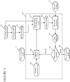
- FIG. 1 is a flowchart of a PS-RFWI process according to an embodiment.
- the PS-RFWI process has as inputs an initial S-velocity model 110, observed PS data 120, and a P-velocity model 130.
- the initial S-velocity model may be the result of one of the conventional methods mentioned in the background section or any other suitable approximation.
- Observed PS data has been separated from a seismic dataset acquired with multicomponent sensors as previously discussed.
- P-velocity model 130 may have been obtained, for example, by applying FWI to observed PP data separated from the same seismic dataset as observed PS data 120. However, P-velocity model 130 may also be the result of previously acquired seismic data or otherwise obtained.
- P-model velocity 130 is used to build a reflectivity model 134 by applying a true amplitude pre-stack depth migration (PSDM) method 132.
- PSDM true amplitude pre-stack depth migration
- Suitable methods of true amplitude PSDM include, for example, Kirchhoff true amplitude PSDM (described, e.g., by P. Whiting et al. in a 2001 article entitled, "Prestack Kirchhoff migration and amplitude accuracy," published as an Extended Abstract, ASEG 2001, Brisbane, pp. 1-4 ), one-way wave-equation true amplitude PSDM (described, e.g., by Y. Zhang et al.
- Rectangle 150 in Figure 1 emphasizes a portion of the PS-RFWI process that may be performed iteratively to minimize the difference between observed PS data 120 and synthetic data 160.
- Synthetic data 160 is generated at each iteration using Born modeling with reflectivity model, step 155, which receives as inputs: a current S-velocity model provided by PS-RFWI kernel 180, P-velocity model 130 and reflectivity model 134.
- the current S-velocity model is initial model 110 at the first iteration and an updated velocity model 185 at following iterations.
- the theoretical basis of Born modeling with reflectivity model is introduced below.
- Anisotropic wave propagation with acoustic approximation uses the wave equation.
- the subsurface of the Earth can be considered an anisotropic elastic media under the elastodynamic assumption (i.e., motion determined by linear elasticity).
- u i and f i are the i -th components of the particle displacement vector and the body force, respectively
- ⁇ is the density
- c ijkl is the ijkl -th component of the stiffness tensor, with indices i,j,k,l taking values between 1 and 3, and Einstein's summation convention over repeated indices being implied.
- step 165 data difference 170 between synthetic PS data 160 and observed PS data 120 is based on kinematic extraction 165.
- the theoretical basis of step 165 is detailed below.
- Synthetic PS data simulates incident P-wave converted into S-wave at an interface.
- U.S. Patent 10,310,123 which is incorporated herewith by reference, describes an FWI-based technique of updating a velocity model that splits the velocity model into a reference (also known as "background") model m 0 and a perturbation model ⁇ m .
- PS-RFWI uses a similar approach.
- Three model parameters describe the Born approximation of PS data: smooth background model of P- and S-wave velocity V p 0 , V s 0 , and a model perturbation ⁇ m .
- Equation (4) is not the exact formula for S-wave Born approximation. Therefore, the energy and scattering pattern of the secondary source differs from the true one. Thus, the forward modeled synthetic PS data does not have the same amplitudes as observed PS data. However, the demigration process based on equations (3)-(5) preserves the correct kinematic information of PS reflections.
- the PS-RFWI updates the S-velocity model using PS data by minimizing a cost function.
- Cost function J TT has good convexity to avoid the local minima during inversion, but its resolution and convergence rate is less than for the least-square cost function J LS .
- ⁇ d' (t + ⁇ ( ⁇ d , ⁇ d cal ( m 0 , ⁇ m ))) is an intermediate dataset generated by warping the synthetic data with a time shift ⁇ ⁇ ( ⁇ d, ⁇ d cal ( m 0 , ⁇ m )) between the synthetic and real data.
- the time shift ⁇ ⁇ ( ⁇ d, ⁇ d cal ( m 0 , ⁇ m )) can be determined, for example, using the dynamic warping method as described in the article entitled " Dynamic warping of seismic images" by D. Hale published in Geophysics, Vol. 78, no. 2, pp. S105-S115, 2013 (which is incorporated by reference), or a cross-correlation approach.
- the cost function J WD yields a better resolution and has a faster convergence rate than the cost function J TT without being affected by the amplitude mismatch.
- J can be any one of the cost functions in equations (6)-(9)
- the quantity ⁇ R represents the scattered adjoint wavefield and is obtained by demigration of the adjoint wavefield, R .
- the cross-correction between source side wavefield's derivative and receiver side wavefield is achieved by integration over time t up to the maximum record time tmax .
- each term of the gradient in equation (10) forms one side of the tomographic gradient (the so-called "rabbit ears" that are two branches in a graph representing the gradient in a vertical slice through the surveyed formation as in Figure 6D of U.S. Patent 10,310,123 ).
- PS-RFWI it is assumed that the P-wave processing has been completed, that is, V p 0 and PP reflectivity are accurate enough and fixed. This assumption means that only V s 0 is updated, and the first term of equation (10) is zero because P side wavefield of d cal is not related to V s 0 according to equation (3).
- Equation (11) means that only the S-side rabbit ear V s 0 (in a graph of gradient in a vertical slice through the surveyed underground formation mentioned above) is updated.
- the S-side rabbit ear represents the S-wave path where S-velocity changes affect the travel-time of S-wave. Therefore, it is important to single out the S-wave path for gradient calculation during the PS-RFWI.
- synthetic data 160 and observed data 120 kinematically matched at 165 yield data differences 170, that is, a cost function.
- a cost function As discussed above, an amplitude-discrepancy-mitigating (ADM) cost function that quantifies difference between the PS observed data and the PS synthetic data while alleviating an amplitude mismatch between the PS observed data and the PS synthetic data due to the use of the approximative acoustic equations is used. If, at 175, it is determined that cost function representing data residuals is a minimum according to a predetermined criterion (i.e., "TRUE" branch on 175), then the final S-velocity model 140 is output.
- a predetermined criterion i.e., "TRUE" branch on 175
- the predetermined criterion may be that the ADM cost function is less than a threshold or that its decrease from a previous iteration is less than a certain value.
- a predetermined number of iterations may be performed (i.e., the predetermined criterion is whether the current number of iterations equals the predetermined number of iterations).
- PS-RFWI kernel 180 If, however, at 175 it is determined that the ADM cost function can or should be further minimized, then PS-RFWI kernel 180 generates an updated S-velocity model 185 using the ADM cost function's derivative calculated according to formula (11) as further discussed below. The PS-RFWI kernel 180 then provides the updated S-velocity model 185 to step 155, where synthetic PS data 160 is regenerated for the next iteration.
- a short wavelength component of the velocity model or reflectivity is required to simulate the mode conversion at the sharp boundary (i.e., an interface where P-wave velocity changes suddenly and significantly) in the demigration process.
- the PP image i.e., P-velocity model
- the reflectivity may be based on either the PP image or the PS image.
- the PP image is preferred for obtaining reflectivity for the following reasons. First, PS data has quite limited illumination at shallow section because the S-wave velocity is slow (i.e., the PS image is inaccurate and has poor continuity in the shallow part, migration swings being concentrated around the receiver node), which makes the PS data demigration quite difficult.
- FIG. 1 illustrates an embodiment in which reflectivity is extracted from the PP image (i.e., P-velocity model) and remains the same at all the iterations.
- another embodiment may initially use the reflectivity is extracted from the PP image, but then at each iteration to extract reflectivity (to be used a next iteration) from an updated PS image.
- PS-RFWI Some embodiments of PS-RFWI are enhanced by using gradient interpolation as now explained.
- the S-wave is very slow near the water bottom. According to Snell's law, the S-wave's angle in these places is also very small, the S-wave propagating in the shallows close to the water bottom is nearly vertical. Therefore, the PS data provides very limited illumination in these regions, causing a poor horizontal resolution of S-wave model building.
- a gradient interpolation is performed to fill the gaps between the receiver nodes.
- the interpolation window length is determined by the receiver spacing and the model grid size used during the inversion.
- a sinc function-based interpolation may be used to spread the gradient into a smoothed version as illustrated in Figure 2(b) to mitigate this illumination problem.
- Figures 2(a) and 2(b) are vertical slices with depth on the vertical axis and a horizontal offset on the horizontal axis, the cost function's gradient being represented as nuances of gray.
- PS-RFWI may be achieved by using a preconditioner.
- a preconditioner may speed up convergence of the inversion.
- the precondition used in PP-RFWI links the gradient to the source illumination, making the pseudo Hessian to weight more on the deeper part during inversion as described in Gomes et. al.'s article entitled "Improving reflection FWI reflectivity using LSRTM in the curvelet domain” published in 2018 SEG International Exposition and 88th Annual Meeting, pp. 12481252 , which is incorporated herewith by reference.
- the gradient of RFWI requires a demigration process.
- the cross-correlation involves the adjoint wavefield R and the scattered wavefield ⁇ d cal .
- R decreases from the shallow to deep part
- ⁇ d cal increases from the shallow to deep part. Since the RFWI gradient is a combination of these two different diverging wavefields, the one-side illumination (source or receiver side) is not effective to increasing weigh for deeper layers of the S-wave velocity model. Therefore, different preconditioners are employed to amplify the deep part gradient.
- Preconditioners calculated with increasing values of n may be applied in different iterations, thereby simulating a layer-stripping strategy.
- Figures 3(a) and (b) illustrate gradient (represented as nuances of gray) calculations in vertical slices having 4,000 m depth and about 10,000 m horizontal range in the explored underground formation.
- Figures 4-7 are vertical slices of 5,000 m depth and about 20,000 m horizontal range.
- Figure 4 illustrates the P-wave velocity between 1,450 to 4,500 m/s illustrated as nuances of gray
- Figure 5 is the reflectivity (i.e., PP RTM image) corresponding to Figure 4.
- Figure 6 illustrates the S-wave velocity between 1,000 to 3,000 m/s illustrated also as nuances of gray (yet different nuances correspond here to different values than in Figure 4)
- Figure 7 is the reflectivity (i.e., PS RTM image) corresponding to Figure 6 .
- the PS-RFWI methods described in this section generate an S-wave velocity (Vs) model of an explored subsurface using PS data corresponding to the part of P-waves converted by reflection into S-waves.
- the anisotropic parameter of the S-wave ( ⁇ ') may also be updated during the same inversion.
- the P-wave velocity model and possible also the anisotropic parameter of the P-wave, ⁇ may be updated while keeping the S-wave part fixed.
- Equation (3)-(5) Using acoustic equations (equation (3)-(5)) for forward modeling of PS data preserves correct kinematic information although not correct amplitude compared to the real PS data.
- a cost function minimizing the travel-time difference ( ⁇ ) between the observed and modeled data may be used to mitigate the incorrect amplitude issue.
- this issue may be alleviated by minimizing waveform misfit between warped synthetic data and original synthetic PS data.
- the former mitigation strategy time lag minimization
- the very limited illumination of PS data in the shallow part is mitigated by gradient interpolation to fill the gaps between the receiver nodes, thereby avoiding the stripy gradient and/or poor horizontal resolution of S-wave model building.
- FIG 11 is a flowchart of a method 1100 for seismic exploration according to an embodiment.
- Method 1100 includes obtaining seismic data acquired using multicomponent sensors over a subsurface formation at 1110, and separating PS observed data from the seismic data at 1120.
- Multicomponent sensors enable detecting and separating both S-waves and P-waves after P-wave have been injected in the subsurface formation. Techniques of separating PS observed data from the seismic data have previously been discussed.
- Method 1100 then includes generating PS synthetic data using approximative acoustic equations in anisotropic media with a P-wave model, a current S-wave velocity model and a reflectivity model as inputs, at 1130 (as already disclosed) and updating the current S-wave velocity model using a full waveform inversion, FWI, to minimize an Amplitude-Discrepancy-Mitigating, ADM, cost function at 1140.
- the ADM cost function quantifies difference between the PS observed data and the PS synthetic data while alleviating an amplitude mismatch between the PS observed data and the PS synthetic data due to the use of the approximative acoustic equations.
- the ADM cost function is a sum of travel-time differences between the observed and the synthetic PS data (e.g., J TT in equation (8)). In another embodiment, the ADM cost function is a sum of differences between warped synthetic data and the synthetic data, the warped synthetic data being time shifted according to respective time shifts between the synthetic data and the observed data (e.g., J DW in equation (9)).
- Method 1100 further includes using the updated S-wave velocity model to assess presence of natural resources in the subsurface formation and/or to assist extraction of the natural resources from the subsurface formation at 1150.
- This step may include a comparison of a PP image-based reflectivity with a PS image-based reflectivity to identify fluid presence, and/or extracting information about areas under gas filled zones.
- steps 1130 and 1140 performed iteratively until a predetermined criterion related to ADM cost function's minimization is met.
- a predetermined criterion related to ADM cost function's minimization is met.
- an initial S-model being set as the current S-model at a first iteration and the updated S-wave velocity model being the current S-wave velocity model at a next iteration.
- the updating of the current S-wave velocity model may include calculating a cost function gradient with a gradient interpolation between receiver nodes.
- a preconditioner may be used when calculating the ADM cost function gradient.
- Observed PP data may also be separated from the seismic data and processed with RFWI or other methods to obtain the P-wave velocity model.
- the reflectivity model may be obtained by applying a true amplitude pre-stack depth migration method to the P-wave velocity model.
- One embodiment may further or additionally update an anisotropic parameter of S-wave, ⁇ ' using FWI.
- Another embodiment may update the P-wave velocity model while maintaining the current S-wave velocity model fixed.
- FIG. 12 shows a seismic data processing apparatus 1200 according to an embodiment.
- Apparatus 1200 is suitable for performing the above-described PS-RFWI seismic data processing.
- Server 1201 may include a central processor (CPU) 1202 and/or a graphic processor (GPU) coupled to a random-access memory (RAM) 1204 and to a read-only memory (ROM) 1206.
- ROM 1206 may also be other types of storage media to store programs, such as programmable ROM (PROM), erasable PROM (EPROM), etc.
- Processor 1202 may communicate with other internal and external components through input/output (I/O) circuitry 1208 and bussing 1210 to provide control signals and the like.
- I/O input/output
- Processor 1202 carries out a variety of functions as are known in the art, as dictated by software and/or firmware instructions.
- Server 1201 may also include one or more data storage devices, including hard drives 1212, CD-ROM drives 1214 and other hardware capable of reading and/or storing information, such as DVD, etc.
- software for carrying out the above-discussed steps may be stored and distributed on a CD-ROM or DVD 1216, a USB storage device 1218 or other form of media capable of portably storing information. These storage media may be inserted into, and read by, devices such as CD-ROM drive 1214, disk drive 1212, etc.
- Server 1201 may be coupled to a display 1220, which may be any type of known display or presentation screen, such as LCD, plasma display, cathode ray tube (CRT), etc.
- a user input interface 1222 is provided, including one or more user interface mechanisms such as a mouse, keyboard, microphone, touchpad, touch screen, voice-recognition system, etc.
- Server 1201 may be coupled to other devices, such as seismic sources, receivers, seismic data storage units, and may be part of a larger network configuration, such as in a global area network (GAN) like the internet 1228, which allows ultimate connection to various computing devices.
- GAN global area network
- RAM 1204 stores executable codes that, when executed, make processor 1202 perform the PS-RFWI methods according to various embodiments.
Landscapes
- Engineering & Computer Science (AREA)
- Remote Sensing (AREA)
- Physics & Mathematics (AREA)
- Life Sciences & Earth Sciences (AREA)
- Acoustics & Sound (AREA)
- Environmental & Geological Engineering (AREA)
- Geology (AREA)
- General Life Sciences & Earth Sciences (AREA)
- General Physics & Mathematics (AREA)
- Geophysics (AREA)
- Geophysics And Detection Of Objects (AREA)
Abstract
Description
- Embodiments of the subject matter disclosed herein generally relate to seismic exploration methods and devices using seismic data acquired with multicomponent sensors and due to P-waves injected in an explored underground formation; more specifically, to building an accurate S-wave velocity model of the explored underground formation from PS data extracted from seismic data.
- In recent years, multicomponent surveying has developed rapidly, especially with the quick deployment of ocean bottom seismic (OBS) acquisition. Data recorded by multicomponent sensors (e.g., including three orthogonal geophones or accelerometers) captures seismic wavefields emerging from the surveyed formations more completely than conventional sensors (e.g., single hydrophones, geophones or accelerometers). Note that sensors are sometimes called "receivers" or "detectors." These enhanced data acquisition abilities allow generating PS images resulting from downgoing P- (primary or compressional) waves being converted into upgoing S (secondary or shear) waves at their deepest point of penetration into the surveyed formation. That is, an incident P-wave at a solid-solid interface may generate a reflected P-wave, a transmitted P-wave, a reflected SV wave and a transmitted SV wave. Snell's Law governs the angular relationship between the rays of the resultant waves. SV waves are vertically polarized as opposed to SH waves, which are horizontally polarized. Since SH waves are not generated or detected when a P-wave source is used, the simpler term S-wave is sometimes used for SV waves resulting from converting the P-waves.
- S-waves are a useful tool for characterizing the elastic properties of a hydrocarbon reservoir for various reasons, such as, the comparison of P and S reflectivities enables better identification of fluid presence, and S-wave ray paths illuminate targets hidden beneath gas-filled zones. P- and S-waves provide complementary information that is helpful when inverting seismic data for determining elastic parameters of the explored formation's layers.
- Generating PS images is challenging because it requires consistent models for both P and S velocities since a P-wave is converted in a S-wave while traveling in the subsurface between the source and the sensor. FWI has proven to be a reliable tool for building accurate P-wave velocity (VP) models, but there is no conventional effective tool for building S-wave velocity (VS) models yet. PP and PS image registration or joint PP and PS tomography are conventionally used for converted S-wave velocity model updates. However, a conventionally obtained PS image is unreliable at shallow depths due to sparse acquisition of typical OBS surveys for PS registration, and tomography has limited resolution to deal with complex lateral velocity variations. VS model building for S-waves converted from incident P-waves has remained until now an unresolved challenge.
- The various embodiments described in this application provide an FWI-based approach to anisotropic VS velocity model building using acoustic equations for forward modeling (thereby, preserving kinematic information) and then a modified cost function mitigating the amplitude discrepancy between observed and simulated data.
- According to an embodiment, there is a method for seismic exploration that includes obtaining seismic data acquired using multicomponent sensors able to detect P-waves and S-waves emerging from a subsurface formation after P-waves have been injected therein. The method then includes separating PS observed data from the seismic data and generating PS synthetic data using approximative acoustic equations in anisotropic media with a P-wave model, a current S-wave velocity model and a reflectivity model as inputs. The method further includes updating the current S-wave velocity model using a full waveform inversion to minimize an amplitude-discrepancy-mitigating cost function quantifying difference between the PS observed data and the PS synthetic data while alleviating an amplitude mismatch between the PS observed data and the PS synthetic data due to the use of the approximative acoustic equations. The updated S-wave velocity model is then used to assess presence of natural resources in the subsurface formation and/or to assist extraction of the natural resources from the subsurface formation.
- According to another embodiment, there is a seismic data processing apparatus having an interface and a data processing unit connected to the interface. The interface is configured to obtain seismic data acquired using multicomponents sensors able to detect P-waves and S-waves emerging from a subsurface formation after P-waves have been injected therein. The data processing unit is configured to separate PS observed data from the seismic data, to generate PS synthetic data using approximative acoustic equations in anisotropic media with a P-wave model, a current S-wave velocity model and a reflectivity model as inputs, and to update the current S-wave velocity model using a full waveform inversion, FWI, to minimize an amplitude-discrepancy-mitigating, ADM, cost function quantifying difference between the PS observed data and the PS synthetic data while alleviating an amplitude mismatch between the PS observed data and the PS synthetic data due to the use of the approximative acoustic equations. The updated S-wave velocity model is usable to assess presence of natural resources in the subsurface formation and/or to assist extraction of the natural resources from the subsurface formation.
- According to yet another embodiment, there is a computer-readable recording medium non-transitorily storing executable codes that, when executed by a processor, make the processor perform a method for seismic exploration. The method includes obtaining seismic data acquired using multicomponent sensors able to detect P-waves and S-waves emerging from a subsurface formation after P-waves have been injected therein. The method then includes separating PS observed data from the seismic data and generating PS synthetic data using approximative acoustic equations in anisotropic media with a P-wave model, a current S-wave velocity model and a reflectivity model as inputs. The method further includes updating the current S-wave velocity model using a full waveform inversion to minimize an amplitude-discrepancy-mitigating cost function quantifying difference between the PS observed data and the PS synthetic data while alleviating an amplitude mismatch between the PS observed data and the PS synthetic data due to the use of the approximative acoustic equations. The updated S-wave velocity model is then used to assess presence of natural resources in the subsurface formation and/or to assist extraction of the natural resources from the subsurface formation.
- For a more complete understanding of the present inventive concept, reference is now made to the following descriptions taken in conjunction with the accompanying drawings, in which:
-
Figure 1 is a flowchart of a PS-RFWI process according to an embodiment; -
Figure 2(a) illustrates a gradient used to update the S-wave velocity model in a vertical slice before interpolation, andFigure 2(b) illustrates the gradient after interpolation; -
Figures 3(a) and 3(b) illustrate gradient calculations using different preconditioners; -
Figures 4-7 represent models and reflectivities characterizing synthetic OBS data used to test the PS-RFWI approach; -
Figure 8 illustrates the initial S-wave velocity model; -
Figure 9 represents the S-wave velocity model obtained using the PS-RFWI approach; -
Figure 10 represents reflectivity obtained using PS RTM based on the PS-RFWI results; and -
Figure 11 is flowchart of a method according to an embodiment; and -
Figure 12 is a schematic diagram of a seismic data processing apparatus according to an embodiment. - The following description of the exemplary embodiments refers to the accompanying drawings. The same reference numbers in different drawings identify the same or similar elements. The following detailed description does not limit the invention. Instead, the scope of the invention is defined by the appended claims. The following embodiments are discussed in the context of processing seismic data acquired with multicomponent sensors (enabling detection of both P-waves and S-waves) after P-waves are injected in an explored underground formation.
- Reference throughout the specification to "one embodiment" or "an embodiment" means that a particular feature, structure or characteristic described in connection with an embodiment is included in at least one embodiment of the subject matter disclosed. Thus, the phrases "in one embodiment" or "in an embodiment" in various places throughout the specification are not necessarily referring to the same embodiment. Further, the particular features, structures or characteristics may be combined in any suitable manner in one or more embodiments.
- The embodiments described in this section provide an FWI approach to generating an S-wave velocity model using PS seismic data. The multicomponent sensors record seismic data related to both P-waves and S-waves emerging from an explored underground formation in which P-waves have been injected (i.e., PP seismic data and PS seismic data). The incident P-waves are partially converted into S-waves at the deepest P-wave penetration reflection point. This approach is named PS-Reflection FWI (PS-RFWI) as it uses PS data (i.e., detected S-waves that have been generated from incident P-waves).
- Separating PS data and PP data (i.e., data corresponding to detected Sand P-waves from seismic data acquired with multicomponent sensors after P-waves have been injected into an explored subsurface formation) is a well-known technique. For example, in the article entitled "Separation of P- and S- Waves," by J.W.M. Dankbaar, published in Geophysical Prospecting 22, pp. 970-986, in 1985, Dankbaar sets forth a method using a separation filter with the coefficients determined from the near-surface PP and PS wave velocity and from the geometry of detecting geophone groups. Another article ("3D-PS Converted Waves - Solving 3D-imaging Challenges under Gas Clouds - Offshore Malaysia" by Akalin et al, published in 76th EAGE Conference & Exhibition, 2014) sets forth a practical flow for processing multicomponent sensor data acquired using ocean bottom sensors that use the fact that the S-waves often arrive at the surface nearly vertically, so that the near surface of the Earth acts as a natural P-wave versus S-wave separation filter. The PS data is then obtained from X and Y acceleration components subjected to tilt corrections, and then geometry rotations yielding radial and transverse motion components. The transverse component, which has very weak energy, is discarded and the radial component corresponding to detected S-waves is processed through noise attenuation, shear-wave statistics, demultiple, etc. The articles cited in this paragraph are incorporated by reference.
-
Figure 1 is a flowchart of a PS-RFWI process according to an embodiment. The PS-RFWI process has as inputs an initial S-velocity model 110, observedPS data 120, and a P-velocity model 130. The initial S-velocity model may be the result of one of the conventional methods mentioned in the background section or any other suitable approximation. Observed PS data has been separated from a seismic dataset acquired with multicomponent sensors as previously discussed. P-velocity model 130 may have been obtained, for example, by applying FWI to observed PP data separated from the same seismic dataset as observedPS data 120. However, P-velocity model 130 may also be the result of previously acquired seismic data or otherwise obtained. - P-
model velocity 130 is used to build areflectivity model 134 by applying a true amplitude pre-stack depth migration (PSDM)method 132. Suitable methods of true amplitude PSDM include, for example, Kirchhoff true amplitude PSDM (described, e.g., by P. Whiting et al. in a 2001 article entitled, "Prestack Kirchhoff migration and amplitude accuracy," published as an Extended Abstract, ASEG 2001, Brisbane, pp. 1-4), one-way wave-equation true amplitude PSDM (described, e.g., by Y. Zhang et al. in a 2007 article entitled, "True-amplitude, angle-domain, common-image gathers from one-way wave-equation migrations," published in Geophysics 72, No. 1, pp. S49-S58), controlled beam migration (CBM) true amplitude PSDM (described, e.g., by S. Gray et al. in a 2009 article entitled, "True-amplitude Gaussian-beam migration," published in Geophysics 74, No. 2, S11-S23), and reverse time migration, RTM, true amplitude PSDM (described, e.g., by Y. Zhang et al. in a 2013 article entitled, "Velocity and impedance inversion based true amplitude reverse time migration," published as an Extended Abstract in SEG 2013, pp. 949-953). All the papers mentioned in this paragraph are incorporated herewith by reference in their entirety. -
Rectangle 150 inFigure 1 emphasizes a portion of the PS-RFWI process that may be performed iteratively to minimize the difference betweenobserved PS data 120 andsynthetic data 160.Synthetic data 160 is generated at each iteration using Born modeling with reflectivity model,step 155, which receives as inputs: a current S-velocity model provided by PS-RFWI kernel 180, P-velocity model 130 andreflectivity model 134. The current S-velocity model isinitial model 110 at the first iteration and an updatedvelocity model 185 at following iterations. The theoretical basis of Born modeling with reflectivity model is introduced below. - Anisotropic wave propagation with acoustic approximation uses the wave equation. The subsurface of the Earth can be considered an anisotropic elastic media under the elastodynamic assumption (i.e., motion determined by linear elasticity). Seismic wave's propagation in such media is governed by the wave equation:

- Wave phenomena (such as transmission and reflection) in an anisotropic media are described by elastic wave equation (1) with P- and S-wave modes intrinsically coupled. However, since the P- and SV- waves are not generally polarized parallel and perpendicular to the wave vector, they are called quasi-P (qP) and quasi-S (qS) waves as discussed in the article entitled "Weak elastic anisotropy," by Thomsen, L. published in Geophysics, Vol. 51, pp. 1954-1966,1986, which is incorporated herewith by reference.
- The complex wave modes in the elastic wavefields, as well as the expensive computation cost, make it quite difficult to use the elastic wave equation (1). In order to save the computational cost, seismic data processing uses the acoustic approximation instead of equation (1). The article entitled "Simulating propagation of separated wave modes in general anisotropic media, Part I: qP-wave propagators," by J. Cheng et al., published in Geophysics 79, pp. C1-C18, 2014 (article which is incorporated herewith by reference), shows obtaining an acoustic wave equation in vertically transverse isotropic (VTI) media with shear wave velocity set to zero (see equation 23 therein):

P is the vector stress wavefield including horizontal and vertical components, ∂i (i=x,y,z) is spatial derivative along the i-th direction,F is the vector source term, ε and δ are the Thomsen parameters (introduced in the above-cited Thomsen article). This acoustic approximation can provide a kinematically correct anisotropic wavefield, which is accurate enough for most cases. For weak anisotropy cases, the q-SV wave also can be described by equation (2) with a set of equivalent Thomsen parameters:
- Returning now to
Figure 1 ,data difference 170 betweensynthetic PS data 160 and observedPS data 120 is based onkinematic extraction 165. The theoretical basis ofstep 165 is detailed below. - Synthetic PS data simulates incident P-wave converted into S-wave at an interface.
U.S. Patent 10,310,123 - Deriving PS data using equation (1) for a true amplitude Born modeling is too complicated for practical reasons. However, a good enough Born approximation of the amplitudes may be obtained using equation (2). The incident P-wave, P, propagates in the background model V p0 according to

- If this incident wavefield encounters a perturbation δ m, a secondary source


- Equation (4) is not the exact formula for S-wave Born approximation. Therefore, the energy and scattering pattern of the secondary source differs from the true one. Thus, the forward modeled synthetic PS data does not have the same amplitudes as observed PS data. However, the demigration process based on equations (3)-(5) preserves the correct kinematic information of PS reflections.
- The PS-RFWI updates the S-velocity model using PS data by minimizing a cost function. The generalized PS-RFWI cost function JREF (the Born approximation being used to generate the PS synthetic data) is:

- A particular form of JREF is the cost function used in the conventional least-squares FWI:

- As the amplitude is unreliably reproduced when the acoustic approximation is used, JLS may lead to severe errors during the inversion. Recently, other cost functions have been proposed. For example, a cost function JTT minimizes travel-time differences (Δτ) between observed and synthetic PS data:

- Cost function JTT has good convexity to avoid the local minima during inversion, but its resolution and convergence rate is less than for the least-square cost function JLS.
- Another cost function JWD that aims to mitigate amplitude mismatch is using warped data:

- Since RFWI aims to update the reference/background models (e.g., V s0 , V p0 , δ'), the gradient may be calculated by simply taking the derivative of the cost function with respect to a respective background/reference model m0 :

- In the PP-RFWI, each term of the gradient in equation (10) forms one side of the tomographic gradient (the so-called "rabbit ears" that are two branches in a graph representing the gradient in a vertical slice through the surveyed formation as in
Figure 6D ofU.S. Patent 10,310,123 
- Equation (11) means that only the S-side rabbit ear V s0 (in a graph of gradient in a vertical slice through the surveyed underground formation mentioned above) is updated. In fact, the S-side rabbit ear represents the S-wave path where S-velocity changes affect the travel-time of S-wave. Therefore, it is important to single out the S-wave path for gradient calculation during the PS-RFWI. The anisotropic parameter of S-wave, δ', can be similarly updated using the following gradient:

- Similarly, if S-wave velocity may be considered fixed and one focuses on the P-side wave path, the P-wave velocity model may be updated using:

- Returning again to
Figure 1 ,synthetic data 160 and observeddata 120 kinematically matched at 165yield data differences 170, that is, a cost function. As discussed above, an amplitude-discrepancy-mitigating (ADM) cost function that quantifies difference between the PS observed data and the PS synthetic data while alleviating an amplitude mismatch between the PS observed data and the PS synthetic data due to the use of the approximative acoustic equations is used. If, at 175, it is determined that cost function representing data residuals is a minimum according to a predetermined criterion (i.e., "TRUE" branch on 175), then the final S-velocity model 140 is output. The predetermined criterion may be that the ADM cost function is less than a threshold or that its decrease from a previous iteration is less than a certain value. Alternatively, a predetermined number of iterations may be performed (i.e., the predetermined criterion is whether the current number of iterations equals the predetermined number of iterations). - If, however, at 175 it is determined that the ADM cost function can or should be further minimized, then PS-
RFWI kernel 180 generates an updated S-velocity model 185 using the ADM cost function's derivative calculated according to formula (11) as further discussed below. The PS-RFWI kernel 180 then provides the updated S-velocity model 185 to step 155, wheresynthetic PS data 160 is regenerated for the next iteration. - A short wavelength component of the velocity model or reflectivity is required to simulate the mode conversion at the sharp boundary (i.e., an interface where P-wave velocity changes suddenly and significantly) in the demigration process. In conventional PP-RFWI, the PP image (i.e., P-velocity model) generated by, for example, reverse time migration is used for reflectivity. In PS-RFWI, the reflectivity may be based on either the PP image or the PS image. The PP image is preferred for obtaining reflectivity for the following reasons. First, PS data has quite limited illumination at shallow section because the S-wave velocity is slow (i.e., the PS image is inaccurate and has poor continuity in the shallow part, migration swings being concentrated around the receiver node), which makes the PS data demigration quite difficult. Second, P-wave processing can provide a good Vp model and well-located PP image, making it possible to mitigate the ambiguity of depth and velocity in the PS reflection data inversion (unlike in the PP-RFWI where the ambiguity of the depth and velocity are quite hard to resolve).
Figure 1 illustrates an embodiment in which reflectivity is extracted from the PP image (i.e., P-velocity model) and remains the same at all the iterations. However, another embodiment may initially use the reflectivity is extracted from the PP image, but then at each iteration to extract reflectivity (to be used a next iteration) from an updated PS image. - Some embodiments of PS-RFWI are enhanced by using gradient interpolation as now explained. The S-wave is very slow near the water bottom. According to Snell's law, the S-wave's angle in these places is also very small, the S-wave propagating in the shallows close to the water bottom is nearly vertical. Therefore, the PS data provides very limited illumination in these regions, causing a poor horizontal resolution of S-wave model building. To avoid the stripy gradient as in
Figure 2(a) , a gradient interpolation is performed to fill the gaps between the receiver nodes. The interpolation window length is determined by the receiver spacing and the model grid size used during the inversion. A sinc function-based interpolation may be used to spread the gradient into a smoothed version as illustrated inFigure 2(b) to mitigate this illumination problem.Figures 2(a) and 2(b) are vertical slices with depth on the vertical axis and a horizontal offset on the horizontal axis, the cost function's gradient being represented as nuances of gray. - Another improvement of PS-RFWI may be achieved by using a preconditioner. As known from PP-RFWI, a preconditioner may speed up convergence of the inversion. The precondition used in PP-RFWI links the gradient to the source illumination, making the pseudo Hessian to weight more on the deeper part during inversion as described in Gomes et. al.'s article entitled "Improving reflection FWI reflectivity using LSRTM in the curvelet domain" published in 2018 SEG International Exposition and 88th Annual Meeting, pp. 12481252, which is incorporated herewith by reference. However, the gradient of RFWI requires a demigration process. In equation (11), the cross-correlation involves the adjoint wavefield R and the scattered wavefield δdcal . Here, R decreases from the shallow to deep part, while δdcal increases from the shallow to deep part. Since the RFWI gradient is a combination of these two different diverging wavefields, the one-side illumination (source or receiver side) is not effective to increasing weigh for deeper layers of the S-wave velocity model. Therefore, different preconditioners are employed to amplify the deep part gradient. For example, a preconditioner H may be used to amplify the deep part of the gradient, resulting in a preconditioned gradient g according to the following formulas:


Figures 3(a) and (b) illustrate gradient (represented as nuances of gray) calculations in vertical slices having 4,000 m depth and about 10,000 m horizontal range in the explored underground formation. A preconditioner corresponding to n=1 was used for the gradient calculation illustrated inFigure 3(a) , and a preconditioner corresponding to n=2 was used for the gradient calculation illustrated inFigure 3(b) . - The above-described approach was tested on synthetic OBS data. The synthetic test data is characterized by
Figures 4-7 , which are vertical slices of 5,000 m depth and about 20,000 m horizontal range.Figure 4 illustrates the P-wave velocity between 1,450 to 4,500 m/s illustrated as nuances of gray, andFigure 5 is the reflectivity (i.e., PP RTM image) corresponding toFigure 4. Figure 6 illustrates the S-wave velocity between 1,000 to 3,000 m/s illustrated also as nuances of gray (yet different nuances correspond here to different values than inFigure 4), and Figure 7 is the reflectivity (i.e., PS RTM image) corresponding toFigure 6 . - Then starting from an initial S-wave velocity model as illustrated in
Figure 8 , the S-wave velocity model inFigure 9 with a reflectivity (PS RTM image) as illustrated inFigure 10 is obtained using the above-described PS-RFWI. - Thus, the PS-RFWI methods described in this section generate an S-wave velocity (Vs) model of an explored subsurface using PS data corresponding to the part of P-waves converted by reflection into S-waves. The anisotropic parameter of the S-wave (δ') may also be updated during the same inversion. Conversely, once the S-wave velocity model and a corresponding reflectivity image are available, the P-wave velocity model (and possible also the anisotropic parameter of the P-wave, δ) may be updated while keeping the S-wave part fixed.
- Using acoustic equations (equation (3)-(5)) for forward modeling of PS data preserves correct kinematic information although not correct amplitude compared to the real PS data. A cost function minimizing the travel-time difference (Δτ) between the observed and modeled data may be used to mitigate the incorrect amplitude issue. Alternatively, this issue may be alleviated by minimizing waveform misfit between warped synthetic data and original synthetic PS data. The former mitigation strategy (time lag minimization) has good convexity to avoid local minima during inversion but less resolution and a slower convergence rate than the latter strategy using a waveform-based cost function.
- The very limited illumination of PS data in the shallow part is mitigated by gradient interpolation to fill the gaps between the receiver nodes, thereby avoiding the stripy gradient and/or poor horizontal resolution of S-wave model building.
-
Figure 11 is a flowchart of amethod 1100 for seismic exploration according to an embodiment.Method 1100 includes obtaining seismic data acquired using multicomponent sensors over a subsurface formation at 1110, and separating PS observed data from the seismic data at 1120. Multicomponent sensors enable detecting and separating both S-waves and P-waves after P-wave have been injected in the subsurface formation. Techniques of separating PS observed data from the seismic data have previously been discussed. -
Method 1100 then includes generating PS synthetic data using approximative acoustic equations in anisotropic media with a P-wave model, a current S-wave velocity model and a reflectivity model as inputs, at 1130 (as already disclosed) and updating the current S-wave velocity model using a full waveform inversion, FWI, to minimize an Amplitude-Discrepancy-Mitigating, ADM, cost function at 1140. The ADM cost function quantifies difference between the PS observed data and the PS synthetic data while alleviating an amplitude mismatch between the PS observed data and the PS synthetic data due to the use of the approximative acoustic equations. - In one embodiment, the ADM cost function is a sum of travel-time differences between the observed and the synthetic PS data (e.g., JTT in equation (8)). In another embodiment, the ADM cost function is a sum of differences between warped synthetic data and the synthetic data, the warped synthetic data being time shifted according to respective time shifts between the synthetic data and the observed data (e.g., JDW in equation (9)).
-
Method 1100 further includes using the updated S-wave velocity model to assess presence of natural resources in the subsurface formation and/or to assist extraction of the natural resources from the subsurface formation at 1150. This step may include a comparison of a PP image-based reflectivity with a PS image-based reflectivity to identify fluid presence, and/or extracting information about areas under gas filled zones. - As suggested by the dashed arrow,
steps - As already discussed, the updating of the current S-wave velocity model may include calculating a cost function gradient with a gradient interpolation between receiver nodes. A preconditioner may be used when calculating the ADM cost function gradient.
- Observed PP data may also be separated from the seismic data and processed with RFWI or other methods to obtain the P-wave velocity model. The reflectivity model may be obtained by applying a true amplitude pre-stack depth migration method to the P-wave velocity model.
- One embodiment may further or additionally update an anisotropic parameter of S-wave, δ' using FWI. Another embodiment may update the P-wave velocity model while maintaining the current S-wave velocity model fixed.
-
Figure 12 shows a seismicdata processing apparatus 1200 according to an embodiment.Apparatus 1200 is suitable for performing the above-described PS-RFWI seismic data processing.Server 1201 may include a central processor (CPU) 1202 and/or a graphic processor (GPU) coupled to a random-access memory (RAM) 1204 and to a read-only memory (ROM) 1206.ROM 1206 may also be other types of storage media to store programs, such as programmable ROM (PROM), erasable PROM (EPROM), etc.Processor 1202 may communicate with other internal and external components through input/output (I/O)circuitry 1208 and bussing 1210 to provide control signals and the like.Processor 1202 carries out a variety of functions as are known in the art, as dictated by software and/or firmware instructions. -
Server 1201 may also include one or more data storage devices, includinghard drives 1212, CD-ROM drives 1214 and other hardware capable of reading and/or storing information, such as DVD, etc. In one embodiment, software for carrying out the above-discussed steps may be stored and distributed on a CD-ROM orDVD 1216, aUSB storage device 1218 or other form of media capable of portably storing information. These storage media may be inserted into, and read by, devices such as CD-ROM drive 1214,disk drive 1212, etc.Server 1201 may be coupled to a display 1220, which may be any type of known display or presentation screen, such as LCD, plasma display, cathode ray tube (CRT), etc. Auser input interface 1222 is provided, including one or more user interface mechanisms such as a mouse, keyboard, microphone, touchpad, touch screen, voice-recognition system, etc. -
Server 1201 may be coupled to other devices, such as seismic sources, receivers, seismic data storage units, and may be part of a larger network configuration, such as in a global area network (GAN) like theinternet 1228, which allows ultimate connection to various computing devices. - In yet another embodiment,
RAM 1204 stores executable codes that, when executed, makeprocessor 1202 perform the PS-RFWI methods according to various embodiments. - The disclosed embodiments provide PS-RFWI methods and apparatuses for processing seismic data acquired using multicomponent sensors. It should be understood that this description is not intended to limit the invention. On the contrary, the embodiments are intended to cover alternatives, modifications and equivalents, which are included in the spirit and scope of the invention as defined by the appended claims. Further, in the detailed description of the embodiments, numerous specific details are set forth in order to provide a comprehensive understanding of the claimed invention. However, one skilled in the art would understand that various embodiments may be practiced without such specific details.
- Although the features and elements of the present embodiments are described in the embodiments in particular combinations, each feature or element can be used alone without the other features and elements of the embodiments or in various combinations with or without other features and elements disclosed herein.
- This written description uses examples of the subject matter disclosed to enable any person skilled in the art to practice the same, including making and using any devices or systems and performing any incorporated methods. The patentable scope of the subject matter is defined by the claims, and may include other examples that occur to those skilled in the art. Such other examples are intended to be within the scope of the claims.
Claims (15)
- A method (1100) for seismic exploration, the method comprising:obtaining (1110) seismic data acquired using multicomponent sensors able to detect P-waves and S-waves emerging from a subsurface formation after P-waves have been injected therein;separating (1120) PS observed data from the seismic data;generating (1130) PS synthetic data using approximative acoustic equations in anisotropic media with a P-wave model, a current S-wave velocity model and a reflectivity model as inputs;updating (1140) the current S-wave velocity model using a full waveform inversion, FWI, to minimize an amplitude-discrepancy-mitigating, ADM, cost function quantifying difference between the PS observed data and the PS synthetic data while alleviating an amplitude mismatch between the PS observed data and the PS synthetic data due to the use of the approximative acoustic equations; andusing (1150) the updated S-wave velocity model to assess presence of natural resources in the subsurface formation and/or to assist extraction of the natural resources from the subsurface formation.
- The method of claim 1, wherein the generating of the PS synthetic data and the updating of the current S-wave velocity model are performed iteratively until a predetermined criterion related to ADM cost function's minimization is met, an initial S-model being set as the current S-model at a first iteration and the updated S-wave velocity model being the current S-wave velocity model at a next iteration.
- The method of claim 1, wherein the ADM cost function is a sum of travel-time differences between the observed and the synthetic PS data.
- The method of claim 1, wherein the ADM cost function is a sum of differences between warped synthetic data and the synthetic data, the warped synthetic data being time shifted according to respective time shifts between the synthetic data and the observed data.
- The method of claim 1, wherein the updating of the current S-wave velocity model includes calculating a cost function gradient with a gradient interpolation between receiver nodes.
- The method of claim 5, wherein an interpolation window length is determined according to receiver spacing and size of model grid used by the FWI.
- The method of claim 5, wherein the gradient interpolation uses a sinc function.
- The method of claim 1, wherein the updating of the current S-wave velocity model includes calculating a cost function gradient that uses a preconditioner.
- The method of claim 1, wherein observed PP data are also separated from the seismic data, the method further comprising generating the P-wave velocity model based on the observed PP data.
- The method of claim 1, further comprising:
obtaining the reflectivity model by applying a true amplitude pre-stack depth migration method to the P-wave velocity model. - The method of claim 1, wherein the using of the updated S-wave velocity model includes a comparison of a PP image-based reflectivity with a PS image-based reflectivity to identify fluid presence, and/or extracting information about areas under gas filled zones.
- The method of claim 1, further comprising:
updating an anisotropic parameter of S-wave, δ' using FWI. - The method of claim 1, further comprising:
updating the P-wave velocity model while maintaining the current S-wave velocity model fixed. - A seismic data processing apparatus (1200), comprising:an interface (1208) configured to obtain seismic data acquired using multicomponents sensors able to detect P-waves and S-waves emerging from a subsurface formation after P-waves have been injected therein; anda data processing unit (1202) connected to the interface and configuredto separate PS observed data from the seismic data;to generate PS synthetic data using approximative acoustic equations in anisotropic media with a P-wave model, a current S-wave velocity model and a reflectivity model as inputs; andto update the current S-wave velocity model using a full waveform inversion, FWI, to minimize an amplitude-discrepancy-mitigating, ADM, cost function quantifying difference between the PS observed data and the PS synthetic data while alleviating an amplitude mismatch between the PS observed data and the PS synthetic data due to the use of the approximative acoustic equations,wherein the updated S-wave velocity model is usable to assess presence of natural resources in the subsurface formation and/or to assist extraction of the natural resources from the subsurface formation.
- A non-transitory computer readable medium (1204) storing executable codes which, when executed on a computer (1201) make the computer perform a method (1100) for seismic exploration comprising:obtaining (1110) seismic data acquired using multicomponent sensors able to detect P-waves and S-waves emerging from a subsurface formation after P-waves have been injected therein;separating (1120) PS observed data from the seismic data;generating (1130) PS synthetic data using approximative acoustic equations in anisotropic media with a P-wave model, a current S-wave velocity model and a reflectivity model as inputs;updating (1140) the current S-wave velocity model using a full waveform inversion, FWI, to minimize an amplitude-discrepancy-mitigating, ADM, cost function quantifying difference between the PS observed data and the PS synthetic data while alleviating an amplitude mismatch between the PS observed data and the PS synthetic data due to the use of the approximative acoustic equations; andusing (1150) the updated S-wave velocity model to assess presence of natural resources in the subsurface formation and/or to assist extraction of the natural resources from the subsurface formation.
Applications Claiming Priority (1)
| Application Number | Priority Date | Filing Date | Title |
|---|---|---|---|
| US201962869101P | 2019-07-01 | 2019-07-01 |
Publications (2)
| Publication Number | Publication Date |
|---|---|
| EP3761067A1 true EP3761067A1 (en) | 2021-01-06 |
| EP3761067B1 EP3761067B1 (en) | 2024-04-17 |
Family
ID=71266532
Family Applications (1)
| Application Number | Title | Priority Date | Filing Date |
|---|---|---|---|
| EP20305552.0A Active EP3761067B1 (en) | 2019-07-01 | 2020-05-27 | Full waveform inversion approach to building an s-wave velocity model using ps data |
Country Status (3)
| Country | Link |
|---|---|
| US (1) | US11215720B2 (en) |
| EP (1) | EP3761067B1 (en) |
| MX (1) | MX2020005379A (en) |
Cited By (1)
| Publication number | Priority date | Publication date | Assignee | Title |
|---|---|---|---|---|
| EP4165444A4 (en) * | 2020-06-11 | 2024-06-05 | Dug Technology (Australia) Pty Ltd | Seismic wavefield modeling honoring avo/ava with applications to full waveform inversion and least-squares imaging |
Families Citing this family (8)
| Publication number | Priority date | Publication date | Assignee | Title |
|---|---|---|---|---|
| US11747499B2 (en) * | 2021-01-14 | 2023-09-05 | Cgg Services Sas | Full-waveform inversion using partial time shifts and enhanced kinematic transforms |
| US11867856B2 (en) | 2021-06-03 | 2024-01-09 | Saudi Arabian Oil Company | Method and system for reflection-based travel time inversion using segment dynamic image warping |
| US11668848B2 (en) * | 2021-06-24 | 2023-06-06 | Saudi Arabian Oil Company | Method and system for seismic imaging using S-wave velocity models and machine learning |
| US12352915B2 (en) | 2022-10-28 | 2025-07-08 | Saudi Arabian Oil Company | Method and system for estimating converted-wave statics |
| US20240310544A1 (en) * | 2023-03-15 | 2024-09-19 | Cgg Services Sas | Domain decomposition for high-frequency elastic full waveform inversion method and system |
| US20240319394A1 (en) * | 2023-03-24 | 2024-09-26 | Cgg Services Sas | Complex wavelet based full waveform inversion method and system for processing seismic data |
| CN120214895B (en) * | 2025-05-07 | 2026-04-17 | 成都理工大学 | Ground stress azimuth earthquake prediction method based on transverse wave velocity change rate |
| CN121008320B (en) * | 2025-08-19 | 2026-04-17 | 成都深地科技有限公司 | Small geologic body fine imaging method based on FWI technology |
Citations (3)
| Publication number | Priority date | Publication date | Assignee | Title |
|---|---|---|---|---|
| US20170168177A1 (en) * | 2015-12-11 | 2017-06-15 | Ion Geophysical Corporation | System and method for reconstructed wavefield inversion |
| CN108845351A (en) * | 2018-06-26 | 2018-11-20 | 中国石油大学(华东) | A kind of VSP seismic data converted wave full waveform inversion method |
| US10310123B2 (en) | 2012-03-09 | 2019-06-04 | Cgg Services Sas | Seismic reflection full waveform inversion for reflected seismic data |
Family Cites Families (3)
| Publication number | Priority date | Publication date | Assignee | Title |
|---|---|---|---|---|
| WO2010085493A1 (en) * | 2009-01-20 | 2010-07-29 | Spectraseis Ag | Time reverse imaging operators for source location |
| GB2554865B (en) * | 2016-10-04 | 2021-10-20 | Equinor Energy As | Seismic modeling |
| US11353613B2 (en) | 2017-11-17 | 2022-06-07 | Cgg Services Sas | Seismic exploration using image-based reflection full waveform inversion to update low wavenumber velocity model |
-
2020
- 2020-05-08 US US16/870,274 patent/US11215720B2/en active Active
- 2020-05-27 EP EP20305552.0A patent/EP3761067B1/en active Active
- 2020-07-13 MX MX2020005379A patent/MX2020005379A/en unknown
Patent Citations (3)
| Publication number | Priority date | Publication date | Assignee | Title |
|---|---|---|---|---|
| US10310123B2 (en) | 2012-03-09 | 2019-06-04 | Cgg Services Sas | Seismic reflection full waveform inversion for reflected seismic data |
| US20170168177A1 (en) * | 2015-12-11 | 2017-06-15 | Ion Geophysical Corporation | System and method for reconstructed wavefield inversion |
| CN108845351A (en) * | 2018-06-26 | 2018-11-20 | 中国石油大学(华东) | A kind of VSP seismic data converted wave full waveform inversion method |
Non-Patent Citations (12)
| Title |
|---|
| AKALIN ET AL.: "3D-PS Converted Waves - Solving 3D-imaging Challenges under Gas Clouds - Offshore Malaysia", 76TH EAGE CONFERENCE & EXHIBITION, 2014 |
| D. HALE: "Dynamic warping of seismic images", GEOPHYSICS, vol. 78, no. 2, 2013, pages S105 - S115, XP001580878, DOI: 10.1190/geo2012-0327.1 |
| GOMES: "Improving reflection FWI reflectivity using LSRTM in the curvelet domain", SEG INTERNATIONAL EXPOSITION AND 88TH ANNUAL MEETING, 2018, pages 12481252 |
| J. CHENG ET AL.: "Simulating propagation of separated wave modes in general anisotropic media, Part I: qP-wave propagators", GEOPHYSICS, vol. 79, 2014, pages C1 - C18, XP001587321, DOI: 10.1190/geo2012-0504.1 |
| J.W.M. DANKBAAR: "Separation of P- and S- Waves", GEOPHYSICAL PROSPECTING, vol. 22, 1985, pages 970 - 986 |
| P. WHITING ET AL.: "Prestack Kirchhoff migration and amplitude accuracy", EXTENDED ABSTRACT, ASEG 2001, 2001, pages 1 - 4 |
| S. GRAY ET AL.: "True-amplitude Gaussian-beam migration", GEOPHYSICS, vol. 74, no. 2, 2009, pages S11 - S23, XP001520862, DOI: 10.1190/1.3052116 |
| TARIQ ALKHALIFAH: "An acoustic wave equation for anisotropic media", GEOPHYSICS, 1 January 2000 (2000-01-01), pages 1239 - 1250, XP055308539, Retrieved from the Internet <URL:http://library.seg.org/doi/pdf/10.1190/1.1444815> DOI: 10.1190/1.1444815 * |
| THOMSEN, L.: "Weak elastic anisotropy", GEOPHYSICS, vol. 51, 1986, pages 1954 - 1966, XP002703266, DOI: 10.1190/1.1442051 |
| VIRIEUX J ET AL: "An overview of full-waveform inversion in exploration geophysics", GEOPHYSICS, SOCIETY OF EXPLORATION GEOPHYSICISTS, US, vol. 74, no. Suppl. of 6, 1 November 2009 (2009-11-01), pages WCC1 - WCC26, XP001550475, ISSN: 0016-8033, DOI: 10.1190/1.3238367 * |
| Y. ZHANG ET AL.: "True-amplitude, angle-domain, common-image gathers from one-way wave-equation migrations", GEOPHYSICS, vol. 72, no. 1, 2007, pages S49 - S58, XP001503465, DOI: 10.1190/1.2399371 |
| Y. ZHANG ET AL.: "Velocity and impedance inversion based true amplitude reverse time migration", EXTENDED ABSTRACT IN SEG 2013, 2013, pages 949 - 953 |
Cited By (1)
| Publication number | Priority date | Publication date | Assignee | Title |
|---|---|---|---|---|
| EP4165444A4 (en) * | 2020-06-11 | 2024-06-05 | Dug Technology (Australia) Pty Ltd | Seismic wavefield modeling honoring avo/ava with applications to full waveform inversion and least-squares imaging |
Also Published As
| Publication number | Publication date |
|---|---|
| MX2020005379A (en) | 2021-01-04 |
| US20210003728A1 (en) | 2021-01-07 |
| EP3761067B1 (en) | 2024-04-17 |
| BR102020012059A2 (en) | 2021-09-08 |
| US11215720B2 (en) | 2022-01-04 |
Similar Documents
| Publication | Publication Date | Title |
|---|---|---|
| EP3761067B1 (en) | Full waveform inversion approach to building an s-wave velocity model using ps data | |
| US11048001B2 (en) | Methods using travel-time full waveform inversion for imaging subsurface formations with salt bodies | |
| US11353613B2 (en) | Seismic exploration using image-based reflection full waveform inversion to update low wavenumber velocity model | |
| US11487036B2 (en) | Reflection full waveform inversion methods with density and velocity models updated separately | |
| Guasch et al. | Adaptive waveform inversion: Practice | |
| Vigh et al. | 3D prestack plane-wave, full-waveform inversion | |
| EP4042210B1 (en) | Determining properties of a subterranean formation using an acoustic wave equation with a reflectivity parameterization | |
| Ravasi et al. | Elastic imaging with exact wavefield extrapolation for application to ocean-bottom 4C seismic data | |
| US7508736B2 (en) | Vector migration of 1st order free-surface related downgoing multiples from VSP data | |
| US20130311151A1 (en) | Earth model estimation through an acoustic full waveform inversion of seismic data | |
| US20130289879A1 (en) | Process for characterising the evolution of a reservoir | |
| Wang et al. | Inversion of seismic refraction and reflection data for building long-wavelength velocity models | |
| Witten et al. | Extended wave-equation imaging conditions for passive seismic data | |
| US20130176823A1 (en) | Simultaneous joint estimation of the p-p and p-s residual statics | |
| US12320937B2 (en) | Full-waveform inversion with elastic mitigation using acoustic anisotropy | |
| US11635540B2 (en) | Methods and devices performing adaptive quadratic Wasserstein full-waveform inversion | |
| Warner et al. | Automated salt model building: From compaction trend to final velocity model using waveform inversion | |
| Wang et al. | Converted-wave reflection traveltime inversion with free-surface multiples for ocean-bottom-node data | |
| Cho et al. | Laplace–Fourier-domain full waveform inversion of deep-sea seismic data acquired with limited offsets | |
| US20240069233A1 (en) | Seismic data processing using a down-going annihilation operator | |
| US12560732B2 (en) | Dynamic resolution full-waveform inversion method and system | |
| Cocher | Iterative migration velocity analysis: Extension to surface-related multiple reflections | |
| Zuniga | Nonhyperbolic multiparametric travel-time approximation for converted-wave and OBN data | |
| US11940579B2 (en) | Method and system using wave-equation for obtaining traveltime and amplitude used in Kirchhoff migration | |
| He et al. | Joint PP/PS tomography with dynamic warping |
Legal Events
| Date | Code | Title | Description |
|---|---|---|---|
| PUAI | Public reference made under article 153(3) epc to a published international application that has entered the european phase |
Free format text: ORIGINAL CODE: 0009012 |
|
| STAA | Information on the status of an ep patent application or granted ep patent |
Free format text: STATUS: THE APPLICATION HAS BEEN PUBLISHED |
|
| AK | Designated contracting states |
Kind code of ref document: A1 Designated state(s): AL AT BE BG CH CY CZ DE DK EE ES FI FR GB GR HR HU IE IS IT LI LT LU LV MC MK MT NL NO PL PT RO RS SE SI SK SM TR |
|
| AX | Request for extension of the european patent |
Extension state: BA ME |
|
| STAA | Information on the status of an ep patent application or granted ep patent |
Free format text: STATUS: REQUEST FOR EXAMINATION WAS MADE |
|
| 17P | Request for examination filed |
Effective date: 20210512 |
|
| RBV | Designated contracting states (corrected) |
Designated state(s): AL AT BE BG CH CY CZ DE DK EE ES FI FR GB GR HR HU IE IS IT LI LT LU LV MC MK MT NL NO PL PT RO RS SE SI SK SM TR |
|
| STAA | Information on the status of an ep patent application or granted ep patent |
Free format text: STATUS: EXAMINATION IS IN PROGRESS |
|
| 17Q | First examination report despatched |
Effective date: 20220824 |
|
| P01 | Opt-out of the competence of the unified patent court (upc) registered |
Effective date: 20230530 |
|
| GRAP | Despatch of communication of intention to grant a patent |
Free format text: ORIGINAL CODE: EPIDOSNIGR1 |
|
| STAA | Information on the status of an ep patent application or granted ep patent |
Free format text: STATUS: GRANT OF PATENT IS INTENDED |
|
| INTG | Intention to grant announced |
Effective date: 20231128 |
|
| GRAS | Grant fee paid |
Free format text: ORIGINAL CODE: EPIDOSNIGR3 |
|
| GRAA | (expected) grant |
Free format text: ORIGINAL CODE: 0009210 |
|
| STAA | Information on the status of an ep patent application or granted ep patent |
Free format text: STATUS: THE PATENT HAS BEEN GRANTED |
|
| AK | Designated contracting states |
Kind code of ref document: B1 Designated state(s): AL AT BE BG CH CY CZ DE DK EE ES FI FR GB GR HR HU IE IS IT LI LT LU LV MC MK MT NL NO PL PT RO RS SE SI SK SM TR |
|
| REG | Reference to a national code |
Ref country code: GB Ref legal event code: FG4D |
|
| REG | Reference to a national code |
Ref country code: CH Ref legal event code: EP |
|
| REG | Reference to a national code |
Ref country code: DE Ref legal event code: R096 Ref document number: 602020029108 Country of ref document: DE |
|
| REG | Reference to a national code |
Ref country code: IE Ref legal event code: FG4D |
|
| REG | Reference to a national code |
Ref country code: LT Ref legal event code: MG9D |
|
| REG | Reference to a national code |
Ref country code: NL Ref legal event code: MP Effective date: 20240417 |
|
| REG | Reference to a national code |
Ref country code: AT Ref legal event code: MK05 Ref document number: 1677765 Country of ref document: AT Kind code of ref document: T Effective date: 20240417 |
|
| PG25 | Lapsed in a contracting state [announced via postgrant information from national office to epo] |
Ref country code: NL Free format text: LAPSE BECAUSE OF FAILURE TO SUBMIT A TRANSLATION OF THE DESCRIPTION OR TO PAY THE FEE WITHIN THE PRESCRIBED TIME-LIMIT Effective date: 20240417 |
|
| PG25 | Lapsed in a contracting state [announced via postgrant information from national office to epo] |
Ref country code: NL Free format text: LAPSE BECAUSE OF FAILURE TO SUBMIT A TRANSLATION OF THE DESCRIPTION OR TO PAY THE FEE WITHIN THE PRESCRIBED TIME-LIMIT Effective date: 20240417 |
|
| PG25 | Lapsed in a contracting state [announced via postgrant information from national office to epo] |
Ref country code: IS Free format text: LAPSE BECAUSE OF FAILURE TO SUBMIT A TRANSLATION OF THE DESCRIPTION OR TO PAY THE FEE WITHIN THE PRESCRIBED TIME-LIMIT Effective date: 20240817 |
|
| PG25 | Lapsed in a contracting state [announced via postgrant information from national office to epo] |
Ref country code: BG Free format text: LAPSE BECAUSE OF FAILURE TO SUBMIT A TRANSLATION OF THE DESCRIPTION OR TO PAY THE FEE WITHIN THE PRESCRIBED TIME-LIMIT Effective date: 20240417 |
|
| PG25 | Lapsed in a contracting state [announced via postgrant information from national office to epo] |
Ref country code: FI Free format text: LAPSE BECAUSE OF FAILURE TO SUBMIT A TRANSLATION OF THE DESCRIPTION OR TO PAY THE FEE WITHIN THE PRESCRIBED TIME-LIMIT Effective date: 20240417 Ref country code: HR Free format text: LAPSE BECAUSE OF FAILURE TO SUBMIT A TRANSLATION OF THE DESCRIPTION OR TO PAY THE FEE WITHIN THE PRESCRIBED TIME-LIMIT Effective date: 20240417 |
|
| PG25 | Lapsed in a contracting state [announced via postgrant information from national office to epo] |
Ref country code: GR Free format text: LAPSE BECAUSE OF FAILURE TO SUBMIT A TRANSLATION OF THE DESCRIPTION OR TO PAY THE FEE WITHIN THE PRESCRIBED TIME-LIMIT Effective date: 20240718 |
|
| PG25 | Lapsed in a contracting state [announced via postgrant information from national office to epo] |
Ref country code: PT Free format text: LAPSE BECAUSE OF FAILURE TO SUBMIT A TRANSLATION OF THE DESCRIPTION OR TO PAY THE FEE WITHIN THE PRESCRIBED TIME-LIMIT Effective date: 20240819 |
|
| PG25 | Lapsed in a contracting state [announced via postgrant information from national office to epo] |
Ref country code: ES Free format text: LAPSE BECAUSE OF FAILURE TO SUBMIT A TRANSLATION OF THE DESCRIPTION OR TO PAY THE FEE WITHIN THE PRESCRIBED TIME-LIMIT Effective date: 20240417 |
|
| PG25 | Lapsed in a contracting state [announced via postgrant information from national office to epo] |
Ref country code: AT Free format text: LAPSE BECAUSE OF FAILURE TO SUBMIT A TRANSLATION OF THE DESCRIPTION OR TO PAY THE FEE WITHIN THE PRESCRIBED TIME-LIMIT Effective date: 20240417 |
|
| PG25 | Lapsed in a contracting state [announced via postgrant information from national office to epo] |
Ref country code: PL Free format text: LAPSE BECAUSE OF FAILURE TO SUBMIT A TRANSLATION OF THE DESCRIPTION OR TO PAY THE FEE WITHIN THE PRESCRIBED TIME-LIMIT Effective date: 20240417 |
|
| PG25 | Lapsed in a contracting state [announced via postgrant information from national office to epo] |
Ref country code: LV Free format text: LAPSE BECAUSE OF FAILURE TO SUBMIT A TRANSLATION OF THE DESCRIPTION OR TO PAY THE FEE WITHIN THE PRESCRIBED TIME-LIMIT Effective date: 20240417 |
|
| PG25 | Lapsed in a contracting state [announced via postgrant information from national office to epo] |
Ref country code: PT Free format text: LAPSE BECAUSE OF FAILURE TO SUBMIT A TRANSLATION OF THE DESCRIPTION OR TO PAY THE FEE WITHIN THE PRESCRIBED TIME-LIMIT Effective date: 20240819 Ref country code: PL Free format text: LAPSE BECAUSE OF FAILURE TO SUBMIT A TRANSLATION OF THE DESCRIPTION OR TO PAY THE FEE WITHIN THE PRESCRIBED TIME-LIMIT Effective date: 20240417 Ref country code: LV Free format text: LAPSE BECAUSE OF FAILURE TO SUBMIT A TRANSLATION OF THE DESCRIPTION OR TO PAY THE FEE WITHIN THE PRESCRIBED TIME-LIMIT Effective date: 20240417 Ref country code: IS Free format text: LAPSE BECAUSE OF FAILURE TO SUBMIT A TRANSLATION OF THE DESCRIPTION OR TO PAY THE FEE WITHIN THE PRESCRIBED TIME-LIMIT Effective date: 20240817 Ref country code: HR Free format text: LAPSE BECAUSE OF FAILURE TO SUBMIT A TRANSLATION OF THE DESCRIPTION OR TO PAY THE FEE WITHIN THE PRESCRIBED TIME-LIMIT Effective date: 20240417 Ref country code: GR Free format text: LAPSE BECAUSE OF FAILURE TO SUBMIT A TRANSLATION OF THE DESCRIPTION OR TO PAY THE FEE WITHIN THE PRESCRIBED TIME-LIMIT Effective date: 20240718 Ref country code: FI Free format text: LAPSE BECAUSE OF FAILURE TO SUBMIT A TRANSLATION OF THE DESCRIPTION OR TO PAY THE FEE WITHIN THE PRESCRIBED TIME-LIMIT Effective date: 20240417 Ref country code: ES Free format text: LAPSE BECAUSE OF FAILURE TO SUBMIT A TRANSLATION OF THE DESCRIPTION OR TO PAY THE FEE WITHIN THE PRESCRIBED TIME-LIMIT Effective date: 20240417 Ref country code: BG Free format text: LAPSE BECAUSE OF FAILURE TO SUBMIT A TRANSLATION OF THE DESCRIPTION OR TO PAY THE FEE WITHIN THE PRESCRIBED TIME-LIMIT Effective date: 20240417 Ref country code: AT Free format text: LAPSE BECAUSE OF FAILURE TO SUBMIT A TRANSLATION OF THE DESCRIPTION OR TO PAY THE FEE WITHIN THE PRESCRIBED TIME-LIMIT Effective date: 20240417 Ref country code: RS Free format text: LAPSE BECAUSE OF FAILURE TO SUBMIT A TRANSLATION OF THE DESCRIPTION OR TO PAY THE FEE WITHIN THE PRESCRIBED TIME-LIMIT Effective date: 20240717 |
|
| REG | Reference to a national code |
Ref country code: DE Ref legal event code: R119 Ref document number: 602020029108 Country of ref document: DE |
|
| REG | Reference to a national code |
Ref country code: CH Ref legal event code: PL |
|
| PG25 | Lapsed in a contracting state [announced via postgrant information from national office to epo] |
Ref country code: DK Free format text: LAPSE BECAUSE OF FAILURE TO SUBMIT A TRANSLATION OF THE DESCRIPTION OR TO PAY THE FEE WITHIN THE PRESCRIBED TIME-LIMIT Effective date: 20240417 |
|
| PG25 | Lapsed in a contracting state [announced via postgrant information from national office to epo] |
Ref country code: LU Free format text: LAPSE BECAUSE OF NON-PAYMENT OF DUE FEES Effective date: 20240527 |
|
| PG25 | Lapsed in a contracting state [announced via postgrant information from national office to epo] |
Ref country code: EE Free format text: LAPSE BECAUSE OF FAILURE TO SUBMIT A TRANSLATION OF THE DESCRIPTION OR TO PAY THE FEE WITHIN THE PRESCRIBED TIME-LIMIT Effective date: 20240417 |
|
| PG25 | Lapsed in a contracting state [announced via postgrant information from national office to epo] |
Ref country code: CZ Free format text: LAPSE BECAUSE OF FAILURE TO SUBMIT A TRANSLATION OF THE DESCRIPTION OR TO PAY THE FEE WITHIN THE PRESCRIBED TIME-LIMIT Effective date: 20240417 |
|
| PG25 | Lapsed in a contracting state [announced via postgrant information from national office to epo] |
Ref country code: SK Free format text: LAPSE BECAUSE OF FAILURE TO SUBMIT A TRANSLATION OF THE DESCRIPTION OR TO PAY THE FEE WITHIN THE PRESCRIBED TIME-LIMIT Effective date: 20240417 Ref country code: RO Free format text: LAPSE BECAUSE OF FAILURE TO SUBMIT A TRANSLATION OF THE DESCRIPTION OR TO PAY THE FEE WITHIN THE PRESCRIBED TIME-LIMIT Effective date: 20240417 |
|
| PG25 | Lapsed in a contracting state [announced via postgrant information from national office to epo] |
Ref country code: SM Free format text: LAPSE BECAUSE OF FAILURE TO SUBMIT A TRANSLATION OF THE DESCRIPTION OR TO PAY THE FEE WITHIN THE PRESCRIBED TIME-LIMIT Effective date: 20240417 |
|
| PG25 | Lapsed in a contracting state [announced via postgrant information from national office to epo] |
Ref country code: SM Free format text: LAPSE BECAUSE OF FAILURE TO SUBMIT A TRANSLATION OF THE DESCRIPTION OR TO PAY THE FEE WITHIN THE PRESCRIBED TIME-LIMIT Effective date: 20240417 Ref country code: SK Free format text: LAPSE BECAUSE OF FAILURE TO SUBMIT A TRANSLATION OF THE DESCRIPTION OR TO PAY THE FEE WITHIN THE PRESCRIBED TIME-LIMIT Effective date: 20240417 Ref country code: RO Free format text: LAPSE BECAUSE OF FAILURE TO SUBMIT A TRANSLATION OF THE DESCRIPTION OR TO PAY THE FEE WITHIN THE PRESCRIBED TIME-LIMIT Effective date: 20240417 Ref country code: LU Free format text: LAPSE BECAUSE OF NON-PAYMENT OF DUE FEES Effective date: 20240527 Ref country code: EE Free format text: LAPSE BECAUSE OF FAILURE TO SUBMIT A TRANSLATION OF THE DESCRIPTION OR TO PAY THE FEE WITHIN THE PRESCRIBED TIME-LIMIT Effective date: 20240417 Ref country code: DK Free format text: LAPSE BECAUSE OF FAILURE TO SUBMIT A TRANSLATION OF THE DESCRIPTION OR TO PAY THE FEE WITHIN THE PRESCRIBED TIME-LIMIT Effective date: 20240417 Ref country code: CZ Free format text: LAPSE BECAUSE OF FAILURE TO SUBMIT A TRANSLATION OF THE DESCRIPTION OR TO PAY THE FEE WITHIN THE PRESCRIBED TIME-LIMIT Effective date: 20240417 Ref country code: CH Free format text: LAPSE BECAUSE OF NON-PAYMENT OF DUE FEES Effective date: 20240531 Ref country code: MC Free format text: LAPSE BECAUSE OF FAILURE TO SUBMIT A TRANSLATION OF THE DESCRIPTION OR TO PAY THE FEE WITHIN THE PRESCRIBED TIME-LIMIT Effective date: 20240417 |
|
| PG25 | Lapsed in a contracting state [announced via postgrant information from national office to epo] |
Ref country code: IT Free format text: LAPSE BECAUSE OF FAILURE TO SUBMIT A TRANSLATION OF THE DESCRIPTION OR TO PAY THE FEE WITHIN THE PRESCRIBED TIME-LIMIT Effective date: 20240417 |
|
| PLBE | No opposition filed within time limit |
Free format text: ORIGINAL CODE: 0009261 |
|
| REG | Reference to a national code |
Ref country code: BE Ref legal event code: MM Effective date: 20240531 |
|
| STAA | Information on the status of an ep patent application or granted ep patent |
Free format text: STATUS: NO OPPOSITION FILED WITHIN TIME LIMIT |
|
| 26N | No opposition filed |
Effective date: 20250120 |
|
| PG25 | Lapsed in a contracting state [announced via postgrant information from national office to epo] |
Ref country code: DE Free format text: LAPSE BECAUSE OF NON-PAYMENT OF DUE FEES Effective date: 20241203 |
|
| PG25 | Lapsed in a contracting state [announced via postgrant information from national office to epo] |
Ref country code: IE Free format text: LAPSE BECAUSE OF NON-PAYMENT OF DUE FEES Effective date: 20240527 |
|
| PG25 | Lapsed in a contracting state [announced via postgrant information from national office to epo] |
Ref country code: SI Free format text: LAPSE BECAUSE OF FAILURE TO SUBMIT A TRANSLATION OF THE DESCRIPTION OR TO PAY THE FEE WITHIN THE PRESCRIBED TIME-LIMIT Effective date: 20240417 Ref country code: BE Free format text: LAPSE BECAUSE OF NON-PAYMENT OF DUE FEES Effective date: 20240531 |
|
| PG25 | Lapsed in a contracting state [announced via postgrant information from national office to epo] |
Ref country code: FR Free format text: LAPSE BECAUSE OF NON-PAYMENT OF DUE FEES Effective date: 20240617 |
|
| PGFP | Annual fee paid to national office [announced via postgrant information from national office to epo] |
Ref country code: GB Payment date: 20250527 Year of fee payment: 6 |
|
| PGFP | Annual fee paid to national office [announced via postgrant information from national office to epo] |
Ref country code: NO Payment date: 20250523 Year of fee payment: 6 |
|
| PG25 | Lapsed in a contracting state [announced via postgrant information from national office to epo] |
Ref country code: HU Free format text: LAPSE BECAUSE OF FAILURE TO SUBMIT A TRANSLATION OF THE DESCRIPTION OR TO PAY THE FEE WITHIN THE PRESCRIBED TIME-LIMIT; INVALID AB INITIO Effective date: 20200527 |
|
| PG25 | Lapsed in a contracting state [announced via postgrant information from national office to epo] |
Ref country code: SE Free format text: LAPSE BECAUSE OF FAILURE TO SUBMIT A TRANSLATION OF THE DESCRIPTION OR TO PAY THE FEE WITHIN THE PRESCRIBED TIME-LIMIT Effective date: 20240417 |
|
| PG25 | Lapsed in a contracting state [announced via postgrant information from national office to epo] |
Ref country code: CY Free format text: LAPSE BECAUSE OF FAILURE TO SUBMIT A TRANSLATION OF THE DESCRIPTION OR TO PAY THE FEE WITHIN THE PRESCRIBED TIME-LIMIT; INVALID AB INITIO Effective date: 20200527 |