EP3739401A1 - Method for setting control parameters for model prediction control - Google Patents
Method for setting control parameters for model prediction control Download PDFInfo
- Publication number
- EP3739401A1 EP3739401A1 EP19738282.3A EP19738282A EP3739401A1 EP 3739401 A1 EP3739401 A1 EP 3739401A1 EP 19738282 A EP19738282 A EP 19738282A EP 3739401 A1 EP3739401 A1 EP 3739401A1
- Authority
- EP
- European Patent Office
- Prior art keywords
- control
- predetermined
- weighting coefficient
- target
- expanded
- Prior art date
- Legal status (The legal status is an assumption and is not a legal conclusion. Google has not performed a legal analysis and makes no representation as to the accuracy of the status listed.)
- Granted
Links
Images






Classifications
-
- G—PHYSICS
- G05—CONTROLLING; REGULATING
- G05B—CONTROL OR REGULATING SYSTEMS IN GENERAL; FUNCTIONAL ELEMENTS OF SUCH SYSTEMS; MONITORING OR TESTING ARRANGEMENTS FOR SUCH SYSTEMS OR ELEMENTS
- G05B19/00—Program-control systems
- G05B19/02—Program-control systems electric
- G05B19/18—Numerical control [NC], i.e. automatically operating machines, in particular machine tools, e.g. in a manufacturing environment, so as to execute positioning, movement or co-ordinated operations by means of program data in numerical form
- G05B19/4155—Numerical control [NC], i.e. automatically operating machines, in particular machine tools, e.g. in a manufacturing environment, so as to execute positioning, movement or co-ordinated operations by means of program data in numerical form characterised by program execution, i.e. part program or machine function execution, e.g. selection of a program
-
- B—PERFORMING OPERATIONS; TRANSPORTING
- B25—HAND TOOLS; PORTABLE POWER-DRIVEN TOOLS; MANIPULATORS
- B25J—MANIPULATORS; CHAMBERS PROVIDED WITH MANIPULATION DEVICES
- B25J9/00—Program-controlled manipulators
- B25J9/16—Program controls
- B25J9/1602—Program controls characterised by the control system, structure, architecture
- B25J9/1605—Simulation of manipulator lay-out, design, modelling of manipulator
-
- B—PERFORMING OPERATIONS; TRANSPORTING
- B25—HAND TOOLS; PORTABLE POWER-DRIVEN TOOLS; MANIPULATORS
- B25J—MANIPULATORS; CHAMBERS PROVIDED WITH MANIPULATION DEVICES
- B25J9/00—Program-controlled manipulators
- B25J9/16—Program controls
- B25J9/1628—Program controls characterised by the control loop
- B25J9/163—Program controls characterised by the control loop learning, adaptive, model based, rule based expert control
-
- G—PHYSICS
- G05—CONTROLLING; REGULATING
- G05B—CONTROL OR REGULATING SYSTEMS IN GENERAL; FUNCTIONAL ELEMENTS OF SUCH SYSTEMS; MONITORING OR TESTING ARRANGEMENTS FOR SUCH SYSTEMS OR ELEMENTS
- G05B13/00—Adaptive control systems, i.e. systems automatically adjusting themselves to have a performance which is optimum according to some preassigned criterion
- G05B13/02—Adaptive control systems, i.e. systems automatically adjusting themselves to have a performance which is optimum according to some preassigned criterion electric
- G05B13/04—Adaptive control systems, i.e. systems automatically adjusting themselves to have a performance which is optimum according to some preassigned criterion electric involving the use of models or simulators
- G05B13/048—Adaptive control systems, i.e. systems automatically adjusting themselves to have a performance which is optimum according to some preassigned criterion electric involving the use of models or simulators using a predictor
-
- G—PHYSICS
- G05—CONTROLLING; REGULATING
- G05B—CONTROL OR REGULATING SYSTEMS IN GENERAL; FUNCTIONAL ELEMENTS OF SUCH SYSTEMS; MONITORING OR TESTING ARRANGEMENTS FOR SUCH SYSTEMS OR ELEMENTS
- G05B13/00—Adaptive control systems, i.e. systems automatically adjusting themselves to have a performance which is optimum according to some preassigned criterion
- G05B13/02—Adaptive control systems, i.e. systems automatically adjusting themselves to have a performance which is optimum according to some preassigned criterion electric
- G05B13/04—Adaptive control systems, i.e. systems automatically adjusting themselves to have a performance which is optimum according to some preassigned criterion electric involving the use of models or simulators
- G05B13/042—Adaptive control systems, i.e. systems automatically adjusting themselves to have a performance which is optimum according to some preassigned criterion electric involving the use of models or simulators in which a parameter or coefficient is automatically adjusted to optimise the performance
- G05B13/044—Adaptive control systems, i.e. systems automatically adjusting themselves to have a performance which is optimum according to some preassigned criterion electric involving the use of models or simulators in which a parameter or coefficient is automatically adjusted to optimise the performance not using a perturbation signal
-
- G—PHYSICS
- G05—CONTROLLING; REGULATING
- G05B—CONTROL OR REGULATING SYSTEMS IN GENERAL; FUNCTIONAL ELEMENTS OF SUCH SYSTEMS; MONITORING OR TESTING ARRANGEMENTS FOR SUCH SYSTEMS OR ELEMENTS
- G05B2219/00—Program-control systems
- G05B2219/30—Nc systems
- G05B2219/42—Servomotor, servo controller kind till VSS
- G05B2219/42058—General predictive controller GPC
-
- G—PHYSICS
- G05—CONTROLLING; REGULATING
- G05B—CONTROL OR REGULATING SYSTEMS IN GENERAL; FUNCTIONAL ELEMENTS OF SUCH SYSTEMS; MONITORING OR TESTING ARRANGEMENTS FOR SUCH SYSTEMS OR ELEMENTS
- G05B2219/00—Program-control systems
- G05B2219/30—Nc systems
- G05B2219/50—Machine tool, machine tool null till machine tool work handling
- G05B2219/50391—Robot
Definitions
- the present invention relates to a method for setting control parameters for model prediction control.
- feedback control is used in order to control a control target to track a command trajectory.
- a control device of an articulated robot controls servo motors of respective joint shafts using feedback control so that the position of a hand of the robot tracks a command trajectory set (taught) in advance.
- general feedback control has a problem that since a response delay occurs inevitably in each servo motor, the actual trajectory of the robot deviates from the command trajectory.
- Techniques related to model prediction control are used to suppress such a deviation from the command trajectory.
- NPL 1 and NPL 2 propose methods for constructing a disturbance observer and cancelling a steady-state offset using a disturbance estimated by the disturbance observer.
- an optimal control input is calculated according to a predetermined evaluation function.
- a terminal cost related to a state variable of the control target and a stage cost related to the state variable and the control input are calculated, and the control input is optimized so that the sum thereof is immunized.
- the weighting coefficients of the terminal cost and the stage cost are set in the evaluation function whereby the control input is optimized in a state in which a correlation of the costs is applied.
- NPL 3 discloses a method for determining weighting coefficients for model prediction control by taking a time response of a control target into consideration when a regulator performs model prediction control, this method cannot deal with servo control.
- the present invention has been made in view of the above-described problems, and an object thereof is to provide a technique for allowing a user to set weighting coefficients for model prediction control immediately on the basis of a time response of a control target when model prediction control is performed for servo control in which an output of a control target is controlled to track a target command.
- control parameter setting method for setting control parameters for model prediction control (hereinafter, also referred to simply as a "control parameter setting method") related to a predetermined control target, the method being executed by a control device having a first integrator to which an offset between a predetermined target command and an output of the predetermined control target corresponding to an actual target device which is an actual target of servo control is input, in order to allow an output of the actual target device tracks the predetermined target command.
- the control device includes a model prediction control unit which has a prediction model that defines a correlation between a predetermined expanded state variable related to an expanded control target including at least the predetermined control target and a control input to the expanded control target in a form of a predetermined state equation and which performs the model prediction control based on the prediction model according to a predetermined evaluation function in a prediction section having a predetermined time width with respect to the predetermined target command and outputs a value of the control input at least at an initial time point of the prediction section.
- a predetermined state variable which is a portion of the predetermined expanded state variable and is related to the predetermined control target includes a predetermined integral term represented by a product of the offset and a predetermined integral gain.
- the setting method includes: a time response determining step of determining a desired time response in an optimum servo control structure which includes a virtual integrator virtually corresponding to the first integrator and is related to a virtual control target virtually corresponding to the expanded control target and in which, when a virtual target command for the virtual control target is r1, a virtual control input to the virtual control target is a virtual control input u1, and a virtual output of the virtual control target is y1, the virtual control input u1 is represented by Equation 1 below including a state feedback gain K F and an integral gain K I ; a gain calculation step of calculating the state feedback gain K F and the integral gain K I corresponding to the desired time response; a weighting coefficient calculation step of calculating a second weighting coefficient Q and a third weighting coefficient R among a first weighting coefficient Qf, the second weighting coefficient Q, and the third weighting coefficient R in a predetermined Riccati equation represented by Equation 3 below on the basis of the state feedback gain K F and the integral gain K I when the control
- the first weighting coefficient Qf may be further calculated.
- the first weighting coefficient Qf may be set as the weighting coefficient corresponding to the terminal cost related to the predetermined state variable.
- weighting coefficients for model prediction control used for allowing a final output of an actual target device to track a predetermined target command are calculated by determining a time response of an output of a virtual control target (that is, a time response of an output of an expanded control target) in the optimum servo control structure according to Equation 1. That is, by using the control parameter setting method, a user can easily acquire weighting coefficients for model prediction control corresponding to the time response recognizable immediately and does not need to repeat trial-and-errors related to weighting coefficients for model prediction control for tracking a target command unlike the conventional technique.
- the predetermined control target may be an actual target device and may be an actual target model that models the actual target device.
- the expanded control target is an expansion system model including the actual target model.
- the expanded control target may include the predetermined control target only, and a portion of the predetermined expanded state variable may be identical to the predetermined state variable.
- the control parameter setting method according to the present disclosure can be applied to a form in which the expanded control target is identical to the predetermined control target, and therefore, a user does not need to repeat trial-and-errors related to weighting coefficients for model prediction control.
- the control input may be a jerk input to the predetermined control target
- the expanded control target may include additional integrator that performs a predetermined integration process with respect to the jerk input in addition to the predetermined control target.
- the prediction model may define a correlation between the jerk input and the predetermined expanded state variable including the predetermined state variable related to the predetermined control target and a state variable related to the additional integrator.
- a filter unit that performs an attenuation process at a predetermined frequency with respect to a control input based on the predetermined target command may be included in the predetermined control target and the expanded control target including the additional integrator whereby a further expanded control target is formed in the control device, and the control parameter setting method according to the present disclosure may be the control parameter setting method for the model prediction control executed by the control device.
- a state variable related to the further expanded control target may include a state variable related to the filter unit in addition to the predetermined expanded state variable, and the prediction model may define a correlation between the jerk input and the predetermined expanded state variable and the state variable related to the filter unit.
- the second weighting coefficient Q and the third weighting coefficient R may be calculated on the basis of the state feedback gain K F and the integral gain K I , and zeros may be added to the second weighting coefficient as a weighting coefficient corresponding to the state variable related to the filter unit so as to correspond to the further expanded control target to obtain a new second weighting coefficient.
- the new second weighting coefficient may be set as the weighting coefficient corresponding to the state quantity cost and the third weighting coefficient R may be set as the weighting coefficient corresponding to the control input cost in the predetermined evaluation function.
- the first weighting coefficient Qf, the second weighting coefficient Q, and the third weighting coefficient R corresponding to the expanded control target may be calculated on the basis of the state feedback gain K F and the integral gain K I .
- the first weighting coefficient Qf may be further set as the weighting coefficient corresponding to the terminal cost in the predetermined evaluation function.
- the further expanded control target includes a filter unit in addition to the predetermined control target and the additional integrator, and a state variable related to the filter unit is applied to the prediction model for the model prediction control.
- a state variable related to the filter unit is applied to the prediction model for the model prediction control.
- zeros may be added to the second weighting coefficient calculated for the expanded control target including the predetermined control target and the additional integrator as a weighting coefficient corresponding to the state variable related to the filter unit to obtain a new second weighting coefficient, which can be employed as a final weighting coefficient for the model prediction control. In this way, it is possible to eliminate user's trial-and-errors related to weighting coefficients for model prediction control.
- the filter unit may be configured as a notch filter in which the predetermined frequency is used as a central frequency of the attenuation process or a low-pass filter in which the predetermined frequency is used as a cutoff frequency of the attenuation process. Moreover, the filter unit may be configured as a filter other than these filters.
- a user can set weighting coefficients for model prediction control immediately on the basis of a time response of a control target when model prediction control is performed for servo control in which an output of a control target is controlled to track a target command.
- Fig. 1A illustrates a control structure that executes tracking control (servo control) for causing an output y of a plant 103 which is a control target to track a target command r.
- model prediction control is executed by the model prediction control unit 102, whereby tracking control to the target command r is realized, a control input to the plant 103 calculated by the model prediction control is referred to as u, and a state variable related to the plant 103 used for calculation of the model prediction control is referred to as x.
- An output z of the first integrator 101 is also included in the state variable x used for calculation of the model prediction control. Therefore, the model prediction control unit 102 performs model prediction control using the state variable x related to the plant 103 and the output z of the first integrator 101.
- the state variable x related to the plant 103 is passed through a block 104 whereby the output y of the plant 103 is generated. Therefore, the state equation related to the actual plant 6 is represented by Equation 4 below. [Math.
- model prediction control executed by the model prediction control unit 102 will be described.
- the model prediction control unit 102 executes model prediction control (Receding Horizon control) using the state variable x including the output z of the first integrator 101 and the control input u to the plant 103 output by the model prediction control unit 102.
- the model prediction control unit 102 performs model prediction control based on the prediction model represented by Equation 5 according to the evaluation function illustrated in Equation 6 below in a prediction section having a predetermined time width T using the state variable x and the control input u as an input.
- Equation 5 the prediction model represented by Equation 5 according to the evaluation function illustrated in Equation 6 below in a prediction section having a predetermined time width T using the state variable x and the control input u as an input.
- Equation 6 The first term on the right side of Equation 6 is a terminal cost, and the second terminal on the right side is a stage cost.
- the terminal cost can be represented by Equation 7 below
- the stage cost can be represented by Equation 8 below.
- ⁇ x t + T xref ⁇ x T k Qf xref ⁇ x k
- L 1 2 xref ⁇ x T k Q xref ⁇ x k + uref ⁇ u T k R uref ⁇ u k
- xref(k) represents a target state quantity at time point k
- x(k) represents a calculated state quantity at time point k
- uref(k) represents a target control input in a normal state at time point k
- u(k) represents a calculated control input at time point k.
- Qf in Equation 7 is a coefficient (a weighting coefficient) indicating a weighting factor of a state quantity of the terminal cost.
- Q and R in Equation 8 are a coefficient (a weighting coefficient) representing a weighting factor of a state quantity of the stage cost and a coefficient (a weighting coefficient) representing a weighting factor of a control input, respectively.
- Equation 8 means a stage cost related to a state quantity and is referred to as a "state quantity cost”
- the second term on the right side means a stage cost related to a control input and is referred to as a "control input cost”.
- a value of the control input u at initial time point t of the prediction section, calculated in the model prediction control on the basis of the above is output as a control input u to the plant 103 corresponding to the target command r at that time point t.
- a prediction section having a predetermined time width T is set at each control time point and the control input u at the control time point is calculated according to the evaluation function of Equation 6 and is supplied to the plant 103.
- a problem of calculating an operation amount that optimizes a value of an evaluation function J having such a form as in Equation 6 is a problem widely known as an optimal control problem, and an algorithm for calculating a numerical solution thereof is disclosed as a known technique.
- a continuous deformation method can be exemplified as such a technique, and the details thereof are disclosed, for example, in " A continuation/GMRES method for fast computation of nonlinear receding horizon control", T. Ohtsuka, Automatica, Vol. 40, pp. 563-574 (2004 ), for example.
- an input U(t) to model prediction control is calculated by solving a simultaneous linear equation related to the input U(t) illustrated in Equation 9 below. Specifically, Equation 9 below is solved and dU/dt is numerically integrated to update the input U(t). In this manner, since the continuous deformation method does not perform repeated computation, it is possible to suppress a computational load for calculating the input U(t) at each time point as much as possible.
- F and U(t) are represented by Equation 10 below.
- H is a Hamiltonian
- ⁇ is a costate
- the setting method includes a time response determining step, a gain calculation step, a weighting coefficient calculation step, and a setting step.
- the optimal servo structure includes a virtual integrator 201 virtually corresponding to the first integrator 101, a virtual plant 203 virtually corresponding to the plant 103, and a virtual block 204 virtually corresponding to the block 104.
- a virtual target command is r1
- a virtual control input to the virtual plant 203 is a virtual control input u1
- an output of the virtual plant 203 is y1
- a virtual control input u1 is represented by Equation 11 below.
- K F is a state feedback gain
- K I is an integral gain.
- the optimal servo structure formed in this manner corresponds to a structure in which a prediction model of the control structure illustrated in Fig. 1A is linearized near a terminal end.
- the input/output of the optimal servo structure can be correlated with the input/output of the control structure illustrated in Fig. 1A (that is, the input/output of the control structure in which model prediction control is performed by the model prediction control unit 102).
- a desired time response of the optimal servo structure is determined. That is, this determination substantially means determining a time response that is expected to be realized in the control structure illustrated in Fig. 1A .
- a state feedback gain K F and an integral gain K I of the optimal servo structure corresponding to the desired time response determined in the statistic process are calculated. Calculates of these gains are realized using a method (hereinafter referred to as a "reconstruction method") of reconstructing an optimum servo control structure illustrated in Fig. 1B an integration-type ILQ servo control structure illustrated in Fig. 1C .
- a reconstruction method of reconstructing an optimum servo control structure illustrated in Fig. 1B an integration-type ILQ servo control structure illustrated in Fig. 1C .
- Components common with the optimal servo structure of Fig. 1B and the integration-type ILQ servo control structure of Fig. 1C will be denoted by the same reference numerals, and the description thereof will be omitted.
- a gain adjustment parameter block 206 common to the state feedback gain K F and the integral gain K I are tied up, and as a result, in the integration-type ILQ servo control structure, the gains are represented by a first reference optimal gain K F 0 (indicated by 205') and a second reference optimal gain K I 0 (indicated by 202') which are reference optimal gains.
- the adjustment parameter of the block 206 is represented by Equation 12 below, and ⁇ in the equation is a responsiveness matrix designating a time responsiveness in a first-order lag form, and V is a non-interference matrix for simplifying computation.
- a first weighting coefficient Qf, a second weighting coefficient Q, and a third weighting coefficient R of a predetermined Riccati equation is calculated according to the Riccati equation represented by Equation 13 below on the basis of the state feedback gain K F and the integral gain K I calculated in the gain calculation step.
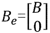
- Q f A e + A e T Q f ⁇ Q f B e R ⁇ 1 B e T Q f + Q 0
- the present applicant has found that the first weighting coefficient Qf, the second weighting coefficient Q, and the third weighting coefficient R calculated in the weighting coefficient calculation step can be ideally used as the weighting coefficients of the evaluation function represented by Equations 7 and 8. Therefore, in the setting step, the first weighting coefficient Qf is set as the weighting coefficient corresponding to the terminal cost of the evaluation function, the second weighting coefficient Q is set as the weighting coefficient corresponding to the state quantity cost, and the third weighting coefficient R is set as the weighting coefficient corresponding to the control input cost.
- a user can immediately set the weighting coefficients Qf, Q, and R of the evaluation function with respect to the time response of the plant 103 expected by the model prediction control, and therefore, can alleviate the load related to a parameter setting operation of the user.
- the model prediction control unit 102 performs model prediction control through such parameter setting, an integration amount serving as a driving source of servo control is adjusted ideally in the servo control for tracking using the model prediction control, and it is possible to realize servo control suppressing an overshoot without using a disturbance observer which requires difficult adjustment such as expansion of a disturbance model or design of an observer gain as in the conventional technique.
- Fig. 2 is a diagram illustrating an overall configuration of a control system according to a first configuration example.
- the control system includes a network 1, a servo driver 4, and a standard PLC (Programmable Logic Controller) 5.
- the servo driver 4 is a control device that executes model prediction control for servo-controlling an actual plant (hereinafter simply referred to as an "actual plant") 6 including a motor 2 and a load device 3.
- the servo driver 4 performs servo control involving model prediction control with respect to the actual plant 6 so that the output of the actual plant 6 tracks a target command transmitted from the standard PLC 5.
- the servo driver 4 With this model prediction control, the servo driver 4 generates a control input for performing servo control of the actual plant 6 on the basis of the target command received from the standard PLC 5. Generation of the control input by the servo driver 4 will be described later.
- the load device 3 that constitutes the plant 6 include various machine apparatuses (for example, an industrial robot arm and a conveying apparatus), and the motor 2 is incorporated in the load device 3 as an actuator that drives the load device 3.
- the motor 2 is an AC servo motor.
- An encoder (not illustrated) is attached to the motor 2, and a parameter signal (a position signal, a velocity signal, and the like) related to an operation of the motor 2 is transmitted to the servo driver 4 as a feedback signal by the encoder.
- the standard PLC 5 generates a target command related to an operation (motion) of the plant 6 and transmits the same to the servo driver 4.
- the servo driver 4 receives the target command from the standard PLC 5 via the network 1 and receives the feedback signal output from the encoder connected to the motor 2.
- the servo driver 4 supplies a driving current to the motor 2 so that the output of the plant 6 tracks the target command.
- the supplied current is an AC power delivered from an AC power supply to the servo driver 4.
- the servo driver 4 is a type that receives a three-phase AC power but may be a type that receives a single-phase AC power.
- the servo driver 4 has a control structure illustrated in Fig. 3 in order to realize the servo control of the actual plant 6.
- the target command supplied from the standard PLC 5 to the servo driver 4 is referred to as r.
- the servo driver 4 includes a first integrator 41, a state acquisition unit 42, and a model prediction control unit 43. The processes performed by the first integrator 41, the state acquisition unit 42, and the model prediction control unit 43 are computed and executed by an arithmetic processing device mounted in the servo driver 4.
- an offset e (e - r - y) between the target command r transmitted from the standard PLC 5 and the output y of the actual plant 6 fed back by a feedback system is input to the first integrator 41.
- the output z of the first integrator 41 is input to the model prediction control unit 43 through the state acquisition unit 42.
- the state acquisition unit 42 acquires a state variable x including the state related to the actual plant 6 and the output z of the first integrator 41, provided to the model prediction control performed by the model prediction control unit 43.
- the state acquisition unit 42 can acquire predetermined information generated from an output signal of the encoder connected to the motor 2 included in the actual plant 6 as the state variable included in the state x.
- a predetermined parameter for example, the position of an output unit of the load device 3 related to the load device 3 included in the actual plant 6 may be acquired as the state variable x.
- the state acquisition unit 42 also acquires the output z of the first integrator 41 as the state variable included in the state x.
- the model prediction control unit 43 executes model prediction control (Receding Horizon control) using the state variable x acquired by the state acquisition unit 42 and a control input u to the actual plant 6 input by the model prediction control unit 43.
- a virtual control configuration to which the control input u is input and which includes at least the actual plant 6 is formed as an expanded plant 60.
- the expression "expanded” as used herein means that the actual plant 6 solely or a combination with the actual plant 6 is regarded as a virtual control target.
- the expanded plant 60 is also referred to as an "expanded plant 60".
- a control configuration other than the actual plant 6 is not included in the expanded plant 60 and the expanded plant 60 and the actual plant 6 are identical.
- Fig. 6 to be described later illustrates an example in which the actual plant 6 and a second integrator 6a are included in the expanded plant 60.
- the output of the expanded plant 60 is identical to the output of the actual plant 6.
- Equation 14 Predetermined physical characteristics of the actual plant 6 are applied to Equation 14.
- a subscript "1" in Equation 14 indicates the number of control axes controlled by the servo driver 4, and in the present embodiment, since the number of control axes is 1, the subscripts of the respective variables of the prediction model illustrated in Equation 14 are "1".
- a state variable x 1 indicates an output position of the actual plant 6 and is a parameter fed back as the output y of the actual plant 6.
- the predetermined integral gain K i1 of the integral term included in the prediction model illustrated in Equation 14 may be adjusted on the basis of the offset e. Specifically, the predetermined integral gain K i1 is adjusted so that the value of the predetermined integral gain K i1 increases as the magnitude of the offset e decreases.
- the transition of the predetermined integral gain K i1 may be set so that the predetermined integral gain K i1 is 0 when the magnitude of the offset e is equal to or larger than a predetermined threshold, the value of the predetermined integral gain K i1 approaches abruptly 1 as the magnitude of the offset e approaches 0 when the magnitude of the offset e is smaller than the predetermined threshold, and the predetermined integral gain K i1 is 1 which is the largest value when the magnitude of the offset e is 0.
- the predetermined integral gain K i1 can be adjusted on the basis of the magnitude of the offset e, when an output y(x 1 ) of the expanded plant 60 (the actual plant 6) deviates far from a command x f1 , the value of the predetermined integral gain K i1 is adjusted to be small, and an integration amount for servo control is adjusted so as not to accumulate. Moreover, since the value of the predetermined integral gain K i1 is adjusted to be large when the amount of deviation of the output y(x 1 ) of the expanded plant 60 (the actual plant 6) from the command x f1 decreases (that is, the magnitude of the offset e decreases), it is possible to effectively enhance the trackability of servo control. By varying the value of the predetermined integral gain K i1 in this manner, it is possible to achieve both suppression of an overshoot and improvement in the trackability of servo control.
- data related to correlation between the offset e and the predetermined integral gain K i1 may be stored in the memory of the servo driver 4, and in that case, the predetermined integral gain K i1 is adjusted by accessing the data.
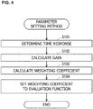
- Fig. 4 is a diagram illustrating the flow of a parameter setting method, and this method includes a time response determining step, a gain calculation step, a weighting coefficient calculation step, and a setting step.
- a time response determining step performed in S101 will be described.
- a desired time response of the optimal servo structure illustrated in Fig. 1B (that is, a time response that is expected to be realized in the control structure illustrated in Fig. 1A ) is determined.
- a relative order di and a non-interference matrix D of the optimal servo structure are calculated according to Equation 15 below.
- D c 1 A d 1 ⁇ 1 B ⁇ c m A d m ⁇ 1 B
- d i : min k : c i A k ⁇ 1 B ⁇ 0 1 ⁇ i ⁇ m
- a stabilization polynomial ⁇ i(s) of order di having a root of a pole si defined as a reciprocal of a time constant Ti based on the desired time response of the optimal servo structure is set according to Equation 16 below.
- the above-described process is performed on the basis of the time response in the optimal servo structure set by taking the time response expected to be realized in the control structure illustrated in Fig. 1A into consideration.
- the first reference optimal gain K F 0 and the second reference optimal gain K I 0 of the integration-type ILQ servo control structure (see Fig. 1C ) obtained by reconstructing the optimal servo structure according to the reconstruction method are calculated on the basis of Equation 18 below.
- Equation 19 a matrix ⁇ of the adjustment parameter is determined according to the following procedures.
- the matrix V of the adjustment parameter is a unit matrix I as a non-interference matrix.
- K F K I V ⁇ 1 ⁇ V K F 0 K I 0 ( ⁇ determination procedure)
- Equation 20 A maximum eigenvalue ⁇ max of a symmetric matrix KB+(KB) T is obtained, and the range of values ⁇ i that constitute the matrix ⁇ is determined as Equation 20 below. [Math. 18] ⁇ ⁇ ⁇ a ⁇ ⁇ > 0
- ⁇ > ⁇ max KB + KB T where ⁇ diag ⁇ 1 , ⁇ , ⁇ m
- the weighting coefficient calculation step performed in S103 will be described.
- the weighting coefficients of the evaluation function (see Equations 6 to 8) for model prediction control are calculated on the basis of a predetermined Riccati equation of an expanded offset system. Specifically, the weighting coefficients are calculated according to Procedures 6 to 9 below.
- V I
- R V ⁇ 1 ⁇ ⁇ 1
- V ⁇ ⁇ 1
- ⁇ diag ⁇ 1 , ... , ⁇ m
- Equation 26 Matrices ⁇ and Y satisfying Equation 26 below are calculated.
- the value is used as the value of the matrix ⁇ in Procedure 7 as it is.
- the matrix ⁇ does not satisfy Equation 26, the values ⁇ i constituting the matrix ⁇ are increased.
- E ⁇ ⁇ K V B V ⁇ K V B V T > 0 YF + F T Y + YGG T Y + H T H ⁇ 0
- F A K + GH , Re ⁇ F ⁇ 0
- H E ⁇ 1 / 2 K V A K
- Equation 29 a matrix Q is calculated as Equation 29 below.
- Q Q f B e R ⁇ 1 B e T Q f ⁇ Q f A e ⁇ A e T Q f
- the setting step performed in S104 will be described.
- the matrix Qf calculated according to Equation 28 is set as the weighting coefficient Qf (see Equation 7) corresponding to the terminal cost.
- the matrix Q calculated according to Equation 29 is set as the weighting coefficient Q corresponding to the state quantity cost, and the matrix R illustrated in Equation 24 is set as the weighting coefficient R corresponding to the control input cost (see Equation 8).
- a user can set the weighting coefficients Qf, Q, and R of the evaluation function for model prediction control immediately with respect to the time response of the actual plant 6 expected by the model prediction control and therefore can alleviate the load related to a parameter setting operation of the user. Since the model prediction control is performed through such parameter setting, an integration amount serving as a driving source of servo control which uses the model prediction control is adjusted ideally, and servo control which suppresses an overshoot can be realized.
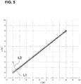
- Fig. 5 illustrates a simulation result when the control structure illustrated in Fig.
- FIG. 1A is constructed with respect to the control axes of the actual plant 6 having a plurality of control axes through the parameter setting method and model prediction control is executed on the respective control axes.
- Fig. 5 in a working coordinate system in which an output of a first control axis is set as the horizontal axis, an output of a second control axis is set as the vertical axis, the trajectory of a target command is represented by line L1 and the trajectory of the output of the actual plant 6 is represented by line L2.
- the output of the actual plant 6 ideally tracks the target command.
- the solution Qf of the Riccati equation is calculated, and the calculated Qf is set as the weighting coefficient corresponding to the terminal cost.
- the solution Qf may not be calculated in the parameter setting method.
- a coefficient calculated by a known technique may be employed as the weighting coefficient corresponding to the terminal cost.
- Servo control by the servo driver 4 according to a second configuration example will be described with reference to Fig. 6 .
- the expanded plant 60 including the actual plant 6 is formed similarly to the first configuration example, model prediction control is performed by the model prediction control unit 43, and the output z of the first integrator 41 is acquired by the state acquisition unit 42 and is provided to the model prediction control.
- the second integrator 6a and the actual plant 6 are combined to form the expanded plant 60 as illustrated in the lower part (b) of Fig. 6 .
- the control input u is a jerk input (d ⁇ /dt).
- the prediction model of the model prediction control unit 43 can be represented by Equation 31 below.
- Equation 31 a correlation between the expanded state variable and the jerk input u which is a control input is defined.
- the model prediction control unit 43 generates the jerk input u which is a control input on a real-time basis and outputs the jerk input u to the expanded plant 60.
- the evaluation function (see Equations 6 to 8) for model prediction control to which the weighting coefficients are set by the parameter setting method illustrated in Fig. 4 is used.
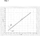
- Fig. 7 illustrates a simulation result when the control structure illustrated in Fig. 1A is constructed with respect to the control axes of the actual plant 6 having a plurality of control axes through the parameter setting method and model prediction control is executed on the respective control axes.
- Servo control by the servo driver 4 according to a third configuration example will be described with reference to Fig. 8 .
- the expanded plant 60 including the actual plant 6 is formed similarly to the second configuration example, a filter unit 7 is incorporated into the expanded plant 60 to form a further expanded plant 600, and model prediction control is performed by the model prediction control unit 43.
- a difference between a target command and the output of the further expanded plant 600 (that is, the output of the actual plant 6) is supplied to a servo integrator 41, and the output z of the servo integrator 41 and the expanded state variable of the further expanded plant 600 are acquired by the state acquisition unit 42 and are provided to the model prediction control.
- the filter unit 7 performs an attenuation process at a predetermined frequency with respect to the signal (in the present embodiment, the control input u (jerk input) to the further expanded plant 600) input to the filter unit 7.
- the predetermined frequency is preferably the frequency of vibration related to the actual plant 6 which is a direct vibration suppression target during servo control.
- the resonant frequency of the actual plant 6 can be set as the predetermined frequency.
- the attenuation process is a process of attenuating the gain of the signal (control input) related to the predetermined frequency to a desired extent.
- the filter unit 7 may be configured as a notch filter in which the predetermined frequency is set as a central frequency of the attenuation process, or may be configured as a low-pass filter in which the predetermined frequency is set as a cutoff frequency of the attenuation process.
- the filter unit 7 is formed in this manner, the signal (the control input u) on which an attenuation process has been performed by the filter unit 7 is input to the expanded plant 60 including the actual plant 6.
- suppression of vibration in the actual plant 6 is expected during servo control of the actual plant 6, and the output of the actual plant 6 can approach a target in a desired period.
- the prediction model of the model prediction control unit 43 is determined.
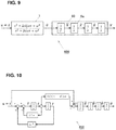
- Fig. 9 illustrates a transfer function of the filter unit 7 and a transfer function of the expanded plant 60.
- An output when the control input u is input to the filter unit 7 is represented by dv/dt, and the output dv/dt is set as an input to the expanded plant 60.
- a jerk input is set as the control input u of the present embodiment.
- Fig. 10 illustrates a control structure of the further expanded plant 600 in which the transfer function of the filter unit 7 and the transfer function of the expanded plant 60 are taken into consideration.
- the prediction model of the model prediction control unit 43 can be represented by Equation 33 below.
- x x 1 x ⁇ 1 x ⁇ 1 z 1 ⁇ 1 ⁇ ⁇ 1
- P x ⁇ 1 x ⁇ 1 u 1 J 1 x f 1 ⁇ x 1 k i 1 ⁇ ⁇ 1 ⁇ ⁇ 1 2 ⁇ 1 ⁇ 2 ⁇ 1 ⁇ 1 + u 1
- the model prediction control unit 43 generates the jerk input u which is a control input on a real-time basis and outputs the jerk input u to the filter unit 7 included in the further expanded plant 600.
- the prediction model (a prediction model represented by Equation 33) of this configuration example is compared with the prediction model (a prediction model represented by Equation 31) of the second configuration example, it is understood that the order of the prediction model of this configuration example is larger than that of the second configuration example by an amount corresponding to the state variable related to the filter unit 7.
- the state variable related to the filter unit 7 has a correlation with evaluation (that is, evaluation of optimality based on an evaluation function) of optimality of model prediction control.
- evaluation that is, evaluation of optimality based on an evaluation function
- a weighting coefficient corresponding to the state quantity cost is generated using the weighting coefficient obtained in the second configuration example.
- the weighting coefficients Qf, Q, and R of the evaluation function are calculated according to a prediction model that does not include the state variable of the filter unit 7 (that is, the prediction model of the second configuration example (the prediction model represented by Equation 31)). Since the weighting coefficient Q related to the state quantity cost among these weighting coefficients corresponds to the expanded plant 60 at this time point, the dimension thereof is different from the dimension of the expanded state variable of the further expanded plant 600.
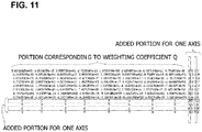
- Fig. 11 illustrates an example of the weighting coefficient Q' related to the state quantity cost.
- the weighting coefficient Q' in Fig. 11 and the weighting coefficient Q which is the base thereof correspond to model prediction control in which the number of control axes is two.
- the prediction model (a prediction model represented by Equation 33) of this configuration example includes a larger number of state variables than that of the prediction model (the prediction model represented by Equation 31) of the second configuration example by the number (two) of state variables related to the filter unit 7. Therefore, zeros are added to the weighting coefficient Q by an amount corresponding to the number of dimensions corresponding to this difference to generate a new weighting coefficient Q', which is illustrated in Fig. 11 .
- the weighting coefficient Q' illustrated in Fig. 11 corresponds to model prediction control in which the number of control axes is two
- zeros are added by an amount corresponding to the difference in the number of dimensions corresponding to two control axes.
- the first weighting coefficient Qf (the weighting coefficient Qf calculated according to the prediction model of the second configuration example) is set as the weighting coefficient corresponding to the terminal cost
- the new second weighting coefficient Q' is set as the weighting coefficient corresponding to the state quantity cost
- the third weighting coefficient R (the weighting coefficient R calculated according to the prediction model of the second configuration example) is set as the weighting coefficient corresponding to the control input cost.
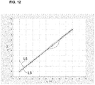
- Fig. 12 illustrates a simulation result when the control structure illustrated in Fig. 1A is constructed with respect to the control axes of the actual plant 6 having a plurality of control axes through the parameter setting method and model prediction control is executed on the respective control axes.
- a control structure which is formed in the standard PLC 5 and includes a model prediction control unit 53 corresponding to the model prediction control unit 43 will be described with reference to Fig. 13 .
- the standard PLC 5 includes a command generation unit 50, an integrator 51, a state acquisition unit 52, a model prediction control unit 53, and an expanded plant model 560. Since the integrator 51, the state acquisition unit 52, and the model prediction control unit 53 substantially correspond to the integrator 41, the state acquisition unit 42, and the model prediction control unit 43 illustrated in Figs. 3 , 6 , and 8 , respectively, the detailed description thereof will be omitted.
- the command generation unit 50 generates a target command r for instructing the output of the actual plant 6.
- the target command r is provided to model prediction control of the model prediction control unit 53 rather than being supplied from the standard PLC 5 directly to the servo driver 4.
- the expanded plant model 560 has an expansion system model including a plant model that models the expanded plant 60 illustrated in Figs. 3 and 6 or the further expanded plant 600 illustrated in Fig. 8 and simulates the output of the expanded plant 60 or the like using the expansion system model.
- the simulation result is used as an output y of the expanded plant model 560.
- the output y of the expanded plant model 560 is fed back to an input side of the integrator 51 by a feedback system.
- An output z of the integrator 51 is input to the model prediction control unit 53 through the state acquisition unit 52.
- the state acquisition unit 52 acquires the value of a state variable included in the state x related to the expansion system model, provided to the model prediction control performed by the model prediction control unit 53.
- the acquisition of the state variable by the state acquisition unit 52 is substantially the same as acquisition of the state variable by the state acquisition unit 42 illustrated in the first to third configuration examples described above.
- the model prediction control unit 53 executes model prediction control using the state x acquired by the state acquisition unit 52 and the input u to the expanded plant model 560 output by the model prediction control unit 53.
- an integral term represented by a product of the offset e and the predetermined integral gain is included in the prediction model used in the model prediction control substantially similarly to the model prediction control performed by the model prediction control unit 43 illustrated in the first to third configuration examples described above.
- the standard PLC 5 illustrated in Fig. 13 can supply the output y which is the simulation result of the expanded plant model 560 to the servo driver 4 as a command for ideally tracking the target command r while suppressing the output of the actual plant 6 from entering an overshoot state. That is, the standard PLC 5 can suppress occurrence of a steady-state offset in the output of the actual plant 6 while performing model prediction control even when the target trajectory changes frequently according to the target command r although the control amount of the actual plant 6 which is the actual control target is not fed back directly.
- the parameter setting method illustrated in Fig. 4 can be applied to the setting of the weighting coefficients of the evaluation function in the model prediction control.
- model prediction control is performed in the standard PLC 5 through such parameter setting, an integration amount serving as a driving source of servo control is adjusted ideally in the servo control for tracking using the model prediction control, it is possible to realize servo control suppressing an overshoot.
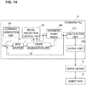
- a fifth configuration example relates to a modification of the standard PLC 5 having a control structure including the model prediction control unit 53 similarly to the fourth configuration example and will be described with reference to Figs. 14 and 15 .
- Fig. 14 illustrates a control structure of the standard PLC 5 according to this configuration example, and functional units substantially the same as those of the standard PLC 5 of the fourth configuration example will be denoted by the same reference numerals, and the detailed description thereof will be omitted.
- the plant 6 is a robot arm 6 illustrated in Fig. 15A . Therefore, the expanded plant model 560 has an expansion system model to which the structure of the robot arm 6 is applied and performs simulation of the expanded plant model 60 using the expansion system model.
- the robot arm 6 which is a plant will be described with reference to Fig. 15A .
- the robot arm 6 has two motors 2 (motors 2a and 2b) driven according to a target command from the standard PLC 5.
- one end of a first arm 3a is attached to an output shaft of the motor 2a so that the first arm 3a is rotated using the motor 2a as a first joint.
- a motor 2b is disposed at the other end of the first arm 3a, and one end of a second arm 3b is attached to an output shaft of the motor 2b so that the second arm 3b is rotated using the motor 2b as a second joint.
- a tip 3c of the second arm 3b is an output unit of the robot arm 6, and an end effector for grasping a predetermined object, for example, is attached to the tip 3c.
- a plane of rotation of the first arm 3a is the same plane as a plane of rotation of the second arm 3b, and an x1-axis and an x2-axis are set as orthogonal coordinates for defining the plane of rotation.
- This orthogonal coordinates are working coordinates related to the robot arm 6, and the position of the tip 3c of the robot arm 6 can be defined on the orthogonal coordinates.
- the command generation unit 50 of this configuration example generates a predetermined command r that the tip 3c of the robot arm 6 has to track. This command r is based on the working coordinate system (see Figs. 15A and 15B ) related to the robot arm 6.
- An output y of the expanded plant model 560 obtained when the control input u is input is based on the working coordinate system illustrated in Figs. 15A and 15B .
- the motors 2a and 2b that form the robot arm 6 are actuators that are rotated, and a rotation coordinate system which is an independent coordinate system different from the working coordinate system is set to the respective motors for servo control performed by the servo driver 4. Therefore, the output y is not used as a target command for driving the motors 2a and 2b as it is. Therefore, the calculation unit 570 performs a calculation process for converting the output y of the expanded plant model 560 to a target command based on the rotation coordinate system of the motors.
- Fig. 15B illustrates the apparatus structure of the robot arm 6.
- the first joint at which the motor 2a is disposed is positioned at the origin of the working coordinate system in order to simplify the description.
- the rotation angles ⁇ 1 and ⁇ 2 of the motors 2a and 2b can be represented by Equation 34 below when the geometric relation of the apparatus structure of the robot arm 6 is taken into consideration.
- the rotation angle ⁇ 1 of the motor 2a is defined as the angle between the x1-axis and the first arm 3a
- the rotation angle ⁇ 2 of the motor 2b is defined as the angle between the first arm 3a and the second arm 3b.
- ⁇ 2 atan 2 ⁇ 2 L 1 L 2 2 ⁇ L 0 2 ⁇ L 1 2 + L 2 2 2 2 L 1 L 2 L 0 2 ⁇ L 1 2 + L 2 2 2 L 1 L 2
- a function atan2 in Equation 34 is a function that returns a drift angle of (x, y) in the coordinate system when represented by atan2(x, y).
- the angles ⁇ 1 and ⁇ 2 calculated from the output y of the expanded plant model 560 by the calculation unit 570 in this manner are the target commands related to the positions (angles) of the motors, ideal for servo-controlling the motors 2a and 2b. Therefore, the calculation result obtained by the calculation unit 570 is supplied to the servo driver 4 by a supply unit 580 and is provided to servo control (feedback control) in the servo driver 4.
- the model prediction control performed in the standard PLC 5 is performed on the basis of the working coordinate system related to the robot arm 6. Therefore, it is easy to allow the output of the robot arm 6 to ideally track a predetermined command r based on the working coordinate system.
- the result of the model prediction control based on the working coordinate system can be converted to a target command which can be ideally applied to the servo control of the motors 2a and 2b based on the rotation coordinate system.
- the calculation process is based on the geometric relation of the apparatus structure of the robot arm 6, it is possible to ideally avoid occurrence of an output error (position error) of the robot arm 6 resulting from accumulation of computation errors. This is very useful effect in considering the trackability of the robot arm 6.
- the parameter setting method illustrated in Fig. 4 can be applied to the setting of the weighting coefficients of the evaluation function in the model prediction control.
- the prediction model of the model prediction control unit 53 in the standard PLC 5 is based on the working coordinate system which is an orthogonal coordinate system, it is possible to immediately set the weighting coefficients Qf, Q, and R of the evaluation function according to the parameter setting method and ideally alleviate the load related to the setting.
- model prediction control is performed in the standard PLC 5 through such parameter setting, an integration amount serving as a driving source of servo control is adjusted ideally in the servo control for tracking using the model prediction control, it is possible to realize servo control suppressing an overshoot.
- the control structure for servo control illustrated in the first to third configuration examples is preferably formed in the standard PLC 5 as illustrated in the fourth and fifth configuration examples.
- the control structure for servo control illustrated in the first to third configuration examples is preferably formed in the standard PLC 5 as illustrated in the fourth and fifth configuration examples.
Landscapes
- Engineering & Computer Science (AREA)
- Automation & Control Theory (AREA)
- Physics & Mathematics (AREA)
- General Physics & Mathematics (AREA)
- Computer Vision & Pattern Recognition (AREA)
- Medical Informatics (AREA)
- Software Systems (AREA)
- Evolutionary Computation (AREA)
- Health & Medical Sciences (AREA)
- Artificial Intelligence (AREA)
- Robotics (AREA)
- Mechanical Engineering (AREA)
- Human Computer Interaction (AREA)
- Manufacturing & Machinery (AREA)
- Feedback Control In General (AREA)
Abstract
Description
- The present invention relates to a method for setting control parameters for model prediction control.
- Generally, feedback control is used in order to control a control target to track a command trajectory. For example, a control device of an articulated robot controls servo motors of respective joint shafts using feedback control so that the position of a hand of the robot tracks a command trajectory set (taught) in advance. However, general feedback control has a problem that since a response delay occurs inevitably in each servo motor, the actual trajectory of the robot deviates from the command trajectory. Techniques related to model prediction control are used to suppress such a deviation from the command trajectory.
- However, even when model prediction control is used, a steady-state offset may occur if a target trajectory for a command changes frequently as in tracking control. Therefore, when a servo system is constructed using model prediction control, the steady-state offset may be eliminated by connecting an integrator to a compensator thereof in series. Moreover, the steady-state offset can be removed in principle by incorporating an assumed disturbance into the model by regarding the disturbance as a new state. For example, NPL 1 and NPL 2 propose methods for constructing a disturbance observer and cancelling a steady-state offset using a disturbance estimated by the disturbance observer.
-
- NPL 1: Yuta Sakurai and Toshiyuki Ohtsuka: Offset Compensation of Continuous Time Model Predictive Control By Disturbance Estimation; Journal of Institute of Systems, Control and Information Engineers, Vol. 25, No. 7, pp. 10-18 (2012)
- NPL 2: U. Maeder and M. Morari: Linear offset-free model predictive control; Automatica, Vol. 45, No. 10, pp. 2214-2222 (2009)
- NPL3: Fatima TAHIR and Toshiyuki OHTSUKA: Tuning of Performance Index in Nonlinear Model Predictive Control by the Inverse Linear Quadratic Regulator Design Method, SICE Journal of Control, Measurement, and System Integration, Vol. 6, No. 6, pp. 387-395, (2013)
- When model prediction control is performed for servo control in which an output of a control target is controlled to track a target command, an optimal control input is calculated according to a predetermined evaluation function. Generally, in the predetermined evaluation function, a terminal cost related to a state variable of the control target and a stage cost related to the state variable and the control input are calculated, and the control input is optimized so that the sum thereof is immunized. In this case, the weighting coefficients of the terminal cost and the stage cost are set in the evaluation function whereby the control input is optimized in a state in which a correlation of the costs is applied.
- Here, the weighting coefficients of the model prediction control cannot easily find an immediate relationship with a time response of the control target of the model prediction control. Therefore, a user requires numerous trial-and-errors in determining the weighting coefficients for model prediction control. Although NPL 3 discloses a method for determining weighting coefficients for model prediction control by taking a time response of a control target into consideration when a regulator performs model prediction control, this method cannot deal with servo control.
- The present invention has been made in view of the above-described problems, and an object thereof is to provide a technique for allowing a user to set weighting coefficients for model prediction control immediately on the basis of a time response of a control target when model prediction control is performed for servo control in which an output of a control target is controlled to track a target command.
- In the present invention, in order to solve the problems, it is assumed that a system that linearizes a prediction model used in model prediction control near a terminal end and an optimum servo control structure corresponding to a control structure that performs servo control using the model prediction control output the same output with respect to the same control input. In this way, when model prediction control is performed for servo control using so-called an ILQ design method, a user can set weighting coefficients immediately on the basis of a time response of a control target.
- Specifically, the present invention provides a method for setting control parameters for model prediction control (hereinafter, also referred to simply as a "control parameter setting method") related to a predetermined control target, the method being executed by a control device having a first integrator to which an offset between a predetermined target command and an output of the predetermined control target corresponding to an actual target device which is an actual target of servo control is input, in order to allow an output of the actual target device tracks the predetermined target command. The control device includes a model prediction control unit which has a prediction model that defines a correlation between a predetermined expanded state variable related to an expanded control target including at least the predetermined control target and a control input to the expanded control target in a form of a predetermined state equation and which performs the model prediction control based on the prediction model according to a predetermined evaluation function in a prediction section having a predetermined time width with respect to the predetermined target command and outputs a value of the control input at least at an initial time point of the prediction section. Moreover, a predetermined state variable which is a portion of the predetermined expanded state variable and is related to the predetermined control target includes a predetermined integral term represented by a product of the offset and a predetermined integral gain.
- The setting method includes: a time response determining step of determining a desired time response in an optimum servo control structure which includes a virtual integrator virtually corresponding to the first integrator and is related to a virtual control target virtually corresponding to the expanded control target and in which, when a virtual target command for the virtual control target is r1, a virtual control input to the virtual control target is a virtual control input u1, and a virtual output of the virtual control target is y1, the virtual control input u1 is represented by
Equation 1 below including a state feedback gain KF and an integral gain KI; a gain calculation step of calculating the state feedback gain KF and the integral gain KI corresponding to the desired time response; a weighting coefficient calculation step of calculating a second weighting coefficient Q and a third weighting coefficient R among a first weighting coefficient Qf, the second weighting coefficient Q, and the third weighting coefficient R in a predetermined Riccati equation represented byEquation 3 below on the basis of the state feedback gain KF and the integral gain KI when the control input to the expanded control target is u, the output of the expanded control target is y, the offset is e, the predetermined state variable is x, and a state equation related to the predetermined control target is represented byEquation 2 below; and a setting step of setting the second weighting coefficient Q as a weighting coefficient corresponding to a state quantity cost which is a stage cost related to the predetermined state variable and setting the third weighting coefficient R as a weighting coefficient corresponding to a control input cost which is a stage cost related to the control input in the predetermined evaluation function. - Furthermore, in the weighting coefficient calculation step, the first weighting coefficient Qf may be further calculated. In this case, in the setting step, the first weighting coefficient Qf may be set as the weighting coefficient corresponding to the terminal cost related to the predetermined state variable.
[Math. 1]


- In the control parameter setting method of the present disclosure, weighting coefficients for model prediction control used for allowing a final output of an actual target device to track a predetermined target command are calculated by determining a time response of an output of a virtual control target (that is, a time response of an output of an expanded control target) in the optimum servo control structure according to
Equation 1. That is, by using the control parameter setting method, a user can easily acquire weighting coefficients for model prediction control corresponding to the time response recognizable immediately and does not need to repeat trial-and-errors related to weighting coefficients for model prediction control for tracking a target command unlike the conventional technique. The predetermined control target may be an actual target device and may be an actual target model that models the actual target device. When the predetermined control target is an actual target model, the expanded control target is an expansion system model including the actual target model. - In the control parameter setting method, the expanded control target may include the predetermined control target only, and a portion of the predetermined expanded state variable may be identical to the predetermined state variable. The control parameter setting method according to the present disclosure can be applied to a form in which the expanded control target is identical to the predetermined control target, and therefore, a user does not need to repeat trial-and-errors related to weighting coefficients for model prediction control.
- As another method, in the control parameter setting method, the control input may be a jerk input to the predetermined control target, and the expanded control target may include additional integrator that performs a predetermined integration process with respect to the jerk input in addition to the predetermined control target. In this case, the prediction model may define a correlation between the jerk input and the predetermined expanded state variable including the predetermined state variable related to the predetermined control target and a state variable related to the additional integrator. The control parameter setting method according to the present disclosure can be applied to a form in which the expanded control target includes additional integrator for the jerk input together with the predetermined control target, and therefore, a user does not need to repeat trial-and-errors related to weighting coefficients for model prediction control.
- Furthermore, a filter unit that performs an attenuation process at a predetermined frequency with respect to a control input based on the predetermined target command may be included in the predetermined control target and the expanded control target including the additional integrator whereby a further expanded control target is formed in the control device, and the control parameter setting method according to the present disclosure may be the control parameter setting method for the model prediction control executed by the control device. In this case, a state variable related to the further expanded control target may include a state variable related to the filter unit in addition to the predetermined expanded state variable, and the prediction model may define a correlation between the jerk input and the predetermined expanded state variable and the state variable related to the filter unit. In the weighting coefficient calculation step, the second weighting coefficient Q and the third weighting coefficient R may be calculated on the basis of the state feedback gain KF and the integral gain KI, and zeros may be added to the second weighting coefficient as a weighting coefficient corresponding to the state variable related to the filter unit so as to correspond to the further expanded control target to obtain a new second weighting coefficient. In the setting step, the new second weighting coefficient may be set as the weighting coefficient corresponding to the state quantity cost and the third weighting coefficient R may be set as the weighting coefficient corresponding to the control input cost in the predetermined evaluation function.
- Furthermore, in the weighting coefficient calculation step, the first weighting coefficient Qf, the second weighting coefficient Q, and the third weighting coefficient R corresponding to the expanded control target may be calculated on the basis of the state feedback gain KF and the integral gain KI. In this case, in the setting step, the first weighting coefficient Qf may be further set as the weighting coefficient corresponding to the terminal cost in the predetermined evaluation function.
- In these cases, the further expanded control target includes a filter unit in addition to the predetermined control target and the additional integrator, and a state variable related to the filter unit is applied to the prediction model for the model prediction control. In this way, with the model prediction control, it is possible to realize ideal tracking of the target command while suppressing vibration of the output of the predetermined control target. Here, the attenuation process itself by the filter unit is not to be substantially applied to optimization of the control input according to the predetermined evaluation function. Therefore, in the weighting coefficient calculation step, zeros may be added to the second weighting coefficient calculated for the expanded control target including the predetermined control target and the additional integrator as a weighting coefficient corresponding to the state variable related to the filter unit to obtain a new second weighting coefficient, which can be employed as a final weighting coefficient for the model prediction control. In this way, it is possible to eliminate user's trial-and-errors related to weighting coefficients for model prediction control.
- The filter unit may be configured as a notch filter in which the predetermined frequency is used as a central frequency of the attenuation process or a low-pass filter in which the predetermined frequency is used as a cutoff frequency of the attenuation process. Moreover, the filter unit may be configured as a filter other than these filters.
- A user can set weighting coefficients for model prediction control immediately on the basis of a time response of a control target when model prediction control is performed for servo control in which an output of a control target is controlled to track a target command.
-
- [
Fig. 1A] Fig. 1A is a diagram illustrating an example of a control structure to which a method for setting control parameters for model prediction control is applied. - [
Fig. 1B] Fig. 1B is a diagram illustrating an optimal servo structure corresponding to the control structure illustrated inFig. 1A . - [
Fig. 1C] Fig. 1C is an integration-type ILQ servo control structure obtained by reconstructing the optimal servo structure illustrated inFig. 1B . - [
Fig. 2] Fig. 2 is a diagram illustrating a control structure of a servo driver according to a first configuration example. - [
Fig. 3] Fig. 3 is a diagram illustrating a control structure of a servo driver according to the first configuration example. - [
Fig. 4] Fig. 4 is a diagram illustrating the flow of a method for setting weighting coefficients (control parameters) of an evaluation function for model prediction control executed in the servo driver according to the first configuration example. - [
Fig. 5] Fig. 5 is a diagram illustrating the result of trackability when an actual plant having two control axes is servo-controlled by the servo driver according to the first configuration example. - [
Fig. 6] Fig. 6 is a diagram illustrating a control structure of a servo driver according to a second configuration example. - [
Fig. 7] Fig. 7 is a diagram illustrating the result of trackability when an actual plant having two control axes is servo-controlled by the servo driver according to the second configuration example. - [
Fig. 8] Fig. 8 is a diagram illustrating a control structure of a servo driver according to a third configuration example. - [
Fig. 9] Fig. 9 is a diagram illustrating a transfer function related to a further expanded plant in the servo driver according to the third configuration example. - [
Fig. 10] Fig. 10 is a diagram illustrating a detailed control structure related to a further expanded plant. - [
Fig. 11] Fig. 11 is a diagram illustrating an example of weighting coefficients corresponding to a state quantity cost in the third configuration example. - [
Fig. 12] Fig. 12 is a diagram illustrating the result of trackability when an actual plant having two control axes is servo-controlled by the servo driver according to the third configuration example. - [
Fig. 13] Fig. 13 is a diagram illustrating a control structure of a standard PLC according to a fourth configuration example. - [
Fig. 14] Fig. 14 is a diagram illustrating a control structure of a standard PLC according to a fifth configuration example. - [
Fig. 15] Figs. 15A and 15B are diagrams illustrating an overall configuration of a robot arm which is a plant according to the fifth configuration example. - An example of a scene in which a method for setting control parameters for model prediction control according to the present invention is applied will be described with reference to
Figs. 1A to 1C .Fig. 1A illustrates a control structure that executes tracking control (servo control) for causing an output y of aplant 103 which is a control target to track a target command r. In the control structure, model prediction control is executed by the modelprediction control unit 102, whereby tracking control to the target command r is realized, a control input to theplant 103 calculated by the model prediction control is referred to as u, and a state variable related to theplant 103 used for calculation of the model prediction control is referred to as x. - In the control structure, an offset e (e = r - y) between the target command r and the output y of the
plant 103 is input to afirst integrator 101. An output z of thefirst integrator 101 is also included in the state variable x used for calculation of the model prediction control. Therefore, the modelprediction control unit 102 performs model prediction control using the state variable x related to theplant 103 and the output z of thefirst integrator 101. Moreover, the state variable x related to theplant 103 is passed through ablock 104 whereby the output y of theplant 103 is generated. Therefore, the state equation related to theactual plant 6 is represented byEquation 4 below.
[Math. 2]
- Here, model prediction control executed by the model
prediction control unit 102 will be described. The modelprediction control unit 102 executes model prediction control (Receding Horizon control) using the state variable x including the output z of thefirst integrator 101 and the control input u to theplant 103 output by the modelprediction control unit 102. The modelprediction control unit 102 has a prediction model that defines a correlation between the state variable x and the control input u by the following state equation (Equation 5).Equation 5 below is a nonlinear state equation. Predetermined physical characteristics of theplant 103, for example, may be applied to the prediction model.
[Math. 3]
- Here, the model
prediction control unit 102 performs model prediction control based on the prediction model represented byEquation 5 according to the evaluation function illustrated inEquation 6 below in a prediction section having a predetermined time width T using the state variable x and the control input u as an input.
[Math. 4]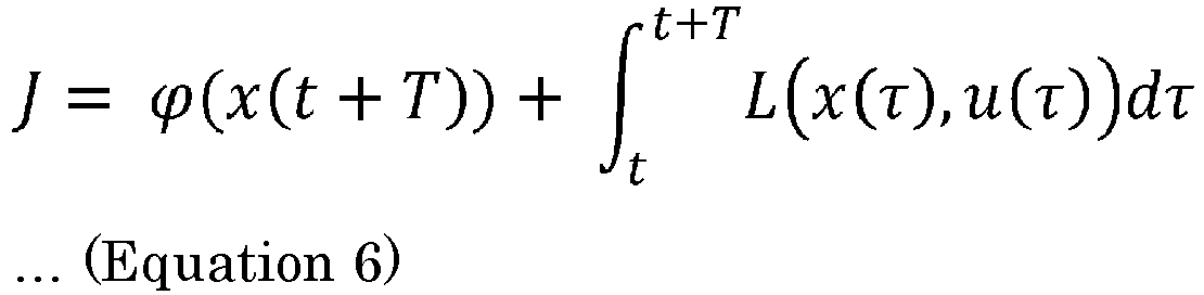
- The first term on the right side of
Equation 6 is a terminal cost, and the second terminal on the right side is a stage cost. The terminal cost can be represented byEquation 7 below, and the stage cost can be represented byEquation 8 below.
[Math. 5]

- Here, xref(k) represents a target state quantity at time point k, x(k) represents a calculated state quantity at time point k, uref(k) represents a target control input in a normal state at time point k, and u(k) represents a calculated control input at time point k. Qf in
Equation 7 is a coefficient (a weighting coefficient) indicating a weighting factor of a state quantity of the terminal cost. Moreover, Q and R inEquation 8 are a coefficient (a weighting coefficient) representing a weighting factor of a state quantity of the stage cost and a coefficient (a weighting coefficient) representing a weighting factor of a control input, respectively. Therefore, the first term on the right side ofEquation 8 means a stage cost related to a state quantity and is referred to as a "state quantity cost", and the second term on the right side means a stage cost related to a control input and is referred to as a "control input cost". - A value of the control input u at initial time point t of the prediction section, calculated in the model prediction control on the basis of the above is output as a control input u to the
plant 103 corresponding to the target command r at that time point t. In the model prediction control, a prediction section having a predetermined time width T is set at each control time point and the control input u at the control time point is calculated according to the evaluation function ofEquation 6 and is supplied to theplant 103. A problem of calculating an operation amount that optimizes a value of an evaluation function J having such a form as inEquation 6 is a problem widely known as an optimal control problem, and an algorithm for calculating a numerical solution thereof is disclosed as a known technique. A continuous deformation method can be exemplified as such a technique, and the details thereof are disclosed, for example, in "A continuation/GMRES method for fast computation of nonlinear receding horizon control", T. Ohtsuka, Automatica, Vol. 40, pp. 563-574 (2004), for example. - In a continuous deformation method, an input U(t) to model prediction control is calculated by solving a simultaneous linear equation related to the input U(t) illustrated in
Equation 9 below. Specifically,Equation 9 below is solved and dU/dt is numerically integrated to update the input U(t). In this manner, since the continuous deformation method does not perform repeated computation, it is possible to suppress a computational load for calculating the input U(t) at each time point as much as possible.
[Math. 7]
- Where F and U(t) are represented by
Equation 10 below.
[Math. 8]
- Where H is a Hamiltonian, λ is a costate, and µ is a Lagrange multiplier of constraints C=0.
- Next, a method for setting the terminal cost of the evaluation function and the weighting coefficient related to the stage cost will be described. The setting method includes a time response determining step, a gain calculation step, a weighting coefficient calculation step, and a setting step.
- Here, an optimal servo structure related to a virtual plant virtually corresponding to the
plant 103 is illustrated inFig. 1B . The optimal servo structure includes avirtual integrator 201 virtually corresponding to thefirst integrator 101, avirtual plant 203 virtually corresponding to theplant 103, and avirtual block 204 virtually corresponding to theblock 104. When a virtual target command is r1, a virtual control input to thevirtual plant 203 is a virtual control input u1, and an output of thevirtual plant 203 is y1, a virtual control input u1 is represented by Equation 11 below. Here, KF is a state feedback gain and KI is an integral gain.
[Math. 9]
- The optimal servo structure formed in this manner corresponds to a structure in which a prediction model of the control structure illustrated in
Fig. 1A is linearized near a terminal end. As a result, in the control structure ofFig. 1A and the optimal servo structure ofFig. 1B , when the variables x, z, and u which are evaluation items and the weighting coefficients Qf, Q, and R are focused on, the input/output of the optimal servo structure can be correlated with the input/output of the control structure illustrated inFig. 1A (that is, the input/output of the control structure in which model prediction control is performed by the model prediction control unit 102). Based on this fact, first, in the time response determining step, a desired time response of the optimal servo structure is determined. That is, this determination substantially means determining a time response that is expected to be realized in the control structure illustrated inFig. 1A . - Subsequently, in the gain calculation step, a state feedback gain KF and an integral gain KI of the optimal servo structure corresponding to the desired time response determined in the statistic process are calculated. Calculates of these gains are realized using a method (hereinafter referred to as a "reconstruction method") of reconstructing an optimum servo control structure illustrated in
Fig. 1B an integration-type ILQ servo control structure illustrated inFig. 1C . Components common with the optimal servo structure ofFig. 1B and the integration-type ILQ servo control structure ofFig. 1C will be denoted by the same reference numerals, and the description thereof will be omitted. A difference of the integration-type ILQ servo control structure ofFig. 1C from the optimum servo control structure ofFig. 1B is that a gainadjustment parameter block 206 common to the state feedback gain KF and the integral gain KI are tied up, and as a result, in the integration-type ILQ servo control structure, the gains are represented by a first reference optimal gain KF 0 (indicated by 205') and a second reference optimal gain KI 0 (indicated by 202') which are reference optimal gains. Moreover, the adjustment parameter of theblock 206 is represented by Equation 12 below, and ∑ in the equation is a responsiveness matrix designating a time responsiveness in a first-order lag form, and V is a non-interference matrix for simplifying computation. When the integration-type ILQ servo control structure is reconstructed by such a reconstruction method, the state feedback gain KF and the integral gain KI for realizing a time response ideally approximated in the first-order lag form to the time response determined through the determination of the adjustment parameter and the calculation of the first reference optimal gain KF 0 and the second reference optimal gain KI 0 are calculated.
[Math. 10]
- Subsequently, in the weighting coefficient calculation step, based on the fact that the state equation related to the
plant 103 is represented byEquation 4 described above, a first weighting coefficient Qf, a second weighting coefficient Q, and a third weighting coefficient R of a predetermined Riccati equation is calculated according to the Riccati equation represented by Equation 13 below on the basis of the state feedback gain KF and the integral gain KI calculated in the gain calculation step.
[Math. 11]
- The present applicant has found that the first weighting coefficient Qf, the second weighting coefficient Q, and the third weighting coefficient R calculated in the weighting coefficient calculation step can be ideally used as the weighting coefficients of the evaluation function represented by
Equations - According to such a control parameter setting method, a user can immediately set the weighting coefficients Qf, Q, and R of the evaluation function with respect to the time response of the
plant 103 expected by the model prediction control, and therefore, can alleviate the load related to a parameter setting operation of the user. When the modelprediction control unit 102 performs model prediction control through such parameter setting, an integration amount serving as a driving source of servo control is adjusted ideally in the servo control for tracking using the model prediction control, and it is possible to realize servo control suppressing an overshoot without using a disturbance observer which requires difficult adjustment such as expansion of a disturbance model or design of an observer gain as in the conventional technique. -
Fig. 2 is a diagram illustrating an overall configuration of a control system according to a first configuration example. The control system includes anetwork 1, aservo driver 4, and a standard PLC (Programmable Logic Controller) 5. Theservo driver 4 is a control device that executes model prediction control for servo-controlling an actual plant (hereinafter simply referred to as an "actual plant") 6 including amotor 2 and aload device 3. In the control system, theservo driver 4 performs servo control involving model prediction control with respect to theactual plant 6 so that the output of theactual plant 6 tracks a target command transmitted from thestandard PLC 5. With this model prediction control, theservo driver 4 generates a control input for performing servo control of theactual plant 6 on the basis of the target command received from thestandard PLC 5. Generation of the control input by theservo driver 4 will be described later. In this case, examples of theload device 3 that constitutes theplant 6 include various machine apparatuses (for example, an industrial robot arm and a conveying apparatus), and themotor 2 is incorporated in theload device 3 as an actuator that drives theload device 3. For example, themotor 2 is an AC servo motor. An encoder (not illustrated) is attached to themotor 2, and a parameter signal (a position signal, a velocity signal, and the like) related to an operation of themotor 2 is transmitted to theservo driver 4 as a feedback signal by the encoder. - The
standard PLC 5 generates a target command related to an operation (motion) of theplant 6 and transmits the same to theservo driver 4. Theservo driver 4 receives the target command from thestandard PLC 5 via thenetwork 1 and receives the feedback signal output from the encoder connected to themotor 2. Theservo driver 4 supplies a driving current to themotor 2 so that the output of theplant 6 tracks the target command. The supplied current is an AC power delivered from an AC power supply to theservo driver 4. In the present embodiment, theservo driver 4 is a type that receives a three-phase AC power but may be a type that receives a single-phase AC power. - Here, the
servo driver 4 has a control structure illustrated inFig. 3 in order to realize the servo control of theactual plant 6. The target command supplied from thestandard PLC 5 to theservo driver 4 is referred to as r. Theservo driver 4 includes afirst integrator 41, astate acquisition unit 42, and a modelprediction control unit 43. The processes performed by thefirst integrator 41, thestate acquisition unit 42, and the modelprediction control unit 43 are computed and executed by an arithmetic processing device mounted in theservo driver 4. In the control structure of theservo driver 4, an offset e (e - r - y) between the target command r transmitted from thestandard PLC 5 and the output y of theactual plant 6 fed back by a feedback system is input to thefirst integrator 41. The output z of thefirst integrator 41 is input to the modelprediction control unit 43 through thestate acquisition unit 42. - Here, the
state acquisition unit 42 acquires a state variable x including the state related to theactual plant 6 and the output z of thefirst integrator 41, provided to the model prediction control performed by the modelprediction control unit 43. For example, thestate acquisition unit 42 can acquire predetermined information generated from an output signal of the encoder connected to themotor 2 included in theactual plant 6 as the state variable included in the state x. Moreover, a predetermined parameter (for example, the position of an output unit of the load device 3) related to theload device 3 included in theactual plant 6 may be acquired as the state variable x. Furthermore, in the present embodiment, thestate acquisition unit 42 also acquires the output z of thefirst integrator 41 as the state variable included in the state x. The modelprediction control unit 43 executes model prediction control (Receding Horizon control) using the state variable x acquired by thestate acquisition unit 42 and a control input u to theactual plant 6 input by the modelprediction control unit 43. - In the present specification, a virtual control configuration to which the control input u is input and which includes at least the
actual plant 6 is formed as an expandedplant 60. The expression "expanded" as used herein means that theactual plant 6 solely or a combination with theactual plant 6 is regarded as a virtual control target. The expandedplant 60 is also referred to as an "expandedplant 60". In the control structure illustrated inFig. 3 , a control configuration other than theactual plant 6 is not included in the expandedplant 60 and the expandedplant 60 and theactual plant 6 are identical. However,Fig. 6 to be described later, for example, illustrates an example in which theactual plant 6 and asecond integrator 6a are included in the expandedplant 60. The output of the expandedplant 60 is identical to the output of theactual plant 6. - Here, returning to
Fig. 3 , an offset e between the command r and the output y of the expandedplant 60 is input to thefirst integrator 41, and the output z of thefirst integrator 41 is input to the modelprediction control unit 43 through thestate acquisition unit 42 whereby the model prediction control is performed. Based on the control structure including thefirst integrator 41, the prediction model included in the modelprediction control unit 43 is formed as illustrated in Equation 14 below, for example. Predetermined physical characteristics of theactual plant 6 are applied to Equation 14.
[Math. 12]
- A subscript "1" in Equation 14 indicates the number of control axes controlled by the
servo driver 4, and in the present embodiment, since the number of control axes is 1, the subscripts of the respective variables of the prediction model illustrated in Equation 14 are "1". A state variable x1 indicates an output position of theactual plant 6 and is a parameter fed back as the output y of theactual plant 6. Moreover, xf1 indicates a position command r to the control axis. Therefore, (xf1-x1) in the prediction model indicates the offset e. It can be understood that the prediction model includes an integral term represented by a product of the offset e (= xf1-x1) and a predetermined integral gain Ki1. In this way, it is easy to adjust an integration amount serving as a driving source of the servo control performed by theservo driver 4 which uses model prediction control, and it is easy to realize servo control suppressing an overshoot without using a disturbance observer which requires difficult adjustment such as expansion of a disturbance model or design of an observer gain as in the conventional technique. - Furthermore, in the
servo driver 4, the predetermined integral gain Ki1 of the integral term included in the prediction model illustrated in Equation 14 may be adjusted on the basis of the offset e. Specifically, the predetermined integral gain Ki1 is adjusted so that the value of the predetermined integral gain Ki1 increases as the magnitude of the offset e decreases. For example, the transition of the predetermined integral gain Ki1 may be set so that the predetermined integral gain Ki1 is 0 when the magnitude of the offset e is equal to or larger than a predetermined threshold, the value of the predetermined integral gain Ki1 approaches abruptly 1 as the magnitude of the offset e approaches 0 when the magnitude of the offset e is smaller than the predetermined threshold, and the predetermined integral gain Ki1 is 1 which is the largest value when the magnitude of the offset e is 0. In this manner, since the predetermined integral gain Ki1 can be adjusted on the basis of the magnitude of the offset e, when an output y(x1) of the expanded plant 60 (the actual plant 6) deviates far from a command xf1, the value of the predetermined integral gain Ki1 is adjusted to be small, and an integration amount for servo control is adjusted so as not to accumulate. Moreover, since the value of the predetermined integral gain Ki1 is adjusted to be large when the amount of deviation of the output y(x1) of the expanded plant 60 (the actual plant 6) from the command xf1 decreases (that is, the magnitude of the offset e decreases), it is possible to effectively enhance the trackability of servo control. By varying the value of the predetermined integral gain Ki1 in this manner, it is possible to achieve both suppression of an overshoot and improvement in the trackability of servo control. - In adjustment of the predetermined integral gain Ki1, data related to correlation between the offset e and the predetermined integral gain Ki1 may be stored in the memory of the
servo driver 4, and in that case, the predetermined integral gain Ki1 is adjusted by accessing the data. - Here, in order to realize the model prediction control by the
servo driver 4 having the control structure illustrated inFig. 3 , it is necessary to appropriately set the control parameters related to the model prediction control (that is, the weighting coefficients (the first, second, and third weighting coefficients Qf, Q, and R) of the evaluation function illustrated inEquations 6 to 8). Therefore, a parameter setting method of setting these weighting coefficients to the evaluation function will be described with reference toFig. 4. Fig. 4 is a diagram illustrating the flow of a parameter setting method, and this method includes a time response determining step, a gain calculation step, a weighting coefficient calculation step, and a setting step. - First, a time response determining step performed in S101 will be described. In the time response determining step, as described above, a desired time response of the optimal servo structure illustrated in
Fig. 1B (that is, a time response that is expected to be realized in the control structure illustrated inFig. 1A ) is determined. Specifically, a relative order di and a non-interference matrix D of the optimal servo structure are calculated according to Equation 15 below.
[Math. 13]
- Subsequently, a stabilization polynomial φi(s) of order di having a root of a pole si defined as a reciprocal of a time constant Ti based on the desired time response of the optimal servo structure is set according to Equation 16 below.
[Math. 14]
- Therefore, in the time response determining step, the above-described process is performed on the basis of the time response in the optimal servo structure set by taking the time response expected to be realized in the control structure illustrated in
Fig. 1A into consideration. - Next, the gain calculation step performed in S102 will be described. In the gain calculation step, the state feedback gain KF and the integral gain KI of the optimal servo structure are calculated. For this, first, a non-interference gain K is calculated on the basis of Equation 17 below.
[Math. 15]
- Subsequently, the first reference optimal gain KF 0 and the second reference optimal gain KI 0 of the integration-type ILQ servo control structure (see
Fig. 1C ) obtained by reconstructing the optimal servo structure according to the reconstruction method are calculated on the basis of Equation 18 below.
[Math. 16]
- Based on the fact that the state feedback gain KF and the integral gain KI are represented by Equation 19 below, a matrix ∑ of the adjustment parameter is determined according to the following procedures. The matrix V of the adjustment parameter is a unit matrix I as a non-interference matrix.
[Math. 17]
- A maximum eigenvalue λmax of a symmetric matrix KB+(KB)T is obtained, and the range of values σi that constitute the matrix ∑ is determined as Equation 20 below.
[Math. 18]
- Subsequently, one of the values σ in the range calculated in
Procedure 1 is selected, and a target correction matrix E represented by Equation 21 below is calculated.
[Math. 19]
- Subsequently, the eigenvalues of the matrix F represented by Equation 22 below are calculated and the stability thereof is determined. The flow proceeds to the
subsequent procedure 4 if the determination result shows that the matrix F is stable, and the flow returns toProcedure 2 if the matrix F is unstable. In this case, the value of σ is set to a larger one in the above-mentioned range.
[Math. 20]
- Subsequently, the eigenvalues of a Hamiltonian matrix II represented by Eq 23 below are cald and it is determined whether these eigenvalues are on an imaginary axis. The value of σ is decreased when the eigenvalues are not present on the inverse matrix operation, and the value of σ is increased when any one eigenvalue is on the inverse matrix operation. After that, the flow returns to
Procedure 2.
[Math. 21]
- When
Procedures 1 to 4 are repeated and an update width of σ is equal to or smaller than a predetermined value, the value of σ is set as a lower-limit value σmin. The respective values σi constituting the matrix ∑ are selected within the range of σi>σmin to determine the matrix ∑. - Next, the weighting coefficient calculation step performed in S103 will be described. In the weighting coefficient calculation step, the weighting coefficients of the evaluation function (see
Equations 6 to 8) for model prediction control are calculated on the basis of a predetermined Riccati equation of an expanded offset system. Specifically, the weighting coefficients are calculated according toProcedures 6 to 9 below. - Matrices V and R are determined as Equation 24 below.
[Math. 22]
- Furthermore, matrices Kv and Bv are calculated by Equation 25 below.
[Math. 23]
- Matrices ∑ and Y satisfying Equation 26 below are calculated. When the matrix ∑ determined in
Procedure 5 satisfies Equation 26 below, the value is used as the value of the matrix ∑ inProcedure 7 as it is. When the matrix ∑ does not satisfy Equation 26, the values σi constituting the matrix ∑ are increased.
[Math. 24]
- Candidates for a solution Qf of a Riccati equation of an expanded offset system represented by Equation 27 below are calculated as Equation 28 below.
[Math. 25]

- Based on Equation 27 and the result of Equation 28, a matrix Q is calculated as Equation 29 below.
[Math. 27]
- Next, the setting step performed in S104 will be described. In the setting step, the matrix Qf calculated according to Equation 28 is set as the weighting coefficient Qf (see Equation 7) corresponding to the terminal cost. Furthermore, the matrix Q calculated according to Equation 29 is set as the weighting coefficient Q corresponding to the state quantity cost, and the matrix R illustrated in Equation 24 is set as the weighting coefficient R corresponding to the control input cost (see Equation 8).
- According to the parameter setting method illustrated in
Fig. 4 , a user can set the weighting coefficients Qf, Q, and R of the evaluation function for model prediction control immediately with respect to the time response of theactual plant 6 expected by the model prediction control and therefore can alleviate the load related to a parameter setting operation of the user. Since the model prediction control is performed through such parameter setting, an integration amount serving as a driving source of servo control which uses the model prediction control is adjusted ideally, and servo control which suppresses an overshoot can be realized.Fig. 5 illustrates a simulation result when the control structure illustrated inFig. 1A is constructed with respect to the control axes of theactual plant 6 having a plurality of control axes through the parameter setting method and model prediction control is executed on the respective control axes. InFig. 5 , in a working coordinate system in which an output of a first control axis is set as the horizontal axis, an output of a second control axis is set as the vertical axis, the trajectory of a target command is represented by line L1 and the trajectory of the output of theactual plant 6 is represented by line L2. As obvious from the disclosure ofFig. 5 , the output of theactual plant 6 ideally tracks the target command. - In the parameter setting method illustrated in
Fig. 4 , the solution Qf of the Riccati equation is calculated, and the calculated Qf is set as the weighting coefficient corresponding to the terminal cost. However, the solution Qf may not be calculated in the parameter setting method. In this case, a coefficient calculated by a known technique may be employed as the weighting coefficient corresponding to the terminal cost. - Servo control by the
servo driver 4 according to a second configuration example will be described with reference toFig. 6 . In theservo driver 4 of this configuration example, the expandedplant 60 including theactual plant 6 is formed similarly to the first configuration example, model prediction control is performed by the modelprediction control unit 43, and the output z of thefirst integrator 41 is acquired by thestate acquisition unit 42 and is provided to the model prediction control. In this configuration example, thesecond integrator 6a and theactual plant 6 are combined to form the expandedplant 60 as illustrated in the lower part (b) ofFig. 6 . - In the expanded
plant 60 of the present embodiment, the control input u is a jerk input (dτ/dt). When an expanded state variable related to the expandedplant 60 is represented by Equation 30 below, the prediction model of the modelprediction control unit 43 can be represented by Equation 31 below.
[Math. 28]
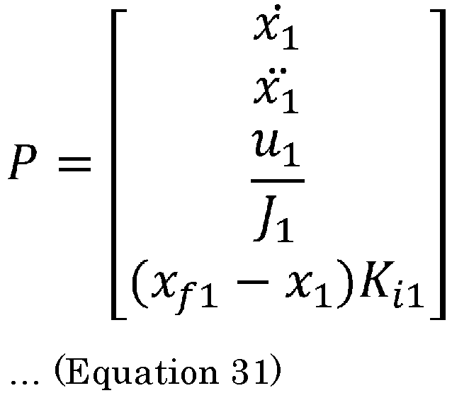
- In the prediction model of Equation 31, a correlation between the expanded state variable and the jerk input u which is a control input is defined. As a result, the model
prediction control unit 43 generates the jerk input u which is a control input on a real-time basis and outputs the jerk input u to the expandedplant 60. In this case, in a calculation process for calculating a stage cost of an evaluation function in model prediction control, the evaluation function (seeEquations 6 to 8) for model prediction control to which the weighting coefficients are set by the parameter setting method illustrated inFig. 4 is used. Since the model prediction control is performed through such parameter setting, an integration amount serving as a driving source of servo control which uses the model prediction control is adjusted ideally, and servo control which suppresses an overshoot can be realized. Furthermore, when a jerk input is used as the control input u, it is possible to easily suppress the largest value of jerk, and therefore, it is possible to ideally suppress vibration of theactual plant 6 during servo control.Fig. 7 illustrates a simulation result when the control structure illustrated inFig. 1A is constructed with respect to the control axes of theactual plant 6 having a plurality of control axes through the parameter setting method and model prediction control is executed on the respective control axes. InFig. 7 , in a working coordinate system in which an output of a first control axis is set as the horizontal axis, an output of a second control axis is set as the vertical axis, the trajectory of a target command is represented by line L3 and the trajectory of the output of theactual plant 6 is represented by line L4. As obvious from the disclosure ofFig. 7 , the output of theactual plant 6 ideally tracks the target command. - Servo control by the
servo driver 4 according to a third configuration example will be described with reference toFig. 8 . In theservo driver 4 of this configuration example, the expandedplant 60 including theactual plant 6 is formed similarly to the second configuration example, afilter unit 7 is incorporated into the expandedplant 60 to form a further expandedplant 600, and model prediction control is performed by the modelprediction control unit 43. In this case, a difference between a target command and the output of the further expanded plant 600 (that is, the output of the actual plant 6) is supplied to aservo integrator 41, and the output z of theservo integrator 41 and the expanded state variable of the further expandedplant 600 are acquired by thestate acquisition unit 42 and are provided to the model prediction control. - Here, the
filter unit 7 performs an attenuation process at a predetermined frequency with respect to the signal (in the present embodiment, the control input u (jerk input) to the further expanded plant 600) input to thefilter unit 7. The predetermined frequency is preferably the frequency of vibration related to theactual plant 6 which is a direct vibration suppression target during servo control. For example, the resonant frequency of theactual plant 6 can be set as the predetermined frequency. Moreover, the attenuation process is a process of attenuating the gain of the signal (control input) related to the predetermined frequency to a desired extent. Therefore, as an example, thefilter unit 7 may be configured as a notch filter in which the predetermined frequency is set as a central frequency of the attenuation process, or may be configured as a low-pass filter in which the predetermined frequency is set as a cutoff frequency of the attenuation process. When thefilter unit 7 is formed in this manner, the signal (the control input u) on which an attenuation process has been performed by thefilter unit 7 is input to the expandedplant 60 including theactual plant 6. As a result, suppression of vibration in theactual plant 6 is expected during servo control of theactual plant 6, and the output of theactual plant 6 can approach a target in a desired period. - Here, on the basis of the fact that the further expanded
plant 600 includes thefilter unit 7 and the expandedplant 60, the prediction model of the modelprediction control unit 43 is determined.Fig. 9 illustrates a transfer function of thefilter unit 7 and a transfer function of the expandedplant 60. An output when the control input u is input to thefilter unit 7 is represented by dv/dt, and the output dv/dt is set as an input to the expandedplant 60. A jerk input is set as the control input u of the present embodiment. -
Fig. 10 illustrates a control structure of the further expandedplant 600 in which the transfer function of thefilter unit 7 and the transfer function of the expandedplant 60 are taken into consideration. Based on the control structure, when the expanded state variable related to the further expandedplant 600 is represented by Equation 32 below, the prediction model of the modelprediction control unit 43 can be represented by Equation 33 below.
[Math. 30]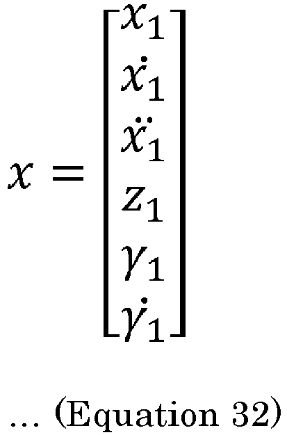
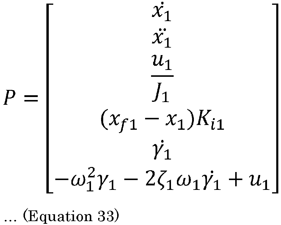
- In the prediction model of Equation 33, a correlation between the expanded state variable and the jerk input u which is a control input is defined. As a result, the model
prediction control unit 43 generates the jerk input u which is a control input on a real-time basis and outputs the jerk input u to thefilter unit 7 included in the further expandedplant 600. Here, when the prediction model (a prediction model represented by Equation 33) of this configuration example is compared with the prediction model (a prediction model represented by Equation 31) of the second configuration example, it is understood that the order of the prediction model of this configuration example is larger than that of the second configuration example by an amount corresponding to the state variable related to thefilter unit 7. Meanwhile, it cannot be said that the state variable related to thefilter unit 7 has a correlation with evaluation (that is, evaluation of optimality based on an evaluation function) of optimality of model prediction control. By taking this into consideration, as for the state quantity cost among the stage costs of the evaluation function for model prediction control of this configuration example, a weighting coefficient corresponding to the state quantity cost is generated using the weighting coefficient obtained in the second configuration example. - Specifically, in the weighting coefficient calculation step (S103) of the parameter setting method illustrated in
Fig. 4 , the weighting coefficients Qf, Q, and R of the evaluation function are calculated according to a prediction model that does not include the state variable of the filter unit 7 (that is, the prediction model of the second configuration example (the prediction model represented by Equation 31)). Since the weighting coefficient Q related to the state quantity cost among these weighting coefficients corresponds to the expandedplant 60 at this time point, the dimension thereof is different from the dimension of the expanded state variable of the further expandedplant 600. Therefore, in order for the dimension of the weighting coefficient Q to correspond to the further expandedplant 600, zeros are added to the weighting coefficient Q by an amount corresponding to the dimension corresponding to the state variable related to thefilter unit 7, and a new weighting coefficient Q' is generated so that the dimension of the weighting coefficient Q corresponds to the dimension of the expanded state variable of the expandedplant 600. - Here,
Fig. 11 illustrates an example of the weighting coefficient Q' related to the state quantity cost. The weighting coefficient Q' inFig. 11 and the weighting coefficient Q which is the base thereof correspond to model prediction control in which the number of control axes is two. The prediction model (a prediction model represented by Equation 33) of this configuration example includes a larger number of state variables than that of the prediction model (the prediction model represented by Equation 31) of the second configuration example by the number (two) of state variables related to thefilter unit 7. Therefore, zeros are added to the weighting coefficient Q by an amount corresponding to the number of dimensions corresponding to this difference to generate a new weighting coefficient Q', which is illustrated inFig. 11 . As described above, since the weighting coefficient Q' illustrated inFig. 11 corresponds to model prediction control in which the number of control axes is two, zeros are added by an amount corresponding to the difference in the number of dimensions corresponding to two control axes. - In the setting step (S104) of the parameter setting method illustrated in
Fig. 4 , the first weighting coefficient Qf (the weighting coefficient Qf calculated according to the prediction model of the second configuration example) is set as the weighting coefficient corresponding to the terminal cost, the new second weighting coefficient Q' is set as the weighting coefficient corresponding to the state quantity cost, and the third weighting coefficient R (the weighting coefficient R calculated according to the prediction model of the second configuration example) is set as the weighting coefficient corresponding to the control input cost. - Since the model prediction control is performed through such parameter setting, an integration amount serving as a driving source of servo control which uses the model prediction control is adjusted ideally, and servo control which suppresses an overshoot can be realized. Furthermore, since the jerk input is set as the control input u and an attenuation process is performed by the
filter unit 7, it is possible to ideally suppress vibration of theactual plant 6 during servo control.Fig. 12 illustrates a simulation result when the control structure illustrated inFig. 1A is constructed with respect to the control axes of theactual plant 6 having a plurality of control axes through the parameter setting method and model prediction control is executed on the respective control axes. InFig. 12 , in a working coordinate system in which an output of a first control axis is set as the horizontal axis, an output of a second control axis is set as the vertical axis, the trajectory of a target command is represented by line L5 and the trajectory of the output of theactual plant 6 is represented by line L6. As obvious from the disclosure ofFig. 12 , the output of theactual plant 6 ideally tracks the target command. - In a fourth configuration example, a control structure which is formed in the
standard PLC 5 and includes a modelprediction control unit 53 corresponding to the modelprediction control unit 43 will be described with reference toFig. 13 . Thestandard PLC 5 includes acommand generation unit 50, anintegrator 51, astate acquisition unit 52, a modelprediction control unit 53, and an expandedplant model 560. Since theintegrator 51, thestate acquisition unit 52, and the modelprediction control unit 53 substantially correspond to theintegrator 41, thestate acquisition unit 42, and the modelprediction control unit 43 illustrated inFigs. 3 ,6 , and8 , respectively, the detailed description thereof will be omitted. - The
command generation unit 50 generates a target command r for instructing the output of theactual plant 6. In this configuration example, the target command r is provided to model prediction control of the modelprediction control unit 53 rather than being supplied from thestandard PLC 5 directly to theservo driver 4. Moreover, the expandedplant model 560 has an expansion system model including a plant model that models the expandedplant 60 illustrated inFigs. 3 and6 or the further expandedplant 600 illustrated inFig. 8 and simulates the output of the expandedplant 60 or the like using the expansion system model. The simulation result is used as an output y of the expandedplant model 560. The output y of the expandedplant model 560 is fed back to an input side of theintegrator 51 by a feedback system. - Here, in this configuration example, an offset e (e = r - y) between the target command r generated by the
command generation unit 50 and the feedback output y of the expandedplant model 560 is input to theintegrator 51. An output z of theintegrator 51 is input to the modelprediction control unit 53 through thestate acquisition unit 52. - Here, the
state acquisition unit 52 acquires the value of a state variable included in the state x related to the expansion system model, provided to the model prediction control performed by the modelprediction control unit 53. The acquisition of the state variable by thestate acquisition unit 52 is substantially the same as acquisition of the state variable by thestate acquisition unit 42 illustrated in the first to third configuration examples described above. The modelprediction control unit 53 executes model prediction control using the state x acquired by thestate acquisition unit 52 and the input u to the expandedplant model 560 output by the modelprediction control unit 53. As for the model prediction control performed by the modelprediction control unit 53, an integral term represented by a product of the offset e and the predetermined integral gain is included in the prediction model used in the model prediction control substantially similarly to the model prediction control performed by the modelprediction control unit 43 illustrated in the first to third configuration examples described above. - Due to the control structure formed in this manner, the
standard PLC 5 illustrated inFig. 13 can supply the output y which is the simulation result of the expandedplant model 560 to theservo driver 4 as a command for ideally tracking the target command r while suppressing the output of theactual plant 6 from entering an overshoot state. That is, thestandard PLC 5 can suppress occurrence of a steady-state offset in the output of theactual plant 6 while performing model prediction control even when the target trajectory changes frequently according to the target command r although the control amount of theactual plant 6 which is the actual control target is not fed back directly. - In the
standard PLC 5 having the control structure configured in this manner, the parameter setting method illustrated inFig. 4 can be applied to the setting of the weighting coefficients of the evaluation function in the model prediction control. When model prediction control is performed in thestandard PLC 5 through such parameter setting, an integration amount serving as a driving source of servo control is adjusted ideally in the servo control for tracking using the model prediction control, it is possible to realize servo control suppressing an overshoot. - A fifth configuration example relates to a modification of the
standard PLC 5 having a control structure including the modelprediction control unit 53 similarly to the fourth configuration example and will be described with reference toFigs. 14 and15 .Fig. 14 illustrates a control structure of thestandard PLC 5 according to this configuration example, and functional units substantially the same as those of thestandard PLC 5 of the fourth configuration example will be denoted by the same reference numerals, and the detailed description thereof will be omitted. In this configuration example, theplant 6 is arobot arm 6 illustrated inFig. 15A . Therefore, the expandedplant model 560 has an expansion system model to which the structure of therobot arm 6 is applied and performs simulation of the expandedplant model 60 using the expansion system model. - Here, the
robot arm 6 which is a plant will be described with reference toFig. 15A . Therobot arm 6 has two motors 2 (motors standard PLC 5. In therobot arm 6, one end of afirst arm 3a is attached to an output shaft of themotor 2a so that thefirst arm 3a is rotated using themotor 2a as a first joint. Furthermore, amotor 2b is disposed at the other end of thefirst arm 3a, and one end of asecond arm 3b is attached to an output shaft of themotor 2b so that thesecond arm 3b is rotated using themotor 2b as a second joint. Atip 3c of thesecond arm 3b is an output unit of therobot arm 6, and an end effector for grasping a predetermined object, for example, is attached to thetip 3c. In therobot arm 6, a plane of rotation of thefirst arm 3a is the same plane as a plane of rotation of thesecond arm 3b, and an x1-axis and an x2-axis are set as orthogonal coordinates for defining the plane of rotation. This orthogonal coordinates are working coordinates related to therobot arm 6, and the position of thetip 3c of therobot arm 6 can be defined on the orthogonal coordinates. Thecommand generation unit 50 of this configuration example generates a predetermined command r that thetip 3c of therobot arm 6 has to track. This command r is based on the working coordinate system (seeFigs. 15A and 15B ) related to therobot arm 6. - Next, a
calculation unit 570 will be described. An output y of the expandedplant model 560 obtained when the control input u is input is based on the working coordinate system illustrated inFigs. 15A and 15B . Meanwhile, themotors robot arm 6 are actuators that are rotated, and a rotation coordinate system which is an independent coordinate system different from the working coordinate system is set to the respective motors for servo control performed by theservo driver 4. Therefore, the output y is not used as a target command for driving themotors calculation unit 570 performs a calculation process for converting the output y of the expandedplant model 560 to a target command based on the rotation coordinate system of the motors. - The calculation process of the
calculation unit 570 is performed according to a geometric relation of an apparatus structure of therobot arm 6.Fig. 15B illustrates the apparatus structure of therobot arm 6. InFig. 15B , the first joint at which themotor 2a is disposed is positioned at the origin of the working coordinate system in order to simplify the description. When the length of thefirst arm 3a is L1, the length of thesecond arm 3b is L2, and the position of thetip 3c is (x1, x2), the rotation angles θ1 and θ2 of themotors robot arm 6 is taken into consideration. The rotation angle θ1 of themotor 2a is defined as the angle between the x1-axis and thefirst arm 3a, and the rotation angle θ2 of themotor 2b is defined as the angle between thefirst arm 3a and thesecond arm 3b.
[Math. 32]
- Here, a function atan2 in Equation 34 is a function that returns a drift angle of (x, y) in the coordinate system when represented by atan2(x, y).
- The angles θ1 and θ2 calculated from the output y of the expanded
plant model 560 by thecalculation unit 570 in this manner are the target commands related to the positions (angles) of the motors, ideal for servo-controlling themotors calculation unit 570 is supplied to theservo driver 4 by asupply unit 580 and is provided to servo control (feedback control) in theservo driver 4. In the control system of the present embodiment, the model prediction control performed in thestandard PLC 5 is performed on the basis of the working coordinate system related to therobot arm 6. Therefore, it is easy to allow the output of therobot arm 6 to ideally track a predetermined command r based on the working coordinate system. Furthermore, through the calculation process of thecalculation unit 570, the result of the model prediction control based on the working coordinate system can be converted to a target command which can be ideally applied to the servo control of themotors robot arm 6, it is possible to ideally avoid occurrence of an output error (position error) of therobot arm 6 resulting from accumulation of computation errors. This is very useful effect in considering the trackability of therobot arm 6. - In the
standard PLC 5 having the control structure configured in this manner, the parameter setting method illustrated inFig. 4 can be applied to the setting of the weighting coefficients of the evaluation function in the model prediction control. Particularly, in this configuration example, since the prediction model of the modelprediction control unit 53 in thestandard PLC 5 is based on the working coordinate system which is an orthogonal coordinate system, it is possible to immediately set the weighting coefficients Qf, Q, and R of the evaluation function according to the parameter setting method and ideally alleviate the load related to the setting. When model prediction control is performed in thestandard PLC 5 through such parameter setting, an integration amount serving as a driving source of servo control is adjusted ideally in the servo control for tracking using the model prediction control, it is possible to realize servo control suppressing an overshoot. - When the
actual plant 6 has a plurality of control axes, the control structure for servo control illustrated in the first to third configuration examples is preferably formed in thestandard PLC 5 as illustrated in the fourth and fifth configuration examples. With such a configuration, it is not necessary to adapt theservo driver 4 to the respective control axes, and it is easy to construct an entire system for servo control of theactual plant 6. The system may naturally be constructed after theservo driver 4 is adapted to the respective control axes. -
- 1
- Network
- 2
- Motor
- 3
- Load device
- 4
- Servo driver
- 5
- Standard PLC
- 6
- Plant
- 6a
- Second integrator
- 7
- Filter unit
- 41
- First integrator
- 42
- State acquisition unit
- 43
- Model prediction control unit
- 50
- Command generation unit
- 51
- Integrator
- 52
- State acquisition unit
- 53
- Model prediction control unit
- 60
- Expanded plant
- 560
- Expanded plant model
- 570
- Calculation unit
- 580
- Supply unit
- 600
- Further expanded plant
Claims (8)
- A method for setting control parameters for model prediction control related to a predetermined control target, the method being executed by a control device having a first integrator to which an offset between a predetermined target command and an output of the predetermined control target corresponding to an actual target device which is an actual target of servo control is input, in order to allow an output of the actual target device tracks the predetermined target command, wherein
the control device includes a model prediction control unit which has a prediction model that defines a correlation between a predetermined expanded state variable related to an expanded control target including at least the predetermined control target and a control input to the expanded control target in a form of a predetermined state equation and which performs the model prediction control based on the prediction model according to a predetermined evaluation function in a prediction section having a predetermined time width with respect to the predetermined target command and outputs a value of the control input at least at an initial time point of the prediction section,
a predetermined state variable which is a portion of the predetermined expanded state variable and is related to the predetermined control target includes a predetermined integral term represented by a product of the offset and a predetermined integral gain, and
the setting method includes:a time response determining step of determining a desired time response in an optimum servo control structure which includes a virtual integrator virtually corresponding to the first integrator and is related to a virtual control target virtually corresponding to the expanded control target and in which, when a virtual target command for the virtual control target is r1, a virtual control input to the virtual control target is a virtual control input u1, and a virtual output of the virtual control target is y1, the virtual control input u1 is represented by Equation 1 below including a state feedback gain KF and an integral gain KI;a gain calculation step of calculating the state feedback gain KF and the integral gain KI corresponding to the desired time response;a weighting coefficient calculation step of calculating a second weighting coefficient Q and a third weighting coefficient R among a first weighting coefficient Qf, the second weighting coefficient Q, and the third weighting coefficient R in a predetermined Riccati equation represented by Equation 3 below on the basis of the state feedback gain KF and the integral gain KI when the control input to the expanded control target is u, the output of the expanded control target is y, the offset is e, the predetermined state variable is x, and a state equation related to the predetermined control target is represented by Equation 2 below; anda setting step of setting the second weighting coefficient Q as a weighting coefficient corresponding to a state quantity cost which is a stage cost related to the predetermined state variable and setting the third weighting coefficient R as a weighting coefficient corresponding to a control input cost which is a stage cost related to the control input in the predetermined evaluation function.
[Math. 1]


- The control parameter setting method for model prediction control according to claim 1, wherein in the weighting coefficient calculation step, the first weighting coefficient Qf is further calculated,
in the setting step, the first weighting coefficient Qf is further set as the weighting coefficient corresponding to the terminal cost related to the predetermined state variable. - The control parameter setting method for model prediction control according to claim 1 or 2, wherein the expanded control target includes the predetermined control target only, and
a portion of the predetermined expanded state variable is identical to the predetermined state variable. - The control parameter setting method for model prediction control according to claim 1, wherein the control input is a jerk input to the predetermined control target,
the expanded control target includes additional integrator that performs a predetermined integration process with respect to the jerk input in addition to the predetermined control target, and
the prediction model defines a correlation between the jerk input and the predetermined expanded state variable including the predetermined state variable related to the predetermined control target and a state variable related to the additional integrator. - The control parameter setting method for model prediction control according to claim 4, wherein a filter unit that performs an attenuation process at a predetermined frequency with respect to a control input based on the predetermined target command is included in the predetermined control target and the expanded control target including the additional integrator whereby a further expanded control target is formed in the control device,
the control parameter setting method for the model prediction control is executed by the control device,
a state variable related to the further expanded control target includes a state variable related to the filter unit in addition to the predetermined expanded state variable,
the prediction model defines a correlation between the jerk input and the predetermined expanded state variable and the state variable related to the filter unit,
in the weighting coefficient calculation step,
the second weighting coefficient Q and the third weighting coefficient R are calculated on the basis of the state feedback gain KF and the integral gain KI, and zeros are added to the second weighting coefficient as a weighting coefficient corresponding to the state variable related to the filter unit so as to correspond to the further expanded control target to obtain a new second weighting coefficient, and
in the setting step,
the new second weighting coefficient is set as the weighting coefficient corresponding to the state quantity cost and the third weighting coefficient R is set as the weighting coefficient corresponding to the control input cost in the predetermined evaluation function. - The control parameter setting method for model prediction control according to claim 2, wherein the control input is a jerk input to the predetermined control target,
the expanded control target includes additional integrator that performs a predetermined integration process with respect to the jerk input in addition to the predetermined control target, and
the prediction model defines a correlation between the jerk input and the predetermined expanded state variable including the predetermined state variable related to the predetermined control target and a state variable related to the additional integrator. - The control parameter setting method for model prediction control according to claim 6, wherein a filter unit that performs an attenuation process at a predetermined frequency with respect to a control input based on the predetermined target command is included in the predetermined control target and the expanded control target including the additional integrator whereby a further expanded control target is formed in the control device,
the control parameter setting method for the model prediction control is executed by the control device,
a state variable related to the further expanded control target includes a state variable related to the filter unit in addition to the predetermined expanded state variable,
the prediction model defines a correlation between the jerk input and the predetermined expanded state variable and the state variable related to the filter unit,
in the weighting coefficient calculation step,
the first weighting coefficient Qf, the second weighting coefficient Q, and the third weighting coefficient R corresponding to the expanded control target are calculated on the basis of the state feedback gain KF and the integral gain KI, and zeros are added to the second weighting coefficient as a weighting coefficient corresponding to a state variable related to the filter unit so as to correspond to the further expanded control target to obtain a new second weighting coefficient, and
in the setting step,
the first weighting coefficient Qf is set as the weighting coefficient corresponding to the terminal cost, the new second weighting coefficient is set as the weighting coefficient corresponding to the state quantity cost, and the third weighting coefficient R is set as the weighting coefficient corresponding to the control input cost in the predetermined evaluation function. - The control parameter setting method for model prediction control according to claim 5 or 7, wherein the filter unit is configured as a notch filter in which the predetermined frequency is used as a central frequency of the attenuation process or a low-pass filter in which the predetermined frequency is used as a cutoff frequency of the attenuation process.
Applications Claiming Priority (2)
| Application Number | Priority Date | Filing Date | Title |
|---|---|---|---|
| JP2018002958 | 2018-01-11 | ||
| PCT/JP2019/000725 WO2019139133A1 (en) | 2018-01-11 | 2019-01-11 | Method for setting control parameters for model prediction control |
Publications (3)
| Publication Number | Publication Date |
|---|---|
| EP3739401A1 true EP3739401A1 (en) | 2020-11-18 |
| EP3739401A4 EP3739401A4 (en) | 2021-10-06 |
| EP3739401B1 EP3739401B1 (en) | 2024-06-26 |
Family
ID=67218644
Family Applications (1)
| Application Number | Title | Priority Date | Filing Date |
|---|---|---|---|
| EP19738282.3A Active EP3739401B1 (en) | 2018-01-11 | 2019-01-11 | Method for setting control parameters for model prediction control |
Country Status (5)
| Country | Link |
|---|---|
| US (1) | US11449032B2 (en) |
| EP (1) | EP3739401B1 (en) |
| JP (1) | JP6958574B2 (en) |
| CN (1) | CN111033396B (en) |
| WO (1) | WO2019139133A1 (en) |
Families Citing this family (8)
| Publication number | Priority date | Publication date | Assignee | Title |
|---|---|---|---|---|
| JP7298085B2 (en) | 2019-07-04 | 2023-06-27 | 三桜工業株式会社 | Manufacturing method and mold for piping joint |
| TWI761975B (en) * | 2020-09-29 | 2022-04-21 | 新加坡商鴻運科股份有限公司 | Device and method for monitoring abnormal machine process parameters, and storage medium |
| CN114851193B (en) * | 2022-04-26 | 2023-12-22 | 北京航空航天大学 | An intelligent and compliant control method for the contact process between a space manipulator and an unknown environment |
| CN116203891B (en) * | 2023-04-28 | 2023-08-04 | 深圳华龙讯达信息技术股份有限公司 | A PLC-based automatic control decision-making optimization method and system |
| CN117311159B (en) * | 2023-10-30 | 2024-10-22 | 上海新华控制技术集团科技有限公司 | Self-adaptive adjusting method and device of control system, storage medium and electronic equipment |
| CN120196075B (en) * | 2025-05-27 | 2025-08-26 | 苏州首拓信息科技有限公司 | Crystal pulling process control method and system of single crystal furnace based on intelligent optimization algorithm |
| CN121657436A (en) * | 2025-11-21 | 2026-03-13 | 北京和利时智能技术有限公司 | A device control method, apparatus, electronic device, and storage medium |
| CN121396043B (en) * | 2025-12-24 | 2026-05-05 | 旋智科技(深圳)有限公司 | Methods, controllers, motor systems, and products for determining filter parameters. |
Family Cites Families (17)
| Publication number | Priority date | Publication date | Assignee | Title |
|---|---|---|---|---|
| JPH01240903A (en) * | 1988-03-23 | 1989-09-26 | Fuji Electric Co Ltd | Method for deciding weight of evaluation function |
| JP3061450B2 (en) * | 1991-07-30 | 2000-07-10 | 株式会社東芝 | Model predictive controller |
| JPH07210210A (en) * | 1994-01-20 | 1995-08-11 | Mitsubishi Heavy Ind Ltd | Hinfinity control designing device |
| JPH09328266A (en) * | 1996-06-12 | 1997-12-22 | Toshiba Corp | Elevator speed controller |
| US6563666B1 (en) * | 1999-04-21 | 2003-05-13 | Seagate Technology Llc | Disc drive model reference seek algorithm |
| US7400933B2 (en) * | 2004-02-06 | 2008-07-15 | Wisconsin Alumni Research Foundation | SISO model predictive controller |
| DE112005001789T5 (en) * | 2004-07-27 | 2007-07-12 | Kabushiki Kaisha Yaskawa Denki, Kitakyushu | Servo control device |
| US7634323B2 (en) * | 2007-02-23 | 2009-12-15 | Toyota Motor Engineering & Manufacturing North America, Inc. | Optimization-based modular control system |
| JP5312688B2 (en) * | 2010-04-26 | 2013-10-09 | 三菱電機株式会社 | Servo control device |
| FR2966617B1 (en) * | 2010-10-22 | 2013-06-14 | Snecma | METHOD AND DEVICE FOR MONITORING A LOOP LOADING A VARIABLE GEOMETRY ACTUATION SYSTEM OF A TURBOJET ENGINE |
| US20120109620A1 (en) * | 2010-11-01 | 2012-05-03 | Honeywell International Inc. | Apparatus and method for model predictive control (mpc) using approximate window-based estimators |
| DE112012006074T5 (en) | 2012-03-21 | 2014-12-04 | Mitsubishi Electric Corporation | Track control apparatus |
| US9378594B2 (en) * | 2014-03-26 | 2016-06-28 | GM Global Technology Operations LLC | Fault diagnostic systems and methods for model predictive control |
| US9235657B1 (en) * | 2013-03-13 | 2016-01-12 | Johnson Controls Technology Company | System identification and model development |
| JP6519457B2 (en) | 2015-11-30 | 2019-05-29 | オムロン株式会社 | Correction device, control method of correction device, information processing program, and recording medium |
| CN107511823B (en) * | 2017-08-29 | 2019-09-27 | 重庆科技学院 | A Method for Optimal Analysis of Robot Trajectory |
| US10759519B2 (en) * | 2017-10-31 | 2020-09-01 | The Boeing Company | Adaptive feedback control of force fighting in hybrid actuation systems |
-
2019
- 2019-01-11 US US16/644,192 patent/US11449032B2/en active Active
- 2019-01-11 JP JP2019003585A patent/JP6958574B2/en not_active Expired - Fee Related
- 2019-01-11 EP EP19738282.3A patent/EP3739401B1/en active Active
- 2019-01-11 CN CN201980003931.8A patent/CN111033396B/en active Active
- 2019-01-11 WO PCT/JP2019/000725 patent/WO2019139133A1/en not_active Ceased
Also Published As
| Publication number | Publication date |
|---|---|
| WO2019139133A1 (en) | 2019-07-18 |
| EP3739401B1 (en) | 2024-06-26 |
| EP3739401A4 (en) | 2021-10-06 |
| US20210064005A1 (en) | 2021-03-04 |
| CN111033396A (en) | 2020-04-17 |
| US11449032B2 (en) | 2022-09-20 |
| JP2019125367A (en) | 2019-07-25 |
| JP6958574B2 (en) | 2021-11-02 |
| CN111033396B (en) | 2023-05-23 |
Similar Documents
| Publication | Publication Date | Title |
|---|---|---|
| EP3739401B1 (en) | Method for setting control parameters for model prediction control | |
| Erkorkmaz et al. | High speed CNC system design. Part I: jerk limited trajectory generation and quintic spline interpolation | |
| CA2744444C (en) | Movement simulator | |
| JP2018173777A (en) | Machine learning device, servo control device, servo control system, and machine learning method | |
| US11106184B2 (en) | Control system | |
| JP6992719B2 (en) | Control device | |
| US20200301376A1 (en) | Machine learning device, control system, and machine learning | |
| JP4269150B2 (en) | Robot controller | |
| US11513497B2 (en) | Control device | |
| CN113260928A (en) | Control device | |
| EP3726301B1 (en) | Control device | |
| Comasolivas et al. | Low level control of an omnidirectional mobile robot | |
| Mujumdar et al. | Control of two link flexible manipulator using higher order sliding modes and disturbance estimation | |
| JP5457894B2 (en) | Full closed position controller | |
| EP3598248B1 (en) | Control system | |
| Leniowska | An adaptive vibration control procedure based on symbolic solution of Diophantine equation | |
| Proaño et al. | Design and Implementation of a Hybrid Sliding Mode Controller with Nonlinear Surface for Trajectory Tracking of a Mobile Manipulator | |
| CN122063867A (en) | Force compensation regulation method based on adaptive control | |
| CN122018289A (en) | Hybrid control method integrating feedforward compensation and self-adaptive fuzzy PID |
Legal Events
| Date | Code | Title | Description |
|---|---|---|---|
| STAA | Information on the status of an ep patent application or granted ep patent |
Free format text: STATUS: THE INTERNATIONAL PUBLICATION HAS BEEN MADE |
|
| PUAI | Public reference made under article 153(3) epc to a published international application that has entered the european phase |
Free format text: ORIGINAL CODE: 0009012 |
|
| STAA | Information on the status of an ep patent application or granted ep patent |
Free format text: STATUS: REQUEST FOR EXAMINATION WAS MADE |
|
| 17P | Request for examination filed |
Effective date: 20200303 |
|
| AK | Designated contracting states |
Kind code of ref document: A1 Designated state(s): AL AT BE BG CH CY CZ DE DK EE ES FI FR GB GR HR HU IE IS IT LI LT LU LV MC MK MT NL NO PL PT RO RS SE SI SK SM TR |
|
| AX | Request for extension of the european patent |
Extension state: BA ME |
|
| DAV | Request for validation of the european patent (deleted) | ||
| DAX | Request for extension of the european patent (deleted) | ||
| A4 | Supplementary search report drawn up and despatched |
Effective date: 20210907 |
|
| RIC1 | Information provided on ipc code assigned before grant |
Ipc: G05B 11/36 20060101ALI20210901BHEP Ipc: G05B 13/04 20060101ALI20210901BHEP Ipc: G05B 17/02 20060101AFI20210901BHEP |
|
| GRAP | Despatch of communication of intention to grant a patent |
Free format text: ORIGINAL CODE: EPIDOSNIGR1 |
|
| STAA | Information on the status of an ep patent application or granted ep patent |
Free format text: STATUS: GRANT OF PATENT IS INTENDED |
|
| INTG | Intention to grant announced |
Effective date: 20240201 |
|
| GRAS | Grant fee paid |
Free format text: ORIGINAL CODE: EPIDOSNIGR3 |
|
| GRAA | (expected) grant |
Free format text: ORIGINAL CODE: 0009210 |
|
| STAA | Information on the status of an ep patent application or granted ep patent |
Free format text: STATUS: THE PATENT HAS BEEN GRANTED |
|
| AK | Designated contracting states |
Kind code of ref document: B1 Designated state(s): AL AT BE BG CH CY CZ DE DK EE ES FI FR GB GR HR HU IE IS IT LI LT LU LV MC MK MT NL NO PL PT RO RS SE SI SK SM TR |
|
| REG | Reference to a national code |
Ref country code: GB Ref legal event code: FG4D |
|
| REG | Reference to a national code |
Ref country code: CH Ref legal event code: EP |
|
| REG | Reference to a national code |
Ref country code: DE Ref legal event code: R096 Ref document number: 602019054209 Country of ref document: DE |
|
| PG25 | Lapsed in a contracting state [announced via postgrant information from national office to epo] |
Ref country code: BG Free format text: LAPSE BECAUSE OF FAILURE TO SUBMIT A TRANSLATION OF THE DESCRIPTION OR TO PAY THE FEE WITHIN THE PRESCRIBED TIME-LIMIT Effective date: 20240626 |
|
| PG25 | Lapsed in a contracting state [announced via postgrant information from national office to epo] |
Ref country code: FI Free format text: LAPSE BECAUSE OF FAILURE TO SUBMIT A TRANSLATION OF THE DESCRIPTION OR TO PAY THE FEE WITHIN THE PRESCRIBED TIME-LIMIT Effective date: 20240626 Ref country code: HR Free format text: LAPSE BECAUSE OF FAILURE TO SUBMIT A TRANSLATION OF THE DESCRIPTION OR TO PAY THE FEE WITHIN THE PRESCRIBED TIME-LIMIT Effective date: 20240626 |
|
| REG | Reference to a national code |
Ref country code: LT Ref legal event code: MG9D |
|
| PG25 | Lapsed in a contracting state [announced via postgrant information from national office to epo] |
Ref country code: GR Free format text: LAPSE BECAUSE OF FAILURE TO SUBMIT A TRANSLATION OF THE DESCRIPTION OR TO PAY THE FEE WITHIN THE PRESCRIBED TIME-LIMIT Effective date: 20240927 |
|
| PG25 | Lapsed in a contracting state [announced via postgrant information from national office to epo] |
Ref country code: LV Free format text: LAPSE BECAUSE OF FAILURE TO SUBMIT A TRANSLATION OF THE DESCRIPTION OR TO PAY THE FEE WITHIN THE PRESCRIBED TIME-LIMIT Effective date: 20240626 |
|
| REG | Reference to a national code |
Ref country code: NL Ref legal event code: MP Effective date: 20240626 |
|
| PG25 | Lapsed in a contracting state [announced via postgrant information from national office to epo] |
Ref country code: NO Free format text: LAPSE BECAUSE OF FAILURE TO SUBMIT A TRANSLATION OF THE DESCRIPTION OR TO PAY THE FEE WITHIN THE PRESCRIBED TIME-LIMIT Effective date: 20240926 Ref country code: LV Free format text: LAPSE BECAUSE OF FAILURE TO SUBMIT A TRANSLATION OF THE DESCRIPTION OR TO PAY THE FEE WITHIN THE PRESCRIBED TIME-LIMIT Effective date: 20240626 Ref country code: HR Free format text: LAPSE BECAUSE OF FAILURE TO SUBMIT A TRANSLATION OF THE DESCRIPTION OR TO PAY THE FEE WITHIN THE PRESCRIBED TIME-LIMIT Effective date: 20240626 Ref country code: GR Free format text: LAPSE BECAUSE OF FAILURE TO SUBMIT A TRANSLATION OF THE DESCRIPTION OR TO PAY THE FEE WITHIN THE PRESCRIBED TIME-LIMIT Effective date: 20240927 Ref country code: FI Free format text: LAPSE BECAUSE OF FAILURE TO SUBMIT A TRANSLATION OF THE DESCRIPTION OR TO PAY THE FEE WITHIN THE PRESCRIBED TIME-LIMIT Effective date: 20240626 Ref country code: BG Free format text: LAPSE BECAUSE OF FAILURE TO SUBMIT A TRANSLATION OF THE DESCRIPTION OR TO PAY THE FEE WITHIN THE PRESCRIBED TIME-LIMIT Effective date: 20240626 Ref country code: RS Free format text: LAPSE BECAUSE OF FAILURE TO SUBMIT A TRANSLATION OF THE DESCRIPTION OR TO PAY THE FEE WITHIN THE PRESCRIBED TIME-LIMIT Effective date: 20240926 |
|
| PG25 | Lapsed in a contracting state [announced via postgrant information from national office to epo] |
Ref country code: NL Free format text: LAPSE BECAUSE OF FAILURE TO SUBMIT A TRANSLATION OF THE DESCRIPTION OR TO PAY THE FEE WITHIN THE PRESCRIBED TIME-LIMIT Effective date: 20240626 |
|
| REG | Reference to a national code |
Ref country code: AT Ref legal event code: MK05 Ref document number: 1698220 Country of ref document: AT Kind code of ref document: T Effective date: 20240626 |
|
| PG25 | Lapsed in a contracting state [announced via postgrant information from national office to epo] |
Ref country code: NL Free format text: LAPSE BECAUSE OF FAILURE TO SUBMIT A TRANSLATION OF THE DESCRIPTION OR TO PAY THE FEE WITHIN THE PRESCRIBED TIME-LIMIT Effective date: 20240626 |
|
| PG25 | Lapsed in a contracting state [announced via postgrant information from national office to epo] |
Ref country code: PT Free format text: LAPSE BECAUSE OF FAILURE TO SUBMIT A TRANSLATION OF THE DESCRIPTION OR TO PAY THE FEE WITHIN THE PRESCRIBED TIME-LIMIT Effective date: 20241028 |
|
| PG25 | Lapsed in a contracting state [announced via postgrant information from national office to epo] |
Ref country code: PT Free format text: LAPSE BECAUSE OF FAILURE TO SUBMIT A TRANSLATION OF THE DESCRIPTION OR TO PAY THE FEE WITHIN THE PRESCRIBED TIME-LIMIT Effective date: 20241028 |
|
| PG25 | Lapsed in a contracting state [announced via postgrant information from national office to epo] |
Ref country code: PL Free format text: LAPSE BECAUSE OF FAILURE TO SUBMIT A TRANSLATION OF THE DESCRIPTION OR TO PAY THE FEE WITHIN THE PRESCRIBED TIME-LIMIT Effective date: 20240626 |
|
| PG25 | Lapsed in a contracting state [announced via postgrant information from national office to epo] |
Ref country code: EE Free format text: LAPSE BECAUSE OF FAILURE TO SUBMIT A TRANSLATION OF THE DESCRIPTION OR TO PAY THE FEE WITHIN THE PRESCRIBED TIME-LIMIT Effective date: 20240626 |
|
| PG25 | Lapsed in a contracting state [announced via postgrant information from national office to epo] |
Ref country code: IS Free format text: LAPSE BECAUSE OF FAILURE TO SUBMIT A TRANSLATION OF THE DESCRIPTION OR TO PAY THE FEE WITHIN THE PRESCRIBED TIME-LIMIT Effective date: 20241026 Ref country code: AT Free format text: LAPSE BECAUSE OF FAILURE TO SUBMIT A TRANSLATION OF THE DESCRIPTION OR TO PAY THE FEE WITHIN THE PRESCRIBED TIME-LIMIT Effective date: 20240626 |
|
| PG25 | Lapsed in a contracting state [announced via postgrant information from national office to epo] |
Ref country code: CZ Free format text: LAPSE BECAUSE OF FAILURE TO SUBMIT A TRANSLATION OF THE DESCRIPTION OR TO PAY THE FEE WITHIN THE PRESCRIBED TIME-LIMIT Effective date: 20240626 |
|
| PG25 | Lapsed in a contracting state [announced via postgrant information from national office to epo] |
Ref country code: RO Free format text: LAPSE BECAUSE OF FAILURE TO SUBMIT A TRANSLATION OF THE DESCRIPTION OR TO PAY THE FEE WITHIN THE PRESCRIBED TIME-LIMIT Effective date: 20240626 Ref country code: SK Free format text: LAPSE BECAUSE OF FAILURE TO SUBMIT A TRANSLATION OF THE DESCRIPTION OR TO PAY THE FEE WITHIN THE PRESCRIBED TIME-LIMIT Effective date: 20240626 |
|
| PG25 | Lapsed in a contracting state [announced via postgrant information from national office to epo] |
Ref country code: ES Free format text: LAPSE BECAUSE OF FAILURE TO SUBMIT A TRANSLATION OF THE DESCRIPTION OR TO PAY THE FEE WITHIN THE PRESCRIBED TIME-LIMIT Effective date: 20240626 Ref country code: SM Free format text: LAPSE BECAUSE OF FAILURE TO SUBMIT A TRANSLATION OF THE DESCRIPTION OR TO PAY THE FEE WITHIN THE PRESCRIBED TIME-LIMIT Effective date: 20240626 |
|
| PG25 | Lapsed in a contracting state [announced via postgrant information from national office to epo] |
Ref country code: SM Free format text: LAPSE BECAUSE OF FAILURE TO SUBMIT A TRANSLATION OF THE DESCRIPTION OR TO PAY THE FEE WITHIN THE PRESCRIBED TIME-LIMIT Effective date: 20240626 Ref country code: SK Free format text: LAPSE BECAUSE OF FAILURE TO SUBMIT A TRANSLATION OF THE DESCRIPTION OR TO PAY THE FEE WITHIN THE PRESCRIBED TIME-LIMIT Effective date: 20240626 Ref country code: RO Free format text: LAPSE BECAUSE OF FAILURE TO SUBMIT A TRANSLATION OF THE DESCRIPTION OR TO PAY THE FEE WITHIN THE PRESCRIBED TIME-LIMIT Effective date: 20240626 Ref country code: PL Free format text: LAPSE BECAUSE OF FAILURE TO SUBMIT A TRANSLATION OF THE DESCRIPTION OR TO PAY THE FEE WITHIN THE PRESCRIBED TIME-LIMIT Effective date: 20240626 Ref country code: IS Free format text: LAPSE BECAUSE OF FAILURE TO SUBMIT A TRANSLATION OF THE DESCRIPTION OR TO PAY THE FEE WITHIN THE PRESCRIBED TIME-LIMIT Effective date: 20241026 Ref country code: ES Free format text: LAPSE BECAUSE OF FAILURE TO SUBMIT A TRANSLATION OF THE DESCRIPTION OR TO PAY THE FEE WITHIN THE PRESCRIBED TIME-LIMIT Effective date: 20240626 Ref country code: EE Free format text: LAPSE BECAUSE OF FAILURE TO SUBMIT A TRANSLATION OF THE DESCRIPTION OR TO PAY THE FEE WITHIN THE PRESCRIBED TIME-LIMIT Effective date: 20240626 Ref country code: CZ Free format text: LAPSE BECAUSE OF FAILURE TO SUBMIT A TRANSLATION OF THE DESCRIPTION OR TO PAY THE FEE WITHIN THE PRESCRIBED TIME-LIMIT Effective date: 20240626 Ref country code: AT Free format text: LAPSE BECAUSE OF FAILURE TO SUBMIT A TRANSLATION OF THE DESCRIPTION OR TO PAY THE FEE WITHIN THE PRESCRIBED TIME-LIMIT Effective date: 20240626 |
|
| PG25 | Lapsed in a contracting state [announced via postgrant information from national office to epo] |
Ref country code: IT Free format text: LAPSE BECAUSE OF FAILURE TO SUBMIT A TRANSLATION OF THE DESCRIPTION OR TO PAY THE FEE WITHIN THE PRESCRIBED TIME-LIMIT Effective date: 20240626 |
|
| REG | Reference to a national code |
Ref country code: DE Ref legal event code: R097 Ref document number: 602019054209 Country of ref document: DE |
|
| PGFP | Annual fee paid to national office [announced via postgrant information from national office to epo] |
Ref country code: DE Payment date: 20250122 Year of fee payment: 7 |
|
| PG25 | Lapsed in a contracting state [announced via postgrant information from national office to epo] |
Ref country code: DK Free format text: LAPSE BECAUSE OF FAILURE TO SUBMIT A TRANSLATION OF THE DESCRIPTION OR TO PAY THE FEE WITHIN THE PRESCRIBED TIME-LIMIT Effective date: 20240626 |
|
| PLBE | No opposition filed within time limit |
Free format text: ORIGINAL CODE: 0009261 |
|
| STAA | Information on the status of an ep patent application or granted ep patent |
Free format text: STATUS: NO OPPOSITION FILED WITHIN TIME LIMIT |
|
| 26N | No opposition filed |
Effective date: 20250327 |
|
| REG | Reference to a national code |
Ref country code: CH Ref legal event code: PL |
|
| PG25 | Lapsed in a contracting state [announced via postgrant information from national office to epo] |
Ref country code: SE Free format text: LAPSE BECAUSE OF FAILURE TO SUBMIT A TRANSLATION OF THE DESCRIPTION OR TO PAY THE FEE WITHIN THE PRESCRIBED TIME-LIMIT Effective date: 20240626 |
|
| PG25 | Lapsed in a contracting state [announced via postgrant information from national office to epo] |
Ref country code: MC Free format text: LAPSE BECAUSE OF FAILURE TO SUBMIT A TRANSLATION OF THE DESCRIPTION OR TO PAY THE FEE WITHIN THE PRESCRIBED TIME-LIMIT Effective date: 20240626 Ref country code: LU Free format text: LAPSE BECAUSE OF NON-PAYMENT OF DUE FEES Effective date: 20250111 |
|
| GBPC | Gb: european patent ceased through non-payment of renewal fee |
Effective date: 20250111 |
|
| PG25 | Lapsed in a contracting state [announced via postgrant information from national office to epo] |
Ref country code: GB Free format text: LAPSE BECAUSE OF NON-PAYMENT OF DUE FEES Effective date: 20250111 Ref country code: BE Free format text: LAPSE BECAUSE OF NON-PAYMENT OF DUE FEES Effective date: 20250131 |
|
| PG25 | Lapsed in a contracting state [announced via postgrant information from national office to epo] |
Ref country code: FR Free format text: LAPSE BECAUSE OF NON-PAYMENT OF DUE FEES Effective date: 20250131 |
|
| PG25 | Lapsed in a contracting state [announced via postgrant information from national office to epo] |
Ref country code: CH Free format text: LAPSE BECAUSE OF NON-PAYMENT OF DUE FEES Effective date: 20250131 |
|
| REG | Reference to a national code |
Ref country code: BE Ref legal event code: MM Effective date: 20250131 |
|
| PG25 | Lapsed in a contracting state [announced via postgrant information from national office to epo] |
Ref country code: IE Free format text: LAPSE BECAUSE OF NON-PAYMENT OF DUE FEES Effective date: 20250111 |
|
| PG25 | Lapsed in a contracting state [announced via postgrant information from national office to epo] |
Ref country code: CY Free format text: LAPSE BECAUSE OF FAILURE TO SUBMIT A TRANSLATION OF THE DESCRIPTION OR TO PAY THE FEE WITHIN THE PRESCRIBED TIME-LIMIT Effective date: 20240626 |
|
| PG25 | Lapsed in a contracting state [announced via postgrant information from national office to epo] |
Ref country code: TR Free format text: LAPSE BECAUSE OF FAILURE TO SUBMIT A TRANSLATION OF THE DESCRIPTION OR TO PAY THE FEE WITHIN THE PRESCRIBED TIME-LIMIT Effective date: 20240626 |
|
| PG25 | Lapsed in a contracting state [announced via postgrant information from national office to epo] |
Ref country code: LT Free format text: LAPSE BECAUSE OF FAILURE TO SUBMIT A TRANSLATION OF THE DESCRIPTION OR TO PAY THE FEE WITHIN THE PRESCRIBED TIME-LIMIT Effective date: 20240626 |