EP3722800B1 - Procédé de détermination de la géométrie d'un point défectueux sur la base d'un procédé de mesure non destructive à l'aide d'une inversion directe - Google Patents
Procédé de détermination de la géométrie d'un point défectueux sur la base d'un procédé de mesure non destructive à l'aide d'une inversion directe Download PDFInfo
- Publication number
- EP3722800B1 EP3722800B1 EP19168531.2A EP19168531A EP3722800B1 EP 3722800 B1 EP3722800 B1 EP 3722800B1 EP 19168531 A EP19168531 A EP 19168531A EP 3722800 B1 EP3722800 B1 EP 3722800B1
- Authority
- EP
- European Patent Office
- Prior art keywords
- expert
- geometry
- defect
- initial
- datasets
- Prior art date
- Legal status (The legal status is an assumption and is not a legal conclusion. Google has not performed a legal analysis and makes no representation as to the accuracy of the status listed.)
- Active
Links
- 230000007547 defect Effects 0.000 title claims description 218
- 238000000034 method Methods 0.000 title claims description 91
- 238000000691 measurement method Methods 0.000 title claims description 46
- 238000013528 artificial neural network Methods 0.000 claims description 82
- 238000005259 measurement Methods 0.000 claims description 63
- 230000001066 destructive effect Effects 0.000 claims description 36
- 238000004088 simulation Methods 0.000 claims description 33
- 238000012549 training Methods 0.000 claims description 31
- 230000007797 corrosion Effects 0.000 claims description 23
- 238000005260 corrosion Methods 0.000 claims description 23
- 238000004422 calculation algorithm Methods 0.000 claims description 20
- 238000003475 lamination Methods 0.000 claims description 19
- BLRBOMBBUUGKFU-SREVYHEPSA-N (z)-4-[[4-(4-chlorophenyl)-5-(2-methoxy-2-oxoethyl)-1,3-thiazol-2-yl]amino]-4-oxobut-2-enoic acid Chemical compound S1C(NC(=O)\C=C/C(O)=O)=NC(C=2C=CC(Cl)=CC=2)=C1CC(=O)OC BLRBOMBBUUGKFU-SREVYHEPSA-N 0.000 claims description 18
- 238000004364 calculation method Methods 0.000 claims description 7
- 230000009467 reduction Effects 0.000 claims description 7
- 238000009826 distribution Methods 0.000 claims description 4
- XLYOFNOQVPJJNP-UHFFFAOYSA-N water Substances O XLYOFNOQVPJJNP-UHFFFAOYSA-N 0.000 claims description 2
- 230000006870 function Effects 0.000 description 19
- 238000013459 approach Methods 0.000 description 10
- 238000011156 evaluation Methods 0.000 description 9
- 230000008859 change Effects 0.000 description 7
- 239000013598 vector Substances 0.000 description 7
- 238000012544 monitoring process Methods 0.000 description 6
- 238000011161 development Methods 0.000 description 5
- 230000005415 magnetization Effects 0.000 description 5
- 239000000463 material Substances 0.000 description 5
- 230000006978 adaptation Effects 0.000 description 4
- 230000000694 effects Effects 0.000 description 4
- 238000005457 optimization Methods 0.000 description 4
- 230000008569 process Effects 0.000 description 4
- 230000008901 benefit Effects 0.000 description 3
- 238000013213 extrapolation Methods 0.000 description 3
- 238000012804 iterative process Methods 0.000 description 3
- 238000010801 machine learning Methods 0.000 description 3
- 239000002184 metal Substances 0.000 description 3
- 238000012545 processing Methods 0.000 description 3
- 238000002604 ultrasonography Methods 0.000 description 3
- 230000002860 competitive effect Effects 0.000 description 2
- 230000004907 flux Effects 0.000 description 2
- 238000007689 inspection Methods 0.000 description 2
- 230000002829 reductive effect Effects 0.000 description 2
- 230000008439 repair process Effects 0.000 description 2
- 238000004513 sizing Methods 0.000 description 2
- 238000005309 stochastic process Methods 0.000 description 2
- 238000012360 testing method Methods 0.000 description 2
- 241001136792 Alle Species 0.000 description 1
- 241000282887 Suidae Species 0.000 description 1
- 230000002411 adverse Effects 0.000 description 1
- 238000009412 basement excavation Methods 0.000 description 1
- 230000005540 biological transmission Effects 0.000 description 1
- 230000002950 deficient Effects 0.000 description 1
- 238000001514 detection method Methods 0.000 description 1
- 238000003384 imaging method Methods 0.000 description 1
- 238000011835 investigation Methods 0.000 description 1
- JEIPFZHSYJVQDO-UHFFFAOYSA-N iron(III) oxide Inorganic materials O=[Fe]O[Fe]=O JEIPFZHSYJVQDO-UHFFFAOYSA-N 0.000 description 1
- 238000010030 laminating Methods 0.000 description 1
- 239000007788 liquid Substances 0.000 description 1
- 230000036961 partial effect Effects 0.000 description 1
- 238000012913 prioritisation Methods 0.000 description 1
- 230000002787 reinforcement Effects 0.000 description 1
- 230000001360 synchronised effect Effects 0.000 description 1
- 230000009466 transformation Effects 0.000 description 1
- 238000000844 transformation Methods 0.000 description 1
- 230000003313 weakening effect Effects 0.000 description 1
Images


Classifications
-
- G—PHYSICS
- G01—MEASURING; TESTING
- G01N—INVESTIGATING OR ANALYSING MATERIALS BY DETERMINING THEIR CHEMICAL OR PHYSICAL PROPERTIES
- G01N27/00—Investigating or analysing materials by the use of electric, electrochemical, or magnetic means
- G01N27/72—Investigating or analysing materials by the use of electric, electrochemical, or magnetic means by investigating magnetic variables
- G01N27/82—Investigating or analysing materials by the use of electric, electrochemical, or magnetic means by investigating magnetic variables for investigating the presence of flaws
- G01N27/90—Investigating or analysing materials by the use of electric, electrochemical, or magnetic means by investigating magnetic variables for investigating the presence of flaws using eddy currents
- G01N27/9046—Investigating or analysing materials by the use of electric, electrochemical, or magnetic means by investigating magnetic variables for investigating the presence of flaws using eddy currents by analysing electrical signals
-
- G—PHYSICS
- G01—MEASURING; TESTING
- G01N—INVESTIGATING OR ANALYSING MATERIALS BY DETERMINING THEIR CHEMICAL OR PHYSICAL PROPERTIES
- G01N29/00—Investigating or analysing materials by the use of ultrasonic, sonic or infrasonic waves; Visualisation of the interior of objects by transmitting ultrasonic or sonic waves through the object
- G01N29/44—Processing the detected response signal, e.g. electronic circuits specially adapted therefor
- G01N29/4481—Neural networks
-
- G—PHYSICS
- G01—MEASURING; TESTING
- G01N—INVESTIGATING OR ANALYSING MATERIALS BY DETERMINING THEIR CHEMICAL OR PHYSICAL PROPERTIES
- G01N27/00—Investigating or analysing materials by the use of electric, electrochemical, or magnetic means
- G01N27/72—Investigating or analysing materials by the use of electric, electrochemical, or magnetic means by investigating magnetic variables
- G01N27/82—Investigating or analysing materials by the use of electric, electrochemical, or magnetic means by investigating magnetic variables for investigating the presence of flaws
-
- G—PHYSICS
- G01—MEASURING; TESTING
- G01N—INVESTIGATING OR ANALYSING MATERIALS BY DETERMINING THEIR CHEMICAL OR PHYSICAL PROPERTIES
- G01N29/00—Investigating or analysing materials by the use of ultrasonic, sonic or infrasonic waves; Visualisation of the interior of objects by transmitting ultrasonic or sonic waves through the object
- G01N29/22—Details, e.g. general constructional or apparatus details
- G01N29/24—Probes
- G01N29/2412—Probes using the magnetostrictive properties of the material to be examined, e.g. electromagnetic acoustic transducers [EMAT]
-
- G—PHYSICS
- G01—MEASURING; TESTING
- G01N—INVESTIGATING OR ANALYSING MATERIALS BY DETERMINING THEIR CHEMICAL OR PHYSICAL PROPERTIES
- G01N29/00—Investigating or analysing materials by the use of ultrasonic, sonic or infrasonic waves; Visualisation of the interior of objects by transmitting ultrasonic or sonic waves through the object
- G01N29/44—Processing the detected response signal, e.g. electronic circuits specially adapted therefor
- G01N29/4409—Processing the detected response signal, e.g. electronic circuits specially adapted therefor by comparison
- G01N29/4427—Processing the detected response signal, e.g. electronic circuits specially adapted therefor by comparison with stored values, e.g. threshold values
-
- G—PHYSICS
- G01—MEASURING; TESTING
- G01N—INVESTIGATING OR ANALYSING MATERIALS BY DETERMINING THEIR CHEMICAL OR PHYSICAL PROPERTIES
- G01N29/00—Investigating or analysing materials by the use of ultrasonic, sonic or infrasonic waves; Visualisation of the interior of objects by transmitting ultrasonic or sonic waves through the object
- G01N29/44—Processing the detected response signal, e.g. electronic circuits specially adapted therefor
- G01N29/4409—Processing the detected response signal, e.g. electronic circuits specially adapted therefor by comparison
- G01N29/4436—Processing the detected response signal, e.g. electronic circuits specially adapted therefor by comparison with a reference signal
-
- G—PHYSICS
- G01—MEASURING; TESTING
- G01N—INVESTIGATING OR ANALYSING MATERIALS BY DETERMINING THEIR CHEMICAL OR PHYSICAL PROPERTIES
- G01N29/00—Investigating or analysing materials by the use of ultrasonic, sonic or infrasonic waves; Visualisation of the interior of objects by transmitting ultrasonic or sonic waves through the object
- G01N29/44—Processing the detected response signal, e.g. electronic circuits specially adapted therefor
- G01N29/4472—Mathematical theories or simulation
Definitions
- the present invention relates to a method for determining the geometry of a defect and a method for determining a load capacity limit of an object that is subjected to pressure at least during operation.
- Such objects are examined for defects using non-destructive measuring methods.
- the results of the measurement methods are evaluated in order to be able to draw conclusions about the type and/or size of defects. Based on this, it can then be determined how much the object can be stressed, for example, or whether and to what extent repair measures or an exchange of the object are necessary. In order to prevent unnecessary measures, it is important to be able to describe the defects and their geometry as precisely as possible.
- An example of an object to be examined in this way is a pipeline.
- One of the main tasks of pipeline inspections, especially with so-called intelligent pigs, is the prediction of safe operating conditions resulting from the condition of the pipeline.
- Pipeline operators are particularly interested in the condition of any welds and the number and size of defects. Defects are, for example, areas with metal losses due to corrosion, cracks or other weakening of a wall of an object provided in particular for storing or transporting liquid or gaseous media. These include, for example, pipes, pipelines or tanks.
- burst pressure Knowledge of the maximum pressure (“burst pressure") applicable to a pipeline above which the pipeline will be destroyed is relevant for the operating pressures that can be set in the pipeline.
- the burst pressure is used to quantitatively determine the resilience limit. Accordingly, accurate prediction of this pressure is important.
- a defect is currently only approximated with regard to its length, width and depth and is therefore regarded as a box.
- this conservative approach is disadvantageous, especially for metal losses due to corrosion on the outside or inside of a pipeline, since the simplified geometric figures necessarily overestimate the current structure of the defect. This leads to the underestimation of the burst pressure of the object and thus to the underestimation of the permitted operating pressures.
- an object that can be operated at higher pressure such as a pipeline or a gas tank, can be operated much more economically.
- MFL examinations are preferably used to find flaws due to corrosion
- other methods in particular using ultrasound, are used to detect cracks on the inside or outside of an object.
- These non-destructive measuring methods include electromagnetic-acoustic methods (EMAT methods), in which sound waves, especially in the form of guided waves, are generated in the pipe wall of the object to be examined due to magnetic fields induced by eddy currents, as well as methods introducing ultrasound directly into the object wall , hereinafter referred to as the ultrasonic method.
- EMAT methods electromagnetic-acoustic methods
- EC measurement methods eddy current measurement methods
- patent document WO-A-2016/007267 discloses a method for determining the geometry of one or more real, examined flaws in a metallic object by means of a reference data set of the object generated on the basis of a non-destructive measuring method.
- patent document US-A-2016/0245779 discloses the use of various non-destructive measurement methods when inspecting an object. The data sets obtained produce prediction data sets by inversion, which are used in an iterative process.
- the object of the present invention is to show a quick way to reconstruct the geometry of a real defect and to calculate the load capacity limit of an object with one or more defects as precisely as possible.
- the geometry of one or more defects is determined by means of at least two reference data records of the object generated using different, non-destructive measurement methods.
- Such a method according to the invention for determining the geometry of one or more real, examined defects of a metallic and in particular magnetizable object, in particular a pipe or a tank, on the basis of at least two reference data sets generated using different, non-destructive measuring methods of the object includes an at least partial representation or imaging of the object on or through an at least two-dimensional, preferably three-dimensional object grid by means of an EDP unit.
- an initial defect geometry is generated in particular on the object grid or an at least two-dimensional defect grid by inverting at least parts of the reference data sets, in particular by at least one neural network trained for these tasks.
- the initial defect geometry can be imaged directly onto the object lattice or represented by it, but it can also be present in a parametric representation, for example on an at least two-dimensional defect lattice.
- the initial defect geometry is determined via a direct inversion. Starting from the result, the reference data sets determined by means of the respective different non-destructive measuring methods, which are based on the results of corresponding measurements, the geometry is deduced, which results in the corresponding measuring results for the different non-destructive measuring methods used.
- the inversion is preferably performed by a neural network trained for this task.
- the neural network can generate output that is assigned to an object grid representing the object. This assigns information about the presence of defects to elements of the object grid, cells or nodes.
- the output can also contain information about the type of defect, such as cracks, corrosion defects or lamination defects, and can be assigned to the object grid.
- the use of at least two reference data sets obtained by different non-destructive measuring methods during the inversion increases the reliability and the accuracy of the method.
- the determination of an initial defect geometry, on the basis of which prediction data sets are calculated for both or all of the reference data sets on which the evaluation is based, which sufficiently match the reference data sets, cannot be obtained by an analytically obtained inverse function, except for the simplest geometries.
- At least one neural network that has been trained for this task is therefore preferably used for the inversion.
- Non-destructive measurement methods are often defect-specific, so that the use of at least two reference data sets obtained by different, non-destructive measurement methods results in surprising synergy effects, especially when using neural networks. While, for example, MFL measurement data often detects corrosion-specific defects and EMAT measurement methods are used more for crack detection, it has been shown that the joint use of corresponding reference data sets not only allows a greater complexity of possible defects to be described and determined, but also that the theoretically available large number of solutions surprisingly solutions with nonsensical geometries are avoided more often. This is attributed to the synergy effects resulting from the training of the neural network in particular by considering the same object and corresponding to the identical defect geometry.
- a training simulation routine preferably generates training data through simulations based on different training geometries, with which a neural network for inverting the measurement data is trained.
- the simulation routine can also be used as the training simulation routine.
- the training geometries each contain different types of defects, each of which is designed differently or has different shapes and dimensions. In particular, this includes both cracks and corrosion defects.
- the training simulation routine can simulate training data for different operating conditions of the non-destructive measuring methods on the basis of the training geometries. For example, different training data for different measurement runs of the non-destructive measurement method, for example with different distances between the sensor and the object, can be simulated for a training geometry.
- Training data can also be generated for the shape of defects contained in different object geometries, for example for an arrangement in a weld seam.
- training data are data pairs from the object geometries or the object grids representing the object geometries with and/or without defects and the reference data records obtained on the basis of the respective geometries.
- the neural network is preferably trained on the basis of data from a database containing simulated measurements.
- a database may contain a variety of different training defect geometries, including, for example, those found in weld shapes.
- a corresponding database preferably contains accumulated data on particularly frequently occurring geometries and/or types of defects.
- a pre-trained neural network can also be trained using database data, but the training is interrupted at an appropriate time.
- the properties of the pre-trained neural network such as the weights of the connections, are saved.
- Another later training of a pre-trained neural network uses the stored properties of the network as a starting point.
- Training data obtained from the simulation of different training geometries are preferably entered into such a database. This reduces the computing effort, since simulations do not have to be carried out several times.
- Input data for the neural network is preferably extracted from a reference data record by a feature extractor, which can also be designed as a further neural network.
- the step of extracting input data from a reference data set is particularly interesting for measurement methods that determine a vector of measurement data for each measurement point, for example in the form of a time series.
- the data most relevant for determining a defect geometry can be selected from the vectors of measurement data of the reference data sets. This selection preferably takes place via a further neural network. This can be done separately or be trained together with the neural network for direct inversion. This procedure reduces the amount of data to be processed in the neural network for the inversion. The procedure can be carried out more easily and quickly.
- the neural network preferably converts input data with a two-dimensional spatial resolution into an output defect geometry with a three-dimensional spatial resolution.
- a neural network with one or more convolutional layers and/or one or more transposed convolutional layers is preferably used for this purpose.
- an input layer of the neural network has a two-dimensional spatial resolution, it being possible for a vector with a plurality of entries to be assigned to an input point of the input layer.
- the neural network is set up to generate an output with a three-dimensional spatial resolution on the basis of this input data, which output can be used as a three-dimensional output defect geometry or can be further converted into a corresponding three-dimensional output defect geometry.
- the three-dimensional initial defect geometry can be used particularly easily for the calculation of a prediction data set by the simulation routine.
- the output of the neural network is assigned to the cells of the object grid.
- individual cells are marked as having or without defects.
- individual defects can then be identified by groups of connected defects Cells are represented, are converted into a parametric defect description on a defect grid, which simplifies any subsequent consideration and processing of the defect geometry.
- a classification of defects preferably takes place.
- defect-specific information is assigned to the detected defects.
- Defects can be differentiated, for example, into surface defects such as corrosion and defects in the volume such as cracks, inclusions or lamination defects.
- lamination defects are regions in which individual materials forming the object are not sufficiently connected to one another, at least locally. This makes it possible to describe the different types of defects, if necessary, in a subsequent iterative adjustment of the initial defect geometry using different defect models. The adjustment of the initial defect geometry in the subsequent iterative method can be more robust, simplified and/or accelerated by the additional information.
- the aforementioned MFL, EMAT, UT and EC measuring methods are different non-destructive measuring methods.
- the method according to the invention is characterized in particular by the fact that a data set based on an MFL, eddy current, EMAT or ultrasound measurement method is used as the first reference data set and a data set generated on the basis of another measurement method originating from this group of measurement methods is used as at least another reference data set becomes. If a measurement method such as an EMAT method generates a data set with a number of sub-data sets, for example on the basis of a number of sensors recording signals, all sub-data sets are then preferably used in the method. In the case of reference data obtained using the EMAT method, the reference data sets are preferably amplitudes ("counts") integrated over time at the respective wall positions or measurement positions, the so-called A-scans.
- the reference data sets generated on the basis of MFL measurements can preferably be additionally differentiated with regard to the direction of the magnetization, ie variants a), b) or c) can thus either contain a reference data set based on an MFL measurement with magnetization in the axial direction (MFL A measurement method) or based on a measurement with magnetization in the circumferential direction (MFL-C measurement method).
- Reference data sets obtained "on the basis" of a specific measurement method come from corresponding measurement runs ("scans") and are optionally prepared for automated processing in the method according to the invention, e.g. they can be normalized with regard to their values and/or interpolated to adapt to specific grid geometries. In particular, they are available as two-dimensional data sets with respective length or width or circumference information and measured values assigned to them.
- the iterative adaptation of the initial defect geometry to the geometry of the real defects is carried out by at least one, preferably a plurality of expert routines that are in particular in competition with each other, each with at least one search strategy or at least one algorithm of their own, which fall back on the same initial defect geometry.
- the expert routines are executed in parallel on an EDP unit. Using a single expert routine, it can access different algorithms for adjusting the defect geometry.
- a respective expert defect geometry is generated by means of at least one proprietary algorithm or a proprietary search strategy and on the basis of the initial defect geometry.
- the expert routine then has its own algorithm if at least one of the algorithms available to the expert routine for adapting the defect geometry differs at least partially from the algorithms of a further expert routine.
- Stochastic processes can preferably be used to differentiate the algorithms of different expert routines.
- Each expert routine has at least one algorithm for adapting the defect geometry, preferably several algorithms are available to at least one expert routine.
- an algorithm can be selected on the basis of stochastic processes or can be specified.
- a measure of the similarity can also be formed via the fitness function, so that, for example, in one embodiment variant, a new initial defect geometry is provided by an expert routine for the further iteration steps even if there is a significant approximation of only one of the simulated or assigned expert prediction data sets to the respective reference data set.
- the calculation of the burst pressure of the examined object can be at least 10% - 20% more accurate and, for example, a pipeline can be operated with higher pressures.
- the examined object has to be inspected less often, for example by excavation.
- the problem of singular, local solutions is minimized via the combined evaluation of data obtained on the basis of different measurement methods, ie the determination of the defect geometry is more robust.
- the expert routines (on the EDP unit) run in competition with one another in such a way that the distribution of the resources of the EDP unit, in particular in the form of computing time, to a respective expert routine depending on a success rate, in which in particular the number of the initial defect geometries calculated by the expert routine and made available for one or more other expert routines is taken into account, and/or depending on a reduction of a fitness function, in which in particular the number of expert prediction data sets generated for the reduction is taken into account .
- the competition between the expert routines results in particular from the fact that the program part designed as a monitoring routine then allocates more resources to the respective expert routines, in particular in the form of computing time, preferably CPU or GPU time, if these are more successful than other expert routines. routines.
- An expert routine is successful when it has found a defect geometry which is provided with a, for example, simulated EMAT measurement that is more suitable for the reference data set and which is made available to the other expert routines.
- a stop criterion is met. This is, for example, a residual difference with regard to the measured and simulated measurement data. It can also be an external stop criterion, for example based on the available computing time or a particularly predeterminable number of iterations or a particularly predeterminable or predetermined computing time or one determined from the available computing time. The stop criterion can also be a combination of these criteria.
- the object grid is also automatically generated from the reference data records.
- a classification of anomaly-free areas and anomaly-prone areas is first carried out on the basis of at least parts of the reference data records Areas of the object, with an initial object grid being created in particular on the basis of previously known information about the object, using the initial object grid, prediction data sets are calculated for the respective non-destructive measurement methods, a comparison of at least parts of the prediction data sets with respective parts of the reference data sets, excluding the anomaly-prone areas, is carried out and depending on at least one measure of accuracy, the initial object grid is used as the object grid describing the geometry of the object, or the EDP unit is used to iteratively adapt the initial object grid to the geometry of the object in the anomaly-free regions.
- Areas of the reference data set that are subject to anomalies are spatial areas that are assigned measurement data that differ significantly from neighboring areas. These anomalies are believed to be due to voids.
- Anomaly-free areas are preferably contiguous areas in which the measured values measured by the non-destructive measuring method do not change or only change within a certain tolerance range, in which the gradient of the change remains below certain limit values, the deviation of individual measured values from an average value is less than a certain threshold value and/or the deviation of a mean value in a local area from adjacent local areas is below a threshold value.
- a starting object grid can be created for determining the object grid, with previously known information about the object, for example the pipeline diameter and the wall thickness in the case of pipelines. Based on the starting object grid, suitable measurements for the respective reference data set are simulated. At least parts of the prediction data record are then compared with at least parts of the at least one reference data record, with the anomaly-prone areas of the reference data record or of the object being excluded in the comparison. If the compared data match with sufficient accuracy, the initial object grid is considered to be a sufficiently accurate representation of the actual shape of the defect-free object and can be used as a basis for evaluating the defects. Otherwise, an iterative adjustment of the initial object grid to the geometry of the object in the anomaly-free areas takes place in the EDP unit.
- a new starting object grid is preferably created and new prediction data records are calculated for this.
- a comparison of at least parts of the new forecast data sets with at least parts of the at least one reference data set, excluding the areas affected by anomalies, is carried out until an object stop criterion for the iterative adjustment, e.g. in the form of an accuracy measure, is reached.
- the initial object grid that is then present is used as the object grid that describes the geometry of the object.
- an interpolation or extrapolation of information from the reference data set and/or object grid from the anomaly-free areas to the anomaly-prone areas takes place.
- the information from the anomaly-free areas can be interpolated and/or extrapolated into the anomaly-prone areas and an auxiliary reference data record obtained in this way can be used to determine the object grid. It is also conceivable to first create an object grid only for the areas classified as free of anomalies.
- This object grid has gaps in the area of the anomaly-affected areas, which can then be closed by interpolation or extrapolation from the anomaly-free areas. In this way, an object grid representing the geometry of the object is obtained, which can then be used for further analyzes of defects or defect geometries in the regions subject to anomalies.
- an anomaly-free area is preferably assigned to at least one predefined local element of the object. This is used when creating the initial object grid or inserted into the initial object grid. This step simplifies creating a seed object mesh.
- the object examined using the non-destructive measuring method can contain weld seams, built-in and/or add-on parts, or have an otherwise previously known, locally modified geometry. The creation of the object grid can be facilitated if this prior information is used.
- attachments such as support elements, clamps, reinforcement elements or, for example, sacrificial anodes of a cathodic rust protection, as well as sleeves attached for repair purposes are predefined in their shape and/or extent.
- the measurement results of the non-destructive measurement methods in these areas naturally look different than in areas of an unchanged wall of the object, for example the pipeline wall in the case of pipelines.
- these changes are uniform and large-scale compared to most defects. Furthermore, they are expected because the elements causing the change are known in their position.
- the classification can be used to identify whether this is a weld seam or a support structure, for example.
- the element recognized in this way can then be used with its known general shape or general dimensions when creating the initial object grid or subsequently introduced into the initial object grid at the appropriate points in order to adapt it to the actual shape of the examined object.
- the respective local element in particular in the form of a weld seam, is particularly preferably described using a parametric geometry model.
- This can significantly reduce the effort involved in creating the object grid.
- the previously known information about the local element is used for this.
- it can be known about a weld seam that extends around the object in the circumferential direction and can be described with sufficient accuracy by a weld seam width and an elevation.
- a predefined parametric geometry model of a local element can be adapted to the actual local shape of the object by varying only a few parameters. This speeds up the process of creating an object grid considerably.
- only one or more parameters of the parametric geometry model can be changed.
- the variation of individual parameters can also be limited by specific limit values within which they can be modified. Such a limitation can minimize the risk of obtaining physically unreasonable results.
- the reliability of the method is increased.
- the object set at the outset is also achieved by a method for determining a load capacity limit of an object that is pressurized at least during operation and is designed in particular as an oil, gas or water pipeline, with the method using a data set describing one or more defects as an input data set in a forward modeling in particular trained calculation of the load limit is used, the input data set is first generated according to the method described above or below for determining the geometry of a defect.
- the advantageous representation of the defect geometry in particular as a non-parametrized real three-dimensional geometry or as a two-dimensional surface with respective depth values, makes simplifications previously assumed to be necessary in the industry superfluous, so that for this reason an increase in the accuracy of the defect determination as a whole in previously cannot be guaranteed.
- the accuracy was limited to specifying the point of the maximum depth of the defect, but now the entire profile is determined with a high level of accuracy.
- the accuracy of the maximum depth is reduced to the extent that can be achieved depending on the measurement accuracy, ie about ⁇ 5% of the wall thickness compared to about ⁇ 10% of the wall thickness with the sizing according to the prior art described at the outset.
- the prediction of the load capacity limit depending on the geometry of the defect achieves increases in accuracy from, for example, ⁇ 50% to ⁇ 5%, especially for critical cases.
- the inventive The advantage lies in particular in an adequate representation of the defect geometry, which is achieved for the first time and which makes this increase possible in the first place.
- a combined data set in this case comprising reference data sets, which were obtained by two different non-destructive measurement methods (EMAT and MFL)
- data are extracted via respective feature extractors (FE) and transferred to a neural network (NN).
- the feature extractors (FE) can be formed by additional neural networks.
- an initial defect geometry is generated via the neural network (NN), which could be the basis for the reference data sets obtained by both or all of the non-destructive measurement methods carried out.
- the neural network (NN) is assigned an input that can consist of one or more vectors that represent a two-dimensional spatial resolution.
- the neural network outputs a vector that represents a three-dimensional spatial resolution.
- This can be assigned to an object grid, whereby individual cells of the object grid are marked as having defects, eg by assigning a value "no material” or "material with defects”. With this marking can additionally preferably be differentiated according to the type of defect such as cracks, corrosion or lamination defects.
- the 2 shows the creation of training data for a corresponding neural network (NN) and the use of this data for training.
- the measurement data 32 obtained by means of a non-destructive measurement method on a corresponding defect geometry are simulated in step 31 or assigned from a database. These are available with a two-dimensional spatial resolution.
- the neural network (NN) has an input layer (ES) whose input points represent a two-dimensional spatial resolution.
- the neural network (NN) is set up to generate an output with a three-dimensional spatial resolution, which is used as a generic defect description 30 or is converted into one.
- Individual data of the measurement data 32 are assigned to the individual grid points of the input layer of the neural network (step 34).
- the position of the defects on the object grid is taken from the generic defect description. In this case, those cells into or through which the defects extend are marked as having defects. This is done by assigning a corresponding value.
- Each cell of the object grid is assigned to the output layer of the neural network with the corresponding information as to whether it has a defect and, if applicable, the type of defect (step 33).
- the neural network is trained in step 37 with these data pairs.
- a training of the neural network can then, for example, by comparing the from the Input layer (ES) assigned data following output with the corresponding data assigned to the output layer of the neural network and an adjustment of weighting factors in the neural network by backpropagation. In this way, the neural network (NN) is trained with a large number of training data sets. If the feature extractors (FE) are also set up as a neural network, they can be trained simultaneously based on the same training data.
- step 3 shows the evaluation of measurement data from a non-destructive measurement method using the neural network (NN).
- Measured values of the non-destructive measuring methods carried out are assigned to the input points of the input layer (ES) of the neural network (NN) (step 34).
- the measured values are measured values from one or more reference data sets.
- the neural network (NN) in step 35 generates an output representing three-dimensional location coordinates. This output is used to create a general defect description, present in the form of an initial defect geometry.
- step 36 the output of the neural network is assigned to the cells of the object grid 30.
- individual cells are identified as having or without defects.
- information about the type of defect in question eg crack, corrosion, lamination defect, can be assigned if necessary.
- individual Defects which are represented by groups of contiguous defective cells, can be converted into a parametric defect description on a defect lattice.
- the surface of a pipe is represented by a 2D mesh surface.
- the defect geometry can be described parameterized as a vector of depth values D lying on a defect lattice.
- This defect geometry is compared with the initial defect geometry on the basis of a result for a fitness function F(x 1 . . . x n ) that takes into account measurement and simulation data belonging to the respective geometry.
- F(x 1 . . . x n ) compared with the initial defect geometry on the basis of a result for a fitness function F(x 1 . . . x n ) that takes into account measurement and simulation data belonging to the respective geometry.
- F(x 1 . . . x n ) a fitness function that takes into account measurement and simulation data belonging to the respective geometry.
- i is the number of data sets to be treated simultaneously (real or simulated data sets)
- Y calories i the result of a simulation of the corresponding i-th measurement
- Y m i are the measured data of the respective reference data sets
- Data sets that are precisely matched to one another can be treated together, with the method according to the invention realizing the simultaneous treatment of the data sets by using a fitness function that takes into account the data sets to be considered together.
- step 7 the reference data sets present in step 6 are accessed, for which purpose in step 8 an initial defect geometry is initially determined as the initial defect geometry. This is done as required on the basis of a neural network into which the reference data sets are read as input data sets.
- the neural network solution is then presented as one or more output defect geometries x 1 .. . x n are made available for the individual expert modules.
- the number of parameter values that describe the defect geometries can be kept as small as possible with the aim of reducing the computing time. This is achieved, for example, via a dynamic grid adjustment. Since the number of depth values corresponds to the number of nodes in the defect lattice 5, the number of nodes can also be the number of defect parameters at the same time. Starting with a comparatively coarse grid, this is successively refined in relevant areas.
- a refinement can be achieved in the relevant grid area, with those cells being successively subdivided that exceed the above depth values.
- the lattice deformation then correlates with the assumed defect geometry, i.e. in areas with large gradients there is a larger number of lattice points.
- a new expert defect geometry is then calculated in step 14 specific to the defect in the respective expert routines and under 14.1 checks whether this must be made available to the other expert routines. This is the case if, for example, a fitness function has been improved as described above and no stop criterion has yet ended the fault finding. In this case, the iteration continues with the defect geometries that are then made available in particular to all expert routines. Otherwise, in 14.2. the process ends with the determination of the defect geometry and, in particular, the statement of the accuracy of the solution. In addition, the burst pressure can be calculated on the basis of the defect geometries found.
- the course of the work flow of a group of expert routines 11, which are in competition with one another, is simulated on the EDP unit.
- the program can have different modules that can set data in specific areas of the EDP unit independently of one another and in particular not synchronized with one another, so that they can be further processed there. This is done in particular under the supervision of a monitoring routine 9 ( figure 5 ).
- a plurality of expert routines 11 thus hold a number of calculation slots 13 depending on the success defined above, ie for example the number of output defect geometries written into a common memory area 12, in order to generate expert defect geometries and/or associated MFL simulations to be able to carry out or to have carried out in the case of an independent MFL simulation module.
- the simulations of the measurement data matching the individual expert defect geometries for the purpose of creating the expert prediction data records are also carried out in the simulation modules 16 under the supervision of the monitoring routine 9 .
- the number of program modules provided for carrying out simulations is preferably equal to the number of slots.
- the monitoring routine 9 monitors the number of iterations and the resulting changes in the initial defect geometry and also monitors whether an associated stop criterion has been reached. Then the result according to block 17, which follows block 14.2 4 corresponds to issued.
- the number of arithmetic slots 13 available for an expert routine 11 and the simulation routines subsequently made available can vary in such a way that a first expert routine, for example, uses up to 50% of the total available for the arithmetic slots and simulation routines computing time can be used.
- the initial defect geometries are stored in the memory area 12, as shown.
- This can be a memory area accessible to the expert routines 11 .
- Log files of expert routines 11 and monitoring routine 9 as well as instructions to the expert routines can also be found there 11 are stored, which are then implemented by them independently. For example, this can be an interrupt command that is set when the stop criterion is reached.
- the expert routines 11 are preferably independent program modules which generate new expert defect geometries and set them in the simulation routines 16 . Furthermore, in the expert routines 11 the fitness function presented at the outset can be generated on the basis of the expert prediction data set and compared with the output prediction data set stored in area 12 . If the expert prediction data records are more similar to the reference data records overall than the data records stored in area 12, these expert prediction data records are then used as new output prediction data records.
- a new defect geometry is generated on a random basis.
- Machine learning algorithms or empirical rules can be used for this.
- the implementation of at least two basic expert routines that work defect-specifically according to the type of defect is provided, as described below.
- These search strategies which are preferably always implemented in a method according to the invention, are based on an assumed probability distribution p(x,y) of grid points for determining a corrosion-based defect geometry, the depth value of which results in a maximum reduction of the fitness function.
- the likelihood function is used to identify N grid points (x n ,y n ). Instead of lattice points x n ,y n , the parameter representation of the group of defects (x 1 ...x n ) already used above can also be assumed as the object of the probability distribution, with N lattice points ( x,y) or (x n ,y n ) is related.
- the depth function which in this case describes the depth D of the corrosion at the lattice point, is changed by ⁇ D, with the sign of the change being distributed randomly.
- D is a set of parameters describing corrosion and is a subset of a common set of parameters describing defect geometry.
- Such an algorithm varies the defect geometry at positions where the simulated MFL measurement signal H the best has the greatest difference to the measured signal H m for the best known solution.
- the monitoring routine 9 shown has, as described, two functions in particular: firstly, whether the stop criterion has been reached is checked and, secondly, the resources of the EDP unit are allocated between the individual experts based on their success.
- the respective non-destructive measurements for the expert defect geometries are simulated in the simulation routines 16 .
- An expert routine can iterate until it finds a solution whose expert prediction data sets are better than the output prediction records stored in area 12. If this is the case, the expert routine 11 can try to achieve further better solutions starting from the already improved solution.
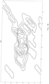
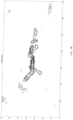
- Figure 6A shows data from a real MFL measurement with magnetization running in the axial direction at a signal strength between 22.2 and 30.6 kA/m
- Figure 6B results from a measurement taken in the circumferential direction (signal strength 22.2 to 91.1 kA/m).
- the contour lines are evenly distributed over the specified area in both figures.
- both EMAT data sets are made available as input data for a neural network by means of a respective input layer.
- the two MFL data sets are also made available to the neural network via the respective input layers.
- the aforementioned burst pressure of 4744.69 kPa results on the basis of the conventional consideration with the determination of the defect geometry established in the state of the art. Based on the method according to the invention results for the MFL data set in the Figure 6F flaw geometry shown (contour lines at 2 mm depth) and based on this a burst pressure of 8543.46 kPa. In the present case, this comes close to 99.4% of the burst pressure, which was determined on the basis of the actual defect geometry determined by laser scanning. Accordingly, a pipeline tested using the method of the present invention can be operated at a safe operating pressure of 6520.53 kPa.
- a model for the non-destructive sensor 21 is created on the basis of measurement data 20 from one or more calibration measurements using a non-destructive measurement method on a calibration object of known geometry, in particular with defects of known geometry.
- a simulation routine is set up in step 22. This can be done by specifying known parameters that represent the material properties and properties of the sensor used. Alternatively or additionally, the parameters can be iteratively adjusted until the results of the simulation routine for the non-destructive measurement method used, based on the known geometry of the calibration object, match the measurement data of the calibration measurement with sufficient accuracy.
- the simulation routine can also be prepared and reused for multiple measurements using the non-destructive measurement method.
- One or more reference data sets are created on the basis of one or more measurements with one or more non-destructive measuring methods.
- 7 shows in step 2 the creation of a reference data set based on several measurement runs.
- a classification into anomaly-free areas and anomaly-prone areas is carried out. Different criteria can be used to distinguish anomaly-free areas from anomaly-prone areas.
- the classification can be further improved by using two or more reference data sets that were obtained on the basis of different non-destructive measurement methods, such that individual measurement methods are more sensitive to certain defects than to others.
- an object grid representing the intact geometry of the object is created in step 24 .
- information from previous measurement runs can also be used in the object, which is then still without defects or has fewer defects.
- the object grid can be created in the anomaly-free areas and then completed by extrapolating and/or interpolating in the anomaly-prone areas. It is also conceivable to carry out an interpolation and/or extrapolation based on the reference data records from the anomaly-free areas into the anomaly-prone areas.
- the object grid is created through an iterative process.
- a first starting object grid is guessed at or specified, for example, on the basis of an estimated object geometry. This is adjusted in an iterative process.
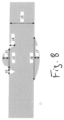
- An initial object grid can, for example, be a weld according to the in 8 have shown in cross section. The initial mesh can be iteratively adjusted until it has a shape representative of the weld.
- a parametric description of the weld seam using a parametric geometry model can also be used.
- 8 shows such a parametric geometry model.
- the shape of the weld is described by a small number of parameters, in this case seven.
- the parameters describe the wall thickness of the object (z5), the respective expansion of the weld seam on both sides (z3, z6), the Weld cant (z1, z7), as well as width and depth of notches on the weld (z2, z4).
- the object grid can thus be changed in the area of the weld seam by adjusting a small number of parameters.
- previously known information about a general shape of an object area here a weld seam, is used.
- the parameters z2, z3, z5, and z6 cannot meaningfully be negative, z4 cannot meaningfully be larger than z5, etc.
- Values for the parameters can be determined using derivation-free optimization algorithms, for example using random search.
- the parameters can be changed in fixed steps, preferably defined as a function of the wall thickness. For example, a change can be made in steps that amount to 1% of the wall thickness.
- the condition of a pipe and thus the pressure that can be specified for safe operation of the pipeline can be specified much more realistically, while operational safety is still guaranteed.
- the inventive method with the resources of the EDP unit competing expert routines, such a result can be made available to the operators of pipelines more quickly or at least in the same evaluation time as in the prior art.
Landscapes
- Physics & Mathematics (AREA)
- Chemical & Material Sciences (AREA)
- General Physics & Mathematics (AREA)
- Health & Medical Sciences (AREA)
- Life Sciences & Earth Sciences (AREA)
- Analytical Chemistry (AREA)
- Biochemistry (AREA)
- General Health & Medical Sciences (AREA)
- Immunology (AREA)
- Pathology (AREA)
- Engineering & Computer Science (AREA)
- Signal Processing (AREA)
- Chemical Kinetics & Catalysis (AREA)
- Electrochemistry (AREA)
- Artificial Intelligence (AREA)
- Evolutionary Computation (AREA)
- Electromagnetism (AREA)
- Mathematical Optimization (AREA)
- Mathematical Analysis (AREA)
- Algebra (AREA)
- Mathematical Physics (AREA)
- Pure & Applied Mathematics (AREA)
- Investigating Or Analyzing Materials By The Use Of Magnetic Means (AREA)
- Testing Resistance To Weather, Investigating Materials By Mechanical Methods (AREA)
- Investigating Or Analyzing Materials By The Use Of Ultrasonic Waves (AREA)
- Monitoring And Testing Of Nuclear Reactors (AREA)
Claims (16)
- Procédé de détermination de la géométrie d'un ou plusieurs points de défaut réels examinés d'un objet métallique, notamment magnétisable, en particulier d'un tube ou d'un réservoir, au moyen d'au moins deux jeux de données de référence de l'objet générés sur la base de procédés de mesure non destructifs différents, l'objet étant représenté au moins partiellement sur ou par une grille d'objet au moins bidimensionnelle, de préférence tridimensionnelle, dans une unité informatique, une géométrie de point de défaut initiale, notamment sur la grille d'objet ou une grille de défaut au moins bidimensionnelle, étant générée par inversion d'au moins des parties des jeux de données de référence, notamment par au moins un réseau neuronal (NN) entraîné pour cette tâche, un jeu de données de prédiction étant respectivement calculé sur la base de la géométrie de point de défaut initiale par une routine de simulation pour les procédés de mesure non destructifs utilisés lors de la création des jeux de données de référence, une comparaison d'au moins des parties des jeux de données de prédiction avec au moins des parties des jeux de données de référence étant effectuée et, en fonction d'au moins une cote de précision, le procédé de détermination de la géométrie du point de défaut prenant fin ou une adaptation itérative de la géométrie de point de défaut initiale à la géométrie du ou des points de défaut réels étant effectuée.
- Procédé selon la revendication 1, caractérisé en ce qu'une routine de simulation d'entraînement génère, par simulation sur la base de différentes géométries d'entraînement, des données d'entraînement avec lesquelles un réseau neuronal (NN) est entraîné pour l'inversion des données de mesure.
- Procédé selon l'une des revendications 1 ou 2, caractérisé en ce qu'un réseau neuronal ou le réseau neuronal (NN) est entraîné sur la base de données issues d'une base de données qui contient des mesures simulées.
- Procédé selon l'une des revendications 1 à 3, caractérisé en ce que des données d'entrée pour le réseau neuronal (NN) sont extraites à partir d'un jeu de données de référence par un extracteur de caractéristique (FE), lequel est de préférence réalisé sous la forme d'un réseau neuronal supplémentaire.
- Procédé selon l'une des revendications 1 à 4, caractérisé en ce que des données d'entrée ayant une résolution spatiale bidimensionnelle sont converties au moyen du réseau neuronal (NN) en une géométrie de point de défaut initiale ayant une résolution spatiale tridimensionnelle.
- Procédé selon l'une des revendications 1 à 5, caractérisé en ce qu'une classification des points de défaut est effectuée par le réseau neuronal (NN).
- Procédé selon l'une des revendications 1 à 6, caractérisé en ce qu'un jeu de données sur la base d'un procédé de mesure MFL, à courant de Foucault, EMAT ou à ultrasons est utilisé en tant que premier jeu de données de référence et un jeu de données généré sur la base d'un procédé de mesure supplémentaire issu de ce groupe de procédés de mesure en tant qu'au moins un jeu de données de référence supplémentaire.
- Procédé selon l'une des revendications 1 à 7, caractérisé en ce que l'adaptation itérative de la géométrie de point de défaut initiale à la géométrie du ou des points de défaut réels est effectuée au moyen de l'unité informatique et au moyen d'au moins une, de préférence plusieurs routines expertes (11) fonctionnant notamment en concurrence et en outre en particulier en parallèle les unes avec les autres,- une géométrie de point de défaut experte étant générée dans la ou les routines expertes (11) respectives au moyen d'au moins un algorithme propre et sur la base de la géométrie de point de défaut initiale,- des jeux de données de prédiction d'expert respectifs étant déterminés sur la base de la géométrie de point de défaut experte respective par simulation ou affectation d'une mesure correspondant au jeu de données de référence respectif,- et la géométrie de point de défaut experte sur laquelle s'appuient les jeux de données de prédiction d'expert respectifs étant ensuite mise à disposition d'au moins une, de préférence de toutes les routines expertes (11) en tant que nouvelle géométrie de point de défaut initiale en vue d'une adaptation supplémentaire à la géométrie du ou des points de défaut réels, lorsque les jeux de données de prédiction d'expert d'une routine experte respective sont plus similaires aux jeux de données de référence respectifs que les jeux de données de prédiction initiaux et/ou une fonction d'adaptation qui tient compte des au moins deux jeux de données de prédiction d'expert est améliorée,- et ensuite les jeux de données de prédiction d'expert qui appartiennent à la nouvelle géométrie de point de défaut initiale étant ensuite utilisés comme nouveaux jeux de données de prédiction initiaux,- l'adaptation itérative au moyen des routines expertes (11) étant effectuée jusqu'à ce qu'un critère d'arrêt soit satisfait.
- Procédé selon la revendication 8, caractérisé en ce que l'adaptation itérative de la géométrie de point de défaut initiale à la géométrie du ou des points de défaut réels est effectuée au moyen d'au moins une routine experte (11) supplémentaire, les routines expertes (11) étant exécutées en concurrence les unes avec les autres de telle sorte qu'une répartition des ressources de l'unité informatique à une routine experte respective s'effectue notamment sous la forme de temps de calcul, de préférence de temps de CPU et/ou de GPU, en fonction d'un taux de réussite, avec lequel est notamment prix en compte le nombre de géométries de point de défaut initiales calculées par cette routine experte et mises à disposition pour une ou plusieurs autres routines expertes (11), et/ou en fonction d'une réduction de la fonction d'adaptation, avec laquelle est notamment pris en compte le nombre de jeux de données de prédiction d'expert générés pour la réduction.
- Procédé selon la revendication 8 ou 9, caractérisé en ce que le critère d'arrêt utilisé et une comparaison de la variation du jeu de données de prédiction d'expert avec la dispersion des mesures du jeu de données réel.
- Procédé selon l'une des revendications 8 à 10, caractérisé en ce que des variations différentes et spécifiques aux points de défaut sont appliquées dans la ou les routines d'expert (11) en vue de générer la géométrie de point de défaut d'expert, une première routine experte (11) étant notamment prévue pour la variation des fissures, une autre pour la variation de la corrosion et/ou une autre pour la variation des défauts de stratification.
- Procédé selon l'une des revendications précédentes, caractérisé en ce que pour la détermination de la grille d'objet, une classification des zones exemptes d'anomalie et des zones qui présentent une anomalie de l'objet est tout d'abord effectuée en se basant au moins sur des parties des jeux de données de référence, une grille d'objet initiale étant créée notamment sur la base d'informations préalablement connues à propos de l'objet, des jeux de données de prédiction étant calculés pour le procédé de mesure non destructif respectif en utilisant la grille d'objet initiale, une comparaison d'au moins des parties des jeux de données de prédiction avec au moins des parties des jeux de données de référence étant effectuée en excluant les zones qui présentent une anomalie et la grille d'objet initiale étant utilisée en fonction d'au moins une cote de précision en tant que grille d'objet qui décrit la géométrie de l'objet ou une adaptation itérative de la grille d'objet initiale à la géométrie de l'objet étant effectuée au moyen de l'unité informatique dans les zones exemptes d'anomalie.
- Procédé selon la revendication 12, caractérisé en ce qu'une nouvelle grille d'objet initiale est créée dans l'adaptation itérative de la grille d'objet initiale et de nouveaux jeux de données de prédiction sont calculés pour celle-ci, et une comparaison d'au moins des parties des nouveaux jeux de données de prédiction avec des parties correspondantes des jeux de données de référence est effectuée en excluant les zones qui présentent une anomalie jusqu'à ce qu'un critère d'arrêt d'objet soit rempli, la grille d'objet initiale alors présente étant utilisée en tant que grille d'objet décrivant la géométrie de l'objet.
- Procédé selon l'une des revendications précédentes 12 ou 13, caractérisé en ce qu'une affectation d'une zone exempte d'anomalie à au moins un élément local prédéfini de l'objet est effectuée lors de la classification et celle-ci est utilisée lors de la création de la grille d'objet initiale ou insérée dans la grille d'objet initiale.
- Procédé selon la revendication 14, caractérisé en ce que l'élément local, qui est notamment réalisé sous la forme d'un cordon de soudure, est décrit au moyen d'un modèle géométrique paramétrique.
- Procédé de détermination d'une limite de capacité de charge d'un objet soumis à une pression au moins pendant le fonctionnement et notamment réalisé sous la forme d'un oléoduc, d'un gazoduc ou d'un pipeline à eau, avec lequel un jeu de données décrivant un ou plusieurs points défauts est utilisé en tant qu'ensemble de données d'entrée dans un calcul de la limite de capacité de charge, caractérisé en ce que le jeu de données d'entrée est tout d'abord déterminé conformément à un procédé selon l'une des revendications précédentes.
Priority Applications (7)
| Application Number | Priority Date | Filing Date | Title |
|---|---|---|---|
| AU2020271967A AU2020271967B2 (en) | 2019-04-09 | 2020-04-09 | Method for determining the geometry of a defect on the basis of non-destructive measurement methods using direct inversion |
| MX2021012416A MX2021012416A (es) | 2019-04-09 | 2020-04-09 | Metodo para determinar la geometria de un defecto a base de metodos de medicion no destructivos mediante el uso de inversion directa. |
| US17/602,957 US20230091681A1 (en) | 2019-04-09 | 2020-04-09 | Method for determining the geometry of a defect based on non-destructive measurement methods using direct inversion |
| CA3136528A CA3136528A1 (fr) | 2019-04-09 | 2020-04-09 | Procede pour determiner la geometrie d'un defaut fonde sur un procede de mesure non destructif au moyen d'une inversion directe |
| BR112021020309A BR112021020309A2 (pt) | 2019-04-09 | 2020-04-09 | Método para determinar a geometria de um defeito com base em métodos de medição não destrutivos usando inversão direta |
| PCT/EP2020/060189 WO2020208155A1 (fr) | 2019-04-09 | 2020-04-09 | Procédé pour déterminer la géométrie d'un défaut fondé sur un procédé de mesure non destructif au moyen d'une inversion directe |
| CONC2021/0015064A CO2021015064A2 (es) | 2019-04-09 | 2021-11-08 | Método para determinar la geometría de un defecto a base de métodos de medición no destructivos mediante el uso de inversión directa |
Applications Claiming Priority (1)
| Application Number | Priority Date | Filing Date | Title |
|---|---|---|---|
| EP19168280 | 2019-04-09 |
Publications (2)
| Publication Number | Publication Date |
|---|---|
| EP3722800A1 EP3722800A1 (fr) | 2020-10-14 |
| EP3722800B1 true EP3722800B1 (fr) | 2023-02-22 |
Family
ID=66334170
Family Applications (1)
| Application Number | Title | Priority Date | Filing Date |
|---|---|---|---|
| EP19168531.2A Active EP3722800B1 (fr) | 2019-04-09 | 2019-04-10 | Procédé de détermination de la géométrie d'un point défectueux sur la base d'un procédé de mesure non destructive à l'aide d'une inversion directe |
Country Status (10)
| Country | Link |
|---|---|
| US (1) | US20230091681A1 (fr) |
| EP (1) | EP3722800B1 (fr) |
| AR (1) | AR118627A1 (fr) |
| AU (1) | AU2020271967B2 (fr) |
| BR (1) | BR112021020309A2 (fr) |
| CA (1) | CA3136528A1 (fr) |
| CO (1) | CO2021015064A2 (fr) |
| ES (1) | ES2942784T3 (fr) |
| MX (1) | MX2021012416A (fr) |
| WO (1) | WO2020208155A1 (fr) |
Families Citing this family (3)
| Publication number | Priority date | Publication date | Assignee | Title |
|---|---|---|---|---|
| EP3722799B1 (fr) * | 2019-04-09 | 2024-09-11 | Rosen IP AG | Procédé de détermination de la géométrie d'un objet en fonction des données du procédé de mesure non destructive |
| US20220404314A1 (en) * | 2021-06-21 | 2022-12-22 | Raytheon Technologies Corporation | System and method for automated indication confirmation in ultrasonic testing |
| CN114199992B (zh) * | 2021-12-02 | 2024-04-05 | 国家石油天然气管网集团有限公司 | 一种储油罐罐壁腐蚀检测方法及系统 |
Family Cites Families (2)
| Publication number | Priority date | Publication date | Assignee | Title |
|---|---|---|---|---|
| EP3126628A4 (fr) * | 2014-07-11 | 2017-11-22 | Halliburton Energy Services, Inc. | Outils d'inspection de tuyau symétriques focalisés |
| WO2016007883A1 (fr) * | 2014-07-11 | 2016-01-14 | Halliburton Energy Services, Inc. | Outil d'évaluation pour tubages de forage concentriques |
-
2019
- 2019-04-10 EP EP19168531.2A patent/EP3722800B1/fr active Active
- 2019-04-10 ES ES19168531T patent/ES2942784T3/es active Active
-
2020
- 2020-04-08 AR ARP200100994A patent/AR118627A1/es active IP Right Grant
- 2020-04-09 AU AU2020271967A patent/AU2020271967B2/en active Active
- 2020-04-09 CA CA3136528A patent/CA3136528A1/fr active Pending
- 2020-04-09 US US17/602,957 patent/US20230091681A1/en active Pending
- 2020-04-09 WO PCT/EP2020/060189 patent/WO2020208155A1/fr active Application Filing
- 2020-04-09 MX MX2021012416A patent/MX2021012416A/es unknown
- 2020-04-09 BR BR112021020309A patent/BR112021020309A2/pt active Search and Examination
-
2021
- 2021-11-08 CO CONC2021/0015064A patent/CO2021015064A2/es unknown
Also Published As
| Publication number | Publication date |
|---|---|
| CA3136528A1 (fr) | 2020-10-15 |
| WO2020208155A1 (fr) | 2020-10-15 |
| BR112021020309A2 (pt) | 2021-12-14 |
| US20230091681A1 (en) | 2023-03-23 |
| AR118627A1 (es) | 2021-10-20 |
| AU2020271967A1 (en) | 2021-11-04 |
| EP3722800A1 (fr) | 2020-10-14 |
| ES2942784T3 (es) | 2023-06-06 |
| MX2021012416A (es) | 2022-02-10 |
| CO2021015064A2 (es) | 2021-11-19 |
| AU2020271967B2 (en) | 2023-11-16 |
Similar Documents
| Publication | Publication Date | Title |
|---|---|---|
| EP3722800B1 (fr) | Procédé de détermination de la géométrie d'un point défectueux sur la base d'un procédé de mesure non destructive à l'aide d'une inversion directe | |
| EP3044571B1 (fr) | Procédé et dispositif de vérification d'un système d'inspection servant à détecter des défauts de surfaces | |
| EP3268713B1 (fr) | Procédé de réalisation d'un ensemble de modèles permettant d'étalonner un appareil de commande | |
| DE602004007753T2 (de) | Verfahren zur Qualitätskontrolle eines industriellen Verfahrens, insbesondere eines Laserschweissverfahrens | |
| EP3213294A1 (fr) | Détermination d'un indice de qualité à partir d'un jeu de données d'une image volumique | |
| DE102013211616A1 (de) | Verfahren und Vorrichtung zur Defektgrößenbewertung | |
| EP3722798B1 (fr) | Procédé de détermination de la géométrie d'un point défectueux et de détermination de la capacité de charge | |
| WO2020212489A1 (fr) | Procédé mis en œuvre par ordinateur pour la détermination de défauts d'un objet fabriqué au moyen d'un processus de fabrication additif | |
| DE112018003588T5 (de) | Restlebensdauer-Bewertungsverfahren und Instandhaltungsverwaltungsverfahren | |
| EP3692362A1 (fr) | Procédé de détermination de la géométrie d'un défaut et de détermination de la limite de charge | |
| DE112018003282T5 (de) | Riss-Evaluierungskriteriums-Formulierungsverfahren, Riss-Evaluierungsverfahren durch interne Fehlerinspektion und Wartungsverwaltungsverfahren | |
| EP3722799B1 (fr) | Procédé de détermination de la géométrie d'un objet en fonction des données du procédé de mesure non destructive | |
| DE102016200779A1 (de) | Untersuchungsverfahren für ein zu wartendes hohles Bauteil einer Strömungsmaschine | |
| EP2821783B1 (fr) | Dispositif et procédé de détermination de défauts matériels dans des éprouvettes à symétrie de révolution au moyen d'ultrasons | |
| EP1421559B1 (fr) | Dispositif et procede permettant d'evaluer la qualite d'un objet | |
| EP0296461B1 (fr) | Procédé pour l'essai de composants | |
| DE112020006580T5 (de) | Riss-schätzeinrichtung, riss-schätzverfahren, riss-überprüfungsverfahren und defekt-diagnoseverfahren | |
| EP3814742A1 (fr) | Procédé de contrôle d'au moins une partie d'une pièce et dispositif de contrôle servant au contrôle d'au moins une partie d'une pièce | |
| DE102023201749A1 (de) | Verfahren zum Trainieren eines Ensemble Algorithmus des maschinellen Lernens zum Klassifizieren von Bilddaten | |
| DE102016224364A1 (de) | Verfahren und Vorrichtung zur zerstörungsfreien Prüfung eines Objektes | |
| DE20114104U1 (de) | Vorrichtung zum Auswerten einer Beschaffenheit eines Objekts |
Legal Events
| Date | Code | Title | Description |
|---|---|---|---|
| PUAI | Public reference made under article 153(3) epc to a published international application that has entered the european phase |
Free format text: ORIGINAL CODE: 0009012 |
|
| STAA | Information on the status of an ep patent application or granted ep patent |
Free format text: STATUS: THE APPLICATION HAS BEEN PUBLISHED |
|
| AK | Designated contracting states |
Kind code of ref document: A1 Designated state(s): AL AT BE BG CH CY CZ DE DK EE ES FI FR GB GR HR HU IE IS IT LI LT LU LV MC MK MT NL NO PL PT RO RS SE SI SK SM TR |
|
| AX | Request for extension of the european patent |
Extension state: BA ME |
|
| STAA | Information on the status of an ep patent application or granted ep patent |
Free format text: STATUS: REQUEST FOR EXAMINATION WAS MADE |
|
| 17P | Request for examination filed |
Effective date: 20210412 |
|
| RBV | Designated contracting states (corrected) |
Designated state(s): AL AT BE BG CH CY CZ DE DK EE ES FI FR GB GR HR HU IE IS IT LI LT LU LV MC MK MT NL NO PL PT RO RS SE SI SK SM TR |
|
| GRAP | Despatch of communication of intention to grant a patent |
Free format text: ORIGINAL CODE: EPIDOSNIGR1 |
|
| STAA | Information on the status of an ep patent application or granted ep patent |
Free format text: STATUS: GRANT OF PATENT IS INTENDED |
|
| INTG | Intention to grant announced |
Effective date: 20220908 |
|
| GRAS | Grant fee paid |
Free format text: ORIGINAL CODE: EPIDOSNIGR3 |
|
| GRAA | (expected) grant |
Free format text: ORIGINAL CODE: 0009210 |
|
| STAA | Information on the status of an ep patent application or granted ep patent |
Free format text: STATUS: THE PATENT HAS BEEN GRANTED |
|
| AK | Designated contracting states |
Kind code of ref document: B1 Designated state(s): AL AT BE BG CH CY CZ DE DK EE ES FI FR GB GR HR HU IE IS IT LI LT LU LV MC MK MT NL NO PL PT RO RS SE SI SK SM TR |
|
| REG | Reference to a national code |
Ref country code: GB Ref legal event code: FG4D Free format text: NOT ENGLISH |
|
| REG | Reference to a national code |
Ref country code: CH Ref legal event code: EP |
|
| REG | Reference to a national code |
Ref country code: DE Ref legal event code: R096 Ref document number: 502019007008 Country of ref document: DE |
|
| REG | Reference to a national code |
Ref country code: AT Ref legal event code: REF Ref document number: 1549834 Country of ref document: AT Kind code of ref document: T Effective date: 20230315 Ref country code: IE Ref legal event code: FG4D Free format text: LANGUAGE OF EP DOCUMENT: GERMAN |
|
| REG | Reference to a national code |
Ref country code: NL Ref legal event code: FP |
|
| REG | Reference to a national code |
Ref country code: NO Ref legal event code: T2 Effective date: 20230222 |
|
| REG | Reference to a national code |
Ref country code: ES Ref legal event code: FG2A Ref document number: 2942784 Country of ref document: ES Kind code of ref document: T3 Effective date: 20230606 |
|
| REG | Reference to a national code |
Ref country code: LT Ref legal event code: MG9D |
|
| PG25 | Lapsed in a contracting state [announced via postgrant information from national office to epo] |
Ref country code: RS Free format text: LAPSE BECAUSE OF FAILURE TO SUBMIT A TRANSLATION OF THE DESCRIPTION OR TO PAY THE FEE WITHIN THE PRESCRIBED TIME-LIMIT Effective date: 20230222 Ref country code: PT Free format text: LAPSE BECAUSE OF FAILURE TO SUBMIT A TRANSLATION OF THE DESCRIPTION OR TO PAY THE FEE WITHIN THE PRESCRIBED TIME-LIMIT Effective date: 20230622 Ref country code: LV Free format text: LAPSE BECAUSE OF FAILURE TO SUBMIT A TRANSLATION OF THE DESCRIPTION OR TO PAY THE FEE WITHIN THE PRESCRIBED TIME-LIMIT Effective date: 20230222 Ref country code: LT Free format text: LAPSE BECAUSE OF FAILURE TO SUBMIT A TRANSLATION OF THE DESCRIPTION OR TO PAY THE FEE WITHIN THE PRESCRIBED TIME-LIMIT Effective date: 20230222 Ref country code: HR Free format text: LAPSE BECAUSE OF FAILURE TO SUBMIT A TRANSLATION OF THE DESCRIPTION OR TO PAY THE FEE WITHIN THE PRESCRIBED TIME-LIMIT Effective date: 20230222 |
|
| PG25 | Lapsed in a contracting state [announced via postgrant information from national office to epo] |
Ref country code: SE Free format text: LAPSE BECAUSE OF FAILURE TO SUBMIT A TRANSLATION OF THE DESCRIPTION OR TO PAY THE FEE WITHIN THE PRESCRIBED TIME-LIMIT Effective date: 20230222 Ref country code: PL Free format text: LAPSE BECAUSE OF FAILURE TO SUBMIT A TRANSLATION OF THE DESCRIPTION OR TO PAY THE FEE WITHIN THE PRESCRIBED TIME-LIMIT Effective date: 20230222 Ref country code: IS Free format text: LAPSE BECAUSE OF FAILURE TO SUBMIT A TRANSLATION OF THE DESCRIPTION OR TO PAY THE FEE WITHIN THE PRESCRIBED TIME-LIMIT Effective date: 20230622 Ref country code: GR Free format text: LAPSE BECAUSE OF FAILURE TO SUBMIT A TRANSLATION OF THE DESCRIPTION OR TO PAY THE FEE WITHIN THE PRESCRIBED TIME-LIMIT Effective date: 20230523 Ref country code: FI Free format text: LAPSE BECAUSE OF FAILURE TO SUBMIT A TRANSLATION OF THE DESCRIPTION OR TO PAY THE FEE WITHIN THE PRESCRIBED TIME-LIMIT Effective date: 20230222 |
|
| REG | Reference to a national code |
Ref country code: DE Ref legal event code: R081 Ref document number: 502019007008 Country of ref document: DE Owner name: ROSEN IP AG, CH Free format text: FORMER OWNER: ROSEN SWISS AG, STANS, CH |
|
| PG25 | Lapsed in a contracting state [announced via postgrant information from national office to epo] |
Ref country code: SM Free format text: LAPSE BECAUSE OF FAILURE TO SUBMIT A TRANSLATION OF THE DESCRIPTION OR TO PAY THE FEE WITHIN THE PRESCRIBED TIME-LIMIT Effective date: 20230222 Ref country code: RO Free format text: LAPSE BECAUSE OF FAILURE TO SUBMIT A TRANSLATION OF THE DESCRIPTION OR TO PAY THE FEE WITHIN THE PRESCRIBED TIME-LIMIT Effective date: 20230222 Ref country code: EE Free format text: LAPSE BECAUSE OF FAILURE TO SUBMIT A TRANSLATION OF THE DESCRIPTION OR TO PAY THE FEE WITHIN THE PRESCRIBED TIME-LIMIT Effective date: 20230222 Ref country code: DK Free format text: LAPSE BECAUSE OF FAILURE TO SUBMIT A TRANSLATION OF THE DESCRIPTION OR TO PAY THE FEE WITHIN THE PRESCRIBED TIME-LIMIT Effective date: 20230222 Ref country code: CZ Free format text: LAPSE BECAUSE OF FAILURE TO SUBMIT A TRANSLATION OF THE DESCRIPTION OR TO PAY THE FEE WITHIN THE PRESCRIBED TIME-LIMIT Effective date: 20230222 |
|
| REG | Reference to a national code |
Ref country code: DE Ref legal event code: R097 Ref document number: 502019007008 Country of ref document: DE |
|
| PG25 | Lapsed in a contracting state [announced via postgrant information from national office to epo] |
Ref country code: SK Free format text: LAPSE BECAUSE OF FAILURE TO SUBMIT A TRANSLATION OF THE DESCRIPTION OR TO PAY THE FEE WITHIN THE PRESCRIBED TIME-LIMIT Effective date: 20230222 |
|
| REG | Reference to a national code |
Ref country code: CH Ref legal event code: PL |
|
| RAP2 | Party data changed (patent owner data changed or rights of a patent transferred) |
Owner name: ROSEN IP AG |
|
| PG25 | Lapsed in a contracting state [announced via postgrant information from national office to epo] |
Ref country code: LU Free format text: LAPSE BECAUSE OF NON-PAYMENT OF DUE FEES Effective date: 20230410 |
|
| PLBE | No opposition filed within time limit |
Free format text: ORIGINAL CODE: 0009261 |
|
| STAA | Information on the status of an ep patent application or granted ep patent |
Free format text: STATUS: NO OPPOSITION FILED WITHIN TIME LIMIT |
|
| REG | Reference to a national code |
Ref country code: GB Ref legal event code: 732E Free format text: REGISTERED BETWEEN 20231207 AND 20231213 |
|
| REG | Reference to a national code |
Ref country code: BE Ref legal event code: MM Effective date: 20230430 |
|
| PG25 | Lapsed in a contracting state [announced via postgrant information from national office to epo] |
Ref country code: MC Free format text: LAPSE BECAUSE OF FAILURE TO SUBMIT A TRANSLATION OF THE DESCRIPTION OR TO PAY THE FEE WITHIN THE PRESCRIBED TIME-LIMIT Effective date: 20230222 |
|
| 26N | No opposition filed |
Effective date: 20231123 |
|
| PG25 | Lapsed in a contracting state [announced via postgrant information from national office to epo] |
Ref country code: SI Free format text: LAPSE BECAUSE OF FAILURE TO SUBMIT A TRANSLATION OF THE DESCRIPTION OR TO PAY THE FEE WITHIN THE PRESCRIBED TIME-LIMIT Effective date: 20230222 Ref country code: MC Free format text: LAPSE BECAUSE OF FAILURE TO SUBMIT A TRANSLATION OF THE DESCRIPTION OR TO PAY THE FEE WITHIN THE PRESCRIBED TIME-LIMIT Effective date: 20230222 Ref country code: LI Free format text: LAPSE BECAUSE OF NON-PAYMENT OF DUE FEES Effective date: 20230430 Ref country code: CH Free format text: LAPSE BECAUSE OF NON-PAYMENT OF DUE FEES Effective date: 20230430 |
|
| REG | Reference to a national code |
Ref country code: IE Ref legal event code: MM4A |
|
| PG25 | Lapsed in a contracting state [announced via postgrant information from national office to epo] |
Ref country code: BE Free format text: LAPSE BECAUSE OF NON-PAYMENT OF DUE FEES Effective date: 20230430 |
|
| PG25 | Lapsed in a contracting state [announced via postgrant information from national office to epo] |
Ref country code: IE Free format text: LAPSE BECAUSE OF NON-PAYMENT OF DUE FEES Effective date: 20230410 |
|
| PG25 | Lapsed in a contracting state [announced via postgrant information from national office to epo] |
Ref country code: IE Free format text: LAPSE BECAUSE OF NON-PAYMENT OF DUE FEES Effective date: 20230410 |
|
| PGFP | Annual fee paid to national office [announced via postgrant information from national office to epo] |
Ref country code: NL Payment date: 20240422 Year of fee payment: 6 |
|
| PGFP | Annual fee paid to national office [announced via postgrant information from national office to epo] |
Ref country code: GB Payment date: 20240423 Year of fee payment: 6 |
|
| PGFP | Annual fee paid to national office [announced via postgrant information from national office to epo] |
Ref country code: DE Payment date: 20240418 Year of fee payment: 6 |
|
| PGFP | Annual fee paid to national office [announced via postgrant information from national office to epo] |
Ref country code: ES Payment date: 20240517 Year of fee payment: 6 |
|
| PGFP | Annual fee paid to national office [announced via postgrant information from national office to epo] |
Ref country code: NO Payment date: 20240419 Year of fee payment: 6 Ref country code: IT Payment date: 20240430 Year of fee payment: 6 Ref country code: FR Payment date: 20240419 Year of fee payment: 6 |
|
| REG | Reference to a national code |
Ref country code: NL Ref legal event code: PD Owner name: ROSEN IP AG; CH Free format text: DETAILS ASSIGNMENT: CHANGE OF OWNER(S), ASSIGNMENT; FORMER OWNER NAME: ROSEN SWISS AG Effective date: 20240808 |