EP3577491B1 - System and method for speed and attenuation reconstruction in ultrasound imaging - Google Patents
System and method for speed and attenuation reconstruction in ultrasound imaging Download PDFInfo
- Publication number
- EP3577491B1 EP3577491B1 EP18709958.5A EP18709958A EP3577491B1 EP 3577491 B1 EP3577491 B1 EP 3577491B1 EP 18709958 A EP18709958 A EP 18709958A EP 3577491 B1 EP3577491 B1 EP 3577491B1
- Authority
- EP
- European Patent Office
- Prior art keywords
- ultrasound
- transducer
- processor
- medical
- tissue
- Prior art date
- Legal status (The legal status is an assumption and is not a legal conclusion. Google has not performed a legal analysis and makes no representation as to the accuracy of the status listed.)
- Active
Links
- 238000000034 method Methods 0.000 title claims description 62
- 238000012285 ultrasound imaging Methods 0.000 title description 3
- 238000002604 ultrasonography Methods 0.000 claims description 277
- 238000005259 measurement Methods 0.000 claims description 107
- 239000011159 matrix material Substances 0.000 claims description 33
- 230000001419 dependent effect Effects 0.000 claims description 21
- 238000005457 optimization Methods 0.000 claims description 7
- 230000005855 radiation Effects 0.000 claims description 6
- 230000004044 response Effects 0.000 claims description 5
- 238000004364 calculation method Methods 0.000 claims description 4
- 230000001186 cumulative effect Effects 0.000 claims description 4
- 238000012545 processing Methods 0.000 claims description 4
- 210000001519 tissue Anatomy 0.000 description 108
- 238000006073 displacement reaction Methods 0.000 description 33
- 230000006870 function Effects 0.000 description 28
- 238000009826 distribution Methods 0.000 description 17
- 210000000481 breast Anatomy 0.000 description 13
- 238000004422 calculation algorithm Methods 0.000 description 13
- 230000003902 lesion Effects 0.000 description 13
- 238000013459 approach Methods 0.000 description 11
- 206010028980 Neoplasm Diseases 0.000 description 10
- 238000002591 computed tomography Methods 0.000 description 10
- 230000008569 process Effects 0.000 description 10
- 238000003384 imaging method Methods 0.000 description 9
- 238000010304 firing Methods 0.000 description 8
- 239000000523 sample Substances 0.000 description 8
- 230000001934 delay Effects 0.000 description 7
- 238000002310 reflectometry Methods 0.000 description 7
- 230000005540 biological transmission Effects 0.000 description 6
- 230000004069 differentiation Effects 0.000 description 6
- 230000033001 locomotion Effects 0.000 description 6
- 230000008901 benefit Effects 0.000 description 5
- 238000002592 echocardiography Methods 0.000 description 4
- 210000000056 organ Anatomy 0.000 description 4
- 238000004088 simulation Methods 0.000 description 4
- 238000003325 tomography Methods 0.000 description 4
- 238000004458 analytical method Methods 0.000 description 3
- 201000011510 cancer Diseases 0.000 description 3
- 238000003745 diagnosis Methods 0.000 description 3
- 238000010586 diagram Methods 0.000 description 3
- 239000006185 dispersion Substances 0.000 description 3
- 230000005284 excitation Effects 0.000 description 3
- 210000004185 liver Anatomy 0.000 description 3
- 230000007246 mechanism Effects 0.000 description 3
- 230000010363 phase shift Effects 0.000 description 3
- 238000005070 sampling Methods 0.000 description 3
- 210000004872 soft tissue Anatomy 0.000 description 3
- 238000013334 tissue model Methods 0.000 description 3
- 206010001233 Adenoma benign Diseases 0.000 description 2
- 208000007659 Fibroadenoma Diseases 0.000 description 2
- 238000011298 ablation treatment Methods 0.000 description 2
- 239000000090 biomarker Substances 0.000 description 2
- 238000001574 biopsy Methods 0.000 description 2
- 210000000988 bone and bone Anatomy 0.000 description 2
- 201000003149 breast fibroadenoma Diseases 0.000 description 2
- 239000003086 colorant Substances 0.000 description 2
- 238000000354 decomposition reaction Methods 0.000 description 2
- 238000001514 detection method Methods 0.000 description 2
- 230000000694 effects Effects 0.000 description 2
- 238000002091 elastography Methods 0.000 description 2
- 210000003734 kidney Anatomy 0.000 description 2
- 230000000704 physical effect Effects 0.000 description 2
- 230000009467 reduction Effects 0.000 description 2
- 230000003595 spectral effect Effects 0.000 description 2
- 238000012360 testing method Methods 0.000 description 2
- 230000001960 triggered effect Effects 0.000 description 2
- XLYOFNOQVPJJNP-UHFFFAOYSA-N water Substances O XLYOFNOQVPJJNP-UHFFFAOYSA-N 0.000 description 2
- 108050005509 3D domains Proteins 0.000 description 1
- 206010006187 Breast cancer Diseases 0.000 description 1
- 208000026310 Breast neoplasm Diseases 0.000 description 1
- 101100129500 Caenorhabditis elegans max-2 gene Proteins 0.000 description 1
- 238000010521 absorption reaction Methods 0.000 description 1
- 238000009825 accumulation Methods 0.000 description 1
- 238000007792 addition Methods 0.000 description 1
- 239000000654 additive Substances 0.000 description 1
- 230000000996 additive effect Effects 0.000 description 1
- 230000004075 alteration Effects 0.000 description 1
- 238000003491 array Methods 0.000 description 1
- 230000004888 barrier function Effects 0.000 description 1
- 230000002146 bilateral effect Effects 0.000 description 1
- 210000004204 blood vessel Anatomy 0.000 description 1
- 210000004556 brain Anatomy 0.000 description 1
- 230000015556 catabolic process Effects 0.000 description 1
- 230000008859 change Effects 0.000 description 1
- 238000006243 chemical reaction Methods 0.000 description 1
- 230000001427 coherent effect Effects 0.000 description 1
- 230000000052 comparative effect Effects 0.000 description 1
- 230000000295 complement effect Effects 0.000 description 1
- 230000006835 compression Effects 0.000 description 1
- 238000007906 compression Methods 0.000 description 1
- 230000003750 conditioning effect Effects 0.000 description 1
- 230000001955 cumulated effect Effects 0.000 description 1
- 208000031513 cyst Diseases 0.000 description 1
- 238000006731 degradation reaction Methods 0.000 description 1
- 230000003111 delayed effect Effects 0.000 description 1
- 238000001739 density measurement Methods 0.000 description 1
- 238000013461 design Methods 0.000 description 1
- 230000001066 destructive effect Effects 0.000 description 1
- 238000002059 diagnostic imaging Methods 0.000 description 1
- 230000008034 disappearance Effects 0.000 description 1
- 230000008030 elimination Effects 0.000 description 1
- 238000003379 elimination reaction Methods 0.000 description 1
- 238000011156 evaluation Methods 0.000 description 1
- 238000001914 filtration Methods 0.000 description 1
- 238000007654 immersion Methods 0.000 description 1
- 230000006872 improvement Effects 0.000 description 1
- 238000001727 in vivo Methods 0.000 description 1
- 238000010921 in-depth analysis Methods 0.000 description 1
- 238000010348 incorporation Methods 0.000 description 1
- 238000007689 inspection Methods 0.000 description 1
- 206010073095 invasive ductal breast carcinoma Diseases 0.000 description 1
- 201000010985 invasive ductal carcinoma Diseases 0.000 description 1
- 238000011835 investigation Methods 0.000 description 1
- 230000004807 localization Effects 0.000 description 1
- 210000004072 lung Anatomy 0.000 description 1
- 238000002595 magnetic resonance imaging Methods 0.000 description 1
- 238000009607 mammography Methods 0.000 description 1
- 239000000463 material Substances 0.000 description 1
- 210000003205 muscle Anatomy 0.000 description 1
- 210000002346 musculoskeletal system Anatomy 0.000 description 1
- 210000004165 myocardium Anatomy 0.000 description 1
- 238000009659 non-destructive testing Methods 0.000 description 1
- 230000003287 optical effect Effects 0.000 description 1
- 230000008520 organization Effects 0.000 description 1
- 238000013450 outlier detection Methods 0.000 description 1
- 230000007170 pathology Effects 0.000 description 1
- 230000002980 postoperative effect Effects 0.000 description 1
- 210000002307 prostate Anatomy 0.000 description 1
- 238000011160 research Methods 0.000 description 1
- 230000002441 reversible effect Effects 0.000 description 1
- 238000012216 screening Methods 0.000 description 1
- 230000011218 segmentation Effects 0.000 description 1
- 238000000926 separation method Methods 0.000 description 1
- 238000001228 spectrum Methods 0.000 description 1
- 238000010183 spectrum analysis Methods 0.000 description 1
- 210000000952 spleen Anatomy 0.000 description 1
- 238000010561 standard procedure Methods 0.000 description 1
- 230000009897 systematic effect Effects 0.000 description 1
- 230000002123 temporal effect Effects 0.000 description 1
- 210000001685 thyroid gland Anatomy 0.000 description 1
- 230000009466 transformation Effects 0.000 description 1
- 230000007704 transition Effects 0.000 description 1
- 238000002113 ultrasound elastography Methods 0.000 description 1
- 230000001755 vocal effect Effects 0.000 description 1
Images


Classifications
-
- G—PHYSICS
- G01—MEASURING; TESTING
- G01S—RADIO DIRECTION-FINDING; RADIO NAVIGATION; DETERMINING DISTANCE OR VELOCITY BY USE OF RADIO WAVES; LOCATING OR PRESENCE-DETECTING BY USE OF THE REFLECTION OR RERADIATION OF RADIO WAVES; ANALOGOUS ARRANGEMENTS USING OTHER WAVES
- G01S7/00—Details of systems according to groups G01S13/00, G01S15/00, G01S17/00
- G01S7/52—Details of systems according to groups G01S13/00, G01S15/00, G01S17/00 of systems according to group G01S15/00
- G01S7/52017—Details of systems according to groups G01S13/00, G01S15/00, G01S17/00 of systems according to group G01S15/00 particularly adapted to short-range imaging
- G01S7/52046—Techniques for image enhancement involving transmitter or receiver
- G01S7/52049—Techniques for image enhancement involving transmitter or receiver using correction of medium-induced phase aberration
-
- A—HUMAN NECESSITIES
- A61—MEDICAL OR VETERINARY SCIENCE; HYGIENE
- A61B—DIAGNOSIS; SURGERY; IDENTIFICATION
- A61B8/00—Diagnosis using ultrasonic, sonic or infrasonic waves
- A61B8/13—Tomography
- A61B8/14—Echo-tomography
-
- A—HUMAN NECESSITIES
- A61—MEDICAL OR VETERINARY SCIENCE; HYGIENE
- A61B—DIAGNOSIS; SURGERY; IDENTIFICATION
- A61B8/00—Diagnosis using ultrasonic, sonic or infrasonic waves
- A61B8/08—Detecting organic movements or changes, e.g. tumours, cysts, swellings
- A61B8/0825—Detecting organic movements or changes, e.g. tumours, cysts, swellings for diagnosis of the breast, e.g. mammography
-
- A—HUMAN NECESSITIES
- A61—MEDICAL OR VETERINARY SCIENCE; HYGIENE
- A61B—DIAGNOSIS; SURGERY; IDENTIFICATION
- A61B8/00—Diagnosis using ultrasonic, sonic or infrasonic waves
- A61B8/44—Constructional features of the ultrasonic, sonic or infrasonic diagnostic device
- A61B8/4444—Constructional features of the ultrasonic, sonic or infrasonic diagnostic device related to the probe
- A61B8/4472—Wireless probes
-
- A—HUMAN NECESSITIES
- A61—MEDICAL OR VETERINARY SCIENCE; HYGIENE
- A61B—DIAGNOSIS; SURGERY; IDENTIFICATION
- A61B8/00—Diagnosis using ultrasonic, sonic or infrasonic waves
- A61B8/52—Devices using data or image processing specially adapted for diagnosis using ultrasonic, sonic or infrasonic waves
- A61B8/5207—Devices using data or image processing specially adapted for diagnosis using ultrasonic, sonic or infrasonic waves involving processing of raw data to produce diagnostic data, e.g. for generating an image
-
- A—HUMAN NECESSITIES
- A61—MEDICAL OR VETERINARY SCIENCE; HYGIENE
- A61B—DIAGNOSIS; SURGERY; IDENTIFICATION
- A61B8/00—Diagnosis using ultrasonic, sonic or infrasonic waves
- A61B8/52—Devices using data or image processing specially adapted for diagnosis using ultrasonic, sonic or infrasonic waves
- A61B8/5215—Devices using data or image processing specially adapted for diagnosis using ultrasonic, sonic or infrasonic waves involving processing of medical diagnostic data
- A61B8/5238—Devices using data or image processing specially adapted for diagnosis using ultrasonic, sonic or infrasonic waves involving processing of medical diagnostic data for combining image data of patient, e.g. merging several images from different acquisition modes into one image
- A61B8/5246—Devices using data or image processing specially adapted for diagnosis using ultrasonic, sonic or infrasonic waves involving processing of medical diagnostic data for combining image data of patient, e.g. merging several images from different acquisition modes into one image combining images from the same or different imaging techniques, e.g. color Doppler and B-mode
- A61B8/5253—Devices using data or image processing specially adapted for diagnosis using ultrasonic, sonic or infrasonic waves involving processing of medical diagnostic data for combining image data of patient, e.g. merging several images from different acquisition modes into one image combining images from the same or different imaging techniques, e.g. color Doppler and B-mode combining overlapping images, e.g. spatial compounding
-
- G—PHYSICS
- G01—MEASURING; TESTING
- G01S—RADIO DIRECTION-FINDING; RADIO NAVIGATION; DETERMINING DISTANCE OR VELOCITY BY USE OF RADIO WAVES; LOCATING OR PRESENCE-DETECTING BY USE OF THE REFLECTION OR RERADIATION OF RADIO WAVES; ANALOGOUS ARRANGEMENTS USING OTHER WAVES
- G01S15/00—Systems using the reflection or reradiation of acoustic waves, e.g. sonar systems
- G01S15/88—Sonar systems specially adapted for specific applications
- G01S15/89—Sonar systems specially adapted for specific applications for mapping or imaging
- G01S15/8906—Short-range imaging systems; Acoustic microscope systems using pulse-echo techniques
- G01S15/8909—Short-range imaging systems; Acoustic microscope systems using pulse-echo techniques using a static transducer configuration
- G01S15/8915—Short-range imaging systems; Acoustic microscope systems using pulse-echo techniques using a static transducer configuration using a transducer array
- G01S15/8925—Short-range imaging systems; Acoustic microscope systems using pulse-echo techniques using a static transducer configuration using a transducer array the array being a two-dimensional transducer configuration, i.e. matrix or orthogonal linear arrays
-
- G—PHYSICS
- G01—MEASURING; TESTING
- G01S—RADIO DIRECTION-FINDING; RADIO NAVIGATION; DETERMINING DISTANCE OR VELOCITY BY USE OF RADIO WAVES; LOCATING OR PRESENCE-DETECTING BY USE OF THE REFLECTION OR RERADIATION OF RADIO WAVES; ANALOGOUS ARRANGEMENTS USING OTHER WAVES
- G01S15/00—Systems using the reflection or reradiation of acoustic waves, e.g. sonar systems
- G01S15/88—Sonar systems specially adapted for specific applications
- G01S15/89—Sonar systems specially adapted for specific applications for mapping or imaging
- G01S15/8906—Short-range imaging systems; Acoustic microscope systems using pulse-echo techniques
- G01S15/8979—Combined Doppler and pulse-echo imaging systems
-
- G—PHYSICS
- G01—MEASURING; TESTING
- G01S—RADIO DIRECTION-FINDING; RADIO NAVIGATION; DETERMINING DISTANCE OR VELOCITY BY USE OF RADIO WAVES; LOCATING OR PRESENCE-DETECTING BY USE OF THE REFLECTION OR RERADIATION OF RADIO WAVES; ANALOGOUS ARRANGEMENTS USING OTHER WAVES
- G01S15/00—Systems using the reflection or reradiation of acoustic waves, e.g. sonar systems
- G01S15/88—Sonar systems specially adapted for specific applications
- G01S15/89—Sonar systems specially adapted for specific applications for mapping or imaging
- G01S15/8906—Short-range imaging systems; Acoustic microscope systems using pulse-echo techniques
- G01S15/8993—Three dimensional imaging systems
-
- G—PHYSICS
- G01—MEASURING; TESTING
- G01S—RADIO DIRECTION-FINDING; RADIO NAVIGATION; DETERMINING DISTANCE OR VELOCITY BY USE OF RADIO WAVES; LOCATING OR PRESENCE-DETECTING BY USE OF THE REFLECTION OR RERADIATION OF RADIO WAVES; ANALOGOUS ARRANGEMENTS USING OTHER WAVES
- G01S15/00—Systems using the reflection or reradiation of acoustic waves, e.g. sonar systems
- G01S15/88—Sonar systems specially adapted for specific applications
- G01S15/89—Sonar systems specially adapted for specific applications for mapping or imaging
- G01S15/8906—Short-range imaging systems; Acoustic microscope systems using pulse-echo techniques
- G01S15/8995—Combining images from different aspect angles, e.g. spatial compounding
-
- G—PHYSICS
- G01—MEASURING; TESTING
- G01S—RADIO DIRECTION-FINDING; RADIO NAVIGATION; DETERMINING DISTANCE OR VELOCITY BY USE OF RADIO WAVES; LOCATING OR PRESENCE-DETECTING BY USE OF THE REFLECTION OR RERADIATION OF RADIO WAVES; ANALOGOUS ARRANGEMENTS USING OTHER WAVES
- G01S7/00—Details of systems according to groups G01S13/00, G01S15/00, G01S17/00
- G01S7/52—Details of systems according to groups G01S13/00, G01S15/00, G01S17/00 of systems according to group G01S15/00
- G01S7/52017—Details of systems according to groups G01S13/00, G01S15/00, G01S17/00 of systems according to group G01S15/00 particularly adapted to short-range imaging
- G01S7/52023—Details of receivers
- G01S7/52036—Details of receivers using analysis of echo signal for target characterisation
-
- G—PHYSICS
- G01—MEASURING; TESTING
- G01S—RADIO DIRECTION-FINDING; RADIO NAVIGATION; DETERMINING DISTANCE OR VELOCITY BY USE OF RADIO WAVES; LOCATING OR PRESENCE-DETECTING BY USE OF THE REFLECTION OR RERADIATION OF RADIO WAVES; ANALOGOUS ARRANGEMENTS USING OTHER WAVES
- G01S7/00—Details of systems according to groups G01S13/00, G01S15/00, G01S17/00
- G01S7/52—Details of systems according to groups G01S13/00, G01S15/00, G01S17/00 of systems according to group G01S15/00
- G01S7/52017—Details of systems according to groups G01S13/00, G01S15/00, G01S17/00 of systems according to group G01S15/00 particularly adapted to short-range imaging
- G01S7/52053—Display arrangements
- G01S7/52057—Cathode ray tube displays
- G01S7/52071—Multicolour displays; using colour coding; Optimising colour or information content in displays, e.g. parametric imaging
Definitions
- the invention relates to a medical ultrasound system and to a related method.
- Tumors and certain other anomalies in tissue are not always detectable in conventional B-mode ultrasound systems.
- these pathologies may present high contrast regarding other ultrasound characteristics, such as ultrasound propagation speed and attenuation.
- CT X-ray Computed Tomography
- USCT Ultrasound Computed Tomography
- air e.g., lungs
- bones behave as natural barriers to the propagation of ultrasound, limiting the applicability of ultrasound to soft tissue regions accessible from the skin (acoustic windows). Therefore, on the contrary of X-ray CT or Magnetic Resonance Imaging (MRI) full-body USCT is not feasible.
- USCT Ultrasound Computed Tomography
- a Frequency Domain Reconstruction (here abbreviated as FDR) is proposed.
- FDR Frequency Domain Reconstruction
- DFT Discrete Fourier Transform
- this method suffers from significant image reconstruction artefacts and a loss of resolution in the axial direction for moderate noise levels, which limit its applicability.
- WO 2015/091519 As described in WO 2015/091519 :
- document US 2002/0099290 A1 discloses A system and method for doing both transmission mode and reflection mode three-dimensional ultrasonic imagining.
- the multimode imaging capability may be used to provide enhanced detectability of cancer tumors within human breast, however, similar imaging systems are applicable to a number of other medical problems as well as a variety of non-medical problems in non-destructive evaluation (NDE).
- NDE non-destructive evaluation
- the problem to be solved is therefore to enable a widespread use of ultrasound computed tomography (USCT).
- USCT ultrasound computed tomography
- This problem is solved by an ultrasound transducer for emitting and receiving ultrasound, which ultrasound transducer is electrically connected to a processor.
- the processor is configured to determine an ultrasound based tomographic image subject to ultrasound waves received by the ultrasound transducer in response to ultrasound waves emitted by the ultrasound transducer and scattered and / or reflected by tissue to be investigated.
- the ultrasound transducer that preferably is a hand-held represents the sole ultrasound emitting and receiving entity, such that tissue to be investigated is approached by the ultrasound transducer from one side only.
- the ultrasound transducer has a common housing for a set of emitter elements and a set of receiver elements for emitting and receiving ultrasound waves respectively.
- the emitted ultrasound waves are scattered and / or reflected by tissue to be investigated, and in particular by structures in the tissue such as inclusions which represent one of spots or regions in the tissue with different ultrasound transmission characteristics than other regions in the tissue. Accordingly, it is preferred that the proposed system operates without any reflecting means other than the tissue itself.
- a novel image reconstruction method is applied, which can be built upon conventional hand-held ultrasound hardware.
- the minimum hardware required for implementing this method is the ultrasound transducer capable of emitting ultrasound waves and receiving and preferably recording ultrasound waves reflected and/or scattered at tissue structures, and the processor.
- the reconstruction method executed by the processor is based on misalignments in ultrasound parameters between images taken from different angles between the ultrasound transducer and the tissue to be investigated.
- Such misalignment, also referred to as mis-registration, in the ultrasound parameter, such as speed of sound may be found in one or more or all areas of the investigated area of the tissue, each area referred to as cell, which cell is exposed to at least two ultrasound waves emitted from different angles.
- the regularization comprised in the reconstruction step is applied directly on the ultrasound parameters determined for each spatial region, i.e. cell, for the tissue, which spatial region preferably is a discrete area.
- a spatial domain reconstruction is applied for image generation based on the mis-registrations detected and / or computed in the discretized problem space of the tissue.
- the tissue For a single measurement from one angular direction with respect to the tissue, it is preferred to emit an ultrasound wave by one of the emitter elements, and receive and record the scattered and / or reflected ultrasound wave by all the receiver elements.
- an ultrasound image reconstruction method wherein a plurality of ultrasound signals is collected to allow access to set of cells in the imaged domain from paths passing through different domain regions, wherein the local mis-registrations between these plurality of ultrasound signals are determined, and wherein a spatial-domain reconstruction is employed based on computed mis-registrations in a discretized problem space.
- a system of equations is solved which relates to a discrete set of time measurements with speed of sound values in a discrete number of cells.
- the time measurements are expressed by a linear combination of the speed of sound values in the discrete number of cells.
- the speed of sound values per cell c are preferably assembled in the vector ⁇ of dimensions [Cx1], and the time measurements ⁇ m in the vector ⁇ t of dimensions [Mx1].
- the overall number of time measurements M preferably is equal to or larger than the number of cells C for a determined linear system.
- prior physical information is incorporated, such as iteratively compensating wave refractions, wave path uncertainties, or others, preferably with a scheme in which the path measurements are iteratively actualized.
- prior information about lesion is incorporated, such as location, size, delineation.
- a single speed of sound value is determined for a lesion region and a background region outside the lesion region each.
- acquisition of multi-static data is applied (every single element transmits sequentially, and all receiver signals are acquired), from which different path measurements can be generated (plane wave, synthetic aperture, focused...) .
- quantitative reconstruction is applied including procedures for estimated background speed of sound value and the quantitative speed of sound contrast in the inclusions.
- observed timing differences with respect to an initial assumed speed of sound estimate may allow estimating these values.
- a USCT method is proposed, which only requires single-sided access to the tissue to reconstruct ultrasound acoustic properties, and can preferably be implemented on a conventional medical ultrasound array, i.e. the ultrasound transducer, which can be hand-operated by a sonographer.
- a conventional medical ultrasound array i.e. the ultrasound transducer
- the ultrasound transducer which can be hand-operated by a sonographer.
- image registration techniques for instance speckle tracking
- SoS speed of sound
- the method is well suited to image organs in which only single-sided access is possible, such as liver, kidney, etc. However, it also significantly simplifies the clinical workflow for organs in which double-sided access is possible, in particular the breast, since no water bath, additional hardware elements are necessary to reconstruct USCT parameters.
- the medical ultrasound system is used in a medical context: The medical ultrasound system may be used for one or more of medical screening, diagnosis, staging (e.g. of cancer), preoperative planning, intra-operative guidance, and post-operative follow-up.
- medical screening e.g. of cancer
- staging e.g. of cancer
- preoperative planning e.g. of intra-operative guidance
- post-operative follow-up e.g. of post-operative follow-up
- the ultrasound transducer is hand-held which is meant to be portable, or mobile.
- the ultrasound transducer can be held by a sonographer such as a doctor or a nurse during inspecting a patient.
- the medical ultrasound system preferably is characterized by a Spatial Domain Reconstruction (SDR), for which time measurements are received and / or recorded by the ultrasound transducer for specific ultrasound wave propagation paths traversing a set of discretized tissue cells.
- SDR Spatial Domain Reconstruction
- speed of sound variations in each of these cells are calculated from discretized relations between the speed of sound increments in individual tissue cells and the cumulative time measurements recorded by the transducer, given defined propagation paths.
- an ultrasound transducer 1 emits and receives ultrasound waves along a total of P wave propagation paths p , corresponding to predefined trajectories, along which ultrasound waves propagate. Accordingly, the time delay t p is measured in form of a time difference between the time of emission of the ultrasound wave by one or more elements Tx of a set of emitter elements of the ultrasound transducer 1, and the time of receipt of the reflected ultrasound wave by one and preferably more and preferably all of elements Rx of a set of receiver elements, that may preferably be arranged in a row in the transducer 1.
- the transducer 1 accesses tissue T for investigation.
- This time delay t p is also referred to as time of flight.
- t p can be measured in absolute terms.
- ⁇ m ⁇ p w m , p t p
- the weights w m,p typically take the values +1 or -1 to express a relative measurement. Paths p which are not part of the measurement m are zero weighted.
- the same tissue position x,y preferably is accessed from two different wave propagation paths p1,p2 corresponding to two different angles ⁇ 1, ⁇ 2.
- the relative time measurements _m at coordinate x, y are preferably obtained from a timing shift observed in the images seen from these two angles, i.e. in the ultrasound waves received.
- a spatially-resolved speed-of-sound (SoS) image is determined based on multiple time measurements as expressed by Eq. D.1.
- the tissue region insonified by the transducer is discretized into a finite number of cells c that reflect locations in the tissue.
- a linear or a convex array of emitter and receiver elements is used so that the wave propagation is referred to a single plane defined by the radiation axis of the emitter and receiver elements, collectively referred to as transducer elements, and the tissue region is defined by one plane, in which the cells are located. The plane is then discretized into cells traversed by the paths p .
- This cell structure supports the localization of portions / structures m of tissue that may be considered as tumorous, which portions are also referred to inclusions.
- the cell size is to be defined upfront and determines the resolution of the image.
- the process of determining the ultrasound parameter per cell based on the time of flight values is also referred to as reconstruction.
- a processor 51 of the medical ultrasound system is configured to convert the ultrasound parameter values as determined into an image that preferably is shown to medical personnel on a screen of the system.
- the conversion may include a coding of the ultrasound parameter values into colors, for example, or into grey scales.
- the overall number of time measurement M preferably is equal to or larger than the number of cells C for a determined linear system.
- the speed of sound values ⁇ c per cell c are assembled in the vector ⁇ of dimensions [Cx1], and the time measurements ⁇ m in the vector ⁇ t of dimensions [Mx1].
- the path lengths l p,c for each ray path p are calculated as the segment length traversing the cell c ( Fig. 1 ).
- interpolation strategies are available, which can be utilized to improve the ray path representation on a discrete grid. These include nearest neighbor interpolation, linear interpolation and higher order interpolation kernels. By adding a certain kernel function or smoothness function to describe pressure distribution across the ray cross-section, the consistency and stability of the solvers is known to be enhanced. These kernel functions may be position dependent and obey both physical and computer graphics considerations.
- Eq. D.4 requires the acquisition of relative time measurements ⁇ m which incorporate paths with respect to tissue structures, which can be identified in the ultrasound data.
- the recorded ultrasound signals can be described as a superposition of echoes at reflecting tissue structures m1, m2, ... In the most simple description, each echo is a delayed ultrasound wave. So if the echo corresponding to the same tissue structure can be identified for two different wave propagation paths, the relative time measurement ⁇ m can be obtained.
- a series of echogenic features are identified in the recorded ultrasound signals. These can for example include natural geometric features (vessels, air/bone interfaces) or artificial features (microbubbles, catheters, biopsy needles, embedded reflectors). If the position and geometry of these features are well-defined, the problem reduces to a tracking problem, from which absolute time measurements can be obtained for each path. If the position and geometry of the reflecting features is not accurately known (for instance, due to the unknown speed-of-sound distribution), relative measurements that contain the same feature can still be obtained along different wave propagation paths, which is known in several contexts by "multipath” or "spatial diversity". Image registration procedures well known in the literature can then be applied to align the reflectivity patterns obtained from different path directions. The local mis-registration residuals provides relative time measurements for these paths.
- image registration procedures well known in the literature can then be applied to align the reflectivity patterns obtained from different path directions. The local mis-registration residuals provides relative time measurements for these paths.
- the recorded ultrasound signals comprise of a superposition of a larger number of microscopic features (for instance, individual tissue cells), which converge into homogeneous textured patterns or speckle, typically showing Rayleigh distribution.
- a tissue region is known to show a unique speckle tracking.
- Speckle tracking (ST) algorithms are well-known in the ultrasound elastography literature, which provide "best texture match" between two displaced / scaled / rotated versions of the same speckle patterns, allowing to determine displacements in the echo signals.
- Some well-known algorithms are Digital Image Correlation and Optic Flow. These algorithms allow the registration of speckle patterns obtained from different path directions.
- x and y are associated to two different path configurations containing echoes of common speckle patterns.
- the sample index m corresponds to discretized time samples of the signal recorded by the ultrasound receiver, or in general to any other time-distance scale.
- S is a defined search window in which the signal match is found. If available, prior information can be incorporated to the search window.
- W is the correlation block size, or number of samples uses for texture matching.
- c yx [ m ; n ] is the normalized correlation coefficient, which provides a measurement of linear relationship between the two signals, irrespective of echo energy / scale.
- the displacement measurements n opt obtained at different tissue positions m, scaled in time units, provide a set of time measurements ⁇ m which can be used as input data for equation Eq. D.4.
- Eq. T.1 may be extended to signals of higher dimensional order x[m 1 , m 2 ...], y[m 1 , m 2 ...], for which higher order correlations are performed.
- two-dimensional correlations may be performed by simultaneously considering ultrasound signal traces corresponding to adjacent receiver elements or by considering adjacent beam formed lines.
- c yx ⁇ m , n opt ⁇ ranges between -1...1, with the largest positive values providing the best correlation.
- a threshold can be defined, below which displacement measurements are discarded in Eq. D.4.
- the quality measurement (negative values are zeroed) or a transformation of it can be incorporated into the solution term Eq D.4 to regularize the solution term.
- the quality measurements q m for each measurement m can be cast into a vector q of dimensions [M ⁇ 1] and the solution can be expressed as:
- ⁇ ⁇ arg min ⁇ ⁇ q T I ⁇ t ⁇ L ⁇ ⁇ 2 where I is the identity matrix of rank M.
- the simple texture matching described here can be generalized to incorporate regularization information, for instance, physical and geometric constraints given by the way the matched patterns are generated (see next section) or continuity constraints.
- the registration can then be defined as an optimization problem based on the minimization cost function, which simultaneously incorporates the information of all measurements m.
- minimization cost function which simultaneously incorporates the information of all measurements m.
- Such cost can also be minimized using discrete and graph-based optimization techniques well-known to those skilled in the art, such as graph-cuts, Markov-random Fields, and Conditional Random Fields.
- Outlier detection algorithms for instance Random sample consensus (RANSAC) can be used to filter out undesired structures from the time measurements. Texture matching redundancies between different path combinations may also be exploited to improve speckle tracking quality.
- RANSAC Random sample consensus
- Figure 2 exemplifies preferred strategies for definition of a set of wave propagation paths p , from which time measurements ⁇ m can be extracted according to some of the methods outlined above. Even if the Spatial Domain Reconstruction (SDR) allows for arbitrary path comparisons, certain path properties are preferred. Sufficient diversity should be provided to solve the inverse problem Eq T.3. For instance, it is well-known from the theory of computed tomography reconstruction that the conditioning of the reconstruction improves if the reconstructed cells are traversed by a wide range of path directions.
- the defined paths preferably highlight the matched tissue features or patterns, so that accurate measurements q m can be obtained in the registration step. Incremental differences between paths are also more bound to provide a good matching quality than larger differences.
- An organized path definition in function of a few simple parameters ⁇ i - i.e. the angle of the path in the plane e.g. relative to a longitudinal axis of the ultrasound transducer, or relative to a horizontal axis of the ultrasound transduced , e.g. represented by a linear row of transducer elements - that can be adjusted in the ultrasound transducer is also desired to simplify the measurement process, as well as to optimize measurement speed.
- a single transducer with N transducer elements is operated in "multi-static" or “full matrix” mode, with each element individually firing and the rest receiving.
- This concept is equivalent to ultrasound imaging with transmitter and receiver aperture of one element.
- the multi-static matrix can be represented as A(t, tx, rx), where t is the time coordinate, and tx and rx are respectively the transmit and receive indexes.
- the firing process can be optimized for real time operation, for instance, by simultaneously recording all receive channels rx for each firing element tx.
- the signal to noise ratio can be also be optimized by coding the signals before transmission.
- the coding can be performed in either or both time and spatial domains, and allows to measure the multi-static matrix with significantly improved signal to noise ratio.
- Non-focused wavefronts can be generated to achieve a large tissue coverage in front of the ultrasound transducer 1.
- Non-focused wavefronts are plane wavefronts or full aperture wavefronts, which are shown in Fig. 2a as white areas embraced by a dashed area representing areas not exposed to the ultrasound wavefront, and synthetic aperture or single-element circular wavefronts are shown in Fig 2b by means of an arrow.
- Plane wavefronts are synthesized by firing all elements of the ultrasound transducer (full aperture) with controlled transmit delays between transmit elements to achieve a coherent wavefront. For instance, for a linear array of transducer elements with element separation pitch as pictured in Fig.
- Plane wavefronts B ( t, ⁇ ,rx ) of arbitrary angle ⁇ can be synthesized from a recorded multi-static matrix by time-shifting and scaling and summing the recorded tx traces for each rx element:
- B t ⁇ rx ⁇ tx apodization tx A t ⁇ delay tx , tx , rx
- plane wavefronts provide only limited coverage of the tissue domain.
- the dashed regions in Fig. 2 are "shadow regions", which are not accessible by the plane wavefront. If two such plane wavefronts ⁇ 1 and ⁇ 2 are compared to obtain a time measurement at point m, such point m preferably is within the coverage region of both plane wavefronts.
- Circular wavefronts can be generated by firing one element at a time ( Fig. 2b ). In this case a full coverage of the tissue region in front of the transducer 1 is obtained while typically there is no shadow region in the tissue. In this case, the same transmit delay can be applied for all transmit elements. Spatial diversity is obtained by comparing two paths p1 or p2 of circular wavefronts generated by two different transducer elements T1 and T2 representing respective paths p1 and p2 with corresponding angles ⁇ 1 and ⁇ 2 with respect to the same tissue position m.
- collimated wavefronts can be obtained at arbitrary tissue positions. Collimation as well reduces the extent of "shadow regions", especially in the region close to the transducer emitting surface (near field).
- Another possibility to reduce clutter is to generate a focused ultrasound beam at defined measurement points m, so that tissue reflectivity is maximized in a small region around the desired measurement point m.
- Spatial diversity can in this case be achieved by synthesized focused ultrasound beams with different steering angles ⁇ 1 and ⁇ 2, as illustrated in Fig 2d . Focused ultrasound beams at an arbitrary tissue position can be generated from the multistatic matrix A(t, tx, rx) by applying Eq. P.1.
- a full aperture of finite size can be used to generate focused ultrasound beams.
- Apodization can also be applied to the collimated plane wavefronts described in Fig. 2c .
- Circular wavefronts with increased signal to noise ratio may also be generating by firing multiple elements at a time, and combining their contributions with Eq. P.1.
- This concept is known to those skilled in the art as "virtual sources".
- the center of the circular source is in this case defined by focusing the ultrasound waves at a position m in front or behind the transducer radiation surface.
- the same mechanism may be used to achieve collimated sources in the transducer elevation plane.
- several techniques are known for improving the signal to noise ratio by firing multiple elements with different transmit pulses, for instance, by using different delays, apodizations (including positive/negative/zero- sign), or different pulse functions.
- Eq. P.2 computes tissue reflectivity patterns for a set of measurement points m in function of diversity parameters defined in transmission ⁇ tx and reception ⁇ rx .
- Each B(m) can be understood as a beamformed ultrasound image. If an additional demodulation process is applied to B(m), it results in a so-called conventional ultrasound B-mode image. Therefore, ultrasound B-mode images obtained in function of different diversity parameters ⁇ can be registered to obtain relative time measurements ⁇ m and subsequently to reconstruct the speed of sound distribution with Eq. D.4.
- beamformed ultrasound images radio-frequency RF or demodulated IQ data
- the phase (time) can be tracked more precisely from the carrier frequency.
- the misregistrations (apparent motion / displacements) between two arbitrary images B ( m, ⁇ 1 ) and B ( m, ⁇ 2 ) provide relative time measurements ⁇ m , which enable the reconstruction of the speed of sound perturbations ⁇ c at each cell with respect to the assumed nominal values v B .
- This as well corresponds to the best spatial resolution of the cells c for the reconstructed speed-of-sound distribution ⁇ . Therefore, a maximum of NxN measurements is theoretically available for each cell c, which provides a highly overdetermined system Eq. D.4, in which robust reconstructions can be achieved.
- Three-dimensional reconstructions can be achieved for 2D-matrix array probes, other transducer constructs with more than one element placed or imaging in the out-of-plane direction. These allow for an extension of the spatial diversity strategies outlined in Figure 2 . For instance, arbitrarily oriented plane wavefronts can be obtained (both in plane and out of plane inclination). Both spherical waves (single element fired) and cylindrical waves (a row or columns of elements simultaneously fired) can be used for spatial diversity. Similar considerations to those above regarding the maximum number of diversity paths apply.
- the_ ⁇ m values were generated using a ray tracing algorithm, so that no uncertainties due to speckle tracking or unaccounted wave propagation paths are present. Random noise was then added to the _m matrix, following a Gaussian distribution with zero mean and a standard deviation expressed as percentage with ⁇ 1,2,5,10,20,50,56,63 ⁇ % of the peak_ ⁇ m value for each example, which correspond to a signal-to-noise ratio of ⁇ 40,34,26,20,14,6,5,4 ⁇ dB.
- Physical wave propagation trajectories can be incorporated in a straight forward way to the Spatial Domain Regularization (SDR).
- SDR Spatial Domain Regularization
- An example is shown in Figure 3 .
- a homogeneous background is assumed as prior information and straight ray tracing is used to calculate a speed of sound image.
- This first image can be used in a second iteration to compute more realistic ultrasound propagation paths in order to improve the beamforming and reduce clutter in the speckle tracking.
- the prior information can be introduced into the spatial regularization, allowing for adjusting the wave propagation paths to describe the actual wave trajectories under consideration of wave refraction effects. This process can be iteratively repeated until a convergence is obtained.
- the full wave equation can be simulated for the prior configuration and a time surface can be computed for each tissue position, from which the gradients determine the possible ray trajectories at all points. It is also possible (time reversal physics) to reverse the wave propagation of received signals through a simulation model - with or without prior inclusion information-, to achieve convergences at originating scatter sources. Overall all these strategies can be used to improve the image contrast and resolution and the speckle tracking accuracy.
- the resulting matrix ⁇ hence represents the speed of sound distribution across the cells c, i.e. for the virtual cells the tissue T in the subject plane is divided into, and in particular the cells c that are affected by an inclusion m, see e.g. Fig. 1 , given that the speed of sound in such cells is different to the speed of sound in cells that cover non-tumorous tissue.
- Cartesian coordinates x and y are used, preferably in an orientation with y normal to the transducer surface in the center, also referred to as vertical direction, and x orthogonal to that, also referred to as horizontal direction.
- the indices i and j are then respectively used to enumerate cells in x and y directions.
- a 3rd axis z orthogonal to the other two axes can be introduced in order to generate a 3D cell grid for reconstructions in 3D domain.
- both the delays ⁇ t p and slowness increments ⁇ c represent perturbations caused by inclusions with respect to homogeneous tissue, that is, a tissue model in which no inclusions are present.
- a pre-step is then used to estimate the average speed of sound v B out of the measured time delay matrix.
- a first estimate of v B is obtained from the known tissue type (for soft tissue the nominal value is 1540 m/s).
- tissue type for soft tissue the nominal value is 1540 m/s.
- Several global optimization methods are known in the literature to estimate v B to an accuracy of approximately 1%, for instance, by iteratively adjusting v B until the smearing of speckle patterns is minimized.
- the time measurements obtained for certain diversity configurations will show systematic baseline patterns if the wrong v B is used. Analysis of such patterns can be used to further refine the value of v B . An example is shown with Eq. E2.
- Equation (Eq. S.2) which is inherently ill-posed. This means that the corresponding mathematical equations cannot be solved uniquely.
- equation (Eq. S.2) it is preferred and desired to find the solution amongst the set of possible solutions that provides the best geometric delineation of inclusions, and the best accuracy for the sound-speed values in the inclusions.
- the set of possible solutions is not to be determined: It is sufficient to determine the solution out of the set of possible solutions without the need to know these other possible solutions.
- D is a gradient matrix introducing which cells are adjacent to each other, and, correspondingly, D* ⁇ denotes the gradient of the speed-of-sound ⁇ of adjacent cells in the plane.
- D* ⁇ is based on the insight that desired solutions of equation Eq. S.2 show one or more closed inclusion geometries in a homogeneous tissue background.
- D can be any other related property, such as curvature matrix (to regularize 2nd order derivatives), DFT/DCT to regularize frequency components, or any wavelet transform, etc.
- the ultrasound parameter values can be dependent on "other linear combinations" D, such as curvature, discrete Fourier/cosine transform, wavelet transform, of the ultrasound parameter values, and thus their derivatives.
- ⁇ D ⁇ n minimizes a sum of horizontal and vertical gradients of the reconstructed image, and ⁇ is a constant.
- n of the smoothness term D* ⁇ critically influences the reconstruction results.
- a closed linear solution (Tikhonov regularization) of equation Eq. S.5 can be found, but smooth gradients are favored with respect to sharp gradients. Large jumps in the SoS values of adjacent cells, which may contain different tissue, are penalized unnecessarily with the L2-norm, creating unrealistically smoothed results.
- Equation Eq. S. 5 becomes a convex problem, in particular a Second Order Cone Programming problem, which preferably is iteratively solved, with optimization methods such as the Interior Point Method and Alternating Directions Method of Multipliers (ADMM).
- ADMM Interior Point Method and Alternating Directions Method of Multipliers
- each cell has at least one neighbor in the horizontal direction and at least one neighbor in the vertical direction.
- regularization term introduces directional gradients, and specifically gradients along the x-axis and another gradient along the y-axis.
- the indices i and j of each cell c refers to a position along the x and the y-axis respectively.
- ⁇ D ⁇ ⁇ AWTV ⁇ i , j ⁇ ⁇ i + 1 , j ⁇ ⁇ i , j + 1 ⁇ ⁇ ⁇ i , j + 1 ⁇ ⁇ i , j + 1 ⁇ ⁇ i , j
- non-axis-aligned weighting can also be achieved by projecting derivative components in equations S.6 and S.7 onto tensors, although we herein prefer axis-aligned weighting.
- the maximum angle ⁇ max is obtained as the maximum plane wave inclination.
- a different subset of angles may provide better results.
- step 3 cell-specific ⁇ ⁇ values can also be used.
- three gradient directions are used, preferably: [0, ⁇ max ,- ⁇ max ], wherein 0° is defined as first direction y along the y-axis, i.e. orthogonal to the second direction along the x-axis defined by the longitudinal extension of the transducer.
- the constant ⁇ also referred to as regularization constant, is set depending on one or more of an image resolution, aspect ratio, the number of time measurements M.
- the image resolution may be given by parameter h, which denotes the height of a cell, and preferably also the width of a cell in case of square cells.
- An empirical formula is provided below in Eq. E.1, which may need to be adjusted for different path diversity configurations.
- the ultrasound parameter values are determined for several emitted ultrasound frequencies allowing to reconstruct frequency-dependence of such parameter.
- the measurement preferably would be repeated while setting the emitter frequency to different values in the ultrasound machine. This may allow for nonlinear SoS and attenuation reconstruction. Then, different reconstructed parameters may, e.g. in their rate of change per frequency, reveal information.
- prior information may be available with respect to the tissue to be examined.
- constant SoS values may be assigned for some regions of the reconstructed image. For instance, given breast tissue, a constant sound speed value each may be assigned one or more of cystic regions or fat layers.
- Prior information preferably referring to a region in the tissue may be introduced with the following preferred algorithm:
- a region comprising multiple cells in the plane is treated uniformly and is assigned the known speed of sound value.
- Such a grouped ⁇ region shows longer associated relative path lengths l p,c in L. Consequently, an error weighting of the grouped region preferably is proportional to their surface.
- the gradient matrix D preferably contains differences of the form [+1, -1] for adjacent cells, regularization constraints corresponding to grouped ⁇ values will vanish. However, the edges of the prior known regions preferably will preserve the regularization constraints.
- Total variation as L1 norm used in embodiments of the reconstruction of the image, in particular performs well in reconstructing piecewise constant image regions such as inclusions, as typical for tumors and their surroundings. However, in some scenarios, it may be required to reconstruct smooth SoS regions. In these cases, the above total variation may show staircase artifacts. A possibility to alleviate these effects is to consider higher order differences in the smoothness regularization.
- Other examples include bilateral filter, guided filters and curvature filters, among others, which accommodate specific curvatures/smoothness (piecewise linear, piecewise smooth, Gaussian).
- Spatial Domain Reconstruction refers here to the reconstruction of parameters that characterize the transmission of ultrasound through tissue structures. It does not refer to beamforming methods to generate images of tissue reflectivity patterns (conventional B-mode images).
- the ultrasound parameter that is determined can be one of:
- the tomographic image reconstruction is based on acoustic attenuation.
- the acoustic attenuation ⁇ ( dB / cm ) describes the loss of signal amplitude due to absorption and scattering in tissue. Attenuation measurements can be performed as follows with any embodiments of the invention.
- the amplitude measurements are a function of the speckle pattern reflectivity and the acoustic attenuation.
- the speckle pattern reflectivity can be modeled in function of the path direction, and removed from the relative amplitude measurements. The remaining amplitude variations are due to acoustic attenuation ⁇ a m .
- a m ⁇ a m .
- Eq. A.2 can be solved with all the methods described in the invention for Eq. D.4. All image reconstruction methods described in connection with speed of sound can be applied.
- S x (m,f) and S y ( m,f ) are computed in a straight forward way with spectral estimation methods well known in the art, e.g., Bartlett's method, least-squares spectral analysis, wavelet analysis or short-time Fourier transform.
- windowing functions can be applied to the samples in y ⁇ m + n opt + k ⁇ and x [ m + k ] to reduce edge discontinuities, e.g. Hanning, Gaussian, etc.
- a similar method can be applied to compute frequency-dependent speed of sound values by analyzing the phase information contained in y ⁇ m + n opt + k ⁇ and x [ m + k ] .
- y ⁇ m + n opt + k ⁇ and x [ m + k ] are expressed in the frequency domain f, for instance with a Fourier, cosine or wavelet transform.
- the ultrasound transducer comprises at least an element for emitting ultrasound, preferably at some frequency in a range between 1 MHz and 40 MHz, and more preferably in a range between 3 MHz and 14 MHz.
- the ultrasound transducer preferably converts electrical signals into ultrasound waves, e.g. by means of a piezoelectric converter as such element.
- the ultrasound transducer also comprises at least one receiver element, and preferably more, for receiving ultrasound waves, and in particular for receiving reflected ultrasound waves as will be explained below, and for converting the received ultrasound waves into electrical signals.
- the ultrasound transducer comprises a set of emitter elements and a set of receiver elements. While the elements of the sets may be different elements such that emitter elements only are capable of emitting ultrasound while receiver elements only are capable of receiving ultrasound, in a different embodiment a single transducer element may be configured to emit and receive ultrasound. Such transducer element is referred to act as emitter element and as receiver element respectively.
- Each set preferably comprises two or more elements, and preferably more than hundred elements.
- a combination of an emitter element and a receiver element - also referred to as pair - is operated at the same time, i.e. the processor triggers the respective emitter element to emit an ultrasound wave, while the receiver element receives the emitted and reflected ultrasound wave with a certain delay.
- the received reflected ultrasound wave is converted into an electrical signal over time, also referred to as radio frequency (RF) trace.
- RF radio frequency
- emitter - receiver element combinations are triggered sequentially by the processor, it is preferred that for each combination the corresponding RF trace is recorded.
- all possible emitter element - receiver element combinations are triggered and define the set of combinations.
- only a selection out of all possible combinations is defined in the set of combinations.
- a single transducer with N transducer elements is applied, and a "multi-static matrix", with RF traces, and / or corresponding time of flight values for all possible N ⁇ N emitter element - receiver element combinations is recorded. It is then preferred, that for identifying a certain path p, an index for the transducer emitter element e and the transducer receiver element r are used, so that the time of flight tp and te,r are equivalent. It is possible to acquire the "multi-static matrix" in real time, for instance, by simultaneously recording the RF traces of multiple receiver elements.
- the preferred starting point to the image reconstruction is a set of digitized RF traces acquired by individual receiver elements upon specific emitter firings, hence, each corresponding to an emitter element - receiver element position pair.
- the apparatus may include a matrix transducer with a two-dimensional array of transducer elements, which allows the processing unit to reconstruct three-dimensional images, by combining emitter - receiver pair information in different planes.
- the two-dimensional hand-held apparatus can be used multiple times, each in a different plane, in order to generate a three-dimensional image stack.
- the here outlined hand-held apparatus can also be incorporated to an automated scanning system that provides three-dimensional image stack, but sequentially moving along multiple planes, which sequential movement is automatically controlled.
- the transducer has a linear array of transducer elements, and hence, a flat, longitudinal extension along these elements.
- other geometries of the transducer are possible, for instance, convex implementations.
- the geometric paths between transducer pairs and specific internal tissue positions can be defined for such other geometries, which in general is possible for any arbitrary geometry.
- ray tracing equations or more advanced full wave simulation approaches e.g. finite-difference time-domain simulations, can be applied.
- the apparatus is used in Ultrasound Computed Tomography (USCT) in the medical domain to detect tumorous inclusions in breast tissue, which may not be visible in conventional B-mode images or may be visible but may not be diagnosed or categorized in B-mode images alone.
- USCT Ultrasound Computed Tomography
- the ultrasound parameter that is determined per cell can be one of speed of (ultra)sound, acoustic attenuation, frequency dependent acoustic quantities, speed of sound dispersion.
- speed of sound determined as ultrasound parameter
- the speed of sound may be replaced by acoustic attenuation as relevant ultrasound parameter, or any of the other parameters as listed.
- the measured ultrasound parameters can be in turn combined to estimate other tissue properties, such as for instance the tissue temperature (e.g., during an ablation treatment), or the mass density, or in general any property of healthy or diseased tissue, which correlates with the measured ultrasound parameters. Repeated ultrasound measurements can be used to monitor tissue changes in time.
- the measured ultrasound parameters can as well be determined in function of an external perturbation applied to the tissue, such as a mechanical excitation (for instance, a pre-compression or a vibration field, such as vocal fremitus), or a temperature field (for instance, during an ablation treatment), among others.
- a mechanical excitation for instance, a pre-compression or a vibration field, such as vocal fremitus
- a temperature field for instance, during an ablation treatment
- a standard ultrasound transducer can be employed, which is known e.g. from conventional B-mode scanning, in contrast to customized and costly transducer mechanisms of the known systems, which then also allows a clinician to simultaneously use this transducer for conventional clinical B-mode imaging, by simply using different processing pipelines for the recorded data.
- the presented invention provides a low-cost hand-held alternative to state-of-the-art high-end ultrasound tomography systems.
- Conventional B-mode systems can be used for USCT with the same hardware plus dedicated software.
- the present invention can be used as an add-on to conventional B-mode ultrasound equipment, particularly for breast cancer detection.
- the invention may allow for the detection of other anomalies of the subject tissue such as lesion / fibroadenoma / cysts, also giving information about size and / or depth and / or location.
- a broad range of other applications and targets may be envisaged, medical imaging for other organs and tissue structures which can be measured with conventional ultrasound waves such as musculoskeletal system, liver, kidney, spleen, prostate, brain, thyroid, and in general for non-destructive testing of materials, biological or non-biological.
- the hardware for instance, transducer geometry, pulse frequency, duration and signal level
- software regularization parameters, amplitude and displacement tracking algorithms
- FIGURE 5 illustrates in columns a) ten different examples of artificial inclusions (black and white) in a homogeneous tissue (grey). Black colors correspond to high speed of sound values, whereas white color corresponds to low speed of sound values.
- the Spatial Domain Reconstuction (SDR) obtained with an embodiment of the proposed invention are compared to reconstructions obtained with the same setup for the Frequency Domain Reconstruction (FDR) method known from previous art WO 2015/091519 .
- FDR Frequency Domain Reconstruction
- MA-AWTV multi-angle anisotropically weighted total variation
- the regularization parameters are adjusted in both FDR and SDR cases so that the best possible image quality is obtained (above the noise level with best vertical resolution).
- the empty regions of ⁇ m due to the non-adjacent plane wave regions ( Fig. 2b , dashed regions) are not included in the reconstruction for SDR, and zero valued for FDR.
- the FDR images are of relatively lower contrast already at moderate noise levels of 10%, such that the inclusion geometries P6 and P8 and P11 cannot be resolved.
- the inclusion geometries P3, P4, P5, P6, P7, P8, P9 cannot be resolved.
- the spatial regularization applied by the SDR method presently described achieves piecewise delineation of homogeneous inclusions, effectively filtering out noise from the images.
- Both reconstructions at noise level 10% and 50% show consistent results, with minor image degradation.
- the proposed SDR method achieves a significant improvement of inclusion delineation for moderate noise scenarios with respect to prior art. Quantitative speed of sound images are obtained, which closely match the defined setup values. Therefore, a quantitative imaging biomarker can be obtained from this method for tissue differentiation and diagnosis.
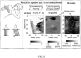
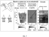
- Fig. 6 and Fig. 7 provide examples of the clinical applicability of embodiments of the present invention to tumor delineation and differentiation.
- In-vivo data were recorded at the University Hospital of Zurich for a female patient showing a cancerous lesion - which biopsy revealed as invasive ductal carcinoma ( Fig. 6 ), and a second female patient showing a benign lesion - confirmed to be a fibroadenoma ( Fig. 7 ).
- Conventional ultrasound B-mode images are provided for both lesions, both appearing as a dark region followed by a shadow region, which do not show a delineation and differentiation of the lesions in terms of gray level contrast.
- Multi-static data A(t, tx, rx) was acquired based on a commercial FDA-approved SonixTouch research ultrasound machine, from Ultrasonix Medical Corporation, Richmond, BC, Canada.
- the process is repeated for all transmitter elements, so that a total of N 2 time traces were recorded in ⁇ 0.1 s (about 100 MB).
- the displacement tracking (motion estimation) algorithm described in Eq T.1 was applied between beamformed images corresponding to increasing ⁇ pairs.
- a texture correlation block of 1x1 mm 2 (52x3 pixels 2 ) was used, with a search range of 0.125 us.
- a one-dimensional correlation search was performed in y , using a zero-normalized cross-correlation (ZNCCC) to find the vertical displacement ⁇ y in metrs at each point (x, y).
- Time measurements ⁇ m with correlation coefficients c yx ⁇ m , n opt ⁇ > 0.5 were discarded from the measurements.
- the "multi-angle anisotropically weighted total variation (MA-AWTV)" with three gradient (-22.5°, 0°, 22.5°) directions was used.
- the path lengths l p,c were calculated with linear interpolation.
- Figure 6 and Figure 7 show speed-of-sound images reconstructed with the SDR method.
- the measurement data ⁇ t shows large empty regions corresponding to the tissue regions no displacement information could be extracted. These were observed for instance in image areas not traversed by the plane wavefront, but also in the low echogenicity region observed around the breast lesions.
- any displacement tracking algorithm may show tracking failures, corresponding to image areas, where speckle information is not sufficient for extracting displacements.
- the presently suggested SDR reconstruction can handle these empty regions, allowing inputting incomplete tracked frames into the reconstruction.
- An FDR requires a complete ⁇ t measurement for all the tissue region.
- the combination of a large part of measurement data missing, together with the noise of the speckle measurements leads to a poor reconstruction, in which the tumorous inclusions cannot be delineated.
- the SDR reconstruction provides a clear delineation of the malignant tumor region, in agreement with the inclusion visible in the B-mode image.
- the sound-speed imaging allows for a sharp delineation of the tumor area where sound-speed changes occur, which is not possible in the B-mode images, due to the shadowing (increased acoustic attenuation) behind the lesions.
- Displacement estimation preferably is used in elastography, where local displacements are observed in response to some external excitation in order to estimate tissue viscoelasticity.
- Displacement tracking preferably is used in order to infer apparent displacements due to differences in speed-of-sound (SoS).
- SoS speed-of-sound
- the image processing and analysis techniques of optical flow and image registration may also be capable of finding displacements. This then allows for standard techniques, such as parametric (B-spline) or non-parametric displacement estimators, as well as using the consistency of displacement across several frames to increase accuracy and resolve ambiguities by removing outliers in displacement estimations.
- standard techniques such as parametric (B-spline) or non-parametric displacement estimators
- the ultrasound transducer may comprise a set of transducer elements each containing one emitter element and one receiver element, or a combined emitter and receiver element.
- the emitter elements of the set and the receiver elements of the set, or the transducer elements respectively are arranged in a straight row.
- the first direction of the gradients of the ultrasound parameters is a direction y orthogonal to a longitudinal extension of the set of emitter elements Tx and the set of receiver elements Rx, or the transducer elements respectively, and the second direction x is orthogonal to the first direction y.
- the emitter elements of the set and the receiver elements of the set, or the transducer elements respectively are arranged in a curved line, and preferably along a convex line.
- Each transducer element, or each emitter element and receiver element has a principal direction referred to as radiation axis along which the transducer element emits ultrasound.
- the first direction y of the gradients of the ultrasound parameters represents an average of the radiation axes of the set of emitter elements Tx and the set of receiver elements Rx, or the set of the transducer elements respectively.
- the second direction x is orthogonal to the first direction y.
- the second direction is defined by a maximum angle ⁇ max with respect to the first direction, which maximum angle ⁇ max is defined by a maximum inclination of the ultrasound beam or non-focused ultrasound wavefront transmitted by the set of emitter elements Tx and received by the set of receiver elements Rx, and a third direction preferably is defined by the negative maximum angle ( ⁇ max ).
- every transducer element may have a defined radiating axis y.
- several transducer elements together can allow angulation of the ultrasound transmission, for instance, by generating plane waves with a defined angle, or by generating a steered ultrasound beam.
- ⁇ max a maximum angle that preferably can be generated is referred to as ⁇ max which preferably is dependent on physical constraints as side lobes, or design decisions to use just a limited set of angles.
- Fig. 4 illustrates a block diagram of a medical ultrasound system according to an embodiment of the present invention, employing two different approaches in generating an ultrasound based tomographic image, and including one or more preferred buildings blocks already addressed in the previous sections.
- only one of the approaches of generating an ultrasound based tomographic image is implemented and is applied in a medical ultrasound system.
- ultrasound signal frames are generated from the tissue to be investigated in block 110, preferably by means of an ultrasound transducer.
- Each frame preferably represents an ultrasound wave received by one or more receiver elements of the transducer in response to an ultrasound wave emitted by one or more of the emitter elements of the transducer.
- Each frame, and hence each measurement preferably is taken from a different plane-wave angle, i.e. by holding the transducer in a different angle relative to the tissue to be investigated, such as is illustrated in Fig. 1 , for example.
- timing of the ultrasound signal frames corresponding to different paths through the tissue / angles of the ultrasound transducer is evaluated. For this purpose, displacement tracking is performed in block 120 for any frames corresponding to different measurement angles, however with a focus on the same location of the tissue.
- local mis-registration between two or more frames is performed in block 125. Based on such mis-registrations, represented e.g. by differences in the measurements in time, a spatial-domain reconstruction is applied in block 130, which effectively leads to a determination of a speed of sound distribution over the discretized tissue region, see block 135. The speed of sound distribution may then be graphically displayed as ultrasound based tomographic image.
- the ultrasound parameter to be determined per discretized cell of the tissue is not speed of sound but attenuation, instead. Accordingly, it is not timing information in the received ultrasound signal frames that is evaluated, but it is the amplitude or power of the ultrasound signal frames received, see block 140. Hence, an amplitude or power comparison is performed for any frames corresponding to different measurement angles, however with a focus on the same location of the tissue.
- local amplitude / power shifts are determined in block 145 for the respective signal frames.
- a spatial domain reconstruction is applied in block 150 providing an attenuation distribution over the discretized tissue region, see block 155. The attenuation distribution may then be graphically displayed as an ultrasound-based tomographic image.
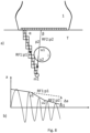
- FIG. 8 illustrates a method and a medical ultrasound system according to an embodiment of the present invention.
- the physical set-up of the medical ultrasound system of FIG. 8a is identical to the set-up shown in FIG. 1 .
- the ultrasound parameter extracted from the measurements is different: While in Fig. 1 , the ultrasound parameter investigated is speed of sound, in FIG. 8 , it is attenuation of the ultrasound wave. Accordingly, if put into context with the embodiment of FIG. 4 , the embodiment of FIG. 1 may represent a system / an approach including the upper branch of the block diagram of FIG. 4 , while the embodiment of FIG. 8 may represent a system including the lower branch of the block diagram of FIG. 4 .
- Fig. 8a again, two sample ultrasound waves are directed towards location m1 in the wave-plane.
- the waves are referred to as RF1 and RF2, wherein wave RF1 takes path p1 inclined by angle ⁇ with respect to the row of the elements of the transducer 1, while wave RF2 takes path p2 inclined by angle ⁇ with respect to the row of elements of the transducer 1.
- wave RF1 takes path p1 inclined by angle ⁇ with respect to the row of the elements of the transducer 1
- wave RF2 takes path p2 inclined by angle ⁇ with respect to the row of elements of the transducer 1.
- path p1 there is no inclusion
- inclusion i is traversed between locations u1 and u2.
- an envelope of the amplitude or power of the corresponding waves is referred to by RF1 and RF2 their travel through the tissue T. It can be derived, that wave RF1 not passing any inclusion is less damped than wave RF2 passing the inclusion i.
- a difference in the envelope of the amplitudes of the waves (such as received at the corresponding receiver elements) is referred to as shift in amplitude or power ⁇ a in FIG. 8b ), comparable to the difference of time of flight values for the embodiment of Fig. 1 . Accordingly, instead of a time difference between the time of flight values of two waves travelling different paths through the tissue resulting in the determination of speed of sound values for the individual cells, such as shown in FIG. 1 , now a difference between the amplitudes / powers of two waves - and more precisely of the two reflected waves as received by the receiver elements - allows for determining attenuation values for the individual cells according to FIG. 8 .
Description
- The invention relates to a medical ultrasound system and to a related method.
- Tumors and certain other anomalies in tissue are not always detectable in conventional B-mode ultrasound systems. However, these pathologies may present high contrast regarding other ultrasound characteristics, such as ultrasound propagation speed and attenuation. In order to obtain spatially-resolved images of these parameters, similarly to X-ray Computed Tomography (CT), ultrasound waves are transmitted through tissue and recorded at multiple angular directions, a family of methods known in the art as Ultrasound Computed Tomography (USCT). However, air (e.g., lungs) and bones behave as natural barriers to the propagation of ultrasound, limiting the applicability of ultrasound to soft tissue regions accessible from the skin (acoustic windows). Therefore, on the contrary of X-ray CT or Magnetic Resonance Imaging (MRI) full-body USCT is not feasible.
- Medical applicability of USCT is currently limited mainly to the breast. This presently requires high-end application-specific Ultrasound Computed Tomography (USCT) equipment, based on a large number of stationary ultrasound sensors positioned around the breast, see "Breast density measurements with ultrasound tomography: A comparison with film and digital mammography", Duric et al., Med. Phys. 40 (1), 2013, or by mechanically rotating ultrasound sensors around the breast, see "Imaging of Sound Speed Using Reflection Ultrasound Tomography", Nebeker et al. Ultrasound Med 2012, 31, pp 1389-1404, both of which systems require the immersion of the breast in water and scanning it with a bulky custom-made ultrasound system. Though accurate results, such systems are burdensome in daily clinical use, they require additional space in the clinics and specialized personnel to perform, and they are typically costly and are constructed highly application-specific, in contrast to typical ultrasound systems that allow for wide-range of clinical uses.
- In the method described in
WO 2015/091519 A1 a Frequency Domain Reconstruction (here abbreviated as FDR) is proposed. Particularly, the Discrete Fourier Transform (DFT) Δτ(kx,kz,ϕ,ϕ0 ) of the local echo phase shift Δτ(x,z,ϕ,ϕ0 ) between two directions ϕ and ϕ 0 over the image region (x,z) is calculated for determining the local sound speed c(x,z). Then, harmonic components (kx,kz) of the slowness σ(kx,kz ) are determined in the frequency domain using a relation equivalent to:
WO 2015/091519 : - The ill-posedness of the reconstruction results in low frequency artefacts that disturb the baseline of the bulk sound speed, as well as in high frequency artefacts that spread downwards through the image (page 22, Lines 14-17).
- With growing regularization of Tinv , artefacts due to the ill-posedness of the reconstruction are reduced, but "limited view artefacts", i.e. blurring of the upper and lower edges of the contrast regions and a drop of the base line adjacent to the left and right edges, become stronger, resulting in gradual loss of axial resolution, (page 22, Lines 17-25) .
- The local information can only be fully taken advantage of in the absence of noise when the regularization can be low. In practice, the local phase shift may be determined using echo phase tracking, which is prone to errors. With growing strength of regularization, the resulting image converges to an image with no axial resolution and with artifacts (page 23, Lines 12-13), (page 25, Lines 13-16).
- "Because of regularization, part of the spatial frequencies of the image are missing and the pixel gray level does not directly represent sound speed" (page 26, Lines 6-8).
- "The calculation of the calculation of the DFT requires that σ(x,z) is defined over the full image region (x,z). However, often in real tissue, strongly hypo-echoic regions such as large blood vessel lead to regions of missing data in the local echo phase shift maps, which, if not accommodated, lead to image reconstruction artifacts" (page 29 - Line 16-19) .
- An in-depth analysis of this method associates the observed artefacts to an inappropriate regularization strategy, which limits the axial resolution, see "Computer ultrasound tomography in echo mode for imaging speed of sound using pulse-echo sonography: proof of principle", Jaeger et al. 2015, Ultrasound in Med. & Biol., Vol 41, No. 1, pages 235-250. The phase noise after sound-speed reconstruction results in a regular structure of high-spatial frequency streaks that run diagonally through the image, which is the main cause of loss of contrast in cases of low regularization. The regular structure of the image noise indicates that it is produced by an inappropriate regularization strategy.
- In addition, document
US 2002/0099290 A1 discloses A system and method for doing both transmission mode and reflection mode three-dimensional ultrasonic imagining. The multimode imaging capability may be used to provide enhanced detectability of cancer tumors within human breast, however, similar imaging systems are applicable to a number of other medical problems as well as a variety of non-medical problems in non-destructive evaluation (NDE). - The invention is defined by the
independent claims 1 and 27. - The problem to be solved is therefore to enable a widespread use of ultrasound computed tomography (USCT). This problem is solved by an ultrasound transducer for emitting and receiving ultrasound, which ultrasound transducer is electrically connected to a processor. The processor is configured to determine an ultrasound based tomographic image subject to ultrasound waves received by the ultrasound transducer in response to ultrasound waves emitted by the ultrasound transducer and scattered and / or reflected by tissue to be investigated.
- Hence, a single-sided inspection of an organ and/or tissue structure accessible is provided with conventional ultrasound. Single-sided means that the ultrasound transducer that preferably is a hand-held represents the sole ultrasound emitting and receiving entity, such that tissue to be investigated is approached by the ultrasound transducer from one side only. Preferably, the ultrasound transducer has a common housing for a set of emitter elements and a set of receiver elements for emitting and receiving ultrasound waves respectively. In particular, there is no man-made reflector involved in the measurements. Instead, the emitted ultrasound waves are scattered and / or reflected by tissue to be investigated, and in particular by structures in the tissue such as inclusions which represent one of spots or regions in the tissue with different ultrasound transmission characteristics than other regions in the tissue. Accordingly, it is preferred that the proposed system operates without any reflecting means other than the tissue itself.
- Preferably, a novel image reconstruction method is applied, which can be built upon conventional hand-held ultrasound hardware. The minimum hardware required for implementing this method is the ultrasound transducer capable of emitting ultrasound waves and receiving and preferably recording ultrasound waves reflected and/or scattered at tissue structures, and the processor.
- Preferably, the reconstruction method executed by the processor is based on misalignments in ultrasound parameters between images taken from different angles between the ultrasound transducer and the tissue to be investigated. Such misalignment, also referred to as mis-registration, in the ultrasound parameter, such as speed of sound, may be found in one or more or all areas of the investigated area of the tissue, each area referred to as cell, which cell is exposed to at least two ultrasound waves emitted from different angles. Preferably, in exposing the area of tissue to be investigated to ultrasound waves from different angles, paths of the ultrasound waves travel through at least partly different regions of the investigated area. Preferably, the regularization comprised in the reconstruction step is applied directly on the ultrasound parameters determined for each spatial region, i.e. cell, for the tissue, which spatial region preferably is a discrete area. Preferably, a spatial domain reconstruction is applied for image generation based on the mis-registrations detected and / or computed in the discretized problem space of the tissue.
- For a single measurement from one angular direction with respect to the tissue, it is preferred to emit an ultrasound wave by one of the emitter elements, and receive and record the scattered and / or reflected ultrasound wave by all the receiver elements.
- According to an aspect of the present invention, an ultrasound image reconstruction method is proposed, wherein a plurality of ultrasound signals is collected to allow access to set of cells in the imaged domain from paths passing through different domain regions, wherein the local mis-registrations between these plurality of ultrasound signals are determined, and wherein a spatial-domain reconstruction is employed based on computed mis-registrations in a discretized problem space.
- Preferably, a system of equations is solved which relates to a discrete set of time measurements with speed of sound values in a discrete number of cells.
- Preferably, the time measurements are expressed by a linear combination of the speed of sound values in the discrete number of cells.
- Preferably, a system Δt = Lσ is solved wherein the weighted path lengths are assembled in a matrix L of dimensions [MxC] and wherein the matrix L represents geometric information that depends on the transmitter-receiver setup of the transducer and the size and shape of the cells, in particular their granularity/resolution. The speed of sound values per cell c are preferably assembled in the vector σ of dimensions [Cx1], and the time measurements τm in the vector Δt of dimensions [Mx1]. The overall number of time measurements M preferably is equal to or larger than the number of cells C for a determined linear system.
- Preferably, prior physical information is incorporated, such as iteratively compensating wave refractions, wave path uncertainties, or others, preferably with a scheme in which the path measurements are iteratively actualized.
- Preferably, prior information about lesion, aka tissue structures, is incorporated, such as location, size, delineation. For instance, a single speed of sound value is determined for a lesion region and a background region outside the lesion region each.
- Preferably, acquisition of multi-static data is applied (every single element transmits sequentially, and all receiver signals are acquired), from which different path measurements can be generated (plane wave, synthetic aperture, focused...) .
- Preferably, quantitative reconstruction is applied including procedures for estimated background speed of sound value and the quantitative speed of sound contrast in the inclusions. Preferably, observed timing differences with respect to an initial assumed speed of sound estimate may allow estimating these values.
- A USCT method is proposed, which only requires single-sided access to the tissue to reconstruct ultrasound acoustic properties, and can preferably be implemented on a conventional medical ultrasound array, i.e. the ultrasound transducer, which can be hand-operated by a sonographer. Preferably, by combining different ultrasound transmitter excitations with image registration techniques, for instance speckle tracking, followed by a novel spatial domain reconstruction, local variations of speed of sound (SoS) in the tissue can be imaged.
- The method is well suited to image organs in which only single-sided access is possible, such as liver, kidney, etc. However, it also significantly simplifies the clinical workflow for organs in which double-sided access is possible, in particular the breast, since no water bath, additional hardware elements are necessary to reconstruct USCT parameters.
- The medical ultrasound system is used in a medical context: The medical ultrasound system may be used for one or more of medical screening, diagnosis, staging (e.g. of cancer), preoperative planning, intra-operative guidance, and post-operative follow-up.
- Preferably, the ultrasound transducer is hand-held which is meant to be portable, or mobile. The ultrasound transducer can be held by a sonographer such as a doctor or a nurse during inspecting a patient.
- The medical ultrasound system preferably is characterized by a Spatial Domain Reconstruction (SDR), for which time measurements are received and / or recorded by the ultrasound transducer for specific ultrasound wave propagation paths traversing a set of discretized tissue cells. Preferably, speed of sound variations in each of these cells are calculated from discretized relations between the speed of sound increments in individual tissue cells and the cumulative time measurements recorded by the transducer, given defined propagation paths. Thus the relations are defined and solved directly in an arbitrary spatial grid. With respect to previous art the following advantages are obtained:
- Spatial regularization can directly be applied in the spatial domain to solve the inverse problem, which allows for introducing available prior information about the reconstructed sound-speed distributions. For instance, it is possible to find the solution amongst the set of possible solutions that provides the best geometric delineation of inclusions (portions of the tissue that may be considered as tumorous), and the best accuracy for the sound-speed values in the inclusions. For instance, if the position and geometry of inclusions are a priori known (from instance from an ultrasound B-mode image), a reconstruction can be defined which determines the best sound-speed values in the inclusions.
- Quantitative speed-of-sound images, for example, are obtained in m/s, which provide a quantitative biomarker for tissue diagnosis and differentiation.
- The inverse problem can be solved, even if time measurements are only available for partial regions of the tissue domain and a harmonic decomposition of the image cannot be calculated. Similarly, the reliability of time measurements at specific tissue structures, for instance, expressed in terms of a correlation coefficient, can be directly incorporated into the regularization of the inverse problem.
- Arbitrarily complex path geometries can be easily incorporated with simple relations (scaling and additions), which allows defining arbitrary measurement configurations and correcting for physical effects such as wave refraction.
- Other advantageous embodiments are listed in the dependent claims as well as in the description below.
- The embodiments defined above and further embodiments, features and advantages of the present invention can also be derived from the examples to be described hereinafter and are explained with reference to the annexed drawings, wherein:
-
FIG. 1 illustrates a measuring scenario including a medical ultrasound system according to an embodiment of the present invention; -
FIG. 2 illustrates preferred strategies for the definition of a set of wave propagation paths p, from which time measurements τm can be extracted, according to embodiments of the present invention; -
FIG. 3 illustrates different measurement approaches according to embodiments of the present invention; -
FIG. 4 illustrates a medical ultrasound system according to an embodiment of the present invention; -
FIGs. 5 to 7 shows measurement results of a medical ultrasound system according to an embodiment of the present invention; -
FIG. 8 illustrates a method and a medical ultrasound system according to an embodiment of the present invention. - In a generic implementation of a medical ultrasound system illustrated in
Fig.1 , anultrasound transducer 1 emits and receives ultrasound waves along a total of P wave propagation paths p, corresponding to predefined trajectories, along which ultrasound waves propagate. Accordingly, the time delay tp is measured in form of a time difference between the time of emission of the ultrasound wave by one or more elements Tx of a set of emitter elements of theultrasound transducer 1, and the time of receipt of the reflected ultrasound wave by one and preferably more and preferably all of elements Rx of a set of receiver elements, that may preferably be arranged in a row in thetransducer 1. Thetransducer 1 accesses tissue T for investigation. This time delay tp is also referred to as time of flight. For tissue structures mx, either of natural or artificial nature, for which the position and/or geometry is accurately known, tp can be measured in absolute terms. In general, if the actual position of the tissue structures cannot be accurately determined, relative measurements τm can be obtained, which compare the time of flight along a predefined set of N paths {pm }={p 0 ,p 1K pN }, with N ≤ P.
- The weights wm,p typically take the values +1 or -1 to express a relative measurement. Paths p which are not part of the measurement m are zero weighted.
- For instance, in the most simple version two distinct paths j (test) and i (reference), are compared for each measurement, in which case

- In this case, wm,p = 1 for p = i, wm,p = -1 for p = j, and wm,p = 0 otherwise.
- Preferably all paths converge to the same point or region in space.
- Consequently, the same tissue position x,y preferably is accessed from two different wave propagation paths p1,p2 corresponding to two different angles θ1, θ2. The relative time measurements _m at coordinate x, y are preferably obtained from a timing shift observed in the images seen from these two angles, i.e. in the ultrasound waves received.
- Preferably, a spatially-resolved speed-of-sound (SoS) image is determined based on multiple time measurements as expressed by Eq. D.1.
- For this purpose, the tissue region insonified by the transducer is discretized into a finite number of cells c that reflect locations in the tissue. Without loss of generality, for a two-dimensional ultrasound system, for instance, it is preferred that a linear or a convex array of emitter and receiver elements is used so that the wave propagation is referred to a single plane defined by the radiation axis of the emitter and receiver elements, collectively referred to as transducer elements, and the tissue region is defined by one plane, in which the cells are located. The plane is then discretized into cells traversed by the paths p.
- This cell structure supports the localization of portions / structures m of tissue that may be considered as tumorous, which portions are also referred to inclusions. The cell size is to be defined upfront and determines the resolution of the image. The process of determining the ultrasound parameter per cell based on the time of flight values is also referred to as reconstruction. Finally, a
processor 51 of the medical ultrasound system is configured to convert the ultrasound parameter values as determined into an image that preferably is shown to medical personnel on a screen of the system. The conversion may include a coding of the ultrasound parameter values into colors, for example, or into grey scales. - With a path length lp,c [m] per ray path p and cell c from the transmitter Tx to the reflecting structure m and back to the receiver Rx, the time of flight values tp are calculated in function of speed sound (SoS) increments σc -also referred to as slowness increments, per cell c, i.e.:

- This equation illustrates the time of flight values tp for a certain path p as a sum of individual speed of sound values σc per cell c, for the number of cells C that are travelled along the subject p path with the portion of the path length lp,c per individual cell c. Substituting Eq. D.3 in Eq. D.1 the relative time measurements τm are expressed in function of σc :

- The last equality merges the path lengths lp,c and measurement weights wm,p in a single linear combination of weighted path lengths Lm,c , which is summarized with a matrix L.
- The overall number of time measurement M preferably is equal to or larger than the number of cells C for a determined linear system. The system represented by equation D.4 can be expressed in matrix form for all measurements M and discretized cells C as Δt = Lσ, wherein the weighted path lengths are assembled in a matrix L of dimensions [MxC] and represent geometric information that depends on the transmitter-receiver setup of the transducer and the size and shape of the cells, in particular their granularity/resolution. The speed of sound values σc per cell c are assembled in the vector σ of dimensions [Cx1], and the time measurements τm in the vector Δt of dimensions [Mx1].
- In a first approximation, the path lengths lp,c for each ray path p are calculated as the segment length traversing the cell c (
Fig. 1 ). For those skilled in the art, interpolation strategies are available, which can be utilized to improve the ray path representation on a discrete grid. These include nearest neighbor interpolation, linear interpolation and higher order interpolation kernels. By adding a certain kernel function or smoothness function to describe pressure distribution across the ray cross-section, the consistency and stability of the solvers is known to be enhanced. These kernel functions may be position dependent and obey both physical and computer graphics considerations. - The inversion of Eq. D.4 requires the acquisition of relative time measurements τm which incorporate paths with respect to tissue structures, which can be identified in the ultrasound data. The recorded ultrasound signals can be described as a superposition of echoes at reflecting tissue structures m1, m2, ... In the most simple description, each echo is a delayed ultrasound wave. So if the echo corresponding to the same tissue structure can be identified for two different wave propagation paths, the relative time measurement τm can be obtained.
- In a possible scenario, a series of echogenic features are identified in the recorded ultrasound signals. These can for example include natural geometric features (vessels, air/bone interfaces) or artificial features (microbubbles, catheters, biopsy needles, embedded reflectors). If the position and geometry of these features are well-defined, the problem reduces to a tracking problem, from which absolute time measurements can be obtained for each path. If the position and geometry of the reflecting features is not accurately known (for instance, due to the unknown speed-of-sound distribution), relative measurements that contain the same feature can still be obtained along different wave propagation paths, which is known in several contexts by "multipath" or "spatial diversity". Image registration procedures well known in the literature can then be applied to align the reflectivity patterns obtained from different path directions. The local mis-registration residuals provides relative time measurements for these paths.
- In another possible scenario, which is preferred for soft tissue (for instance breast, liver, muscle, myocardium), the recorded ultrasound signals comprise of a superposition of a larger number of microscopic features (for instance, individual tissue cells), which converge into homogeneous textured patterns or speckle, typically showing Rayleigh distribution. Each tissue region is known to show a unique speckle tracking. Speckle tracking (ST) algorithms are well-known in the ultrasound elastography literature, which provide "best texture match" between two displaced / scaled / rotated versions of the same speckle patterns, allowing to determine displacements in the echo signals. Some well-known algorithms are Digital Image Correlation and Optic Flow. These algorithms allow the registration of speckle patterns obtained from different path directions.
- In a preferred version, which is implemented for the illustrated examples, a correlation measurement is defined between two different speckle patterns:


- The displacement measurements n opt obtained at different tissue positions m, scaled in time units, provide a set of time measurements τm which can be used as input data for equation Eq. D.4.
- Eq. T.1 may be extended to signals of higher dimensional order x[m1, m2...], y[m1, m2...], for which higher order correlations are performed. For instance (as exemplified below in
Figure 6 andFigure 7 ), two-dimensional correlations may be performed by simultaneously considering ultrasound signal traces corresponding to adjacent receiver elements or by considering adjacent beam formed lines. - A quality measurement qm for the registration, can be obtained at each m by calculating


- Even if time measurements are not available in a wide range of tissue cell positions m, speed of sound values can still be reconstructed for these cells c, as long as sufficient measurements are available for a determined system Δt = Lσ. This is illustrated with an example in
FIG 1 . Even if the measurements m1 and m2 are obtained outside the tumorous inclusion region, the compared paths {p1, p2} for m1 traverse the inclusion and allow differentiating it with respect to m2 {p3, p4}, where the inclusion is not insonified. This is an important advantage of the presented invention with respect to prior FDR art, in which time measurements m1, m2 are required at all calculated cell positions c1, c2 to be able to perform a harmonic decomposition of σ. - In a more general scenario the quality measurement (negative values are zeroed) or a transformation of it can be incorporated into the solution term Eq D.4 to regularize the solution term. For instance, if the optimum solution is expressed as a minimization process


- The simple texture matching described here can be generalized to incorporate regularization information, for instance, physical and geometric constraints given by the way the matched patterns are generated (see next section) or continuity constraints. The registration can then be defined as an optimization problem based on the minimization cost function, which simultaneously incorporates the information of all measurements m. Such cost can also be minimized using discrete and graph-based optimization techniques well-known to those skilled in the art, such as graph-cuts, Markov-random Fields, and Conditional Random Fields. Outlier detection algorithms, for instance Random sample consensus (RANSAC) can be used to filter out undesired structures from the time measurements. Texture matching redundancies between different path combinations may also be exploited to improve speckle tracking quality.
-
Figure 2 exemplifies preferred strategies for definition of a set of wave propagation paths p, from which time measurements τm can be extracted according to some of the methods outlined above. Even if the Spatial Domain Reconstruction (SDR) allows for arbitrary path comparisons, certain path properties are preferred. Sufficient diversity should be provided to solve the inverse problem Eq T.3. For instance, it is well-known from the theory of computed tomography reconstruction that the conditioning of the reconstruction improves if the reconstructed cells are traversed by a wide range of path directions. The defined paths preferably highlight the matched tissue features or patterns, so that accurate measurements qm can be obtained in the registration step. Incremental differences between paths are also more bound to provide a good matching quality than larger differences. An organized path definition in function of a few simple parameters θi - i.e. the angle of the path in the plane e.g. relative to a longitudinal axis of the ultrasound transducer, or relative to a horizontal axis of the ultrasound transduced , e.g. represented by a linear row of transducer elements - that can be adjusted in the ultrasound transducer is also desired to simplify the measurement process, as well as to optimize measurement speed. - In a preferred embodiment, a single transducer with N transducer elements is operated in "multi-static" or "full matrix" mode, with each element individually firing and the rest receiving. This concept is equivalent to ultrasound imaging with transmitter and receiver aperture of one element. This provides a total of N × N time traces for the transducer and provides the most generic representation of a linear tissue model. The multi-static matrix can be represented as A(t, tx, rx), where t is the time coordinate, and tx and rx are respectively the transmit and receive indexes. The firing process can be optimized for real time operation, for instance, by simultaneously recording all receive channels rx for each firing element tx. The signal to noise ratio can be also be optimized by coding the signals before transmission. The coding can be performed in either or both time and spatial domains, and allows to measure the multi-static matrix with significantly improved signal to noise ratio.
-
Figure 2 illustrates several examples of path definition strategies. Non-focused wavefronts can be generated to achieve a large tissue coverage in front of theultrasound transducer 1. Non-focused wavefronts are plane wavefronts or full aperture wavefronts, which are shown inFig. 2a as white areas embraced by a dashed area representing areas not exposed to the ultrasound wavefront, and synthetic aperture or single-element circular wavefronts are shown inFig 2b by means of an arrow. - In the case of plane wavefronts (
Fig. 2a ), spatial diversity can be obtained by controlling the angle of incidence θ of the plane wavefront. Consequently, the same tissue position m can be accessed from two different wave propagation paths (p1, p2) corresponding to two different angles (θ1, θ2) and a time measurement τm can be obtained by subtracting the time difference between the two paths p1, p2. Plane wavefronts are synthesized by firing all elements of the ultrasound transducer (full aperture) with controlled transmit delays between transmit elements to achieve a coherent wavefront. For instance, for a linear array of transducer elements with element separation pitch as pictured inFig. 2a and a plane wavefront of angle Θ1, the transmitter delays for element index tx are adjusted as:

- It should be noted that, due to their angulation, plane wavefronts provide only limited coverage of the tissue domain. The dashed regions in
Fig. 2 are "shadow regions", which are not accessible by the plane wavefront. If two such plane wavefronts Θ1 and Θ2 are compared to obtain a time measurement at point m, such point m preferably is within the coverage region of both plane wavefronts. - Circular wavefronts can be generated by firing one element at a time (
Fig. 2b ). In this case a full coverage of the tissue region in front of thetransducer 1 is obtained while typically there is no shadow region in the tissue. In this case, the same transmit delay can be applied for all transmit elements. Spatial diversity is obtained by comparing two paths p1 or p2 of circular wavefronts generated by two different transducer elements T1 and T2 representing respective paths p1 and p2 with corresponding angles Θ1 and Θ2 with respect to the same tissue position m. - Clutter may complicate time measurements τm if the matched tissue structures are overlapped with echoes from other reflecting tissue structures, which coincide with the reflections of these structures. This problem can be addressed by collimating the transmitted ultrasound energy in a localized beam that propagates only through a defined region of the tissue. For the plane wavefronts described in
Fig. 2a this can be achieved by limiting the aperture of the transmitted plane wavefront, as it is illustrated inFig. 2c . A natural collimation of the plane wavefront is obtained at the near field distance NF = Aperture2 /4/vB*freq, where the Aperture is expressed in distance units [m], and freq is the frequency of the transmitted ultrasound pulses. Starting from the multistatic matrix A(t, tx, rx) and applying Eq. P.1 for limited apertures, collimated wavefronts can be obtained at arbitrary tissue positions. Collimation as well reduces the extent of "shadow regions", especially in the region close to the transducer emitting surface (near field). - Another possibility to reduce clutter is to generate a focused ultrasound beam at defined measurement points m, so that tissue reflectivity is maximized in a small region around the desired measurement point m. In this case the time delays of the transmit elements are adjusted to achieve a constructive interference at the position m: delay(tx) = -distance(tx, m)/vB, where distance(tx, m) is the geometric distance between the transmit element Tx and the measurement point m. Spatial diversity can in this case be achieved by synthesized focused ultrasound beams with different steering angles Θ1 and Θ2, as illustrated in
Fig 2d . Focused ultrasound beams at an arbitrary tissue position can be generated from the multistatic matrix A(t, tx, rx) by applying Eq. P.1. with the aforementioned delay(tx). A full aperture of finite size can be used to generate focused ultrasound beams. Undesired physical effects, such as side-lobes or near-field interferences, can be minimized by ensuring a constant ratio #f =depth/aperture, or by scaling the signals of the transmit aperture with an apodization function apodization(tx), for instance a Hanning, Hamming or Gaussian window. Apodization can also be applied to the collimated plane wavefronts described inFig. 2c . - Circular wavefronts with increased signal to noise ratio may also be generating by firing multiple elements at a time, and combining their contributions with Eq. P.1. This concept is known to those skilled in the art as "virtual sources". The center of the circular source is in this case defined by focusing the ultrasound waves at a position m in front or behind the transducer radiation surface. The same mechanism may be used to achieve collimated sources in the transducer elevation plane. In general, several techniques are known for improving the signal to noise ratio by firing multiple elements with different transmit pulses, for instance, by using different delays, apodizations (including positive/negative/zero- sign), or different pulse functions.
- So far, spatial diversity and clutter reduction have been described in terms of the ultrasound transmit process. However, the ultrasound receive process can also be controlled to provide additional spatial diversity and clutter reduction. This is illustrated in
Fig. 2e . Similarly to Eq. P.1., by delaying and summing the ultrasound signals recorded by individual receiver elements, focusing and steering with respect to specific points m are achieved. Eq P.1 is then generalized as Eq. P.2:
- Eq. P.2 computes tissue reflectivity patterns for a set of measurement points m in function of diversity parameters defined in transmission θtx and reception θrx. Each B(m) can be understood as a beamformed ultrasound image. If an additional demodulation process is applied to B(m), it results in a so-called conventional ultrasound B-mode image. Therefore, ultrasound B-mode images obtained in function of different diversity parameters θ can be registered to obtain relative time measurements τm and subsequently to reconstruct the speed of sound distribution with Eq. D.4. However, in general, beamformed ultrasound images (radio-frequency RF or demodulated IQ data) are preferred, since the phase (time) can be tracked more precisely from the carrier frequency.
- If the speed of sound distribution is constant at all inspected tissue regions and the average speed of sound vB is accurately known, then all B(m,θtx ,θrx ) provide the same image B(m,θtx,θrx )=B(m). If this is not the case, small mis-registrations are observed between the images B(m,θtx,θrx ), which can be determined with the matching algorithms described in the previous section. Expressed in time units, the misregistrations (apparent motion / displacements) between two arbitrary images B(m,θ 1) and B(m,θ 2) provide relative time measurements τm , which enable the reconstruction of the speed of sound perturbations σ c at each cell with respect to the assumed nominal values vB.
- Given a recorded multi-static matrix and sufficient computational resources, all techniques described above can be applied to the multi-static matrix A(t, tx, rx) to obtain a large number of time measurements τm , which can be then used to solve the unknown speed of sound distribution from Eq. D.4. Following the synthetic aperture concept illustrated in
Fig. 2b , the theoretical maximum number of diversity paths for a given measurement point m, assuming that the point can be resolved, is given by the number of recorded transmit-receive combinations NxN. The maximum number of measurement points m over a defined tissue region is given by a discretization of the tissue region by the best achievable spatial resolution with ultrasound waves, which is typically an order of magnitude larger than the wavelength lambda = vB/f, with f being the dominating frequency of the ultrasound signals. This as well corresponds to the best spatial resolution of the cells c for the reconstructed speed-of-sound distribution σ. Therefore, a maximum of NxN measurements is theoretically available for each cell c, which provides a highly overdetermined system Eq. D.4, in which robust reconstructions can be achieved. - Three-dimensional reconstructions can be achieved for 2D-matrix array probes, other transducer constructs with more than one element placed or imaging in the out-of-plane direction. These allow for an extension of the spatial diversity strategies outlined in
Figure 2 . For instance, arbitrarily oriented plane wavefronts can be obtained (both in plane and out of plane inclination). Both spherical waves (single element fired) and cylindrical waves (a row or columns of elements simultaneously fired) can be used for spatial diversity. Similar considerations to those above regarding the maximum number of diversity paths apply. - In one example, relative time measurements m are performed at each cell c by comparing plane wavefronts at angles_θ1=20° and -20° with respect to_θ2=0°. Preferably, the_τm values were generated using a ray tracing algorithm, so that no uncertainties due to speckle tracking or unaccounted wave propagation paths are present. Random noise was then added to the _m matrix, following a Gaussian distribution with zero mean and a standard deviation expressed as percentage with {1,2,5,10,20,50,56,63}% of the peak_τm value for each example, which correspond to a signal-to-noise ratio of {τ40,34,26,20,14,6,5,4} dB.
- Physical wave propagation trajectories can be incorporated in a straight forward way to the Spatial Domain Regularization (SDR). An example is shown in
Figure 3 . In a first iteration, a homogeneous background is assumed as prior information and straight ray tracing is used to calculate a speed of sound image. This first image can be used in a second iteration to compute more realistic ultrasound propagation paths in order to improve the beamforming and reduce clutter in the speckle tracking. Moreover, the prior information can be introduced into the spatial regularization, allowing for adjusting the wave propagation paths to describe the actual wave trajectories under consideration of wave refraction effects. This process can be iteratively repeated until a convergence is obtained. Moreover, the full wave equation can be simulated for the prior configuration and a time surface can be computed for each tissue position, from which the gradients determine the possible ray trajectories at all points. It is also possible (time reversal physics) to reverse the wave propagation of received signals through a simulation model - with or without prior inclusion information-, to achieve convergences at originating scatter sources. Overall all these strategies can be used to improve the image contrast and resolution and the speckle tracking accuracy. - Finding σ, which contains the slowness σc values per cell c, is the inverse problem:

- The resulting matrix σ hence represents the speed of sound distribution across the cells c, i.e. for the virtual cells the tissue T in the subject plane is divided into, and in particular the cells c that are affected by an inclusion m, see e.g.
Fig. 1 , given that the speed of sound in such cells is different to the speed of sound in cells that cover non-tumorous tissue. - It is preferred, that for identifying a cell c in the plane, Cartesian coordinates x and y are used, preferably in an orientation with y normal to the transducer surface in the center, also referred to as vertical direction, and x orthogonal to that, also referred to as horizontal direction. The indices i and j are then respectively used to enumerate cells in x and y directions. For 2D matrix array transducers, trivially a 3rd axis z orthogonal to the other two axes can be introduced in order to generate a 3D cell grid for reconstructions in 3D domain.
- In a preferred implementation, the quantitative speed of sound values are directly calculated from the slowness values as:

- In another preferred implementation, both the delays Δtp and slowness increments σc , as written in equation S.1, represent perturbations caused by inclusions with respect to homogeneous tissue, that is, a tissue model in which no inclusions are present.
- Preferably, a pre-step is then used to estimate the average speed of sound vB out of the measured time delay matrix. tp then corresponds to the delay residuals after subtracting from tp the delays caused by the homogeneous tissue, that is,

- Quantitative speed of sound images v[m,s] are calculated from vB and the slowness increments σ [s/m] for an individual cell c addressed by coordinates x and y in the plane

- A first estimate of vB is obtained from the known tissue type (for soft tissue the nominal value is 1540 m/s). Several global optimization methods are known in the literature to estimate vB to an accuracy of approximately 1%, for instance, by iteratively adjusting vB until the smearing of speckle patterns is minimized. Also the time measurements obtained for certain diversity configurations will show systematic baseline patterns if the wrong vB is used. Analysis of such patterns can be used to further refine the value of vB. An example is shown with Eq. E2.
- Therefore, it is desired to solve an incomplete reconstruction problem according to equation (Eq. S.2), which is inherently ill-posed. This means that the corresponding mathematical equations cannot be solved uniquely. Several potential solutions for the speed of sound matrix σ, or more general for the ultrasound parameter matrix, are possible. However, in solving equation (Eq. S.2) it is preferred and desired to find the solution amongst the set of possible solutions that provides the best geometric delineation of inclusions, and the best accuracy for the sound-speed values in the inclusions. However, the set of possible solutions is not to be determined: It is sufficient to determine the solution out of the set of possible solutions without the need to know these other possible solutions.
- Preferably, this optimization approach is implemented by:

- Therefore, it is preferred that mathematical regularization is introduced to obtain numerically bounded solutions, which allow for satisfactory reconstructions of the position and geometry of one or more tumorous inclusions in a homogeneous tissue background.
- In a first embodiment, a regularizing assumption is introduced for the smoothness of the SoS-image according to:

- Accordingly, not only the error function Δt-L*σ is minimized but a sum of the error function and an additional term D*σ. D is a gradient matrix introducing which cells are adjacent to each other, and, correspondingly, D*σ denotes the gradient of the speed-of-sound σ of adjacent cells in the plane. The usage of the term D*σ is based on the insight that desired solutions of equation Eq. S.2 show one or more closed inclusion geometries in a homogeneous tissue background. Hence, out of the set of possible SoS values solving the equation Eq. S.2, those are selected, that at least in combination with minimizing the error function with piece-wise constant cell values with sudden transitions where necessary.
- However, in another embodiment, D can be any other related property, such as curvature matrix (to regularize 2nd order derivatives), DFT/DCT to regularize frequency components, or any wavelet transform, etc. Hence, the ultrasound parameter values can be dependent on "other linear combinations" D, such as curvature, discrete Fourier/cosine transform, wavelet transform, of the ultrasound parameter values, and thus their derivatives.
- In a preferred embodiment, ∥Dσ∥ n minimizes a sum of horizontal and vertical gradients of the reconstructed image, and λ is a constant.
- The norm n of the smoothness term D*σ critically influences the reconstruction results. For example, if the L2-norm (n=2), which is defined for an arbitrary vector xq as ∥x∥2 = Σ q (xq )2, is applied to D*σ, a closed linear solution (Tikhonov regularization) of equation Eq. S.5 can be found, but smooth gradients are favored with respect to sharp gradients. Large jumps in the SoS values of adjacent cells, which may contain different tissue, are penalized unnecessarily with the L2-norm, creating unrealistically smoothed results.
- However, if the L1-norm n=1 is used ∥x∥1 = Σ q |xq |, which in the context of regularization is also referred to as total variation (TV) regularization or compressive sensing, sharp and smooth gradients are equally weighted, which leads to the reconstruction of piecewise homogeneous regions. With n=1, equation Eq. S. 5 becomes a convex problem, in particular a Second Order Cone Programming problem, which preferably is iteratively solved, with optimization methods such as the Interior Point Method and Alternating Directions Method of Multipliers (ADMM).
- According to various embodiments of the present invention, the regularization term that preferably contributes to the optimization can be calculated by one norm which shows TV behavior, such as L1-norm, see Eq. S.6, or L2,1-norms, see Eq S.7:


- Generally, in such grid-like organization of cells in the plane, where cells are arranged next to each other in rows in the horizontal direction as such forming columns of cells in the vertical direction, each cell has at least one neighbor in the horizontal direction and at least one neighbor in the vertical direction. Hence, such regularization term introduces directional gradients, and specifically gradients along the x-axis and another gradient along the y-axis. The indices i and j of each cell c refers to a position along the x and the y-axis respectively. The resulting SoS based image successfully filters out limited-angle artifacts and delineates closed inclusion geometries. Accordingly, the amount of information available in each angular direction is incorporated into the smoothness reconstruction.
- As laid out above, missing angular orientations owed to the non-360° setup of the transducer lead to distortion in the reconstructed SoS image. However, it is known up-front which angular orientations are available for each cell, since the wave propagation / ray paths are defined by the hand-held apparatus, apart from small perturbations introduced by tumorous inclusions. Hence, it is very preferred to weight the SoS gradient contributions in different angular directions, and preferably according to the availability and / or impact of ray information in each of these directions. The resulting regularization may be referred to as "Anisotropically Weighted Spatial Regularization". In a specific embodiment, this concept is combined with the total variation approach and is referred to, in the following, as "Anisotropically Weighted Total Variation" (AWTV).
- Hence, in a most basic form for two directions such as the orthogonal directions x and y referred to above, a constant κ is introduced in the regularization term as weight, which balances horizontal and vertical gradients according to the available ray information in each direction:

- This can similarly be achieved for equation S.7 by weighting axial components differently by parameter κ. Note that non-axis-aligned weighting can also be achieved by projecting derivative components in equations S.6 and S.7 onto tensors, although we herein prefer axis-aligned weighting. The weight κ can be tuned for each individual cell c. However, in a preferred embodiment, a single value κ is defined for the full image, i.e. the same weight κ is applied to all gradients of the one axis while the weight 1-κ is applied to all gradients of the other axis y. Under the assumption that κ ≠ 0.5, the gradients along one of the directions / axis are emphasized over the gradients along the other direction / axis. In a very preferred embodiment, κ=0.9.
- In another embodiment, the gradient directions used in the regularization is not limited to orthogonal directions. More than two gradient directions can be introduced in the spatial regularization term, which then may be referred to as "Multi-Angle AWTV" (MA-AWTV):

- Given the maximum available angle θ max the gradient directions α for a total of Nα different directions are preferably chosen as follows:

- 1) Initialize weights κα ={0};
- 2) For each wave path p crossing cell c:
- a. calculate the inclination of the wave path θ;
- b. Increase the weight κ α of the closest gradient direction {α} with respect to φ by the geometric overlap of path p with cell c. If θ > θmax , do not increase κα ;
- 3) Average {κα } over all cells.
- Note that not including the directions outside the imaging angular span [-θ max,θmax ] effectively assigns them no regularization. This avoids over-constraining directions, for which no boundary information is available, which reduces image artifacts. For conventional medical ultrasound arrays, θ>30° leads to strong grating lobes and cluttering and are typically not used.
- For plane wave emissions as illustrated in
Fig. 2a , the maximum angle θ max is obtained as the maximum plane wave inclination. For other path/diversity configurations a different subset of angles may provide better results. - If step 3 is omitted, cell-specific κ α values can also be used. In a preferred embodiment, three gradient directions are used, preferably: [0,θ max,-θ max], wherein 0° is defined as first direction y along the y-axis, i.e. orthogonal to the second direction along the x-axis defined by the longitudinal extension of the transducer.
- In a preferred embodiment, equation S.5 specifically is embodied as:

- In a different embodiment, equation S.5 specifically is embodied as:

- And in a further embodiment, equation S.5 specifically is embodied as:

- To keep the same regularization constant for equation S.11 and equation S.12, the weights are preferably normalized such that Σ α κ α = 1.
- It is also possible to use L2,1-norm of Eq. S.7 for the error function term, ∥Δt-Lσ∥2,1, or any other norm that shows TV behavior.
- In a preferred embodiment, the constant λ, also referred to as regularization constant, is set depending on one or more of an image resolution, aspect ratio, the number of time measurements M. The image resolution may be given by parameter h, which denotes the height of a cell, and preferably also the width of a cell in case of square cells. An empirical formula is provided below in Eq. E.1, which may need to be adjusted for different path diversity configurations.
- In a preferred embodiment, the ultrasound parameter values are determined for several emitted ultrasound frequencies allowing to reconstruct frequency-dependence of such parameter. The measurement preferably would be repeated while setting the emitter frequency to different values in the ultrasound machine. This may allow for nonlinear SoS and attenuation reconstruction. Then, different reconstructed parameters may, e.g. in their rate of change per frequency, reveal information.
- In a preferred embodiment, for a specific line of cells, and most preferably for the lowest or the highest row of cells in the horizontal direction x no regularization is applied. Hence, the values for those cells are found based solely on the error function according to equation S.4 when looking for the best speed of sound values for the cells of this row. By such means baseline artifacts can be released: Small DC components in the slowness distributions σ may lead to staircase artifacts in the vertical direction of the images reconstructed with equation S.11 or equation S.12. These artifacts can be minimized by defining a release line in the image, i.e. a row of cells, for which no smoothness regularization is applied. Typically this is performed for the lowest horizontal line (j = 1). The release line accumulates DC components in σ, which are then homogeneously distributed over the image. Equation S.11 is then rewritten as:

- Moreover, in the edges of the reconstructed image the gradients are not defined. Preferably, σ I+1,j =0, σ j,J+1 =0 is set as boundary condition, which leads to a minimization of the edge slowness values, and provides a good stability in the reconstructions.
- In an embodiment, prior information may be available with respect to the tissue to be examined. In such scenario, constant SoS values may be assigned for some regions of the reconstructed image. For instance, given breast tissue, a constant sound speed value each may be assigned one or more of cystic regions or fat layers. Prior information preferably referring to a region in the tissue may be introduced with the following preferred algorithm:
- 1) Error function ∥Δt-Lσ∥ m
- a) Group all σ values belonging to the same region prior information is available for region into a single value;
- b) Sum all columns of L corresponding to the grouped σ values;
- 2) Regularization term ∥Dσ∥ n
- a) Group all σ values belonging to the same region prior information is available for into a single value;
- b) Sum all columns of D corresponding to the grouped σ values.
- In this embodiment, a region comprising multiple cells in the plane is treated uniformly and is assigned the known speed of sound value. Such a grouped σ region shows longer associated relative path lengths lp,c in L. Consequently, an error weighting of the grouped region preferably is proportional to their surface.
- Since the gradient matrix D preferably contains differences of the form [+1, -1] for adjacent cells, regularization constraints corresponding to grouped σ values will vanish. However, the edges of the prior known regions preferably will preserve the regularization constraints.
- Total variation, as L1 norm used in embodiments of the reconstruction of the image, in particular performs well in reconstructing piecewise constant image regions such as inclusions, as typical for tumors and their surroundings. However, in some scenarios, it may be required to reconstruct smooth SoS regions. In these cases, the above total variation may show staircase artifacts. A possibility to alleviate these effects is to consider higher order differences in the smoothness regularization. A particular example is Total Generalized Variation:


- Other examples include bilateral filter, guided filters and curvature filters, among others, which accommodate specific curvatures/smoothness (piecewise linear, piecewise smooth, Gaussian).
- Spatial Domain Reconstruction refers here to the reconstruction of parameters that characterize the transmission of ultrasound through tissue structures. It does not refer to beamforming methods to generate images of tissue reflectivity patterns (conventional B-mode images).
- The ultrasound parameter that is determined can be one of:
- speed of (ultra) sound
- acoustic attenuation
- frequency dependent acoustic quantities, e.g. frequency dependent SoS and attenuation
- speed of sound dispersion
- In one embodiment, the tomographic image reconstruction is based on acoustic attenuation. The acoustic attenuation α(dB/cm) describes the loss of signal amplitude due to absorption and scattering in tissue. Attenuation measurements can be performed as follows with any embodiments of the invention.
- For instance, in the registration method described in Eq T.1, σx [m] and σy [m] represent cumulative energy values for the measurement point m for two different wave propagation paths. These, for instance, can be computed from signal envelopes, signal peaks, or similar methods known to those skilled in the art. In one embodiment, speed-of-sound reconstructions may be used to compensate for aberrations between different paths to better align signals for more accurate comparative energy measurements. Relative amplitude measurements can be expressed in linear scale as:

- The amplitude measurements are a function of the speckle pattern reflectivity and the acoustic attenuation. The speckle pattern reflectivity can be modeled in function of the path direction, and removed from the relative amplitude measurements. The remaining amplitude variations are due to acoustic attenuation Δam . For instance, if isotropic reflectivity patterns are assumed, then am = Δam. Expressing then Δam in logarithmic units a formally equivalent relation to Eq. D.4 in terms of acoustic attenuation α [dB/m] at tissue cells c is obtained:

- Eq. A.2 can be solved with all the methods described in the invention for Eq. D.4. All image reconstruction methods described in connection with speed of sound can be applied.
- In another embodiment, the tomographic image reconstruction is based on frequency-dependent acoustic quantities. For instance, given the registration method described in Eq T.1, the power spectral densities at the measured tissue position m for both paths Sx [m,f] and Sy [m,f] from the sample sets


- Applying then Eq A.2, the acoustic attenuation can be solved in function of the frequency αc(f).
- A similar method can be applied to compute frequency-dependent speed of sound values by analyzing the phase information contained in


- Given τm (f), all image reconstruction methods described in connection to speed-of-sound can be applied to invert the frequency-dependent speed-of-sound distribution σc (f) for each tissue cell c. The speed of sound dispersion xc(f) can then be obtained at each cell as follows from both σc (f) and the average speed of sound value vB, the latter of which can be measured with one of the aforementioned methods.

- Multiple ultrasound data collected from several observations can also be combined in the reconstruction equation above to solve altogether at once, to increase accuracy and robustness. Expected consistency of additive displacements across several observation frames may also be used to boost accuracy and resolve ambiguities by removing outliers in displacement estimations similarly to registration rectification methods in [3].
- In such embodiment, the ultrasound transducer comprises at least an element for emitting ultrasound, preferably at some frequency in a range between 1 MHz and 40 MHz, and more preferably in a range between 3 MHz and 14 MHz. The ultrasound transducer preferably converts electrical signals into ultrasound waves, e.g. by means of a piezoelectric converter as such element. In a very preferred embodiment, the ultrasound transducer also comprises at least one receiver element, and preferably more, for receiving ultrasound waves, and in particular for receiving reflected ultrasound waves as will be explained below, and for converting the received ultrasound waves into electrical signals.
- For this purpose, the ultrasound transducer comprises a set of emitter elements and a set of receiver elements. While the elements of the sets may be different elements such that emitter elements only are capable of emitting ultrasound while receiver elements only are capable of receiving ultrasound, in a different embodiment a single transducer element may be configured to emit and receive ultrasound. Such transducer element is referred to act as emitter element and as receiver element respectively. Each set preferably comprises two or more elements, and preferably more than hundred elements.
- Preferably, a combination of an emitter element and a receiver element - also referred to as pair - is operated at the same time, i.e. the processor triggers the respective emitter element to emit an ultrasound wave, while the receiver element receives the emitted and reflected ultrasound wave with a certain delay.
- At the receiver element, the received reflected ultrasound wave is converted into an electrical signal over time, also referred to as radio frequency (RF) trace.
- Given that various emitter - receiver element combinations are triggered sequentially by the processor, it is preferred that for each combination the corresponding RF trace is recorded. Preferably, all possible emitter element - receiver element combinations are triggered and define the set of combinations. However, in a different embodiment, only a selection out of all possible combinations is defined in the set of combinations.
- In a preferred embodiment, a single transducer with N transducer elements is applied, and a "multi-static matrix", with RF traces, and / or corresponding time of flight values for all possible N × N emitter element - receiver element combinations is recorded. It is then preferred, that for identifying a certain path p, an index for the transducer emitter element e and the transducer receiver element r are used, so that the time of flight tp and te,r are equivalent. It is possible to acquire the "multi-static matrix" in real time, for instance, by simultaneously recording the RF traces of multiple receiver elements.
- Other variations are possible: For instance, several adjacent emitter elements may be fired simultaneously or with an incremental time-delay, generating a so-called "plane-wave" emission, to increase an acoustic intensity level coupled into the measured tissue, and/or the RF traces of several adjacent transducers may be averaged or combined in any form to reduce noise. Hence, the preferred starting point to the image reconstruction is a set of digitized RF traces acquired by individual receiver elements upon specific emitter firings, hence, each corresponding to an emitter element - receiver element position pair.
- In another embodiment, the apparatus may include a matrix transducer with a two-dimensional array of transducer elements, which allows the processing unit to reconstruct three-dimensional images, by combining emitter - receiver pair information in different planes. In a different embodiment, the two-dimensional hand-held apparatus can be used multiple times, each in a different plane, in order to generate a three-dimensional image stack. The here outlined hand-held apparatus can also be incorporated to an automated scanning system that provides three-dimensional image stack, but sequentially moving along multiple planes, which sequential movement is automatically controlled.
- In a different embodiment, the two-dimensional hand-held apparatus can be used multiple times, each in a different plane, in order to generate a three-dimensional image stack. The here outlined hand-held apparatus can also be incorporated to an automated scanning system that provides three-dimensional image stack, but sequentially moving along multiple planes, which sequential movement is automatically controlled.
- In a preferred embodiment, the transducer has a linear array of transducer elements, and hence, a flat, longitudinal extension along these elements. However, other geometries of the transducer are possible, for instance, convex implementations. Preferable, the geometric paths between transducer pairs and specific internal tissue positions can be defined for such other geometries, which in general is possible for any arbitrary geometry. For this purpose, ray tracing equations or more advanced full wave simulation approaches, e.g. finite-difference time-domain simulations, can be applied.
- It is preferred that the apparatus is used in Ultrasound Computed Tomography (USCT) in the medical domain to detect tumorous inclusions in breast tissue, which may not be visible in conventional B-mode images or may be visible but may not be diagnosed or categorized in B-mode images alone.
- Preferably, the ultrasound parameter that is determined per cell can be one of speed of (ultra)sound, acoustic attenuation, frequency dependent acoustic quantities, speed of sound dispersion. Although the previous and following embodiments are mostly referred to the speed of sound determined as ultrasound parameter, it is understood that in any of the following embodiments, the speed of sound may be replaced by acoustic attenuation as relevant ultrasound parameter, or any of the other parameters as listed.
- The measured ultrasound parameters can be in turn combined to estimate other tissue properties, such as for instance the tissue temperature (e.g., during an ablation treatment), or the mass density, or in general any property of healthy or diseased tissue, which correlates with the measured ultrasound parameters. Repeated ultrasound measurements can be used to monitor tissue changes in time.
- The measured ultrasound parameters can as well be determined in function of an external perturbation applied to the tissue, such as a mechanical excitation (for instance, a pre-compression or a vibration field, such as vocal fremitus), or a temperature field (for instance, during an ablation treatment), among others.
- A standard ultrasound transducer can be employed, which is known e.g. from conventional B-mode scanning, in contrast to customized and costly transducer mechanisms of the known systems, which then also allows a clinician to simultaneously use this transducer for conventional clinical B-mode imaging, by simply using different processing pipelines for the recorded data.
- The presented invention provides a low-cost hand-held alternative to state-of-the-art high-end ultrasound tomography systems. Conventional B-mode systems can be used for USCT with the same hardware plus dedicated software. The present invention can be used as an add-on to conventional B-mode ultrasound equipment, particularly for breast cancer detection. The invention may allow for the detection of other anomalies of the subject tissue such as lesion / fibroadenoma / cysts, also giving information about size and / or depth and / or location.
- Apart from breast scanning, a broad range of other applications and targets may be envisaged, medical imaging for other organs and tissue structures which can be measured with conventional ultrasound waves such as musculoskeletal system, liver, kidney, spleen, prostate, brain, thyroid, and in general for non-destructive testing of materials, biological or non-biological. The hardware (for instance, transducer geometry, pulse frequency, duration and signal level) and software (regularization parameters, amplitude and displacement tracking algorithms) can be optimized for each application scenario.
-
FIGURE 5 illustrates in columns a) ten different examples of artificial inclusions (black and white) in a homogeneous tissue (grey). Black colors correspond to high speed of sound values, whereas white color corresponds to low speed of sound values. Columns b) to e) show images based on simulation results of a virtual transducer extending at the top line of each sample. Relative time measurements τm are simulated at each tissue cell coordinate c by comparing plane wavefronts at angles Θ1 = -20° and 20° with respect to Θ2 = 0°. This follows the spatial diversity generation strategy illustrated inFig. 2a . The τm values are directly generated with a ray tracing algorithm, so that no uncertainties due to texture matching or unaccounted wave propagation paths are present. Random noise is then added to the τm matrix, following a Gaussian distribution with zero mean and a standard deviation expressed as percentage (10% or 50%) of the peak τm value for each example. An example of τm is plotted for tissue model P1 and noise level = 10%. - The Spatial Domain Reconstuction (SDR) obtained with an embodiment of the proposed invention are compared to reconstructions obtained with the same setup for the Frequency Domain Reconstruction (FDR) method known from previous art
WO 2015/091519 . Specifically, for SDR the "multi-angle anisotropically weighted total variation (MA-AWTV)" with three gradient directions is used Eq. S.13. The regularization parameters are adjusted in both FDR and SDR cases so that the best possible image quality is obtained (above the noise level with best vertical resolution). The same regularization parameter λ=0.0125 is used for all SDR examples. The empty regions of τm due to the non-adjacent plane wave regions (Fig. 2b , dashed regions) are not included in the reconstruction for SDR, and zero valued for FDR. - The FDR images are of relatively lower contrast already at moderate noise levels of 10%, such that the inclusion geometries P6 and P8 and P11 cannot be resolved. For noise levels of 50%, the inclusion geometries P3, P4, P5, P6, P7, P8, P9 cannot be resolved. Two kinds of image distortion, which were previously reported by
WO 2015/091519 , or Jaeger et al. 2015 are observed, which are common to limited-angle computed tomography algorithms: a) Resolution loss along missing angular directions: for instance, since ray paths parallel to the transducer surface are missing, the reconstruction precision is significantly lower in the vertical direction, b) strong streaking artifacts: these are the consequence of the regularization in the frequency domain, and probably due to the steep elimination of certain frequency components from the image spectrum, c) artifacts are also observed at the bottom of P2 due to the zero-filled τm regions. The speed-of-sound values reconstructed with FDR are also significantly reduced with respect to the defined setup values. - On the contrary, the spatial regularization applied by the SDR method presently described achieves piecewise delineation of homogeneous inclusions, effectively filtering out noise from the images. Both reconstructions at
noise level 10% and 50% show consistent results, with minor image degradation. Remaining artifacts include the disappearance of one of the inclusions of P4 for noise = 50%, corresponding to a corner region where only few τm measurements are available. - Therefore, given the same τm data, the proposed SDR method achieves a significant improvement of inclusion delineation for moderate noise scenarios with respect to prior art. Quantitative speed of sound images are obtained, which closely match the defined setup values. Therefore, a quantitative imaging biomarker can be obtained from this method for tissue differentiation and diagnosis.
-
Fig. 6 andFig. 7 provide examples of the clinical applicability of embodiments of the present invention to tumor delineation and differentiation. In-vivo data were recorded at the University Hospital of Zurich for a female patient showing a cancerous lesion - which biopsy revealed as invasive ductal carcinoma (Fig. 6 ), and a second female patient showing a benign lesion - confirmed to be a fibroadenoma (Fig. 7 ). Conventional ultrasound B-mode images are provided for both lesions, both appearing as a dark region followed by a shadow region, which do not show a delineation and differentiation of the lesions in terms of gray level contrast. Multi-static data A(t, tx, rx) was acquired based on a commercial FDA-approved SonixTouch research ultrasound machine, from Ultrasonix Medical Corporation, Richmond, BC, Canada. The ultrasound transducer is here a commercial linear array (L14-5, Ultrasonix). It comprises a total of N=128 transducer elements, with a pitch between elements of 300 µm, an element elevation of 7 mm, and a total aperture of 38 mm. A multichannel data acquisition board (SonixDaq, Ultrasonix) collects raw pre-beamformed data in parallel with a sampling frequency of fs = 40 MHz and 12 bits per sample. The process is repeated for all transmitter elements, so that a total of N2 time traces were recorded in <0.1 s (about 100 MB). The transducer provides two-dimensional ultrasound imaging in a plane perpendicular to the transducer elements, with the width of the image corresponding to the linear array direction, and the depth corresponding to the perpendicular direction to the transducer elements, along which ultrasound echoes are recorded in function of time. Plane wavefronts were synthesized from the multi-static data, see Eq. P.1, between θ = -22.5° and 22.5° with 0.5° steps. Beamformed images B(x,y,θ) were generated at each width x (mm) and depth y (mm) coordinate were calculated with Eq. P.2. for each angle θ, by choosing the delays(rx) as:

- The displacement tracking (motion estimation) algorithm described in Eq T.1 was applied between beamformed images corresponding to increasing θ pairs. A texture correlation block of 1x1 mm2 (52x3 pixels2) was used, with a search range of 0.125 us. A one-dimensional correlation search was performed in y, using a zero-normalized cross-correlation (ZNCCC) to find the vertical displacement Δy in metrs at each point (x, y). Δy is calculated from Eq T.2 as:


- The vertical displacement measurements Δy were then converted to time measurements with:

- Time measurements τm with correlation coefficients

- The path lengths lp,c were calculated with linear interpolation.
- The regularization constant was calculated for this configuration as follows:

- Prior to the SDR reconstruction, the average speed of sound vB was adjusted to its actual value as follows: Considering two different plane wave angles Θ1 and Θ2 and an initial estimate of the average speed of sound v̂B , the misadjustment of vB translates into an increasing time delay with depth coordinate y:

-
Figure 6 andFigure 7 show speed-of-sound images reconstructed with the SDR method. The measurement data Δt shows large empty regions corresponding to the tissue regions no displacement information could be extracted. These were observed for instance in image areas not traversed by the plane wavefront, but also in the low echogenicity region observed around the breast lesions. In general, any displacement tracking algorithm may show tracking failures, corresponding to image areas, where speckle information is not sufficient for extracting displacements. The presently suggested SDR reconstruction can handle these empty regions, allowing inputting incomplete tracked frames into the reconstruction. - An FDR requires a complete Δt measurement for all the tissue region. The combination of a large part of measurement data missing, together with the noise of the speckle measurements leads to a poor reconstruction, in which the tumorous inclusions cannot be delineated. On the contrary, the SDR reconstruction provides a clear delineation of the malignant tumor region, in agreement with the inclusion visible in the B-mode image. Moreover, the sound-speed imaging allows for a sharp delineation of the tumor area where sound-speed changes occur, which is not possible in the B-mode images, due to the shadowing (increased acoustic attenuation) behind the lesions. A clear differentiation is observed between malign (>5% speed-of-sound contrast) and benign lesions (about 2% speed-of-sound contrast), which allows for quantitative differentiation. These values are in quantitative agreement with prior speed of sound observations obtained with full-angle ultrasound computed tomography (USCT) of the breast. It is remarkable that despite the lack of time measurement information in the malign tumor region of
Fig. 6 , the tumor can be sharply delineated. As illustrated inFig. 1 , the required reconstruction information is obtained from behind the tumorous lesion, corresponding to paths that have traversed the lesion. The Spatial Domain Regularization (SDR) approach presently presented is capable of capturing irregularly distributed time measurement information and correctly regularizing it for a sharp delineation of speed of sound inclusions. - Displacement estimation preferably is used in elastography, where local displacements are observed in response to some external excitation in order to estimate tissue viscoelasticity. Displacement tracking preferably is used in order to infer apparent displacements due to differences in speed-of-sound (SoS). The accumulation of local SoS along different sound paths cause a physical point in space to appear at slightly different locations. When two beamformed frames from two different viewing angles are compared and the apparent displacement between them are estimated, this represents the difference of cumulative SoS between rays (waves) arriving at that point from those two angular directions.
- For displacement tracking, there exist several techniques, including gradient-based, phase-based, and Doppler-based methods. Displacement tracking methods are typically classified based on the type of signal [RF, in-phase and quadrature (I/Q), envelope, and B-mode] and the domain on which they operate (i.e., time, phase, or frequency).
- Since phase based estimators are limited by a horizon of half ultrasound wavelength, phase unwrapping preferably is also applied in displacement tracking. Peak-based estimators can preferably also be applied.
- To increase precision, up-sampling methods, as well as subsampling using function fitting or pattern matching techniques may also be suggested.
- Although a 1D displacement estimator may be used, multi-dimensional (e.g. 2D) displacement/motion estimation techniques may help leverage complementary information from different axes, and thus resolve estimation ambiguities.
- Elastography often uses the temporal consistency of motion across consecutive image frames in time. Similarly, the consistency of apparent displacements across multiple consecutive plane-wave angles may be used to filter out observation outliers.
- The image processing and analysis techniques of optical flow and image registration may also be capable of finding displacements. This then allows for standard techniques, such as parametric (B-spline) or non-parametric displacement estimators, as well as using the consistency of displacement across several frames to increase accuracy and resolve ambiguities by removing outliers in displacement estimations.
- The content of the following papers is referred to:
- [1] F. Viola and W. Walker, "A comparison of the performance of timedelay estimators in medical ultrasound," IEEE Trans. Ultrason. Ferroelectr. Freq. Control, vol. 50, pp. 392-401, Apr. 2003.
- [2] Reza Zahiri-Azar, Orcun Goksel, and Septimiu E. Salcudean: "Sub-sample Displacement Estimation from Digitized Ultrasound RF Signals Using Multi-Dimensional Polynomial Fitting of the Cross-correlation Function", IEEE Trans Ultrasonics, Ferroelectrics, and Frequency Control 57(11):2403-20, Nov 2010.
- [3] Tobias Gass, Gabor Szekely, and Orcun Goksel: "Consistency-Based Rectification of Non-Rigid Registrations", SPIE J Medical Imaging 2(1):014005, May 2015.
- In one embodiment, the ultrasound transducer may comprise a set of transducer elements each containing one emitter element and one receiver element, or a combined emitter and receiver element.
- In one embodiment, the emitter elements of the set and the receiver elements of the set, or the transducer elements respectively, are arranged in a straight row. Preferably, the first direction of the gradients of the ultrasound parameters is a direction y orthogonal to a longitudinal extension of the set of emitter elements Tx and the set of receiver elements Rx, or the transducer elements respectively, and the second direction x is orthogonal to the first direction y.
- In a different embodiment, the emitter elements of the set and the receiver elements of the set, or the transducer elements respectively, are arranged in a curved line, and preferably along a convex line. Each transducer element, or each emitter element and receiver element, has a principal direction referred to as radiation axis along which the transducer element emits ultrasound. Preferably, the first direction y of the gradients of the ultrasound parameters represents an average of the radiation axes of the set of emitter elements Tx and the set of receiver elements Rx, or the set of the transducer elements respectively. The second direction x is orthogonal to the first direction y.
- In a different embodiment, the second direction is defined by a maximum angle φmax with respect to the first direction, which maximum angle φmax is defined by a maximum inclination of the ultrasound beam or non-focused ultrasound wavefront transmitted by the set of emitter elements Tx and received by the set of receiver elements Rx, and a third direction preferably is defined by the negative maximum angle (φmax).
- In this context, every transducer element may have a defined radiating axis y. However, several transducer elements together (array) can allow angulation of the ultrasound transmission, for instance, by generating plane waves with a defined angle, or by generating a steered ultrasound beam. For a particular measurement scenario, a maximum angle that preferably can be generated is referred to as φmax which preferably is dependent on physical constraints as side lobes, or design decisions to use just a limited set of angles.
-
Fig. 4 illustrates a block diagram of a medical ultrasound system according to an embodiment of the present invention, employing two different approaches in generating an ultrasound based tomographic image, and including one or more preferred buildings blocks already addressed in the previous sections. In different embodiments, only one of the approaches of generating an ultrasound based tomographic image is implemented and is applied in a medical ultrasound system. - For both approaches, ultrasound signal frames are generated from the tissue to be investigated in
block 110, preferably by means of an ultrasound transducer. Each frame preferably represents an ultrasound wave received by one or more receiver elements of the transducer in response to an ultrasound wave emitted by one or more of the emitter elements of the transducer. Each frame, and hence each measurement preferably is taken from a different plane-wave angle, i.e. by holding the transducer in a different angle relative to the tissue to be investigated, such as is illustrated inFig. 1 , for example. - In the first approach, i.e. a first embodiment, timing of the ultrasound signal frames corresponding to different paths through the tissue / angles of the ultrasound transducer is evaluated. For this purpose, displacement tracking is performed in
block 120 for any frames corresponding to different measurement angles, however with a focus on the same location of the tissue. Next, local mis-registration between two or more frames is performed inblock 125. Based on such mis-registrations, represented e.g. by differences in the measurements in time, a spatial-domain reconstruction is applied inblock 130, which effectively leads to a determination of a speed of sound distribution over the discretized tissue region, seeblock 135. The speed of sound distribution may then be graphically displayed as ultrasound based tomographic image. - In a second approach, i.e. a second embodiment, the ultrasound parameter to be determined per discretized cell of the tissue is not speed of sound but attenuation, instead. Accordingly, it is not timing information in the received ultrasound signal frames that is evaluated, but it is the amplitude or power of the ultrasound signal frames received, see
block 140. Hence, an amplitude or power comparison is performed for any frames corresponding to different measurement angles, however with a focus on the same location of the tissue. Next, instead of local timing mis-registrations, local amplitude / power shifts are determined inblock 145 for the respective signal frames. Again, a spatial domain reconstruction is applied inblock 150 providing an attenuation distribution over the discretized tissue region, seeblock 155. The attenuation distribution may then be graphically displayed as an ultrasound-based tomographic image. -
FIG. 8 illustrates a method and a medical ultrasound system according to an embodiment of the present invention. The physical set-up of the medical ultrasound system ofFIG. 8a ) is identical to the set-up shown inFIG. 1 . However, the ultrasound parameter extracted from the measurements is different: While inFig. 1 , the ultrasound parameter investigated is speed of sound, inFIG. 8 , it is attenuation of the ultrasound wave. Accordingly, if put into context with the embodiment ofFIG. 4 , the embodiment ofFIG. 1 may represent a system / an approach including the upper branch of the block diagram ofFIG. 4 , while the embodiment ofFIG. 8 may represent a system including the lower branch of the block diagram ofFIG. 4 . - In the illustration of
Fig. 8a ), again, two sample ultrasound waves are directed towards location m1 in the wave-plane. In this example, the waves are referred to as RF1 and RF2, wherein wave RF1 takes path p1 inclined by angle α with respect to the row of the elements of thetransducer 1, while wave RF2 takes path p2 inclined by angle β with respect to the row of elements of thetransducer 1. Along path p1, there is no inclusion, while along path p2, inclusion i is traversed between locations u1 and u2. - In
Fig. 8b ), an envelope of the amplitude or power of the corresponding waves is referred to by RF1 and RF2 their travel through the tissue T. It can be derived, that wave RF1 not passing any inclusion is less damped than wave RF2 passing the inclusion i. A difference in the envelope of the amplitudes of the waves (such as received at the corresponding receiver elements) is referred to as shift in amplitude or power Δa inFIG. 8b ), comparable to the difference of time of flight values for the embodiment ofFig. 1 . Accordingly, instead of a time difference between the time of flight values of two waves travelling different paths through the tissue resulting in the determination of speed of sound values for the individual cells, such as shown inFIG. 1 , now a difference between the amplitudes / powers of two waves - and more precisely of the two reflected waves as received by the receiver elements - allows for determining attenuation values for the individual cells according toFIG. 8 . - Analogue to equation 5.1, the equation for the attenuation being the relevant ultrasound parameter is

- wherein α represents the attenuation image of the tissue, i.e. attenuation values assigned to the discrete cells the tissue is virtualized in,
- wherein Δa represents the difference in amplitudes as per
Fig. 8b ), - wherein L again is a matrix including weighted path lengths geometric information that depends on the transmitter-receiver setup of the transducer and the size and shape of the cells, in particular their granularity / resolution.
Claims (28)
- Medical ultrasound system, comprising- an ultrasound transducer (1) for emitting and receiving ultrasound, and- a processor (51),wherein the ultrasound transducer (1) is electrically connected to the processor (51), andwherein the processor (51) is configured to determine an ultrasound based tomographic image by means of speed of sound and acoustic attenuation reconstruction subject to ultrasound waves (usr) received by the ultrasound transducer (1) in response to ultrasound waves emitted by the ultrasound transducer (1) and scattered and / or reflected by tissue to be investigated.
- Medical ultrasound system according to claim 1,
absent a man-made reflector for reflecting the emitted ultrasound waves. - Medical ultrasound system according to claim 1 or claim 2,
wherein the ultrasound transducer (1) is a handheld ultrasound apparatus (10). - Medical ultrasound system according to any of the preceding claims,wherein the ultrasound transducer (1) comprises a set of emitter elements (Tx) and a set of receiver elements (Rx),wherein the processor (51) is configured to, for a set of emitter element/s (Tx) - receiver element/s (Rx) combinations, trigger the respective emitter element/s (Tx) to emit an ultrasound wave (usr),wherein the processor (51) is configured to, for each of the emitter element/s (Tx) - receiver element/s (Rx) combinations of the set, determine a time of flight value (tp) or an amplitude or an amplitude measurement (ap) for the ultrasound wave (usr) travelling from the emitter element/s (Tx) to the receiver element/s (Rx),wherein the processor (51) is configured to determine ultrasound parameter values (σ,α) of the ultrasound wave (usr) for cells (ci,j) in a plane (x,y) defined by the emitted ultrasound wave dependent on the time of flight values (tp) or the amplitudes or the amplitude measurements (ap), andwherein the processor (51) is configured to convert the ultrasound parameter values (σ,α) into the image.
- Medical ultrasound system according to claim 4,wherein the processor (51) is configured to determine the ultrasound parameter values (σ,α) dependent on a difference of the time of flight values (tp) for different ultrasound wave propagation paths (p) defined by different emitter element/s (Tx) - receiver element/s (Rx) combinations of the set, andin particular wherein the ultrasound parameter (σ,α) is speed of sound (σ).
- Medical ultrasound system according to claim 4 or claim 5,wherein the processor (51) is configured to solve a system of equations which relates a discrete set of time measurements to the speed of sound (α) values in a discrete number of the cells (ci,j),in particular wherein a time measurement of the set represents a difference of the time of flight values (tp) for different ultrasound wave propagation paths (p),in particular wherein the processor (51) is configured to determine the speed of sound values (σ) for the cells (ci,j) by solving the system of equations.
- Medical ultrasound system according to claim 5 or claim 6,
wherein the processor (51) is configured to calculate speed of sound variations in each of the cells (ci,j) of the set from discretized relations between speed of sound increments in individual cells (ci,j) of the set and the cumulative time measurements recorded by the transducer (1), given defined propagation paths (p). - Medical ultrasound system according to claim 6 or claim 7,
wherein the time measurements are expressed by a linear combination of the speed of sound values in the discrete number of cells. - Medical ultrasound system according to any of the preceding claims 5 to 8,wherein the ultrasound wave propagation paths (p) of the set all convert to or traverse a common point or region in the insonified space, orwherein the ultrasound wave has a diverging wavefront, orwherein the ultrasound wave has a circular wavefront.
- Medical ultrasound system according to any one of the preceding claims 4 to 9,
wherein the processor (51) is configured to determine the ultrasound parameter values (σ,α) out of a set of ultrasound parameter values dependent on gradients of ultrasound parameter values (σ,α) of neighboring cells (ci,j). - Medical ultrasound system according to any one of the preceding claims 4 to 10,
wherein the processor (51) is configured to determine the ultrasound parameter values (σ,α) out of a set of ultrasound parameter values dependent on gradients of ultrasound parameter values of neighboring cells (ci,j) in at least two directions in the plane (x,y). - Medical ultrasound system according to claim 11,
wherein the processor (51) is configured to determine the ultrasound parameter values (σ,α) out of the set of ultrasound parameter values dependent on gradients of ultrasound parameter values in a first direction in the plane (x,y), and dependent on a gradient of ultrasound parameter values in a second direction in the plane (x,y) different to the first direction. - Medical ultrasound system according to claim 12,wherein the first direction is a direction (y) orthogonal to a longitudinal extension of the set of emitter elements (Tx) and the set of receiver elements (Rx), and wherein the second direction (x) is orthogonal to the first direction (y),preferably wherein the emitter elements of the set and the receiver elements of the set are arranged in a straight row.
- Medical ultrasound system according to claim 12,wherein each transducer element including one emitter and one receiver element has a principal direction referred to as radiation axis along which the transducer element emits ultrasound,wherein the first direction represents (y) an average of the radiation axes of the set of emitter elements (Tx) and the set of receiver elements (Rx),wherein the second direction (x) is a direction (y) orthogonal to a longitudinal extension of the set of emitter elements (Tx) and the set of receiver elements (Rx), and wherein the second direction (x) is orthogonal to the first direction (y),preferably wherein the emitter elements of the set and the receiver elements of the set are arranged in a curved line, and preferably in a convex line.
- Medical ultrasound system according to any one of the preceding claims 12 or claim 14,
wherein the processor (51) is configured to determine the ultrasound parameter values (σ,α) out of the set of ultrasound parameter values in addition dependent on gradients of ultrasound parameter values in a third direction in the plane (x,y), preferably different to the first and second direction. - Medical ultrasound system according to claim 15,wherein the second direction is defined by a maximum angle (φmax) with respect to the first direction, whichis defined by a maximum inclination of the ultrasound beam or non-focused ultrasound wavefront transmitted by the set of emitter elements (Tx) and received by the set of receiver elements (Rx),wherein the third direction is defined by the negative maximum angle (φmax).
- Medical ultrasound according to any one of the preceding claims 3 to 16,
wherein the processor (51) is configured to determine the ultrasound parameter values (σ,α) out of a set of ultrasound parameter values dependent on weighted gradients of ultrasound parameter values of neighboring cells (ci,j) in at least two directions in the plane (x,y). - Medical ultrasound system according to claim 17,
wherein the processor (51) is configured to apply the same weight (k) to all gradients of the same direction, and different weights (k, 1-k) per direction. - Medical ultrasound system according to any one of the preceding claims 12 to 18,
wherein the processor (51) is configured to apply a first weight (k) to all gradients of the first direction, and a second weight (1-k) to all gradients of the second direction, wherein the first weight (k) exceeds the second weight (1-k). - Medical ultrasound system according to any one of the preceding claims 12 to 19,
wherein the processor (51) is configured to apply a first weight to all gradients of the first direction, a second weight to all gradients of the second direction, and a third weight to all gradients of the third direction. - Medical ultrasound system according to any one of the preceding claims,
wherein the processor (51) is configured to determine the speed of sound value (σ) for each cell (ci,j) either as a single value, or in function of the frequency, or in function of any perturbation applied to the tissue. - Medical ultrasound system according to any of the preceding claims,wherein the ultrasound parameter (σ,α) is acoustic attenuation (α),wherein the processor (51) is configured to determine an acoustic attenuation value (α) for each cell (ci,j), preferably either as a single value, or in function of the frequency, or in function of any perturbation applied to the tissue.
- Medical ultrasound system according to any of the preceding claims 4 to 22,
wherein the ultrasound parameter values (σ,α) are identified at several emitted ultrasound frequencies allowing to reconstruct frequency-dependence of such parameter. - Medical ultrasound system according to any of the preceding claims,
wherein the processor (51) is configured to determine a distance between the transducer (1) and a structure (m) in the tissue dependent on a time of flight value (tp) in response to triggering an ultrasound wave at the transducer (1). - Medical ultrasound system according to any of the preceding claims,wherein the processing unit is configured to apply total-variation regularization in the calculation of tomographic ultrasound images, andin particular wherein in the total variation regularization the equation to be solved follows the form argmin_o {∥Δt - Lσ∥_p + λ∥D σ∥_q} or any combination of such forms, where Δt is a vector of measured quantities, σ the unknown vector to be reconstructed, L a matrix geometrically calculated under consideration of the setup geometry, D a gradient matrix and λ a constant, p and q are orders of the respective norms, andin particular wherein the equation is solved with convex optimization,in particular wherein p = 1 and q = 1.
- Medical ultrasound system according to any of the preceding claims 4 to 25,comprising operating the ultrasound transducer by emitting an ultrasound wave by a single emitter element and the receiver elements receiving the emitted and scattered and / or reflected ultrasound wave,and preferably operating the ultrasound transducer such that subsequently each emitter element emits an ultrasound wave and the receiver elements receive the emitted and scattered and / or reflected ultrasound wave.
- Method for determining an ultrasound based tomographic image, comprisingemitting ultrasound by an ultrasound transducer (1) towards tissue to be investigated, and receiving ultrasound scattered and / or reflected by tissue to be investigated by the ultrasound transducer (1), anddetermining the ultrasound based tomographic image by means of speed of sound and acoustic attenuation reconstruction subject to the ultrasound waves (usr) received by the ultrasound transducer (1) by a processor (51).
- Method for determining an ultrasound based tomographic image according to claim 27, comprisingcollecting a plurality of ultrasound signals to allow access to a set of points in an imaged domain from paths passing through different domain regions,determining local mis-registrations between these plurality of ultrasound signals, andemploying a spatial-domain reconstruction based on the computed mis-registrations in a discretized problem space, preferably in the discretized tissue to be investigated, andpreferably determining the ultrasound based tomographic image from the spatial-domain reconstruction for the discretized problem space.
Applications Claiming Priority (2)
| Application Number | Priority Date | Filing Date | Title |
|---|---|---|---|
| EP17158183 | 2017-02-27 | ||
| PCT/EP2018/054666 WO2018154109A1 (en) | 2017-02-27 | 2018-02-26 | System and method for speed and attenuation reconstruction in ultrasound imaging |
Publications (2)
| Publication Number | Publication Date |
|---|---|
| EP3577491A1 EP3577491A1 (en) | 2019-12-11 |
| EP3577491B1 true EP3577491B1 (en) | 2023-10-04 |
Family
ID=58185429
Family Applications (1)
| Application Number | Title | Priority Date | Filing Date |
|---|---|---|---|
| EP18709958.5A Active EP3577491B1 (en) | 2017-02-27 | 2018-02-26 | System and method for speed and attenuation reconstruction in ultrasound imaging |
Country Status (3)
| Country | Link |
|---|---|
| US (1) | US20200008779A1 (en) |
| EP (1) | EP3577491B1 (en) |
| WO (1) | WO2018154109A1 (en) |
Families Citing this family (8)
| Publication number | Priority date | Publication date | Assignee | Title |
|---|---|---|---|---|
| US11423312B2 (en) * | 2018-05-14 | 2022-08-23 | Samsung Electronics Co., Ltd | Method and apparatus for universal pruning and compression of deep convolutional neural networks under joint sparsity constraints |
| US11284858B1 (en) * | 2018-07-02 | 2022-03-29 | Triad National Security, Llc | Systems and methods for plane-wave and fan-beam ultrasound-waveform tomography |
| GB2587604B (en) | 2019-09-20 | 2022-07-13 | Norwegian Univ Sci & Tech Ntnu | Ultrasound cardiac processing |
| CN111466951B (en) * | 2020-04-15 | 2023-04-07 | 深圳开立生物医疗科技股份有限公司 | Method and device for generating ultrasonic attenuation image, ultrasonic equipment and storage medium |
| US20220087638A1 (en) * | 2020-09-18 | 2022-03-24 | B-K Medical Aps | Image Fusion-Based Tracking without a Tracking Sensor |
| US11559285B2 (en) | 2021-02-17 | 2023-01-24 | Vortex Imaging Ltd. | Reflection ultrasound tomographic imaging using full-waveform inversion |
| CN115736986A (en) * | 2022-11-09 | 2023-03-07 | 哈尔滨工业大学 | Based on L 1 Norm source coding full waveform inversion ultrasonic tomography method and equipment |
| CN117589889B (en) * | 2024-01-19 | 2024-04-02 | 江苏省特种设备安全监督检验研究院 | Ultrasonic phased array microcrack detection method and system based on finite element model |
Family Cites Families (5)
| Publication number | Priority date | Publication date | Assignee | Title |
|---|---|---|---|---|
| US6475150B2 (en) * | 2000-12-01 | 2002-11-05 | The Regents Of The University Of California | System and method for ultrasonic tomography |
| US7785259B2 (en) * | 2003-10-03 | 2010-08-31 | Mayo Foundation For Medical Education And Research | Detection of motion in vibro-acoustography |
| EP2568883B1 (en) * | 2010-05-07 | 2017-11-15 | Esaote S.p.A. | A method and an apparatus for ultrasound image acquisition |
| US8663113B2 (en) * | 2011-08-11 | 2014-03-04 | Delphinus Medical Technologies, Inc. | Method for imaging a volume of tissue |
| WO2015091519A1 (en) | 2013-12-16 | 2015-06-25 | Universität Bern | Computed ultrasound tomography in echo mode (cute) for imaging speed of sound using pulse-echo sonography |
-
2018
- 2018-02-26 WO PCT/EP2018/054666 patent/WO2018154109A1/en unknown
- 2018-02-26 US US16/488,872 patent/US20200008779A1/en not_active Abandoned
- 2018-02-26 EP EP18709958.5A patent/EP3577491B1/en active Active
Also Published As
| Publication number | Publication date |
|---|---|
| WO2018154109A1 (en) | 2018-08-30 |
| US20200008779A1 (en) | 2020-01-09 |
| EP3577491A1 (en) | 2019-12-11 |
Similar Documents
| Publication | Publication Date | Title |
|---|---|---|
| EP3577491B1 (en) | System and method for speed and attenuation reconstruction in ultrasound imaging | |
| Sanabria et al. | Spatial domain reconstruction for imaging speed-of-sound with pulse-echo ultrasound: simulation and in vivo study | |
| Renaud et al. | In vivo ultrasound imaging of the bone cortex | |
| US9084559B2 (en) | Imaging method, displacement measurement method and apparatus | |
| US9993228B2 (en) | Displacement measurement method and apparatus, and ultrasonic diagnostic apparatus | |
| US10271819B2 (en) | Computed ultrasound tomography in echo mode (CUTE) for imaging speed of sound using pulse-echo sonography | |
| Sanabria et al. | Speed-of-sound imaging based on reflector delineation | |
| US20220084496A1 (en) | Method and system for ultrasonic characterization of a medium | |
| US11761928B2 (en) | Method and system for ultrasonic characterization of a medium | |
| KR20220036863A (en) | Method and system for ultrasonic characterization of a medium | |
| Sanabria et al. | Hand-held sound-speed imaging based on ultrasound reflector delineation | |
| CN113424073A (en) | Ultrasonic estimation of material nonlinear bulk elasticity | |
| Nguyen et al. | Estimation of backscatter coefficients using an in situ calibration source | |
| Martiartu et al. | Towards attenuation imaging with computed ultrasound tomography in echo mode (CUTE) | |
| US20220082693A1 (en) | Method and system for ultrasonic characterization of a medium | |
| Sumi | Utilization of an ultrasound beam steering angle for measurements of tissue displacement vector and lateral displacement | |
| Hajian et al. | Accurate 3-D profile extraction of skull bone using an ultrasound matrix array | |
| Beuret et al. | Windowed Radon Transform for Robust Speed-of-Sound Imaging with Pulse-Echo Ultrasound | |
| Taki et al. | Small calcification indicator in ultrasonography using correlation of echoes with a modified Wiener filter | |
| Rodriguez-Molares et al. | Reconstruction of specular reflectors by iterative image source localization | |
| Richy | Compressive sensing in medical ultrasonography | |
| Martiartu et al. | Pulse-echo ultrasound attenuation tomography | |
| Korta Martiartu et al. | Pulse-echo ultrasound attenuation tomography | |
| Li et al. | Multiplicative frequency and angular speckle reduction in ultrasound imaging | |
| Feigin et al. | Computing Speed-of-Sound From Ultrasound: User-Agnostic Recovery and a New Benchmark |
Legal Events
| Date | Code | Title | Description |
|---|---|---|---|
| STAA | Information on the status of an ep patent application or granted ep patent |
Free format text: STATUS: UNKNOWN |
|
| STAA | Information on the status of an ep patent application or granted ep patent |
Free format text: STATUS: THE INTERNATIONAL PUBLICATION HAS BEEN MADE |
|
| PUAI | Public reference made under article 153(3) epc to a published international application that has entered the european phase |
Free format text: ORIGINAL CODE: 0009012 |
|
| STAA | Information on the status of an ep patent application or granted ep patent |
Free format text: STATUS: REQUEST FOR EXAMINATION WAS MADE |
|
| 17P | Request for examination filed |
Effective date: 20190819 |
|
| AK | Designated contracting states |
Kind code of ref document: A1 Designated state(s): AL AT BE BG CH CY CZ DE DK EE ES FI FR GB GR HR HU IE IS IT LI LT LU LV MC MK MT NL NO PL PT RO RS SE SI SK SM TR |
|
| AX | Request for extension of the european patent |
Extension state: BA ME |
|
| DAV | Request for validation of the european patent (deleted) | ||
| DAX | Request for extension of the european patent (deleted) | ||
| GRAP | Despatch of communication of intention to grant a patent |
Free format text: ORIGINAL CODE: EPIDOSNIGR1 |
|
| STAA | Information on the status of an ep patent application or granted ep patent |
Free format text: STATUS: GRANT OF PATENT IS INTENDED |
|
| RIC1 | Information provided on ipc code assigned before grant |
Ipc: G01S 7/52 20060101ALI20230330BHEP Ipc: A61B 8/00 20060101ALI20230330BHEP Ipc: A61B 8/08 20060101ALI20230330BHEP Ipc: G01S 15/89 20060101AFI20230330BHEP |
|
| INTG | Intention to grant announced |
Effective date: 20230425 |
|
| GRAS | Grant fee paid |
Free format text: ORIGINAL CODE: EPIDOSNIGR3 |
|
| GRAA | (expected) grant |
Free format text: ORIGINAL CODE: 0009210 |
|
| STAA | Information on the status of an ep patent application or granted ep patent |
Free format text: STATUS: THE PATENT HAS BEEN GRANTED |
|
| AK | Designated contracting states |
Kind code of ref document: B1 Designated state(s): AL AT BE BG CH CY CZ DE DK EE ES FI FR GB GR HR HU IE IS IT LI LT LU LV MC MK MT NL NO PL PT RO RS SE SI SK SM TR |
|
| REG | Reference to a national code |
Ref country code: GB Ref legal event code: FG4D |
|
| REG | Reference to a national code |
Ref country code: CH Ref legal event code: EP |
|
| REG | Reference to a national code |
Ref country code: DE Ref legal event code: R096 Ref document number: 602018058611 Country of ref document: DE |
|
| REG | Reference to a national code |
Ref country code: IE Ref legal event code: FG4D |
|
| REG | Reference to a national code |
Ref country code: LT Ref legal event code: MG9D |
|
| REG | Reference to a national code |
Ref country code: NL Ref legal event code: MP Effective date: 20231004 |
|
| REG | Reference to a national code |
Ref country code: AT Ref legal event code: MK05 Ref document number: 1618288 Country of ref document: AT Kind code of ref document: T Effective date: 20231004 |
|
| PG25 | Lapsed in a contracting state [announced via postgrant information from national office to epo] |
Ref country code: NL Free format text: LAPSE BECAUSE OF FAILURE TO SUBMIT A TRANSLATION OF THE DESCRIPTION OR TO PAY THE FEE WITHIN THE PRESCRIBED TIME-LIMIT Effective date: 20231004 |
|
| PG25 | Lapsed in a contracting state [announced via postgrant information from national office to epo] |
Ref country code: GR Free format text: LAPSE BECAUSE OF FAILURE TO SUBMIT A TRANSLATION OF THE DESCRIPTION OR TO PAY THE FEE WITHIN THE PRESCRIBED TIME-LIMIT Effective date: 20240105 |
|
| PG25 | Lapsed in a contracting state [announced via postgrant information from national office to epo] |
Ref country code: IS Free format text: LAPSE BECAUSE OF FAILURE TO SUBMIT A TRANSLATION OF THE DESCRIPTION OR TO PAY THE FEE WITHIN THE PRESCRIBED TIME-LIMIT Effective date: 20240204 |