EP3555562B1 - Crop scanner - Google Patents
Crop scanner Download PDFInfo
- Publication number
- EP3555562B1 EP3555562B1 EP17882012.2A EP17882012A EP3555562B1 EP 3555562 B1 EP3555562 B1 EP 3555562B1 EP 17882012 A EP17882012 A EP 17882012A EP 3555562 B1 EP3555562 B1 EP 3555562B1
- Authority
- EP
- European Patent Office
- Prior art keywords
- distance
- data
- sensor
- crops
- biomass
- Prior art date
- Legal status (The legal status is an assumption and is not a legal conclusion. Google has not performed a legal analysis and makes no representation as to the accuracy of the status listed.)
- Active
Links
- 239000002028 Biomass Substances 0.000 claims description 47
- 238000000034 method Methods 0.000 claims description 40
- 238000005259 measurement Methods 0.000 claims description 31
- 238000012545 processing Methods 0.000 claims description 19
- 238000012544 monitoring process Methods 0.000 claims description 16
- 238000009395 breeding Methods 0.000 claims description 8
- 230000001488 breeding effect Effects 0.000 claims description 8
- 238000010801 machine learning Methods 0.000 claims 1
- 241000196324 Embryophyta Species 0.000 description 14
- 238000013138 pruning Methods 0.000 description 14
- 239000000463 material Substances 0.000 description 12
- 230000002068 genetic effect Effects 0.000 description 11
- 230000008569 process Effects 0.000 description 10
- 238000012360 testing method Methods 0.000 description 9
- 238000004364 calculation method Methods 0.000 description 7
- 230000001850 reproductive effect Effects 0.000 description 7
- 238000001514 detection method Methods 0.000 description 6
- 230000001172 regenerating effect Effects 0.000 description 6
- 238000009394 selective breeding Methods 0.000 description 5
- 241000209140 Triticum Species 0.000 description 4
- 235000021307 Triticum Nutrition 0.000 description 4
- 240000006365 Vitis vinifera Species 0.000 description 4
- 235000014787 Vitis vinifera Nutrition 0.000 description 4
- 230000008901 benefit Effects 0.000 description 4
- 239000003795 chemical substances by application Substances 0.000 description 4
- 238000004519 manufacturing process Methods 0.000 description 4
- 240000007594 Oryza sativa Species 0.000 description 3
- 235000007164 Oryza sativa Nutrition 0.000 description 3
- 230000008859 change Effects 0.000 description 3
- 238000001914 filtration Methods 0.000 description 3
- 230000035479 physiological effects, processes and functions Effects 0.000 description 3
- 235000009566 rice Nutrition 0.000 description 3
- 239000002689 soil Substances 0.000 description 3
- XLYOFNOQVPJJNP-UHFFFAOYSA-N water Substances O XLYOFNOQVPJJNP-UHFFFAOYSA-N 0.000 description 3
- IJGRMHOSHXDMSA-UHFFFAOYSA-N Atomic nitrogen Chemical compound N#N IJGRMHOSHXDMSA-UHFFFAOYSA-N 0.000 description 2
- HBBGRARXTFLTSG-UHFFFAOYSA-N Lithium ion Chemical compound [Li+] HBBGRARXTFLTSG-UHFFFAOYSA-N 0.000 description 2
- 230000036579 abiotic stress Effects 0.000 description 2
- 230000009471 action Effects 0.000 description 2
- 229910052782 aluminium Inorganic materials 0.000 description 2
- 239000004411 aluminium Substances 0.000 description 2
- 235000013339 cereals Nutrition 0.000 description 2
- 238000010205 computational analysis Methods 0.000 description 2
- 230000001066 destructive effect Effects 0.000 description 2
- 235000013399 edible fruits Nutrition 0.000 description 2
- 238000003973 irrigation Methods 0.000 description 2
- 230000002262 irrigation Effects 0.000 description 2
- 229910001416 lithium ion Inorganic materials 0.000 description 2
- 230000010363 phase shift Effects 0.000 description 2
- 230000037039 plant physiology Effects 0.000 description 2
- 108090000623 proteins and genes Proteins 0.000 description 2
- 238000011160 research Methods 0.000 description 2
- 238000005070 sampling Methods 0.000 description 2
- 239000007787 solid Substances 0.000 description 2
- 235000014698 Brassica juncea var multisecta Nutrition 0.000 description 1
- 235000006008 Brassica napus var napus Nutrition 0.000 description 1
- 240000000385 Brassica napus var. napus Species 0.000 description 1
- 235000006618 Brassica rapa subsp oleifera Nutrition 0.000 description 1
- 235000004977 Brassica sinapistrum Nutrition 0.000 description 1
- 241000238097 Callinectes sapidus Species 0.000 description 1
- 244000052363 Cynodon dactylon Species 0.000 description 1
- 208000035240 Disease Resistance Diseases 0.000 description 1
- 240000004658 Medicago sativa Species 0.000 description 1
- 235000017587 Medicago sativa ssp. sativa Nutrition 0.000 description 1
- OAICVXFJPJFONN-UHFFFAOYSA-N Phosphorus Chemical compound [P] OAICVXFJPJFONN-UHFFFAOYSA-N 0.000 description 1
- 235000009754 Vitis X bourquina Nutrition 0.000 description 1
- 235000012333 Vitis X labruscana Nutrition 0.000 description 1
- 241000607479 Yersinia pestis Species 0.000 description 1
- 230000004931 aggregating effect Effects 0.000 description 1
- 230000002776 aggregation Effects 0.000 description 1
- 238000004220 aggregation Methods 0.000 description 1
- XAGFODPZIPBFFR-UHFFFAOYSA-N aluminium Chemical compound [Al] XAGFODPZIPBFFR-UHFFFAOYSA-N 0.000 description 1
- 238000013459 approach Methods 0.000 description 1
- 230000009286 beneficial effect Effects 0.000 description 1
- 230000004790 biotic stress Effects 0.000 description 1
- 210000004027 cell Anatomy 0.000 description 1
- 230000001413 cellular effect Effects 0.000 description 1
- 210000003763 chloroplast Anatomy 0.000 description 1
- 238000004140 cleaning Methods 0.000 description 1
- 238000004891 communication Methods 0.000 description 1
- 238000000205 computational method Methods 0.000 description 1
- 230000002596 correlated effect Effects 0.000 description 1
- 238000009658 destructive testing Methods 0.000 description 1
- 201000010099 disease Diseases 0.000 description 1
- 208000037265 diseases, disorders, signs and symptoms Diseases 0.000 description 1
- 230000000694 effects Effects 0.000 description 1
- 210000001671 embryonic stem cell Anatomy 0.000 description 1
- 230000007613 environmental effect Effects 0.000 description 1
- 230000007717 exclusion Effects 0.000 description 1
- 238000002474 experimental method Methods 0.000 description 1
- 238000000605 extraction Methods 0.000 description 1
- 210000002950 fibroblast Anatomy 0.000 description 1
- 235000013305 food Nutrition 0.000 description 1
- 230000006870 function Effects 0.000 description 1
- 238000003384 imaging method Methods 0.000 description 1
- 238000013101 initial test Methods 0.000 description 1
- 230000001788 irregular Effects 0.000 description 1
- 238000012417 linear regression Methods 0.000 description 1
- 230000013011 mating Effects 0.000 description 1
- 230000007246 mechanism Effects 0.000 description 1
- 210000003470 mitochondria Anatomy 0.000 description 1
- 238000012986 modification Methods 0.000 description 1
- 230000004048 modification Effects 0.000 description 1
- 210000002894 multi-fate stem cell Anatomy 0.000 description 1
- 229910052757 nitrogen Inorganic materials 0.000 description 1
- 102000039446 nucleic acids Human genes 0.000 description 1
- 108020004707 nucleic acids Proteins 0.000 description 1
- 150000007523 nucleic acids Chemical class 0.000 description 1
- 210000004940 nucleus Anatomy 0.000 description 1
- 235000015097 nutrients Nutrition 0.000 description 1
- 210000000056 organ Anatomy 0.000 description 1
- 210000003463 organelle Anatomy 0.000 description 1
- 229910052698 phosphorus Inorganic materials 0.000 description 1
- 239000011574 phosphorus Substances 0.000 description 1
- 210000001778 pluripotent stem cell Anatomy 0.000 description 1
- 238000012805 post-processing Methods 0.000 description 1
- 238000007781 pre-processing Methods 0.000 description 1
- 230000002035 prolonged effect Effects 0.000 description 1
- 230000000644 propagated effect Effects 0.000 description 1
- 102000004169 proteins and genes Human genes 0.000 description 1
- 238000002310 reflectometry Methods 0.000 description 1
- 238000012827 research and development Methods 0.000 description 1
- 230000000630 rising effect Effects 0.000 description 1
- 230000009758 senescence Effects 0.000 description 1
- 230000003595 spectral effect Effects 0.000 description 1
- 238000003860 storage Methods 0.000 description 1
- 230000035882 stress Effects 0.000 description 1
- 230000000153 supplemental effect Effects 0.000 description 1
- 230000036962 time dependent Effects 0.000 description 1
- 230000009466 transformation Effects 0.000 description 1
- 230000009261 transgenic effect Effects 0.000 description 1
- 230000007704 transition Effects 0.000 description 1
- 230000000007 visual effect Effects 0.000 description 1
- 238000012800 visualization Methods 0.000 description 1
Images


Classifications
-
- G—PHYSICS
- G01—MEASURING; TESTING
- G01C—MEASURING DISTANCES, LEVELS OR BEARINGS; SURVEYING; NAVIGATION; GYROSCOPIC INSTRUMENTS; PHOTOGRAMMETRY OR VIDEOGRAMMETRY
- G01C3/00—Measuring distances in line of sight; Optical rangefinders
- G01C3/02—Details
- G01C3/06—Use of electric means to obtain final indication
- G01C3/08—Use of electric radiation detectors
-
- A—HUMAN NECESSITIES
- A01—AGRICULTURE; FORESTRY; ANIMAL HUSBANDRY; HUNTING; TRAPPING; FISHING
- A01B—SOIL WORKING IN AGRICULTURE OR FORESTRY; PARTS, DETAILS, OR ACCESSORIES OF AGRICULTURAL MACHINES OR IMPLEMENTS, IN GENERAL
- A01B79/00—Methods for working soil
- A01B79/005—Precision agriculture
-
- A—HUMAN NECESSITIES
- A01—AGRICULTURE; FORESTRY; ANIMAL HUSBANDRY; HUNTING; TRAPPING; FISHING
- A01D—HARVESTING; MOWING
- A01D46/00—Picking of fruits, vegetables, hops, or the like; Devices for shaking trees or shrubs
- A01D46/30—Robotic devices for individually picking crops
-
- A—HUMAN NECESSITIES
- A01—AGRICULTURE; FORESTRY; ANIMAL HUSBANDRY; HUNTING; TRAPPING; FISHING
- A01G—HORTICULTURE; CULTIVATION OF VEGETABLES, FLOWERS, RICE, FRUIT, VINES, HOPS OR SEAWEED; FORESTRY; WATERING
- A01G22/00—Cultivation of specific crops or plants not otherwise provided for
-
- G—PHYSICS
- G01—MEASURING; TESTING
- G01B—MEASURING LENGTH, THICKNESS OR SIMILAR LINEAR DIMENSIONS; MEASURING ANGLES; MEASURING AREAS; MEASURING IRREGULARITIES OF SURFACES OR CONTOURS
- G01B11/00—Measuring arrangements characterised by the use of optical techniques
- G01B11/02—Measuring arrangements characterised by the use of optical techniques for measuring length, width or thickness
- G01B11/06—Measuring arrangements characterised by the use of optical techniques for measuring length, width or thickness for measuring thickness ; e.g. of sheet material
- G01B11/0608—Height gauges
-
- G—PHYSICS
- G01—MEASURING; TESTING
- G01S—RADIO DIRECTION-FINDING; RADIO NAVIGATION; DETERMINING DISTANCE OR VELOCITY BY USE OF RADIO WAVES; LOCATING OR PRESENCE-DETECTING BY USE OF THE REFLECTION OR RERADIATION OF RADIO WAVES; ANALOGOUS ARRANGEMENTS USING OTHER WAVES
- G01S17/00—Systems using the reflection or reradiation of electromagnetic waves other than radio waves, e.g. lidar systems
- G01S17/88—Lidar systems specially adapted for specific applications
- G01S17/89—Lidar systems specially adapted for specific applications for mapping or imaging
-
- G—PHYSICS
- G01—MEASURING; TESTING
- G01S—RADIO DIRECTION-FINDING; RADIO NAVIGATION; DETERMINING DISTANCE OR VELOCITY BY USE OF RADIO WAVES; LOCATING OR PRESENCE-DETECTING BY USE OF THE REFLECTION OR RERADIATION OF RADIO WAVES; ANALOGOUS ARRANGEMENTS USING OTHER WAVES
- G01S7/00—Details of systems according to groups G01S13/00, G01S15/00, G01S17/00
- G01S7/48—Details of systems according to groups G01S13/00, G01S15/00, G01S17/00 of systems according to group G01S17/00
- G01S7/481—Constructional features, e.g. arrangements of optical elements
- G01S7/4817—Constructional features, e.g. arrangements of optical elements relating to scanning
Definitions
- This disclosure is related to systems and methods for scanning crops.
- this disclosure relates to scanning crops to determine crop trait values (i.e. biophysical parameters), including biomass and growth, for artificial selection.
- Crop traits may include biomass and canopy height and the determination of biomass and canopy height may involve destructive testing and/or LIDAR measurements.
- LIDAR measurements are performed by directing a laser beam at the crop and measuring the return time of the reflection off the crop. Based on the return time a distance to the LIDAR sensor can be determined, which, in turn, can be used to estimate biomass and canopy height.
- Chen discloses systems for LiDAR Remote Sensing of Vegetation Biomass ( Chen, Q. Lidar remote sensing of vegetation biomass. In Remote Sensing of Natural Resources; Wang, G., Weng, Q., Eds.; CRC Press, Taylor & Francis Group: Boca Raton, FL, USA, 2013; pp. 399-420 .). Chen further discloses that the 3D coordinates of laser returns collected at individual scanning positions are local and relative to the scanners. Further, according to Chen the individual datasets have to be georeferenced to a common coordinate system based on features visible to multiple positions, which is not a trivial task.
- ground-based LiDAR systems can acquire data with point densities 100-1000 times higher than the average point density of airborne small-footprint LiDAR systems.
- Such massive volumes of data pose a significant challenge in developing fast, automatic, and memory-efficient software for data processing and information extraction.
- Biber et al. disclose an autonomous agricultural robot comprising a 3D MEMS LIDAR providing a full scan at 59x29 pixels across the field of view of 50x60 degrees ( Peter Biber, Ulrich Weiss, Michael Doma, Amos Albert. Navigation System of the Autonomous Agricultural Robot "BoniRob". Workshop on Agricultural Robotics: Enabling Safe, Efficient, and Affordable Robots for Food Production (Collocated with IROS 2012), Vilamoura, Portugal) .
- a RANSAC algorithm is used to fit a Hessian plane equation to the data. The detected plane is then refined by a Least Squares fit. Number of inliers and residuals of the Least Squares are then considered to detect failed ground detection.
- a Kalman filter tracks the state of the plane over time. If the ground detection failed the state is just propagated. Depending on the field the detected ground can correspond to soil or the canopy. Also the thresholds for plane detection have to be set according to the application. Further, as a side effect of ground detection it is possible to derive the height and the tilt angle of the scanner so only the x/y position of the scanner are defined manually in the configuration.
- US 2015/0015697 A1 discloses a system for plant parameter detection, including: a plant morphology sensor having a first field of view and configured to record a morphology measurement of a plant portion and an ambient environment adj acent the plant, a plant physiology sensor having a second field of view and configured to record a plant physiology parameter measurement of a plant portion and an ambient environment adjacent the plant; and a computing system configured to: identify a plant set of pixels within the physiology measurement based on the morphology measurement; determine physiology values for each pixel of the plant set of pixels; and extract a growth parameter based on the physiology values.
- US 2014/0180549 A1 discloses systems for identifying a plant in a field with pixel-level precision and taking an action on the identified plant, also with pixel level precision.
- a system for calculating biomass of crops is provided according to claim 1.
- the mover may be a vehicle.
- the mover may be a gantry.
- the line scan distance sensor may be downwardly directed towards the ground.
- the line scan distance sensor may be directed sidewardly.
- the relative positioning data may have an accuracy of 1 cm or higher.
- the rotary encoder may be configured to generate detection signals at an encoder rate that is higher than a scanning rate of line scans from the line scan distance sensor when the mover moves the line scan distance sensor at a scanning speed.
- the scanning speed may be 1 m/s or faster.
- the scanning rate may be 500 Hz or less.
- the encoder rate may be at least ten times higher than the scanning rate.
- the line scan distance sensor may be further configured to generate intensity data indicative of an intensity of the reflected light and the data collector may be configured to associate the intensity data from the distance sensor with relative positioning data based on the movement data from the rotary encoder and to store the intensity data associated with the relative positioning data on the data store.
- the light may be laser light.
- the laser light may be red laser light having a wavelength between 625 nm and 740 nm.
- the system may further comprise a second line scan distance sensor to measure a distance of the crops from the second line scan distance sensor along the line, wherein the second line scan distance sensor is offset or tilted relative to the first line scan distance sensor.
- the line scan distance sensor may be configured to repeatedly measure the distance of the crops from the sensor along multiple lines to generate distance data for each of the multiple lines, and the data collector may be configured to associate the distance data from each of the multiple lines with relative positioning data indicative of a relative position of that line.
- a method for calculating biomass of crops is provided according to claim 8.
- the method may further comprise uploading the distance data associated with the relative positioning data to a processing server to cause the processing server to calculate an absolute measure of biomass.
- Uploading the distance data may comprise uploading more than 5,000 distance data points to the processing server to cause the processing server to calculate the absolute measure of biomass based on the more than 5,000 distance data points.
- Measuring the distance of the crops from the distance sensor may comprise providing a scan angle value associated with a distance value and generating the distance data may comprise calculating a crop height above ground based on the distance value and the scan angle value.
- Calculating the crop height above ground may be based on a predetermined sensor height above ground.
- the distance data may further comprise intensity data.
- the distance data may comprise a scan angle value associated with a distance value.
- Calculating the crop height above ground may be based on a predetermined sensor height above ground.
- the distance data may comprise multiple line scans of multiple monitoring areas.
- Each of the multiple monitoring areas may be associated with a different crop population.
- the method may further comprise automatically detecting the multiple monitoring areas based on the distance data and the relative positioning data.
- the method may further comprise generating a display to indicate a highly performing monitoring area out of the multiple monitoring areas based on the absolute measure of biomass.
- the method may further comprise selecting a population associated with one of the multiple monitoring areas based on the absolute measure of biomass for further breeding.
- This disclosure provides systems and methods for accurate and high-throughput crop phenotyping.
- the disclosed systems associate line scanner data with a high resolution rotary encoder to provide distance data with high local alignment accuracy. This allows for a more accurate, faster and non-destructive determination of crop traits, which can be used to select the best performing crops from a larger number of populations, such as plots, for future breeding.
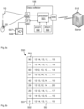
- Fig. 1 schematically illustrates a field 100 of crops comprising multiple plots, such as plot 101 and a crop scanner 102.
- the crops or plants in one plot may be referred to as group of individuals or a population and the aim is a genetic gain in that population without genetic testing or assisted by genetic testing.
- the crops may be wheat, rice cereal and other crops such as canola and grapevines.
- Crop scanner 102 comprises a line scan distance sensor 103, a mover system 104, a rotary encoder 105 and a data collector 106. It is noted that some examples herein relate to a vehicle as crop scanner 102. However, in other examples, crop scanner may be a fixed gantry and the crops are moved through the gantry, such as on a conveyor belt.
- Fig. 2 illustrates line scan distance sensor 103 mounted on the crop scanner 102 (not shown in Fig. 2 ) as seen from the front.
- a possible device may be LMS400, 70 ⁇ FOV, SICK AG, Waldkirch, Germany.
- Line scan distance sensor 103 measures a distance 201 of the crops 202 from the sensor along a line 203.
- Line scan distance sensor 103 illuminates the crops 202 with a laser beam 204 at a measurement angle 205.
- the measurement angle 205 is taken between a vertical line 206 and the laser beam 204.
- the measurement angle 205 defines the line 203 in the sense that as the measurement angle 205 increases, the laser beam 204 is directed at points along the line 203. In other words, if the measurement angle 205 is increased rapidly so that the laser beam 204 rotates around the sensor 103, a person would be able to see a red line on the ground in the case of a red laser.
- Sensor 103 detects reflected light 207 and measures the time of flight, that is, the time between sending the laser beam 204 and receiving the reflected light 207. Sensor 103 can then calculate distance 201 by multiplying the time of flight by the speed of light. In another example, sensor 103 detects a phase shift and calculates the distance based on the phase shift. This way, sensor 103 generates distance data indicative of the distance 201 of the crops from the sensor 103 at the measurement angle 205. Sensor 103 pulses laser beam 204 while increasing angle 205 to generate distance data for multiple points along line 203.
- scanner 103 may comprise a rotating mirror, prism or MEMS device to increase angle 205 and may generate distance data at measurement angle increments of between 0.1 degrees and 1 degree, that is, for an aperture angle of 70 degrees there would be 70 to 700 distance data points along line 203 where the number of data points may be configurable. It is noted that the multiple values for the measurement angle may vary from one scan line to the next. In other words, the points where the crop is scanned may not be aligned across different scan lines. In the proposed solution, this has the advantage that further data becomes available since regions that may have been overstepped in one scan line are scanned in the next scan line.
- the line scan distance sensor generates intensity data indicative of an intensity of the reflected light.
- the intensity is indicative of the reflectance of the illuminated material and changes between fresh green leaves, dry brown leaves and soil. This distinction can be emphasised by using red laser light.
- the data collector 106 in this example processes the intensity data from the distance sensor 103 together with or separately to the distance data as described further below.
- the distance sensor 103 may scan the crops 202 at a constant rate of laser pulses, which means that the distance between data points (spatial sampling rate) is minimal directly under the sensor 103 (in the direction of vertical 206) and maximal at the distal ends of line 203. In other words, the data points are further apart from each other towards the end of scan line 203 than in the middle of it.
- crop scanner 102 comprises mover system 104.
- Mover system 104 moves the line scan distance sensor 103 substantially perpendicular to the distance 201 of the crops from the sensor. In Fig. 2 , the movement would be into the plane of the drawing keeping a constant distance 210 from the ground as defined by the geometry of the mover system 104.
- mover system 104 comprises three wheels, where two wheels are arranged in parallel to line 203 and the third wheel is arranged behind and in line with the left wheel of the two front wheels.
- the mover system 104 may be moved by an operator, such as by pushing the mover system 104.
- mover system 104 comprises one or more motors and autonomous navigation system based on GPS and/or inertial navigation systems.
- Crop scanner 102 further comprises rotary encoder 105.
- the rotary encoder 105 may be associated with the mover system such as by being mounted onto one of the wheels.
- Rotary encoder 105 generates movement data indicative of a movement of the distance sensor substantially perpendicular to the distance 201 of the crops from the sensor as defined by the mover system 104.
- Fig. 3 illustrates an example rotary encoder 105 mounted on a shaft 301, which may be the axle of the wheel.
- Rotary encoder 105 comprises a quadrature encoder 302 connected to shaft 301, a light source 303, such as an LED, a lens 304 and a photo detector 305.
- Quadrature encoder 302 comprises alternating transparent sections (shown in white) and occluding sections (shown in black).
- An outer ring 306 comprises 40 sections, while an inner ring 307 comprises 80 sections.
- Light from the LED 303 is focussed by lens 304 and passes through the quadrature encoder 302.
- the quadrature encoder 302 rotates together with shaft 301 the light is alternatingly blocked or transmitted, which results in a square waveform at the output of the photo detector 305.
- the frequency of the square waveform is directly related to the rotation speed of the shaft 301.
- the photo detector 305 outputs two square waveforms where one square waveform has twice the frequency of the other square waveform.
- Data collector 106 in Fig. 1 is connected to photo detector 305 and receives the square waveforms. By detecting the relationship between the two square waveforms processor data collector 106 can determine the direction of rotation as well as the speed of rotation.
- the data collector 106 determines that the crop scanner 102 has moved by a predefined distance.
- the circumference of the wheels of the crop scanner 102 is 0.8 m and as a result, each rotation of the shaft relates to a moved distance of 0.8 m.
- the inner ring 307 comprises 80 transitions between transparent and occluding sectors, each edge of the square waveform associated with the inner ring 307 corresponds to a movement of 0.01 m, that is, the rotary encoder 105 provides a quadrature pulse every 0.01 m travel. For 1.5 m/s, this would result in 150 pulses per second.
- the rotary encoder 105 may be a DFV60A-22PC65536 (SICK AG, Waldkirch, Germany) providing 65,536 pulses per revolution which leads to a pulse every 12 ⁇ m (at a wheel circumference of 0.8 m).
- the rotary encoder may be mounted on the driving wheel of a conveyor belt or similar mover.
- the line scan distance sensor 103 is downwardly directed to the ground, which is suitable for vertically growing crops such as grain including wheat and rice. In other examples, the line scan distance sensor is directed sidewardly, which is suitable for fruit crops including grape vines.
- Fig. 4 is a plan view of plot 101 in Fig. 1 .
- scan lines 402 comprising scan line 203 as shown in Fig. 2 .
- scanner 102 scans plot 101 along further scanlines, such as further scanline 403.
- the scanning rate is 100 Hz, which means that scanner 103 creates 100 scan lines per second. At a speed of 1.5 m/s this would result in 0.015 m between scan lines.
- pulses 404 from the rotary encoder 105. As can be seen in Fig.
- the indications of pulses 403 are significantly more frequent than the indication of scan lines 402, which improves the overall accuracy of the system and in particular, the location reference of the scan lines 402.
- the accuracy of that position is limited by the distance between pulses 404. That is, if the distance between pulses is 0.001 m, then the accuracy of the location of the scan lines 402 is also 0.001 m in the example where the data collector 106 counts the number of pulses 404 between scan lines 402.
- the aim is to calculate an absolute quantitative measure, such as biomass, it is important that the location of the scan lines is accurate.
- Fig. 4 also shows a leaf 410, which is part of the biomass of plot 101.
- Leaf 401 is scanned by three scanlines 203, 403 and 411 and the accurate distance between the scan lines 203/403 and 403/411 is indicated by the number of pulses 404 from rotary encoder 105. Due to the accurate distance measure, the size of the leaf and therefore the absolute measure of biomass can be accurately calculated.
- the absolute measure of biomass may be biomass per square meter or per another fixed surface area.
- the following table provides further example configurations of the encoder rate and scan rate: speed [m/s] # sectors pulses [1/s] enc. resolution [mm] scan rate [1/s] line dist [mm] 1 800 1000 1 100 10 1.5 800 1500 1 100 15 3 800 3000 1 100 30 5 800 5000 1 100 50 10 800 10000 1 100 100 1 1600 2000 0.5 200 5 1.5 1600 3000 0.5 200 7.5 3 1600 6000 0.5 200 15 5 1600 10000 0.5 200 25 10 1600 20000 0.5 200 50 1 1600 2000 0.5 500 2 1.5 1600 3000 0.5 500 3 3 1600 6000 0.5 500 6 5 1600 10000 0.5 500 10 10 1600 20000 0.5 500 20
- the line distance is greater than the encoder resolution, which means that multiple encoder pulses are received between scan lines, which enables accurate relative local positioning of the scan lines.
- the encoder rate is at least ten times higher than the scanning rate. It is further shown that a large speed of 10 m/s can be used, which enables scanning of large plots in acceptable time or scanning of a larger number of plots to select from a larger number of individuals or groups of individuals, such as plots. This leads to higher genetic gain, that is higher performing crops, than with existing methods over the same time period.
- Fig. 5a illustrates data collector 106 in more detail.
- data collector 106 comprises processor 501 connected to program memory 502, data memory 503, data input port 504 and user interface port 505.
- the program memory 502 is a non-transitory computer readable medium, such as a hard drive, a solid state disk or CD-ROM.
- Software, that is, an executable program stored on program memory 502 causes the processor 501 to perform the method in Fig. 6 , that is, processor 501 controls scanner 103 to measure a distance and generate distance data, controls the mover system 102 to move the scanner and generate movement data, associates the distance data with positioning data and stores the result on data memory 503.
- Processor 501 may also send the determined positioning data associated with the distance data via communication port 506 to a server 510, which may then calculate a quantitative trait of the plant on the current plot 101. This allows more complex calculations that would be difficult to perform on the data collector 106 due to hardware limitations of mobile computing systems.
- the processor 501 may receive data, such as distance data, from data memory 503 as well as from input port 504 and the user port 505, which is connected to a display 507 that shows a visual representation 508 of the plot 101 to a user.
- the processor 501 receives distance data from rotary encoder via input port 504, such as by using a Wi-Fi network according to IEEE 802.11 or a CAN bus.
- the processor 501 receives and processes the distance data in real time. This means that the processor 501 associates and stores the distance data every time distance data of a line scan is received from rotary encoder 105 and completes this calculation before the rotary encoder 105 sends the next line scan update.
- data collector 106 is implemented as a microcontroller, such as an Atmel ATmega328.
- Data collector 106 may comprise a counter that is incremented each time a pulse from rotary encoder 105 is detected on a pin of the microcontroller.
- the microcontroller reads the value of the counter, stores the value of the counter associated with the data from the scanner 103 and resets the counter to zero.
- data collector 106 is implemented as a tablet computer that collects the data and may readily upload the data to server 510 using a cellular or Wifi network.
- Fig. 5b illustrates an example data format. It is noted that the sensor 103 repeatedly measures the distance of the crops 202 from the sensor 103 along multiple lines to generate distance data for each of the multiple lines.
- the data collector 106 associates the distance data from each of the multiple lines with relative positioning data indicative of a relative position of that line.
- data collector 106 stores the distance values as rows, such as first row 551.
- First row 551 has a first data field 552 for the relative positioning data and a second data field 553 for the distance data points from sensor 103.
- the first data fields 552 holds the number of pulses from rotary encoder 105 from the start of the plot 101.
- first data field may hold the distance in metres or millimetres from the start of the plot.
- Fig. 6 illustrates a method 600 as performed by processor 501 for scanning crops.
- Processor 501 generates control signals to control the distance sensor 103 to illuminate 601 the crops with laser light at a measurement angle that defines a line.
- Processor 501 measures a distance of the crops from the distance sensor 103 at one or more points along the line by detecting reflected light and measuring the time of flight between illuminating the crops at step 601 and receiving the reflected light in step 602.
- Processor 501 uses the measurement to generate 603 distance data indicative of the distance of the crops from the sensor at the measurement angle.
- the distance data is generated by the distance sensor 103.
- Processor 501 then generates control signals to move 604 the distance sensor substantially perpendicular to the distance of the crops from the distance sensor.
- an operator may move the distance sensor.
- Processor 501 may generate a user interface to guide the operator, such as by creating a graphical representation of the current speed in relation to the optimal speed.
- Processor 501 may also indicate the relative location within the plot 101 or a GPS location within the field 100.
- Rotary encoder 105 generates 605 movement data indicative of a movement of the distance sensor 103 substantially perpendicular to the distance of the crops from the sensor.
- Processor 501 associates 606 the distance data from the distance sensor with relative positioning data based on the movement data.
- the relative positioning data may be the number of pulses as described above or may be derived value, such as a relative distance.
- Processor 501 finally stores 607 the distance data associated with the relative positioning data on a data store.
- processor 501 stores the distance data associated with the relative positioning data on an SD card that can be removed and inserted into a computer to read-out and process the data.
- processor 501 stores the distance data associated with the relative positioning data on a cloud storage, which causes server 510 to process the distance data to calculate a crop trait value, namely an absolute measure of biomass.
- Uploading the distance data may comprise uploading more than 5,000 distance data points to the processing server 510 to cause the processing server 510 to calculate one crop trait value based on the more than 5,000 distance data points.
- This may relate to a plot size of 7000 mm, such that all data points of one plot are uploaded to calculate a single crop trait value.
- the uploading of the large number of distance data points means that only a small amount of processing power is required in the data collector 106 and the bulk of the processing for aggregating the data points can be performed on the server 510.
- server 510 calculates from the large number of distance data points a single crop trait value for each plot 101.
- server 510 may be hosted on desktops, laptops or mobile devices.
- server 510 is implemented in a distributed (cloud) computing environment, such as Amazon AWS.
- a supervisor may determine a number of virtual machines and instantiate those virtual machines on the cloud to process the distance data points as described herein. Once the distance data points are processed, the supervisor destroys the virtual machines. This allows for highly computationally expensive calculations to be performed relatively quickly without the need for investing into expensive hardware. Since the distance data from each plot can be processed separately, the specific processing task can be parallelised on multiple virtual machines effectively. In one example, the supervisor instantiates one virtual machine for each plot.
- Fig. 7a illustrates a single crop 700 growing on ground 701 and having leaves 702 and seeds 703.
- Solid dots indicate the locations where the laser light 204 hits the crop or the ground. That is, each dot represents one distance data point.
- Server 510 can calculate for each distance data point a height measurement.
- Server 510 then calculates a histogram by counting the number of height measurements in each of multiple bins.
- Fig. 7b illustrates a histogram 750 of the height of the dots in Fig. 7a .
- Histogram 750 includes a first peak 751 for height measurements around zero indicating reflections off the ground 701.
- Histogram 750 further includes a second peak 752 indicating reflections off the leaves 702 of crop 700 and a third peak 753 indicating reflections off the seeds 703. While the histogram 750 for a single crop may be irregular, server 510 creates a similar histogram for all data points of the plot 101.
- Fig. 8 illustrates a histogram for the entire plot 101. Compared to Fig. 7b , the histogram in Fig. 8 is more regular.
- Server 510 can now extract features from the histogram. For example, server 510 may identify a first peak or maximum 801 and use a height value 802 of the first peak 801 as a feature.
- Server 510 may further receive historical crop trait values of sampled crops. For example, workers can cut samples from multiple plots and manually measure the biomass in these sample.
- Server 510 calculates the feature for each of the multiple plots and correlates the feature to the sampled biomass measurement.
- server 510 may use a linear regression model to calculate a linear relationship between the feature, that is the height of the first peak 801, and the biomass based on the historical sample data. Server 510 can then apply this correlation, that is the linear relationship, to plot 101. This allows the server 510 to calculate an estimated biomass as a crop trait value without the need for manually and destructively sampling the plot 101.
- the parameters for the relationship between sampled biomass and histogram features are specific to each crop. That is, wheat would have a different relationship than rice, for example.
- Server 510 may automatically detect the edges of each plot by detecting that the majority of data points have a ground value of about zero height. In one example, it is assumed that the scan line 203 spans a single plot, such that for each line all points belong to the same plot. Server 510 can then iterate over all scan lines and calculate the histogram of the current scan line. If the histogram has more peaks than the ground peak 751 then the scan line is added to the data for that plot. If the histogram has only the ground peak 751, server 510 concludes that the end of the current plot has been reached and a new plot can be started for the next scan line that shows more peaks than the ground peak 751.
- server 510 can select out of multiple plots those with the highest estimated biomass, which means the plot is a highly performing plot.
- server 510 may generate a user interface that shows the estimated biomass for each plot such that an operator can see which plot should be selected for further breeding.
- Server 510 may also generate and display a ranking of plots such that the operator can select the plot at the top of the ranking for further breeding.
- Each plot may be associated with a plot identifier, population or genotype and the server 510 may automatically select the plot identifier, population or genotype with the highest estimated biomass for further breeding. That is, server 510 creates a display or a digital document comprising an indication of the selected plot identifier or genotype.
- Map 900 comprises a rectangle for each plot and the fill of each rectangle, such as colour, shading or pattern, indicates the estimated biomass or other crop trait value. For example, darker rectangles indicate plots with a higher crop trait value while lighter rectangles indicate plots with a lower crop trait value.
- the crops in all plots are of the same variety and the variation in crop trait values is caused by a variation in environmental conditions, such as water supply.
- the frequent scanning of the crops which is enabled by this disclosure, allows the monitoring of the influence of those conditions by monitoring the crop trait value directly. Irrigation, for example, can then be automatically actuated for those plots with a lower crop trait value.
- Fig. 10 illustrates an image 1000 that server 510 may create.
- server 510 adds a dot for each of the data points of the current plot into the image considering only the height and the location along the scan line 203 but disregarding the location of the data points along the direction of movement 401 (shown in Fig. 4 ).
- the image 1000 clearly shows the structure of the crop and can be considered as an accumulated cross-section through the plot. This gives the operator additional insight which makes the selection of plots or genotypes or other resulting actions more accurate.
- the dots may also be colour coded to indicated the intensity. Since fresh leaves, dry leaves and soil have different reflectance and therefore lead to different intensities of reflected light, the colour code can graphically distinguish between these materials.
- biomass production While some examples above relate to biomass production, other traits may be possible that were difficult to ascertain with existing methods. For example, biomass production during increased irrigation or other change in environment. Other time dependent traits may also be considered including change of canopy height over two weeks, for example. In further examples, traits may include Water use efficiency, Nutrient use efficiency (particularly nitrogen and phosphorus), Weed competitiveness, Tolerance of mechanical weed control, Pest/disease resistance, Early maturity (as a mechanism for avoidance of particular stresses) and Abiotic stress tolerance (i.e. drought, salinity, etc).
- the artificial selection method of the present invention is useful for selecting an individual or a population of individuals or reproductive or regenerative material from the individuals for use in breeding or transgenic approach. Accordingly, the present invention also provides a process for improving the rate of genetic gain in a population comprising performing the method of the present invention according to any embodiment described herein and selecting an individual or population of individuals, such as a plot, based on one or more phenotypes, that is, a desirable estimated crop trait value.
- a low crop trait value means a crop trait value sufficient to improve a genetic gain in the population if the selected individual or population of individuals is mated to another individual or group of individuals e.g., an individual or population of individuals that also has a desirable estimated crop trait value as determined against the same or different parameter(s). It is noted that a low crop trait value may be desirable, such as water use.
- the process comprises obtaining reproductive or regenerative material from the selected individual.
- the term "obtaining reproductive or regenerative material” shall be taken to include collecting and/or storing and/or maintaining germplasm such as the selected individual pollen from the selected individual, seed etc. produced using the germplasm of the selected individual, such as for use in conventional breeding programs; and collecting and/or storing and/or maintaining cells such as embryonic stem cells, pluripotent or multipotent stem cells, fibroblasts, or organelles such as nuclei, mitochondria or chloroplasts from the selected individual, optionally transformed to include one or more genes or nucleic acids for conferring a desired attribute on an organism, for the production of transformed organisms carrying the genetic material of the selected individual.
- the present invention clearly extends to any reproductive or regenerative material obtained by performing the process of the present invention and an organism produced therefrom.
- This organism may produce a genetic gain in the population that is substantially the same as the expected genetic gain or actual genetic gain from the entire germplasm of the selected individual.
- expected genetic gain is a theoretical value
- actual genetic gain is a value determined from test matings in a population.
- the reproductive or regenerative material is generally stored for a prolonged period for subsequent use and it is desirable in such circumstances to maintain records of the material. Accordingly, the present invention also provides a computer-readable medium for use in artificial selection said computer-readable medium comprising a database of reproductive or regenerative material obtained by performing a process of the invention according to any embodiment described herein.
- Crop scanner 103 may be an adaptable mobile platform for the deployment and testing of proximal imaging sensors in vineyards.
- a SICK LMS-400 light radar (LiDAR) mounted on scanner 103 is capable of producing precise ( ⁇ 3mm) 3D point clouds of vine rows. Scans of multiple grapevine varieties and management systems have demonstrated that scanner 103 can be useful in a variety of vineyards.
- the frame may include more instruments.
- computational processes can be improved and automated as more correlations between growth features and LiDAR scans are developed.
- This disclosure provides an adaptable proximal sensing scanner 103and demonstrates how it is able to use light radar (LiDAR) to capture point clouds of vine size and structure at a number of different growth stages with differing canopy management systems. Beyond producing 3D scans there is provided a computational method that uses LiDAR scans to estimate pruning weight, an indicator of vegetative vine vigour which requires considerable labour costs to measure.
- LiDAR light radar
- the frame for scanner 103 is made of lightweight structural-aluminium and weighs -200 kg. It is 3 m long, and has a wheelbase that can be adjusted between 1.2 and 3 m to enable operation in a variety of row spacings with maximum stability.
- the mast can be raised for measuring taller canopies and lowered for transportation. When raised, the mast is 3.2 m tall and stabilized by an additional aluminium support beam that is stored on the frame.
- Scanner 103 measures 2.1 m tall when the mast is lowered.
- Scanner 103's principle sensor, the LMS-400 LiDAR ( Figure 1a) can be mounted in virtually any position on the frame.
- the LiDAR can be rotated to scan anywhere from zero degrees, pointing straight at the ground, 90 degrees, pointed straight at the canopy, or 180 degrees, positioned underneath the canopy, aimed skyward. For all the scans presented here the LiDAR was mounted 2.25 m above the ground, on the centre mast and angled 45 degrees.
- the frame is equipped with three wheels: the front two wheels have built-in electric motors and there was one free-pivoting wheel in the rear.
- the rear tire is 21 inches in diameter and allows scanner 103 to have a zero degree turn radius, which was important for two reasons: First, looping between vineyard rows may be difficult if the platform was less manoeuvrable. Second, since the front two wheels are powered independently, scanner 103 can be programmed to operate autonomously.
- the two wheels in the front are 16 inch MagicPie 4 eBike-motors (Golden Motor Technology Co. Ltd., Changzhou, China). Each wheel is powered independently by a 48v lithium ion battery (Golden Motor Technology Co. Ltd., Changzhou, China).
- the wheels are operated and driving speed is controlled by two thumb-throttle controllers mounted on scanner 103's rear handle bars.
- Scanner 103 is also equipped with a 24v lithium ion battery (Golden Motor Technology Co. Ltd., Changzhou, China) which is used to power the instruments.
- the power from the battery is converted into four separate outputs: a 5v output, two 12v outputs and a 24v output (Helios Power Solutions Pty. Ltd., Sydney, Australia).
- a variety of voltages is created to power and test different sensors.
- the LiDAR mounted to scanner 103 is a SICK model LMS-400-2000 ( Figure 1a; SICK AG, Waldkirch, Germany).
- the laser is an eye-safe red laser (650 nm) and scans a 70 degree field of view.
- the LMS-400 has a range of 0.7 m to 3 m and can be programmed to scan between speeds of 250 to 500 Hz.
- the LiDAR produces polar coordinates (distance and angle) from the resolved time of flight from the laser, which are then converted to xyz coordinates to generate a point cloud. Additionally, the LiDAR produces information about the reflectance of the scanned surface.
- the reflectance value is related to the ability of a material to reflect the LiDAR signal back to the sensor: the higher the reflectance value, the more reflective the surface.
- the linear distance travelled by -scanner 103 is measured with a wheel encoder which provides sub-millimetre distance resolution. Viewed from the handlebars, the wheel encoder is in contact with the front left tire. (DFV60A-22PC65536, SICK AG, Waldkirch, Germany).
- the LiDAR and encoder data are integrated via a junction box (SICK CMD490-0103; SICK AG, Waldkirch, Germany).
- a Spatial GPS/IMU (Advanced Navigation, Sydney Australia) unit is attached with double-sided tape to the top of the LiDAR. The Spatial unit is used to record data about the angle of the LiDAR and scanner 103's spatial position ( ⁇ 2 m).
- the LiDAR, GPS and encoder data are captured using the field laptop running bespoke java software, which provides a user interface presenting a map of the GPS, input dialogs for the experiment name and run number.
- the LiDAR data is stored in a custom binary format (.PLF), while the GPS and encoder are combined and stored as text comma separated values (CSV) file format (.GPS).
- .PLF custom binary format
- CSV text comma separated values
- a custom-made piece of java software converts the .PLF and GPS data to a standard point cloud format such as the Stanford triangle format (.PLY).
- the integrated point cloud and encoder data, saved as a .PLY file, are visualized using the open-source software CloudCompare.
- Point clouds are processed and cleaned using two applications. First the points are filtered by their reflective intensity, or reflectance values, using an intensity selection plugin built into CloudCompare. All points with reflective intensities less than or equal to 1 are removed. Second, PCL wrapper plugin is used, which employs a nearest neighbour filtering algorithm. In detail, 10 points are used for mean point distance estimation and the standard deviation multiplier threshold is 1.00.
- Scanner 103 is capable of being wheeled onto a trailer by one person, anchored and ready for transport in ⁇ 30 minutes.
- the ease of transport gives the platform an advantage over some previous phenotyping platforms which are more cumbersome and difficult to transport.
- Scanner 103 is driven at an average speed of 1 m/s . Given that both sides of the vine had to be scanned, a one km vineyard-row is able to be scanned every hour.
- the first step in the workflow is choosing an area to scan. Because of the adjustable wheel base, scanner 103 could be used in almost any commercial vineyard. Vines in an test were of the variety Shiraz grown at a research vineyard in Sydney, South Australia. The smallest units identified for scans were single, ⁇ 3.6 m panels (3 vines per panel, with spacing between vines of 1.8 m) and the largest area scanned, to date, was a 500 m row containing 93 similar sized panels (data not shown). The 500 m row produced ⁇ 1 GB .PLY files for visualization.
- the point cloud was cleared of erroneous data points.
- the LMS-400 gives precise spatial and reflectance data at a high rate, it is designed to operate below 2000 lux and not under high light conditions.
- Lux values in indirect sunlight commonly range between 1 thousand lux on an overcast day to 130 thousand in direct sunlight.
- High light levels are the cause of spurious, low-intensity blue points seen between the LiDAR and the vines.
- the erroneous measurements are all low reflectance values and can be removed by filtering the scan based on a set reflectance value.
- Points with reflectance values ⁇ 1.0 were removed from the scan using the ⁇ filter points by value' plugin in CloudCompare. There are 1.49 million total points, and 28 % of those points were ⁇ 1.0.
- the reflectance threshold was chosen qualitatively and removed spurious points without significantly affecting the biological interpretation of the scan. Green leaf material had a reflectance value between one and five.
- the nearest neighbor statistical outlier plugin in CloudCompare removed sparse outliers based off the distance of an individual point from its neighbors. By applying these filters, point-clouds were reduced to only the scanned objects. There may be 1.12 million points. After the filter removing statistical outliers is applied there are 1.04 million points in the final point cloud on which any computational analysis would be performed.
- LiDAR is able to capture vine size and structure at all growth stages
- scanner 103 was used to scan a diversity of vine growth throughout 2015 growing season. Vines differ remarkably in size, age, management style and variety, which ultimately affects fruit quality and productivity. Thus, it was important to test the practical limitations of LiDAR on a variety of vines and growth-stages.
- the LiDAR may be able to distinguish leaves from bunches and estimate yield.
- This disclosure provides scanner 103 as a proximal sensing platform for use in Australian vineyards. Its frame will provide a flexible platform for testing multiple sensors in a variety of regions, management styles and grape varieties.
- the principal sensor on the frame is a LiDAR scanner.
- the 2D line scanner can scan one side of the vine canopy at a time and produce high definition 3D point clouds of vine growth.
- the ability of the LiDAR to capture growth features has not been limited to any specific variety of vine or management style It may be possible to achieve ground-truthing LiDAR scans and include data from any additional instruments - with conventional measurements of vine growth.
- other types of sensors such as stereo-RGB cameras and hyperspectral scanners.
Description
- The present application claims priority from
Australian provisional application 2016905220 filed on 16 December 2016 Australian provisional application 2017903379 filed on 22 August 2017 - This disclosure is related to systems and methods for scanning crops. In particular, but not limited to, this disclosure relates to scanning crops to determine crop trait values (i.e. biophysical parameters), including biomass and growth, for artificial selection.
- Selective breeding comprises the determination of crop traits as phenotypes and selecting those crops with desired traits for further propagation. Crop traits may include biomass and canopy height and the determination of biomass and canopy height may involve destructive testing and/or LIDAR measurements. LIDAR measurements are performed by directing a laser beam at the crop and measuring the return time of the reflection off the crop. Based on the return time a distance to the LIDAR sensor can be determined, which, in turn, can be used to estimate biomass and canopy height.
- Current LIDAR crop scanners use GPS to record multiple locations while scanning the crop. For example, Pittman et al. disclose a modified golf cart fitted with a LIDAR sensor and GPS configured to output spatial data at a rate of 10 Hz (Jeremy Joshua Pittman, Daryl Brian Arnall, Sindy M. Interrante, Corey A. Moffet and Twain J. Butler. "Estimation of Biomass and Canopy Height in Bermudagrass, Alfalfa, and Wheat Using Ultrasonic, Laser, and Spectral Sensors". ).
- Chen discloses systems for LiDAR Remote Sensing of Vegetation Biomass (Chen, Q. Lidar remote sensing of vegetation biomass. In Remote Sensing of Natural Resources; Wang, G., Weng, Q., Eds.; CRC Press, Taylor & Francis Group: Boca Raton, FL, USA, 2013; pp. 399-420.). Chen further discloses that the 3D coordinates of laser returns collected at individual scanning positions are local and relative to the scanners. Further, according to Chen the individual datasets have to be georeferenced to a common coordinate system based on features visible to multiple positions, which is not a trivial task. To make it more difficult, ground-based LiDAR systems can acquire data with point densities 100-1000 times higher than the average point density of airborne small-footprint LiDAR systems. Such massive volumes of data pose a significant challenge in developing fast, automatic, and memory-efficient software for data processing and information extraction.
- Biber et al. disclose an autonomous agricultural robot comprising a 3D MEMS LIDAR providing a full scan at 59x29 pixels across the field of view of 50x60 degrees (Peter Biber, Ulrich Weiss, Michael Doma, Amos Albert. Navigation System of the Autonomous Agricultural Robot "BoniRob". Workshop on Agricultural Robotics: Enabling Safe, Efficient, and Affordable Robots for Food Production (Collocated with IROS 2012), Vilamoura, Portugal). A RANSAC algorithm is used to fit a Hessian plane equation to the data. The detected plane is then refined by a Least Squares fit. Number of inliers and residuals of the Least Squares are then considered to detect failed ground detection. Also, a Kalman filter tracks the state of the plane over time. If the ground detection failed the state is just propagated. Depending on the field the detected ground can correspond to soil or the canopy. Also the thresholds for plane detection have to be set according to the application. Further, as a side effect of ground detection it is possible to derive the height and the tilt angle of the scanner so only the x/y position of the scanner are defined manually in the configuration.
US 2015/0015697 A1 discloses a system for plant parameter detection, including: a plant morphology sensor having a first field of view and configured to record a morphology measurement of a plant portion and an ambient environment adj acent the plant, a plant physiology sensor having a second field of view and configured to record a plant physiology parameter measurement of a plant portion and an ambient environment adjacent the plant; and a computing system configured to: identify a plant set of pixels within the physiology measurement based on the morphology measurement; determine physiology values for each pixel of the plant set of pixels; and extract a growth parameter based on the physiology values.US 2014/0180549 A1 discloses systems for identifying a plant in a field with pixel-level precision and taking an action on the identified plant, also with pixel level precision. - Throughout this specification the word "comprise", or variations such as "comprises" or "comprising", will be understood to imply the inclusion of a stated element, integer or step, or group of elements, integers or steps, but not the exclusion of any other element, integer or step, or group of elements, integers or steps.
- A system for calculating biomass of crops is provided according to claim 1.
- It is an advantage that the use of a line scan distance sensor is more robust and computationally more efficient than the use of a 3D scanner. It is a further advantage that accurate relative positioning data can be created from the rotary encoder data. This allows accurate relative spatial alignment of sequential line scans. As a result, an extremely high resolution in the direction of movement can be achieved. The combination of a line scan distance sensor with a rotary encoder provides an accuracy that is sufficient to resolve individual leaves which allows accurate crop monitoring.
- The mover may be a vehicle. The mover may be a gantry.
- The line scan distance sensor may be downwardly directed towards the ground. The line scan distance sensor may be directed sidewardly.
- The relative positioning data may have an accuracy of 1 cm or higher.
- The rotary encoder may be configured to generate detection signals at an encoder rate that is higher than a scanning rate of line scans from the line scan distance sensor when the mover moves the line scan distance sensor at a scanning speed.
- The scanning speed may be 1 m/s or faster.
- The scanning rate may be 500 Hz or less.
- The encoder rate may be at least ten times higher than the scanning rate.
- The line scan distance sensor may be further configured to generate intensity data indicative of an intensity of the reflected light and the data collector may be configured to associate the intensity data from the distance sensor with relative positioning data based on the movement data from the rotary encoder and to store the intensity data associated with the relative positioning data on the data store.
- The light may be laser light. The laser light may be red laser light having a wavelength between 625 nm and 740 nm.
- The system may further comprise a second line scan distance sensor to measure a distance of the crops from the second line scan distance sensor along the line, wherein the second line scan distance sensor is offset or tilted relative to the first line scan distance sensor.
- The line scan distance sensor may configured to repeatedly measure the distance of the crops from the sensor along multiple lines to generate distance data for each of the multiple lines, and the data collector may be configured to associate the distance data from each of the multiple lines with relative positioning data indicative of a relative position of that line.
- A method for calculating biomass of crops is provided according to claim 8.
- The method may further comprise uploading the distance data associated with the relative positioning data to a processing server to cause the processing server to calculate an absolute measure of biomass.
- Uploading the distance data may comprise uploading more than 5,000 distance data points to the processing server to cause the processing server to calculate the absolute measure of biomass based on the more than 5,000 distance data points.
- Measuring the distance of the crops from the distance sensor may comprise providing a scan angle value associated with a distance value and generating the distance data may comprise calculating a crop height above ground based on the distance value and the scan angle value.
- Calculating the crop height above ground may be based on a predetermined sensor height above ground.
- The distance data may further comprise intensity data.
- The distance data may comprise a scan angle value associated with a distance value.
- Calculating the crop height above ground may be based on a predetermined sensor height above ground.
- The distance data may comprise multiple line scans of multiple monitoring areas.
- Each of the multiple monitoring areas may be associated with a different crop population.
- The method may further comprise automatically detecting the multiple monitoring areas based on the distance data and the relative positioning data.
- The method may further comprise generating a display to indicate a highly performing monitoring area out of the multiple monitoring areas based on the absolute measure of biomass.
- The method may further comprise selecting a population associated with one of the multiple monitoring areas based on the absolute measure of biomass for further breeding.
- An example will be described with reference to
-
Fig. 1 schematically illustrates a field comprising multiple plots and a crop scanner. -
Fig. 2 is an front elevation view of a line scan distance sensor. -
Fig. 3 illustrates an example rotary encoder. -
Fig. 4 is a plan view of one of the plots inFig. 1 . -
Fig. 5a illustrates the data collector fromFig. 1 in more detail. -
Fig. 5b illustrates an example data format. -
Fig. 6 illustrates a method for scanning crops. -
Fig. 7a illustrates a single crop with data points. -
Fig. 7b illustrates a histogram of data points for one crop. -
Fig. 8 illustrates a histogram for the entire plot. -
Fig. 9 illustrates a map of the field created by the server fromFig. 5 . -
Fig. 10 illustrates an image of a plot created by the server fromFig. 5 . - This disclosure provides systems and methods for accurate and high-throughput crop phenotyping. The disclosed systems associate line scanner data with a high resolution rotary encoder to provide distance data with high local alignment accuracy. This allows for a more accurate, faster and non-destructive determination of crop traits, which can be used to select the best performing crops from a larger number of populations, such as plots, for future breeding.
-
Fig. 1 schematically illustrates afield 100 of crops comprising multiple plots, such asplot 101 and acrop scanner 102. The crops or plants in one plot may be referred to as group of individuals or a population and the aim is a genetic gain in that population without genetic testing or assisted by genetic testing. The crops may be wheat, rice cereal and other crops such as canola and grapevines.Crop scanner 102 comprises a linescan distance sensor 103, a mover system 104, arotary encoder 105 and adata collector 106. It is noted that some examples herein relate to a vehicle ascrop scanner 102. However, in other examples, crop scanner may be a fixed gantry and the crops are moved through the gantry, such as on a conveyor belt. -
Fig. 2 illustrates linescan distance sensor 103 mounted on the crop scanner 102 (not shown inFig. 2 ) as seen from the front. A possible device may be LMS400, 70∘ FOV, SICK AG, Waldkirch, Germany. Linescan distance sensor 103 measures adistance 201 of thecrops 202 from the sensor along aline 203. Linescan distance sensor 103 illuminates thecrops 202 with alaser beam 204 at ameasurement angle 205. In this example, themeasurement angle 205 is taken between avertical line 206 and thelaser beam 204. Themeasurement angle 205 defines theline 203 in the sense that as themeasurement angle 205 increases, thelaser beam 204 is directed at points along theline 203. In other words, if themeasurement angle 205 is increased rapidly so that thelaser beam 204 rotates around thesensor 103, a person would be able to see a red line on the ground in the case of a red laser. -
Sensor 103 detects reflected light 207 and measures the time of flight, that is, the time between sending thelaser beam 204 and receiving the reflectedlight 207.Sensor 103 can then calculatedistance 201 by multiplying the time of flight by the speed of light. In another example,sensor 103 detects a phase shift and calculates the distance based on the phase shift. This way,sensor 103 generates distance data indicative of thedistance 201 of the crops from thesensor 103 at themeasurement angle 205.Sensor 103pulses laser beam 204 while increasingangle 205 to generate distance data for multiple points alongline 203. For example,scanner 103 may comprise a rotating mirror, prism or MEMS device to increaseangle 205 and may generate distance data at measurement angle increments of between 0.1 degrees and 1 degree, that is, for an aperture angle of 70 degrees there would be 70 to 700 distance data points alongline 203 where the number of data points may be configurable. It is noted that the multiple values for the measurement angle may vary from one scan line to the next. In other words, the points where the crop is scanned may not be aligned across different scan lines. In the proposed solution, this has the advantage that further data becomes available since regions that may have been overstepped in one scan line are scanned in the next scan line. - In one example,
data collector 106 calculates aheight 208 of thecrop 202 based on the distance data. To that end,data collector 106 calculates avertical distance 209 by:
vertical distance 209 from a mountingheight 210 ofsensor 103 to calculate theheight 208 of thecrop 202. Throughout the following description, when reference is made to calculations based on distance data, this may refer to calculations using the distance data explicitly or calculations using thecrop height 208 that is based on the distance data. - In one example, the line scan distance sensor generates intensity data indicative of an intensity of the reflected light. The intensity is indicative of the reflectance of the illuminated material and changes between fresh green leaves, dry brown leaves and soil. This distinction can be emphasised by using red laser light. The
data collector 106 in this example processes the intensity data from thedistance sensor 103 together with or separately to the distance data as described further below. - It is noted that the
distance sensor 103 may scan thecrops 202 at a constant rate of laser pulses, which means that the distance between data points (spatial sampling rate) is minimal directly under the sensor 103 (in the direction of vertical 206) and maximal at the distal ends ofline 203. In other words, the data points are further apart from each other towards the end ofscan line 203 than in the middle of it. To improve the resolution of the distance data, a second distance sensor may be employed that is offset fromdistance sensor 103 parallel to scanline 203. In both cases, single or multiple sensors, the distance data may be stored in association with a distance alongscan line 203 instead of ascan angle 205 according to line_dist=distance_201 * sin(measurement_angle_205). - As mentioned above,
crop scanner 102 comprises mover system 104. Mover system 104 moves the linescan distance sensor 103 substantially perpendicular to thedistance 201 of the crops from the sensor. InFig. 2 , the movement would be into the plane of the drawing keeping aconstant distance 210 from the ground as defined by the geometry of the mover system 104. In one example, mover system 104 comprises three wheels, where two wheels are arranged in parallel toline 203 and the third wheel is arranged behind and in line with the left wheel of the two front wheels. The mover system 104 may be moved by an operator, such as by pushing the mover system 104. In other examples, mover system 104 comprises one or more motors and autonomous navigation system based on GPS and/or inertial navigation systems. -
Crop scanner 102 further comprisesrotary encoder 105. Therotary encoder 105 may be associated with the mover system such as by being mounted onto one of the wheels.Rotary encoder 105 generates movement data indicative of a movement of the distance sensor substantially perpendicular to thedistance 201 of the crops from the sensor as defined by the mover system 104. -
Fig. 3 illustrates anexample rotary encoder 105 mounted on ashaft 301, which may be the axle of the wheel.Rotary encoder 105 comprises aquadrature encoder 302 connected toshaft 301, alight source 303, such as an LED, alens 304 and aphoto detector 305.Quadrature encoder 302 comprises alternating transparent sections (shown in white) and occluding sections (shown in black). Anouter ring 306 comprises 40 sections, while aninner ring 307 comprises 80 sections. Light from theLED 303 is focussed bylens 304 and passes through thequadrature encoder 302. As thequadrature encoder 302 rotates together withshaft 301 the light is alternatingly blocked or transmitted, which results in a square waveform at the output of thephoto detector 305. The frequency of the square waveform is directly related to the rotation speed of theshaft 301. - As the quadrature encoder has two
rings photo detector 305 outputs two square waveforms where one square waveform has twice the frequency of the other square waveform.Data collector 106 inFig. 1 is connected tophoto detector 305 and receives the square waveforms. By detecting the relationship between the two square waveformsprocessor data collector 106 can determine the direction of rotation as well as the speed of rotation. - More particularly, at each rising or falling edge of the square waveform the
data collector 106 determines that thecrop scanner 102 has moved by a predefined distance. For example, the circumference of the wheels of thecrop scanner 102 is 0.8 m and as a result, each rotation of the shaft relates to a moved distance of 0.8 m. Since theinner ring 307 comprises 80 transitions between transparent and occluding sectors, each edge of the square waveform associated with theinner ring 307 corresponds to a movement of 0.01 m, that is, therotary encoder 105 provides a quadrature pulse every 0.01 m travel. For 1.5 m/s, this would result in 150 pulses per second. While the above examples were used for illustrative purposes, it is noted that significantly higher resolutions may be used, such as 800 sections leading to 1500 pulses per second or one pulse every 0.001 m travel. It is noted that since the encoder is used at the given resolution, a change in speed can be readily considered by the downstream data processing. - The
rotary encoder 105 may be a DFV60A-22PC65536 (SICK AG, Waldkirch, Germany) providing 65,536 pulses per revolution which leads to a pulse every 12 µm (at a wheel circumference of 0.8 m). - In the example of a fixed gantry, the rotary encoder may be mounted on the driving wheel of a conveyor belt or similar mover. In the example of
Fig. 1 , the linescan distance sensor 103 is downwardly directed to the ground, which is suitable for vertically growing crops such as grain including wheat and rice. In other examples, the line scan distance sensor is directed sidewardly, which is suitable for fruit crops including grape vines. -
Fig. 4 is a plan view ofplot 101 inFig. 1 . On the left hand side there is an indication ofscan lines 402 comprisingscan line 203 as shown inFig. 2 . As thescanner 102 moves forwards as indicated byarrow 401scanner 102scans plot 101 along further scanlines, such asfurther scanline 403. In one example, the scanning rate is 100 Hz, which means thatscanner 103 creates 100 scan lines per second. At a speed of 1.5 m/s this would result in 0.015 m between scan lines. On the right hand side are indications ofpulses 404 from therotary encoder 105. As can be seen inFig. 5 , the indications ofpulses 403 are significantly more frequent than the indication ofscan lines 402, which improves the overall accuracy of the system and in particular, the location reference of the scan lines 402. In other words, when thescan lines 402 are assigned to an absolute or relative position withinplot 101 for later calculations, the accuracy of that position is limited by the distance betweenpulses 404. That is, if the distance between pulses is 0.001 m, then the accuracy of the location of thescan lines 402 is also 0.001 m in the example where thedata collector 106 counts the number ofpulses 404 betweenscan lines 402. Especially in application where the aim is to calculate an absolute quantitative measure, such as biomass, it is important that the location of the scan lines is accurate. - As an illustrative example,
Fig. 4 also shows aleaf 410, which is part of the biomass ofplot 101.Leaf 401 is scanned by threescanlines scan lines 203/403 and 403/411 is indicated by the number ofpulses 404 fromrotary encoder 105. Due to the accurate distance measure, the size of the leaf and therefore the absolute measure of biomass can be accurately calculated. The absolute measure of biomass may be biomass per square meter or per another fixed surface area. - The following table provides further example configurations of the encoder rate and scan rate:
speed [m/s] # sectors pulses [1/s] enc. resolution [mm] scan rate [1/s] line dist [mm] 1 800 1000 1 100 10 1.5 800 1500 1 100 15 3 800 3000 1 100 30 5 800 5000 1 100 50 10 800 10000 1 100 100 1 1600 2000 0.5 200 5 1.5 1600 3000 0.5 200 7.5 3 1600 6000 0.5 200 15 5 1600 10000 0.5 200 25 10 1600 20000 0.5 200 50 1 1600 2000 0.5 500 2 1.5 1600 3000 0.5 500 3 3 1600 6000 0.5 500 6 5 1600 10000 0.5 500 10 10 1600 20000 0.5 500 20 - In the above table it can be seen that the line distance is greater than the encoder resolution, which means that multiple encoder pulses are received between scan lines, which enables accurate relative local positioning of the scan lines. In some examples, the encoder rate is at least ten times higher than the scanning rate. It is further shown that a large speed of 10 m/s can be used, which enables scanning of large plots in acceptable time or scanning of a larger number of plots to select from a larger number of individuals or groups of individuals, such as plots. This leads to higher genetic gain, that is higher performing crops, than with existing methods over the same time period.
-
Fig. 5a illustratesdata collector 106 in more detail. In particular,data collector 106 comprisesprocessor 501 connected toprogram memory 502,data memory 503,data input port 504 anduser interface port 505. Theprogram memory 502 is a non-transitory computer readable medium, such as a hard drive, a solid state disk or CD-ROM. Software, that is, an executable program stored onprogram memory 502 causes theprocessor 501 to perform the method inFig. 6 , that is,processor 501controls scanner 103 to measure a distance and generate distance data, controls themover system 102 to move the scanner and generate movement data, associates the distance data with positioning data and stores the result ondata memory 503.Processor 501 may also send the determined positioning data associated with the distance data viacommunication port 506 to aserver 510, which may then calculate a quantitative trait of the plant on thecurrent plot 101. This allows more complex calculations that would be difficult to perform on thedata collector 106 due to hardware limitations of mobile computing systems. - The
processor 501 may receive data, such as distance data, fromdata memory 503 as well as frominput port 504 and theuser port 505, which is connected to adisplay 507 that shows avisual representation 508 of theplot 101 to a user. In one example, theprocessor 501 receives distance data from rotary encoder viainput port 504, such as by using a Wi-Fi network according to IEEE 802.11 or a CAN bus. In one example, theprocessor 501 receives and processes the distance data in real time. This means that theprocessor 501 associates and stores the distance data every time distance data of a line scan is received fromrotary encoder 105 and completes this calculation before therotary encoder 105 sends the next line scan update. - In one example,
data collector 106 is implemented as a microcontroller, such as an Atmel ATmega328.Data collector 106 may comprise a counter that is incremented each time a pulse fromrotary encoder 105 is detected on a pin of the microcontroller. When a line scan signal is received from thescanner 103, the microcontroller reads the value of the counter, stores the value of the counter associated with the data from thescanner 103 and resets the counter to zero. - In other examples,
data collector 106 is implemented as a tablet computer that collects the data and may readily upload the data toserver 510 using a cellular or Wifi network. -
Fig. 5b illustrates an example data format. It is noted that thesensor 103 repeatedly measures the distance of thecrops 202 from thesensor 103 along multiple lines to generate distance data for each of the multiple lines. Thedata collector 106 associates the distance data from each of the multiple lines with relative positioning data indicative of a relative position of that line. InFig. 5b ,data collector 106 stores the distance values as rows, such asfirst row 551.First row 551 has afirst data field 552 for the relative positioning data and asecond data field 553 for the distance data points fromsensor 103. In this example, the first data fields 552 holds the number of pulses fromrotary encoder 105 from the start of theplot 101. In other examples, first data field may hold the distance in metres or millimetres from the start of the plot. -
Fig. 6 illustrates amethod 600 as performed byprocessor 501 for scanning crops.Processor 501 generates control signals to control thedistance sensor 103 to illuminate 601 the crops with laser light at a measurement angle that defines a line.Processor 501 then measures a distance of the crops from thedistance sensor 103 at one or more points along the line by detecting reflected light and measuring the time of flight between illuminating the crops atstep 601 and receiving the reflected light instep 602.Processor 501 uses the measurement to generate 603 distance data indicative of the distance of the crops from the sensor at the measurement angle. In one example, the distance data is generated by thedistance sensor 103. -
Processor 501 then generates control signals to move 604 the distance sensor substantially perpendicular to the distance of the crops from the distance sensor. In one example, an operator may move the distance sensor.Processor 501 may generate a user interface to guide the operator, such as by creating a graphical representation of the current speed in relation to the optimal speed.Processor 501 may also indicate the relative location within theplot 101 or a GPS location within thefield 100. -
Rotary encoder 105 generates 605 movement data indicative of a movement of thedistance sensor 103 substantially perpendicular to the distance of the crops from the sensor.Processor 501associates 606 the distance data from the distance sensor with relative positioning data based on the movement data. The relative positioning data may be the number of pulses as described above or may be derived value, such as a relative distance.Processor 501 finally stores 607 the distance data associated with the relative positioning data on a data store. For example,processor 501 stores the distance data associated with the relative positioning data on an SD card that can be removed and inserted into a computer to read-out and process the data. In another example,processor 501 stores the distance data associated with the relative positioning data on a cloud storage, which causesserver 510 to process the distance data to calculate a crop trait value, namely an absolute measure of biomass. - Uploading the distance data may comprise uploading more than 5,000 distance data points to the
processing server 510 to cause theprocessing server 510 to calculate one crop trait value based on the more than 5,000 distance data points. In the example of an aperture angle of 70 degrees and a measurement angle increment of 1 degree and therefore a number of 70 data points per scan line, there would be more than 70 scan lines. This may relate to a plot size of 7000 mm, such that all data points of one plot are uploaded to calculate a single crop trait value. The uploading of the large number of distance data points means that only a small amount of processing power is required in thedata collector 106 and the bulk of the processing for aggregating the data points can be performed on theserver 510. - The following description provides further detail on the aggregation performed by the
server 510. In particular,server 510 calculates from the large number of distance data points a single crop trait value for eachplot 101. To further reduce the processing load on the data collector, the transformation from distance measurements to crop height as described with reference toFig. 2 may be performed by theserver 510. It is noted thatserver 510 may be hosted on desktops, laptops or mobile devices. - In one example,
server 510 is implemented in a distributed (cloud) computing environment, such as Amazon AWS. In this example, when the distance data points are received, a supervisor may determine a number of virtual machines and instantiate those virtual machines on the cloud to process the distance data points as described herein. Once the distance data points are processed, the supervisor destroys the virtual machines. This allows for highly computationally expensive calculations to be performed relatively quickly without the need for investing into expensive hardware. Since the distance data from each plot can be processed separately, the specific processing task can be parallelised on multiple virtual machines effectively. In one example, the supervisor instantiates one virtual machine for each plot. -
Fig. 7a illustrates asingle crop 700 growing onground 701 and havingleaves 702 andseeds 703. Solid dots indicate the locations where thelaser light 204 hits the crop or the ground. That is, each dot represents one distance data point. In the example ofFig. 7a it is assumed that thelaser light 204 is directed vertically towards thecrop 700 from the top.Server 510 can calculate for each distance data point a height measurement.Server 510 then calculates a histogram by counting the number of height measurements in each of multiple bins.Fig. 7b illustrates ahistogram 750 of the height of the dots inFig. 7a .Histogram 750 includes afirst peak 751 for height measurements around zero indicating reflections off theground 701.Histogram 750 further includes asecond peak 752 indicating reflections off theleaves 702 ofcrop 700 and athird peak 753 indicating reflections off theseeds 703. While thehistogram 750 for a single crop may be irregular,server 510 creates a similar histogram for all data points of theplot 101. -
Fig. 8 illustrates a histogram for theentire plot 101. Compared toFig. 7b , the histogram inFig. 8 is more regular.Server 510 can now extract features from the histogram. For example,server 510 may identify a first peak ormaximum 801 and use aheight value 802 of thefirst peak 801 as a feature.Server 510 may further receive historical crop trait values of sampled crops. For example, workers can cut samples from multiple plots and manually measure the biomass in these sample.Server 510 calculates the feature for each of the multiple plots and correlates the feature to the sampled biomass measurement. For example,server 510 may use a linear regression model to calculate a linear relationship between the feature, that is the height of thefirst peak 801, and the biomass based on the historical sample data.Server 510 can then apply this correlation, that is the linear relationship, to plot 101. This allows theserver 510 to calculate an estimated biomass as a crop trait value without the need for manually and destructively sampling theplot 101. In one example, the parameters for the relationship between sampled biomass and histogram features are specific to each crop. That is, wheat would have a different relationship than rice, for example. -
Server 510 may automatically detect the edges of each plot by detecting that the majority of data points have a ground value of about zero height. In one example, it is assumed that thescan line 203 spans a single plot, such that for each line all points belong to the same plot.Server 510 can then iterate over all scan lines and calculate the histogram of the current scan line. If the histogram has more peaks than theground peak 751 then the scan line is added to the data for that plot. If the histogram has only theground peak 751,server 510 concludes that the end of the current plot has been reached and a new plot can be started for the next scan line that shows more peaks than theground peak 751. - Subsequently,
server 510 can select out of multiple plots those with the highest estimated biomass, which means the plot is a highly performing plot. For example,server 510 may generate a user interface that shows the estimated biomass for each plot such that an operator can see which plot should be selected for further breeding.Server 510 may also generate and display a ranking of plots such that the operator can select the plot at the top of the ranking for further breeding. Each plot may be associated with a plot identifier, population or genotype and theserver 510 may automatically select the plot identifier, population or genotype with the highest estimated biomass for further breeding. That is,server 510 creates a display or a digital document comprising an indication of the selected plot identifier or genotype. -
Fig. 9 illustrates amap 900 thatserver 510 may create.Map 900 comprises a rectangle for each plot and the fill of each rectangle, such as colour, shading or pattern, indicates the estimated biomass or other crop trait value. For example, darker rectangles indicate plots with a higher crop trait value while lighter rectangles indicate plots with a lower crop trait value. In one example, the crops in all plots are of the same variety and the variation in crop trait values is caused by a variation in environmental conditions, such as water supply. The frequent scanning of the crops, which is enabled by this disclosure, allows the monitoring of the influence of those conditions by monitoring the crop trait value directly. Irrigation, for example, can then be automatically actuated for those plots with a lower crop trait value. -
Fig. 10 illustrates animage 1000 thatserver 510 may create. To createimage 1000,server 510 adds a dot for each of the data points of the current plot into the image considering only the height and the location along thescan line 203 but disregarding the location of the data points along the direction of movement 401 (shown inFig. 4 ). Theimage 1000 clearly shows the structure of the crop and can be considered as an accumulated cross-section through the plot. This gives the operator additional insight which makes the selection of plots or genotypes or other resulting actions more accurate. In examples where the intensity of the reflected light is also part of the sensor data, the dots may also be colour coded to indicated the intensity. Since fresh leaves, dry leaves and soil have different reflectance and therefore lead to different intensities of reflected light, the colour code can graphically distinguish between these materials. - While some examples above relate to biomass production, other traits may be possible that were difficult to ascertain with existing methods. For example, biomass production during increased irrigation or other change in environment. Other time dependent traits may also be considered including change of canopy height over two weeks, for example. In further examples, traits may include Water use efficiency, Nutrient use efficiency (particularly nitrogen and phosphorus), Weed competitiveness, Tolerance of mechanical weed control, Pest/disease resistance, Early maturity (as a mechanism for avoidance of particular stresses) and Abiotic stress tolerance (i.e. drought, salinity, etc...).
- It will also be understood that the artificial selection method of the present invention is useful for selecting an individual or a population of individuals or reproductive or regenerative material from the individuals for use in breeding or transgenic approach. Accordingly, the present invention also provides a process for improving the rate of genetic gain in a population comprising performing the method of the present invention according to any embodiment described herein and selecting an individual or population of individuals, such as a plot, based on one or more phenotypes, that is, a desirable estimated crop trait value. By "desirable estimated crop trait value" means a crop trait value sufficient to improve a genetic gain in the population if the selected individual or population of individuals is mated to another individual or group of individuals e.g., an individual or population of individuals that also has a desirable estimated crop trait value as determined against the same or different parameter(s). It is noted that a low crop trait value may be desirable, such as water use.
- In one example, the process comprises obtaining reproductive or regenerative material from the selected individual. In the present context, the term "obtaining reproductive or regenerative material" shall be taken to include collecting and/or storing and/or maintaining germplasm such as the selected individual pollen from the selected individual, seed etc. produced using the germplasm of the selected individual, such as for use in conventional breeding programs; and collecting and/or storing and/or maintaining cells such as embryonic stem cells, pluripotent or multipotent stem cells, fibroblasts, or organelles such as nuclei, mitochondria or chloroplasts from the selected individual, optionally transformed to include one or more genes or nucleic acids for conferring a desired attribute on an organism, for the production of transformed organisms carrying the genetic material of the selected individual.
- The present invention clearly extends to any reproductive or regenerative material obtained by performing the process of the present invention and an organism produced therefrom. This organism may produce a genetic gain in the population that is substantially the same as the expected genetic gain or actual genetic gain from the entire germplasm of the selected individual. As will be known to the skilled artisan, "expected genetic gain" is a theoretical value, whereas "actual genetic gain" is a value determined from test matings in a population.
- The reproductive or regenerative material is generally stored for a prolonged period for subsequent use and it is desirable in such circumstances to maintain records of the material. Accordingly, the present invention also provides a computer-readable medium for use in artificial selection said computer-readable medium comprising a database of reproductive or regenerative material obtained by performing a process of the invention according to any embodiment described herein.
-
Crop scanner 103 may be an adaptable mobile platform for the deployment and testing of proximal imaging sensors in vineyards. A SICK LMS-400 light radar (LiDAR) mounted onscanner 103 is capable of producing precise (±3mm) 3D point clouds of vine rows. Scans of multiple grapevine varieties and management systems have demonstrated thatscanner 103 can be useful in a variety of vineyards. Furthermore, correlations between LiDAR scans and pruning weight have been determined and resulted in high R2 values (R2 = 0.92). The frame may include more instruments. In addition, computational processes can be improved and automated as more correlations between growth features and LiDAR scans are developed. - This disclosure provides an adaptable proximal sensing scanner 103and demonstrates how it is able to use light radar (LiDAR) to capture point clouds of vine size and structure at a number of different growth stages with differing canopy management systems. Beyond producing 3D scans there is provided a computational method that uses LiDAR scans to estimate pruning weight, an indicator of vegetative vine vigour which requires considerable labour costs to measure.
- In this example, the frame for
scanner 103 is made of lightweight structural-aluminium and weighs -200 kg. It is 3 m long, and has a wheelbase that can be adjusted between 1.2 and 3 m to enable operation in a variety of row spacings with maximum stability. The mast can be raised for measuring taller canopies and lowered for transportation. When raised, the mast is 3.2 m tall and stabilized by an additional aluminium support beam that is stored on the frame.Scanner 103 measures 2.1 m tall when the mast is lowered.Scanner 103's principle sensor, the LMS-400 LiDAR (Figure 1a) can be mounted in virtually any position on the frame. There are three masts which run perpendicular to the length ofscanner 103's frame on which the LiDAR could be mounted. Those mounts can be raised and lowered or moved toward or away from the centre of the frame (Figure 1b). The mount-points are in positions in front of or away from the frame so that line-scan sensors can be used without any interference from the frame. The LiDAR can be rotated to scan anywhere from zero degrees, pointing straight at the ground, 90 degrees, pointed straight at the canopy, or 180 degrees, positioned underneath the canopy, aimed skyward. For all the scans presented here the LiDAR was mounted 2.25 m above the ground, on the centre mast and angled 45 degrees. - The frame is equipped with three wheels: the front two wheels have built-in electric motors and there was one free-pivoting wheel in the rear. The rear tire is 21 inches in diameter and allows
scanner 103 to have a zero degree turn radius, which was important for two reasons: First, looping between vineyard rows may be difficult if the platform was less manoeuvrable. Second, since the front two wheels are powered independently,scanner 103 can be programmed to operate autonomously. The two wheels in the front are 16 inch MagicPie 4 eBike-motors (Golden Motor Technology Co. Ltd., Changzhou, China). Each wheel is powered independently by a 48v lithium ion battery (Golden Motor Technology Co. Ltd., Changzhou, China). The wheels are operated and driving speed is controlled by two thumb-throttle controllers mounted onscanner 103's rear handle bars. -
Scanner 103 is also equipped with a 24v lithium ion battery (Golden Motor Technology Co. Ltd., Changzhou, China) which is used to power the instruments. The power from the battery is converted into four separate outputs: a 5v output, two 12v outputs and a 24v output (Helios Power Solutions Pty. Ltd., Sydney, Australia). A variety of voltages is created to power and test different sensors. - The LiDAR mounted to
scanner 103 is a SICK model LMS-400-2000 (Figure 1a; SICK AG, Waldkirch, Germany). The laser is an eye-safe red laser (650 nm) and scans a 70 degree field of view. The LMS-400 has a range of 0.7 m to 3 m and can be programmed to scan between speeds of 250 to 500 Hz. The LiDAR produces polar coordinates (distance and angle) from the resolved time of flight from the laser, which are then converted to xyz coordinates to generate a point cloud. Additionally, the LiDAR produces information about the reflectance of the scanned surface. The reflectance value is related to the ability of a material to reflect the LiDAR signal back to the sensor: the higher the reflectance value, the more reflective the surface. - The linear distance travelled by -
scanner 103 is measured with a wheel encoder which provides sub-millimetre distance resolution. Viewed from the handlebars, the wheel encoder is in contact with the front left tire. (DFV60A-22PC65536, SICK AG, Waldkirch, Germany). The LiDAR and encoder data are integrated via a junction box (SICK CMD490-0103; SICK AG, Waldkirch, Germany). A Spatial GPS/IMU (Advanced Navigation, Sydney Australia) unit is attached with double-sided tape to the top of the LiDAR. The Spatial unit is used to record data about the angle of the LiDAR andscanner 103's spatial position (±2 m). The LiDAR, GPS and encoder data are captured using the field laptop running bespoke java software, which provides a user interface presenting a map of the GPS, input dialogs for the experiment name and run number. The LiDAR data is stored in a custom binary format (.PLF), while the GPS and encoder are combined and stored as text comma separated values (CSV) file format (.GPS). - A custom-made piece of java software converts the .PLF and GPS data to a standard point cloud format such as the Stanford triangle format (.PLY). The integrated point cloud and encoder data, saved as a .PLY file, are visualized using the open-source software CloudCompare. Point clouds are processed and cleaned using two applications. First the points are filtered by their reflective intensity, or reflectance values, using an intensity selection plugin built into CloudCompare. All points with reflective intensities less than or equal to 1 are removed. Second, PCL wrapper plugin is used, which employs a nearest neighbour filtering algorithm. In detail, 10 points are used for mean point distance estimation and the standard deviation multiplier threshold is 1.00.
-
Scanner 103 is capable of being wheeled onto a trailer by one person, anchored and ready for transport in ~ 30 minutes. The ease of transport gives the platform an advantage over some previous phenotyping platforms which are more cumbersome and difficult to transport. -
Scanner 103 is driven at an average speed of 1 m/s . Given that both sides of the vine had to be scanned, a one km vineyard-row is able to be scanned every hour. - Initial testing highlights the importance of scanning speed. Slower speeds and denser scans may result in more effective post-processing and filtering of data. Additionally, the density of the point cloud affects one's ability to correlate LiDAR scans to biological parameters. The fast scanning rate of the LMS-400 is beneficial for volume based determinations of biomass.
- The first step in the workflow is choosing an area to scan. Because of the adjustable wheel base,
scanner 103 could be used in almost any commercial vineyard. Vines in an test were of the variety Shiraz grown at a research vineyard in Adelaide, South Australia. The smallest units identified for scans were single, ~3.6 m panels (3 vines per panel, with spacing between vines of 1.8 m) and the largest area scanned, to date, was a 500 m row containing 93 similar sized panels (data not shown). The 500 m row produced ~ 1 GB .PLY files for visualization. - After a scan was saved and visualized in CloudCompare, the point cloud was cleared of erroneous data points. Although the LMS-400 gives precise spatial and reflectance data at a high rate, it is designed to operate below 2000 lux and not under high light conditions. Lux values in indirect sunlight commonly range between 1 thousand lux on an overcast day to 130 thousand in direct sunlight. High light levels are the cause of spurious, low-intensity blue points seen between the LiDAR and the vines. However, the erroneous measurements are all low reflectance values and can be removed by filtering the scan based on a set reflectance value. Points with reflectance values ≤ 1.0 were removed from the scan using the `filter points by value' plugin in CloudCompare. There are 1.49 million total points, and 28 % of those points were ≤ 1.0. The reflectance threshold was chosen qualitatively and removed spurious points without significantly affecting the biological interpretation of the scan. Green leaf material had a reflectance value between one and five.
- As with any LiDAR scan, there was scattering at the edges of objects, where light is reflected in unpredictable ways. The nearest neighbor statistical outlier plugin in CloudCompare removed sparse outliers based off the distance of an individual point from its neighbors. By applying these filters, point-clouds were reduced to only the scanned objects. There may be 1.12 million points. After the filter removing statistical outliers is applied there are 1.04 million points in the final point cloud on which any computational analysis would be performed.
- After establishing a consistent point-cloud pre-processing workflow,
scanner 103 was used to scan a diversity of vine growth throughout 2015 growing season. Vines differ remarkably in size, age, management style and variety, which ultimately affects fruit quality and productivity. Thus, it was important to test the practical limitations of LiDAR on a variety of vines and growth-stages. - Preliminary measurements were encouraging and showed that LiDAR was able to effectively capture detailed vegetative data for minimally pruned canopies and of spur pruned vines trained on a two wire vertical trellis typical of many Australian vineyards: and leafless vines in the winter.
- It is worth noting that reflectance values of vine growth were distinct between different vine organs. For example, the woody stem has a higher reflectance value (more reflective of the red-laser) than the green leaves. Additionally, as leaves senesce and yellow at the end of the season losing their green color, they become less absorptive. Red wavelength LiDAR could potentially be used to monitor senescence or the incidence of disease in the field. A LiDAR could be used to monitor multiple traits.
Preliminary computational analysis of LiDAR scans by voxelization correlate with measurements of pruning weights. - There are a number of growth, as opposed to physiological, features that vineyard managers and breeders are interested in measuring. Parameters include: leaf area, canopy porosity and vine vigour.
- During the winter growing season of 2015, the pruning weight of Shiraz [(grown at the South Australian Research and Development Institute (SARDI) research vineyard at Nuriootpa, South Australia]) was compared to LiDAR scans made before and after pruning. Point clouds were processed using the workflow described earlier. Scans made before and after pruning were voxelized using the Octree function within CloudCompare. The Octree algorithm recursively divides the point cloud into smaller and smaller eights (For more see:
http://docs.pointclouds.org/trunk/group_octree.html). The voxel difference between the scans was calculated as follows:

- Where The voxel number before pruning at recursive level 'R' (VBefore(R)) was subtracted from the number of voxels after pruning (VAfter(R)) at the same level of recursion to yield the difference (VDiff(R)). The difference between the before and after scans correlated well with destructive measures of pruning weight; (Table 1; Table S 1). At the 10th level of recursion, the R2 between pruning weight and scan difference was 0.92. The raw data showing the pruning weights and voxel numbers for each scan can be found in the supplemental data (Table S 1).
Recursion Level (R) 6 7 8 9 10 11 R2 (VDiff(R) vs. weight) 0.088 0.467 0.705 0.864 0.916 0.778 - Table 1. shows the R2 of the linear correlation between the voxel difference (VDiff(R)) and pruning weight at increasing levels of octree voxelization (Recursion level (R)). Levels of recursion range from six to eleven. The highest R2 value was
recursion level 10, highlighted in bold font. - Our data show that computational procedures, i.e. voxelization difference (eq. 1), and a laser with a high-scan-rate LiDAR can accurately and efficiently measure pruning weight. It is notable that this was possible and effective using a simple, open-source algorithm. However, this preliminary work on pruning weight can be expanded to a number of different varieties, at different locations and exposed to biotic and abiotic stresses to see if the correlation holds up.
- Future work with
scanner 103 will focus on ground-truthing LiDAR scans of vines against a number of other growth parameters, vegetative and reproductive. - Also, because of the ability of the LMS-400 to detect the reflectivity of a surface, the LiDAR may be able to distinguish leaves from bunches and estimate yield.
- This disclosure provides
scanner 103 as a proximal sensing platform for use in Australian vineyards. Its frame will provide a flexible platform for testing multiple sensors in a variety of regions, management styles and grape varieties. To date, the principal sensor on the frame is a LiDAR scanner. The 2D line scanner can scan one side of the vine canopy at a time and produce high definition 3D point clouds of vine growth. The ability of the LiDAR to capture growth features has not been limited to any specific variety of vine or management style It may be possible to achieve ground-truthing LiDAR scans and include data from any additional instruments - with conventional measurements of vine growth. As well as incorporating other types of sensors, such as stereo-RGB cameras and hyperspectral scanners. - It will be appreciated by persons skilled in the art that numerous variations and/or modifications may be made to the above-described embodiments, without departing from the scope of the appended claims. The present embodiments are, therefore, to be considered in all respects as illustrative and not restrictive.
Claims (15)
- A system for calculating biomass of crops (101), the system comprising:a line scan distance sensor (103) to measure a distance of the crops from the sensor at one or more points along a line (203) by illuminating the crops with light at a measurement angle (205) that defines the line and detecting reflected light, and to generate distance data indicative of the distance (201) of the crops from the sensor at the measurement angle at a scanning rate of line scans; anda mover system (104) to move the line scan distance sensor or the crops substantially perpendicular to the distance of the crops from the sensor;characterised in that the system further comprises:a rotary encoder (105) associated with the mover system to generate movement data indicative of a movement of the distance sensor or the crops substantially perpendicular to the distance of the crops from the sensor at an encoder rate that is higher than the scanning rate of line scans from the line scan distance sensor when the mover moves the line scan distance sensor at a moving speed such that multiple encoder pulses are generated between scan lines;a data collector (106) to associate the distance data from the distance sensor with relative positioning data based on the movement data from the rotary encoder and to store the distance data associated with the relative positioning data on a data store; anda processing server (510) configured to calculate, from the distance data, an absolute measure of biomass.
- The system of claim 1, wherein the mover is a vehicle or a gantry.
- The system of any one of the preceding claims, wherein the line scan distance sensor is downwardly directed towards the ground or the line scan distance sensor is directed sidewardly.
- The system of any one of the preceding claims, wherein the relative positioning data has an accuracy of 1 cm or higher, optionally the moving speed is 1 m/s or faster, optionally the scanning rate is 500 Hz or less, and optionally the encoder rate is at least ten times higher than the scanning rate.
- The system of any one of the preceding claims, wherein the line scan distance sensor is further configured to generate intensity data indicative of an intensity of the reflected light and the data collector is configured to associate the intensity data from the distance sensor with relative positioning data based on the movement data from the rotary encoder and to store the intensity data associated with the relative positioning data on the data store.
- The system of any one of the preceding claims, wherein the light is laser light and optionally the laser light is red laser light having a wavelength between 625 nm and 740 nm.
- The system of any one of the preceding claims, whereinthe line scan distance sensor is configured to repeatedly measure the distance of the crops from the sensor along multiple lines to generate distance data for each of the multiple lines, andthe data collector is configured to associate the distance data from each of the multiple lines with relative positioning data indicative of a relative position of that line.
- A method (600) for calculating biomass of crops (101), the method comprising:illuminating the crops with light at a measurement angle that defines a line (203);measuring a distance (201) of the crops from a distance sensor (103) at one or more points along the line by detecting reflected light;generating distance data indicative of the distance of the crops from the sensor at the measurement angle (205) at a scanning rate;moving the distance sensor or the crops substantially perpendicular to the distance of the crops from the distance sensor;characterised in that the method further comprises:generating movement data indicative of a movement of the distance sensor or the crops substantially perpendicular to the distance of the crops from the sensor at an encoder rate that is higher than the scanning rate of line scans from the distance sensor when moving the distance sensor at a moving speed such that multiple encoder pulses are generated between scan lines;associating the distance data from the distance sensor with relative positioning data based on the movement data;storing the distance data associated with the relative positioning data on a data store; andcalculating, from the distance data, an absolute measure of biomass.
- The method of claim 8, wherein the method further comprises uploading the distance data associated with the relative positioning data to a processing server to cause the processing server to calculate the absolute measure of biomass from the distance data, wherein optionally uploading the distance data comprises uploading more than 5,000 distance data points to the processing server to cause the processing server to calculate the absolute measure of biomass based on the more than 5,000 distance data points.
- The method of claim 8 or 9, wherein measuring the distance of the crops from the distance sensor comprises providing a scan angle value associated with a distance value and generating the distance data comprises calculating a crop height above ground based on the distance value and the scan angle value, wherein optionally calculating the crop height above ground is based on a predetermined sensor height above ground.
- The method any one of claims 8 to 10, further comprising:
calculating the absolute measure of biomass for a monitoring area, wherein optionally the distance data is associated with intensity data and calculating the absolute measure of biomass further comprises calculating the absolute measure of biomass from the intensity data. - The method of any one of claims 8 to 11 wherein the distance data comprises multiple line scans of multiple monitoring areas and calculating from the distance data comprises calculating from the distance data for each of the multiple monitoring areas, the absolute measure of biomass for each of the multiple monitoring areas, wherein optionally each of the multiple monitoring areas is associated with a different crop population, wherein optionally the method further comprises automatically detecting the multiple monitoring areas based on the distance data and the relative positioning data.
- The method of claim 12, further comprising selecting a population associated with one of the multiple monitoring areas based on the absolute measure of biomass for further breeding.
- The method of any one of claims 11 to 13, wherein calculating, from the distance data, the absolute measure of biomass is based on correlation data indicative of a correlation between historical distance data and historical absolute measures of biomass, wherein the historical absolute measures of biomass are indicative of measured historical absolute measures of biomass of sampled crops, wherein the method further comprises determining the correlation data by performing machine learning on the historical distance data and historical absolute measures of biomass.
- The method of any one of claims 8 to 13, wherein the multiple encoder pulses have a resolution of 1 mm or less and the line scans have a line distance of 100 mm or less.
Applications Claiming Priority (3)
| Application Number | Priority Date | Filing Date | Title |
|---|---|---|---|
| AU2016905220A AU2016905220A0 (en) | 2016-12-16 | Crop Scanner | |
| AU2017903379A AU2017903379A0 (en) | 2017-08-22 | Crop Scanner | |
| PCT/AU2017/051400 WO2018107242A1 (en) | 2016-12-16 | 2017-12-15 | Crop scanner |
Publications (4)
| Publication Number | Publication Date |
|---|---|
| EP3555562A1 EP3555562A1 (en) | 2019-10-23 |
| EP3555562A4 EP3555562A4 (en) | 2020-08-19 |
| EP3555562B1 true EP3555562B1 (en) | 2023-07-26 |
| EP3555562C0 EP3555562C0 (en) | 2023-07-26 |
Family
ID=62557660
Family Applications (1)
| Application Number | Title | Priority Date | Filing Date |
|---|---|---|---|
| EP17882012.2A Active EP3555562B1 (en) | 2016-12-16 | 2017-12-15 | Crop scanner |
Country Status (5)
| Country | Link |
|---|---|
| US (1) | US10959377B2 (en) |
| EP (1) | EP3555562B1 (en) |
| AU (1) | AU2017377676B2 (en) |
| ES (1) | ES2951738T3 (en) |
| WO (1) | WO2018107242A1 (en) |
Families Citing this family (8)
| Publication number | Priority date | Publication date | Assignee | Title |
|---|---|---|---|---|
| CA3109715A1 (en) * | 2018-08-17 | 2019-08-16 | Hortau Inc. | Systems and methods for monitoring and regulating plant productivity |
| US11559004B2 (en) | 2019-01-10 | 2023-01-24 | Fluence Bioengineering, Inc. | Horticultural luminaire with LiDAR sensing |
| US20210342713A1 (en) * | 2020-05-04 | 2021-11-04 | Bioverse Labs Corp | Environmental and crop monitoring system |
| US20230049158A1 (en) * | 2020-01-06 | 2023-02-16 | Adaviv | Crop scouting information systems and resource management |
| CN111489388A (en) * | 2020-04-20 | 2020-08-04 | 黑龙江工程学院 | Biomass inversion method based on effective crown information |
| CN112014330A (en) * | 2020-07-30 | 2020-12-01 | 北京农业智能装备技术研究中心 | Crop near-earth spectrum data acquisition method and device |
| GB2601557B (en) * | 2020-12-04 | 2023-02-22 | Canon Res Centre France | Generating characteristics data of an agricultural field adapted for precision farming |
| WO2023160943A1 (en) * | 2022-02-23 | 2023-08-31 | Cnh Industrial Italia S.P.A. | Autonomous control system of a weeding tool connected to an agricultural vehicle |
Family Cites Families (8)
| Publication number | Priority date | Publication date | Assignee | Title |
|---|---|---|---|---|
| US5585626A (en) * | 1992-07-28 | 1996-12-17 | Patchen, Inc. | Apparatus and method for determining a distance to an object in a field for the controlled release of chemicals on plants, weeds, trees or soil and/or guidance of farm vehicles |
| DE69709482T2 (en) * | 1996-04-19 | 2002-11-07 | Univ Pittsburgh Carnegie Mello | Crop line locator with image processing |
| US7337733B2 (en) * | 2005-06-09 | 2008-03-04 | Gary W. Clem, Inc. | Distance measuring device for planter |
| US8121345B2 (en) * | 2006-05-18 | 2012-02-21 | Applied Perception, Inc. | Vision guidance system and method for identifying the position of crop rows in a field |
| AR077904A1 (en) | 2009-08-21 | 2011-09-28 | Syngenta Participations Ag | AUTOMATED SYSTEM FOR ANALYZING PLANT VIGOR |
| WO2011147596A1 (en) * | 2010-05-27 | 2011-12-01 | Syngenta Participations Ag | Automated system for analyzing phytotoxicity |
| US20140180549A1 (en) | 2011-01-07 | 2014-06-26 | The Arizona Board Of Regents On Behalf Of The University Of Arizona | Automated machine for selective in situ manipulation of plants |
| EP3032946B1 (en) * | 2013-07-11 | 2022-10-05 | Blue River Technology Inc. | Method for automatic phenotype measurement and selection |
-
2017
- 2017-12-15 AU AU2017377676A patent/AU2017377676B2/en active Active
- 2017-12-15 EP EP17882012.2A patent/EP3555562B1/en active Active
- 2017-12-15 WO PCT/AU2017/051400 patent/WO2018107242A1/en unknown
- 2017-12-15 ES ES17882012T patent/ES2951738T3/en active Active
- 2017-12-15 US US16/469,869 patent/US10959377B2/en active Active
Also Published As
| Publication number | Publication date |
|---|---|
| WO2018107242A1 (en) | 2018-06-21 |
| EP3555562A4 (en) | 2020-08-19 |
| US10959377B2 (en) | 2021-03-30 |
| EP3555562A1 (en) | 2019-10-23 |
| EP3555562C0 (en) | 2023-07-26 |
| US20200077588A1 (en) | 2020-03-12 |
| ES2951738T3 (en) | 2023-10-24 |
| AU2017377676A9 (en) | 2019-07-11 |
| AU2017377676B2 (en) | 2022-05-12 |
| AU2017377676A1 (en) | 2019-06-20 |
Similar Documents
| Publication | Publication Date | Title |
|---|---|---|
| EP3555562B1 (en) | Crop scanner | |
| AU2014256411B2 (en) | Yield measurement and base cutter height control systems for a harvester | |
| JP5020444B2 (en) | Crop growth measuring device, crop growth measuring method, crop growth measuring program, and computer-readable recording medium recording the crop growth measuring program | |
| US9423249B2 (en) | Biometric measurement systems and methods | |
| Andújar et al. | Potential of a terrestrial LiDAR-based system to characterise weed vegetation in maize crops | |
| EP1777486A1 (en) | Sensor system, method, and computer program product for plant phenotype measurement in agricultural environments | |
| Wu et al. | Inter-comparison of remote sensing platforms for height estimation of mango and avocado tree crowns | |
| CN107748886B (en) | Track type modern standardized orchard information sensing system based on depth camera | |
| de Oca et al. | The AgriQ: A low-cost unmanned aerial system for precision agriculture | |
| CN106663192B (en) | Method and system for detecting fruit with flash, camera and automated image analysis | |
| Atkinson et al. | Field phenotyping for the future | |
| Andújar et al. | A LiDAR-based system to assess poplar biomass | |
| US10602665B2 (en) | Two armed robotic system for adjusting the height of an agricultural tool | |
| US20230152249A1 (en) | Systems and Methods for Using Backscatter Imaging in Precision Agriculture | |
| Wang et al. | Design of crop yield estimation system for apple orchards using computer vision | |
| Kurtser et al. | RGB-D datasets for robotic perception in site-specific agricultural operations—A survey | |
| Hoffmeister | Laser scanning approaches for crop Monitoring | |
| EP4108082A1 (en) | Apparatus and method for measuring insect activity | |
| Sun | 3D Imaging and Automated Point Cloud Analysis for In-Field Plant Mapping | |
| Andújar et al. | Using depth cameras for biomass estimation–a multi-angle approach | |
| Jiang et al. | An imaging-based system for high-throughput phenotyping of cotton plants under field conditions | |
| Ampatzidis et al. | UAV-and cloud-based application for high throughput phenotyping utilizing deep learning | |
| McCarthy | Automatic non-destructive dimensional measurement of cotton plants in real-time by machine vision | |
| KR101386397B1 (en) | Apparatus and method for controlling the operation of combine | |
| Victorino et al. | Grapevine yield components detection using image analysis: a case study with the white cultivar'Encruzado' |
Legal Events
| Date | Code | Title | Description |
|---|---|---|---|
| STAA | Information on the status of an ep patent application or granted ep patent |
Free format text: STATUS: THE INTERNATIONAL PUBLICATION HAS BEEN MADE |
|
| PUAI | Public reference made under article 153(3) epc to a published international application that has entered the european phase |
Free format text: ORIGINAL CODE: 0009012 |
|
| STAA | Information on the status of an ep patent application or granted ep patent |
Free format text: STATUS: REQUEST FOR EXAMINATION WAS MADE |
|
| 17P | Request for examination filed |
Effective date: 20190715 |
|
| AK | Designated contracting states |
Kind code of ref document: A1 Designated state(s): AL AT BE BG CH CY CZ DE DK EE ES FI FR GB GR HR HU IE IS IT LI LT LU LV MC MK MT NL NO PL PT RO RS SE SI SK SM TR |
|
| AX | Request for extension of the european patent |
Extension state: BA ME |
|
| DAV | Request for validation of the european patent (deleted) | ||
| DAX | Request for extension of the european patent (deleted) | ||
| REG | Reference to a national code |
Ref document number: 602017071953 Country of ref document: DE Ref country code: DE Ref legal event code: R079 Free format text: PREVIOUS MAIN CLASS: G01C0003080000 Ipc: A01B0079000000 |
|
| A4 | Supplementary search report drawn up and despatched |
Effective date: 20200721 |
|
| RIC1 | Information provided on ipc code assigned before grant |
Ipc: G01S 17/88 20060101ALI20200715BHEP Ipc: G01B 11/14 20060101ALI20200715BHEP Ipc: A01B 79/00 20060101AFI20200715BHEP Ipc: G01S 17/89 20200101ALI20200715BHEP Ipc: G01C 3/08 20060101ALI20200715BHEP |
|
| STAA | Information on the status of an ep patent application or granted ep patent |
Free format text: STATUS: EXAMINATION IS IN PROGRESS |
|
| STAA | Information on the status of an ep patent application or granted ep patent |
Free format text: STATUS: EXAMINATION IS IN PROGRESS |
|
| 17Q | First examination report despatched |
Effective date: 20211022 |
|
| GRAP | Despatch of communication of intention to grant a patent |
Free format text: ORIGINAL CODE: EPIDOSNIGR1 |
|
| STAA | Information on the status of an ep patent application or granted ep patent |
Free format text: STATUS: GRANT OF PATENT IS INTENDED |
|
| INTG | Intention to grant announced |
Effective date: 20220920 |
|
| GRAJ | Information related to disapproval of communication of intention to grant by the applicant or resumption of examination proceedings by the epo deleted |
Free format text: ORIGINAL CODE: EPIDOSDIGR1 |
|
| STAA | Information on the status of an ep patent application or granted ep patent |
Free format text: STATUS: EXAMINATION IS IN PROGRESS |
|
| INTC | Intention to grant announced (deleted) | ||
| GRAP | Despatch of communication of intention to grant a patent |
Free format text: ORIGINAL CODE: EPIDOSNIGR1 |
|
| STAA | Information on the status of an ep patent application or granted ep patent |
Free format text: STATUS: GRANT OF PATENT IS INTENDED |
|
| INTG | Intention to grant announced |
Effective date: 20230314 |
|
| GRAS | Grant fee paid |
Free format text: ORIGINAL CODE: EPIDOSNIGR3 |
|
| GRAA | (expected) grant |
Free format text: ORIGINAL CODE: 0009210 |
|
| STAA | Information on the status of an ep patent application or granted ep patent |
Free format text: STATUS: THE PATENT HAS BEEN GRANTED |
|
| AK | Designated contracting states |
Kind code of ref document: B1 Designated state(s): AL AT BE BG CH CY CZ DE DK EE ES FI FR GB GR HR HU IE IS IT LI LT LU LV MC MK MT NL NO PL PT RO RS SE SI SK SM TR |
|
| REG | Reference to a national code |
Ref country code: CH Ref legal event code: EP |
|
| REG | Reference to a national code |
Ref country code: DE Ref legal event code: R096 Ref document number: 602017071953 Country of ref document: DE |
|
| REG | Reference to a national code |
Ref country code: IE Ref legal event code: FG4D |
|
| U01 | Request for unitary effect filed |
Effective date: 20230807 |
|
| U07 | Unitary effect registered |
Designated state(s): AT BE BG DE DK EE FI FR IT LT LU LV MT NL PT SE SI Effective date: 20230811 |
|
| REG | Reference to a national code |
Ref country code: ES Ref legal event code: FG2A Ref document number: 2951738 Country of ref document: ES Kind code of ref document: T3 Effective date: 20231024 |
|
| REG | Reference to a national code |
Ref country code: LT Ref legal event code: MG9D |
|
| PG25 | Lapsed in a contracting state [announced via postgrant information from national office to epo] |
Ref country code: GR Free format text: LAPSE BECAUSE OF FAILURE TO SUBMIT A TRANSLATION OF THE DESCRIPTION OR TO PAY THE FEE WITHIN THE PRESCRIBED TIME-LIMIT Effective date: 20231027 |
|
| PGFP | Annual fee paid to national office [announced via postgrant information from national office to epo] |
Ref country code: GB Payment date: 20231208 Year of fee payment: 7 |
|
| PG25 | Lapsed in a contracting state [announced via postgrant information from national office to epo] |
Ref country code: IS Free format text: LAPSE BECAUSE OF FAILURE TO SUBMIT A TRANSLATION OF THE DESCRIPTION OR TO PAY THE FEE WITHIN THE PRESCRIBED TIME-LIMIT Effective date: 20231126 |
|
| PG25 | Lapsed in a contracting state [announced via postgrant information from national office to epo] |
Ref country code: RS Free format text: LAPSE BECAUSE OF FAILURE TO SUBMIT A TRANSLATION OF THE DESCRIPTION OR TO PAY THE FEE WITHIN THE PRESCRIBED TIME-LIMIT Effective date: 20230726 Ref country code: NO Free format text: LAPSE BECAUSE OF FAILURE TO SUBMIT A TRANSLATION OF THE DESCRIPTION OR TO PAY THE FEE WITHIN THE PRESCRIBED TIME-LIMIT Effective date: 20231026 Ref country code: IS Free format text: LAPSE BECAUSE OF FAILURE TO SUBMIT A TRANSLATION OF THE DESCRIPTION OR TO PAY THE FEE WITHIN THE PRESCRIBED TIME-LIMIT Effective date: 20231126 Ref country code: HR Free format text: LAPSE BECAUSE OF FAILURE TO SUBMIT A TRANSLATION OF THE DESCRIPTION OR TO PAY THE FEE WITHIN THE PRESCRIBED TIME-LIMIT Effective date: 20230726 Ref country code: GR Free format text: LAPSE BECAUSE OF FAILURE TO SUBMIT A TRANSLATION OF THE DESCRIPTION OR TO PAY THE FEE WITHIN THE PRESCRIBED TIME-LIMIT Effective date: 20231027 |
|
| PG25 | Lapsed in a contracting state [announced via postgrant information from national office to epo] |
Ref country code: PL Free format text: LAPSE BECAUSE OF FAILURE TO SUBMIT A TRANSLATION OF THE DESCRIPTION OR TO PAY THE FEE WITHIN THE PRESCRIBED TIME-LIMIT Effective date: 20230726 |
|
| U21 | Renewal fee paid with penalty [unitary effect] |
Year of fee payment: 7 Effective date: 20240129 |